Introduction to Scheduling
54
DMP204 SCHEDULING, TIMETABLING AND ROUTING Lecture 1 Introduction to Scheduling: Terminology, Classification Marco Chiarandini Course Introduction Scheduling Complexity Hierarchy Outline 1. Course Introduction 2. Scheduling Problem Classification 3. Complexity Hierarchy 2 Course Introduction Scheduling Complexity Hierarchy Outline 1. Course Introduction 2. Scheduling Problem Classification 3. Complexity Hierarchy 3 Course Introduction Scheduling Complexity Hierarchy Course Presentation Communication media Black Board (BB). What we use: Mail Announcements Course Documents (for Photocopies) Blog – Students’ Lecture Diary Electronic hand in of the exam project Web-site http://www.imada.sdu.dk/~marco/DM204/ Lecture plan and slides Literature and Links Exam documents 4 Course Introduction Scheduling Complexity Hierarchy Schedule Third quarter 2008 Fourth quarter 2008 Tuesday 10:15-12:00 Wednesday 12:15-14:00 Friday 8:15-10:00 Friday 10:15-12:00 ∼ 27 lectures 5 Course Introduction Scheduling Complexity Hierarchy Evaluation Final Assessment (10 ECTS) Oral exam: 30 minutes + 5 minutes defense project meant to assess the base knowledge Group project: free choice of a case study among few proposed ones Deliverables: program + report meant to assess the ability to apply Schedule: Project hand in deadline + oral exam in June 6 Course Introduction Scheduling Complexity Hierarchy Course Content General Optimization Methods Mathematical Programming, Constraint Programming, Heuristics Problem Specific Algorithms (Dynamic Programming, Branch and Bound) Scheduling Single and Parallel Machine Models Flow Shops and Flexible Flow Shops Job Shops Resource-Constrained Project Scheduling Timetabling Interval Scheduling, Reservations Educational Timetabling Workforce and Employee Timetabling Transportation Timetabling Vehicle Routing Capacited Vehicle Routing Vehicle Routing with Time Windows 7 Course Introduction Scheduling Complexity Hierarchy Course Material Literature B1 Pinedo, M. Planning and Scheduling in Manufacturing and Services Springer Verlag, 2005 B2 Pinedo, M. Scheduling: Theory, Algorithms, and Systems Springer New York, 2008 B3 Toth, P. & Vigo, D. (ed.) The Vehicle Routing Problem SIAM Monographs on Discrete Mathematics and Applications, 2002 Slides Class exercises (participatory) 8 Course Introduction Scheduling Complexity Hierarchy Course Goals and Project Plan How to Tackle Real-life Optimization Problems: Formulate (mathematically) the problem Model the problem and recognize possible similar problems Search in the literature (or in the Internet) for: complexity results (is the problem NP-hard?) solution algorithms for original problem solution algorithms for simplified problem Design solution algorithms Test experimentally with the goals of: configuring tuning parameters comparing studying the behavior (prediction of scaling and deviation from optimum) 9 Course Introduction Scheduling Complexity Hierarchy The problem Solving Cycle The real problem Mathematical Mathematical good Solution Implementation Experimental Quick Solution: Heuristics Model Analysis Design of Algorithms Theory Algorithm Modelling 10 Course Introduction Scheduling Complexity Hierarchy Problem Classification Outline 1. Course Introduction 2. Scheduling Problem Classification 3. Complexity Hierarchy 11 Course Introduction Scheduling Complexity Hierarchy Problem Classification Scheduling Manufacturing Project planning Single, parallel machine and job shop systems Flexible assembly systems Automated material handling (conveyor system) Lot sizing Supply chain planning Services ⇒ different algorithms 12 Course Introduction Scheduling Complexity Hierarchy Problem Classification Problem Definition Constraints Objectives Resources Activities Problem Definition Given: a set of jobs J = {J1,...,Jn} that have to be processed by a set of machines M = {M1,...,Mm} Find: a schedule, i.e., a mapping of jobs to machines and processing times subject to feasibility and optimization constraints. Notation: n, j, k jobs m, i, h machines 14 Course Introduction Scheduling Complexity Hierarchy Problem Classification Visualization Scheduling are represented by Gantt charts machine-oriented M2 J 1 J 1 J 2 J 2 J3 J3 J 4 J 4 J 5 J 5 M1 M3 0 5 10 15 20 time J 1 J 2 J3 J 4 J 5 or job-oriented ... 15 Course Introduction Scheduling Complexity Hierarchy Problem Classification Data Associated to Jobs Processing time pij Release date rj Due date dj (called deadline, if strict) Weight wj A job Jj may also consist of a number nj of operations Oj1,Oj2,...,Ojnj and data for each operation. Associated to each operation a set of machines μjl ⊆M Data that depend on the schedule (dynamic) Starting times Sij Completion time Cij,Cj 17 Course Introduction Scheduling Complexity Hierarchy Problem Classification Problem Classification A scheduling problem is described by a triplet α | β | γ. α machine environment (one or two entries) β job characteristics (none or multiple entry) γ objective to be minimized (one entry) [R.L. Graham, E.L. Lawler, J.K. Lenstra, A.H.G. Rinnooy Kan (1979): Optimization and approximation in deterministic sequencing and scheduling: a survey, Ann. Discrete Math. 4, 287-326.] 18 Course Introduction Scheduling Complexity Hierarchy Problem Classification α | β | γ Classification Scheme Machine Environment α1α2 α1α2 α1α2 | β1 ...β13 | γ single machine/multi-machine (α1 = α2 =1 or α2 = m) parallel machines: identical (α1 = P ), uniform pj/vi (α1 = Q), unrelated pj/vij (α1 = R) multi operations models: Flow Shop (α1 = F ), Open Shop (α1 = O), Job Shop (α1 = J), Mixed (or Group) Shop (α1 = X) Single Machine Flexible Flow Shop (α = FFc) Open, Job, Mixed Shop 19
-
Upload
khangminh22 -
Category
Documents
-
view
3 -
download
0
Transcript of Introduction to Scheduling

DMP204SCHEDULING,
TIMETABLING AND ROUTING
Lecture 1
Introduction to Scheduling: Terminology,Classification
Marco Chiarandini
Course IntroductionSchedulingComplexity HierarchyOutline
1. Course Introduction
2. SchedulingProblem Classification
3. Complexity Hierarchy
2
Course IntroductionSchedulingComplexity HierarchyOutline
1. Course Introduction
2. SchedulingProblem Classification
3. Complexity Hierarchy
3
Course IntroductionSchedulingComplexity HierarchyCourse Presentation
Communication media
Black Board (BB). What we use:
Announcements
Course Documents (for Photocopies)
Blog – Students’ Lecture Diary
Electronic hand in of the exam project
Web-site http://www.imada.sdu.dk/~marco/DM204/
Lecture plan and slides
Literature and Links
Exam documents
4
Course IntroductionSchedulingComplexity Hierarchy
Schedule
Third quarter 2008 Fourth quarter 2008Tuesday 10:15-12:00 Wednesday 12:15-14:00Friday 8:15-10:00 Friday 10:15-12:00
∼ 27 lectures
5
Course IntroductionSchedulingComplexity HierarchyEvaluation
Final Assessment (10 ECTS)Oral exam: 30 minutes + 5 minutes defense projectmeant to assess the base knowledgeGroup project:free choice of a case study among few proposed onesDeliverables: program + reportmeant to assess the ability to apply
Schedule: Project hand in deadline + oral exam in June
6
Course IntroductionSchedulingComplexity HierarchyCourse Content
General Optimization MethodsMathematical Programming,Constraint Programming,HeuristicsProblem Specific Algorithms (Dynamic Programming, Branch andBound)
SchedulingSingle and Parallel Machine ModelsFlow Shops and Flexible Flow ShopsJob ShopsResource-Constrained Project Scheduling
TimetablingInterval Scheduling, ReservationsEducational TimetablingWorkforce and Employee TimetablingTransportation Timetabling
Vehicle RoutingCapacited Vehicle RoutingVehicle Routing with Time Windows
7
Course IntroductionSchedulingComplexity HierarchyCourse Material
LiteratureB1 Pinedo, M. Planning and Scheduling in Manufacturing and Services
Springer Verlag, 2005B2 Pinedo, M. Scheduling: Theory, Algorithms, and Systems Springer
New York, 2008B3 Toth, P. & Vigo, D. (ed.) The Vehicle Routing Problem SIAM
Monographs on Discrete Mathematics and Applications, 2002
SlidesClass exercises (participatory)
8
Course IntroductionSchedulingComplexity HierarchyCourse Goals and Project Plan
How to Tackle Real-life Optimization Problems:Formulate (mathematically) the problemModel the problem and recognize possible similar problemsSearch in the literature (or in the Internet) for:
complexity results (is the problem NP -hard?)solution algorithms for original problemsolution algorithms for simplified problem
Design solution algorithmsTest experimentally with the goals of:
configuringtuning parameterscomparingstudying the behavior (prediction of scaling and deviation fromoptimum)
9
Course IntroductionSchedulingComplexity HierarchyThe problem Solving Cycle
The real problem
Mathematical
Mathematical
good Solution
Implementation
Experimental
Quick Solution:
Heuristics
Model
Analysis
Design of
Algorithms
Theory
Algorithm
Modelling
10
Course IntroductionSchedulingComplexity Hierarchy
Problem ClassificationOutline
1. Course Introduction
2. SchedulingProblem Classification
3. Complexity Hierarchy
11
Course IntroductionSchedulingComplexity Hierarchy
Problem ClassificationScheduling
ManufacturingProject planningSingle, parallel machine and job shop systemsFlexible assembly systemsAutomated material handling (conveyor system)Lot sizingSupply chain planning
Services
⇒ different algorithms
12
Course IntroductionSchedulingComplexity Hierarchy
Problem ClassificationProblem Definition
Constraints
Objectives
ResourcesActivities
Problem DefinitionGiven: a set of jobs J = J1, . . . , Jn that have to be processedby a set of machinesM = M1, . . . ,MmFind: a schedule,i.e., a mapping of jobs to machines and processing timessubject to feasibility and optimization constraints.
Notation:n, j, k jobsm, i, h machines
14
Course IntroductionSchedulingComplexity Hierarchy
Problem ClassificationVisualization
Scheduling are represented by Gantt charts
machine-oriented
M2
J1
J1
J2
J2
J3
J3
J4
J4
J5
J5
M1
M3
0 5 10 15 20
time
J1 J2 J3 J4 J5
or job-oriented...
15
Course IntroductionSchedulingComplexity Hierarchy
Problem ClassificationData Associated to Jobs
Processing time pij
Release date rjDue date dj (called deadline, if strict)Weight wj
A job Jj may also consist of a number nj of operationsOj1, Oj2, . . . , Ojnj
and data for each operation.Associated to each operation a set of machines µjl ⊆M
Data that depend on the schedule (dynamic)Starting times Sij
Completion time Cij , Cj
17
Course IntroductionSchedulingComplexity Hierarchy
Problem ClassificationProblem Classification
A scheduling problem is described by a triplet α | β | γ.α machine environment (one or two entries)β job characteristics (none or multiple entry)γ objective to be minimized (one entry)
[R.L. Graham, E.L. Lawler, J.K. Lenstra, A.H.G. Rinnooy Kan (1979):Optimization and approximation in deterministic sequencing and scheduling: asurvey, Ann. Discrete Math. 4, 287-326.]
18
Course IntroductionSchedulingComplexity Hierarchy
Problem Classification
α | β | γ Classification Scheme
Machine Environment α1α2α1α2α1α2 | β1 . . . β13 | γsingle machine/multi-machine (α1 = α2 = 1 or α2 = m)parallel machines: identical (α1 = P ), uniform pj/vi (α1 = Q),unrelated pj/vij (α1 = R)multi operations models: Flow Shop (α1 = F ), Open Shop(α1 = O), Job Shop (α1 = J), Mixed (or Group) Shop (α1 = X)
Single Machine Flexible Flow Shop(α = FFc)
Open, Job, Mixed Shop
19

Course IntroductionSchedulingComplexity Hierarchy
Problem Classification
α | β | γ Classification Scheme
Job Characteristics α1α2 | β1 . . . β13β1 . . . β13β1 . . . β13 | γβ1 = prmp presence of preemption (resume or repeat)β2 precedence constraints between jobs (with α = P, F )acyclic digraph G = (V,A)
β2 = prec if G is arbitraryβ2 = chains, intree, outtree, tree, sp-graph
β3 = rj presence of release datesβ4 = pj = p preprocessing times are equal(β5 = dj presence of deadlines)β6 = s-batch, p-batch batching problemβ7 = sjk, sjik sequence dependent setup times
20
Course IntroductionSchedulingComplexity Hierarchy
Problem Classification
α | β | γ Classification Scheme
Job Characteristics (2) α1α2 | β1 . . . β13β1 . . . β13β1 . . . β13 | γβ8 = brkdwn machines breakdownsβ9 = Mj machine eligibility restrictions (if α = Pm)β10 = prmu permutation flow shopβ11 = block presence of blocking in flow shop (limited buffer)β12 = nwt no-wait in flow shop (limited buffer)β13 = recrc Recirculation in job shop
21
Course IntroductionSchedulingComplexity Hierarchy
Problem Classification
α | β | γ Classification Scheme
Objective (always f(Cj)) α1α2 | β1β2β3β4 | γγγ
Lateness Lj = Cj − dj
Tardiness Tj = maxCj − dj , 0 = maxLj , 0Earliness Ej = maxdj − Cj , 0Unit penalty Uj =
1 if Cj > dj
0 otherwise
22
Course IntroductionSchedulingComplexity Hierarchy
Problem Classification
α | β | γ Classification Scheme
Objective α1α2 | β1β2β3β4 | γγγ
Makespan: Maximum completion Cmax = maxC1, . . . , Cntends to max the use of machinesMaximum lateness Lmax = maxL1, . . . , LnTotal completion time
∑Cj (flow time)
Total weighted completion time∑wj · Cj
tends to min the av. num. of jobs in the system, ie, work inprogress, or also the throughput timeDiscounted total weighted completion time
∑wj(1− e−rCj )
Total weighted tardiness∑wj · Tj
Weighted number of tardy jobs∑wjUj
All regular functions (nondecreasing in C1, . . . , Cn) except Ei
23
Course IntroductionSchedulingComplexity Hierarchy
Problem Classification
α | β | γ Classification Scheme
Other Objectives α1α2 | β1β2β3β4 | γγγNon regular objectives
Min∑w′jEj +
∑w”jTj (just in time)
Min waiting timesMin set up times/costsMin transportation costs
24
Course IntroductionSchedulingComplexity Hierarchy
Problem ClassificationExercises
Gate Assignment at an Airport
Airline terminal at a airport with dozes of gates and hundreds ofarrivals each day.
Gates and Airplanes have different characteristics
Airplanes follow a certain schedule
During the time the plane occupies a gate, it must go through aseries of operations
There is a scheduled departure time (due date)
Performance measured in terms of on time departures.
25
Course IntroductionSchedulingComplexity Hierarchy
Problem ClassificationExercises
Scheduling Tasks in a Central Processing Unit (CPU)
Multitasking operating system
Schedule time that the CPU devotes to the different programs
Exact processing time unknown but an expected value might beknown
Each program has a certain priority level
Minimize the time expected sum of the weighted completion timesfor all tasks
Tasks are often sliced into little pieces. They are then rotated suchthat low priority tasks of short duration do not stay for ever in thesystem.
26
Course IntroductionSchedulingComplexity Hierarchy
Problem ClassificationExercisesPaper bag factory
Basic raw material for such an operation are rolls of paper.
Production process consists of three stages: (i) printing of the logo,(ii) gluing of the side of the bag, (iii) sewing of one end or both ends.
Each stage consists of a number of machines which are notnecessarily identical.
Each production order indicates a given quantity of a specific bagthat has to be produced and shipped by a committed shipping dateor due date.
Processing times for the different operations are proportional to thenumber of bags ordered.
There are setup times when switching over different types of bags(colors, sizes) that depend on the similarities between the twoconsecutive orders
A late delivery implies a penalty that depends on the importance ofthe order or the client and the tardiness of the delivery.
27
Course IntroductionSchedulingComplexity Hierarchy
Problem ClassificationSolutions
Distinction betweensequenceschedulescheduling policy
Feasible scheduleA schedule is feasible if no two time intervals overlap on the samemachine, and if it meets a number of problem specific constraints.
Optimal schedule
A schedule is optimal if it is feasible and it minimizes the given objective.
28
Course IntroductionSchedulingComplexity Hierarchy
Problem ClassificationClasses of SchedulesSemi-active schedule
A feasible schedule is called semi-active if no operation can be completedearlier without changing the order of processing on any one of the machines.(local shift)
Active schedule
A feasible schedule is called active if it is not possible to construct anotherschedule by changing the order of processing on the machines and having atleast one operation finishing earlier and no operation finishing later. (globalshift without preemption)
Nondelay schedule
A feasible schedule is called nondelay if no machine is kept idle while anoperation is waiting for processing. (global shift with preemption)
There are optimal schedules that are nondelay for most models withregular objective function.There exists for Jm||γ (γ regular) an optimal schedule that is active.nondelay ⇒ active but active 6⇒ nondelay
29
Course IntroductionSchedulingComplexity HierarchyOutline
1. Course Introduction
2. SchedulingProblem Classification
3. Complexity Hierarchy
30
Course IntroductionSchedulingComplexity HierarchyComplexity Hierarchy
Reduction
A search problem Π is (polynomially) reducible to a search problem Π′
(Π −→ Π′) if there exists an algorithm A that solves Π by using ahypothetical subroutine S for Π′ and except for S everything runs inpolynomial time. [Garey and Johnson, 1979]
NP-hard
A search problem Π′ is NP-hard if1. it is in NP
2. there exists some NP-complete problem Π that reduces to Π′
In scheduling, complexity hierarchies describe relationships betweendifferent problems.
Ex: 1||∑Cj −→ 1||∑wjCj
Interest in characterizing the borderline: polynomial vs NP-hard problems31
Course IntroductionSchedulingComplexity HierarchyProblems Involving Numbers
Partition
Input: finite set A and a size s(a) ∈ Z+ for each a ∈ AQuestion: is there a subset A′ ⊆ A such that∑
a∈A′s(a) =
∑a∈A−A′
s(a)?
3-Partition
Input: set A of 3m elements, a bound B ∈ Z+, and a sizes(a) ∈ Z+ for each a ∈ A such that B/4 < s(a) < B/2 and suchthat
∑a∈A s(a) = mB
Question: can A be partitioned into m disjoint sets A1, . . . , Am
such that for 1 ≤ i ≤ m,∑
a∈Ais(a) = B (note that each Ai must
therefore contain exactly three elements from A)?
32

DMP204SCHEDULING,
TIMETABLING AND ROUTING
Lecture 2
Marco Chiarandini
Complexity HierarchiesOutline
1. Complexity Hierarchies
2
Complexity HierarchiesOutline
1. Complexity Hierarchies
3Complexity Hierarchy of ProblemsPolynomial time solvable problems
NP-hard problems in the ordinary sense
Strongly NP-hard problems
http://www.mathematik.uni-osnabrueck.de/research/OR/class/
Complexity HierarchiesComplexity Hierarchy
Elementary reductions for machine environment
7
Complexity HierarchiesComplexity Hierarchy
Elementary reductions for regular objective functions
8
Complexity Hierarchy of Problems

DMP204SCHEDULING,
TIMETABLING AND ROUTING
Lecture 3
RCPSP and Mixed Integer Programming
Marco Chiarandini
SchedulingMath ProgrammingOutline
1. SchedulingCPM/PERTResource Constrained Project Scheduling Model
2. Mathematical ProgrammingIntroductionSolution Algorithms
2
SchedulingMath Programming
CPM/PERTRCPSPOutline
1. SchedulingCPM/PERTResource Constrained Project Scheduling Model
2. Mathematical ProgrammingIntroductionSolution Algorithms
3
SchedulingMath Programming
CPM/PERTRCPSPProject Planning
5
SchedulingMath Programming
CPM/PERTRCPSPProject Planning
5
SchedulingMath Programming
CPM/PERTRCPSPProject Planning
5
SchedulingMath Programming
CPM/PERTRCPSPProject Planning
5
SchedulingMath Programming
CPM/PERTRCPSPRCPSP
Resource Constrained Project Scheduling Model
Given:activities (jobs) j = 1, . . . , n
renewable resources i = 1, . . . ,m
amount of resources available Ri
processing times pj
amount of resource used rij
precedence constraints j → k
Further generalizations
Time dependent resource profile Ri(t)given by (tµi , R
µi ) where 0 = t1i < t2i < . . . < tmi
i = TDisjunctive resource, if Rk(t) = 0, 1; cumulative resource,otherwise
Multiple modes for an activity jprocessing time and use of resource depends on its mode m: pjm,rjkm.
7
SchedulingMath Programming
CPM/PERTRCPSPModeling
Assignment 1
A contractor has to complete n activities.
The duration of activity j is pj
each activity requires a crew of size Wj .
The activities are not subject to precedence constraints.
The contractor has W workers at his disposal
his objective is to complete all n activities in minimum time.
8
SchedulingMath Programming
CPM/PERTRCPSP
Assignment 2
Exams in a college may have different duration.
The exams have to be held in a gym with W seats.
The enrollment in course j is Wj and
all Wj students have to take the exam at the same time.
The goal is to develop a timetable that schedules all n exams inminimum time.
Consider both the cases in which each student has to attend a singleexam as well as the situation in which a student can attend morethan one exam.
9
SchedulingMath Programming
CPM/PERTRCPSP
Assignment 3
In a basic high-school timetabling problem we are given m classesc1, . . . , cm,
h teachers a1, . . . , ah and
T teaching periods t1, . . . , tT .
Furthermore, we have lectures i = l1, . . . , ln.
Associated with each lecture is a unique teacher and a unique class.
A teacher aj may be available only in certain teaching periods.
The corresponding timetabling problem is to assign the lectures tothe teaching periods such that
each class has at most one lecture in any time periodeach teacher has at most one lecture in any time period,each teacher has only to teach in time periods where he is available.
10
SchedulingMath Programming
CPM/PERTRCPSP
Assignment 4
A set of jobs J1, . . . , Jg are to be processed by auditors A1, . . . , Am.
Job Jl consists of nl tasks (l = 1, . . . , g).
There are precedence constraints i1 → i2 between tasks i1, i2 of the same job.
Each job Jl has a release time rl, a due date dl and a weight wl.
Each task must be processed by exactly one auditor. If task i is processed byauditor Ak, then its processing time is pik.
Auditor Ak is available during disjoint time intervals [sνk, lνk ] ( ν = 1, . . . ,m)
with lνk < sνk for ν = 1, . . . ,mk − 1.
Furthermore, the total working time of Ak is bounded from below by H−k andfrom above by H+
k with H−k ≤ H+k (k = 1, . . . ,m).
We have to find an assignment α(i) for each task i = 1, . . . , n :=Pgl=1 nl to an
auditor Aα(i) such that
each task is processed without preemption in a time window of theassigned auditorthe total workload of Ak is bounded by H−k and Hk
k for k = 1, . . . ,m.the precedence constraints are satisfied,all tasks of Jl do not start before time rl, andthe total weighted tardiness
Pgl=1 wlTl is minimized.
11
SchedulingMath Programming
IntroductionSolution AlgorithmsOutline
1. SchedulingCPM/PERTResource Constrained Project Scheduling Model
2. Mathematical ProgrammingIntroductionSolution Algorithms
12
SchedulingMath Programming
IntroductionSolution AlgorithmsMathematical Programming
Linear, Integer, Nonlinear
program = optimization problem
min f(x)gi(x) = 0, i = 1, 2, . . . , khj(x) ≤ 0, j = 1, 2, . . . ,mx ∈ Rn
general (nonlinear) program (NLP)
min cTxAx = aBx ≤ bx ≥ 0(x ∈ Rn)
linear program (LP)
min cTxAx = aBx ≤ bx ≥ 0(x ∈ Zn)(x ∈ 0, 1n)
integer (linear) program (IP, MIP)
14
SchedulingMath Programming
IntroductionSolution AlgorithmsLinear Programming
Linear Program in standard form
min c1x1 + c2x2 + . . . cnxns.t. a11x1 + a12x2 + . . . + a1nxn = b1
a21x1 + a22x2 + . . . + a2nxn = b2
...a21x1 + a22x2 + . . . + a2nxn = bnx1, x2, . . . , xn ≥ 0
min cTxAx = bx ≥ 0
15
SchedulingMath Programming
IntroductionSolution AlgorithmsHistoric Roots
1939 L. V. Kantorovitch: Foundations of linear programming (NobelPrize 1975)
George J. Stigler’s 1945 (Nobel Prize 1982) “Diet Problem”: “thefirst linear program”find the cheapest combination of foods that willsatisfy the daily requirements of a personArmy’s problem had 77 unknowns and 9 constraints.http://www.mcs.anl.gov/home/otc/Guide/CaseStudies/diet/index.html
1947 G.B. Dantzig: Invention of the simplex algorithm
Founding fathers:1950s Dantzig: Linear Programming 1954, the Beginning of IPG. Dantzig, D.R. Fulkerson, S. Johnson TSP with 49 cities1960s Gomory: Integer Programming
16
SchedulingMath Programming
IntroductionSolution AlgorithmsLP Theory
Max-Flow Min-Cut TheoremThe maximal (s,t)-flow in a capaciatetd network is equal to theminimal capacity of an (s,t)-cut
The Duality Theorem of Linear Programming
max cTxAx ≤ bx ≥ 0
min yT byTA ≥ cT
y ≥ 0
If feasible solutions to both the primal and the dual problem in apair of dual LP problems exist, then there is an optimum solution toboth systems and the optimal values are equal.
17
SchedulingMath Programming
IntroductionSolution AlgorithmsLP Theory
Max-Flow Min-Cut Theoremdoes not hold if several source-sink relations are given(multicommodity flow)
The Duality Theorem of Integer Programming
max cTxAx ≤ bx ≥ 0x ∈ Zn
≤
min yT byTA ≥ cT
y ≥ 0y ∈ Zn
18

SchedulingMath Programming
IntroductionSolution AlgorithmsLP Solvability
Linear programs can be solved in polynomial time withthe Ellipsoid Method (Khachiyan, 1979)Interior Point Methods (Karmarkar, 1984, and others)
Open: is there a strongly polynomial time algorithm for the solutionof LPs?
Certain variants of the Simplex Algorithm run - under certainconditions - in expected polynomial time (Borgwardt, 1977...)
Open: Is there a polynomial time variant of the Simplex Algorithm?
19
SchedulingMath Programming
IntroductionSolution AlgorithmsIP Solvability
TheoremInteger, 0/1, and mixed integer programming are NP-hard.Consequence
special casesspecial purposesheuristics
20
SchedulingMath Programming
IntroductionSolution AlgorithmsSolution Algorithms
Algorithms for the solution of nonlinear programsAlgorithms for the solution of linear programs
1) Fourier-Motzkin Elimination (hopeless)2) The Simplex Method (good, above all with duality)3) The Ellipsoid Method (total failure)4) Interior-Point/Barrier Methods (good)
Algorithms for the solution of integer programs1) Branch & Bound2) Cutting Planes
22
SchedulingMath Programming
IntroductionSolution AlgorithmsNonlinear programming
Iterative methods that solve the equation and inequality systemsrepresenting the necessary local optimality conditions.
Steepest descent (Kuhn-Tucker sufficient conditions)
Newton method
Subgradient method
23
SchedulingMath Programming
IntroductionSolution AlgorithmsLinear programming
The Simplex Method
Dantzig, 1947: primal Simplex MethodLemke, 1954; Beale, 1954: dual Simplex MethodDantzig, 1953: revised Simplex Method....Underlying Idea: Find a vertex of the set of feasible LP solutions(polyhedron) and move to a better neighbouring vertex, if possible.
24
SchedulingMath Programming
IntroductionSolution AlgorithmsThe simplex method
25
SchedulingMath Programming
IntroductionSolution AlgorithmsThe simplex method
25
SchedulingMath Programming
IntroductionSolution AlgorithmsThe simplex method
Hirsch ConjectureIf P is a polytope of dimension n with m facets then every vertex of P canbe reached from any other vertex of P on a path of length at most m-n.
In the example before: m=5, n=2 and m-n=3, conjecture is true.
At present, not even a polynomial bound on the path length is known.Best upper bound: Kalai, Kleitman (1992): The diameter of the graph ofan n-dimensional polyhedron with m facets is at most m(log n+1).Lower bound: Holt, Klee (1997): at least m-n (m, n large enough).
26
SchedulingMath Programming
IntroductionSolution AlgorithmsInteger Programming (easy)
special „simple" combinatorial optimization problems Finding a:
minimum spanning treeshortest pathmaximum matchingmaximal flow through a networkcost-minimal flow...
solvable in polynomial time by special purpose algorithms
27
SchedulingMath Programming
IntroductionSolution AlgorithmsInteger Programming (hard)
special „hard" combinatorial optimization problems
traveling salesman problemlocation and routingset-packing, partitioning, -coveringmax-cutlinear orderingscheduling (with a few exceptions)node and edge colouring...
NP-hard (in the sense of complexity theory)The most successful solution techniques employ linear programming.
28
SchedulingMath Programming
IntroductionSolution AlgorithmsInteger Programming (hard)
1) Branch & Bound2) Cutting Planes
Branch & cut, Branch & Price (column generation), Branch & Cut &Price
29
SchedulingMath Programming
IntroductionSolution AlgorithmsSummary
We can solve today explicit LPs withup to 500,000 of variables andup to 5,000,000 of constraints routinely
in relatively short running times.We can solve today structured implicit LPs (employing columngeneration and cutting plane techniques) in special cases withhundreds of million (and more) variables and almost infinitely manyconstraints in acceptable running times. (Examples: TSP, buscirculation in Berlin)
[Martin Grötschel, Block Course at TU Berlin,“Combinatorial Optimization at Work”, 2005
http://co-at-work.zib.de/berlin/]
30

DMP204SCHEDULING,
TIMETABLING AND ROUTING
Lecture 4
Mixed Integer Programming (2)
Marco Chiarandini
Outline
2
Modeling
Min cost flow
Shortest path
Max flow
Assignment and Bipartite Matching
Transportation
Multicommmodies
3
Modeling
Set Covering
minn∑
j=1
cjxj
n∑j=1
aijxj ≥ 1 ∀ixj ∈ 0, 1
Set Partitioning
minn∑
j=1
cjxj
n∑j=1
aijxj = 1 ∀ixj ∈ 0, 1
Set Packing
maxn∑
j=1
cjxj
n∑j=1
aijxj ≤ 1 ∀ixj ∈ 0, 1
4
Traveling Salesman Problem
5
Traveling Salesman Problem
5
Traveling Salesman Problem
5
Traveling Salesman Problem
5
Traveling Salesman Problem
5
Traveling Salesman Problem
5
Traveling Salesman Problem
5
minimize cT x subject to
0 ≤ xe ≤ 1 for all edges e,∑(xe : v is an end of e) = 2 for all cities v,∑
(xe : e has one end in S and one end not in S) ≥ 2for all nonempty proper subsets S of cities,∑i=3
i=0(∑
(xe : e has one end in Si and one end not in Si) ≥ 10,for any comb
6
24,978 Cities
solved by LK-heuristicand prooved optimalby branch and cut
10 months ofcomputation on acluster of 96 dualprocessor Intel Xeon2.8 GHz workstations
http://www.tsp.gatech.edu
24,978 Cities
solved by LK-heuristicand prooved optimalby branch and cut
10 months ofcomputation on acluster of 96 dualprocessor Intel Xeon2.8 GHz workstations
http://www.tsp.gatech.edu
MIP for Scheduling
Formulation for Qm|pj = 1|∑ hj(Cj) and relation withtransportation problems
Formulation of 1|prec|∑ wjCj and Rm||∑ Cj as weightedbipartite matching and assignment problems.
Formulation of 1|prec|∑ wjCj and how to deal with disjunctiveconstraints
8

DMP204SCHEDULING,
TIMETABLING AND ROUTING
Lecture 5
Mixed Integer ProgrammingModels and Exercises
Marco Chiarandini
ModelsAn Overview of Software for MIPZIBOptOutline
1. Models
2. An Overview of Software for MIP
3. ZIBOpt
2
ModelsAn Overview of Software for MIPZIBOptOutline
1. Models
2. An Overview of Software for MIP
3. ZIBOpt
3
ModelsAn Overview of Software for MIPZIBOptModeling
Min cost flow
Shortest path
Max flow
Assignment and Bipartite Matching
Transportation
Multicommmodies
4
ModelsAn Overview of Software for MIPZIBOptModeling
Set Covering
minn∑
j=1
cjxj
n∑j=1
aijxj ≥ 1 ∀ixj ∈ 0, 1
Set Partitioning
minn∑
j=1
cjxj
n∑j=1
aijxj = 1 ∀ixj ∈ 0, 1
Set Packing
maxn∑
j=1
cjxj
n∑j=1
aijxj ≤ 1 ∀ixj ∈ 0, 1
5
ModelsAn Overview of Software for MIPZIBOptTraveling Salesman Problem
6
ModelsAn Overview of Software for MIPZIBOptTraveling Salesman Problem
6
ModelsAn Overview of Software for MIPZIBOptTraveling Salesman Problem
6
ModelsAn Overview of Software for MIPZIBOptTraveling Salesman Problem
6
ModelsAn Overview of Software for MIPZIBOptTraveling Salesman Problem
6
ModelsAn Overview of Software for MIPZIBOptTraveling Salesman Problem
6
ModelsAn Overview of Software for MIPZIBOptTraveling Salesman Problem
6
ModelsAn Overview of Software for MIPZIBOpt
minimize cT x subject to
0 ≤ xe ≤ 1 for all edges e,∑(xe : v is an end of e) = 2 for all cities v,∑
(xe : e has one end in S and one end not in S) ≥ 2for all nonempty proper subsets S of cities,∑i=3
i=0(∑
(xe : e has one end in Si and one end not in Si) ≥ 10,for any comb
7
24,978 Cities
solved by LK-heuristicand prooved optimalby branch and cut
10 months ofcomputation on acluster of 96 dualprocessor Intel Xeon2.8 GHz workstations
http://www.tsp.gatech.edu
24,978 Cities
solved by LK-heuristicand prooved optimalby branch and cut
10 months ofcomputation on acluster of 96 dualprocessor Intel Xeon2.8 GHz workstations
http://www.tsp.gatech.edu
ModelsAn Overview of Software for MIPZIBOptMIP for Scheduling
Formulation for Qm|pj = 1|∑ hj(Cj) and relation withtransportation problems
Formulation of 1|prec|∑ wjCj and Rm||∑ Cj as weightedbipartite matching and assignment problems.
Formulation of 1|prec|∑ wjCj and how to deal with disjunctiveconstraints
9
ModelsAn Overview of Software for MIPZIBOptOutline
1. Models
2. An Overview of Software for MIP
3. ZIBOpt
10
ModelsAn Overview of Software for MIPZIBOptHow to solve MIP programs
Use a mathematical workbench like MATLAB, MATHEMATICA,MAPLE, R.
Use a modeling language to convert the theoretical model to acomputer usable representation and employ an out-of-the-boxgeneral solver to find solutions.
Use a framework that already has many general algorithms availableand only implement problem specific parts, e. g., separators or upperbounding.
Develop everything yourself, maybe making use of libraries thatprovide high-performance implementations of specific algorithms.
Thorsten Koch“Rapid Mathematical Programming”
Technische Universität, Berlin, Dissertation, 2004
11

ModelsAn Overview of Software for MIPZIBOptHow to solve MIP programs
Use a mathematical workbench like MATLAB, MATHEMATICA,MAPLE, R.
Advantages: easy if familiar with the workbench
Disadvantages: restricted, not state-of-the-art
12
ModelsAn Overview of Software for MIPZIBOptHow to solve MIP programs
Use a modeling language to convert the theoretical model to acomputer usable representation and employ an out-of-the-boxgeneral solver to find solutions.
Advantages: flexible on modeling side, easy to use, immediate results,easy to test different models, possible to switch between different state-of-the-art solvers
Disadvantages: algoritmical restrictions in the solution process, no upperbounding possible
13
ModelsAn Overview of Software for MIPZIBOptHow to solve MIP programs
Use a framework that already has many general algorithms availableand only implement problem specific parts, e.g., separators or upperbounding.
Advantages: allow to implement sophisticated solvers, high performancebricks are available, flexible
Disadvantages: view imposed by designers, vendor specific hence notransferability,
14
ModelsAn Overview of Software for MIPZIBOptHow to solve MIP programs
Develop everything yourself, maybe making use of libraries thatprovide high-performance implementations of specific algorithms.
Advantages: specific implementations and max flexibility
Disadvantages: for extremely large problems, bounding procedures aremore crucial than branching
15
ModelsAn Overview of Software for MIPZIBOptModeling Languages
Thorsten Koch“Rapid Mathematical Programming”
Technische Universität, Berlin, Dissertation, 2004
16
ModelsAn Overview of Software for MIPZIBOptLP-Solvers
CPLEX http://www.ilog.com/products/cplexXPRESS-MP http://www.dashoptimization.comSOPLEX http://www.zib.de/Optimization/Software/SoplexCOIN CLP http://www.coin-or.orgGLPK http://www.gnu.org/software/glpkLP_SOLVE http://lpsolve.sourceforge.net/
“Software Survey: Linear Programming” by Robert Fourerhttp://www.lionhrtpub.com/orms/orms-6-05/frsurvey.html
17
ModelsAn Overview of Software for MIPZIBOptOutline
1. Models
2. An Overview of Software for MIP
3. ZIBOpt
18
ModelsAn Overview of Software for MIPZIBOptZIBOpt
Zimpl is a little algebraic Modeling language to translate themathematical model of a problem into a linear or (mixed-) integermathematical program expressed in .lp or .mps file format which canbe read and (hopefully) solved by a LP or MIP solver.
Scip is an IP-Solver. It solves Integer Programs and ConstraintPrograms: the problem is successively divided into smallersubproblems (branching) that are solved recursively. IntegerProgramming uses LP relaxations and cutting planes to providestrong dual bounds, while Constraint Programming can handlearbitrary (non-linear) constraints and uses propagation to tightendomains of variables.
SoPlex is an LP-Solver. It implements the revised simplex algorithm.It features primal and dual solving routines for linear programs and isimplemented as a C++ class library that can be used with otherprograms (like SCIP). It can solve standalone linear programs givenin MPS or LP-Format.
19
ModelsAn Overview of Software for MIPZIBOptModeling Cycle
H. Schichl. “Models and the history of modeling”.In Kallrath, ed., Modeling Languages in Mathematical Optimization, Kluwer,
2004.
20

DMP204SCHEDULING,
TIMETABLING AND ROUTING
Lecture 6
Constraint Programming
Marco Chiarandini
Math ProgrammingConstraint ProgrammingOutline
1. Math ProgrammingScheduling ModelsFurther issues
2. Constraint ProgrammingIntroduction
2
Math ProgrammingConstraint Programming
Scheduling ModelsFurther issuesOutline
1. Math ProgrammingScheduling ModelsFurther issues
2. Constraint ProgrammingIntroduction
3
Math ProgrammingConstraint Programming
Scheduling ModelsFurther issuesTime indexed variables
1|rj |P wjCj
Discretize time in t = 0, . . . , l, where l is upper bound
xjt ∈ 0, 1 j = 1, . . . , n; t = 0, . . . , l Variables indicate if jstarts at t
lXt=1
xjt = 1 ∀j = 1, . . . , nEvery job starts at onepoint in time
nXj=1
t−1Xs=maxt−pj ,0
xjs ≤ 1 ∀t = 0, . . . , l At most one job canbe processed in time
xjt = 0∀j = 1, . . . , n, t = 0, . . . , maxrj − 1, 0 Jobs cannot start be-fore their release dates
min
nXj=1
lXt=0
wj(t + pj)xjs Objective
5
Math ProgrammingConstraint Programming
Scheduling ModelsFurther issuesSequencing variables
1|prec|P wjCj
xjk ∈ 0, 1 j, k = 1, . . . , n Variables indicate if jpreceeds k
xjj = 0 ∀j = 1, . . . , n
xkj + xjk = 1 ∀j, k = 1, . . . , n, j 6= k Precedence constraints
xkj + xlk + xjl ≥ 1 j, k, l = 1, . . . , nj 6= k, k 6= l, j 6= l
Precedence constraints
min
nXj=1
nXk=1
wjpkxkj +
nXj=1
wjpj Objective
6
Math ProgrammingConstraint Programming
Scheduling ModelsFurther issuesReal Variables
Disjunctive Programming
1|prec|P wjCj
Disjunctive graph model made of conjunctive arcs A and disjunctive arcs I.Select disjunctive arcs such that the grph does not contain a cycle.
xj ∈ R j = 1, . . . , nVariables denote com-pletion of job j
xk − xj ≥ pk ∀j → k ∈ Aprecedence constraintsconjunctive arcs
xj ≥ pj ∀j = 1, . . . , n min processing time
xk − xj ≥ pk or xj − xk ≥ pj ∀(i, j) ∈ I Precedence constraints
min
nXj=1
wjxj Objective
7
Math ProgrammingConstraint Programming
Scheduling ModelsFurther issuesLinearizations
How to linearize these non linear functions?
Disjunctive constraints
min |a− b|
minmax(a, b)
min maxi=1,...,m(cTi x + di) piecewise-linear functions
9
Math ProgrammingConstraint Programming
Scheduling ModelsFurther issuesConstraint types
x binary, y general integer, z a continous variable.a and b integer numbers; p, q, r, s real numbers
Specific domain propagation, preprocessing and cut generation existfor some of these constraints.[Achterberg, T. Constraint Integer Programming Department ofMathematics, Phd Thesis, Technical University of Berlin, Germany, 2007]
10
Math ProgrammingConstraint Programming IntroductionOutline
1. Math ProgrammingScheduling ModelsFurther issues
2. Constraint ProgrammingIntroduction
11
Math ProgrammingConstraint Programming IntroductionConstraint Programming
Constraint Programming is about a fomrulation of the problemas a constraint satisfaction problem and about solving it bymeans of general or domain specific methods.
13
Math ProgrammingConstraint Programming IntroductionConstraint Satisfaction Problem
Input:
a set of variables X1, X2, . . . , Xn
each variable has a non-empty domain Di of possible values
a set of constraints. Each constraint Ci involves some subset of thevariables and specifies the allowed combination of values for thatsubset.[A constraint C on variables Xi and Xj , C(Xi, Xj), defines thesubset of the Cartesian product of variable domains Di ×Dj of theconsistent assignments of values to variables. A constraint C onvariables Xi, Xj is satisfied by a pair of values vi, vj if(vi, vj) ∈ C(Xi, Xj).]
Task:
find an assignment of values to all the variablesXi = vi, Xj = vj , . . .such that it is consistent, that is, it does not violate any constraint
If assignments are not all equally good, but some are preferable this isreflected in an objective function.
14
Math ProgrammingConstraint Programming IntroductionSolution Process
Standard search problem:initial state: the empty assignment in which all variables areunassignedsuccessor function: a value can be assigned to any unassignedvariable, provided that it does not conflict with previous assignmentsgoal test: the current assignment is completepath cost: a constant cost for every step.
Two fundamental issues:
exploration of search tree (of depth n)
constraint propagation (filtering)at every node of the search tree, remove domain values that do notbelong to a solutionRepeat until nothing can be removed anymore
In CP, we mostly mean complete search but incomplete search is alsoincluded.
15
Math ProgrammingConstraint Programming IntroductionConstraint Propagation
DefinitionDomain consistency A constraint C on the variables x1, . . . , xk is calleddomain consistent if for each variable xi and each value di ∈ D(xi)(i = 1, . . . , k), there exist a value dj ∈ D(xj) for all j 6= i such that(d1, . . . , dk) ∈ C.
domain consistency = hyper-arc consistency or generalized-arcconsistency
Establishing domain consistency for binary constraints is inexpensive.
For higher arity constraints the naive approach requires time that isexponential in the number of variables.
Exploiting underlying structure of a constraint can sometimes leadto establish domain consistency much more efficiently.
16
Math ProgrammingConstraint Programming IntroductionTypes of Variables and Values
Discrete variables with finite domain:complete enumeration is O(dn)
Discrete variables with infinite domains:Impossible by complete enumeration.Instead a constraint language (constraint logic programming andconstraint reasoning)Eg, project planning.
Sj + pj ≤ Sk
NB: if only linear constraints, then integer linear programming
variables with continuous domainsNB: if only linear constraints or convex functions then mathematicalprogramming
17
Math ProgrammingConstraint Programming IntroductionTypes of constraints
Unary constraints
Binary constraints (constraint graph)
Higher order (constraint hypergraph)Eg, Alldiff(), among(), etc.Every higher order constraint can be reconduced to binary(you may need auxiliary constraints)
Preference constraintscost on individual variable assignments
19
Math ProgrammingConstraint Programming IntroductionGeneral Purpose Algorithms
Search algorithms
organize and explore the search tree
Search tree with branching factor at the top level nd and at the nextlevel (n− 1)d. The tree has n! · dn leves even if only dn possiblecomplete assignments.
Insight: CSP is commutative in the order of application of any givenset of action (the order of the assignment does not influence)
Hence we can consider search algs that generate successors byconsidering possible assignments for only a single variable at eachnode in the search tree.The tree has dn leaves.
Backtracking search
depth first search that chooses one variable at a time and backtrackswhen a variable has no legal values left to assign.
20
Math ProgrammingConstraint Programming IntroductionBacktrack Search
21
Math ProgrammingConstraint Programming IntroductionBacktrack Search
No need to copy solutions all the times but rather extensions andundo extensions
Since CSP is standard then the alg is also standard and can usegeneral purpose algorithms for initial state, successor function andgoal test.
Backtracking is uninformed and complete. Other search algorithmsmay use information in form of heuristics
22

Math ProgrammingConstraint Programming IntroductionGeneral Purpose Backtracking
Implemnetation Refinements
1) Which variable should we assign next, and in what order should itsvalues be tried?
2) What are the implications of the current variable assignments for theother unassigned variables?
3) When a path fails – that is, a state is reached in which a variablehas no legal values can the search avoid repeating this failure insubsequent paths?
23
Math ProgrammingConstraint Programming Introduction
1) Which variable should we assign next, and in what order should itsvalues be tried?
Select-Initial-Unassigned-Variabledegree heuristic (reduces the branching factor) also used as tiedbreaker
Select-Unassigned-VariableMost constrained variable (DSATUR) = fail-first heuristic= Minimum remaining values (MRV) heuristic (speeds up pruning)
Order-Domain-Valuesleast-constraining-value heuristic (leaves maximum flexibility forsubsequent variable assignments)
NB: If we search for all the solutions or a solution does not exists, thenthe ordering does not matter.
24
Math ProgrammingConstraint Programming Introduction
2) What are the implications of the current variable assignments for theother unassigned variables?
Propagating information through constraints
Implicit in Select-Unassigned-Variable
Forward checking (coupled with MRV)
Constraint propagation (filtering)arc consistency: force all (directed) arcs uv to be consistent: ∃ avalue in D(v) : ∀ values in D(u), otherwise detects inconsistency
can be applied as preprocessing or as propagation step after eachassignment (MAC, Maintaining Arc Consistency)
Applied repeatedly
k-consistency: if for any set of k− 1 variables, and for any consistentassignment to those variables, a consistent value can always beassigned to any k-th variable.
determining the appropriate level of consistency checking is mostlyan empirical science.
25
Math ProgrammingConstraint Programming Introduction
Example: Arc Consistency Algorithm AC-3
26
Math ProgrammingConstraint Programming Introduction
3) When a path fails – that is, a state is reached in which a variable hasno legal values can the search avoid repeating this failure in subsequentpaths?
Backtracking-Searchchronological backtracking, the most recent decision point isrevisitedbackjumping, backtracks to the most recent variable in the conflictset (set of previously assigned variables connected to X byconstraints).
every branch pruned by backjumping is also pruned by forwardchecking
idea remains: backtrack to reasons of failure.
27
Math ProgrammingConstraint Programming IntroductionAn Empirical Comparison
Median number of consistency checks
28
Math ProgrammingConstraint Programming IntroductionThe structure of problems
Decomposition in subproblems:connected components in the constraint graphO(dcn/c) vs O(dn)
Constraint graphs that are tree are solvable in poly time by reversearc-consistency checks.
Reduce constraint graph to tree:removing nodes (cutset conditioning: find the smallest cycle cutset.It is NP-hard but good approximations exist)collapsing nodes (tree decomposition)divide-and-conquer works well with small subproblems
29
Math ProgrammingConstraint Programming IntroductionOptimization Problems
Objective function F (X1, X2, . . . , Xn)
Solve a modified Constraint Satisfaction Problem by setting a(lower) bound z∗ in the objective functionDichotomic search: U upper bound, L lower bound
M =U + L
2
30

DMP204SCHEDULING,
TIMETABLING AND ROUTING
Lecture 7
Constraint Programming (2)
Marco Chiarandini
Refinements on CPLanguage and Systems
Outline
1. Refinements on CPRefinements: ModelingRefinements: SearchRefinements: ConstraintsSymmetry BreakingReification
2. Language and Systems
2
Refinements on CPLanguage and Systems
Refinements: ModelingRefinements: SearchRefinements: ConstraintsSymmetry BreakingReificationOutline
1. Refinements on CPRefinements: ModelingRefinements: SearchRefinements: ConstraintsSymmetry BreakingReification
2. Language and Systems
3
Refinements on CPLanguage and Systems
Refinements: ModelingRefinements: SearchRefinements: ConstraintsSymmetry BreakingReificationA Puzzle Example
SEND +MORE =MONEY
Two representations
The first yields initially a weaker constraint propagation. The treehas 23 nodes and the unique solution is found after visiting 19 nodes
The second representation has a tree with 29 nodes and the uniquesolution is found after visiting 23 nodes
However for the puzzle GERALD + DONALD = ROBERT the situation isreverse. The first has 16651 nodes and 13795 visits while the second has869 nodes and 791 visits
Finding the best model is an empirical science5
Refinements on CPLanguage and Systems
Refinements: ModelingRefinements: SearchRefinements: ConstraintsSymmetry BreakingReificationGuidelines
Rules of thumbs for modelling (to take with a grain of salt):
use representations that involve less variables and simpler constraintsfor which constraint propagators are readily available
use constraint propagation techniques that require less preprocessing(ie, the introduction of auxiliary variables) since they reduce thesearch space better.Disjunctive constraints may lead to an inefficient representationsince they can generate a large search space.
use global constraints (see below)
6
Refinements on CPLanguage and Systems
Refinements: ModelingRefinements: SearchRefinements: ConstraintsSymmetry BreakingReificationRandomization in Search Tree
Dynamical selection of solution componentsin construction or choice points in backtracking.
Randomization of construction method orselection of choice points in backtrackingwhile still maintaining the method complete randomized systematic search.
Randomization can also be used in incomplete search
8
Refinements on CPLanguage and Systems
Refinements: ModelingRefinements: SearchRefinements: ConstraintsSymmetry BreakingReificationIncomplete Search
http://4c.ucc.ie/~hsimonis/visualization/techniques/partial_search/main.htm
9
Refinements on CPLanguage and Systems
Refinements: ModelingRefinements: SearchRefinements: ConstraintsSymmetry BreakingReificationIncomplete Search
Credit-based search
Key idea: important decisionsare at the top of the tree
Credit = backtracking steps
Credit distribution: one half atthe best child the other dividedamong the other children.
When credits run out followdeterministic best-search
In addition: allow limitedbacktracking steps (eg, 5) atthe bottom
Control parameters: initialcredit, distribution of creditamong the children, amount oflocal backtracking at bottom.
10
Refinements on CPLanguage and Systems
Refinements: ModelingRefinements: SearchRefinements: ConstraintsSymmetry BreakingReificationIncomplete Search
Limited Discrepancy Search (LDS)
Key observation that often theheuristic used in the search isnearly always correct with just afew exceptions.
Explore the tree in increasingnumber of discrepancies,modifications from the heuristicchoice.
Eg: count one discrepancy ifsecond best is chosencount two discrepancies eitherif third best is chosen or twicethe second best is chosen
Control parameter: the numberof discrepancies
11
Refinements on CPLanguage and Systems
Refinements: ModelingRefinements: SearchRefinements: ConstraintsSymmetry BreakingReificationIncomplete Search
Barrier Search
Extension of LDS
Key idea: we may encounterseveral, independent problemsin our heuristic choice. Each ofthese problems can beovercome locally with a limitedamount of backtracking.
At each barrier start LDS-basedbacktracking
12
Refinements on CPLanguage and Systems
Refinements: ModelingRefinements: SearchRefinements: ConstraintsSymmetry BreakingReificationLocal Search for CSP
Uses a complete-state formulation: a value assigned to each variable(randomly)
Changes the value of one variable at a time
Min-conflicts heuristic is effective particularly when given a goodinitial state.
Run-time independent from problem size
Possible use in online settings in personal assignment: repair theschedule with a minimum number of changes
13
Refinements on CPLanguage and Systems
Refinements: ModelingRefinements: SearchRefinements: ConstraintsSymmetry BreakingReificationHandling special constraints
Higher order constraints
DefinitionGlobal constraints are complex constraints that are taken care of bymeans of a special purpose algorithm.
Modelling by means of global constraints is more efficient than relying onthe general purpose constraint propagator.
Examples:alldiff
for m variables and n values cannot be satisfied if m > n,consider first singleton variablespropagation based on bipartite matching considerations
15
Refinements on CPLanguage and Systems
Refinements: ModelingRefinements: SearchRefinements: ConstraintsSymmetry BreakingReification
cumulative for RCPSP [Aggoun and Beldiceanu, 1993]
Sj starting times of jobs
Pj duration of job
Rj resource consumption
R limit not to be exceeded at any point in time
cumulative([Sj ], [Pj ], [Rj ], R) :=
([sj ], [pj ], [rj ]R) | ∀t∑
i | si≤t≤si+pi
ri ≤ R
The special purpose algorithm employes the edge-finding technique(enforce precedences)
16
Refinements on CPLanguage and Systems
Refinements: ModelingRefinements: SearchRefinements: ConstraintsSymmetry BreakingReification
atmost Resource Constraint
check the sum of minimum values of single domainsdelete maximum values if not consistent with minimum values ofothers.
for large integer values not possible to represent the domain as a setof integers but rather as bounds.Then bounds propagation: Eg,
Flight271 ∈ [0, 165] and Flight272 ∈ [0, 385]Flight271 + Flight272 ∈ [420, 420]Flight271 ∈ [35, 165] and Flight272 ∈ [255, 385]
17
Refinements on CPLanguage and Systems
Refinements: ModelingRefinements: SearchRefinements: ConstraintsSymmetry BreakingReification
sortedness for job shop [Older, Swinkels, and van Emden, 1995]
sortedness([X1, . . . , Xn], [Y1, . . . , Y n]) :=([d1, . . . , dn], [e1, . . . , en])|[e1, . . . , en] is
the sorted permutation of [d1, . . . , dn]
18
Refinements on CPLanguage and Systems
Refinements: ModelingRefinements: SearchRefinements: ConstraintsSymmetry BreakingReification
among(x|v, l, u) at least l and at most v variables take values in theset v.
bin− packing(x|w, u, k) pack items in k bins such that they donot exceed capacity u
cardinality(x|v, l, u) at least lj and at most uj of the variablestake the value vj
cardinality− clause(x|k)∑nj=1 xj ≥ k
cardinality− conditional(x, y|k, l) if∑nj=1 xj ≥ k then∑m
j=1 yj ≥ l
change(x|k, rel) counts number of times a given change occur
19
Refinements on CPLanguage and Systems
Refinements: ModelingRefinements: SearchRefinements: ConstraintsSymmetry BreakingReification
circuit(x) imposes Hamiltonian cycle on digraph.
clique(x|G, k) requires that a given graph contain a clique
conditional(D, C) between set of constrains D ⇒ C
cutset(x|G, k) requires that for the set of selected vertices V ′, theset V \ V ′ induces a subgraph of G that contains no cycles.
cycle(x|y) select edges such that they form exactly y cycles.directed cycles in a graph.
diffn((x1,∆x1), . . . , (xm,∆xm)) arranges a given set ofmultidimensional boxes in n-space such that they do not overlap
...
20
Refinements on CPLanguage and Systems
Refinements: ModelingRefinements: SearchRefinements: ConstraintsSymmetry BreakingReificationConstraint Morphology
21

Refinements on CPLanguage and Systems
Refinements: ModelingRefinements: SearchRefinements: ConstraintsSymmetry BreakingReificationKinds of symmetries
Variable symmetry:permuting variables keeps solutions invariant (eg, N-queens)xi → vi ∈ sol(P )⇔ xπ(i) → vi ∈ sol(P )
Value symmetry:permuting values keeps solutions invariant (eg, GCP)xi → vi ∈ sol(P )⇔ xi → π(vi) ∈ sol(P )
Variable/value symmetry:permute both variables and values (eg, sudoku?)xi → vi ∈ sol(P )⇔ xπ(i) → π(vi) ∈ sol(P )
23
Refinements on CPLanguage and Systems
Refinements: ModelingRefinements: SearchRefinements: ConstraintsSymmetry BreakingReificationSymmetry
inherent in the problem (sudoku, queens)
artefact of the model (order of groups)
How can we avoid it?
... by model reformulation (eg, use set variables,
... by adding constraints to the model(ruling out symmetric solutions)
... during search
... by dominance detection
24
Refinements on CPLanguage and Systems
Refinements: ModelingRefinements: SearchRefinements: ConstraintsSymmetry BreakingReificationReified constraints
Constraints are in a big conjunction
How about disjunctive constraints?
A+B = C ∨ C = 0
or soft constraints?
Solution: reify the constraints:
(A+B = C ⇔ b0) ∧(C = 0 ⇔ b1) ∧(b0 ∨ b1 ⇔ true)
These kind of constraints are dealt with in efficient way by thesystems
Then if optimization problem (soft constraints) ⇒ min∑i bi
26
Refinements on CPLanguage and Systems
Outline
1. Refinements on CPRefinements: ModelingRefinements: SearchRefinements: ConstraintsSymmetry BreakingReification
2. Language and Systems
27
Refinements on CPLanguage and Systems
Prolog Approach
Prolog II till Prolog IV [Colmerauer, 1990]
CHIP V5 [Dincbas, 1988] http://www.cosytec.com (commercial)
CLP [Van Hentenryck, 1989]
Ciao Prolog (Free, GPL)
GNU Prolog (Free, GPL)
SICStus Prolog
ECLiPSe[Wallace, Novello, Schimpf, 1997] http://eclipse-clp.org/(Open Source)
Mozart programming system based on Oz language (incorporatesconcurrent constraint programming) http://www.mozart-oz.org/[Smolka, 1995]
28
Refinements on CPLanguage and Systems
ExampleThe puzzle SEND+MORE = MONEY in ECLiPSe
29
Refinements on CPLanguage and Systems
Other Approaches
Modelling languages similar in concept to ZIMPL:
OPL [Van Hentenryck, 1999] ILOG CP Optimizerwww.cpoptimizer.ilog.com (ILOG, commercial)
MiniZinc [] (open source, works for various systems, ECLiPSe,Geocode)
30
Refinements on CPLanguage and Systems
MiniZinc
31
Refinements on CPLanguage and Systems
Other ApproachesLibraries:Constraints are modelled as objects and are manipulated by means ofspecial methods provided by the given class.
CHOCO (free) http://choco.sourceforge.net/
Kaolog (commercial) http://www.koalog.com/php/index.php
ECLiPSe (free) www.eclipse-clp.org
ILOG CP Optimizer www.cpoptimizer.ilog.com (ILOG,commercial)
Gecode (free) www.gecode.org C++, Programming interfaces Javaand MiniZinc
G12 Projecthttp://www.nicta.com.au/research/projects/constraint_programming_platform
32
Refinements on CPLanguage and Systems
CP Languages
Greater expressive power than mathematical programming
constraints involving disjunction can be represented directly
constraints can be encapsulated (as predicates) and used in thedefinition of further constrains
However, CP models can often be translated into MIP model by
eliminating disjunctions in favor of auxiliary Boolean variables
unfolding predicates into their definitions
33
Refinements on CPLanguage and Systems
CP Languages
Fundamental difference to LPlanguage has structure (global constraints)
different solvers support different constraints
In its infancy
Key questions:what level of abstraction?
solving approach independent: LP, CP, ...?
how to map to different systems?
Modelling is very difficult for CPrequires lots of knowledge and tinkering
34

DMP204SCHEDULING,
TIMETABLING AND ROUTING
Lecture 8
Constraint Programming (3)
Marco Chiarandini
Outline
2
Handling special constraintsHigher order constraints
DefinitionGlobal constraints are complex constraints that are taken care of bymeans of a special purpose algorithm.
Modelling by means of global constraints is more efficient than relying onthe general purpose constraint propagator.
Examples:alldiff
for m variables and n values cannot be satisfied if m > n,consider first singleton variablespropagation based on bipartite matching considerations
3
disjunctive(s | p) (si + pi ≤ sj) ∨ (sj + pj ≤ si)
cumulative(s | p, r, R) for RCPSP [Aggoun and Beldiceanu, 1993]
sj starting times of jobs
pj duration of job
rj resource consumption
R limit not to be exceeded at any point in time
cumulative(s | p, r,R) :=
([sj ], [pj ], [rj ], R) | ∀t∑
i | si≤t≤si+pi
ri ≤ R
edge-finding, not-first not-last rules
4
sortedness for job shop [Older, Swinkels, and van Emden, 1995]
sortedness([X1, . . . , Xn], [Y1, . . . , Y n]) :=([d1, . . . , dn], [e1, . . . , en]) | [e1, . . . , en] is
the sorted permutation of [d1, . . . , dn]
5
atmost(x|v, k)
At most k variables of the x VARIABLES collection are assigned tovalue v.(1,<4,2,4,5>,2)The atmost constraint holds since at most 1 value of the collection<4,2,4,5> is equal to value 2.
among(x|v, l, u) at least l and at most u variables take values in theset v.
nvalues(x | l, u) requires that the variables x take at least l and atmost u different values.
6
bin-packing(x|w, u, k) pack items in k bins such that they do notexceed capacity u
cardinality(x|v, l, u) at least lj and at most uj of the variablestake the value vj
cardinality-clause(x|k)∑n
j=1 xj ≥ k
cardinality-conditional(x, y|k, l) if∑n
j=1 xj ≥ k then∑mj=1 yj ≥ l
change(x|k, rel) counts number of times a given change occur
7
circuit(x) imposes Hamiltonian cycle on digraph.
clique(x|G, k) requires that a given graph contain a clique
conditional(D, C) between set of constrains D ⇒ C
cutset(x|G, k) requires that for the set of selected vertices V ′, theset V \ V ′ induces a subgraph of G that contains no cycles.
cycle(x|y) select edges such that they form exactly y cycles.directed cycles in a graph.
diffn((x1, ∆x1), . . . , (xm, ∆xm)) arranges a given set ofmultidimensional boxes in n-space such that they do not overlap
8
element(y, z | a) requires z to take the yth value in the tuple a.Useful with variable indices (variable subscripts), eg, ay
(3,2 | <6,9,2,9>)The element constraint holds since its third argument VALUE=2 isequal to the 3th (INDEX=3) item of the collection <6,9,2,9>
9
Constraint Morphology
10
Modelling in Gecode/J
Implement model as a script
declare variables
post constraints (create propagators)
define branching
Solve script
basic search strategy (DFS)
interactive, graphical search tool (Gist)
11

DMP204SCHEDULING,
TIMETABLING AND ROUTING
Lecture 9Heuristics
Marco Chiarandini
Construction HeuristicsLocal SearchSoftware Tools
Outline1. Construction Heuristics
General PrinciplesMetaheuristics
A∗ searchRolloutBeam SearchIterated GreedyGRASP
2. Local SearchBeyond Local OptimaSearch Space PropertiesNeighborhood RepresentationsDistancesEfficient Local Search
Efficiency vs EffectivenessApplication Examples
MetaheuristicsTabu SearchIterated Local Search
3. Software ToolsThe Code DeliveredPractical Exercise
2
Construction HeuristicsLocal SearchSoftware Tools
Introduction
Heuristic methods make use of two search paradigms:
construction rules (extends partial solutions)
local search (modifies complete solutions)
These components are problem specific and implement informed search.
They can be improved by use of metaheuristics which are general-purposeguidance criteria for underlying problem specific components.
Final heuristic algorithms are often hybridization of several components.
3
Construction HeuristicsLocal SearchSoftware Tools
General PrinciplesMetaheuristics
Outline1. Construction Heuristics
General PrinciplesMetaheuristics
A∗ searchRolloutBeam SearchIterated GreedyGRASP
2. Local SearchBeyond Local OptimaSearch Space PropertiesNeighborhood RepresentationsDistancesEfficient Local Search
Efficiency vs EffectivenessApplication Examples
MetaheuristicsTabu SearchIterated Local Search
3. Software ToolsThe Code DeliveredPractical Exercise
4
Construction HeuristicsLocal SearchSoftware Tools
General PrinciplesMetaheuristics
Construction Heuristics
Heuristic: a common-sense rule (or set of rules) intended to increase theprobability of solving some problem
Construction heuristics
(aka, single pass heuristics, dispatching rules, in scheduling)They are closely related to tree search techniques but correspond to a singlepath from root to leaf
search space = partial candidate solutions
search step = extension with one or more solution components
Construction Heuristic (CH):s := ∅while s is not a complete solution do
choose a solution component cadd the solution component to s
6
Construction HeuristicsLocal SearchSoftware Tools
General PrinciplesMetaheuristics
Greedy best-first search
7
Construction HeuristicsLocal SearchSoftware Tools
General PrinciplesMetaheuristics
Sometimes greedy heuristics can be proved to be optimal(Minimum Spanning Tree, Single Source Shortest Path,1||PwjCj , 1||Lmax)
Other times an approximation ratio can be prooved
8
Construction HeuristicsLocal SearchSoftware Tools
General PrinciplesMetaheuristics
Designing heuristics
Same idea of (variable, value) selection in CP without backtracking
Variable
* INT_VAR_NONE: First unassigned
* INT_VAR_MIN_MIN: With smallest min* INT_VAR_MIN_MAX: With largest min* INT_VAR_MAX_MIN: With smallest max* INT_VAR_MAX_MAX: With largest max
* INT_VAR_SIZE_MIN: With smallest domain size* INT_VAR_SIZE_MAX: With largest domain size
* INT_VAR_DEGREE_MIN: With smallest degree The degree of a variable is defined as the number of dependantpropagators. In case of ties, choose the variable with smallest domain.
* INT_VAR_DEGREE_MAX: With largest degree The degree of a variable is defined as the number of dependantpropagators. In case of ties, choose the variable with smallest domain.
* INT_VAR_SIZE_DEGREE_MIN: With smallest domain size divided by degree* INT_VAR_SIZE_DEGREE_MAX: With largest domain size divided by degree
* INT_VAR_REGRET_MIN_MIN: With smallest min-regret The min-regret of a variable is the difference betweenthe smallest and second-smallest value still in the domain.
* INT_VAR_REGRET_MIN_MAX: With largest min-regret The min-regret of a variable is the difference betweenthe smallest and second-smallest value still in the domain.
* INT_VAR_REGRET_MAX_MIN: With smallest max-regret The max-regret of a variable is the difference betweenthe largest and second-largest value still in the domain.
* INT_VAR_REGRET_MAX_MAX: With largest max-regret The max-regret of a variable is the difference betweenthe largest and second-largest
value still in the domain.
Static vs Dynamic (è quality time tradeoff)
9
Construction HeuristicsLocal SearchSoftware Tools
General PrinciplesMetaheuristics
Designing heuristics
Same idea of (variable, value) selection in CP without backtracking
Value
* INT_VAL_MIN: Select smallest value* INT_VAL_MED: Select median value* INT_VAL_MAX: Select maximal value
* INT_VAL_SPLIT_MIN: Select lower half of domain* INT_VAL_SPLIT_MAX: Select upper half of domain
Static vs Dynamic (è quality time tradeoff)9
Construction HeuristicsLocal SearchSoftware Tools
General PrinciplesMetaheuristics
Dispatching Rules in Scheduling
RULE DATA OBJECTIVESRules Dependent ERD rj Variance in Throughput Timeson Release Dates EDD dj Maximum Latenessand Due Dates MS dj Maximum Lateness
LPT pj Load Balancing over Parallel MachinesRules Dependent SPT pj Sum of Completion Times, WIPon Processing WSPT pj , wj Weighted Sum of Completion Times, WIPTimes CP pj , prec Makespan
LNS pj , prec MakespanSIRO - Ease of Implementation
Miscellaneous SST sjk Makespan and ThroughputLFJ Mj Makespan and ThroughputSQNO - Machine Idleness
10
Construction HeuristicsLocal SearchSoftware Tools
General PrinciplesMetaheuristics
Truncated Search
They can be seen as form of Metaheuristics
Limited Discrepancy Search (LDS)
Credit-based search
Barrier Search
12
Construction HeuristicsLocal SearchSoftware Tools
General PrinciplesMetaheuristics
A∗ best-first search
The priority assigned to a node x is determined by the function
f(x) = g(x) + h(x)
g(x): cost of the path so farh(x): heuristic estimate of the minimal cost to reach the goal from x.
It is optimal if h(x) is anadmissible heuristic: never overestimates the cost to reach the goalconsistent: h(n) ≤ c(n, a, n′) + h(n′)
13
Construction HeuristicsLocal SearchSoftware Tools
General PrinciplesMetaheuristics
A∗ best-first search
14
Construction HeuristicsLocal SearchSoftware Tools
General PrinciplesMetaheuristics
A∗ best-first search
Possible choices for admissible heuristic functions
optimal solution to an easily solvable relaxed problemoptimal solution to an easily solvable subproblempreferred heuristics functions with higher values (provided they do notoverestimate)
if several heuristics available h1, h2, . . . , hm and not clear which is the bestthen:
h(x) = maxh1(x), . . . , hm(x)
15
Construction HeuristicsLocal SearchSoftware Tools
General PrinciplesMetaheuristics
A∗ best-first search
Drawbacks
Time complexity: In the worst case, the number of nodes expanded isexponential, but it is polynomial when the heuristic function h meets thefollowing condition:
|h(x)− h∗(x)| ≤ O(log h∗(x))
h∗ is the optimal heuristic, the exact cost of getting from x to the goal.
Memory usage: In the worst case, it must remember an exponentialnumber of nodes.Several variants: including iterative deepening A∗ (IDA∗),memory-bounded A∗ (MA∗) and simplified memory bounded A∗ (SMA∗)and recursive best-first search (RBFS)
16
Construction HeuristicsLocal SearchSoftware Tools
General PrinciplesMetaheuristics
Rollout Method
(aka, pilot method) [Bertsekas, Tsitsiklis, Cynara, JoH, 1997]Derived from A∗
Each candidate solution is a collection of m componentsS = (s1, s2, . . . , sm).
Master process adds components sequentially to a partial solutionSk = (s1, s2, . . . sk)
At the k-th iteration the master process evaluates seemly feasiblecomponents to add based on a look-ahead strategy based on heuristicalgorithms.
The evaluation function H(Sk+1) is determined by sub-heuristics thatcomplete the solution starting from SkSub-heuristics are combined in H(Sk+1) by
weighted summinimal value
17
Construction HeuristicsLocal SearchSoftware Tools
General PrinciplesMetaheuristics
Rollout Method
Speed-ups:
halt whenever cost of current partial solution exceeds current upper bound
evaluate only a fraction of possible components
18
Construction HeuristicsLocal SearchSoftware Tools
General PrinciplesMetaheuristics
Beam Search
[Lowerre, Complex System, 1976]Derived from A∗ and branch and bound
maintains a set B of bw (beam width) partial candidate solutions
at each iteration extend each solution from B in fw (filter width) possibleways
rank each bw × fw candidate solutions and take the best bw partialsolutions
complete candidate solutions obtained by B are maintained in Bf
Stop when no partial solution in B is to be extended
19

Construction HeuristicsLocal SearchSoftware Tools
General PrinciplesMetaheuristics
Iterated Greedy
Key idea: use greedy construction
alternation of Construction and Deconstruction phases
an acceptance criterion decides whether the search continues from the newor from the old solution.
Iterated Greedy (IG):determine initial candidate solution swhile termination criterion is not satisfied do
r := sgreedily destruct part of sgreedily reconstruct the missing part of sbased on acceptance criterion,
keep s or revert to s := r
20
Construction HeuristicsLocal SearchSoftware Tools
General PrinciplesMetaheuristics
GRASP
Greedy Randomized Adaptive Search Procedure (GRASP) []
Key Idea: Combine randomized constructive search with subsequentperturbative search.
Motivation:
Candidate solutions obtained from construction heuristics can often besubstantially improved by perturbative search.
Perturbative search methods typically often require substantially fewersteps to reach high-quality solutionswhen initialized using greedy constructive search rather thanrandom picking.
By iterating cycles of constructive + perturbative search, furtherperformance improvements can be achieved.
22
Construction HeuristicsLocal SearchSoftware Tools
General PrinciplesMetaheuristics
Greedy Randomized “Adaptive” Search Procedure (GRASP):While termination criterion is not satisfied:|| generate candidate solution s using|| subsidiary greedy randomized constructive search||b perform subsidiary perturbative search on s
Note:
Randomization in constructive search ensures that a large number of goodstarting points for subsidiary perturbative search is obtained.Constructive search in GRASP is ‘adaptive’ (or dynamic):Heuristic value of solution component to be added togiven partial candidate solution r may depend onsolution components present in r.Variants of GRASP without perturbative search phase(aka semi-greedy heuristics) typically do not reachthe performance of GRASP with perturbative search.
23
Construction HeuristicsLocal SearchSoftware Tools
General PrinciplesMetaheuristics
Restricted candidate lists (RCLs)
Each step of constructive search adds a solution component selecteduniformly at random from a restricted candidate list (RCL).
RCLs are constructed in each step using a heuristic function h.
RCLs based on cardinality restriction comprise the k best-ranked solutioncomponents. (k is a parameter of the algorithm.)
RCLs based on value restriction comprise all solution components l forwhich h(l) ≤ hmin + α · (hmax − hmin),where hmin = minimal value of h and hmax = maximal valueof h for any l. (α is a parameter of the algorithm.)
24
Construction HeuristicsLocal SearchSoftware Tools
General PrinciplesMetaheuristics
Example: GRASP for SAT [Resende and Feo, 1996]
Given: CNF formula F over variables x1, . . . , xn
Subsidiary constructive search:
start from empty variable assignment
in each step, add one atomic assignment (i.e., assignment ofa truth value to a currently unassigned variable)
heuristic function h(i, v) := number of clauses thatbecome satisfied as a consequence of assigning xi := v
RCLs based on cardinality restriction (contain fixed number kof atomic assignments with largest heuristic values)
Subsidiary perturbative search:
iterative best improvement using 1-flip neighborhood
terminates when model has been found or given number ofsteps has been exceeded 25
Construction HeuristicsLocal SearchSoftware Tools
General PrinciplesMetaheuristics
GRASP has been applied to many combinatorial problems, including:
SAT, MAX-SAT
various scheduling problems
Extensions and improvements of GRASP:
reactive GRASP (e.g., dynamic adaptation of αduring search)
26
Construction HeuristicsLocal SearchSoftware Tools
Beyond Local OptimaSearch Space PropertiesNeighborhood RepresentationsDistancesEfficient Local SearchMetaheuristicsOutline
1. Construction HeuristicsGeneral PrinciplesMetaheuristics
A∗ searchRolloutBeam SearchIterated GreedyGRASP
2. Local SearchBeyond Local OptimaSearch Space PropertiesNeighborhood RepresentationsDistancesEfficient Local Search
Efficiency vs EffectivenessApplication Examples
MetaheuristicsTabu SearchIterated Local Search
3. Software ToolsThe Code DeliveredPractical Exercise
27
Construction HeuristicsLocal SearchSoftware Tools
Beyond Local OptimaSearch Space PropertiesNeighborhood RepresentationsDistancesEfficient Local SearchMetaheuristicsLocal Search Paradigm
search space = complete candidate solutions
search step = modification of one or more solution components
iteratively generate and evaluate candidate solutionsdecision problems: evaluation = test if solutionoptimization problems: evaluation = check objective function value
evaluating candidate solutions is typically computationally much cheaperthan finding (optimal) solutions
Iterative Improvement (II):determine initial candidate solution swhile s has better neighbors do
choose a neighbor s′ of s such that f(s′) < f(s)s := s′
28
Construction HeuristicsLocal SearchSoftware Tools
Beyond Local OptimaSearch Space PropertiesNeighborhood RepresentationsDistancesEfficient Local SearchMetaheuristicsLocal Search Algorithm (1)
Given a (combinatorial) optimization problem Π and one of its instances π:
search space S(π)specified by candidate solution representation:discrete structures: sequences, permutations, graphs, partitions(e.g., for SAT: array (sequence of all truth assignmentsto propositional variables)
Note: solution set S′(π) ⊆ S(π)(e.g., for SAT: models of given formula)
evaluation function f(π) : S(π) 7→ R(e.g., for SAT: number of false clauses)
neighborhood function, N (π) : S 7→ 2S(π)
(e.g., for SAT: neighboring variable assignments differin the truth value of exactly one variable)
29
Construction HeuristicsLocal SearchSoftware Tools
Beyond Local OptimaSearch Space PropertiesNeighborhood RepresentationsDistancesEfficient Local SearchMetaheuristicsLocal Search Algorithm (2)
set of memory states M(π)(may consist of a single state, for LS algorithms thatdo not use memory)
initialization function init : ∅ 7→ P(S(π)×M(π))(specifies probability distribution over initial search positions and memorystates)
step function step : S(π)×M(π) 7→ P(S(π)×M(π))(maps each search position and memory state ontoprobability distribution over subsequent, neighboringsearch positions and memory states)
termination predicate terminate : S(π)×M(π) 7→ P(>,⊥)(determines the termination probability for eachsearch position and memory state)
30
Construction HeuristicsLocal SearchSoftware Tools
Beyond Local OptimaSearch Space PropertiesNeighborhood RepresentationsDistancesEfficient Local SearchMetaheuristicsLocal Search Algorithm
For given problem instance π:
search space (solution representation) S(π)
neighborhood relation N (π) ⊆ S(π)× S(π)
evaluation function f(π) : S 7→ R
set of memory states M(π)
initialization function init : ∅ 7→ P(S(π)×M(π))
step function step : S(π)×M(π) 7→ P(S(π)×M(π))
termination predicate terminate : S(π)×M(π) 7→ P(>,⊥)
31
Construction HeuristicsLocal SearchSoftware Tools
Beyond Local OptimaSearch Space PropertiesNeighborhood RepresentationsDistancesEfficient Local SearchMetaheuristicsLS Algorithm Components
Search Space
Defined by the solution representation:
permutationslinear (scheduling)circular (TSP)
arrays (assignment problems: GCP)
sets or lists (partition problems: Knapsack)
32
Construction HeuristicsLocal SearchSoftware Tools
Beyond Local OptimaSearch Space PropertiesNeighborhood RepresentationsDistancesEfficient Local SearchMetaheuristicsLS Algorithm Components
Neighborhood function N (π) : S(π) 7→ 2S(π)
Also defined as: N : S × S → T, F or N ⊆ S × S
neighborhood (set) of candidate solution s: N(s) := s′ ∈ S | N (s, s′)neighborhood size is |N(s)|neighborhood is symmetric if: s′ ∈ N(s)⇒ s ∈ N(s′)
neighborhood graph of (S,N, π) is a directed vertex-weighted graph:GN (π) := (V,A) with V = S(π) and (uv) ∈ A⇔ v ∈ N(u)(if symmetric neighborhood ⇒ undirected graph)
Note on notation: N when set, N when collection of sets or function
33
Construction HeuristicsLocal SearchSoftware Tools
Beyond Local OptimaSearch Space PropertiesNeighborhood RepresentationsDistancesEfficient Local SearchMetaheuristics
A neighborhood function is also defined by means of an operator.
An operator ∆ is a collection of operator functions δ : S → S such that
s′ ∈ N(s) ⇐⇒ ∃ δ ∈ ∆, δ(s) = s′
Definition
k-exchange neighborhood: candidate solutions s, s′ are neighbors iff s differsfrom s′ in at most k solution components
Examples:
1-exchange (flip) neighborhood for SAT(solution components = single variable assignments)
2-exchange neighborhood for TSP(solution components = edges in given graph)
34
Construction HeuristicsLocal SearchSoftware Tools
Beyond Local OptimaSearch Space PropertiesNeighborhood RepresentationsDistancesEfficient Local SearchMetaheuristicsLS Algorithm Components
Note:
Local search implements a walk through the neighborhood graph
Procedural versions of init, step and terminate implement samplingfrom respective probability distributions.
Memory state m can consist of multiple independent attributes, i.e.,M(π) := M1 ×M2 × . . .×Ml(π).
Local search algorithms are Markov processes:behavior in any search state s,m depends onlyon current position s and (limited) memory m.
35
Construction HeuristicsLocal SearchSoftware Tools
Beyond Local OptimaSearch Space PropertiesNeighborhood RepresentationsDistancesEfficient Local SearchMetaheuristicsLS Algorithm Components
Search step (or move):pair of search positions s, s′ for whichs′ can be reached from s in one step, i.e., N (s, s′) andstep(s,m, s′,m′) > 0 for some memory states m,m′ ∈M .
Search trajectory: finite sequence of search positions < s0, s1, . . . , sk >such that (si−1, si) is a search step for any i ∈ 1, . . . , kand the probability of initializing the search at s0
is greater zero, i.e., init(s0,m) > 0 for some memory state m ∈M .
Search strategy: specified by init and step function;to some extent independent of problem instance andother components of LS algorithm.
randombased on evaluation functionbased on memory
36
Construction HeuristicsLocal SearchSoftware Tools
Beyond Local OptimaSearch Space PropertiesNeighborhood RepresentationsDistancesEfficient Local SearchMetaheuristics
Uninformed Random Picking
N := S × Sdoes not use memory and evaluation function
init, step: uniform random choice from S,i.e., for all s, s′ ∈ S, init(s) := step(s, s′) := 1/|S|
Uninformed Random Walk
does not use memory and evaluation function
init: uniform random choice from S
step: uniform random choice from current neighborhood,
i.e., for all s, s′ ∈ S, step(s, s′) :=
(1/|N(s)| if s′ ∈ N(s)
0 otherwise
Note: These uninformed LS strategies are quite ineffective,but play a role in combination with more directed search strategies.
37
Construction HeuristicsLocal SearchSoftware Tools
Beyond Local OptimaSearch Space PropertiesNeighborhood RepresentationsDistancesEfficient Local SearchMetaheuristicsLS Algorithm Components
Evaluation (or cost) function:
function f(π) : S(π) 7→ R that maps candidate solutions ofa given problem instance π onto real numbers,such that global optima correspond to solutions of π;
used for ranking or assessing neighbors of currentsearch position to provide guidance to search process.
Evaluation vs objective functions:
Evaluation function: part of LS algorithm.
Objective function: integral part of optimization problem.
Some LS methods use evaluation functions different from given objectivefunction (e.g., dynamic local search).
38
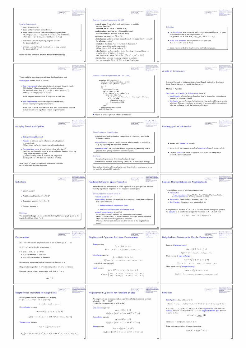
Construction HeuristicsLocal SearchSoftware Tools
Beyond Local OptimaSearch Space PropertiesNeighborhood RepresentationsDistancesEfficient Local SearchMetaheuristics
Iterative Improvement
does not use memory
init: uniform random choice from S
step: uniform random choice from improving neighbors,i.e., step(s, s′) := 1/|I(s)| if s′ ∈ I(s), and 0 otherwise,where I(s) := s′ ∈ S | N (s, s′) and f(s′) < f(s)
terminates when no improving neighbor available(to be revisited later)
different variants through modifications of step function(to be revisited later)
Note: II is also known as iterative descent or hill-climbing.
39
Construction HeuristicsLocal SearchSoftware Tools
Beyond Local OptimaSearch Space PropertiesNeighborhood RepresentationsDistancesEfficient Local SearchMetaheuristics
Example: Iterative Improvement for SAT
search space S: set of all truth assignments to variablesin given formula F(solution set S′: set of all models of F )
neighborhood function N : 1-flip neighborhood(as in Uninformed Random Walk for SAT)
memory: not used, i.e., M := 0initialization: uniform random choice from S, i.e., init(∅, a′) := 1/|S|for all assignments a′
evaluation function: f(a) := number of clauses in Fthat are unsatisfied under assignment a(Note: f(a) = 0 iff a is a model of F .)
step function: uniform random choice from improving neighbors, i.e.,step(a, a′) := 1/#I(a) if s′ ∈ I(a),and 0 otherwise, where I(a) := a′ | N (a, a′) ∧ f(a′) < f(a)termination: when no improving neighbor is availablei.e., terminate(a,>) := 1 if I(a) = ∅, and 0 otherwise.
40
Construction HeuristicsLocal SearchSoftware Tools
Beyond Local OptimaSearch Space PropertiesNeighborhood RepresentationsDistancesEfficient Local SearchMetaheuristics
Definition:
Local minimum: search position without improving neighbors w.r.t. givenevaluation function f and neighborhood N ,i.e., position s ∈ S such that f(s) ≤ f(s′) for all s′ ∈ N(s).
Strict local minimum: search position s ∈ S such thatf(s) < f(s′) for all s′ ∈ N(s).
Local maxima and strict local maxima: defined analogously.
41
Construction HeuristicsLocal SearchSoftware Tools
Beyond Local OptimaSearch Space PropertiesNeighborhood RepresentationsDistancesEfficient Local SearchMetaheuristics
There might be more than one neighbor that have better cost.
Pivoting rule decides which to choose:
Best Improvement (aka gradient descent, steepest descent, greedyhill-climbing): Choose maximally improving neighbor,i.e., randomly select from I∗(s) := s′ ∈ N(s) | f(s′) = f∗,where f∗ := minf(s′) | s′ ∈ N(s).
Note: Requires evaluation of all neighbors in each step.
First Improvement: Evaluate neighbors in fixed order,choose first improving step encountered.
Note: Can be much more efficient than Best Improvement; order ofevaluation can have significant impact on performance.
42
Construction HeuristicsLocal SearchSoftware Tools
Beyond Local OptimaSearch Space PropertiesNeighborhood RepresentationsDistancesEfficient Local SearchMetaheuristics
Example: Iterative Improvement for TSP (2-opt)
procedure TSP-2opt-first(s)input: an initial candidate tour s ∈ S(∈)output: a local optimum s ∈ S(π)
∆ = 0;do
Improvement=FALSE;for i = 1 to n− 2 doif i = 1 then n′ = n− 1 elsen′ = n
for j = i+ 2 to n′ do∆ij = d(ci, cj) + d(ci+1, cj+1)− d(ci, ci+1)− d(cj , cj+1)if ∆ij < 0 then
UpdateTour(s,i,j);Improvement=TRUE;
endend
until Improvement==FALSE;end TSP-2opt-first
ä Are we in a local optimum when it terminates?43
Construction HeuristicsLocal SearchSoftware Tools
Beyond Local OptimaSearch Space PropertiesNeighborhood RepresentationsDistancesEfficient Local SearchMetaheuristicsA note on terminology
Heuristic Methods ≡ Metaheuristics ≡ Local Search Methods ≡ StochasticLocal Search Methods ≡ Hybrid Metaheuristics
Method 6= Algorithm
Stochastic Local Search (SLS) algorithms allude to:
Local Search: informed search based on local or incomplete knowledge asopposed to systematic search
Stochastic: use randomized choices in generating and modifying candidatesolutions. They are introduced whenever it is unknown which deterministicrules are profitable for all the instances of interest.
44
Construction HeuristicsLocal SearchSoftware Tools
Beyond Local OptimaSearch Space PropertiesNeighborhood RepresentationsDistancesEfficient Local SearchMetaheuristicsEscaping from Local Optima
Enlarge the neighborhood
Restart: re-initialize search whenever a local optimumis encountered.(Often rather ineffective due to cost of initialization.)
Non-improving steps: in local optima, allow selection ofcandidate solutions with equal or worse evaluation function value, e.g.,using minimally worsening steps.(Can lead to long walks in plateaus, i.e., regions ofsearch positions with identical evaluation function.)
Note: None of these mechanisms is guaranteed to alwaysescape effectively from local optima.
46
Construction HeuristicsLocal SearchSoftware Tools
Beyond Local OptimaSearch Space PropertiesNeighborhood RepresentationsDistancesEfficient Local SearchMetaheuristics
Diversification vs Intensification
Goal-directed and randomized components of LS strategy need to bebalanced carefully.
Intensification: aims to greedily increase solution quality or probability,e.g., by exploiting the evaluation function.
Diversification: aim to prevent search stagnation by preventing searchprocess from getting trapped in confined regions.
Examples:
Iterative Improvement (II): intensification strategy.
Uninformed Random Walk/Picking (URW/P): diversification strategy.
Balanced combination of intensification and diversification mechanisms formsthe basis for advanced LS methods.
47
Construction HeuristicsLocal SearchSoftware Tools
Beyond Local OptimaSearch Space PropertiesNeighborhood RepresentationsDistancesEfficient Local SearchMetaheuristicsLearning goals of this section
Review basic theoretical concepts
Learn about techniques and goals of experimental search space analysis.
Develop intuition on which features of local search are adequate tocontrast a specific situation.
49
Construction HeuristicsLocal SearchSoftware Tools
Beyond Local OptimaSearch Space PropertiesNeighborhood RepresentationsDistancesEfficient Local SearchMetaheuristicsDefinitions
Search space S
Neighborhood function N : S ⊆ 2S
Evaluation function f(π) : S 7→ R
Problem instance π
Definition:
The search landscape L is the vertex-labeled neighborhood graph given by thetriplet L = (S(π), N(π), f(π)).
50
Construction HeuristicsLocal SearchSoftware Tools
Beyond Local OptimaSearch Space PropertiesNeighborhood RepresentationsDistancesEfficient Local SearchMetaheuristicsFundamental Search Space Properties
The behavior and performance of an LS algorithm on a given problem instancecrucially depends on properties of the respective search space.
Simple properties of search space S:
search space size |S|reachability: solution j is reachable from solution i if neighborhood graphhas a path from i to j.
strongly connected neighborhood graph
weakly optimally connected neighborhood graph
search space diameter diam(GN )(= maximal distance between any two candidate solutions)Note: Diameter of GN = worst-case lower bound for number of searchsteps required for reaching (optimal) solutions.Maximal shortest path between any two vertices in the neighborhoodgraph.
51
Construction HeuristicsLocal SearchSoftware Tools
Beyond Local OptimaSearch Space PropertiesNeighborhood RepresentationsDistancesEfficient Local SearchMetaheuristicsSolution Representations and Neighborhoods
Three different types of solution representations:Permutation
linear permutation: Single Machine Total Weighted Tardiness Problemcircular permutation: Traveling Salesman Problem
Assignment: Graph Coloring Problem, SAT, CSP
Set, Partition: Knapsack, Max Independent Set
A neighborhood function N : S → S × S is also defined through an operator.An operator ∆ is a collection of operator functions δ : S → S such that
s′ ∈ N(s) ⇐⇒ ∃δ ∈ ∆ | δ(s) = s′
53
Construction HeuristicsLocal SearchSoftware Tools
Beyond Local OptimaSearch Space PropertiesNeighborhood RepresentationsDistancesEfficient Local SearchMetaheuristicsPermutations
Π(n) indicates the set all permutations of the numbers 1, 2, . . . , n
(1, 2 . . . , n) is the identity permutation ι.
If π ∈ Π(n) and 1 ≤ i ≤ n then:
πi is the element at position i
posπ(i) is the position of element i
Alternatively, a permutation is a bijective function π(i) = πi
the permutation product π · π′ is the composition (π · π′)i = π′(π(i))
For each π there exists a permutation such that π−1 · π = ι
∆N ⊂ Π
54
Construction HeuristicsLocal SearchSoftware Tools
Beyond Local OptimaSearch Space PropertiesNeighborhood RepresentationsDistancesEfficient Local SearchMetaheuristicsNeighborhood Operators for Linear Permutations
Swap operator∆S = δiS |1 ≤ i ≤ n
δiS(π1 . . . πiπi+1 . . . πn) = (π1 . . . πi+1πi . . . πn)
Interchange operator∆X = δijX |1 ≤ i < j ≤ n
δijX(π) = (π1 . . . πi−1πjπi+1 . . . πj−1πiπj+1 . . . πn)
(≡ set of all transpositions)
Insert operator∆I = δijI |1 ≤ i ≤ n, 1 ≤ j ≤ n, j 6= i
δijI (π) =
(π1 . . . πi−1πi+1 . . . πjπiπj+1 . . . πn) i < j(π1 . . . πjπiπj+1 . . . πi−1πi+1 . . . πn) i > j
55
Construction HeuristicsLocal SearchSoftware Tools
Beyond Local OptimaSearch Space PropertiesNeighborhood RepresentationsDistancesEfficient Local SearchMetaheuristicsNeighborhood Operators for Circular Permutations
Reversal (2-edge-exchange)
∆R = δijR |1 ≤ i < j ≤ nδijR (π) = (π1 . . . πi−1πj . . . πiπj+1 . . . πn)
Block moves (3-edge-exchange)
∆B = δijkB |1 ≤ i < j < k ≤ nδijB (π) = (π1 . . . πi−1πj . . . πkπi . . . πj−1πk+1 . . . πn)
Short block move (Or-edge-exchange)
∆SB = δijSB |1 ≤ i < j ≤ nδijSB(π) = (π1 . . . πi−1πjπj+1πj+2πi . . . πj−1πj+3 . . . πn)
56
Construction HeuristicsLocal SearchSoftware Tools
Beyond Local OptimaSearch Space PropertiesNeighborhood RepresentationsDistancesEfficient Local SearchMetaheuristicsNeighborhood Operators for Assignments
An assignment can be represented as a mappingσ : X1 . . . Xn → v : v ∈ D, |D| = k:
σ = Xi = vi, Xj = vj , . . .One-exchange operator
∆1E = δil1E |1 ≤ i ≤ n, 1 ≤ l ≤ k
δil1E`σ) =
˘σ : σ′(Xi) = vl and σ′(Xj) = σ(Xj) ∀j 6= i
¯Two-exchange operator
∆2E = δij2E |1 ≤ i < j ≤ n
δij2E˘σ : σ′(Xi) = σ(Xj), σ
′(Xj) = σ(Xi) and σ′(Xl) = σ(Xl) ∀l 6= i, j¯
57
Construction HeuristicsLocal SearchSoftware Tools
Beyond Local OptimaSearch Space PropertiesNeighborhood RepresentationsDistancesEfficient Local SearchMetaheuristicsNeighborhood Operators for Partitions or Sets
An assignment can be represented as a partition of objects selected and notselected s : X → C,C(it can also be represented by a bit string)
One-addition operator∆1E = δv1E |v ∈ C
δv1E`s) =
˘s : C′ = C ∪ v and C
′= C \ v
One-deletion operator∆1E = δv1E |v ∈ C
δv1E`s) =
˘s : C′ = C \ v and C
′= C ∪ v
Swap operator∆1E = δv1E |v ∈ C, u ∈ C
δv1E`s) =
˘s : C′ = C ∪ u \ v and C
′= C ∪ v \ u
58
Construction HeuristicsLocal SearchSoftware Tools
Beyond Local OptimaSearch Space PropertiesNeighborhood RepresentationsDistancesEfficient Local SearchMetaheuristicsDistances
Set of paths in GN with s, s′ ∈ S:Φ(s, s′) = (s1, . . . , sh)|s1 = s, sh = s′ ∀i : 1 ≤ i ≤ h− 1, 〈si, si+1〉 ∈ EN
If φ = (s1, . . . , sh) ∈ Φ(s, s′) let |φ| = h be the length of the path; then thedistance between any two solutions s, s′ is the length of shortest path betweens and s′ in GN :
dN (s, s′) = minφ∈Φ(s,s′)
|Φ|
diam(GN ) = maxdN (s, s′) | s, s′ ∈ S
Note: with permutations it is easy to see that:
dN (π, π′) = dN (π−1 · π′, ι)
60

Construction HeuristicsLocal SearchSoftware Tools
Beyond Local OptimaSearch Space PropertiesNeighborhood RepresentationsDistancesEfficient Local SearchMetaheuristics
Distances for Linear Permutation Representations
Swap neighborhood operatorcomputable in O(n2) by the precedence based distance metric:dS(π, π′) = #〈i, j〉|1 ≤ i < j ≤ n, posπ′(πj) < posπ′(πi).diam(GN ) = n(n− 1)/2
Interchange neighborhood operatorComputable in O(n) +O(n) sincedX(π, π′) = dX(π−1 · π′, ι) = n− c(π−1 · π′)where c(π) is the number of disjoint cycles that decompose a permutation.diam(GNX ) = n− 1
Insert neighborhood operatorComputable in O(n) +O(n log(n)) sincedI(π, π
′) = dI(π−1 · π′, ι) = n− |lis(π−1 · π′)| where lis(π) denotes the
length of the longest increasing subsequence.diam(GNI ) = n− 1
61
Construction HeuristicsLocal SearchSoftware Tools
Beyond Local OptimaSearch Space PropertiesNeighborhood RepresentationsDistancesEfficient Local SearchMetaheuristics
Distances for Circular Permutation Representations
Reversal neighborhood operatorsorting by reversal is known to be NP-hardsurrogate in TSP: bond distance
Block moves neighborhood operatorunknown whether it is NP-hard but there does not exist a provedpolynomial-time algorithm
62
Construction HeuristicsLocal SearchSoftware Tools
Beyond Local OptimaSearch Space PropertiesNeighborhood RepresentationsDistancesEfficient Local SearchMetaheuristics
Distances for Assignment Representations
Hamming Distance
An assignment can be seen as a partition of n in k mutually exclusivenon-empty subsets
One-exchange neighborhood operatorThe partition-distance d1E(P,P ′) between two partitions P and P ′ is theminimum number of elements that must be moved between subsets in Pso that the resulting partition equals P ′.The partition-distance can be computed in polynomial time by solving anassignment problem. Given the assignment matrix M where in each cell(i, j) it is |Si ∩ S′j | with Si ∈ P and S′j ∈ P ′ and defined A(P,P ′) theassignment of maximal sum then it is d1E(P,P ′) = n−A(P,P ′)
63
Construction HeuristicsLocal SearchSoftware Tools
Beyond Local OptimaSearch Space PropertiesNeighborhood RepresentationsDistancesEfficient Local SearchMetaheuristics
Example: Search space size and diameter for the TSP
Search space size = (n− 1)!/2
Insert neighborhoodsize = (n− 3)ndiameter = n− 2
2-exchange neighborhoodsize =
`n2
´= n · (n− 1)/2
diameter in [n/2, n− 2]
3-exchange neighborhoodsize =
`n3
´= n · (n− 1) · (n− 2)/6
diameter in [n/3, n− 1]
64
Construction HeuristicsLocal SearchSoftware Tools
Beyond Local OptimaSearch Space PropertiesNeighborhood RepresentationsDistancesEfficient Local SearchMetaheuristics
Example: Search space size and diameter for SAT
SAT instance with n variables, 1-flip neighborhood:GN = n-dimensional hypercube; diameter of GN = n.
65
Construction HeuristicsLocal SearchSoftware Tools
Beyond Local OptimaSearch Space PropertiesNeighborhood RepresentationsDistancesEfficient Local SearchMetaheuristics
Let N1 and N2 be two different neighborhood functions for the same instance(S, f, π) of a combinatorial optimization problem.
If for all solutions s ∈ S we have N1(s) ⊆ N2(s′) then we say that N2
dominates N1
Example:
In TSP, 1-insert is domnated by 3-exchange.(1-insert corresponds to 3-exchange and there are 3-exchnages that are not1-insert)
66
Construction HeuristicsLocal SearchSoftware Tools
Beyond Local OptimaSearch Space PropertiesNeighborhood RepresentationsDistancesEfficient Local SearchMetaheuristicsEfficiency vs Effectiveness
The performance of local search is determined by:
1. quality of local optima (effectiveness)
2. time to reach local optima (efficiency):
A. time to move from one solution to the next
B. number of solutions to reach local optima
68
Construction HeuristicsLocal SearchSoftware Tools
Beyond Local OptimaSearch Space PropertiesNeighborhood RepresentationsDistancesEfficient Local SearchMetaheuristics
Note:
Local minima depend on g and neighborhood function N .Larger neighborhoods N induce
neighborhood graphs with smaller diameter;fewer local minima.
Ideal case: exact neighborhood, i.e., neighborhood functionfor which any local optimum is also guaranteed to bea global optimum.
Typically, exact neighborhoods are too large to be searched effectively(exponential in size of problem instance).
But: exceptions exist, e.g., polynomially searchable neighborhood inSimplex Algorithm for linear programming.
69
Construction HeuristicsLocal SearchSoftware Tools
Beyond Local OptimaSearch Space PropertiesNeighborhood RepresentationsDistancesEfficient Local SearchMetaheuristics
Trade-off (to be assessed experimentally):
Using larger neighborhoodscan improve performance of II (and other LS methods).
But: time required for determining improving search stepsincreases with neighborhood size.
Speedups Techniques for Efficient Neighborhood Search
1) Incremental updates
2) Neighborhood pruning
70
Construction HeuristicsLocal SearchSoftware Tools
Beyond Local OptimaSearch Space PropertiesNeighborhood RepresentationsDistancesEfficient Local SearchMetaheuristicsSpeedups in Neighborhood Examination
1) Incremental updates (aka delta evaluations)
Key idea: calculate effects of differences betweencurrent search position s and neighbors s′ onevaluation function value.
Evaluation function values often consist ofindependent contributions of solution components;hence, f(s) can be efficiently calculated from f(s′) by differences betweens and s′ in terms of solution components.
Typically crucial for the efficient implementation ofII algorithms (and other LS techniques).
71
Construction HeuristicsLocal SearchSoftware Tools
Beyond Local OptimaSearch Space PropertiesNeighborhood RepresentationsDistancesEfficient Local SearchMetaheuristics
Example: Incremental updates for TSP
solution components = edges of given graph G
standard 2-exchange neighborhood, i.e., neighboringround trips p, p′ differ in two edges
w(p′) := w(p) − edges in p but not in p′
+ edges in p′ but not in p
Note: Constant time (4 arithmetic operations), compared tolinear time (n arithmetic operations for graph with n vertices)for computing w(p′) from scratch.
72
Construction HeuristicsLocal SearchSoftware Tools
Beyond Local OptimaSearch Space PropertiesNeighborhood RepresentationsDistancesEfficient Local SearchMetaheuristics
2) Neighborhood Pruning
Idea: Reduce size of neighborhoods by excluding neighbors that are likely(or guaranteed) not to yield improvements in f .
Note: Crucial for large neighborhoods, but can be also very useful forsmall neighborhoods (e.g., linear in instance size).
Example: Heuristic candidate lists for the TSP
Intuition: High-quality solutions likely include short edges.
Candidate list of vertex v: list of v’s nearest neighbors (limited number),sorted according to increasing edge weights.
Search steps (e.g., 2-exchange moves) always involve edges to elements ofcandidate lists.
Significant impact on performance of LS algorithmsfor the TSP.
73
Construction HeuristicsLocal SearchSoftware Tools
Beyond Local OptimaSearch Space PropertiesNeighborhood RepresentationsDistancesEfficient Local SearchMetaheuristicsOverview
Delta evaluations and neighborhood examinations in:
PermutationsTSPSMTWTP
AssignmentsSAT
SetsMax Independent Set
74
Construction HeuristicsLocal SearchSoftware Tools
Beyond Local OptimaSearch Space PropertiesNeighborhood RepresentationsDistancesEfficient Local SearchMetaheuristicsLocal Search for TSP
k-exchange heuristics2-opt2.5-optOr-opt3-opt
complex neighborhoodsLin-KernighanHelsgaun’s Lin-KernighanDynasearchejection chains approach
Implementations exploit speed-up techniques
1 neighborhood pruning: fixed radius nearest neighborhood search
2 neighborhood lists: restrict exchanges to most interesting candidates
3 don’t look bits: focus perturbative search to “interesting” part
4 sophisticated data structures
75
Construction HeuristicsLocal SearchSoftware Tools
Beyond Local OptimaSearch Space PropertiesNeighborhood RepresentationsDistancesEfficient Local SearchMetaheuristics
TSP data structures
Tour representation:
determine pos of v in π
determine succ and prec
check whether uk is visited between ui and ujexecute a k-exchange (reversal)
Possible choices:
|V | < 1.000 array for π and π−1
|V | < 1.000.000 two level tree
|V | > 1.000.000 splay tree
Moreover static data structure:
priority lists
k-d trees
76
Construction HeuristicsLocal SearchSoftware Tools
Beyond Local OptimaSearch Space PropertiesNeighborhood RepresentationsDistancesEfficient Local SearchMetaheuristics
SMTWTP
Interchange: size`n2
´and O(|i− j|) evaluation each
first-improvement: πj , πkpπj ≤ pπk for improvements, wjTj +wkTk must decrease because jobs
in πj , . . . , πk can only increase their tardiness.pπj ≥ pπk possible use of auxiliary data structure to speed up the com-
putationfirst-improvement: πj , πkpπj ≤ pπk for improvements, wjTj + wkTk must decrease at least as
the best interchange found so far because jobs in πj , . . . , πkcan only increase their tardiness.
pπj ≥ pπk possible use of auxiliary data structure to speed up the com-putation
Swap: size n− 1 and O(1) evaluation each
Insert: size (n− 1)2 and O(|i− j|) evaluation eachBut possible to speed up with systematic examination by means of swaps:an interchange is equivalent to |i− j| swaps hence overall examinationtakes O(n2)
77
Construction HeuristicsLocal SearchSoftware Tools
Beyond Local OptimaSearch Space PropertiesNeighborhood RepresentationsDistancesEfficient Local SearchMetaheuristicsLS for GCP
search space S: set of all k-colorings of G
solution set S′: set of all proper k-coloring of F
neighborhood function N : 1-exchange neighborhood(as in Uninformed Random Walk)
memory: not used, i.e., M := 0initialization: uniform random choice from S, i.e., init∅, ϕ′ := 1/|S|for all colorings ϕ′
step function:evaluation function: g(ϕ) := number of edges in Gwhose ending vertices are assigned the same color under assignment ϕ(Note: g(ϕ) = 0 iff ϕ is a proper coloring of G.)move mechanism: uniform random choice from improving neighbors, i.e.,stepϕ,ϕ′ := 1/|I(ϕ)| if s′ ∈ I(ϕ),and 0 otherwise, where I(ϕ) := ϕ′ | N (ϕ,ϕ′) ∧ g(ϕ′) < g(ϕ)
termination: when no improving neighbor is availablei.e., terminateϕ,> := 1 if I(ϕ) = ∅, and 0 otherwise.
78
Construction HeuristicsLocal SearchSoftware Tools
Beyond Local OptimaSearch Space PropertiesNeighborhood RepresentationsDistancesEfficient Local SearchMetaheuristicsTabu Search
Key idea: Use aspects of search history (memory) to escape from local minima.
Associate tabu attributes with candidate solutions orsolution components.
Forbid steps to search positions recently visited byunderlying iterative best improvement procedure based ontabu attributes.
Tabu Search (TS):determine initial candidate solution sWhile termination criterion is not satisfied:|| determine set N ′ of non-tabu neighbors of s|| choose a best improving candidate solution s′ in N ′|||| update tabu attributes based on s′b s := s′
80

Construction HeuristicsLocal SearchSoftware Tools
Beyond Local OptimaSearch Space PropertiesNeighborhood RepresentationsDistancesEfficient Local SearchMetaheuristics
Note:
Non-tabu search positions in N(s) are calledadmissible neighbors of s.
After a search step, the current search positionor the solution components just added/removed from itare declared tabu for a fixed number of subsequentsearch steps (tabu tenure).
Often, an additional aspiration criterion is used: this specifiesconditions under which tabu status may be overridden (e.g., ifconsidered step leads to improvement in incumbent solution).
Crucial for efficient implementation:keep time complexity of search steps minimalby using special data structures, incremental updatingand caching mechanism for evaluation function values;efficient determination of tabu status:store for each variable x the number of the search stepwhen its value was last changed itx; x is tabu ifit− itx < tt, where it = current search step number.
81
Construction HeuristicsLocal SearchSoftware Tools
Beyond Local OptimaSearch Space PropertiesNeighborhood RepresentationsDistancesEfficient Local SearchMetaheuristics
Note: Performance of Tabu Search depends crucially onsetting of tabu tenure tt:
tt too low ⇒ search stagnates due to inability to escapefrom local minima;
tt too high ⇒ search becomes ineffective due to overly restricted searchpath (admissible neighborhoods too small)
82
Construction HeuristicsLocal SearchSoftware Tools
Beyond Local OptimaSearch Space PropertiesNeighborhood RepresentationsDistancesEfficient Local SearchMetaheuristicsIterated Local Search
Key Idea: Use two types of LS steps:subsidiary local search steps for reachinglocal optima as efficiently as possible (intensification)
perturbation steps for effectivelyescaping from local optima (diversification).
Also: Use acceptance criterion to control diversification vs intensificationbehavior.
Iterated Local Search (ILS):determine initial candidate solution sperform subsidiary local search on sWhile termination criterion is not satisfied:|| r := s|| perform perturbation on s|| perform subsidiary local search on s|||| based on acceptance criterion,b keep s or revert to s := r
83
Construction HeuristicsLocal SearchSoftware Tools
The Code DeliveredPractical Exercise
Outline1. Construction Heuristics
General PrinciplesMetaheuristics
A∗ searchRolloutBeam SearchIterated GreedyGRASP
2. Local SearchBeyond Local OptimaSearch Space PropertiesNeighborhood RepresentationsDistancesEfficient Local Search
Efficiency vs EffectivenessApplication Examples
MetaheuristicsTabu SearchIterated Local Search
3. Software ToolsThe Code DeliveredPractical Exercise
84
Construction HeuristicsLocal SearchSoftware Tools
The Code DeliveredPractical Exercise
Software Tools
Modeling languagesinterpreted languages with a precise syntax and semantics
Software librariescollections of subprograms used to develop software
Software frameworksset of abstract classes and their interactions
frozen spots (remain unchanged in any instantiation of the framework)
hot spots (parts where programmers add their own code)
85
Construction HeuristicsLocal SearchSoftware Tools
The Code DeliveredPractical Exercise
No well established software tool for Local Search:
the apparent simplicity of Local Search induces to build applications fromscratch.
crucial roles played by delta/incremental updates which is problemdependent
the development of Local Search is in part a craft,beside engineering and science.
lack of a unified view of Local Search.
86
Construction HeuristicsLocal SearchSoftware Tools
The Code DeliveredPractical Exercise
Software tools for Local Search and Metaheuristics
Tool Reference Language TypeILOG ? C++, Java, .NET LSGAlib ? C++ GAGAUL ? C GALocalizer++ ? C++ ModelingHotFrame ? C++ LSEasyLocal++ ? C++, Java LSHSF ? Java LS, GAParadisEO ? C++ EA, LSOpenTS ? Java TSMDF ? C++ LSTMF ? C++ LSSALSA ? — LanguageComet ? — Language
table prepared by L. Di Gaspero
87
Construction HeuristicsLocal SearchSoftware Tools
The Code DeliveredPractical Exercise
Separation of Concepts in Local Search Algorithms
implemented in EasyLocal++
88
Construction HeuristicsLocal SearchSoftware Tools
The Code DeliveredPractical Exercise
Input (util.h, util.c)
typedef struct long int number_jobs; /∗ number of jobs in instance ∗/long int release_date[MAX_JOBS]; /∗there is no release date for these instances∗/long int proc_time[MAX_JOBS];long int weight[MAX_JOBS];long int due_date[MAX_JOBS];
instance_type;
instance_type instance;
void read_problem_size (char name[100])void read_instances (char input_file_name[100])
90
Construction HeuristicsLocal SearchSoftware Tools
The Code DeliveredPractical Exercise
State/Solution (util.h)
typedef struct long int job_at_pos[MAX_JOBS]; /∗ Gives the job at a certain pos ∗/long int pos_of_job[MAX_JOBS]; /∗ Gives the position of a specific job ∗/long int completion_time_job[MAX_JOBS]; /∗ Gives C_j of job j ∗/long int start_time_job[MAX_JOBS]; /∗ Gives start time of job j ∗/long int tardiness_job[MAX_JOBS]; /∗ Gives T_j of job j ∗/long int value; /∗ Objective function value ∗/
sol_representation;
sol_representation sequence;
Output (util.c)
void print_sequence (long int k)void print_completion_times ()
State Manager (util.c)
void construct_sequence_random ()void construct_sequence_canonical ()long int evaluate ()
91
Construction HeuristicsLocal SearchSoftware Tools
The Code DeliveredPractical Exercise
Random Generator (random.h, random.c)
void set_seed (double arg)double MRG32k3a (void)double ranU01 (void)int ranUint (int i, int j)void shuffle (int *X, int size)
Timer (timer.c)
double getCurrentTime ()
92
Your Task on 1|| ∑j wjTj1|| ∑j wjTj1|| ∑j wjTj
Implement two basic local search procedures that return a local optimum:
void ls_swap_first( ) ;void ls_interchange_first( ) ;
Implement the other neighborhood for permutation representationmentioned at the lecture from one of the two previous neighborhoods.Provide computational analysis of the LS implemented. Consider:
size of the neighborhooddiameter of neighborhoodcomplete neighborhood examinationlocal optima attainment
Devise speed ups to reduce the computational complexity of the LSimplemented
Improve your heuristic in order to find solutions of better quality. (Hint:use a construction heuristic and/or a metaheuristic)

DMP204SCHEDULING,
TIMETABLING AND ROUTING
Lecture 9
Heuristics
Marco Chiarandini
AntsOutline
1. AntsAdaptive Iterated Construction Search
2
Ants Adaptive Iterated Construction SearchOutline
1. AntsAdaptive Iterated Construction Search
3
Ants Adaptive Iterated Construction SearchAdaptive Iterated Construction Search
Key Idea: Alternate construction and perturbative local search phases asin GRASP, exploiting experience gained during the search process.
Realisation:
Associate weights with possible decisions made during constructivesearch.
Initialize all weights to some small value τ0 at beginning of searchprocess.
After every cycle (= constructive + perturbative local search phase),update weights based on solution quality and solution componentsof current candidate solution.
5
Ants Adaptive Iterated Construction Search
Adaptive Iterated Construction Search (AICS):initialise weightsWhile termination criterion is not satisfied:|| generate candidate solution s using|| subsidiary randomized constructive search|||| perform subsidiary local search on s||b adapt weights based on s
6
Ants Adaptive Iterated Construction Search
Subsidiary constructive search:
The solution component to be added in each step of constructivesearch is based on weights andheuristic function h.
h can be standard heuristic function as, e.g., used bygreedy construction heuristics, GRASP or tree search.
It is often useful to design solution component selection inconstructive search such that any solution component may bechosen (at least with some small probability) irrespective ofits weight and heuristic value.
7
Ants Adaptive Iterated Construction Search
Subsidiary perturbative local search:
As in GRASP, perturbative local search phase is typically importantfor achieving good performance.
Can be based on Iterative Improvement or more advanced LSmethod (the latter often results in better performance).
Tradeoff between computation time used in construction phase vslocal search phase (typically optimized empirically, depends onproblem domain).
8
Ants Adaptive Iterated Construction Search
Weight updating mechanism:
Typical mechanism: increase weights of all solution componentscontained in candidate solution obtained from local search.
Can also use aspects of search history; e.g., current incumbentcandidate solution can be used as basis forweight update for additional intensification.
9
Ants Adaptive Iterated Construction Search
Example: A simple AICS algorithm for the TSP (1)
(Based on Ant System for the TSP [Dorigo et al., 1991])
Search space and solution set as usual (all Hamiltonian cycles ingiven graph G).
Associate weight τij with each edge (i, j) in G.
Use heuristic values ηij := 1/w((i, j)).
Initialize all weights to a small value τ0 (parameter).
Constructive search starts with randomly chosen vertexand iteratively extends partial round trip φ by selecting vertexnot contained in φ with probability
[τij ]α · [ηij ]β∑l∈N ′(i)[τil]α · [ηij ]β
10
Ants Adaptive Iterated Construction Search
Example: A simple AICS algorithm for the TSP (2)
Subsidiary local search = iterative improvement based on standard2-exchange neighborhood (until local minimumis reached).
Weight update according to
τij := (1− ρ) · τij + ∆(i, j, s′)
where ∆(i, j, s′) := 1/f(s′), if edge (i, j) is contained inthe cycle represented by s′, and 0 otherwise.
Criterion for weight increase is based on intuition that edgescontained in short round trips should be preferably used insubsequent constructions.
11

DMP204SCHEDULING,
TIMETABLING AND ROUTING
Lecture 10
Single Machine Models, DynamicProgramming
Marco Chiarandini
Dispatching RulesSingle Machine ModelsOutline
1. Dispatching Rules
2. Single Machine Models
2
Dispatching RulesSingle Machine ModelsOutline
1. Dispatching Rules
2. Single Machine Models
3
Dispatching RulesSingle Machine ModelsDispatching rules
Distinguish static and dynamic rules.
Service in random order (SIRO)
Earliest release date first (ERD=FIFO)tends to min variations in waiting time
Earliest due date (EDD)
Minimal slack first (MS)j∗ = arg minjmax(dj − pj − t, 0).tends to min due date objectives (T,L)
4
Dispatching RulesSingle Machine Models
(Weighted) shortest processing time first (WSPT)j∗ = arg maxjwj/pj.tends to min
PwjCj and max work in progress and
Loongest processing time first (LPT)balance work load over parallel machines
Shortest setup time first (SST)tends to min Cmax and max throughput
Least flexible job first (LFJ)eligibility constraints
5
Dispatching RulesSingle Machine Models
Critical path (CP)first job in the CP
tends to min Cmax
Largest number of successors (LNS)
Shortest queue at the next operation (SQNO)tends to min idleness of machines
6
Dispatching RulesSingle Machine ModelsDispatching Rules in Scheduling
RULE DATA OBJECTIVESRules Dependent ERD rj Variance in Throughput Timeson Release Dates EDD dj Maximum Latenessand Due Dates MS dj Maximum Lateness
LPT pj Load Balancing over Parallel MachinesRules Dependent SPT pj Sum of Completion Times, WIPon Processing WSPT pj , wj Weighted Sum of Completion Times, WIPTimes CP pj , prec Makespan
LNS pj , prec MakespanSIRO - Ease of Implementation
Miscellaneous SST sjk Makespan and ThroughputLFJ Mj Makespan and ThroughputSQNO - Machine Idleness
7
Dispatching RulesSingle Machine Models
When dispatching rules are optimal?
8
Dispatching RulesSingle Machine ModelsComposite dispatching rules
Why composite rules?
Example: 1 | | ∑wjTj :
WSPT, optimal if due dates are zero
EDD, optimal if due dates are loose
MS, tends to minimize T
ä The efficacy of the rules depends on instance factors
9
Dispatching RulesSingle Machine Models
Instance characterizationJob attributes: weight, processing time, due date, release date
Machine attributes: speed, num. of jobs waiting, num. of jobseligible
Possible instance factors:
1 | |PwjTj
θ1 = 1− d
Cmax(due date tightness)
θ2 =dmax − dmin
Cmax(due date range)
1 | sjk|PwjTj
(θ1, θ2 with estimated Cmax =
nXj=1
pj + ns)
θ3 =s
p(set up time severity)
10
Dispatching RulesSingle Machine Models
1 | |∑wjTj , dynamic apparent tardiness cost (ATC)
Ij(t) =wjpj
exp(−max(dj − pj − t, 0)
Kp
)1 | sjk|
∑wjTj , dynamic apparent tardiness cost with setups (ATCS)
Ij(t, l) =wjpj
exp(−max(dj − pj − t, 0)
K1p
)exp
(−sjkK2s
)after job l has finished.
11
Dispatching RulesSingle Machine ModelsSummary
Scheduling classification
Solution methods
Practice with general solution methodsMathematical Programming
Constraint Programming
Heuristic methods
12
Dispatching RulesSingle Machine ModelsOutlook on Scheduling
Objectives:Look closer into scheduling models and learn:
special algorithms
application of general methods
Cases:
Single Machine
Parallel Machine
Permutation Flow Shop
Job Shop
Resource Constrained Project Scheduling
13
Dispatching RulesSingle Machine ModelsOutline
1. Dispatching Rules
2. Single Machine Models
14
Dispatching RulesSingle Machine ModelsOutlook
1 | | ∑wjCj : weighted shortest processing time first is optimal
1 | | ∑j Uj : Moore’s algorithm
1 | prec| Lmax : Lawler’s algorithm, backward dynamic programming inO(n2) [Lawler, 1973]
1 | | ∑hj(Cj) : dynamic programming in O(2n)
1 | | ∑wjTj : local search and dynasearch
1 | rj , (prec) | Lmax : branch and bound
1 | sjk | Cmax : in the special case, Gilmore and Gomory algorithmoptimal in O(n2)
1 | | ∑wjTj : column generation approaches
Multicriteria 15
Dispatching RulesSingle Machine ModelsSummary
Single Machine Models:
Cmax is sequence independent
if rj = 0 and hj is monotone non decreasing in Cj then optimalschedule is nondelay and has no preemption.
16
Dispatching RulesSingle Machine Models1 | | ∑wjCj1 | | ∑wjCj1 | | ∑wjCj
[Total weighted completion time]
Theorem: The weighted shortest processing time first (WSPT) rule isoptimal.
Extensions to 1 | prec | ∑wjCj
in the general case strongly NP-hard
chain precedences:process first chain with highest ρ-factor up to, and included, jobwith highest ρ-factor.
polytime algorithm also for tree and sp-graph precedences
17
Dispatching RulesSingle Machine Models
Extensions to 1 | rj , prmp |∑wjCj
in the general case strongly NP-hard
preemptive version of the WSPT if equal weights
however, 1 | rj |∑wjCj is strongly NP-hard
18

Dispatching RulesSingle Machine Models1 | | ∑j Uj1 | | ∑j Uj1 | | ∑j Uj
[Number of tardy jobs]
[Moore, 1968] algorithm in O(n log n)
Add jobs in increasing order of due dates
If inclusion of job j∗ results in this job being completed latediscard the scheduled job k∗ with the longest processing time
1 | | ∑j wjUj is a knapsack problem hence NP-hard
19
Dispatching RulesSingle Machine ModelsDynamic programming
Procedure based on divide and conquer
Principle of optimality the completion of an optimal sequence of decisionsmust be optimal
Break down the problem into stages at which the decisions takeplaceFind a recurrence relation that takes us backward (forward) fromone stage to the previous (next)
(In scheduling, backward procedure feasible only if the makespan isschedule, eg, single machine problems without setups, multiple machinesproblems with identical processing times.)
20
Dispatching RulesSingle Machine Models1 | prec| hmax1 | prec| hmax1 | prec| hmax
hmax = maxh1(C1), h2(C2), . . . , hn(Cn), hj regular
special case: 1 | prec| hmax [maximum lateness]
solved by backward dynamic programming in O(n2) [Lawler, 1978]
J set of jobs already scheduled;Jc set of jobs still to schedule;J ′ ⊆ Jc set of schedulable jobs
Step 1: Set J = ∅, Jc = 1, . . . , n and J ′ the set of all jobs withno successor
Step 2: Select j∗ such that j∗ = arg minj∈J′hj(∑
k∈Jc pk);
add j∗ to J ; remove j∗ from Jc; update J ′.Step 3: If Jc is empty then stop, otherwise go to Step 2.
For 1 | | Lmax Earliest Due Date first
1|rj |Lmax is instead strongly NP-hard21
Dispatching RulesSingle Machine Models1 | | ∑hj(Cj)1 | | ∑hj(Cj)1 | | ∑hj(Cj)
generalization of∑wjTj hence strongly NP-hard
(forward) dynamic programming algorithm O(2n)
J set of job already scheduled;
V (J) =∑j∈J hj(Cj)
Step 1: Set J = ∅, V (j) = hj(pj), j = 1, . . . , n
Step 2: V (J) = minj∈J(V (J − j) + hj
(∑k∈J pk
))Step 3: If J = 1, 2, . . . , n then V (1, 2, . . . , n) is optimum,
otherwise go to Step 2.
22
Dispatching RulesSingle Machine Models1 | | ∑hj(Cj)1 | | ∑hj(Cj)1 | | ∑hj(Cj)
A lot of work done on 1 | | ∑wjTj[single-machine total weighted tardiness]
1 | | ∑Tj is hard in ordinary sense, hence admits a pseudopolynomial algorithm (dynamic programming in O(n4
∑pj))
1 | | ∑wjTj strongly NP-hard (reduction from 3-partition)
exact solution via branch and bound feasible up to 40 jobs[Potts and Wassenhove, Oper. Res., 1985]
exact solution via time-indexed integer programming formulationused to lower bound in branch and bound solves instances of 100jobs in 4-9 hours [Pan and Shi, Math. Progm., 2007]
dynasearch: results reported for 100 jobs within a 0.005% gap fromoptimum in less than 3 seconds [Grosso et al., Oper. Res. Lett.,2004]
23
Dispatching RulesSingle Machine Models1 | | ∑hj(Cj)1 | | ∑hj(Cj)1 | | ∑hj(Cj)
Local search
Interchange: size(n2
)and O(|i− j|) evaluation each
first-improvement: πj , πkpπj ≤ pπk for improvements, wjTj +wkTk must decrease because
jobs in πj , . . . , πk can only increase their tardiness.pπj ≥ pπk possible use of auxiliary data structure to speed up the
computationbest-improvement: πj , πkpπj ≤ pπk for improvements, wjTj + wkTk must decrease at least
as the best interchange found so far because jobs inπj , . . . , πk can only increase their tardiness.
pπj ≥ pπk possible use of auxiliary data structure to speed up thecomputation
Swap: size n− 1 and O(1) evaluation eachInsert: size (n− 1)2 and O(|i− j|) evaluation eachBut possible to speed up with systematic examination by means ofswaps: an interchange is equivalent to |i− j| swaps hence overallexamination takes O(n2)
25
Dispatching RulesSingle Machine Models
Dynasearch
two interchanges δjk and δlm are independentif maxj, k < minl,m or minl, k > maxl,m;
the dynasearch neighborhood is obtained by a series of independentinterchanges;
it has size 2n−1 − 1;
but a best move can be found in O(n3) searched by dynamicprogramming;
it yields in average better results than the interchange neighborhoodalone.
26
Dispatching RulesSingle Machine Models
state (k, π)
πk is the partial sequence at state (k, π) that has min∑wT
πk is obtained from state (i, π)appending job π(k) after π(i) i = k − 1appending job π(k) and interchanging π(i+ 1) and π(k) 0 ≤ i < k − 1
F (π0) = 0; F (π1) = wπ(1)
(pπ(1) − dπ(1)
)+;
F (πk) = min
F (πk−1) + wπ(k)
(Cπ(k) − dπ(k)
)+,
min1≤i<k−1
F (πi) + wπ(k)
(Cπ(i) + pπ(k) − dπ(k)
)+ +
+∑k−1j=i+2 wπ(j)
(Cπ(j) + pπ(k) − pπ(i+1) − dπ(j)
)+ ++wπ(i+1)
(Cπ(k) − dπ(i+1)
)+27
Dispatching RulesSingle Machine Models
The best choice is computed by recursion in O(n3) and the optimalseries of interchanges for F (πn) is found by backtrack.
Local search with dynasearch neighborhood starts from an initialsequence, generated by ATC, and at each iteration applies the bestdynasearch move, until no improvement is possible (that is,F (πtn) = F (π(t−1)
n ), for iteration t).
Speedups:pruning with considerations on pπ(k) and pπ(i+1)
maintainig a string of late, no late jobs
ht largest index s.t. π(t−1)(k) = π(t−2)(k) for k = 1, . . . , ht thenF (π
(t−1)k ) = F (π
(t−2)k ) for k = 1, . . . , ht and at iter t no need to
consider i < ht.
28
Dispatching RulesSingle Machine Models
Dynasearch, refinements:
[Grosso et al. 2004] add insertion moves to interchanges.
[Ergun and Orlin 2006] show that dynasearch neighborhood can besearched in O(n2).
29
Dispatching RulesSingle Machine Models1 | rj | Lmax1 | rj | Lmax1 | rj | Lmax
[Maximum lateness with release dates]
Strongly NP-hard (reduction from 3-partition)
might have optimal schedule which is not non-delay
Branch and bound algorithm (valid also for 1 | rj , prec | Lmax)Branching:schedule from the beginning (level k, n!/(k − 1)! nodes)elimination criterion: do not consider job jk if:
rj > minl∈Jmax (t, rl) + pl J jobs to schedule, t current time
Lower bounding: relaxation to preemptive case for which EDD isoptimal
31
Dispatching RulesSingle Machine Models
Branch and BoundS root of the branching tree
1 LIST := S;2 U:=value of some heuristic solution;3 current_best := heuristic solution;4 while LIST 6= ∅5 Choose a branching node k from LIST;6 Remove k from LIST;7 Generate children child(i), i = 1, . . . , nk, and calculate corresponding
lower bounds LBi;8 for i:=1 to nk9 if LBi < U then10 if child(i) consists of a single solution then11 U :=LBi;12 current_best:=solution corresponding to child(i)13 else add child(i) to LIST
32

DMP204SCHEDULING,
TIMETABLING AND ROUTING
Lecture 11
Single Machine Models, Branch and Bound
Marco Chiarandini
Single Machine ModelsOutline
1. Single Machine ModelsBranch and Bound1 | sjk |Cmax
2
Single Machine Models Branch and Bound1 | sjk |CmaxOutline
1. Single Machine ModelsBranch and Bound1 | sjk |Cmax
3
Single Machine Models Branch and Bound1 | sjk |Cmax1 | rj | Lmax1 | rj | Lmax1 | rj | Lmax
[Maximum lateness with release dates]
Strongly NP-hard (reduction from 3-partition)
might have optimal schedule which is not non-delay
Branch and bound algorithm (valid also for 1 | rj , prec | Lmax)Branching:schedule from the beginning (level k, n!/(k − 1)! nodes)elimination criterion: do not consider job jk if:
rj > minl∈Jmax (t, rl) + pl J jobs to schedule, t current time
Lower bounding: relaxation to preemptive case for which EDD isoptimal
5
Single Machine Models Branch and Bound1 | sjk |Cmax
Branch and BoundS root of the branching tree
1 LIST := S;2 U:=value of some heuristic solution;3 current_best := heuristic solution;4 while LIST 6= ∅5 Choose a branching node k from LIST;6 Remove k from LIST;7 Generate children child(i), i = 1, . . . , nk, and calculate corresponding lower
bounds LBi;8 for i:=1 to nk
9 if LBi < U then10 if child(i) consists of a single solution then11 U :=LBi;12 current_best:=solution corresponding to child(i)13 else add child(i) to LIST
6
Single Machine Models Branch and Bound1 | sjk |CmaxBranch and Bound
[Jens Clausen (1999). Branch and Bound Algorithms- Principles and Examples.]
Eager Strategy:1. select a node2. branch3. for each subproblem compute bounds and compare with
incumbent solution4. discard or store nodes together with their bounds
(Bounds are calculated as soon as nodes are available)
Lazy Strategy:1. select a node2. compute bound3. branch4. store the new nodes together with the bound of the processed
node
(often used when selection criterion for next node is max depth)7
Single Machine Models Branch and Bound1 | sjk |Cmax
Components
- Initial feasible solution (heuristic) – might be crucial!1. Bounding function2. Strategy for selecting3. Branching- Fathmoing (dominance test)
8
Single Machine Models Branch and Bound1 | sjk |Cmax
Bounding
mins∈P
g(s) ≤
mins∈P f(s)mins∈S g(s)
≤ min
s∈Sf(s)
P : candidate solutions; S ⊆ P feasible solutions
relaxation: mins∈P f(s)solve (to optimality) in P but with g
Lagrangian relaxation combines the two
should be polytime and strong (trade off)
9
Single Machine Models Branch and Bound1 | sjk |Cmax
Strategy for selecting next subproblem
best first(combined with eager strategy but also with lazy)
breadth first(memory problems)
depth firstworks on recursive updates (hence good for memory)but might compute a large part of the tree which is far from optimal(enhanced by alternating search in lowest and largest boundscombined with branching on the node with the largest difference inbound between the children)(it seems to perform best)
10
Single Machine Models Branch and Bound1 | sjk |Cmax
Branching
dichotomic
polytomic
Overall guidelines
finding good initial solutions is important
if initial solution is close to optimum then the selection strategymakes little difference
Parallel B&B: distributed control or a combination are better thancentralized control
parallelization might be used also to compute bounds if few nodesalive
parallelization with static work load distribution is appealing withlarge search trees
11
Single Machine Models Branch and Bound1 | sjk |Cmax
Branch and bound vs backtracking
= a state space tree is used to solve a problem.
6= branch and bound does not limit us to any particular way oftraversing the tree (backtracking is depth-first)
6= branch and bound is used only for optimization problems.
Branch and bound vs A∗
= In A∗ the admissible heuristic mimics bounding
6= In A∗ there is no branching. It is a search algorithm.
6= A∗ is best first
12
Single Machine Models Branch and Bound1 | sjk |Cmax1 | | ∑wjTj1 | | ∑wjTj1 | | ∑wjTj
Branching:work backward in time
elimination criterion:if pj ≤ pk and dj ≤ dk and wj ≥ wk then there is an optimalschedule with j before k
Lower Bounding:relaxation to preemptive casetransportation problem
minn∑j=1
Cmax∑t=1
cjtxjt
s.t.Cmax∑t=1
xjt = pj , ∀j = 1, . . . , n
n∑j=1
xjt ≤ 1, ∀t = 1, . . . , Cmax
xjt ≥ 0 ∀j = 1, . . . , n; t = 1, . . . , Cmax13
Single Machine Models Branch and Bound1 | sjk |Cmax
[Pan and Shi, 2007]’s lower bounding through time indexedStronger but computationally more expensive
minn∑j=1
T−1∑t=1
cjtyjt
s.t.T−pj∑t=1
cjt ≤ hj(t+ pj)
T−pj∑t=1
yjt = 1, ∀j = 1, . . . , n
n∑j=1
t∑s=t−pj+1
yjt ≤ 1, ∀t = 1, . . . , Cmax
yjt ≥ 0 ∀j = 1, . . . , n; t = 1, . . . , Cmax
14
Single Machine Models Branch and Bound1 | sjk |Cmax1 | sjk | Cmax1 | sjk | Cmax1 | sjk | Cmax
[Makespan with sequence-dependent setup times]
general case is NP-hard (traveling salesman reduction).
special case:
parameters for job j:aj initial state
bj final state
such that:
sjk ∝ |ak − bj |
[Gilmore and Gomory, 1964] give an O(n2) algorithm
16
Single Machine Models Branch and Bound1 | sjk |Cmax
assume b0 ≤ b1 ≤ . . . ≤ bn (k > j and bk ≥ bj)
one-to-one correspondence with solution ofTSP with n+ 1 citiescity 0 has a0, b0start at b0 finish at a0
tour representation φ : 0, 1, . . . , n 7→ 0, 1, . . . , n(permutation map, single linked array)
Hence,
min c(φ) =n∑i=1
ci,φ(i) (1)
φ(S) 6= S ∀S ⊂ V (2)
find φ∗ by ignoring (2)make φ∗ a tour by interchanges chosen solving a min spanning treeand applied in a certain order
17
Single Machine Models Branch and Bound1 | sjk |Cmax
Interchange δjk
δjk(φ) = φ′ |φ′(j) = φ(k), φ(k) = φ(j), φ′(l) = φ(l), ∀l 6= j, k
Cost
cφ(δjk) = c(δjk(φ))− c(φ)= ‖ [bj , bk] ∩ [aφ(j), aφ(k)] ‖
Theorem: Let φ∗ be a permutation that ranks the a that is k > jimplies aφ(k) ≥ aφ(j) then
c(φ∗) = minφc(φ).
Lemma: If φ is a permutation consisting of cycles C1, . . . , Cp andδjk is an interchange with j ∈ Cr and k ∈ Cs, r 6= s, then δjk(φ)contains the same cycles except that Cr and Cs have been replacedby a single cycle containing all their nodes.
18
Single Machine Models Branch and Bound1 | sjk |Cmax
Theorem: Let δj1k1 , δj2k2 , . . . , δjpkp be the interchangescorresponding to the arcs of a spanning tree of Gφ∗ . The arcs maybe taken in any order. Then φ′,
φ′ = δj1k1 δj2k2 . . . δjpkp(φ∗)
is a tour.
The p− 1 interchanges can be found by greedy algorithm(similarity to Kruskal for min spanning tree)
Lemma: There is a minimum spanning tree in Gφ∗ that containsonly arcs δj,j+1.
Generally, c(φ′) 6= c(δj1k1) + c(δj2k2) + . . .+ c(δjpkp).
19
Single Machine Models Branch and Bound1 | sjk |Cmax
node j in φ is of
Type I, if bj ≤ aφ(j)
Type II, otherwise
interchange jk is of
Type I, if lower node of type IType II, if lower node of type II
Order:interchanges in Type I in decreasing orderinterchanges in Type II in increasing order
Apply to φ∗ interchanges of Type I and Type II in that order.
Theorem: The tour found is a minimal cost tour.
20

Single Machine Models Branch and Bound1 | sjk |Cmax
Resuming the final algorithm [Gilmore and Gomory, 1964]:
Step 1: Arrange bj in order of size and renumber jobs so thatbj ≤ bj+1, j = 1, . . . , n.
Step 2: Arrange aj in order of size.
Step 3: Define φ by φ(j) = k where k is the j + 1-smallest of theaj .
Step 4: Compute the interchange costs cδj,j+1 , j = 0, . . . , n− 1
cδj,j+1 = ‖ [bj , bj+1] ∩ [aφ(j), aφ(i)] ‖
Step 5: While G has not one single component, Add to Gφ the arcof minimum cost c(δj,j+1) such that j and j + 1 are intwo different components.
Step 6: Divide the arcs selected in Step 5 in Type I and II.Sort Type I in decreasing and Type II increasing order ofindex.Apply the relative interchanges in the order.
21
Single Machine Models Branch and Bound1 | sjk |CmaxSummary
1 | | ∑wjCj : weighted shortest processing time first is optimal
1 | | ∑j Uj : Moore’s algorithm
1 | prec| Lmax : Lawler’s algorithm, backward dynamic programming inO(n2) [Lawler, 1973]
1 | | ∑hj(Cj) : dynamic programming in O(2n)
1 | | ∑wjTj : local search and dynasearch
1 | rj , (prec) | Lmax : branch and bound
1 | sjk | Cmax : in the special case, Gilmore and Gomory algorithmoptimal in O(n2)
1 | | ∑wjTj : column generation approaches
Multiobjective: Multicriteria Optimization 23
Single Machine Models Branch and Bound1 | sjk |CmaxComplexity resume
Single machine, single criterion problems 1 | | γ1 | | γ1 | | γ:Cmax PTmax PLmax Phmax P∑Cj P∑wjCj P∑U P∑wjUj weakly NP-hard∑T weakly NP-hard∑wjTj strongly NP-hard∑hj(Cj) strongly NP-hard
24
Single Machine Models Branch and Bound1 | sjk |CmaxExtensions
Non regular objectives
1 | dj = d | ∑Ej +∑Tj
In an optimal schedule,early jobs are scheduled according to LPT
late jobs are scheduled according to SPT
25
Single Machine Models Branch and Bound1 | sjk |Cmax
Multicriteria scheduling
Resolution process and decision maker intervention:a priori methods (definition of weights, importance)
goal programming
weighted sum
...
interactive methods
a posteriori methods (Pareto optima)lexicographic with goals
...
26

DMP204SCHEDULING,
TIMETABLING AND ROUTING
Lecture 12
Single Machine Models, Column Generation
Marco ChiarandiniSlides from David Pisinger’s lectures at DIKU
Outline
1. Lagrangian Relaxation
2. Dantzig-Wolfe DecompositionDantzig-Wolfe DecompositionDelayed Column Generation
3. Single Machine Models
2
Outline
1. Lagrangian Relaxation
2. Dantzig-Wolfe DecompositionDantzig-Wolfe DecompositionDelayed Column Generation
3. Single Machine Models
3
Relaxation
In branch and bound we find upper bounds by relaxing the problem
Relaxation
maxs∈P
g(s) ≥
maxs∈P f(s)maxs∈S g(s)
≥ max
s∈Sf(s)
P : candidate solutions;S ⊆ P feasible solutions;g(x) ≥ f(x)
Which constraints should be relaxed?
Quality of bound (tightness of relaxation)
Remaining problem can be solved efficiently
Proper multipliers can be found efficiently
Constraints difficult to formulate mathematically
Constraints which are too expensive to write up
4
Different relaxations
LP-relaxation
Deleting constraint
Lagrange relaxation
Surrogate relaxation
Semidefinite relaxation
Best Lagrangian
relaxation
relaxation
Best surrogate
LP relaxation
Tighter
Relaxations are often used in combination.
5
Tightness of relaxation
max cxs.t. Ax ≤ b
Dx ≤ dx ∈ Zn+
LP-relaxation:
max cx : x ∈ conv(Ax ≤ b,Dx ≤ d, x ∈ Z+) Lagrangian Relaxation:
max zLR(λ) = cx− λ(Dx− d)s.t. Ax ≤ b
x ∈ Zn+
LP-relaxation:
max cx : Dx ≤ d, x ∈ conv(Ax ≤ b, x ∈ Z+)6
Relaxation strategies
Which constraints should be relaxed
"the complicating ones"
remaining problem is polynomially solvable(e.g. min spanning tree, assignment problem, linear programming)
remaining problem is totally unimodular(e.g. network problems)
remaining problem is NP-hard but good techniques exist(e.g. knapsack)
constraints which cannot be expressed in MIP terms(e.g. cutting)
constraints which are too extensive to express(e.g. subtour elimination in TSP)
7
Subgradient optimization Lagrange multipliers
max z = cx
s. t. Ax ≤ bDx ≤ dx ∈ Zn+
Lagrange Relaxation, multipliers λ ≥ 0
max zLR(λ) = cx− λ(Dx− d)s. t. Ax ≤ b
x ∈ Zn+Lagrange Dual Problem
zLD = minλ≥0
zLR(λ)
We do not need best multipliers in B&B algorithm
Subgradient optimization fast method
Works well due to convexity
Roots in nonlinear programming, Held and Karp (1971)8
Subgradient optimization, motivation
Netwon-like method to minimize afunction in one variable
Lagrange function zLR(λ) ispiecewise linear and convex
9
SubgradientGeneralization of gradients to non-differentiable functions.
Definition
An m-vector γ is subgradient of f(λ) at λ− λ if
f(λ) ≥ f(λ) + γ(λ− λ)
The inequality says that the hyperplane
y = f(λ) + γ(λ− λ)
is tangent to y = f(λ) at λ− λ and supports f(λ) from below
10
Proposition Given a choice of nonnegative multipliers λ. If x′ is anoptimal solution to zLR(λ) then
γ = d−Dx′
is a subgradient of zLR(λ) at λ = λ.
Proof We wish to prove that from the subgradient definition:
maxAx≤b
(cx = λ(Dx− d)) ≥ γ(λ− λ) + maxAx≤b
(cx− λ(Dx− d)
)where x′ is an opt. solution to the right-most subproblem.Inserting γ we get:
maxAx≤b
(cx− λ(Dx− d)) ≥ (d−Dx′)(λ− λ) + (cx′ − λ(Dx′ − d))
= cx′ − λ(Dx′ − d)
11
IntuitionLagrange relaxation
max zLR(λ) = cx− λ(Dx− d)s.t. Ax ≤ b
x ∈ Zn+
Gradient in x′ isγ = d−Dx′
Subgradient IterationRecursion
λk+1 = maxλk − θγk, 0
where θ > 0 is step-size
If γ > 0 and θ is sufficiently small zLR(λ) will decrease.
Small θ slow convergence
Large θ unstable12
13
Lagrange relaxation and LPFor an LP-problem where we Lagrange relax all constraints
Dual variables are best choice of Lagrange multipliers
Lagrange relaxation and LP "relaxation" give same bound
Gives a clue to solve LP-problems without Simplex
Iterative algorithms
Polynomial algorithms
14
Outline
1. Lagrangian Relaxation
2. Dantzig-Wolfe DecompositionDantzig-Wolfe DecompositionDelayed Column Generation
3. Single Machine Models
15
Dantzig-Wolfe Decomposition
Motivationsplit it up into smaller pieces a large or difficult problem
ApplicationsCutting Stock problems
Multicommodity Flow problems
Facility Location problems
Capacitated Multi-item Lot-sizing problem
Air-crew and Manpower Scheduling
Vehicle Routing Problems
Scheduling (current research)
Two currently most promising directions for MIP:Branch-and-price
Branch-and-cut
17
Dantzig-Wolfe DecompositionThe problem is split into a master problem and a subproblem
+ Tighter bounds
+ Better control of subproblem
− Model may become (very) large
Delayed column generationWrite up the decomposed model gradually as needed
Generate a few solutions to the subproblems
Solve the master problem to LP-optimality
Use the dual information to find most promising solutions to thesubproblem
Extend the master problem with the new subproblem solutions.
18

Delayed Column Generation
Delayed column generation, linear master
Master problem can (and will) contain many columns
To find bound, solve LP-relaxation of master
Delayed column generation gradually writes up master
29
Reduced CostsSimplex in matrix form
min cx |Ax = b, x ≥In matrix form: [
0 A−1 c
] [zx
]=[b0
]B = 1, 2, . . . , p basic variables
L = 1, 2, . . . , q non-basis variables (will be set to lower bound = 0)
(B,L) basis structure
xB, xL, cB, cL,
B = [A1, A2, . . . , Ap], L = [Ap+1, Ap+2, . . . , Ap+q]
[0 B L−1 cB cL
] zxBxL
=[b0
]
BxB + LxL = b ⇒ xB +B−1LxL = B−1b ⇒[xL = 0xB = B−1b 31
[0 B L−1 cB cL
] zxBxL
=[b0
]Simplex algorithm sets xL = 0 and xB = B−1bB invertible, hence rows linearly independent
The objective function is obtained by multiplying and subtractingconstraints by means of multipliers π (the dual variables)
z =p∑j=1
[cj −
p∑i=1
πiaij
]+
q∑j=1
[cj −
p∑i=1
πiaij
]+
p∑i=1
πibi
Each basic variable has cost null in the objective function
cj −p∑i=1
πiaij = 0 =⇒ π = B−1cB
Reduced costs of non-basic variables:
cj −p∑i=1
πiaij
32
Questions
Will the process terminate?
Always improving objective value. Only a finite number of basissolutions.
Can we repeat the same pattern?
No, since the objective functions is improved. We know the bestsolution among existing columns. If we generate an already existingcolumn, then we will not improve the objective.
36
Outline
1. Lagrangian Relaxation
2. Dantzig-Wolfe DecompositionDantzig-Wolfe DecompositionDelayed Column Generation
3. Single Machine Models
38
Scheduling
1|prec|PwjCj
Sequencing (linear ordering) variables
minn∑j=1
n∑k=1
wjpkxkj +n∑j=1
wjpj
s.t. xkj + xlk + xjl ≥ 1 j, k, l = 1, . . . , nj 6= k, k 6= l
xkj + xjk = 1 ∀j, k = 1, . . . , n, j 6= k
xjk ∈ 0, 1 j, k = 1, . . . , nxjj = 0 ∀j = 1, . . . , n
39

Scheduling
1|prec|Cmax
Completion time variables
minn∑j=1
wjzj
s.t. zk − zj ≥ pk for j → k ∈ Azj ≥ pj , for j = 1, . . . , nzk − zj ≥ pk or zj − zk ≥ pj , for (i, j) ∈ Izj ∈ R, j = 1, . . . , n
40
Scheduling
1||Phj(Cj)
Time indexed variables
minn∑j=1
T−pj+1∑t=1
hj(t+ pj)xjt
s.t.T−pj+1∑t=1
xjt = 1, for all j = 1, . . . , n
n∑j=1
t∑s=t−pj+1
xjs ≤ 1, for each t = 1, . . . , T
xjt ∈ 0, 1, for each j = 1, . . . , n; t = 1, . . . , T − pj + 1
+ This formulation gives better bounds than the two preceding
− pseudo-polynomial number of variables
41
Dantzig-Wolfe decompositionReformulation:
minn∑j=1
T−pj+1∑t=1
hj(t+ pj)xjt
s.t.T−pj+1∑t=1
xjt = 1, for all j = 1, . . . , n
xjt ∈ X for each j = 1, . . . , n; t = 1, . . . , T − pj + 1
where X =
x ∈ 0, 1 :n∑j=1
t∑s=t−pj+1
xjs ≤ 1, for each t = 1, . . . , T
xl, l = 1, . . . , L extreme points of X.
X =
x ∈ 0, 1 : x =∑Ll=1 λlx
l∑Ll=1 λl = 1,
λl ∈ 0, 1
matrix of X is interval matrix
extreme points are integral
they are pseudo-schedules
42
Dantzig-Wolfe decompositionSubstituting X in original model getting master problem
minn∑j=1
T−pj+1∑t=1
hj(t+ pj)(L∑l=1
λlxl)
π s.t.T−pj+1∑t=1
L∑l=1
λlxljt = 1, for all j = 1, . . . , n⇐=
L∑l=1
λlnlj = 1
α
L∑l=1
λl = 1,
λl ∈ 0, 1 ⇐= λl ≥ 0 LP-relaxation
solve LP-relaxation by column generation on pseudo-schedules xl
reduced cost of λk is ck =n∑j=1
T−pj+1∑t=1
(cjt − πj)xkjt − α
43
The subproblem can be solved by finding shortest path in a network Nwith
1, 2, . . . , T + 1 nodes corresponding to time periods
process arcs, for all j, t, t→ t+ pj and cost cjt − πj
idle time arcs, for all t, t→ t+ 1 and cost 0
a path in this network corrsponds to a pseudo-schedule in which a jobmay be started more than once or not processed.
the lower bound on the master problem produced by the LP-relaxationof the restricted master problem can be tighten by inequalities
[Pessoa, Uchoa, Poggi de Aragão, Rodrigues, 2008], propose another timeindex formulation that dominates this one.They can solve consistently instances up to 100 jobs.
44

DMP204SCHEDULING,
TIMETABLING AND ROUTING
Lecture 13
Parallel Machine Models
Marco Chiarandini
Parallel Machine ModelsOutline
1. Parallel Machine Models
2
Parallel Machine ModelsOutline
1. Parallel Machine Models
3
Parallel Machine ModelsPm | | CmaxPm | | CmaxPm | | Cmax(without preemption)
Pm | | Cmax LPT heuristic, approximation ratio: 43 − 1
3m
P∞ | prec | Cmax CPM
Pm | prec | Cmax strongly NP-hard, LNS heuristic (non optimal)
Pm | pj = 1, Mj | Cmax LFJ-LFM (optimal if Mj are nested)
4
Parallel Machine ModelsPm | prmp| CmaxPm | prmp| CmaxPm | prmp| Cmax(with preemption)
Not NP-hard:
Linear Programming (exercise)
Construction based on LWB = max
p1,∑n
j=1pj
m
Dispatching rule: longest remaining processing time (LRPT)optimal in discrete time
5

DMP204SCHEDULING,
TIMETABLING AND ROUTING
Lecture 14
Flow Shop Models
Marco Chiarandini
Parallel Machine ModelsFlow Shop
Outline
1. Parallel Machine Models
2. Flow ShopIntroductionMakespan calculationJohnson’s algorithmConstruction heuristicsIterated GreedyEfficient Local Search and Tabu Search
2
Parallel Machine ModelsFlow Shop
Outline
1. Parallel Machine Models
2. Flow ShopIntroductionMakespan calculationJohnson’s algorithmConstruction heuristicsIterated GreedyEfficient Local Search and Tabu Search
3
Parallel Machine ModelsFlow Shop
Identical machines
Min makespan, without preemption
Pm | | Cmax: LPT heuristic, approximation ratio: 43 − 1
3m
P∞ | prec | Cmax: CPM
Pm | prec | Cmax: strongly NP-hard, LNS heuristic (non optimal)
Pm | pj = 1,Mj | Cmax: least flexible job (LFJ) -least flexible machine (LFM)(optimal if Mj are nested)
4
Parallel Machine ModelsFlow Shop
Identical machines
Min makespan, with preemption
Pm | | Cmax: Not NP-hard:
Linear Programming (exercise)
Construction based on LWB = maxp1,∑nj=1
pj
m
Dispatching rule: longest remaining processing time(LRPT)optimal in discrete time
5
Parallel Machine ModelsFlow Shop
Uniform machines
Qm | prmp| Cmax
Construction based on
LWB = max
p1
v1,p1 + p2
v1 + v2, . . . ,
∑nj=1 pj∑mj=1 vj
Dispatching rule: longest remaining processing time on the fastestmachine first (processor sharing)optimal in discrete time
6
Parallel Machine ModelsFlow Shop
Unrelated machines
R | | ∑∑∑j Cj is NP-hard
Solved by local search methods.
Solution representation
a collection of m sequences, one for each job
recall that 1 | | PwjCj is solvable in O(n log n)
indirect representationassignment of jobs to machinesthe sequencing is left to the optimal SWPT rule
Neighborhood: one exchange, swap
Evaluation function. How costly is the computation?
7
Parallel Machine ModelsFlow Shop
IntroductionMakespan ProblemsJohnson’s algorithmConstruction heuristicsIterated GreedyEfficient LS and TSOutline
1. Parallel Machine Models
2. Flow ShopIntroductionMakespan calculationJohnson’s algorithmConstruction heuristicsIterated GreedyEfficient Local Search and Tabu Search
8
Parallel Machine ModelsFlow Shop
IntroductionMakespan ProblemsJohnson’s algorithmConstruction heuristicsIterated GreedyEfficient LS and TSFlow Shop
General Shop Scheduling:
J = 1, . . . , N set of jobs; M = 1, 2, . . . ,m set of machines
Jj = Oij | i = 1, . . . , nj set of operations for each job
pij processing times of operations Oijµij ⊆M machine eligibilities for each operation
precedence constraints among the operations
one job processed per machine at a time,one machine processing each job at a time
Cj completion time of job j
è Find feasible schedule that minimize some regular function of CjFlow Shop Scheduling:
µij = l, l = 1, 2, . . . ,m
precedence constraints: Oij → Oi+1,j , i = 1, 2, . . . , n for all jobs10
Parallel Machine ModelsFlow Shop
IntroductionMakespan ProblemsJohnson’s algorithmConstruction heuristicsIterated GreedyEfficient LS and TSExample
schedule representationπ1, π2, π3, π4:π1 : O11, O12, O13, O14
π2 : O21, O22, O23, O24
π3 : O31, O32, O33, O34
π4 : O41, O42, O43, O44
Gantt chart
we assume unlimited buffer
if same job sequence on each machine è permutation flow shop11
Parallel Machine ModelsFlow Shop
IntroductionMakespan ProblemsJohnson’s algorithmConstruction heuristicsIterated GreedyEfficient LS and TSDirected Graph Representation
Given a sequence: operation-on-node network,jobs on columns, and machines on rows
13
Parallel Machine ModelsFlow Shop
IntroductionMakespan ProblemsJohnson’s algorithmConstruction heuristicsIterated GreedyEfficient LS and TSDirected Graph Representation
Recursion for Cmax
Ci,π(1) =i∑l=1
pl,π(1)
C1,π(j) =j∑l=1
pl,π(l)
Ci,π(j) = maxCi−1,π(j), Ci,π(j−1)+ pi,π(j)
Computation cost?
14
Parallel Machine ModelsFlow Shop
IntroductionMakespan ProblemsJohnson’s algorithmConstruction heuristicsIterated GreedyEfficient LS and TSExample
Cmax = 34
corresponds to longest path
15
Parallel Machine ModelsFlow Shop
IntroductionMakespan ProblemsJohnson’s algorithmConstruction heuristicsIterated GreedyEfficient LS and TSFm | |Cmax
TheoremThere always exist an optimum sequence without change in the first twoand last two machines.
Proof: By contradiction.
Corollary
F2 | | Cmax and F3 | | Cmax are permutation flow shop
Note: F3 | | Cmax is strongly NP-hard
17
Parallel Machine ModelsFlow Shop
IntroductionMakespan ProblemsJohnson’s algorithmConstruction heuristicsIterated GreedyEfficient LS and TSF2 | |Cmax
Intuition: give something short to process to 1 such that 2 becomesoperative and give something long to process to 2 such that its buffer hastime to fill.
Constructs a sequence T : T (1), . . . , T (n) to process in the same orderon both machines by concatenating two sequences:a left sequence L : L(1), . . . , L(t), and a right sequenceR : R(t+ 1), . . . , R(n), that is, T = L R
[Selmer Johnson, 1954, Naval Research Logistic Quarterly]
Let J be the set of jobs to processLet T, L,R = ∅
Step 1 Find (i∗, j∗) such that pi∗,j∗ = minpij | i ∈ 1, 2, j ∈ JStep 2 If i∗ = 1 then L = L i∗
else if i∗ = 2 then R = R i∗Step 3 J := J \ j∗Step 4 If J 6= ∅ go to Step 1 else T = L R
18
Parallel Machine ModelsFlow Shop
IntroductionMakespan ProblemsJohnson’s algorithmConstruction heuristicsIterated GreedyEfficient LS and TS
Theorem
The sequence T : T (1), , . . . , T (n) is optimal.
Proof
Assume at one iteration of the algorithm that job k has the minprocessing time on machine 1. Show that in this case job k has togo first on machine 1 than any other job selected later.
By contradiction, show that if in a schedule S a job j precedes k onmachine 1 and has larger processing time on 1, then S is a worseschedule than S′.There are three cases to consider.
Iterate the prove for all jobs in L.
Prove symmetrically for all jobs in R.19
Parallel Machine ModelsFlow Shop
IntroductionMakespan ProblemsJohnson’s algorithmConstruction heuristicsIterated GreedyEfficient LS and TSFm | prmu, pij = pj | Cmax
[Proportionate permutation flow shop]
Theorem: Cmax =∑nj=1 pj + (m− 1) max(p1, . . . , pn) and is
sequence independent
Generalization to include machines with different speed: pij = pj/vi
Theorem:if the first machine is the bottleneck then LPT is optimal.if the last machine is the bottleneck then SPT is optimal.
20
Parallel Machine ModelsFlow Shop
IntroductionMakespan ProblemsJohnson’s algorithmConstruction heuristicsIterated GreedyEfficient LS and TSConstruction Heuristics (1)
F m | prmu | Cmax
Slope heuristic
schedule in decreasing order of Aj = −∑mi=1(m− (2i− 1))pij
Campbell, Dudek and Smith’s heuristic (1970)
extension of Johnson’s rule to when permutation is not dominantrecursively create 2 machines 1 and m− 1
p′ij =i∑
k=1
pkj p′′ij =m∑
k=m−i+1
pkj
and use Johnson’s rule
repeat for all m− 1 possible pairings
return the best for the overall m machine problem
22

Parallel Machine ModelsFlow Shop
IntroductionMakespan ProblemsJohnson’s algorithmConstruction heuristicsIterated GreedyEfficient LS and TSConstruction Heuristics (2)
F m | prmu | Cmax
Nawasz, Enscore, Ham’s heuristic (1983)
Step 1: order in decreasing∑mj=1 pij
Step 2: schedule the first 2 jobs at best
Step 3: insert all others in best position
Implementation in O(n2m)
[Framinan, Gupta, Leisten (2004)] examined 177 different arrangements ofjobs in Step 1 and concluded that the NEH arrangement is the best onefor Cmax.
23
Parallel Machine ModelsFlow Shop
IntroductionMakespan ProblemsJohnson’s algorithmConstruction heuristicsIterated GreedyEfficient LS and TSIterated Greedy
F m | prmu | Cmax
Iterated Greedy [Ruiz, Stützle, 2007]
Destruction: remove d jobs at random
Construction: reinsert them with NEH heuristic in the order of removal
Local Search: insertion neighborhood(first improvement, whole evaluation O(n2m))
Acceptance Criterion: random walk, best, SA-like
Performance on up to n = 500×m = 20 :NEH average gap 3.35% in less than 1 sec.
IG average gap 0.44% in about 360 sec.25
Parallel Machine ModelsFlow Shop
IntroductionMakespan ProblemsJohnson’s algorithmConstruction heuristicsIterated GreedyEfficient LS and TSEfficient local search for Fm | prmu | Cmax
Tabu search (TS) with insert neighborhood.
TS uses best strategy. è need to search efficiently!
Neighborhood pruning [Novicki, Smutnicki, 1994, Grabowski, Wodecki, 2004]
A sequence t = (t1, t2, . . . , tm−1) defines apath in π:
Cmax expression through critical path:
27
Parallel Machine ModelsFlow Shop
IntroductionMakespan ProblemsJohnson’s algorithmConstruction heuristicsIterated GreedyEfficient LS and TS
critical path: ~u = (u1, u2, . . . , um) : Cmax(π) = C(π, u)
Block Bk and Internal Block BIntk
Theorem (Werner, 1992)
Let π, π′ ∈ Π, if π′ has been obtained from π by an job insert so thatCmax(π′) < Cmax(π) then in π′:a) at least one job j ∈ Bk precedes job π(uk−1), k = 1, . . . ,m
b) at least one job j ∈ Bk succeeds job π(uk), k = 1, . . . ,m
28
Parallel Machine ModelsFlow Shop
IntroductionMakespan ProblemsJohnson’s algorithmConstruction heuristicsIterated GreedyEfficient LS and TS
Corollary (Elimination Criterion)
If π′ is obtained by π by an “internal block insertion” thenCmax(π′) ≥ Cmax(π).
Hence we can restrict the search to where the good moves can be:
29
Parallel Machine ModelsFlow Shop
IntroductionMakespan ProblemsJohnson’s algorithmConstruction heuristicsIterated GreedyEfficient LS and TS
Further speedup: Use of lower bounds in delta evaluations:Let δrx,uk
indicate insertion of x after uk (move of type ZRk(π))
∆(δrx,uk) =
pπ(x),k+1 − pπ(uk),k+1 x 6= uk−1
pπ(x),k+1 − pπ(uk),k+1 + pπ(uk−1+1),k−1 − pπ(x),k−1 x = uk−1
That is, add and remove from the adjacent blocksIt can be shown that:
Cmax(δrx,uk(π)) ≥ Cmax(π) + ∆(δrx,uk
)
Theorem (Nowicki and Smutnicki, 1996, EJOR)
The neighborhood thus defined is connected.
30
Parallel Machine ModelsFlow Shop
IntroductionMakespan ProblemsJohnson’s algorithmConstruction heuristicsIterated GreedyEfficient LS and TS
Metaheuristic details:
Prohibition criterion:an insertion δx,uk
is tabu if it restores the relative order of π(x) andπ(x+ 1).
Tabu length: TL = 6 +[n
10m
]Perturbation
perform all inserts among all the blocks that have ∆ < 0activated after MaxIdleIter idle iterations
31
Parallel Machine ModelsFlow Shop
IntroductionMakespan ProblemsJohnson’s algorithmConstruction heuristicsIterated GreedyEfficient LS and TS
Tabu Search: the final algorithm:
Initialization : π = π0, C∗ = Cmax(π), set iteration counter to zero.Searching : Create URk and ULk (set of non tabu moves)Selection : Find the best move according to lower bound ∆.
Apply move. Compute true Cmax(δ(π)).If improving compare with C∗ and in case update.Else increase number of idle iterations.
Perturbation : Apply perturbation if MaxIdleIter done.Stop criterion : Exit if MaxIter iterations are done.
32

DMP204SCHEDULING,
TIMETABLING AND ROUTING
Lecture 15
Flow Shop and Job Shop Models
Marco Chiarandini
Job Shop
Outline
1. Job ShopModellingExact MethodsLocal Search MethodsShifting Bottleneck Heuristic
2
Job ShopModellingExact MethodsLocal Search MethodsShifting Bottleneck HeuristicOutline
1. Job ShopModellingExact MethodsLocal Search MethodsShifting Bottleneck Heuristic
3
Job ShopModellingExact MethodsLocal Search MethodsShifting Bottleneck HeuristicJob Shop
General Shop Scheduling:J = 1, . . . , N set of jobs; M = 1, 2, . . . ,m set of machines
Jj = Oij | i = 1, . . . , nj set of operations for each job
pij processing times of operations Oijµij ⊆M machine eligibilities for each operation
precedence constraints among the operations
one job processed per machine at a time,one machine processing each job at a time
Cj completion time of job j
è Find feasible schedule that minimize some regular function of CjJob shop
µij = l, l = 1, . . . , nj and µij 6= µi+1,j (one machine per operation)
O1j → O2j → . . .→ Onj ,j precedences (without loss of generality)
without repetition and with unlimited buffers5
Job ShopModellingExact MethodsLocal Search MethodsShifting Bottleneck Heuristic
Task:
Find a schedule S = (Sij), indicating the starting times of Oij ,such that:
it is feasible, that is,Sij + pij ≤ Si+1,j for all Oij → Oi+1,j
Sij + pij ≤ Suv or Suv + puv ≤ Sij for all operations with µij = µuv.
and has minimum makespan: minmaxj∈J(Snj ,j + pnj ,j).
A schedule can also be represented by an m-tuple π = (π1, π2, . . . , πm)where πi defines the processing order on machine i.
There is always an optimal schedule that is semi-active.
(semi-active schedule: for each machine, start each operation at theearliest feasible time.)
6
Job ShopModellingExact MethodsLocal Search MethodsShifting Bottleneck Heuristic
7
Job ShopModellingExact MethodsLocal Search MethodsShifting Bottleneck Heuristic
Often simplified notation: N = 1, . . . , n denotes the set ofoperations
Disjunctive graph representation: G = (N,A,E)vertices N : operations with two dummy operations 0 and n+ 1denoting “start” and “finish”.
directed arcs A, conjunctions
undirected arcs E, disjunctions
length of (i, j) in A is pi
8
Job ShopModellingExact MethodsLocal Search MethodsShifting Bottleneck Heuristic
A complete selection corresponds to choosing one direction for eacharc of E.
A complete selection that makes D acyclic corresponds to a feasibleschedule and is called consistent.
Complete, consistent selection ⇔ semi-active schedule (feasibleearliest start schedule).
Length of longest path 0–(n+ 1) in D corresponds to the makespan
9
Job ShopModellingExact MethodsLocal Search MethodsShifting Bottleneck Heuristic
Longest path computation
In an acyclic digraph:
construct topological ordering (i < j for all i→ j ∈ A)
recursion:
r0 = 0rl = max
j | j→l∈Arj + pj for l = 1, . . . , n+ 1
10
Job ShopModellingExact MethodsLocal Search MethodsShifting Bottleneck Heuristic
A block is a maximal sequence of adjacent critical operationsprocessed on the same machine.
In the Fig. below: B1 = 4, 1, 8 and B2 = 9, 3
Any operation, u, has two immediate predecessors and successors:its job predecessor JP (u) and successor JS(u)
its machine predecessor MP (u) and successor MS(u)
11
Job ShopModellingExact MethodsLocal Search MethodsShifting Bottleneck HeuristicExact methods
Disjunctive programming
min Cmaxs.t. xij + pij ≤ Cmax ∀Oij ∈ N
xij + pij ≤ xlj ∀ (Oij , Olj) ∈ Axij + pij ≤ xik ∨ xij + pij ≤ xik ∀ (Oij , Oik) ∈ Exij ≤ 0 ∀ i = 1, . . . ,m j = 1, . . . , N
Constraint Programming
Branch and Bound [Carlier and Pinson, 1983]
Typically unable to schedule optimally more than 10 jobs on 10 machines.Best result is around 250 operations.
14
Job ShopModellingExact MethodsLocal Search MethodsShifting Bottleneck Heuristic
Branch and Bound [Carlier and Pinson, 1983] [B2, p. 179]
Let Ω contain the first operation of each job;Let rij = 0 for all Oij ∈ Ω
Machine Selection Compute for the current partial schedule
t(Ω) = minij∈Ωrij + pij
and let i∗ denote the machine on which the minimum isachieved
Branching Let Ω′ denote the set of all operations Oi∗j on machine i∗
such that
ri∗j < t(Ω) (i.e. eliminate ri∗j ≥ t(Ω))
For each operation in Ω′, consider an (extended)partialschedule with that operation as the next one onmachine i∗.For each such (extended) partial schedule, delete theoperations from Ω, include its immediate follower in Ω andreturn to Machine Selection.
15
Job ShopModellingExact MethodsLocal Search MethodsShifting Bottleneck Heuristic
Lower Bounding:
longest path in partially selected disjunctive digraph
solve 1|rij |Lmax on each machine i like if all other machines couldprocess at the same time (see later shifting bottleneck heuristic) +longest path.
16
Job ShopModellingExact MethodsLocal Search MethodsShifting Bottleneck HeuristicEfficient local search for job shop
Solution representation:m-tuple π = (π1, π2, . . . , πm) ⇐⇒ oriented digraph Dπ = (N,A,Eπ)
NeighborhoodsChange the orientation of certain disjunctive arcs of the current completeselection
Issues:
1. Can it be decided easily if the new digraph Dπ′ is acyclic?
2. Can the neighborhood selection S′ improve the makespan?
3. Is the neighborhood connected?
18
Job ShopModellingExact MethodsLocal Search MethodsShifting Bottleneck Heuristic
Swap Neighborhood [Novicki, Smutnicki]Reverse one oriented disjunctive arc (i, j) on some critical path.
TheoremAll neighbors are consistent selections.
Note: If the neighborhood is empty then there are no disjunctive arcs,nothing can be improved and the schedule is already optimal.
TheoremThe swap neighborhood is weakly optimal connected.
19
Job ShopModellingExact MethodsLocal Search MethodsShifting Bottleneck Heuristic
Insertion Neighborhood [Balas, Vazacopoulos, 1998]
For some nodes u, v in the critical path:move u right after v (forward insert)
move v right before u (backward insert)
Theorem: If a critical path containing u and v also contains JS(v) and
L(v, n) ≥ L(JS(u), n)
then a forward insert of u after v yields an acyclic complete selection.
Theorem: If a critical path containing u and v also contains JS(v) and
L(0, u) + pu ≥ L(0, JP (v)) + pJP (v)
then a backward insert of v before v yields an acyclic complete selection.
20
Job ShopModellingExact MethodsLocal Search MethodsShifting Bottleneck Heuristic
21
Job ShopModellingExact MethodsLocal Search MethodsShifting Bottleneck Heuristic
Theorem: (Elimination criterion) If Cmax(S′) < Cmax(S) then atleast one operation of a machine block B on the critical path has to beprocessed before the first or after the last operation of B.
Swap neighborhood can be restricted to first and last operations inthe block
Insert neighborhood can be restricted to moves similar to those sawfor the flow shop. [Grabowski, Wodecki]
22

Job ShopModellingExact MethodsLocal Search MethodsShifting Bottleneck Heuristic
Tabu Search requires a best improvement strategy hence theneighborhood must be search very fast.
Neighbor evaluation:
exact recomputation of the makespan O(n)
approximate evaluation (rather involved procedure but much fasterand effective in practice)
The implementation of Tabu Search follows the one saw for flow shop.
23
Job ShopModellingExact MethodsLocal Search MethodsShifting Bottleneck HeuristicShifting Bottleneck Heuristic
A complete selection is made by the union of selections Sk for eachclique Ek that corresponds to machines.
Idea: use a priority rule for ordering the machines.chose each time the bottleneck machine and schedule jobs on thatmachine.
Measure bottleneck quality of a machine k by finding optimalschedule to a certain single machine problem.
Critical machine, if at least one of its arcs is on the critical path.
25
Job ShopModellingExact MethodsLocal Search MethodsShifting Bottleneck Heuristic
– M0 ⊂M set of machines already sequenced.
– k ∈M \M0
– P (k,M0) is problem 1 | rj | Lmax obtained by:the selections in M0
removing any disjunctive arc in p ∈M \M0
– v(k,M0) is the optimum of P (k,M0)
– bottleneck m = arg maxk∈M\M0
v(k,M0)
– M0 = ∅Step 1: Identify bottleneck m among k ∈M \M0 and sequence it
optimally. Set M0 ←M0 ∪ mStep 2: Reoptimize the sequence of each critical machine k ∈M0
in turn: set M ′o = M0 − k and solve P (k,M ′0).Stop if M0 = M otherwise Step 1.
– Local Reoptimization Procedure26
Job ShopModellingExact MethodsLocal Search MethodsShifting Bottleneck Heuristic
Construction of P (k,M0)
1 | rj | Lmax:rj = L(0, j)
dj = L(0, n)− L(j, n) + pj
L(i, j) length of longest path in G: Computable in O(n)
acyclic complete directed graph ⇐⇒ transitive closure of its uniquedirected Hamiltonian path.
Hence, only predecessors and successor are to be checked.The graph is not constructed explicitly, but by maintaining a list of jobsper machines and a list machines per jobs.
1 | rj | Lmax can be solved optimally very efficiently.Results reported up to 1000 jobs.
27
Job ShopModellingExact MethodsLocal Search MethodsShifting Bottleneck Heuristic
1 | rj | Lmax1 | rj | Lmax1 | rj | Lmax From one of the past lectures
[Maximum lateness with release dates]
Strongly NP-hard (reduction from 3-partition)
might have optimal schedule which is not non-delay
Branch and bound algorithm (valid also for 1 | rj , prec | Lmax)Branching:schedule from the beginning (level k, n!/(k − 1)! nodes)elimination criterion: do not consider job jk if:
rj > minl∈Jmax (t, rl) + pl J jobs to schedule, t current time
Lower bounding: relaxation to preemptive case for which EDD isoptimal
28

DMP204SCHEDULING,
TIMETABLING AND ROUTING
Lecture 16
Job ShopThe Alternative Graph Model
Marco Chiarandini
Job Shop GeneralizationsOutline
1. Job Shop Generalizations
2
Job Shop GeneralizationsResume
Job Shop:
Definition
Starting times and m-tuple permutation representation
Disjunctive graph representation [Roy and Sussman, 1964]
Shifting Bottleneck Heuristic [Adams, Balas and Zawack, 1988]
3
Job Shop GeneralizationsOutline
1. Job Shop Generalizations
4
Job Shop GeneralizationsGeneralizations: Time Lags
j
id i j
d
i
ji j
−
Generalized time constraints
They can be used to model:
Release time:
S0 + ri ≤ Si ⇐⇒ d0i = ri
Deadlines:
Si + pi − di ≤ S0 ⇐⇒ di0 = pi − di
5
Job Shop Generalizations
Modelling
min Cmaxs.t. xij + dij ≤ Cmax ∀Oij ∈ N
xij + dij ≤ xlj ∀ (Oij , Olj) ∈ Axij + dij ≤ xik ∨ xij + dij ≤ xik ∀ (Oij , Oik) ∈ Exij ≥ 0 ∀ i = 1, . . . ,m j = 1, . . . , N
In the disjunctive graph, dij become the lengths of arcs
6
Job Shop Generalizations
Exact relative timing (perishability constraints):if operation j must start lij after operation i:
Si + pi + lij ≤ Sj and Sj − (pi + lij) ≤ Si(lij = 0 if no-wait constraint)
7
Job Shop Generalizations
Set up times:
Si + pi + sij ≤ Sj or Sj + pj + sji ≤ Si
Machine unavailabilities:Machine Mk unavailable in [a1, b1], [a2, b2], . . . , [av, bv]Introduce v artificial operations with λ = 1, . . . , v with µλ = Mk
and:pλ = bλ − aλrλ = aλdλ = bλ
Minimum lateness objectives:
Lmax =N
maxj=1Cj − dj ⇐⇒ dnj ,n+1 = pnj
− dj
8
Blocking
Arises with limited buffers:after processing, a job remains on the machine until the next machine isfreed
Needed a generalization of the disjunctive graph model=⇒ Alternative graph model G = (N,E,A) [Mascis, Pacciarelli, 2002]
1. two non-blocking operations to be processed on the same machine
Si + pi ≤ Sj or Sj + pj ≤ Si
2. Two blocking operations i, j to be processedon the same machine µ(i) = µ(j)
Sσ(j) ≤ Si or Sσ(i) ≤ Sj
3. i is blocking, j is non-blocking (ideal) and i, jto be processed on the same machineµ(i) = µ(j).
Si + pi ≤ Sj or Sσ(j) ≤ Si
Job Shop Generalizations
Example
O0, O1, . . . , O13
M(O1) = M(O5) = M(O9)M(O2) = M(O6) = M(O10)M(O3) = M(O7) = M(O11)
Length of arcs can be negativeMultiple occurrences possible: ((i, j), (u, v)) ∈ A and((i, j), (h, k)) ∈ AThe last operation of a job j is always non-blocking.
10
A complete selection S is consistent if it chooses alternatives fromeach pair such that the resulting graph does not contain positivecycles.
Job Shop Generalizations
Example:
pa = 4
pb = 2
pc = 1
b must start at least 9 days after a has started
c must start at least 8 days after b is finished
c must finish within 16 days after a has started
Sa + 9 ≤ SbSb + 10 ≤ ScSc − 15 ≤ Sa
This leads to an absurd.In the alternative graph the cycle is positive.
12
Job Shop Generalizations
The Makespan still corresponds to the longest path in the graphwith the arc selection G(S).
Problem: now the digraph may contain cycles. Longest path withsimple cyclic paths is NP-complete. However, here we have to careonly of non-positive cycles.
If there are no cycles of length strictly positive it can still becomputed efficiently in O(|N ||E ∪A|) by Bellman-Ford (1958)algorithm.
The algorithm iteratively considers all edges in a certain order andupdates an array of longest path lengths for each vertex. It stops if aloop over all edges does not yield any update or after |N | iterationsover all edges (in which case we know there is a positive cycle).
Possible to maintain incremental updates when changing theselection [Demetrescu, Frangioni, Marchetti-Spaccamela, Nanni, 2000].
13
Job Shop GeneralizationsHeuristic Methods
The search space is highly constrained + detecting positive cycles iscostly
Hence local search methods not very successful
Rely on the construction paradigm
Rollout algorithm [Meloni, Pacciarelli, Pranzo, 2004]
14
Job Shop Generalizations
Rollout
Master process: grows a partial selection Sk:decides the next element to fix based on an heuristic function(selects the one with minimal value)
Slave process: evaluates heuristically the alternative choices.Completes the selection by keeping fixed what passed by the masterprocess and fixing one alternative at a time.
15
Job Shop Generalizations
Slave heuristicsAvoid Maximum Current Completion timefind an arc (h, k) that if selected would increase most the length ofthe longest path in G(Sk) and select its alternative
max(uv)∈A
l(0, u) + auv + l(v, n)
Select Most Critical Pairfind the pair that, in the worst case, would increase least the lengthof the longest path in G(Sk) and select the best alternative
max((ij),(hk))∈A
minl(0, u) + ahk + l(k, n), l(0, i) + aij + l(j, n)
Select Max Sum Pairfind the pair with greatest potential effect on the length of thelongest path in G(Sk) and select the best alternative
max((ij),(hk))∈A
|l(0, u) + ahk + l(k, n) + l(0, i) + aij + l(j, n)|
Trade off quality vs keeping feasibilityResults depend on the characteristics of the instance.
16
Job Shop Generalizations
Implementation details of the slave heuristics
Once an arc is added we need to update all L(0, u) and L(u, n).Backward and forward visit O(|F |+ |A|)
When adding arc aij , we detect positive cycles if L(i, j) + aij > 0.This happens only if we updated L(0, i) or L(j, n) in the previouspoint and hence it comes for free.
Overall complexity O(|A|(|F |+ |A|))
Speed up of Rollout:
Stop if partial solution overtakes upper bound
limit evaluation to say 20% of arcs in A
17

DMP204SCHEDULING,
TIMETABLING AND ROUTING
Lecture 17
Resource Constrained Project SchedulingReservations
Marco Chiarandini
ExercisesRCPS ModelOutline
1. Exercises
2. RCPS ModelPreliminariesHeuristics for RCPSP
2
ExercisesRCPS ModelOutline
1. Exercises
2. RCPS ModelPreliminariesHeuristics for RCPSP
3
ExercisesRCPS ModelResume: Job Shop
Disjunctive graph representation [Roy and Sussman, 1964]
Shifting Bottleneck Heuristic [Adams, Balas and Zawack, 1988]
Local Search
Generalizations:Time lags dij to model:
set up times
synchronizations
deadlines
perishability (no-wait)
Blocking (alternative graph) Ü Rollout
4
ExercisesRCPS ModelExercise 1
Robotic Cell
Search for periodic pattern of moves (cycle)one-unit cycle: the robot load (or unload) each machine exactly oncek-unit cycle: each activity is carried out exactly k times
5
ExercisesRCPS Model
Given:
m machines M1,M2, . . .Mm
ci,i+1 times of part transfer (unload+travel+load=activity) from Mi
to Mi+1
di,j times of the empty robot from Mi to Mj (ci,i+1 ≥ di,i+1)
pij processing time of part j on machine i (identical vs differentparts)
Task:
Determine input time for each part tj
Minimize throughput minimize period
Alternative graph model with intermediate robot operations6
ExercisesRCPS Model
PreliminariesHeuristics for RCPSPOutline
1. Exercises
2. RCPS ModelPreliminariesHeuristics for RCPSP
7
ExercisesRCPS Model
PreliminariesHeuristics for RCPSP
insert figures that you find in diku.pdf
8
ExercisesRCPS Model
PreliminariesHeuristics for RCPSPRCPS Model
Resource Constrained Project Scheduling ModelGiven:
activities (jobs) j = 1, . . . , n
renewable resources i = 1, . . . ,m
amount of resources available Riprocessing times pjamount of resource used rijprecedence constraints j → k
Further generalizations
Time dependent resource profile Ri(t) given by (tµi , Rµi )
where 0 = t1i < t2i < . . . < tmii = T
Multiple modes for an activity jprocessing time and use of resource depends on its mode m: pjm,rjkm.
9
ExercisesRCPS Model
PreliminariesHeuristics for RCPSPModeling
Case 1A contractor has to complete n activities.
The duration of activity j is pjeach activity requires a crew of size Wj .
The activities are not subject to precedence constraints.
The contractor has W workers at his disposal
his objective is to complete all n activities in minimum time.
10
ExercisesRCPS Model
PreliminariesHeuristics for RCPSPModeling
Case 2Exams in a college may have different duration.
The exams have to be held in a gym with W seats.
The enrollment in course j is Wj and
all Wj students have to take the exam at the same time.
The goal is to develop a timetable that schedules all n exams inminimum time.
Consider both the cases in which each student has to attend a singleexam as well as the situation in which a student can attend morethan one exam.
11
ExercisesRCPS Model
PreliminariesHeuristics for RCPSPModeling
Case 3A set of jobs J1, . . . , Jg are to be processed by auditors A1, . . . , Am.
Job Jl consists of nl tasks (l = 1, . . . , g).
There are precedence constraints i1 → i2 between tasks i1, i2 of the same job.
Each job Jl has a release time rl, a due date dl and a weight wl.
Each task must be processed by exactly one auditor. If task i is processed byauditor Ak, then its processing time is pik.
Auditor Ak is available during disjoint time intervals [sνk, lνk ] ( ν = 1, . . . ,m)
with lνk < sνk for ν = 1, . . . ,mk − 1.
Furthermore, the total working time of Ak is bounded from below by H−k andfrom above by H+
k with H−k ≤ H+k (k = 1, . . . ,m).
We have to find an assignment α(i) for each task i = 1, . . . , n :=Pgl=1 nl to an
auditor Aα(i) such that
each task is processed without preemption in a time window of theassigned auditorthe total workload of Ak is bounded by H−k and Hk
k for k = 1, . . . ,m.the precedence constraints are satisfied,all tasks of Jl do not start before time rl, andthe total weighted tardiness
Pgl=1 wlTl is minimized.
13
ExercisesRCPS Model
PreliminariesHeuristics for RCPSPPreprocessing: Temporal Analysis
Precedence network must be acyclic
Heads rj and Tails qj ⇐ Longest paths ⇐ Topological ordering(deadlines dj can be obtained as UB − qj)
Preprocessing: constraint propagation
1. conjunctions i→ j Si + pi ≤ Sj[precedence constrains]
2. parallelity constraints i || j Si + pi ≥ Sj and Sj + pj ≥ Si[time windows [rj , dj ],[rl, dl] andpl + pj > maxdl, dj −minrl, rj]
3. disjunctions i – j Si + pi ≤ Sj or Sj + pj ≤ Si[resource constraints: rjk + rlk > Rk]
N. Strengthenings: symmetric triples, etc.15
ExercisesRCPS Model
PreliminariesHeuristics for RCPSPSolutions
Task: Find a schedule indicating the starting time of each activity
All solution methods restrict the search to feasible schedules, S, S′
Types of schedulesLocal left shift (LLS): S → S′ with S′j < Sj and S′l = Sl for alll 6= j.
Global left shift (GLS): LLS passing through infeasible schedule
Semi active schedule: no LLS possible
Active schedule: no GLS possible
Non-delay schedule: no GLS and LLS possible even with preemption
If regular objectives =⇒ exists an optimum which is active
16
ExercisesRCPS Model
PreliminariesHeuristics for RCPSP
Hence:
Schedule not given by start times Sispace too large O(Tn)
difficult to check feasibility
Sequence (list, permutation) of activities π = (j1, . . . , jn)
π determines the order of activities to be passed to aschedule generation scheme
17
ExercisesRCPS Model
PreliminariesHeuristics for RCPSPSchedule Generation Schemes
Given a sequence of activity, SGS determine the starting times of eachactivity
Serial schedule generation scheme (SSGS)
n stages, Sλ scheduled jobs, Eλ eligible jobs
Step 1 Select next from Eλ and schedule at earliest.
Step 2 Update Eλ and Rk(τ).If Eλ is empty then STOP,else go to Step 1.
19
ExercisesRCPS Model
PreliminariesHeuristics for RCPSP
Parallel schedule generation scheme (PSGS)
(Time sweep)
stage λ at time tλ
Sλ (finished activities), Aλ (activities not yet finished),Eλ (eligible activities)
Step 1 In each stage select maximal resource-feasible subset ofeligible activities in Eλ and schedule it at tλ.
Step 2 Update Eλ, Aλ and Rk(τ).If Eλ is empty then STOP,
else move to tλ+1 = min
minj∈Aλ
Cj , mink=1,...,ri∈mk
tµi
and go to Step 1.
If constant resource, it generates non-delay schedules
Search space of PSGS is smaller than SSGS 20
ExercisesRCPS Model
PreliminariesHeuristics for RCPSP
Possible uses:
Forward
Backward
Bidirectional
Forward-backward improvement (justification techniques)[V. Valls, F. Ballestín and S. Quintanill, EJOR, 2005]
21

ExercisesRCPS Model
PreliminariesHeuristics for RCPSPDispatching Rules
Determines the sequence of activities to pass tothe schedule generation scheme
activity based
network based
path based
resource based
Static vs Dynamic
22
ExercisesRCPS Model
PreliminariesHeuristics for RCPSPLocal Search
All typical neighborhood operators can be used:
Swap
Interchange
Insert
reduced to only those moves compatible with precedence constraints
23
ExercisesRCPS Model
PreliminariesHeuristics for RCPSPGenetic Algorithms
Recombination operator:
One point crossover
Two point crossover
Uniform crossover
Implementations compatible with precedence constraints
24

DMP204SCHEDULING,
TIMETABLING AND ROUTING
Lecture 18
Reservations andEducational Timetabling
Marco Chiarandini
Reservations without slackReservations with slackTimetabling with one Op.Timetabling w. OperatorsEducational TimetablingOutline
1. Reservations without slack
2. Reservations with slack
3. Timetabling with one Operator
4. Timetabling with Operators
5. Educational TimetablingIntroductionSchool Timetabling
2
Reservations without slackReservations with slackTimetabling with one Op.Timetabling w. OperatorsEducational Timetabling
Timetabling
Educational TimetablingSchool/Class timetablingUniversity timetabling
Personnel/Employee timetablingCrew schedulingCrew rostering
Transport TimetablingSports TimetablingCommunication Timetabling
3
Reservations without slackReservations with slackTimetabling with one Op.Timetabling w. OperatorsEducational TimetablingOutline
1. Reservations without slack
2. Reservations with slack
3. Timetabling with one Operator
4. Timetabling with Operators
5. Educational TimetablingIntroductionSchool Timetabling
5
Reservations without slackReservations with slackTimetabling with one Op.Timetabling w. OperatorsEducational TimetablingReservations without slack
Interval Scheduling
Given:m parallel machines (resources)
n activities
rj starting times (integers),dj termination (integers),wj or wij weight,Mj eligibility
without slack pj = dj − rjTask: Maximize weight of assigned activities
Examples: Hotel room reservation, Car rental
6
Reservations without slackReservations with slackTimetabling with one Op.Timetabling w. OperatorsEducational TimetablingPolynomially solvable cases
1. pj = 1
Solve an assignment problem at each time slot
2. wj = 1, Mj = M , Obj. minimize resources used
Corresponds to coloring interval graphs with minimal number ofcolors
Optimal greedy algorithm (First Fit):
order r1 ≤ r2 ≤ . . . ≤ rnStep 1 assign resource 1 to activity 1Step 2 for j from 2 to n do
Assume k resources have been used.Assign activity j to the resource with minimum feasiblevalue from 1, . . . , k + 1
7
Reservations without slackReservations with slackTimetabling with one Op.Timetabling w. OperatorsEducational Timetabling
8
Reservations without slackReservations with slackTimetabling with one Op.Timetabling w. OperatorsEducational Timetabling
9
Reservations without slackReservations with slackTimetabling with one Op.Timetabling w. OperatorsEducational Timetabling
3. wj = 1, Mj = M , Obj. maximize activities assigned
Corresponds to coloring max # of vertices in interval graphs with kcolors
Optimal k-coloring of interval graphs:
order r1 ≤ r2 ≤ . . . ≤ rnJ = ∅, j = 1
Step 1 if a resource is available at time rj then assign activity jto that resource;include j in J ; go to Step 3
Step 2 Else, select j∗ such that Cj∗ = maxj∈J
Cj
if Cj = rj + pj > Cj∗ go to Step 3else remove j∗ from J , assign j in J
Step 3 if j = n STOP else j = j + 1 go to Step 1
10
Reservations without slackReservations with slackTimetabling with one Op.Timetabling w. OperatorsEducational TimetablingOutline
1. Reservations without slack
2. Reservations with slack
3. Timetabling with one Operator
4. Timetabling with Operators
5. Educational TimetablingIntroductionSchool Timetabling
11
Reservations without slackReservations with slackTimetabling with one Op.Timetabling w. OperatorsEducational TimetablingReservations with Slack
Given:m parallel machines (resources)
n activities
rj starting times (integers),dj termination (integers),wj or wij weight,Mj eligibility
with slack pj ≤ dj − rjTask: Maximize weight of assigned activities
12
Reservations without slackReservations with slackTimetabling with one Op.Timetabling w. OperatorsEducational TimetablingHeuristics
Most constrained variable, least constraining value heuristic
|Mj | indicates how much constrained an activity isνit: # activities that can be assigned to i in [t− 1, t]
Select activity j with smallest Ij = f(
wj
pj, |Mj |
)Select resource i with smallest g(νi,t+1, . . . , νi,t+pj
) (or discard j if noplace free for j)
Examples for f and g:
f
(wj
pj, |Mj |
)=|Mj |wj/pj
g(νi,t+1, . . . , νi,t+pj) = max(νi,t+1, . . . , νi,t+pj
)
g(νi,t+1, . . . , νi,t+pj ) =pj∑
l=1
νi,t+l
pj
13
Reservations without slackReservations with slackTimetabling with one Op.Timetabling w. OperatorsEducational TimetablingOutline
1. Reservations without slack
2. Reservations with slack
3. Timetabling with one Operator
4. Timetabling with Operators
5. Educational TimetablingIntroductionSchool Timetabling
14
Reservations without slackReservations with slackTimetabling with one Op.Timetabling w. OperatorsEducational TimetablingTimetabling with one Operator
There is only one type of operator that processes all the activities
Example:A contractor has to complete n activities.
The duration of activity j is pj
Each activity requires a crew of size Wj .
The activities are not subject to precedence constraints.
The contractor has W workers at his disposal
His objective is to complete all n activities in minimum time.
RCPSP Model
If pj all the same Ü Bin Packing Problem (still NP-hard)
15
Reservations without slackReservations with slackTimetabling with one Op.Timetabling w. OperatorsEducational Timetabling
Example: Exam scheduling
Exams in a college with same duration.
The exams have to be held in a gym with W seats.
The enrollment in course j is Wj and
all Wj students have to take the exam at the same time.
The goal is to develop a timetable that schedules all n exams inminimum time.
Each student has to attend a single exam.
Bin Packing model
In the more general (and realistic) case it is a RCPSP
16
Reservations without slackReservations with slackTimetabling with one Op.Timetabling w. OperatorsEducational Timetabling
Heuristics for Bin Packing
Construction HeuristicsBest Fit Decreasing (BFD)
First Fit Decreasing (FFD) Cmax(FFD) ≤ 119
Cmax(OPT ) + 69
Local Search: [Alvim and Aloise and Glover and Ribeiro, 1999]Step 1: remove one bin and redistribute items by BFD
Step 2: if infeasible, re-make feasible by redistributing itemsfor pairs of bins, such that their total weightsbecomes equal (number partitioning problem)
17
Reservations without slackReservations with slackTimetabling with one Op.Timetabling w. OperatorsEducational Timetabling
[Levine and Ducatelle, 2004]
18
Reservations without slackReservations with slackTimetabling with one Op.Timetabling w. OperatorsEducational TimetablingOutline
1. Reservations without slack
2. Reservations with slack
3. Timetabling with one Operator
4. Timetabling with Operators
5. Educational TimetablingIntroductionSchool Timetabling
19

Reservations without slackReservations with slackTimetabling with one Op.Timetabling w. OperatorsEducational TimetablingTimetabling with Operators
There are several operators and activities can be done by anoperator only if he is available
Two activities that share an operator cannot be scheduled at thesame time
Examples:
aircraft repairs
scheduling of meetings (people Ü operators; resources Ü rooms)
exam scheduling (students may attend more than one exam Üoperators)
If pj = 1 Ü Graph-Vertex Coloring (still NP-hard)
20
Reservations without slackReservations with slackTimetabling with one Op.Timetabling w. OperatorsEducational Timetabling
Mapping to Graph-Vertex Coloring
activities Ü vertices
if 2 activities require the same operators Ü edges
time slots Ü colors
feasibility problem (if # time slots is fixed)
optimization problem
21
Reservations without slackReservations with slackTimetabling with one Op.Timetabling w. OperatorsEducational Timetabling
DSATUR heuristic for Graph-Vertex Coloring
saturation degree: number of differently colored adjacentvertices
set of empty color classes C1, . . . , Ck, where k = |V |
Sort vertices in decreasing order of their degrees
Step 1 A vertex of maximal degree is inserted into C1.
Step 2 The vertex with the maximal saturation degree is chosenand inserted according to the greedy heuristic (firstfeasible color). Ties are broken preferring vertices with themaximal number of adjacent, still uncolored vertices; iffurther ties remain, they are broken randomly.
22
Reservations without slackReservations with slackTimetabling with one Op.Timetabling w. OperatorsEducational Timetabling
IntroductionSchool Timetabling
Outline
1. Reservations without slack
2. Reservations with slack
3. Timetabling with one Operator
4. Timetabling with Operators
5. Educational TimetablingIntroductionSchool Timetabling
23
Reservations without slackReservations with slackTimetabling with one Op.Timetabling w. OperatorsEducational Timetabling
IntroductionSchool Timetabling
Educational timetabling process
Phase: Planning Scheduling Dispatching
Horizon: Long Term TimetablePeriod
Day ofOperation
Objective: Service Level Feasibility Get it Done
Steps: Manpower,Equipment Weekly
Timetabling
Repair
24
Reservations without slackReservations with slackTimetabling with one Op.Timetabling w. OperatorsEducational Timetabling
IntroductionSchool Timetabling
The Timetabling Activity
Assignment of events to a limited number of time periods and locationssubject to constraints
Two categories of constraints:Hard constraints H = H1, . . . ,Hn: must be strictly satisfied, no
violation is allowedSoft constraints Σ = S1, . . . ,Sm: their violation should be minimized
(determine quality)
Each institution may have some unique combination of hard constraintsand take different views on what constitute the quality of a timetable.
26
Reservations without slackReservations with slackTimetabling with one Op.Timetabling w. OperatorsEducational Timetabling
IntroductionSchool Timetabling
A recurrent sub-problem in Timetabling is Matching
Input: A (weighted) bipartite graph G = (V,E) with bipartition A,B.Task: Find the largest size set of edges M ∈ E such that each vertex inV is incident to at most one edge of M .
Efficient algorithms for constructing matchings are based on augmentingpaths in graphs. An implementation is available at:http://www.cs.sunysb.edu/~algorith/implement/bipm/implement.shtml
27
Reservations without slackReservations with slackTimetabling with one Op.Timetabling w. OperatorsEducational Timetabling
IntroductionSchool Timetabling
Theorem
Theorem [Hall, 1935]: G contains a matching of A if and only if|N(U)| ≥ |U | for all U ⊆ A.
28
Reservations without slackReservations with slackTimetabling with one Op.Timetabling w. OperatorsEducational Timetabling
IntroductionSchool Timetabling
School Timetabling
[aka, teacher-class model]The daily or weekly scheduling for all the classes of a high school,avoiding teachers meeting two classes in the same time.Input:
a set of classes C = C1, . . . , CmA class is a set of students who follow exactly the same program.Each class has a dedicated room.
a set of teachers P = P1, . . . , Pna requirement matrix Rm×n where Rij is the number of lecturesgiven by teacher Rj to class Ci.
all lectures have the same duration (say one period)
a set of time slots T = T1, . . . , Tp (the available periods in a day).
Output: An assignment of lectures to time slots such that no teacher orclass is involved in more than one lecture at a time
30
Reservations without slackReservations with slackTimetabling with one Op.Timetabling w. OperatorsEducational Timetabling
IntroductionSchool Timetabling
IP formulation:
Binary variables: assignment of teacher Pj to class Ci in Tk
xijk = 0, 1 ∀i = 1, . . . ,m; j = 1, . . . , n; k = 1, . . . , p
Constraints:p∑
k=1
xijk = Rij ∀i = 1, . . . ,m; j = 1, . . . , n
n∑j=1
xijk ≤ 1 ∀i = 1, . . . ,m; k = 1, . . . , p
m∑i=1
xijk ≤ 1 ∀j = 1, . . . , n; k = 1, . . . , p
31
Reservations without slackReservations with slackTimetabling with one Op.Timetabling w. OperatorsEducational Timetabling
IntroductionSchool Timetabling
Graph model
Bipartite multigraph G = (C,P,R):
nodes C and P: classes and teachersRij parallel edges
Time slots are colors Ü Graph-Edge Coloring problem
Theorem: [König] There exists a solution to (1) iff:
m∑i=1
Rij ≤ p ∀j = 1, . . . , n
n∑i=1
Rij ≤ p ∀i = 1, . . . ,m
32
Reservations without slackReservations with slackTimetabling with one Op.Timetabling w. OperatorsEducational Timetabling
IntroductionSchool Timetabling
Extension
From daily to weekly schedule(timeslots represent days)
ai max number of lectures for a class in a day
bj max number of lectures for a teacher in a day
IP formulation:
Variables: number of lectures to a class in a day
xijk ∈ N ∀i = 1, . . . , m; j = 1, . . . , n; k = 1, . . . , p
Constraints:pX
k=1
xijk = Rij ∀i = 1, . . . , m; j = 1, . . . , n
mXi=1
xijk ≤ bj ∀j = 1, . . . , n; k = 1, . . . , p
nXj=1
xijk ≤ ai ∀i = 1, . . . , m; k = 1, . . . , p
33
Reservations without slackReservations with slackTimetabling with one Op.Timetabling w. OperatorsEducational Timetabling
IntroductionSchool Timetabling
Graph model
Edge coloring model still valid but withno more than ai edges adjacent to Ci have same colors andand more than bj edges adjacent to Tj have same colors
Theorem: [König] There exists a solution to (2) iff:
m∑i=1
Rij ≤ bjp ∀j = 1, . . . , n
n∑i=1
Rij ≤ aip ∀i = 1, . . . ,m
34
Reservations without slackReservations with slackTimetabling with one Op.Timetabling w. OperatorsEducational Timetabling
IntroductionSchool Timetabling
The edge coloring problem in the multigraph is solvable inpolynomial time by solving a sequence of network flows problems p.Possible approach: solve the weekly timetable first and then thedaily timetable
Further constraints that may arise:
PreassignmentsUnavailabilities(can be expressed as preassignments with dummy class or teachers)
They make the problem NP-complete.
Bipartite matchings can still help in developing heuristics, forexample, for solving xijk keeping any index fixed.
35
Reservations without slackReservations with slackTimetabling with one Op.Timetabling w. OperatorsEducational Timetabling
IntroductionSchool Timetabling
Further complications:
Simultaneous lectures (eg, gymnastic)
Subject issues (more teachers for a subject and more subject for ateacher)
Room issues (use of special rooms)
36
Reservations without slackReservations with slackTimetabling with one Op.Timetabling w. OperatorsEducational Timetabling
IntroductionSchool Timetabling
So far feasibility problem.
Preferences (soft constraints) may be introduced
Desirability of assignment pj to class ci in tk
minn∑
i=1
m∑j=1
p∑k=1
dijkxijk
Organizational costs: having a teacher available for possibletemporary teaching posts
Specific day off for a teacher
37
Reservations without slackReservations with slackTimetabling with one Op.Timetabling w. OperatorsEducational Timetabling
IntroductionSchool Timetabling
Introducing soft constraints the problem becomes a multiobjectiveproblem.
Possible ways of dealing with multiple objectives:
weighted sum
lexicographic order
minimize maximal cost
distance from optimal or nadir point
Pareto-frontier
...
38
Reservations without slackReservations with slackTimetabling with one Op.Timetabling w. OperatorsEducational Timetabling
IntroductionSchool Timetabling
Heuristic Methods
Construction heuristic
Based on principles:
most-constrained lecture on first (earliest) feasible timeslot
most-constrained lecture on least constraining timeslot
Enhancements:limited backtracking
local search optimization step after each assignment
More later
39

Reservations without slackReservations with slackTimetabling with one Op.Timetabling w. OperatorsEducational Timetabling
IntroductionSchool Timetabling
Local Search Methods and MetaheuristicsHigh level strategy:
Single stage (hard and soft constraints minimized simultaneously)
Two stages (feasibility first and quality second)
Dealing with feasibility issue:partial assignment: do not permit violations of H but allow somelectures to remain unscheduled
complete assignment: schedule all the lectures and seek to minimizeH violations
More later
40

DMP204SCHEDULING,
TIMETABLING AND ROUTING
Lecture 19
University Timetabling
Marco Chiarandini
University TimetablingOutline
1. University TimetablingFormalization and ModellingAn ExampleTimetabling in Practice
2
University TimetablingModellingAn ExamplePracticeOutline
1. University TimetablingFormalization and ModellingAn ExampleTimetabling in Practice
3
University TimetablingModellingAn ExamplePracticeCourse Timetabling
The weekly scheduling of the lectures/events/courses of courses avoidingstudents, teachers and room conflicts.Input:
A set of courses C = C1, . . . , Cn each consisting of a set oflectures Ci = Li1, . . . , Lili. Alternatively,A set of lectures L = L1, . . . , Ll.A set of curricula S = S1, . . . , Sr that are groups of courses withcommon students (curriculum based model). Alternatively,A set of enrollments S = S1, . . . , Ss that are groups of coursesthat a student wants to attend (Post enrollment model).a set of time slots T = T1, . . . , Tp (the available periods in thescheduling horizon, one week).All lectures have the same duration (say one period)
Output:An assignment of each lecture Li to some period in such a way that nostudent is required to take more than one lecture at a time.
5
University TimetablingModellingAn ExamplePracticeGraph model
Graph G = (V,E):V correspond to lectures Li
E correspond to conflicts between lectures due to curricula orenrollments
Time slots are colors Ü Graph-Vertex Coloring problem Ü NP-complete(exact solvers max 100 vertices)
Typical further constraints:UnavailabilitiesPreassignments
The overall problem can still be modeled as Graph-Vertex Coloring. How?
6
University TimetablingModellingAn ExamplePracticeIP model
Including the assignment of indistinguishable roomsmt rooms ⇒ maximum number of lectures in time slot t
Variables
xit ∈ 0, 1 i = 1, . . . , n; t = 1, . . . , p
Number of lectures per course
p∑t=1
xit = li ∀i = 1, . . . , n
Number of lectures per time slot
n∑i=1
xit ≤ mt ∀t = 1, . . . , p
7
University TimetablingModellingAn ExamplePractice
Number of lectures per time slot (students’ perspective)
n∑Ci∈Sj
xit ≤ 1 ∀i = 1, . . . , n; t = 1, . . . , p
If some preferences are added:
max∑p
i=1
∑ni=1 ditxit
Corresponds to a bounded coloring. [de Werra, 1985]
8
University TimetablingModellingAn ExamplePractice
Further complications:Teachers that teach more than one course(not really a complication: treated similarly to students’ enrollment)
A set of rooms R = R1, . . . , Rnwith eligibility constraints(this can be modeled as Hypergraph Coloring [de Werra, 1985]:
introduce an (hyper)edge for events that can be scheduled in thesame roomthe edge cannot have more colors than the rooms available of thattype)
Moreover,
Students’ fairnessLogistic constraints: not two adjacent lectures if at different campusMax number of lectures in a single day and changes of campuses.Precedence constraintsPeriods of variable length
9
University TimetablingModellingAn ExamplePracticeIP approach
3D IP model including room eligibility [Lach and Lübbecke, 2008]
R(c) ⊆ R: rooms eligible for course cGconf = (Vconf , Econf ): conflict graph (vertices are pairs (c, t))
minXctr
d(c, t)xctr ∀c ∈ CXt∈T
r∈R(c)
xctr = l(c) ∀c ∈ C
Xc∈R−1(r)
xctr ≤ 1 ∀t ∈ T, r ∈ RX
r∈R(c1)
xc1t1r +X
r∈R(c2)
xc2t2r ≤ 1 ∀((c1, t1)(c2, t2)) ∈ Econf
xctr ∈ 1, 0 ∀(c, t) ∈ Vconf , r ∈ R
This 3D model is too large in size and computationally hard to solve
10
University TimetablingModellingAn ExamplePractice
2D IP model including room eligibility [Lach and Lübbecke, 2008]
Decomposition of the problem in two stages:
Stage 1 assign courses to timeslots
Stage 2 match courses with rooms within each timeslotsolved by bipartite matching
Model in stage 1
Variables: course c assigned to time slot t
xct ∈ 0, 1 c ∈ C, t ∈ T
Edge constraints(forbids that c1 is assigned to t1 and c2 to t2 simultaneously)
xc1,t1 + xc2,t2 ≤ 1 ∀ ((c1, t1), (c2, t2)) ∈ Econf11
University TimetablingModellingAn ExamplePractice
Hall’s constraints(guarantee that in stage 1 we find only solutions that are feasibile forstage 2)Gt = (Ct ∪Rt, Et) bipartite graph for each tG = ∪tGt
n∑c∈U
xct ≤ |N(U)| ∀ U ∈ C, t ∈ T
If some preferences are added:
maxp∑
i=1
n∑i=1
ditxit
12
University TimetablingModellingAn ExamplePractice
Hall’s constraints are exponentially many
[Lach and Lübbecke] study the polytope of the bipartite matching andfind strengthening conditions
(polytope: convex hull of all incidence vectros defining subsets of Cperfectly matched)
Algorithm for generating all facets not given but claimed efficient
Could solve the overall problem by branch and cut (separationproblem is easy).However the the number of facet inducing Hall inequalities is inpractice rather small hence they can be generated all at once
13
University TimetablingModellingAn ExamplePractice
So far feasibility.
Preferences (soft constraints) may be introduced [Lach and Lübbecke,2008b]
Compactness or distribution
Minimum working days
Room stability
Student min max load per day
Travel distance
Room eligibility
Double lectures
Professors’ preferences for time slots
Different ways to model them exist.Often the auxiliary variables have to be introduced
14
University TimetablingModellingAn ExamplePracticeExamination Timetabling
By substituting lecture with exam we have the same problem!However:
Course Timetabling Exam Timetabling
limited number of time slots unlimited number of time slots,seek to minimize
conflicts in single slots, seek tocompact
conflicts may involve entire daysand consecutive days,seek tospread
one single course per room possibility to set more than oneexam in a room with capacityconstraints
lectures have fixed duration exams have different duration
15
University TimetablingModellingAn ExamplePractice2007 Competition
Constraint Programming is shown by [Cambazard et al. (PATAT 2008)]to be not yet competitive
Integer programming is promising [Lach and Lübbecke] and underactive development (see J.Marecekhttp://www.cs.nott.ac.uk/~jxm/timetabling/)however it was not possible to submit solvers that make use of IPcommericial programs
Two teams submitted to all three tracks:
[Ibaraki, 2008] models everything in terms of CSP in its optimizationcounterpart. The CSP solver is relatively very simple, binary variables+ tabu search
[Tomas Mueller, 2008] developed an open source Constraint SolverLibrary based on local search to tackle University course timetablingproblems (http://www.unitime.org)
All methods ranked in the first positions are heuristic methods basedon local search
17
University TimetablingModellingAn ExamplePracticeHeuristic Methods
Hybrid Heuristic Methods
Some metaheuristic solve the general problem while others or exactalgorithms solve the special problem
Replace a component of a metaheuristic with one of another or ofan exact method (ILS+ SA, VLSN)
Treat algorithmic procedures (heuristics and exact) as black boxesand serialize
Let metaheuristics cooperate (evolutionary + tabu search)
Use different metaheuristics to solve the same solution space or apartitioned solution space
18
Basic components
Metaheuristics Assemblage
Testableunits
Testableunits
Testableunits
Evolutionary Algorithm
Solving the global problemHard constraints, Soft Constraints
Graph Coloring, Bipartite Matching,
Solving sub−problems
configurationsalgorithm
Programming
ProgrammingConstraint
Integer
ConstructionHeuristics
Ant Colony Optimization
Iterated Local Search
Simulated Annealing
Tabu Search
Iterated Greedy
Beam Search
...
Variable Neighborhood Search
Guided Local Search
SearchNeighborhood

University TimetablingModellingAn ExamplePractice
Configuration Problem
Algorithms must be configured and tuned and the best selected.
This has to be done anew every time because constraints and theirdensity (problem instance) are specific of the institution.
Appropriate techniques exist to aid in the experimental assessment ofalgorithms. Example: F-race [Birattari et al. 2002](see: http://www.imada.sdu.dk/~marco/exp/ for a full list ofreferences)
20
University TimetablingModellingAn ExamplePracticePost Enrollment Timetabling
DefinitionFind an assignment of lectures to time slots and rooms which is
Feasible
rooms are only used by one lecture at a time,each lecture is assigned to a suitable room,no student has to attend more than one lecture at once,lectures are assigned only time slots where they are available;precedences are satisfied;
9>>>>=>>>>;HardConstraints
and Good
no more than two lectures in a row for a student,unpopular time slots avoided (last in a day),students do not have one single lecture in a day.
9=; SoftConstraints
22
University TimetablingModellingAn ExamplePracticeGraph models
We define:
precedence digraph D = (V,A): directed graph having a vertex foreach lecture in the vertex set V and an arc from u to v, u, v ∈ V , ifthe corresponding lecture u must be scheduled before v.
Transitive closure of D: D′ = (V,A′)
conflict graph G = (V,E): edges connecting pairs of lectures if:
the two lectures share students;
the two lectures can only be scheduled in a room that is the same forboth;
there is an arc between the lectures in the digraph D′.
23
University TimetablingModellingAn ExamplePractice
A look at the instances
These are large scale instances.
24
University TimetablingModellingAn ExamplePractice
A look at the evaluation of a timetable can helpin understanding the solution strategy
High level solution strategy:
Single phase strategy (not well suited here due to soft constraints)
Ü Two phase strategy: Feasibility first, quality second
Searching a feasible solution:Room eligibility complicate the use of IP and CP.
Heuristics:
1. Complete assignment of lectures2. Partial assignment of lectures
Room assignment:A. Left to matching algorithmB. Carried out heuristically (matrix representation of solutions)
26
University TimetablingModellingAn ExamplePractice
Solution Representation
A. Room assignment left to matching algorithm:
Array of Lectures and Time-slots and/orCollection of sets Lectures, one for each Time-slot
B. Room assignment included
Assignment Matrix
Roo
ms
Time-slotsT1 T2 Ti Tj T45
R1 −1 L4 · · · L10 · · · L14 · · · −1R2 L1 L5 · · · L11 · · · L15 · · · −1R3 L2 L6 · · · L12 · · · −1 · · · −1...
......
......
Rr L3 L7 · · · L13 L16 · · · −1
27
University TimetablingModellingAn ExamplePractice
Construction Heuristicmost-constrained lecture on least constraining time slot
Step 1. Initialize the set L of all unscheduled lectures with L = L.Step 2. Choose a lecture Li ∈ L according to a heuristic rule.Step 3. Let X be the set of all positions for Li in the assignment
matrix with minimal violations of the hard constraints H.Step 4. Let X ⊆ X be the subset of positions of X with minimal
violations of the soft constraints Σ.Step 5. Choose an assignment for Li in X according to a heuristic
rule. Update information.Step 6. Remove Li from L, and go to step 2 until L is not empty.
28
University TimetablingModellingAn ExamplePractice
Local Search Algorithms
Neighborhood Operators:
A. Room assignment left to matching algorithm
The problem becomes a bounded graph coloringÜ Apply well known algorithms for GCP with few adaptations
Ex:1. complete assignment representation: TabuCol with one
exchange
2. partial assignment representation: PartialCol with i-swaps
See [Blöchliger and N. Zufferey, 2008] for a description
29
University TimetablingModellingAn ExamplePractice
B. Room assignment included
T1 T2 T3 T4 T5 T6 T7 T8 T9 T10 T11 T12 T13 T14 T15 T16 T17 T18 T19 T20 T21 T22 T23 T24 T25 T26 T27
R10 382 1 56 362 45 247 392 85 389 384 17 394 200 294 273 391 180 42 157 388 397 331 131 363 383
R9 396 144 173 78 25 183 387 337 240 132 328 212 370 308 336 244 126 14 231 51 342 136 93 129 266 393 155
R8 256 32 147 270 289 130 48 282 0 116 251 307 44 260 79 296 242 150 81 353 158 293 338 218 161
R7 228 31 107 371 30 355 46 227 246 271 182 313 224 128 89 258 356 343 280 35 109 306 43 83 11 154
R6 322 225 352 28 168 72 49 69 12 92 38 373 390 164 135 121 268 115 75 87 140 165 104 137 133 385 346
R5 324 291 309 339 267 283 269 170 299 311 34 65 216 275 199 26 27 327 33 39 285
R4 181 160 90 82 193 206 156 152 341 179 171 226 4 348 127 365 213 80
R3 263 71 186 67 222 288 99 24 237 232 253 117 195 203 102 207 287 290 146 286 358 303 277
R2 360 345 2 153 354 91 61 319 349 278 86 204 316 220 323 176 314 7 108 50 312 235 330
R1 187 239 378 66 380 53 208 279 300 350 211 375 254 366 369 223 163 298 118 368 234 97 329 274 58
Monday Tuesday Wednesday
N1: One ExchangeN2: SwapN5: Insert + Rematch
N3: Period SwapN4: Kempe Chain InterchangeN6: Swap + Rematch
30
Example of stochastic local search for Hard Constraints, representation A.
initialize data (fast updates, dont look bit, etc.)while (hcv!=0 && stillTime && idle iterations < PARAMETER)
shuffle the time slotsfor each lecture L causing a conflictfor each time slot Tif not dont look bitif lecture is available in Tif lectures in T < number of roomstry to insert L in Tcompute deltaif delta < 0 || with a PARAMETER probability if delta==0if there exists a feasible matching room-lecturesimplement changeupdate dataif (delta==0) idle_iterations++ else idle_iterations=0;break
for all lectures in time slottry to swap time slotscompute deltaif delta < 0 || with a PARAMETER probability if delta==0
implement changeupdate dataif (delta==0) idle_iterations++ else idle_iterations=0;break
University TimetablingModellingAn ExamplePractice
Algorithm Flowchart
It. ImprovementKempe−chains
It. Improvementtimeslot swap
Simulated Annealing one−ex and swap
with Matching
Tabu Search one−ex
Preprocessing
TimetableConstruct
one−ex and swapIt. Improvement
5 loops?
It. Improvementone−ex
one−ex and swapIt. Improvement
It. Improvementone−ex and swap
with matching
improvement?any
Sof
t Con
stra
ints
Opt
imiz
er
no
Har
d C
onst
rain
ts S
olve
r
yes
feasible?Select the best from Archive
Add into Archive
no yes
It. Improvementone−ex
yes
noyes
no
heuristicsall
used?
32
University TimetablingModellingAn ExamplePracticeIn Practice
A timetabling system consists of:
Information management (database maintenance)
Solver (written in a fast language, i.e., C, C++)
Input and Output management (various interfaces to handle inputand output)
Interactivity: Declaration of constraints (professors’ preferences maybe inserted directly through a web interface and stored in theinformation system of the University)
See examples http://www.easystaff.ithttp://www.eventmap-uk.com
34
University TimetablingModellingAn ExamplePractice
The timetabling process
1. Collect data from the information system
2. Execute a few runs of the Solver starting from different solutionsselecting the timetable of minimal cost. The whole computationtime should not be longer than say one night. This becomes a“draft” timetable.
3. The draft is shown to the professors who can require adjustments.The adjustments are obtained by defining new constraints to pass tothe Solver.
4. Post-optimization of the “draft” timetable using the new constraints
5. The timetable can be further modified manually by using the Solverto validate the new timetables.
35

DMP204SCHEDULING,
TIMETABLING AND ROUTING
Lecture 20
Timetabling in Transportation
Marco Chiarandini
Transportation Timet.Outline
1. Transportation TimetablingTanker SchedulingCoping with hard IPsAir Transport
2
Transportation Timet.Tanker SchedulingCoping with hard IPsAir TransportOutline
1. Transportation TimetablingTanker SchedulingCoping with hard IPsAir Transport
3
Transportation Timet.Tanker SchedulingCoping with hard IPsAir TransportOutline
ProblemsTanker Scheduling
Aircraft Routing and Scheduling
Public Transports
MIP Models using complicated variables: Let a variable represent a roadtrip, a schedule section, or a whole schedule for a crew.
Set packing
Set partitioning
Solution techniquesBranch and bound
Lagrangian relaxation (solution without Simplex)
Branch and price (column generation)
4
Transportation Timet.Tanker SchedulingCoping with hard IPsAir TransportTanker Scheduling
Input:
p ports
limits on the physical characteristics of the ships
n cargoes:
type, quantity, load port, delivery port, time window constraints onthe load and delivery times
ships (tanker): s company-owned plus others charteredEach ship has a capacity, draught, speed, fuel consumption, startinglocation and times
These determine the costs of a shipment: cli (company-owned) c∗j(chartered)
Output: A schedule for each ship, that is, an itinerary listing the portsvisited and the time of entry in each port within the rolling horizonsuch that the total cost of transportation is minimized
6
Transportation Timet.Tanker SchedulingCoping with hard IPsAir TransportNetwork Flow
Network representation of the tanker scheduling problem:
a node for each shipment
an arc from i to j if possible to accomplish j after completing i
a directed path corresponds to a feasible schedule for the tank
Model as minimum value problem solvable by maximum flow algorithm inthe following network:
split each node i into i′ and i′′
introduce shipment arcs (i′, i′′) of flow lower bound 1
introduce source and sink
set all flow upper bounds to 1
Finds minimum number of ships required to cover the cargos. Does notinclude costs.
7
Transportation Timet.Tanker SchedulingCoping with hard IPsAir TransportIP model
Two phase approach:
1. determine for each ship i the set Si of all possible itineraries
2. select the itineraries for the ships by solving an IP problem
Phase 1 can be solved by some ad-hoc enumeration or heuristicalgorithm that checks the feasibility of the itinerary and its cost.
For each itinerary l of ship i compute the profit with respect to charter:
πli =
n∑j=1
alijc∗j − cli
where alij = 1 if cargo j is shipped by ship i in itinerary l and 0 otherwise.
8
Phase 2:
A set packing model with additional constraints
Variables
xli ∈ 0, 1 ∀i = 1, . . . , s; l ∈ Si
Each cargo is assigned to at most one ship:
s∑i=1
∑l∈Si
alijx
li ≤ 1 ∀j = 1, . . . , n
Each tanker can be assigned at most one itinerary∑l∈Si
xli ≤ 1 ∀i = 1, . . . , s
Objective: maximize profit
maxs∑
i=1
∑l∈Si
πlix
li
Transportation Timet.Tanker SchedulingCoping with hard IPsAir Transport
Branch and bound (Variable fixing)
Solve LP relaxation (this provides an upper bound) and branch by:selecting a fractional variable with value closest to 0.5(keep tree balanced)set a branch xl
i = 0 andthe other xl
i = 1 (this rules out the other itineraries of ship i and ofother ships covering the same cargo)
selecting one ship and branching on its itinerariesselect the ship that may lead to largest profit or largest cargo or withlargest number of fractional variables.
10
Transportation Timet.Tanker SchedulingCoping with hard IPsAir TransportPrimal heuristics
Improve the formulation: the goal of improving the lower bounds orsolutions whose real variables are closer to be integer
Use heuristics within the IP framework. Goal: finding good feasiblesolutions
construction heuristics
improvement heuristics
The following heuristics can be applied at each node of abranch-and-cut/bound tree
12
Transportation Timet.Tanker SchedulingCoping with hard IPsAir Transport
Truncated MIP
Run branch-and-cut/bound for a fixed amount of time and return thebest solution when time exceeds.
Diving
Carry out a depth-first search in branch-and-cut/bound tree.At each node, fix variables that take integer values in the LP relaxationand branch on the others
LP-driven dives: fix the variable that is closest to integer
IP-driven or guided dives: given an incumbent solution, choose thevariable to be fixed next and assign it the value it has in theincumbent
These are typically already implemented in MIP systemsLP or incumbent solutions are the guide.
13
Transportation Timet.Tanker SchedulingCoping with hard IPsAir Transport
LP-and-fix or Cut-and-Fix
Fix everything that is integer and solve the resulting MIPLP−FIX
Either the new problem is infeasible or it provides and LP-and-fixheuristic solution
(best solutions if formulation is tight and has few fractional variables)
14
Transportation Timet.Tanker SchedulingCoping with hard IPsAir Transport
Relax-and-fixPartition the variables into R disjoint sets and solve sequentially R MIPs,MIP r with 1 ≤ r ≤ R.(For example partitions correspond to variables of a tank, machine,product family, location, most often time periods)
In the first MIP 1 impose integrality in the first partition and relaxall the others
Fix the variables in the first partition at the values found in MIP 1
In the subsequent MIP r, for 2 ≤ r ≤ R additionally fix the valuesof the variables of the r − 1-th partition at the optimal value fromMIP r−1 and add integrality restriction for the variables in the r-thpartition.
Either MIP r is infeasible for some r and the heuristic has failed orelse the solution found at r = R is a relax-and-fix heuristic solution
(allow overlap between the partitions may be a good idea)(Note: only MIP 1 is a valid lower bound to the MIP )
15
Transportation Timet.Tanker SchedulingCoping with hard IPsAir Transport
Exchange
Improvement version of the relax-and-fix heuristic
At each step r with 1 ≤ r ≤ R the MIP solved is obtained by fixing attheir value in the best solution all the variables in the set r − 1 partitionsand imposing integrality to the variables in the r partition
16
Transportation Timet.Tanker SchedulingCoping with hard IPsAir Transport
Relaxation Induced Neighborhood Search
Explore neighborhood between LP solution s and best known feasiblesolution s
Fix a variable that has same value in s and s and solve the IP problem
Either the solution found is infeasible or it is not found within a time limitso the heuristic has failed or the solution found is an heuristic solution
17
Transportation Timet.Tanker SchedulingCoping with hard IPsAir Transport
Local Branching
The procedure is in the spirit of heuristic local search paradigm.The neighborhoods are obtained through the introduction in theMIP model of (invalid) linear inequalities called local branching cuts.Takes advantage of black box efficient MIP solvers.
In branch and bound most often unclear how to fix variablesÜ Idea: soft fixing
Given a feasible solution x let O := i ∈ B : xi = 1.Define the k-opt neighborhood N (x, k) as the set of feasible solutionssatisfying the additional local branching constraint:
∆(x, x) :=∑i∈O
(1− xi) +∑
i∈B\Oxi ≤ k ∆ counts
number of flips
Partition at the branching node:
∆(x, x) ≤ k (left branching) or ∆(x, x) ≥ k + 1 (right branching)18
Transportation Timet.Tanker SchedulingCoping with hard IPsAir Transport
19
Transportation Timet.Tanker SchedulingCoping with hard IPsAir Transport
The idea is that the neighborhood N(x, k) corresponding to the leftbranch must be “sufficiently small” to be optimized within shortcomputing time, but still “large enough” to likely contain bettersolutions than x.
According to computational experience, good values for k are in[10, 20]
This procedure coupled with an efficient MIP solver (subgradientoptimization of Lagrangian multipliers) was shown able to solve verylarge problems with more than 8000 variables.
20

Transportation Timet.Tanker SchedulingCoping with hard IPsAir TransportOR in Air Transport Industry
Aircraft and Crew Schedule PlanningSchedule Design (specifies legs and times)Fleet AssignmentAircraft Maintenance RoutingCrew Scheduling
crew pairing problemcrew assignment problem (bidlines)
Airline Revenue Managementnumber of seats available at fare leveloverbookingfare class mix (nested booking limits)
Aviation Infrastructureairports
runaways scheduling (queue models, simulation; dispatching,optimization)gate assignments
air traffic management
22
Transportation Timet.Tanker SchedulingCoping with hard IPsAir TransportDaily Aircraft Routing and Scheduling
[Desaulniers, Desrosiers, Dumas, Solomon and Soumis, 1997]Input:
L set of flight legs with airport of origin and arrival, departure timewindows [ei, li], i ∈ L, duration, cost/revenueHeterogeneous aircraft fleet T , with mt aircrafts of type t ∈ T
Output: For each aircraft, a sequence of operational flight legs anddeparture times such that operational constraints are satisfied:
number of planes for each type
restrictions on certain aircraft types at certain times and certainairports
required connections between flight legs (thrus)
limits on daily traffic at certain airports
balance of airplane types at each airport
and the total profits are maximized.23
Transportation Timet.Tanker SchedulingCoping with hard IPsAir Transport
Lt denotes the set of flights that can be flown by aircraft of type t
St the set of feasible schedules for an aircraft of type t (inclusive ofthe empty set)
alti = 0, 1 indicates if leg i is covered by l ∈ St
πti profit of covering leg i with aircraft of type i
πlt =
∑i∈Lt
πtialti for l ∈ St
P set of airports, Pt set of airports that can accommodate type t
oltp and dl
tp equal to 1 if schedule l, l ∈ St starts and ends, resp., atairport p
24
A set partitioning model with additional constraintsVariables
xlt ∈ 0, 1 ∀t ∈ T ; l ∈ St and x0
t ∈ N ∀t ∈ TMaximum number of aircraft of each type:X
l∈St
xlt = mt ∀t ∈ T
Each flight leg is covered exactly once:Xt∈T
Xl∈St
altix
lt = 1 ∀i ∈ L
Flow conservation at the beginning and end of day for each aircraft typeXl∈St
(oltp − dl
tp)xlt = 0 ∀t ∈ T ; p ∈ P
Maximize total anticipate profit
maxXt∈T
Xl∈St
πltx
lt
Transportation Timet.Tanker SchedulingCoping with hard IPsAir Transport
Solution Strategy: branch-and-price
At the high level branch-and-bound similar to the Tanker Schedulingcase
Upper bounds obtained solving linear relaxations by columngeneration.
Decomposition intoRestricted Master problem, defined over a restricted number ofschedules
Subproblem, used to test the optimality or to find a new feasibleschedule to add to the master problem (column generation)
Each restricted master problem solved by LP.It finds current optimal solution and dual variables
Subproblem (or pricing problem) corresponds to finding longest pathwith time windows in a network defined by using dual variables ofthe current optimal solution of the master problem. Solve bydynamic programming.
26

DMP204SCHEDULING,
TIMETABLING AND ROUTING
Lecture 21
Timetabling in Transportation
Marco Chiarandini
Transportation Timet.Outline
1. Transportation TimetablingTrain Timetabling
2
Transportation Timet. Train TimetablingOutline
1. Transportation TimetablingTrain Timetabling
3
Transportation Timet. Train Timetabling
Planning problems in public transport
Phase: Planning Scheduling Dispatching
Horizon: Long Term Timetable Period Day of Operation
Objective: Service Level Cost Reduction Get it Done
Steps: Network Design Vehicle Scheduling Crew AssignmentLine Planning Duty Scheduling Delay ManagementTimetabling Duty Rostering Failure ManagementFare Planning Depot Managementx x
Master ScheduleDynamic Management−−−−−−−−−−−−−→ Conflict resolution
[Borndörfer, Grötschel, Pfetsch, 2005, ZIB-Report 05-22]
4
Transportation Timet. Train Timetabling
[Borndörfer, Liebchen, Pfetsch, course 2006, TU Berlin]
5
Transportation Timet. Train Timetabling
[Borndörfer, Liebchen, Pfetsch, course 2006, TU Berlin]6
Transportation Timet. Train Timetabling
Time-space diagram
[Borndörfer, Liebchen, Pfetsch, course 2006, TU Berlin]7
Transportation Timet. Train TimetablingTrain Timetabling
Input:
Corridors made up of two independent one-way tracks
L links between L + 1 stations.
T set of trains and Tj , Tj ⊆ T , subset of trains that pass throughlink j
Output: We want to find a periodic (eg, one day) timetable for thetrains on one track (the other can be mirrored) that specifies:
yij = time train i enters link j
zij = time train i exists link j
such that specific constraints are satisfied and costs minimized.
9
Transportation Timet. Train Timetabling
Constraints:Minimal time to traverse one link
Minimum stopping times at stations to allow boarding
Minimum headways between consecutive trains on each link forsafety reasons
Trains can overtake only at train stations
There are some “predetermined” upper and lower bounds on arrivaland departure times for certain trains at certain stations
Costs due to:deviations from some “preferred” arrival and departure times forcertain trains at certain stations
deviations of the travel time of train i on link j
deviations of the dwelling time of train i at station j
10
Transportation Timet. Train Timetabling
Solution Approach
All constraints and costs can be modeled in a MIP with the variables:yij , zij and xihj = 0, 1 indicating if train i precedes train h
Two dummy trains T ′ and T ′′ with fixed times are included tocompact and make periodic
Large model solved heuristically by decomposition.
Key Idea: insert one train at a time and solve a simplified MIP.
In the simplified MIP the order in each link of trains alreadyscheduled is maintained fixed while times are recomputed. The onlyorder not fixed is the one of the new train inserted k (xihj simplifiesto xij which is 1 if k is inserted in j after train i)
11
Transportation Timet. Train Timetabling
Overall AlgorithmStep 1 (Initialization)
Introduce in T0 two “dummy trains” as first and last trains
Step 2 (Select an Unscheduled Train) Select the next train kthrough the train selection priority rule
Step 3 (Set up and preprocess the MIP) Include train k in set T0
Set up MIP(K) for the selected train kPreprocess MIP(K) to reduce number of 0–1 variables andconstraints
Step 4 (Solve the MIP) Solve MIP(k). If algorithm does not yieldfeasible solution STOP.Otherwise, add train k to the list of already scheduledtrains and fix for each link the sequences of all trains in T0.
Step 5 (Reschedule all trains scheduled earlier) Consider thecurrent partial schedule that includes train k.For each train i ∈ T0 − k delete it and reschedule it
Step 6 (Stopping criterion) If T0 consists of all train, then STOPotherwise go to Step 2.
12

DMP204SCHEDULING,
TIMETABLING AND ROUTING
Lecture 23
Workforce Scheduling
Marco Chiarandini
Transportation Timet.Workforce SchedulingOutline
1. Transportation Timetabling
2. Workforce SchedulingCrew Scheduling and RosteringEmployee Timetabling
Shift SchedulingNurse Scheduling
2
Transportation Timet.Workforce SchedulingOutline
1. Transportation Timetabling
2. Workforce SchedulingCrew Scheduling and RosteringEmployee Timetabling
Shift SchedulingNurse Scheduling
3
Transportation Timet.Workforce SchedulingPeriodic Event Scheduling Problem
Blackboard
4
Transportation Timet.Workforce Scheduling
Crew Scheduling and RosteringEmployee TimetablingOutline
1. Transportation Timetabling
2. Workforce SchedulingCrew Scheduling and RosteringEmployee Timetabling
Shift SchedulingNurse Scheduling
5
Transportation Timet.Workforce Scheduling
Crew Scheduling and RosteringEmployee TimetablingWorkforce Scheduling
Overview
A note on terminologyShift: consecutive working hoursRoster: shift and rest day patterns over a fixed period of time (a week ora month)
Two main approaches:coordinate the design of the rosters and the assignment of the shiftsto the employees, and solve it as a single problem.
consider the scheduling of the actual employees only after the rostersare designed, solve two problems in series.
Features to consider: rest periods, days off, preferences, availabilities,skills.
6
Transportation Timet.Workforce Scheduling
Crew Scheduling and RosteringEmployee TimetablingWorkforce Scheduling
Overview
Workforce Scheduling:1. Crew Scheduling and Rostering2. Employee Timetabling
1. Crew Scheduling and Rostering is workforce scheduling applied inthe transportation and logistics sector for enterprises such as airlines,railways, mass transit companies and bus companies (pilots,attendants, ground staff, guards, drivers, etc.)
The peculiarity is finding logistically feasible assignments.
7
Transportation Timet.Workforce Scheduling
Crew Scheduling and RosteringEmployee TimetablingWorkforce Scheduling
Overview
2. Employee timetabling (aka labor scheduling) is the operation ofassigning employees to tasks in a set of shifts during a fixed periodof time, typically a week.
Examples of employee timetabling problems include:assignment of nurses to shifts in a hospital,
assignment of workers to cash registers in a large store
assignment of phone operators to shifts and stations in aservice-oriented call-center
Differences with Crew scheduling:
no need to travel to perform tasks in locations
start and finish time not predetermined
8
Transportation Timet.Workforce Scheduling
Crew Scheduling and RosteringEmployee TimetablingCrew Scheduling
Input:A set of flight legs (departure, arrival, duration)
A set of crewsOutput: A subset of flights feasible for each crew
How do we solve it?
Set partitioning or set covering??
Often treated as set covering because:its linear programming relaxation is numerically more stable and thuseasier to solveit is trivial to construct a feasible integer solution from a solution tothe linear programming relaxationit makes possible to restrict to only rosters of maximal length
10
Transportation Timet.Workforce Scheduling
Crew Scheduling and RosteringEmployee TimetablingShift Scheduling
Creating daily shifts:
roster made of m time intervals not necessarily identicalduring each period, bi personnel is requiredn different shift patterns (columns of matrix A)
min cT x
st Ax ≥ b
x ≥ 0 and integer
12
Transportation Timet.Workforce Scheduling
Crew Scheduling and RosteringEmployee Timetabling(k,m)-cyclic Staffing Problem
Assign persons to an m-period cyclic schedule so that:requirements bi are meteach person works a shift of k consecutive periods and is free for theother m− k periods. (periods 1 and m are consecutive)
and the cost of the assignment is minimized.
min cx
st
1 0 0 1 1 1 11 1 0 0 1 1 11 1 1 0 0 1 11 1 1 1 0 0 11 1 1 1 1 0 00 1 1 1 1 1 00 0 1 1 1 1 1
x ≥ b
x ≥ 0 and integer
(P)
13
Transportation Timet.Workforce Scheduling
Crew Scheduling and RosteringEmployee Timetabling
Recall: Totally Unimodular Matrices
Definition: A matrix A is totally unimodular (TU) if every squaresubmatrix of A has determinant +1, -1 or 0.
Proposition 1: The linear program maxcx : Ax ≤ b, x ∈ Rm+ has an
integral optimal solution for all integer vectors b for which it has a finiteoptimal value if and only if A is totally unimodular
Recognizing total unimodularity can be done in polynomial time (see[Schrijver, 1986])
14
Transportation Timet.Workforce Scheduling
Crew Scheduling and RosteringEmployee TimetablingTotal Unimodular Matrices
Resume’
Basic examples:
Theorem
The V ×E-incidence matrix of a graph G = (V, E) is totally unimodular if andonly if G is bipartite
Theorem
The V ×A-incidence matrix of a directed graph D = (V, A) is totallyunimodular
Theorem
Let D = (V, A) be a directed graph and let T = (V, A0) be a directed tree onV . Let M be the A0 ×A matrix defined by, for a = (v, w) ∈ A and a′ ∈ A0
Ma′,a := +1 if the unique v − w-path in T passes through a′ forwardly;−1 if the unique v − w-path in T passes through a′ backwardly;
0 if the unique v − w-path in T does not pass through a′
M is called network matrix and is totally unimodular.
16
Transportation Timet.Workforce Scheduling
Crew Scheduling and RosteringEmployee TimetablingTotal Unimodular Matrices
Resume’
All totally unimodular matrices arise by certain compositions fromnetwork matrices and from certain 5× 5 matrices [Seymour, 1980]. Thisdecomposition can be tested in polynomial time.
Definition
A (0, 1)–matrix B has the consecutive 1’s property if for any column j,bij = bi′j = 1 with i < i′ implies blj = 1 for i < l < i′. That is, if thereis a permutation of the rows such that the 1’s in each column appearconsecutively.
Whether a matrix has the consecutive 1’s property can be determined inpolynomial time [ D. R. Fulkerson and O. A. Gross; Incidence matricesand interval graphs. 1965 Pacific J. Math. 15(3) 835-855.]
A matrix with consecutive 1’s property is called an interval matrix andthey can be shown to be network matrices by taking a directed path forthe directed tree T
17
Transportation Timet.Workforce Scheduling
Crew Scheduling and RosteringEmployee Timetabling
What about this matrix?
1 0 0 1 1 1 11 1 0 0 1 1 11 1 1 0 0 1 11 1 1 1 0 0 11 1 1 1 1 0 00 1 1 1 1 1 00 0 1 1 1 1 1
Definition A (0, 1)-matrix B has the circular 1’s property for rows (resp.for columns) if the columns of B can be permuted so that the 1’s in eachrow are circular, that is, appear in a circularly consecutive fashion
The circular 1’s property for columns does not imply circular 1’s propertyfor rows.
Whether a matrix has the circular 1’s property for rows (resp. columns)can be determined in O(m2n) time [A. Tucker, Matrix characterizationsof circular-arc graphs. (1971) Pacific J. Math. 39(2) 535-545]
18
Transportation Timet.Workforce Scheduling
Crew Scheduling and RosteringEmployee Timetabling
Integer programs where the constraint matrix A have the circular 1’sproperty for rows can be solved efficiently as follows:
Step 1 Solve the linear relaxation of (P) to obtain x′1, . . . , x′n. If
x′1, . . . , x′n are integer, then it is optimal for (P) and
STOP. Otherwise go to Step 2.Step 2 Form two linear programs LP1 and LP2 from the
relaxation of the original problem by adding respectivelythe constraints
x1 + . . . + xn = bx′1 + . . . + x′nc (LP1)
and
x1 + . . . + xn = dx′1 + . . . + x′ne (LP2)
From LP1 and LP2 an integral solution certainly arises (P)
19
Cyclic Staffing with Overtime
Hourly requirements bi
Basic work shift 8 hoursOvertime of up to additional 8 hours possible
Transportation Timet.Workforce Scheduling
Crew Scheduling and RosteringEmployee Timetabling
Days-Off Scheduling
Guarantee two days-off each week, including every other weekend.
IP with matrix A:
21

Transportation Timet.Workforce Scheduling
Crew Scheduling and RosteringEmployee Timetabling
Cyclic Staffing with Part-Time Workers
Columns of A describe the work-shiftsPart-time employees can be hired for each time period i at cost c′iper worker
min cx + c′x′
st Ax + Ix′ ≥ b
x, x′ ≥ 0 and integer
22
Transportation Timet.Workforce Scheduling
Crew Scheduling and RosteringEmployee Timetabling
Cyclic Staffing with Linear Penalties for Understaffing and Overstaffing
demands are not rigida cost c′i for understaffing and a cost c′′i for overstaffing
min cx + c′x′ + c′′(b−Ax− x′)
st Ax + Ix′ ≥ b
x, x′ ≥ 0 and integer
23
Transportation Timet.Workforce Scheduling
Crew Scheduling and RosteringEmployee TimetablingNurse Scheduling
Hospital: head nurses on duty seven days a week 24 hours a dayThree 8 hours shifts per day (1: daytime, 2: evening, 3: night)In a day each shift must be staffed by a different nurseThe schedule must be the same every weekFour nurses are available (A,B,C,D) and must work at least 5 days aweek.No shift should be staffed by more than two different nurses duringthe weekNo employee is asked to work different shifts on two consecutive daysAn employee that works shifts 2 and 3 must do so at least two daysin a row.
24
Transportation Timet.Workforce Scheduling
Crew Scheduling and RosteringEmployee Timetabling
Mainly a feasibility problem
A CP approach
Two solution representations
Sun Mon Tue Wed Thu Fri SatShift 1 A B A A A A AShift 2 C C C B B B BShift 3 D D D D C C D
Sun Mon Tue Wed Thu Fri SatWorker A 1 0 1 1 1 1 1Worker B 0 1 0 2 2 2 2Worker C 2 2 2 0 3 3 0Worker D 3 3 3 3 0 0 3
25
Transportation Timet.Workforce Scheduling
Crew Scheduling and RosteringEmployee Timetabling
Variables wsd nurse assigned to shift s on day d and yid the shiftassigned for each day
wsd ∈ A, B,C, D yid ∈ 0, 1, 2, 3
Three different nurses are scheduled each day
alldiff(w·d) ∀d
Every nurse is assigned to at least 5 days of work
cardinality(w·· | (A, B,C, D), (5, 5, 5, 5), (6, 6, 6, 6))
At most two nurses work any given shift
nvalues(ws· | 1, 2) ∀s
26
Transportation Timet.Workforce Scheduling
Crew Scheduling and RosteringEmployee Timetabling
All shifts assigned for each day
alldiff(y·d) ∀d
Maximal sequence of consecutive variables that take the same values
stretch-cycle(yi· | (2, 3), (2, 2), (6, 6), P )∀i, P = (s, 0), (0, s) | s = 1, 2, 3
Channeling constraints between the two representations:on any day, the nurse assigned to the shift to which nurse i is assignedmust be nurse i
wyid,d = i ∀i, d
ywsd,d = s ∀s, d
27
Transportation Timet.Workforce Scheduling
Crew Scheduling and RosteringEmployee Timetabling
The complete CP model
28
Transportation Timet.Workforce Scheduling
Crew Scheduling and RosteringEmployee Timetabling
Constraint Propagation:
alldiff: matching
nvalues: max flow
stretch: poly-time dynamic programming
index expressions wyidd replaced by z and constraint:element(y, x, z): z be equal to y-th variable in list x1, . . . , xm
Search:
branching by splitting domanins with more than one element
first fail branching
symmetry breaking:
employees are indistinguishableshifts 2 and 3 are indistingushabledays can be rotated
Eg: fix A, B, C to work 1, 2, 3 resp. on sunday
29
Transportation Timet.Workforce Scheduling
Crew Scheduling and RosteringEmployee Timetabling
Local search methods and metaheuristics are used if the problem has largescale. Procedures very similar to what we saw for employee timetabling.
30

DMP204SCHEDULING,
TIMETABLING AND ROUTING
Lecture 24
Vehicle Routing
Marco Chiarandini
Vehicle RoutingInteger ProgrammingOutline
1. Vehicle Routing
2. Integer Programming
2
Vehicle RoutingInteger ProgrammingOutline
1. Vehicle Routing
2. Integer Programming
3
Vehicle RoutingInteger ProgrammingProblem Definition
Vehicle Routing: distribution of goods between depots and customers.
Delivery, collection, transportation.
Examples: solid waste collection, street cleaning, school bus routing,dial-a-ride systems, transportation of handicapped persons, routing ofsalespeople and maintenance unit.
Vehicle Routing Problems
Input: Vehicles, depots, road network, costs and customers requirements.Output: Set of routes such that:
requirement of customers are fulfilled,operational constraints are satisfied anda global transportation cost is minimized.
4
Vehicle RoutingInteger Programming
5
Vehicle RoutingInteger ProgrammingRefinement
Road Network
represented by a (directed or undirected) complete graphtravel costs and travel times on the arcs obtained by shortest paths
Customersvertices of the graphcollection or delivery demandstime windows for serviceservice timesubset of vehicles that can serve thempriority (if not obligatory visit)
6
Vehicle RoutingInteger Programming
Vehiclescapacitytypes of goodssubsets of arcs traversablefix costs associated to the use of a vehicledistance dependent costsa-priori partition of customershome depot in multi-depot systemsdrivers with union contracts
Operational Constraints
vehicle capacitydelivery or collectiontime windowsworking periods of the vehicle driversprecedence constraints on the customers
7
Vehicle RoutingInteger Programming
Objectives
minimization of global transportation cost (variable + fixed costs)minimization of the number of vehiclesbalancing of the routesminimization of penalties for un-served customers
History:Dantzig, Ramser “The truck dispatching problem”, Management Science,1959Clark, Wright, “Scheduling of vehicles from a central depot to a numberof delivery points”. Operation Research. 1964
8
Vehicle RoutingInteger ProgrammingVehicle Routing Problems
Capacited (and Distance Constrained) VRP (CVRP and DCVRP)VRP with Time Windows (VRPTW)VRP with Backhauls (VRPB)VRP with Pickup and Delivery (VRPPD)Periodic VRP (PVRP)Multiple Depot VRP (MDVRP)Split Delivery VRP (SDVRP)VRP with Satellite Facilities (VRPSF)Site Dependent VRPOpen VRPStochastic VRP (SVRP)...
9
Vehicle RoutingInteger ProgrammingCapacited Vehicle Routing (CVRP)
Input: (common to all VRPs)
(di)graph (strongly connected, typically complete) G(V,A), whereV = 0, . . . , n is a vertex set:
0 is the depot.V ′ = V \0 is the set of n customersA = (i, j) : i, j ∈ V is a set of arcs
C a matrix of non-negative costs or distances cij between customersi and j (shortest path or Euclidean distance)(cik + ckj ≥ cij ∀ i, j ∈ V )
a non-negative vector of costumer demands di
a set of K (identical!) vehicles with capacity Q, di ≤ Q
10
Vehicle RoutingInteger Programming
Task:Find collection of K circuits with minimum cost, defined as the sum ofthe costs of the arcs of the circuits and such that:
each circuit visits the depot vertex
each customer vertex is visited by exactly one circuit; and
the sum of the demands of the vertices visited by a circuit does notexceed the vehicle capacity Q.
Note: lower bound on Kdd(V ′)/Qe
number of bins in the associated Bin Packing Problem
11
Vehicle RoutingInteger Programming
A feasible solution is composed of:
a partition R1, . . . , Rm of V ;
a permutation πi of Ri⋃
0 specifying the order of the customers onroute i.
A route Ri is feasible if∑πm
i=π1di ≤ Q.
The cost of a given route (Ri) is given by: F (Ri) =∑πi
m
i=πi0ci,i+1
The cost of the problem solution is: FV RP =∑mi=1 F (Ri) .
12
Vehicle RoutingInteger Programming
Relation with TSP
VRP with K = 1, no limits, no (any) depot, customers with nodemand Ü TSP
VRP is a generalization of the Traveling Salesman Problem (TSP)Ü is NP-Hard.
VRP with a depot, K vehicles with no limits, customers with nodemand Ü Multiple TSP = one origin and K salesman
Multiple TSP is transformable in a TSP by adding K identicalcopies of the origin and making costs between copies infinite.
13
Vehicle RoutingInteger Programming
Variants of CVRP:minimize number of vehicles
different vehicles Qk, k = 1, . . . ,K
Distance-Constrained VRP: length tij on arcs and total duration of aroute cannot exceed T associated with each vehicleGenerally cij = tij(Service times si can be added to the travel times of the arcs:t′ij = tij + si/2 + sj/2)
Distance constrained CVRP
14
Vehicle RoutingInteger ProgrammingVehicle Routing with Time Windows (VRPTW)
Further Input:
each vertex is also associated with a time interval [ai, bj ].
each arc is associated with a travel time tij
each vertex is associated with a service time si
Task:Find a collection of K simple circuits with minimum cost, such that:
each circuit visit the depot vertex
each customer vertex is visited by exactly one circuit; and
the sum of the demands of the vertices visited by a circuit does notexceed the vehicle capacity Q.
for each customer i, the service starts within the time windows[ai, bi] (it is allowed to wait until ai if early arrive)
15
Vehicle RoutingInteger Programming
Time windows induce an orientation of the routes.16
Vehicle RoutingInteger Programming
Variants
Minimize number of routesMinimize hierarchical objective functionMakespan VRP with Time Windows (MPTW)
minimizing the completion timeDelivery Man Problem with Time Windows (DMPTW)
minimizing the sum of customers waiting times
17
Vehicle RoutingInteger ProgrammingSolution Techniques for CVRP
Integer Programming
Construction Heuristics
Local Search
Metaheuristics
Hybridization with Constraint Programming
18

Vehicle RoutingInteger ProgrammingOutline
1. Vehicle Routing
2. Integer Programming
19
Vehicle RoutingInteger ProgrammingBasic Models
vehicle flow formulation
integer variables on the edges counting the number of time it istraversedtwo or three index variables
commodity flow formulation
additional integer variables representing the flow ofcommodities along the paths traveled bu the vehicles
set partitioning formulation
20

DMP204SCHEDULING,
TIMETABLING AND ROUTING
Lecture 25
Vehicle RoutingMathematical Programming
Marco Chiarandini
Integer ProgrammingOutline
1. Integer Programming
2
Integer ProgrammingOutline
1. Integer Programming
3
Integer ProgrammingBasic Models
arc flow formulation
integer variables on the edges counting the number of time it istraversedone, two or three index variables
set partitioning formulation
multi-commodity network flow formulation for VRPTW
integer variables representing the flow of commodities along thepaths traveled by the vehicles andinteger variables representing times
4
Integer Programming
Two index arc flow formulation
min∑i∈V
∑j∈V
cijxij (1)
s.t.∑i∈V
xij = 1 ∀j ∈ V \ 0 (2)
∑j∈V
xij = 1 ∀i ∈ V \ 0 (3)
∑i∈V
xi0 = K (4)
∑j∈V
x0j = K (5)
∑i∈S
∑i6∈S
xij ≥ r(S) ∀S ⊆ V \ 0, S 6= ∅ (6)
xij ∈ 0, 1 ∀i, j ∈ V (7)
5
Integer Programming
One index arc flow formulation
min∑e∈E
cexe (8)
s.t.∑e∈δ(i)
xe = 2 ∀i ∈ V \ 0 (9)
∑e∈δ(0)
xe = 2K (10)
∑e∈δS
xe ≥ 2r(S) ∀S ⊆ V \ 0, S 6= ∅(11)
xe ∈ 0, 1 ∀e 6∈ δ(0)(12)
xe ∈ 0, 1, 2 ∀e ∈ δ(0)(13)
6
Integer Programming
Three index arc flow formulation
min∑i∈V
∑j∈V
cij
K∑k=1
xijk (14)
s.t.K∑k=1
yik = 1 ∀i ∈ V \ 0 (15)
K∑k=1
y0k = 1 (16)∑j∈V
xijk =∑j∈V
xjik = yik ∀i ∈ V, k = 1, . . . , K (17)
∑i∈V
diyik ≤ C ∀k = 1, . . . , K (18)
∑i∈S
∑i6∈S
xijk ≥ yhk ∀S ⊆ V \ 0, h ∈ S, k = 1, 1, . . . , K (19)
yik ∈ 0, 1 ∀i ∈ V, k = 1, . . . , K (20)
xijk ∈ 0, 1 ∀i, j ∈ V, k = 1, . . . , K (21)
7
Integer Programming
What can we do with these integer programs?
plug them into a commercial solver and try to solve thempreprocess themdetermine lower bounds
solve the linear relaxationcombinatorial relaxationsrelax some constraints and get an easy solvable problemLagrangian relaxationpolyhedral study to tighten the formulations
upper bounds via heuristicsbranch and boundcutting planebranch and cutcolumn generation (via reformulation)branch and priceDantzig Wolfe decompositionupper bounds via heuristics
8
Integer ProgrammingCombinatorial RelaxationsLower bounding via combinatorial relaxations
Relax: capacity cut constraints (CCC)or generalized subtour elimination constraints (GSEC) Consider both
ACVRP and SCVRP
Relax CCC in 2-index formulationobtain a transportation problemSolution may contain isolated circuits and exceed vertex capacity
Relax CCC in 1-index formulationobtain a b-matching problem
min∑e∈E
cexe
s.t.∑e∈δ(i)
xe = bi ∀i ∈ V0
xe ∈ 0, 1 ∀e 6∈ δ(0)xe ∈ 0, 1, 2 ∀e ∈ δ(0)
Solution has same problems as above9
Integer Programming
relax in two index flow formulation:
min∑i∈V
∑j∈V
cijxij
s.t.∑i∈V
xij = 1 ∀j ∈ V \ 0
∑j∈V
xij = 1 ∀i ∈ V \ 0
∑i∈V
xi0 = K
∑j∈V
x0j = K
∑i∈S
∑i 6∈S
xij ≥ r(S)1 ∀S ⊆ V \ 0, S 6= ∅
xij ∈ 0, 1 ∀i, j ∈ V
K-shortest spanning arborescence problem
10
Integer Programming
relax in two index formulation
min∑e∈E
cexe
s.t.∑e∈δ(i)
xe = 2 ∀i ∈ V \ 0
∑e∈δ(0)
xe = 2K
∑e∈δS
xe ≥ 2r(S) ∀S ⊆ V \ 0, S 6= ∅
xe ∈ 0, 1 ∀e 6∈ δ(0)K-tree: min cost set of n+ K edges spanning the graph with degree2K at the depot.
Lagrangian relaxation of the sub tour constraints iteratively addedafter violation recognized by separation procedure.Subgradient optimization for the multipliers.
11
Integer ProgrammingBranch and Cut
min∑e∈E
cexe (22)
s.t.∑e∈δ(i)
xe = 2 ∀i ∈ V \ 0 (23)
∑e∈δ(0)
xe = 2K (24)
∑e∈δS
xe ≥ 2dd(S)
Ce ∀S ⊆ V \ 0, S 6= ∅ (25)
xe ∈ 0, 1 ∀e 6∈ δ(0) (26)
xe ∈ 0, 1, 2 ∀e ∈ δ(0) (27)
12
Integer ProgrammingBranch and Cut
Let LP(∞) be linear relaxation of IP
zLP(∞) ≤ zIP
Problems if many constraints
Solve LP(h) instead and add constraints later
If LP(h) has integer solution then we are done, that is optimalIf not, then zLP(h) ≤ zLP(h+1) ≤ zLP(∞) ≤ zIP
Crucial step: separation algorithm given a solution to LP(h) it tellus if some constraints are violated.
If the procedure does not return an integer solution we proceed by branchand bound
13
Integer Programming
Problems with B&C:
i) no good algorithm for the separation phaseit may be not exact in which case bounds relations still hold and wecan go on with branching
ii) number of iterations for cutting phase is too high
iii) program unsolvable because of size
iv) the tree explodes
The main problem is (iv).Worth trying to strengthen the linear relaxation by inequalities thatalthough unnecessary in the integer formulation force the optimalsolution of LP and IP to get closer. è Polyhedral studies
14
Integer ProgrammingSet Covering Formulation
R = 1, 2, . . . , R index set of routes
air =
1 if costumer i is served by r0 otherwise
xr =
1 if route r is selected0 otherwise
min∑r∈R
crxr (28)
s.t.∑r∈R
airxr ≥ 1 ∀i ∈ V (29)∑r∈R
xr ≤ K (30)
xr ∈ 0, 1 ∀r ∈ R (31)(32)
15
Integer Programming
Solving the SCP integer program
Branch and bound
Generate routes such that:they are good in terms of costthey reduce the potential for fractional solutions
constraint branching [Ryan, Foster, 1981]
∃ constraints r1, r2 : 0 <∑
j∈J(r1,r2)
xj < 1
J(r1, r2) all columns covering r1, r2 simultaneously. Branch on:
/ \∑j∈J(r1,r2)
xj ≤ 0∑
j∈J(r1,r2)
xj ≥ 1
16
Integer Programming
Solving the SCP linear relaxation
Column Generation Algorithm
Step 1 Generate an initial set of columns R ′Step 2 Solve problem P ′ and get optimal primal variables, x, and
optimal dual variables, (π, θ)
Step 3 Solve problem CG, or identify routes r ∈ R satisfyingcr < 0
Step 4 For every r ∈ R with cr < 0 add the column r to R ′ andgo to Step 2
Step 5 If no routes r have cr < 0, i.e., cmin ≥ 0 then stop.
In most of the cases we are left with a fractional solution
17
Integer ProgrammingConvergence in CG
[plot by Stefano Gualandi, Milan Un.]18

Integer Programming
Solving the SCP integer program:
cutting planebranch and price
Cutting Plane Algorithm
Step 1 Generate an initial set R ′ of columnsStep 2 Solve, using column generation, the problem P ′ (linear
programming relaxation of P)Step 3 If the optimal solution to P ′ is integer stop.
Else, generate cutting plane separating this fractionalsolution.Add these cutting planes to the linear program P ′
Step 4 Solve the linear program p ′. Goto Step 3.
Is the solution to this procedure overall optimal?
19
Integer Programming
Cuts
Intersection graph G = (V, E) where V are the routes and E is made bythe links between routes that interceptIndependence set in G is a collection of routes where each customer isvisited only once.
Clique constraints ∑r∈K
xr ≤ 1 ∀ cliques K of G
Cliques searched heuristically
Odd holesOdd hole: odd cycle with no chord∑
r∈Hxr ≤ |H| − 1
2∀ odd holes H
Generation via layered graphs20
Integer Programming
[illustration by Stefano Gualandi, Milan Un.](the pricing problem is for a GCP)
21
Integer Programming
Branch and price
it must be possible to incorporate information on the node in thecolumn generation procedure
easy to incorporate xr = 1, just omit nodes in Sr from generation;but not clear how to impose xr = 0.
different branching: on the edges: xij = 1 then in column generationset cij = −∞; if xij = 0 then cij =∞
22
Integer Programming
Implementation details
throw out from LP columns that have not been basic for a long timegood procedures to generate good columnsgenerate columns that are disjoint, collectively exhaustive and ofminimal cost
23

DMP204SCHEDULING,
TIMETABLING AND ROUTING
Lecture 26
Vehicle RoutingMathematical Programming
Marco Chiarandini
Integer ProgrammingOutline
1. Integer Programming
2
Integer ProgrammingOutline
1. Integer Programming
3
Integer ProgrammingVRPTW
min∑k∈K
∑(i,j)∈A
cijxijk (1)
s.t.∑k∈K
∑(i,j)∈δ+(i)
xijk = 1 ∀i ∈ V (2)
∑(i,j)∈δ+(0)
xijk =∑
(i,j)∈δ−(0)
xijk = 1 ∀k ∈ K (3)
∑(i,j)∈δ−(i)
xjik −∑
(i,j)∈δ+(i)
xijk = 0 i ∈ V, k ∈ K (4)
∑(i,j)∈A
dixijk ≤ C ∀k ∈ K (5)
xijk(wik + tij) ≤ wjk ∀k ∈ K, (i, j) ∈ A (6)ai ≤ wik ≤ bi ∀k ∈ K, i ∈ V (7)xijk ∈ 0, 1 (8)
4
Integer ProgrammingPre-processing
Arc eliminationai + tij > bj Ü arc (i, j) cannot existdi + dj > C Ü arcs (i, j) and (j, i) cannot exist
Time windows reduction[ai, bi]← [maxa0 + t0i, ai,minbn+1 − ti,n+1, bi] why?
5
Integer Programming
Time windows reduction:
Iterate over the following rules until no one applies anymore:
6
Integer ProgrammingLower Bounds
Combinatorial relaxationreduce to network flow problem
Lagrangian relaxationnot very good because easy to not satisfy the capacity and timewindows constraints
7
Integer ProgrammingDantzig Wolfe Decomposition
The VRPTW has the structure:
min ckxk∑k∈K
Akxk ≤ b
Dkxk ≤ dk ∀k ∈ Kxk ∈ Z ∀k ∈ K
8
Integer ProgrammingDantzig Wolfe Decomposition
Illustrated with matrix blocks
[illustration by Simon Spoorendonk, DIKU]
9
Integer Programming
Linking constraint in VRPTW is∑k∈K∑
(i,j)∈δ+(i) xijk = 1, ∀i. Thedescription of the block Dkxk ≤ dk is all the rest:
∑(i,j)∈A
dixij ≤ C (9)
∑j∈V
x0j =∑i∈V
xi,n+1 = 1 (10)
∑i∈V
xih −∑j∈V
xhj = 0 ∀h ∈ V (11)
wi + tij −Mij(1− xij) ≤ wj ∀(i, j) ∈ A (12)ai ≤ wi ≤ bi ∀i ∈ V (13)xij ∈ 0, 1 (14)
where we omitted the index k because, by the assumption ofhomogeneous fleet, all blocks are equal.
10
Integer ProgrammingDantzig Wolfe Decomposition
[illustration by Simon Spoorendonk, DIKU]
11
Integer Programming
Master problem
A Set Partitioning Problem
min∑p∈P
cijαijpλp (15)
∑p∈P
∑(i,j)∈δ+(i)
αijpλp = 1 ∀i ∈ V (16)
λp = 0, 1 ∀p ∈ P (17)
where P is the set of valid paths and αijp =
0 if (i, j) 6∈ p1 otherwise
Subproblem
Elementary Shortest Path Problem with Resource Constraints (ESPPRC)
arcs modified with duals (possible negative costs), NP-hard
find shortest path without violating resource limits12
Integer ProgrammingSubproblem
min∑
(i,j)∈Acijxij (18)
s.t.∑
(i,j)∈Adixij ≤ C (19)
∑j∈V
x0j =∑i∈V
xi,n+1 = 1 (20)
∑i∈V
xih −∑j∈V
xhj = 0 ∀h ∈ V (21)
wi + tij −Mij(1− xij) ≤ wj ∀(i, j) ∈ A (22)ai ≤ wi ≤ bi ∀i ∈ V (23)xij ∈ 0, 1 (24)
13
Integer ProgrammingSubproblem
Solution Approach:
Solved by dynamic programming. Algorithms maintain labels atvertices and remove dominated labels. Domination rules are crucial.
relaxing and allowing cycles the problem can be sovled inpseudo-polynomial time.Negative cycles are however limited by the resource constraints
optimal solution has only elementary routes if triangle inequalityholds.Otherwise post-process by cycle elimination procedures
For details see chp. 2 of [B11]
14
Integer ProgrammingBranch and BoundCuts in the original three index problem formulation (before DWD)
[illustration by Simon Spoorendonk, DIKU]15
Integer Programming
Branching
branch on∑k xijk
choose a candidate not close to 0 or 1max cijminxijk, 1− xijk)
branch on time windowssplit time windows s.t. at least one route becomes infeasiblecompute [lri , u
ri ] (earliest latest) for the current fractional flow
Li = maxfract. routes r
lri ∀i ∈ VUi = max
fract. routes ruri ∀i ∈ V
if Li > Ui è at least two routes have disjoint feasibility intervals
16

DMP204SCHEDULING,
TIMETABLING AND ROUTING
Lecture 27
Vehicle RoutingHeuristics
Marco Chiarandini
Construction HeuristicsImprovement HeuristicsMetaheuristicsCP for VRPOutline
1. Construction HeuristicsConstruction Heuristics for CVRPConstruction Heuristics for VRPTW
2. Improvement Heuristics
3. Metaheuristics
4. Constraint Programming for VRP
2
Construction HeuristicsImprovement HeuristicsMetaheuristicsCP for VRP
Constr. Heur. for CVRPConstr. Heur. for VRPTWOutline
1. Construction HeuristicsConstruction Heuristics for CVRPConstruction Heuristics for VRPTW
2. Improvement Heuristics
3. Metaheuristics
4. Constraint Programming for VRP
3
Construction HeuristicsImprovement HeuristicsMetaheuristicsCP for VRP
Constr. Heur. for CVRPConstr. Heur. for VRPTWConstruction Heuristics for CVRP
TSP based heuristics
Savings heuristics (Clarke and Wright)
Insertion heuristics
Cluster-first route-secondSweep algorithmGeneralized assignmentLocation based heuristicPetal algorithm
Route-first cluster-second
Cluster-first route-second seems to perform better(Note: Distinction Construction Heuristic / Iterative Improvementis often blurred)
5
Construction HeuristicsImprovement HeuristicsMetaheuristicsCP for VRP
Constr. Heur. for CVRPConstr. Heur. for VRPTW
Construction heuristics for TSPThey can be used for route-first cluster-second or for growing multipletours subject to capacity constraint.
Heuristics that Grow FragmentsNearest neighborhood heuristicsDouble-Ended Nearest Neighbor heuristicMultiple Fragment heuristic (aka, greedy heuristic)
Heuristics that Grow ToursNearest AdditionFarthest AdditionRandom Addition
Clarke-Wright savings heuristic
Nearest InsertionFarthest InsertionRandom Insertion
Heuristics based on TreesMinimum spanning tree heuristicChristofides’ heuristics
(But recall! Concorde: http://www.tsp.gatech.edu/)6
Construction HeuristicsImprovement HeuristicsMetaheuristicsCP for VRP
Constr. Heur. for CVRPConstr. Heur. for VRPTW
[Bentley, 1992]
NN (Flood, 1956)1. Randomly select a starting node2. Add to the last node the closest node until no more node is available3. Connect the last node with the first node
Running time O(N2)
7
Construction HeuristicsImprovement HeuristicsMetaheuristicsCP for VRP
Constr. Heur. for CVRPConstr. Heur. for VRPTW
[Bentley, 1992]
Add the cheapest edge provided it does not create a cycle.
8
Construction HeuristicsImprovement HeuristicsMetaheuristicsCP for VRP
Constr. Heur. for CVRPConstr. Heur. for VRPTW
[Bentley, 1992]
NA1. Select a node and its closest node and build a tour of two nodes2. Insert in the tour the closest node v until no more node is available
Running time O(N3)
9
Construction HeuristicsImprovement HeuristicsMetaheuristicsCP for VRP
Constr. Heur. for CVRPConstr. Heur. for VRPTW
[Bentley, 1992]
FA1. Select a node and its farthest and build a tour of two nodes2. Insert in the tour the farthest node v until no more node is available
FA is more effective than NA because the first few farthest points sketcha broad outline of the tour that is refined after.
Running time O(N3)10
Construction HeuristicsImprovement HeuristicsMetaheuristicsCP for VRP
Constr. Heur. for CVRPConstr. Heur. for VRPTW
[Bentley, 1992]
11
Construction HeuristicsImprovement HeuristicsMetaheuristicsCP for VRP
Constr. Heur. for CVRPConstr. Heur. for VRPTW
[Bentley, 1992]
1. Find a minimum spanning tree O(N2)
2. Append the nodes in the tour in a depth-first, inorder traversal
Running time O(N2) A = MST(I)/OPT(I) ≤ 212
Construction HeuristicsImprovement HeuristicsMetaheuristicsCP for VRP
Constr. Heur. for CVRPConstr. Heur. for VRPTW
[Bentley, 1992]
1. Find the minimum spanning tree T. O(N2)
2. Find nodes in T with odd degree and find the cheapest perfectmatching M in the complete graph consisting of these nodes only.Let G be the multigraph all nodes and edges in T and M. O(N3)
3. Find an Eulerian walk (each node appears at least once and eachedge exactly once) on G and an embedded tour. O(N)
Running time O(N3) A = CH(I)/OPT(I) ≤ 3/213
Construction HeuristicsImprovement HeuristicsMetaheuristicsCP for VRP
Constr. Heur. for CVRPConstr. Heur. for VRPTW
Construction Heuristics Specific for VRP
Clarke-Wright Saving Heuristic (1964)1. Start with an initial allocation of one vehicle to each customer (0 is
the depot for VRP or any chosen city for TSP)Sequential:2. consider in turn route (0, i, . . . , j, 0) determine ski and sjl3. merge with (k, 0) or (0, l)
14
Construction HeuristicsImprovement HeuristicsMetaheuristicsCP for VRP
Constr. Heur. for CVRPConstr. Heur. for VRPTW
Construction Heuristics Specific for VRP
Clarke-Wright Saving Heuristic (1964)1. Start with an initial allocation of one vehicle to each customer (0 is
the depot for VRP or any chosen city for TSP)Parallel:2. Calculate saving sij = c0i + c0j − cij and order the saving in non-
increasing order3. scan sij
merge routes if i) i and j are not in the same tour ii) neither i and jare interior to an existing route iii) vehicle and time capacity are notexceeded 14
Construction HeuristicsImprovement HeuristicsMetaheuristicsCP for VRP
Constr. Heur. for CVRPConstr. Heur. for VRPTW
15
Construction HeuristicsImprovement HeuristicsMetaheuristicsCP for VRP
Constr. Heur. for CVRPConstr. Heur. for VRPTW
Matching Based Saving Heuristic
1. Start with an initial allocation of one vehicle to each customer (0 isthe depot for VRP or any chosen city for TSP)
2. Compute spq = t(Sp) + t(Sq) − t(Sp ∪ Sq) where t(·) is the TSPsolution
3. Solve a max weighted matching on the Sk with weights spq onedges. A connection between a route p and q exists only if themerging is feasible.
16
Construction HeuristicsImprovement HeuristicsMetaheuristicsCP for VRP
Constr. Heur. for CVRPConstr. Heur. for VRPTW
Insertion Heuristic
α(i, k, j) = cik + cki − λcij
β(i, k, j) = µc0k − α(i, k, j)
1. construct emerging route (0, k, 0)
2. compute for all k unrouted the feasible insertion cost:
α∗(ik, k, jk) = minp
α(ip, k, ip+1)
if no feasible insertion go to 1 otherwise choose k∗ such that
β∗(i∗k, k∗, j∗k) = max
kβ(ik, k, jk
17
Construction HeuristicsImprovement HeuristicsMetaheuristicsCP for VRP
Constr. Heur. for CVRPConstr. Heur. for VRPTW
Cluster-first route-second: Sweep algorithm [Wren & Holliday (1971)]
1. Choose i∗ and set θ(i∗) = 0 for the rotating ray2. Compute and rank the polar coordinates (θ, ρ) of each point3. Assign customers to vehicles until capacity not exceeded. If needed
start a new route. Repeat until all customers scheduled.
18
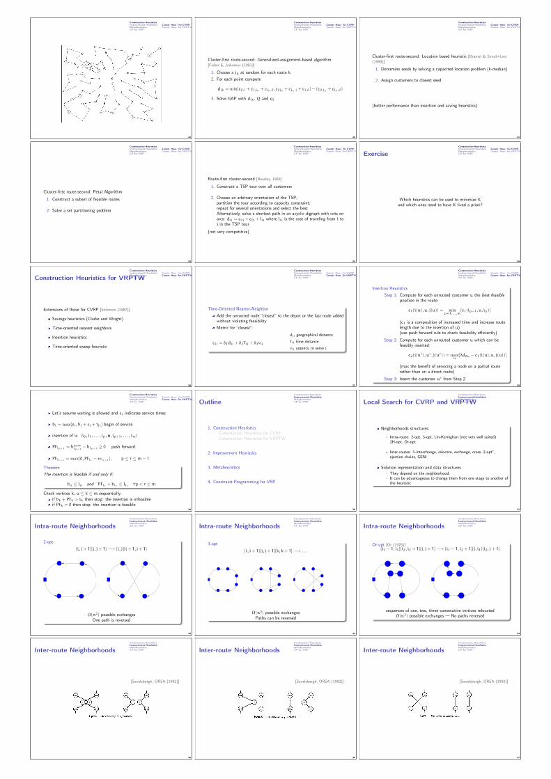
Construction HeuristicsImprovement HeuristicsMetaheuristicsCP for VRP
Constr. Heur. for CVRPConstr. Heur. for VRPTW
19
Construction HeuristicsImprovement HeuristicsMetaheuristicsCP for VRP
Constr. Heur. for CVRPConstr. Heur. for VRPTW
Cluster-first route-second: Generalized-assignment-based algorithm[Fisher & Jaikumur (1981)]
1. Choose a jk at random for each route k2. For each point compute
dik = minc0,i + ci,jk+ cjk,0, c0jk
+ cjk,i + ci,0 − (c0,jk+ cjk,0)
3. Solve GAP with dik, Q and qi
20
Construction HeuristicsImprovement HeuristicsMetaheuristicsCP for VRP
Constr. Heur. for CVRPConstr. Heur. for VRPTW
Cluster-first route-second: Location based heuristic [Bramel & Simchi-Levi(1995)]
1. Determine seeds by solving a capacited location problem (k-median)
2. Assign customers to closest seed
(better performance than insertion and saving heuristics)
21
Construction HeuristicsImprovement HeuristicsMetaheuristicsCP for VRP
Constr. Heur. for CVRPConstr. Heur. for VRPTW
Cluster-first route-second: Petal Algorithm
1. Construct a subset of feasible routes
2. Solve a set partitioning problem
22
Construction HeuristicsImprovement HeuristicsMetaheuristicsCP for VRP
Constr. Heur. for CVRPConstr. Heur. for VRPTW
Route-first cluster-second [Beasley, 1983]
1. Construct a TSP tour over all customers
2. Choose an arbitrary orientation of the TSP;partition the tour according to capacity constraint;repeat for several orientations and select the bestAlternatively, solve a shortest path in an acyclic digraph with cots onarcs: dij = c0i + c0j + lij where lij is the cost of traveling from i toj in the TSP tour.
(not very competitive)
23
Construction HeuristicsImprovement HeuristicsMetaheuristicsCP for VRP
Constr. Heur. for CVRPConstr. Heur. for VRPTWExercise
Which heuristics can be used to minimize Kand which ones need to have K fixed a priori?
24
Construction HeuristicsImprovement HeuristicsMetaheuristicsCP for VRP
Constr. Heur. for CVRPConstr. Heur. for VRPTWConstruction Heuristics for VRPTW
Extensions of those for CVRP [Solomon (1987)]
Savings heuristics (Clarke and Wright)
Time-oriented nearest neighbors
Insertion heuristics
Time-oriented sweep heuristic
26
Construction HeuristicsImprovement HeuristicsMetaheuristicsCP for VRP
Constr. Heur. for CVRPConstr. Heur. for VRPTW
Time-Oriented Nearest-Neighbor
Add the unrouted node “closest” to the depot or the last node addedwithout violating feasibilityMetric for “closest”:
cij = δ1dij + δ2Tij + δ3vij
dij geographical distance
Tij time distance
vij urgency to serve j
27
Construction HeuristicsImprovement HeuristicsMetaheuristicsCP for VRP
Constr. Heur. for CVRPConstr. Heur. for VRPTW
Insertion HeuristicsStep 1: Compute for each unrouted costumer u the best feasible
position in the route:
c1(i(u), u, j(u)) = minp=1,...,m
c1(ip−1, u, ip)
(c1 is a composition of increased time and increase routelength due to the insertion of u)(use push forward rule to check feasibility efficiently)
Step 2: Compute for each unrouted customer u which can befeasibly inserted:
c2(i(u∗), u∗, j(u∗)) = maxu
λd0u − c1(i(u), u, j(u))
(max the benefit of servicing a node on a partial routerather than on a direct route)
Step 3: Insert the customer u∗ from Step 228
Construction HeuristicsImprovement HeuristicsMetaheuristicsCP for VRP
Constr. Heur. for CVRPConstr. Heur. for VRPTW
Let’s assume waiting is allowed and si indicates service times
bi = maxei, bj + sj + tji begin of service
insertion of u: (i0, i1, . . . , ip,u, ip+1, . . . , im)
PFip+1= bnew
ip+1− bip+1
≥ 0 push forward
PFir+1= max0, PFir −wir+1
, p ≤ r ≤ m− 1
TheoremThe insertion is feasible if and only if:
bu ≤ lu and PFir + bir ≤ lir ∀p < r ≤ mCheck vertices k, u ≤ k ≤ m sequentially.
if bk + PFk > lk then stop: the insertion is infeasibleif PFk = 0 then stop: the insertion is feasible
29
Construction HeuristicsImprovement HeuristicsMetaheuristicsCP for VRPOutline
1. Construction HeuristicsConstruction Heuristics for CVRPConstruction Heuristics for VRPTW
2. Improvement Heuristics
3. Metaheuristics
4. Constraint Programming for VRP
30
Construction HeuristicsImprovement HeuristicsMetaheuristicsCP for VRPLocal Search for CVRP and VRPTW
Neighborhoods structures:
Intra-route: 2-opt, 3-opt, Lin-Kernighan (not very well suited)2H-opt, Or-opt
Inter-routes: λ-interchange, relocate, exchange, cross, 2-opt∗,ejection chains, GENI
Solution representation and data structuresThey depend on the neighborhood.It can be advantageous to change them from one stage to another ofthe heuristic
31
Construction HeuristicsImprovement HeuristicsMetaheuristicsCP for VRPIntra-route Neighborhoods
2-opt
i, i+ 1j, j+ 1 −→ i, ji+ 1, j+ 1
i i+1
jj+1
i i+1
jj+1
O(n2) possible exchangesOne path is reversed
32
Construction HeuristicsImprovement HeuristicsMetaheuristicsCP for VRPIntra-route Neighborhoods
3-opt
i, i+ 1j, j+ 1k, k+ 1 −→ . . .
i i+1
kk+1
j
j+1
i i+1
kk+1
j
j+1
i i+1
kk+1
j
j+1
O(n3) possible exchangesPaths can be reversed
33
Construction HeuristicsImprovement HeuristicsMetaheuristicsCP for VRPIntra-route Neighborhoods
Or-opt [Or (1976)]i1 − 1, i1i2, i2 + 1j, j+ 1 −→ i1 − 1, i2 + 1j, i1i2, j+ 1
jj+1
i −11 i +1
i 21
2
i
jj+1
i −11 i +1
i 21
2
i
sequences of one, two, three consecutive vertices relocatedO(n2) possible exchanges — No paths reversed
34
Construction HeuristicsImprovement HeuristicsMetaheuristicsCP for VRPInter-route Neighborhoods
[Savelsbergh, ORSA (1992)]
35
Construction HeuristicsImprovement HeuristicsMetaheuristicsCP for VRPInter-route Neighborhoods
[Savelsbergh, ORSA (1992)]
36
Construction HeuristicsImprovement HeuristicsMetaheuristicsCP for VRPInter-route Neighborhoods
[Savelsbergh, ORSA (1992)]
37

Inter-route Neighborhoods
GENI: generalized insertion [Gendreau, Hertz, Laporte, Oper. Res. (1992)]
select the insertion restricted to the neighborhood of the vertex tobe added (not necessarily between consecutive vertices)perform the best 3- or 4-opt restricted to reconnecting arc links thatare close to one another.
Construction HeuristicsImprovement HeuristicsMetaheuristicsCP for VRPEfficient Implementation
Intra-route
Time windows: Feasibility check
In TSP verifying k-optimality requires O(nk) timeIn TSPTW feasibility has to be tested then O(nk+1) time
(Savelsbergh 1985) shows how to verify constraints in constant timeSearch strategy + Global variables
⇓O(nk) for k-optimality in TSPTW
39
Construction HeuristicsImprovement HeuristicsMetaheuristicsCP for VRP
Search Strategy
Lexicographic search, for 2-exchange:i = 1, 2, . . . , n− 2 (outer loop)j = i+ 2, i+ 3, . . . , n (inner loop)
1
2
3
4
5
1,23,4−>1,32,41
2
3
4
5
1,24,5−>1,42,51
2
3
4
5
Previous path is expanded by the edge j− 1, j
40
Construction HeuristicsImprovement HeuristicsMetaheuristicsCP for VRP
Global variables (auxiliary data structure)
Maintain auxiliary data such that it is possible to:
handle single move in constant time
update their values in constant time
Ex.: in case of time windows:
total travel time of a path
earliest departure time of a path
latest arrival time of a path
41
Construction HeuristicsImprovement HeuristicsMetaheuristicsCP for VRPOutline
1. Construction HeuristicsConstruction Heuristics for CVRPConstruction Heuristics for VRPTW
2. Improvement Heuristics
3. Metaheuristics
4. Constraint Programming for VRP
42
Construction HeuristicsImprovement HeuristicsMetaheuristicsCP for VRPMetaheuristics
Many and fancy examples, but first thing to try:
Variable Neighborhood Search + Iterated greedy
43
Construction HeuristicsImprovement HeuristicsMetaheuristicsCP for VRP
Basic Variable Neighborhood Descent (BVND)
Procedure VNDinput : Nk, k = 1, 2, . . . , kmax, and an initial solution soutput: a local optimum s for Nk, k = 1, 2, . . . , kmax
k← 1
repeats ′ ← FindBestNeighbor(s,Nk)if g(s ′) < g(s) then
s← s ′
(k← 1)else
k← k+ 1
until k = kmax ;
44
Construction HeuristicsImprovement HeuristicsMetaheuristicsCP for VRP
Variable Neighborhood Descent (VND)
Procedure VNDinput : Nk, k = 1, 2, . . . , kmax, and an initial solution soutput: a local optimum s for Nk, k = 1, 2, . . . , kmax
k← 1
repeats ′ ← IterativeImprovement(s,Nk)if g(s ′) < g(s) then
s← s ′
(k← 1)else
k← k+ 1
until k = kmax ;
45
Construction HeuristicsImprovement HeuristicsMetaheuristicsCP for VRP
Final solution is locally optimal w.r.t. all neighborhoods
First improvement may be applied instead of best improvement
Typically, order neighborhoods from smallest to largest
If iterative improvement algorithms IIk, k = 1, . . . , kmax
are available as black-box procedures:order black-boxesapply them in the given orderpossibly iterate starting from the first oneorder chosen by: solution quality and speed
46
General recommendation: use a combination of 2-opt∗ + or-opt [Potvin,Rousseau, (1995)]
However,
Designing a local search algorithm is an engineering process in whichlearnings from other courses in CS might become important.
It is important to make such algorithms as much efficient as possible.
Many choices are to be taken (search strategy, order, auxiliary datastructures, etc.) and they may interact with instance features. Oftena trade-off between examination cost and solution quality must bedecided.
The assessment is conducted through:analytical analysis (computational complexity)experimental analysis
Construction HeuristicsImprovement HeuristicsMetaheuristicsCP for VRPIterated Greedy
Key idea: use the VRP cosntruction heuristics
alternation of Construction and Deconstruction phasesan acceptance criterion decides whether the search continues fromthe new or from the old solution.
Iterated Greedy (IG):determine initial candidate solution swhile termination criterion is not satisfied do
r := sgreedily destruct part of sgreedily reconstruct the missing part of sapply subsidiary iterative improvement procedure (eg, VNS)based on acceptance criterion,
keep s or revert to s := r
49
Construction HeuristicsImprovement HeuristicsMetaheuristicsCP for VRP
In the literature, the overall heuristic idea received different names:
Removal and reinsertion
Ruin and repair
Iterated greedy
Fix and re-optimize
50
Construction HeuristicsImprovement HeuristicsMetaheuristicsCP for VRP
RemoveRemove some related customers(their re-insertion is likely to change something)
Relatedness measure rij
geographical
rij =1
D(d ′(i, j) + d ′(i, j+ n) + d ′(i+ n, j) + d ′(i+ n, j+ n))
temporal and load based
d ′(u, v) = |Tpi− Tpj
| + |Tdi− Tdj
| + |li − lj|
cluster removal
history based: neighborhood graph removal
51
Construction HeuristicsImprovement HeuristicsMetaheuristicsCP for VRP
Dispersion sub-problem:choose q customers to remove with minimal rij
Heuristic stochastic procedure:
choose a pair randomly;select an already removed i and find j that minimizes rij
52
Construction HeuristicsImprovement HeuristicsMetaheuristicsCP for VRP
Insertion procedures:
Greedy (cheapest insertion)
Max regret:
∆fqi due to insert i into its best position in its qth best route
i = arg max(∆f2i − ∆f1i )
Constraint Programming (max 20 costumers)
53
Construction HeuristicsImprovement HeuristicsMetaheuristicsCP for VRP
Advantages of removal-reinsert procedure with many side constraints:
the search space in local search may become disconnected
it is easier to implement feasibility checks
no need of computing delta functions in the objective function
54
Construction HeuristicsImprovement HeuristicsMetaheuristicsCP for VRP
Further ideas
Adaptive removal: start by removing 1 pair and increase after acertain number of iterations
use of roulette wheel to decide which removal and reinsertionheuristic to use
pi =πi∑πi
for each heuristic i
SA as accepting criterion after each reconstruction
55

Construction HeuristicsImprovement HeuristicsMetaheuristicsCP for VRPOutline
1. Construction HeuristicsConstruction Heuristics for CVRPConstruction Heuristics for VRPTW
2. Improvement Heuristics
3. Metaheuristics
4. Constraint Programming for VRP
56
Construction HeuristicsImprovement HeuristicsMetaheuristicsCP for VRPPerformance of exact methods
Current limits of exact methods [Ropke, Pisinger (2007)]:
CVRP: up to 135 customers by branch and cut and price
VRPTW: 50 customers (but 1000 customers can be solved if theinstance has some structure)
CP can handle easily side constraints but hardly solve VRPs with morethan 30 customers.
57
Construction HeuristicsImprovement HeuristicsMetaheuristicsCP for VRPLarge Neighborhood Search
Other approach with CP: [Shaw, 1998]
Use an over all local search scheme
Moves change a large portion of the solution
CP system is used in the exploration of such moves.
CP used to check the validity of moves and determine the values ofconstrained variables
As a part of checking, constraint propagation takes place. Later,iterative improvement can take advantage of the reduced domains tospeed up search by performing fast legality checks.
58
Construction HeuristicsImprovement HeuristicsMetaheuristicsCP for VRP
Solution representation:
Handled by local search:Next pointers: A variable ni for every customer i representing thenext visit performed by the same vehicle
ni ∈ N ∪ S ∪ E
where S =⋃Sk and E =
⋃Ek are additional visits for each vehicle
k marking the start and the end of the route for vehicle k
Handled by the CP system: time and capacity variables.
59
Construction HeuristicsImprovement HeuristicsMetaheuristicsCP for VRP
Insertionby CP:
constraint propagation rules: time windows, load and boundconsiderations
search heuristic most constrained variable + least constrained valued(for each v find cheapest insertion and choose v with largest suchcost)
Complete search: ok for 15 visits (25 for VRPTW) but with heavytails
Limited discrepancy search
60
Construction HeuristicsImprovement HeuristicsMetaheuristicsCP for VRP
[Shaw, 1998]
61

DMP204SCHEDULING,
TIMETABLING AND ROUTING
Lecture 28
Rich Vehicle Routing Problems
Marco Chiarandini
A Uniform ModelOther Variants of VRPOutline
1. A Uniform Model
2. Other Variants of VRP
2
A Uniform ModelOther Variants of VRPOutline
1. A Uniform Model
2. Other Variants of VRP
3
A Uniform ModelOther Variants of VRPEfficient Local Search
Blackboard [Irnich 2008].
4
A Uniform ModelOther Variants of VRPOutline
1. A Uniform Model
2. Other Variants of VRP
5
A Uniform ModelOther Variants of VRPRich VRP
DefinitionRich Models are non idealized models that represetn the appliucation athand in an adequate way by including all important optimization criteria,constraints and preferences [Hasle et al., 2006]
Solution
Exact methods are often impractical:
instancs are too large
decision support systems require short response times
Metaheuristics based on local search components are mostly used
6
A Uniform ModelOther Variants of VRPVRP with Backhauls
Further Input from CVRP:a partition of customers:L = 1, . . . , n Lineahaul customers (deliveries)B = n + 1, . . . , n + m Backhaul customers (collections)precedence constraint:in a route, customers from L must be served before customers fromB
Task: Find a collection of K simple circuits with minimum costs, suchthat:
each circuit visit the depot vertexeach customer vertex is visited by exactly one circuit; andthe sum of the demands of the vertices visited by a circuit does notexceed the vehicle capacity Q.in any circuit all the linehaul customers precede the backhaulcustomers, if any.
7
A Uniform ModelOther Variants of VRPVRP with Pickup and Delivery
Further Input from CVRP:each customer i is associated with quantities di and pi to bedelivered and picked up, resp.for each customer i, Oi denotes the vertex that is the origin of thedelivery demand and Di denotes the vertex that is the destination ofthe pickup demand
Task:Find a collection of K simple circuits with minimum costs, such that:
each circuit visit the depot vertexeach customer vertex is visited by exactly one circuit; andthe current load of the vehicle along the circuit must benon-negative and may never exceed Q
for each customer i, the customer Oi when different from the depot,must be served in the same circuit and before customer i
for each customer i, the customer Di when different from the depot,must be served in the same circuit and after customer i
8
A Uniform ModelOther Variants of VRPMultiple Depots VRP
Further Input from CVRP:multiple depots to which customers can be assigneda fleet of vehicles at each depot
Task:Find a collection of K simple circuits for each depot with minimum costs,such that:
each circuit visit the depot vertexeach customer vertex is visited by exactly one circuit; andthe current load of the vehicle along the circuit must benon-negative and may never exceed Q
vehicles start and return to the depots they belongVertex set V = 1, 2, . . . , n and V0 = n + 1, . . . , n + m
Route i defined by Ri = l, 1, . . . , l
9
A Uniform ModelOther Variants of VRPPeriodic VRP
Further Input from CVRP:planning period of M days
Task:Find a collection of K simple circuits with minimum costs, such that:
each circuit visit the depot vertexeach customer vertex is visited by exactly one circuit; andthe current load of the vehicle along the circuit must benon-negative and may never exceed Q
A vehicle may not return to the depot in the same day it departs.Over the M-day period, each customer must be visited l times,where 1 ≤ l ≤ M.
10
A Uniform ModelOther Variants of VRP
Three phase approach:1. Generate feasible alternatives for each customer.
Example, M = 3 days d1, d2, d3 then the possible combinationsare: 0 → 000; 1 → 001; 2 → 010; 3 → 011; 4 → 100; 5 → 101;6 → 110; 7 → 111.Customer Diary De-
mandNumber ofVisits
Number ofCombina-tions
PossibleCombina-tions
1 30 1 3 1,2,42 20 2 3 3,4,63 20 2 3 3,4,64 30 2 3 1,2,45 10 3 1 7
2. Select one of the alternatives for each customer, so that the dailyconstraints are satisfied. Thus, select the customers to be visited ineach day.
3. Solve the vehicle routing problem for each day.
11
A Uniform ModelOther Variants of VRPSplit Delivery VRP
Constraint Relaxation: it is allowed to serve the same customer bydifferent vehicles. (necessary if di > Q)
Task:Find a collection of K simple circuits with minimum costs, such that:
each circuit visit the depot vertexthe current load of the vehicle along the circuit must benon-negative and may never exceed Q
Note: a SDVRP can be transformed into a VRP by splitting eachcustomer order into a number of smaller indivisible orders [Burrows 1988].
12
A Uniform ModelOther Variants of VRPInventory VRP
Input:a facility, a set of customers and a planning horizon T
ri product consumption rate of customer i (volume per day)
Ci maximum local inventory of the product for customer i
a fleet of M homogeneous vehicles with capacity Q
Task:Find a collection of K daily circuits to run over the planing horizon withminimum costs and such that:
each circuit visit the depot vertexno customer goes in stock-out during the planning horizonthe current load of the vehicle along the circuit must benon-negative and may never exceed Q
13
A Uniform ModelOther Variants of VRPOther VRPs
VRP with Satellite Facilities (VRPSF)
Possible use of satellite facilities to replenish vehicles during a route.
Open VRP (OVRP)
The vehicles do not need to return at the depot, hence routes are notcircuits but paths
Dial-a-ride VRP (DARP)
It generalizes the VRPTW and VRP with Pick-up and Delivery byincorporating time windows and maximum ride time constraints
It has a human perspective
Vehicle capacity is normally constraining in the DARP whereas it isoften redundant in PDVRP applications (collection and delivery ofletters and small parcels)
14