Introduction to Benchmarks

Introduction to Benchmarks

by C. Mitchell Conover, PhD, CFA, CIPM, Daniel Broby, FSIP, and David R. Cariño, PhD

LEARNING OUTCOMES

Mastery The candidate should be able to:

a. define the term “benchmark” and distinguish between benchmarks and

market indexes;

b. describe how benchmarks are used in return attribution and

performance appraisal;

c. distinguish among types of benchmarks;

d. explain desirable properties of benchmarks in the context of performance

attribution;

e. explain a portfolio’s positions in terms of a market index’s security

positions, benchmark positions, style tilts, and active positions;

f. identify and explain tests of benchmark quality;

g. compare the theoretical advantages and disadvantages, data

requirements, and costs of using each type of benchmark;

h. interpret peer universe box charts;

i. explain uses of asset class indexes;

j. compare market- capitalization- weighting, equal- weighting, price-

weighting, and fundamental- weighting index construction schemes,

including their advantages and disadvantages;

k. describe the purpose and effects of float adjustment of market

capitalization indexes;

l. explain the tradeoffs in constructing asset class indexes;

m. describe classifications of equity investing styles and the construction of

associated equity style indexes;

n. explain bond market sectors and the construction of associated bond

style indexes;

o. describe the steps in constructing a (security- based) custom benchmark;

p. describe the impact of benchmark misspecification on attribution and

appraisal analysis;

q. recommend and justify the choice of a benchmark for a portfolio given a

description of portfolio objectives and management processes.

R E A D I N G

6

Copyright © 2013 CFA Institute

Reading 6 ■ Introduction to Benchmarks362

INTRODUCTION

The Oxford English Dictionary defines a benchmark as “a standard or point of reference against

which things may be compared.” In an investments context, a benchmark is a standard or point

of reference for evaluating the performance of an investment portfolio. The selection of an

appropriate benchmark depends on the objective and constraints that govern the construction

of the portfolio.

An investment benchmark is typically a collection of securities that characterizes a manag-

er’s preferred habitat of securities and risk. For example, an investor in German equities with

characteristically small market capitalizations (and no other distinctive selection character-

istics) might have a benchmark consisting of a broad portfolio of small- market- cap German

equities. However, a benchmark can also be a market rate of return—for example, when the

investment strategy targets achieving a specific rate of return and the strategy cannot be readily

represented by a portfolio.

Benchmarks make it possible to determine how effectively active fund managers—managers

who trade on perceived opportunities to earn superior risk- adjusted returns—have performed

by measuring the impact of decisions to depart from benchmark weights. An ideal benchmark

provides the portfolio manager and his or her investment clients with an objective means of

evaluating how skillfully the manager implemented his or her investment strategy. Analysts can

use it when attempting to identify active investment management skill. Well- chosen benchmarks

allow returns to be accurately evaluated and decomposed. If the benchmark chosen is invalid,

then all subsequent portfolio manager evaluation and analysis is incorrect.1 Throughout this

reading, we refer to the ideal benchmark as one that is “valid,” consistent with the literature

in the field. Although a valid benchmark may not be attainable in certain circumstances, the

goal of a performance analyst should be to use a benchmark that allows the most accurate

evaluation of manager performance.

The importance of benchmarks to owners of capital cannot be underestimated. Benchmarks

communicate information about an investment manager’s investment universe (the set of assets

that may be considered for investment) and investment discipline. Investment managers often

claim to beat the “market.” The benchmark defines what the relevant “market” is and allows an

analysis of the manager’s performance.

Benchmarks provide investment managers with a guidepost for acceptable levels of risk

and return. They can be a powerful influence on investment decision making. As one invest-

ment authority has opined, “Benchmarks determine the performance of investment managers

perhaps more than any other influence, including managers’ determination to succeed and

the resources and skills they bring to this task. We in the industry have largely overlooked this

fact, perhaps at our peril.”2

This reading will help the reader understand benchmarks. Among the questions it will

answer are the following:

■ How are benchmarks used?

■ What are the properties of a valid benchmark, and how can they be tested for quality?

■ What are the various types of benchmarks, and what are their advantages and

disadvantages?

■ How are indexes constructed?

■ How are custom benchmarks constructed?

■ What are some alternative benchmarks?

■ What is the impact of poorly specified benchmarks on investment analysis?

The rest of the reading is organized as follows. Section 2 clarifies the distinction between

two terms important in the discussion, benchmark and market index. Section 3 provides an

overview of benchmarks and discusses how they are used, their types, their desirable proper-

ties, and how their quality can be ascertained. Section 4 discusses the use of peer groups as

1

1 A humorous analogy is provided by Surz (2009, p. 140). Using an invalid benchmark to determine skill

is like evaluating Tiger Woods as a bowler.

2 Siegel (2003, p. ix).

Benchmarks in Performance Attribution and Appraisal: Overview 363

benchmarks, Section 5 examines market indexes and style benchmarks, Section 6 introduces

custom benchmarks, and Section 7 explores the use of factor- model- based benchmarks. Each

of these sections assesses the advantages and disadvantages of the various benchmarks. Section

8, on alternative benchmarks, examines returns- based, hedge fund, and liability- based bench-

marks. Section 9 describes problems with benchmark misspecification. The reading concludes

with Section 10.

DISTINGUISHING BETWEEN A BENCHMARK AND A

MARKET INDEX

Although the terms “benchmark” and “market index” (or simply “index”) are often loosely used

interchangeably, we must distinguish between them to have an accurate discussion. A market

index represents the performance of a specified security market, market segment, or asset class.

For example, the FTSE 100 Index is an index constructed to represent the broad performance of

large- cap UK equities. The Barclays Sterling Aggregate Bond Index represents the performance

of fixed- rate, investment- grade sterling- denominated bonds; in contrast, the Barclays Sterling

Gilts Index captures the performance of a narrower segment of the UK investment- grade debt

market—UK government debt. The constituents of each of these indexes are selected for their

appropriateness in representing the targeted market, market segment, or asset class. A market

index may be considered for use as a benchmark or comparison point for an investment manager;

however, the most appropriate benchmark or reference point for an investment manager need

not be an available market index. A good example in which a market index is an appropriate

benchmark is the case of passive managers, who typically invest in a portfolio similar (or iden-

tical) to a chosen market index so as to closely track its performance. For example, the iShares

Core S&P 500 ETF (exchange- traded fund), ticker IVV, seeks investment results, before fees

and expenses, that correspond to the price and yield performance of US large- cap stocks as

represented by the S&P 500 Index. Because the investment objective of the IVV is to track the

performance of the S&P 500, the S&P 500 is the appropriate benchmark for IVV, as it is for

any other investment with an identical investment objective. An active US core equity manager

whose investment universe is the S&P 500—that is, one that seeks to add value by under- or

overweighting component securities of the S&P 500—and no other securities and that has no

observable selection biases might also use the S&P 500 as its benchmark. However, another

active manager might not follow an investment discipline for which an existing security market

index is a valid reference point. Market indexes are typically meant to serve the general public’s

purposes and to have broad appeal. Benchmarks must be appropriate for the specific investor

(sponsor) and any investment manager hired to manage money.3 The fundamental requirements

of indexes and valid benchmarks are formulated differently, as we will explain subsequently.

Nevertheless, because market indexes can often serve as valid benchmarks (according to the

facts of the case), performance analysts should become knowledgeable about market indexes.

The reader will find that writers and index vendors vary in their preference for the plural

of “index.” For simplicity, throughout this reading we will consistently use “indexes” rather than

the Latin- inspired “indices” as the plural of “index.”

BENCHMARKS IN PERFORMANCE ATTRIBUTION AND

APPRAISAL: OVERVIEW

This section gives a general overview of benchmarks, including their uses, their types, their

desirable properties, and tests of benchmark quality. The context of the discussion could equally

be taken to be private wealth management or institutional portfolio management. Much of the

theory was developed in the institutional world.

2

3

3 Amenc, Goltz, and Tang (2011, p. 68).


A plan sponsor is the trustee, company, or employer that is responsible for a public or

private institutional investment plan. The responsibilities of the plan sponsor include determin-

ing membership parameters, investment choices, contributions, and distributions. The type of

benchmark chosen will differ depending on its characteristics. In a private wealth context, we

would be referring in general to the investor.

A fund manager is the professional manager of separate accounts or pooled assets structured

in any of a variety of ways (e.g., a US mutual fund, a UK unit trust, a European Union UCITS

fund, an exchange- traded fund, or a hedge fund). Although the plan sponsor could manage a

fund in house, in general, we will think of the fund manager as an external investment manager

to whom management of a part of the sponsor’s assets is delegated. The fund manager may

have a mandate from the sponsor to follow either a passive or an active investment strategy.

■ Passive investment strategies prominently include indexing.4 Indexers seek to deliver

investment returns comparable to those of a market index by investing in or replicating

the index constituents.

■ Active investment strategies seek to use a fund manager’s insight to deliver invest-

ment returns in excess of those from a passive buy- and- hold strategy. These returns are

referred to as the manager’s active returns, and the variability of the active returns is

referred to as active risk.

Benchmarks are vital for performance measurement when the assets are actively man-

aged. However, benchmarks are also relevant when passive investment strategies are used, as

discussed below.

3.1 Benchmarks: Investment Uses

There are several uses of benchmarks in investment practice. These include

■ reference points for segments of the sponsor’s portfolio;

■ communication of instructions to the manager;

■ communication of instructions to a board of directors (or any oversight group) and

consultants;

■ identification and evaluation of current portfolio’s risk exposures;

■ interpretation of past performance and performance attribution;

■ manager selection and appraisal;

■ marketing of investment products; and

■ demonstration of compliance with regulations, laws, or standards.

Sponsor benchmarks need to be distinguished from fund manager benchmarks. A sponsor’s

strategic asset allocation (policy portfolio) is the long- run allocation to asset classes consistent

with the investor’s objectives and constraints. From this, a benchmark, often in the form of an

investable market index, will be specified for each asset class in the strategic asset allocation.

That practice implicitly and reasonably specifies a passive investment in the asset class as a

neutral comparison point in measuring sponsor progress toward investment goals.

In general when we refer simply to benchmarks, the reference will be to benchmarks pro-

vided to fund managers that are appropriate references for their specific investment disciplines.

Given the sponsor’s understanding of the fund manager’s investment discipline, the benchmark

conveys the sponsor’s expectations to the manager as to how the fund assets will be invested and

their expected risk and return. By conveying the sponsor’s expectations, benchmarks provide

accountability, so that if a manager’s security selection and subsequent performance frequently

diverges far from the benchmark, it is apparent that the manager’s investment approach is

inconsistent with the fund’s stated investment discipline. Benchmarks also ensure a degree of

fairness in the sense that the manager will not be held to standards that the fund’s board or

consultants might arbitrarily impose.

4 “Buy and hold” is another example of a passive strategy. However, indexing is by far the most important

passive investment strategy in terms of assets committed to it and the only one discussed in this reading.


Second, the benchmark communicates to the board and external consultants the manag-

er’s area of expertise and how a manager should subsequently invest and be evaluated. In a

multiple- manager fund, benchmarks convey the managers’ coverage areas, so that assets and

securities that lack coverage or are overemphasized can be identified.

A third use of benchmarks is to identify and evaluate the risk exposures of the manager.

Managers often describe themselves as “value managers” or “growth managers.” However, these

terms are imprecise. An appropriate benchmark will have risk similar to the portfolio and be

informative in revealing the manager’s active risk exposures, which should help explain the

manager’s performance within his or her chosen investment style.

Another fundamental use of benchmarks is to attribute and appraise past performance and,

in general, the consequences of the manager’s investment decisions. The benchmark helps the

board and its consultants determine and evaluate the manager’s excess return (the difference

between the portfolio return and the benchmark return, which may be either positive or neg-

ative). Return attribution identifies such things as whether the manager’s security selection,

industry bets (in equity analysis), or yield curve positioning (in fixed- income analysis) have

added value. What caused the manager’s performance to be different from the benchmark’s?

Performance appraisal’s chief focus is to distinguish active investment skill from luck.

Accounting or adjusting for risk may be accomplished in a variety of ways. One appraisal

tool known as the information ratio (IR) attempts to measure the value added per unit of active

risk. To calculate IR, the mean portfolio return in excess of the benchmark return is divided

by the active risk.5 If the benchmark is inappropriate, the calculated value of IR will not be

informative. Thus, when benchmarks are used in performance appraisal, benchmark selection

is obviously important.

Inappropriate benchmarks introduce noise into the investment manager assessment process

and provide a misleading picture of manager performance. Good benchmarks enhance the

effectiveness of manager assessment, whereas bad ones may lead to an inefficient or unintended

allocation of fund assets and disguise managers’ contributions.6 As a result, benchmarks will

also be instrumental in investment contracts that have an incentive compensation component

in which outperformance is rewarded (and underperformance is possibly penalized).

Furthermore, benchmarks play a role in the manager selection processes because they

will influence the perception of a manager’s skill. The analysis of past performance will involve

a qualitative assessment of whether the manager’s investment process is robust enough to

produce repeatable outperformance in the future or, alternatively, whether a manager’s past

underperformance is likely to persist.

Benchmarks are also used to market investment products to potential investors. The

Global Investment Performance Standards (GIPS®) require that if a benchmark exists, it must

be included in a performance presentation with its description. If no benchmark is provided,

a reason must be given. Marketing requires the communication and explanation of the invest-

ment process, of which the benchmark is an essential descriptor of the investment strategy

and a crucial determinant of excess returns. Excess returns have been found to be a significant

determinant of investor inflows, so the choice of the benchmark will influence the fund’s ability

to attract new capital.

Lastly, benchmarks are used to demonstrate compliance with regulations, laws, and standards.

Regulatory organizations use benchmarks as part of their oversight and surveillance, and as a

result, benchmarks have become mandated in many jurisdictions. In 1998, the US SEC intro-

duced a requirement that mutual funds self- designate a benchmark and present their historical

returns alongside it in the prospectus. Many other jurisdictions now have similar rules. More

generally, institutions are sometimes restricted from investing in specific instruments, such as

below- investment- grade bonds. Benchmarks for such institutions have to be tailored accordingly.

5 This is the common definition used in industry. The numerator in the IR is most precisely defined as

alpha, the excess return after completely adjusting for risk. If the risk of the portfolio and the benchmark are

exactly the same (the beta of the portfolio with respect to the benchmark equals 1), the two are equivalent.

6 “Inefficient” is used in an investment context here, referring to an asset allocation that does not have

an optimal risk–return tradeoff.


3.2 Types of Benchmarks

Given the uses described above, benchmarks are an important part of the investment process

for both institutional and private wealth clients. In the discussion below, we introduce the types

of benchmarks based on the discussion in Bailey, Richards, and Tierney (2007).7 The seven

benchmarks introduced in this section are

■ absolute (including target) return benchmarks;

■ manager universes (peer groups);

■ broad market indexes;

■ style indexes;

■ factor- model- based benchmarks;

■ returns- based (Sharpe style analysis) benchmarks; and

■ custom security- based (strategy).

An absolute return benchmark is simply a minimum target return that the manager is

expected to beat. The return may be a stated minimum (e.g., 9%), stated as a spread above a

market index (e.g., euro interbank offered rate + 4%), or determined from actuarial assumptions.

An example of an absolute return benchmark is 30% per annum return for a private equity

investment (e.g., a buyout fund—note that more sophisticated benchmarks are available).

Market neutral long‒short equity funds are another example of a type of fund sometimes given

an absolute return benchmark. Such funds are run by portfolio managers who believe that they

can identify over- and undervalued shares. Such a fund consists of long and short positions

in, respectively, perceived undervalued and overvalued equities and is constructed so that,

overall, the portfolio is expected to be insensitive to broad equity market movements—that

is, market neutral with a market beta of zero. Because a market neutral fund is in principle a

zero–expected systematic risk investment, the benchmark may be specified as a three- month

Treasury bill return; the investment objective may be to outperform the benchmark consistently

by a given number of basis points.

A manager universe—or manager peer group—is a broad group of managers with similar

investment disciplines. Manager universe benchmarks allow investors to make comparisons

with the performance of other managers following similar investment disciplines. Managers are

typically expected to beat the median manager return, which refers to the manager return that

splits the sample of managers’ returns in half. Manager universes are typically formed by asset

class and the investment approach within that class. Hedge funds have often been evaluated

relative to manager universe benchmarks provided by such vendors as Credit Suisse/Tremont,

Hedge Fund Research, and Lipper/TASS. Private equity funds are also commonly evaluated in

this way; examples of data vendors are Burgiss, Cambridge Associates, Preqin, and Thomson

Venture Economics. Investment magazines are prolific providers of peer group comparisons

for investment funds (e.g., mutual funds in the United States and unit trusts in the United

Kingdom); thus, a mutual fund investing in global equities might be ranked among all mutual

funds with similar objectives over various time periods.

Broad market indexes are measures of broad asset class performance, such as the JP Morgan

Emerging Markets Bond Index (EMBI) for emerging market bonds or the MSCI World Index

for global developed market equities. Broad market indexes are well known, readily available,

and easily understood. The number of market indexes has proliferated over time so as to serve

a greater number and variety of applications and end users. For example, in 1999, JP Morgan

created the EMBI Global index (EMBIG), which added less liquid issues and less creditworthy

issues to the EMBI. The performance of broad market indexes is widely reported in popular

media, such as television.

Market indexes have also been more narrowly defined to represent investment styles within

asset classes, resulting in style indexes. (An investment style can be defined as a natural

grouping of investment disciplines that has some predictive power in explaining the future

dispersion of returns across portfolios.)8 In the late 1970s, researchers found that stock valua-

tion (e.g., defined using the price- to- earnings ratio) and market capitalization explained much

7 More detailed discussion for each benchmark is provided in the remainder of the reading.

8 See Brown and Goetzmann (1997).


of stock return variation. In response, many index providers provided various style versions

of their broad market indexes. For example, in 1999, Wilshire introduced value, growth, and

size subsets of its US Wilshire 5000 Index.9 Style indexes are formed under the belief that a

characteristic of an asset, such as a stock’s dividend yield or a bond’s credit rating, will be the

primary determinant of its subsequent performance.

Factor- model- based benchmarks are constructed by examining the portfolio’s sensitivity

to a set of factors. Examples of factors include the return for a broad market index, company

earnings growth, industry, and financial leverage. The simplest form of a factor- model- based

benchmark is the market model, in which there is a single factor, the return on a broad market

index. To determine the factor sensitivities, the portfolio’s return is regressed against the factors

believed to influence returns. The general form of a factor model is

Rp = ap + b1F1 + b2F2 … bkFk + εp

where

Rp = the portfolio’s periodic return

ap = the “zero- factor” term, which is the expected portfolio return if all factor sensitivi-

ties are zero

bk = the sensitivity of portfolio returns to the factor return

Fk = systematic factors responsible for asset returns

εp = residual return due to nonsystematic factors

The sensitivities (bk) are then used to predict the return the portfolio should provide for

given values of the systematic risk factors; a higher positive sensitivity indicates greater positive

exposure to a specified factor and higher expected return, holding all else equal. The factors

(F) represent values that are related to security values, such as interest rates. For example,

interest rates may be inversely related to security prices. If interest rates unexpectedly rise,

then security returns will fall by the amount determined by the security’s sensitivity (bk) to

interest rate changes.

Returns- based benchmarks (Sharpe style analysis) are similar to factor- model- based

benchmarks in that portfolio returns are related to a set of factors that do well in explaining

portfolio returns. In the case of returns- based benchmarks, however, the factors are the returns

for various style indexes (e.g., small- cap value, small- cap growth, large- cap value, and large- cap

growth). The analysis produces a benchmark that is essentially the weighted average of these

asset class indexes that best explains or tracks the portfolio’s returns. The difference between

the use of the style indexes previously discussed and returns- based benchmarks is that the latter

view style on a continuum; for example, a portfolio may be characterized as 60% small- cap value

and 40% small- cap growth. To create a returns- based benchmark using Sharpe style analysis,

an optimization procedure is used in which the portfolio’s sensitivities (analogous to the bk’s

in factor- model- based benchmarks) are forced to be non- negative and sum to 1.

Lastly, custom security- based benchmarks are custom built to accurately reflect the

investment discipline of a particular investment manager. Such benchmarks are developed

through discussions with the manager and an analysis of past portfolio exposures. After the

manager’s investment process is identified, the benchmark is constructed by selecting securi-

ties and weightings consistent with that process and client restrictions. A cash weight is also

identified that is appropriate for the situation. The benchmark is subsequently rebalanced on a

periodic basis to ensure that it stays consistent with the manager’s investment practice. Custom

security- based benchmarks are also referred to as strategy benchmarks because they should

reflect the manager’s particular strategy. Custom security- based benchmarks are particularly

appropriate when the manager’s strategy cannot be closely matched to a broad market index

or style index.

(1)

9 Broadly speaking, a value investment style with respect to equity portfolio management is focused on

paying a relatively low price with respect to earnings or assets per share. A growth investment style with

respect to equity portfolio management is focused on investing in high- earnings- growth companies. Section

5.3 examines style in more detail.


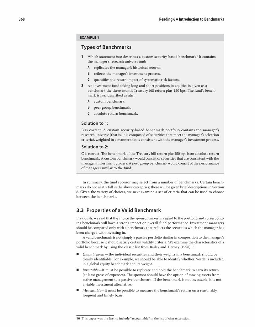
EXAMPLE 1

Types of Benchmarks

1 Which statement best describes a custom security- based benchmark? It contains

the manager’s research universe and:

A replicates the manager’s historical returns.

B reflects the manager’s investment process.

C quantifies the return impact of systematic risk factors.

2 An investment fund taking long and short positions in equities is given as a

benchmark the three- month Treasury bill return plus 150 bps. The fund’s bench-

mark is best described as a(n):

A custom benchmark.

B peer group benchmark.

C absolute return benchmark.

Solution to 1:

B is correct. A custom security- based benchmark portfolio contains the manager’s

research universe (that is, it is composed of securities that meet the manager’s selection

criteria), weighted in a manner that is consistent with the manager’s investment process.

Solution to 2:

C is correct. The benchmark of the Treasury bill return plus l50 bps is an absolute return

benchmark. A custom benchmark would consist of securities that are consistent with the

manager’s investment process. A peer group benchmark would consist of the performance

of managers similar to the fund.

In summary, the fund sponsor may select from a number of benchmarks. Certain bench-

marks do not neatly fall in the above categories; these will be given brief descriptions in Section

8. Given the variety of choices, we next examine a set of criteria that can be used to choose

between the benchmarks.

3.3 Properties of a Valid Benchmark

Previously, we said that the choice the sponsor makes in regard to the portfolio and correspond-

ing benchmark will have a strong impact on overall fund performance. Investment managers

should be compared only with a benchmark that reflects the securities which the manager has

been charged with investing in.

A valid benchmark is not simply a passive portfolio similar in composition to the manager’s

portfolio because it should satisfy certain validity criteria. We examine the characteristics of a

valid benchmark by using the classic list from Bailey and Tierney (1998).10

■ Unambiguous—The individual securities and their weights in a benchmark should be

clearly identifiable. For example, we should be able to identify whether Nestlé is included

in a global equity benchmark and its weight.

■ Investable—It must be possible to replicate and hold the benchmark to earn its return

(at least gross of expenses). The sponsor should have the option of moving assets from

active management to a passive benchmark. If the benchmark is not investable, it is not

a viable investment alternative.

■ Measurable—It must be possible to measure the benchmark’s return on a reasonably

frequent and timely basis.

10 This paper was the first to include “accountable” in the list of characteristics.


■ Appropriate—The benchmark must be consistent with the manager’s investment style or

area of expertise.

■ Reflective of current investment opinions—The manager should be familiar with the secu-

rities that constitute the benchmark and their factor exposures. The manager should be

able to develop an opinion regarding their attractiveness as investments; he should not

be given a mandate containing obscure securities that he could not be expected to have

knowledge of.

■ Specified in advance—The benchmark must be constructed prior to the evaluation

period so that the manager is not judged against benchmarks created after the fact.

■ Accountable—The manager should accept ownership of the benchmark and its securities

and be willing to be held accountable to the benchmark.

The benchmark should be fully consistent with the manager’s investment process, and the

manager should be able to demonstrate the validity of his or her benchmark. Through accep-

tance of the benchmark, the sponsor assumes responsibility for any discrepancies between

the targeted portfolio for the fund and the benchmark. The manager becomes responsible for

differences between the benchmark and her performance.

The properties outlined by Bailey and Tierney (1998) help ensure that a benchmark will

serve as a valid instrument for the purposes of evaluating the manager’s performance. Although

this list of qualities for a desirable benchmark may seem straightforward, we will show later

that many commonly used benchmarks do not incorporate them.

3.4 Evaluating Benchmark Quality: Analysis Based on a

Decomposition of Portfolio Holdings and Returns

Once a benchmark is constructed, we can evaluate its quality using tests. To understand these

tests, it helps to first decompose the benchmark’s returns. Using the decomposition from

Bailey, Richards, and Tierney (2007), we can first state the identity where a portfolio’s return

(P) is equal to itself:

P = P

Then, add and subtract an appropriate benchmark (B) from the right- hand side of the equation:

P = B + (P − B)

Defining the manager’s active management decisions (A) as the difference between the

portfolio and benchmark returns (P – B), we have

P = B + A

Here, we see that the manager’s return is a function of the benchmark return and the active

management decisions.

Next, add and subtract the market index return (M) from the right- hand side of the equation:

P = M + (B – M) + A

Defining the manager’s investment style (S) as the difference between the benchmark return

and the market index (B – M) results in

P = M + S + A

The final equation states that a manager’s portfolio return (P) is a result of the market index

return (M), style (S), and active management return (A).

If the manager’s portfolio is a broad market index, then S and A = 0 and, as expected,

the portfolio earns the broad market return: P = M. If the benchmark used is a broad market

index, then S is assumed to be zero, and the prediction is that the manager earns the market

return and a return to active management: P = M + A. However, when a broad market index

is used as a benchmark and the manager actually has style differences from it, the analysis and

its return prediction is incorrect. In this case, the manager’s style return (S) will be reflected

in the measured active management component (A), such that an analysis of a manager’s true

value added will be obscured.

(2)

(3)

(4)

(5)

(6)


EXAMPLE 2

Decomposition of Portfolio Return

In calculation questions, show final results to one decimal place.

1 Assume that the Courtland account has a return of –5.3% in a given month,

during which the portfolio benchmark has a return of –5.5% and the market index

has a return of –2.8%.

A Calculate the Courtland account’s return due to the manager’s style.

B Calculate the Courtland account’s return due to active management.

2 Assume that Mr. Kuti’s account has a return of 5.6% in a given month, during

which the portfolio benchmark has a return of 5.1% and a market index has a

return of 3.2%.

A Calculate the return due to the manager’s style for Mr. Kuti’s account.

B Calculate the return due to active management for Mr. Kuti’s account.

3 An actively managed midcap value equity portfolio has a return of 9.24%. The

portfolio is benchmarked to a midcap value index that has a return of 7.85%. A

broad equity market index has a return of 8.92%. Calculate the return due to the

portfolio manager’s style.

4 A US large- cap value portfolio run by Anderson Investment Management

returned 18.9% during the first three quarters of 2013. During the same time

period, a US large- cap value index had returns of 21.7% and a broad US equity

index returned 25.2%.

A Calculate the return due to style.

B Calculate the return due to active management.

C Describe the implications of your answers to Parts A and B for assessing

Anderson’s performance relative to the benchmark and relative to the market.

Solutions:

1 A The return due to style is S = B – M = –5.5% – (–2.8%) = –2.7%.

B The return due to active management is A = P – B = –5.3% – (–5.5%) = 0.2%.

2 A The return due to style is S = B – M = 5.1% – 3.2% = 1.9%.

B The return due to active management is A = P – B = 5.6% – 5.1% = 0.5%.

3 The return due to style is the style- specific benchmark return of 7.85% minus the

broad market return of 8.92%—that is, –1.07%.

4 A The return due to style is the difference between the benchmark and the mar-

ket index, or S = (B − M) = (21.7% − 25.2%) = −3.5%.

B The return due to active management is the difference between the portfolio

and the benchmark, or A = (P − B) = (18.9% − 21.7%) = −2.8%.

C The implication of the style calculation is that large- cap value was out of favor

in the period measured: That is, the US large- cap value index underperformed

the US market index by 3.5%.

The implication of the active management calculation is that Anderson is

not adding value compared with the benchmark because its portfolio under-

performed the portfolio benchmark. If Anderson is indeed a large- cap value

manager and the US large- cap value index is an appropriate benchmark, then

the client would have been better off investing in the passive alternative.


The analysis facilitates a discussion of tests of benchmark quality from Bailey (1992b) and

Bailey, Richards, and Tierney (2007). These tests are designed to reflect the previously discussed

properties of a valid benchmark and the various uses to which benchmarks are applied.11 Good

benchmarks should possess the following eight characteristics.

1 The correlation (ρ) between the manager’s active return and style return should be statis-

tically indistinguishable from zero.

ρA,S = 0

If Equation 7 holds, whether the manager’s style is in or out of favor should have no

effect on the manager’s ability to generate excess returns. Intuitively, if a benchmark fully

captures a manager’s investment process, the residual variability in the manager’s returns

should not be explainable by the index.

2 Defining E as the difference between the manager’s portfolio and a broad market index,

the correlation between E = (P – M) and the style return S = (B – M) should be positive:

ρE,S > 0

In other words, if the manager’s portfolio outperforms (underperforms) the broad mar-

ket, the tendency should be for the manager’s style to outperform (underperform) the

market. Stated differently, the investment styles of the benchmark and portfolio should

be similar if the benchmark is to explain a large proportion of the manager’s returns.12

3 The standard deviation of A = (P – B) should be less than the standard deviation of E =

(P – M):

σA < σE

In other words, the manager’s portfolio should more closely track the benchmark than

a market index. Stated differently, the tracking risk (i.e., the standard deviation) of (A =

P – B) should be lower than the tracking risk of (E = P – M). This condition indicates

that the benchmark is capturing important characteristics of the manager’s investment

process. If not, the evaluation of the manager’s performance will be contaminated by

noise introduced by a poor benchmark.13

4 Recall the previously discussed factor model (Equation 1) in which we examined the

portfolio’s and benchmark’s sensitivities (bk) to risk factors:


Good benchmarks will have portfolio and benchmark sensitivities that are similar over

time (i.e., of the same sign and comparable in magnitude). Although the risk sensitivities

will not be the same in a given period when the manager takes active bets, over time,

the benchmark should reflect the risk of the portfolio. Otherwise, systematic bias exists

between the benchmark and portfolio.

5 In the case of equities, the benchmark should exhibit low turnover, which is the propor-

tion of benchmark market value used for purchasing new securities when it is rebal-

anced. Low turnover means that the benchmark can be held as a passive investment (so

that it is investable). Bailey (1992b) estimated that turnover of 15%–20% per quarter

is acceptably low benchmark turnover.14 Fixed- income portfolios and benchmarks are

inherently subject to turnover because of redemptions, calls, and other events, and the

low turnover criterion is less clearly applicable to them.

(7)

(8)

(9)

11 Compared with Bailey (1992b), Criterion 7 has been modified to focus on equities.

12 These correlation requirements imply that the beta of the portfolio with respect to the benchmark is 1

and that, with respect to the market, the betas of the portfolio and benchmark will be similar. See Tierney

and Bailey (1995, pp. 28−29).

13 For a given level of excess return, a good benchmark will also have a higher information ratio than a

poor benchmark because of its lower tracking risk. See Bailey (1992a, p. 11).

14 His specification includes the reinvestment of income.


6 The benchmark should have investable position sizes, where its positions could be

replicated by the portfolio without excessive trading costs. For example, the amount a

benchmark holds in a small- capitalization stock should not exceed the tradeable value

that a manager could attain.

7 If the benchmark contains many securities that the manager has no opinion on or

that are inappropriate, then the manager will have a zero weight in those securities.

Therefore, a high proportion of zero portfolio weights in the benchmark’s securities may

be indicative of a benchmark that is poorly representative of a manager’s investment

approach. Further investigation would be needed to determine whether the zero weights

reflect an inappropriate benchmark or negative opinions of the manager.

8 Finally, there should be high coverage of the manager’s portfolio in the benchmark,

where coverage is defined in terms of a security’s market value. In other words, the inter-

section of portfolio and benchmark security market value should be high. As illustrated

in Exhibit 1 for an equity manager, a large overlap exists between the portfolio and

benchmark.

Exhibit 1 Coverage between Manager’s Actual Portfolio and Benchmark

Manager’s Benchmark

Manager’s ActualPortfolio

Available Equity Universe

Source: Adapted from Bailey, Richards, and Tierney (1990).

Bailey (1992b) stated that the preferred minimum benchmark coverage is 80%–90%. However,

this may not be attainable between rebalancing dates if the manager deviates from his or her

stated investment intentions. Other impediments to high coverage ratios include benchmarks

that do not entirely capture the manager’s style or a manager that amends his or her style to

invest in previously unfamiliar securities.

EXAMPLE 3

Benchmark Attributes

1 A corporate pension fund sponsor announces that the fund’s target for the coming

year, based on historical capital market return data, is to earn 7.5%. The sponsor’s

target is best described as a:

A return objective.

B liability- based benchmark.

Peer Group Benchmarks 373

C broad market index benchmark.

2 One way to identify systematic bias in a benchmark relative to an account is to

examine the correlation between the return due to active management and the

return due to the:

A broad market.

B manager’s style.

C benchmark’s risk characteristics.

3 Which of the following characteristics suggests that a proposed benchmark is not

satisfactory for an equity portfolio manager? The proposed benchmark:

A is a style index.

B is available as a passive investment option.

C contains securities that the manager has not recently included in his portfolio.

Solution to 1:

A is correct. The fund’s return target is an absolute return and is not a valid benchmark

because it does not meet the benchmark validity criteria. There is no indication that the

target is based on the pension fund’s liabilities.

Solution to 2:

B is correct. The return due to active management is the difference between the return of

the portfolio and the return of an appropriate benchmark (A = P – B). The return due to

the manager’s style is the difference between the return of the benchmark and the return

of the broad market (S = B – M). A manager’s ability to identify attractive and unattractive

investment opportunities should be uncorrelated with whether the manager’s style is in

or out of favor relative to the overall market. Accordingly, a good benchmark—one that is

free of systematic bias—will display a correlation between A and S that is not statistically

different from zero. In other words, A and S should be uncorrelated.

Solution to 3:

C is correct. The proposed benchmark may not reflect the investment universe.

Together with the properties of a valid benchmark, these tests of benchmark quality offer

a method of evaluating the appropriateness of a benchmark. In the sections that follow, we

examine the suitability of commonly used benchmarks, starting with peer groups.

PEER GROUP BENCHMARKS

So far, we have discussed how benchmarks are used, the properties of a valid benchmark, and

how a benchmark can be tested for quality once it has been created. We also introduced some

common benchmarks, which we now discuss in more detail.

One of the uses of benchmarks is performance evaluation—that is, whether the portfolio

manager adds value. Consider a US large- cap equity manager. The simplest possible benchmark

would be a Treasury bill rate; if we chose that benchmark, the equity manager would be expected

to match or exceed the return on Treasury bills. If there is a long- run return premium for

bearing equity market risk, we would find that most such managers beat that benchmark over

long time horizons. If we wanted to make the hurdle higher to reflect the manager’s exposure

to equity market risk, we could select as a benchmark a broad market equity index, such as the

Russell 3000 Index, which represents approximately 98% of the investable US equity market.

Moving to the next level of specificity, we could compare the manager with a large- cap equity

style index, such as the Russell 1000. At the most specific level, we could compare the man-

ager with a custom benchmark, designed specifically with the manager’s investment mandate,

4


process, and practice in mind. Notice that at each successive level, it is typically more difficult

for the manager to demonstrate that he or she adds value because the benchmark more closely

resembles the composition of the portfolio.

4.1 Analysis of Peer Group Benchmarks

Peer group benchmarks consist of the performance data for similar managers (e.g., large cap)

and are provided by such firms as Morningstar and Russell. Peer group comparisons answer

the natural question of how a manager’s performance compared with that of similar manag-

ers at similar institutions. Peer group benchmarks are widely cited in the financial press and

advertisements, with funds in the United States frequently claiming that they beat the average

of similar funds (i.e., their peers). For nontraditional investments, such as hedge funds, peer

group benchmarks are often the only benchmark used.

Fund sponsors are interested in how the returns of managers they have hired, or are consid-

ering hiring, compare with the returns of other managers under consideration. For example, if

the peer group consists of 100 managers and the portfolio manager’s performance is ranked in

the top 25, the manager is said to be in the first quartile.15 A related benchmark is the “horse

race,” which is a direct comparison of two managers’ returns.

To facilitate such comparisons, service providers collect data and organize funds into peer

groups. Typically, funds are classified by major asset classes, such as equities or bonds of a given

country, or by common subcategories within asset classes. Categories may include common

groupings, such as large- and small- capitalization equities or developed and emerging markets,

and groupings based on investment approach or style, such as growth or value equity styles.

The provider collects periodic returns from the funds and, in some cases, portfolio holdings.

The summary statistics are provided to users who may then compare their own portfolios with

that of a peer group.

The median manager is sometimes used as the benchmark in peer group comparisons and

is the manager whose performance falls in the middle of the manager universe distribution.

If a fund manager achieves better returns than those of the median manager, the manager’s

performance will generally be viewed positively. In certain fields typically characterized by low

transparency of investment processes and investment holdings, such as private equity and hedge

funds, considerable reliance is often placed on peer group benchmarks; in such fields, top- quartile

status in peer group rankings is often a highly sought after and highly marketable attribute.

From the returns of a peer group universe, various statistics can be calculated, such as the

individual holding period returns (e.g., three- year returns).

Peer group comparisons and the use of the median manager are attractive because

■ they are simple to understand and consistent with the belief that superior management

should result in above average returns,

■ the data are readily available at low cost, and

■ they are frequently used and are accepted as standards for performance evaluation.

As benchmarks, peer group comparisons and the use of the median manager have serious

shortcomings. We compare them with the criteria for valid benchmarks presented previously.

■ Unambiguous—Fails. The individual securities and their weights in a peer group universe

are not clearly identifiable. The median manager is unlikely to disclose the composition

and weightings of her portfolio.

■ Investable—Fails. Neither the peer group nor its median manager are investable because

without prior knowledge of the securities and their weightings, they cannot be rep-

licated. Even if the holdings were known ex ante, the number of securities needed to

replicate a peer group would be huge, resulting in high transaction costs for the passive

portfolio.

15 In investment practice, the first quartile refers to the top 25%, the second quartile to the next best 25%,

and so on; similarly, 98th percentile refers to a level superior to 98% of the sample. This usage differs from

the typical usage of statisticians in other fields, in which the first quartile is the worst 25% and the 98th

percentile is superior to 2% of the sample.


■ Measurable—Meets. One of the few advantages of peer group comparisons is that the

returns are measurable.

■ Appropriate—Fails. Peer groups are inappropriate benchmarks because the variety of

investment approaches in most manager universes leads to a lack of comparability with

the portfolio manager. The use of the median manager is also inappropriate because it

describes the typical manager in the peer group, not the one to which the subject man-

ager is most similar. Also, given that the median manager’s portfolio holdings are usually

unknown, it is impossible to determine how similar those holdings are to the manager’s.

■ Reflective of current investment opinions—Often fails. Among the portfolios in peer

groups may be some that include securities not in a given manager’s investment uni-

verse. Peer group portfolios are not always consistent with a manager’s view of how

individual securities should be classified (e.g., value or growth).

■ Specified in advance—Fails. The portfolios in the first, second, third, and fourth quartiles

change from one period to the next and are not known until the measurement period is

over; they are thus not specified in advance. The median manager also cannot be speci-

fied in advance.

■ Accountable—Sometimes fails. Although a manager may be willing to be held account-

able to his peer group, many managers or sponsors decline this comparison given the

benchmark’s shortcomings.

In addition to the problems in meeting the criteria for a valid (ideal) benchmark, peer

groups have several other problems. First, the creation of a peer group is a subjective process.

The fund sponsor must rely on the peer group creator that the data are accurate and that the

group is suitable for evaluating the manager. The selection of a peer group depends to some

degree on the creator’s judgment and skill in investment analysis. A large- cap growth manager

may appear superior in one large- cap growth peer group and inferior in a group from a differ-

ent provider. There is no standardization or regulatory oversight in the construction of peer

groups. In a similar vein, Surz (2006) referred to classification bias, in which peer groups force

managers into simplistic classifications that do not accurately or fully describe their investment

approach. Also, for some investment styles, such as socially responsible investing, there may

not be enough managers to form a robust peer group.

Second, which peer group managers are placed into is sometimes left to the discretion of

the managers. Managers sometimes try to game the system and be placed in a peer group in

which they will look good.

Third, the data necessary to examine risk exposure, turnover, position sizes, active positions,

and coverage for the median manager’s portfolio are not available. Fittingly, Bailey (1992a)

referred to manager universes as investment “apparitions,” where the only trace of their exis-

tence is the reported returns.

A fourth problem is that peer groups are often susceptible to survivorship bias. For example,

suppose that in December 2013, a consultant constructs a manager universe for the period

January 2004–December 2013. The consultant uses the returns for managers in existence in

December 2013. However, there will be managers not reporting returns or not in existence

in December 2013 who had managed money during the historical period. These firms could

have stopped reporting returns for several reasons. Publishing returns in a peer group acts as

advertising, and if performance is poor, the management firm may have decided that it would

rather keep its record private. Or the manager could have changed styles, shut the fund down

altogether, or even merged it into another fund with a superior track record (thereby interring

subpar performance). Whatever the reason, it is likely that these firms are poor performers.

As a result, the benchmark will have an upward bias. To mitigate survivorship bias, a bench-

mark should be constructed using all portfolio managers in existence over the course of the

measurement period (in this case, January 2004–December 2013), instead of just those visible

at the ending date of the measurement period. Furthermore, the returns for the non- survivors

should be recorded until they exit the database, including their likely poor performance toward

the end of their reporting period.

If survivorship bias exists in a peer group, the manager will be unfairly evaluated. Survivorship

bias worsens as the measurement period increases because it is the non- survivors with the longest

streaks of underperformance who most likely exit. Furthermore, the rate of survivorship varies

across equity styles and asset classes. For example, survivorship bias will likely be higher in a


technology fund peer group benchmark than in an income fund peer group benchmark because

technology funds generally have higher risk. Malkiel and Saha (2005) reported survivorship

bias of 123 bps for equity mutual funds and 442 bps for hedge funds.

A fifth problem with peer groups is that the group is sometimes subject to herd behavior.

For example, growth managers may shun tech stocks if the herd—that is, most growth man-

agers—thinks that they are overvalued. Although we might expect a growth manager to hold

tech stocks, the herd and hence the peer group do not, leading to an inappropriate benchmark.

Consequently, information about how the peer group performs might not represent the true

opportunity set for a given investor and the universe will not represent an objective measure-

ment of the investment opportunities.16

In sum, peer groups are not valid benchmarks, and when using them, analysts are not always

able to discern the value added by the manager. Peer groups often obscure the manager’s per-

formance contribution, not define it. As a result, at least where better types of benchmarks are

available, a portfolio manager’s performance should not be evaluated relative to a peer group or

the median manager. Much better benchmarks for evaluating performance exist. Nevertheless,

given the natural desire to see how other portfolios are performing, peer group universes are

commonly used tools in the investment industry.

4.2 Interpreting Peer Universe Box Charts

Summary statistics of the peer group universe return distribution are typically reported in

both tabular form and graphical display. A common graphical exhibit is a peer universe box

chart, also known as a quartile chart, such as the one shown in Exhibit 2. The exhibit depicts

the distribution of returns of US small- cap equity portfolios for the year 2011 and the three

and five years ending 31 December 2011. This exhibit shows cumulative returns (annualized

for periods longer than a year) to a particular ending date. An alternative exhibit might show

individual year (or other holding period) returns sequentially across the page.

In Exhibit 2, the top and bottom of the boxes indicate the maximum and minimum return

of the peer group. The solid line across the middle of each box shows the median return—that

is, the return that lies in the middle of the distribution (half the distribution lies above the line

and the other half lies below it). A percentile divides a sample into hundredths, and a quartile

divides it into quarters. So, a manager with a return in the top 19th percentile also falls in the

first quartile of returns.

16 Christopherson, Carino, and Ferson (2009, ch. 20).


Exhibit 2 A Typical Peer Group Universe Box Chart

US Small Cap Equity Portfolios (USD) - MonthlyAs of December 31, 2011

Quartile

50.00

40.00

30.00

20.00

10.00

0.00

-10.00

-20.00

-30.00

22.8717.1815.2513.112.19378

11.871.56

-1.58-5.44

-24.33375

12.594.282.370.38

-8.90292

38.2022.7019.3916.864.83344

11.2615.47

8746

330173

1.25-4.18

2870

104262

19.9715.63

4684

158289

3.640.15

3178

91228

Qtr ending Dec 11

Ann

Ret

um

1 Year 3 Years 5 Years

Min/Max

Maximum

Minimum# of Portfolios

Small Cap FundRussell 2000 Index

Universe Source: Russell Investment Group; Universe Status: Final

25th Percentile

Value %Tile Rank Value %Tile Rank Value %Tile Rank Value %Tile Rank

75th PercentileMedian Percentile

Source: © 2013 The Bank of New York Mellon Corporation. All rights reserved.

Such a manager’s performance would be easily visualized in the box chart as lying above the

top dashed line. The dashed lines show the 25th percentile (first quartile) and 75th percentile

(third quartile) of the distribution. A portfolio manager plotted above the top dashed line has

returns that lie in the top 25% of managers, whereas one plotted below the bottom dashed line

has returns that lie in the bottom 25% of managers. The distance between the dashed lines is

referred to as the interquartile range, which provides a measure of return variability surrounding

the median. The interquartile range represents the middle 50% of data and provides a measure

of variability not influenced by outlier returns (returns higher than the top 25% or below the

bottom 25%). A larger interquartile range (i.e., a wider gap in the box chart) indicates that there

is greater return variability.

Given an investor’s typical preference for more return rather than less, an outcome in the

upper quartile would be a welcome result. Normally, it is very difficult to achieve consistent

upper- quartile performance, and most investment managers would be happy to achieve con-

sistent results in the upper half of their peer group.

The box chart typically identifies the returns of relevant comparison indexes. Exhibit 2

identifies a small- cap fund account as a circle and the Russell 2000 Index as a square. The perfor-

mance for a universe of managers varies according to the measurement period. For the one- year

period of 2011, universe returns were more variable and the median was lower compared with

the last quarter of 2011. In 2011, the small- cap fund had a return above the median, but in the

last quarter, the return was in the lowest quartile. Over the five- year period, the small- cap fund

had a higher return than the Russell 2000 Index and the median universe return.

Another common exhibit prepared from the same universe return data is a return/risk

scatter chart, an example of which is shown in Exhibit 3. In this chart, the vertical axis depicts

annualized return and the horizontal axis depicts annualized standard deviation of return, a

measure of risk. Each point in the chart represents a portfolio in the universe. The crosshairs

locate the median of each dimension. The small- cap fund is again plotted as a circle, and the

Russell 2000 Index, as a square. The scatter chart allows the viewer to quickly see where an

identified account falls within the distribution of its peer group in two key dimensions of per-

formance: return and risk. Over the five- year period, the small- cap fund had a higher return and

less risk than the Russell 2000 Index and the median universe; this analysis indicates superior

manager performance.


Exhibit 3 A Typical Peer Group Universe Scatter Chart

Small Cap Fund Russell 2000 Index

Universe Source: Russell Investment Group; Universe Status: Final

15.00

10.00

5.00

0.00

-5.00

-10.0035.0030.0025.0020.0015.00 40.00

Ann

Ret

um

Ann Std Dev

292 Portfolios

US Small Cap Equity Portfolios (USD) - Monthly5 Years As of December 31, 2011

Scatter

Source: © 2013 The Bank of New York Mellon Corporation. All rights reserved.

EXAMPLE 4

Peer Group Benchmarks

1 Which of the following is an advantage of peer group benchmarks?

A They are inexpensive to construct.

B The data on managers’ holdings are readily available.

C Managers have discretion over their classification category.

2 Which of the following validity criteria do peer group benchmarks typically sat-

isfy? Peer group benchmarks are:

A measurable.

B specified in advance.

C reflective of current investment opinions.

Solution to 1:

A is correct. Peer group benchmarks are inexpensive to construct. However, the data

on managers’ positions and their sizes are not readily available. Managers often do have

discretion regarding which peer group they are placed in, which is a disadvantage in

that managers may try to game performance evaluation by trying to be placed in a peer

group in which they will look good.

Solution to 2:

A is correct. Peer group benchmark returns are measurable. However, they are not

specified in advance and are often not reflective of a manager’s view of how individual

securities should be classified.

Market Indexes and Style Indexes 379

MARKET INDEXES AND STYLE INDEXES

One of the most popular methods of assessing portfolio managers in the financial press is to

compare their returns with those of a market index, such as the CAC 40, FTSE 100, or Dow

Jones Industrial Average (DJIA) for, respectively, French, UK, and US equities. The basic idea

is that such indexes reasonably represent the performance of all securities in a market. Market

indexes played a key role in modern portfolio theory, and the success of low- cost index funds

furthered their popularity. They are more readily recognizable by the general public than most

other benchmark types.

Currently, there are thousands of market indexes available for more than 70 countries,

spanning developed markets, such as the United States; emerging markets, such as Brazil; and

smaller frontier markets, such as Kazakhstan. Indexes are created by traditional providers (e.g.,

MSCI), as well as exchanges (e.g., Euronext) and investment banks (e.g., Barclays). Equity indexes

were the first to be developed but were soon followed by bond and alternative asset indexes.

In addition to the indexes mentioned, many other well- known broad market equity index

series are provided by such vendors as FTSE, MSCI, Russell Investments, and S&P Dow Jones

Indices. Major providers for broad market fixed- income indexes include Barclays (which took

over the Lehman Brothers series), JP Morgan, Markit, and S&P/Citigroup. Bond index examples

include the S&P/Citigroup International Treasury Bond Index Series, the Markit iBoxx USD

Liquid Investment Grade Index, and the JP Morgan Emerging Markets Bond Index.

Given the abundance and the importance of security market indexes, it is constructive to

understand their many uses. We discuss the uses of indexes in the approximate order that a

sponsor would: as asset allocation proxies, investment management mandates, performance

benchmarks, and portfolio analysis applications. Additionally, we discuss the use of indexes as

a gauge of market sentiment and as the basis for investment vehicles.17

Asset allocation proxies Used for asset allocation, an index constructed consistently over

time provides the investor a tool to measure asset class ex ante return, risk, and correlations.

It allows investors to determine the incremental expected return and risk from adding a new

asset to a portfolio. These measurements can be used to design an investment policy suitable

for different risk aversion levels.

The assets of many large institutions are managed in a top- down manner, with decisions

made at the highest level (e.g., the plan sponsor level) to allocate among broad asset classes.

The expectations of asset class risk and return formed from indexes can serve as proxies for

the intended investments. The actual, specific investments within asset classes are usually

chosen by fund managers separately from the asset allocation decision, with the assumption

that the actual investments will be broadly in line with the characteristics of the index. Thus,

the decision to implement a chosen security selection through the use of active management

is made independently of the asset allocation decision.

Investment management mandates As a result of their effectiveness as asset allocation

proxies, investment mandates can include a specified benchmark index. The benchmark index

for a mandate communicates the expectations of the asset owner (e.g., plan sponsor) to the port-

folio manager: The portfolio manager is generally expected to select securities primarily from

the constituents of the index. Exceeding an index return is frequently considered an objective

of an actively managed portfolio (and matching the index return is the objective of a passively

managed portfolio). Such an index will be valid as an evaluation tool, of course, only to the extent

that it meets the criteria for a valid benchmark.

Performance benchmarks Indexes are often used as ex post performance benchmarks, where

they answer the basic question, did the manager beat the market? With the development of the

capital asset pricing model (CAPM) in the 1960s, the “market” index return representing the

entirety of assets became important in investment theory. Investment practitioners subsequently

5

17 Schoenfeld (2002), Schoenfeld (2003), and Siegel (2003) elaborated further on four uses of asset class

indexes, to which we add two more.


looked to various indexes as proxies of this “market” return. The same benchmark validity criteria

apply. Sometimes, a combination of more than one index is used to create a benchmark for the

manager, under the assumption that the manager’s portfolio cannot be captured by a single index.18

Portfolio analysis In addition to benchmarking the manager’s performance, indexes can be

used for more detailed portfolio analysis. For example, currency- hedged and unhedged versions

of non- domestic indexes can be used to measure the effectiveness of a currency management

strategy.

Gauge of market sentiment Possibly the most common use of indexes is as a gauge of pub-

lic or market sentiment. They answer the question, how did the market do today? Index values

are cited incessantly in business media as an indicator of daily (and even intra- day) market

movements. Such movements are influenced by a wide variety of factors, such as the prospects

for economic expansion or recession, war and rumors of war, and general feelings of investor

confidence. Market indexes provide a convenient summary statistic of expectations because they

are succinctly summarized in a single number, the current return on the index. Market indexes

convey the perceived importance of both past events and the probability of future events. As a

specific example of the latter, the Chicago Board Options Exchange (CBOE) Market Volatility

Index (VIX) is a frequently used measure of market uncertainty.

Basis for investment vehicles Indexes are also used as a basis for investments, such as index

mutual funds, exchange- traded funds (ETFs), and derivatives. Index funds, ETFs, and derivative

instruments are created on the basis of indexes ranging in breadth from broad markets to narrow

market segments and investment themes. The royalties from licensing indexes for such uses has

been a major driver of the proliferation of market indexes. Derivative instruments, such as futures

and options, are used in hedging, trading, and asset reallocation and have other uses as well.

More recently, indexes have served as the basis for ETFs that straddle the line between passive

and active investments, such as fundamentally weighted ETFs. These ETFs take active weights

(non- market- value weights) in securities but do not actively trade portfolio securities. The ETFs

seek to exploit market inefficiencies or target a particular style or risk factor.19

There is a great deal of research suggesting that it is difficult for active managers to earn

their fees, so passive investments in low- cost index funds have become increasingly popular.

There are also enhanced- index managers, who take active bets away from the index while also

trying to limit their deviation from the index’s risk. For an index to be useful as the basis for

an investment vehicle, it must be one that an investor can replicate at low cost without much

difficulty.

In sum, indexes serve many vital purposes for sponsors, managers, and investors at large.

There are aspects of index construction that can be more or less suited for a particular use. We

next examine the construction of indexes.

5.1 Asset Class Index Construction

Indexes are created by defining a set of rules, which are then applied to a set of existing securi-

ties. However, not all indexes are constructed in the same way. There are three primary choices

in index construction: the inclusion criteria, security weighting, and index maintenance. In

addition, index constructors calculate index values from which returns can be calculated.

The first choice, the inclusion criteria, determines which specific population of securities

the index represents. The greater the number of securities and the more diversified they are

by industry and size, the better the index will measure broad market performance. A narrower

universe will measure performance of a specific group of securities. To serve as a benchmark,

the inclusion criteria for an index should result in security composition that is similar to the

manager’s portfolio.

18 According to a survey of European portfolio managers, there is general agreement that a benchmark

can be created from a combination of indexes (Amenc, Goltz, and Tang 2011, p. 67).

19 Christopherson (2012).


The second choice, the weighting of the securities, is usually a choice among price weighting,

value weighting, or an alternative weighting. Some indexes weight some securities more than

others, resulting in different return and risk. The sponsor should be aware of the differences

before comparing the manager’s portfolio with an index. Index maintenance and return calcu-

lation rules will also influence the applicability of the index as a benchmark.

Although the details vary by each index constructor, the general approach to constructing

asset class indexes consists of creating rules for the following steps:

Define eligible securities The starting universe of securities, such as all common equity shares

of companies within a given country, must first be identified. Typically, various eligibility rules

are applied to improve the investability of the index. Some types of eligibility rules are

■ Trading requirements: Eligible securities must be listed on a major exchange—for exam-

ple, with over- the- counter (OTC) traded securities not eligible for inclusion.

■ Minimum trading price: Shares must trade at or above a minimum price.

■ Minimum available shares (float): Companies with only a small portion of their shares

available to the general public, for example, are not eligible.

■ Minimum liquidity: Shares traded or value traded over a given time period must be

above a certain level.

■ Company structure: Companies structured as limited partnerships, limited liability com-

panies, and closed- end investment companies, for example, are not eligible.

■ Share types: Preferred and convertible preferred stock, for example, are excluded from

common share indexes.

■ Country assignment: The country to which a security is assigned might depend on more

criteria than just the country of incorporation. Some companies choose to incorporate

in a region for operations, tax, political, or other financial benefits. For example, the

country of the company’s headquarters or the country where the company’s shares are

primarily traded might be taken into account in assigning a security to a country.

Inclusion criteria reduce the number of securities to a manageable number and are usually

imposed in order to improve the investability of an index. The index constructor also chooses

whether to include all eligible securities or to further reduce the number. If a limit is imposed

on the number of securities, then typically other rules are devised that are intended to keep the

selected securities representative of the given market. For example, rules to ensure adequate

representation of sectors or industries might be imposed.

The extent and detail of eligibility rules vary by index provider. Some providers choose to

select eligible securities by a committee. In most cases, the index membership is best regarded

as a sample of all securities that might be included. Ensuring that the sample is an adequate

representation of the underlying market is ordinarily a goal of index constructors.

Most index providers create a comprehensive family of indexes that cover nearly the entire

range of market capitalizations (sizes) of companies. An index family may consist of indexes

covering large- cap, midcap, and small- cap stocks as well as other variations. After defining

eligible securities, rules assigning securities to the various capitalization tiers are applied.

Define index weighting Once the eligible securities are determined, rules for weighting the

securities are applied. The security weighting is important because it directly affects index risk

and return and also influences the validity of the index as a manager’s benchmark.

There are several weighting schemes commonly used:

■ Capitalization weighting, also known as market value weighting, market cap weight-

ing, or cap weighting. The most common weighting scheme used is capitalization

weighting. In this scheme, constituents are held in proportion to their market capital-

izations, calculated as price times available shares. The performance of a value- weighted

index represents the performance of a portfolio that holds all the outstanding value of

each index security. By far, market capitalization weighting has the greatest acceptance

by investment professionals. There are several advantages to this approach, which are

discussed later.


Examples of US capitalization- weighted indexes include the S&P 500 and the Russell

indexes. Global indexes that are capitalization weighted include the MSCI indexes.

Non- US indexes include the Financial Times Actuaries Share Indexes (representing

stocks on the London Stock Exchange), the Tokyo Stock Exchange Price Index (TOPIX),

the CAC 40 in France, and the DAX 30 in Germany.

■ Price weighting. In this scheme, constituents are weighted in proportion to their prices.

The index value thereby can be interpreted simply as an average of the constituent

prices. The performance of a price- weighted index represents the performance of a portfo-

lio that holds one unit of each index security. Although the advantage of price weighting

is its simplicity, the scheme offers little relevance to the way most investors weight their

portfolios. The most notable price- weighted indexes are the Dow Jones Averages, which

are widely quoted and have a long history. The Nikkei Stock Average is also a price-

weighted index, representing stocks listed on the Tokyo Stock Exchange.

Beyond cap weighting and price weighting, other forms of index weighting fall into a cat-

egory called “alternative weighting.” Some noteworthy approaches include the following:

■ Equal weighting. In a pure equal- weighting scheme, all constituents are held at equal

weights at specified rebalancing times. The performance of an equal- weighted index

represents the performance of a portfolio that invests the same amount of wealth in each

index security. Variations of this approach might weight groups of constituents (such as

sectors or industries) equally. Equal- weighted indexes must be rebalanced periodically

(e.g., quarterly) to reestablish the equal weighting because individual security returns

will vary, causing security weights to drift from equal weights. The Value Line Composite

Average is an equally weighted average of US stock returns.

■ Fundamental weighting. This weighting scheme patented by Research Affiliates LLC

uses company characteristics other than market values, such as sales, cash flow, book

value, and dividends, to weight securities. By forming weights based on variables consid-

ered important for valuation, these indexes seek to weight securities using true values,

rather than the market prices of capitalization and price weighting. Other organizations

have created index funds based on similar weighting approaches, using other combi-

nations of variables. The performance of a fundamental- weighted index represents the

performance of a portfolio that invests according to valuation metrics for a security.

■ Optimization- based weighting (minimum- variance and efficiency weighting schemes).

Some evidence of abnormal risk- adjusted returns relative to low- volatility portfolios

has been found. Minimum- variance portfolios are natural starting points for pursuing

this apparent anomaly. Other indexes have been formed by maximizing the Sharpe

ratio (excess return per unit of risk) and by seeking to equalize risk among all assets (an

approach known as risk parity).

We discuss the relative advantages and disadvantages of these types of indexes in Section 5.3.

Nearly all capitalization- weighted indexes are adjusted for the free float. The free float is the

amount of shares outstanding for a given company that is available to the public. This adjustment

is intended to exclude the capitalization of a company that is not widely available for purchase

and thus is not part of the investable opportunity set. The resulting index is called a free- float-

adjusted market capitalization index, or float- weighted index for short. A float- weighted index

represents the performance of a portfolio that holds all the index securities available for trading.

Some examples of share types removed are

■ Cross ownership: shares held by another company that is also a member of the index.

■ Large corporate or private holdings: for example, shares held by other companies or

individuals that exceed 10% of shares outstanding.

■ Employee- owned shares: for example, shares held by employee stock ownership plans.

■ IPO lockups: shares locked up during an initial public offering are excluded.

■ Government holdings: for example, holdings listed as “government of” are considered

unavailable.

Adjustments for free float are particularly important in less developed markets, where

governments, founding families, and other companies often hold a large portion of stock.

Although, strictly speaking, such shares might be purchasable at some price, the premium


that a buyer might need to pay for such shares would make them extremely unattractive to

most buyers. Removing shares that are unavailable for purchase in this sense allows an index

to be more easily replicated by an investor. If unavailable shares are included in an index and if

many investors tried to replicate the index, there could be significant price distortions resulting

from imbalances between supply and demand for the unavailable shares.20 All the major global

indexes are float adjusted, including those of S&P Dow Jones Global, FTSE, MSCI, Russell, and

S&P/Citigroup.21 Float adjustments result in the index being more investable.

Index maintenance A variety of rules must be determined by an index constructor to provide

for ongoing maintenance of an index. Some examples are

■ Reconstitution and rebalancing intervals: Markets evolve, with companies appearing

and disappearing through mergers, spinoffs, IPOs, bankruptcies, delistings, and so on.

Further, small companies may grow to become large companies, and large companies

may shrink. Inevitably, the constituents or the weights of an index might need to be reset

to keep the index representative of its intended design. Some index constructors choose

to reconstitute their indexes based on a fixed time interval, such as annually or quar-

terly. For non- cap- weighted indexes, a rebalancing interval is necessary to maintain the

weighting scheme. Some index constructors choose to add and remove companies in a

periodic manner.

■ Corporate actions: Changes to shares outstanding may occur owing to buybacks, sec-

ondary offerings, spinoffs, stock distributions, and so on. Index constructors typically

handle these changes as they occur, by specified rules.

■ Dividends: Dividends are typically accounted for through the calculation of index values,

as described later. Indexes that incorporate dividends are called “total return indexes,”

whereas index values calculated without dividends are called “price return indexes.”

Free- Float Adjustment

In the discussion, we noted that a capitalization- weighted, float- adjusted index is the only index that all investors could realistically hold. Just prior to the widespread adoption of float adjustments, the most widely adopted global indexes were simply capitalization weighted.

Free- float adjustments can have dramatic impacts on the weights of index constit-uents. On 30 November 2001, for example, the MSCI World Index began to change its market capitalization index rules to adjust for free float. The total turnover as a result of the subsequent inclusions and exclusions in the various index names was 25.8%. A total of 357 additions and 130 deletions were made to the MSCI World Index as it was then constituted. The greatest number of these additions and deletions were made to MSCI US and MSCI Japan sub- indexes. A total of 979 stocks, or 63% of stocks in the index, had free- float- adjustment factors applied to them. In Japan, the most tightly held market, every stock in its 325- member index had a free- float- adjustment factor of less than 100%.

20 Schoenfeld (2003, pp. 77–78) provided an interesting anecdote regarding the potential problem with

indexes that are not float adjusted. In 1999, the day before Yahoo! Inc. was to be added to the S&P 500,

its price rose 24% over the course of the day. The reason is that on the next day, Yahoo! was added to the

index at its full market capitalization weight, even though only about 10% of its shares were available to

the public (most of its shares were held by employees, venture capitalists, and other investors). In 2004, a

float adjustment was added to the S&P 500.

21 In 2012, the Dow Jones indexes were merged with those of Standard & Poor’s.


EXAMPLE 5

Index Weighting Schemes

1 An index constituent is owned by the government, various mutual funds, and the

general public in the following proportions: 40%, 20%, and 40%, respectively. Its

total market capitalization is $120,000,000. How much of this constituent’s capital-

ization should be reflected in a capitalization, free- float index?

A $120,000,000

B $72,000,000

C $48,000,000

2 Which of the following construction methodologies will a large institutional fund

manager most likely prefer for a broad market index?

A Market capitalization

B Market capitalization, weight capped

C Market capitalization, free- float adjusted

3 Which of the following is an example of a broad market index?

A A peer group index

B A sector- specific index

C A global equity index

Solution to 1:

B is correct. $72,000,000. The government’s stake is not traded and as such should be

excluded from what is available to investors. A is incorrect because no adjustment is

made. C is incorrect because mutual funds will trade in and out of a company and their

shares are therefore available for trading.

Solution to 2:

C is correct. A market capitalization, free- float- adjusted index will reflect the equity

actually available for trading. A large institutional manager has to be concerned about

whether she can realistically invest in all the index constituents. This might not be the

case if A is selected. B is a special case in which the manager desires to cap her exposure

to a particular segment of the market; no indication was given in the question that that

is the case.

Solution to 3:

C is correct. A is not correct because the peer group may well deviate from the broad

market. B is too specific; it covers only a sub- segment of the market.

Index Returns and Time- Weighted Rates of Return

An index is a portfolio in the sense that it represents shares of securities held over time. An index value, however, is not simply the total market value of the shares held. Changes in holdings, such as those that occur when stocks are added to or deleted from the index, usually result in a change in the total market value represented by the index. The index value, however, must not change at such an occurrence; it is analogous to the concept of a unit value (or net asset value per unit) of a mutual fund or other fund in which the assets of multiple investors are commingled. The return that an index value is designed to measure is the time- weighted return of the index holdings.


Most modern indexes are valued at least daily and often more than once a day. To facilitate the calculation of index values, a method called the “divisor method” is commonly used. A quantity U, called the “divisor,” is calculated, analogous to the total number of units in a unitized fund. Before the start of a trading day, the index provider disseminates the holdings of the index (numbers of shares and identifiers of constitu-ents) and the divisor. During day t, the index value, IV, can be calculated by valuing the holdings and dividing by the divisor, Ut. If V is the value of the index holdings at any time during day t, then IV = V/Ut.

After the close of trading on a given day, the index provider makes several adjustments. The first adjustment is to account for dividends that may be associated with the holdings. In an ordinary portfolio, the dividend appears as a receivable on the ex- dividend date and normally is considered a cash flow into the liquidity reserve segment of the portfolio. In an index, there is no liquidity reserve; the dividend income is not represented in the market value and must be accounted for directly in the index value. At the end of day t, the index value is calculated as

IVDIV

tt t

t

VU

=+

Where DIVt is the value of dividends of stocks that are assumed to be reinvested on day t. The dividend values are ordinarily based on holdings (the relevant number of shares multiplied by the dividend amount per share).22 Conceptually, this calculation is equivalent to reinvesting the dividend amount proportionately among all holdings of the portfolio. The holdings (numbers of shares), however, are typically not adjusted for dividend income because an index that “holds” all the shares in a market cannot “buy” more shares with the dividend.

After adjusting the index value for dividends, the shares of the holdings are adjusted for corporate actions or any other additions to or deletions from the index per the con-struction rules. The shares added or removed are typically valued at closing prices, and the market value of the adjusted holdings, Vt is calculated. The new divisor for the next day, t + 1, is then calculated:

UV

tt

t+ =

′1 IV

Substituting the first equation given into the second gives a convenient formula for updating the divisor:

U UV

Vt tt

t t+ =

′+1 DIV

As mentioned, the calculated index values are intended to yield the time- weighted return of the index portfolio. To verify that the return calculated from index values is a time- weighted return, consider the return relative for day t calculated from index values, IVt/IVt–1. Substituting into this term using the first two equations given leaves

IVIV

DIVt

t

t t

t

VV− −

=+

′1 1

The numerator of this equation is effectively the portfolio value immediately before external cash flows at the end of day t, whereas the denominator is the portfolio value immediately after external cash flows at the end of day t – 1. Returns calculated from index values using the divisor method are thus time- weighted returns. The value after adjusting for share changes on day t – 1, ′−Vt 1—sometimes called the “beginning adjusted value for day t”—is disseminated with the holdings and the divisor; it should be inter-preted as the opening holdings valued at the previous closing prices. At the inception date of an index, an index base value must be assigned to start the process.

22 Typically, dividends are assumed to be reinvested on the ex- dividend date, with values based on holdings

from the previous day. Assumptions may vary, depending on the provider or local conventions.


When creating an index, index providers face several tradeoffs, which we examine next.

5.2 Index Construction Tradeoffs

Previously, we said that indexes are widely used to represent the performance of asset classes

and the “market” in general. They are also increasingly used as a basis for investment vehicles. To

satisfy these usages, index construction requires many choices, with accompanying tradeoffs.23

We examine these tradeoffs following the discussion in Siegel (2003).

Completeness vs. investability In principle, striving for complete coverage of a market

would suggest including every possible security in the investment universe available to investors.

Doing so, however, would include many small- capitalization securities that are too illiquid and

could not be purchased in amounts relevant to institutional investors. Eliminating hard- to- trade

securities improves the investability of an index. Index designers must decide how broad their

indexes can be while maintaining adequate investability.

As an example, the Wilshire 5000 is the broadest US equity index, representing more than

5,000 stocks. However, many of its stocks are illiquid and would be costly or very difficult to

trade. As a result, no fund has ever tried to replicate the full sample of its securities. When index

funds were created to track the Wilshire 5000, about 2,000 of its securities were untradeable.

Indeed, one test of the investability of an index is to what extent there are investment funds

that fully replicate it.

Investability is not, however, the same as liquidity, as emerging markets sometimes illustrate.

A security may have excellent liquidity in its home country but may not be investable for foreign

investors if the country’s government imposes restrictions. An index representing investment

opportunities to developed- world investors should exclude non- tradeable emerging securities,

reflecting the free float of the market from a foreign investor’s perspective.

Completeness and investability are important when indexes are used as a basis for investment

vehicles. In choosing an index, the fund creator should consider how the index has balanced

the tradeoff between completeness and investability. A more complete index can provide

broader, more diversified performance.24 However, investability is an important concern for

managers facing frequent and uncertain withdrawals. If investors suddenly withdraw funds,

portfolio managers must quickly sell securities at possibly low bid prices. Another consider-

ation is that portfolios tracking more popular indexes tend to have lower trading costs, owing

to their greater liquidity.

Reconstitution and rebalancing frequency vs. turnover The processes of reconstitution

and rebalancing are designed to keep an index close to its intended membership and weighting

criteria. Reconstitution refers to the process of adding and dropping securities from an index,

whereas rebalancing refers to a readjustment in the weights of existing securities.

In principle, more frequent reconstitution and rebalancing would be desirable in order to

improve representativeness were it not for the fact that such activities create turnover in the

index. Turnover is costly for investors who wish to track an index because they must trade

more often. Therefore, there is a conflict between representativeness and low turnover. Index

designers must decide how often to reconstitute and rebalance their indexes while maintaining

tolerable turnover.

Turnover is a potential concern for managers who track particular size and style indexes

because they must trade as companies migrate from one classification to another. As a result,

these indexes are less frequently reconstituted by providers. In contrast, the turnover in broad

market indexes typically occurs among smaller issues, resulting in less trading when the index

is reconstituted. Reconstitution is also less frequent for all- inclusive indexes than for those

with a fixed number of securities (e.g., the S&P 500), where securities periodically enter and

exit the index.

23 Schoenfeld (2003), Enderle, Pope, and Siegel (2003), and Christopherson, Carino, and Ferson (2009)

provided evaluations of existing indexes in terms of many of the criteria discussed here.

24 However, a more complete index might also have a greater number of securities that have not traded

recently, resulting in stale prices, with reported volatility and correlations that are understated. See Calverley,

Meder, Singer, and Staub (2007, Section 2.2).


Rebalancing is of particular concern in international indexes, where float adjustments

are more important. At one extreme, index creators could frequently adjust the float of index

constituents to precise amounts. This adjustment would result in frequent rebalancing and

high transaction costs for tracking portfolios. Instead, many index providers use bands to

make float adjustments, where a range is used to capture the percentage of the issue’s market

cap that is free floating (e.g., 60%–70%). As long as the issue’s estimated free float stays within

the band, they do not adjust the issue’s weight in the index. A narrower band would result in

more frequent rebalancing.

Objective and transparent rules vs. judgment Security prices rise when securities are

added to an index and fall when they are deleted from an index. Index reconstitution results in

decreased returns for managers tracking the index because they have to buy added securities at

higher prices and sell deleted securities at lower prices. These price changes will be more acute

for more popular indexes.

Transparency and objectivity are desirable characteristics of indexes because they allow

investors to readily predict the changes in index constituents that might occur. This information

enables investors to anticipate changes and trade accordingly, instead of reacting to them. Less

transparency and the greater use of judgment by the index provider make it harder for investors

to determine the constituents of an index and anticipate changes in it, making the index less

investable and creating additional costs for tracking portfolios.

All index constructors, however, exercise some degree of judgment in applying their meth-

odologies. Doing so allows providers to adapt to changing circumstances or special situations

that might not have been anticipated by explicit rules. Some providers intentionally use com-

mittees to choose index constituents, for example, in order to obtain certain characteristics

that might be difficult to describe in rules. Index designers must decide when to use judgment

in their methodologies and how much to use.

In sum, there are many choices and steps in index construction. An index provider must

define the universe of eligible securities, determine the index weighting, and determine the

rules for index maintenance and return calculation. From an index user’s perspective, an index

should be constructed using simple, transparent methods that are replicable. The index creator

should publish clear, unambiguous construction rules, and the data should be available in a

timely manner. Index users should have confidence in the index’s construction and the reliability

and consistency of its return methodology.

We next examine the advantages and disadvantages of weighting schemes in more detail.

5.3 Weighting Schemes: Advantages and Disadvantages

In the following discussion, we compare the advantages and disadvantages of weighting schemes

for indexes. We discuss their attributes in general and discuss the applicability of indexes as

benchmarks.

5.3.1 Capitalization- Weighted Indexes

Capitalization weighting is used in most market indexes for good reasons. First, weighting

companies by market value is an objective way of measuring the relative importance of con-

stituents. Valuing securities at market prices clearly measures the market’s assessment of their

relative values. A security’s price is a consensus estimate of its value formed by a multitude

of investors, rather than a single index creator’s estimate. Market prices and the number of

tradeable securities are unambiguous measures of value at a point in time.

Second, a capitalization- weighted, float- adjusted index is the only index type that all inves-

tors could hold. If all investors held all the securities in cap- weighted indexes in proportion

to their market value, then all shares would be held, with none left over. This property has

been referred to as macro consistency (Siegel 2003). With other weighting methods, such as

fundamental- weighted indexes, not all investors could hold the index. A cap- weighted index is

thus the best representation of a typical investor’s opportunity set. As a result, a capitalization-

weighted index is superior at succinctly representing the effect of changes in a market’s total

value and investors’ total wealth.


This property is closely related to one of the central results of the original capital asset

pricing model (CAPM): Under the assumptions of the CAPM, a cap- weighted portfolio of all

assets is efficient, and all investors in a CAPM world would hold a proportional investment in

the market portfolio. A cap- weighted index reflects this concept.

Third, a capitalization- weighted index requires less rebalancing than other indexes. In value

weighting, changes in prices do not create a need to add or remove shares; the index remains

cap weighted after a change in price. The capitalization- weighted index also self- corrects for

stock splits because they are reflected in the number of shares outstanding and price per

share. If an investor tracks a capitalization- weighted index and there are no changes in the

index constituents, then the portfolio will automatically track the index and no rebalancing is

necessary. Other weighting schemes require periodic trades to bring the weights back to those

required by the scheme.

There are disadvantages of capitalization weighting however. First, because they are market

value weighted, these indexes could be overly influenced by overpriced securities. As a securi-

ty’s price increases through time, its representation in the index will grow. The capitalization-

weighted index is thus potentially more susceptible to market bubbles and will not necessarily

represent an efficient investment from a risk–return perspective. Second, the index may be

overly concentrated because large issues will be weighted the most heavily. For example, in

2013, the 10 largest constituents of the S&P 500 represented approximately 19% of its value.25

Some investors may prefer a more diversified portfolio. Similarly, active managers may desire

weights that are different from those of the index, and institutional investors may not be able

to track a capitalization- weighted index if they are subject to maximum holdings. Portfolio risk

and return for these managers may, therefore, substantially deviate from the index, meaning

that the index will not serve as a valid benchmark.

5.3.2 Price- Weighted Indexes

The main advantage of price- weighted indexes lies in the simplicity of their construction. Price-

weighted indexes also have a long historical track record, which facilitates investment research.

For example, the DJIA was first published in 1896.

There are several disadvantages of price- weighted indexes. First, price- weighted indexes

are overly influenced by the highest- priced securities because they have greater weights in the

calculation of the indexes’ returns.26 Because price- weighted indexes weight by price instead of

total market value, they do not necessarily reflect the economic importance of issuing compa-

nies. Second, stocks that appreciate will experience stock splits, and their weights in the index

will decrease. Successful companies will become underrepresented, creating a downward bias

in the index return. Lastly, price- weighted indexes assume an investor holds one unit of each

security in the index, which does not describe how most investors form portfolios.

5.3.3 Equal- Weighted Indexes

The primary advantage of equal- weighted indexes is that they give smaller weights to large- cap

securities (and larger weights to small- cap securities) than indexes formed by cap weighting.

By reducing exposures to the largest- cap securities, the index is thereby less concentrated in

those securities and more diversified. Proponents of this approach suggest that market prices

do not always reflect true value and that equal weights reflect a more naive or informationless

weighting of a portfolio, resulting in superior returns during particular historical periods.

Second, these indexes may better represent “how the market did” because they provide the

average of all index security returns.

However, some argue that this type of weighting results in a small- issuer bias, the primary

disadvantage of equal- weighted indexes, because they include more small issuers than large

ones. Second, to maintain equal weighting, strong- performing issues must be sold and weak

performers must be bought, resulting in frequent rebalancing and high transaction costs for

a portfolio tracking such an index. Third, the inclusion of small issuers means that investors

tracking the index may not be able to find liquidity in some of these issues.

25 28 March 2013 S&P 500 Fact Sheet, available at http://www.spindices.com.

26 Some price- weighted indexes, such as the Nikkei 225 for Japanese equities, reduce the weighting of

high- priced stocks to minimize this bias. See Gastineau, Olma, and Zielinski (2007) for an illustration

and discussion.


5.3.4 Fundamental- Weighted Indexes

The proponents of fundamental- weighted indexes argue that capitalization- weighted indexes

overweight overvalued issues and underweight undervalued issues. Instead, weighting by

valuation metrics, fundamental- weighted indexes attempt to avoid overweighting overvalued

issues. Proponents also assert that these indexes will be more representative of an issuer’s

importance in an economy because they weight by fundamentals, rather than by market prices

subject to bubbles.

A disadvantage of fundamental- weighted indexes is that they reflect the index creator’s

view of valuation, which may or may not be correct. The fact that there are different meth-

ods of constructing fundamental- weighted indexes in the industry demonstrates that they

rely on subjective judgment. A second disadvantage is that they may be less diversified than

capitalization- weighted indexes if the valuation screen is restrictive. Third, as mentioned pre-

viously, not all investors could hold a fundamental- weighted index because they are weighted

by valuation metrics, not by available liquidity (market capitalization). Fourth, the construction

methodology used by these indexes is usually proprietary because they are created to market a

fundamental- weighted fund. In this case, these indexes would not serve as valid benchmarks

because their composition and weightings are not fully known.

Fifth, just because fundamental- weighted indexes have outperformed capitalization- weighted

indexes in certain past time periods does not mean they will in the future and, more importantly,

does not indicate that they are good indexes. As a reflection of “how the market did,” an index

should be judged on whether it is a representative sample, not on its performance. It is active

management that is intended to deliver superior performance, not indexes. Index performance

should be an outcome of index construction, not an objective. Furthermore, the reason why

fundamental- weighted indexes have outperformed historically is that they are usually tilted

toward small- cap value stocks, a well- documented effect in academic literature. For investors

preferring a large- cap or growth emphasis, fundamental- weighted indexes would not serve as

ideal benchmarks.

5.3.5 Optimization- Based Weighted Indexes

The advantage of these weighting schemes is that they attempt to find the combination of

securities that provides the lowest risk or the highest Sharpe ratio. By using quantitative infor-

mation on expected returns, standard deviations, and correlations, these indexes are intended

to provide better risk–return tradeoffs than indexes formed using naive or passive approaches

as in the case of equal or capitalization weighting. An optimization- based weighted index uses

modern portfolio theory and attempts to provide a portfolio that plots on the efficient frontier.

The disadvantage of these indexes is that when minimizing risk, they may be overconcen-

trated in low- risk sectors, such as utility stocks. As a result, the indexes may be less diversified

and have future performance that is less stable. As a solution to this problem, constraints on

the weights are sometimes used in the optimization, but these require subjective inputs to the

process.27 Secondly, the optimization requires historical data that are not necessarily indicative

of future performance. Some optimizations use adjustments to historical data, but this process

introduces subjectivity. Despite their conceptual appeal, the use of optimization- based weighted

indexes as benchmarks is not widespread.

5.3.6 Choosing an Equity Index Weighting Scheme When an Index Is Used as a Benchmark

A natural categorization among indexes divides those that are cap weighted from those that

are not. The objectivity, practicality, and theoretical underpinning of market capitalization

weighting has made it the dominant scheme for constructing indexes. In most cases, bench-

marks should be capitalization weighted and then float adjusted, reflecting the fact that most

portfolio managers will take smaller positions in less available, less liquid securities. Of the

index types examined, capitalization- weighted, float- adjusted indexes are considered the best

for use as benchmarks because they are the most easily mimicked with the least amount of

tracking risk and cost. The major equity index families published by FTSE, MSCI, Russell, and

27 Amenc, Goltz, and Tang (2011, pp. 35–44).


S&P and nearly all those published by S&P Dow Jones and Wilshire are cap weighted and float

adjusted. In some cases, a non- float- adjusted version of an index may be published alongside

a float- adjusted version for reasons of historical continuity.28

Non- cap- weighted indexes are often proposed to seek return (or risk- adjusted return)

in excess of that provided by a cap- weighted index. The primacy of cap- weighted indexes as

benchmarks is supported by the fact that a cap- weighted return must be calculated in order to

determine by how much an alternate strategy might exceed it. As performance benchmarks,

capitalization- weighted indexes are superior to the other index types because, simply put, they

best tell us how a manager did relative to everyone else (i.e., the entire market). Price- weighted

and equal- weighted indexes are best seen as particular market indicators that are generally

not reasonable benchmarks. Fundamental- weighted indexes may or may not serve as viable

investment strategies, but they do not serve the traditional representative role of an index and

their proprietary nature means that it would be difficult to use them for manager evaluation.

In sum, capitalization- weighted indexes are the most likely type of index to serve as a

valid benchmark for an investor. The next question is how they fare against the standards for

benchmark validity discussed earlier. We next examine in more detail whether float- adjusted,

capitalization- weighted indexes can serve as valid benchmarks.

5.3.7 Market Indexes as Benchmarks

From our previous discussion, we concluded that a capitalization- weighted, float- adjusted index

would likely be the best index to use as a benchmark for most managers. Established indexes

of that type are widely available, commonly accepted, and readily understood. In terms of the

Bailey and Tierney (1998) tests of benchmark validity, these market indexes generally fulfill

most criteria because they are easily measurable, unambiguous, specified in advance, and

generally investable. Most managers would also be familiar with and have an opinion on index

securities. Some sponsors may find market indexes acceptable as benchmarks if the manager

selects from the same universe of securities as the benchmark and has no obvious style biases.

However, capitalization- weighted, float- adjusted indexes may have several limitations for

use as benchmarks. First, a value- weighted approach might not be compatible with a manager’s

investment approach. For example, as noted, value weighting may lead to concentration in large

issues. Second, some construction rules might be less transparent than desired. As an exam-

ple, consider float adjustment. Although desirable, some index providers do not fully disclose

their adjustment process, and there is also no standardization of the process among providers.

Moreover, as an index is reconstituted, its composition changes over time, sometimes in non-

predictable ways. As a result, an index’s style, sector, and risk exposures can change drastically

over time. Even the performance of capitalization- weighted indexes typically is affected by

index provider decisions over time.29

In terms of the Bailey and Tierney (1998) benchmark validity criteria, benchmarks will

not be appropriate if the manager’s style differs from the index’s style. In this case, managers

should not and likely would not be willing to be held accountable to the index. This shortcom-

ing of market indexes as benchmarks reflects the fact that market indexes are designed to be

representative of a market segment, not a particular manager’s portfolio. The performance of

a broad market index is usually influenced by many factors, few of which would be related to

a manager’s style or skill. A capitalization- weighted index is usually only valid as a benchmark

when the manager takes a market- oriented approach or specifically tracks the index.

In summary, market indexes are similar to Swiss Army knives; they serve many useful

purposes but are sometimes not the best tool for the job.30 In light of the possibility that mar-

ket indexes do not capture a manager’s style, style indexes have been developed to evaluate

managers, which we examine next.

28 For example, the Dow Jones Wilshire 5000 (once known as the Wilshire 5000), representing US equities,

is available in float- adjusted and non- float- adjusted versions.

29 See Amenc, Goltz, and Tang (2011, Section 2) for an excellent literature review and analysis of market

index issues, upon which some of our discussion in this section is based.

30 This analogy is provided by Schoenfeld (2002).


5.4 Style and Sector Indexes

In investing, the term “style” is used in at least four distinct yet related contexts.

Characteristics of individual stocks From at least the time of Graham and Dodd’s influential

book, Security Analysis (1934), the idea of analyzing company financial statements in order to

identify stocks that are trading at less than their intrinsic values has been used by investors. Such

stocks are known as “value stocks.” A distinctly different approach to selecting stocks focuses

on shares of companies with high rates of earnings growth. Such stocks are known as “growth

stocks.” The terms “value” and “growth” in this context are applied informally, characterizing the

broad approaches toward selecting desirable companies to invest in.

Investment management style In the 1960s and 1970s in the United States, the investment

management industry began a trend toward specialization. This trend was reinforced by the pas-

sage of the Employee Retirement Income Security Act of 1974 (ERISA), which raised the level of

fiduciary responsibility to which pension funds needed to adhere. Consultants and plan sponsors

began to research investment managers in order to find suitable managers for their funds. Groups

of managers sharing similar investment approaches or philosophies tended to deliver similar

returns. Examining the characteristics of their portfolios, such as price- to- earnings and price-

to- book ratios, dividend yield, and beta, suggested that managers’ portfolios tended to cluster

on the basis of various characteristics. Managers also tended to focus on particular subsets of

the broad market in selecting their portfolios. Broad categorizations of “investment style,” based

on portfolio holdings, emerged along the dimensions of size (capitalization) and value/growth.

Currently, investment managers are categorized along these and other dimensions in order

to construct peer group universes. A common taxonomy is the “nine- box” categorization,

depicted by large-, mid-, and small- cap segments along the size dimension and value, market

oriented, and growth along the value/growth dimension, as illustrated in Exhibit 4. Any one of

these categories may be called an “investment style”: small- cap growth or midcap value, for

example. Finer groupings within the major categories are commonly proposed: for example,

low- P/E (price- to- earnings ratio) managers, high- yield value managers, and growth at a rea-

sonable price (GARP), which is a market- oriented substyle.

Style benchmarks With the growing importance of performance measurement and the

evaluation of managers, in the 1980s, market indexes were created that were more appropriate

for comparing the performance of managers of a given style than were available in the 1970s.

The Russell family of US indexes, launched in 1984, introduced the first investable small- stock

index, the Russell 2000, a subset of the Russell 3000. The first value/growth style indexes were

launched by Russell in 1987. Style indexes were created by studying the holdings of managers

that were categorized along the large/small and value/growth dimensions. Along the capitaliza-

tion dimension, institutional portfolios were found to rarely hold stocks smaller than about the

3,000th largest stock; that observation established the lower cutoff of the Russell 2000 small- stock

index. Other index providers followed with families of indexes spanning the space of large/small

and value/growth styles.

In constructing value/growth indexes, profiles of value and growth manager portfolios

suggest that value managers tend to hold portfolios with higher dividend yield and lower valu-

ation ratios (lower P/Es), beta, return on equity, dividend growth, and forecasted growth than

do growth managers. A choice must be made by the index constructor as to which variables to

include as descriptors of the style. Russell indexes strive for simplicity by using a minimal set of

variables. Other providers who offer style indexes—S&P Dow Jones Indices and MSCI—tend to

use a larger set of descriptor variables, arguing that there is additional information contained

in those variables. As seen in the origins of value and growth investing, definitions of value

and growth are traceable to manager behavior; there is much room for debate regarding the

definition of value and growth stocks. Although particular investment approaches may involve

elaborately detailed criteria for selecting stocks, an index provider’s goal is to construct an index

that broadly captures the essence of the investment style while maintaining the usual desirable

properties of transparency, investability, objectivity, and so on.

After identifying particular descriptor variables to be used as inputs, the general approach

to constructing style indexes is to combine the variables (by weighting or by other means) to

produce a score by which the stocks can be sorted. One end of the sort is assigned to the value

index, and the other end is assigned to the growth index. Currently, all style index providers use

multiple variables to construct a score, from which the value and growth indexes are computed.


The simple breakpoint methodology described results in situations where stocks near the

middle of the sorted range move across the boundary at reconstitution events, creating turn-

over in the style indexes. Although turnover is inevitable because companies’ characteristics

change, in a breakpoint method, a small movement of a stock at the boundary between value

and growth might result in large turnover. Classifying stocks near the middle of the range as

100% value or 100% growth implies a degree of precision that arguably is unwarranted. This

view is supported by examining holdings of value and growth managers. There is much overlap

in the holdings of these two categories of managers; some stocks are attractive to both types

of managers. This observation led to the creation of a blended, or split, classification of stocks,

whereby some stocks near the middle of the sorted range are partially included in both the value

and the growth style indexes. Currently, all major style index providers use methodologies that

allow for some stocks to be apportioned between both value and growth style indexes. Such

methodologies tend to reduce turnover due to stocks moving across the boundary between

value and growth.

Another approach to this issue is to reserve a middle ground as a “core” group of stocks

that are neither value nor growth stocks (e.g., Dow Jones indexes). Doing so enables “pure”

style indexes to be created, containing only stocks closer to the extremes of the classification

sort. Breakpoints between value/core and core/growth, however, lead to the turnover challenge

described.

Given the availability of style indexes, references to value or growth stocks today is usually

made with reference to a particular style index methodology. Although the methodologies of

the major vendors differ in many details, the classifications of stocks at the pure ends of the

respective methodologies are usually in agreement.

Style factors While the money management industry was trending toward specialization of

investment styles, academic research appeared that identified factors, or systematic influences

on asset prices. Much of this research was a byproduct of attempts to empirically validate the

CAPM, in which the broad market is theoretically a dominant factor. Around 1980, a small- cap

effect (Banz 1981; Reinganum 1981) and a P/E effect (Basu 1977) were documented for US stocks.

Bauman, Conover, and Miller (1998) documented these same effects in international markets.

Fama and French (1992) combined these factors with broad market beta into a three- factor model.

The three factors are beta (sensitivity to the broad market), the return on a small- cap portfolio

minus the return on a large- cap portfolio (SMB), and the return on a high- B/M (book- to- market

ratio) portfolio minus the return on a low- B/M portfolio (HML). This research stimulated much

research into anomalies, or return patterns that could not be explained by the market factor

alone. It also gave further support to the approach of practitioners in pursuing style investing

and in creating style indexes by documenting evidence that such systematic influences on stock

prices exist. Earlier work by Rosenberg, Reid, and Lanstein (1985) and others identified other

factors affecting stock returns. Following this research, the term “style factors” was applied in

the commercial world to any factor composed of fundamental stock characteristics other than

industry membership factors. Thus, in formal factor models, there can simultaneously be a value

factor and a growth factor (in addition to size, liquidity, etc.).

For use as the basis of investment products, recently style factor indexes, based on the style

factors of a particular factor model, have appeared. These indexes are deliberately concentrated

in their exposures to the targeted factor, and techniques are used to reduce or constrain expo-

sures to non- targeted factors. Unlike style indexes, style factor indexes are not cap weighted,

broadly diversified, or designed to represent a broad market index.

Using Style Classification as a Benchmark

The “nine- box” style matrix is probably the most popular way of characterizing a manager’s

style. Morningstar created the most widely recognized version of the style box The example

in Exhibit 4 categorizes a fund portfolio by market capitalization (from large cap to mid cap

to small cap, from top to bottom) and style (from value to blend to growth, from left to right),

creating a total of nine boxes.


Exhibit 4 Morningstar Style Box for Vanguard Mid- Cap

Growth Fund

Value Blend Growth

Large Cap 1 0 19

Mid Cap 6 17 46

Small Cap 0 2 9

Source: www.morningstar.com (30 September 2012).

The numbers in the box represent the percentage of the fund’s portfolio value consisting

of stocks that fall in that style box. We can see from Exhibit 4 that most of the holdings of the

Vanguard Mid- Cap Growth Fund are midcap growth securities; 46% of the portfolio falls in this

cell. From this information, the manager would be characterized as a midcap growth manager.

However, there are several problems in assigning a manager to a single style. The primary

problem is that managers are placed into simplistic classifications that often do not accurately

or fully describe their investment approach.31 It is not good practice to force a manager into

a particular box because a manager may have multiple styles. In Exhibit 4, the Vanguard Mid-

Cap Growth Fund has 7% (6% + 1%) of its holdings in value stocks, so the categorization of the

manager as simply a growth manager would be misleading. The spillage of this midcap growth

fund’s style outside that cell demonstrates that it is difficult to pigeonhole a manager by style.

A second problem is that the characterization of a manager’s style is a subjective process.

Different criteria may lead to noticeably different characterizations for the same portfolio.

Although the techniques used to categorize a portfolio by size are relatively standard, the

techniques used to distinguish among value and growth stocks are diverse.

Third, a fund may change its style over time, resulting in style drift. Fund managers report

fund holdings only periodically, and if turnover is high, the reported holdings may not be rep-

resentative of the manager’s portfolio. Managers will move between categories as they perceive

opportunities in changing markets. The securities in a manager’s portfolio can also change

their characteristics over time. For example, a growth stock may become a value stock after a

period of rapid price depreciation. The classification of a manager’s style should be based on a

current, not historical, examination of the portfolio and its securities.

After a manager’s style is characterized, he is often compared with a similar peer group.

Previously, we discussed the shortcomings of peer groups as benchmarks. Using the criteria

from Bailey and Tierney (1998), we determined that they fail all benchmark criteria except that

they are measurable. Style indexes are also used as style benchmarks.

Style indexes are widely accepted and available. In terms of the validity criteria, they are

measurable and specified in advance and managers frequently take ownership of them. Style

indexes are often investable, given that there are ETFs based on them. Importantly, however,

a style index may not fully describe the manager’s investment process, leading to an inappro-

priate benchmark. Previously, we used the decomposition of a manager’s portfolio return (P)

using the market index return (M), the style return (S), and the active management return (A)

in Equation 6:

P = M + S + A

From this decomposition, the evaluation of a manager’s active management return depends on

the specification of the manager’s style. If the manager’s style is misspecified, then the evaluation

of the manager will be unsound. Specifically, because P and M are given for each measurement

period, style returns and active management returns are inversely related. Algebraically,

ΔA = –ΔS (10)

31 Research suggests that security returns are explained by more than two factors. For example, Ibbotson,

Chen, Kim, and Hu (2013) found that, in addition to size and value/growth, a stock’s liquidity and price

momentum have explanatory power for returns.


Understating the style return, ΔS < 0, overstates the active management return; that is, ΔA >

0. Similarly, overstating the style return, ΔS > 0 understates the active management return,

which means that ΔA < 0.

EXAMPLE 6

Market and Style Indexes

1 A market index is most likely useful as a benchmark when the manager follows a:

A contrarian approach.

B market- oriented approach.

C aggressive growth approach.

2 Which of the following best describes the characteristics of styles indexes? Style

indexes typically:

A are not investable.

B cannot be measured after the fact.

C characterize some stocks as both value and growth.

Solution to 1:

B is correct. A market index is most likely useful as a benchmark when the manager

follows a market- oriented approach. In this case, the manager’s portfolio is most likely to

resemble a broad market index and have the same style. As a result, a market- capitalization-

weighted index would be most likely to serve as a valid benchmark for this manager.

Solution to 2:

C is correct. Most index providers use methodologies that allow for some stocks to be

characterized as both partly value and partly growth. Style indexes are measurable and

are often investable because there are many investment funds based on them.

5.5 Bond Indexes

The bond market may be separated into sectors, in which similar securities are grouped together.

For example, the bond market can be divided by issuer: corporate bonds, government and

government agency bonds, municipal bonds, and asset- backed securities (ABS) and mortgage-

backed securities (MBS). Or bonds can be separated by credit risk sectors: investment- grade

bonds (low credit risk) and high- yield bonds (higher credit risk). Within these classifications,

even finer sectors could be defined. For example, corporate bonds could be separated into

industrial, utility, and financial sectors. Investment- grade bonds could be separated by the

specific investment rating (e.g., AAA, AA, A, BBB). Bonds can also be separated by other key

features, such as fixed versus floating coupon rates, whether they are callable prior to maturity,

and whether they are linked to inflation.

The typical criteria used to construct a bond index concern country, credit risk, liquidity,

maturity, currency, and sector classification. Typical inclusion criteria for US bond indexes

are that a bond be publicly issued, be nonconvertible, be dollar denominated, have a fixed

coupon or one that changes at specified intervals, have a maturity of one year or more, meet

a minimum issue size, and fulfill the necessary credit rating.32 Broad bond indexes are usually

also available as sub- sectors, and indexes differentiated by maturity and credit risk are the

most commonly available.

Compared with equities, there are more issuers of bonds. For example, governments and

government entities issue bonds but not stocks. In addition, most issuers have only one type of

common stock outstanding but several bond issues of different maturity, seniority, and other

32 Mahseredjian and Friebel (2003).


features. As a result, the total market capitalization of the global bond market was almost twice

as large as the global equity market, estimated at $93 trillion compared with $54 trillion for

global equities.33

Despite the larger number of corporate issues, most issues have less active secondary

markets compared with equities. Even in developed markets, many bonds issues may not trade

in the course of a typical day or their trades may not be reported because they may not trade

through a centralized exchange. The most recent trade price in such cases is said to be “stale.”

The values of many issues constituting bond indexes do not represent recent trading but are

estimated (appraised) on the basis of the inferred current market value from their character-

istics (an appraisal approach known as “matrix pricing”). Delays in data on spreads used in

estimated prices can cause large errors in valuation. Several factors explain infrequent trading,

including the long- term investment horizon of many bond investors, the limited number of

distinct investors in many bond issues, and the limited size of many bond issues. Furthermore,

corporate bond market trading data, although improving in many markets, have typically been

less readily accessible than equity trading data. As a consequence of these facts, many bond

indexes are not as investable as major equity indexes and may not as accurately represent bond

markets as desired. Note that when appraised values are used, the potential exists for measured

standard deviations and correlations to be biased downward because actual price fluctuations

will be masked.

Because of the size and heterogeneity of bond issues and the issue of infrequent trading, one

problem with using bond indexes as benchmarks is that a passive manager faces challenges in

tracking a broad index. The full replication approach to tracking an index (buying all compo-

nent securities according to their index weights) is much less common than for equity indexes.

The impact on price from investing in less frequently traded bonds can be substantial owing to

their illiquidity. In practice, a passive bond fund manager usually buys a representative subset

of the index (a sampling approach). To minimize problems with illiquidity, some providers

create more liquid subsets of their indexes. For example, JP Morgan has created a more liquid

version of its emerging market government bond index, referred to as the EMBI Global Core

Index. This index is more easily and cheaply replicable by investors and has lower tracking risk

than the broader EMBI Global Index.

Secondly, owing to the heterogeneity of bonds, bond indexes that appear similar can often

have very different composition and performance. For example, the Dow Jones Corporate Bond

Index excludes bonds with sinking fund provisions, whereas the Barclays Capital Corporate

Bond Index includes them. The FTSE Global Government Bond Index excludes callable and

convertible bonds, whereas the Citigroup World Government Bond Index includes them in

some countries.34 Additionally, the assumptions concerning the reinvestment of coupon income

are not consistent across indexes because some reinvest at a short- term rate and others do

not. The investor and sponsor should understand the risk and return characteristics of the

particular index they choose.

A third potential problem with using bond indexes as benchmarks is that index compo-

sition tends to change frequently. Although equity indexes are often reconstituted or rebal-

anced quarterly or annually, bond indexes are usually recreated monthly. The characteristics

of outstanding bonds are continually changing as maturities change, issuers sell new bonds,

and issuers call in others. For example, for the year ending July 2011, the Barclays Capital US

Aggregate Bond Index had over a third of its value reconstituted owing to deletion and addition

of issues. As the composition of the index changes, the risk of the index can also change. For

example, if the US government decreases its deficit spending, it would issue less debt, as it did

in the 1990s. A shift in index weighting from government to corporate bonds would result in

greater index risk. Fixed- income portfolio managers must track the effect of new issuance on

sector weights and use cash flows to track such changes. Mitigating these changes is the fact

that managed portfolios tend to be affected by maturities, issuer calls, changes in issuance

among sectors, and so on, in the same direction and magnitude as indexes are. Nevertheless,

investors and sponsors benchmarking to a bond index need to be aware of the possibility of

changes in index composition. The calculation of a portfolio’s excess returns relative to a bond

index may not be reliable over time.

33 Roxburgh, Lund, and Piotrowski (2011).

34 Amenc, Goltz, and Tang (2011, p. 46). Drenovak, Uroševic, and Jelic (2012) found that apparently

similar European bond indexes have significantly different performance.


A fourth problem is what Siegel (2003) referred to as the “bums” problem. This problem

arises because capitalization- weighted bond indexes give more weight to issuers that borrow

the most (the “bums”). The bums in an index may be more likely to be downgraded in the

future and experience lower returns. The bums problem is applicable to corporate as well as

government issuers. With global bond indexes, the countries that go the most into debt have

the most weight. For example, when launched in 1999, the EMBI Global had a 66% exposure

to Latin American countries. Credit risk is increasingly a concern for developed country bonds

as well, given the recent difficulties in the European Union.

An index heavily weighted by bums will likely have increased risk compared with an equally

weighted index. Investors tracking such an index would be required to hold a riskier portfolio

than they might otherwise desire, and the index and portfolio are unlikely to be mean–variance

efficient. A potential solution to this weighting problem is for the investor to track bond indexes

that limit the weights of component securities from particular issuers. For example, JP Morgan

provides diversified versions of its emerging market bond indexes, where each country’s rep-

resentation is capped at 10%. However, such an index is more likely to contain smaller- value

securities that are difficult to trade without incurring high transaction costs.

Another potential solution to the bums problem is to invest in bond indexes that limit the

weights of component securities (e.g., diversified versions of JP Morgan emerging bond indexes),

equal- weighted indexes (e.g., Dow Jones Corporate Bond Index), GDP- weighted indexes (e.g.,

PIMCO Global Advantage Government Bond Index), fundamental- weighted indexes (e.g., the

Citi RAFI Sovereign Emerging Markets Local Currency Bond Index), or indexes with other

weighting systems.35 However, such weighting schemes may not solve the bums problem entirely,

may contain bonds that are less liquid, or may be constructed using subjective inclusion criteria.

Moreover, the arguments supporting the use of capitalization weighting for equity indexes also

pertain here: They are objective, market- based measures of total security value. Market- value-

weighted indexes are the only type of index that all investors could theoretically hold and the

index type most commonly used as benchmarks. Indeed, it could be argued that if the “bums”

really are bums, their prospects will be reflected in their market value and a capitalization-

weighted index would not be overly influenced by them.

A fifth problem with using bond indexes as benchmarks is that sponsors and investors may

not be able to find a bond index with risk characteristics that match their desired exposure.

Because bonds differ in terms of credit rating, duration, prepayment risk, and other character-

istics, a bond index will have a unique exposure that is unlikely to exactly match that desired for

the portfolio. The risk characteristics of a bond index will reflect the bond issuers’ preferences,

which are not necessarily the same as those of investors. For example, if long- term interest rates

are at historical lows, then many issuers will finance at the long end of the yield curve and the

index will be dominated by these maturities.36 For an investor desiring shorter durations, the

bond index would not serve as a suitable benchmark. A portfolio’s risk objectives depend on

its risk tolerance and are not necessarily satisfied by an index.

Most investors using bond indexes as benchmarks will probably want to use composites

of indexes and sub- indexes that best reflect their portfolios’ targets for those sectors and

exposures. In general, the bond indexes chosen to create a benchmark should align with the

portfolio’s sector and interest rate exposures, credit risk, currency risk, inflation risk, and other

risk factors.37 There are many specialized bond indexes that allow for a closer match to the

portfolio. For example, a portfolio might have a target of 10% inflation- linked and 10% high-

yield bonds, which would be measured against proportional positions in inflation- linked and

high- yield indexes. Note that the 10% index proportions would typically be based on market

values, not some alternative metric, such as company sales. The predominance of market value

weighting here and elsewhere suggests that this objective measure is the most appropriate for

use in benchmarks.

35 See Amenc, Goltz, and Tang (2011, pp. 51–52) for a discussion of various bond index weighting schemes.

36 Mizrach and Neely (2006) provided an example of index durations changing through time because

of issuers’ preferences. The US Treasury stopped issuing 30- year bonds in 2001 but started selling them

again in 2006.

37 See Upbin (2012) for several examples of how bond sector indexes would be used to create a portfolio

benchmark.

Custom Benchmarks 397

To evaluate bond indexes more generally as benchmarks, we again use the criteria from

Bailey and Tierney (1998). Most bond indexes are unambiguous, measurable, and specified in

advance. However, they are often not investable, given the large universe, heterogeneity, and

illiquid nature of bonds. They may not be appropriate because a manager’s style will often

diverge from that of an index, where the composition can also change substantially over time.

Lastly, they would likely not be reflective of current investment opinions or accountable if they

contain unfamiliar securities. For example, many high- yield indexes contain emerging market

securities, which a US manager is unlikely to have knowledge of.38

In sum, although bond indexes fulfill traditional index roles, such as asset allocation prox-

ies, gauges of market sentiment, and the basis for investment vehicles, the typical bond index

is unlikely to be the optimal benchmark for an investor. We next examine the use of custom

benchmarks, which are more likely to satisfy the requirements for a valid benchmark.

EXAMPLE 7

Bond Indexes

1 Which of the following best describes bond indexes?

A Limiting the weight on “bums” may result in less liquid indexes.

B Full replication is typically used by investors tracking bond indexes.

C Indexes from different providers are similar because bonds are homogeneous.

2 Which of the following criteria for valid benchmarks is generally not met by most

bond indexes?

A Investable

B Measurable

C Unambiguous

Solution to 1:

A is correct. The “bums” problem refers to the fact that capitalization- weighted bond

indexes can give more weight to issuers that borrow the most and thus may tend to have

more default risk. A solution to this problem is to cap the weight in any one issue; how-

ever, doing so may result in more investment in smaller, less liquid issues. B is not correct

because full replication is not usually used for tracking bond indexes because many issues

are illiquid and it would be difficult to take a position in them. C is not correct because

indexes from different providers are often dissimilar because bonds are heterogeneous.

Solution to 2:

A is correct. Bond indexes are often not investable because they typically consist of a

large number of diverse, potentially illiquid bonds. Most bond indexes are unambiguous

and measurable.

CUSTOM BENCHMARKS

Previously, we noted that market indexes fulfilled several roles for investors: asset allocation

proxies, investment management mandates, gauges of market sentiment, bases for investment

vehicles, performance benchmarks, and use in portfolio analysis. However, in these last two

roles, market indexes may not perform well if the portfolio has an investment process and

holdings that are different from those of the index, so a custom benchmark may be considered.

6

38 Levine, Drucker, and Rosenthal (2010).


6.1 Custom Benchmarks Explained in Terms of Portfolio

Decomposition

The need for custom benchmarks can be explained through a decomposition of a manager’s

portfolio return (P) in terms of an appropriate benchmark (B) and the active management

return (A), as in Equation 4:

P = B + A

Next, add and subtract the market index return (M) from the right- hand side of the equation:

P = M + (B – M) + A

The manager’s investment style (S) is the difference between the benchmark return and the

market index (B – M), which results in what was previously given as Equation 6:

P = M + S + A

This final equation states that a manager’s portfolio return (P) is a result of the market index

return (M), style (S), and active management return (A).

Comparing the equations, we can see that a market index will serve as a valid benchmark if

the benchmark is equal to the market index return (B = M)—that is, the manager’s style return

is equal to zero (S = 0). In this case, the portfolio return will be equal to the market index plus

active return: P = M + A. This decomposition is valid when the manager pursues an enhanced

indexing strategy or indexes. Kuenzi (2003) referred to this strategy as a published benchmark–

centered discipline, which is often used by pension fund managers. The manager’s primary goal

in this case is to limit deviations from an index, with excess returns being a secondary goal.

Other managers have a primary goal of generating excess returns by exploiting market

anomalies, taking risks outside an index, or using their competitive advantages. The market

index will contain securities that the manager will not hold, and for those securities common

to both, the manager’s weights will not be neutral to (the same as) the benchmark’s weights.

Kuenzi (2003) referred to these strategies as manager strategy disciplines. In this case, the

market index return will not equal the benchmark’s return (M ≠ B) and the manager’s style

return will be nonzero (S ≠ 0). The portfolio return will be equal to the market index plus the

style and active return: P = M + S + A.

In practice, most market indexes do not completely capture a manager’s style. As a result,

using a market index without the style return to describe a manager’s return is poor practice

because the measurement of the active return will be confounded by the inability of the market

index to encompass the manager’s style. In this case, the measured active return will reflect

both the manager’s style and the true active management return. A manager should not receive

credit for investing in a particular style when that style is in favor, nor should he or she be

penalized when that style is out of favor. If a sponsor hires a value manager to invest a portion

of the fund according to that style, the manager should expect to be judged against that style.

If a market index is used as a benchmark and does not capture the manager’s style, then all

subsequent portfolio manager evaluation and analysis will be invalid. For example, a manager

investing in defensive stocks will underperform during bull markets and outperform during

bear markets relative to a broad market index. The use of the market index will obscure the

manager’s skill during certain measurement periods.

Fundamentally, the design and purposes of market indexes and benchmarks are quite

different. Whereas market indexes are useful for the purposes of market participants and the

general public, they are usually less suitable for the internal purposes of measuring manager

performance. A specific investment sponsor and manager will want a benchmark that accu-

rately captures that manager’s style and fulfills the criteria for a valid benchmark, which is best

achieved by constructing a custom benchmark for the manager. A custom benchmark is also

referred to as the normal or strategy portfolio because it represents the securities the manager

normally chooses from and reflects the sponsor’s strategic (long- term) intention for the portfolio.

Most active managers have an investment philosophy that makes them focus on particular

types of securities. The manager uses a research process to uncover the most attractive secu-

rities. A benchmark based on the pool of securities that the manager researches is referred to

as a custom security- based benchmark. This custom benchmark selects securities from the


manager’s favorite “fishing holes.”39 The construction of a custom security- based benchmark

requires a complete audit of the manager’s investment processes and is based on a quantita-

tive and qualitative assessment of the manager’s investment style. The custom benchmark will

reflect the securities and weighting that the manager normally chooses. An assessment of the

manager’s value added will be reflected in his performance relative to the custom benchmark.

It will usually provide a more accurate and fair appraisal of the manager’s performance than

a market index.

6.2 Custom Benchmark Construction

To build a custom benchmark, there are three parties that could be primarily responsible:

the plan sponsor, a consultant hired by the sponsor, or the investment manager. Usually, the

design of a benchmark portfolio should largely be driven by the investment manager because

the manager has detailed knowledge of the investment process and the current and potential

portfolio positions. Although consultants may be useful in providing technical assistance, it

is difficult for a party outside the investment process to construct an appropriate benchmark.

Sponsors should execute a due diligence role and monitor the benchmark creation process.

By constructing the benchmark, the management firm gains insight into its investment

process. In defining the investment objective more clearly, the manager can eliminate vague

policies and inefficient procedures. With the manager as the primary driver of the benchmark,

the manager is also more likely to agree to be held accountable to it. Lastly, with the manager

creating the benchmark, there will be no need for multiple benchmarks created by multiple

sponsors.

There is often a concern on the part of sponsors that the manager will build a “slow rabbit”

benchmark that he can easily outperform. However, the manager should not typically have an

incentive to build a benchmark of dissimilar securities because his deviation from the bench-

mark would be expected to increase, resulting in increased tracking error (standard deviation

of the active return). If a misfit benchmark is used, the possible increase in excess return would

likely be offset by increased tracking error. If the information ratio (active return divided by

the tracking error) is used to evaluate the manager, it will be more difficult to find consistency

in the manager’s performance. That using an inappropriate benchmark leads to unreliable

information ratios is substantiated by the fact that information ratios differ by manager style.40

Although there is no single method that should be used to construct a custom benchmark,

the following are the general steps, which are discussed in more detail later:41

■ Identify the major features of the manager’s investment process.

■ Select securities appropriate for the manager’s investment process.

■ Develop the security weighting for the benchmark and include a cash position.

■ Review the preliminary benchmark portfolio and make modifications as appropriate.

■ Rebalance the benchmark on a periodic basis.

■ Prepare detailed documentation of all the steps outlined above prior to implementation.

6.2.1 Identifying the Investment Process

The process of identifying the manager’s investment process and style relies on historical return

data. However, past data may be influenced by active bets the manager has made outside his

or her usual security universe. Although a long time span of data will reveal the manager’s true

investment process, the historical data may not be from a sufficiently long period. Therefore,

qualitative factors, such as discussions with the manager and how the manager presents his

or her style to potential clients in promotional literature, should also be used in identifying

the investment process. The aim in benchmark construction is to make the benchmark for-

ward looking and to base it on the investor’s current investment process. It will be an ex ante

39 This analogy is from Bailey, Richards, and Tierney (1988, p. 26).

40 Bailey and Tierney (1993).

41 Bailey, Richards, and Tierney (1988).


assessment of the portfolio and not rely solely on past (ex post) holdings, as in other benchmark

construction methods, such as returns- based analysis (discussed later). This feature is partic-

ularly important for managers whose styles change over time.

6.2.2 Security Selection

Once the investment process is identified, the benchmark will be created with securities con-

sistent with the manager’s style using such criteria as market capitalization, price- to- earnings

ratio, and industry and market risk exposures. The values used in quantitative screens should

be examined for relevancy by checking whether they provide benchmark securities consistent

with the manager’s investment process. A limitation of using quantitative screens is that they

may not encompass such factors as a stock’s management quality. Furthermore, some man-

agers have security screens that are more conceptually than quantitatively based. Therefore,

qualitative considerations, such as discussions with the manager’s decision makers, should also

be used in security selection.

The initial universe of securities chosen should be as inclusive as possible. However,

securities for which there are insufficient data, that are not permissible (e.g., tobacco stocks

excluded owing to a social screen), or of which the manager does not have an opinion should

be deleted from the benchmark.

6.2.3 Determining Security Weighting

Instead of using the weighting from externally provided market indexes, a custom security- based

benchmark weights securities and cash to reflect the manager’s portfolio and is not necessarily

capitalization weighted. The security weighting will be based on the manager’s investment

process and any client restrictions on holding particular securities. The manager may also have

preferences for sector and country weighting that will be expressed in the custom benchmark.

It is important for the benchmark weights to reflect the manager’s normal sector and country

positions because, for example, a weight greater than the benchmark’s could be interpreted

as an overweight position during attribution analysis when in fact it reflects a misspecified

benchmark that has incorrectly underweighted that sector or country. With the manager’s

normal positions correctly specified in the benchmark, his active bets can be clearly identified.

There is a temptation for sponsors to exclude cash from the benchmark, under the ratio-

nale that managers should not be compensated for cash allocations. However, doing so would

misstate the manager’s strategy and introduce noise into performance evaluation because a

cash return has zero correlation with risky assets. Excluding cash would increase tracking

error, making it more difficult to reliably evaluate the manager. For example, in a bear market,

an equity manager would likely outperform a cashless benchmark even though he may deserve

no credit for doing so.42

6.2.4 Reviewing the Preliminary Benchmark

After the preliminary benchmark is created, a manager will make final modifications to it. The

manager is given time to review the benchmark before it is used to ensure that the benchmark

is specified in advance. Often in this final review of the benchmark, much is learned about the

manager’s process. One of the benefits of creating a custom benchmark is that the types of

securities and risks the manager takes will be described, which reminds both the sponsor and

the manager of the strategy’s exposures and that the manager will be judged against it. If one

party is not comfortable with the strategy, changes to it should be considered. The importance

of benchmark construction is highlighted by the fact that an inappropriate benchmark would

provide the sponsor with a misleading view of the strategy’s exposures.

6.2.5 Rebalancing the Benchmark

A custom benchmark evolves and is rebalanced over time because benchmark securities

change and the manager’s investment philosophy and universe of potential securities change.

Benchmark composition changes through time owing to stock buybacks, mergers, liquidations,

and other corporate events. Cash from dividends, coupon income, and other distributions have

to be reinvested so that the benchmark stays true to the manager’s asset allocation. Security

42 Bailey (1991) provided a comprehensive argument for including cash in a benchmark.


characteristics also change; for example, a growth stock may become a value stock if the company

falls on hard times. As a result, the security universe is rescreened to determine whether there

are securities to add to or delete from the benchmark. The return on the custom benchmark

should be adjusted for the transaction costs incurred by rebalancing and reconstitution.

The rebalanced benchmark is submitted to the management firm for its approval before its

use so that the benchmark is properly specified in advance. Once rebalanced, the custom portfolio

would remain constant throughout the evaluation period. The rebalancing of the benchmark

ensures that it remains appropriate and reflective of the manager’s investment opinions. The

construction and maintenance of a benchmark will, however, require substantial resources,

including data on fundamental security characteristics and computer resources, and a system

for security weighting. The benchmark can be periodically tested for quality using analysis on

return correlations, tracking error, risk factor sensitivities, turnover, weighting, and coverage,

as discussed in Section 3.4.

6.2.6 Advantages and Disadvantages of Custom Benchmarks

The advantage of a properly constructed custom security- based benchmark is that it fulfills all the

benchmark validity criteria from Bailey and Tierney (1998). It is thus considered by many to be

the most appropriate benchmark for evaluating a manager. Because it changes as the manager’s

philosophy changes, it assists managers and sponsors in monitoring investment processes and

risk. It allows the sponsor to determine a manager’s current style without ambiguity so that

the most efficient combination of managers that satisfies the fund’s investment objectives can

be chosen. The benchmark provides information as to which sectors and exposures a manager

has so that gaps and overlaps in the fund’s aggregate asset allocation relative to a targeted

asset class allocation can be identified. A properly constructed benchmark also facilitates the

determination of performance- based manager compensation.

The major disadvantage of custom security- based benchmarks is that they are costly to

construct and maintain because of the time and effort required to collect and analyze data.

Furthermore, the manager must be a willing participant in the process because of the informa-

tion required. Because they are not based on published indexes, custom security- based bench-

marks may also lack transparency. Despite their cost, investors, especially large institutions,

will typically find that custom security- based benchmarks are worth the investment, given the

amount of capital at stake.

6.2.7 Tradeoffs in Custom Benchmark Inclusiveness

Compared with peer universes, market indexes, and style indexes, a custom benchmark pro-

vides the highest hurdle for a manager wishing to demonstrate excess returns because it closely

matches the manager’s usual investment process. Strictly speaking, the custom benchmark is

the ideal evaluation tool because it so closely mimics the manager’s style.

Constructing a custom benchmark requires a delicate balance. The benchmark must reflect

the securities the manager normally chooses from, but it should not subsume the manager’s

active decisions. The manager’s active return will result from bets on particular securities and

their weighting. The manager may exclude some benchmark securities and may even temporarily

include non- benchmark securities. Some benchmark securities may be overweighted and others,

underweighted. Active bets made by the manager often reflect proprietary trading strategies

and result in the manager’s added value. They should thus not be included in the benchmark.

During benchmark creation and rebalancing, the benchmark creator must make judgment

calls regarding the benchmark’s inclusiveness. At one extreme, the custom benchmark would

always exactly match the portfolio. However, the closer the custom benchmark matches the

manager’s portfolio, the more incentive the manager has to take bets outside it to generate

alpha, the return in excess of that expected given its risk. This incentive creates problems for

a sponsor that wants to ensure that the fund satisfies its long- term strategic objectives and

control its risk exposures. From the manager’s perspective, a closer match creates a problem

in that it makes it more difficult to demonstrate skill and more likely that the sponsor would

terminate their relationship.

Alternatively, instead of being a close match, the benchmark could be broader and more

generic. A more generic benchmark would be more likely to be applicable to several managers,

thus allowing comparisons to the same benchmark. It would also allow for more investment


flexibility for the manager. However, a more generic benchmark runs the risk of not adequately

capturing a manager’s style. It increases the “signal- to- noise” ratio and makes it harder to

determine whether the manager added value on a statistically significant basis.

Kritzman (1987) provided a method for creating a benchmark that describes the manager’s

normal portfolio without subsuming his or her active decisions. He suggested that the portfolio

return be regressed against such factors as security size, dividend yield, and industry membership.

A series of rolling regressions is performed over time. If the portfolio’s exposure to a factor is

stable over time and statistically significant, it represents the manager’s investment style and

the benchmark should have a similar factor exposure. However, if the portfolio’s exposure to a

factor varies over time and is statistically insignificant, the factor reflects discretionary tactical

decisions taken by the manager and should not be reflected in the benchmark.

This discussion of factor exposures provides a timely introduction to our next topic, the

use of factor- model- based benchmarks.

EXAMPLE 8

Custom Benchmarks

1 In which of the following scenarios is a custom benchmark for an equity manager

most appropriate?

A When the fund manager is an active stock picker.

B When the stocks in the existing index do not appropriately cover the targeted

asset class.

C When the fund manager is not able to find a benchmark to explain his or her

inferior performance.

2 The disadvantage of a custom benchmark is that it:

A is too complex to construct.

B cannot be used for return attribution.

C is expensive to construct and implement relative to the alternatives.

3 Which of the following statements on the characteristics of a properly constructed

custom benchmark is most accurate? Such benchmarks are:

A measurable and appropriate.

B accountable but not unambiguous.

C specified in advance but not reflective of current investment opinions.

Solution to 1:

B is correct. Choice A does not exclude the selection of an existing index, and choice C

is an inappropriate (and potentially unethical) reason to choose a benchmark.

Solution to 2:

C is correct. Choice A is not correct; if it were there would be no such benchmarks.

Choice B is not correct because return attribution can be made relative to a custom

universe of stocks.

Solution to 3:

A is correct. Custom benchmarks meet all validity criteria, so B and C are incorrect.

Factor- Model- Based Benchmarks 403

FACTOR- MODEL- BASED BENCHMARKS

The motivation behind using factor indexes as benchmarks is the belief that security returns

are largely the result of a set of factors documented in academic and practitioner studies. Recall

from the earlier discussion of factor models that they describe a portfolio’s sensitivity to such

factors as the return for a broad market index, industry, and financial leverage. As previously

shown (Equation 1), the general form of a factor model with k factors is


where


ap = the zero- factor term, which is the expected portfolio return if all factor sensitivities

are zero

bk = the sensitivity of portfolio returns to the factor return

Fk = systematic factors responsible for asset returns

εp = residual return due to nonsystematic factors

The simplest form of a factor- model- based benchmark is the market model, where the only

factor is the market return. To determine the factor sensitivity in this case, the portfolio’s return

is regressed against the market return over a historical period, which provides the portfolio’s

sensitivity to the market return. The sensitivity is often referred to as the normal beta because it

provides the manager’s normal exposure to a risk factor. To determine the manager’s benchmark

return, the product of the sensitivities and factor returns during the measurement period are

summed and added to the zero- factor return (i.e., the risk- free rate). The difference between

the portfolio and benchmark returns is the manager’s alpha.

To create factor returns—for example, a leverage factor—factor index providers go long

a portfolio of companies with high leverage and short those with low leverage. One of the

Russell–Axioma Factor Indexes, for example, goes long the 35% of stocks with the highest

exposure and goes short the 35% with the lowest exposure. Russell–Axioma indexes provide

factor indexes based on leverage, momentum, liquidity, market exposure, and volatility. The

indexes are available by size segments and as long–short, long- only, and short- only indexes.

MSCI Barra provides factor indexes based on leverage, momentum, volatility, value, and earn-

ings yield for US and European equity markets.

The advantage of a factor- model- based benchmark is that it helps fund sponsors better

understand and monitor a manager’s investment style and risk exposures. This insight can be

gained without having access to the manager’s security positions and weighting. All that are

needed are the manager’s returns.

In particular, factor indexes provide the sponsor with a set of clearly defined exposures

so that some risks can be taken on and others avoided. If going both long and short, factor

indexes are constructed to specifically target a risk exposure while removing exposure to other

sources of risk. Factor indexes can also be constrained to provide neutral industry weights.

For example, although value stock indexes typically overweight the financial sector, the MSCI

Barra Value Factor indexes are constructed to have a neutral exposure to financials, relative

to the broad market.

Second, factor models can be used in hedge fund evaluation when hedge fund returns can

be mimicked using a set of factors. Because hedge funds lack transparency and their returns

usually have low or negative correlations with traditional assets, factor models can be partic-

ularly valuable in their evaluation.

Some disadvantages of factor- model- based benchmarks are that they are potentially

expensive, are not intuitive, and do not describe the way most managers create a portfolio.

This fact was verified by a survey in which more than 40% of European money managers said

that factor- based indexes are not important for portfolio construction. In contrast, only 4%

said that global market indexes are not important.43

7

43 Amenc, Goltz, and Tang (2011, p. 72).


Another disadvantage is the possibility of constructing two portfolios with the same fac-

tor exposures but very different returns, which implies that the indexes do not fully capture a

manager’s style.

Also, some factors, though supported by previous research, may not have an economic

explanation for why they are related to returns (e.g., momentum). Therefore, there is a possibility

that the factor was found as a result of data mining and that its risk premium (return above a

risk- free return) will not be stable in the future.

Finally, they are often not transparent. It is unclear which securities the factor index con-

tains and how they are weighted. Therefore, they do not satisfy many of the validity criteria

because they are ambiguous and not investable and the manager will not have an opinion of

the benchmark securities.

Similar to factor- model- based benchmarks, returns- based benchmark are constructed using

regression- like analysis and portfolio returns.

EXAMPLE 9

Factor- Model- Based Benchmarks

Susan Jones is a US domestic equity investor. Her portfolio has a zero- factor value of 0.5

and a beta of 1.15 at the beginning of the investment period. For the first quarter of 2003,

the return on the Wilshire 5000, a broad US equity market index, was 5.9%.

Jones has just been hired by a large plan sponsor. The sponsor is sophisticated in its

use of benchmarks and has developed a factor- model- based benchmark for her portfolio.

This benchmark has a zero- factor value of 1.5 and a beta of 0.95.

Calculate the expected return on the portfolio and the benchmark. What is the incre-

mental expected return of the portfolio versus the benchmark? If the portfolio actually

returned 8.13% during the period, what is the total differential return, and how much of

this can be attributed to the value- added investment skill of Jones?

Solution:

A one- factor model can be used to predict the return on Jones’s portfolio and the bench-

mark. In this case, the returns can be expressed as a linear function of the return on the

entire US equity market (as represented by the Wilshire 5000) as follows:

Rp = ap + βpRI + εp

where Rp is the return on the portfolio and RI is the return on US equities. The term βp

measures the sensitivity of the portfolio to the return on the US equity market. The term

εp is the residual, or nonsystematic, element of the relationship.

Calculating the expected return on Jones’s portfolio gives

RJones = 0.5 + 1.15(5.9) = 7.29%.

Calculating the expected return on the factor- model benchmark gives

RBenchmark = 1.5 + 0.95(5.9) = 7.11%.

The incremental expected return of the portfolio versus the benchmark is 0.18%,

which can be calculated by computing the difference between the two expected returns.

It can also be calculated by combining the two formulas as follows:

RDifference = (0.5 – 1.5) + (1.15 – 0.95)(5.9) = 0.18%

Because the portfolio actually returned 8.13% during the period, the total differen-

tial return is 1.02% (the difference between the actual return of 8.13% and the expected

benchmark return of 7.11%). However, based on the one- factor model, an outperformance

of 0.18% was expected. The difference between the 1.02% actual and the 0.18% expected

return (that is, 0.84%) can be attributed to the value- added investment skill of Susan Jones.

Other Benchmarks 405

OTHER BENCHMARKS

The following sections introduce types of benchmarks besides custom benchmarks and those

based on peer groups, market indexes, style indexes, and factor models.

8.1 Returns- Based (Sharpe Style Analysis) Benchmarks

Previously, we used style indexes as benchmarks, where a manager was characterized, for

example, as small- cap value. Although it also uses style indexes, returns- based style analysis

typically allows a more realistic view of style, where a manager’s style can be characterized as

a blend (e.g., 60% small- cap value and 40% small- cap growth). It is referred to as Sharpe style

analysis because it was first introduced by Sharpe in 1988.44

The general form of the model with k indexes is

Rp = b1I1 + b2I2 … bkIk + εp

where


bk = the sensitivity of portfolio returns to the index return

Ik = the periodic index return

εp = a residual term

The analysis is performed using a quadratic optimization methodology in which the con-

straints on the sensitivities are bk∑ = 1 and 0 ≤ bk ≤ 1.45 The objective of the optimization

is to minimize the variance of the residual term.46

The constraints force the portfolio sensitivities (b’s) to sum to 1, to be less than and equal

to 1, and to be non- negative. The first constraint implies that the style indexes fully account for

portfolio return, and the last constraint prevents short selling. The analysis seeks to explain the

portfolio return variability in terms of the indexes (I). The coefficients (b) measure the extent to

which the portfolio return is related to an individual index and are sometimes referred to as betas.

If the coefficients are statistically significant, then the manager’s return is related to the

index return. If the indexes fully explain the portfolio variability, the optimization analysis would

have an R2 of 1.0. The first component of the optimization (b1I1 + b2I2 + … + bkIk) provides

the explained variation and is known as the style return, or style fit. We use this portion to

calculate a benchmark return.

Because the coefficients are constrained to sum to 1, we can interpret a beta as the port-

folio’s proportional exposure to the particular style (or asset class) in the index. For example,

assume that there were only two indexes, small- cap value and small- cap growth, related to the

manager’s return. If the betas were 0.60 and 0.40, we would expect the portfolio to move 0.60

times the return on small- cap value stocks (holding everything else constant) and 0.40 times

the return on small- cap growth stocks (holding everything else constant). If the respective

returns on small- cap value and growth indexes in an evaluation period were 10% and 20%, then

the benchmark return would be 0.60(10%) + 0.40(20%) = 14.0%. Returns- based style analysis

is sometimes referred to as effective mix analysis because it provides the mix of indexes that

would have closely replicated the manager’s return variability.47

The component εp is a residual—that is, the proportion of the manager’s returns not

explained by the indexes. It is designed to reflect the manager’s selection bets (i.e., his or her

selection of individual securities different from that of the indexes). This residual is sometimes

referred to as the manager’s selection return component. The more active bets a manager takes,

the lower the explained portion of the portfolio return and the higher the residual. The R2 for a

8

(11)

44 See Sharpe (1988).

45 The quadratic optimization methodology can be performed with Microsoft Excel using the Solver add- in.

46 This objective is distinct from that of ordinary least- squares regression, where the objective is to min-

imize the sum of the squared residuals. For further discussion, see Becker (2003).

47 It is common for the coefficients to be referred to as style weights or Sharpe style weights. However,

the coefficients represent the manager’s exposures to the indexes, not weights invested in the asset classes

(i.e., not asset allocations). The coefficients are designed to mimic the manager’s return variability and

represent the portfolio’s exposure to sources of systematic risk.


passively managed fund should be higher than that of an actively managed fund because more

of the manager’s return variability will be explained by the indexes as compared with the error

term. The manager’s return variability owing to the fund’s selection bets equals 1 minus the R2.

The indexes used in the optimization should be mutually exclusive so that a security is

not contained in more than one index. They should also be exhaustive in the sense that all the

manager’s exposures are represented. Lastly, they should represent distinct, uncorrelated sources

of risk. If the indexes don’t possess these characteristics, then returns- based style analysis can

provide misleading results, as discussed later.

One of the advantages of returns- based style analysis is that it can quickly determine the

manager’s style. A manager’s stated investment objective is reflected in the fund’s name, but

returns- based style analysis helps to determine how and to what degree the manager actually

follows that style. For example, not all value funds invest in the same securities in the same

proportions. Portfolio managers often resist the confines of their stated style and will switch

styles to add value or attract capital.48

Second, returns- based style analysis does not require extensive, costly data collection or

manager interviews. Returns- based style benchmarks are valuable for sponsors that prefer to

build benchmarks without the manager or do not have the manager’s cooperation. The manager’s

returns are all that is needed, which is why it has been referred to as the “poor man’s normals.”49

The analysis can succinctly summarize the manager’s entire portfolio and investment process

in an intuitively appealing manner.

A disadvantage of returns- based style analysis is that it depends on judgment, in terms of

what asset and style indexes should be used. Ideally, the researcher would use all relevant cat-

egories. Although a large number of indexes would increase the R2, it also would increase the

likelihood that the indexes will be highly correlated (i.e., not distinct), resulting in a condition

known as multicollinearity. The statistical significance and/or accuracy of individual coefficients

may suffer, making it uncertain which exposures the fund actually has.

Additionally, if some of the included indexes are irrelevant, they may appear significant in

explaining the manager’s return and absorb some of the explanatory power of relevant indexes.

In this case, the significance of the index coefficients will be distorted. This criticism is com-

mon for returns- based style analysis: One can include asset class indexes that the manager

does not hold, and the analysis may show that the manager has an exposure to that asset. For

example, a US- only equity manager may be shown to have an exposure to a European equity

index. The defense of returns- based style analysis is that it provides the user with the effective

mix of exposures that a manager has; that is, a US equity manager’s portfolio likely has some

exposure to European equity risks. However, for a sponsor wishing to determine the aggregate

asset allocation of all the fund’s equity managers, returns- based style analysis could potentially

provide misleading information.

Owing to this problem, the temptation may be to omit indexes or use just a few broad

benchmarks. However, if too few indexes are used, there will be a low R2, giving the impression

that the manager engages in more active management than is actually undertaken. If an asset

class is omitted and it is correlated with an included index, the results of the optimization can

be deceptive. For example, Treasury and corporate bond returns are correlated. If the researcher

includes Treasuries in the model but does not include corporate bonds, the analysis will imply

that a diversified bond fund has exposure only to Treasury bonds, even when there is exposure

to corporate bonds.

The use of broad- based benchmarks will not fully or accurately characterize the manager’s

style. For example, suppose only two broad indexes are used to characterize a value manager:

large- cap stocks and small- cap stocks. In this case, the analysis will show exposure to both

indexes, but there would not be an indication as to whether the manager was a value or growth

manager. The R2 of the analysis may decline, making it appear that the manager is taking many

active bets.

48 Sensoy (2009) found that about one- third of actively managed, diversified US equity mutual funds use

a benchmark index that does not match the fund’s actual style. These mismatches appear to be to the result

of funds attempting to attract investment capital.

49 Surz (2009, p. 141).


These issues illustrate that the results from returns- based style analysis heavily depend on

the indexes chosen by the analyst. If the indexes are not well specified, the analysis will not

provide useful information. The analyst should use his knowledge of the manager’s investment

objectives and holdings and include those asset class and style indexes that are appropriate. For

example, bond and foreign equity indexes would not be used for a domestic equity portfolio.

A second problem is that the analysis is based on historical data and styles may change

over time, causing the fund to be misclassified. In practice, the most recent 36–60 monthly

observations are typically used and the analysis is updated on a rolling basis. However, even if

the analysis uses the most recent three or five years of data, the coefficients will be influenced

by data that are a few years old, so the analysis may fail to quickly detect changes in the man-

ager’s style over time. These changes are referred to as style drift and are especially common

in managers who pursue rotational strategies.

If the manager’s style changes over time, the coefficients, calculated as constants, will

misstate the manager’s style. Because the optimization may not accurately describe the fund’s

style, the manager may not be held accountable for poor decisions or credited for good ones.

More specifically, calculating the benchmark return from inaccurate betas will result in an

alpha that is misleading. Furthermore, left undetected, style drift could pose problems for a

portfolio. Sponsors hire managers to profit from their style exposure and expertise. If managers

stray from their stated style to one currently in favor, the investors may no longer be getting

the desired exposure and the managers may now be operating outside their areas of expertise.

To generate results that are more reflective of a manager’s current style, an analyst could use

a smaller number of months in the analysis (e.g., 24 months) or use weekly instead of monthly

data. However, in this case, the coefficients are less stable and will change to a greater degree

from one period to the next. The residual will also be higher, indicating that the manager is

taking more active bets than when a longer evaluation period is used. With a shorter time span

of data, the manager’s true style is less likely to be revealed and the results are more likely to be

influenced by noise in the data. For example, over a short time span, a manager’s sample of small-

cap stocks may track a large- cap index more than a small- cap index, just by random chance.50

The tradeoff between a long and short time span of data suggests that the analyst may want

to use a longer time span of data and an optimization in which more distant data are weighted

less. Again, however, the analyst must make a judgment about the magnitude of the weighting,

and his decision will influence the results of the analysis. The discussion here highlights one of

the advantages of the previously examined custom security- based benchmarks: They are based

on the manager’s current holdings and updated to reflect changes in the manager’s portfolio,

so they are less subject to analyst judgment.

A third problem with returns- based style analysis is that because the optimization con-

strains the beta coefficients, it may misrepresent the manager’s style. A manager may be overly

concentrated in a style, or the manager may choose the most volatile securities within a style

universe. In either case, his true beta may be greater than 1. Likewise, a conservative manager’s

betas may sum to less than 1. Because the procedure places constraints on the beta coefficients,

it may misstate the manager’s exposure to a style.

Evaluating returns- based style benchmarks using the validity criteria from Bailey and

Tierney (1998) reveals that they meet many of the criteria: They are unambiguous, investable,

measurable, and specified in advance. Because they are well- known benchmarks, managers

may be willing to be held accountable to them. However, they will not be appropriate or reflect

the investment manager’s opinion of securities if they possess sectors, securities, or weightings

that the manager finds unacceptable or with which the manager is unfamiliar.

In sum, returns- based style analysis is a relatively inexpensive and quick method of charac-

terizing a manager’s style that satisfies most validity criteria. However, it must be used carefully.

The choice of indexes is critical, and if they are inappropriate or the manager’s style is drifting,

the analysis will misrepresent the manager’s style and selection bets.

Because of the particular characteristics of hedge funds, returns- based style benchmarks

may be helpful in evaluating hedge fund managers, to which we turn next.

50 Christopherson, Carino, and Ferson (2009, pp. 426–448) provided comprehensive coverage of returns-

based style analysis, from which much of this discussion is based. Included in their coverage is a step- by- step

explanation of how the analysis can be applied.


Earlier, absolute return benchmarks were specified as one of the basic types of benchmarks.

There is not a lot to say about them, but they are one type of benchmark that has been used

for relatively complex and opaque investment vehicles, such as hedge funds. In the following

section, we more broadly cover hedge fund benchmarks.

8.2 Hedge Fund Benchmarks

Hedge funds are more complex than traditional funds in part because of their ability to pur-

sue nonconventional strategies. They do not represent an asset class, such as equities or fixed

income; rather, they reflect a manager’s strategy for exploiting market inefficiencies. Hedge

funds may have an unlimited investment universe, vary substantially from one to another, and

can vary their strategies and asset allocations over time. These characteristics make it difficult

to create a single standard against which hedge funds should be judged. Often, hedge funds

have been promoted as absolute return vehicles, having an objective of providing a positive

absolute return in all market environments. But this characterization is often misleading, as the

record of hedge funds and a simple consideration of the objectives and risks in their investment

disciplines show.51

Hedge fund benchmarks are also difficult to create because they can use higher leverage,

sell assets short, take positions in derivatives, and may be opportunistic in choice of strategy.

Some hedge funds lever 20 times their capital base, which increases their expected return and

risk. Short positions and derivatives used in long–short strategies can increase return or reduce

risk. A manager’s use of style, leverage, short positions, and derivatives may change over time,

in which case the original benchmark will no longer be appropriate. As such, it will be more

difficult to choose an appropriate benchmark that is consistent over time.

Hedge funds also typically lack transparency, are difficult to monitor, and are illiquid.

Although a proprietary strategy and long- term focus can result in higher returns, evaluating

performance also becomes more difficult. In contrast, benchmark determination for a tradi-

tional asset manager is relatively straightforward. From this discussion, it should be obvious

that broad market indexes are inappropriate hedge fund benchmarks.

The risk- free rate (e.g., Libor) plus a spread (e.g., 3%–6%) is sometimes advocated as a hedge

fund benchmark. The argument for using the risk- free rate is that investors desire a positive

return and that arbitrage strategies are risk free, with the spread reflecting the active manage-

ment return and management costs. However, most funds, even those that target market neutral

strategies, are not completely free of systematic risk. Furthermore, many funds use leverage,

which could magnify systematic risk. In this case, the spread should be adjusted upward.

Broad market indexes and the risk- free rate will be weakly correlated or uncorrelated

with hedge fund returns, thus failing a benchmark quality test of Bailey (1992b) and Bailey,

Richards, and Tierney (2007), where portfolio and benchmark factor sensitivities should be

similar. Because of the shortcomings of broad market indexes and the risk- free rate, hedge

fund manager universes from such providers as CSFB/Tremont are often used as hedge fund

benchmarks. Comparing hedge fund managers with other managers is consistent with the fact

that they pursue nonconventional strategies and are thus not comparable against a basket of

traditional assets. Manager universes are also used by investors to screen the performance of

prospective hedge fund manager hires.

However, as previously discussed, manager universes (peer groups) have serious short-

comings as benchmarks. In terms of the validity criteria, we determined that they fully satisfy

only the measurability criteria.

Manager universes are also used to construct hedge fund indexes. These indexes report

an average return for various categories of hedge funds. Hedge fund indexes are susceptible to

survivorship bias, which results in misrepresentation of hedge fund performance.52 When an

index creator forms an index, sometimes the only companies included are those in existence

(i.e., the survivors) when the index is created. Another form of survivorship bias is sometimes

referred to as self- reporting bias or self- selection bias. Hedge funds voluntarily report to index

providers. If managers decide to stop reporting their returns owing to poor performance or

51 The classic critique is a paper by Waring and Siegel (2006).

52 Lhabitant (2004) Chapter 5 and Yau, Schneeweis, Robinson, and Weiss (2007) provide a discussion of

hedge fund benchmark biases, upon which much of this discussion is based.


because they exit the industry, their entire history of returns may be dropped from a database.

In such cases, only successful funds will remain in the database, with the index return thus

artificially overstated. Alternatively, however, large, successful funds may stop reporting because

they cannot accept additional capital and are no longer motivated to make the effort to report

results. In such cases, fund returns will be biased downward. As to which bias would prevail,

there probably are more weak performers of all sizes than there are large, outstanding performers

that are refusing additional capital. Therefore, it is likely that, in net terms, the self- reporting

bias results in upwardly biased returns as well as downwardly biased risk.

Another bias exists when additional managers’ returns are added to an index. The index

provider may add the entire return history of such managers to the index. The resulting bias is

referred to as backfill bias, also called “inclusion bias” or “instant history bias.” Consider a manager

that launches several hedge funds. After an incubation period, some funds will be successful

and others not. The manager could close the unsuccessful funds and advertise the success of

the others by reporting their returns to an index. When the index provider adds the fund, the

manager’s historical record of attractive returns may be added to the index. The index provider

may also have its own criteria for adding new funds (e.g., minimum assets under management)

that are more likely to be met by successful funds. The combination of the manager’s option to

report and index provider criteria results in an upward bias in returns. Furthermore, some of

the more successful hedge funds that report will be closed to new investors, thus potentially

overstating the performance a sponsor could achieve in this asset class.

In addition to managers having discretion in reporting, self- reported hedge fund data

are typically not confirmed by index providers and a fund’s reported net asset value may be a

managed value. Even if the manager has no intention to misreport the data, hedge funds hold

illiquid assets that require some subjectivity in pricing. If the previous period’s price is used

as the current price or an appraisal is used, then the data will be smoothed. The presence of

stale pricing will result in downward- biased standard deviations and temporal instability in

correlations, with hedge funds potentially given larger portfolio allocations than are appropriate.

The presence of stale pricing results in what is sometimes referred to as infrequent pricing or

illiquidity bias.

Another potential problem with hedge fund indexes is their comparability. Some indexes

contain a large number of funds and are more representative than others. Providers construct

indexes using a variety of methodologies, so indexes differ from one provider to the next, even

if they have the same style. For example, both interest rate arbitrage and forward yield curve

arbitrage funds could be classified as fixed- income arbitrage funds, yet they have very different

strategies and performance. Providers may also change the constituent funds, so the same index

is not consistent from one period to the next. Survivorship and other biases will also vary by

hedge fund style, creating problems in comparing the returns across various style indexes.

In addition to provider methods creating style comparability issues, the reporting of the

funds creates additional difficulties because managers may intentionally misrepresent or vary

their styles over time to boost relative or absolute performance. As an example of the latter, in

periods when the merger market is dry, merger arbitrage managers may switch styles to obtain

greater opportunities. Thus, investors may find that indexes do not serve as valid benchmarks

because they do not match the manager’s style. Indexes may have very different performance

even if their stated styles are the same.

Another concern with hedge fund indexes is their weighting. Most traditional assets have

indexes that are cap weighted, reflecting the economic importance of the underlying securities.

In the case of hedge funds, however, the size of the underlying funds reflects the amount of

money entrusted to the manager and nothing more. Consequently, the size of a hedge fund is not

a capitalization in the traditional sense. Because of this fact, many hedge fund benchmarks are

equally weighted, thereby reflecting the return of the average hedge fund. However, cap weight-

ing reflects the investment availability of the underlying benchmark positions and the future

value of a dollar invested. The fact that most investors’ primary concern is how their average

dollars would grow suggests that cap weighting is appropriate. In addition, most investments are

compared against cap- weighted indexes and benchmarks, and consistency would require that

hedge fund indexes be cap weighted too. Furthermore, equally weighted indexes are not easily

investable because a tracking portfolio must be rebalanced often to maintain equal weighting.

To maintain equal weighting, capital needs to be reallocated from winners (the best- performing

hedge funds) to losers. Because hedge fund liquidity is limited, this process would be not only

expensive but also difficult. On balance, capitalization weighting makes the most sense.


In sum, the record of hedge fund performance is distorted by the manager’s option to

report, and the data from index providers may present an overly rosy view of hedge fund risk

and return. Used as traditional asset benchmarks, manager universes satisfy only the measur-

ability criteria of Bailey and Tierney (1998). When applied to hedge funds, the use of manager

universes becomes even more problematic because there are no regulatory requirements for

hedge fund managers to report. Because of their private nature, hedge fund manager universes

will not be unambiguous in composition nor will they reflect the manager’s knowledge. Thus,

they cannot be specified in advance. They typically are neither investable nor appropriate, given

the difficulties in classifying index style. Even the idea that hedge fund manager universe returns

are measurable benchmarks is questionable because manager fees are often privately negotiated

and the investor’s actual return may differ from that reflected a hedge fund index’s return series.

Because of their biases and issues in comparability and weighting, hedge fund indexes

composed of manager universes will not serve as valid benchmarks. Manager universes are best

used as a screen for hedge fund managers currently in existence. Factor- model- based, returns-

based, and custom benchmarks are sometimes used to mimic a manager’s risk exposures and

construct useful benchmarks for individual funds. Bailey, Richards, and Tierney (2007) suggested

creating separate benchmarks for a manager’s long and short positions using a returns- based

or custom benchmark process. The benchmarks for the long and short positions could then be

combined in their respective proportions to create the manager’s benchmark.

We next examine liability- based benchmarks, which shift the focus away from the manager’s

assets to create the benchmark.

8.3 Liability Benchmarks

So far, our focus has been asset- based benchmarks, in which the manager’s performance is

compared with the performance of a collection of assets. We now examine liability- based

benchmarks, which focus on the asset’s purpose—that is, the cash flows that the asset must

generate obtain. Bernstein (2000, p. 5) made an argument for liability- based benchmarks in

general. He stated that manager evaluation should be based on the question, “How much is

this organization contributing to a return in excess of our required return, and at what level of

volatility?” Bernstein believes these benchmarks are preferable to using cap- weighted security

indexes, which are overweighted by the hot performers and for which the performance target is

not defined quantitatively a priori. Liability- based benchmarks are superior because the manager

knows the standard ex ante (e.g., a minimum return of 5%). For asset- based benchmarks, the

manager is implicitly compared with a collection of the best- performing securities or managers.

The users of asset- based benchmarks often assume that they can identify managers capable

of consistently achieving an excess return, which is highly unlikely when a market is efficient.

In practice, liability- based benchmarks are used most frequently when the assets are

required to pay a specific future liability (e.g., as in a defined benefit pension plan). Here, by

necessity, the emphasis must be on the liabilities because it would be possible for the portfolio

to outperform a market index but still not meet its liabilities. Furthermore, a market- value-

weighted index would likely be an inappropriate benchmark because the liability often has a

targeted asset allocation and risk exposures that are different from the index. For example, for

the fixed- income portion of the benchmark, cap- weighted indexes are typically not suitable

because their duration is usually shorter than that of most plans’ liabilities. Also, if corporate

bonds dominate the short end of the yield curve, the benchmark may contain more credit

risk than the plan desires. Furthermore, as previously discussed, bond indexes are often not

investable and are rebalanced frequently over time. As an alternative, a portfolio of individual

bonds could be used as the benchmark, which should be well diversified to minimize idiosyn-

cratic risk. Another alternative for the fixed- income portion of the liability- based benchmark

has been developed recently: liability- driven investment (LDI) indexes. For example, in 2012,

the Barclays–Russell LDI Index Series was launched; these indexes were constructed to be

investable. However, they may not describe a plan’s particular liability structure as accurately

as a portfolio constructed specifically for the plan.

To best determine how the entire plan asset allocation and liability- based benchmark should

be constructed, the manager first needs to obtain the plan’s projected future cash outflows

from the plan trustee or actuary. Each plan will have its own unique characteristics, such as

the availability of lump- sum payouts to retirees.


For example, in a pension, the manager should have knowledge of the following plan features:

■ Average number of years to retirement in the workforce,

■ The percentage of the workforce that is retired,

■ Average participant life expectancy,

■ Whether the benefits are indexed to inflation,

■ Whether the plan offers an early retirement option,

■ Whether the sponsor has the ability to increase its plan contributions (e.g., whether the

sponsor is profitable and diversified),

■ The correlation between plan assets and the sponsoring company’s operating assets (a

lower correlation is desired so that the sponsor can make contributions when the plan

requires funds), and

■ Whether the plan is a going concern (e.g., plans will eventually terminate if the sponsor

has exited its business).

These characteristics influence the composition of the pension plan portfolio and hence

its liability- based benchmark.

The primary goal of a pension plan is to generate a return that will satisfy the liabilities and

minimize the risk of not meeting them. The two goals are distinct; for example, a plan’s assets

may generate a high return, but if the plan asset value is volatile and falls short of that required

in a given year, the liabilities will not be met.

Historically, pension funds took very little gap risk, the risk that the assets move differently

from the liabilities. The funds invested primarily in annuities and bonds successfully satisfied

the liabilities. However, regulatory changes and benefits that were indexed with inflation caused

the funds to change their asset allocations. More recently, Meder and Staub (2013) recognized

that some plan liabilities grow as the economy grows and should be mimicked with equities.

For example, if the economy and a company grow, the company’s wage expenses will grow

and so will the company’s future liability. A failure to identify this liability risk could lead to a

portfolio whose assets are not sufficient to meet liabilities.

To minimize the risk that plan assets move differently from the liabilities, Meder and Staub

(2013) proposed that the plan be constructed with liability- mimicking assets. Although tradi-

tionally, many plans focused only on interest rate risk, Meder and Staub proposed decomposing

the risk of plan liabilities into interest rate risk, inflation risk, and risk from economic growth.

In this liability- relative approach, the plan assets will be chosen for their ability to mimic the

liability so that there is a high correlation between them. In contrast, when a portfolio is con-

structed using an asset- only approach, the emphasis is on portfolio efficiency and assets that

have low correlations. The liability- relative approach takes a long- term view of the liabilities

and does not focus solely on changes in fixed- income values arising from changes in interest

rates. A decomposition of the liability risk exposure will help the portfolio manager better

understand pension liabilities.

The pension obligation is first separated into that from inactive (no longer working) and

active participants. The future benefits for inactive participants are fixed unless the benefits

are indexed to inflation, so the relevant benchmark is a portfolio of bonds paying a nominal

amount. If the benefits are indexed to inflation, the relevant benchmark is an inflation- indexed

(real return) bond portfolio that satisfies the promised payments.

The obligations to active participants (current employees) can be separated into the amounts

owed for past and future service. The obligations for past service are matched with nominal

and inflation- indexed bonds, depending on whether they are fixed. Ongoing funds will have

obligations from future benefits, which are from future wages to be earned, service to be ren-

dered, and new plan entrants. The first component will grow with the economy and inflation

prior to the retirement date. It is hedged with nominal bonds, inflation- indexed bonds, and

equities. The second component reflects benefits that have not been earned yet but will be in

the future. Because it is uncertain, however, it is not usually modeled in the benchmark. The

third component is also uncertain and not modeled. Additionally, there will be liability noise

from non- market exposures, such as that owing to model uncertainty, which is unpredictable

and cannot be hedged.

In sum, the best portfolio for a pension plan from an asset‒liability management perspective

is typically one consisting of nominal bonds, real return bonds, and common shares. The asset

allocation is determined by the proportion of accrued versus future obligations, whether the


benefits are inflation indexed, and whether the plan is growing. A younger workforce means

that more is allocated to equities. Greater inflation indexing of the benefits would imply more

inflation- indexed bonds. If the fund’s managers outperform the benchmark constructed accord-

ing to these principles, it will facilitate the pension obligations being met. Risk and noise that

cannot be modeled in the benchmark may require future sponsor contributions. The goal for

the pension plan is to outperform the benchmark while minimizing the risk of not meeting

the obligations. A manager’s skill will be required to avoid credit downgrades and defaults and

select equity positions wisely. The manager will also have to honor any plan investment restric-

tions; for example, some plans have social investing concerns that will have to be reflected in

the portfolio and benchmark.

In a liability- relative benchmark, the benchmark and portfolio are structured to satisfy the

return required to meet the future obligations as well as mimic the volatility of the liabilities.

We next examine the consequences of poorly chosen benchmarks.

EXAMPLE 10

Other Benchmarks

1 Which of the following best describes benchmarks for hedge funds?

A The risk- free rate is widely used as a benchmark.

B Manager universes are widely used as benchmarks.

C Market indexes are widely used as benchmarks because indexes with returns

that are highly correlated with hedge fund returns are generally available.

2 In which of the following cases is a liability- based benchmark most likely to be

appropriate?

A An income- oriented investor

B A defined benefit pension plan

C A hedge fund operating in fixed- income markets

Solution to 1:

B is correct. Choice A is not correct because just earning the risk- free rate is not the

investment objective of hedge funds. Choice C is not correct because hedge fund returns

are not in general highly correlated with market index returns.

Solution to 2:

B is correct. Such pension plans must meet the pension payments owed to retired plan

participants.

PROBLEMS IN BENCHMARK SELECTION

In the following sections, we address aspects of benchmark selection.

9.1 Benchmark Misspecification

As this reading has emphasized, great care has to be taken in benchmark selection to avoid

misspecification. When benchmark specification errors occur, subsequent performance mea-

surement will be incorrect. Misspecification affects both the attribution and the appraisal

analyses, rendering them effectively useless.

Peer group benchmarking is particularly susceptible to selection problems. Selecting

which peers to include is one problem, but also, such an approach risks sending the wrong

signal to fund managers. Peer group benchmarks provide an incentive not to underperform

9

Problems in Benchmark Selection 413

the median fund manager and can result in herding around the median fund manager return.

As a result, the investment decisions of the fund manager can be biased by the structure of

the benchmarks chosen.

Sometimes, benchmarks are chosen for the wrong reasons. Underperforming managers

have been known to change benchmarks to improve their measured excess return, which is

both inappropriate and unethical. The correct selection of a benchmark is as much a profes-

sional management issue as it is an ethical one. Research has shown that information ratios

for managers of different style vary from those of the benchmark. As a result, one should be

cautious in using a published information ratio and should discount any information ratio that

uses an inappropriate benchmark.

The consequences of benchmark misspecification can be high for a plan sponsor because a

manager’s measured value- added can be undermined by benchmark error. Defining a “normal

portfolio” (sometimes called “normal benchmark”) to be the portfolio that most closely rep-

resents the manager’s default or typical positions in his investment universe, a decomposition

of the manager’s return, when an inappropriate benchmark is used, is as follows (see, e.g.,

Gastineau, Olma, and Zielinski 2007):

Manager’s “true” active return = Manager’s return − Manager’s normal portfolio return

Manager’s “misfit” active return = Manager’s normal portfolio return − Investor’s bench-mark return

In the decomposition, the term “investor’s benchmark” refers to the benchmark the sponsor

actually uses instead of the normal portfolio. The investor’s benchmark is a broad market index

and typically misses the manager’s style. It is also referred to as the style bias.

This decomposition is useful for understanding the impact of a misspecified benchmark on

performance appraisal. For example, consider a manager who invests in US value stocks. The

sponsor uses the broad Russell 3000 equity index (the “investor’s benchmark”) to evaluate the

manager. However, the manager’s normal portfolio is better represented by his or her universe

of value stocks. The returns are provided below.

Manager return 15.0%

Russell 3000 return

(investor’s benchmark return) 10.0%

Normal portfolio return 18.0%

Although the manager has outperformed the investor’s benchmark (15% for the manager versus

10% for the Russell 3000), the manager has not outperformed when correctly benchmarked

against the normal portfolio:

■ The manager’s “true” active return is 15% − 18% = −3%.

■ The manager’s “misfit” active return is 18% − 10% = 8%.

Measuring the manager’s results using the normal portfolio rather than the investor’s

benchmark more accurately evaluates performance. The manager’s negative “true” active

return indicates that the manager actually underperformed the normal portfolio. The positive

“misfit” active return or style bias indicates that the manager is expected to outperform the

broad market because his or her style (value stocks) outperformed the broad market; that is,

the manager should outperform the broad market because his or her style has outperformed

the broad market. When measured against the correct benchmark, we can ascertain that the

manager does not demonstrate superior performance.

In addition, if an inappropriate benchmark is used, then the manager’s tracking risk and

resulting information ratio will also be measured incorrectly. It is difficult enough to determine

whether a manager’s performance is due to luck or skill. Introducing an inappropriate benchmark

makes the task that much harder. Unfortunately, in many instances, the effort that goes into

benchmark selection is not always commensurate with its importance. Often, the benchmark

used is a legacy of former managers, sponsors, or consultants and may no longer be appropriate.


If the manager is using a misspecified benchmark, then attribution models will misinterpret

the weight difference between the portfolio and benchmark as an overweight or underweight.

The excess return in each sector will also be incorrect, rendering the attribution analysis useless.

The errors in the analysis are compounded over time when a multiperiod analysis is used.53

The benchmark choice can also influence the magnitude of the management fee. A manag-

er’s fee typically depends on the value of assets under management (AUM) and is often stated

as a flat fee, such as 0.75% of the AUM. Sometimes however, especially in the case of private

equity and hedge funds, a performance fee is also paid. For example, the manager is paid 2.0%

of the AUM plus 20% of any fund profits. In some cases, the performance fee is paid only for

those returns in excess of some benchmark. In this case, benchmark considerations obviously

arise because a lower benchmark hurdle results in more fees being paid.

Incentive performance fees are a problem for sponsors because they typically do not consider

the risk the manager takes on. If a portfolio underperforms the benchmark, the manager is not

penalized, but if the fund outperforms its benchmark, the fund manager collects a performance

fee. The manager, therefore, has an incentive to take on greater risk relative to the benchmark.

The result is that the portfolio may incur greater risk than the sponsor intended, thus creating

a portfolio that is not aligned with its strategic purposes.

Mismatch can also occur by simply choosing an inappropriate construction methodology.

For example, the shortcomings of capitalization- weighted equity indexes as benchmarks are

amplified by the particular characteristics of many international and emerging markets. One

concern is that these indexes are often highly concentrated, with a small number of companies

that dominate the index. It thus often becomes difficult to construct a normal portfolio that

represents a large universe of potential securities. Regional index weights can also be distorted

by the pace of economic development, with larger weights assigned to fast- growing areas whose

values can change rapidly, which would result in frequent rebalancing. An alternative is to use

a GDP- weighted benchmark.

International benchmarks also require choices to be made on the currency exposure because

it introduces additional benchmark construction decisions and the potential for mismatches.

Currencies affect risk and return and can be volatile over time. Currency analysis is very

different from the skill set required for other asset classes. Fund managers address currency

exposure by being either unhedged or hedged (partly or fully). An investor who allows currency

exposure would use an unhedged benchmark. Investors seeking capital preservation may opt

for currency- hedged benchmarks.

Other issues that can create a misspecified benchmark include the use of leverage and neg-

ative screening. Leverage refers to the use of borrowing and/or derivatives to increase the risk

exposure of a portfolio to a factor greater than its asset base. An approach to benchmarking a

leveraged fund is to use a leveraged benchmark. Assuming the portfolio has leverage of 3 to 1,

the benchmark needs to have 3- to- 1 leverage as well. If this is not the case, the portfolio would

have a tendency to outperform in bull markets and underperform in bear markets. Levered

portfolios incur greater risk, so risk- adjusted returns should be measured when comparing the

manager against a benchmark.

Negative screening excludes companies that are directly or partially involved in certain activ-

ities. An example of negative screens would be socially responsible screens where, for example,

tobacco, alcohol, and gaming stocks are avoided. Any form of negative screening comes with

benchmark impacts and considerations. Although plan sponsor objectives are better met with

negative screening, theory suggests that unscreened benchmarks have superior performance by

virtue of having a wider universe. The best approach to handle negative screening is to define

the benchmark constituents at the outset.

9.2 Benchmark Selection: An Example

In our discussion, we have emphasized that the benchmark should be constructed so as to be

consistent with the portfolio’s objectives and the manager’s investment process. We now provide

an example to illustrate the selection of a benchmark.

53 This consequence is important and goes strongly against the normal intuition or conventional wisdom

that “things tend to balance out over time.”

Problems in Benchmark Selection 415

Consider a pension fund with the following sponsor characteristics, portfolio objectives,

and manager investment process:

■ The fund manager has full discretion to carry out the investment policy objectives, sub-

ject to federal and state laws, rules, and regulations. The fund is tax exempt.

■ The sponsor is a US technology company with cyclical earnings and the majority of its

sales in Japan.

■ The sponsor is highly levered and has recently experienced financial difficulties.

■ The sponsor has made large contributions to the fund owing to increased life expectan-

cies and wishes to avoid future required contributions.

■ Ten years ago, interest rates dropped to historic lows, and the sponsor’s pension liability

soared. As a result, the company switched from a defined benefit plan to a defined con-

tribution plan for new employees to limit its future pension liabilities.

■ The plan is fully funded.

■ The percentage of participants in the plan who are now retired and receiving their pen-

sions is 40%. The average duration of the liabilities is 12.5 years.

■ The benefits are indexed to inflation. Future benefits will also increase as wages for cur-

rent employees increase.

■ The plan contains a lump sum provision whereby retirees can take a cash distribution

at retirement in lieu of future payments. The plan will have to provide the required cash

distributions at that time.

■ The manager starts with the Barclays Global Government, Corporate, and Inflation-

Linked bond indexes as the target for bonds.

■ Bonds will be used to provide liquidity and limit the risk exposure of the fund. Bonds

also have a low correlation with the sponsor’s cash flows.

■ A total return approach will be used to meet required liquidity; however, the equity

portion of the portfolio will be tilted toward dividend- paying stocks. Because the fund is

tax exempt, capital gains are not favored over ordinary income.

■ The preference for dividend- paying stocks is also consistent with the manager’s belief

that value stocks outperform growth stocks. The equity portfolio will be composed of

value stocks, identified as low- price- to- book stocks.

■ The manager starts with the MSCI World Index as the target for equities.

■ The manager believes that the Japanese equity market is overvalued. The manager will

also exclude Japanese stocks because of the sponsor’s dependency on Japan.

■ The manager will exclude technology stocks because of their high correlation with the

sponsor’s cash flows.

■ The manager has full investment discretion and will be the primary benchmark creator.

One approach to benchmark construction would be to use a blend of the MSCI World Index

and the Barclays bond indexes that reflects the intended portfolio asset allocation. Alternatively, a

value style version of the MSCI World Index could be used for the equity portion. The portfolio’s

risk exposures could also be modeled with factor- model- based or returns- based benchmarks.

However, these benchmark candidates would contain many securities not consistent with the

plan’s strategic investment objectives. They may also misrepresent the manager’s style.

The ideal benchmark will be a custom security- based benchmark whose assets, securities,

and their weighting are chosen to mimic the liabilities. The construction of the benchmark will

require a great deal of time and care. Data on securities in the indexes and the plan’s charac-

teristics and strategic investment objectives will be required.

A custom security- based benchmark would be constructed with the following attributes

and features.

■ The plan portfolio appears to have below- average ability to take risk because the man-

ager prefers liquid, income- producing investments and the sponsor does not wish to

make further contributions to the fund.

■ The benchmark’s asset allocation and security weighting should reflect the plan’s liability

duration of 12.5 years.


■ Because pension benefits are indexed to inflation and future benefits will increase as the

business grows in the future, the portfolio and benchmark will contain allocations to

nominal bonds, inflation- indexed bonds, and equities.

■ The Barclays Global Government, Corporate, and Inflation- Linked bond indexes are

the initial bond universe. From this universe, only investment- grade bonds and bonds

with reasonable liquidity will be considered owing to the plan’s risk aversion, its need for

liquidity, and the sponsor’s wish to not make further contributions.

■ The MSCI World Index is the initial equity universe. The equities selected for bench-

mark inclusion will be screened to ensure a composition of dividend- paying value stocks.

Stocks with a large exposure to Japan and the technology industry will be excluded.

■ The benchmark will have a cash allocation that, together with income from the invest-

ments, is sufficient to meet the liquidity required by retirement benefits due within the

next year.

■ The preliminary benchmark should be reviewed for consistency with the plan objectives

and modified as appropriate.

Once constructed, the benchmark will be rebalanced through time to reflect changes in the

investment process and ensure that it is still consistent with the fund’s objectives. For example,

the liability duration will decline through time, or the manager may change his views on the

relative attractiveness of value and growth stocks.

SUMMARY

Although benchmark selection, construction, evaluation, and maintenance can be a demanding

process, most managers are hired, retained, and often compensated on the basis of their per-

formance relative to a benchmark. Thus, benchmarks play key roles in the highly competitive

investment management industry. This reading has provided a broad background for under-

standing their appropriate selection and uses. Among the points covered are the following:

■ Investment benchmarks are a critical component of investment performance measure-

ment and are distinct from market indexes.

■ In addition to their use in performance measurement and attribution, benchmarks facil-

itate communication between sponsors, investment managers, and consultants; identify

risk exposures; and assist with manager selection, marketing, and regulatory compliance.

■ A valid benchmark will be unambiguous, investable, measurable, appropriate, reflective

of current investment opinions, specified in advance, and accountable.

■ A high- quality benchmark will exhibit the following: a correlation between the man-

ager’s active return and style return close to zero, a positive correlation between the

style return and the difference in portfolio and market returns, a relatively low active

return standard deviation, similar risk sensitivities for the benchmark and portfolio,

low turnover (at least for equity benchmarks—fixed- income portfolios can have built- in

turnover from maturities, calls, etc.), investable position sizes, positive active positions

in benchmark securities for the manager, and high coverage of the manager’s portfolio in

the benchmark.

■ Although peer groups are simple to understand and intuitively attractive, they have

serious methodological shortcomings and meet only the measurability criteria of a valid

benchmark.

■ Market indexes serve a variety of purposes and are valid benchmarks for many managed

portfolios. They may not be valid benchmarks if they do not capture a particular manag-

er’s style.

■ Style indexes may be a closer match for the manager’s portfolio than market indexes

and satisfy many of the benchmark validity criteria, but they may not fully describe the

manager’s investment process.

References 417

REFERENCES

Amenc, Noel, Felix Goltz, and Lin Tang. 2011. EDHEC- Risk

European Index Survey 2011. EDHEC Risk Institute (October):

http://professoral.edhec.com/servlet/com.univ.collaboratif.

utils.LectureFichiergw?ID_FICHIER=1328885973962.

Bailey, Jeffery V. 1991. “Why Include Cash in Your Benchmark?”

Investing (Spring): 31–39.

Bailey, Jeffery V. 1992a. “Are Manager Universes Acceptable

Benchmarks?” Journal of Portfolio Management, vol. 18, no.

3 (Spring):9–13.

Bailey, Jeffery V. 1992b. “Evaluating Benchmark Quality.”

Financial Analysts Journal, vol. 48, no. 3 (May/June):33–39.

Bailey, Jeffery V., and David E. Tierney. 1993. “Gaming Manager

Benchmarks.” Journal of Portfolio Management, vol. 19, no. 4

(Summer):37–40.

Bailey, Jeffery V., and David E. Tierney. 1998. Controlling

Misfit Risk in Multiple- Manager Investment Programs.

Charlottesville, VA: Research Foundation of CFA Institute.

Bailey, Jeffery V., Thomas M. Richards, and David E. Tierney.

1988. “Benchmark Portfolios and the Manager/Plan Sponsor

Relationship.” Journal of Corporate Finance, Winter:25–32.


1990. “Benchmark Portfolios: Concept and Design.” In

Managing Institutional Assets. Edited by Frank J. Fabozzi. New

York: Harper & Row.


2007. “Evaluating Portfolio Performance.” In Managing

Investment Portfolios: A Dynamic Process, 3rd edition. Edited

by John Maginn, Donald Tuttle, Dennis McLeavey, and Jerald

Pinto. Hoboken, NJ: John Wiley & Sons.

Banz, Rolf W. 1981. “The Relationship between Return and

Market Value of Common Stocks.” Journal of Financial

Economics, vol. 9, no. 1 (March):3–18.

Basu, S. 1977. “Investment Performance of Common Stocks

in Relation to Their Price–Earnings Ratios: A Test of the

Efficient Market Hypothesis.” Journal of Finance, vol. 32, no.

3 (June):663–682.

Bauman, W. Scott, C. Mitchell Conover, and Robert E. Miller.

1998. “Growth versus Value and Large- Cap versus Small- Cap

Stocks in International Markets.” Financial Analysts Journal,

vol. 54, no. 2 (March/April):75–89.

Becker, Thomas R. 2003. “The Mathematics of Returns-Based

Style Analysis (Part 2).” Zephyr Associates (March): http://

www.styleadvisor.com/resources/articles.html.

Bernstein, Peter L. 2000. “A Modest Proposal: Portfolio

Management Practice for Modern Times.” Economics &

Portfolio Strategy (15 April).

Brown, Stephen, and William Goetzmann. 1997. “Mutual

Fund Styles.” Journal of Financial Economics, vol. 43, no. 3

(March):373–399.

Calverley, J.P., A.M. Meder, B.D. Singer, and R. Staub. 2007.

“Capital Market Expectations.” In Managing Investment

Portfolios: A Dynamic Process, 3rd edition. Edited by John

Maginn, Donald Tuttle, Dennis McLeavey, and Jerald Pinto.

Hoboken, NJ: John Wiley & Sons.

Christopherson, Jon A. 2012. “The Making of a Better

Benchmark.” Russell Research (March).

Christopherson, Jon A,, David R. Carino, and Wayne E. Ferson.

2009. Portfolio Performance Measurement and Benchmarking.

New York: McGraw−Hill.

Drenovak, M., B. Uroševic, and R. Jelic. 2012. “European

Bond ETFs: Tracking Errors and the Sovereign Debt Crisis.”

European Financial Management,

Enderle, Francis J., Brad Pope, and Laurence B. Siegel. 2003.

“Broad- Capitalization Indexes of the U.S. Equity Market.”

Journal of Investing, vol. 12, no. 1 (Spring):11–22.

■ Although bond indexes are usually not investable given the large universe, heterogeneity,

and illiquid nature of bonds, bond portfolio managers inherently face similar challenges

and often are suitably benchmarked to a bond index.

■ Custom security- based benchmarks can fulfill all benchmark validity criteria but are

costly to construct and maintain.

■ Factor- model- based benchmarks are relatively easy to implement but are not widely

used in the investment community and have other shortcomings.

■ Returns- based style benchmarks are also easy to implement but require subjective

choices in their construction that affect their usefulness as benchmarks.

■ Using manager universes to form hedge fund benchmarks is problematic because man-

agers are not required to report and, because of survivorship and other biases, the data

may present an overly optimistic view of hedge fund performance.

■ Liability- relative benchmarks are constructed to meet future obligations and to mimic

the volatility of liabilities.

■ A poorly specified benchmark will result in performance measurement, attribution, and

appraisal analyses that are invalid.


Enderle, Francis J., Brad Pope, and Laurence B. Siegel. 2003.

“Broad- Capitalization Indexes of the U.S. Equity Market.”

Journal of Investing, vol. 12, no. 1 (Spring):11–22.

Fama, Eugene F., and Kenneth R. French. 1992. “The Cross-

Section of Expected Stock Returns.” Journal of Finance, vol.

47, no. 2 (June):427–465.

Gastineau, Gary L., Andrew L. Olma, and Robert G. Zielinski.

2007. “Equity Portfolio Management.” In Managing Investment

Portfolios: A Dynamic Process, 3rd edition. Edited by John

Maginn, Donald Tuttle, Dennis McLeavey, and Jerald Pinto.

Hoboken, NJ: John Wiley & Sons.

Graham, B., and D. Dodd. 1934. Security Analysis. New York:

McGraw−Hill.

Ibbotson, Roger G., Zhiwu Chen, Daniel Y.J. Kim, and Wendy

Y. Hu. 2013. “Liquidity as an Investment Style.” Financial

Analysts Journal, vol. 69, no. 3 (May/June):30–44.

Kritzman, Mark. 1987. “How to Build a Normal Portfolio in

Three Easy Steps.” Journal of Portfolio Management, vol. 13,

no. 4 (Summer):21–23.

Kuenzi, David E. 2003. “Strategy Benchmarks.” Journal of

Portfolio Management, vol. 29, no. 2 (Winter):46–56.

Levine, Robert, Eve Drucker, and Steven Rosenthal. 2010.

“The Problems and Challenges of High- Yield Bond

Benchmarking.” Journal of Portfolio Management, vol. 36, no.

4 (Summer):93–98.

Lhabitant, Francois- Serge. 2004. Hedge Funds. Hoboken NJ: John

Wiley & Sons.

Mahseredjian, Vache, and Mark Friebel. 2003. “Fixed-Income

Benchmarks.” In Active Index Investing: Maximizing Portfolio

Performance and Minimizing Risk through Global Index

Strategies. Edited by Steven A. Schoenfeld. Hoboken, NJ: John

Wiley & Sons.

Malkiel, Burton G., and Atanu Saha. 2005. “Hedge Funds:

Risk and Return.” Financial Analysts Journal, vol. 61, no. 6

(November/December):80–88.

Meder, Aaron, and Renato Staub. 2013. “Linking Pension

Liabilities to Assets.” CFA Institute Level III Curriculum.

Charlottesville, VA: CFA Institute.

Mizrach, Bruce, and Christopher J. Neely. 2006. “The Transition

to Electronic Communication Networks in the Secondary

Treasury Market.” Federal Reserve Bank of St. Louis Review,

vol. 88, no. 6 (November/December):527–542.

Reinganum, Marc R. 1981. “Misspecification of Capital Asset

Pricing: Empirical Anomalies Based on Earnings Yields and

Market Values.” Journal of Financial Economics, vol. 9, no. 1

(March):19–46.

Rosenberg, Barr, Kenneth Reid, and Ronald Lanstein. 1985.

“Persuasive Evidence of Market Inefficiency.” Journal of

Portfolio Management, vol. 11, no. 3 (Spring):9–16.

Roxburgh, Charles, Susan Lund, and John Piotrowski. 2011.

“Mapping Global Capital Markets.” McKinsey Global Institute

(August).

Schoenfeld, Steven A. 2002. “Perfection Impossible—Why

Simply ‘Good’ Indexes Can Result in a More Perfect Solution.”

Journal of Indexes (2nd quarter).

Schoenfeld, Steven A. 2003. Active Index Investing—Maximizing

Portfolio Performance and Minimizing Risk through Global

Index Strategies. Hoboken, NJ: John Wiley & Sons.

Sensoy, Berk A. 2009. “Performance Evaluation and Self-

Designated Benchmark Indexes in the Mutual Fund Industry.”

Journal of Financial Economics, vol. 92, no. 1 (April):25–39.

Sharpe, William F. 1988. “Determining a Fund’s Effective Asset

Mix.” Investment Management Review, vol. 2, no. 6 (November/

December):59–69.

Siegel, L. 2003. Benchmarks and Investment Management.

Charlottesville, VA: Research Foundation of CFA Institute.

Surz, Ronald J. 2006. “A Fresh Look at Investment Performance

Evaluation: Unifying Best Practices to Improve Timeliness

and Accuracy.” Journal of Portfolio Management, vol. 32, no.

4 (Summer):54–65.

Surz, Ronald J. 2009. “The Attribution Challenge.” In Investment

Management: Meeting the Noble Challenges of Funding

Pensions, Deficits, and Growth. Edited by Wayne H. Wagner

and Ralph A. Rieves. Hoboken, NJ: John Wiley & Sons.

Tierney, David E., and Jeffery V. Bailey. 1995. “Benchmark

Orthogonality Properties.” Journal of Portfolio Management,

vol. 21, no. 3 (Spring):27–31.

Upbin, Brian. 2012. “Perspectives on Fixed- Income Index Design.”

Journal of Indexes, vol. 15, no. 1 (January/February):44–65.

Waring, M. Barton, and Laurence Siegel. 2006. “The Myth of the

Absolute Return Investor.” Financial Analysts Journal, vol. 62,

no. 2 (March/April):14–21.

Yau, Jot, Thomas Schneeweis, Thomas Robinson, and Lisa Weiss.

2007. “Alternative Investments Portfolio Management.” In

Managing Investment Portfolios: A Dynamic Process, 3rd edi-

tion. Edited by John Maginn, Donald Tuttle, Dennis McLeavey,

and Jerald Pinto. Hoboken, NJ: John Wiley & Sons.

Practice Problems 419

PRACTICE PROBLEMS

1 In which scenario is the use of the S&P 500 Index as a benchmark least appropriate? A

manager that attempts to:

A exceed the performance of the S&P 500 by over- and underweighting stocks that are

constituents of the index.

B match the performance of the S&P 500 with lower volatility by investing in value

stocks that are constituents of the index.

C track the performance of the S&P 500 by investing in a representative sample of

stocks that are constituents of the index.

2 In which of the following situations would the use of a market index be appropriate as a

benchmark?

A An active manager that has been given an absolute return mandate.

B An active small- cap manager seeking to replicate the performance of the S&P 500

Index.

C An active small- cap manager seeking to replicate the performance of the Russell

2000 Index.

3 The difference between the return of a portfolio and the appropriate benchmark is

referred to as the manager’s:

A excess return.

B return attribution.

C active return variance.

4 Which statement best describes features of custom security- based benchmarks?

A The factors included in the benchmark are the returns for various style indexes.

B The benchmark weights are essentially an average of the asset class indexes that best

explains the portfolio’s return.

C The benchmark is constructed by selecting securities and weightings consistent with

the manager’s investment process.

5 Absolute return benchmarks:

A are only used by market neutral equity funds.

B may have target return based on actuarial assumptions.

C have a return that, once chosen, will not vary over the life of the portfolio.

6 Factor- model- based benchmarks:

A use only index returns as factors.

B can be created using a broad market index.

C require both manager security positions and weightings.

7 Which of the following would not be considered a feature of a manager universe?

A Performance comparisons are made against the median manager return.

B It allows for a comparison of the risk of each manager within the universe.

C The manager universe is formed by including managers with similar investment

approaches.

8 Which of the following benchmarks is best described as having a minimum target

return?

A Returns- based

B Absolute return

C Manager universe

Copyright © 2013 CFA Institute


9 Which of the following is least likely to possess the desired properties of a benchmark

for performance attribution?

A Manager universe (peer group)

B Absolute return benchmark

C Custom security- based benchmark

10 If a traditional small- cap investment manager uses the S&P 500 as a benchmark, which

property of a valid benchmark is most likely to be violated?

A Measurable

B Appropriate

C Reflective of current investment opinions

11 In a month in which a manager has a particularly bad return compared to his bench-

mark, the manager states that the portfolio’s benchmark should be replaced with another

benchmark that tracks better. Replacing the benchmark would most likely violate which

property of a valid benchmark?

A Investable

B Accountable

C Unambiguous

12 An appropriate benchmark is most likely to:

A reduce the usefulness of the information ratio.

B enhance the effectiveness of manager assessment.

C introduce a noise component into manager assessment.

13 The manager of a US midcap portfolio achieved an active return of −1.94% for the latest

year. During the same period the Russell Midcap Index returned 4.58% and the Russell

3000 Index returned 6.81%. If the manager is benchmarked to the Russell Midcap Index,

the portfolio return is closest to:

A 2.64%

B 4.87%

C 9.45%

14 A US large capitalization growth manager earned a total return of 6.7% (year- to- date).

During the same period the Russell 1000 Growth Index returned 8.2% and the Wilshire

5000 returned 5.3%. What are the most likely implications of the style and active man-

agement calculations?

A The US large capitalization style was in favor and the manager added value during

the measurement period.

B The US large capitalization style was out of favor but the manager added value

during the measurement period.

C The US large capitalization style was in favor but the manager did not add value

during the measurement period.

15 During the month of December, a small- cap manager’s portfolio return is 6.3%. Over the

same time period the MSCI USA Value Weighted Index return is 7.1% and the Russell

2000 small- cap index return is 5.9%. The return due to the portfolio manager’s active

management is closest to:

A −0.8%

B 0.4%

C 1.2%

16 Which of the following characteristics is most likely observed in a good benchmark?

A The correlation between the manager’s active return and style return should be sta-

tistically indistinguishable from zero.

B The correlation between (Portfolio return – Market index return) and the style

return should be statistically indistinguishable from zero.


C The standard deviation of the manager’s active return should be greater than the

standard deviation of (Portfolio return – Market index return).

17 Good benchmarks will have portfolio and benchmark sensitivities to risk factors that are

of:

A the same sign and comparable in magnitude.

B opposite signs and comparable in magnitude.

C the same sign but incomparable in magnitude.

18 In which of the following scenarios would the use of an equity benchmark most likely be

considered inappropriate?

A When there is a low proportion of zero portfolio weights in benchmark securities.

B When the intersection of portfolio and benchmark security market values is high.

C When the proportion of benchmark market value used for purchasing new securities

during rebalancing is 80% per quarter.

19 A portfolio manager uses a benchmark that contains a number of securities in which the

manager has zero weights. The benchmark could still be considered valid if the:

A intersection of portfolio and benchmark security market value is low.

B portfolio’s zero weights resulted from the manager having no opinion of the securi-

ties’ value.

C portfolio and benchmark have high coverage and the zero weight securities result

from active management decisions.

20 A benchmark exhibiting low turnover:

A could be held as a passive investment.

B requires a high proportion of its market value to purchase new securities.

C is more likely composed of fixed income rather than equity securities.

21 Which of the following benchmarks has readily available data at low cost?

A Peer group

B Style index

C Factor- model- based benchmark

22 Of the following types of benchmarks, which would require the least amount of data to

construct?

A Peer group

B Absolute return

C Custom security- based

23 Based on the manager universe table in Exhibit 1, which of the following statements is

correct?

A The Small Cap Fund outperformed the market index.

B The median manager had a return that exceeded 16.25%.

C More than 50% of the managers in the peer group beat the market index.

Exhibit 1 Manager Universe

1 Year Value Percentile Rank

Maximum 22.87

25th Percentile 17.18

Median Percentile 16.25

75th Percentile 13.11

Minimum 2.19

No. of Portfolios 379

(continued)


1 Year Value Percentile Rank

Small Cap Fund 11.26 87 330

Russell 2000 Index 15.47 52 182

24 Given the statistics from the peer group analysis in Exhibit 2, the manager of the Large

Cap Fund was consistently ranked in the:

A first quartile.

B third quartile.

C interquartile range.

Exhibit 2 Peer Group Analysis

Qtr ending Mar 10 1 Year 3 Years 5 Years

Value %Tile Rank Value %Tile Rank Value %Tile Rank Value %Tile Rank

Maximum 15.3 7.3 6.2 8.6

25th Percentile 12.7 5.6 5.3 7.3

Median

Percentile 10.2 4.7 4.1 5.5

75th Percentile 8.6 2.1 3.3 2.7

Minimum 4.7 1.8 1.7 1.5

No. of Portfolios 234 229 215 199

Large Cap Fund 14.5 3 7 5.9 19 44 5.7 2 5 7.4 4 7

Russell 1000

Index 10.3 49 115 4.7 50 115 4.2 51 110 5.7 53 105

25 Which of the following is a necessary condition for an index to be properly used as an

ex- post performance benchmark?

A There is a high proportion of zero portfolio weights in the benchmark’s securities.

B The correlation between the manager’s active return and style return is statistically

significant.

C The benchmark has investable position sizes that can be replicated by the portfolio

without excessive trading costs.

26 Which of the following indexes would best serve as a benchmark for a large- cap growth

investment management mandate?

A Equal- weighted

B Fundamental- weighted

C Float- adjusted cap- weighted

27 Which of the following uses of an asset class index best communicates the expectations

of the asset owner?

A Gauge of market sentiment

B Basis for investment vehicles

C Investment management mandates

Exhibit 1 (Continued)


28 Compared with market capitalization- weighted indexes, which of the following is an

advantage of price- weighted indexes?

A Simplicity of construction

B Less rebalancing required of tracking portfolios

C A more objective method of measuring the importance of index constituents

29 A disadvantage of a capitalization- weighted, float adjusted index compared with a

fundamental- weighted index is that:

A not all investors can hold a capitalization- weighted, float adjusted, index- tracking

portfolio.

B valuation screens may cause a capitalization- weighted index to be less diversified.

C a capitalization- weighted index may be overly influenced by overpriced securities.

30 During a period in which large- cap stocks outperform small- cap stocks:

A the need to rebalance an equal- weighted index should decline.

B an equal- weighted index should underperform a market capitalization- weighted

index.

C the weight to small company stocks should increase for a capitalization- weighted

index.

31 Which of the following would represent an advantage of fundamental- weighted indexing

over an index that is capitalization- weighted?

A Fundamental- weighted indexes are proprietary.

B Overvalued issues will tend to be underweighted.

C Fundamental- weighted indexes reflect the index creator’s view of valuation.

32 The free float adjustment to capitalization- weighted indexes:

A is less important in tracking emerging markets than developed economies.

B produces the only index that all investors could realistically gain exposure to.

C results in an index that holds all the constituent securities’ shares outstanding.

33 Which of the following best characterizes a float- weighted index? A float- weighted index:

A is difficult to replicate.

B is comprised of securities not widely traded.

C contains only securities available to the public.

34 A difference between objective and transparent rules versus judgment in index construc-

tion is that:

A the use of judgment by the index provider prevents security prices from rising

during index reconstitution.

B the use of judgment by the index provider makes it easier for investors to track an

index.

C objective and transparent rules allow investors to predict the changes in index con-

stituents that might occur.

35 Index investability may be improved by:

A increasing the amount of illiquid securities.

B decreasing the number of securities that are hard- to- trade.

C increasing exposure to securities whose ownership is restricted.

36 One characteristic of style factor indexes is that they:

A are market- capitalization weighted.

B are deliberately broad in their exposure to the targeted factor.

C can simultaneously include a value factor and a growth factor.

37 Which of the following is the most accurate description of a problem in assigning a man-

ager to a single style?

A The techniques used to categorize a portfolio by size are diverse.


B Managers may move between categories as they perceive opportunities in changing

markets.

C Fund managers report fund holdings only periodically; and if turnover is low, the

reported holdings may not be representative of the manager’s portfolio.

38 The most likely reason that an index provider would use a blended classification of stocks

in the creation of an index is that a blended classification:

A decreases the turnover of the index.

B tends to increase the number of times the index needs to be reconstituted.

C allows for stocks in the index to be categorized as either 100 percent growth or

100 percent value.

39 Which statement most accurately explains why bond indexes are not as investable as

equity indexes?

A There is infrequent trading due to the short- term investment horizon of many bond

investors.

B Because of the heterogeneity of bond issues, bond indexes that appear similar can

often have very different composition and performance.

C The total market capitalization of the global bond market is less than half as large as

the global equity market.

40 Which statement is not related to the consequences of frequent changes in the composi-

tion of bond indexes?

A The calculation of a portfolio’s excess return may not be reliable over time.

B As the composition of the index changes, the risk of the index can also change.

C Capitalization- weighted bond indexes will give more weight to issuers that borrow

the most.

41 The “bums” problem most likely arises from the use of a bond index that is:

A GDP- weighted.

B equal- weighted.

C capitalization- weighted.

42 A published bond index would most likely fail to meet which of the following benchmark

quality tests?

A Investable

B Measurable

C Unambiguous

43 When constructing a custom benchmark, excluding an allocation to cash:

A would decrease tracking error.

B is consistent with most manager allocations.

C would introduce noise into performance evaluation.

44 To determine security weightings for a custom benchmark, the benchmark should:

A be capitalization- weighted.

B reflect the manager’s normal positions.

C exclude cash from the custom benchmark.

45 Which of the following best represents an unintended consequence of using a custom

benchmark to evaluate a manager’s performance? A custom benchmark:

A makes the determination of manager style more difficult.

B decreases the likelihood that a sponsor would terminate the manager.

C encourages the manager to purchase securities outside the benchmark.

46 A manager invests in the stocks of the Russell 1000 Index. A sponsor uses the S&P 500

Index to evaluate the manager. The manager’s year- to- date performance is 12.3%. During

the same period the Russell 1000 Index (the normal portfolio) returned 13.2% and the

S&P 500 Index returned 10.0%. The manager’s year- to- date “misfit” active return is:


A −0.9%.

B 2.3%.

C 3.2%.

47 Which of the following index types would be the most appropriate benchmark for a

portfolio manager whose investment mandate is to minimize risk?

A Price- weighted

B Capitalization- weighted

C Optimization- based weighted

48 The manager’s true active return is best measured by the manager’s:

A return minus the investor’s benchmark return.

B return minus the manager’s normal portfolio return.

C normal portfolio return minus the investor’s benchmark return.


SOLUTIONS

1 B is correct. A value manager should not be benchmarked to a broad market index (here

the S&P 500) that is inappropriate to their style. A is incorrect because an active US core

equity manager whose investment universe is the S&P 500 Index—that is, one that seeks

to add value by under- or overweighting component securities of the S&P 500 Index—

may be benchmarked on the S&P 500 Index. C is incorrect because if the investment

objective is to track the performance of the S&P 500, the S&P 500 is the appropriate

benchmark.

2 C is correct because the Russell 2000 is a small- cap index. A is incorrect because the

manager’s mandate does not involve a specific security market, market segment, or asset

class. B is incorrect because a small- cap manager should not use the large- cap S&P 500

Index as a benchmark.

3 A is correct. The difference between the return of the portfolio and benchmark is

referred to as the excess return. B is not correct because return attribution identifies the

sources of the manager’s return (e.g., security selection and/or sector bets). C represents

another way of describing the active risk of the manager.

4 C is correct. After the manager’s investment process is identified, the custom security-

based benchmark is constructed by selecting securities and weightings consistent with

that process. A is incorrect. It is a returns- based benchmark where the factors are

the returns for various style indexes. B is incorrect. A returns- based benchmark is a

weighted average of the asset class indexes that best explains or tracks the portfolio’s

return.

5 B is correct. Absolute return benchmarks have target returns that may be determined

from actuarial assumptions. A is incorrect. Market neutral long/short equity funds

are not the only users of absolute return benchmarks; for example, a buyout fund may

have an absolute return benchmark. C is incorrect. The target return may be stated as

a spread above a market index. Given that market indexes vary over time, any absolute

benchmark tied to a market index will also vary over time.

6 B is correct. The simplest factor- model- based benchmark is the market model, which

uses the return on a broad market index as its only factor. A is incorrect because factor-

model- based benchmarks can incorporate factors other than index returns. C is not

correct because weights and security positions are not required to create factor- model-

based benchmarks.

7 B is correct because it is not a feature of a manager universe. A manager universe groups

managers according to their investment discipline and then ranks each according to

return. The created universe does not directly allow for a comparison of manager risk.

Both A and C represent features of a manager universe.

8 B is correct. An absolute return benchmark is simply a minimum target return that the

manager is expected to beat. A is incorrect. A returns- based benchmark is a benchmark

that is essentially a weighted average of the asset class indexes that best explains or

tracks the portfolio’s returns. C is incorrect. A manager universe benchmark compares a

manager’s performance to the performance of other managers following similar invest-

ment disciplines.

9 A is correct. The individual securities and their weights in a peer group universe are

not clearly identifiable (they are not unambiguous). Without prior knowledge of the

securities and their weightings, they cannot be replicated, so manager universes are not

investable. The portfolios in the first, second, third, and fourth quartiles are not known

until the measurement period is over, so manager universes are not specified in advance.

B is incorrect. Absolute return benchmarks are specified in advance. C is incorrect. The

advantage of a properly constructed custom security- based benchmark is that it fulfills

all the benchmark validity criteria.

10 B is correct; it is the benchmark property most likely to be violated. To be considered

appropriate, the benchmark must be consistent with the manager’s investment style or

area of expertise. Given that the manager is a traditional small- cap investor, the use of a

Solutions 427

large- cap index would not be appropriate. A is incorrect because the S&P 500 is a well-

known large- cap index that is updated daily. C is incorrect because it is reasonable to

assume that none of the issues contained in the S&P 500 would be considered “obscure.”

A small- cap equity manager should have some familiarity with the securities contained

in the S&P 500 and could, if needed, develop an opinion regarding their attractiveness as

an investment.

11 B is correct. The benchmark should not be considered valid if the manager is not willing

to be held accountable to the benchmark across time. A and C represent the least likely

choices because having a high tracking error over a particular time period would not

necessarily result in the benchmark violating the investable or unambiguous properties.

12 B is correct. Good benchmarks enhance the effectiveness of manager assessment. A is

incorrect. If the benchmark is inappropriate, the calculated value of IR will not be infor-

mative. C is incorrect. Inappropriate benchmarks introduce noise into the investment

manager assessment process.

13 A is correct. A portfolio’s return can be decomposed as: Portfolio return (P) = Market

Index (M) + (Benchmark (B) – Market Index (M)) + Active Return (A). Entering values

from the problem yields P = 6.81 + (4.58 – 6.81) + (−1.94) = 2.64%. B is incorrect: P ≠ M

+ A; 6.81 + (−1.94) = 4.87%. C is incorrect: P ≠ M + B + A; 6.81 + 4.58 + (−1.94) = 9.45%.

14 C is correct. The return from investment style is (B – M) = (8.2% – 5.3%) = 2.9%, so the

large capitalization style was in favor. The return from active management is (P – B) =

(6.7% – 8.2%) = –1.5%, so the manager did not add value. A is incorrect. The manager

did not add value during the measurement period as the active management return is

–1.5%. B is incorrect. The manager style was in favor (2.9%) and the manager did not add

value during the measurement period (–1.5%)

15 B is correct. The active return is defined as P – B and calculated as 6.3% – 5.9% = 0.4%.

This is because the appropriate benchmark is the Russell 2000 small- cap index. A is

incorrect because the manager should not be compared to a value index. This results in

−0.8% (6.3% − 7.1%). C is incorrect because it calculates the active return as 7.1% – 5.9%

= 1.2%.

16 A is correct. The correlation between the manager’s active return and style return should

be statistically indistinguishable from zero. B is incorrect. The correlation between E =

(P – M) and the style return S = (B – M) should be positive. C is incorrect. The standard

deviation of A = (P – B) should be less than the standard deviation of E = (P – M).

17 A is correct. Good benchmarks will have portfolio and benchmark sensitivities to risk

factors that are similar over time; i.e., of the same sign and comparable in magnitude.

18 C is correct. The benchmark should exhibit low turnover, which is the proportion of

benchmark market values used for purchasing new securities when it is rebalanced.

Turnover of 15% to 20% per quarter is acceptably low benchmark turnover. A is incor-

rect. A high proportion of zero portfolio weights in the benchmark’s securities may

be indicative of a benchmark that is poorly representative of a manager’s investment

approach. B is incorrect. There should be high coverage of the manager’s portfolio in the

benchmark.

19 C is correct. If there are many securities that have zero weights, then the benchmark

could be considered inappropriate. However, if the benchmark has high coverage (of the

portfolio) but the manager has made an active decision not to hold certain securities,

then the benchmark could still be considered appropriate. A is incorrect because a low

coverage likely implies that the benchmark is a poor representation of the manager’s

investment approach. B is incorrect because if the manager has no opinion on the value

of benchmark securities, the benchmark is inappropriate.

20 A is correct. One of the properties of a valid benchmark is that it is investable; a low rate

of turnover enhances the investability of a passive investment vehicle. B defines a bench-

mark with a high turnover and thus would not be correct. C is incorrect because fixed

income securities have certain characteristics that can lead to a higher rate of turnover

than equity securities.


21 A is correct. Peer groups are attractive because the data are readily available at low cost.

B is incorrect. Constructing style indexes requires relatively more data and sophisticated

analysis compared to peer- group universes. C is incorrect. Constructing factor- model-

based benchmarks require relatively more data and sophisticated analysis compared to

peer- group universes.

22 B is correct. At a minimum, all that is needed to construct an absolute return benchmark

is a stated minimum return. A is not correct because it would be necessary to collect

return data from the manager’s portfolio as well as data from managers within the peer

group. C is not correct because a custom security- based benchmark would require data

covering a history of a portfolio’s sectors and exposures.

23 C is correct. The Russell 2000 Index was in the 52nd percentile, so 52% of the manag-

ers outperformed the Russell 2000 Index. A is incorrect. The Small Cap Fund (11.26%)

underperformed the Russell 2000 Index (15.47%). B is incorrect. The median manager

earned exactly 16.25% because with 379 portfolios in the sample the median manager

was at the center of the distribution (i.e., there were 189 managers both above and below

the median manager).

24 A is correct. For each of the time periods listed, the manager does not drop out of the

top 25 percent of funds. Both B and C are incorrect because none of the manager’s per-

centile ranks are below 25 percent.

25 C is correct. The benchmark should have investable position sizes, where its positions

could be replicated by the portfolio without excessive trading costs. A is incorrect. A

high proportion of zero portfolio weights in the benchmark’s securities may be indicative

of a benchmark that is poorly representative of a manager’s investment approach. B is

incorrect. The correlation between the manager’s active return and style return should

be statistically indistinguishable from zero.

26 C is correct. A float- adjusted cap- weighted index would be the best choice because it can

be replicated with the least amount of tracking risk and at a low cost. A is not the best

choice because the “small- issuer bias” of an equal- weighted index implies that the index

contains a larger weight to smaller- cap securities. Because portfolio managers tend to

take smaller positions in securities that are less liquid and have less availability, an equal-

weighted index would be expected to have higher tracking risk to a large- cap portfolio

than a cap- weighted index. B would not be the best choice because proprietary construc-

tion of a fundamental- weighted index can limit the availability of its composition and

weightings. Without such information fundamental- weighted indexes could not serve as

valid benchmarks.

27 C is correct. The benchmark index for a mandate communicates the expectations of the

asset owner. A is incorrect. When an asset class index is used as a gauge of market senti-

ment, it answers the question “How did the market do today?” This does not convey the

expectations of the asset owner. B is incorrect. When an asset class index is used as the

basis for an investment vehicle like an exchange traded fund, it does not communicate

the expectations of the asset owner.

28 A is correct. The advantage of price weighting is its simplicity. B is incorrect. A

capitalization- weighted index requires less rebalancing than other methods. C is incor-

rect. The weighting of firms by market value is an objective way of measuring the relative

importance of constituents.

29 C is correct. Capitalization- weighted indexes can be overly influenced by overpriced

securities. A is incorrect. A capitalization- weighted, float- adjusted index is the only

index type that all investors could hold. B is incorrect. Valuation screens are not used in

a capitalization weighted index.

30 B is correct. An equal- weighted index gives a higher weight to small stocks. During

periods in which large companies outperform small, an equal- weighted index should

underperform an index that favors large companies, such as the capitalization- weighted

index. A is incorrect because in an equal- weighted index, strong performers must be

sold and replaced with weaker performers, implying a constant or increasing need to

rebalance. C is incorrect because in a capitalization- weighted index the weight to larger

company stocks would increase as their price increases.

Solutions 429

31 B is correct. Because fundamental- weighted indexes use valuation metrics as weights,

proponents argue that fundamental- weighted indexes, unlike cap- weighted indexes,

will not overweight overvalued issues. A is incorrect because this is a disadvantage

of fundamental- weighted indexes. Their proprietary nature means that fundamental-

weighted indexes would not serve as valid benchmarks because their composition

and weightings are not fully known. C is incorrect because using the creator’s view of

valuation adds a subjective element to index creation and is seen as a disadvantage of

fundamental- indexing.

32 B is correct. A capitalization weighted, float adjusted index is the only index that all

investors could realistically gain exposure to. A is incorrect. Adjustments for free float

are particularly important in lesser developed markets where governments, founding

families, and other firms often hold a large portion of stock. C is incorrect. The free float

is the amount of shares outstanding for a given firm that is available to the public. A

free float adjustment to a capitalization- weighted index does not include all outstanding

shares.

33 C is correct. A float- weighted index includes only securities outstanding that are avail-

able for purchase. A is not correct because float- adjusting removes securities that are

unavailable for purchase, making the index easier to replicate. B is incorrect because the

purpose of a float- weighted index is to remove securities that are not widely available for

purchase to improve the investability of the index.

34 C is correct. Transparency and objectivity are desirable characteristics of indexes

because they allow investors to readily predict the changes in index constituents that

might occur. A is incorrect. The greater use of judgment by the index provider makes it

harder for investors to anticipate changes in it, making the index less investable and cre-

ating additional costs for tracking portfolios. B is incorrect. The greater use of judgment

by the index provider makes it harder for investors to determine the constituents of an

index and track it.

35 B is correct. Securities that are illiquid, costly, or difficult to trade should not be included

in the index if investment managers cannot purchase them in sufficient size to be rele-

vant. A is not correct. Increasing the amount of illiquid securities, although improving

the index’s completeness, would decrease its investability because more securities have

been added that investors may not be able to purchase in sufficient quantity. C is not

correct because ownership restrictions reduce the ability of all investors to take positions

in the restricted securities. In this case, the index should exclude non- tradable securities

to improve index investability.

36 C is correct. In formal factor models, there can simultaneously be a value factor and a

growth factor (in addition to size, liquidity, etc.). A is incorrect. Style factor indexes are

not cap weighted. B is incorrect. These indexes are deliberately concentrated in their

exposures to the targeted factor.

37 B is correct. Managers will move between categories as they perceive opportunities in

changing markets. A is incorrect. The techniques used to categorize a portfolio by size

are relatively standard. C is incorrect. Fund managers report fund holdings only peri-

odically and if turnover is high the reported holdings may not be representative of the

manager’s portfolio.

38 A is correct. Allowing issues to be defined using a combination or blend of styles (e.g.,

value, growth) reduces index turnover because there is less movement across style

boundaries. B is incorrect because a blended classification would be expected to reduce

the number of issues that move across style boundaries, thus reducing the amount of

reconstitution. C represents a non- blended classification.

39 B is correct. Because of the heterogeneity of bonds, bond indexes that appear similar can

often have very different composition and performance. A is incorrect. There is infre-

quent trading in bonds due to the long- term investment horizon of many bond investors.

C is incorrect. The total market capitalization of the global bond market is significantly

larger than the global equity market.

40 C is correct. The “bums” problem arises because capitalization- weighted bond indexes

will give more weight to issuers that borrow the most (the “bums”). Although this may

present a problem with a bond index, it is not related to changes in index composition.


A is incorrect. Investors and sponsors benchmarking to a bond index need to be aware

of the possibility of changes in index composition. The calculation of a portfolio’s

excess returns relative to a bond index may not be reliable over time. B is incorrect. For

example, a shift in index weighting from government to corporate bonds would result in

greater index risk.

41 C is correct. In a cap- weighted index, those that borrow the most (the “bums”) have the

highest weights. These issuers may be more likely to be downgraded in the future and/

or have lower returns. A is not correct because the use of a GDP- weighted index may

be considered a possible solution to the “bums” problem. B is also not correct because

an equal- weighted index would be expected to have a higher exposure to smaller issuers

who would be expected to be less risky, everything else constant.

42 A is correct. Given such characteristics as a large universe, bond heterogeneity and illi-

quidity, a bond index would most likely fail to meet the investable test. Both B and C are

considered to be properties of most bond indexes.

43 C is correct. Excluding cash from the benchmark would introduce noise into perfor-

mance evaluation. A is incorrect. Excluding cash would increase tracking error, making

it more difficult to reliably evaluate the manager. B is incorrect. Most managers will have

an allocation to cash for fund redemptions, tactical reasons, or other purposes.

44 B is correct. With the manager’s normal positions specified correctly, any active bets

can be easily identified. A is not correct because there is no requirement that a custom

benchmark be capitalization- weighted. C is not correct because excluding cash would

misrepresent the manager’s strategy.

45 C is correct. The closer a benchmark represents a manager’s portfolio, the greater the

incentive the manager has to purchase securities not included in the benchmark in order

to generate excess returns. A is not correct because if the benchmark exactly matched

the manager’s portfolio, style could be easily determined. B is not correct because a more

inclusive custom benchmark would make it more difficult for the manager to demon-

strate skill, thus increasing the likelihood that the sponsor would terminate the manager.

46 C is correct. A manager’s “misfit” active return = (Normal portfolio – Investor’s bench-

mark), 13.2% − 10.0% = 3.2%. A is incorrect because the misfit active return ≠ (Portfolio

– Normal portfolio); 12.3 – 13.2 = −0.9%. B is incorrect because the misfit active return

≠ (Portfolio – Investor’s benchmark); 12.3 – 10.0 = 2.3%.

47 C is correct. An optimization- based weighted benchmark would be the most appropri-

ate because quantitative variables, such as standard deviation, could be optimized to

minimize risk in the portfolio. A is not correct because a price- weighted index uses the

prices of securities, not risk, in its formation. B is not correct because a capitalization-

weighted index is constructed by cap weighting securities; a measure of security risk is

not considered.

48 B is correct. The manager’s “true” active return equals the Manager’s return − Manager’s

normal portfolio return. A is incorrect. The manager’s return minus the investor’s bench-

mark return is not the manager’s true active return. C is incorrect. The manager’s normal

portfolio return minus the investor’s benchmark return equals the manager’s “misfit”

active return.

Introduction to Benchmarks

Documents

Transcript of Introduction to Benchmarks