This article was downloaded by: [nazanin moradi nasab]On: 08 May 2012, At: 10:22Publisher: Taylor & FrancisInforma Ltd Registered in England and Wales Registered Number: 1072954 Registeredoffice: Mortimer House, 37-41 Mortimer Street, London W1T 3JH, UK

Journal of Experimental & TheoreticalArtificial IntelligencePublication details, including instructions for authors andsubscription information:http://www.tandfonline.com/loi/teta20

No-wait two stage hybrid flow shopscheduling with genetic and adaptiveimperialist competitive algorithmsNazanin Moradinasab a , Rasoul Shafaei a , Meysam Rabiee a &Pezhman Ramezani aa Department of Industrial Engineering, Khajeh Nasir ToosiUniversity of Technology, Tehran, Iran

Available online: 08 May 2012

To cite this article: Nazanin Moradinasab, Rasoul Shafaei, Meysam Rabiee & PezhmanRamezani (2012): No-wait two stage hybrid flow shop scheduling with genetic and adaptiveimperialist competitive algorithms, Journal of Experimental & Theoretical Artificial Intelligence,DOI:10.1080/0952813X.2012.682752

To link to this article: http://dx.doi.org/10.1080/0952813X.2012.682752

PLEASE SCROLL DOWN FOR ARTICLE

Full terms and conditions of use: http://www.tandfonline.com/page/terms-and-conditions

This article may be used for research, teaching, and private study purposes. Anysubstantial or systematic reproduction, redistribution, reselling, loan, sub-licensing,systematic supply, or distribution in any form to anyone is expressly forbidden.

The publisher does not give any warranty express or implied or make any representationthat the contents will be complete or accurate or up to date. The accuracy of anyinstructions, formulae, and drug doses should be independently verified with primarysources. The publisher shall not be liable for any loss, actions, claims, proceedings,demand, or costs or damages whatsoever or howsoever caused arising directly orindirectly in connection with or arising out of the use of this material.

Journal of Experimental & Theoretical Artificial Intelligence2012, 1–19, iFirst

No-wait two stage hybrid flow shop scheduling with genetic

and adaptive imperialist competitive algorithms

Nazanin Moradinasab*, Rasoul Shafaei, Meysam Rabieey and Pezhman Ramezani

Department of Industrial Engineering, Khajeh NasirToosi University of Technology, Tehran, Iran

(Received 8 May 2011; final version received 25 March 2012)

This article studies a no-wait two-stage flexible flow shop scheduling problemwith setup times aiming to minimize the total completion time. The problem issolved using an adaptive imperialist competitive algorithm (AICA) and geneticalgorithm (GA). To test the performance of the proposed AICA and GA,the algorithms are compared with ant colony optimisation, known as aneffective algorithm in the literature. The performance of the algorithms areevaluated by solving both small and large-scale problems. Their performance isevaluated in terms of relative percentage deviation. Finally the results of the studyare discussed and conclusions and potential areas for further study arehighlighted.

Keywords: no-wait; hybrid flow shop; ICA; GA; setup time

1. Introduction

An important class of scheduling problem is characterised by a no-wait productionenvironment, in which there is no storage between the machines in which jobs may wait.Thus, jobs are processed from start to finish, without any interruption in between.Consequently, the processing of a job on the initial machine may need to be delayed toguarantee that no waiting occurs on any subsequent machine. There are two main reasonsfor a no-wait environment: (i) the type of process and (ii) a lack of storage betweenintermediate machines (work stations).

Among the scheduling problems studied in the literature, the hybrid flow shopscheduling problem has been paid significant attention (Jayamohan and Rajendran 2000;Santos, Hunsucker, and Deal 2001). The problem studied in this article is no-wait two-stage hybrid flow shop scheduling, as it has a variety of practical applications in both theproduction industry and service companies. For example, in steel factories, the heatedmetal goes through a continuous sequence of operations before it is allowed to be cooled.This prevents defects in the mechanical properties of the steel. In addition, in the plasticproduct industry it is required that a series of processes are performed, one immediatelyafter another, in order to prevent degradation. Another example occurs in the chem-ical industry, if a delay is permitted between each stage, a change in the material property

*Corresponding author. Email: n_moradinasab@sina.kntu.ac.iryDepartment of Industrial Engineering, Tuyserkan’s Engineering Faculty, Bu-Alisina University,Hamadan, Iran

ISSN 0952–813X print/ISSN 1362–3079 online

� 2012 Taylor & Francis

http://dx.doi.org/10.1080/0952813X.2012.682752

http://www.tandfonline.com

Dow

nloa

ded

by [

naza

nin

mor

adi n

asab

] at

10:

22 0

8 M

ay 2

012

may transpire (e.g. degradation of the polymer) (Shafaei, Rabiee, and Mirzaeyan2011). Similar situations also arise in the pharmaceutical industry (Ruiz andAllahverdi 2007).

The no-wait flow shop scheduling problem has been studied in the past several decadesand the no-wait flow shop scheduling problem with a single objective has been proved tobe strongly NP-hard when the number of machines is more than two (Rock 1984).

In some studies, the no-wait flow shop scheduling problem has been formulated as atravelling salesman problem (TSP). In this formulation, the waiting time in everyoperation interval is converted into the distance matrix format of the TSP, whereby the no-wait flow shop scheduling problem can be solved using the TSP technique. The originalwork conducted in this area refers to the research carried out by Gilmore and Gomory(1964). They studied a two-stage single-processor no-wait flow shop problem using TSPtechniques. The results of the investigation revealed that a TSP-based branch and boundalgorithm obtained optimal solutions. In addition, in a two-stage no-wait flow shop withmakespan performance, Reddi and Ramamurty (1972) and Wismer (1972) formulated theproblem as an asymmetric travel-salesman problem. King and Spachis (1980) and Bonneyand Gundry (1976) developed heuristic algorithms to minimise the makespan. Rajendranand Chaudhuri (1990) also proposed a tighter lower bound on the total flow time. Inaddition, they proposed two efficient heuristic algorithms to minimise the total flow time.Rajendran (1994) investigated the no-wait flow-shop-scheduling problem with makespanperformance. He proposed a heuristic algorithm based on a preference relation and jobinsertion. The results revealed that the proposed algorithm outperforms the other heuristicmethods studied.

Recently, Haouari, Hidri, and Gharbi (2006) developed a branch and bound methodto minimise makespan in a two-stage flow shop problem with parallel and identicalmachines. Wang, Xing, and Bai (2005) considered no-wait flexible flow shop schedulingwith minimal makespan and no-idle machines and solved the problem using a proposedheuristic algorithm.

The no-wait flow shop scheduling problem, with the objective of minimising totalcompletion time, was first studied by Van Deman and Baker (1974). Huang, Yang, andHuang (2009) also considered a no-wait two-stage flexible flow shop with setup times anda minimum total completion-time performance measure. They proposed an integer-programming model and ant colony optimisation (ACO) heuristic approach. The resultsrevealed that the efficiency of the proposed algorithm is superior to that of the integer-programming model. A mixed-integer linear programming model was also developedby Jolai, Sheikh, Rabbani, and Karimi (2009) with the objective of maximising the totalprofit gained from scheduled jobs. Furthermore, since the problem studied was NP-hard,they presented an efficient GA as the solution procedure. Computational results showedthat the presented approach outperforms the others in terms of both quality of solutionsand CPU times.

The latest research, conducted by Shafaei et al. (2011), presented an intelligent systemcalled ANFIS for makespan estimation in a no-wait two-stage multiprocessor flow shopenvironment. Multiple linear regression was compared with their proposed method andthe results of their study indicated that ANFIS is very efficient in makespan estimationin the addressed problem.

Review of the literature reveals that most research in this area has concentrated on themakespan performance measure and, in the majority of studies, setup times are consideredas sequence independent. In a real manufacturing environment, simultaneous

2 N. Moradinasab et al.

Dow

nloa

ded

by [

naza

nin

mor

adi n

asab

] at

10:

22 0

8 M

ay 2

012

considerations of no-wait and setup times need to be taken into account (Allahverdi andAldowaisan 2001).

The problem studied in this research is a no-wait hybrid flow shop scheduling problem(NWHFSSP) with parallel and identical machines. The performance measure considered istotal completion time. For this purpose a couple of meta-heuristic algorithms are proposedand their performances are compared with that of ACO.

The remainder of this article is organised as follows. In Section 2, a problemdescription is given in detail followed by further description, using an illustrative example.In Section 3, the frameworks of the proposed algorithms are explained. Numericalexperiments developed to solve the problems are explained in Section 4, which is followedby presentation of the simulation results. Finally, Section 5 presents a summary of theresearch’s conclusions and recommendations for further research.

2. Problem definition

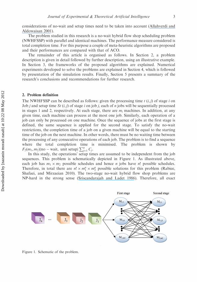
The NWHFSSP can be described as follows: given the processing time t (i, j) of stage i onJob j and setup time St (i, j) of stage i on job j, each of n jobs will be sequentially processedin stages 1 and 2, respectively. At each stage, there are mi machines. In addition, at anygiven time, each machine can process at the most one job. Similarly, each operation of ajob can only be processed on one machine. Once the sequence of jobs at the first stage isdefined, the same sequence is applied for the second stage. To satisfy the no-waitrestrictions, the completion time of a job on a given machine will be equal to the startingtime of the job on the next machine. In other words, there must be no waiting time betweenthe processing of any consecutive operations of each job. The problem is to find a sequencewhere the total completion time is minimised. The problem is shown byF2ðm1,m2Þjno� wait, unit setupj

Pnj¼1 Cj.

In this study, the operations’ setup times are assumed to be independent from the jobsequences. This problem is schematically depicted in Figure 1. As illustrated above,each job has m1 �m2 possible schedules and hence n jobs have n! possible schedules.Therefore, in total there are n!�mn

1 �mn2 possible solutions for this problem (Rabiee,

Shafaei, and Mirzaeian 2010). The two-stage no-wait hybrid flow shop problems areNP-hard in the strong sense (Sriscandarajah and Ladet 1986). Therefore, all exact

Figure 1. Schematic of the problem.

Journal of Experimental & Theoretical Artificial Intelligence 3

Dow

nloa

ded

by [

naza

nin

mor

adi n

asab

] at

10:

22 0

8 M

ay 2

012

algorithms for even a simple flow shop and simple parallel machines will most likelyhave running times that increase exponentially with the size of the problem. In this article,we propose two meta-heuristic algorithms for the problem described above. Theframeworks of the algorithms are explained in the next section.

3. Proposed algorithms

3.1. Adaptive imperialist competitive algorithm

Atashpaz-Gargari and Lucas (2007) illustrated the imperialist competitive algorithm(ICA). ICA has been widely applied for many non-polynomial hard optimisationproblems, such as flow shop and job shop scheduling. Shokrollahpour, Zandieh, andDorri (2011) applied this method for solving the two-stage assembly flow shop schedulingproblem with minimisation of weighted sum of makespan and mean completion time asthe objective. They calibrated the parameters of this algorithm using the Taguchi method.The results showed a satisfactory performance of the proposed algorithm.

ICA, similarly to other evolutionary algorithms, starts with an initial population inwhich every individual is named as a country. Countries are divided into two groups:imperialists and colonies. Some of the best countries (countries with the least costs) arechosen to be the imperialist countries and the rest, known as colonies, are divided amongthe imperialists based on their power. The power of each country is calculated based on theobjective function. A set of one imperialist and their colonies forms one empire. The totalpower of an empire is equal to the power of the imperialist country plus a percentageof mean power of its colonies. After forming initial empires, the competition starts; thecolonies in each empire starts moving toward their imperialist country, and the imperialistsattempt to achieve more colonies. Hence, during the competition, the weak imperialist willcollapse. At the end, just one imperialist will remain. The framework of the proposedadapted ICA (AICA) is described as follows.

3.1.1. Generating initial empires

Each solution in AICA is in a form of an array. Each array consists of variable values tobe optimised. In GA terminology, this array is called a ‘chromosome’, but here, the term‘country’ is used. In an N dimensional optimisation problem, a country is a 1�N array.This array is defined below:

country ¼ ½ p1, p2, p3, . . . , pN�, ð1Þ

where Pi is the variable to be optimised, each variable in a country denotes a socio-politicalcharacteristic of a country. From this point of view, the algorithm searches for the bestcountry, that is the country with the best combination of socio-political characteristicssuch as culture, language and economical policy (Atashpaz-Gargari and Lucas 2007).

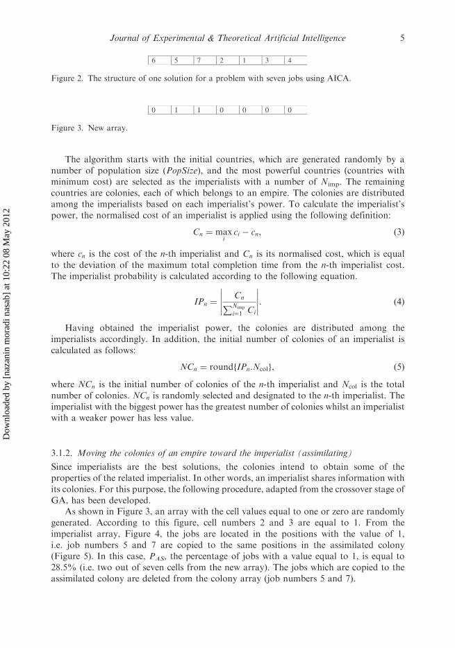
In AICA, each solution (country) is a 1 � N array of integer variables, where Nrepresents the number of jobs. The array of the country represents a sequence of jobs to beassigned to the earliest available machines in both stages. The structure of one solutionfor a problem with seven jobs is shown in Figure 2.

The cost of a country is calculated using a cost function f with the variablesðP1,P2, . . . ,PNÞ as follows:

ci ¼ f ðcountryiÞ ¼ f ð pi1, pi2, . . . , piNÞ: ð2Þ

4 N. Moradinasab et al.

Dow

nloa

ded

by [

naza

nin

mor

adi n

asab

] at

10:

22 0

8 M

ay 2

012

The algorithm starts with the initial countries, which are generated randomly by anumber of population size (PopSize), and the most powerful countries (countries withminimum cost) are selected as the imperialists with a number of Nimp. The remainingcountries are colonies, each of which belongs to an empire. The colonies are distributedamong the imperialists based on each imperialist’s power. To calculate the imperialist’spower, the normalised cost of an imperialist is applied using the following definition:

Cn ¼ maxi

ci � cn, ð3Þ

where cn is the cost of the n-th imperialist and Cn is its normalised cost, which is equalto the deviation of the maximum total completion time from the n-th imperialist cost.The imperialist probability is calculated according to the following equation.

IPn ¼Cn

PNimp

i¼1 Ci

�����

�����: ð4Þ

Having obtained the imperialist power, the colonies are distributed among theimperialists accordingly. In addition, the initial number of colonies of an imperialist iscalculated as follows:

NCn ¼ round IPn:Ncolf g, ð5Þ

where NCn is the initial number of colonies of the n-th imperialist and Ncol is the totalnumber of colonies. NCn is randomly selected and designated to the n-th imperialist. Theimperialist with the biggest power has the greatest number of colonies whilst an imperialistwith a weaker power has less value.

3.1.2. Moving the colonies of an empire toward the imperialist (assimilating)

Since imperialists are the best solutions, the colonies intend to obtain some of theproperties of the related imperialist. In other words, an imperialist shares information withits colonies. For this purpose, the following procedure, adapted from the crossover stage ofGA, has been developed.

As shown in Figure 3, an array with the cell values equal to one or zero are randomlygenerated. According to this figure, cell numbers 2 and 3 are equal to 1. From theimperialist array, Figure 4, the jobs are located in the positions with the value of 1,i.e. job numbers 5 and 7 are copied to the same positions in the assimilated colony(Figure 5). In this case, PAS, the percentage of jobs with a value equal to 1, is equal to28.5% (i.e. two out of seven cells from the new array). The jobs which are copied to theassimilated colony are deleted from the colony array (job numbers 5 and 7).

0 1 1 0 0 0 0

Figure 3. New array.

6 5 7 2 1 3 4

Figure 2. The structure of one solution for a problem with seven jobs using AICA.

Journal of Experimental & Theoretical Artificial Intelligence 5

Dow

nloa

ded

by [

naza

nin

mor

adi n

asab

] at

10:

22 0

8 M

ay 2

012

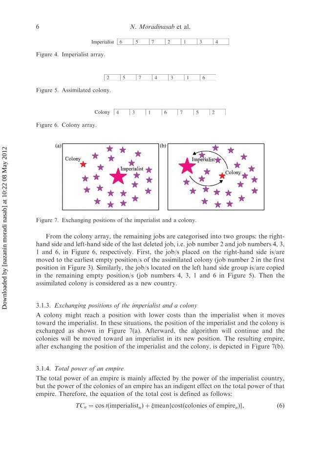
From the colony array, the remaining jobs are categorised into two groups: the right-hand side and left-hand side of the last deleted job, i.e. job number 2 and job numbers 4, 3,1 and 6, in Figure 6, respectively. First, the job/s placed on the right-hand side is/aremoved to the earliest empty position/s of the assimilated colony (job number 2 in the firstposition in Figure 3). Similarly, the job/s located on the left hand side group is/are copiedin the remaining empty position/s (job numbers 4, 3, 1 and 6 in Figure 5). Then theassimilated colony is considered as a new country.

3.1.3. Exchanging positions of the imperialist and a colony

A colony might reach a position with lower costs than the imperialist when it movestoward the imperialist. In these situations, the position of the imperialist and the colony isexchanged as shown in Figure 7(a). Afterward, the algorithm will continue and thecolonies will be moved toward an imperialist in its new position. The resulting empire,after exchanging the position of the imperialist and the colony, is depicted in Figure 7(b).

3.1.4. Total power of an empire

The total power of an empire is mainly affected by the power of the imperialist country,but the power of the colonies of an empire has an indigent effect on the total power of thatempire. Therefore, the equation of the total cost is defined as follows:

TCn ¼ cos tðimperialistnÞ þ �meanfcostðcolonies of empirenÞg, ð6Þ

Figure 7. Exchanging positions of the imperialist and a colony.

2 5 7 4 3 1 6

Figure 5. Assimilated colony.

4 3 1 6 7 5 2 Colony

Figure 6. Colony array.

6 5 7 2 1 3 4 Imperialist

Figure 4. Imperialist array.

6 N. Moradinasab et al.

Dow

nloa

ded

by [

naza

nin

mor

adi n

asab

] at

10:

22 0

8 M

ay 2

012

where TCn is the total cost of the n-th empire and xi (�) is a positive number considered tobe less than 1. The total power of the empire is determined by the imperialist, when thevalue of � is very small. The role of the colonies, which determines the total power of anempire, becomes more important as the value of � increases.

3.1.5. Imperialistic competition

All empires attempt to take possession of and control colonies of other empires. In theimperialistic competition, the power of weaker empires will gradually reduce and thepower of more powerful ones will rise. In other words, picking some (usually one) ofthe weakest colonies of the weakest empire and making a competition among all empiresto possess these colonies is the imperialistic competition. In this competition, the mostpowerful empires will most likely possess these colonies, but this is not definite. Thiscompetition is modelled by picking one of the weakest colonies from the weakest empire.In order to calculate the possession probability of each empire, first the normalised totalcost is calculated as follows:

NTCn ¼ max TCif g � TCn, ð7Þ

where NTCn is the normalised total cost of the n-th empire and TCn is the total cost of then-th empire. Having normalised the total cost, each empire’s probability is calculated asbelow:

EPn ¼NTCn

PNimp

i¼1 NTCi

�����

�����: ð8Þ

The roulette wheel method is used for assigning the mentioned colony to the empires.

3.1.6. Revolution

In each iteration, for every imperialist, two positions of the imperialist’s array are chosenand these positions are swapped and the new imperialist is replaced with the weakestimperialist colony. These processes are repeated by a percentage of jobs for eachimperialist, PIR. Furthermore, some of the colonies are selected and then two positions ofthe colony’s array are chosen and these positions are swapped. These processes arerepeated for a percentage of jobs for each colony, PCR. The replacement ratio is identifiedas the revolution rate, PR.

3.1.7. Eliminating the powerless empires

Powerless empires will collapse and their colonies will be distributed among other empiresin the imperialistic competition. In this article, when an empire loses all of its colonies,we consider it to be a collapsed empire.

3.1.8. Global war

One of the problems in the original ICA is the possibility of sticking in local optimalsolutions, which leads to a premature convergence. In this article, in order to solve thisproblem, a new concept called ‘global’ war has been developed. This is described as follows.

First, the value of two parameters, DGW and NGW, are determined. DGW and NGW areconsidered as the duration between two subsequent global wars and the total number ofglobal wars, respectively.

Journal of Experimental & Theoretical Artificial Intelligence 7

Dow

nloa

ded

by [

naza

nin

mor

adi n

asab

] at

10:

22 0

8 M

ay 2

012

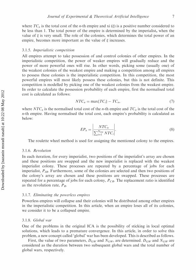
At the event of each global war, K countries, which are equal to the initial population,are randomly generated. This is considered as a new population.

The new and old populations are merged and sorted in ascending order in terms of thefitness function and the K best countries are selected accordingly. This is considered as anew population to be used for the next decade.

3.1.9. Stopping criteria

In this article, the algorithm stops when it reaches a situation with one empire or when acertain number of iterations (i.e. MaxDc) are repeated (Forouharfard and Zandieh 2010;Nazari-Shirkouhi, Eivazy, Ghodsi, Rezaie, and Atashpaz-Gargari 2010). Figure 8 givesAICA in pseudo code. Another can be used to stop the algorithm, when its best solution indifferent decades cannot be improved for some consecutive decades (Nazari-Shirkouhiet al. 2010).

3.2. Proposed genetic algorithm

Goldberg (1989) was the one who first described the usual form of the genetic algorithm(GA). GA is based on the mechanism of natural selection and has a wide application insolving scheduling and other operations research problems (Onwubolu and Mutingi 1999;Ponnambalam, Ramkumar, and Jawahar 2001; Mansouri, Moattar-Husseini, and Zegordi2003; Hao et al. 2005). The framework of GA is described in the next subsections.

3.2.1. Chromosome representation

A chromosome in a GA is trail of genes, the chromosome is considered as a possiblesolution, which is a 1�N array of integer variables, whereN represents the number of jobs.

Figure 8. AICA in pseudo code.

8 N. Moradinasab et al.

Dow

nloa

ded

by [

naza

nin

mor

adi n

asab

] at

10:

22 0

8 M

ay 2

012

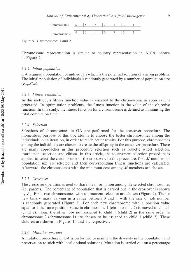
Chromosome representation is similar to country representation in AICA, shownin Figure 2.

3.2.2. Initial population

GA requires a population of individuals which is the potential solution of a given problem.The initial population of individuals is randomly generated by a number of population size(PopSize).

3.2.3. Fitness evaluation

In this method, a fitness function value is assigned to the chromosome as soon as it isgenerated. In optimisation problems, the fitness function is the value of the objectivefunction. In this study, the fitness function for a chromosome is defined as minimising thetotal completion time.

3.2.4. Selection

Selections of chromosomes in GA are performed for the crossover procedure. Themomentous purpose of this operator is to choose the better chromosomes among theindividuals in an iteration, in order to reach better results. For this purpose, chromosomesamong the individuals are chosen to create the offspring in the crossover procedure. Thereare many approaches in this procedure selection such as roulette wheel selection,tournament selection and elitism. In this article, the tournament selection procedure isapplied to select the chromosome of the crossover. In this procedure, first M numbers ofpopulation size are selected and then corresponding fitness functions are calculated.Afterward, the chromosomes with the minimum cost among M members are chosen.

3.2.5. Crossover

The crossover operation is used to share the information among the selected chromosomes(i.e. parents). The percentage of population that is carried out in the crossover is shownby PC. First, two chromosomes with tournament selection are chosen (Figure 9). Then anew binary mask varying in a range between 0 and 1 with the size of job numberis randomly generated (Figure 3). For each new chromosome with a position valueequal to 1 the same position value in chromosome 1 (chromosome 2) is moved to child 1(child 2). Then, the other jobs not assigned to child 1 (child 2) in the same order inchromosome 2 (chromosome 1) are chosen to be assigned to child 1 (child 2). Thesechildren are shown in Figures 10 and 11, respectively.

3.2.6. Mutation operator

A mutation procedure in GA is performed to maintain the diversity in the population andpreservation to stick with local optimal solutions. Mutation is carried out on a percentage

6 5 7 2 1 3 4

4 3 1 6 7 5 2

Chromosome 1

Chromosome 2

Figure 9. Chromosomes 1 and 2.

Journal of Experimental & Theoretical Artificial Intelligence 9

Dow

nloa

ded

by [

naza

nin

mor

adi n

asab

] at

10:

22 0

8 M

ay 2

012

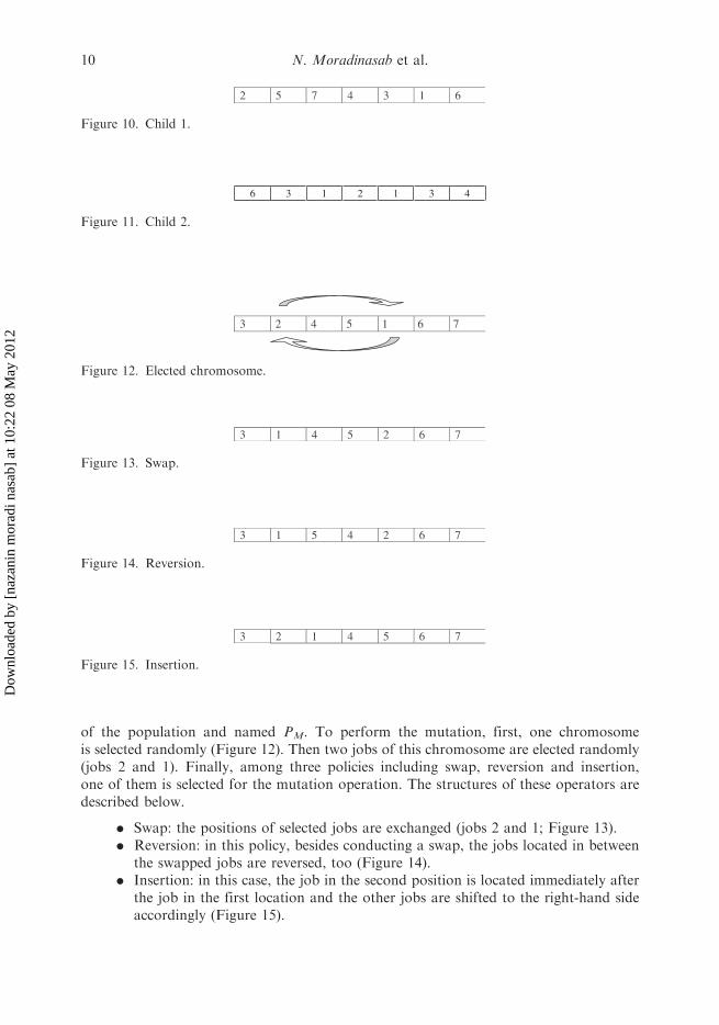
of the population and named PM. To perform the mutation, first, one chromosomeis selected randomly (Figure 12). Then two jobs of this chromosome are elected randomly(jobs 2 and 1). Finally, among three policies including swap, reversion and insertion,one of them is selected for the mutation operation. The structures of these operators aredescribed below.

. Swap: the positions of selected jobs are exchanged (jobs 2 and 1; Figure 13).

. Reversion: in this policy, besides conducting a swap, the jobs located in betweenthe swapped jobs are reversed, too (Figure 14).

. Insertion: in this case, the job in the second position is located immediately afterthe job in the first location and the other jobs are shifted to the right-hand sideaccordingly (Figure 15).

3 2 4 5 1 6 7

Figure 12. Elected chromosome.

6 3 1 2 1 3 4

Figure 11. Child 2.

2 5 7 4 3 1 6

Figure 10. Child 1.

3 2 1 4 5 6 7

Figure 15. Insertion.

3 1 5 4 2 6 7

Figure 14. Reversion.

3 1 4 5 2 6 7

Figure 13. Swap.

10 N. Moradinasab et al.

Dow

nloa

ded

by [

naza

nin

mor

adi n

asab

] at

10:

22 0

8 M

ay 2

012

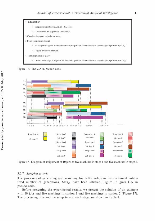
3.2.7. Stopping criteria

The processes of generating and searching for better solutions are continued until a

fixed number of generations, MaxIt, have been satisfied. Figure 16 gives GA in

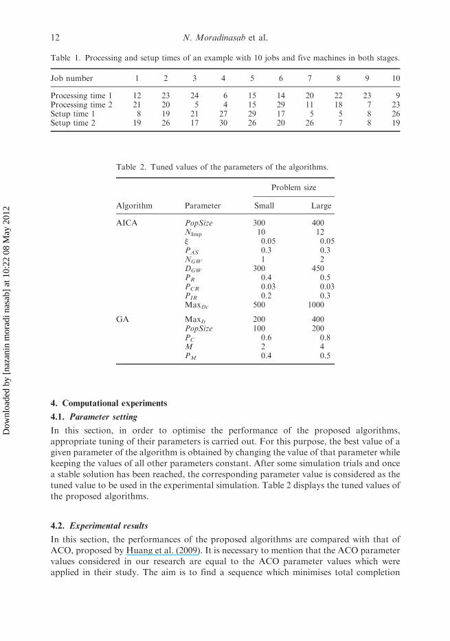
pseudo code.Before presenting the experimental results, we present the solution of an example

with 10 jobs and five machines in station 1 and five machines in station 2 (Figure 17).

The processing time and the setup time in each stage are shown in Table 1.

Figure 17. Diagram of assignment of 10 jobs to five machines in stage 1 and five machines in stage 2.

1-Initialization

1-1-set parameters (PopSize, M, PC , PM, MaxIt)

1-2- Generate initial population (Randomly).

2-Calculate fitness of each chromosome.

3-Form population 2 (pop2)

3-1-Select percentage of PopSize for crossover operation with tournament selection (with probability of PC ).

3-2- Apply crossover operator.

4- Form population 3 (pop3)

4-1- Select percentage of PopSize for mutation operation with tournament selection (with probability of PM).

Figure 16. The GA in pseudo code.

Journal of Experimental & Theoretical Artificial Intelligence 11

Dow

nloa

ded

by [

naza

nin

mor

adi n

asab

] at

10:

22 0

8 M

ay 2

012

4. Computational experiments

4.1. Parameter setting

In this section, in order to optimise the performance of the proposed algorithms,appropriate tuning of their parameters is carried out. For this purpose, the best value of agiven parameter of the algorithm is obtained by changing the value of that parameter whilekeeping the values of all other parameters constant. After some simulation trials and oncea stable solution has been reached, the corresponding parameter value is considered as thetuned value to be used in the experimental simulation. Table 2 displays the tuned values ofthe proposed algorithms.

4.2. Experimental results

In this section, the performances of the proposed algorithms are compared with that ofACO, proposed by Huang et al. (2009). It is necessary to mention that the ACO parametervalues considered in our research are equal to the ACO parameter values which wereapplied in their study. The aim is to find a sequence which minimises total completion

Table 2. Tuned values of the parameters of the algorithms.

Problem size

Algorithm Parameter Small Large

AICA PopSize 300 400NImp 10 12� 0.05 0.05PAS 0.3 0.3NGW 1 2DGW 300 450PR 0.4 0.5PCR 0.03 0.03PIR 0.2 0.3MaxDc 500 1000

GA MaxIt 200 400PopSize 100 200PC 0.6 0.8M 2 4PM 0.4 0.5

Table 1. Processing and setup times of an example with 10 jobs and five machines in both stages.

Job number 1 2 3 4 5 6 7 8 9 10

Processing time 1 12 23 24 6 15 14 20 22 23 9Processing time 2 21 20 5 4 15 29 11 18 7 23Setup time 1 8 19 21 27 29 17 5 5 8 26Setup time 2 19 26 17 30 26 20 26 7 8 19

12 N. Moradinasab et al.

Dow

nloa

ded

by [

naza

nin

mor

adi n

asab

] at

10:

22 0

8 M

ay 2

012

time. All algorithms studied were coded using MATLAB 2009b and run on a personal

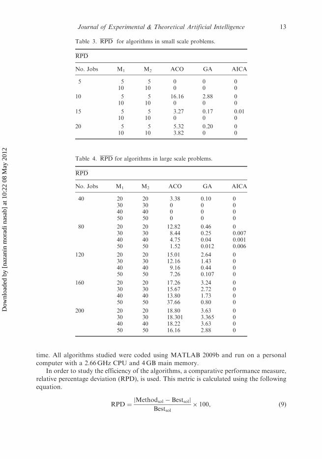
computer with a 2.66GHz CPU and 4GB main memory.In order to study the efficiency of the algorithms, a comparative performance measure,

relative percentage deviation (RPD), is used. This metric is calculated using the following

equation.

RPD ¼Methodsol � Bestsolj j

Bestsol� 100, ð9Þ

Table 4. RPD for algorithms in large scale problems.

RPD

No. Jobs M1 M2 ACO GA AICA

40 20 20 3.38 0.10 030 30 0 0 040 40 0 0 050 50 0 0 0

80 20 20 12.82 0.46 030 30 8.44 0.25 0.00740 40 4.75 0.04 0.00150 50 1.52 0.012 0.006

120 20 20 15.01 2.64 030 30 12.16 1.43 040 40 9.16 0.44 050 50 7.26 0.107 0

160 20 20 17.26 3.24 030 30 15.67 2.72 040 40 13.80 1.73 050 50 37.66 0.80 0

200 20 20 18.80 3.63 030 30 18.301 3.365 040 40 18.22 3.63 050 50 16.16 2.88 0

Table 3. RPD for algorithms in small scale problems.

RPD

No. Jobs M1 M2 ACO GA AICA

5 5 5 0 0 010 10 0 0 0

10 5 5 16.16 2.88 010 10 0 0 0

15 5 5 3.27 0.17 0.0110 10 0 0 0

20 5 5 5.32 0.20 010 10 3.82 0 0

Journal of Experimental & Theoretical Artificial Intelligence 13

Dow

nloa

ded

by [

naza

nin

mor

adi n

asab

] at

10:

22 0

8 M

ay 2

012

Table

5.Detailed

simulationresultsforsm

all-sizeproblems.

No.

jobs

M1

M2

ACO

GA

AIC

A

Best_Sol

Worst_Sol

Stdev_Sol

Mean_Sol

Best_Sol

Worst_Sol

Stdev_Sol

Mean_Sol

Best_Sol

Worst_Sol

Stdev_Sol

Mean_Sol

55

5240

240

0240

240

240

0240

240

240

0240

10

10

240

240

0240

240

240

0240

240

240

0240

10

55

622

630

2.780

625.833

621

621

0621

621

621

0621

10

10

484

484

0484

484

484

0484

484

484

0484

15

55

1174

1184

3.892817

1181.467

1144

1147

0.844863

1146.1

1144

1146

0.610257

1144.2

10

10

855

855

0855

855

855

0855

855

855

0855

20

55

1741

1768

12.94551

1750

1664

1666

0.691492

1664.93

1661

1664

1.220514

1661.6

10

10

1150

1166

7.636

1157.633

1115

1115

01115

1115

1115

01115

14 N. Moradinasab et al.

Dow

nloa

ded

by [

naza

nin

mor

adi n

asab

] at

10:

22 0

8 M

ay 2

012

Table

6.Detailed

simulationresultsforlarge-size

problems.

ACO

GA

AIC

A

No.

joubs

M1

M2

Best_Sol

Worst_Sol

Stdev_Sol

Mean_Sol

Best_Sol

Worst_Sol

Stdev_Sol

Mean_Sol

Best_Sol

Worst_Sol

Stdev_Sol

Mean_Sol

40

20

20

2434

2457

9.50

2448.16

2368

2372

1.65

2370.4

2368

2368

02368

30

30

2071

2071

02071

2071

2071

02071

2071

2071

02071

40

40

1886

1886

01886

1886

1886

01886

1886

1886

01886

50

50

1886

1886

01886

1886

1886

01886

1886

1886

01886

80

20

20

7236

7399

50.49

7346.03

6539

6544

1.79

6540.76

6505

6519

5.87

6511.06

30

30

5641

5661

8.92

5649.66

5220

5225

2.30

5222.73

5205

5224

7.68

5210.27

40

40

4706

4875

73.36

4784.73

4569

4570

0.51

4569.53

4567

4571

1.073

4567.77

50

50

4329

4344

5.30

4333.27

4268

4269

0.5

4268.6

4268

4269

0.48

4268.34

120

20

20

14995

15071

35.15

15032.73

13412

13425

3.451

13415.57

13062

13078

5.26

13070.17

30

30

11012

11075

31.76

11047.7

9930

10029

40.70

9990.73

9848

9854

2.39

9850.17

40

40

9043

9108

27.88

9070.86

8338

8358

8.76

8346.17

8305

8318

4.20

8309.24

50

50

7925

7969

20.03

7948.56

7416

7420

1.53

7418.067

7408

7414

2.15

7410.1

160

20

20

27768

27914

58.49

27835.67

24419

24709

125.05

24505.97

23705

23809

37.55

23737.1

30

30

20014

20077

28.01

20048.83

17725

17870

67.10

17805.13

17323

17349

7.82

17333.07

40

40

16130

16230

49.83

16190

14451

14494

16.84

14473.77

14218

14494

6.15

14226.47

50

50

13886

13944

24.25

13909.73

12516

12538

8.86

12527.8

12426

12432

2.22

12428.03

200

20

20

41382

41646

111.7134

41467.1

36082

36289

92.26106

36171.03

34876

34930

18.47151

34903.9

30

30

29271

29615

112.7999

29379.63

25560

25753

80.4386

25670.33

24824

24848

10.65

24834.43

40

40

23473

23762

94.36647

23604.07

20638

20721

36.15001

20692.07

19953

20006

15.21

19966.77

50

50

19794

19930

55.67526

19841.3

17544

17586

15.25

17572.83

17057

17113

21.38

17080.47

Journal of Experimental & Theoretical Artificial Intelligence 15

Dow

nloa

ded

by [

naza

nin

mor

adi n

asab

] at

10:

22 0

8 M

ay 2

012

where Methodsol is the value of a method and Bestsol is the best value obtained among

the algorithms. Also, RPD is defined according to the following equation:

RPD ¼

P30i¼1 RPD

30: ð10Þ

The performance of the algorithms was testified by solving 28 different problems in

two scales (eight problems in small scale and 20 problems in large scale). These problems

AICAGAACO

2.0

1.5

1.0

0.5

0.0

Algorithms

RPD

Interval Plot of ACO, GA, AICA

95% CI for the Mean

Figure 18. Confidence interval 95% for RPD of algorithms for small scale.

AICAGAACO

12

10

8

6

4

2

0

Algorithms

RPD

Interval Plot of ACO, GA, AICA

95% CI for the Mean

Figure 19. Confidence interval 95% for RPD of algorithms for large scale.

16 N. Moradinasab et al.

Dow

nloa

ded

by [

naza

nin

mor

adi n

asab

] at

10:

22 0

8 M

ay 2

012

are those used by Huang et al. (2009). Tables 3 and 4 show the comparative results in termsof RPD (for total completion time) of the proposed algorithms and ACO for small andlarge scale, respectively. The results presented in Table 3 show that in small-scale problemsthe AICA algorithm outperformed the other algorithms. This is followed by GA, which isalso superior to ACO. In addition, the results presented in Table 4 indicate that, similarlyto the small scale problems, for large scale problems, AICA and GA are superior to ACOwhile AICA obtained the best performance.

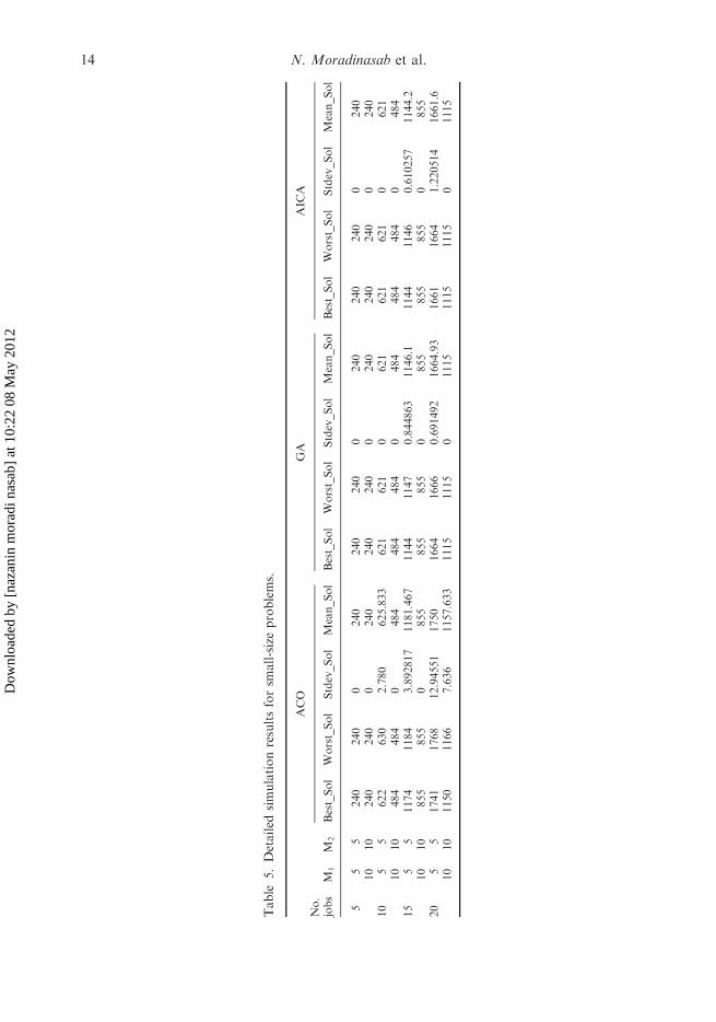
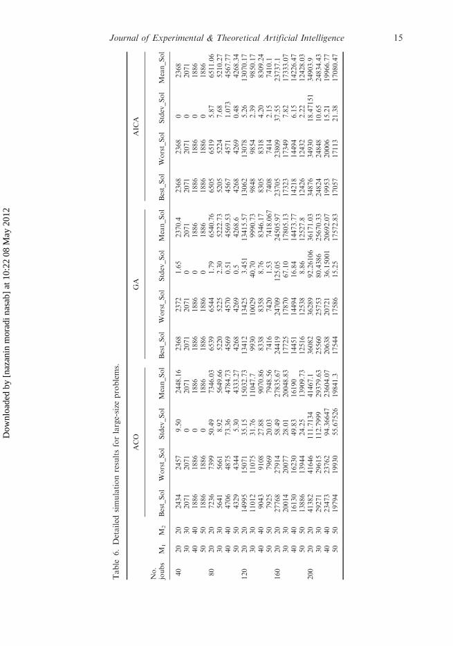
Tables 5 and 6 show the detailed results in terms of best solution, worst solution, meanof solutions and standard deviation of the solutions for small- and large-scale problems.The results reveal that AICA has a higher efficiency than that of GA and ACO.

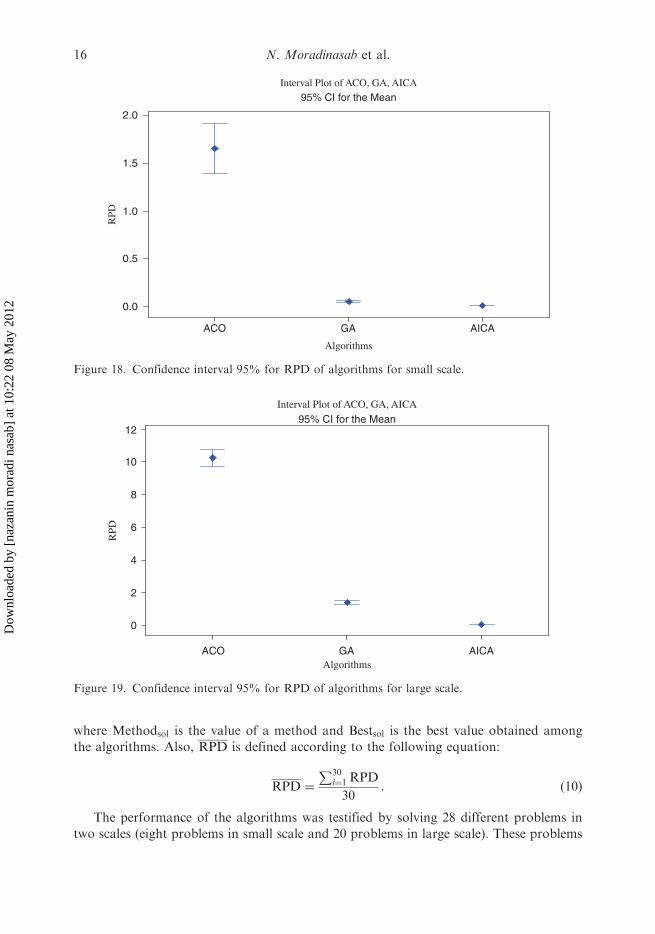
In order to evaluate the significance of the results presented earlier, a statisticalevaluation in terms of RPD with 95% confidence interval was conducted. The results arepresented in Figures 18 and 19. The results indicate that for both scale problems, AICAstatistically outperforms the other algorithms followed by GA, which outperforms ACO.Therefore, it can be concluded that the proposed algorithms in both scales have a superiorperformance to that of ACO.

Figure 20 shows the performance of the algorithms with respect to the number of jobs.This shows that the performance of ACO and GA deteriorate as the number of jobsincreases. However, AICA has constant superiority for all of the problems.

5. Conclusion

This paper focuses on solving the problem of a no-wait two-stage hybrid flow shopwith unit setup times. For this purpose, two efficient meta-heuristic algorithms, AICA andGA, are proposed. The performance measure considered is the minimum total completiontime. In order to assess the performance of the proposed algorithms, comparativeanalogies among the algorithms are applied in terms of relative percentage deviation.

Figure 20. Means plot and Tukey intervals 95% for the interaction between the type of algorithmand number of jobs.

Journal of Experimental & Theoretical Artificial Intelligence 17

Dow

nloa

ded

by [

naza

nin

mor

adi n

asab

] at

10:

22 0

8 M

ay 2

012

The results of the simulation study indicate that AICA significantly outperforms GA andACO. Furthermore, GA obtained a superior performance than ACO. The results also

show that the performance of ACO and GA deteriorate as the number of jobs increases.However, AICA obtained constantly superior performance in solving the problemsin different sizes. As a further study, it is proposed to consider job release time and reworktime in the problem studied. In addition, it is worthwhile studying the performance of theproposed algorithm in terms of other performance measures such as mean flow time and

mean tardiness.

Acknowledgements

The authors are grateful for the valuable comments and suggestions from the respected reviewers.We believe that their valuable comments and suggestions have enhanced the strength andsignificance of this article.

References

Allahverdi, A., and Aldowaisan, T. (2001), ‘Minimizing Total Completion Time in a No-wait

Flowshop with Sequence-dependent Additive Changeover Times’, Journal of the Operational

Research Society, 52, 449–462.Atashpaz-Gargari, and Lucas, E.C. (2007), ‘Imperialist Competitive Algorithm: An Algorithm

for Optimization Inspired by Imperialist Competitive’, in IEEE Congress on Evolutionary

computation, Singapore, pp. 4661–4666.Bonney, M.C., and Gundry, S.W. (1976), ‘Solutions to the Constrained Flow Shop Sequencing

Problem’, Operational Research Quarterly, 24, 869–883.

Forouharfard, S., and Zandieh, M. (2010), ‘An Imperialist Competitive Algorithm to Schedule of

Receiving and Shipping Trucks in Cross-docking Systems’, International Journal of Advanced

Manufacturing Technology, 51, 1179–1193.Gilmore, P.C., and Gomory, E. (1964), ‘Sequencing a One State-variable Machine: A Solvable Case

of the Traveling Salesman Problem’, Operations Research, 12, 655–679.Goldberg, D.E. (1989), Genetic Algorithms in Search, Optimization and Machine Learning, Reading,

MA: Addison-Wesley.Hao, G., Gong, D., Shi, Y., and Wang, L. (2005), ‘Interactive Genetic Algorithm Based on

Landscape of Satisfaction and Taboos’, Journal of China University of Mining & Technology,

34(2), 204–208.Haouari, M., Hidri, L., and Gharbi, A. (2006), ‘Optimal Scheduling of a Two-stage Hybrid Flow

Shop’, Mathematical Methods Operations Research, 64, 107–124.

Huang, R.H., Yang, C.L., and Huang, Y.C. (2009), ‘No-wait Two-stage Multiprocessor Flow

Shop Scheduling with Unit Setup’, Internationl Journal of Advanced Manufacturing

Technology, 44, 921–927.Jayamohan, M.S., and Rajendran, C. (2000), ‘A Comparative Analysis of Two Different

Approaches to Scheduling in Flexible Flow Shops’, Production Planning & Control, 11,

572–580.Jolai, F., Sheikh, S., Rabbani, M., and Karimi, B. (2009), ‘A Genetic Algorithm for Solving No-wait

Flexible Flow Lines with Due Window and Job Rejection’, The International Journal of

Advanced Manufacturing Technology, 42, 523–532.

King, J.R., and Spachis, A.S. (1980), ‘Heuristics for Flows Hop Scheduling’, International Journal of

Production Research, 18, 343–357.

18 N. Moradinasab et al.

Dow

nloa

ded

by [

naza

nin

mor

adi n

asab

] at

10:

22 0

8 M

ay 2

012

Mansouri, S.A., Moattar-Husseini, S.M., and Zegordi, S.H. (2003), ‘A Genetic Algorithm forMultiple Objective Dealing with Exceptional Elements in Cellular Manufacturing’, ProductionPlanning & Control, 14, 437–446.

Nazari-Shirkouhi, S., Eivazy, H., Ghodsi, R., Rezaie, K., and Atashpaz-Gargari, E. (2010), ‘Solving

the Integrated Product Mix-outsourcing Problem Using the Imperialist CompetitiveAlgorithm’, Expert Systems with Applications, 37, 7615–7626.

Onwubolu, G.C., and Mutingi, M. (1999), ‘Genetic Algorithm for Minimizing Tardiness in

Flow-shop Scheduling’, Production Planning & Control, 10, 462–471.Ponnambalam, S.G., Ramkumar, V., and Jawahar, N. (2001), ‘A Multiobjective Genetic Algorithm

for Job Shop Scheduling’, Production Planning & Control, 12, 764–774.

Rabiee, M., Shafaei, R., and Mirzaeian, M. (2010), ‘Generating an Efficient Schedule in a No-waitTwo Stage Flexible Flow Shops with Maximizing Utilization’, in The InternationalConference on Industrial Engineering and Business Management (ICIEBM) Jakarta,

Indonesia, pp. 555–561.Rajendran, C. (1994), ‘A No-wait Flow Shop Scheduling Heuristic for Minimizing Makespan’,

Journal of the Operational Research Society, 45, 472–478.Rajendran, C., and Chaudhuri, D. (1990), ‘Heuristic Algorithms for Continuous Flow Shop

Problem’, Naval Research Logistics, 37, 695–705.Reddi, S.S., and Ramamoorthy, C.V. (1972), ‘On the Flow Shop Sequencing Problem with No-wait

in Process’, Operational Research Quarterly, 23, 323–331.

Rock, H. (1984), ‘The Three-machine No-wait Flow Shop Problem is NP-complete’, Journal ofAssociate Computer Machinery, 31, 336–345.

Ruiz, R., and Allahverdi, A. (2007), ‘No-wait Flowshop with Separate Setup Times to Minimize

Maximum Lateness’, The International Journal of Advanced Manufacturing Technology, 35,551–565.

Santos, D.L., Hunsucker, J.L., and Deal, D.E. (2001), ‘On Makespan Improvement in Flow Shopswith Multiple Processors’, Production Planning & Control, 12, 283–295.

Shafaei, R., Rabiee, M., and Mirzaeyan, M. (2011), ‘An Adaptive Neuro Fuzzy Inference System forMakespan Estimation in Multiprocessor No-wait Two Stage Flow Shop’, InternationalJournal of Computer Integrated Manufacturing, 24(10), 888–899.

Shokrollahpour, E., Zandieh, M., and Dorri, B. (2011), ‘A Novel Imperialist Competitive Algorithmfor Bi-criteria Scheduling of the Assembly Flowshop Problem’, International Journal ofProduction Research, 49, 3087–3103.

Sriscandarajah, C., and Ladet, P. (1986), ‘Some No-wait Shops Scheduling Problems: ComplexityAspects’, European Journal of Operational Research, 24, 424–445.

Van Deman, J.M., and Baker, K.R. (1974), ‘Minimizing Flowtime in the Flow Shop with no

Intermediate Queues’, IIE Transactions, 6, 28–34.Wang, Z., Xing, W., and Bai, F. (2005), ‘No-wait Flexible Flow Shop Scheduling with No-idle

Machines’, Operations Research Letters, 33, 609–614.Wismer, D.A. (1972), ‘Solution of the Flow Shop Sequencing Problem with no Intermediate

Queues’, Operations Research, 20, 689–697.

Journal of Experimental & Theoretical Artificial Intelligence 19

Dow

nloa

ded

by [

naza

nin

mor

adi n

asab

] at

10:

22 0

8 M

ay 2

012