High-Performance Algorithms for Compile-Time Scheduling of ...

High-Performance Algorithms for Compile-TimeScheduling of Parallel Processors

By

Yu-Kwong KWOK

A Thesis Presented to

The Hong Kong University of Science and Technology

in Partial Fulfillment

of the Requirements for

the Degree of Doctor of Philosophy

in Computer Science

Hong Kong, May 1997

Copyright by Yu-Kwong KWOK 1997

- i -

Authorization

I hereby declare that I am the sole author of the thesis.

I authorize the Hong Kong University of Science and Technology to lend this thesis to

other institutions or individuals for the purpose of scholarly research.

I further authorize the Hong Kong University of Science and Technology to reproduce the

thesis by photocopying or by other means, in total or in part, at the request of other

institutions or individuals for the purpose of scholarly research.

- ii -


By

Yu-Kwong KWOK

APPROVED:

Dr. Ishfaq AHMAD, SUPERVISOR

Prof. Roland T. CHIN, HEAD OF DEPARTMENT

Department of Computer Science, HKUST

May 1997

- iii -

Acknowledgments

The completion of this thesis would not have been possible without the help and

encouragement of my advisor, colleagues, and many professional acquaintances. I would like

to thank all the people who have helped me in one way or another to complete my research

work. In particular, I would like to thank my advisor, Dr. Ishfaq Ahmad, for introducing the

field of parallel and distributed computing to me, and for his continual support on both

academic and personal problems. Indeed, his guidance and advice have had a major positive

impact on my development as a scientific researcher and as an individual. I am most grateful

to my wife, Fyon, for her love and support on my studies that kept me going on whenever I

was tired and frustrated. Without her encouragement, it would have been difficult to finish

my doctoral studies.

I would also like to thank the other members of the thesis examination committee:

Professor Ming L. Liou, Professor Michael Palis1, Dr. Ting-Chuen Pong, and Professor Derick

Wood, for their helpful reviews and comments on the thesis. In particular, I am very grateful

to Professor Derick Wood for his insightful advice and helpful technical suggestions. Thanks

are also due to Dr. Dik-Lun Lee for his valuable comments on my research work. I would also

like to thank our head of department, Professor Roland Chin, for his kindness and

encouragements. I am also very grateful to our English tutor, Miss Elut Kwok, for her

invaluable help in improving the presentation of the thesis. I would also like to take this

opportunity to thank my other teachers including Dr. Manhoy Choi, Dr. Mordecai Golin, Dr.

Jun Gu, Dr. Jogesh Muppala, Dr. Tin-Fook Ngai, and Dr. Dit-Yan Yeung.

I would like to acknowledge the Hong Kong Research Grants Council for supporting this

work (under contract number HKUST 734/96E). Last but not the least, I would like to thank

the Computer Science Department for its generosity in providing a nice, convenient, and

professional environment for its graduate students.

1. Professor at the Department of Computer Science, Rutgers University, Camden, NJ, USA.

- iv -

Dedication

To Fyon and our parents

- v -

Table of Contents

Authorization Page............................................................................................................................... i

Signature Page...................................................................................................................................... ii

Acknowledgments.............................................................................................................................. iii

Dedication............................................................................................................................................ iv

Table of Contents.................................................................................................................................. v

List of Figures ...................................................................................................................................... ix

List of Tables ....................................................................................................................................... xv

List of Symbols ................................................................................................................................xviii

Abstract .............................................................................................................................................. xix

Chapter 1 Introduction . . . . . . . . . . . . . . . . . . . . . . . . . . . . . . . . . . . . . . . . . .1

1.1 Overview.................................................................................................................................. 1

1.2 Parallel Architectures and The Scheduling Problem......................................................... 3

1.3 Research Objectives ................................................................................................................ 5

1.4 Contributions........................................................................................................................... 6

1.5 Organization of the Thesis .................................................................................................... 7

Chapter 2 Background and Literature Survey . . . . . . . . . . . . . . . . . . . . . .9

2.1 Introduction............................................................................................................................. 9

2.2 Problem Statement and The Models Used........................................................................ 13

2.2.1 The DAG Model .......................................................................................................... 14

2.2.2 DAG Generation ......................................................................................................... 14

2.2.3 Variations of the DAG Model ................................................................................... 15

2.2.4 The Multiprocessor Model ........................................................................................ 16

2.3 NP-Completeness of the Scheduling Problem ................................................................. 16

2.4 Basic Techniques in DAG Scheduling ............................................................................... 18

2.5 A Taxonomy of DAG Scheduling Algorithms ................................................................. 21

2.6 Survey of DAG Scheduling Algorithms............................................................................ 23

2.6.1 Scheduling DAGs with Restricted Structures......................................................... 23

2.6.1.1 Hu’s Algorithm for Tree-Structured DAGs ........................................................ 24

- vi -

2.6.1.2 Coffman and Graham’s Algorithm for Two-Processor Scheduling ................ 25

2.6.1.3 Scheduling Interval-Ordered DAGs .................................................................... 27

2.6.2 Scheduling Arbitrary DAGs without Communication ......................................... 27

2.6.2.1 Level-based Heuristics ........................................................................................... 27

2.6.2.2 A Branch-and-Bound Approach........................................................................... 28

2.6.2.3 Analytical Performance Bounds for Scheduling without Communication ... 29

2.6.3 UNC Scheduling ......................................................................................................... 31

2.6.3.1 Scheduling of Primitive Graph Structures .......................................................... 31

2.6.3.2 The EZ Algorithm ................................................................................................... 32

2.6.3.3 The LC Algorithm................................................................................................... 33

2.6.3.4 The DSC Algorithm ................................................................................................ 34

2.6.3.5 The MD Algorithm ................................................................................................. 36

2.6.3.6 The DCP Algorithm................................................................................................ 37

2.6.3.7 Other UNC Approaches......................................................................................... 39

2.6.3.8 Theoretical Analysis for UNC Scheduling .......................................................... 40

2.6.4 BNP Scheduling .......................................................................................................... 40

2.6.4.1 The HLFET Algorithm ........................................................................................... 40

2.6.4.2 The ISH Algorithm ................................................................................................. 42

2.6.4.3 The MCP Algorithm ............................................................................................... 42

2.6.4.4 The ETF Algorithm ................................................................................................. 45

2.6.4.5 The DLS Algorithm................................................................................................. 46

2.6.4.6 The LAST Algorithm .............................................................................................. 47

2.6.4.7 Other BNP Approaches.......................................................................................... 49

2.6.4.8 Analytical Performance Bounds of BNP Scheduling......................................... 51

2.6.5 TDB Scheduling........................................................................................................... 51

2.6.5.1 The PY Algorithm ................................................................................................... 52

2.6.5.2 The LWB Algorithm ............................................................................................... 53

2.6.5.3 The DSH Algorithm................................................................................................ 54

2.6.5.4 The BTDH Algorithm............................................................................................. 55

2.6.5.5 The LCTD Algorithm ............................................................................................. 56

2.6.5.6 The CPFD Algorithm.............................................................................................. 58

2.6.5.7 Other TDB Approaches.......................................................................................... 60

2.6.6 APN Scheduling.......................................................................................................... 62

2.6.6.1 The Message Routing Issue ................................................................................... 62

2.6.6.2 The MH Algorithm ................................................................................................. 63

2.6.6.3 The DLS Algorithm................................................................................................. 64

- vii -

2.6.6.4 The BU Algorithm................................................................................................... 65

2.6.6.5 The BSA Algorithm................................................................................................. 67

2.6.6.6 Other APN Approaches ......................................................................................... 69

2.6.7 Scheduling in Heterogeneous Environments ......................................................... 70

2.6.8 Mapping Clusters to Processors ............................................................................... 71

2.7 Summary and Concluding Remarks.................................................................................. 73

Chapter 3 A Low Complexity Scheduling Algorithm . . . . . . . . . . . . . . .75

3.1 Introduction........................................................................................................................... 75

3.2 Scheduling Using Neighborhood Search .......................................................................... 76

3.3 The Proposed Algorithms ................................................................................................... 78

3.3.1 A Solution Neighborhood Formulation .................................................................. 78

3.3.2 The Sequential FAST Algorithm............................................................................... 79

3.3.3 The PFAST Algorithm................................................................................................ 82

3.4 An Example ........................................................................................................................... 83

3.5 Performance Results............................................................................................................. 84

3.5.1 Number of Search Steps............................................................................................. 86

3.5.2 CASCH ......................................................................................................................... 86

3.5.3 Applications................................................................................................................. 88

3.5.4 Results of the PFAST Algorithm Compared against Optimal Solutions............ 89

3.5.5 Large DAGs ................................................................................................................. 94

3.6 Summary and Concluding Remarks.................................................................................. 95

Chapter 4 Scheduling using Parallel Genetic Search . . . . . . . . . . . . . . . .98

4.1 Introduction........................................................................................................................... 98

4.2 Overview of Genetic Search Techniques......................................................................... 100

4.2.1 Standard Genetic Algorithms ................................................................................. 100

4.2.2 Genetic Search Operators ........................................................................................ 101

4.2.3 Control Parameters................................................................................................... 103

4.2.4 Parallel Genetic Algorithms .................................................................................... 103

4.3 The Proposed Parallel Genetic Algorithm for Scheduling ........................................... 104

4.3.1 A Scrutiny of List Scheduling ................................................................................. 104

4.3.2 A Genetic Formulation of the Scheduling Problem............................................. 106

4.3.3 Genetic Operators ..................................................................................................... 108

4.3.4 Control Parameters................................................................................................... 112

- viii -

4.3.5 Parallelization............................................................................................................ 113

4.4 Performance Results........................................................................................................... 114

4.4.1 Comparison against Optimal Solutions................................................................. 115

4.4.2 Comparison with the PFAST Algorithm............................................................... 119

4.4.3 Results on Regular Graphs ...................................................................................... 120

4.5 Related Work....................................................................................................................... 125

4.6 Summary and Concluding Remarks................................................................................ 127

Chapter 5 A Parallel Algorithm for APN Scheduling . . . . . . . . . . . . . .128

5.1 Introduction......................................................................................................................... 128

5.2 The Proposed Algorithm ................................................................................................... 128

5.2.1 Scheduling Serially ................................................................................................... 129

5.2.2 Scheduling in Parallel............................................................................................... 133

5.3 An Example ......................................................................................................................... 137

5.4 Performance Results........................................................................................................... 143

5.5 Summary and Concluding Remarks................................................................................ 154

Chapter 6 Conclusions and Future Research . . . . . . . . . . . . . . . . . . . . .156

6.1 Summary.............................................................................................................................. 156

6.1.1 A Low Time-Complexity Algorithm...................................................................... 158

6.1.2 Scheduling using Parallel Genetic Search ............................................................. 158

6.1.3 A Parallel Algorithm for Scheduling under Realistic Environments................ 159

6.2 Future Research Directions ............................................................................................... 160

References ......................................................................................................................................... 162

Vita ..................................................................................................................................................... 176

- ix -

List of Figures

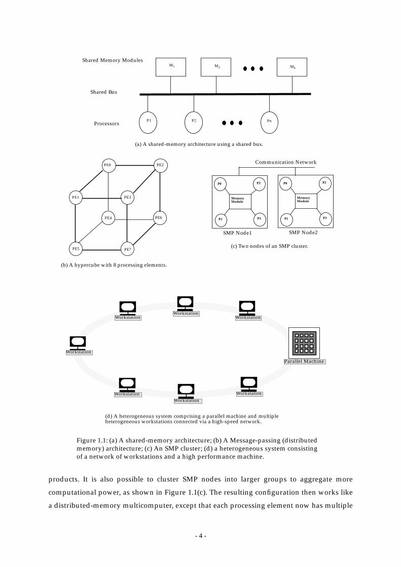
Figure 1.1: (a) A shared-memory architecture; (b) A Message-passing (distributed

memory) architecture; (c) An SMP cluster; (d) a heterogeneous system

consisting of a network of workstations and

a high performance machine. ............................................................................ 4

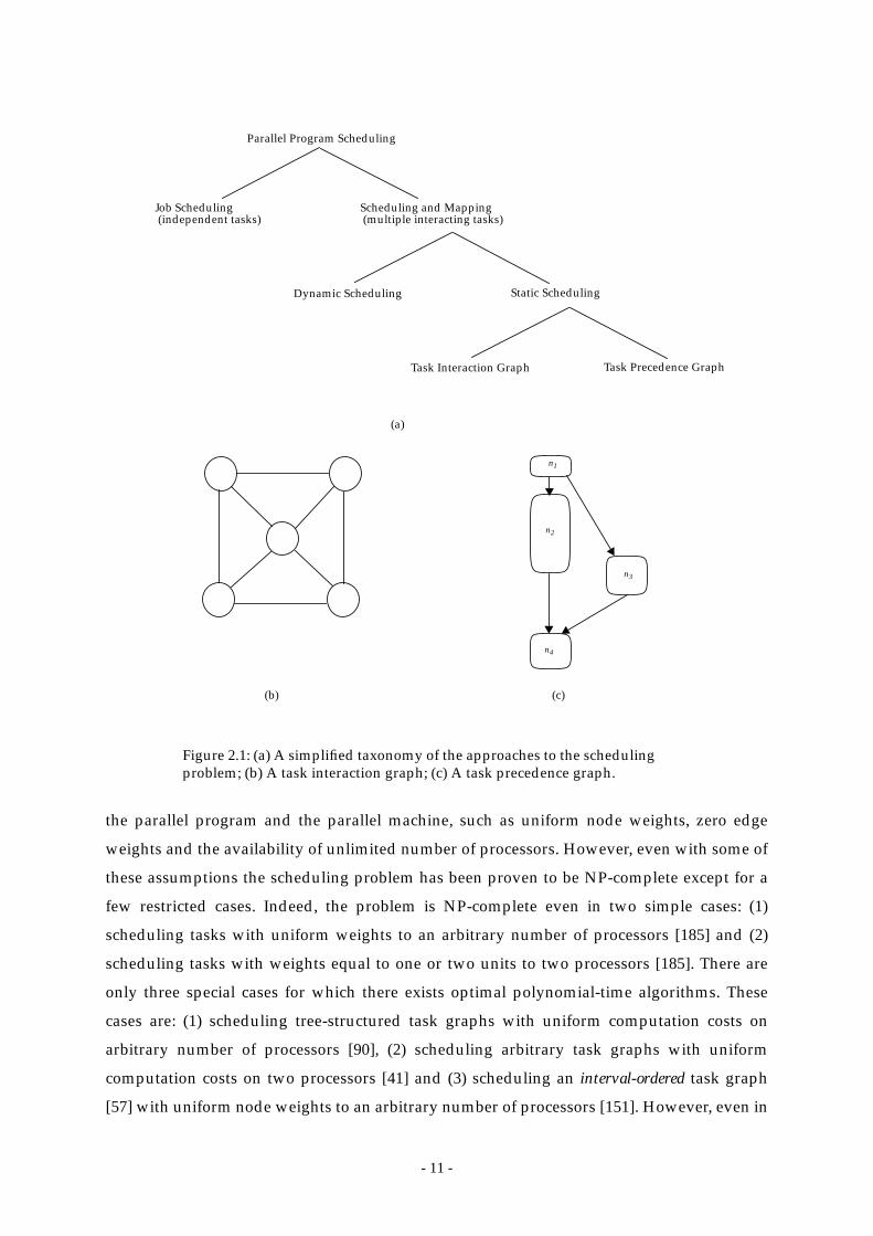
Figure 2.1: (a) A simplified taxonomy of the approaches to the scheduling problem; (b)

A task interaction graph; (c) A task precedence graph. .............................. 11

Figure 2.2: (a) A task graph; (b) The static levels (SLs), t-levels, b-levels and ALAPs of

the nodes............................................................................................................. 19

Figure 2.3: A partial taxonomy of the multiprocessor scheduling problem. ............... 21

Figure 2.4: (a) A simple tree-structured task graph with unit-cost tasks and without

communication among tasks; (b) The optimal schedule of the task graph

using three processors. ..................................................................................... 25

Figure 2.5: (a) A simple task graph with unit-cost tasks and without communication

among tasks; (b) The optimal schedule of the task graph in a two-processor

system. ................................................................................................................ 26

Figure 2.6: (a) A unit-computational interval ordered DAG. (b) An optimal schedule

of the DAG. ........................................................................................................ 27

Figure 2.7: (a) A fork set; and (b) a join set. ...................................................................... 31

Figure 2.8: (a) The schedule generated by the EZ algorithm (schedule length = 18); (b)

A scheduling trace of the EZ algorithm......................................................... 33

Figure 2.9: (a) The schedule generated by the LC algorithm (schedule length = 19); (b)

A scheduling trace of the LC algorithm......................................................... 34

Figure 2.10:(a) The schedule generated by the DSC algorithm (schedule length = 17);

(b) A scheduling trace of the DSC algorithm (N.C. indicates “not

considered”). ...................................................................................................... 35

- x -

Figure 2.11:(a) The schedule generated by the MD algorithm (schedule length = 17); (b)

A scheduling trace of the MD algorithm (N.C. indicates “not considered”,

N.R. indicates “no room”)................................................................................ 38

Figure 2.12:(a) The schedule generated by the DCP algorithm (schedule length = 16);

(b) A scheduling trace of the DCP algorithm (N.C. indicates “not

considered”, N.R. indicates “no room”). ....................................................... 39

Figure 2.13:(a) The schedule generated by the HLFET algorithm (schedule length =

19); (b) A scheduling trace of the HLFET algorithm (N.C. indicates “not

considered”). ...................................................................................................... 41

Figure 2.14:(a) The schedule generated by the ISH algorithm (schedule length = 19); (b)

A scheduling trace of the ISH algorithm (N.C. indicates “not

considered”). ...................................................................................................... 43

Figure 2.15:(a) The schedule generated by the MCP algorithm (schedule length = 20);

(b) A scheduling trace of the MCP algorithm (N.C. indicates “not

considered”). ...................................................................................................... 44

Figure 2.16:(a) The schedule generated by the ETF algorithm (schedule length = 19);

(b) A scheduling trace of the ETF algorithm (N.C. indicates “not

considered”). ...................................................................................................... 46

Figure 2.17:(a) The schedule generated by the DLS algorithm (schedule length = 19);

(b) A scheduling trace of the DLS algorithm (N.C. indicates “not

considered”). ...................................................................................................... 48

Figure 2.18:(a) The schedule generated by the LAST algorithm (schedule length = 19);

(b) A scheduling trace of the LAST algorithm (N.C. indicates “not

considered”). ...................................................................................................... 49

Figure 2.19:(a) The schedule generated by the PY algorithm (schedule length = 21); (b)

The e-values of the nodes computed by the PY algorithm. ........................ 53

Figure 2.20:(a) The schedule generated by the LWB algorithm (schedule length = 16);

(b) The lwb (lower bound) values of the nodes computed by the LWB

algorithm. ........................................................................................................... 54

Figure 2.21:(a) The schedule generated by the DSH algorithm (schedule length = 15);

- xi -

(b) A scheduling trace of the DSH algorithm................................................ 56

Figure 2.22:(a) The schedule generated by the LCTD algorithm (schedule length = 17);

(b) A scheduling trace of the LCTD algorithm. ............................................ 57

Figure 2.23:(a) The schedule generated by the CPFD algorithm (schedule length = 15);

(b) A scheduling trace of the CPFD algorithm.............................................. 61

Figure 2.24:The schedule generated by the MH and DLS algorithm (schedule length =

20, total comm. costs incurred = 16). .............................................................. 64

Figure 2.25:The schedule generated by the BU algorithm (schedule length = 24, total

comm. costs incurred = 27). ............................................................................. 66

Figure 2.26:Intermediate schedules produced by BSA after (a) serial injection

(schedule length = 30, total comm. cost = 0); (b) n4 migrates from PE 0 to PE

1 (schedule length = 26, total comm. cost = 2); (c) n3 migrates from PE 0 to

PE 3 (schedule length = 23, total comm. cost = 4); (d) n8 migrates from PE

0 to PE 1 (schedule length = 22, total comm. cost = 9). ................................ 68

Figure 2.27:(a) Intermediate schedule produced by BSA after n6 migrates from PE 0 to

PE 3 (schedule length = 22, total comm. cost = 15); (b) final schedule

produced by BSA after n9 migrates from PE 0 to PE 1 and n5 is bubbled up

(schedule length = 16, total comm. cost = 21). .............................................. 69

Figure 3.1: (a) A task graph; (b) The static levels (SLs), t-levels (ASAP times), b-levels,

and ALAP times of the nodes (CPNs are marked by an asterisk). ............ 84

Figure 3.2: The schedule of the DAG in Figure 3.1 generated by (a) the MD algorithm;

(b) the ETF and DLS algorithms; (c) the DSC algorithm; (d) the procedure

InitialSchedule(); and (e) the random search process in the FAST

algorithm. ........................................................................................................... 85

Figure 3.3: Average normalized schedule lengths of the FAST algorithms for random

task graphs with 1000 nodes with various values of MAXSTEP and

MAXCOUNT. .................................................................................................... 86

Figure 3.4: The system organization of CASCH. ............................................................. 87

Figure 3.5: Normalized execution times, number of processors used, and scheduling

- xii -

algorithm running times for the Gaussian elimination for all the scheduling

algorithms........................................................................................................... 88


algorithm running times for the Laplace equation solver for all the

scheduling algorithms. ..................................................................................... 89


algorithm running times for FFT for all the scheduling algorithms.......... 90

Figure 3.8: (a) The average running times of the PFAST algorithm for the type-1

random task graphs with three CCRs using 1 PPE on the Intel Paragon; (b)

the average speedups of the PFAST algorithm for 2, 4, 8, and 16 PPEs.... 93

Figure 3.9: (a) The average running times of the PFAST algorithm for the type-2

random task graphs with three CCRs using 1 PPE on the Intel Paragon; (b)

the average speedups of the PFAST algorithm for 2, 4, 8, and 16 PPEs.... 94

Figure 3.10:Normalized schedule lengths and scheduling times for the large DAGs for

all the scheduling algorithms. ......................................................................... 95

Figure 4.1: Examples of the standard (a) crossover operator; (b) mutation operator;

and (c) inversion operator on a binary coded chromosome. .................... 102

Figure 4.2: The schedule generated by the start-time minimization method (schedule

length = 16 time units). ................................................................................... 107

Figure 4.3: Examples of the (a) order crossover, (b) PMX crossover, (c) cycle crossover,

and (d) mutation operators............................................................................ 109

Figure 4.4: (a) A simple task graph; (b) An example of generating an invalid ordering

of the graph by using the PMX crossover operator; (c) An example of

generating an invalid ordering of the graph by using the cycle crossover

operator............................................................................................................. 110

Figure 4.5: (a) The average running times of the PGS algorithm for the type-1 random

task graphs with three CCRs using 1 PPE on the Intel Paragon; (b) the

average speedups of the PGS algorithm for 2, 4, 8, and 16 PPEs. ............ 118

Figure 4.6: The average percentage deviations from the optimal of the solutions

- xiii -

generated by the PGS algorithm for the type-1 random task graphs with

three CCRs using 8 PPEs on the Intel Paragon. .......................................... 118

Figure 4.7: (a) The average running times of the PGS algorithm for the type-2 random

task graphs with three CCRs using 1 PPE on the Intel Paragon; (b) the

average speedups of the PGS algorithm for 2, 4, 8, and 16 PPEs. ............ 119

Figure 4.8: The average percentage deviations from the optimal of the solutions

generated by the PGS algorithm for the type-2 random task graphs with

three CCRs using 8 PPEs on the Intel Paragon. .......................................... 120

Figure 4.9: (a) The average running times of the PGS algorithm for all the regular task

graphs with three CCRs using 1 PPE on the Intel Paragon; (b) the average

speedups of the PGS algorithm over the DSC algorithm; (c) the average

speedups of the PGS algorithm over the DCP algorithm. ........................ 124

Figure 4.10:The average ratios of schedule lengths for all the regular task graphs with

three CCRs using 8 PPEs on the Intel Paragon: (a) PGS vs. DSC and (b) PGS

vs. DCP. ............................................................................................................ 125

Figure 5.1: (a) A task graph; (b) The static levels (SLs) and the CPN-Dominant

sequence of the nodes..................................................................................... 138

Figure 5.2: (a) Intermediate schedule produced by BSA after serial injection (schedule

length = 300, total comm. cost = 0); (b) Intermediate schedule after n4, n3,

n8 are migrated (schedule length = 220, total comm. cost = 90); (c)

Intermediate schedule after n6 is migrated (schedule length = 220, total

comm. cost = 150); (d) final schedule after n9 is migrated (schedule length

= 160, total comm. cost = 160)........................................................................ 139

Figure 5.3: (a) The randomly generated task execution times on the heterogeneous

processors; (b) Intermediate schedule produced by BSA after serial

injection (schedule length = 238, total comm. cost = 0); (c) Intermediate

schedule after n3, n4, and n7 are migrated (schedule length = 218, total

comm. cost = 110); (d) Intermediate schedule after n8 and n9 are migrated

(schedule length = 147, total comm. cost = 200); (e) final schedule after n3

is migrated (schedule length = 138, total comm. cost = 200). ................... 140

Figure 5.4: (a) Computations of the EPFTs of the RPNs n1, n2, n3, n4, n6 and n7 based

- xiv -

on the processing times for PE 1; (b) Computations of the LPFTs of the

RPNs; (c) The estimated values of the RPNs............................................... 141

Figure 5.5: (a) The schedule of the first partition; (b) The schedule of the second

partition; (c) The schedule of the third partition; (d) The combined final

schedule generated by the PBSA algorithm (schedule length = 146, total

comm. costs incurred = 110). ......................................................................... 142

Figure 5.6: (a) Average schedule length ratios of the PBSA algorithm to the BSA

algorithm; (b) Average speedups of PBSA with respect to BSA for regular

graphs; (c) Average speedups of PBSA with respect to BSA for random

graphs. .............................................................................................................. 150

Figure 5.7: (a) Average schedule length ratios of the PBSA algorithm to the MH

algorithm; (b) Average speedups of PBSA over MH for regular graphs; (c)

Average speedups of PBSA over MH for random graphs........................ 151

Figure 5.8: (a) Average schedule length ratios of the PBSA algorithm to the DLS

algorithm; (b) Average speedups of PBSA over DLS for regular graphs; (c)

Average speedups of PBSA over DLS for random graphs. ...................... 152

Figure 5.9: (a) Average schedule length ratios of the PBSA algorithm to the BU

algorithm; (b) Average speedups of PBSA over BU for regular graphs; (c)

Average speedups of PBSA over BU for random graphs. ........................ 153

Figure 5.10:The effect of parameter on schedule length........................................... 154α

- xv -

List of Tables

Table 2.1: Summary of optimal scheduling under various simplified situations. .... 17

Table 2.2: Some of the well known scheduling algorithms and

their characteristics. .......................................................................................... 24

Table 3.1: Results of the PFAST algorithm compared against optimal solutions

(percentage deviations) for the type-1 random task graphs with three CCRs

using 1, 2, 4, 8, and 16 PPEs on the Intel Paragon. ....................................... 92

Table 3.2: Results of the PFAST algorithm compared against optimal solutions


using 1, 2, 4, 8, and 16 PPEs on the Intel Paragon. ....................................... 94

Table 4.1: The percentage deviations from optimal schedule lengths for the type-1

random task graphs with three CCRs using four values of population-size

constant: kp = 2, 3, 5, and 10; 8 PPEs were used for all the cases............. 116

Table 4.2: The percentage deviations from optimal schedule lengths for the type-1

random task graphs with three CCRs using four values of number-of-

generation constant: kg = 2, 5, 10, and 20; 8 PPEs were used for all the

cases................................................................................................................... 116

Table 4.3: Results of the PGS algorithm compared against optimal solutions


using 2, 4, 8, and 16 PPEs on the Intel Paragon. ......................................... 117

Table 4.4: Results of the PGS algorithm compared against optimal solutions



Table 4.5: Ratios of the schedule lengths generated by the PGS algorithm to that of the

DSC algorithm for the Gaussian elimination task graphs with three CCRs



- xvi -

DCP algorithm for the Gaussian elimination task graphs with three CCRs



DSC algorithm for the LU-decomposition task graphs with three CCRs



DCP algorithm for the LU-decomposition task graphs with three CCRs



DSC algorithm for the Laplace equation solver task graphs with three

CCRs using 2, 4, 8, and 16 PPEs on the Intel Paragon. .............................. 123


DCP algorithm for the Laplace equation solver task graphs with three

CCRs using 2, 4, 8, and 16 PPEs on the Intel Paragon. .............................. 123

Table 5.1: Ratios of schedule lengths generated by the MH, DLS, BU and PBSA (using

16 PPEs) algorithms for Cholesky factorization task graphs on four target

topologies. ........................................................................................................ 144


16 PPEs) algorithms for Gaussian elimination task graphs on four target

topologies. ........................................................................................................ 146


16 PPEs) algorithms for FFT task graphs

on four target topologies. ............................................................................... 147


16 PPEs) algorithms for random task graphs

on four target topologies. ............................................................................... 148

Table 5.5: Average running times of the MH, DLS, BU, BSA and PBSA (using 16 PPEs)

algorithms for various task graphs across all CCRs

and target topologies. ..................................................................................... 149

Table 5.6: Ratios of the schedule length produced by the PBSA algorithm to that of the

- xvii -

BSA algorithm for random task graphs of various sizes on a 4x2 mesh with

heterogeneous processors. ............................................................................. 152

- xviii -

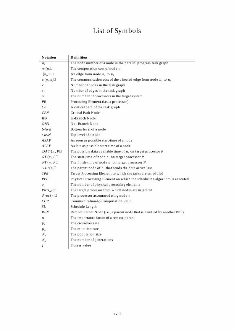
List of Symbols

Notation Definition

The node number of a node in the parallel program task graph

The computation cost of node

An edge from node to

The communication cost of the directed edge from node to

v Number of nodes in the task graph

e Number of edges in the task graph

p The number of processors in the target system

PE Processing Element (i.e., a processor)

CP A critical path of the task graph

CPN Critical Path Node

IBN In-Branch Node

OBN Out-Branch Node

b-level Bottom level of a node

t-level Top level of a node

ASAP As soon as possible start-time of a node

ALAP As late as possible start-time of a node

The possible data available time of on target processor P

The start-time of node on target processor P

The finish-time of node on target processor P

The parent node of that sends the data arrive last

TPE Target Processing Element to which the tasks are scheduled

PPE Physical Processing Element on which the scheduling algorithm is executed

q The number of physical processing elements

Pivot_PE The target processor from which nodes are migrated

The processor accommodating node

CCR Communication-to-Computation Ratio

SL Schedule Length

RPN Remote Parent Node (i.e., a parent node that is handled by another PPE)

The importance factor of a remote parent

The crossover rate

The mutation rate

The population size

The number of generations

Fitness value

ni

w ni( ) ni

ni nj,( ) ni nj

c ni nj,( ) ni nj

DAT ni P,( ) ni

ST ni P,( ) ni

FT ni P,( ) ni

VIP ni( ) ni

Proc ni( ) ni

αµc

µm

Np

Ng

f

- xix -


By

Yu-Kwong KWOKA Thesis Presented to

Department of Computer Science, The Hong Kong University of Science and Technology, Hong KongMay 1997

Abstract

Scheduling and mapping of precedence-constrained task graphs to the processors is oneof the most crucial problems in parallel and distributed computing and thus continues tospur a great deal of interest from the researchers. Due to the NP-completeness of the problem,a large portion of related work is based on heuristic approaches with the objective of findinggood solutions within a reasonable amount of time. The major drawback with most of theexisting heuristics, however, is that they are evaluated with small problems sizes and thustheir scalability is unknown. As a result, they are not applicable in a real environment whenpresented with moderately large problems. Furthermore, most heuristics ignore theimportant details of the application and the target system, or do not perform well when thesedetails are taken into account. In this research, we propose three scheduling algorithms forachieving the conflicting goals of high-performance and low time-complexity. In addition, weaim at making our algorithms scalable and applicable when used in a real environment. Thenovelty of our algorithms is their efficient scheduling strategies which yield better solutionswithout incurring a high complexity. The second novelty is that our algorithms areparallelized which further lowers their complexities. The first algorithm, called the Parallel

Fast Assignment using Search Technique (PFAST) algorithm, is a linear-time algorithm and usesan effective neighborhood search strategy for finding a good solution in a short time. ThePFAST algorithm constructs an initial solution using a fast heuristic and then refines thesolution using a parallel random search. The second algorithm, called the Parallel Genetic

Search (PGS) algorithm, employs a parallel genetic technique which is based on the premisesthat the recombinative nature of a genetic algorithm can potentially determine an optimalschedule. Using well-defined crossover and mutation operators, the PGS algorithmjudiciously combines good building-blocks of potential solutions to move towards a bettersolution. The third algorithm, called the Parallel Bubble Scheduling and Allocation (PBSA)algorithm, is applicable in a general distributed computing environment in that it takes intoaccount more considerations such as link contention, heterogeneity of processors, and thenetwork topology. The PBSA algorithm uses an efficient strategy for simultaneousscheduling of tasks and messages. The algorithm is parallelized by partitioning the taskgraph to smaller graphs, finding their sub-schedules concurrently, and then combining thesesub-schedules. The proposed algorithms have been evaluated through extensiveexperimentations and yield consistently better performance when compared with numerousexisting algorithms.

- 1 -

Chapter 1

Introduction

1.1 Overview

Parallel processing is a promising approach to meet the computational requirements of

the Grand Challenge problems [92], [168] or to enhance the efficiency of solving emerging

applications [110], [155]. However, it poses a number of problems which are not encountered

in sequential processing including designing a parallel algorithm for the application,

partitioning of the application into tasks, coordinating communication and synchronization,

and scheduling of the tasks onto the machine. If these problems are not properly handled,

parallelization of an application may not be beneficial. For example, if the tasks of an

application are not properly scheduled to the machine, the extra inter-task communication

overhead can offset the gain from parallelization. A large body of research efforts addressing

these problems has been reported in the literature [15], [28], [38], [65], [81], [92], [123], [129],

[130], [131], [153], [155], [164], [189], [192]. Our research focus is on the scheduling aspect.

The objective of scheduling is to minimize the completion time of a parallel application

by properly allocating the tasks to the processors and sequencing the execution of the tasks.

In a broad sense, the scheduling problem exists in two forms: static and dynamic. In static

scheduling, which is also referred to as compile-time scheduling, the characteristics of a

parallel program, including task processing times, data dependencies and synchronizations,

are known before program execution [28], [38], [65]. A parallel program, therefore, can be

represented by a node- and edge-weighted directed acyclic graph (DAG), in which the node

weights represent task processing times and the edge weights represent data dependencies as

well as the length of communication time. In dynamic scheduling, few assumptions about

the parallel program can be made before execution, and thus, scheduling decisions have to be

made on-the-fly [3], [94]. The goal of a dynamic scheduling algorithm as such includes not

only the minimization of the program completion time but also the minimization of

scheduling overhead, which represents a significant portion of the cost paid for running the

scheduler. We address only the static scheduling problem. Hereafter we refer to the static

- 2 -

scheduling problem as simply scheduling.

The scheduling problem is NP-complete for most of its variants except for a few highly

simplified cases (these cases will be elaborated in Chapter 2) [37], [40], [41], [51], [52], [63],

[74], [78], [90], [100], [150], [151], [152], [158], [162], [185], and therefore, many heuristics with

polynomial-time complexity have been suggested [8], [9], [31], [40], [51], [52], [66], [102],

[134], [147], [154], [165], [174]. However, most of these heuristics are based on simplifying

assumptions about the structure of the parallel program and the target parallel architecture,

and thus are not useful in practical situations.

Common simplifying assumptions include uniform task execution times, zero inter-task

communication times, contention-free communication, full connectivity of parallel

processors, and availability of unlimited number of processors. These assumptions are not

valid in practical situations for a number of reasons. For one thing, it is not realistic to assume

that the task execution times of an application are uniform no matter whether data

parallelism or functional parallelism is exploited because the amount of computation

encapsulated in a task is usually varied. Furthermore, other simplifying assumptions are

usually not valid for modern parallel machines such as distributed-memory multicomputers

(DMMs) [92], shared-memory multiprocessors (SMMs) [92], clusters of symmetric

multiprocessors (SMPs) [155], and networks of workstations (NOWs) [92]. First, inter-task

communication in the form of message-passing or shared-memory access inevitably incurs a

non-negligible amount of latency. Second, contention-free communication and full

connectivity of processors are impossible for a DMM, a SMP or a NOW, and are hardly

achievable even in a SMM. Finally, relative to the size of a parallel application in terms of the

number of tasks [10], the number of processors in most parallel machines, which may be

thousands [92], is nonetheless limited. Thus, a scheduling algorithm relying on such

assumptions is apt to have restricted applicability in real environments.

To be applicable in a practical environment, a scheduling algorithm needs to address a

number of challenging issues. It should exploit parallelism by identifying the task graph

structure, and take into consideration task granularity, load balancing, arbitrary task weights

and communication costs, the number of target processors available, and the scheduling of

inter-processor communication. For example, to model link contention, messages have to be

properly scheduled to the communication links. To properly handle message scheduling, the

processor network topology should also be considered. To give good performance while

taking into account all of these aspects can produce a scheduling algorithm with very high

time-complexity. High complexity in turn limits scalability. For instance, many heuristics

- 3 -

have been evaluated with small task graphs and thus their scalability is not known. It is not

clear whether they can yield good solutions within reasonable time for large task graphs

found in many real-world problems [10]. On the other hand, to be of practical use, a

scheduling algorithm should be fast. These conflicting requirements make the design of an

efficient scheduling algorithm more intricate and challenging.

1.2 Parallel Architectures and The Scheduling Problem

Parallel processing platforms exist in a wide variety of forms [49], [84], [167]. The most

common forms are the shared-memory (Figure 1.1(a)) and message-passing (distributed

memory) (Figure 1.1(b)) architectures. Shared-memory machines (e.g., the BBN Butterfly [49],

the KSR-1 [92] and KSR-2 [92]) present a uniform-address-space view of the memory to the

programmer and therefore, interprocessor communication is accomplished through writing

and reading of shared variables. The hardware generally provides an “equal-cost” access to

any shared variable from any of the processors and there is no notion of communication

locality. The major advantage of shared-memory architectures is that program development

is relatively easy. Message-passing architectures (e.g., Intel iPSC hypercubes [84], Intel

Paragon meshes [92], and CM-5 [92]) use direct communication links between processors and

therefore, interprocessor communication and synchronization are achieved through explicit

message-passing. In a message-passing architecture, each processing element (PE) is

composed of a processor and a local memory, and is connected to a fixed number of PEs in

some regular topology such as a ring or a hypercube (see Figure 1.1(b)) [166], [170]. The

advantage of this approach over the shared-memory approach is the greater communication

bandwidth in the system, due to the large number of simultaneous communications possible

on the independent interprocessor links. Another advantage is scalability. One can add new

PEs as well as communication channels to a message-passing multicomputer at a very low

cost. The disadvantage is the longer communication delay when the destination PE is not

directly connected to the source PE. This problem has recently been alleviated by employing

a new message switching technique called the worm-hole routing [43]. However, the

message set-up time remains a significant overhead in PE communications.

Recently the symmetric multiprocessor (SMP) machines has joined the parallel machines

marketplace. They are designed using workstation microprocessor technology, but with

several CPUs coupled together with a small shared memory in each SMP node. The term

“symmetric” means that each CPU can retrieve data stored at a given memory location in the

same amount of time. Each SMP node closely resemble a shared-memory multiprocessor, but

is slower and less expensive. Examples include SGI’s PowerChallenge and Sun’s SparcServer

- 4 -

products. It is also possible to cluster SMP nodes into larger groups to aggregate more

computational power, as shown in Figure 1.1(c). The resulting configuration then works like

a distributed-memory multicomputer, except that each processing element now has multiple

Processors

Shared Memory Modules

P1 P2 Pn

M1 M2 Mk

(a) A shared-memory architecture using a shared bus.

PE0 PE2

PE1 PE3

PE5 PE7

PE6PE4

Figure 1.1: (a) A shared-memory architecture; (b) A Message-passing (distributedmemory) architecture; (c) An SMP cluster; (d) a heterogeneous system consistingof a network of workstations and a high performance machine.

(b) A hypercube with 8 processing elements.

Shared Bus

P0

P1 P3

P2

MemoryModule

SMP Node1

P0

P1 P3

P2

MemoryModule

SMP Node2

(c) Two nodes of an SMP cluster.

Communication Network

(d) A heterogeneous system comprising a parallel machine and multipleheterogeneous workstations connected via a high-speed network.

Parallel Machine

WorkstationWorkstation

Workstation

WorkstationWorkstation

Workstation

Workstation

- 5 -

CPUs sharing a common memory.

With the advanced networking and communication tools, heterogenous integrated

environments [167], as shown in Figure 1.1(d), connecting both high performance machines

and workstations are also viable choices for parallel processing.

To effectively harness the computing power of all these parallel architectures, optimized

scheduling of the parallel program tasks to the processors is crucial. Indeed, if the tasks of a

parallel program are not scheduled properly, the parallel program is likely to produce a poor

speedup which renders parallelization useless.

1.3 Research Objectives

In the design of our scheduling algorithms for efficient parallel processing, we address

four fundamental aspects: performance, time-complexity, scalability, and applicability. These

aspects are elaborated below.

Performance. We have designed high performance and robust scheduling algorithms. By

high performance we mean the scheduling algorithms produce high quality solutions. The

quality of the solutions are evaluated with respect to optimal solutions. While the proposed

algorithms are heuristic in nature, they give better performance than contemporary

algorithms in general. The algorithms are also robust in that they can be used under a wide

range of input parameters (e.g., arbitrary number of available target processors and diverse

task graph structures).

Time-complexity. We have designed our scheduling algorithms with low time-complexity

by parallelization of the algorithms. The time-complexity of an algorithm is an important

factor insofar as the quality of solution is not compromised. Parallelizing a scheduling

algorithm is a novel as well as natural way to reduce the time-complexity. This approach is

novel in that no previous work has been done in the parallelization of a scheduling

algorithm. And it is natural in that parallel processing is realized only when a parallel

processing platform is available. Furthermore, parallelization can be utilized not only to

speed up the scheduling process further but also to improve the solution quality.

Scalability. Our parallel scheduling algorithms are scalable. On the one hand, the

algorithms possess problem-size scalability, that is, the algorithms consistently give a good

performance even for large input. This is essential since, in practice, a task graph generated

from a numerical application can easily have a few thousands nodes [10]. On the other hand,

- 6 -

the algorithms possess processing-power scalability, that is, given more processors for a

problem, the parallel scheduling algorithms produce solutions with almost the same quality

in a shorter period of time.

Applicability. Our scheduling algorithms can be used in practical environments. To achieve

this goal, we take into account realistic assumptions about the program and multiprocessor

models such as arbitrary computation and communication weights, link contention, and

processor network topology. Moreover, the proposed algorithms have been evaluated using

real benchmarks generated by a parallel program compiler [10].

1.4 Contributions

The contributions of this thesis are as follows:

• A Low-Complexity Algorithm. We have developed a scheduling algorithm that takes

linear-time to generate solutions with high quality. We have compared the algorithm

with a number of well-known efficient scheduling algorithms and found that it

outperforms the other algorithms in terms of solution quality as well as speed. We have

also parallelized the algorithm to further reduce its running time. We have investigated

the performance of the parallel algorithm under a wide range of input and scheduling

parameters and found that it generates optimal solutions for a significant portion of the

test cases and close to optimal solutions for the others. Furthermore, its running times

are considerably shorter than other algorithms. The algorithm, called Parallel Fast

Assignment using Search Technique (PFAST) algorithm, can be used in a parallel

processing platform for producing high quality schedules under running time

constraint.

• Near-to-Optimal Scheduling using Parallel Genetic Search. We have developed a parallel

genetic-search-based scheduling algorithm which can potentially generate optimal

solutions. Genetic algorithms are global search techniques which explore different

regions of the search space by keeping track of a set of potential solutions of diverse

characteristics, called a population. As such, genetic search techniques can potentially

improve the quality of solutions when longer running time is affordable. In the

proposed genetic-search-based algorithm, we have used a novel encoding scheme, an

effective initial population generation strategy, and two computationally efficient

genetic search operators. We have evaluated the algorithm by extensive

experimentations and found that it generates optimal solutions for more than half of

the test cases and close-to-optimal solutions for the other half. Another merit of genetic

- 7 -

search is that its inherent parallelism can be exploited to further reduce its running

time. The proposed algorithm, called the Parallel Genetic Scheduling (PGS) algorithm,

can be used when close-to-optimal solutions are desired.

• A Parallel Algorithm for Scheduling in Unrestricted Environments. We have developed a

parallel algorithm for scheduling that is targetted for networked homogeneous or

heterogeneous systems. The design of the algorithm takes into account the

considerations such as limited number of processors, link contention, heterogeneity of

processors and processor network topology. The algorithm has been evaluated under a

board range of parameters: different number of processors, different types of

interconnection topology, different extents of processor heterogeneity, and different

task graph structures. In our experimental studies, we have found that the algorithm is

highly scalable in that it outperforms a number of other general scheduling algorithms

even for large task graphs. The proposed algorithm, called Parallel Bubble Scheduling

and Allocation (PBSA) algorithm, is applicable in a general distributed ocmputing

environment.

1.5 Organization of the Thesis

The organization of the thesis is as follows. In Chapter 2, we provide a detailed discussion

about the scheduling problem. To enable the reader to better understand the state of current

research, in the same chapter we also provide a brief literature survey, which is based on a

taxonomy of scheduling algorithms. In Chapter 3, we present the proposed Parallel Fast

Assignment using Search Technique (PFAST) algorithm. We first put forth the sequential

version of the algorithm, called the FAST algorithm, followed by the results and comparisons

with other fast scheduling algorithms. Finally we present the PFAST algorithm followed by

the experimental results. In Chapter 4, we present the proposed Parallel Genetic Scheduling

(PGS) algorithm. We first briefly review the basic ideas and mechanisms of genetic search

techniques, followed by a discussion about the parallelization issues of a genetic algorithm.

We then present a scrutiny of list scheduling techniques. This scrutiny motivates the

formulation of the scheduling problem in a genetic-search framework. Finally, we present the

PGS algorithm and its performance results. The PGS algorithm is also compared with the

PFAST algorithm. In Chapter 5, we present the proposed Parallel Bubble Scheduling and

Allocation (PBSA) algorithm. We discuss the target scheduling environments, followed by

the design principles of the PBSA algorithm. A small example is used to illustrate the

characteristics of the algorithm. Finally, performance results and a comparison with other

algorithms are presented. Last, in Chapter 6, we conclude with some final remarks and a brief

- 8 -

discussion of some future research directions.

- 9 -

Chapter 2

Background and Literature Survey

2.1 Introduction

To facilitate understanding the proposed algorithms and the state of current research on

scheduling, in this chapter we present the background of the scheduling problem and briefly

survey the representative work in the literature. Multiprocessors scheduling has been an

active research area since the notion of parallel processing was introduced. However, many

different assumptions and terminology are independently suggested. Unfortunately, some of

the terms, concepts, and assumptions are not clearly stated nor consistently used by most of

the researchers. As a result, it is difficult to appreciate the merits of various scheduling

algorithms and quantitatively evaluate the performance of the algorithms. To avoid this

problem, we first introduce the directed acyclic graph (DAG) model of a parallel program, and

then proceed to describe the multiprocessor model. This is followed by a discussion about the

NP-completeness of variants of the scheduling problem. Finally, some basic techniques used

in most scheduling algorithms are introduced. Based on the classification of different

scheduling environments, we describe a taxonomy of scheduling algorithms. We illustrate

the taxonomy by describing several recently reported algorithms and use some scheduling

examples to highlight the differences in the design of the algorithms.

Since the scheduling problem is of crucial importance to the effective utilization of large

scale parallel computers and distributed computer networks, many different forms of

scheduling have been studied. In a broad sense, the general scheduling problem can be

divided into two categories—job scheduling and scheduling and mapping (see Figure 2.1(a)). In

the former category, independent jobs are to be scheduled among the processors of a

distributed computing system to optimize overall system performance [29], [33], [36], [68]. In

contrast, the scheduling and mapping problem requires the allocation of multiple interacting

tasks of a single parallel program in order to minimize the completion time on the parallel

computer system [1], [8], [9], [18], [31], [40], [184]. While job scheduling requires dynamic

run-time scheduling that is not a priori decidable, the scheduling and mapping problem can

- 10 -

be addressed in both static [51], [52], [66], [85], [86], [102], [134], [165] as well as dynamic

contexts [3], [94], [145]. When the characteristics of the parallel program, including its task

execution times, task dependencies, task communications and synchronization, are known a

priori, scheduling can be accomplished offline during compile-time. On the contrary, dynamic

scheduling is required when a priori information is not available and scheduling is done on-

the-fly according to the state of the system. We consider only the static scheduling problem.

Two distinct models of the parallel program have been considered extensively in the

context of static scheduling—the task interaction graph (TIG) model and task precedence graph

(TPG) model. They are shown in Figure 2.1(b) and Figure 2.1(c).

The task interaction graph model, in which graph vertices represent parallel processes

and edges denote the inter-process interaction [25], is usually used in static scheduling of

loosely-coupled communicating processes to a distributed system. Since all tasks are

considered as simultaneously and independently executable, there are no temporal execution

dependency. For example, a TIG is commonly used to model the finite element method

(FEM) [24], [26], [28]. The objective of scheduling is to minimize parallel program completion

time by properly mapping the tasks to the processors [27], [119], [127]. This requires

balancing the computation load uniformly among the processors while simultaneously

keeping communication costs as low as possible. The research in this area was pioneered by

Stone and Bohkari [24], [26], [27], [28], [177]: Stone [177] applied network-flow algorithms to

solve the assignment problem while Bokhari described the mapping problem as being

equivalent to graph isomorphism, quadratic assignment and sparse matrix bandwidth

reduction problems [25].

The task precedence graph model, in which the nodes represent the tasks and the directed

edges represent the execution dependencies as well as the amount of communication, is

commonly used in static scheduling of a parallel program with tightly-coupled tasks to

multiprocessors. For example, in the task precedence graph shown in Figure 2.1(c), task n4

cannot commence execution before tasks n1 and n2 finish execution and gathers all the

communication data from n2 and n3. The scheduling objective is to minimize the program

completion time or maximize the speed-up, defined as the time required for sequential

execution divided by the time required for parallel execution. For most parallel applications,

a task precedence graph can model the program more accurately because it captures the

temporal dependencies among tasks. This is the model we use in our research.

Earlier static scheduling research made simplifying assumptions about the architecture of

- 11 -

the parallel program and the parallel machine, such as uniform node weights, zero edge

weights and the availability of unlimited number of processors. However, even with some of

these assumptions the scheduling problem has been proven to be NP-complete except for a

few restricted cases. Indeed, the problem is NP-complete even in two simple cases: (1)

scheduling tasks with uniform weights to an arbitrary number of processors [185] and (2)

scheduling tasks with weights equal to one or two units to two processors [185]. There are

only three special cases for which there exists optimal polynomial-time algorithms. These

cases are: (1) scheduling tree-structured task graphs with uniform computation costs on

arbitrary number of processors [90], (2) scheduling arbitrary task graphs with uniform

computation costs on two processors [41] and (3) scheduling an interval-ordered task graph

[57] with uniform node weights to an arbitrary number of processors [151]. However, even in

Parallel Program Scheduling

Job Scheduling (independent tasks)

Scheduling and Mapping (multiple interacting tasks)

Dynamic Scheduling Static Scheduling

Task Interaction Graph Task Precedence Graph

n2

n1

n3

n4

(a)

(b) (c)

Figure 2.1: (a) A simplified taxonomy of the approaches to the schedulingproblem; (b) A task interaction graph; (c) A task precedence graph.

- 12 -

these cases, communication among tasks of the parallel program is assumed to take zero time

[40]. Given these observations, it is unlikely that the general scheduling problem can be

solved in polynomial-time, unless .

Due to the intractability of the general scheduling problem, two distinct approaches have

been taken: sacrificing efficiency for the sake of optimality and sacrificing optimality for the

sake of efficiency. To obtain optimal solutions under relaxed constraints, state-space search

and dynamic programming techniques have been suggested. However, these techniques are

not useful because most of them are designed to work under restricted environments and

most importantly they incur an exponential time in the worst case. In view of the

ineffectiveness of optimal techniques, many heuristics have been suggested to tackle the

problem under more pragmatic situations. While these heuristics are shown to be effective in

experimental studies, they usually cannot generate optimal solutions, and there is no

guarantee about their performance in general. Most of the heuristics are based on a list

scheduling approach [40], which is explained below.

The basic idea of list scheduling is to make a scheduling list (a sequence of nodes for

scheduling) by assigning them some priorities, and then repeatedly execute the following

two steps until all the nodes in the graph are scheduled:

1) Remove the first node from the scheduling list.

2) Allocate the node to a processor which allows the earliest start-time.

There are various ways to determine the priorities of nodes such as HLF (Highest level

First) [40], LP (Longest Path) [40], LPT (Longest Processing Time) [74] and CP (Critical Path)

[78].

Recently a number of scheduling algorithms based on a dynamic list scheduling approach

have been suggested [114], [172], [193]. In a traditional scheduling algorithm, the scheduling

list is statically constructed before node allocation begins, and most importantly the

sequencing in the list is not modified. In contrast, after each allocation, these recent

algorithms re-compute the priorities of all unscheduled nodes which are then used to

rearrange the sequencing of the nodes in the list. Thus, these algorithms essentially employ

the following three-step approaches:

1) Determine new priorities of all unscheduled nodes.

2) Select the node with the highest priority for scheduling.

3) Allocate the node to the processor which allows the earliest start-time.

P NP=

- 13 -

Scheduling algorithms which employ this three-step approach can potentially generate

better schedules. However, a dynamic approach can increase the time-complexity of the

scheduling algorithm.

There are a number of other variations of scheduling algorithms designed for particular

target parallel processing environments. These variations include algorithms based on task-

duplication technique and algorithms for scheduling tasks to processors connected by a

particular topology in which link contention has to be considered. We survey representative

work in these various categories. Examples are used to illustrate their difference in design.

The organization of this chapter is as follows. In Section 2.2 we provide the problem

statement and describe in detail the DAG model and the multiprocessor model used in our

study. In Section 2.3 we describe the optimality and NP-completeness of the various

simplified cases of the problem. In Section 2.4 we describe and explain a set of basic

techniques commonly used in most scheduling algorithms. In Section 2.5 we propose a

taxonomy of the scheduling algorithms which is useful for understanding the different

characteristics and assumptions of different algorithms. In Section 2.6 we apply the proposed

taxonomy by presenting a survey of contemporary scheduling algorithms and analytical

results relating to the theoretical performance of some algorithms. Small examples are given

to illustrate the design of the surveyed algorithms. The final section summarizes this chapter.

2.2 Problem Statement and The Models Used

The objective of scheduling is to minimize the overall program finish-time by proper

allocation of the tasks to the processors and arrangement of execution sequencing of the

tasks. Scheduling is done in such a manner that the precedence constraints among the

program tasks are not violated. An important implication of minimization of program finish-

time is that the system throughput is maximized. This is because minimization of the overall

finish-time of every parallel program increases the number of parallel programs that can be

processed per unit of time. The overall finish-time of a parallel program is commonly called

the schedule length or makespan.

In the literature, there have been some variations to this goal. For example, some

researchers proposed algorithms to minimize the mean flow-time or mean finish-time, which is

the average of the finish-times of all the program tasks [30], [122]. The significance of the

mean finish-time criterion is that minimizing it in the final schedule leads to the reduction of

the mean number of unfinished tasks at each point in the schedule. There are also some other

- 14 -

algorithms proposed to reduce the setup costs of the parallel processors [178]. We focus on

algorithms for minimizing schedule length.

2.2.1 The DAG Model

In static scheduling, a parallel program can be represented by a directed acyclic graph

(DAG) , where V is a set of v nodes and E is a set of e directed edges. A node in

the DAG represents a task which in turn is a set of instructions which must be executed

sequentially without preemption in the same processor. The weight of a node is called the

computation cost and is denoted by . The edges in the DAG, each of which is denoted by

, correspond to the communication messages and precedence constraints among the

nodes. The weight of an edge is called the communication cost of the edge and is denoted by

. The source node of an edge is called the parent node while the sink node is called

the child node. A node with no parent is called an entry node and a node with no child is

called an exit node. The communication-to-computation-ratio (CCR) of a parallel program is

defined as its average edge weight divided by its average node weight. Hereafter we use the

terms node and task interchangeably.

The precedence constraints of a DAG dictate that a node cannot start execution before it

gathers all of the messages from its parent nodes. The communication cost between two tasks

assigned to the same processor is assumed to be zero. If node is scheduled to some

processor, then and denote the start-time and finish-time of , respectively.

After all the nodes have been scheduled, the schedule length is defined as

across all processors. The goal of scheduling is to minimize .

The node and edge weights are usually obtained by estimation at compile-time [10], [38],

[189]. Generation of the generic DAG model and some of the variations are described below.

2.2.2 DAG Generation

A parallel program can be modeled by a DAG. Although program loops cannot be

explicitly represented by the DAG model, data-flow computations parallelism in loops can be

exploited to subdivide the loops into a number of tasks by the loop-unraveling technique [20],

[120]. The idea is that all iterations of the loop are started or fired together, and operations in

various iterations can execute when their input data are ready for access. In addition, for a

large class of data-flow computation problems and most of the numerical algorithms (such as

matrix multiplication), there are very few, if any, conditional branches or indeterminism in

the program. Thus, the DAG model can be used to accurately represent these applications so

G V E,( )=

ni

w ni( )

ni nj,( )

c ni nj,( )

ni

ST ni( ) FT ni( ) ni

maxi FT ni( ){ }

maxi FT ni( ){ }

- 15 -

that the scheduling techniques can be applied. Furthermore, in many numerical applications,

such as Gaussian elimination or fast Fourier transform (FFT), the loop bounds are known

during compile-time. As such, one or more iterations of a loop can be deterministically

encapsulated in a task and, consequently, be represented by a node in a DAG.

The node- and edge-weights are usually obtained by estimation using profiling

information of operations such as numerical operations, memory access operations, and

message-passing primitives [97].

2.2.3 Variations of the DAG Model

There are a number of variations of the generic DAG model described above. The more

important variations are: preemptive scheduling vs. non-preemptive scheduling, parallel tasks vs.

non-parallel tasks and DAG with conditional branches vs. DAG without conditional branches.

Preemptive Scheduling vs. Non-preemptive Scheduling: In preemptive scheduling, the

execution of a task may be interrupted so that the unfinished portion of the task can be re-

allocated to a different processor [34], [75], [88], [157]. On the contrary, algorithms assuming

non-preemptive scheduling must allow a task to execute until completion on a single

processor. From a theoretical perspective, a preemptive scheduling approach allows more

flexibility for the scheduler so that a higher utilization of processors may result. Indeed, a

preemptive scheduling problem is commonly reckoned as “easier” than its non-preemptive

counterpart in that there are cases in which polynomial time solutions exist for the former

while the latter is proved to be NP-complete [40], [74]. However, in practice, interrupting a

task and transferring it to another processor can lead to significant processing overhead and

communication delays. In addition, a preemptive scheduler itself is usually more

complicated since it has to consider when to split a task and where to insert the necessary

communication induced by the splitting. We concentrate on the non-preemptive approaches.

Parallel Tasks vs. Non-parallel Tasks: A parallel task is a task that requires more than one

processor at the same time for its execution [187]. Blazewicz et al. investigated the problem of

scheduling a set of independent parallel tasks to identical processors under preemptive and

non-preemptive scheduling assumptions [22], [23]. Du and Leung also explored the same

problem but with one more flexibility: a task can be scheduled to no more than a certain pre-

defined maximum number of processors [48]. However, in Blazewicz et al. ‘s approach, a task

must be scheduled to a fixed pre-defined number of processors. Wang and Cheng further

extended the model to allow precedence constraints among tasks [187]. They devised a list

scheduling approach to construct a schedule based on the earliest completion time (ECT)

- 16 -

heuristic. We concentrate on scheduling DAGs with non-parallel tasks.

DAG with Conditional Branches vs. DAG without Conditional Branches: Towsley [182]

addressed the problem of scheduling a DAG with probabilistic branches and loops to

heterogeneous distributed systems. Each edge in the DAG is associated with a non-zero

probability that the child will be executed immediately after the parent. He introduced two

algorithms based on the shortest path method for determining the optimal assignments of

tasks to processors. El-Rewini and Ali [53] also investigated the problem of scheduling DAGs

with conditional branches. Similar to Towsley’s approach, they also used a two-step method

to construct a final schedule. However, unlike Towsley’s model, they modelled a parallel

program by using two DAGs: a branch graph and a precedence graph. This model differentiates

the conditional branching and the precedence relations among the parallel program tasks.

The objective of the first step of the algorithm is to reduce the amount of indeterminism in the

DAG by capturing the similarity of different instances of the precedence graph. After this

pre-processing step, a reduced branch graph and a reduced precedence graph are generated.

In the second step, all the different instances of the precedence graph are generated according

to the reduced branch graph, and the corresponding schedules are determined. Finally, these

schedules are merged to produce a unified final schedule. Since modelling branching and

looping in DAGs is an inherently difficult problem, few work has been reported in this area.

We concentrate on DAGs without conditional branching in this research.

2.2.4 The Multiprocessor Model

In DAG scheduling, the target system is assumed to be a network of processing elements

(PEs), each of which is composed of a processor and a local memory unit so that the PEs do

not share memory and communication relies solely on message-passing. The processors may

be heterogeneous or homogeneous. Heterogeneity of processors means the processors have

different speeds or processing capabilities. However, we assume every module of a parallel

program can be executed on any processor even though the completion times on different

processors may be different. The PEs are connected by an interconnection network of a

certain topology. The topology may be fully-connected or of a particular structure such as a

hypercube or mesh. Although processors may be heterogeneous, we assume the

communication links are homogeneous, that is, a message is transmitted with the same speed

on all links.

2.3 NP-Completeness of the Scheduling Problem

The problem of optimally scheduling a DAG in polynomial-time has been solved for only

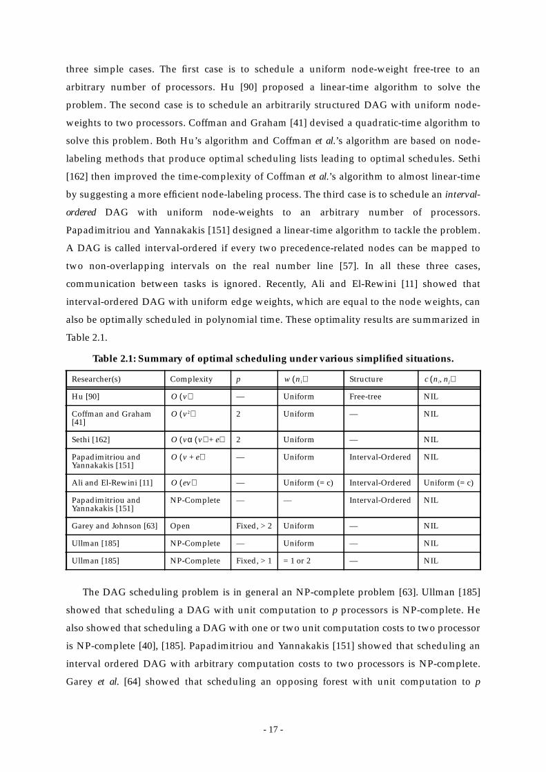
- 17 -

three simple cases. The first case is to schedule a uniform node-weight free-tree to an

arbitrary number of processors. Hu [90] proposed a linear-time algorithm to solve the

problem. The second case is to schedule an arbitrarily structured DAG with uniform node-

weights to two processors. Coffman and Graham [41] devised a quadratic-time algorithm to

solve this problem. Both Hu’s algorithm and Coffman et al.’s algorithm are based on node-

labeling methods that produce optimal scheduling lists leading to optimal schedules. Sethi

[162] then improved the time-complexity of Coffman et al.’s algorithm to almost linear-time

by suggesting a more efficient node-labeling process. The third case is to schedule an interval-

ordered DAG with uniform node-weights to an arbitrary number of processors.

Papadimitriou and Yannakakis [151] designed a linear-time algorithm to tackle the problem.

A DAG is called interval-ordered if every two precedence-related nodes can be mapped to

two non-overlapping intervals on the real number line [57]. In all these three cases,

communication between tasks is ignored. Recently, Ali and El-Rewini [11] showed that

interval-ordered DAG with uniform edge weights, which are equal to the node weights, can

also be optimally scheduled in polynomial time. These optimality results are summarized in

Table 2.1.

The DAG scheduling problem is in general an NP-complete problem [63]. Ullman [185]

showed that scheduling a DAG with unit computation to p processors is NP-complete. He

also showed that scheduling a DAG with one or two unit computation costs to two processor

is NP-complete [40], [185]. Papadimitriou and Yannakakis [151] showed that scheduling an

interval ordered DAG with arbitrary computation costs to two processors is NP-complete.

Garey et al. [64] showed that scheduling an opposing forest with unit computation to p

Table 2.1: Summary of optimal scheduling under various simplified situations.

Researcher(s) Complexity p Structure

Hu [90] — Uniform Free-tree NIL

Coffman and Graham[41]

2 Uniform — NIL

Sethi [162] 2 Uniform — NIL

Papadimitriou andYannakakis [151]

— Uniform Interval-Ordered NIL

Ali and El-Rewini [11] — Uniform (= c) Interval-Ordered Uniform (= c)

Papadimitriou andYannakakis [151]

NP-Complete — — Interval-Ordered NIL

Garey and Johnson [63] Open Fixed, > 2 Uniform — NIL

Ullman [185] NP-Complete — Uniform — NIL

Ullman [185] NP-Complete Fixed, > 1 = 1 or 2 — NIL

w ni( ) c ni nj,( )

O v( )

O v2( )

O vα v( ) e+( )

O v e+( )

O ev( )

- 18 -

processors is NP-complete. Finally, Papadimitriou and Yannakakis [152] showed that

scheduling a DAG with unit computation to p processors possibly with task-duplication is

also NP-complete.

2.4 Basic Techniques in DAG Scheduling

Most scheduling algorithms are based on the list scheduling technique [1], [8], [9], [31],

[40], [51], [52], [66], [102], [117], [134], [165], [194]. In list scheduling, the nodes are assigned

priorities and placed in a list arranged in a descending order of priority. A node with higher

priority is examined for scheduling before a node with lower priority. If more than one node

has the same priority, ties are broken using specific method. In the following, we describe

different methods for assigning priority.

Two frequently used attributes for assigning priority are the t-level (top level) and b-level

(bottom level) [1], [8], [66]. The t-level of a node is the length of a longest path (there can be

ore than one longest path) from an entry node to (excluding ). Here, the length of a path

is the sum of all the node and edge weights along the path. The t-level of highly correlates

with ’s earliest start-time, denoted by , which is determined after is scheduled to a

processor. The b-level of a node is the length of a longest path from to an exit node. The

b-level of a node is bounded from above by the length of a critical path. A critical path (CP) of a

DAG, which is an important structure in the DAG, is a longest path in the DAG. Clearly a

DAG can have more than one CP. Consider the task graph shown in Figure 2.2(a). In this task

graph, nodes are the nodes of the only CP and are called CPNs (Critical-Path

Nodes). The edges on the CP are shown with thick arrows. The values of the priorities

discussed above are shown in Figure 2.2(b).

Below is a procedure for computing the t-levels:

Computation of t-level:(1) Construct a list of nodes in topological order. Call it TopList.(2) for each node in TopList do(3) max = 0(4) for each parent of do(5) if t-level( ) + + > max then(6) max = t-level( ) + +(7) endif(8) endfor(9) t-level( ) = max(10) endfor

The time-complexity of the above procedure is . A similar procedure, which also

ni

ni ni

ni

ni TS ni( ) ni

ni ni

n1 n7 n9, ,

ni

nx ninx w nx( ) c nx ni,( )

nx w nx( ) c nx ni,( )

ni

O e v+( )

- 19 -

has time-complexity , for computing the b-levels is shown below:

Computation of b-level:(1) Construct a list of nodes in reversed topological order. Call it RevTopList.(2) for each node in RevTopList do(3) max = 0(4) for each child of do(5) if + b-level( ) > max then(6) max = + b-level( )(7) endif(8) endfor(9) b-level( ) = + max(10) endfor

In the scheduling process, the t-level of a node varies while the b-level is usually a constant,

until the node has been scheduled. The t-level varies because the weight of an edge may be

zeroed when the two incident nodes are scheduled to the same processor. Thus, the path

reaching a node, whose length determines the t-level of the node, may cease to be the longest

one. On the other hand, there are some variations in the computation of the b-level of a node.

Most algorithms examine a node for scheduling only after all the parents of the node have

been scheduled. In this case, the b-level of a node is a constant until after it is scheduled to a

processor. Some scheduling algorithms allow the scheduling of a child before its parents,

n1

2

n2

3

n5

5

n9

n3

3

n7

4

n4

4

n8

4

n6

4

1

6

10

1

111

4

1

1

55

(a)

(b)

node SL t-level b-level ALAP* 11 0 23 0

8 6 15 88 3 14 99 3 15 85 3 5 185 10 10 13

* 5 12 11 125 8 10 13

* 1 22 1 22

n1

n2

n3

n4

n5

n6

n7

n8

n9

1

Figure 2.2: (a) A task graph; (b) The static levels (SLs), t-levels, b-levels and ALAPs of the nodes.

O e v+( )

ni

ny ni

c ni ny,( ) ny

c ni ny,( ) ny

ni w ni( )

- 20 -

however, in which case the b-level of a node is also a dynamic attribute. It should be noted

that some scheduling algorithms do not take into account the edge weights in computing the

b-level. In such a case, the b-level does not change throughout the scheduling process. To

distinguish such definition of b-level from the one we described above, we call it the static b-

level or simply static level (SL).

Different algorithms use the t-level and b-level in different ways. Some algorithms assign a

higher priority to a node with a smaller t-level while some algorithms assign a higher priority

to a node with a larger b-level. Still some algorithms assign a higher priority to a node with a

larger (b-level – t-level). In general, scheduling in a descending order of b-level tends to

schedule critical path nodes first, while scheduling in an ascending order of t-level tends to

schedule nodes in a topological order. The composite attribute (b-level – t-level) is a

compromise between the previous two cases. If an algorithm uses a static attribute, such as b-

level or static b-level, to order nodes for scheduling, it is called a static algorithm; otherwise, it

is called a dynamic algorithm.

Note that the procedure for computing the t-levels can also be used to compute the start-

times of nodes on processors during the scheduling process. Indeed, some researchers call the

t-level of a node the ASAP (As-Soon-As-Possible) start-time because the t-level is the earliest

possible start-time.

Some of the DAG scheduling algorithms employ an attribute called ALAP (As-Late-As-

Possible) start-time [112], [189]. The ALAP start-time of a node is a measure of how far the

node’s start-time can be delayed without increasing the schedule length. An time

procedure for computing the ALAP time is shown below:

Computation of ALAP:(1) Construct a list of nodes in reversed topological order. Call it RevTopList.(2) for each node in RevTopList do(3) min_ft = CP_Length(4) for each child of do(5) if alap( ) – < min_ft then(6) min_ft = alap( ) –(7) endif(8) endfor(9) alap( ) = min_ft –(10) endfor

After the scheduling list is constructed by using the node priorities, the nodes are then

scheduled to suitable processors. Usually a processor is considered suitable if it allows the

O e v+( )

ni

ny ni

ny c ni ny,( )ny c ni ny,( )

ni w ni( )

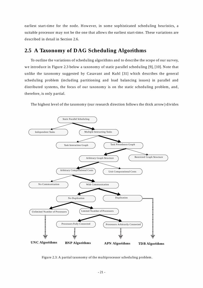
- 21 -

earliest start-time for the node. However, in some sophisticated scheduling heuristics, a

suitable processor may not be the one that allows the earliest start-time. These variations are

described in detail in Section 2.6.

2.5 A Taxonomy of DAG Scheduling Algorithms

To outline the variations of scheduling algorithms and to describe the scope of our survey,

we introduce in Figure 2.3 below a taxonomy of static parallel scheduling [9], [10]. Note that

unlike the taxonomy suggested by Casavant and Kuhl [31] which describes the general

scheduling problem (including partitioning and load balancing issues) in parallel and

distributed systems, the focus of our taxonomy is on the static scheduling problem, and,

therefore, is only partial.

The highest level of the taxonomy (our research direction follows the thick arrow) divides

Static Parallel Scheduling

Task Interaction Graph Task Precedence Graph

Figure 2.3: A partial taxonomy of the multiprocessor scheduling problem.

DuplicationNo Duplication

Limited Number of ProcessorsUnlimited Number of Processors

Processors Arbitrarily ConnectedProcessors Fully Connected

Arbitrary Computational Costs Unit Computational Costs

Arbitrary Graph Structure Restricted Graph Structure

Independent Tasks Multiple Interacting Tasks

No Communication With Communication

BNP AlgorithmsUNC Algorithms APN Algorithms TDB Algorithms

- 22 -

the scheduling problem into two categories, depending upon whether the tasks are

independent or not. Independent tasks do not have precedence relationships among each

other and hence, can be scheduled to start execution simultaneously [60], [70]. We do not deal

with the first category and, therefore, do not discuss it further. Earlier algorithms have made

simplifying assumptions about the task graph representing the program and the model of the

parallel processor system [40], [74]. Most of these algorithms assume the graph to be of a

special structure such as a tree, forks-join, etc. In general, however, parallel programs come in

a variety of structures and as such many recent algorithms are designed to tackle arbitrary

graphs. These algorithms can be further divided into two categories. Some algorithms

assume the computational costs of all the tasks to be uniform. Others assume the

computational costs of tasks to be arbitrary.

Some of the scheduling algorithms which consider the inter-task communication assume

the availability of unlimited number of processors, while some other algorithms assume an

limited number of processors. The former class of algorithms are called the UNC (unbounded

number of clusters) scheduling algorithms [105], [112], [114], [160], [189], [193] and the latter

the BNP (bounded number of processors) scheduling algorithms [1], [16], [106], [117], [133], [146],

[148], [173]. In both classes of algorithms, the processors are assumed to be fully-connected

and no attention is paid to link contention or routing strategies used for communication. The

technique employed by the UNC algorithms is also called clustering [105], [125], [146], [160],

[193]. At the beginning of the scheduling process, each node is considered a cluster. In the

subsequent steps, two clusters are merged if the merging reduces the completion time. This

merging procedure continues until no cluster can be merged. The rationale behind the UNC

algorithms is that they can take advantage of using more processors to further reduce the

schedule length. However, the clusters generated by the UNC need a postprocessing step for

mapping the clusters onto the processors because the number of processors available may be

less than the number of clusters. As a result, the final solution quality also highly depends on

the cluster-mapping step. On the other hand, the BNP algorithms do not need such

postprocessing step. It is an open question as to which of UNC and BNP is better.

We use the term cluster and processor interchangeably since in the UNC scheduling

algorithms, merging a single node cluster to another cluster is analogous to scheduling a

node to a processor.

There have been a few algorithms designed with the most general model in that the

system is assumed to consist of an arbitrary network topology, of which the links are not

contention-free. These algorithms are called the APN (arbitrary processor network) scheduling

- 23 -

algorithms. In addition to scheduling tasks, the APN algorithms also schedule messages on

the network communication links. Scheduling of messages may be dependent on the routing

strategy used by the underlying network. To optimize schedule lengths under such

unrestricted environments makes the design of an APN scheduling algorithm intricate and

challenging.

The TDB (Task-Duplication Based) scheduling algorithms also assume the availability of

an unbounded number of processors but schedule tasks with duplication to further reduce

the schedule lengths. The rationale behind the TDB scheduling algorithms is to reduce the

communication overhead by redundantly allocating some tasks to multiple processors. In

duplication-based scheduling, different strategies can be employed to select ancestor nodes

for duplication. Some of the algorithms duplicate only the direct predecessors while others

try to duplicate all possible ancestors.

In Table 2.2 we list several well known algorithms along with some of their characteristics

in the context of the preceding discussion.

2.6 Survey of DAG Scheduling Algorithms

In this section, we briefly survey algorithms for DAG scheduling reported in the

literature. We first describe early scheduling algorithms which assume a restricted DAG

model, and then proceed to describe a number of such algorithms before proceeding to

algorithms which remove all such simplifying assumptions. Throughout the discussion,

examples are used to illustrate the functionality and features of different algorithms. In

addition, the performance of the algorithms on some primitive graph structures are also

discussed. Analytical performance bounds reported in the literature are also surveyed where

appropriate. We first discuss the UNC class of algorithms, followed by BNP algorithms and

TDB algorithms. Next we describe a few of the relatively unexplored APN class of DAG

scheduling algorithms. Finally we discuss the issues of scheduling in heterogeneous

environments and the mapping problem.

2.6.1 Scheduling DAGs with Restricted Structures

Early scheduling algorithms were typically designed with simplifying assumptions about

the DAG and processor network model [1], [30], [61], [62]. For instance, the nodes in the DAG

were assumed to be of unit computation and communication was not considered; that is,

and . Furthermore, some algorithms were designed for specially

structured DAGs such as a free-tree [40], [90].

w ni( ) 1 i∀,= c ni nj,( ) 0=

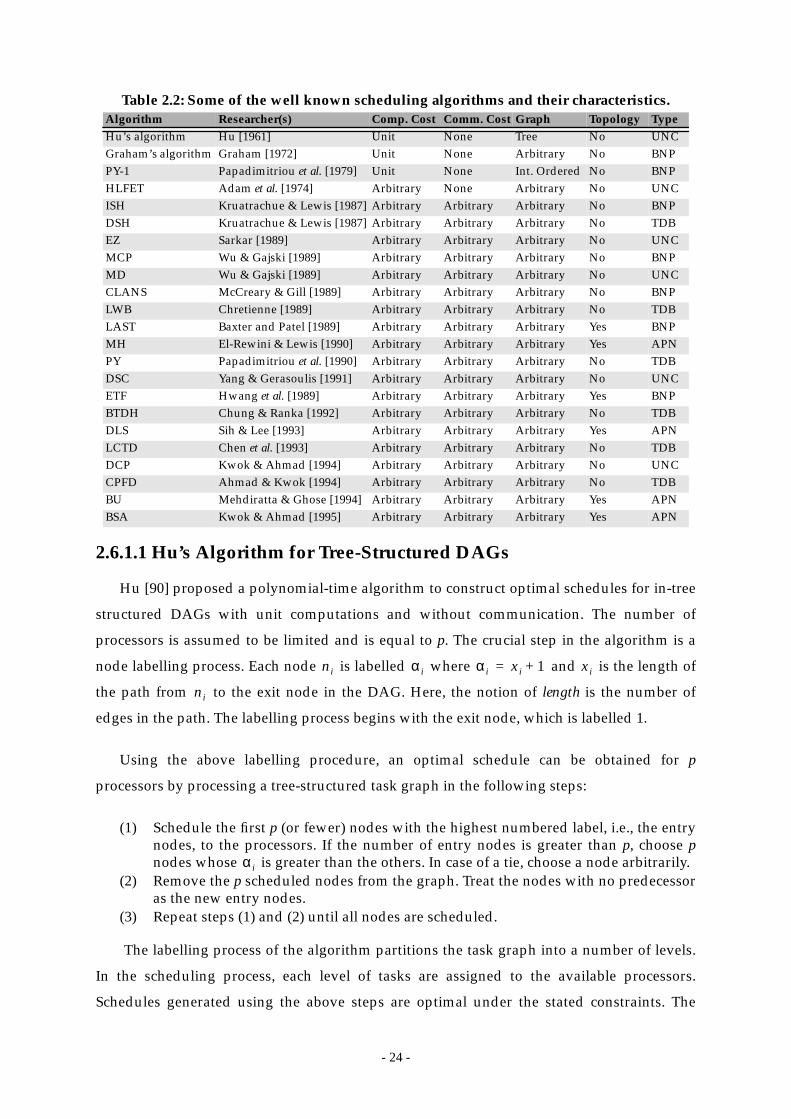
- 24 -

Table 2.2: Some of the well known scheduling algorithms and their characteristics.

2.6.1.1 Hu’s Algorithm for Tree-Structured DAGs

Hu [90] proposed a polynomial-time algorithm to construct optimal schedules for in-tree

structured DAGs with unit computations and without communication. The number of

processors is assumed to be limited and is equal to p. The crucial step in the algorithm is a

node labelling process. Each node is labelled where and is the length of

the path from to the exit node in the DAG. Here, the notion of length is the number of

edges in the path. The labelling process begins with the exit node, which is labelled 1.

Using the above labelling procedure, an optimal schedule can be obtained for p

processors by processing a tree-structured task graph in the following steps:

(1) Schedule the first p (or fewer) nodes with the highest numbered label, i.e., the entrynodes, to the processors. If the number of entry nodes is greater than p, choose pnodes whose is greater than the others. In case of a tie, choose a node arbitrarily.

(2) Remove the p scheduled nodes from the graph. Treat the nodes with no predecessoras the new entry nodes.

(3) Repeat steps (1) and (2) until all nodes are scheduled.

The labelling process of the algorithm partitions the task graph into a number of levels.

In the scheduling process, each level of tasks are assigned to the available processors.

Schedules generated using the above steps are optimal under the stated constraints. The

Algorithm Researcher(s) Comp. Cost Comm. Cost Graph Topology TypeHu’s algorithm Hu [1961] Unit None Tree No UNCGraham’s algorithm Graham [1972] Unit None Arbitrary No BNPPY-1 Papadimitriou et al. [1979] Unit None Int. Ordered No BNPHLFET Adam et al. [1974] Arbitrary None Arbitrary No UNCISH Kruatrachue & Lewis [1987] Arbitrary Arbitrary Arbitrary No BNPDSH Kruatrachue & Lewis [1987] Arbitrary Arbitrary Arbitrary No TDBEZ Sarkar [1989] Arbitrary Arbitrary Arbitrary No UNCMCP Wu & Gajski [1989] Arbitrary Arbitrary Arbitrary No BNPMD Wu & Gajski [1989] Arbitrary Arbitrary Arbitrary No UNCCLANS McCreary & Gill [1989] Arbitrary Arbitrary Arbitrary No BNPLWB Chretienne [1989] Arbitrary Arbitrary Arbitrary No TDBLAST Baxter and Patel [1989] Arbitrary Arbitrary Arbitrary Yes BNPMH El-Rewini & Lewis [1990] Arbitrary Arbitrary Arbitrary Yes APNPY Papadimitriou et al. [1990] Arbitrary Arbitrary Arbitrary No TDBDSC Yang & Gerasoulis [1991] Arbitrary Arbitrary Arbitrary No UNCETF Hwang et al. [1989] Arbitrary Arbitrary Arbitrary Yes BNPBTDH Chung & Ranka [1992] Arbitrary Arbitrary Arbitrary No TDBDLS Sih & Lee [1993] Arbitrary Arbitrary Arbitrary Yes APNLCTD Chen et al. [1993] Arbitrary Arbitrary Arbitrary No TDBDCP Kwok & Ahmad [1994] Arbitrary Arbitrary Arbitrary No UNCCPFD Ahmad & Kwok [1994] Arbitrary Arbitrary Arbitrary No TDBBU Mehdiratta & Ghose [1994] Arbitrary Arbitrary Arbitrary Yes APNBSA Kwok & Ahmad [1995] Arbitrary Arbitrary Arbitrary Yes APN

ni αi αi xi 1+= xi

ni

αi

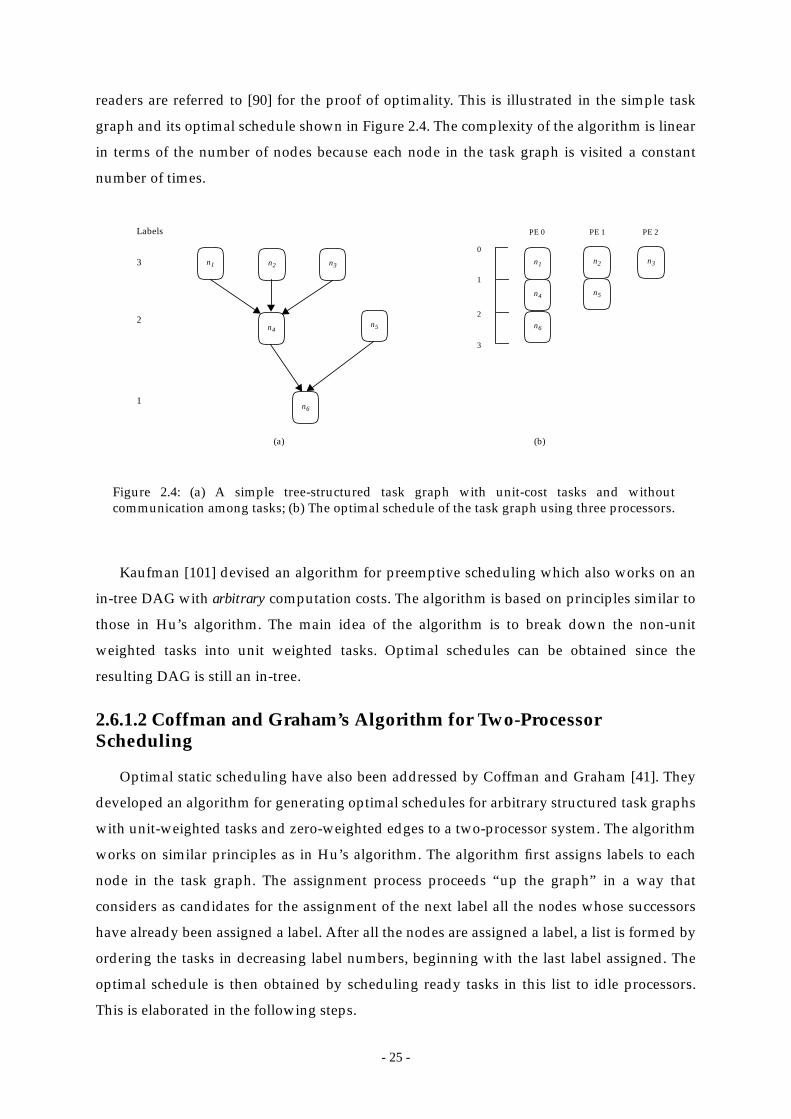
- 25 -

readers are referred to [90] for the proof of optimality. This is illustrated in the simple task

graph and its optimal schedule shown in Figure 2.4. The complexity of the algorithm is linear

in terms of the number of nodes because each node in the task graph is visited a constant

number of times.

Kaufman [101] devised an algorithm for preemptive scheduling which also works on an

in-tree DAG with arbitrary computation costs. The algorithm is based on principles similar to

those in Hu’s algorithm. The main idea of the algorithm is to break down the non-unit

weighted tasks into unit weighted tasks. Optimal schedules can be obtained since the

resulting DAG is still an in-tree.

2.6.1.2 Coffman and Graham’s Algorithm for Two-ProcessorScheduling

Optimal static scheduling have also been addressed by Coffman and Graham [41]. They

developed an algorithm for generating optimal schedules for arbitrary structured task graphs

with unit-weighted tasks and zero-weighted edges to a two-processor system. The algorithm

works on similar principles as in Hu’s algorithm. The algorithm first assigns labels to each

node in the task graph. The assignment process proceeds “up the graph” in a way that

considers as candidates for the assignment of the next label all the nodes whose successors

have already been assigned a label. After all the nodes are assigned a label, a list is formed by

ordering the tasks in decreasing label numbers, beginning with the last label assigned. The

optimal schedule is then obtained by scheduling ready tasks in this list to idle processors.

This is elaborated in the following steps.

n1

n4

n2

n6

n5

n3

Labels

3

2

1

n1 n3n2

n4 n5

n6

0

1

2

3

PE 0 PE 1 PE 2

(a) (b)

Figure 2.4: (a) A simple tree-structured task graph with unit-cost tasks and withoutcommunication among tasks; (b) The optimal schedule of the task graph using three processors.

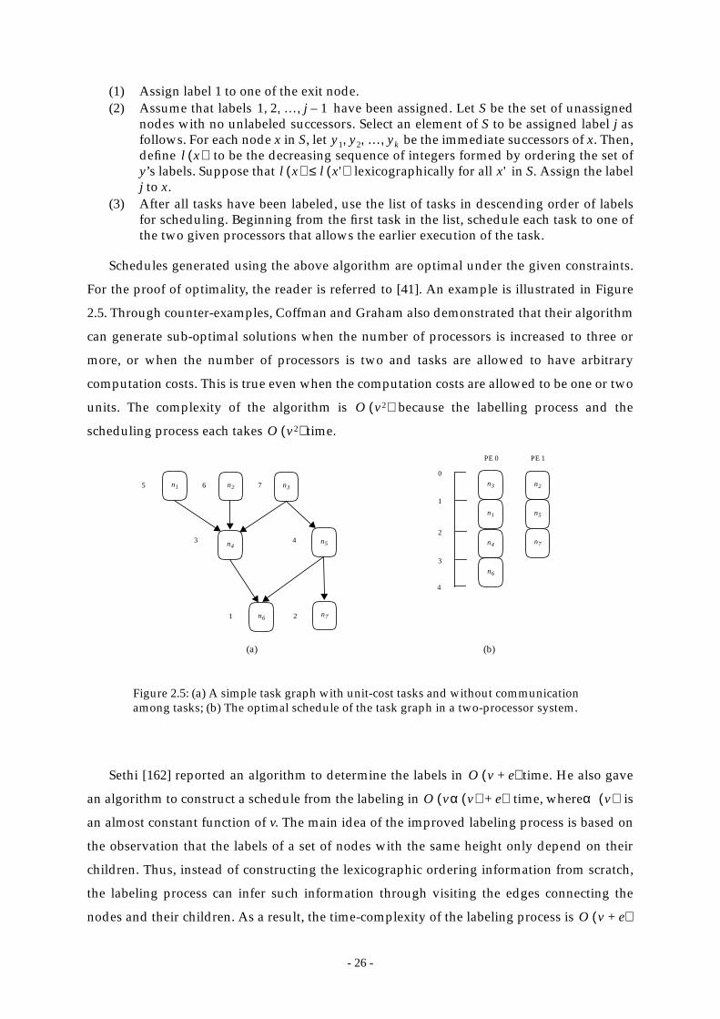
- 26 -

(1) Assign label 1 to one of the exit node.(2) Assume that labels have been assigned. Let S be the set of unassigned

nodes with no unlabeled successors. Select an element of S to be assigned label j asfollows. For each node x in S, let be the immediate successors of x. Then,define to be the decreasing sequence of integers formed by ordering the set ofy’s labels. Suppose that lexicographically for all in S. Assign the labelj to x.

(3) After all tasks have been labeled, use the list of tasks in descending order of labelsfor scheduling. Beginning from the first task in the list, schedule each task to one ofthe two given processors that allows the earlier execution of the task.

Schedules generated using the above algorithm are optimal under the given constraints.

For the proof of optimality, the reader is referred to [41]. An example is illustrated in Figure

2.5. Through counter-examples, Coffman and Graham also demonstrated that their algorithm

can generate sub-optimal solutions when the number of processors is increased to three or

more, or when the number of processors is two and tasks are allowed to have arbitrary

computation costs. This is true even when the computation costs are allowed to be one or two

units. The complexity of the algorithm is because the labelling process and the

scheduling process each takes time.

Sethi [162] reported an algorithm to determine the labels in time. He also gave

an algorithm to construct a schedule from the labeling in time, where is

an almost constant function of v. The main idea of the improved labeling process is based on

the observation that the labels of a set of nodes with the same height only depend on their

children. Thus, instead of constructing the lexicographic ordering information from scratch,

the labeling process can infer such information through visiting the edges connecting the

nodes and their children. As a result, the time-complexity of the labeling process is

1 2 … j 1–, , ,

y1 y2 … yk, , ,l x( )

l x( ) l x'( )≤ x'

O v2( )

n1

n4

n2

n6

n5

n3

n71 2

43

5 6 7 n3 n2

n1 n5

n4 n7

n6

0

1

2

3

4

PE 0 PE 1

(a) (b)

Figure 2.5: (a) A simple task graph with unit-cost tasks and without communicationamong tasks; (b) The optimal schedule of the task graph in a two-processor system.

O v2( )

O v e+( )

O vα v( ) e+( ) α v( )

O v e+( )

- 27 -

instead of . The construction of the final schedule is done with the aid of a set data

structure, for which v access operations can be performed in , where is the

inverse Ackermann’s function. Details of Sethi’s algorithms can be found in [162].

2.6.1.3 Scheduling Interval-Ordered DAGs

Papadimitriou and Yannakakis [151] investigated the problem of scheduling unit-

computational interval-ordered tasks to multiprocessors. In an interval-ordered DAG, two

nodes are precedence-related if and only if the nodes can be mapped to non-overlapping

intervals on the real line [57]. An example of an interval-ordered DAG is shown in Figure 2.6.

Based on the interval-ordered property, the number of successors of a node can be used as a

priority to construct a list. An optimal list schedule can be constructed in time.

However, as mentioned earlier, the problem becomes NP-complete if the DAG is allowed to

have arbitrary computation costs. Ali and El-Rewini [11] worked on the problem of

scheduling interval-ordered DAGs with unit computation costs and unit communication

costs. They showed that the problem is tractable and devised an algorithm to generate

optimal schedules. In their algorithm, which is similar to that of Papadimitriou and

Yannakakis, the number of successors is used as a node priority for scheduling.

2.6.2 Scheduling Arbitrary DAGs without Communication

In this section, we discuss algorithms for scheduling arbitrary structured DAGs in which

computation costs are arbitrary but communication costs are zero.

2.6.2.1 Level-based Heuristics

Adam et al. [1] performed an extensive simulation study of the performance of a number

O v2( )

O vα v( )( ) α v( )

n1

n4

n2

n6

n5

n3

n7

Interval 1

Interval 2

Interval 3

Figure 2.6: (a) A unit-computational interval ordered DAG. (b) An optimal schedule of the DAG.

n3 n2

n1 n5

n4 n7

n6

0

1

2

3

4

PE 0 PE 1

(a) (b)

O v e+( )

O ve( )

- 28 -

of level-based list scheduling heuristics. The heuristics examined are:

• HLFET (Highest Level First with Estimated Times): The notion of level is the sum of

computation costs of all the nodes along the longest path from the node to an exit node.

• HLFNET (Highest Levels First with No Estimated Times): In this heuristic, all nodes are

scheduled as if they were of unit cost.

• Random: The nodes in the DAG are assigned priorities randomly.

• SCFET (Smallest Co-levels First with Estimated Times): A co-level of a node is

determined by computing the sum of the longest path from an entry node to the node.

A node has a higher priority if it has the smaller co-level.

• SCFNET (Smallest Co-levels First with No Estimated Times): This heuristic is the same

as SCFET except that it schedules the nodes as if they were of unit costs.

In [1], an extensive simulation study was conducted using randomly generated DAGs.

The performance of the heuristics were ranked in the following order: HLFET, HLFNET,

SCFNET, Random, and SCFET. The study provided strong evidence that the CP (critical path)

based algorithms have near-optimal performance. In another study conducted by Kohler

[104], the performance of the CP-based algorithms improved as the number of processors

increased.

Kasahara et al. [100] proposed an algorithm called CP/MISF (critical path/ most

immediate successors first), which is a variation of the HLFET algorithm. The major

improvement of CP/MISF over HLFET is that when assigning priorities, ties are broken by

selecting the node with a larger number of immediate successors.

In a recent study, Shirazi et al. [165] proposed two algorithms for scheduling DAGs to

multiprocessors without communication. The first algorithm, called HNF (Heavy Node

First), is based on a simple local analysis of the DAG nodes at each level. The second

algorithm, WL (Weighted Length), considers a global view of a DAG by taking into account

the relationship among the nodes at different levels. Compared to a critical-path-based

algorithm, Shirazi et al. showed that the HNF algorithm is more preferable for its low

complexity and good performance.

2.6.2.2 A Branch-and-Bound Approach

In addition to CP/MISF, Kasahara et al. [100] also reported an scheduling algorithm based

on a branch-and-bound approach. Using Kohler’s [103] general representation for branch-

- 29 -

and-bound algorithms, Kasahara et al. devised a depth-first search procedure to construct

near-optimal schedules. Prior to the depth-first search process, priorities are assigned to those

nodes in the DAG which may be generated during the search process. The priorities are

determined using the priority list of the CP/MISF method. In this way the search procedure

can be more efficient both in terms of computing time and memory requirement. Since the

search technique is augmented by a heuristic priority assignment method, the algorithm is

called DF/IHS (depth-first with implicit heuristic search). The DF/IHS algorithm was shown

to give near optimal performance.

2.6.2.3 Analytical Performance Bounds for Scheduling withoutCommunication

Graham [77] proposed a bound on the schedule length obtained by general list

scheduling methods. Using a level-based method for generating a list for scheduling, the

schedule length SL and the optimal schedule length are related by the following:

Rammamoorthy, Chandy, and Gonzalez [156] used the concept of precedence partitions

to generate bounds on the schedule length and the number of processors for DAGs with unit

computation costs. An earliest precedence partition is a set of nodes that can be started in

parallel at the same earliest possible time constrained by the precedence relations. A latest

precedence partition is a set of nodes which must be executed at the same latest possible time

constrained by the precedence relations. For any i and j, and . The

precedence partitions group tasks into subsets to indicate the earliest and latest times during

which tasks can be started and still guarantee minimum execution time for the graph. This

time is given by the number of partitions and is a measure of the longest path in the graph.

For a graph of l levels, the minimum execution time is l units. In order to execute a graph in

the minimum time, the absolute minimum number of processors required is given by

.

Rammamoorthy et al. [156] also developed algorithms to determine the minimum

number of processors required to process a graph in the least possible amount of time, and to

determine the minimum time necessary to process a task graph given k processors. Since a

dynamic programming approach is employed, the computational time required to obtain the

optimal solution is quite considerable.

Fernandez et al. [55] devised improved bounds on the minimum number of processors

SLopt

SL 2 1p---–

SLopt.≤

Ei

Ei Ej φ=∩ Li Lj∩ φ=

max1 i l≤ ≤ Ei Li∩{ }

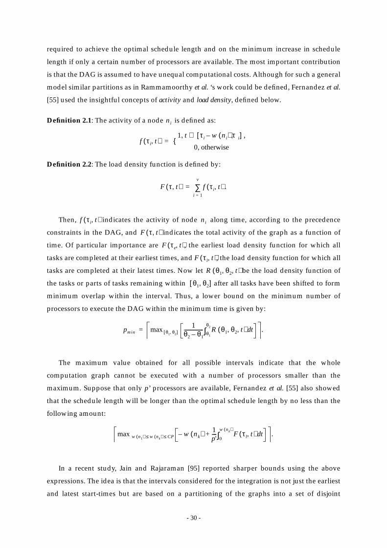
- 30 -

required to achieve the optimal schedule length and on the minimum increase in schedule

length if only a certain number of processors are available. The most important contribution

is that the DAG is assumed to have unequal computational costs. Although for such a general

model similar partitions as in Rammamoorthy et al. ‘s work could be defined, Fernandez et al.

[55] used the insightful concepts of activity and load density, defined below.

Definition 2.1: The activity of a node is defined as:

Definition 2.2: The load density function is defined by:

Then, indicates the activity of node along time, according to the precedence

constraints in the DAG, and indicates the total activity of the graph as a function of

time. Of particular importance are , the earliest load density function for which all

tasks are completed at their earliest times, and , the load density function for which all

tasks are completed at their latest times. Now let be the load density function of

the tasks or parts of tasks remaining within after all tasks have been shifted to form

minimum overlap within the interval. Thus, a lower bound on the minimum number of

processors to execute the DAG within the minimum time is given by:

The maximum value obtained for all possible intervals indicate that the whole

computation graph cannot be executed with a number of processors smaller than the

maximum. Suppose that only p’ processors are available, Fernandez et al. [55] also showed

that the schedule length will be longer than the optimal schedule length by no less than the

following amount:

In a recent study, Jain and Rajaraman [95] reported sharper bounds using the above

expressions. The idea is that the intervals considered for the integration is not just the earliest

and latest start-times but are based on a partitioning of the graphs into a set of disjoint

ni

f τi t,( )1 t τi w ni( ) τi,–[ ] ,∈,

0 otherwise,{=

F τ t,( ) f τi t,( ) .i 1=

v

∑=

f τi t,( ) ni

F τ t,( )

F τe t,( )

F τl t,( )

R θ1 θ2 t, ,( )

θ1 θ2,[ ]

pmin max θ1 θ2,[ ]1

θ2 θ1–---------------- R θ1 θ2 t, ,( ) td

θ1

θ2

∫ .=

max w n1( ) w nk( ) CP≤≤ w nk( )–1p'---- F τl t,( ) td

0

w nk( )∫+ .

- 31 -

sections. They also devised an upper bound on the schedule length, which is useful in

determining the worst case behavior of a DAG. Not only are their new bounds easier to

compute but are also tighter in that the DAG partitioning strategy enhances the accuracy of

the load activity function.

2.6.3 UNC Scheduling

In this section we survey the UNC class of scheduling algorithms. In particular, we will

describe in more details five UNC scheduling algorithms: the EZ, LC, DSC, MD, and DCP

algorithms. The DAG shown in Figure 2.2 is used to illustrate the scheduling process of these

algorithms. In order to examine the approximate optimality of the algorithms, we will first

describe the scheduling of two primitive DAG structures: the fork set and the join set. Some

work on theoretical performance analysis of UNC scheduling is also discussed in the last

subsection.

2.6.3.1 Scheduling of Primitive Graph Structures

To highlight the different characteristics of the algorithms described below, it is useful to

consider how the algorithms work on some primitive graph structures. Two commonly used

primitive graph structures are fork and join [66], examples of which are shown in Figure 2.7.

In the following, we derive the optimal schedule lengths for these primitive structures. The

optimal schedule lengths can then be used as a basis for comparing the functionality of the

scheduling algorithms described later in this section.

Without loss of generality, assume that for the fork structure, we have:

n1 n2nk

n3

nx

Figure 2.7: (a) A fork set; and (b) a join set.

c(n1, nx)

n1 n2nk

n3

nx

(a) (b)

c(n2, nx) c(n3, nx)c(nk, nx)

c(nx, n1)

c(nx, n2)c(nx, n3)

c(nx, nk)

c nx n1,( ) w n1( ) c nx n2,( ) w n2( ) … c nx nk,( ) w nk( ) .+≥ ≥+≥+

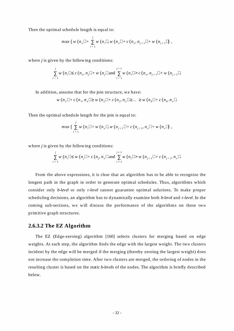
- 32 -

Then the optimal schedule length is equal to:

where j is given by the following conditions:

In addition, assume that for the join structure, we have:

Then the optimal schedule length for the join is equal to:

where j is given by the following conditions:

From the above expressions, it is clear that an algorithm has to be able to recognize the

longest path in the graph in order to generate optimal schedules. Thus, algorithms which

consider only b-level or only t-level cannot guarantee optimal solutions. To make proper

scheduling decisions, an algorithm has to dynamically examine both b-level and t-level. In the

coming sub-sections, we will discuss the performance of the algorithms on these two

primitive graph structures.

2.6.3.2 The EZ Algorithm

The EZ (Edge-zeroing) algorithm [160] selects clusters for merging based on edge

weights. At each step, the algorithm finds the edge with the largest weight. The two clusters

incident by the edge will be merged if the merging (thereby zeroing the largest weight) does

not increase the completion time. After two clusters are merged, the ordering of nodes in the

resulting cluster is based on the static b-levels of the nodes. The algorithm is briefly described

below.

max w nx( ) w ni( ) w nx( ) c nx nj 1+,( ) w nj 1+( )+ +,i 1=

j

∑+{ } ,

w ni( ) c nx nj,( ) w nj( ) and w ni( ) c nx nj 1+,( ) w nj 1+( ) .+>i 1=

j 1+

∑+≤i 1=

j

∑

w n1( ) c n1 nx,( ) w n2( ) c n2 nx,( ) … w nk( ) c nk nx,( ) .+≥ ≥+≥+

max w ni( ) w nx( ) w nj 1+( ) c nj 1+ nx,( ) w nx( )+ +,+i 1=

j

∑{ } ,

w ni( ) w nj( ) c nj nx,( ) and w ni( ) w nj 1+( ) c nj 1+ nx,( ) .+>i 1=

j 1+

∑+≤i 1=

j

∑

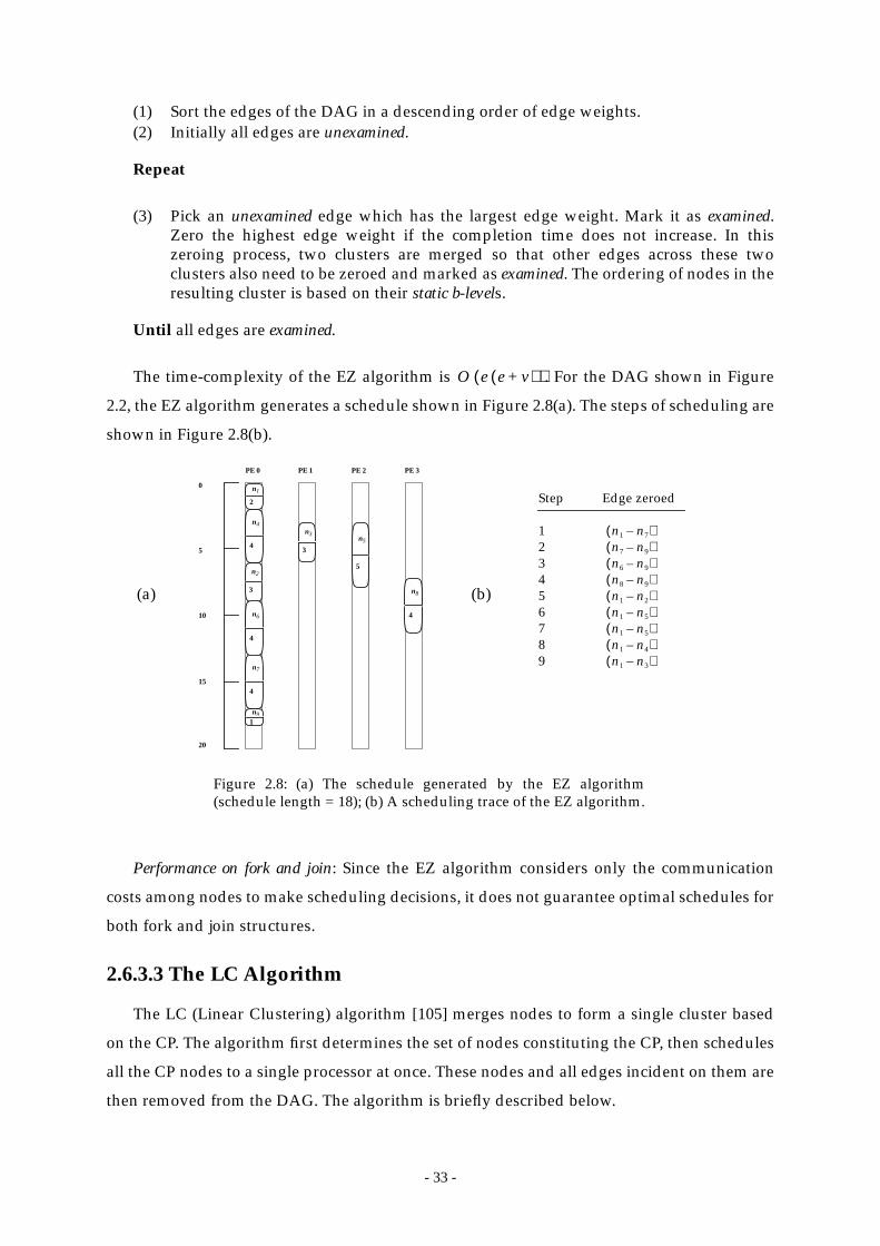
- 33 -

(1) Sort the edges of the DAG in a descending order of edge weights.(2) Initially all edges are unexamined.

Repeat

(3) Pick an unexamined edge which has the largest edge weight. Mark it as examined.Zero the highest edge weight if the completion time does not increase. In thiszeroing process, two clusters are merged so that other edges across these twoclusters also need to be zeroed and marked as examined. The ordering of nodes in theresulting cluster is based on their static b-levels.

Until all edges are examined.

The time-complexity of the EZ algorithm is . For the DAG shown in Figure

2.2, the EZ algorithm generates a schedule shown in Figure 2.8(a). The steps of scheduling are

shown in Figure 2.8(b).

Performance on fork and join: Since the EZ algorithm considers only the communication

costs among nodes to make scheduling decisions, it does not guarantee optimal schedules for

both fork and join structures.

2.6.3.3 The LC Algorithm

The LC (Linear Clustering) algorithm [105] merges nodes to form a single cluster based

on the CP. The algorithm first determines the set of nodes constituting the CP, then schedules

all the CP nodes to a single processor at once. These nodes and all edges incident on them are

then removed from the DAG. The algorithm is briefly described below.

O e e v+( )( )

PE 0 PE 1 PE 2 PE 3

Step Edge zeroed

123456789

n1 n7–( )n7 n9–( )n6 n9–( )n8 n9–( )n1 n2–( )n1 n5–( )n1 n5–( )n1 n4–( )n1 n3–( )

n1

2

n2

3

n5

5

n91

n3

3

n7

4

n4

4

0

5

10

15

20

n8

4n6

4

Figure 2.8: (a) The schedule generated by the EZ algorithm(schedule length = 18); (b) A scheduling trace of the EZ algorithm.

(a) (b)

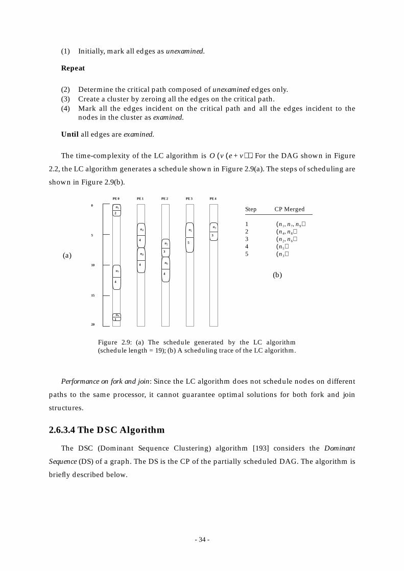
- 34 -

(1) Initially, mark all edges as unexamined.

Repeat

(2) Determine the critical path composed of unexamined edges only.(3) Create a cluster by zeroing all the edges on the critical path.(4) Mark all the edges incident on the critical path and all the edges incident to the

nodes in the cluster as examined.

Until all edges are examined.

The time-complexity of the LC algorithm is . For the DAG shown in Figure

2.2, the LC algorithm generates a schedule shown in Figure 2.9(a). The steps of scheduling are

shown in Figure 2.9(b).

Performance on fork and join: Since the LC algorithm does not schedule nodes on different

paths to the same processor, it cannot guarantee optimal solutions for both fork and join

structures.

2.6.3.4 The DSC Algorithm

The DSC (Dominant Sequence Clustering) algorithm [193] considers the Dominant

Sequence (DS) of a graph. The DS is the CP of the partially scheduled DAG. The algorithm is

briefly described below.

O v e v+( )( )

PE 0 PE 1 PE 2 PE 3

n1

2

n2

3

n5

5

n91

n3

3

n7

4

n4

4

0

5

10

15

20

n8

4 n6

4

Figure 2.9: (a) The schedule generated by the LC algorithm(schedule length = 19); (b) A scheduling trace of the LC algorithm.

Step CP Merged

12345

n1 n7 n9, ,( )n4 n8,( )n2 n6,( )n5( )n3( )

PE 4

(a)

(b)

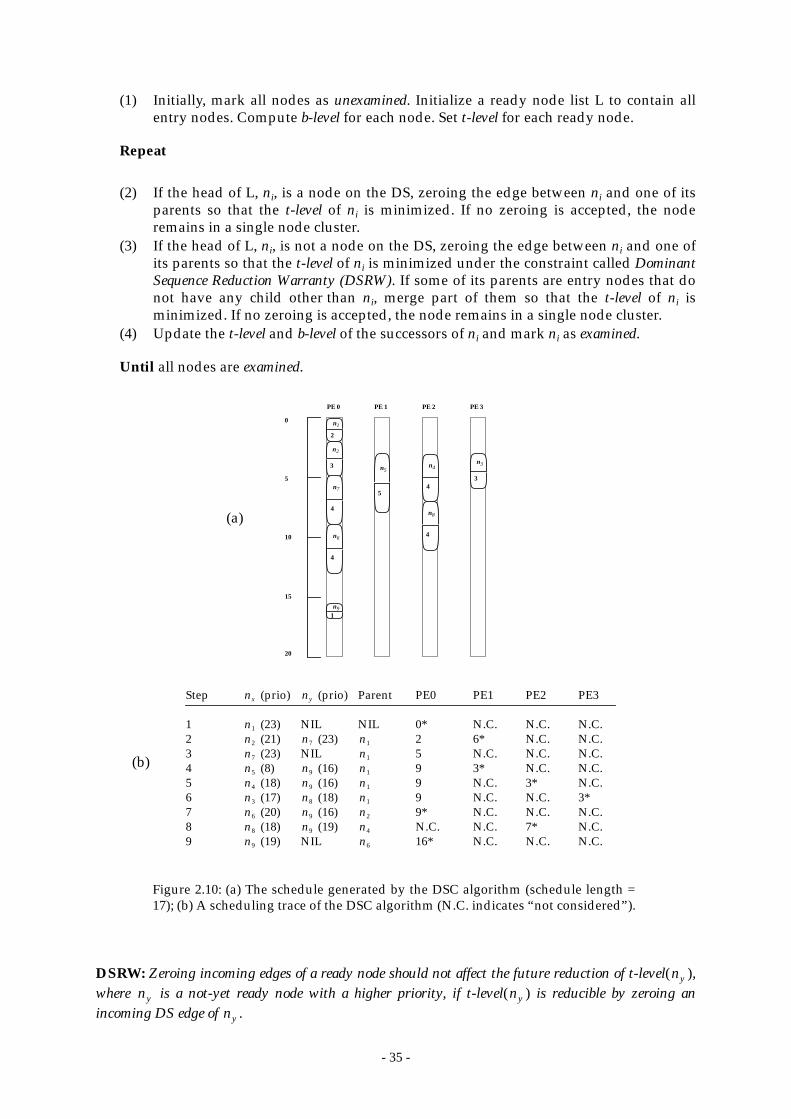
- 35 -

(1) Initially, mark all nodes as unexamined. Initialize a ready node list L to contain allentry nodes. Compute b-level for each node. Set t-level for each ready node.

Repeat

(2) If the head of L, ni, is a node on the DS, zeroing the edge between ni and one of itsparents so that the t-level of ni is minimized. If no zeroing is accepted, the noderemains in a single node cluster.

(3) If the head of L, ni, is not a node on the DS, zeroing the edge between ni and one ofits parents so that the t-level of ni is minimized under the constraint called DominantSequence Reduction Warranty (DSRW). If some of its parents are entry nodes that donot have any child other than ni, merge part of them so that the t-level of ni isminimized. If no zeroing is accepted, the node remains in a single node cluster.

(4) Update the t-level and b-level of the successors of ni and mark ni as examined.

Until all nodes are examined.

DSRW: Zeroing incoming edges of a ready node should not affect the future reduction of t-level( ),where is a not-yet ready node with a higher priority, if t-level( ) is reducible by zeroing anincoming DS edge of .

PE 0 PE 1 PE 2 PE 3

Step (prio) (prio) Parent PE0 PE1 PE2 PE3

1 (23) NIL NIL 0* N.C. N.C. N.C.2 (21) (23) 2 6* N.C. N.C.3 (23) NIL 5 N.C. N.C. N.C.4 (8) (16) 9 3* N.C. N.C.5 (18) (16) 9 N.C. 3* N.C.6 (17) (18) 9 N.C. N.C. 3*7 (20) (16) 9* N.C. N.C. N.C.8 (18) (19) N.C. N.C. 7* N.C.9 (19) NIL 16* N.C. N.C. N.C.

nx ny

n1

n2 n7 n1

n7 n1

n5 n9 n1

n4 n9 n1

n3 n8 n1

n6 n9 n2

n8 n9 n4

n9 n6

n1

2

n2

3 n5

5

n91

n3

3n7

4

n4

4

0

5

10

15

20

n8

4n6

4

Figure 2.10: (a) The schedule generated by the DSC algorithm (schedule length =17); (b) A scheduling trace of the DSC algorithm (N.C. indicates “not considered”).

(a)

(b)

ny

ny ny

ny

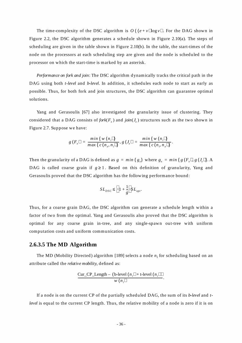
- 36 -

The time-complexity of the DSC algorithm is . For the DAG shown in

Figure 2.2, the DSC algorithm generates a schedule shown in Figure 2.10(a). The steps of

scheduling are given in the table shown in Figure 2.10(b). In the table, the start-times of the

node on the processors at each scheduling step are given and the node is scheduled to the

processor on which the start-time is marked by an asterisk.

Performance on fork and join: The DSC algorithm dynamically tracks the critical path in the

DAG using both t-level and b-level. In addition, it schedules each node to start as early as

possible. Thus, for both fork and join structures, the DSC algorithm can guarantee optimal

solutions.

Yang and Gerasoulis [67] also investigated the granularity issue of clustering. They

considered that a DAG consists of fork( ) and join( ) structures such as the two shown in

Figure 2.7. Suppose we have:

Then the granularity of a DAG is defined as where . A

DAG is called coarse grain if . Based on this definition of granularity, Yang and

Gerasoulis proved that the DSC algorithm has the following performance bound:

Thus, for a coarse grain DAG, the DSC algorithm can generate a schedule length within a

factor of two from the optimal. Yang and Gerasoulis also proved that the DSC algorithm is

optimal for any coarse grain in-tree, and any single-spawn out-tree with uniform

computation costs and uniform communication costs.

2.6.3.5 The MD Algorithm

The MD (Mobility Directed) algorithm [189] selects a node ni for scheduling based on an

attribute called the relative mobility, defined as:

If a node is on the current CP of the partially scheduled DAG, the sum of its b-level and t-

level is equal to the current CP length. Thus, the relative mobility of a node is zero if it is on

O e v+( ) vlog( )

Fx Jx

g Fx( )min w ni( ){ }

max c nx ni,( ){ }------------------------------------------ g Jx( ),min w ni( ){ }

max c ni nx,( ){ }------------------------------------------ .= =

g min gx{ }= gx min g Fx( ) g Jx( ),{ }=

g 1≥

SLDSC 1 1g---+

SLopt.≤

Cur_CP_Length b-levelni( ) t-level ni( )+( )–w ni( )------------------------------------------------------------------------------------------------------------------.

- 37 -

the current CP. The algorithm is described below.

(1) Mark all nodes as unexamined. Initially, there is no cluster.

Repeat

(2) Compute the relative mobility for each node.(3) Let L' be the group of unexamined nodes with the minimum relative mobility. Let ni

be a node in L' that does not have any predecessors in L'. Start from the first cluster,check whether there is any cluster that can accommodate ni. In the checking process,all idle time slots in a cluster are examined until one is found to be large enough tohold ni. A large enough idle time slot may be created by pulling already schedulednodes downward because the start-times of the already scheduled nodes are notfixed yet. If ni cannot be scheduled to the first cluster, try the second cluster, and soon. If ni cannot be scheduled to any existing cluster, leave it as a new cluster.

(4) When ni is scheduled to cluster m, all edges connecting ni and other nodes alreadyscheduled to cluster m are changed to zero. If ni is scheduled before node nj oncluster m, add an edge with weight zero from ni to nj in the DAG. If ni is scheduledafter node nj on the cluster, add an edge with weight zero from nj to ni, then check ifthe adding edges form a loop. If so, schedule ni to the next available space.

(5) Mark ni as examined.

Until all nodes are examined.

The time-complexity of the MD algorithm is . For the DAG shown in Figure 2.2, the

MD algorithm generates a schedule shown in Figure 2.11(a). The steps of scheduling are

given in the table shown in Figure 2.11(b). In the table, the start-times of the node on the

processors at each scheduling step are given and the node is scheduled to the processor on

which the start-time is marked by an asterisk.

Performance on fork and join: Using the notion of relative mobility, the MD algorithm is also

able to track the critical path of the DAG in the scheduling process. Thus, the algorithm can

generate optimal schedules for fork and join as well.

2.6.3.6 The DCP Algorithm

The DCP (Dynamic Critical Path) algorithm [111], [112], [114] is proposed by Kwok and

Ahmad and is designed based on an attribute which is slightly different from the relative

mobility used in the MD algorithm. Essentially, the DCP algorithm examines a node ni for

scheduling if, among all nodes, ni has the smallest difference between its ALST (Absolute-

Latest-Start-Time) and AEST (Absolute-Earliest-Start-Time). The value of such difference is

equivalent to the value of the node’s mobility, defined as:

. The DCP algorithm uses a lookahead strategy

to find a better cluster for a given node. The DCP algorithm is briefly described below.

O v3( )

Cur_CP_Length b-levelni( ) t-level ni( )+( )–( )

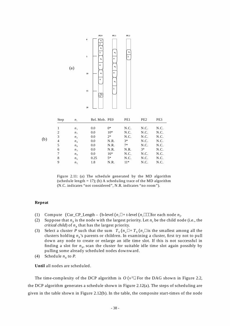
- 38 -

Repeat

(1) Compute for each node ni.(2) Suppose that nx is the node with the largest priority. Let nc be the child node (i.e., the

critical child) of nx that has the largest priority.(3) Select a cluster P such that the sum is the smallest among all the

clusters holding nx’s parents or children. In examining a cluster, first try not to pulldown any node to create or enlarge an idle time slot. If this is not successful infinding a slot for nx, scan the cluster for suitable idle time slot again possibly bypulling some already scheduled nodes downward.

(4) Schedule nx to P.

Until all nodes are scheduled.

The time-complexity of the DCP algorithm is . For the DAG shown in Figure 2.2,

the DCP algorithm generates a schedule shown in Figure 2.12(a). The steps of scheduling are

given in the table shown in Figure 2.12(b). In the table, the composite start-times of the node

PE 0 PE 1 PE 2

Step Rel. Mob. PE0 PE1 PE2 PE3

1 0.0 0* N.C. N.C. N.C.2 0.0 10* N.C. N.C. N.C.3 0.0 2* N.C. N.C. N.C.4 0.0 N.R. 3* N.C. N.C.5 0.0 N.R. 7* N.C. N.C.6 0.0 N.R. N.R. 3* N.C.7 0.0 16* N.C. N.C. N.C.8 0.25 5* N.C. N.C. N.C.9 1.8 N.R. 11* N.C. N.C.

ni

n1

n7

n2

n4

n8

n3

n9

n6

n5

n1

2

n2

3

n5

5

n91

n3

3

n7

4

n4

4

0

5

10

15

20

n8

4

n6

4

Figure 2.11: (a) The schedule generated by the MD algorithm(schedule length = 17); (b) A scheduling trace of the MD algorithm(N.C. indicates “not considered”, N.R. indicates “no room”).

(a)

(b)

Cur_CP_Length b-levelni( ) t-level ni( )+( )–( )

TS nx( ) TS nc( )+

O v3( )

- 39 -

(i.e., the start-time of the node plus that of its critical child) on the processors at each

scheduling step are given and the node is scheduled to the processor on which the start-time

is marked by an asterisk.

Performance on fork and join: Since the DCP algorithm examines the first unscheduled node

on the current critical path by using mobility measures, it constructs optimal solutions for

fork and join graph structures.

2.6.3.7 Other UNC Approaches

Kim and Yi [106] proposed a two-pass scheduling algorithm with time-complexity

. The idea of the algorithm comes from the scheduling of in-trees. Kim and Yi

observed that an in-tree can be efficiently scheduled by iteratively merging a node to the

parent node that allows the earliest completion time. To extend this idea to arbitrary

structured DAGs, Kim and Yi devised a two-pass algorithm. In the first pass, an independent

PE 0 PE 1 PE 2

Step AEST ALST Cri. Child PE0 PE1 PE2 PE3

1 0 0 0+10* N.C. N.C. N.C.2 12 12 10+19* 12+19 N.C. N.C.3 6 6 2+5* 6+9 N.C. N.C.4 3 3 N.R. 3+7* N.C. N.C.5 8 8 N.C. 7+15* 8+15 N.C.6 3 3 N.R. N.R. 3+7* N.C.7 16 16 NIL 16+0 15+0* N.C. 16+08 6 6 N.R. 11+0* N.C. 6+159 3 11 NIL 9+0 N.R. 6+0* N.C.

ni

n1 n7

n7 n9

n2 n7

n4 n8

n8 n9

n3 n8

n9

n6 n9

n5

n1

2

n2

3

n5

5

n91

n3

3n7

4

n4

4

0

5

10

15

20

n8

4

n6

4

Figure 2.12: (a) The schedule generated by the DCP algorithm(schedule length = 16); (b) A scheduling trace of the DCP algorithm(N.C. indicates “not considered”, N.R. indicates “no room”).

(a)

(b)

O v vlog( )

- 40 -

v-graph is constructed for each exit node and an iterative scheduling process is carried out on

the v-graphs. This phase is called forward-scheduling. Since some intermediate nodes may be

assigned to different processors in different schedules, a backward-scheduling phase—the

second pass of the algorithm—is needed to resolve the conflicts. In their simulation study, the

two-pass algorithm outperformed a simulated annealing approach. Moreover, as the

principles of the algorithm rooted from scheduling trees, the algorithm is optimal for both

fork and join structures.

2.6.3.8 Theoretical Analysis for UNC Scheduling

In addition to the granularity analysis performed for the DSC algorithm, Yang and

Gerasoulis [191] worked on the general analysis for UNC scheduling. They introduced a

notion called which is defined below.

Definition 2.3: Let be the optimum schedule length at step i of a UNC scheduling

algorithm. A UNC scheduling algorithm is called if where is

a given constant.

In their study, they examined two critical-path-based simple UNC scheduling heuristics

called RCP and RCP*. Essentially, both heuristics use b-level as the scheduling priority but

with a slight difference in that RCP* uses (b-level – ) as the priority. They showed that

both heuristics are , and thus, demonstrated that critical path based scheduling

algorithms are near-optimal.

2.6.4 BNP Scheduling

In this section we survey the BNP class of scheduling algorithms. In particular we discuss

in detail six BNP scheduling algorithms: the HLFET, ISH, MCP, ETF, DLS, and LAST

algorithms. Again the DAG shown in Figure 2.2 is used to illustrate the scheduling process of

these algorithms. The analytical performance bounds of BNP scheduling will also be

discussed in the last subsection.

2.6.4.1 The HLFET Algorithm

The HLFET (Highest Level First with Estimated Times) algorithm [1] is one of the

simplest list scheduling algorithms and is described below.

δ-lopt

SLilopt

δ-lopt maxi SLi SLilopt–{ } δ≤ δ

w ni( )

δ-lopt

- 41 -

(1) Calculate the static b-level (i.e., SL or static level) of each node.(2) Make a ready list in a descending order of static b-level. Initially, the ready list

contains only the entry nodes. Ties are broken randomly.

Repeat

(3) Schedule the first node in the ready list to a processor that allows the earliestexecution, using the non-insertion approach.

(4) Update the ready list by inserting the nodes that are now ready.


The time-complexity of the HLFET algorithm is . For the DAG shown in Figure 2.2,

the HLFET algorithm generates a schedule shown in Figure 2.13(a). The steps of scheduling

are given in the table shown in Figure 2.13(b). In the table, the start-times of the node on the

O v2( )

PE 0 PE 1 PE 2 PE 3

Step PE0 PE1 PE2 PE3

1 0* N.C. N.C. N.C.2 2* 3 N.C. N.C.3 6* 6 N.C. N.C.4 9 3* N.C. N.C.5 9 6 3* N.C.6 9* 10 10 107 13 12* 12 128 13 16 8 7*9 22 18* 22 22

ni

n1

n4

n2

n3

n5

n6

n7

n8

n9

n1

2

n2

3

n5

5

n91

n3

3

n7

4

n4

4

0

5

10

15

20

n8

4n6

4

Figure 2.13: (a) The schedule generated by the HLFET algorithm (schedule length =19); (b) A scheduling trace of the HLFET algorithm (N.C. indicates “not considered”).

(a)

(b)

- 42 -



Performance on fork and join: Since the HLFET algorithm schedules nodes based on b-level

only, it cannot guarantee optimal schedules for fork and join structures even if given

sufficient processors.

2.6.4.2 The ISH Algorithm

The ISH (Insertion Scheduling Heuristic) algorithm [108] uses the “scheduling holes”—

the idle time slots—in the partial schedules. The algorithm tries to fill the holes by scheduling

other nodes into them and uses static b-level as the priority of a node. The algorithm is briefly

described below.

(1) Calculate the static b-level of each node.(2) Make a ready list in a descending order of static b-level. Initially, the ready list

contains only the entry nodes. Ties are broken randomly.

Repeat

(3) Schedule the first node in the ready list to the processor that allows the earliestexecution, using the non-insertion algorithm.

(4) If scheduling of this node causes an idle time slot, then find as many nodes aspossible from the ready list that can be scheduled to the idle time slot but cannot bescheduled earlier on other processors.

(5) Update the ready list by inserting the nodes that are now ready.


The time-complexity of the ISH algorithm is . For the DAG shown in Figure 2.2, the

ISH algorithm generates a schedule shown in Figure 2.14(a). The steps of scheduling are



which the start-time is marked by an asterisk. Hole tasks are the nodes considered for

scheduling into the idle time slots.

Performance on fork and join: Since the ISH algorithm schedules nodes based on b-level only,

it cannot guarantee optimal schedules for fork and join structures even if given sufficient

processors.

2.6.4.3 The MCP Algorithm

The MCP (Modified Critical Path) algorithm [189] uses the ALAP of a node as the

O v2( )

- 43 -

scheduling priority. The MCP algorithm first computes the ALAPs of all the nodes, then

constructs a list of nodes in an ascending order of ALAP times. Ties are broken by

considering the ALAP times of the children of a node. The MCP algorithm then schedules the

nodes on the list one by one such that a node is scheduled to a processor that allows the

earliest start-time using the insertion approach. The MCP algorithm and the ISH algorithm

have different philosophies in utilizing the idle time slot: MCP looks for an idle time slot for a

given node, while ISH looks for a hole node to fit in a given idle time slot. The algorithm is

briefly described below.

PE 0 PE 1 PE 2 PE 3

Step PE0 PE1 PE2 PE3 Idle Slot Hole Tasks (start-time)

1 0* N.C. N.C. N.C. NIL NIL2 2* 3 N.C. N.C. NIL NIL3 6 3* N.C. N.C. [0..3] (6), (3)4 6 6 6* N.C. [0..6] (3), (7)5 6 6 9 3* [0..3] (10), (12), (7)6 7* 7 9 8 [6..7] (10), (10)7 11* 12 12 12 NIL NIL8 15 10 9* 10 NIL NIL9 18* 21 21 21 [15..18] NIL

ni

n1

n4

n3 n2 n5

n2 n5 n8

n5 n6 n7 n8

n8 n6 n7

n7

n6

n9

n1

2

n2

3

n5

5

n91

n3

3

n7

4

n4

4

0

5

10

15

20

n8

4

n6

4

Figure 2.14: (a) The schedule generated by the ISH algorithm (schedule length =19); (b) A scheduling trace of the ISH algorithm (N.C. indicates “not considered”).

(a)

(b)

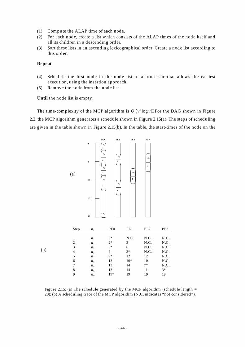
- 44 -

(1) Compute the ALAP time of each node.(2) For each node, create a list which consists of the ALAP times of the node itself and

all its children in a descending order.(3) Sort these lists in an ascending lexicographical order. Create a node list according to

this order.

Repeat

(4) Schedule the first node in the node list to a processor that allows the earliestexecution, using the insertion approach.

(5) Remove the node from the node list.

Until the node list is empty.

The time-complexity of the MCP algorithm is . For the DAG shown in Figure

2.2, the MCP algorithm generates a schedule shown in Figure 2.15(a). The steps of scheduling

are given in the table shown in Figure 2.15(b). In the table, the start-times of the node on the

O v2 vlog( )

PE 0 PE 1 PE 2 PE 3


1 0* N.C. N.C. N.C.2 2* 3 N.C. N.C.3 6* 6 N.C. N.C.4 9 3* N.C. N.C.5 9* 12 12 N.C.6 13 10* 10 N.C.7 13 14 7* N.C.8 13 14 11 3*9 19* 19 19 19

ni

n1

n4

n2

n3

n7

n6

n8

n5

n9

n1

2

n2

3

n5

5

n91

n3

3

n7

4

n4

4

0

5

10

15

20

n8

4

n6

4

Figure 2.15: (a) The schedule generated by the MCP algorithm (schedule length =20); (b) A scheduling trace of the MCP algorithm (N.C. indicates “not considered”).

(a)

(b)

- 45 -



Performance on fork and join: Since the MCP algorithm schedules nodes based on ALAP

(effectively based on b-level) only, it cannot guarantee optimal schedules for fork and join

structures even if given sufficient processors.

2.6.4.4 The ETF Algorithm

The ETF (Earliest Time First) algorithm [93] computes, at each step, the earliest start-times

for all ready nodes and then selects the one with the smallest start-time. Here, the earliest

start-time of a node is computed by examining the start-time of the node on all processors

exhaustively. When two nodes have the same value in their earliest start-times, the ETF

algorithm breaks the tie by scheduling the one with the higher static priority. The algorithm is

described below

(1) Compute the static b-level of each node.(2) Initially, the pool of ready nodes includes only the entry nodes.

Repeat

(3) Calculate the earliest start-time on each processor for each node in the ready pool.Pick the node-processor pair that gives the earliest time using the non-insertionapproach. Ties are broken by selecting the node with a higher static b-level. Schedulethe node to the corresponding processor.

(4) Add the newly ready nodes to the ready node pool.


The time-complexity of the ETF algorithm is . For the DAG shown in Figure 2.2,

the ETF algorithm generates a schedule shown in Figure 2.16(a). The steps of scheduling are




Performance on fork and join: Since the ETF algorithm schedules nodes based on b-level only,

it cannot guarantee optimal schedules for fork and join structures even if given sufficient

processors.

Hwang et al. also analyzed the performance bound of the ETF algorithm [93]. They

showed that the schedule length produced by the ETF algorithm satisfies the following

O pv2( )

SLETF

- 46 -

relation:

where is the optimal schedule length without considering communication delays and C

is the communication requirements over some parent-parent pairs along a path. An

algorithm is also provided to compute C.

2.6.4.5 The DLS Algorithm

The DLS (Dynamic Level Scheduling) algorithm [172] uses an attribute called dynamic

level (DL) which is the difference between the static b-level of a node and its earliest start-time

on a processor. At each scheduling step, the algorithm computes the DL for every node in the

ready pool on all processors. The node-processor pair which gives the largest value of DL is

selected for scheduling. This mechanism is similar to the one used by the ETF algorithm.

However, there is one subtle difference between the ETF algorithm and the DLS algorithm:

PE 0 PE 1 PE 2


1 0* N.C. N.C. N.C.2 2* 3 N.C. N.C.3 6 3* N.C. N.C.4 6 6 3* N.C.5 6* 6 8 N.C.6 9 7* 8 N.C.7 9* 11 10 N.C.8 13 12* 12 N.C.9 22 18* 22 N.C.

ni

n1

n4

n3

n5

n2

n8

n6

n7

n9

n1

2

n2

3

n5

5

n91

n3

3

n7

4

n4

4

0

5

10

15

20

n8

4n6

4

Figure 2.16: (a) The schedule generated by the ETF algorithm (schedule length = 19);(b) A scheduling trace of the ETF algorithm (N.C. indicates “not considered”).

(a)

(b)

SLETF 2 1p---–

SLoptnc C,+≤

SLoptnc

- 47 -

the ETF algorithm always schedules the node with the minimum earliest start-time and uses

static b-level merely to break ties. In contrast, the DLS algorithm tends to schedule nodes in a

descending order of static b-levels at the beginning of scheduling process but tends to

schedule nodes in an ascending order of t-levels (i.e., the earliest start-times) near the end of

the scheduling process.The algorithm is briefly described below.

(1) Calculate the b-level of each node.(2) Initially, the ready node pool includes only the entry nodes.

Repeat

(3) Calculate the earliest start-time for every ready node on each processor. Hence,compute the DL of every node-processor pair by subtracting the earliest start-timefrom the node’s static b-level.

(4) Select the node-processor pair that gives the largest DL. Schedule the node to thecorresponding processor.

(5) Add the newly ready nodes to the ready pool.


The time-complexity of the DLS algorithm is . For the DAG shown in Figure 2.2,

the ETF algorithm generates a schedule shown in Figure 2.17(a). The steps of scheduling are




Performance on fork and join: Even though the DLS algorithm schedules nodes based on

dynamic levels, it cannot guarantee optimal schedules for fork and join structures even if

given sufficient processors.

2.6.4.6 The LAST Algorithm

The LAST (Localized Allocation of Static Tasks) algorithm [19] is not a list scheduling

algorithm, and uses for node priority an attribute called D_NODE, which depends only on

the incident edges of a node. D_NODE is defined below:

In the above definition, D_EDGE is equal to 1 if one of the nodes on the edge is assigned

to some processor. The main goal of the LAST algorithm is to minimize the overall

communication. The algorithm is briefly described below.

O pv3( )

D_NODE ni( )c nk ni,( ) D_EDGE nk ni,( ) c ni nj,( ) D_EDGE ni nj,( )∑+∑

c nk ni,( ) c ni nj,( )∑+∑-----------------------------------------------------------------------------------------------------------------------------------------------------.=

- 48 -

(1) For each entry node, set its D_NODE to be 1. Set all other D_NODEs to 0.

Repeat

(2) Let candidate be the node with the highest D_NODE value.(3) Schedule candidate to the processor which allows the minimum start-time.(4) Update the D_EDGE and D_NODE values of all adjacent nodes of candidate.


The time-complexity of the LAST algorithm is . For the DAG shown in

Figure 2.2, the LAST algorithm generates a schedule shown in Figure 2.18(a). The steps of

scheduling are given in the table shown in Figure 2.18(b). In the table, the start-times of the

node on the processors at each scheduling step are given and the node is scheduled to the

processor on which the start-time is marked by an asterisk.

Performance on fork and join: Since the LAST algorithm schedules nodes based on edge

PE 0 PE 1 PE 2

Step SL PE0 PE1 PE2 PE3 DL

1 11 0* N.C. N.C. N.C. 112 9 2* 3 N.C. N.C. 63 8 6 3* N.C. N.C. 54 8 6* 6 N.C. N.C. 25 5 9 6 3* N.C. 26 5 9 7* 8 N.C. -27 5 9* 11 10 N.C. -48 5 13 12* 12 N.C. -79 1 22 18* 22 N.C. -17

ni

n1

n4

n3

n2

n5

n8

n6

n7

n9

n1

2

n2

3

n5

5

n91

n3

3

n7

4

n4

4

0

5

10

15

20

n8

4n6

4

Figure 2.17: (a) The schedule generated by the DLS algorithm (schedule length =19); (b) A scheduling trace of the DLS algorithm (N.C. indicates “not considered”).

(a)

(b)

O v e v+( )( )

- 49 -

costs only, it cannot guarantee optimal schedules for fork and join structures even if given

sufficient processors.

2.6.4.7 Other BNP Approaches

McCreary and Gill [133] proposed a BNP scheduling technique based on the clustering

method. In the algorithm, the DAG is first parsed into a set of CLANs. Informally, two nodes

and are members of the same CLAN if and only if parents of outside the CLAN are

also parents of , and children of outside the CLAN are also children of . Essentially a

CLAN is a subset of nodes where every element outside the set is related in the same way to

each member to the set. The CLANs so derived are hierachically related by a parse tree. That

is, a CLAN can be a subset of another CLAN of larger size. Trivial CLANs include the single

nodes and the whole DAG. Depending upon the number of processors available, the CLAN

parse tree is traversed to determine the optimal CLAN size for assignment so as to reduce the

schedule length.

PE 0 PE 1 PE 2 PE 3

Step D_NODE PE0 PE1 PE2 PE3

1 1.00 0* N.C. N.C. N.C.2 1.00 2* 3 N.C. N.C.3 0.67 7 6* N.C. N.C.4 0.59 10* 12 12 N.C.5 0.50 14 9 3* N.C.6 0.50 14 9 7 3*7 0.29 14 9 7* 88 0.17 14 9* 11 109 1.00 18* 20 20 20

ni

n1

n5

n2

n7

n4

n3

n8

n6

n9

n1

2

n2

3

n5

5

n91

n3

3

n7

4

n4

4

0

5

10

15

20

n8

4n6

4

Figure 2.18: (a) The schedule generated by the LAST algorithm (schedule length =19); (b) A scheduling trace of the LAST algorithm (N.C. indicates “not considered”).

(a)

(b)

ni nj ni

nj ni nj

- 50 -

Sih and Lee [173] reported a BNP scheduling scheme which is also based on clustering.

The algorithm is called declustering because upon forming a hierarchy of clusters the optimal

cluster size is determined possibly by cracking some large clusters in order to gain more

parallelism while minimizing schedule length. Thus, using similar principles as in McCreary

and Gill’s approach, Sih and Lee’s scheme also traverses the cluster hierarchy from top to

bottom in order to match the level of cluster granularity to the characteristic of the target

architecture. The crucial difference between their methods is in the cluster formation stage.

While McCreary and Gill’s method is based on CLANs construction, Sih and Lee’s approach

is to isolate a collection of edges that are likely candidates for separating the nodes at both

ends onto different processors. These cut-edges are temporarily removed from the DAG and

the algorithm designates each remaining connected component as an elementary cluster.

Lee, Hurson, and Feng [120] reported a BNP scheduling algorithm targeted for dataflow

multiprocessors based on a vertically layering method for the DAG. In their scheme, the DAG

is first partitioned into a set of vertical layers of nodes. The initial set of vertical layers is built

around the critical path of the DAG and is then optimized by considering various cases of

accounting for possible inter-processor communication, which may in turn induce new

critical paths. Finally, the vertical layers of nodes are mapped to the given processors in order

to minimize the schedule length.

Zhu and McCreary [196] reported a set of BNP scheduling algorithms for trees. They first

devised an algorithm for finding optimal schedules for trees, in particular, binary trees.

Nonetheless the algorithm is of exponential complexity since optimal scheduling of trees is

an NP-complete problem. They then proposed a number of heuristic approaches that can

generate reasonably good solutions within a much shorter amount of time. The heuristics are

all greedy in nature and exploit only a small number of possible paths in the search of a good

schedule.

Varvarigou and Roychowdhury [183] proposed a BNP scheduling scheme for in-forests

and out-forests. However, their algorithm assumes that the trees are with unit computation

costs and unit communication costs. Another distinctive feature of their algorithm is that the

time-complexity is pseudo-polynomial— , which is polynomial if p is fixed and small.

The idea of their algorithm is to first transform the trees into delay-free trees, which are then

scheduled using an optimal merging algorithm. This transformation step is crucial and is

done as follows. For each node, a successor node is selected to be scheduled immediately

after the node. Then, since the communication costs are unit, the communication costs

between the node and all other successors can be dropped. Only an extra communication free

O v2p( )

- 51 -

edge is needed to add between the chosen successor and the other successors. The successor

node is so selected that the resulting DAG does not violate the precedence constraints of the

original DAG.

Pande, Agrawal, and Mauney [146], [148] proposed a BNP scheduling scheme using a

thresholding technique. The algorithm first computes the earliest start-times and latest start-

times of the nodes. A threshold for a node is then the difference between its earliest and the

latest start-times. A global threshold is varied between the minimum threshold among the

nodes to the maximum. For a node with threshold less than the global value, a new processor

is allocated for the node, if there is any available. For a node with threshold above the global

value, the node is then scheduled to the same processor as its parent which allows the earliest

start-time. The rationale of the scheme is that as the threshold of a node represents the

tolerable delay of execution without increasing overall schedule length, a node with smaller

threshold deserves a new processor so that it can start as early as possible. Depending upon

the number of given processors, there is a trade-off between parallelism and schedule length,

and the global threshold is adjusted accordingly.

2.6.4.8 Analytical Performance Bounds of BNP Scheduling

For the BNP class of scheduling algorithms, Al-Mouhamed [13] extended Fernandez et

al.’s [55] work (described in Section 2.6.2.3) and devised a bound on the minimum number of

processors for optimal schedule length and a bound on the minimum increase in schedule

length if only a certain smaller number of processor is available. Essentially, Al-Mouhamed

extended the techniques of Fernandez et al. for arbitrary DAGs with communication.

Furthermore, the expressions for the bounds are similar to the ones reported by Fernandez et

al. except that Al-Mouhamed conjectured that the bounds need not be computed across all

possible integer intervals within the earliest completion time of the DAG. However, Jain and

Rajaraman [96] in a subsequent study found that the computation of these bounds in fact

needs to consider all the integer intervals within the earliest completion time of the DAG.

They also reported a technique to partition the DAGs into nodes with non-overlapping

intervals so that a tighter bound is obtained. In addition, the new bounds can take lesser time

to compute. Jain and Rajaraman also found that using such a partitioning facilitates all

possible integer intervals to be considered in order to compute a tighter bound.

2.6.5 TDB Scheduling

In this section we survey the TDB class of DAG scheduling algorithms. We describe in

detail six TDB scheduling algorithms: the PY, LWB, DSH, BTDH, LCTD, and CPFD

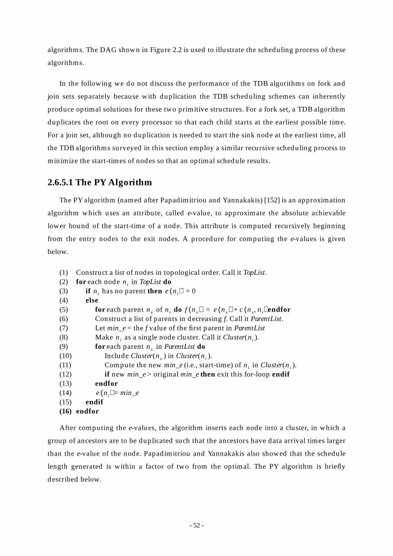
- 52 -

algorithms. The DAG shown in Figure 2.2 is used to illustrate the scheduling process of these

algorithms.

In the following we do not discuss the performance of the TDB algorithms on fork and

join sets separately because with duplication the TDB scheduling schemes can inherently

produce optimal solutions for these two primitive structures. For a fork set, a TDB algorithm

duplicates the root on every processor so that each child starts at the earliest possible time.

For a join set, although no duplication is needed to start the sink node at the earliest time, all

the TDB algorithms surveyed in this section employ a similar recursive scheduling process to

minimize the start-times of nodes so that an optimal schedule results.

2.6.5.1 The PY Algorithm

The PY algorithm (named after Papadimitriou and Yannakakis) [152] is an approximation

algorithm which uses an attribute, called e-value, to approximate the absolute achievable

lower bound of the start-time of a node. This attribute is computed recursively beginning

from the entry nodes to the exit nodes. A procedure for computing the e-values is given

below.

(1) Construct a list of nodes in topological order. Call it TopList.(2) for each node in TopList do(3) if has no parent then = 0(4) else(5) for each parent of do endfor(6) Construct a list of parents in decreasing f. Call it ParentList.(7) Let min_e = the f value of the first parent in ParentList(8) Make as a single node cluster. Call it Cluster( ).(9) for each parent in ParentList do(10) Include Cluster( ) in Cluster( ).(11) Compute the new min_e (i.e., start-time) of in Cluster( ).(12) if new min_e > original min_e then exit this for-loop endif(13) endfor(14) = min_e(15) endif(16) endfor

After computing the e-values, the algorithm inserts each node into a cluster, in which a

group of ancestors are to be duplicated such that the ancestors have data arrival times larger

than the e-value of the node. Papadimitriou and Yannakakis also showed that the schedule

length generated is within a factor of two from the optimal. The PY algorithm is briefly

described below.

ni

ni e ni( )

nx ni f nx( ) e nx( ) c nx ni,( )+=

ni ni

nx

nx ni

ni ni

e ni( )

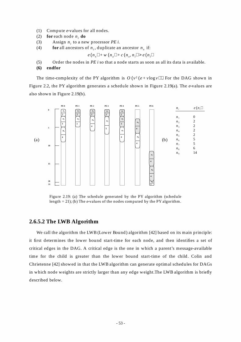
- 53 -

(1) Compute e-values for all nodes.(2) for each node do(3) Assign to a new processor PE i.(4) for all ancestors of , duplicate an ancestor if:

(5) Order the nodes in PE i so that a node starts as soon as all its data is available.(6) endfor

The time-complexity of the PY algorithm is . For the DAG shown in

Figure 2.2, the PY algorithm generates a schedule shown in Figure 2.19(a). The e-values are

also shown in Figure 2.19(b).

2.6.5.2 The LWB Algorithm

We call the algorithm the LWB (Lower Bound) algorithm [42] based on its main principle:

it first determines the lower bound start-time for each node, and then identifies a set of

critical edges in the DAG. A critical edge is the one in which a parent’s message-available

time for the child is greater than the lower bound start-time of the child. Colin and

Chrietenne [42] showed in that the LWB algorithm can generate optimal schedules for DAGs

in which node weights are strictly larger than any edge weight.The LWB algorithm is briefly

described below.

ni

ni

ni nx

e nx( ) w nx( ) c nx ni,( ) e ni( )>+ +

O v2 e v vlog+( )( )

PE 0 PE 1 PE 2 PE 3 PE 4 PE 5 PE 6

0222255614

ni e ni( )

n1

n2

n3

n4

n5

n6

n7

n8

n9

n1

2

n2

3n5

5

n91

n3

3

n7

4

n4

4

0

5

10

15

20

n8

4

n6

4

Figure 2.19: (a) The schedule generated by the PY algorithm (schedulelength = 21); (b) The e-values of the nodes computed by the PY algorithm.

(a) (b)

21

n1

2

n1

2

n1

2

n1

2

n2

3n4

4

n7

4

n8

4

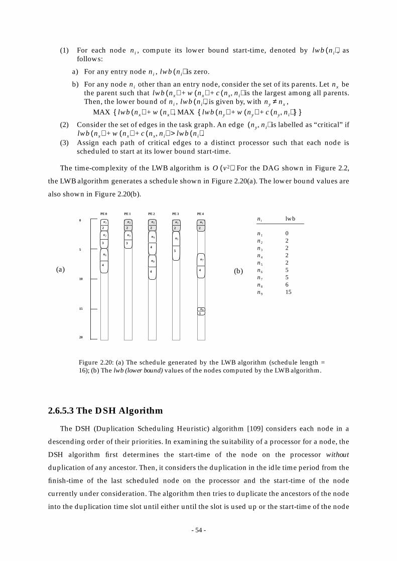
- 54 -

(1) For each node , compute its lower bound start-time, denoted by , asfollows:

a) For any entry node , is zero.

b) For any node other than an entry node, consider the set of its parents. Let bethe parent such that is the largest among all parents.Then, the lower bound of , , is given by, with ,

(2) Consider the set of edges in the task graph. An edge is labelled as “critical” if.

(3) Assign each path of critical edges to a distinct processor such that each node isscheduled to start at its lower bound start-time.

The time-complexity of the LWB algorithm is . For the DAG shown in Figure 2.2,

the LWB algorithm generates a schedule shown in Figure 2.20(a). The lower bound values are

also shown in Figure 2.20(b).

2.6.5.3 The DSH Algorithm

The DSH (Duplication Scheduling Heuristic) algorithm [109] considers each node in a

descending order of their priorities. In examining the suitability of a processor for a node, the

DSH algorithm first determines the start-time of the node on the processor without

duplication of any ancestor. Then, it considers the duplication in the idle time period from the

finish-time of the last scheduled node on the processor and the start-time of the node

currently under consideration. The algorithm then tries to duplicate the ancestors of the node

into the duplication time slot until either until the slot is used up or the start-time of the node

ni lwb ni( )

ni lwb ni( )

ni nxlwb nx( ) w nx( ) c nx ni,( )+ +

ni lwb ni( )MAX lwb nx( ) w nx( ) MAX lwb ny( ) w ny( ) c ny ni,( )+ +{ },+{ }

ny nx≠

ny ni,( )lwb nx( ) w nx( ) c nx ni,( ) lwb ni( )>+ +

O v2( )

PE 0 PE 1 PE 2 PE 3 PE 4

lwb

0222255615

ni

n1

n2

n3

n4

n5

n6

n7

n8

n9

n1

2

n2

3n5

5

n91

n3

3

n7

4

n4

4

0

5

10

15

20

n8

4

n6

4

Figure 2.20: (a) The schedule generated by the LWB algorithm (schedule length =16); (b) The lwb (lower bound) values of the nodes computed by the LWB algorithm.

(a) (b)

n1

2

n1

2

n1

2

n1

2

- 55 -

does not improve. The algorithm is briefly described below.

(1) Compute the static b-level for each node.

Repeat

(2) Let ni be an unscheduled node with the largest static b-level.(3) For each processor P, do:

a) Let the ready time of P, denoted by RT, be the finish-time of the last node on P.Compute the start-time of ni on P and denote it by ST. Then the duplication timeslot on P has length . Let candidate be ni.

b) Consider the set of candidate’s parents. Let nx be the parent of ni which is notscheduled on P and whose message for candidate has the latest arrival time. Try toduplicate nx into the duplication time slot.

c) If the duplication is unsuccessful, then record ST for this processor and tryanother processor; otherwise, let ST be candidate’s new start-time and candidate benx. Goto step b).

(4) Let P’ be the processor that gives the earliest start-time of ni. Schedule ni to P’ andperform all the necessary duplication on P’.


The time-complexity of the DSH algorithm is . For the DAG shown in Figure 2.2,

the DSH algorithm generates a schedule shown in Figure 2.21(a). The steps of scheduling are




2.6.5.4 The BTDH Algorithm

The BTDH (Bottom-Up Top-Down Duplication Heuristic) algorithm [39] is an extension

of the DSH algorithm described above. The major improvement of the BTDH algorithm over

the DSH algorithm is that the algorithm keeps on duplicating ancestors of a node even if the

duplication time slot is totally used up (i.e., the start-time of the node temporarily increases)

with the hope that the start-time will eventually be minimized. That is, the BTDH algorithm

is the same as the DSH algorithm except for step (3)c) of the latter in that the duplication of an

ancestor is considered successful even if the duplication time slot is used up. The process

stops only when the final start-time of the node is greater than before the duplication. The

time-complexity of the BTDH algorithm is also . For the DAG shown in Figure 2.2, the

BTDH algorithm generates the same schedule as the DSH algorithm which is shown in

Figure 2.21(a). The scheduling process is also the same except at step 5 when node is

considered for scheduling on PE 2, the start-time computed by the BTDH algorithm is also 5

ST RT–( )

O v4( )

O v4( )

n6

- 56 -

instead of 6 as computed by the DSH algorithm. This is because the BTDH algorithm does

not stop the duplication process even though the start-time increases.

2.6.5.5 The LCTD Algorithm

The LCTD (Linear Clustering with Task Duplication) algorithm [35] is based on linear

clustering of the DAG. After performing the clustering step, the LCTD algorithm identifies

the edges among clusters that determines the completion time. Then, it tries to duplicate the

parents corresponding to these edges to reduce the start-times of some nodes in the clusters.

The algorithm is described below.


Step PE 0 PE 1 PE 2 PE 3 PE 4 PE 5 Nodes Dup.

1 0* N.C. N.C. N.C. N.C. N.C. NIL2 2* 2 N.C. N.C. N.C. N.C. NIL3 6 2* N.C. N.C. N.C. N.C.4 6 5 2* N.C. N.C. N.C.5 N.C. 5* 6 N.C. N.C. N.C. NIL6 6* N.C. 7 7 N.C. N.C. NIL7 10 9 6 5* N.C. N.C. ,8 10 9 5 9 2* N.C.9 14* 15 N.C. 15 N.C. 15

ni

n1

n4

n2 n1

n3 n1

n6

n8

n7 n1 n2

n5 n1

n9 n7

n1

2

n2

3

n5

5

n91

n3

3

n7

4

n4

4

0

5

10

15

20

n8

4

n6

4

Figure 2.21: (a) The schedule generated by the DSH algorithm (schedulelength = 15); (b) A scheduling trace of the DSH algorithm.

(a)

(b)

n1

2

n1

2

n1

2

n1

2

n2

3

n7

4

- 57 -

(1) Apply the LC algorithm to the DAG to generate a set of linear clusters.(2) Schedule each linear cluster to a distinct processor and let the nodes start as early as

possible on the processors.(3) For each linear cluster do:

a) Let the first node in be .

b) Consider the set of ’s parents. Select the parent that allows the largest reductionof ’s start-time. Duplicate this parent and all the necessary ancestors to .

c) Let be the next node in . Goto step b).(4) Consider each pair of processors. If their schedules have enough common nodes so

that they can be merged without increasing the schedule length, then merge the twoschedules and discard one processor.

The time-complexity of the LCTD algorithm is . For the DAG shown in Figure

2.2, the LCTD algorithm generates a schedule shown in Figure 2.22(a). The steps of

scheduling are given in the table shown in Figure 2.22(b). In the table, the original start-times

of the node on the processors after the linear clustering step are given. In addition, the

improved start-times after duplication are also given.

Ci

Ci nx

nxnx Ci

nx CPi

O v3 vlog( )


Step Org. ST New ST Nodes Dup.

1 0 0 NIL2 10 53 18 164 3 25 7 7 NIL6 6 27 9 5 NIL8 3 29 3 2

ni

n1

n7 n2

n9 n6

n4 n1

n8

n2 n1

n6

n5 n1

n3 n1

n1

2

n2

3n5

5

n91

n3

3

n4

4

0

5

10

15

20

n8

4

n6

4

Figure 2.22: (a) The schedule generated by the LCTD algorithm (schedulelength = 17); (b) A scheduling trace of the LCTD algorithm.

(a)

(b)

n1

2

n1

2

n1

2

n1

2

n2

3

n7

4

n6

4

- 58 -

2.6.5.6 The CPFD Algorithm

The CPFD (Critical Path Fast Duplication) algorithm [4], [6], [111], proposed by Ahmad

and Kwok, is based on partitioning the DAG into three categories: critical path nodes (CPN),

in-branch nodes (IBN) and out-branch nodes (OBN). An IBN is a node from which there is a

path reaching a CPN. An OBN is a node which is neither a CPN nor an IBN. Using this

partitioning of the graph, the nodes can be ordered in decreasing priority as a list called the

CPN-Dominant Sequence. In the following, we first describe the construction of this

sequence.

In a DAG, the CP nodes (CPNs) are the most important nodes since their finish-times

effectively determine the final schedule length. Thus, the CPNs in a task graph should be

considered as early as possible for scheduling in the scheduling process. However, we cannot

consider all the CPNs without first considering other nodes because the start-times of the

CPNs are determined by their parent nodes. Therefore, before we can consider a CPN for

scheduling, we must first consider all its parent nodes. In order to determine a scheduling

order in which all the CPNs can be scheduled as early as possible, we classify the nodes of the

DAG into three categories given in the following definition.

Definition 2.4: In a connected graph, an In-Branch Node (IBN) is a node, which is not a CPN,

and from which there is a path reaching a Critical Path Node (CPN). An Out-Branch Node

(OBN) is a node, which is neither a CPN nor an IBN.

After the CPNs, the most important nodes are IBNs because their timely scheduling can

help reduce the start-times of the CPNs. The OBNs are relatively less important because they

usually do not affect the schedule length. Based on this reasoning, we make a sequence of

nodes called the CPN-Dominant sequence which can be constructed by the following

procedure:

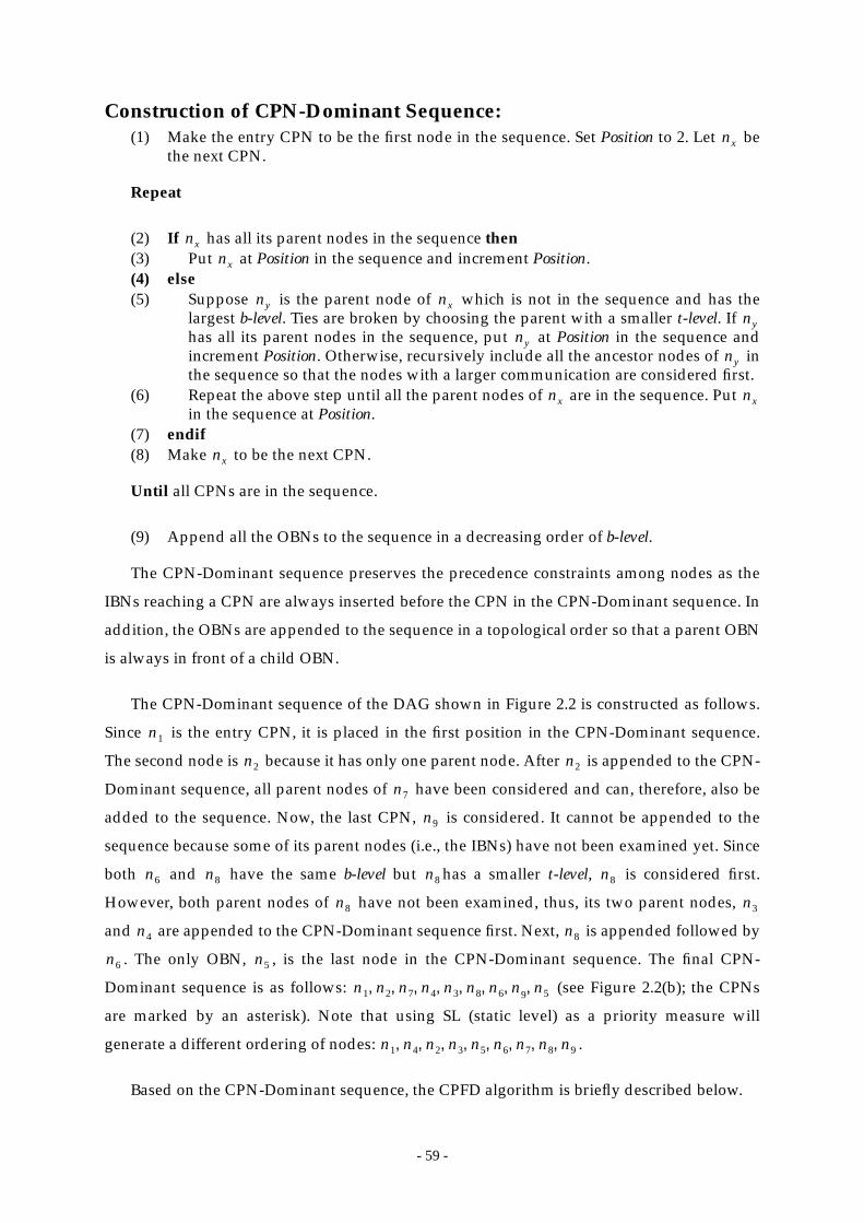
- 59 -

Construction of CPN-Dominant Sequence:(1) Make the entry CPN to be the first node in the sequence. Set Position to 2. Let be

the next CPN.

Repeat

(2) If has all its parent nodes in the sequence then(3) Put at Position in the sequence and increment Position.(4) else(5) Suppose is the parent node of which is not in the sequence and has the

largest b-level. Ties are broken by choosing the parent with a smaller t-level. Ifhas all its parent nodes in the sequence, put at Position in the sequence andincrement Position. Otherwise, recursively include all the ancestor nodes of inthe sequence so that the nodes with a larger communication are considered first.

(6) Repeat the above step until all the parent nodes of are in the sequence. Putin the sequence at Position.

(7) endif(8) Make to be the next CPN.

Until all CPNs are in the sequence.

(9) Append all the OBNs to the sequence in a decreasing order of b-level.

The CPN-Dominant sequence preserves the precedence constraints among nodes as the

IBNs reaching a CPN are always inserted before the CPN in the CPN-Dominant sequence. In

addition, the OBNs are appended to the sequence in a topological order so that a parent OBN

is always in front of a child OBN.

The CPN-Dominant sequence of the DAG shown in Figure 2.2 is constructed as follows.

Since is the entry CPN, it is placed in the first position in the CPN-Dominant sequence.

The second node is because it has only one parent node. After is appended to the CPN-

Dominant sequence, all parent nodes of have been considered and can, therefore, also be

added to the sequence. Now, the last CPN, is considered. It cannot be appended to the

sequence because some of its parent nodes (i.e., the IBNs) have not been examined yet. Since

both and have the same b-level but has a smaller t-level, is considered first.

However, both parent nodes of have not been examined, thus, its two parent nodes,

and are appended to the CPN-Dominant sequence first. Next, is appended followed by

. The only OBN, , is the last node in the CPN-Dominant sequence. The final CPN-

Dominant sequence is as follows: (see Figure 2.2(b); the CPNs

are marked by an asterisk). Note that using SL (static level) as a priority measure will

generate a different ordering of nodes: .

Based on the CPN-Dominant sequence, the CPFD algorithm is briefly described below.

nx

nx

nx

ny nxny

nyny

nx nx

nx

n1

n2 n2

n7

n9

n6 n8 n8 n8

n8 n3

n4 n8

n6 n5

n1 n2 n7 n4 n3 n8 n6 n, 9 n5, , , , , , ,

n1 n4 n2 n3 n5 n6 n7 n8 n9, , , , , , , ,

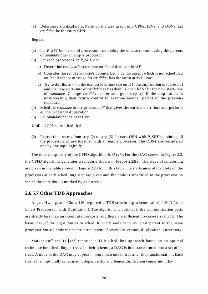
- 60 -

(1) Determine a critical path. Partition the task graph into CPNs, IBNs, and OBNs. Letcandidate be the entry CPN.

Repeat

(2) Let P_SET be the set of processors containing the ones accommodating the parentsof candidate plus an empty processor.

(3) For each processor P in P_SET, do:

a) Determine candidate’s start-time on P and denote it by ST.

b) Consider the set of candidate’s parents. Let m be the parent which is not scheduledon P and whose message for candidate has the latest arrival time.

c) Try to duplicate m on the earliest idle time slot on P. If the duplication is successfuland the new start-time of candidate is less than ST, then let ST be the new start-timeof candidate. Change candidate to m and goto step a). If the duplication isunsuccessful, then return control to examine another parent of the previouscandidate.

(4) Schedule candidate to the processor P’ that gives the earliest start-time and performall the necessary duplication.

(5) Let candidate be the next CPN.

Until all CPNs are scheduled.

(6) Repeat the process from step (2) to step (5) for each OBN with P_SET containing allthe processors in use together with an empty processor. The OBNs are consideredone by one topologically.

The time-complexity of the CPFD algorithm is . For the DAG shown in Figure 2.2,

the CPFD algorithm generates a schedule shown in Figure 2.23(a). The steps of scheduling

are given in the table shown in Figure 2.23(b). In this table, the start-times of the node on the



2.6.5.7 Other TDB Approaches

Anger, Hwang, and Chow [16] reported a TDB scheduling scheme called JLP/D (Joint

Latest Predecessor with Duplication). The algorithm is optimal if the communication costs

are strictly less than any computation costs, and there are sufficient processors available. The

basic idea of the algorithm is to schedule every node with its latest parent to the same

processor. Since a node can be the latest parent of several successors, duplication is necessary.

Markenscoff and Li [132] reported a TDB scheduling approach based on an optimal

technique for scheduling in-trees. In their scheme, a DAG is first transformed into a set of in-

trees. A node in the DAG may appear in more than one in-tree after the transformation. Each

tree is then optimally scheduled independently and hence, duplication comes into play.

O v4( )

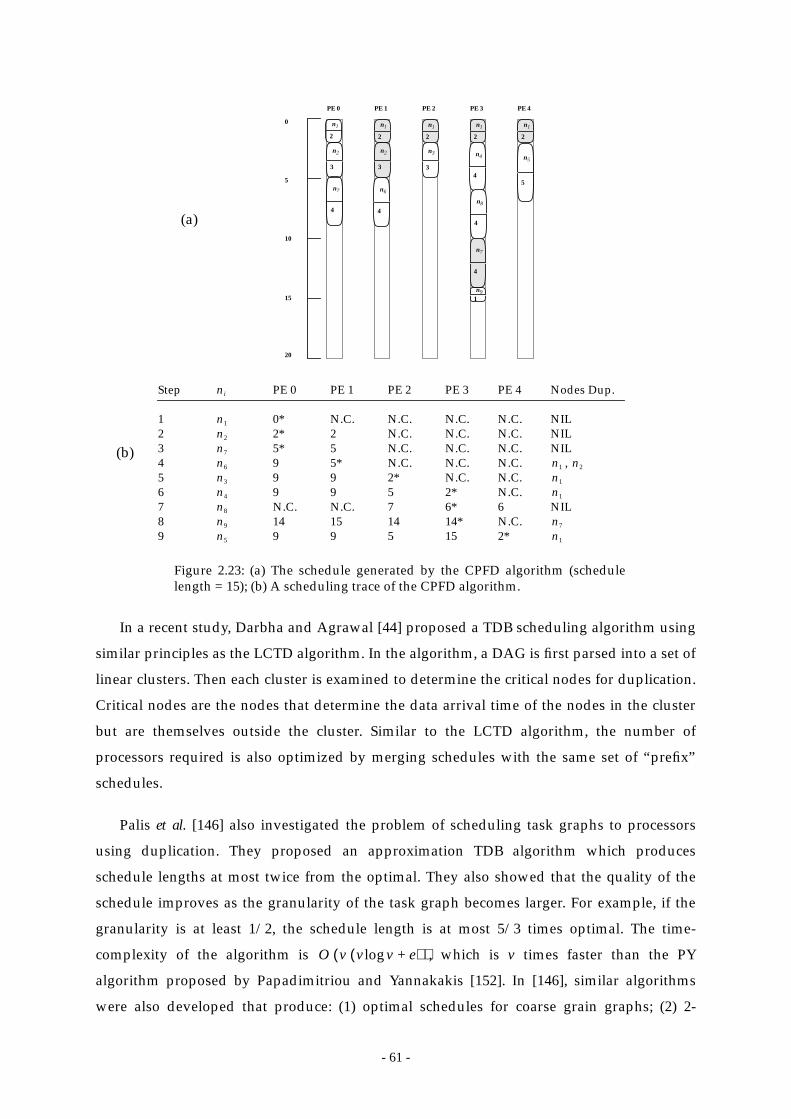
- 61 -

In a recent study, Darbha and Agrawal [44] proposed a TDB scheduling algorithm using

similar principles as the LCTD algorithm. In the algorithm, a DAG is first parsed into a set of

linear clusters. Then each cluster is examined to determine the critical nodes for duplication.

Critical nodes are the nodes that determine the data arrival time of the nodes in the cluster

but are themselves outside the cluster. Similar to the LCTD algorithm, the number of

processors required is also optimized by merging schedules with the same set of “prefix”

schedules.

Palis et al. [146] also investigated the problem of scheduling task graphs to processors

using duplication. They proposed an approximation TDB algorithm which produces

schedule lengths at most twice from the optimal. They also showed that the quality of the

schedule improves as the granularity of the task graph becomes larger. For example, if the

granularity is at least 1/2, the schedule length is at most 5/3 times optimal. The time-

complexity of the algorithm is , which is v times faster than the PY

algorithm proposed by Papadimitriou and Yannakakis [152]. In [146], similar algorithms

were also developed that produce: (1) optimal schedules for coarse grain graphs; (2) 2-


Step PE 0 PE 1 PE 2 PE 3 PE 4 Nodes Dup.

1 0* N.C. N.C. N.C. N.C. NIL2 2* 2 N.C. N.C. N.C. NIL3 5* 5 N.C. N.C. N.C. NIL4 9 5* N.C. N.C. N.C. ,5 9 9 2* N.C. N.C.6 9 9 5 2* N.C.7 N.C. N.C. 7 6* 6 NIL8 14 15 14 14* N.C.9 9 9 5 15 2*

ni

n1

n2

n7

n6 n1 n2

n3 n1

n4 n1

n8

n9 n7

n5 n1

n1

2

n2

3n5

5

n91

n3

3

n7

4

n4

4

0

5

10

15

20

n8

4

n6

4

Figure 2.23: (a) The schedule generated by the CPFD algorithm (schedulelength = 15); (b) A scheduling trace of the CPFD algorithm.

(a)

(b)

n1

2

n1

2

n1

2

n1

2

n2

3

n7

4

O v v v e+log( )( )

- 62 -

optimal schedules for trees with no task duplication; and (3) optimal schedules for coarse

grain trees with no task duplication.

2.6.6 APN Scheduling

In this section we survey the APN class of DAG scheduling algorithms. In particular we

describe in detail four APN algorithms: the MH (Mapping Heuristic) algorithm [50], the DLS

(Dynamic Level Scheduling) algorithm [172], the BU (Bottom Up) algorithm [135], and the

BSA (Bubble Scheduling and Allocation) algorithm [111]. Before we discuss these algorithms,

it is necessary to examine one of the most important issues in APN scheduling—the message

routing issue.

2.6.6.1 The Message Routing Issue

In APN scheduling, a processor network is not necessarily fully-connected and

contention for communication channels need to be addressed. This in turn implies that

message routing and scheduling must also be considered. Recent high-performance

architectures (nCUBE-2 [92], iWarp [92], and Intel Paragon [155]) employ wormhole routing

[43] in which the header flit of a message establishes the path, intermediate flits follow the

path, and the tail flit releases the path. Once the header gets blocked due to link contention,

the entire message waits in the network, occupying all the links it is traversing. Hence, it is

increasingly becoming important to take link contention into account as compared to

distance when scheduling computations onto wormhole-routed systems. Routing strategies

can be classified as either deterministic or adaptive. Deterministic schemes, such as the e-cube

routing for hypercube topology, construct fixed routes for messages and cannot avoid

contention if two messages are using the same link even when other links are free. Yet

deterministic schemes are easy to implement and routing decisions can be made efficiently.

On the other hand, adaptive schemes construct optimized routes for different messages

depending upon the current channel allocation in order to avoid link contention. However,

adaptive schemes are usually more complex as they require much state information to make

routing decisions.

Wang [186] suggested two adaptive routing schemes suitable for use in APN scheduling

algorithms. The first scheme is a greedy algorithm which seeks a locally optimal route for

each message to be sent between tasks. Instead of searching for a path with the least waiting

time, the message is sent through a link which yields the least waiting time among the links

that the processor can choose from for sending a message. Thus, the route is only locally

optimal. Using this algorithm, Wang observed that there are two types of possible blockings:

- 63 -

(i) a later message blocks an earlier message (called LBE blocking), and (ii) an earlier message

blocks a later message (called EBL blocking). LBE blocking is always more costly than EBL

blocking. In the case that several messages are competing for a link and blocking becomes

unavoidable, LBE blockings should be avoided as much as possible. Given this observation,

Wang proposed the second algorithm, called the least blocking algorithm, which works by

trying to avoid LBE blocking. The basic idea of the algorithm is to use Dijkstra’s shortest path

algorithm to arrange optimized routes for messages so as to avoid LBE blockings.

Having determined routes for messages, the scheduling of different messages on the links

is also an important aspect. Dixit-Radiya and Panda [47] proposed a scheme for ordering

messages in a link so as to further minimize the extent of link contention. Their scheme is

based on the Temporal Communication Graph (TCG) which, in addition to task precedence,

captures the temporal relationship of the communication messages. Using the TCG model,

the objective of which is to minimize the contention on the link, the earliest start-times and

latest start-times of messages can be computed. These values are then used to heuristically

schedule the messages in the links.

2.6.6.2 The MH Algorithm

The MH (Mapping Heuristic) algorithm [50] first assigns priorities by computing the SL

of all nodes. A ready node list is then initialized to contain all entry nodes ordered in

decreasing priorities. Each node is scheduled to a processor that gives the smallest start-time.

In calculating the start-time of node, a routing table is maintained for each processor. The

table contains information as to which path to route messages from the parent nodes to the

node under consideration. After a node is scheduled, all of its ready successor nodes are

appended to the ready node list. The MH algorithm is briefly described below.

(1) Compute the SL of each node ni in the task graph.(2) Initialize a ready node list by inserting all entry nodes in the task graph. The list is

ordered according to node priorities, with the highest priority node first.

Repeat

(3) ni ← the first node in the list(4) Schedule ni to the processor which gives the smallest start-time. In determining the

start-time on a processor, all messages from the parent nodes are scheduled androuted by consulting the routing tables associated with each processor.

(5) Append all ready successor nodes of ni, according to their priorities, to the readynode list.

Until the ready node list is empty.

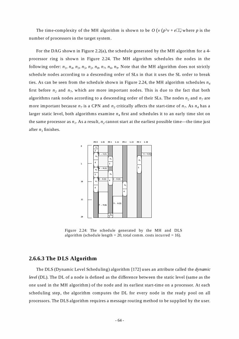
- 64 -

The time-complexity of the MH algorithm is shown to be , where p is the

number of processors in the target system.

For the DAG shown in Figure 2.2(a), the schedule generated by the MH algorithm for a 4-

processor ring is shown in Figure 2.24. The MH algorithm schedules the nodes in the

following order: n1, n4, n3, n5, n2, n8, n7, n6, n9. Note that the MH algorithm does not strictly

schedule nodes according to a descending order of SLs in that it uses the SL order to break

ties. As can be seen from the schedule shown in Figure 2.24, the MH algorithm schedules n4

first before n2 and n7, which are more important nodes. This is due to the fact that both

algorithms rank nodes according to a descending order of their SLs. The nodes n2 and n7 are

more important because n7 is a CPN and n2 critically affects the start-time of n7. As n4 has a

larger static level, both algorithms examine n4 first and schedules it to an early time slot on

the same processor as n1. As a result, n2 cannot start at the earliest possible time—the time just

after n1 finishes.

2.6.6.3 The DLS Algorithm

The DLS (Dynamic Level Scheduling) algorithm [172] uses an attribute called the dynamic

level (DL). The DL of a node is defined as the difference between the static level (same as the

one used in the MH algorithm) of the node and its earliest start-time on a processor. At each

scheduling step, the algorithm computes the DL for every node in the ready pool on all

processors. The DLS algorithm requires a message routing method to be supplied by the user.

O v p3v e+( )( )

Figure 2.24: The schedule generated by the MH and DLSalgorithm (schedule length = 20, total comm. costs incurred = 16).

n1

2

2→ 6 (1)

PE 0

n2

3

n5

5

n91

n3

3

n7

4

n4

4

0

5

10

15

20

n8

4

n6

4

5 ←1 (1)

9 ← 6 (5)7 → 9 (6)

4 → 8 (1)

1 → 3 (1)

2→ 6 (1)

L 01 L 12 L 23 L 30PE 1 PE 2 PE 3

- 65 -

It then computes the earliest start-time of a node on a processor by tentatively scheduling and

routing all messages from the parent nodes using the given routing table. The DLS algorithm

is briefly described below.

(1) Calculate the static level of each node.(2) Initially, the ready node pool includes only the entry nodes.

Repeat

(3) Calculate the earliest start-time for every ready node on each processor. Hence,compute the DL of every node-processor pair by subtracting the earliest start-timefrom the node’s static level.

(4) Select the node-processor pair that gives the largest DL. Schedule the node to thecorresponding processor.

(5) Add the newly ready nodes to the ready pool.


The time-complexity of the DLS algorithm is shown to be , where is the

time-complexity of the message routing algorithm.

For the DAG shown in Figure 2.2(a), the schedule generated by the DLS algorithm for a 4-

processor ring is the same as that generated by the MH algorithm shown in Figure 2.24. The

DLS algorithm also schedules the nodes in the following order: n1, n4, n3, n5, n2, n8, n7, n6, n9.

2.6.6.4 The BU Algorithm

The BU (Bottom-Up) algorithm [135] first determines the critical path (CP) of the DAG

and then assigns all the nodes on the CP to the same processor. Afterwards, the algorithm

assigns the remaining nodes in a reversed topological order of the DAG to the processors.

The node assignment is guided by a load-balancing processor selection heuristic which

attempts to balance the load across all processors. The BU algorithm examines the nodes at

each topological level in a descending order of their b-levels. The b-level of a node is defined as

the largest sum of computation costs and communication costs along a path from the node to

an exit node. After all the nodes are assigned to the processors, the BU algorithm tries to

schedule the communication messages among them using a channel allocation heuristic

which tries to keep the hop count of every message roughly a constant constrained by the

processor network topology. Different network topologies require different channel allocation

heuristics. The BU algorithm is briefly described below.

O v3pf p( )( ) f p( )

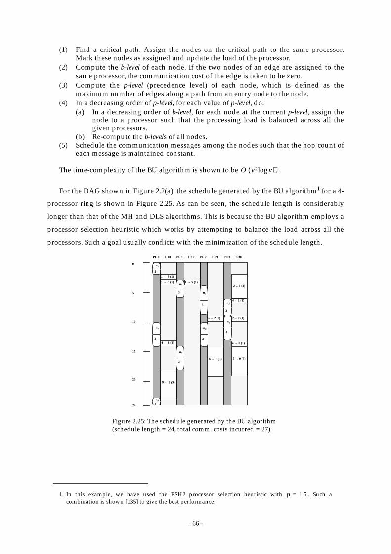
- 66 -

(1) Find a critical path. Assign the nodes on the critical path to the same processor.Mark these nodes as assigned and update the load of the processor.

(2) Compute the b-level of each node. If the two nodes of an edge are assigned to thesame processor, the communication cost of the edge is taken to be zero.

(3) Compute the p-level (precedence level) of each node, which is defined as themaximum number of edges along a path from an entry node to the node.

(4) In a decreasing order of p-level, for each value of p-level, do:(a) In a decreasing order of b-level, for each node at the current p-level, assign the

node to a processor such that the processing load is balanced across all thegiven processors.

(b) Re-compute the b-levels of all nodes.(5) Schedule the communication messages among the nodes such that the hop count of

each message is maintained constant.

The time-complexity of the BU algorithm is shown to be .

For the DAG shown in Figure 2.2(a), the schedule generated by the BU algorithm1 for a 4-

processor ring is shown in Figure 2.25. As can be seen, the schedule length is considerably

longer than that of the MH and DLS algorithms. This is because the BU algorithm employs a

processor selection heuristic which works by attempting to balance the load across all the

processors. Such a goal usually conflicts with the minimization of the schedule length.

1. In this example, we have used the PSH2 processor selection heuristic with . Such acombination is shown [135] to give the best performance.

O v2 vlog( )

ρ 1.5=

n1

2

6← 2 (1)

PE 0

n2

3

n5

5

n91

n3

3

n7

4

n4

4

0

5

10

15

20

n8

4

n6

4

9 ← 8 (5)

4 → 8 (1)

1 → 3 (1)

2→ 7 (1)

L 01 L 12 L 23 L 30PE 1 PE 2 PE 3

24

4 → 8 (1)

6 → 9 (5)6 → 9 (5)

4 ←1 (1)

2 ←1 (4)1 → 5 (1) 1 → 5 (1)

Figure 2.25: The schedule generated by the BU algorithm(schedule length = 24, total comm. costs incurred = 27).

- 67 -

2.6.6.5 The BSA Algorithm

The BSA (Bubble Scheduling and Allocation) algorithm [111], [113], [115] is proposed by

us and is based on an incremental technique which works by improving the schedule

through migration of tasks from one processor to a neighboring processor. The algorithm first

allocates all the tasks to a single processor which has the highest connectivity in the processor

network and is called the pivot processor. In the first phase of the algorithm, the tasks are

arranged in the processor according to the CPN-Dominant sequence discussed earlier in

Section 2.6.5.6. In the second phase of the algorithm, the tasks migrate from the pivot

processor to the neighboring processors if the start-times improve. This task migration

process proceeds in a breadth-first order of the processor network in that after the migration

process is complete for the first pivot processor, one of the neighboring processor becomes

the next pivot processor and the process repeats.

In the following outline of the BSA algorithm, the Build_processor_list() procedure

constructs a list of processors in a breadth-first order from the first pivot processor. The

Serial_injection() procedure constructs the CPN-Dominant sequence of the nodes and injects

this sequence to the first pivot processor.

The BSA Algorithm:(1) Load processor topology and input task graph(2) Pivot_PE ← the processor with the highest degree(3) Build_processor_list(Pivot_PE)(4) Serial_injection(Pivot_PE)(5) while Processor_list_not_empty do(6) Pivot_PE ← first processor of Processor_list(7) for each on Pivot_PE do(8) if ST( , Pivot_PE) > DAT( , Pivot_PE) or Proc(VIP( )) = Pivot_PE then(9) Determine DAT and ST of on each adjacent processor PE’(10) if there exists a PE’ s.t. ST( , PE’) < ST( , Pivot_PE) then(11) Make to migrate from Pivot_PE to PE’(12) Update start-times of nodes and messages(13) else if ST( , PE’) = ST( ,Pivot_PE) and Proc(VIP( )) = PE’ then(14) Make to migrate from Pivot_PE to PE’(15) Update start-times of nodes and messages(16) end if(17) end if(18) end for(19) end while

The time-complexity of the BSA algorithm is .

The BSA algorithm, as shown in Figure 2.26(a), injects the CPN-Dominant sequence to the

ni

ni ni ni

ni

ni ni

ni

ni ni ni

ni

O p2ev( )

- 68 -

first pivot processor PE 0. In the first phase, nodes n1, n2, and n7 do not migrate because they

are already scheduled to start at the earliest possible times. However, as shown in Figure

2.26(b), node n4 migrates to PE 1 because its start-time improves. Similarly, as depicted in

n1

2

PE 0

n2

3

n5

5

n91

n3

3

n7

4

n4

4

0

5

10

15

20

n8

4

n6

4

L 01 L 12 L 23 L 30PE 1 PE 2 PE 3

25

(c)

30

n1

2

PE 0

n2

3

n5

5

n91

n3

3

n7

4

n4

4

0

5

10

15

20

n8

4

n6

4

L 01 L 12 L 23 L 30PE 1 PE 2 PE 3

25

30

1 → 4 (1)

8 ← 4 (1)

n1

2

PE 0

n2

3

n5

5

n91

n3

3

n7

4

n4

4

0

5

10

15

20

n8

4

n6

4

L 01 L 12 L 23 L 30PE 1 PE 2 PE 3

23

1 → 4 (1)

8 ← 4 (1)

3 ←1 (1)

3 → 8 (1)

n1

2

PE 0

n2

3

n5

5

n91

n3

3

n7

4

n4

4

0

5

10

15

20

n8

4n6

4

L 01 L 12 L 23 L 30PE 1 PE 2 PE 3

23

1 → 4 (1) 3 ←1 (1)

3 → 8 (1)3 → 8 (1)

9 ← 8 (5)

(a) (b)

(d)

Figure 2.26: Intermediate schedules produced by BSA after (a) serial injection (schedulelength = 30, total comm. cost = 0); (b) n4 migrates from PE 0 to PE 1 (schedule length = 26,total comm. cost = 2); (c) n3 migrates from PE 0 to PE 3 (schedule length = 23, total comm.cost = 4); (d) n8 migrates from PE 0 to PE 1 (schedule length = 22, total comm. cost = 9).

- 69 -

Figure 2.26(c), node n3 also migrates to a neighboring processor PE 3. Figure 2.26(d) shows

the intermediate schedule after n8 migrates to PE 1 following its VIP n4. Similarly, n6 also

migrates to PE 3 following its VIP n3, as shown in Figure 2.27(a). The last CPN, n9, migrates to

PE 1 to which its VIP n8 is scheduled. Such migration allows the only OBN n5 to bubble up.

The resulting schedule is shown in Figure 2.27(b). This is the final schedule as no more nodes

can improve the start-time through migration.

2.6.6.6 Other APN Approaches

Kon’ya and Satoh [107] reported an APN scheduling algorithm for the hypercube

architectures. Their algorithm, called the LST (Latest Starting Time) algorithm, works by

using a list scheduling approach in that the priorities of nodes are first computed and a list is

constructed based on these priorities. The priority of a node is defined as its latest starting

time, which is determined before scheduling starts. Thus, the list is static and does not

capture the dynamically changing importance of nodes, which is crucial in APN scheduling.

In a later study, Selvakumar and Murthy [161] reported an APN scheduling scheme

which is an extension of Sih and Lee’s DLS algorithm. The distinctive new feature in their

algorithm is that it exploits schedule holes in processors and communication links in order to

produce better schedules. Essentially, it differs from the DLS algorithm in two respects: (i) the

(b)(a)

Figure 2.27: (a) Intermediate schedule produced by BSA after n6 migrates from PE 0 to PE 3(schedule length = 22, total comm. cost = 15); (b) final schedule produced by BSA after n9migrates from PE 0 to PE 1 and n5 is bubbled up (schedule length = 16, total comm. cost = 21).

n1

2

PE 0

n2

3

75

5

n91

n3

3

n7

4

n4

4

0

5

10

15

20

n8

4

n6

4

L 01 L 12 L 23 L 30PE 1 PE 2 PE 3

23

1 → 4 (1) 3 ←1 (1)

3 → 8 (1)3 → 8 (1)

9 ← 8 (5)

6 ← 2 (1)

6 → 9 (5)

n1

2

PE 0

n2

3

n5

5

n91

n3

3

n7

4

n4

4

0

5

10

15

16

n8

4

n6

4

L 01 L 12 L 23 L 30PE 1 PE 2 PE 3

1 → 4 (1) 3 ←1 (1)

3 → 8 (1)3 → 8 (1)

7 → 9 (6)

6 ← 2 (1)

9 ← 6 (5)9 ← 6 (5)

- 70 -

way in which the priority of a task with respect to a processor in a partial schedule; and (ii)

the way in which a task and all communications from its parents are scheduled. The priority

of a node is modified to be the difference between the static level and the earliest finish-time.

During the scheduling of a node, a router is used to determine the best possible path between

the processors that need communication. In their simulation study, the improved scheduling

algorithm outperformed both the DLS algorithm and the MH algorithm.

2.6.7 Scheduling in Heterogeneous Environments

Heterogeneity has been shown to be an important attribute in improving the

performance of multiprocessors [54], [59], [136], [167], [169], [171], [188]. In parallel

computations, the serial part is the bottleneck, according to Amhdal’s law [15]. In

homogeneous multiprocessors, if one or more faster processors are used to replace a set of

cost-equivalent processors, the serial computations and other critical computations can be

scheduled to such faster processors and performed at a greater rate so that speedup can be

increased.

As we have seen in earlier parts of this section, most DAG scheduling approaches assume

the target system is homogeneous. Introducing heterogeneity into the model inevitably

makes the problem more complicated to handle. This is because the scheduling algorithm has

to take into account the different execution rate of different processors when computing the

potential start-times of tasks on the processors. Another complication is that the resulting

schedule for a given heterogeneous system immediately becomes invalid if some of the

processing elements are replaced even though the number of processors remain the same.

This is because the scheduling decisions are made not only on the number of processors but

also on the capability of the processors.

Static scheduling targeted for heterogeneous environments was unexplored until

recently. Menasce et al. [137], [138], [139], [140] investigated the problem of scheduling

computations to heterogeneous multiprocessing environments. The heterogeneous

environment was modeled as a system with one fast processor plus a number of slower

processors. In their study, both dynamic and static scheduling schemes were examined but

nevertheless DAGs without communication are used to model computations [14]. Markov

chains were used to analyze the performance of different scheduling schemes. In their

findings, out of all the static scheduling schemes, the LTF/MFT (Largest Task First/

Minimizing finish-time) significantly outperformed all the others including WL (Weighted

Level), CPM (Critical Path Method) and HNF (Heavy Node First). The LTF/MFT algorithm

- 71 -

works by picking the largest task from the ready tasks list and schedules it to the processor

which allows the minimum finish-time, while the other three strategies select candidate

processor based on the execution time of the task. Thus, based on their observations, an

efficient scheduling algorithm for heterogeneous systems should concentrate on reducing the

finish-times of tasks. Nonetheless, if communication delays are also considered, different

strategies may be needed.

2.6.8 Mapping Clusters to Processors

As discussed earlier, mapping of clusters to physical processors is necessary for UNC

scheduling when the number of clusters is larger than the number of physical processors.

However, the mapping of clusters to processors is a relatively unexplored research topic

[121]. In the following we discuss a number of approaches reported in the literature.

Upon obtaining a schedule by using the EZ algorithm, Sarkar [160] used a list-scheduling

based method to map the clusters to physical processors. In the mapping algorithm, each task

is considered in turn according to the static level. A processor is allocated to the task if it

allows the earliest execution, then the whole cluster containing the task is also assigned to

that processor and all the member tasks are marked as assigned. In this scheme, two clusters

can be merged to a single processor but a cluster is never cracked. Furthermore, the allocation

of channels to communication messages was not considered.

Kim and Browne [105] also proposed a mapping scheme for the UNC schedules obtained

from their LC algorithm. In their scheme, the linear UNC clusters are first merged so that the

number of clusters is at most the same as the number of processors. Two clusters are

candidates for merging if one can start after another finishes, or the member tasks of one

cluster can be merged into the idle time slots of another cluster. Then a dominant request tree

(DRT) is constructed from the UNC schedule which is a cluster graph. The DRT consists of

the connectivity information of the schedule and is, therefore, useful for the mapping stage in

which two communicating UNC clusters attempt to be mapped to two neighboring

processors, if possible. However, if for some clusters this connectivity mapping heuristic fails,

another two heuristics, called perturbation mapping and foster mapping, are invoked. For both

mapping strategies, a processor is chosen which has the most appropriate number of

channels among currently unallocated processors. Finally, to further optimize the mapping, a

restricted pairwise exchange step is called for.

Wu and Gajski [189] also suggested a mapping scheme for assigning the UNC clusters

generated in scheduling to processors. They realized that for best mapping results, a

- 72 -

dedicated traffic scheduling algorithm that balances the network traffic should be used.

However, traffic scheduling requires flexible-path routing, which incurs higher overhead.

Thus, they concluded that if network traffic is not heavy, a simpler algorithm which

minimizes total network traffic can be used. The algorithm they used is a heuristic algorithm

designed by Hanan and Kurtzberg [83] to minimize the total communication traffic. The

algorithm generates an initial assignment by a constructive method and the assignment is

then iteratively improved to obtain a better mapping.

Yang and Gerasoulis [191] employed a work profiling method for merging UNC clusters.

The merging process proceeds by first sorting the clusters in an increasing order of aggregate

computational load. Then a load balancing algorithm is invoked to map the clusters to the

processors so that every processor has about the same load. To take care of the topology of the

underlying processor network, the graph of merged clusters are then mapped to the network

topology using Bokhari’s algorithm.

Yang, Bic, and Nicolau [195] reported an algorithm for mapping cluster graphs to

processor graphs which is suitable for use as the post-processing step for BNP scheduling

algorithms. The mapping scheme is not suitable for UNC scheduling because it assumes the

scheduling algorithm has already produced a number of clusters which is less than or equal

to the number of processors available. The objective of the mapping method is to reduce

contention and optimize the schedule length when the clusters are mapped to a topology

which is not fully-connected as assumed by the BNP algorithms. The idea of the mapping

algorithm is based on determining a set of critical edges, each of which is assigned a single

communication link. Substantial improvement over random mapping was obtained in their

simulation study.

In a recent study, Liou and Palis [126] investigated the problem of mapping clusters to

processors. One of the major objectives of their study was to compare the effectiveness of

one-phase scheduling (i.e., BNP scheduling) to that of the two-phase approach (i.e., UNC

scheduling followed by clusters mapping). To this end, they proposed a new UNC algorithm

called CASS-II (Clustering And Scheduling System II), which was applied to randomly

generated task graphs in an experimental study using three clusters mapping schemes,

namely, the LB (load-balancing) algorithm, the CTM (communication traffic minimizing)

algorithm and the RAND (random) algorithm. The LB algorithm uses processor workload as

the criterion of matching clusters to processors. By contrast, the CTM algorithm tries to

minimize the communication costs between processors. The RAND algorithm simply makes

random choices at each mapping step. To compare the one-phase method with the two-phase

- 73 -

method, in one set of test cases the task graphs were scheduled using CASS-II with the three

mapping algorithms while in the other set using the mapping algorithms alone. Liou and

Palis found that two-phase scheduling is better than one-phase scheduling in that the

utilization of processors in the former is more efficient than the latter. Futhermore, they found

that the LB algorithm finds significantly better schedules than the CTM algorithm.

2.7 Summary and Concluding Remarks

In this chapter we have presented the background of the static scheduling problem. We

first introduced the DAG model and the multiprocessor model, followed by the problem

statement. In the DAG model, a node denotes an atomic program task and an edge denotes

the communication and data dependency between two program tasks. Each node is labeled a

weight denoting the amount of computational time required by the task. Each edge is also

labeled a weight denoting the amount of communication time required. The target

multiprocessor systems is modeled as a network of processing elements (PEs), each of which

comprises a processor and a local memory unit, so that communication is achieved solely by

message-passing. The objective of scheduling is to minimize the schedule length by properly

allocating the nodes to the PEs and sequencing their start-times so that the precedence

constraints are not violated.

We also presented a survey of scheduling algorithms. Before introducing the survey, we

presented a scrutiny of the NP-completeness results of various simplified variants of the

problem, thereby illustrating that static scheduling is a hard optimization problem. As the

problem is intractable even for moderately general cases, heuristic approaches are commonly

sought. To better understand the design of the heuristic scheduling schemes, we have also

described and explained a set of basic techniques used in most algorithms. With these

techniques the task graph structure is carefully exploited to determine the relative

importance of the nodes in the graph. More important nodes get a higher consideration

priority for scheduling first. An important structure in a task graph is the critical path (CP), a

longest path in the graph. The nodes of the CP can be identified by the nodes’ b-level and t-

level. In order to put the representative work with different assumptions reported in the

literature in a unified framework, we described a taxonomy of scheduling algorithms which

classifies the algorithms into four categories: the UNC (unbounded number of clusters)

scheduling, the BNP (bounded number of processors) scheduling, the TDB (task duplication

based) scheduling, and APN (arbitrary processor network) scheduling. Analytical results as

well as scheduling examples have been shown to illustrate the functionality and

characteristics of the surveyed algorithms. Tasks scheduling for heterogeneous systems,

- 74 -

which are widely considered as promising platforms for high-performance computing, is

briefly discussed. As a post-processing step of some scheduling algorithms, the mapping

process is also examined.

- 75 -

Chapter 3

A Low Complexity Scheduling Algorithm

3.1 Introduction

While it is understood that static scheduling is done off-line and therefore some extra time

can be afforded in generating a better solution, the time-complexity of an algorithm is an

important issue from a practical point of view. As mentioned in Chapter 2, there are a large

number of scheduling heuristics suggested in the literature. However, while many of them

can generate good solutions, few have a low time-complexity. As such most of the algorithms

may be inapplicable for practical purposes. In a recent study [9], we compared 21 recently

reported algorithms and made a number of observations. For example, we found that an

algorithm may take more than an hour to produce a schedule for a DAG with 1,000

nodes, a typical size for many applications. Taking such a large amount of time to generate a

solution for an application is a major hurdle in incorporating these algorithms in

parallelizing compilers. On the other hand, some algorithms have low time-complexity but

their solution quality is not satisfactory [9]. Thus, an algorithm which meets the conflicting

goals of high performance and low time-complexity is highly desired. In this regard, Yang

and Gerasoulis [193] proposed some novel techniques for reducing the time-complexity of

scheduling algorithms. Our objective is to design an algorithm that has a comparable or

lower complexity while producing better solutions.

In this chapter, we propose a low complexity BNP scheduling algorithm called Fast

Assignment using Search Technique (FAST) which has time-complexity. The FAST

algorithm is based on an effective search technique [117]. The linear-time algorithm first

generates an initial solution and then refines it using a random neighborhood search

technique. Random search based algorithms have been proposed and applied to various

problems with good results [81], [98], [127], [149], [189].

In addition to simulation studies, the FAST algorithm is evaluated using a prototype

computer-aided parallelization and scheduling tool called CASCH (Computer-Aided

O v3( )

O e v+( )

- 76 -

SCHeduling), with real applications running on the Intel Paragon. The FAST algorithm

outperforms numerous previous algorithms while its execution times are dramatically

smaller. Indeed, based on our experimental results, the FAST algorithm is the fastest

scheduling algorithm known to us. To further reduce the running time of the algorithm, we

propose a parallelization of the FAST algorithm. The resulting algorithm, called the Parallel

FAST (PFAST) algorithm, is evaluated using random task graphs for which optimal solutions

are known. The PFAST algorithm generated optimal solutions for a significant portion of the

test cases and close-to-optimal solutions for the other cases. Furthermore, the algorithm is

scalable in that it exhibits an almost linear speedup. The PFAST algorithm is therefore an

attractive choice for generating high quality schedules in a parallel processing environment

under running time constraints.

This chapter is organized as follows. In Section 3.2, we first discuss the trade-off between

more complexity and better performance. In the same section we introduce the idea of using

neighborhood search to improve the scheduling performance. In Section 3.3 we describe the

proposed FAST and PFAST algorithms. Their design principles are also described in detail. In

Section 3.4 we present a detailed example to illustrate the functionality of the algorithms.

Section 3.5 contains the performance results of the FAST and PFAST algorithms as well as a

comparison with other algorithms. The final section concludes this chapter.

3.2 Scheduling Using Neighborhood Search

Traditional DAG scheduling algorithms attempt to minimize the schedule length through

local optimizations of the scheduling of individual nodes. However, most of the local

optimization strategies are not effective in general in that most algorithms minimize the start-

time of a node at each scheduling step (see Chapter 2). These algorithms differ only in the

way of selecting a node for scheduling. Some of them construct a list of nodes before

scheduling starts (as in the list scheduling algorithms like the MCP algorithm [189]) while

some of them dynamically select nodes for scheduling (e.g., the DLS algorithm [172]).

However, in an optimal schedule, some nodes may have to start later than the earliest

possible time. Thus, like most algorithms of a greedy nature, these scheduling algorithms

cannot avoid making a local decision which may lead to a sub-optimal schedule. As

backtracking is not employed in order not to incur high complexity, a mistake made in an

earlier step may not be remedied in later steps.

Hitherto there are a few scheduling algorithms that attempt to make decisions based on

more global information. For instance, in the DCP algorithm [114], the start-time of a node

- 77 -

depends on the anticipated start-time of its critical child and therefore, may not be the earliest

possible. However, due to the horizon effect, which means that sub-optimal decisions are

inevitable no matter how far you look ahead, it is nonetheless unavoidable to make a locally

optimal decision which is in fact globally sub-optimal. For instance, as we have seen in the

example schedules produced by the MCP and DCP algorithms shown earlier in Figure 2.15

and Figure 2.12 in Chapter 2 respectively, a deterministic heuristic may be trapped by a

locally optimal decision which may turn out eventually to be sub-optimal.

To obtain an optimal schedule, we have to tackle the scheduling problem from a global

perspective. However, global information is usually obtained at the expense of high time-

complexity. To obtain such global information, we can use the characteristics of the task

graph such as the graph structure and the relative magnitudes of the node and edge weights.

Using such attributes, we can decide, from a global point of view, which nodes in the task

graph deserve special attention so that eventually an optimal schedule can be constructed.

For instance, some previously reported scheduling algorithms is based on a global

characteristic structure of the task graph, namely, the critical path (CP). A CP is a path with the

maximum sum of node and edge weights or simply, the maximum length. Thus, if an

unlimited number of processors are available, the length of the CP provides an upper bound

on the schedule length. In light of this attractive property, most scheduling algorithms assign

higher priorities to nodes of the CP for scheduling. For example, in the list scheduling

algorithms, a node on the CP occupies an earlier position in the scheduling list. However,

while the CP length provides an upper bound on the schedule length, making all the nodes

on the CP start at the earliest possible time does not guarantee an optimal schedule. In fact, if

the edge weights are much larger than the node weights in general, such a strategy can even

lead to a bad schedule [9].

The crux for getting around the problem lies in the fact that in the course of scheduling,

the CP can change—the set of nodes constituting the CP at a certain scheduling step may be

different from that at an earlier step. Indeed, the algorithms that dynamically selects nodes

for scheduling such as the MD, DLS, DSC and DCP algorithms (discussed in Chapter 2), are

designed based on this observation. These algorithms attempt to track the most updated CP

after each scheduling step and by doing so, they are much less sensitive to the relative

magnitudes of the node and edge weights [9]. But as we have discussed earlier, dynamically

tracking the CP while making every node start at the earliest time can lead to a formidable

time-complexity. The only exception—the DSC algorithm [193]—avoids incurring high

complexity by deferring the consideration of scheduling the nodes on the CP. Unfortunately,

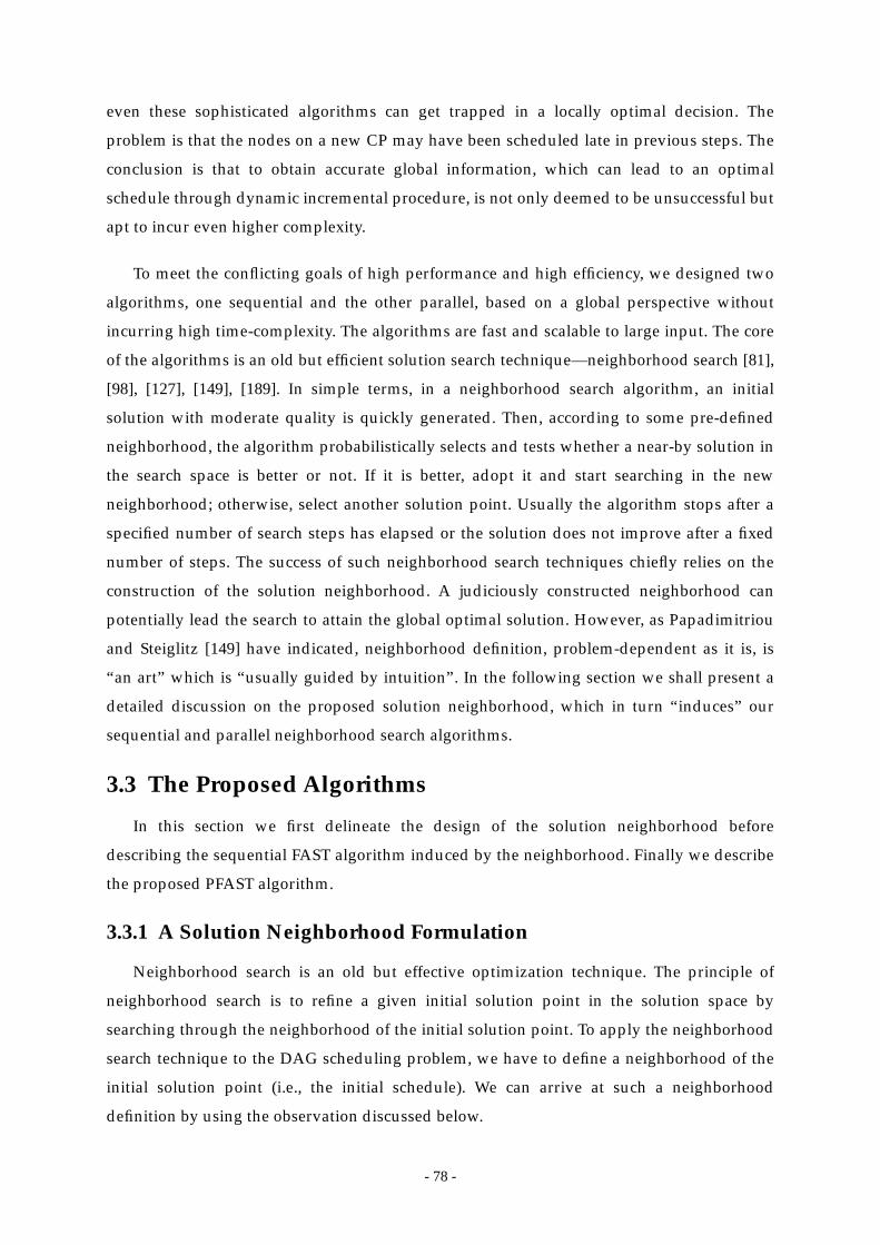
- 78 -

even these sophisticated algorithms can get trapped in a locally optimal decision. The

problem is that the nodes on a new CP may have been scheduled late in previous steps. The

conclusion is that to obtain accurate global information, which can lead to an optimal

schedule through dynamic incremental procedure, is not only deemed to be unsuccessful but

apt to incur even higher complexity.

To meet the conflicting goals of high performance and high efficiency, we designed two

algorithms, one sequential and the other parallel, based on a global perspective without

incurring high time-complexity. The algorithms are fast and scalable to large input. The core

of the algorithms is an old but efficient solution search technique—neighborhood search [81],

[98], [127], [149], [189]. In simple terms, in a neighborhood search algorithm, an initial

solution with moderate quality is quickly generated. Then, according to some pre-defined

neighborhood, the algorithm probabilistically selects and tests whether a near-by solution in

the search space is better or not. If it is better, adopt it and start searching in the new

neighborhood; otherwise, select another solution point. Usually the algorithm stops after a

specified number of search steps has elapsed or the solution does not improve after a fixed

number of steps. The success of such neighborhood search techniques chiefly relies on the

construction of the solution neighborhood. A judiciously constructed neighborhood can

potentially lead the search to attain the global optimal solution. However, as Papadimitriou

and Steiglitz [149] have indicated, neighborhood definition, problem-dependent as it is, is

“an art” which is “usually guided by intuition”. In the following section we shall present a

detailed discussion on the proposed solution neighborhood, which in turn “induces” our

sequential and parallel neighborhood search algorithms.

3.3 The Proposed Algorithms

In this section we first delineate the design of the solution neighborhood before

describing the sequential FAST algorithm induced by the neighborhood. Finally we describe

the proposed PFAST algorithm.

3.3.1 A Solution Neighborhood Formulation

Neighborhood search is an old but effective optimization technique. The principle of

neighborhood search is to refine a given initial solution point in the solution space by

searching through the neighborhood of the initial solution point. To apply the neighborhood

search technique to the DAG scheduling problem, we have to define a neighborhood of the

initial solution point (i.e., the initial schedule). We can arrive at such a neighborhood

definition by using the observation discussed below.

- 79 -

We can visualize some global features, which characterize the final schedules, from the

example schedules of the task graph (see Figure 2.2(a) in Chapter 2) produced by the MCP

and DCP algorithms shown earlier in Figure 2.15 and Figure 2.12 in Chapter 2, respectively.

Let us consider the schedule produced by the MCP algorithm. The node determines the

schedule length. It cannot start earlier because of the dependency from , which, in turn

depends on . Repeat this backward tracing and we finally obtain a path: .

This path determines the schedule length in that all the nodes on the path cannot be made to

start later without increasing the schedule length. That is, they are immobile. Let us define

such a path as the final critical path (FCP). Now consider the schedule produced by the DCP

algorithm. One FCP is . Note that FCP is not unique— is also a

FCP. By our definition, the nodes on a FCP cannot be pushed downward but they can be

pulled upward if some blocking-nodes are disposed to other processors. Indeed, let us consider

the schedule produced by MCP again. If is transferred from PE 0 to PE 2, the schedule

length will be improved. This is because then and hence and can start earlier.

Consequently can also start earlier and the schedule length is shortened.

Based on the above observation, a simple neighborhood point of a schedule in the

solution space can be defined as another schedule which is obtained by transferring a node

from a processor to another processor. In the DAG scheduling problem, one method of

improving the schedule length is to transfer a blocking-node from one processor to another.

The notion of blocking is simple—a node is called blocking if removing it from its original

processor can make the succeeding nodes start earlier. In particular, we are interested in

transferring the nodes that block the CPNs because the CPNs are the more important nodes.

However, high complexity will result if we attempt to locate the actual blocking-nodes on all

the processors. Thus, in our approach, we only generate a list of potential blocking-nodes

which are the nodes that may block the CPNs. Again, to maintain a low complexity, the

blocking-nodes list is static and is constructed before the search process starts. A natural

choice of blocking-nodes list is the set of IBNs and OBNs (with respect to an initial CP)

because these nodes have the potential to block the CPNs in the processors. In the schedule

refinement phase, the blocking-nodes list defines the neighborhood that the random search

process will explore. The size of such a neighborhood is because there are

blocking-nodes and p processors.

3.3.2 The Sequential FAST Algorithm

To generate an initial schedule, we employ the traditional list scheduling approach—

construct a list and schedule the nodes on the list one by one to the processors. The list is

n9

n6

n2 n1 n2 n6 n9, , ,{ }

n1 n2 n7 n9, , ,{ } n1 n4 n8 n9, , ,{ }

n4

n2 n6 n7

n9

O vp( ) O v( )

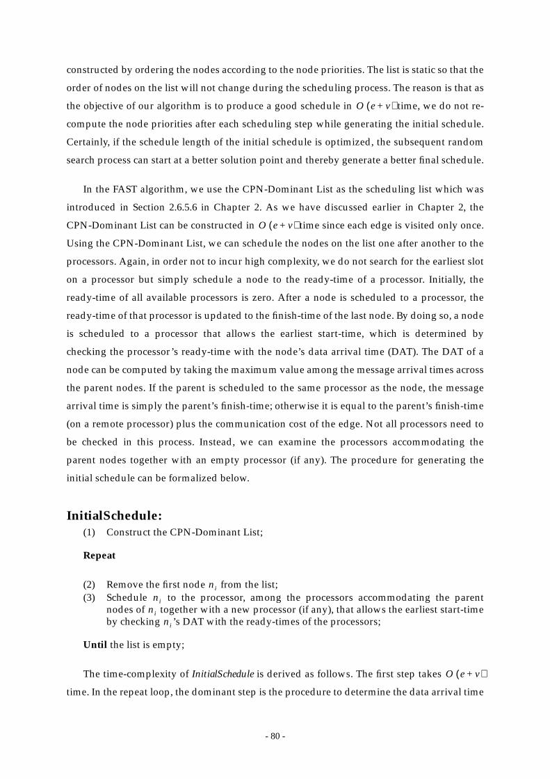
- 80 -

constructed by ordering the nodes according to the node priorities. The list is static so that the

order of nodes on the list will not change during the scheduling process. The reason is that as

the objective of our algorithm is to produce a good schedule in time, we do not re-

compute the node priorities after each scheduling step while generating the initial schedule.

Certainly, if the schedule length of the initial schedule is optimized, the subsequent random

search process can start at a better solution point and thereby generate a better final schedule.

In the FAST algorithm, we use the CPN-Dominant List as the scheduling list which was

introduced in Section 2.6.5.6 in Chapter 2. As we have discussed earlier in Chapter 2, the

CPN-Dominant List can be constructed in time since each edge is visited only once.

Using the CPN-Dominant List, we can schedule the nodes on the list one after another to the

processors. Again, in order not to incur high complexity, we do not search for the earliest slot

on a processor but simply schedule a node to the ready-time of a processor. Initially, the

ready-time of all available processors is zero. After a node is scheduled to a processor, the

ready-time of that processor is updated to the finish-time of the last node. By doing so, a node

is scheduled to a processor that allows the earliest start-time, which is determined by

checking the processor’s ready-time with the node’s data arrival time (DAT). The DAT of a

node can be computed by taking the maximum value among the message arrival times across

the parent nodes. If the parent is scheduled to the same processor as the node, the message

arrival time is simply the parent’s finish-time; otherwise it is equal to the parent’s finish-time

(on a remote processor) plus the communication cost of the edge. Not all processors need to

be checked in this process. Instead, we can examine the processors accommodating the

parent nodes together with an empty processor (if any). The procedure for generating the

initial schedule can be formalized below.

InitialSchedule:(1) Construct the CPN-Dominant List;

Repeat

(2) Remove the first node from the list;(3) Schedule to the processor, among the processors accommodating the parent

nodes of together with a new processor (if any), that allows the earliest start-timeby checking ’s DAT with the ready-times of the processors;

Until the list is empty;

The time-complexity of InitialSchedule is derived as follows. The first step takes

time. In the repeat loop, the dominant step is the procedure to determine the data arrival time

O e v+( )

O e v+( )

ni

nini

ni

O e v+( )

- 81 -

of a node. The cumulative time-complexity of this step throughout the execution of the repeat

loop is also because each edge is visited once. Thus, the overall time-complexity of

InitialSchedule is also .

Given the procedure InitialSchedule we can present the sequential version of our

neighborhood search algorithm. In order to avoid being trapped in a local optimal solution,

we incorporate a probabilistic jump procedure in the algorithm. The FAST algorithm is

outlined below.

The FAST Algorithm:(1) NewSchedule = InitialSchedule(2) Construct the blocking-nodes list which contains all the IBNs and OBNs;(3) BestSL = infinity; searchcount = 0;(4) repeat(5) searchstep = 0; counter = 0;(6) do { /* neighborhood search */(7) Pick a node randomly from the blocking-nodes list;(8) Pick a processor P randomly;(9) Transfer to P;(10) If schedule length does not improve, transfer back to its original processor

and increment counter; otherwise, set counter to 0;(11) } while (searchstep++ < MAXSTEP and counter < MARGIN);(12) if BestSL > SL(NewSchedule) then(13) BestSchedule = NewSchedule(14) BestSL = SL(NewSchedule)(15) endif(16) NewSchedule = Randomly pick a node from the FCP and transfer it to another

processor; /* probabilistic jump */(17) until (searchcount++ > MAXCOUNT);

The total number of search-steps is . While the number of

search steps in each iteration is bounded by MAXSTEP, the algorithm will also terminate

searching and proceed to the step of probabilistic jump if the solution does not improve

within a specified number of steps, denoted as MARGIN. This is done in order to further

enhance the expected efficiency of the algorithm.

The reason of making MAXSTEP, MARGIN, and MAXCOUNT as constants is two-fold.

First, the prime objective in the design of the algorithm is to keep the time-complexity low

even when the size of the input graph is huge. Second, the major strength of the FAST

algorithm lies in its ability to generate a good initial solution by using the CPN-Dominant

List. As such, the likelihood of improving the initial solution dramatically by using large

number of search steps is not high. Thus, we fix MARGIN to be 2, MAXSTEP to be 8, and

O e v+( )

O e v+( )

ni

ni

ni

MAXSTEP MAXCOUNT×

- 82 -

MAXCOUNT to be 64 based on our experimental results which will be described in detail in

Section 3.5.1.

The time-complexity of the sequential FAST algorithm is determined as follow. As

discussed earlier, the procedure InitialSchedule() takes time. The blocking-nodes list

can be constructed in time as the IBNs and OBNs are already identified in the

procedure InitialSchedule(). In the main loop, the node transferring step takes time

since we have to re-visit all the edges once after transferring the node to a processor in the

worst case. Thus, the overall time-complexity of the sequential algorithm is .

3.3.3 The PFAST Algorithm

In the parallel version of the algorithm, we partition the blocking-nodes set into q subsets

where q is the number of available physical processing elements (PPEs), on which the PFAST

algorithm is executed. Each PPE then performs a neighborhood search using its own

blocking-nodes subset. The PPEs communicate periodically to exchange the best solution

found thus far and start new search steps based on the best solution. The period of

communication for the PPEs is set to be T number of search-steps, which follows an

exponentially decreasing sequence: initially , then , , and so on, where

. The rationale is that at early stages of the search, exploration is more

important than exploitation. The PPEs should, therefore, work independently for longer

period of time. However, at final stages of the search, exploitation is more important so that

the PPEs should communicate more frequently.

The PFAST algorithm is outlined below.

The PFAST Algorithm:(1) if myPPE() == master then(2) Determine the initial schedule;(3) Construct the blocking-nodes set;(4) Partition the blocking-nodes set into q subsets which are ordered topologically;(5) endif(6) Every PPE receives a blocking-nodes subset and the initial schedule;(7) repeat(8)(9) repeat /* search */(10) Run FAST to search for a better schedule;

(11) until searchcount > ;

(12) Exchange the best solution;(13) until total searchcount = MAXCOUNT;

O e v+( )

O v( )

O e v+( )

O e v+( )

τ2--- τ

4--- τ

8---

τ MAXCOUNTq

--------------------------------------=

i 2=

MAXCOUNTi q×--------------------------------------

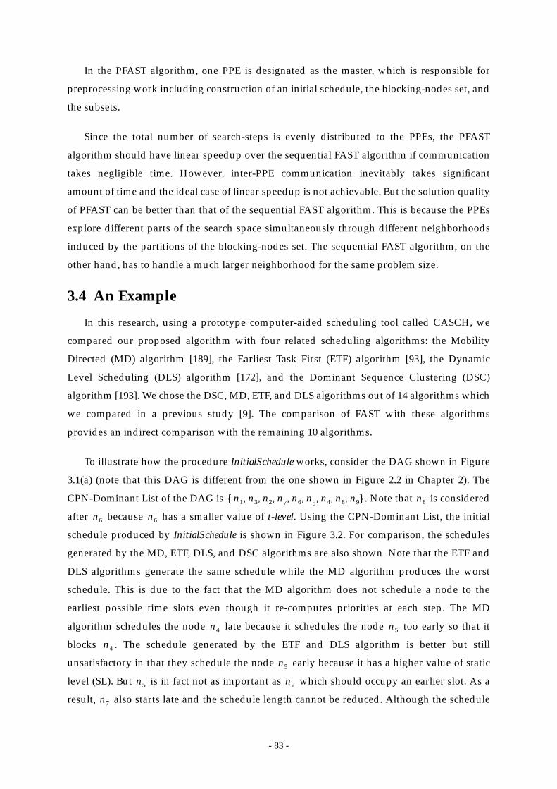
- 83 -

In the PFAST algorithm, one PPE is designated as the master, which is responsible for

preprocessing work including construction of an initial schedule, the blocking-nodes set, and

the subsets.

Since the total number of search-steps is evenly distributed to the PPEs, the PFAST

algorithm should have linear speedup over the sequential FAST algorithm if communication

takes negligible time. However, inter-PPE communication inevitably takes significant

amount of time and the ideal case of linear speedup is not achievable. But the solution quality

of PFAST can be better than that of the sequential FAST algorithm. This is because the PPEs

explore different parts of the search space simultaneously through different neighborhoods

induced by the partitions of the blocking-nodes set. The sequential FAST algorithm, on the

other hand, has to handle a much larger neighborhood for the same problem size.

3.4 An Example

In this research, using a prototype computer-aided scheduling tool called CASCH, we

compared our proposed algorithm with four related scheduling algorithms: the Mobility

Directed (MD) algorithm [189], the Earliest Task First (ETF) algorithm [93], the Dynamic

Level Scheduling (DLS) algorithm [172], and the Dominant Sequence Clustering (DSC)

algorithm [193]. We chose the DSC, MD, ETF, and DLS algorithms out of 14 algorithms which

we compared in a previous study [9]. The comparison of FAST with these algorithms

provides an indirect comparison with the remaining 10 algorithms.

To illustrate how the procedure InitialSchedule works, consider the DAG shown in Figure

3.1(a) (note that this DAG is different from the one shown in Figure 2.2 in Chapter 2). The

CPN-Dominant List of the DAG is . Note that is considered

after because has a smaller value of t-level. Using the CPN-Dominant List, the initial

schedule produced by InitialSchedule is shown in Figure 3.2. For comparison, the schedules

generated by the MD, ETF, DLS, and DSC algorithms are also shown. Note that the ETF and

DLS algorithms generate the same schedule while the MD algorithm produces the worst

schedule. This is due to the fact that the MD algorithm does not schedule a node to the

earliest possible time slots even though it re-computes priorities at each step. The MD

algorithm schedules the node late because it schedules the node too early so that it

blocks . The schedule generated by the ETF and DLS algorithm is better but still

unsatisfactory in that they schedule the node early because it has a higher value of static

level (SL). But is in fact not as important as which should occupy an earlier slot. As a

result, also starts late and the schedule length cannot be reduced. Although the schedule

n1 n3 n2 n, 7 n6 n, 5 n4 n8 n9, , , , , ,{ } n8

n6 n6

n4 n5

n4

n5

n5 n2

n7

- 84 -

generated by the DSC algorithm is slightly better, it has a problem in that the node is

scheduled to a late time slot because its parent is not scheduled to the same processor due

to the minimization of ‘s start-time. The schedule length generated by InitialSchedule is the

shortest, despite its simple scheduling strategy.

To illustrate the effectiveness of the neighborhood search process, consider an initial

schedule shown previously in Figure 3.2(d). The blocking-nodes list of the DAG is

. We can notice that the node blocks the CPN . In the random search

process it is highly probable that is selected for transferring. Suppose it is transferred from

PE 1 to PE 3. The resulting schedule is shown in Figure 3.2(e), from which we can see that

despite the increased start times of and , the final schedule length is nonetheless

shortened.

3.5 Performance Results

In this section we first present the performance results of the sequential FAST algorithm

and compare it with those of DSC, MD, ETF, and DLS algorithms using a prototype

parallelization tool called CASCH. In Section 3.5.4 we present the performance results of the

PFAST algorithm by using two suites of random task graphs for which optimal solutions are

known. In Section 3.5.5 we present the results of applying the algorithm to large DAGs. For

node SL t-level (ASAP) b-level ALAP* 12 0 37 0

8 6 23 148 3 23 149 3 20 1710 3 30 75 10 15 22

* 5 22 15 225 18 15 22

* 1 36 1 36

n1

n2

n3

n4

n5

n6

n7

n8

n9

(a)(b)

Figure 3.1: (a) A task graph; (b) The static levels (SLs), t-levels (ASAP times),b-levels, and ALAP times of the nodes (CPNs are marked by an asterisk).

n1

2

n2

3

n5

5

n9

1

n3

3

n7

4

n4

4

n8

4

n6

4

1

20

1

1

1

14

51

55

10

10

1010

n8

n4

n4

n2 n, 3 n4 n5 n6 n8, , , ,{ } n6 n9

n6

n5 n8

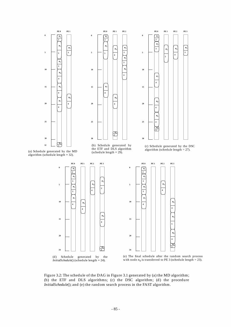
- 85 -

PE 0 PE 1 PE 2 PE 3

PE 0 PE 1 PE 2 PE 3PE 0 PE 1 PE 2PE 0 PE 1

n1

2

n2

3

n5

5

n91

n3

3

n7

4

n4

4

n8

4

n6

4

(b) Schedule generated bythe ETF and DLS algorithm(schedule length = 29).

Figure 3.2: The schedule of the DAG in Figure 3.1 generated by (a) the MD algorithm;(b) the ETF and DLS algorithms; (c) the DSC algorithm; (d) the procedureInitialSchedule(); and (e) the random search process in the FAST algorithm.

n1

2

n2

3

n5

5

n91

n3

3

n7

4

n4

4

0

5

10

15

20

n8

4

n6

4

(a) Schedule generated by the MDalgorithm (schedule length = 32).

0

5

10

15

20

25

30

32

n1

2

n2

3

n5

5

n91

n3

3

n7

4

n4

4

0

5

10

15

20

n8

4

n6

4

25

30

n1

2

n2

3 n5

5

n91

n3

3

n7

4

n4

4

0

5

10

15

20n8

4

n6

425

30

(c) Schedule generated by the DSCalgorithm (schedule length = 27).

24

PE 0 PE 1 PE 2 PE 3

n1

2

n2

3

n5

5

n91

n3

3

n7

4

n4

4

n8

4

n6

4

0

5

10

15

20

24

(d) Schedule generated by theInitialSchedule() (schedule length = 24).

(e) The final schedule after the random search processwith node n6 is transferred to PE 3 (schedule length = 23).

- 86 -

comparison, the results of the DLS, DSC, and ETF algorithms are also shown.

3.5.1 Number of Search Steps

Before comparing the performance of the sequential FAST algorithm with other

algorithms, we performed experiments to determine the constants MAXSTEP and

MAXCOUNT which governs the number of search steps and probabilistic jumps. We

generated 10 random task graphs with 1,000 nodes each (the method of generating these

random graphs is elaborated in Section 3.5.4) and then tested the FAST algorithm with

different values of MAXSTEP and MAXCOUNT. In one set of experiments we varied the

MAXSTEP from 2 to 64 and fixed MAXCOUNT to be 256 which is large enough to isolate its

effect. In the other set of experiments we varied MAXCOUNT from 16 to 256 and fixed

MAXSTEP to be 64. The results of these experiments are shown in Figure 3.3. Each point in

the plots is the average normalized schedule lengths (NSLs) of ten random graphs. The NSL

of a graph is defined as the ratio of the schedule length to the sum of computation costs on

the CP. As can be seen from the plots, the average NSLs did not improve considerably when

we increased MAXSTEP beyond 8 and MAXCOUNT beyond 64. Thus, we fixed MAXSTEP to

be 8 and MAXCOUNT to be 64 throughout the subsequent experiments.

3.5.2 CASCH

We performed experiments using real workload generated from serial applications by a

prototype parallelization and scheduling tool called CASCH (Computer Aided SCHeduling).

The system organization of CASCH is shown in Figure 3.4.

Figure 3.3: Average normalized schedule lengths of the FAST algorithms for randomtask graphs with 1000 nodes with various values of MAXSTEP and MAXCOUNT.

- 87 -

The CASCH tool generates a task graph from a sequential program, uses a scheduling

algorithm to perform scheduling, and then generates the parallel code in a scheduled form

for the Intel Paragon. The timings for the nodes and edges on the DAG are assigned through

a timing database which was obtained through benchmarking. CASCH also provides a

graphical interface to interactively run and test various algorithms including the ones

discussed in this paper. Instead of only measuring the schedule length through a Gantt chart,

we measure the running time of the scheduled code on the Paragon. Various scheduling

algorithms, therefore, can be more accurately tested and compared through CASCH using

real applications on an actual machine. The reader is referred to [10] for details about the tool.

In addition, in order to examine the performance of the algorithm given very large graphs

which can arise in practice, we performed experiments with randomly generated large DAGs

consisting of thousands of nodes.

Figure 3.4: The system organization of CASCH.

PerformanceEvaluation Module

Task GraphsEditing Tools

ArchitectureEditing Tools

Gantt ChartsDisplay

Clusters MapDisplay

Comm. LinksDisplay

ApplicationStatistics

MachineStatistics

SequentialUser Program

Compilation module(Lexer and parser)

Task GraphsGenerator

Scheduling

Mapping

CommunicationsInsertion

Code Generator

X-Windows GUI

PerformanceReports

Task SymbolicInformation Table

ComputationsTimings

CommunicationsTimings

Input/OutputTimings

Weight Estimator

Intel Paragon

Scheduling/MappingAlgorithms Libraries

Clusters ofWorkstations

MappingAlgorithms

MD by Wu & Gajski [189]

DSC by Yang & Gerasoulis [193]

FAST

ETF by Hwang et al. [93]

DLS by Sih and Lee [172]

SchedulingAlgorithms

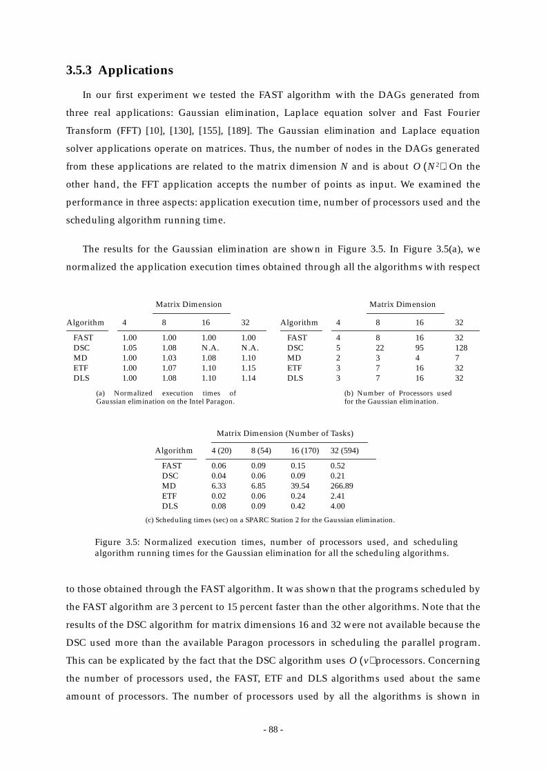
- 88 -

3.5.3 Applications

In our first experiment we tested the FAST algorithm with the DAGs generated from

three real applications: Gaussian elimination, Laplace equation solver and Fast Fourier

Transform (FFT) [10], [130], [155], [189]. The Gaussian elimination and Laplace equation

solver applications operate on matrices. Thus, the number of nodes in the DAGs generated

from these applications are related to the matrix dimension N and is about . On the

other hand, the FFT application accepts the number of points as input. We examined the

performance in three aspects: application execution time, number of processors used and the

scheduling algorithm running time.

The results for the Gaussian elimination are shown in Figure 3.5. In Figure 3.5(a), we

normalized the application execution times obtained through all the algorithms with respect

to those obtained through the FAST algorithm. It was shown that the programs scheduled by

the FAST algorithm are 3 percent to 15 percent faster than the other algorithms. Note that the

results of the DSC algorithm for matrix dimensions 16 and 32 were not available because the

DSC used more than the available Paragon processors in scheduling the parallel program.

This can be explicated by the fact that the DSC algorithm uses processors. Concerning

the number of processors used, the FAST, ETF and DLS algorithms used about the same

amount of processors. The number of processors used by all the algorithms is shown in

O N2( )

FASTDSCMDETFDLS

1.00 1.00 1.00 1.001.05 1.08 N.A. N.A.1.00 1.03 1.08 1.101.00 1.07 1.10 1.151.00 1.08 1.10 1.14

4 8 16 32Algorithm

FASTDSCMDETFDLS

4 8 16 325 22 95 1282 3 4 73 7 16 323 7 16 32

4 8 16 32Algorithm

(a) Normalized execution times ofGaussian elimination on the Intel Paragon.

(b) Number of Processors usedfor the Gaussian elimination.

FASTDSCMDETFDLS

0.06 0.09 0.15 0.520.04 0.06 0.09 0.216.33 6.85 39.54 266.890.02 0.06 0.24 2.410.08 0.09 0.42 4.00

4 (20) 8 (54) 16 (170) 32 (594)Algorithm

Matrix Dimension (Number of Tasks)

(c) Scheduling times (sec) on a SPARC Station 2 for the Gaussian elimination.

Figure 3.5: Normalized execution times, number of processors used, and schedulingalgorithm running times for the Gaussian elimination for all the scheduling algorithms.

Matrix Dimension Matrix Dimension

O v( )

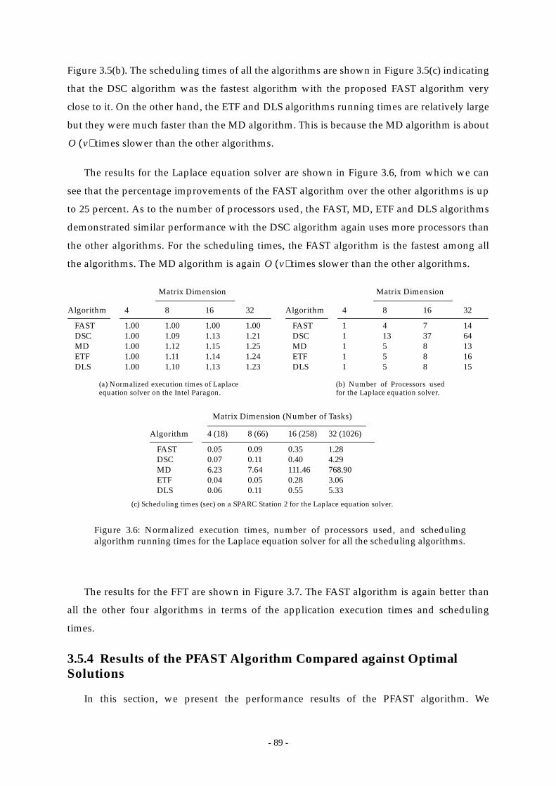
- 89 -

Figure 3.5(b). The scheduling times of all the algorithms are shown in Figure 3.5(c) indicating

that the DSC algorithm was the fastest algorithm with the proposed FAST algorithm very

close to it. On the other hand, the ETF and DLS algorithms running times are relatively large

but they were much faster than the MD algorithm. This is because the MD algorithm is about

times slower than the other algorithms.

The results for the Laplace equation solver are shown in Figure 3.6, from which we can

see that the percentage improvements of the FAST algorithm over the other algorithms is up

to 25 percent. As to the number of processors used, the FAST, MD, ETF and DLS algorithms

demonstrated similar performance with the DSC algorithm again uses more processors than

the other algorithms. For the scheduling times, the FAST algorithm is the fastest among all

the algorithms. The MD algorithm is again times slower than the other algorithms.

The results for the FFT are shown in Figure 3.7. The FAST algorithm is again better than

all the other four algorithms in terms of the application execution times and scheduling

times.

3.5.4 Results of the PFAST Algorithm Compared against OptimalSolutions

In this section, we present the performance results of the PFAST algorithm. We

O v( )

O v( )

FASTDSCMDETFDLS

1.00 1.00 1.00 1.001.00 1.09 1.13 1.211.00 1.12 1.15 1.251.00 1.11 1.14 1.241.00 1.10 1.13 1.23

4 8 16 32Algorithm

FASTDSCMDETFDLS

1 4 7 141 13 37 641 5 8 131 5 8 161 5 8 15

4 8 16 32Algorithm

(b) Number of Processors usedfor the Laplace equation solver.

FASTDSCMDETFDLS

0.05 0.09 0.35 1.280.07 0.11 0.40 4.296.23 7.64 111.46 768.900.04 0.05 0.28 3.060.06 0.11 0.55 5.33

4 (18) 8 (66) 16 (258) 32 (1026)Algorithm

Matrix Dimension (Number of Tasks)

(c) Scheduling times (sec) on a SPARC Station 2 for the Laplace equation solver.

Matrix Dimension Matrix Dimension

(a) Normalized execution times of Laplaceequation solver on the Intel Paragon.

Figure 3.6: Normalized execution times, number of processors used, and schedulingalgorithm running times for the Laplace equation solver for all the scheduling algorithms.

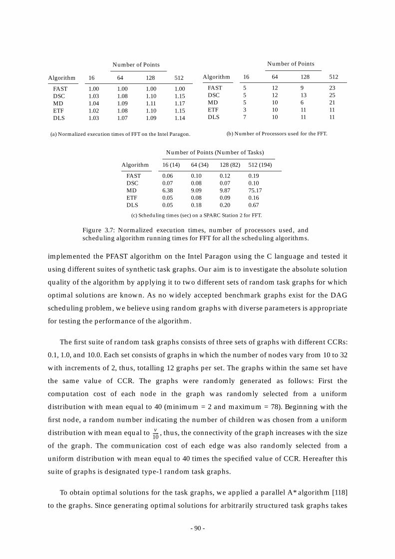
- 90 -

implemented the PFAST algorithm on the Intel Paragon using the C language and tested it

using different suites of synthetic task graphs. Our aim is to investigate the absolute solution

quality of the algorithm by applying it to two different sets of random task graphs for which

optimal solutions are known. As no widely accepted benchmark graphs exist for the DAG

scheduling problem, we believe using random graphs with diverse parameters is appropriate

for testing the performance of the algorithm.

The first suite of random task graphs consists of three sets of graphs with different CCRs:

0.1, 1.0, and 10.0. Each set consists of graphs in which the number of nodes vary from 10 to 32

with increments of 2, thus, totalling 12 graphs per set. The graphs within the same set have

the same value of CCR. The graphs were randomly generated as follows: First the

computation cost of each node in the graph was randomly selected from a uniform

distribution with mean equal to 40 (minimum = 2 and maximum = 78). Beginning with the

first node, a random number indicating the number of children was chosen from a uniform

distribution with mean equal to , thus, the connectivity of the graph increases with the size

of the graph. The communication cost of each edge was also randomly selected from a

uniform distribution with mean equal to 40 times the specified value of CCR. Hereafter this

suite of graphs is designated type-1 random task graphs.

To obtain optimal solutions for the task graphs, we applied a parallel A* algorithm [118]

to the graphs. Since generating optimal solutions for arbitrarily structured task graphs takes

FASTDSCMDETFDLS

1.00 1.00 1.00 1.001.03 1.08 1.10 1.151.04 1.09 1.11 1.171.02 1.08 1.10 1.151.03 1.07 1.09 1.14

16 64 128 512Algorithm

FASTDSCMDETFDLS

5 12 9 235 12 13 255 10 6 213 10 11 117 10 11 11

16 64 128 512Algorithm

(b) Number of Processors used for the FFT.

FASTDSCMDETFDLS

0.06 0.10 0.12 0.190.07 0.08 0.07 0.106.38 9.09 9.87 75.170.05 0.08 0.09 0.160.05 0.18 0.20 0.67

16 (14) 64 (34) 128 (82) 512 (194)Algorithm

Number of Points (Number of Tasks)

(c) Scheduling times (sec) on a SPARC Station 2 for FFT.

Number of Points Number of Points

Figure 3.7: Normalized execution times, number of processors used, andscheduling algorithm running times for FFT for all the scheduling algorithms.

(a) Normalized execution times of FFT on the Intel Paragon.

v10------

- 91 -

exponential time, it is not feasible to obtain optimal solutions for large graphs. On the other

hand, to investigate the scalability of the PFAST algorithm, it is desirable to test it with larger

task graphs for which optimal solutions are known. To resolve this problem, we employed a

different strategy to generate the second suite of random task graphs. Rather than trying to

find out the optimal solutions after the graphs are randomly generated, we set out to

generate task graphs with given optimal schedule lengths and number of processors used in

the optimal schedules.

The method of generating task graphs with known optimal schedules is as follows:

Suppose that the optimal schedule length of a graph and the number of processors used are

specified as and p, respectively. For each PE i, we randomly generate a number from

a uniform distribution with mean . The time interval between 0 and of PE i is then

randomly partitioned into sections. Each section represents the execution span of one task,

thus, tasks are “scheduled” to PE i with no idle time slot. In this manner, v tasks are

generated so that every processor has the same schedule length. To generate an edge, two

tasks and are randomly chosen such that . The edge is made to

emerge from to . As to the edge weight, there are two cases to consider: (i) the two tasks

are scheduled to different processors, and (ii) the two tasks are scheduled to the same

processor. In the first case the edge weight is randomly chosen from a uniform distribution

with maximum equal to (the mean is adjusted according to the given

CCR value). In the second case the edge weight can be an arbitrary positive integer because

the edge does not affect the start and finish times of the tasks which are scheduled to the same

processor. We randomly chose the edge weight for this case according to the given CCR

value. Using this method, we generated three sets of task graphs with three CCRs: 0.1, 1.0,

and 10.0. Each set consists of graphs in which the number of nodes vary from 50 to 500 in

increments of 50; thus, each set contains 10 graphs. The graphs within the same set have the

same value of CCR. Hereafter we call this suite of graphs the type-2 random task graphs.

Table 3.1 shows the results of the PFAST algorithm using 1, 2, 4, 8, and 16 PPEs on the

Intel Paragon. Using 1 PPE means that the algorithm is the sequential FAST algorithm. It

should be noted that for graphs of smaller size, the blocking-nodes subsets of the PPEs are

not disjoint so as to make each subset contain at least 2 nodes. In the table, the total number of

optimal solutions generated and the average percentage deviations (from the optimal

solutions) for each CCR are also shown. Note that the average percentage deviations are

calculated by dividing the total deviations by the number of non-optimal cases only. These

average deviations thus indicate more accurately the performance of the PFAST algorithm

SLopt xi

vp--- SLopt

xi

xi

na nb FT na( ) ST nb( )<

na nb

ST nb( ) FT na( )–( )

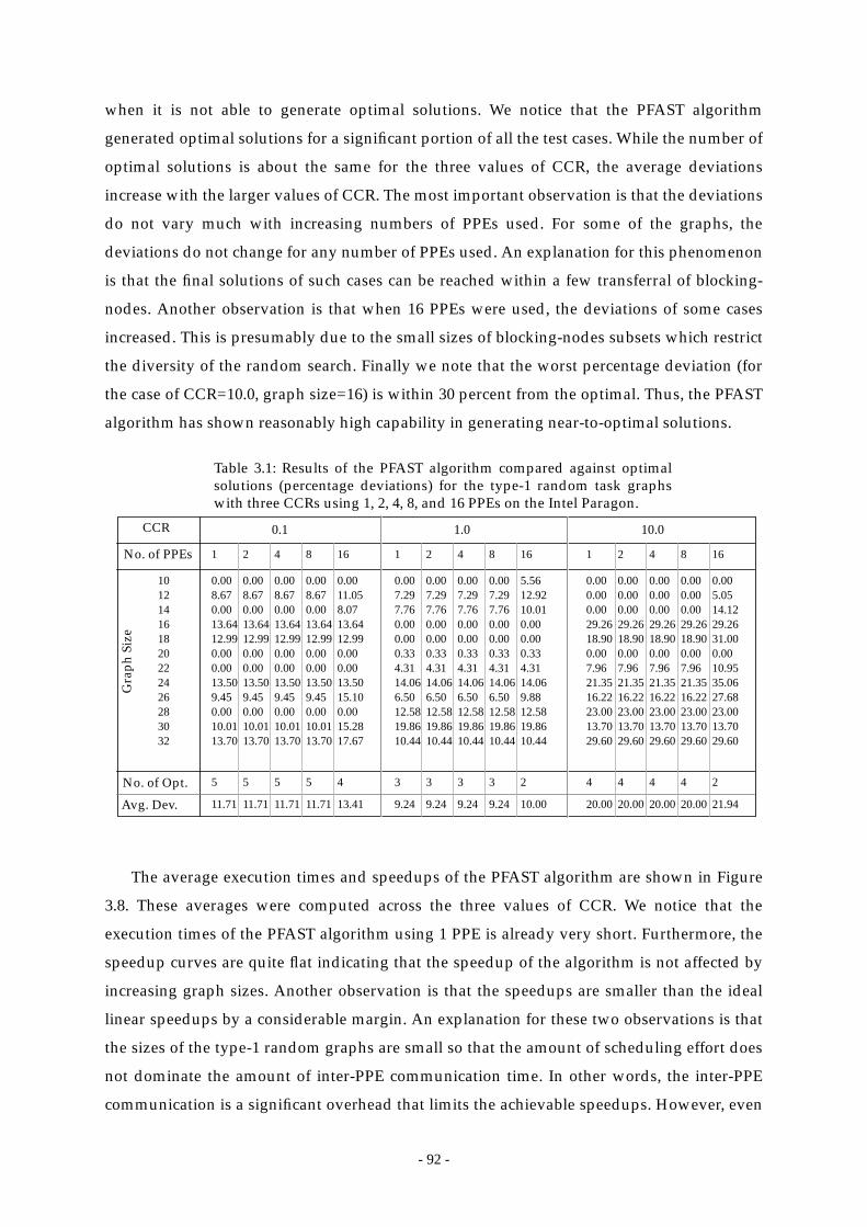
- 92 -

when it is not able to generate optimal solutions. We notice that the PFAST algorithm

generated optimal solutions for a significant portion of all the test cases. While the number of

optimal solutions is about the same for the three values of CCR, the average deviations

increase with the larger values of CCR. The most important observation is that the deviations

do not vary much with increasing numbers of PPEs used. For some of the graphs, the

deviations do not change for any number of PPEs used. An explanation for this phenomenon

is that the final solutions of such cases can be reached within a few transferral of blocking-

nodes. Another observation is that when 16 PPEs were used, the deviations of some cases

increased. This is presumably due to the small sizes of blocking-nodes subsets which restrict

the diversity of the random search. Finally we note that the worst percentage deviation (for

the case of CCR=10.0, graph size=16) is within 30 percent from the optimal. Thus, the PFAST

algorithm has shown reasonably high capability in generating near-to-optimal solutions.

The average execution times and speedups of the PFAST algorithm are shown in Figure

3.8. These averages were computed across the three values of CCR. We notice that the

execution times of the PFAST algorithm using 1 PPE is already very short. Furthermore, the

speedup curves are quite flat indicating that the speedup of the algorithm is not affected by

increasing graph sizes. Another observation is that the speedups are smaller than the ideal

linear speedups by a considerable margin. An explanation for these two observations is that

the sizes of the type-1 random graphs are small so that the amount of scheduling effort does

not dominate the amount of inter-PPE communication time. In other words, the inter-PPE

communication is a significant overhead that limits the achievable speedups. However, even

101214161820222426283032

Gra

ph S

ize

No. of Opt.

Avg. Dev.

Table 3.1: Results of the PFAST algorithm compared against optimalsolutions (percentage deviations) for the type-1 random task graphswith three CCRs using 1, 2, 4, 8, and 16 PPEs on the Intel Paragon.

CCR

No. of PPEs

0.00 0.00 0.00 0.00 0.000.00 0.00 0.00 0.00 5.050.00 0.00 0.00 0.00 14.1229.26 29.26 29.26 29.26 29.2618.90 18.90 18.90 18.90 31.000.00 0.00 0.00 0.00 0.007.96 7.96 7.96 7.96 10.9521.35 21.35 21.35 21.35 35.0616.22 16.22 16.22 16.22 27.6823.00 23.00 23.00 23.00 23.0013.70 13.70 13.70 13.70 13.7029.60 29.60 29.60 29.60 29.60

1 2 4 8 16

10.0

4 4 4 4 2

20.00 20.00 20.00 20.00 21.94

0.00 0.00 0.00 0.00 5.567.29 7.29 7.29 7.29 12.927.76 7.76 7.76 7.76 10.010.00 0.00 0.00 0.00 0.000.00 0.00 0.00 0.00 0.000.33 0.33 0.33 0.33 0.334.31 4.31 4.31 4.31 4.3114.06 14.06 14.06 14.06 14.066.50 6.50 6.50 6.50 9.8812.58 12.58 12.58 12.58 12.5819.86 19.86 19.86 19.86 19.8610.44 10.44 10.44 10.44 10.44

1 2 4 8 16

1.0

3 3 3 3 2

9.24 9.24 9.24 9.24 10.00

0.00 0.00 0.00 0.00 0.008.67 8.67 8.67 8.67 11.050.00 0.00 0.00 0.00 8.0713.64 13.64 13.64 13.64 13.6412.99 12.99 12.99 12.99 12.990.00 0.00 0.00 0.00 0.000.00 0.00 0.00 0.00 0.0013.50 13.50 13.50 13.50 13.509.45 9.45 9.45 9.45 15.100.00 0.00 0.00 0.00 0.0010.01 10.01 10.01 10.01 15.2813.70 13.70 13.70 13.70 17.67

1 2 4 8 16

0.1

5 5 5 5 4

11.71 11.71 11.71 11.71 13.41

- 93 -

for such small graphs, the PFAST algorithm exhibited reasonable scalability.

Table 3.2 shows the results of the PFAST algorithm for the type-2 random task graphs

using 1, 2, 4, 8, and 16 PPEs on the Intel Paragon. For these much larger graphs, the PFAST

algorithm generated only one optimal solution (the case of CCR = 0.1, size = 50). However, an

encouraging observation is that the percentage deviations are small. Indeed, the best

deviation is only 2.43 percent and the worst only 45.01 percent, which can be considered as

close-to-optimal. The average deviations, which increase with increasing CCR, are smaller

than 30 percent. A very interesting observation is that for some cases of larger task graphs

(e.g., sizes larger than 200), using more PPEs improve the schedule lengths. For example, in

the case of CCR = 0.1 and size = 300, using 4 PPEs resulted in a deviation of 18.79 percent

while using 8 PPEs gave a deviation of 16.56 percent. Using 16 PPEs further decreased the

deviation to 14.27 percent. This observation implies that parallelization of a search algorithm

can potentially improve the solution quality. This is due to the partitioning of the search

neighborhood which lets the search to explore different regions of the search space

simultaneously, thereby increasing the likelihood of getting better solutions. There are a few

cases in which using more PPEs resulted in an increased deviations, however. For example,

for the case of CCR = 10.0 and size = 250, using 4 PPEs gave a deviation of 34.06 percent,

while using 8 PPEs improved the deviation to 25.67 percent. However, when 16 PPEs were

used, the deviation was only 29.43 percent, which is worse than that of using 8 PPEs but

better than that of using 4 PPEs.

The average execution times and speedups of the PFAST algorithm for the type-2 random

task graphs are shown in Figure 3.9. Compared with the speedup plots shown earlier in

50 100 150 200 250 300 350 400 450 5000

2

4

6

8

10

12

2 PPEs4 PPEs8 PPEs16 PPEs

Figure 3.8: (a) The average running times of the PFAST algorithm for the type-1 random task graphs with three CCRs using 1 PPE on the Intel Paragon; (b)the average speedups of the PFAST algorithm for 2, 4, 8, and 16 PPEs.

(a) Average running times using 1 PPE.

(b) Average speedups.

101214161820222426283032

Graph Size

0.0600.0610.0630.0660.0730.0760.0780.0790.0830.0870.0950.098

Running Times (secs)

- 94 -

Figure 3.8, the speedups for type-2 task graphs are considerably higher. This is because inter-

PPE communication for larger task graphs is not a significant overhead. Again the PFAST

demonstrated reasonably good scalability even for task graphs with 500 nodes.

Based on the above results we can conclude that the PFAST algorithm is suitable for

finding high quality schedules for large task graphs under strict running times requirements.

3.5.5 Large DAGs

To test the scalability and robustness of the FAST algorithm we performed experiments

with very large DAGs. These DAGs include a 10728-node Gaussian elimination graph, a

50100150200250300350400450500

Gra

ph S

ize

No. of Opt.

Avg. Dev.

Table 3.2: Results of the PFAST algorithm compared against optimalsolutions (percentage deviations) for the type-2 random task graphswith three CCRs using 1, 2, 4, 8, and 16 PPEs on the Intel Paragon.

CCR

No. of PPEs

29.26 29.26 29.26 29.26 29.2645.01 45.01 45.01 45.01 45.0117.13 17.13 17.13 17.13 17.1320.34 20.34 20.34 15.28 13.5734.06 34.06 34.06 25.67 29.4322.93 22.93 22.93 15.84 14.4538.94 38.94 38.94 33.86 22.5326.58 26.58 26.58 18.79 14.3133.95 33.95 33.95 24.65 19.4635.97 35.97 35.97 32.66 31.65

1 2 4 8 16

10.0

0 0 0 0 0

25.35 25.35 25.35 21.51 19.23

5.34 5.34 5.34 5.34 5.3414.90 14.90 14.90 14.90 14.9016.83 16.83 16.83 16.83 16.8319.02 19.02 19.02 18.08 16.0726.97 26.97 26.97 25.99 22.1125.30 25.30 25.30 23.28 20.1225.11 25.11 25.11 25.01 24.6215.03 15.03 15.03 13.37 11.6426.38 26.38 26.38 25.53 26.3830.71 30.71 30.71 29.31 25.98

1 2 4 8 16

1.0

0 0 0 0 0

17.13 17.13 17.13 16.47 14.98

0.00 0.00 0.00 0.00 0.005.57 5.57 5.57 5.57 5.5717.80 17.80 17.80 17.80 17.8013.69 13.69 13.69 13.69 13.692.83 2.83 2.83 2.83 2.4318.79 18.79 18.79 16.56 14.2717.20 17.20 17.20 15.12 14.7816.20 16.20 16.20 14.43 14.207.04 7.04 7.04 6.22 5.4616.33 16.33 16.33 13.92 14.18

1 2 4 8 16

0.1

1 1 1 1 1

10.50 10.50 10.50 9.65 9.22

50 100 150 200 250 300 350 400 450 5000

2

4

6

8

10

12

14

16


Figure 3.9: (a) The average running times of the PFAST algorithm for the type-2random task graphs with three CCRs using 1 PPE on the Intel Paragon; (b) theaverage speedups of the PFAST algorithm for 2, 4, 8, and 16 PPEs.



50100150200250300350400450500

Graph Size

0.1240.4950.9871.8342.9834.4335.9857.1239.15111.238


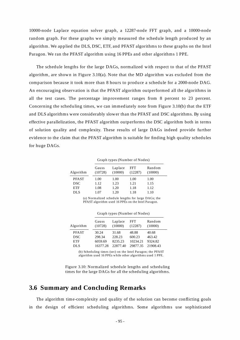
- 95 -

10000-node Laplace equation solver graph, a 12287-node FFT graph, and a 10000-node

random graph. For these graphs we simply measured the schedule length produced by an

algorithm. We applied the DLS, DSC, ETF, and PFAST algorithms to these graphs on the Intel

Paragon. We ran the PFAST algorithm using 16 PPEs and other algorithms 1 PPE.

The schedule lengths for the large DAGs, normalized with respect to that of the PFAST

algorithm, are shown in Figure 3.10(a). Note that the MD algorithm was excluded from the

comparison because it took more than 8 hours to produce a schedule for a 2000-node DAG.

An encouraging observation is that the PFAST algorithm outperformed all the algorithms in

all the test cases. The percentage improvement ranges from 8 percent to 23 percent.

Concerning the scheduling times, we can immediately note from Figure 3.10(b) that the ETF

and DLS algorithms were considerably slower than the PFAST and DSC algorithms. By using

effective parallelization, the PFAST algorithm outperforms the DSC algorithm both in terms

of solution quality and complexity. These results of large DAGs indeed provide further

evidence to the claim that the PFAST algorithm is suitable for finding high quality schedules

for huge DAGs.


The algorithm time-complexity and quality of the solution can become conflicting goals

in the design of efficient scheduling algorithms. Some algorithms use sophisticated

(a) Normalized schedule lengths for large DAGs; thePFAST algorithm used 16 PPEs on the Intel Paragon.

(b) Scheduling times (sec) on the Intel Paragon; the PFASTalgorithm used 16 PPEs while other algorithms used 1 PPE.

Figure 3.10: Normalized schedule lengths and schedulingtimes for the large DAGs for all the scheduling algorithms.

PFASTDSCETFDLS

1.00 1.00 1.00 1.001.12 1.23 1.21 1.151.08 1.20 1.18 1.121.07 1.20 1.18 1.10

Gauss Laplace FFT Random(10728) (10000) (12287) (10000)Algorithm

Graph types (Number of Nodes)

PFASTDSCETFDLS

30.24 31.68 48.88 40.68298.34 228.23 600.23 463.426059.69 8235.23 10234.21 9324.8216377.28 22877.40 29877.35 21908.43

Gauss Laplace FFT Random(10728) (10000) (12287) (10000)Algorithm

Graph types (Number of Nodes)

- 96 -

techniques to dynamically track the most important nodes for scheduling. Such algorithms

inevitably have high time-complexity and are inapplicable in practice. Another problem of

the sophisticated algorithms is that they spend great computational effort to optimize the

scheduling of individual nodes, which may or may not result in an optimal schedule. On the

other hand, other low complexity algorithms, whose design goal is to minimize running

times, usually cannot produce high quality solutions. The major problem for such algorithms

is that they use a simple list scheduling method which can hardly be suitable for a wide range

of graph structures. Indeed, our study indicates that not only does the quality of existing

algorithms differ considerably but their running times can vary by even huge margins.

In this chapter we proposed a low complexity algorithm, called the FAST algorithm, to

meet the conflicting goals of high performance and low time-complexity. Instead of using

sophisticated methods to optimize the scheduling of individual nodes, the FAST algorithm

first generates an initial schedule and then refines it using probabilistic search techniques.

The initial schedule is generated by using list scheduling, based on the CPN-Dominant List.

In the CPN-Dominant List, the nodes of the CP occupy earlier positions so that they can be

scheduled to earlier time slots. Given such already-optimized initial schedule, a

neighborhood search method is applied to further shorten the schedule length. In the

neighborhood search, a node is randomly selected from the blocking-node set for transferral

from its original PE to a new PE. The blocking-node set is composed of IBNs and OBNs,

which are relatively unimportant nodes but capable of blocking the CPNs from starting

earlier. If the transferral results in shorter schedule length, it is accepted and the search starts

again in a new neighborhood, otherwise another node is randomly selected.

The proposed FAST scheduling algorithm takes linear-time to generate solutions with

high quality. We have compared the algorithm with a number of well-known efficient

scheduling algorithms using real applications in a prototype automatic parallelization and

scheduling tool called CASCH. The results obtained demonstrate that the proposed

algorithm is superior to existing algorithms in terms of both solution quality and complexity.

The major strength of the algorithm is the construction of the CPN-Dominant list in which

the priorities of tasks are accurately captured. There can be cases in which the initial schedule

is not of a high quality so that the random search process may get stuck in a poor locally

optimal point in the solution space, though. Based on the comparison study in this chapter

and the comparison of 14 algorithms in [10], we find the FAST algorithm to be the fastest

algorithm known to us.

We have also parallelized the FAST algorithm to further reduce its running times. The

- 97 -

parallelization is based on partitioning of the blocking-nodes set. Each subset is distributed to

a distinct PPE in the system in which the algorithm is executed. Using random task graphs

for which optimal solutions are known, the parallelized FAST algorithm, called the PFAST

algorithm, generated optimal solutions for a significant portion of all the test cases, and close-

to-optimal solutions for the remaining cases. The PFAST algorithm also exhibited good

scalability in that it gave consistent performance even when applied to large task graphs. An

interesting observation of the PFAST algorithm is that parallelization can sometimes improve

solution quality in that for some cases the PFAST algorithm generated better solutions when

using more PPEs. This is due to the partitioning of the blocking-nodes set, which implies a

partitioning of the search neighborhood. The partitioning causes the algorithm to explore the

search space simultaneously, thereby enhancing the likelihood of getting better solutions.

The PFAST algorithm is suitable for obtaining high quality solutions under strict running

time requirements. Furthermore, the algorithm is scalable to large input. However, perhaps

the algorithm can be improved using certain low time-complexity algorithmic techniques to

track the actual blocking-nodes set dynamically.

- 98 -

Chapter 4

Scheduling using Parallel Genetic Search

4.1 Introduction

Recently, genetic algorithms (GAs) [45], [73], [87] have been widely reckoned as a useful

vehicle for obtaining high quality solutions or even optimal solutions for a broad range of

combinatorial optimization problems including the scheduling problem [21], [46], [163], the

graph partitioning problem [32], and robotic control problem [69]. While a few GAs for

scheduling have already been suggested, in this chapter we propose a GA-based BNP

scheduling algorithm with the combined objectives of high performance, scalability, and fast

running time. The proposed Parallel Genetic Scheduling (PGS) algorithm itself is a parallel

algorithm which generates high quality solutions in an extremely short time. By encoding

scheduling lists as chromosomes, the PGS algorithm can potentially generate an optimal

scheduling list which in turn leads to an optimal schedule. The major strength of the PGS

algorithm lies in its two efficient genetic operators: the order crossover and mutation. These

operators effectively combine the building-blocks of good scheduling lists to construct better

lists. The proposed algorithm, when evaluated through a robust comparison with the best

known heuristics, outperformed the heuristics in terms of performance and time-complexity,

while taking considerably less running time. When evaluated with random task graphs for

which optimal solutions are known, the algorithm generated optimal solutions for more than

half of the test cases and close-to-optimal for the remaining cases.

As the general scheduling problem is NP-complete, state-space search techniques are

commonly considered to be the only resort for finding optimal solutions [100], [156].

However, most of these techniques, which incur an exponential time in the worst case and

are still designed to work under restricted environments, are usually not applicable to

general situations.

In view of the ineffectiveness of state-space search techniques, our aim is at designing a

new scheduling scheme which not only has a high capability to generate optimal solutions

- 99 -

but is also fast and scalable. To obtain high quality solutions, we devised a genetic

formulation of the scheduling problem in which scheduling lists (ordering of tasks for

scheduling) are systematically combined using computationally efficient operators so as to

determine an optimal scheduling list. To achieve a low time-complexity, the proposed

algorithm is parallelized. The algorithm scales well with the number of processors. Moreover,

the algorithm can handle general DAGs without making simplifying assumptions.

Inspired by the Darwinian concept of evolution, genetic algorithms [45], [56], [73], [87],

[176] are global search techniques which explore different regions of the search space

simultaneously by keeping track of a set of potential solutions called a population. According

to the Building-block Hypothesis [73] and the Schema Theorem [73], a genetic algorithm

systematically combines the good building-blocks of selected individuals in the population

to generate better individuals for survival in the next generation by employing genetic

operators such as crossover and mutation. Another attractive merit of genetic search is that

the parallelization of the algorithm is possible. With these distinctive algorithmic merits,

genetic algorithms are becoming more widely used in many areas to tackle the quest for

optimal solutions in optimization problems. Indeed genetic algorithms have been applied to

the data partitioning problem [45], the graph partitioning problem [32], the robotic control

problem [69], etc.

We formulate the scheduling problem in a genetic search framework based on the

observation that if the tasks of a parallel program are arranged properly in a list, an optimal

schedule may be obtained by scheduling the tasks one by one according to their order in the

list. With this concept, we encode each chromosome to a valid scheduling list, one in which

the precedence constraints among tasks are not violated. We also design two genetic

operators: the order crossover and mutation. These operators effectively combine the good

features of existing scheduling lists to form better lists. Using random task graphs for which

optimal schedules are known, we have found that the proposed algorithm can generate

optimal solutions for a majority of the test cases. Furthermore, when compared with two

efficient scheduling heuristics, the proposed algorithm outperformed them both while taking

much less computation time.

The remainder of this chapter is organized as follow. In the next section we provide the

problem statement. In Section 4.2 we give a background of genetic search by presenting a

brief survey of genetic techniques. In Section 4.3 we present the proposed parallel genetic

scheduling algorithm. Examples are used to illustrate the functionality of the proposed

technique. In Section 4.4 we describe our experimental study and its results. We also describe

- 100 -

some related work on using genetic algorithms for scheduling in Section 4.5. Finally, we

provide some concluding remarks and future research directions in the last section.

4.2 Overview of Genetic Search Techniques

In this section we present a brief review of standard genetic algorithms (SGA), followed

by a discussion of different models of parallel genetic algorithms (PGA).

4.2.1 Standard Genetic Algorithms

Genetic algorithms (GAs), introduced by Holland in the 1970’s [87], are search techniques

that are designed based on the concept of evolution [17], [45], [56], [73], [176]. In simple

terms, given a well-defined search space in which each point is represented by a bit string

called a chromosome, a GA is applied with its three genetic search operators—selection,

crossover, and mutation—with the objective of improving the quality of the chromosomes. A

GA is usually employed to determine the optimal solution of a specific objective function.

The search space, therefore, is defined as the solution space so that each feasible solution is

represented by a distinct chromosome. Before the search starts, a set of chromosomes is

randomly chosen from the search space to form the initial population. The three genetic

search operations are then applied one after the other to obtain a new generation of

chromosomes in which the expected quality over all the chromosomes is better than that of

the previous generation. This process is repeated until the stopping criterion is met and the

best chromosome of the last generation is reported as the final solution. An outline of a

generic GA is as follows. The mechanism of the three operators are discussed in detail in

Section 4.2.2.

Standard Genetic Algorithm (SGA):(1) Generate initial population;(2) while number of generations not exhausted do(3) for i = 1 to PopulationSize do(4) Randomly select two chromosomes and apply the crossover operator;(5) Randomly select one chromosome and apply mutation operator;(6) endfor(7) Evaluate all the chromosomes in the population and perform selection;(8) endwhile(9) Report the best chromosome as the final solution.

In nature we observe that stronger individuals survive, reproduce, and hence transmit

their good characteristics to subsequent generations. This natural selection process inspires

the design of the selection operator in the GAs. Given a generation of chromosomes, each of

- 101 -

them is evaluated by measuring its fitness which, in fact, is the quality of the solution the

chromosome represents. The fitness value is usually normalized to a real number between 0

and 1, and the higher the value, the fitter the chromosome. Usually a proportionate selection

scheme is used. With this scheme, a chromosome with a fitness value is allocated

offspring in the subsequent generation, where is the average fitness value of the

population. Thus, a chromosome with a larger fitness value is allocated more offsprings

while a chromosome with a smaller fitness value, for example, less than the average, may be

discarded in the next generation.

GAs are least affected by the continuity properties of the search space unlike many other

heuristic approaches. Many researchers have found that GAs are better than simulated

annealing [144] as well as tabu search [71], [72], both of which operate on one single solution

only.

For an efficient GA search, in addition to a proper solution structure, it is necessary that

the initial population of solutions be a diverse representative of the search space.

Furthermore, the solution encoding should permit:

• a large diversity in a small population;• easy crossover and mutation operations;• an easy computation of the objective function.

4.2.2 Genetic Search Operators

In this section we review the mechanism and characteristics of three commonly used

standard genetic operators: crossover, mutation, and inversion.

Crossover is a crucial operator of a GA and is applied after selection. While selection is

used to improve the overall quality of the population, crossover is used to explore the search

space to find better individuals. Pairs of chromosomes are selected randomly from the

population for application of the crossover operator. In the simplest approach a point is

chosen randomly as the crossover point. The two chromosomes exchange the portions of the

strings beyond the crossover point to generate two new chromosomes. A simple example of

the standard crossover is given in Figure 4.1(a). The rationale is that after the exchange the

newly generated chromosomes may contain the good characteristics from both the parent

chromosomes, and hence possess a higher fitness value. Nevertheless, the newly generated

chromosomes may be worse than their parents. With respect to this, the crossover operator is

not always applied to the selected pair of chromosomes. Instead, it is applied with a certain

pre-specified probability called the crossover rate, denoted by . There are a number of

f f favg⁄

favg

µc

- 102 -

variants of the standard crossover operators. These include order crossover, partially-mapped

crossover (PMX), and cycle crossover [73]. The characteristics of these variants will be described

later in this chapter.

Mutation is a genetic operator for recovering the good characteristics lost during

crossover. Mutation of a chromosome is achieved by simply flipping a randomly selected bit

of the chromosome. A simple example of the standard mutation is given in Figure 4.1(b). Like

a crossover, mutation is applied with a certain probability called the mutation rate, which is

denoted by . Although mutation is a secondary search operator, it is useful for escaping

from local minima. For instance, suppose all the chromosomes have converged to 0 at a

certain bit position while the optimal solution has a 1 at that position. Crossover cannot

regenerate a 1 at that position but a mutation may be able to. If we only use crossover, the

pattern diversity, which corresponds to the breadth of the search domain, will inevitably be

limited.

An inversion operator takes a random segment in a chromosome and reverses it. A

simple example of the standard inversion is given in Figure 4.1(c). The advantage of the

inversion operator is as follows. There are groups of properties or genes which would be

advantageous for offsprings to inherit from one parent. Such groups of genes, which interact

to increase the fitness of the offspring which inherit them are said to be co-adapted. If two

genes are close to each other in the chromosome, the probability of being split up when the

1 0 1 0 1 0 1 0

1 0 0 0 0 1 1 1

crossover point

Parent 1 (Target Parent)

Parent 2 (Passing Parent)

1 0 1 0 1 1 1 1

(a) Standard crossover.

1 0 1 0 1 1 1 1 1 0 1 0 1 1 0 1Mutated the 7th bit

(b) Standard mutation.

1 0 1 0 1 1 1 1 1 0 1 1 1 1 0 1

Segment to be inverted

Inversion

(c) Standard inversion.

Figure 4.1: Examples of the standard (a) crossover operator; (b) mutationoperator; and (c) inversion operator on a binary coded chromosome.

µm

- 103 -

crossover operator divides the chromosome into two segments will be less.

4.2.3 Control Parameters

A GA is governed by a number of parameters including population size , number of

generations , crossover rate and mutation rate . Finding appropriate values of these

parameters requires extensive experimentations [45], [58], [73]. Even with appropriate

parameters, optimal solutions cannot be guaranteed due to the probabilistic nature of GAs.

Grefenstette [79] proposed using the scaling method for preventing a premature convergence, a

scenario in which chromosomes of a population become homogeneous and converge to a

sub-optimal chromosome. Scaling involves re-adjusting the fitness values of solutions in

order to sustain a steady selective pressure in the population so that a premature

convergence may be avoided. Srinivas and Patnaik [175] proposed an adaptive method to

tune parameters on the fly based on the idea of sustaining diversity in a population without

affecting its convergence properties. Their algorithm protects the best solutions in each

generation from being disrupted by crossover and mutation. Extensive experiments have

shown that such adaptive strategy can help prevent a GA from getting stuck at local minima.

4.2.4 Parallel Genetic Algorithms

The inherent parallelism in GAs can be exploited to enhance their search efficiency. In

contrast to simulated annealing which is intrinsically sequential and thus hard to parallelize

[144], parallelism in GAs is easier to exploit [76], [80], [91], [98], [124], [141], [142], [143], [180],

[181]. One of the approaches of parallelizing a GA is to divide the population into q

partitions, where q is the number of physical processing elements (PPEs) on which the parallel

GA is executed. Each subpopulation in a PPE contains more than one chromosome, and each

PPE runs a separate copy of the original GA with its own partition of the population. Such a

parallel GA (PGA) is called the coarse-grained GA. Two less common types of PGAs are the

fine-grained GA and the micro-grained GA. In a fine-grained GA exactly one chromosome is

assigned to each PPE. In this type of PGA, it is the topology of the PPE network that

determines the degree of population isolation, and hence diversity, of the individuals in the

whole population. In a micro-grained GA, a single population is maintained across all PPEs,

and parallelism comes from the use of multiple PPEs to evaluate the individual fitness

function. We employ the coarse-grained parallelization approach.

In a coarse-grained PGA, there are many possible schemes for the PPEs to communicate

and exchange information about solutions [98], [124], [141], [142]. The objective of

communication is to transfer fitter chromosomes from their local populations to other PPEs

Np

Ng µc µm

- 104 -

for parallel exploitation. There are two major models of communication: the isolated island

model and the connected island model.

In an isolated island model, PPEs work totally independently and communicate only at

the end of the search process to select the best solution among all the PPEs. Since no

migration of fitter chromosomes is performed, linear speedup can be achieved. However, a

PPE may waste all its processing cycles when it gets stuck at a poor population without

knowing that other PPEs are searching in more promising regions in the search space. This in

turn is a result of partitioning the population, which reduces the diversity of the

chromosomes in the search space.

In a connected island model, PPEs communicate periodically to exchange information

concerning their solutions found [159]. It is common for the best chromosome found to be

broadcast to all PPEs so that every PPE may devote processing power towards the most

promising direction. There are two variants of the connected island model. The first is that

PPEs communicate in a synchronous fashion, that is, all PPEs participate in a communication

phase simultaneously. While this scheme may be easy to implement, its drawback is that the

communication cost paid for by the information exchange can be a significant overhead,

limiting the achievable speedup. The second variant is that PPEs communicate in an event-

driven manner, that is, PPEs communicate only when necessary and not all PPEs participate

in a communication phase. One advantage of this scheme is that the communication

overhead is lower while one drawback is that this scheme is more difficult to implement.

Consequently most PGAs employ the synchronous connected island model.

It is worth mentioning that some researchers have suggested to use different sets of

control parameters in different PPEs to further increase the population diversity [180], [181]

and hence to avoid premature convergence.

4.3 The Proposed Parallel Genetic Algorithm for Scheduling

Before describing the proposed parallel genetic scheduling algorithm, we first scrutinize

the list scheduling method which is necessary for the proposed genetic formulation for the

scheduling problem. We then proceed to describe the chromosome encoding scheme, the

design of the genetic operators, and the selection of the control parameters, and finally, the

parallelization of the algorithm.

4.3.1 A Scrutiny of List Scheduling

As mentioned in Chapter 2, classical optimal scheduling algorithms like Hu’s [90] and

- 105 -

Coffman et al.‘s algorithm [41], are based on the list scheduling approach in which the nodes

of the DAG are first arranged as a list such that the ordering of the nodes preserves the

precedence constraints. In the second step, beginning from the first node in the list, each node

is removed and scheduled to a PE that allows an earliest start-time. Hereafter we refer to this

second step as the start-time minimization step, outlined as follows:

Start-time Minimization:(1) , ReadyTime( ) = 0;(2) while the scheduling list L is not empty do(3) Remove the first node from L;(4) Min_ST = ∞;(5) for j = 0 to p-1 do(6) This_ST = max{ReadyTime( ), DAT( , )};(7) if This_ST < Min_ST then Min_ST = This_ST; Candidate = ; endif(8) endfor(9) Schedule to Candidate; ReadyTime(Candidate) = Min_ST + ;(10) endwhile

An optimal ordering of nodes in the list is required to generate an optimal schedule using

the list scheduling approach. For example, in Hu’s algorithm [90], the scheduling list is

constructed by using a node labeling process which proceeds from the top level leave nodes

of the free-tree down to the root node. Such labeling leads to an optimal ordering of the nodes

in that the nodes in the list, when scheduled, will occupy the earliest possible time slot in the

processors.

While optimal scheduling lists can be easily constructed for certain restricted cases (e.g., a

unit-weight free-tree as in the case of Hu’s algorithm), such lists cannot be efficiently

determined for arbitrary DAGs. Indeed, there are an exponential number of legitimate lists

for a DAG that can be used for scheduling. An exhaustive search for the optimal list is clearly

not a feasible approach.

A common heuristic approach is to assign priorities to nodes and construct a list

according to these priorities. As mentioned in Chapter 2, frequently used attributes for

assigning priority include the t-level (top level) and b-level (bottom level), and different

combinations of these two attributes. From our previous study, it appears that algorithms

which assign higher priorities to CP nodes demonstrate better performance than the others.

For example, let us consider the task graph shown in Figure 2.2(a) of Chapter 2 and the

schedules generated for it by the DCP algorithm [114] (shown in Figure 2.12) and the MCP

algorithm [189] (shown in Figure 2.15). Note that the schedule generated by the DCP

j∀ PEj

ni

PEj ni PEj

PEj

ni w ni( )

- 106 -

algorithm is an optimal schedule (schedule length = 16 time units). The scheduling order of

the MCP algorithm is in an increasing ALAP order: , which is

sub-optimal. On the other hand, the DCP algorithm does not schedule node following a static

topological order, and optimizes the use of available time slots in the processors by

scheduling more important descendants first. The DCP algorithm is described in detail in

[114].

Let us analyze the schedule produced by the DCP algorithm from another perspective: If

we are given a list and we schedule the nodes on the list one

by one using the start-time minimization strategy, we will get a slightly different schedule

with the same length (shown in Figure 4.2) assuming four processors are available. Another

list, , can also result in the same schedule. Thus, we can view

the start-time minimization method as a mapping M: which maps the set of

topologically ordered lists to the set S of valid schedules. However, notice that the optimal

schedule generated by the DCP algorithm, shown in Figure 2.12, cannot be generated by any

list using start-time minimization. The reason is that the node does not start at the earliest

possible time, the time immediately finishes.

The scheduling problem is then reduced to the problem of finding a list which can be

mapped to an optimal schedule. In fact most of the list scheduling algorithms can be

analyzed using this framework. The major differences in these algorithms are: (i) the method

of implementing a different function M (i.e., a different space and time assignment strategy,

which may not be start-time minimization); and (ii) the method of selecting scheduling lists

from the set . Some algorithms optimize the former while constructing lists by a simple

method. Other algorithms, such as the MCP algorithm, optimize the latter while using the

start-time minimization strategy as the mapping M. A few algorithms, such as the DCP

algorithm, optimize both.

4.3.2 A Genetic Formulation of the Scheduling Problem

Although it has not been proven that we can always find a list for generating an optimal

schedule using the start-time minimization technique, the likelihood of the existence of lists

leading to optimal schedules is very high. Since an optimal schedule is not unique, the list

which can lead to an optimal schedule therefore is not unique. We call such lists optimal lists.

There are a number of members in the set which are qualified to be optimal lists, and

hence constitute a solution neighborhood for genetic search. Specifically, we can start from an

initial list from which we obtain an initial schedule. We can then systematically modify the

n1 n4 n2 n3 n7 n6 n8 n5 n9, , , , , , , ,

n1 n2 n7 n4 n3 n8 n6 n9 n5, , , , , , , ,{ }

n1 n2 n4 n3 n7 n6 n8 n5 n9, , , , , , , ,{ }

Π S→ Π

n6

n7

Π

Π

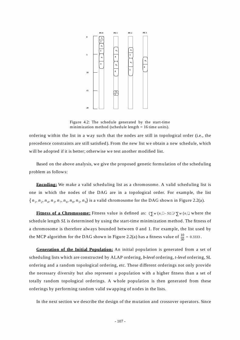
- 107 -

ordering within the list in a way such that the nodes are still in topological order (i.e., the

precedence constraints are still satisfied). From the new list we obtain a new schedule, which

will be adopted if it is better; otherwise we test another modified list.

Based on the above analysis, we give the proposed genetic formulation of the scheduling

problem as follows:

Encoding: We make a valid scheduling list as a chromosome. A valid scheduling list is

one in which the nodes of the DAG are in a topological order. For example, the list

is a valid chromosome for the DAG shown in Figure 2.2(a).

Fitness of a Chromosome: Fitness value is defined as: , where the

schedule length SL is determined by using the start-time minimization method. The fitness of

a chromosome is therefore always bounded between 0 and 1. For example, the list used by

the MCP algorithm for the DAG shown in Figure 2.2(a) has a fitness value of .

Generation of the Initial Population: An initial population is generated from a set of

scheduling lists which are constructed by ALAP ordering, b-level ordering, t-level ordering, SL

ordering and a random topological ordering, etc. These different orderings not only provide

the necessary diversity but also represent a population with a higher fitness than a set of

totally random topological orderings. A whole population is then generated from these

orderings by performing random valid swapping of nodes in the lists.

In the next section we describe the design of the mutation and crossover operators. Since

PE 0 PE 1 PE 2

n1

2

n2

3

n5

5

n91

n3

3n7

4

n4

4

0

5

10

15

20

n8

4

n6

4

Figure 4.2: The schedule generated by the start-timeminimization method (schedule length = 16 time units).

PE 3

n1 n2 n4 n3 n7 n6 n8 n5 n9, , , , , , , ,{ }

w ni( ) SL–∑( ) w ni( )∑⁄

1030------ 0.3333=

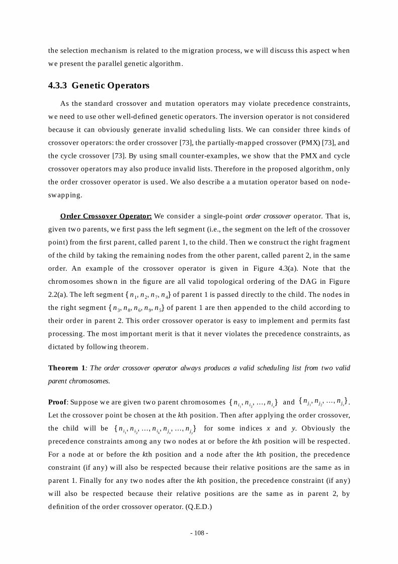
- 108 -

the selection mechanism is related to the migration process, we will discuss this aspect when

we present the parallel genetic algorithm.

4.3.3 Genetic Operators

As the standard crossover and mutation operators may violate precedence constraints,

we need to use other well-defined genetic operators. The inversion operator is not considered

because it can obviously generate invalid scheduling lists. We can consider three kinds of

crossover operators: the order crossover [73], the partially-mapped crossover (PMX) [73], and

the cycle crossover [73]. By using small counter-examples, we show that the PMX and cycle

crossover operators may also produce invalid lists. Therefore in the proposed algorithm, only

the order crossover operator is used. We also describe a a mutation operator based on node-

swapping.

Order Crossover Operator: We consider a single-point order crossover operator. That is,

given two parents, we first pass the left segment (i.e., the segment on the left of the crossover

point) from the first parent, called parent 1, to the child. Then we construct the right fragment

of the child by taking the remaining nodes from the other parent, called parent 2, in the same

order. An example of the crossover operator is given in Figure 4.3(a). Note that the

chromosomes shown in the figure are all valid topological ordering of the DAG in Figure

2.2(a). The left segment of parent 1 is passed directly to the child. The nodes in

the right segment of parent 1 are then appended to the child according to

their order in parent 2. This order crossover operator is easy to implement and permits fast

processing. The most important merit is that it never violates the precedence constraints, as

dictated by following theorem.

Theorem 1: The order crossover operator always produces a valid scheduling list from two valid

parent chromosomes.

Proof: Suppose we are given two parent chromosomes and .

Let the crossover point be chosen at the kth position. Then after applying the order crossover,

the child will be for some indices x and y. Obviously the

precedence constraints among any two nodes at or before the kth position will be respected.

For a node at or before the kth position and a node after the kth position, the precedence

constraint (if any) will also be respected because their relative positions are the same as in

parent 1. Finally for any two nodes after the kth position, the precedence constraint (if any)

will also be respected because their relative positions are the same as in parent 2, by

definition of the order crossover operator. (Q.E.D.)

n1 n2 n7 n4, , ,{ }

n3 n8 n6 n9 n5, , , ,{ }

ni1ni2

… niv, , ,{ } nj1

nj2… njv

, , ,{ }

ni1ni2

… niknjx

… njy, , , , , ,{ }

- 109 -

The order crossover operator as defined above has the potential to properly combine the

accurate task orderings of the two parent chromosomes so as to generate a scheduling list

which can lead to a shorter schedule. This is because the “good” portions of a parent

chromosome constitute a subsequence of the list, which is an optimal scheduling ordering of

the nodes in the subsequence. These good portions are essentially the building-blocks of an

optimal list, and an order crossover operation can potentially pass such building-blocks to an

n1 n2 n7 n4 n3 n8 n6 n9 n5, , , , , , , ,{ }

n1 n4 n2 n3 n7 n6 n8 n5 n9, , , , , , , ,{ }

parent 1

parent 2

crossover point

n1 n2 n7 n4 n3 n6 n8 n5 n9, , , , , , , ,{ }

(a) An example of the order crossover operator.

n1 n2 n4 n7 n3 n6 n8 n5 n9, , , , , , , ,{ } n1 n2 n7 n4 n3 n6 n8 n5 n9, , , , , , , ,{ }

Mutated(swapped

and )n4 n7

(d) An example of the mutation operator.

Figure 4.3: Examples of the (a) order crossover, (b) PMXcrossover, (c) cycle crossover, and (d) mutation operators.

n1 n2 n7 n4 n3 n8 n6 n9 n5, , , , , , , ,{ }

n1 n4 n2 n3 n7 n6 n8 n5 n9, , , , , , , ,{ }

parent 1

parent 2

crossover point

n1 n2 n3 n4 n7 n6 n8 n5 n9, , , , , , , ,{ }

(b) An example of the PMX crossover operator.

n1 n2 n7 n4 n3 n8 n6 n9 n5, , , , , , , ,{ }

n1 n4 n2 n3 n7 n6 n8 n5 n9, , , , , , , ,{ }

parent 1

parent 2

n1 n4 n2 n3 n7 n8 n6 n5 n9, , , , , , , ,{ }

(c) An example of the cycle crossover operator.

- 110 -

offspring chromosome from which a shorter schedule may be obtained.

PMX Crossover Operator: A single point partially-mapped crossover can be

implemented as follows. First a random crossover point is chosen. Then we consider the

segments following the crossover point in both parents as the partial mapping of the genes to

be exchanged in the first parent to generate the child. To do this, we first take corresponding

genes from the two right segments of both parents, and then locate both these genes in the

first parent and exchange them. Thus a gene in the right segment of the first parent and a

gene at the same position in the second parent will define which genes in the first parent have

to be swapped to generate the child. An example of the crossover operator is given in Figure

4.3(b). The pairs , , and are situated at the same locations in both

parents (note that the pairs and are implicitly handled also). Their

corresponding positions in parent 1 are swapped to generate the child. Then the remaining

nodes in parent 1 are copied to the child to finish the crossover. Unfortunately, unlike the

order crossover operator, PMX crossover may produce invalid scheduling lists. An example

of such scenario is shown in Figure 4.4. As can be seen, in the resulting chromosome, the

positions of and violate their precedence relationship. This is also true for and .

Cycle Crossover Operator: A single point cycle crossover operator can be implemented

n3 n7,( ) n8 n6,( ) n9 n5,( )

n6 n8,( ) n5 n9,( )

n2 n4 n3 n5

n1

n5n4

n3n2

(a)

n1 n2 n4 n3 n5, , , ,{ }

n1 n3 n2 n5 n4, , , ,{ }

crossover point

n1 n4 n2 n5 n3, , , ,{ }

(b)

n1 n2 n4 n3 n5, , , ,{ }

n1 n3 n5 n2 n4, , , ,{ }

n1 n3 n4 n2 n5, , , ,{ }

(c)

Figure 4.4: (a) A simple task graph; (b) An example of generating an invalidordering of the graph by using the PMX crossover operator; (c) An example ofgenerating an invalid ordering of the graph by using the cycle crossover operator.

- 111 -

as follows. We start at position 1 in parent 1 and copy the gene to location 1 of the child. Then

we examine the gene at position 1 in parent 2. This gene cannot be copied to the child since

the child’s corresponding position has been occupied. We then locate this gene from parent 1

and suppose it is found in position i. We copy this gene to position i of the child. Similarly the

gene at position i in parent 2 cannot be copied. We again locate this gene from parent 1 and

copy it to the child. This process is repeated until we encounter a gene in parent 2 which has

already been copied to the child from parent 1. This completes one cycle. Another cycle is

then initiated at the earliest position of the child that has not been occupied and the copying

is performed from parent 2 to the child. Thus, in alternate cycles, the child inherits genes from

both parents and the genes are copied at the same locations.

An example of the crossover operator is given in Figure 4.3(c). As can be seen in the

figure, is first copied to the child from parent 1. But the corresponding node in parent 2 is

also and, therefore, a cycle is completed. We start over again at position 2 of parent 2. We

first copy from parent 2 to the child. Then we find that the node in position 2 of parent 1 is

so that we copy from parent 2 to position 3 of the child. This time the corresponding

node is and so we copy from parent 2 to position 5 of the child. Since the node in

position 5 of parent 1 is , we copy from parent 2 to position 4 of the child. Now we

encounter in parent 1 which has already been copied from parent 2 to the child. Thus, the

second cycle is completed. The third cycle starts from parent 1 again and nodes and are

copied to the child at positions 6 and 7, respectively. The last cycle starts from parent 2 again

and nodes and are copied to the child at position 8 and 9, respectively. Unfortunately

the cycle crossover operator may also generate invalid scheduling lists. An example of such a

situation is shown in Figure 4.4. As can be seen, after the crossover, the positions of and

violate their precedence relationship.

Since both the PMX crossover operator and the cycle crossover operator do not guarantee

valid scheduling lists, they are not employed in the proposed algorithm.

Mutation Operator: A valid topological order can be transformed into another

topological order by swapping some nodes. For example, the scheduling list used by the

MCP algorithm— —can be transformed into an optimal list

by swapping and . Not every pair of nodes can be

swapped without violating the precedence constraints. Two nodes are interchangeable if they

are not lying on the same path in the DAG. Using a pre-processing depth-first traversal of the

DAG, we can check whether two randomly selected nodes are interchangeable in a constant

time during the search. If so, we swap them and check the new schedule length. Such

n1

n1

n4

n2 n2

n7 n7

n3 n3

n4

n8 n6

n5 n9

n2 n4

n1 n4 n2 n3 n7 n6 n8 n5 n9, , , , , , , ,{ }

n1 n2 n4 n3 n7 n6 n8 n5 n9, , , , , , , ,{ } n2 n4

- 112 -

swapping essentially defines a random search neighborhood. The size of the neighborhood is

since there are pairs of interchangeable nodes. We define the mutation

operator as a swap of two interchangeable nodes in a given chromosome. This operator

captures the major characteristic of mutation, which is to randomly perturb the chromosome

in such a way that a lost genetic feature can be recovered when the population is becoming

homogeneous. An example is given in Figure 4.3(d) where two interchangeable nodes and

are randomly chosen and their positions in the list are swapped.

Note that both the order crossover operator and the mutation operator take time to

compute.

4.3.4 Control Parameters

As Tanese [180], [181] has suggested, if the parallel processors executing a parallel genetic

algorithm use heterogeneous control parameters, the diversity of the global population can

be more effectively sustained. To implement this strategy, we use adaptive control

parameters as suggested by Srinivas et al. [175]. The adaptive crossover rate is defined as

follows:

where is the maximum fitness value in the local population, is the average fitness

value, is the fitness value of the fitter parent for the crossover, and is a positive real

constant less than 1.

The adaptive mutation rate is defined as follows:

where f is the fitness value of the chromosome to be mutated and is a positive real

constant less than 1.

Using the above adaptive crossover and mutation rate, the best chromosome is protected

from disruption by crossover and mutation. On the other hand, when the population tends to

become more homogeneous, both rates increase because will be about the same as .

Thus, under such a situation, chromosomes are more likely to be perturbed. This helps to

prevent the search from converging pre-maturely to a sub-optimal solution. Note that even

though the initial setting of the crossover rate and mutation rate is the same for all the

parallel processors, the adaptive strategy gradually leads to the desired heterogeneity of the

parameters among the processors.

O v2( ) O C2v( )

n4

n7

O v( )

µc

µc

kc fmax f′–( )fmax favg–( )------------------------------,=

fmax favg

f′ kc

µc

µm

km fmax f–( )fmax favg–( )-----------------------------= ,

km

favg fmax

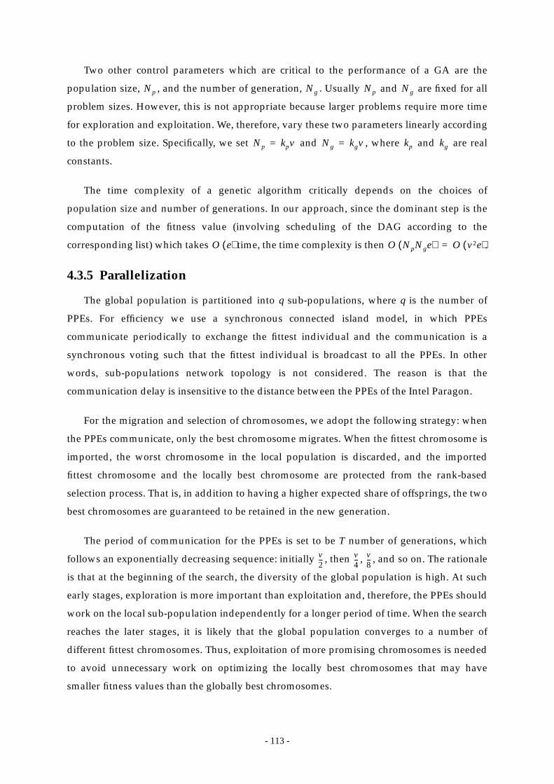
- 113 -

Two other control parameters which are critical to the performance of a GA are the

population size, , and the number of generation, . Usually and are fixed for all

problem sizes. However, this is not appropriate because larger problems require more time

for exploration and exploitation. We, therefore, vary these two parameters linearly according

to the problem size. Specifically, we set and , where and are real

constants.

The time complexity of a genetic algorithm critically depends on the choices of

population size and number of generations. In our approach, since the dominant step is the

computation of the fitness value (involving scheduling of the DAG according to the

corresponding list) which takes time, the time complexity is then .

4.3.5 Parallelization

The global population is partitioned into q sub-populations, where q is the number of

PPEs. For efficiency we use a synchronous connected island model, in which PPEs

communicate periodically to exchange the fittest individual and the communication is a

synchronous voting such that the fittest individual is broadcast to all the PPEs. In other

words, sub-populations network topology is not considered. The reason is that the

communication delay is insensitive to the distance between the PPEs of the Intel Paragon.

For the migration and selection of chromosomes, we adopt the following strategy: when

the PPEs communicate, only the best chromosome migrates. When the fittest chromosome is

imported, the worst chromosome in the local population is discarded, and the imported

fittest chromosome and the locally best chromosome are protected from the rank-based

selection process. That is, in addition to having a higher expected share of offsprings, the two

best chromosomes are guaranteed to be retained in the new generation.

The period of communication for the PPEs is set to be T number of generations, which

follows an exponentially decreasing sequence: initially , then , , and so on. The rationale

is that at the beginning of the search, the diversity of the global population is high. At such

early stages, exploration is more important than exploitation and, therefore, the PPEs should

work on the local sub-population independently for a longer period of time. When the search

reaches the later stages, it is likely that the global population converges to a number of

different fittest chromosomes. Thus, exploitation of more promising chromosomes is needed

to avoid unnecessary work on optimizing the locally best chromosomes that may have

smaller fitness values than the globally best chromosomes.

Np Ng Np Ng

Np kpv= Ng kgv= kp kg

O e( ) O NpNge( ) O v2e( )=

v2--- v

4--- v

8---

- 114 -

With the above design considerations, the Parallel Genetic Scheduling (PGS) algorithm is

outlined below.

Parallel Genetic Scheduling (PGS):(1) Generate a local population with size equal to by perturbing a pre-defined

topological ordering of the DAG (e.g., ALAP ordering, b-level ordering, etc.).(2) ;(3) repeat(4) ;(5) repeat(6) Using the current crossover and mutation rates, applied the operators to the

local population.(7) until ++T = ;(8) Accept the best chromosome from a remote PPE and discard the worst local

chromosome accordingly.(9) Explicitly protect the best local and remote chromosome and adapt new

crossover and mutation rates.(10)(11) until the total number of generations elapsed equal to ;


To examine the efficacy of the proposed PGS algorithm, we have implemented it on the

Intel Paragon using the C language and tested it with different suites of task graphs. In the

first two experiments, we aimed to investigate the absolute solution quality of the algorithm

by applying it to two different sets of random task graphs for which the optimal solutions are

known. These are the type-1 and type-2 random task graphs described in Section 3.5.4. Since

they have been used for testing the PFAST algorithm, the PGS algorithm is then indirectly

compared with the PFAST algorithm. Using random graphs with diverse parameters is

appropriate for testing the robustness of the PGS algorithm.

In the third experiment, we compared the PGS algorithm with other efficient techniques

using a suite of regularly structured synthetic task graphs. The suite is composed of graphs

representing the parallel Gaussian elimination algorithm [130], the parallel Laplace equation

solver [130], and the parallel LU-decomposition algorithm [130]. As all these algorithms

operate on matrices, the sizes of the task graphs vary with the matrix-sizes N in that

. We used matrix-sizes from 9 to 18 with an increment of 1.

We chose two extreme algorithms for comparison. The first is the DCP algorithm [114]

which has been compared to the best known six heuristic algorithms (DLS [172], MCP [189],

MD [189], ETF [93], DSC [193], and EZ [160]), and is known to be considerably better in terms

of performance but has a moderately higher complexity. The other is the DSC algorithm

Np q⁄

i 2=

T 0=

Ng i⁄

i i 2×=Ng

v O N2( )=

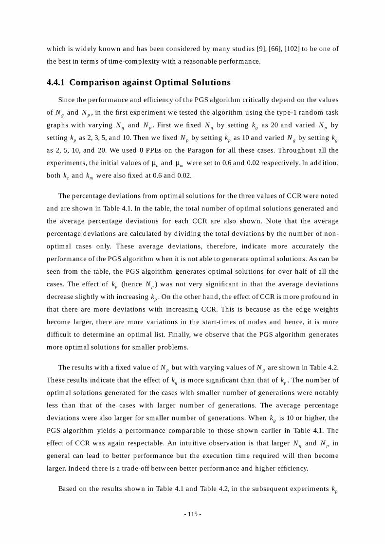
- 115 -

which is widely known and has been considered by many studies [9], [66], [102] to be one of

the best in terms of time-complexity with a reasonable performance.

4.4.1 Comparison against Optimal Solutions

Since the performance and efficiency of the PGS algorithm critically depend on the values

of and , in the first experiment we tested the algorithm using the type-1 random task

graphs with varying and . First we fixed by setting as 20 and varied by

setting as 2, 3, 5, and 10. Then we fixed by setting as 10 and varied by setting

as 2, 5, 10, and 20. We used 8 PPEs on the Paragon for all these cases. Throughout all the

experiments, the initial values of and were set to 0.6 and 0.02 respectively. In addition,

both and were also fixed at 0.6 and 0.02.

The percentage deviations from optimal solutions for the three values of CCR were noted

and are shown in Table 4.1. In the table, the total number of optimal solutions generated and

the average percentage deviations for each CCR are also shown. Note that the average

percentage deviations are calculated by dividing the total deviations by the number of non-

optimal cases only. These average deviations, therefore, indicate more accurately the

performance of the PGS algorithm when it is not able to generate optimal solutions. As can be

seen from the table, the PGS algorithm generates optimal solutions for over half of all the

cases. The effect of (hence ) was not very significant in that the average deviations

decrease slightly with increasing . On the other hand, the effect of CCR is more profound in

that there are more deviations with increasing CCR. This is because as the edge weights

become larger, there are more variations in the start-times of nodes and hence, it is more

difficult to determine an optimal list. Finally, we observe that the PGS algorithm generates

more optimal solutions for smaller problems.

The results with a fixed value of but with varying values of are shown in Table 4.2.

These results indicate that the effect of is more significant than that of . The number of

optimal solutions generated for the cases with smaller number of generations were notably

less than that of the cases with larger number of generations. The average percentage

deviations were also larger for smaller number of generations. When is 10 or higher, the

PGS algorithm yields a performance comparable to those shown earlier in Table 4.1. The

effect of CCR was again respectable. An intuitive observation is that larger and in

general can lead to better performance but the execution time required will then become

larger. Indeed there is a trade-off between better performance and higher efficiency.

Based on the results shown in Table 4.1 and Table 4.2, in the subsequent experiments

Ng Np

Ng Np Ng kg Np

kp Np kp Ng kg

µc µm

kc km

kp Np

kp

Np Ng

kg kp

kg

Ng Np

kp

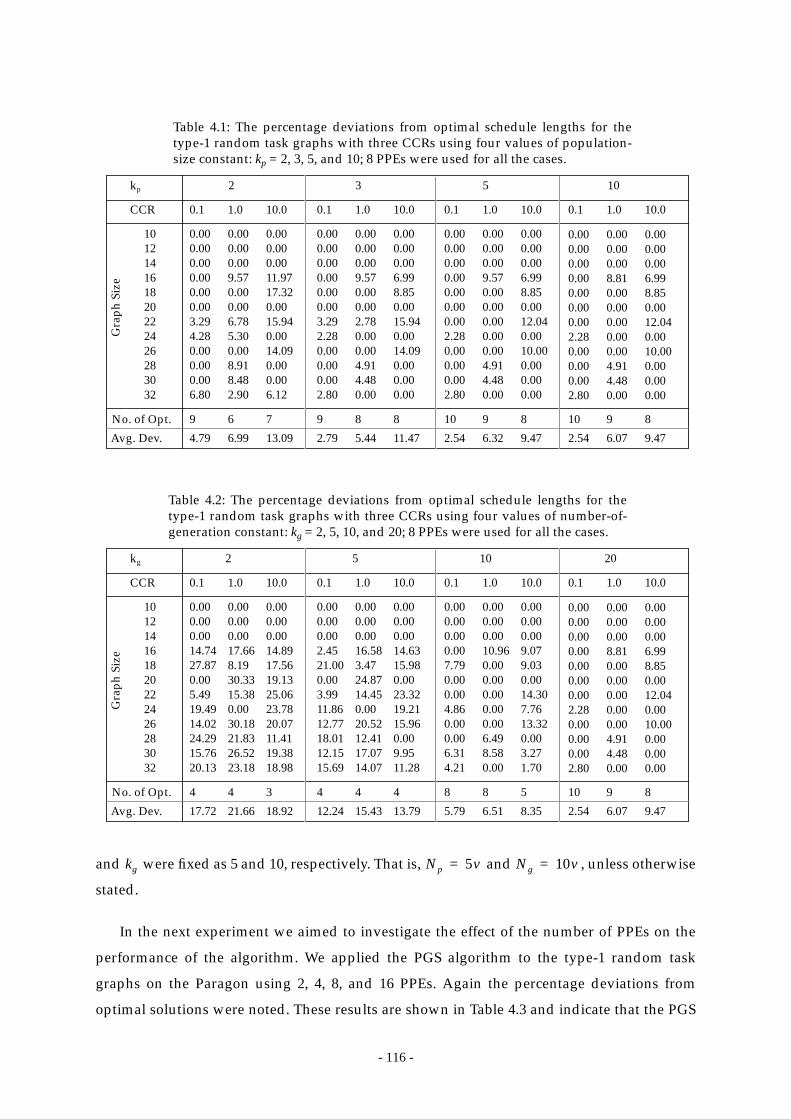
- 116 -

and were fixed as 5 and 10, respectively. That is, and , unless otherwise

stated.

In the next experiment we aimed to investigate the effect of the number of PPEs on the

performance of the algorithm. We applied the PGS algorithm to the type-1 random task

graphs on the Paragon using 2, 4, 8, and 16 PPEs. Again the percentage deviations from

optimal solutions were noted. These results are shown in Table 4.3 and indicate that the PGS

101214161820222426283032

0.00 0.00 0.000.00 0.00 0.000.00 0.00 0.000.00 9.57 11.970.00 0.00 17.320.00 0.00 0.003.29 6.78 15.944.28 5.30 0.000.00 0.00 14.090.00 8.91 0.000.00 8.48 0.006.80 2.90 6.12

0.00 0.00 0.000.00 0.00 0.000.00 0.00 0.000.00 9.57 6.990.00 0.00 8.850.00 0.00 0.003.29 2.78 15.942.28 0.00 0.000.00 0.00 14.090.00 4.91 0.000.00 4.48 0.002.80 0.00 0.00

0.00 0.00 0.000.00 0.00 0.000.00 0.00 0.000.00 9.57 6.990.00 0.00 8.850.00 0.00 0.000.00 0.00 12.042.28 0.00 0.000.00 0.00 10.000.00 4.91 0.000.00 4.48 0.002.80 0.00 0.00

0.00 0.00 0.000.00 0.00 0.000.00 0.00 0.000.00 8.81 6.990.00 0.00 8.850.00 0.00 0.000.00 0.00 12.042.28 0.00 0.000.00 0.00 10.000.00 4.91 0.000.00 4.48 0.002.80 0.00 0.00

Gra

ph S

ize

0.1 1.0 10.0

2

0.1 1.0 10.0

3

0.1 1.0 10.0

5

0.1 1.0 10.0

10

No. of Opt. 9 6 7 9 8 8 10 9 8 10 9 8

Avg. Dev. 4.79 6.99 13.09 2.79 5.44 11.47 2.54 6.32 9.47 2.54 6.07 9.47

Table 4.1: The percentage deviations from optimal schedule lengths for thetype-1 random task graphs with three CCRs using four values of population-size constant: kp = 2, 3, 5, and 10; 8 PPEs were used for all the cases.

kp

CCR

101214161820222426283032

0.00 0.00 0.000.00 0.00 0.000.00 0.00 0.0014.74 17.66 14.8927.87 8.19 17.560.00 30.33 19.135.49 15.38 25.0619.49 0.00 23.7814.02 30.18 20.0724.29 21.83 11.4115.76 26.52 19.3820.13 23.18 18.98

0.00 0.00 0.000.00 0.00 0.000.00 0.00 0.002.45 16.58 14.6321.00 3.47 15.980.00 24.87 0.003.99 14.45 23.3211.86 0.00 19.2112.77 20.52 15.9618.01 12.41 0.0012.15 17.07 9.9515.69 14.07 11.28

0.00 0.00 0.000.00 0.00 0.000.00 0.00 0.000.00 10.96 9.077.79 0.00 9.030.00 0.00 0.000.00 0.00 14.304.86 0.00 7.760.00 0.00 13.320.00 6.49 0.006.31 8.58 3.274.21 0.00 1.70

0.00 0.00 0.000.00 0.00 0.000.00 0.00 0.000.00 8.81 6.990.00 0.00 8.850.00 0.00 0.000.00 0.00 12.042.28 0.00 0.000.00 0.00 10.000.00 4.91 0.000.00 4.48 0.002.80 0.00 0.00

Gra

ph S

ize

0.1 1.0 10.0

2

0.1 1.0 10.0

5

0.1 1.0 10.0

10

0.1 1.0 10.0

20

No. of Opt. 4 4 3 4 4 4 8 8 5 10 9 8

Avg. Dev. 17.72 21.66 18.92 12.24 15.43 13.79 5.79 6.51 8.35 2.54 6.07 9.47

Table 4.2: The percentage deviations from optimal schedule lengths for thetype-1 random task graphs with three CCRs using four values of number-of-generation constant: kg = 2, 5, 10, and 20; 8 PPEs were used for all the cases.

kg

CCR

kg Np 5v= Ng 10v=

- 117 -

algorithm yields a similar performance for 2, 4, and 8 PPEs. When 16 PPEs were used, the

performance degraded by a slightly larger margin. One explanation for this phenomenon is

that using more PPEs implies a smaller local population size, which in turn leads to smaller

diversity of the local population. Premature convergence is then more likely to result. The

effect of CCR is again quite considerable in that the average deviations increase with

increasing CCRs.

To examine the effectiveness of parallelization, we observed the execution times of the

PGS algorithm using different number of PPEs. As a reference, we also ran the PGS algorithm

using 1 PPE on the Paragon. The average execution times and speedups are shown in Figure

4.5. These averages were computed across the three values of CCR. As can be seen from the

speedup plot, the PGS algorithm exhibits a slightly less than linear speedup because the

migration of best chromosomes contributed considerable communication overhead.

From the above results we find that the number of generations used critically affects the

performance of the PGS algorithm. In view of this, we ran the algorithm with larger number

of generations to see how far it could approach optimal. We used 8 PPEs on the Paragon and

left the other parameters the same. The results of which are shown in Figure 4.6. Note that the

results for the smaller number of generations shown earlier in Table 4.2 are also included. We

notice that when the number of generations is increased to , the PGS algorithm is almost

optimal.

101214161820222426283032

Gra

ph S

ize

No. of Opt.

Avg. Dev.

Table 4.3: Results of the PGS algorithm compared against optimalsolutions (percentage deviations) for the type-1 random task graphswith three CCRs using 2, 4, 8, and 16 PPEs on the Intel Paragon.

CCR

No. of PPEs

0.00 0.00 0.00 7.960.00 0.00 0.00 5.050.00 0.00 0.00 9.287.59 6.71 6.17 16.287.98 7.23 7.23 7.720.00 0.00 0.00 0.2613.02 12.09 11.99 24.406.16 5.35 5.21 12.0210.23 10.19 9.65 32.500.00 0.00 0.00 10.292.30 2.25 2.09 2.331.20 1.05 1.03 1.98

2 4 8 16

10.0

5 5 5 0

6.93 6.41 6.20 10.84

0.00 0.00 0.00 3.140.00 0.00 0.00 16.350.00 0.00 0.00 5.419.23 8.05 7.87 17.780.00 0.00 0.00 5.230.00 0.00 0.00 10.960.00 0.00 0.00 17.980.00 0.00 0.00 10.270.00 0.00 0.00 9.416.07 5.24 5.12 10.416.32 5.26 4.88 11.010.00 0.00 0.00 13.16

2 4 8 16

1.0

9 9 9 0

7.21 6.18 5.96 10.93

0.00 0.00 0.00 0.000.00 0.00 0.00 2.320.00 0.00 0.00 0.000.86 0.62 0.60 0.676.15 5.18 5.01 5.990.00 0.00 0.00 5.300.00 0.00 0.00 4.574.01 3.31 2.89 5.086.57 5.30 5.04 14.584.66 3.20 3.11 7.164.27 2.59 2.16 4.533.34 2.31 2.11 3.30

2 4 8 16

0.1

5 5 5 2

4.27 3.22 2.99 5.35

40v

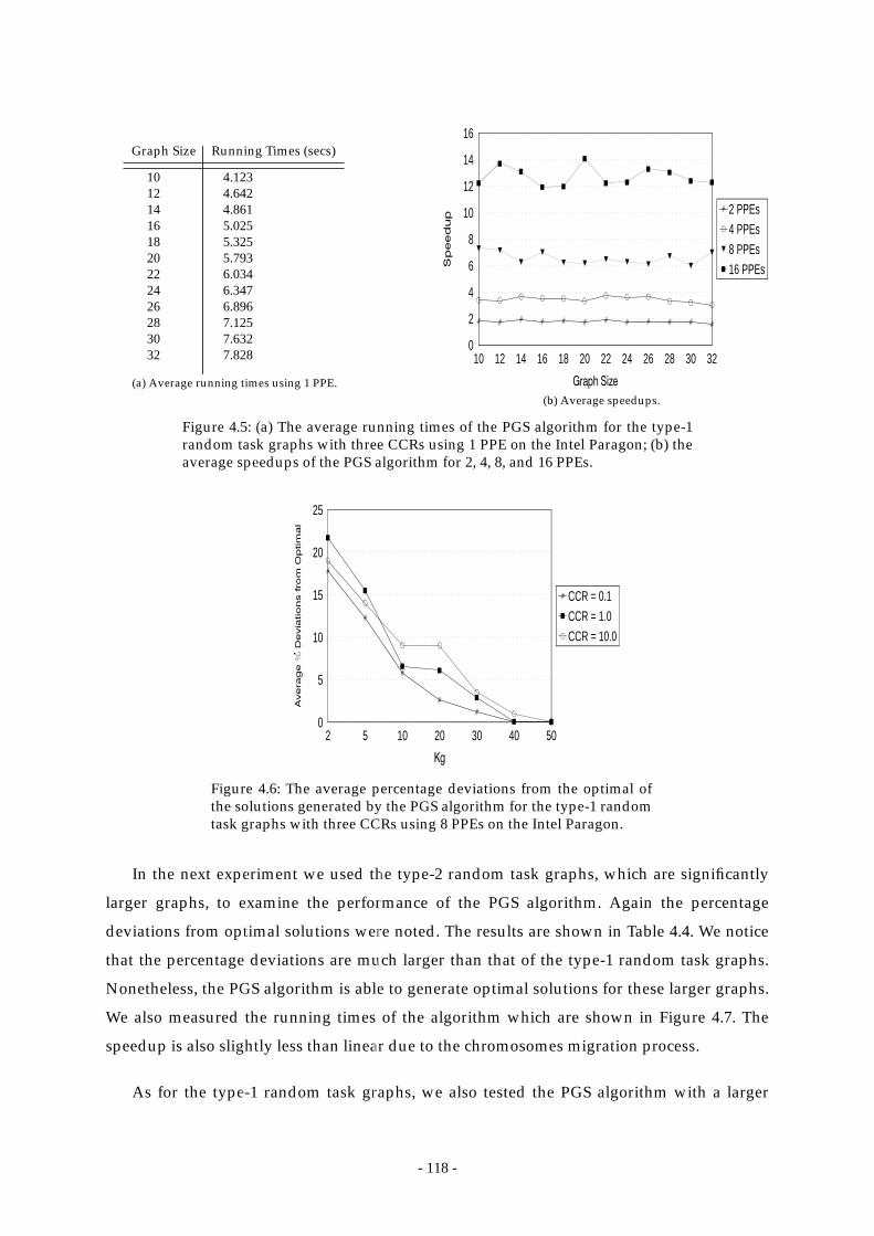
- 118 -

In the next experiment we used the type-2 random task graphs, which are significantly

larger graphs, to examine the performance of the PGS algorithm. Again the percentage

deviations from optimal solutions were noted. The results are shown in Table 4.4. We notice

that the percentage deviations are much larger than that of the type-1 random task graphs.

Nonetheless, the PGS algorithm is able to generate optimal solutions for these larger graphs.

We also measured the running times of the algorithm which are shown in Figure 4.7. The

speedup is also slightly less than linear due to the chromosomes migration process.

As for the type-1 random task graphs, we also tested the PGS algorithm with a larger

10 12 14 16 18 20 22 24 26 28 30 320

2

4

6

8

10

12

14

16



Figure 4.5: (a) The average running times of the PGS algorithm for the type-1random task graphs with three CCRs using 1 PPE on the Intel Paragon; (b) theaverage speedups of the PGS algorithm for 2, 4, 8, and 16 PPEs.


101214161820222426283032

Graph Size

4.1234.6424.8615.0255.3255.7936.0346.3476.8967.1257.6327.828


2 5 10 20 30 40 500

5

10

15

20

25

CCR = 0.1CCR = 1.0CCR = 10.0

Figure 4.6: The average percentage deviations from the optimal ofthe solutions generated by the PGS algorithm for the type-1 randomtask graphs with three CCRs using 8 PPEs on the Intel Paragon.

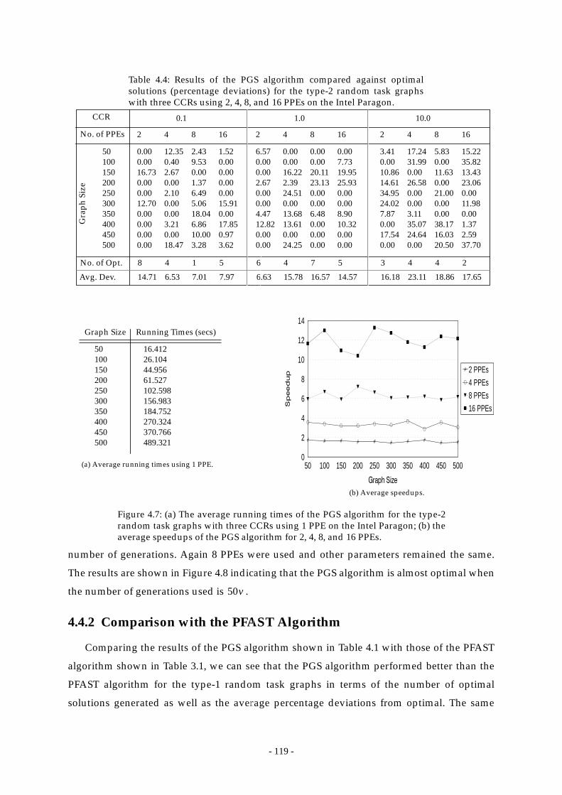
- 119 -

number of generations. Again 8 PPEs were used and other parameters remained the same.

The results are shown in Figure 4.8 indicating that the PGS algorithm is almost optimal when

the number of generations used is .

4.4.2 Comparison with the PFAST Algorithm

Comparing the results of the PGS algorithm shown in Table 4.1 with those of the PFAST

algorithm shown in Table 3.1, we can see that the PGS algorithm performed better than the

PFAST algorithm for the type-1 random task graphs in terms of the number of optimal

solutions generated as well as the average percentage deviations from optimal. The same

50100150200250300350400450500

Gra

ph S

ize

No. of Opt.

Avg. Dev.

Table 4.4: Results of the PGS algorithm compared against optimalsolutions (percentage deviations) for the type-2 random task graphswith three CCRs using 2, 4, 8, and 16 PPEs on the Intel Paragon.

CCR

No. of PPEs

3.41 17.24 5.83 15.220.00 31.99 0.00 35.8210.86 0.00 11.63 13.4314.61 26.58 0.00 23.0634.95 0.00 21.00 0.0024.02 0.00 0.00 11.987.87 3.11 0.00 0.000.00 35.07 38.17 1.3717.54 24.64 16.03 2.590.00 0.00 20.50 37.70

2 4 8 16

10.0

3 4 4 2

16.18 23.11 18.86 17.65

6.57 0.00 0.00 0.000.00 0.00 0.00 7.730.00 16.22 20.11 19.952.67 2.39 23.13 25.930.00 24.51 0.00 0.000.00 0.00 0.00 0.004.47 13.68 6.48 8.9012.82 13.61 0.00 10.320.00 0.00 0.00 0.000.00 24.25 0.00 0.00

2 4 8 16

1.0

6 4 7 5

6.63 15.78 16.57 14.57

0.00 12.35 2.43 1.520.00 0.40 9.53 0.0016.73 2.67 0.00 0.000.00 0.00 1.37 0.000.00 2.10 6.49 0.0012.70 0.00 5.06 15.910.00 0.00 18.04 0.000.00 3.21 6.86 17.850.00 0.00 10.00 0.970.00 18.47 3.28 3.62

2 4 8 16

0.1

8 4 1 5

14.71 6.53 7.01 7.97

50 100 150 200 250 300 350 400 450 5000

2

4

6

8

10

12

14



Figure 4.7: (a) The average running times of the PGS algorithm for the type-2random task graphs with three CCRs using 1 PPE on the Intel Paragon; (b) theaverage speedups of the PGS algorithm for 2, 4, 8, and 16 PPEs.


50100150200250300350400450500

Graph Size

16.41226.10444.95661.527102.598156.983184.752270.324370.766489.321


50v

- 120 -

observation can be made for the type-2 random task graphs when the results shown in Table

4.2 are compared with that shown in Table 3.2. However, these findings have to be

complemented by the results of the algorithm running times. Indeed, when we compare the

running times of both algorithms which are shown in Figure 4.5 and Figure 3.8 for type-1

random task graphs, and Figure 4.7 and Figure 3.9 for type-2 random task graphs, it is

obvious that the PFAST algorithm is much faster than the PGS algorithm in that the former

used two orders of magnitude less time to generate solutions than did the latter. Thus, while

the PGS algorithm has a higher capability to generate optimal solutions, the PFAST algorithm

has a higher efficiency. Which one of the two is more suitable depends on the particular

scheduling objectives in terms of running time allowed and quality of solution expected.

4.4.3 Results on Regular Graphs

In the last experiment we aimed to compare the performance of the PGS algorithm with

the DSC [193] and DCP algorithms. We used three sets of regular task graphs representing

three parallel numerical algorithms: Gaussian elimination, LU-decomposition, and Laplace

equation solver. The size of these graphs vary with the input matrix sizes for these numerical

algorithms. We used 10 graphs for each CCR with matrix sizes varying from 9 to 18. The sizes

of the 10 graphs then varied roughly from 30 to 300. It should be noted that these graphs are

sparse graphs compared with the random graphs used in the previous experiments.

As optimal solutions for these regular graphs are not available, we computed the ratios of

the schedule lengths generated by the PGS algorithm to that of the DSC and DCP algorithm

using 2, 4, 8, and 16 PPEs on the Paragon. The results of comparing the PGS algorithm with

2 5 10 20 30 40 500

10

20

30

40

50

CCR = 0.1CCR = 1.0CCR = 10.0

Figure 4.8: The average percentage deviations from the optimal ofthe solutions generated by the PGS algorithm for the type-2 randomtask graphs with three CCRs using 8 PPEs on the Intel Paragon.

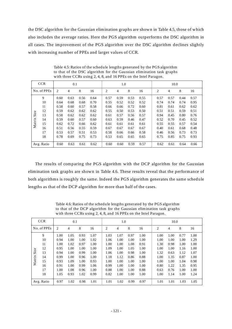
- 121 -

the DSC algorithm for the Gaussian elimination graphs are shown in Table 4.5, those of which

also includes the average ratios. Here the PGS algorithm outperforms the DSC algorithm in

all cases. The improvement of the PGS algorithm over the DSC algorithm declines slightly

with increasing number of PPEs and larger values of CCR.

The results of comparing the PGS algorithm with the DCP algorithm for the Gaussian

elimination task graphs are shown in Table 4.6. These results reveal that the performance of

both algorithms is roughly the same. Indeed the PGS algorithm generates the same schedule

lengths as that of the DCP algorithm for more than half of the cases.

9101112131415161718

Mat

rix

Size

Avg. Ratio

Table 4.5: Ratios of the schedule lengths generated by the PGS algorithmto that of the DSC algorithm for the Gaussian elimination task graphswith three CCRs using 2, 4, 8, and 16 PPEs on the Intel Paragon.

CCR

No. of PPEs

0.57 0.57 0.44 0.570.74 0.74 0.74 0.950.81 0.61 0.62 0.620.51 0.51 0.59 0.510.94 0.45 0.80 0.760.52 0.70 0.45 0.520.55 0.55 0.57 0.540.40 0.61 0.68 0.480.46 0.56 0.73 0.730.75 0.85 0.75 0.93

2 4 8 16

10.0

0.62 0.61 0.64 0.66

0.57 0.59 0.53 0.550.55 0.52 0.52 0.520.66 0.66 0.72 0.600.55 0.50 0.53 0.500.61 0.57 0.56 0.570.63 0.59 0.46 0.470.61 0.61 0.61 0.610.67 0.67 0.67 0.670.58 0.66 0.66 0.580.53 0.65 0.65 0.65

2 4 8 16

1.0

0.60 0.60 0.59 0.57

0.60 0.63 0.56 0.640.64 0.68 0.68 0.700.58 0.60 0.57 0.580.59 0.62 0.62 0.620.58 0.62 0.62 0.620.59 0.60 0.57 0.600.62 0.72 0.66 0.620.51 0.56 0.55 0.590.53 0.57 0.51 0.530.78 0.69 0.75 0.73

2 4 8 16

0.1

0.60 0.63 0.61 0.62

9101112131415161718

Mat

rix

Size

Avg. Ratio

Table 4.6: Ratios of the schedule lengths generated by the PGS algorithmto that of the DCP algorithm for the Gaussian elimination task graphswith three CCRs using 2, 4, 8, and 16 PPEs on the Intel Paragon.

CCR

No. of PPEs

1.00 1.00 0.77 1.001.00 1.00 1.00 1.291.30 0.98 1.00 1.001.00 1.00 1.16 1.001.32 0.63 1.12 1.071.00 1.35 0.87 1.001.00 1.00 1.04 0.980.80 1.22 1.35 0.950.63 0.76 1.00 1.001.00 1.14 1.00 1.24

2 4 8 16

10.0

1.01 1.01 1.03 1.05

1.03 1.07 0.97 1.001.06 1.00 1.00 1.001.00 1.00 1.08 0.911.09 1.00 1.05 1.001.06 1.00 0.98 1.001.18 1.12 0.86 0.881.00 1.00 1.00 1.000.99 1.00 1.00 1.000.88 1.00 1.00 0.880.82 1.00 1.00 1.00

2 4 8 16

1.0

1.01 1.02 0.99 0.97

1.00 1.05 0.93 1.070.94 1.00 1.00 1.021.00 1.02 0.97 1.000.95 1.00 1.00 1.000.94 1.00 0.99 1.000.99 1.00 0.96 1.000.93 1.09 1.00 0.930.91 1.00 0.99 1.061.00 1.08 0.96 1.001.05 0.93 1.02 0.99

2 4 8 16

0.1

0.97 1.02 0.98 1.01

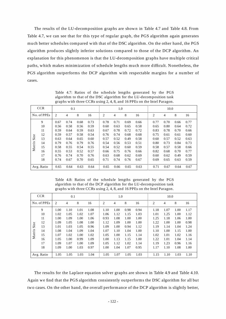
- 122 -

The results of the LU-decomposition graphs are shown in Table 4.7 and Table 4.8. From

Table 4.7, we can see that for this type of regular graph, the PGS algorithm again generates

much better schedules compared with that of the DSC algorithm. On the other hand, the PGS

algorithm produces slightly inferior solutions compared to those of the DCP algorithm. An

explanation for this phenomenon is that the LU-decomposition graphs have multiple critical

paths, which makes minimization of schedule lengths much more difficult. Nonetheless, the

PGS algorithm outperforms the DCP algorithm with respectable margins for a number of

cases.

The results for the Laplace equation solver graphs are shown in Table 4.9 and Table 4.10.

Again we find that the PGS algorithm consistently outperforms the DSC algorithm for all but

two cases. On the other hand, the overall performance of the DCP algorithm is slightly better,

9101112131415161718

Mat

rix

Size

Avg. Ratio

Table 4.7: Ratios of the schedule lengths generated by the PGSalgorithm to that of the DSC algorithm for the LU-decomposition taskgraphs with three CCRs using 2, 4, 8, and 16 PPEs on the Intel Paragon.

CCR

No. of PPEs

0.77 0.70 0.66 0.770.65 0.80 0.64 0.720.83 0.78 0.70 0.660.75 0.61 0.61 0.600.60 0.57 0.52 0.630.80 0.73 0.84 0.730.58 0.57 0.58 0.660.82 0.68 0.70 0.770.60 0.62 0.49 0.590.69 0.65 0.63 0.59

2 4 8 16

10.0

0.71 0.67 0.64 0.67

0.78 0.71 0.69 0.660.60 0.63 0.65 0.580.67 0.78 0.72 0.720.76 0.74 0.68 0.680.57 0.52 0.49 0.580.54 0.56 0.53 0.510.54 0.52 0.60 0.590.66 0.75 0.76 0.660.63 0.68 0.62 0.690.71 0.74 0.76 0.67

2 4 8 16

1.0

0.65 0.66 0.65 0.63

0.67 0.74 0.68 0.730.56 0.58 0.56 0.590.59 0.64 0.59 0.630.59 0.57 0.58 0.540.63 0.64 0.65 0.600.79 0.76 0.79 0.760.58 0.55 0.54 0.550.55 0.53 0.52 0.570.76 0.74 0.70 0.760.74 0.67 0.70 0.65

2 4 8 16

0.1

0.65 0.64 0.63 0.64

9101112131415161718

Mat

rix

Size

Avg. Ratio

Table 4.8: Ratios of the schedule lengths generated by the PGSalgorithm to that of the DCP algorithm for the LU-decomposition taskgraphs with three CCRs using 2, 4, 8, and 16 PPEs on the Intel Paragon.

CCR

No. of PPEs

1.18 1.07 1.00 1.171.01 1.25 1.00 1.121.25 1.18 1.06 1.001.22 1.00 1.00 0.981.19 1.14 1.04 1.241.10 1.00 1.15 1.001.02 1.01 1.02 1.161.22 1.01 1.04 1.141.19 1.23 0.96 1.161.17 1.10 1.08 1.00

2 4 8 16

10.0

1.15 1.10 1.03 1.10

1.10 1.00 0.98 0.941.06 1.12 1.15 1.030.93 1.08 1.00 1.001.12 1.09 1.00 1.001.09 1.00 0.94 1.121.07 1.10 1.04 1.001.05 1.00 1.15 1.141.00 1.13 1.15 1.001.05 1.12 1.02 1.141.00 1.04 1.07 0.95

2 4 8 16

1.0

1.05 1.07 1.05 1.03

1.00 1.10 1.01 1.081.02 1.05 1.02 1.071.00 1.09 1.00 1.061.09 1.05 1.08 1.001.01 1.03 1.05 0.961.08 1.04 1.09 1.041.07 1.02 1.00 1.021.05 1.00 0.99 1.091.09 1.07 1.00 1.091.09 1.00 1.03 0.97

2 4 8 16

0.1

1.05 1.05 1.03 1.04

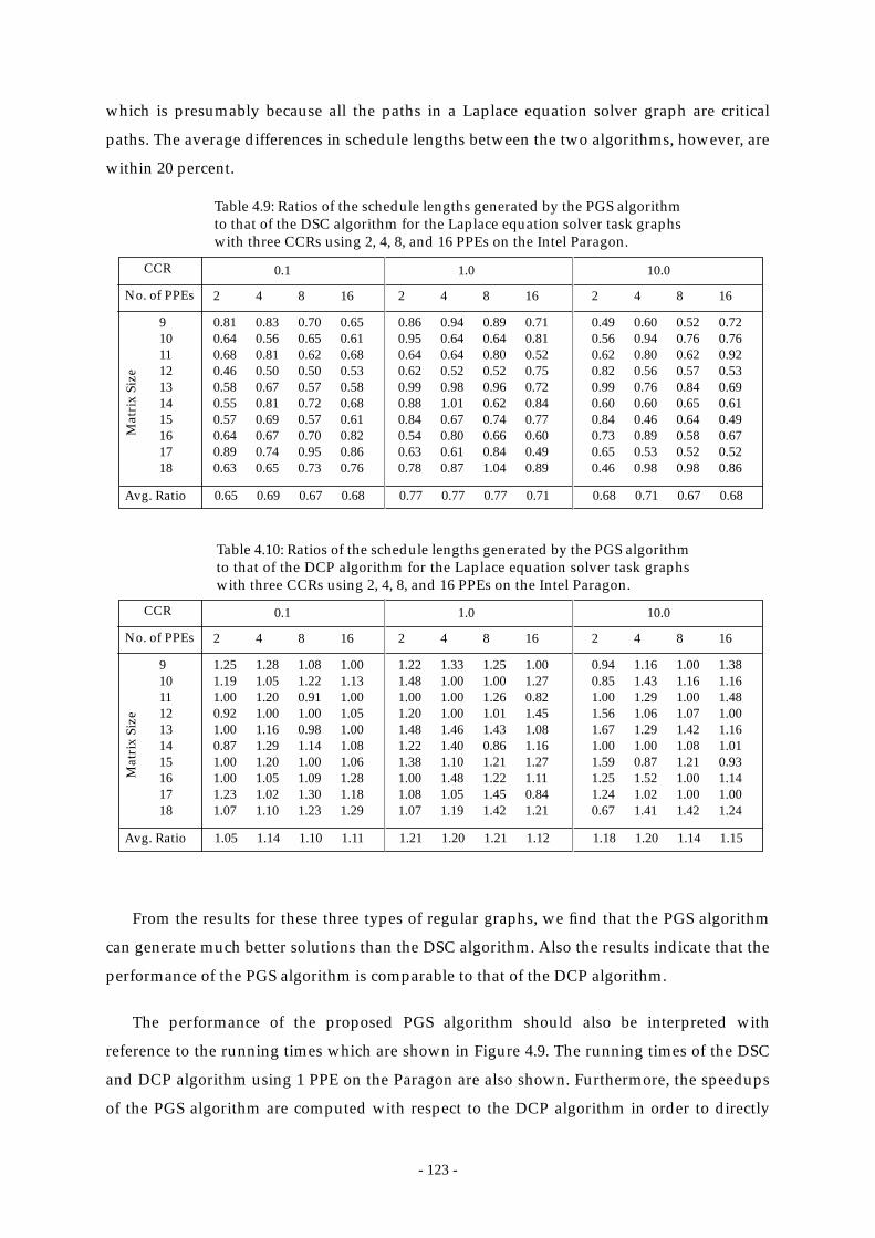
- 123 -

which is presumably because all the paths in a Laplace equation solver graph are critical

paths. The average differences in schedule lengths between the two algorithms, however, are

within 20 percent.

From the results for these three types of regular graphs, we find that the PGS algorithm

can generate much better solutions than the DSC algorithm. Also the results indicate that the

performance of the PGS algorithm is comparable to that of the DCP algorithm.

The performance of the proposed PGS algorithm should also be interpreted with

reference to the running times which are shown in Figure 4.9. The running times of the DSC

and DCP algorithm using 1 PPE on the Paragon are also shown. Furthermore, the speedups

of the PGS algorithm are computed with respect to the DCP algorithm in order to directly

9101112131415161718

Mat

rix

Size

Avg. Ratio

Table 4.9: Ratios of the schedule lengths generated by the PGS algorithmto that of the DSC algorithm for the Laplace equation solver task graphswith three CCRs using 2, 4, 8, and 16 PPEs on the Intel Paragon.

CCR

No. of PPEs

0.49 0.60 0.52 0.720.56 0.94 0.76 0.760.62 0.80 0.62 0.920.82 0.56 0.57 0.530.99 0.76 0.84 0.690.60 0.60 0.65 0.610.84 0.46 0.64 0.490.73 0.89 0.58 0.670.65 0.53 0.52 0.520.46 0.98 0.98 0.86

2 4 8 16

10.0

0.68 0.71 0.67 0.68

0.86 0.94 0.89 0.710.95 0.64 0.64 0.810.64 0.64 0.80 0.520.62 0.52 0.52 0.750.99 0.98 0.96 0.720.88 1.01 0.62 0.840.84 0.67 0.74 0.770.54 0.80 0.66 0.600.63 0.61 0.84 0.490.78 0.87 1.04 0.89

2 4 8 16

1.0

0.77 0.77 0.77 0.71

0.81 0.83 0.70 0.650.64 0.56 0.65 0.610.68 0.81 0.62 0.680.46 0.50 0.50 0.530.58 0.67 0.57 0.580.55 0.81 0.72 0.680.57 0.69 0.57 0.610.64 0.67 0.70 0.820.89 0.74 0.95 0.860.63 0.65 0.73 0.76

2 4 8 16

0.1

0.65 0.69 0.67 0.68

9101112131415161718

Mat

rix

Size

Avg. Ratio

Table 4.10: Ratios of the schedule lengths generated by the PGS algorithmto that of the DCP algorithm for the Laplace equation solver task graphswith three CCRs using 2, 4, 8, and 16 PPEs on the Intel Paragon.

CCR

No. of PPEs

0.94 1.16 1.00 1.380.85 1.43 1.16 1.161.00 1.29 1.00 1.481.56 1.06 1.07 1.001.67 1.29 1.42 1.161.00 1.00 1.08 1.011.59 0.87 1.21 0.931.25 1.52 1.00 1.141.24 1.02 1.00 1.000.67 1.41 1.42 1.24

2 4 8 16

10.0

1.18 1.20 1.14 1.15

1.22 1.33 1.25 1.001.48 1.00 1.00 1.271.00 1.00 1.26 0.821.20 1.00 1.01 1.451.48 1.46 1.43 1.081.22 1.40 0.86 1.161.38 1.10 1.21 1.271.00 1.48 1.22 1.111.08 1.05 1.45 0.841.07 1.19 1.42 1.21

2 4 8 16

1.0

1.21 1.20 1.21 1.12

1.25 1.28 1.08 1.001.19 1.05 1.22 1.131.00 1.20 0.91 1.000.92 1.00 1.00 1.051.00 1.16 0.98 1.000.87 1.29 1.14 1.081.00 1.20 1.00 1.061.00 1.05 1.09 1.281.23 1.02 1.30 1.181.07 1.10 1.23 1.29

2 4 8 16

0.1

1.05 1.14 1.10 1.11

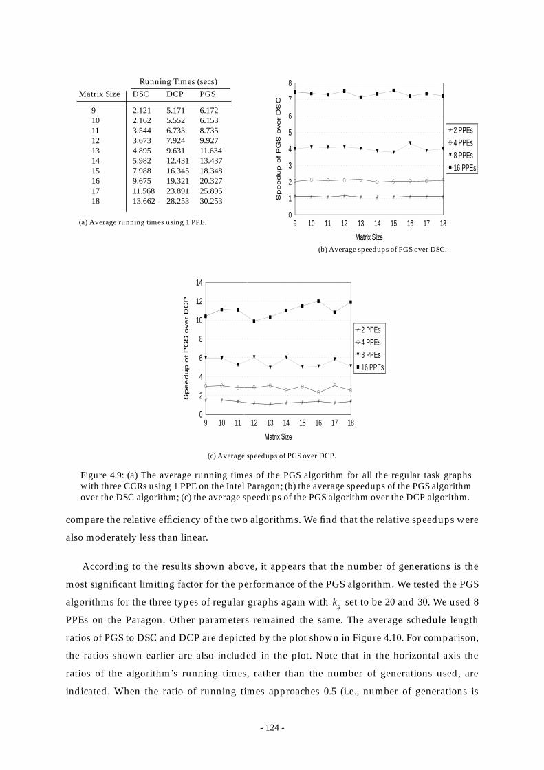
- 124 -

compare the relative efficiency of the two algorithms. We find that the relative speedups were

also moderately less than linear.

According to the results shown above, it appears that the number of generations is the

most significant limiting factor for the performance of the PGS algorithm. We tested the PGS

algorithms for the three types of regular graphs again with set to be 20 and 30. We used 8

PPEs on the Paragon. Other parameters remained the same. The average schedule length

ratios of PGS to DSC and DCP are depicted by the plot shown in Figure 4.10. For comparison,

the ratios shown earlier are also included in the plot. Note that in the horizontal axis the

ratios of the algorithm’s running times, rather than the number of generations used, are

indicated. When the ratio of running times approaches 0.5 (i.e., number of generations is

9 10 11 12 13 14 15 16 17 180

2

4

6

8

10

12

14


9 10 11 12 13 14 15 16 17 180

1

2

3

4

5

6

7

8



Figure 4.9: (a) The average running times of the PGS algorithm for all the regular task graphswith three CCRs using 1 PPE on the Intel Paragon; (b) the average speedups of the PGS algorithmover the DSC algorithm; (c) the average speedups of the PGS algorithm over the DCP algorithm.

(b) Average speedups of PGS over DSC.

9101112131415161718

Matrix Size

5.1715.5526.7337.9249.63112.43116.34519.32123.89128.253


6.1726.1538.7359.92711.63413.43718.34820.32725.89530.253

DCP PGS

(c) Average speedups of PGS over DCP.

2.1212.1623.5443.6734.8955.9827.9889.67511.56813.662

DSC

kg

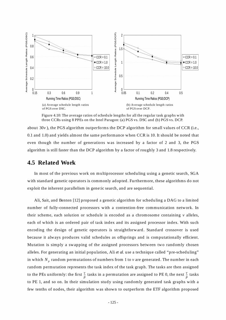
- 125 -

about ), the PGS algorithm outperforms the DCP algorithm for small values of CCR (i.e.,

0.1 and 1.0) and yields almost the same performance when CCR is 10. It should be noted that

even though the number of generations was increased by a factor of 2 and 3, the PGS

algorithm is still faster than the DCP algorithm by a factor of roughly 3 and 1.8 respectively.

4.5 Related Work

In most of the previous work on multiprocessor scheduling using a genetic search, SGA

with standard genetic operators is commonly adopted. Furthermore, these algorithms do not

exploit the inherent parallelism in genetic search, and are sequential.

Ali, Sait, and Benten [12] proposed a genetic algorithm for scheduling a DAG to a limited

number of fully-connected processors with a contention-free communication network. In

their scheme, each solution or schedule is encoded as a chromosome containing v alleles,

each of which is an ordered pair of task index and its assigned processor index. With such

encoding the design of genetic operators is straightforward. Standard crossover is used

because it always produces valid schedules as offsprings and is computationally efficient.

Mutation is simply a swapping of the assigned processors between two randomly chosen

alleles. For generating an initial population, Ali et al. use a technique called “pre-scheduling”

in which random permutations of numbers from 1 to v are generated. The number in each

random permutation represents the task index of the task graph. The tasks are then assigned

to the PEs uniformly: the first tasks in a permutation are assigned to PE 0, the next tasks

to PE 1, and so on. In their simulation study using randomly generated task graphs with a

few tenths of nodes, their algorithm was shown to outperform the ETF algorithm proposed

0.15 0.3 0.6 0.9 10

0.2

0.4

0.6

0.8

1

CCR = 0.1CCR = 1.0CCR = 10.0

0.05 0.1 0.2 0.4 0.50

0.5

1

1.5

2

CCR = 0.1CCR = 1.0CCR = 10.0

Figure 4.10: The average ratios of schedule lengths for all the regular task graphs withthree CCRs using 8 PPEs on the Intel Paragon: (a) PGS vs. DSC and (b) PGS vs. DCP.

(b) Average schedule length ratiosof PGS over DCP.

(a) Average schedule length ratiosof PGS over DSC.

30v

Np

vp--- v

p---

- 126 -

by Hwang et al. [93].

Hou, Ansari, and Ren [89] also proposed a scheduling algorithm using genetic search in

which each chromosome is a collection of lists, and each list represents the schedule on a

distinct processor. Thus, each chromosome is not a linear structure but a two-dimensional

structure instead. One dimension is a particular processor index and the other is the ordering

of tasks scheduled on the processor. Using such an encoding scheme poses a restriction on

the schedules being represented: the list of tasks within each processor in a schedule is

ordered in ascending order of their topological height, which is defined as the largest number

of edges from an entry node to the node itself. This restriction also facilitates the design of the

crossover operator. In a crossover, two processors are selected from each of two

chromosomes. The list of tasks on each processor is cut into two parts and then the two

chromosomes exchange the two lower parts of their task lists correspondingly. It is shown

that this crossover mechanism always produces valid offsprings. However, the height

restriction in the encoding may cause the search to be incapable of obtaining the optimal

solution because the optimal solution may not obey the height ordering restriction at all.

Hou et al. incorporated a heuristic technique to lower the likelihood of such pathological

situation. Mutation is simpler in design. In a mutation, two randomly chosen tasks with the

same height are swapped in the schedule. As to the generation of the initial population,

randomly permuted schedules obeying the height ordering restriction are generated. In their

simulation study using randomly generated task graphs with a few tenths of nodes, their

algorithm was shown to produce schedules within 20 percent from optimal solutions.

Ahmad and Dhodhi [2] proposed a scheduling algorithm using a variant of genetic

algorithm called simulated evolution. They employ a problem-space neighborhood

formulation in that a chromosome represents a list of task priorities. Since task priorities are

dependent on the input DAG, different set of task priorities represent different problem

instances. First, a list of priorities is obtained from the input DAG. Then the initial population

of chromosomes are generated by randomly perturbing this original list. Standard genetic

operators are applied to these chromosomes to determine the fittest chromosome which is the

one giving the shortest schedule length for the original problem. The genetic search, therefore,

operates on the problem-space instead of the solution-space as is commonly done. The

rationale of this approach is that good solutions of the problem instances in the problem-

space neighborhood are expected to be good solutions for the original problem as well [179].

Np

- 127 -


We have presented a parallel genetic algorithm, called the PGS algorithm, for

multiprocessor DAG scheduling. The major motivation of using a genetic search approach is

that the recombinative nature of a genetic algorithm can potentially determine an optimal

scheduling list leading to an optimal schedule. Using well-defined crossover and mutation

operators, the PGS algorithm judiciously combines good building-blocks of scheduling lists

to construct better lists. Parallelization of the algorithm is based on a novel approach in that

the parallel processors communicate to exchange the best chromosomes with exponentially

decreasing periods. As such, the parallel processors perform exploration of the solution-space

at the early stages and exploitation at the later stages.

In our experimental studies, we have found that the PGS algorithm generates optimal

solutions for more than half of all the cases in which random task graphs were used. In

addition, the PGS algorithm demonstrates an almost linear speedup and is therefore scalable.

We have also compared the PGS algorithm with the PFAST algorithm presented in Chapter 3.

We find that while the PGS algorithm has a higher capability in generating optimal solutions,

the PFAST algorithm has a higher efficiency. Which one of the two is more suitable depends

on the particular scheduling environments in terms of running time allowed and quality of

solution expected.

While the DCP algorithm has already been shown to outperform many of the leading

algorithms, the PGS algorithm is even better since it generates solutions with comparable

quality while using significantly less time due to its effective parallelization. The PGS

algorithm outperforms the DSC algorithm in terms of both the solution quality and running

time. An extra advantage of the PGS algorithm is its scalability, and with the use of more

parallel processors, the algorithm can be used for scheduling large task graphs.

Although the PGS algorithm has shown encouraging performance, further improvements

may be possible if we can determine an optimal set of control parameters, including

crossover rate, mutation rate, population size, number of generations, and number of parallel

processors used. However, finding an optimal parameters set for a particular genetic

algorithm is hitherto an open research problem.

- 128 -

Chapter 5

A Parallel Algorithm for APN Scheduling

5.1 Introduction

In this chapter, we propose a parallel algorithm for scheduling under the most

unrestricted environment: the algorithm is applicable given arbitrary computation and

communication costs, arbitrary network topology, link contention and underlying message-

routing strategy. As such the proposed algorithm belongs to the APN scheduling algorithms

class (a detailed taxonomy is provided in Chapter 2). Furthermore, the algorithm also

considers heterogeneity of target processors. The algorithm, called the Parallel Bubble

Scheduling and Allocation (PBSA) algorithm, is implemented on the Intel Paragon.

The proposed PBSA algorithm gives high quality solutions without requiring any of the

preceding simplifying assumptions. Specifically, the algorithm can handle regular or

irregular graph structures with arbitrary communication and computation costs, and works

for arbitrarily connected networks of processors. It also schedules messages on the network

by taking into account link contention. The message scheduling mechanism can be adapted

to any specific routing strategy. Moreover, it is designed to handle processors with identical

or different speeds, and therefore is applicable to distributed systems as well.

The organization of this chapter is as follows. In Section 5.2, we first introduce the

sequential version of the PBSA algorithm and discuss its design principles. We then describe

the parallelization method and present the PBSA algorithm. In Section 5.3, an example is

used to illustrate the algorithms. In Section 5.4, we present the results of our experimental

studies and compare it with three other APN algorithms. We summarize the chapter in the

last section.

5.2 The Proposed Algorithm

In this section, we describe the proposed parallel algorithm for APN scheduling. The

algorithm, called the Parallel Bubble Scheduling and Allocation (PBSA) algorithm, incrementally

- 129 -

optimizes the scheduling of tasks and messages to a network of processors with an arbitrary

connection topology. In the following, we first explicate the process of incremental node

migrations. The graph partitioning and parallelization issues are discussed afterwards.

5.2.1 Scheduling Serially

To explain the node migration process, we consider the special case that only a single

processing element is used to execute the PBSA algorithm. We refer to the serialized

algorithm simply as the BSA algorithm.

In the scheduling of a task graph for an arbitrary network of processors, scheduling of

communication messages must be carefully handled lest the schedule length increases.

However, in previous approaches the message scheduling issue has not been tackled

satisfactorily. Usually the message scheduling scheme has to be supplied as a routing table

for the scheduler. The routing table is used when a processor is being considered for

accommodating a node. From the routing table, the possible routes reaching this processor

from the node’s parents have to be examined. The scheduling algorithm has to know whether

each and every link in a route has been occupied during the period of communication.

Checking such routing information for every candidate processors inevitably results in high

time-complexity. Moreover, the routing information is either statically hard-wired in the

routing table (as in the BU algorithm [135]) or dynamically updated (as in the MH algorithm

[50]). In the static approach, the routing information is inflexible and may not be appropriate

so that some messages may be competing for some links while other links are idle. In the

dynamic approach, to maintain accurate routing information, the routing table needs to be

frequently updated, thus, the scheduling algorithm may have high time-complexity.

Furthermore, in either approach, the routing information is usually maintained for only a few

common network topologies which may not be useful for an arbitrary network.

To cope with the message routing and scheduling problem, we employ an incremental

adaptive approach. The task graph is first serialized through the CPN-Dominant sequence

(refer to Section 2.6.5.6 for a detailed discussion) which is then injected into a single

processor, called the pivot processor, which is the one with the largest number of links. This

process is called serial injection. The CPN-Dominant sequence is used because it can capture

the relative importance of nodes for scheduling. The nodes are then incrementally “bubbled-

up” by migration to the adjacent processors in a breadth-first order. In the course of node

migration, messages are also incrementally routed and scheduled to the most suitable time

slots on an optimized route. This is because a node will not migrate if its start-time cannot be

- 130 -

reduced by the migration or the destination processor for migration is not a valid choice as

specified by the underlying routing scheme.

A candidate node for migration is a node that has its data arrival time (DAT)—defined as

the time at which the last message from its parent nodes finishes delivery—earlier than its

current start-time on the pivot processor. The goal of the migration is to schedule the node to

an earlier time slot on one of the adjacent processors that allows the largest reduction of the

start-time of the node. To determine the largest start-time reduction, we need to compute the

DAT and the start-time of the node on each adjacent processor. Simply put, a node can be

scheduled to a processor if the processor has an idle time slot that is later than the node’s

DAT and is large enough to accommodate the node. The following rule formalizes the

computation of the start-time of a node on a processor.

Rule I: A node can be scheduled to a processor P in which m nodes have

been scheduled if there exists some k such that

where , , and . The start-time of on

processor P is given by with l being the smallest k satisfying

the above inequality.

Rule I states that to determine the start-time of a node on a processor, we have to examine

the first idle time slot, if any, before the first node on that processor. We check whether the

overlapping portion, if any, of the idle time slot and the time period in which the node can

start execution, is large enough to accommodate the node. If there is such an idle time slot,

the start-time for the node is the earliest one; if not, we proceed to try the next idle time slot.

The DAT of a node on a processor is constrained by the finish-times of the parent nodes

and the message arrival times. If the node under consideration and its parent node are

scheduled to the same processor, the message arrival time of this parent node is simply its

finish-time on the processor (intra-processor communication time is ignored). On the other

hand, if the parent node is scheduled to another processor, the message arrival time depends

on how the message is routed and scheduled on the links. To schedule a message on a link,

we can view the link as a resource similar to a processor and search for a suitable idle time

slot on the link to accommodate the message. Simply put, a message can be scheduled to a

link if the link has an idle time slot that is later than the source node’s finish-time and is large

enough to accommodate the message. Rule II, which is similar to Rule I, formalizes the

scheduling of a message to a link.

ni nP1nP2

… nPm, , ,{ }

ST nPk 1+P,( ) max FT nPk

P,( ) DAT ni P,( ),{ }– w ni( )≥

k 0 … m, ,= ST nPm 1+P,( ) ∞= FT nP0

P,( ) 0= ni

max FT nPlP,( ) DAT ni P,( ),{ }

- 131 -

Rule II: A message can be scheduled to a link L on which m messages

have been scheduled if there exists some k such that

where and , . The start-time of on L,

denoted by , is given by with r being the

smallest k satisfying the above inequality.

Rule II states that to determine the start-time of a message on a link, we have to examine

the first idle time slot, if any, before the first message on that link. We check whether the

overlapping portion, if any, of the idle time slot and the time period in which the message can

start transmission, is large enough to accommodate the message. If not, we proceed to try the

next idle time slot. If there is indeed one such idle time slot, the start-time for the message is

the earliest one.

The DAT of the node on the processor is then simply the largest value of the message

arrival times. The parent node that corresponds to this largest value of the message arrival

time is called the Very Important Parent (VIP).

It should be noted that in Rule II we do not explicitly model the underlying message

switching technique of the target processor network. Thus, we can insert an appropriate

method for modeling whether the messages are wormhole routed or circuit-switched. In a

wormhole-routed network, messages are broken up into fixed-size portions called flits. Thus,

a message normally does not occupy the whole route simultaneously in the course of

communication. By contrast, in a circuit-switched network, a message occupies all the links

involved in its route for the whole time period of communication.

In our approach, messages are automatically routed in the migration process of nodes

from the pivot processors to other processors. A node will only migrate from a processor to

its neighbor in each step, but multi-hop messages are routed incrementally after successive

iterations of node migrations. Thus, in our approach, there is no need to use a routing table.

The sequential BSA algorithm [111], [113] is outlined below. The procedure

Build_processor_list() constructs a list of processors in a breadth-first order from the first pivot

processor. The procedure Serial_injection() constructs the CPN-Dominant sequence of the nodes

and injects all the nodes to the first pivot processor.

ex ni nj,( )=

e1 … em, ,{ }MST ek 1+ L,( ) max MFT ek L,( ) FT ni Proc ni( ),( ),{ } cij≥–

k 0 … m, ,= MST em 1+ L,( ) ∞= MFT eo L,( ) 0= ex

MST ex L,( ) max MFT er 1+ L,( ) FT ni Proc ni( ),( ),{ }

- 132 -

The Bubble Scheduling and Allocation Algorithm:(1) Load processor topology and input task graph(2) Pivot_TPE ← the processor with the highest degree(3) Build_processor_list(Pivot_TPE)(4) Serial_injection(Pivot_TPE)(5) while Processor_list_not_empty do(6) Pivot_TPE ← first processor of Processor_list(7) for each ni on Pivot_TPE do(8) if ST(ni, Pivot_TPE) > DAT(ni, Pivot_TPE) or Proc(VIP(ni)) ≠ Pivot_TPE then(9) Determine DAT and ST of ni on each adjacent processor PE’(10) if there exists a PE’ s.t. ST(ni, PE’) < ST(ni, Pivot_TPE) then(11) Make ni to migrate from Pivot_TPE to PE’(12) Update start-times of nodes and messages(13) else if ST(ni,PE’) = ST(ni,Pivot_TPE) and Proc(VIP(ni)) = PE’ then(14) Make ni to migrate from Pivot_TPE to PE’(15) Update start-times of nodes and messages(16) end if(17) end if(18) end for(19) end while

If the target processors are heterogeneous, the decision as to whether a migration should

be taken is determined by the finish-times of the nodes rather than the start-times. This is

because for heterogeneous processors, the execution time of a task varies for different

processors; hence, even if a task can start at the same time for two distinct processors, its

finish-times can be different. Moreover, the first pivot processor will be the one on which the

CP length is the shortest in order to further minimize the finish-times of the CPNs by

exploiting the heterogeneity of the processors.

The procedure Build_processor_list() takes time because it involves a breadth-first

traversal of the processor graph. The procedure Serial_injection() takes time because

the CPN-Dominant sequence can be constructed in time. Thus, the dominant step is

the while-loop from step (5) to step (19). In this loop, it takes O(e) time to compute the ST and

DAT values of the node on each adjacent processor. If migration is done, it also takes O(e)

time. Since there are O(v) nodes on the Pivot_TPE and O(p) adjacent processors, each iteration

of the while loop takes O(pev) time. Thus, the BSA algorithm takes time. Notice that

this time-complexity is comparable to those of other APN algorithms surveyed in Chapter 2.

The above incremental scheduling method can also be extended to heterogeneous

processors in the following manner: the decision as to whether a migration should be taken is

determined by the finish-times of the nodes rather than the start-times. Moreover, the first

pivot processor will be the one for which the CP length is the shortest so as to further

O p2( )

O e v+( )

O e v+( )

O p2ev( )

- 133 -

minimize the finish-times of the CPNs by exploiting the heterogeneity of the processors.

5.2.2 Scheduling in Parallel

Having expounded the node migration process with reference to the serialized algorithm,

we now explicate the parallelization aspects of the PBSA algorithm.

In the following, again we call the processors which execute the PBSA algorithm the

physical processing elements (PPEs) in order to distinguish them from the target processing

elements (TPEs) to which the task graph is to be scheduled.

Parallelization is based on partitioning of the DAG. In simpler terms, a DAG can be

partitioned horizontally or vertically. Partitioning of the DAG horizontally means dividing it

into layers of nodes such that the paths in the DAG are sectioned by the layers. In contrast,

partitioning of the DAG vertically means dividing it along the paths. The partitioned pieces

can then be scheduled independently and their resultant schedules can be concatenated.

However, a naive horizontal or vertical partitioning is inappropriate because it can be

sensitive to the graph structure. In the PBSA algorithm, we partition the CPN-Dominant

sequence (which is neither vertical nor horizontal but is a combination of the two). The

number of partitions is equal to the number of PPEs available. Each PPE independently

schedules the nodes in its own partition by using a sequential BSA algorithm. After the sub-

schedules for all the partitions are generated, they are concatenated to form the final

complete schedule.

Due to the dependencies between the nodes of two adjacent partitions, global

information sharing between PPEs is required in the scheduling process. When a PPE

attempts to schedule a node in its partition, it has to know the finish-time of a parent node in

another partition, called the remote parent node (RPN), so that it can determine the earliest

start-time. A straightforward approach is to let the PPEs communicate and exchange

information about the start-times in the scheduling process. This approach, however, is not

efficient because revisions of local schedules in the PPEs are needed and communication can

be an excessive overhead which limits the speedup. In our approach, estimated information

is used in each PPE so that inter-PPE communication is minimized. These estimates are given

in the following definitions.

Definition 5.1: The earliest possible start-time (EPST) of a node is the largest sum of

computation costs from an entry node to the node but not including the node itself.

Definition 5.2: The latest possible start-time (LPST) of a node is the sum of computation costs

- 134 -

from the first node in the serial injection ordering to the node but not including the node

itself.

On the one hand, the start-time of a node is bounded below by its EPST due to the

precedence constraints. On the other hand, the start-time is also bounded from above by the

node’s LPST because LPST is the start-time of the node when the DAG is serialized by the

serial injection process. The EPST and LPST are, therefore, respectively the most optimistic

estimate and the most pessimistic estimate for the start-time of any RPN.

An RPN can legitimately be scheduled to start at any time between these two extremes.

The problem is to pick an accurate estimate for a RPN’s start-time from all values between

the two extremes. In our approach, if the RPN is a CPN, we take an optimistic estimate for its

start-time; otherwise, we take a conservative estimate. Specifically, the estimated start-time of

a RPN is taken to be its EPST if it is a CPN; otherwise, it is taken to be

where the importance factor is a positive real number less than 1.

In addition to the estimated start-time of an RPN, we need to know to which TPE the

RPN is scheduled. This is essential in determining the DAT of a node to be scheduled and, in

turn, in choosing the most suitable TPE for the node. We estimate this in the following

manner: if the RPN is a CPN, then we assume that it will be scheduled to the same TPE as the

highest level CPN in the local partition; otherwise, we just randomly pick one TPE to be the

one to which the RPN is scheduled. We call this TPE of an RPN the estimated TPE (ETPE).

In the PBSA algorithm, a PPE is designated as the master and the other PPEs slaves. The

master PPE is responsible for all pre-scheduling and post-scheduling work. This includes the

serial injection process, the task graph partitioning process, the concatenation of sub-

schedules, and resolving any conflicts in sub-schedules. It should be noted that both EST and

ETPE of any RPN can be statically determined by the master program after the graph

partitioning process. The slave procedure of PBSA is outlined below.

Procedure PBSA_Slave():(1) Receive the target processor network from PBSA_Master().(2) Receive graph partition together with the RPN’s information (i.e., estimated start-

times and TPEs) from PBSA_Master().(3) Apply the serial BSA algorithm to the graph partition. For every RPN, its EST and

ETPE are used for determining the DAT of a node to be scheduled in the localpartition.

(4) Send the resulting sub-schedule to PBSA_Master().

To derive the time-complexity, suppose there are nodes in the local partition of

αEPST 1 α–( ) LPST+

α

m

- 135 -

PBSA_Slave(). As step (3) in PBSA_Slave() is the dominant step, the complexity of

PBSA_Slave() is , where is the number of edges in the local partition.

In the master procedure, the sub-schedules are to be concatenated. The concatenation

process involves a matching of TPEs between adjacent sub-schedules. Obviously an

exhaustive matching is not feasible so in order to reduce the time-complexity of sub-

schedules concatenation process, we employ a two-phase method. The objective of the first

phase is to minimize the start-time of the most important node in every sub-schedule. Such a

node is likely to be a CPN. The second phase is for rearranging the exit nodes (i.e., the nodes

without any successor in the same partition) of a sub-schedule so that they can start earlier.

This rearrangement can potentially make the most important node of the next sub-schedule

start earlier.

In the first phase, for every sub-schedule, the earliest node among all TPEs is determined.

Call this node the leader node and the TPE to which the leader node is scheduled the leader

TPE. The leader node, together with all its succeeding nodes on the leader TPE, are

concatenated to a TPE of its preceding sub-schedule such that the start-time of the leader

node is scheduled as early as possible. Such a TPE is called the image of the leader TPE. Then,

the neighboring TPEs of the leader TPE are concatenated to the corresponding neighboring

TPEs of the leader TPE’s image. This is done to all TPEs in a breadth-first manner. In the

concatenation process, nodes may need to be pushed down because of the scheduling of the

inter-partition communication messages. In addition, the communication messages in a sub-

schedule may need to use more communication links in the concatenated schedule because

two neighboring TPEs in the sub-schedule may not be mapped to two neighboring TPEs in

the concatenated schedule.

In the second phase, after a sub-schedule is concatenated with its preceding sub-

schedule, all exit nodes in the sub-schedule are examined for re-scheduling. Specifically, each

exit node is re-scheduled to the TPE which allows the minimum start-time.

The procedure for performing this two-phase concatenation process, called

Concat_Schedules(), is outlined below.

O p2e′m( ) e′

- 136 -

Procedure Concat_Schedules():(1) for every pair of adjacent sub-schedules, do(2) Determine the earliest node in the latter sub-schedule. Call this the leader node.

Call its TPE the leader TPE.(3) Concatenate all nodes, which are scheduled on the same TPE as the leader node,

to a TPE in the former sub-schedule so that the leader node can start as early aspossible.

(4) Concatenate the nodes on all other TPEs to the TPEs of the former sub-schedulein a breadth-first order beginning from the neighbors of the leader TPE.

(5) Re-schedule the exit nodes in the latter sub-schedule so that they can start asearly as possible.

(6) Walk through the whole concatenated schedule to resolve any conflict betweenthe actual start-times and the estimated start-times.

(7) end for

To derive the time-complexity, suppose that there are at most nodes in every sub-

schedule. Since step (2) and step (5) take time; while steps (3), (4), and (6) take

time, the time-complexity of Concat_Schedules() is then , where is the number of

PPEs (i.e., the number of sub-schedules).

With the procedure Concat_Schedules(), the master procedure of the PBSA algorithm can

be outlined below.

Procedure PBSA_Master():(1) Load processor network topology and input task graph.(2) Serial_injection()(3) Partition the task graph into equal sized sets according to the number of node PPEs

available. Determine the ESTs and ETPEs for every RPNs in all partitions.(4) Broadcast the processor network topology to all PBSA_Slave().(5) Send the particular graph partition together with the corresponding ESTs and ETPEs

to each PBSA_Slave().(6) Wait until all PBSA_Slave() finish.(7) Concat_Schedules()

As mentioned earlier, if the target processors are heterogeneous, the slave procedure, as

in the sequential BSA algorithm, can decide on whether to perform a migration based on the

finish-times rather than the start-times. In addition, it is the finish-times that are estimated in

order to determine the data arrival times. Furthermore, the processor on which the CP length

is the shortest will be taken as the first pivot processor.

If there are PPEs, the maximum size of each partition will then be . Thedominant steps in PBSA_Master() are steps (6) and (7). As described above, step (6) takes

and step (7) takes . The time-complexity of PBSA_Master() is then. Taking to be , the time-complexity is .

m

O m( ) O m2( )

O qm2( ) q

q m v q⁄

O p2e′m( ) O qm2( )O p2e′ v

P--- P v

P---

2+

e′ eP--- O p2 e

P--- v

P--- P v

P---

2+

- 137 -

It is interesting to analyze the theoretical speedup of the PBSA algorithm with respect to

the serial BSA algorithm. Let us denote the speedup by . We then have:

Dropping the ceiling operators, we have:

Since the second term in the denominator is much smaller than the first term, we ignore it

and get the following approximate theoretical speedup of PBSA over serial BSA:

That is, the speedup grows as the square of the number of PPEs used, which is superlinear.

This superlinear speedup is mainly due to the fact that the PBSA algorithm estimates start-

times of RPNs, thereby spending less time in scheduling inter-partition edges.

5.3 An Example

In this section, we present an example to demonstrate the operation of the BSA and PBSA

algorithms using a task graph shown in Figure 5.1(a). We examine the schedules generated

by the BSA algorithm for homogeneous and heterogeneous processors, and then the schedule

generated by the PBSA algorithm.

First, consider the schedule for a homogeneous target system consisting of a ring of 4 PEs.

The CPN-Dominant sequence is constructed as follows. The critical path of the task graph is

. Since is the entry CPN, it is placed in the first position in the CPN-Dominant

sequence. The second node is because it is another unexamined parent node of the next

CPN . After is appended to the CPN-Dominant sequence, all parent nodes of have

therefore been considered and so is also added to the sequence. The last CPN, cannot be

appended to the sequence because some of its parent nodes (i.e., the IBNs) have not been

examined yet. Since both and have the same value of b-level and has a smaller t-

level, is considered first. However, both parent nodes of have not been examined. Thus,

its two parent nodes, and are appended to the CPN-Dominant sequence first. Next,

is appended followed by . The only OBN, , is the last node in the CPN-Dominant

sequence. The final CPN-Dominant sequence is as follows: (see

Figure 5.1(b); the CPNs are marked by an asterisk).

SBSAPBSA

SBSAPBSA O p2ev

p2 eP--- v

P--- P v

P---

2+

-------------------------------------------------

.=

SBSAPBSA O p2ev

p2evP2

----------- v2

P-----+

-----------------------

O 11P2----- v

p2eP-----------+

------------------------

.= =

SBSAPBSA O P2( ) .=

n1 n7 n9, ,{ } n1

n2

n7 n2 n7

n9

n6 n8 n8

n8 n8

n3 n4 n8

n6 n5

n1 n2 n7 n4 n3 n8 n6 n, 9 n5, , , , , , ,

- 138 -

The BSA algorithm injects the CPN-Dominant sequence to the first pivot processor PE 0

(Figure 5.2(a)). In the first phase, n1, n2, and n7 do not migrate because they are already

scheduled to finish at the earliest possible times. But n4 migrates to PE 1 because its finish-

time improves. Also, n3 migrates to a neighboring processor PE 3. Similarly, n8 also migrated

to PE 1 to further reduce its finish-time. The intermediate schedule after these migrations is

shown in Figure 5.2(b). Next n6 migrates to PE 3 (Figure 5.2(c)). The last CPN, n9, migrates to

PE 1 to which its VIP n8 is scheduled. Such migration allows the only OBN n5 to move up.

The resulting schedule is shown in Figure 5.2(d), which is the final schedule as no more nodes

can improve the finish-time by migration. The final schedule length is 160. For this example,

we also ran the MH, DLS, and BU algorithm. The schedule length produced by both the MH

and DLS algorithms was 200. The BU algorithm yielded a schedule length of 270.

Now consider the scheduling for heterogeneous processors. We model heterogeneity by

making each task able to have different execution times on different processors. The task

execution times on each processor, randomly generated from a uniform distribution with

means being the execution times on homogeneous processors, are shown in Figure 5.3(a).

Given this table, the CPs on PE 0, PE 1, PE 2, and PE 3 are , ,

, and , respectively. The CP lengths are 240, 226, 235, and 260,

respectively. Thus, the first pivot processor is PE 1 as the CP length is the shortest on this

processor. The CPN-Dominant sequence is (which is different

from that for homogeneous processors). After serial injection, the intermediate schedule is

n1

20

n2

30

n5

50

n9

n3

30

n7

40

n4

40

n8

40

n6

40

10

60

100

10

1010

10

40

10

10

5050

(a)

(b)

node t-level b-level CPN-Dominant order

*n1 0 230 1n2 60 150 2n3 30 140 5n4 30 150 4n5 30 50 9n6 100 100 7*n7 120 110 3n8 80 100 6*n9 220 10 8

10

Figure 5.1: (a) A task graph; (b) The static levels(SLs) and the CPN-Dominant sequence of the nodes.

n1 n7 n9, ,{ } n1 n2 n6 n9, , ,{ }

n1 n2 n7 n9, , ,{ } n1 n2 n6 n9, , ,{ }

n1 n2 n6 n7 n, 3 n4 n8 n9 n5, , , , , , ,{ }

- 139 -

shown in Figure 5.3(b). In the first phase, n1, being the entry CPN, does not migrate because

its migration increases the data arrival times to its successors. Also, n2 and n6 do not migrate

because their finish-times cannot be improved by migration. However, n3 and n4 migrate to

PE 0 and PE 2 respectively since their finish-times are improved. Note that the reduction of

n3’s finish-time is contributed not only by the “bubbling-up” process but also by the

heterogeneity of the processors—the execution time of n3 on PE 1 is 28 while on PE 0 is only

n120

PE 0

n2

30

n5

50

n910

n3

30

n7

40

n4

40

0

50

100

150

200

n8

40

n6

40

L 01 L 12 L 23 L 30PE 1 PE 2 PE 3

250

(c)

300

n120

PE 0

n2

30

n5

50

n910

n3

30

n7

40

n4

40

0

50

100

150

200

n8

40n6

40

L 01 L 12 L 23 L 30PE 1 PE 2 PE 3

230

1 → 4 (10) 3 ←1 (10)

3 → 8 (10)3 → 8 (10)

9←8 (50)

(a) (b)

(d)

Figure 5.2: (a) Intermediate schedule produced by BSA after serial injection(schedule length = 300, total comm. cost = 0); (b) Intermediate schedule after n4,n3, n8 are migrated (schedule length = 220, total comm. cost = 90); (c) Intermediateschedule after n6 is migrated (schedule length = 220, total comm. cost = 150); (d)final schedule after n9 is migrated (schedule length = 160, total comm. cost = 160).

n120

PE 0

n2

30

n5

50

n910

n3

30

n7

40

n4

40

0

50

100

150

200

n8

40

n6

40

L 01 L 12 L 23 L 30PE 1 PE 2 PE 3

230

1 → 4 (10) 3 ←1 (10)

3 → 8 (10)3 → 8 (10)

9 ←8 (50)

6 ← 2 (10)

6 →9 (50)

n120

PE 0

n2

30

n5

50

n910

n3

30

n7

40

n4

40

0

50

100

150

160

n8

40

n6

40

L 01 L 12 L 23 L 30PE 1 PE 2 PE 3

1 → 4 (10) 3 ←1 (10)

3 → 8 (10)3 → 8 (10)

7 →9 (60)

6 ← 2 (10)

9 ←6 (50)9 ←6 (50)

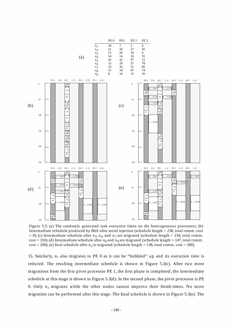
- 140 -

15. Similarly, n7 also migrates to PE 0 as it can be “bubbled” up and its execution time is

reduced. The resulting intermediate schedule is shown in Figure 5.3(c). After two more

migrations from the first pivot processor PE 1, the first phase is completed; the intermediate

schedule at this stage is shown in Figure 5.3(d). In the second phase, the pivot processor is PE

0. Only n3 migrates while the other nodes cannot improve their finish-times. No more

migration can be performed after this stage. The final schedule is shown in Figure 5.3(e). The

(a)

39 7 2 621 50 57 5615 28 39 654 14 16 5545 42 97 1215 20 57 7833 43 51 6051 18 47 748 16 15 20

n1n2n3n4n5n6n7n8n9

PE 0 PE1 PE 2 PE 3

(d)

n17

PE 0

n2

50

n5

42

n916

n3

28

n7

43

n414

0

50

100

150

200

n818

n620

L 01 L 12 L 23 L 30PE 1 PE 2 PE 3

250

n17

PE 0

n2

50

n5

42

n916

n315

n7

33

n416

0

50

100

150

200

n818

n620

L 01 L 12 L 23 L 30PE 1 PE 2 PE 3

250

3 → 8 (10)

3 ← 1(10) 1 → 4 (10)

8 ← 4 (10)

7 → 9 (60)

(b) (c)

Figure 5.3: (a) The randomly generated task execution times on the heterogeneous processors; (b)Intermediate schedule produced by BSA after serial injection (schedule length = 238, total comm. cost= 0); (c) Intermediate schedule after n3, n4, and n7 are migrated (schedule length = 218, total comm.cost = 110); (d) Intermediate schedule after n8 and n9 are migrated (schedule length = 147, total comm.cost = 200); (e) final schedule after n3 is migrated (schedule length = 138, total comm. cost = 200).

(e)

n17

PE 0

n2

50

n5

42

n98

n315

n7

33

n416

0

50

100

150

n8

47

n6

20

L 01 L 12 L 23 L 30PE 1 PE 2 PE 3

3 → 8 (10)

3 ← 1(10) 1 → 4 (10)

3 → 8 (10)

8 → 9 (50)9 ← 6 (50)

8 → 9 (50)

n17

PE 0

n2

50

n5

42

n98

n36

n7

33

n416

0

50

100

150

n8

47n620

L 01 L 12 L 23 L 30PE 1 PE 2 PE 3

8 ← 3(10)

3 ← 1(10) 1 → 4 (10)

8 → 9 (50)9 ← 6 (50) 8 → 9 (50)

3 ← 1(10)

7 ← 2 (10)

7 ← 2 (10)7 ←2 (10)

- 141 -

schedule length is only 138 which is considerably smaller than that for homogeneous

processors.

Next the task graph is scheduled to the same heterogeneous processors using the PBSA

algorithm with 3 PPEs (physical processors). According to the CPN-Dominant sequence, the

task graph is partitioned into 3 sets: , , and , as shown in

Figure 5.4. The estimated finish-times and target processors of the remote parent nodes

(RPNs) are shown in Figure 5.4(c). Note that according to the partitioning, only 6 nodes are

RPNs, namely, n1, n2, n3, n4, n6 and n7. The value of the importance factor is taken to be .

The EPFTs of the nodes n1, n2 and n6 are equal to their respective LPFTs because these nodes

occupy the earliest positions in the CPN-Dominant sequence. The EFTs of these nodes are

thus equal to the EPFTs independent of . Indeed, their EFTs are “accurate” with reference to

the schedules shown in Figure 5.3. Also their ETPEs are all chosen to be PE 1, the target

processor which gives the shortest CP length. On the other hand, the EPFTs of the nodes n3, n4

and n7 are equal to the sum of computation costs of the path from n1. The LPFTs of these

nodes are larger than their EPFTs because they are preceded by the more important nodes n1,

n1 n2 n6, ,{ } n7 n3 n4, ,{ } n8 n9 n5, ,{ }

(b)

n17

n2

50

n5

42

n9

16

n3

28

n7

43

n4

14

0

50

100

150

200

n8

18

n6

20

250

1st Partition

2nd Partition

3rd Partition

LPF

T(n

1)=

7

LPF

T(n

2)=

57

(c)

Figure 5.4: (a) Computations of the EPFTs of the RPNs n1, n2, n3, n4, n6and n7 based on the processing times for PE 1; (b) Computations ofthe LPFTs of the RPNs; (c) The estimated values of the RPNs.

EPFT(n1)=7

EPFT(n2)=57

EPST(n7)=100

n1

7

n2

50

n5

42

n9

n3

28

n7

43

n4

14

n8

18

n6

20

10

60

100

10

1010

1040

10

10

50

50

16

EPFT(n4)=21EPFT(n3)

=12

EPFT(n6)=77

(a)

RPN EPFT LPFT EFT ETPEn1 7 7 7 PE 1n2 57 57 57 PE 1n3 12 148 80 PE 3n4 21 162 91 PE 2n6 77 77 77 PE 1n7 100 120 110 PE 1

LPF

T(n

6)=

77

LPF

T(n

7)=

120

LPF

T(n

3)=

148

LPF

T(n

4)=

162

α 0.5

α

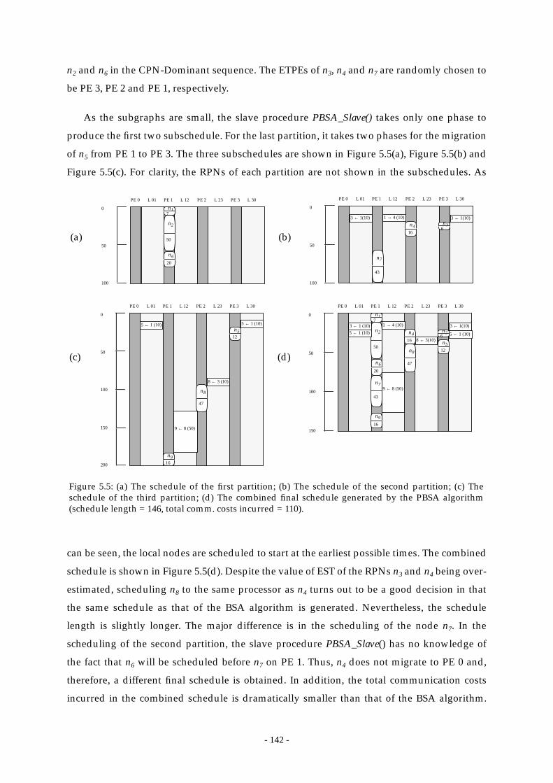
- 142 -

n2 and n6 in the CPN-Dominant sequence. The ETPEs of n3, n4 and n7 are randomly chosen to

be PE 3, PE 2 and PE 1, respectively.

As the subgraphs are small, the slave procedure PBSA_Slave() takes only one phase to

produce the first two subschedule. For the last partition, it takes two phases for the migration

of n5 from PE 1 to PE 3. The three subschedules are shown in Figure 5.5(a), Figure 5.5(b) and

Figure 5.5(c). For clarity, the RPNs of each partition are not shown in the subschedules. As

can be seen, the local nodes are scheduled to start at the earliest possible times. The combined

schedule is shown in Figure 5.5(d). Despite the value of EST of the RPNs n3 and n4 being over-

estimated, scheduling n8 to the same processor as n4 turns out to be a good decision in that

the same schedule as that of the BSA algorithm is generated. Nevertheless, the schedule

length is slightly longer. The major difference is in the scheduling of the node n7. In the

scheduling of the second partition, the slave procedure PBSA_Slave() has no knowledge of

the fact that n6 will be scheduled before n7 on PE 1. Thus, n4 does not migrate to PE 0 and,

therefore, a different final schedule is obtained. In addition, the total communication costs

incurred in the combined schedule is dramatically smaller than that of the BSA algorithm.

(a)

(c)

Figure 5.5: (a) The schedule of the first partition; (b) The schedule of the second partition; (c) Theschedule of the third partition; (d) The combined final schedule generated by the PBSA algorithm(schedule length = 146, total comm. costs incurred = 110).

(b)

(d)

n17

PE 0

n2

50

0

50

100

n620

L 01 L 12 L 23 L 30PE 1 PE 2 PE 3 PE 0

n36

n7

43

n416

0

50

100

L 01 L 12 L 23 L 30PE 1 PE 2 PE 3

3 ← 1(10) 1 → 4 (10)

PE 0

n512

n916

0

50

100

150

n8

47

L 01 L 12 L 23 L 30PE 1 PE 2 PE 3

5 ← 1 (10)

3 ← 1(10)

5 ← 1 (10)

200

8 ← 3 (10)

9 ← 8 (50)

n17

PE 0

n2

50n5

12

n9

16

n36

n7

43

n416

0

50

100

150

n8

47n6

20

L 01 L 12 L 23 L 30PE 1 PE 2 PE 3

8 ← 3(10)

3 ← 1 (10) 1 → 4 (10)

9 ← 8 (50)

3 ← 1(10)5 ← 1 (10) 5 ← 1 (10)

- 143 -

The large difference is due to the fact that in the BSA algorithm, nodes do not migrate to other

target processors if their start-times do not improve. However, the slave procedure of the

PBSA algorithm does not have this global knowledge about the intermediate state of the

schedule, and thus it attempts to locally schedule every node to start at the earliest possible

times.


In this section, we present the performance results of the PBSA algorithm and make

comparisons with the MH, DLS, and BU algorithms. Since the MH, DLS, and BU algorithms

are sequential, we also compare their performance with our serialized PBSA algorithm—the

BSA algorithm. We also compare the solution quality and efficiency of the PBSA and BSA

algorithms and examine the trade-off between two performance measures: solution quality

and running time.

For testing the algorithms, we generated two suites of task graphs: The first suite

consisted of regular graphs and the second suite consisted of irregular graphs. The regular

graphs represent various parallel applications including Gaussian elimination [189],

Cholesky factorization [130], and FFT [130]. Since these applications operate on matrices, the

number of nodes (and edges) in their task graphs depends on the size of the data matrix. The

number of nodes in the task graph for each application is roughly O(N2) where N is the size of

the matrix; this is about the same for all applications. The suite of random task graphs

consisted of graphs with arbitrary structures.

Within each type of graph, we chose 3 values of CCR (0.1, 1.0, and 10.0). The weights on

the nodes and edges were generated randomly such that the average value of CCR

corresponded to 0.1, 1.0 or 10.0. A value of CCR equal to 0.1 represents a computation-

intensive task graph (or coarse granularity), a value of 10.0 represents a communication-

intensive task graph (or fine granularity), and a value of 1.0 represents a graph in which

computation and communication are just about balanced.

We used four target system topologies: an 8-node hypercube, a 4x2 mesh, an 8-node fully

connected network, and an 8-node random topology. These target systems are assumed to be

composed of homogeneous processors.

The algorithms were implemented on an Intel Paragon/XP-S; the sequential algorithms

(MH, DLS, BU, and BSA) were executed on a single processor of the Paragon, an i860/XP.

The PBSA algorithm was executed on 2, 4, 8, and 16 processors.

- 144 -

In our first experiment, we compared the schedules produced by the BSA algorithm and

the PBSA algorithm (16 Paragon processors) with those of the MH, DLS and BU algorithms

for Cholesky factorization task graphs of various size. The results of Table 5.1 show

comparisons for three different values of CCR on four network topologies. The entries of the

table show the ratios of the schedule length generated by the MH, DLS, BU and PBSA

algorithms, to those of the BSA algorithm.

From this table we make a number of observations. First, the BSA algorithm outperforms

the MH, DLS, and BU algorithms since all ratios are greater than 1. Second, the margin of

improvement is different for each algorithm: the largest margin is over the BU algorithm (up

to 43%); the minimum margin is over the MH algorithm. This also implies that MH is better

Table 5.1: Ratios of schedule lengths generated by the MH, DLS, BU and PBSA (using16 PPEs) algorithms for Cholesky factorization task graphs on four target topologies.

MatrixSize

CCR = 0.1

MH DLS BU PBSABSA BSA BSA BSA

CCR = 1.0 CCR = 10.0

19242934394449545964

1.106 1.144 1.180 1.1511.105 1.160 1.183 1.1511.094 1.159 1.200 1.1521.106 1.154 1.203 1.1431.111 1.165 1.201 1.1471.100 1.147 1.171 1.1511.104 1.141 1.192 1.1501.112 1.150 1.201 1.1501.109 1.143 1.182 1.1431.114 1.151 1.190 1.145

19242934394449545964

19242934394449545964

19242934394449545964

8-nodehypercube

4x2mesh

8-nodefullyconnected

8-noderandom

Topology

1.146 1.204 1.261 1.1681.143 1.216 1.278 1.1701.134 1.208 1.273 1.1661.136 1.224 1.252 1.1711.138 1.198 1.265 1.1651.151 1.198 1.279 1.1621.137 1.232 1.276 1.1631.139 1.198 1.272 1.1681.135 1.225 1.248 1.1691.150 1.230 1.263 1.167

1.106 1.128 1.196 1.1171.105 1.143 1.199 1.1151.094 1.142 1.218 1.1121.106 1.138 1.221 1.1171.111 1.148 1.219 1.1181.100 1.131 1.186 1.1161.104 1.126 1.209 1.1181.112 1.134 1.219 1.1121.109 1.127 1.198 1.1151.114 1.135 1.207 1.114

1.146 1.182 1.284 1.1381.143 1.193 1.302 1.1301.134 1.186 1.297 1.1291.136 1.199 1.274 1.1371.138 1.177 1.288 1.1371.151 1.177 1.304 1.1291.137 1.207 1.300 1.1321.139 1.176 1.296 1.1341.135 1.201 1.270 1.1351.150 1.205 1.287 1.132

1.186 1.260 1.332 1.1871.185 1.279 1.359 1.1891.173 1.269 1.353 1.1861.176 1.289 1.326 1.1851.178 1.257 1.342 1.1861.194 1.257 1.360 1.1911.177 1.299 1.357 1.1841.179 1.257 1.352 1.1891.175 1.291 1.321 1.1831.193 1.297 1.340 1.188

1.186 1.250 1.340 1.1581.192 1.266 1.366 1.1601.200 1.259 1.366 1.1571.189 1.230 1.368 1.1581.195 1.269 1.350 1.1531.194 1.249 1.381 1.1561.194 1.268 1.396 1.1581.185 1.237 1.371 1.1601.205 1.241 1.397 1.1611.177 1.252 1.405 1.153

1.072 1.089 1.116 1.0841.072 1.099 1.118 1.0901.064 1.099 1.129 1.0921.072 1.096 1.131 1.0881.076 1.103 1.130 1.0911.068 1.091 1.110 1.0891.071 1.088 1.123 1.0831.076 1.093 1.129 1.0901.074 1.089 1.117 1.0861.078 1.094 1.123 1.084

1.099 1.127 1.168 1.1071.097 1.135 1.179 1.1041.091 1.129 1.176 1.1031.093 1.139 1.162 1.1041.094 1.123 1.171 1.1061.102 1.123 1.180 1.1091.093 1.144 1.178 1.1071.094 1.123 1.175 1.1061.092 1.140 1.160 1.1041.102 1.143 1.170 1.099

1.126 1.174 1.202 1.1291.130 1.185 1.216 1.1271.136 1.181 1.217 1.1271.128 1.160 1.218 1.1281.133 1.188 1.207 1.1271.132 1.173 1.226 1.1331.132 1.187 1.234 1.1291.126 1.165 1.219 1.1311.139 1.168 1.235 1.1261.120 1.175 1.240 1.134

1.123 1.165 1.224 1.1391.119 1.172 1.235 1.1431.111 1.165 1.230 1.1421.113 1.177 1.212 1.1471.114 1.157 1.224 1.1391.125 1.157 1.235 1.1481.113 1.184 1.232 1.1421.115 1.157 1.229 1.1391.112 1.179 1.209 1.1481.124 1.182 1.222 1.141

1.169 1.227 1.307 1.1671.166 1.240 1.327 1.1711.155 1.231 1.321 1.1651.158 1.248 1.296 1.1711.160 1.220 1.312 1.1641.175 1.220 1.328 1.1661.159 1.257 1.325 1.1651.161 1.219 1.320 1.1701.157 1.250 1.292 1.1711.174 1.255 1.310 1.165

1.215 1.310 1.368 1.1961.222 1.331 1.396 1.1941.232 1.322 1.396 1.1951.219 1.286 1.398 1.1941.226 1.334 1.378 1.1911.225 1.309 1.413 1.1931.225 1.333 1.428 1.1911.215 1.294 1.401 1.1941.238 1.299 1.430 1.1911.206 1.313 1.438 1.195



- 145 -

than DLS, and DLS is better than BU. Third, the margin of improvement is larger when the

value of CCR is large. Fourth, the margin of improvement is also large when the target

system is an 8-node random network. Fifth, PBSA (using 16 PPEs) performs comparably to

MH, DLS, and BU algorithm when CCR was small but outperforms them when CCR was

large.

These observations are explicable by the following arguments: The scheduling

mechanism of the PBSA algorithm, due to its correct ordering of tasks through CPN-

Dominate sequence, is better than the strategies used by other algorithms. The poor

performance of the BU algorithm is primarily due to its strategy of evenly distributing the

tasks to the processors. The MH and DLS algorithms perform relatively better than BU

because they minimize the start-times of nodes. Furthermore, while the BU, DLS, and MH

algorithms rely on routing tables, the PBSA algorithm uses a more adaptive and efficient

approach by incrementally scheduling messages. Using a routing table does not optimize the

utilization of the communication links in that some links are contended by several messages

while some links are idle. This in turn delays the start-times of nodes. Finally PBSA generates

slightly degraded solutions compared with serial BSA in that PBSA relies on estimated

information.

We carried out the same experiments for the Gaussian elimination and FFT graphs. The

results of these experiments are presented in Table 5.2 and Table 5.3, respectively. An

inspection of Table 5.2 reveals that the serial BSA algorithm again performs better than the

MH, DLS, and BU algorithms in all cases. The PBSA algorithm performs better than these

algorithms when CCR is 1 or 10. The margin of improvement is even better when compared

to the previous case. Conclusions arrived at from the remaining results concur with the

observations made in the previous case. While the task graphs for Gaussian elimination and

Cholesky factorization share some similarities, the task graph for FFT is quite different (hence

different matrix size are used). The results, however, again indicate that the BSA algorithm is

better than all three other algorithms. Based on the results of these experiments, the BSA

algorithm is better than the other three algorithms in general when CCR is low but yields

significant improvement when CCR is high.

Our next experiment was for the random graphs, the results of which are shown in Table

5.4. The number of nodes was varied from 200 to 2000 with increments of 200. These very

large graphs can lead to a more consistent performance without a particular bias towards a

particular algorithm. As indicated by the values shown in Table 5.4, the performance

improvement yielded by BSA is more significant in this case (25 to 66% improvement over

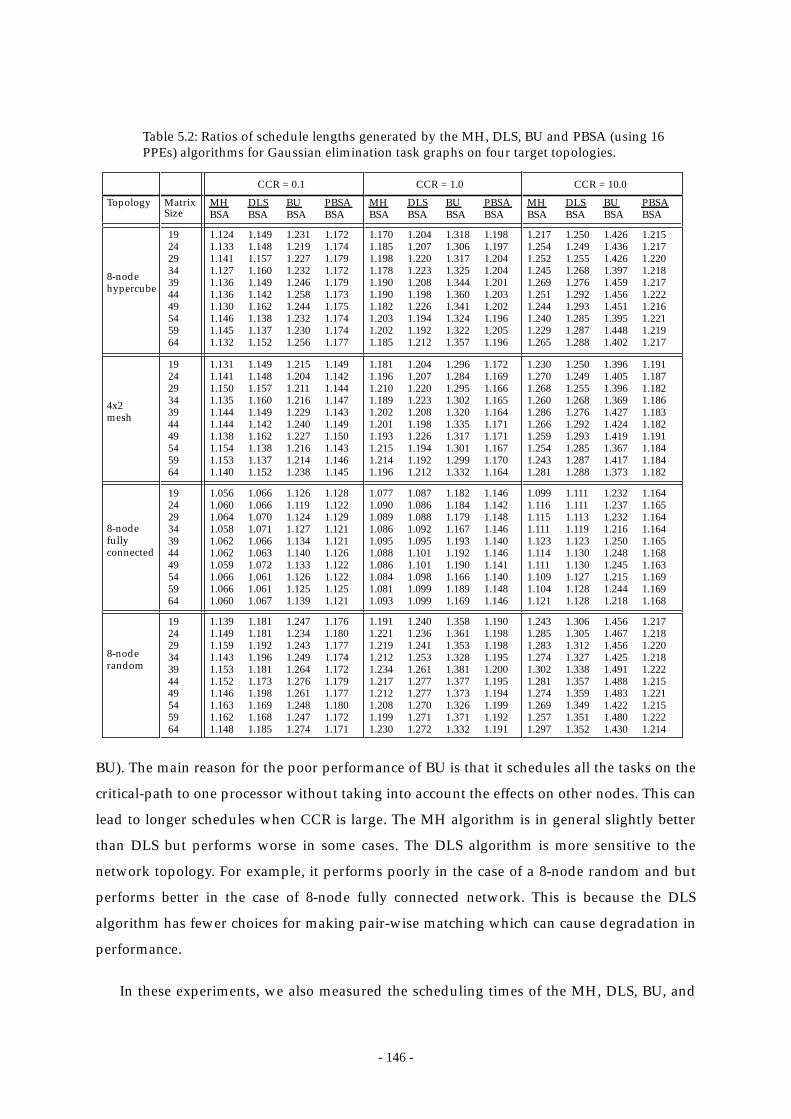
- 146 -

BU). The main reason for the poor performance of BU is that it schedules all the tasks on the

critical-path to one processor without taking into account the effects on other nodes. This can

lead to longer schedules when CCR is large. The MH algorithm is in general slightly better

than DLS but performs worse in some cases. The DLS algorithm is more sensitive to the

network topology. For example, it performs poorly in the case of a 8-node random and but

performs better in the case of 8-node fully connected network. This is because the DLS

algorithm has fewer choices for making pair-wise matching which can cause degradation in

performance.

In these experiments, we also measured the scheduling times of the MH, DLS, BU, and

Table 5.2: Ratios of schedule lengths generated by the MH, DLS, BU and PBSA (using 16PPEs) algorithms for Gaussian elimination task graphs on four target topologies.

MatrixSize

CCR = 0.1


CCR = 1.0 CCR = 10.0

19242934394449545964

1.124 1.149 1.231 1.1721.133 1.148 1.219 1.1741.141 1.157 1.227 1.1791.127 1.160 1.232 1.1721.136 1.149 1.246 1.1791.136 1.142 1.258 1.1731.130 1.162 1.244 1.1751.146 1.138 1.232 1.1741.145 1.137 1.230 1.1741.132 1.152 1.256 1.177

19242934394449545964

19242934394449545964

19242934394449545964

8-nodehypercube

4x2mesh


8-noderandom

Topology

1.170 1.204 1.318 1.1981.185 1.207 1.306 1.1971.198 1.220 1.317 1.2041.178 1.223 1.325 1.2041.190 1.208 1.344 1.2011.190 1.198 1.360 1.2031.182 1.226 1.341 1.2021.203 1.194 1.324 1.1961.202 1.192 1.322 1.2051.185 1.212 1.357 1.196

1.131 1.149 1.215 1.1491.141 1.148 1.204 1.1421.150 1.157 1.211 1.1441.135 1.160 1.216 1.1471.144 1.149 1.229 1.1431.144 1.142 1.240 1.1491.138 1.162 1.227 1.1501.154 1.138 1.216 1.1431.153 1.137 1.214 1.1461.140 1.152 1.238 1.145

1.181 1.204 1.296 1.1721.196 1.207 1.284 1.1691.210 1.220 1.295 1.1661.189 1.223 1.302 1.1651.202 1.208 1.320 1.1641.201 1.198 1.335 1.1711.193 1.226 1.317 1.1711.215 1.194 1.301 1.1671.214 1.192 1.299 1.1701.196 1.212 1.332 1.164

1.217 1.250 1.426 1.2151.254 1.249 1.436 1.2171.252 1.255 1.426 1.2201.245 1.268 1.397 1.2181.269 1.276 1.459 1.2171.251 1.292 1.456 1.2221.244 1.293 1.451 1.2161.240 1.285 1.395 1.2211.229 1.287 1.448 1.2191.265 1.288 1.402 1.217

1.230 1.250 1.396 1.1911.270 1.249 1.405 1.1871.268 1.255 1.396 1.1821.260 1.268 1.369 1.1861.286 1.276 1.427 1.1831.266 1.292 1.424 1.1821.259 1.293 1.419 1.1911.254 1.285 1.367 1.1841.243 1.287 1.417 1.1841.281 1.288 1.373 1.182

1.056 1.066 1.126 1.1281.060 1.066 1.119 1.1221.064 1.070 1.124 1.1291.058 1.071 1.127 1.1211.062 1.066 1.134 1.1211.062 1.063 1.140 1.1261.059 1.072 1.133 1.1221.066 1.061 1.126 1.1221.066 1.061 1.125 1.1251.060 1.067 1.139 1.121

1.077 1.087 1.182 1.1461.090 1.086 1.184 1.1421.089 1.088 1.179 1.1481.086 1.092 1.167 1.1461.095 1.095 1.193 1.1401.088 1.101 1.192 1.1461.086 1.101 1.190 1.1411.084 1.098 1.166 1.1401.081 1.099 1.189 1.1481.093 1.099 1.169 1.146

1.099 1.111 1.232 1.1641.116 1.111 1.237 1.1651.115 1.113 1.232 1.1641.111 1.119 1.216 1.1641.123 1.123 1.250 1.1651.114 1.130 1.248 1.1681.111 1.130 1.245 1.1631.109 1.127 1.215 1.1691.104 1.128 1.244 1.1691.121 1.128 1.218 1.168

1.139 1.181 1.247 1.1761.149 1.181 1.234 1.1801.159 1.192 1.243 1.1771.143 1.196 1.249 1.1741.153 1.181 1.264 1.1721.152 1.173 1.276 1.1791.146 1.198 1.261 1.1771.163 1.169 1.248 1.1801.162 1.168 1.247 1.1721.148 1.185 1.274 1.171

1.191 1.240 1.358 1.1901.221 1.236 1.361 1.1981.219 1.241 1.353 1.1981.212 1.253 1.328 1.1951.234 1.261 1.381 1.2001.217 1.277 1.377 1.1951.212 1.277 1.373 1.1941.208 1.270 1.326 1.1991.199 1.271 1.371 1.1921.230 1.272 1.332 1.191

1.243 1.306 1.456 1.2171.285 1.305 1.467 1.2181.283 1.312 1.456 1.2201.274 1.327 1.425 1.2181.302 1.338 1.491 1.2221.281 1.357 1.488 1.2151.274 1.359 1.483 1.2211.269 1.349 1.422 1.2151.257 1.351 1.480 1.2221.297 1.352 1.430 1.214



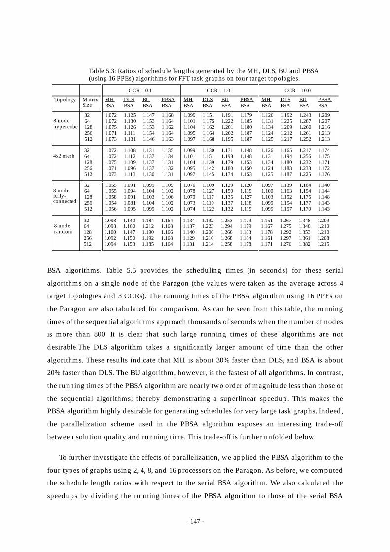
- 147 -

BSA algorithms. Table 5.5 provides the scheduling times (in seconds) for these serial

algorithms on a single node of the Paragon (the values were taken as the average across 4

target topologies and 3 CCRs). The running times of the PBSA algorithm using 16 PPEs on

the Paragon are also tabulated for comparison. As can be seen from this table, the running

times of the sequential algorithms approach thousands of seconds when the number of nodes

is more than 800. It is clear that such large running times of these algorithms are not

desirable.The DLS algorithm takes a significantly larger amount of time than the other

algorithms. These results indicate that MH is about 30% faster than DLS, and BSA is about

20% faster than DLS. The BU algorithm, however, is the fastest of all algorithms. In contrast,

the running times of the PBSA algorithm are nearly two order of magnitude less than those of

the sequential algorithms; thereby demonstrating a superlinear speedup. This makes the

PBSA algorithm highly desirable for generating schedules for very large task graphs. Indeed,

the parallelization scheme used in the PBSA algorithm exposes an interesting trade-off

between solution quality and running time. This trade-off is further unfolded below.

To further investigate the effects of parallelization, we applied the PBSA algorithm to the

four types of graphs using 2, 4, 8, and 16 processors on the Paragon. As before, we computed

the schedule length ratios with respect to the serial BSA algorithm. We also calculated the

speedups by dividing the running times of the PBSA algorithm to those of the serial BSA

Table 5.3: Ratios of schedule lengths generated by the MH, DLS, BU and PBSA(using 16 PPEs) algorithms for FFT task graphs on four target topologies.

MatrixSize

CCR = 0.1


CCR = 1.0 CCR = 10.0

3264128256512

1.072 1.125 1.147 1.1681.072 1.130 1.153 1.1641.075 1.126 1.153 1.1621.071 1.111 1.154 1.1641.073 1.131 1.146 1.163

8-nodehypercube

Topology

1.099 1.151 1.191 1.1791.101 1.175 1.222 1.1851.104 1.162 1.201 1.1801.095 1.164 1.202 1.1871.097 1.168 1.195 1.187

1.126 1.192 1.243 1.2091.131 1.225 1.287 1.2071.134 1.209 1.260 1.2161.124 1.212 1.261 1.2131.125 1.217 1.252 1.213



3264128256512

1.072 1.108 1.131 1.1351.072 1.112 1.137 1.1341.075 1.109 1.137 1.1311.071 1.096 1.137 1.1321.073 1.113 1.130 1.131

4x2 mesh1.099 1.130 1.171 1.1481.101 1.151 1.198 1.1481.104 1.139 1.179 1.1531.095 1.142 1.180 1.1501.097 1.145 1.174 1.153

1.126 1.165 1.217 1.1741.131 1.194 1.256 1.1751.134 1.180 1.232 1.1711.124 1.183 1.233 1.1721.125 1.187 1.225 1.176

3264128256512

1.055 1.091 1.099 1.1091.055 1.094 1.104 1.1021.058 1.091 1.103 1.1061.054 1.081 1.104 1.1021.056 1.095 1.099 1.102

8-nodefully-connected

1.076 1.109 1.129 1.1201.078 1.127 1.150 1.1191.079 1.117 1.135 1.1271.073 1.119 1.137 1.1181.074 1.122 1.132 1.119

1.097 1.139 1.164 1.1401.100 1.163 1.194 1.1441.103 1.152 1.175 1.1481.095 1.154 1.177 1.1431.095 1.157 1.170 1.143

3264128256512

1.098 1.140 1.184 1.1641.098 1.160 1.212 1.1681.100 1.147 1.190 1.1661.092 1.150 1.192 1.1681.094 1.153 1.185 1.164

8-noderandom

1.134 1.192 1.253 1.1791.137 1.223 1.294 1.1791.140 1.206 1.266 1.1831.129 1.210 1.268 1.1841.131 1.214 1.258 1.178

1.151 1.267 1.348 1.2091.167 1.275 1.340 1.2101.178 1.292 1.353 1.2101.161 1.297 1.361 1.2081.171 1.276 1.382 1.215

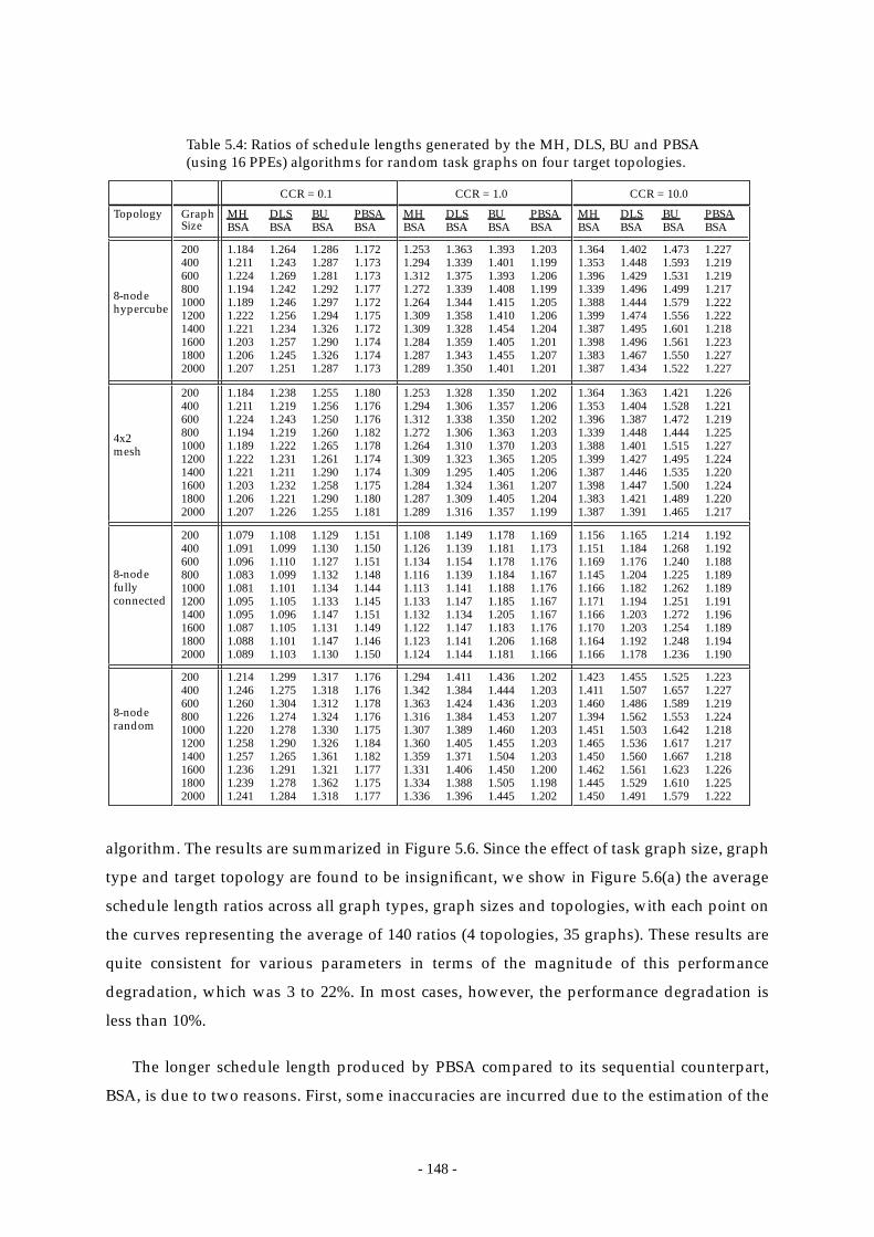
- 148 -

algorithm. The results are summarized in Figure 5.6. Since the effect of task graph size, graph

type and target topology are found to be insignificant, we show in Figure 5.6(a) the average

schedule length ratios across all graph types, graph sizes and topologies, with each point on

the curves representing the average of 140 ratios (4 topologies, 35 graphs). These results are

quite consistent for various parameters in terms of the magnitude of this performance

degradation, which was 3 to 22%. In most cases, however, the performance degradation is

less than 10%.

The longer schedule length produced by PBSA compared to its sequential counterpart,

BSA, is due to two reasons. First, some inaccuracies are incurred due to the estimation of the

Table 5.4: Ratios of schedule lengths generated by the MH, DLS, BU and PBSA(using 16 PPEs) algorithms for random task graphs on four target topologies.

GraphSize

CCR = 0.1


CCR = 1.0 CCR = 10.0

200400600800100012001400160018002000

1.184 1.264 1.286 1.1721.211 1.243 1.287 1.1731.224 1.269 1.281 1.1731.194 1.242 1.292 1.1771.189 1.246 1.297 1.1721.222 1.256 1.294 1.1751.221 1.234 1.326 1.1721.203 1.257 1.290 1.1741.206 1.245 1.326 1.1741.207 1.251 1.287 1.173

200400600800100012001400160018002000

200400600800100012001400160018002000

200400600800100012001400160018002000

8-nodehypercube

4x2mesh


8-noderandom

Topology

1.253 1.363 1.393 1.2031.294 1.339 1.401 1.1991.312 1.375 1.393 1.2061.272 1.339 1.408 1.1991.264 1.344 1.415 1.2051.309 1.358 1.410 1.2061.309 1.328 1.454 1.2041.284 1.359 1.405 1.2011.287 1.343 1.455 1.2071.289 1.350 1.401 1.201

1.184 1.238 1.255 1.1801.211 1.219 1.256 1.1761.224 1.243 1.250 1.1761.194 1.219 1.260 1.1821.189 1.222 1.265 1.1781.222 1.231 1.261 1.1741.221 1.211 1.290 1.1741.203 1.232 1.258 1.1751.206 1.221 1.290 1.1801.207 1.226 1.255 1.181

1.253 1.328 1.350 1.2021.294 1.306 1.357 1.2061.312 1.338 1.350 1.2021.272 1.306 1.363 1.2031.264 1.310 1.370 1.2031.309 1.323 1.365 1.2051.309 1.295 1.405 1.2061.284 1.324 1.361 1.2071.287 1.309 1.405 1.2041.289 1.316 1.357 1.199

1.364 1.402 1.473 1.2271.353 1.448 1.593 1.2191.396 1.429 1.531 1.2191.339 1.496 1.499 1.2171.388 1.444 1.579 1.2221.399 1.474 1.556 1.2221.387 1.495 1.601 1.2181.398 1.496 1.561 1.2231.383 1.467 1.550 1.2271.387 1.434 1.522 1.227

1.364 1.363 1.421 1.2261.353 1.404 1.528 1.2211.396 1.387 1.472 1.2191.339 1.448 1.444 1.2251.388 1.401 1.515 1.2271.399 1.427 1.495 1.2241.387 1.446 1.535 1.2201.398 1.447 1.500 1.2241.383 1.421 1.489 1.2201.387 1.391 1.465 1.217

1.079 1.108 1.129 1.1511.091 1.099 1.130 1.1501.096 1.110 1.127 1.1511.083 1.099 1.132 1.1481.081 1.101 1.134 1.1441.095 1.105 1.133 1.1451.095 1.096 1.147 1.1511.087 1.105 1.131 1.1491.088 1.101 1.147 1.1461.089 1.103 1.130 1.150

1.108 1.149 1.178 1.1691.126 1.139 1.181 1.1731.134 1.154 1.178 1.1761.116 1.139 1.184 1.1671.113 1.141 1.188 1.1761.133 1.147 1.185 1.1671.132 1.134 1.205 1.1671.122 1.147 1.183 1.1761.123 1.141 1.206 1.1681.124 1.144 1.181 1.166

1.156 1.165 1.214 1.1921.151 1.184 1.268 1.1921.169 1.176 1.240 1.1881.145 1.204 1.225 1.1891.166 1.182 1.262 1.1891.171 1.194 1.251 1.1911.166 1.203 1.272 1.1961.170 1.203 1.254 1.1891.164 1.192 1.248 1.1941.166 1.178 1.236 1.190

1.214 1.299 1.317 1.1761.246 1.275 1.318 1.1761.260 1.304 1.312 1.1781.226 1.274 1.324 1.1761.220 1.278 1.330 1.1751.258 1.290 1.326 1.1841.257 1.265 1.361 1.1821.236 1.291 1.321 1.1771.239 1.278 1.362 1.1751.241 1.284 1.318 1.177

1.294 1.411 1.436 1.2021.342 1.384 1.444 1.2031.363 1.424 1.436 1.2031.316 1.384 1.453 1.2071.307 1.389 1.460 1.2031.360 1.405 1.455 1.2031.359 1.371 1.504 1.2031.331 1.406 1.450 1.2001.334 1.388 1.505 1.1981.336 1.396 1.445 1.202

1.423 1.455 1.525 1.2231.411 1.507 1.657 1.2271.460 1.486 1.589 1.2191.394 1.562 1.553 1.2241.451 1.503 1.642 1.2181.465 1.536 1.617 1.2171.450 1.560 1.667 1.2181.462 1.561 1.623 1.2261.445 1.529 1.610 1.2251.450 1.491 1.579 1.222



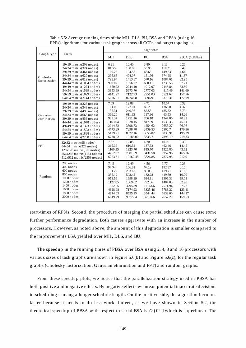
- 149 -

start-times of RPNs. Second, the procedure of merging the partial schedules can cause some

further performance degradation. Both causes aggravate with an increase in the number of

processors. However, as noted above, the amount of this degradation is smaller compared to

the improvements BSA yielded over MH, DLS, and BU.

The speedup in the running times of PBSA over BSA using 2, 4, 8 and 16 processors with

various sizes of task graphs are shown in Figure 5.6(b) and Figure 5.6(c), for the regular task

graphs (Cholesky factorization, Gaussian elimination and FFT) and random graphs.

From these speedup plots, we notice that the parallelization strategy used in PBSA has

both positive and negative effects. By negative effects we mean potential inaccurate decisions

in scheduling causing a longer schedule length. On the positive side, the algorithm becomes

faster because it needs to do less work. Indeed, as we have shown in Section 5.2, the

theoretical speedup of PBSA with respect to serial BSA is , which is superlinear. The

19x19 matrix(209 nodes)24x24 matrix(324 nodes)29x29 matrix(464 nodes)34x34 matrix(629 nodes)39x39 matrix(819 nodes)44x44 matrix(1034 nodes)49x49 matrix(1274 nodes)54x54 matrix(1539 nodes)59x59 matrix(1829 nodes)64x64 matrix(2144 nodes)

Table 5.5: Average running times of the MH, DLS, BU, BSA and PBSA (using 16PPEs) algorithms for various task graphs across all CCRs and target topologies.

6.21 10.40 3.80 8.13 0.2681.55 138.88 55.95 110.21 3.49109.25 194.55 66.65 149.63 4.64295.66 494.07 151.76 374.25 11.37793.94 1413.87 570.16 1087.61 32.95939.02 1556.77 660.11 1235.58 37.211650.72 2744.10 1012.97 2143.84 63.803853.99 5973.70 2777.03 4817.49 141.694141.27 7122.93 2951.03 5521.67 157.765036.51 8224.08 3096.91 6375.31 177.09

MH DLS BU BSA PBSA (16PPEs)

7.69 12.88 4.71 10.07 0.32101.00 172.01 69.29 136.50 4.37135.31 240.97 82.55 185.32 5.79366.20 611.93 187.96 463.53 14.26983.34 1751.16 706.18 1347.06 40.821163.04 1928.15 817.59 1530.33 45.012044.52 3398.73 1254.62 2655.27 76.964773.39 7398.78 3439.53 5966.74 170.965129.21 8822.16 3655.02 6838.91 195.396238.02 10186.00 3835.71 7896.19 219.33

Choleskyfactorization

Gaussianelimination

32x32 matrix(95 nodes)64x64 matrix(223 nodes)128x128 matrix(511 nodes)256x256 matrix(1151 nodes)512x512 matrix(2559 nodes)

7.67 12.85 4.70 10.05 0.33365.35 610.52 187.53 462.46 14.451160.35 1923.70 815.70 1526.80 43.624762.37 7381.69 3431.58 5952.96 165.366223.61 10162.48 3826.85 7877.95 212.91

200 nodes400 nodes600 nodes800 nodes1000 nodes1200 nodes1400 nodes1600 nodes1800 nodes2000 nodes

7.45 12.49 4.56 9.77 0.2397.94 166.81 67.19 132.37 3.15131.22 233.67 80.06 179.71 4.18355.12 593.42 182.28 449.50 10.70953.59 1698.19 684.81 1306.31 29.021127.85 1869.82 792.86 1484.03 32.981982.66 3295.89 1216.66 2574.94 57.224628.98 7174.93 3335.46 5786.22 123.114974.03 8555.25 3544.44 6632.00 144.176049.29 9877.84 3719.66 7657.29 159.53

19x19 matrix(228 nodes)24x24 matrix(348 nodes)29x29 matrix(493 nodes)34x34 matrix(663 nodes)39x39 matrix(858 nodes)44x44 matrix(1078 nodes)49x49 matrix(1323 nodes)54x54 matrix(1593 nodes)59x59 matrix(1888 nodes)64x64 matrix(2208 nodes)

FFT

Random

AlgorithmGraph type Sizes

O P2( )

- 150 -

plots indicate that the parallel PBSA, when run on 2 processors, is about 6 to 10 times faster

than the serial BSA. By using more PPEs, the speedup appears to increase almost linearly.

With 16 PPEs, the speedup is close to 50. The observed speedup, therefore, agrees with the

predicted superlinear speedup.

The substantial gain in speedup versus some degradation in performance implies that the

PBSA algorithm is scalable in both performance and speedup. Furthermore, it provides a

trade-off between performance and speed, and thus offers a choice of using a faster version

with some loss in performance or a slower version with better performance.

For comparison, in Figure 5.7, Figure 5.8, and Figure 5.9, we show the average schedule

length ratios and average speedups of the PBSA algorithm with respect to the MH, DLS, and

BU algorithms, respectively. First, we notice that the average schedule length ratios in these

plots are all less than 1, which implies that the overall performance of PBSA is better than

these three algorithms. Secondly, an interesting observation is that the average schedule

200 400 600 800 1000 1200 1400 1600 1800 20000

10

20

30

40

50


19 24 29 34 39 44 49 54 59 640

10

20

30

40


2 4 8 161

1.05

1.1

1.15

1.2

1.25

CCR=0.1CCR=1.0CCR=10.0

(b) Speedup for Regular Graphs.

(a) Schedule Length Ratios.

(c) Speedup for Random Graphs.

Figure 5.6: (a) Average schedule length ratios of the PBSA algorithm to the BSAalgorithm; (b) Average speedups of PBSA with respect to BSA for regulargraphs; (c) Average speedups of PBSA with respect to BSA for random graphs.

- 151 -

length ratios are smaller when CCR is larger; in contrast, in Figure 5.6, we notice that the

ratios increase with CCRs. This observation leads to a conclusion that the MH, DLS, and BU

algorithms are much more sensitive to the value of CCR, when compared with the PBSA

algorithm. This shows that although the PBSA algorithm relies on estimation, its core

incremental scheduling strategy is superior to the strategies used by the other three

algorithms. As to the speedups of PBSA with respect to these algorithms, we can see that the

speedups are superlinear even for the BU algorithm which is the fastest among the three.

One set of results using random task graphs (with sizes from 200 to 2000) on a 4x2 mesh

of heterogeneous processors are given in Table 5.6, which shows the average percentage

degradations in schedule lengths of PBSA with respect to those of BSA. We can see that the

average degradation is less than 20% in most cases.

We also performed experiments to study the effect of on the PBSA algorithm’s

performance. We varied from 0.1 to 0.9 with increments of 0.1. For each value of , we ran

2 4 8 160.8

0.85

0.9

0.95

1


200 400 600 800 1000 1200 1400 1600 1800 20000

5

10

15

20

25

30

35


19 24 29 34 39 44 49 54 59 640

5

10

15

20

25

30





Figure 5.7: (a) Average schedule length ratios of the PBSA algorithm tothe MH algorithm; (b) Average speedups of PBSA over MH for regulargraphs; (c) Average speedups of PBSA over MH for random graphs.

α

α α

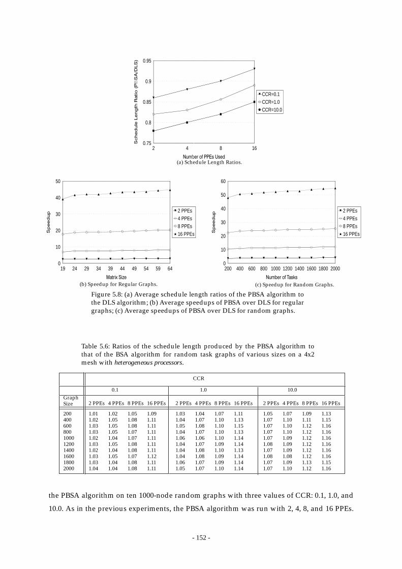
- 152 -

the PBSA algorithm on ten 1000-node random graphs with three values of CCR: 0.1, 1.0, and

10.0. As in the previous experiments, the PBSA algorithm was run with 2, 4, 8, and 16 PPEs.

2 4 8 160.75

0.8

0.85

0.9

0.95


200 400 600 800 1000 1200 1400 1600 1800 20000

10

20

30

40

50

60


19 24 29 34 39 44 49 54 59 640

10

20

30

40

50





Figure 5.8: (a) Average schedule length ratios of the PBSA algorithm tothe DLS algorithm; (b) Average speedups of PBSA over DLS for regulargraphs; (c) Average speedups of PBSA over DLS for random graphs.

200400600800100012001400160018002000

Table 5.6: Ratios of the schedule length produced by the PBSA algorithm tothat of the BSA algorithm for random task graphs of various sizes on a 4x2mesh with heterogeneous processors.

GraphSize

1.01 1.02 1.05 1.091.02 1.05 1.08 1.111.03 1.05 1.08 1.111.03 1.05 1.07 1.111.02 1.04 1.07 1.111.03 1.05 1.08 1.111.02 1.04 1.08 1.111.03 1.05 1.07 1.121.03 1.04 1.08 1.111.04 1.04 1.08 1.11

2 PPEs 4 PPEs 8 PPEs 16 PPEs

0.1

1.03 1.04 1.07 1.111.04 1.07 1.10 1.131.05 1.08 1.10 1.151.04 1.07 1.10 1.131.06 1.06 1.10 1.141.04 1.07 1.09 1.141.04 1.08 1.10 1.131.04 1.08 1.09 1.141.06 1.07 1.09 1.141.05 1.07 1.10 1.14


1.0

1.05 1.07 1.09 1.131.07 1.10 1.11 1.151.07 1.10 1.12 1.161.07 1.10 1.12 1.161.07 1.09 1.12 1.161.08 1.09 1.12 1.161.07 1.09 1.12 1.161.08 1.08 1.12 1.161.07 1.09 1.13 1.151.07 1.10 1.12 1.16


10.0

CCR

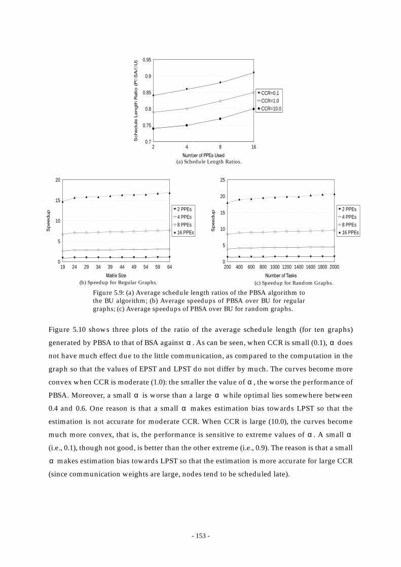
- 153 -

Figure 5.10 shows three plots of the ratio of the average schedule length (for ten graphs)

generated by PBSA to that of BSA against . As can be seen, when CCR is small (0.1), does

not have much effect due to the little communication, as compared to the computation in the

graph so that the values of EPST and LPST do not differ by much. The curves become more

convex when CCR is moderate (1.0): the smaller the value of , the worse the performance of

PBSA. Moreover, a small is worse than a large while optimal lies somewhere between

0.4 and 0.6. One reason is that a small makes estimation bias towards LPST so that the

estimation is not accurate for moderate CCR. When CCR is large (10.0), the curves become

much more convex, that is, the performance is sensitive to extreme values of . A small

(i.e., 0.1), though not good, is better than the other extreme (i.e., 0.9). The reason is that a small

makes estimation bias towards LPST so that the estimation is more accurate for large CCR

(since communication weights are large, nodes tend to be scheduled late).

2 4 8 160.7

0.75

0.8

0.85

0.9

0.95


200 400 600 800 1000 1200 1400 1600 1800 20000

5

10

15

20

25


19 24 29 34 39 44 49 54 59 640

5

10

15

20





Figure 5.9: (a) Average schedule length ratios of the PBSA algorithm tothe BU algorithm; (b) Average speedups of PBSA over BU for regulargraphs; (c) Average speedups of PBSA over BU for random graphs.

α α

α

α α

α

α α

α

- 154 -


In this chapter we have presented a parallel algorithm for scheduling in a general

distributed computing environment in that it accounts for more realistic considerations

including a limited number of processors, link contention, heterogeneity of processors and

the network topology. The major strength of the proposed PBSA algorithm lies in its

incremental strategy of scheduling nodes and messages together. It first uses the CPN-

Dominant sequence to serialize the task graph to one PE, and then allows the nodes to

migrate to other PEs for start-time improvements. In this manner, the start-times of the

nodes, and hence the schedule length, are reduced incrementally. Furthermore, in the course

of migration, the routing and scheduling of communication messages between tasks are also

optimized. As to parallelization of the algorithm, we partition the CPN-Dominant sequence

into disjoint portions so that each portion is scheduled independently. Using an effective

start-time estimation strategy, which does not incur high time-complexity, the PBSA

0.1 0.2 0.3 0.4 0.5 0.6 0.7 0.8 0.91

1.1

1.2

1.3

1.4

1.5

1.6


0.1 0.2 0.3 0.4 0.5 0.6 0.7 0.8 0.91

1.05

1.1

1.15

1.2

1.25

1.3


0.1 0.2 0.3 0.4 0.5 0.6 0.7 0.8 0.91

1.1

1.2

1.3

1.4

1.5

1.6


(a) CCR = 0.1

(c) CCR = 10.0

(b) CCR = 1.0

Figure 5.10: The effect of parameter on schedule length.α

- 155 -

algorithm can generate solutions with quality comparable to that generated by the sequential

BSA algorithm.

We have evaluated the PBSA algorithm using extensive variations of input parameters

including graph types, graph sizes, CCRs and target network topologies. Comparisons with

three other APN scheduling algorithms have also been made. Based on the experimental

results, we find that the PBSA algorithm can provide a short and scalable schedule, and is

useful for scheduling large task graphs, a virtually impossible task if using sequential

algorithms.

- 156 -

Chapter 6

Conclusions and Future Research

6.1 Summary

Scheduling tasks of a parallel program to the processors is one of the most crucial

components of a parallel processing environment. Since the scheduling problem is NP-

complete in general, solutions are generated using heuristics. However, most of the previous

heuristics are based on simplifying assumptions about the structure of the parallel program

and the target parallel architecture. Common simplifying assumptions include uniform task

execution times, zero inter-task communication times, contention-free communication, full

connectivity of parallel processors and the availability of an unlimited number of processors.

These assumptions, which are not valid in practical situations, restrict the applicability of the

heuristics.

To be applicable in a practical environment, a scheduling algorithm needs to address a

number of important issues. On the one hand, it must exploit parallelism by identifying the

task graph structure, and take into consideration task granularity, load balancing, arbitrary

task weights and communication costs, the number of target processors available, and the

scheduling of inter-processor communication. To give good performance while taking into

account all these aspects can produce a scheduling algorithm with very high time-

complexity. In order to be of practical use, the running time of a scheduling algorithm must

remain within a reasonable range. These two conflicting requirements make the design of an

efficient scheduling algorithm more intricate and challenging.

We have developed a number of scheduling algorithms that meet the conflicting goals of

high-performance and low time-complexity, by taking into account the important details of

the application and machine. A distinctive feature of our research is that the proposed

algorithms are parallel and can be executed on a parallel machine. Parallelization further

reduces the time-complexity and thus allows the scheduling of large applications. No prior

work on the parallelization of scheduling algorithms have been reported.

- 157 -

In summary, we have addressed four essential issues in the design of efficient scheduling

algorithms: performance, time-complexity, scalability, and applicability.

In the first place, the proposed algorithms provide high-performance implying that they

provide high quality solutions. The algorithms are also robust in that they can tackle the

problem under a wide range of input parameters (e.g., the number of target processors

available, diverse task graph structures, etc.). While the proposed algorithms are heuristic in

nature, their performance is superior to contemporary heuristics in general, as observed

through an extensive experimentation.

Secondly, the time-complexity of the algorithm is of prime importance insofar as the

quality of the solutions is not compromised. We have accomplished to maintain low

complexities of the algorithms by using efficient methodologies and then by parallelizing the

scheduling algorithms. The rationale of parallelization is that parallel processing is realized

only when there is a parallel processing platform, which can be utilized not only to speed up

the scheduling process further but also to improve the solution quality.

The applicability of a scheduling algorithm is also enhanced through parallelization. For

example, a parallel machine using a parallel scheduling algorithm could “self-schedule” its

own programs using multiple processors. Also, with the advanced networking and

communication tools, integrated environments using both parallel machines and network of

workstations are becoming increasingly popular. In such an environment (see Figure 1.1(d) in

Chapter 1) a parallel machine could execute a fast parallel scheduling algorithm to schedule

tasks on multiple heterogeneous workstations.

Thirdly, the proposed scheduling algorithms are scalable, that is, the algorithms give

consistent good performance even when presented with large input (e.g., a 5000-node graph).

This is important because, in practice, a task graph generated from a numerical application

can easily have a few thousands nodes.

Finally, the proposed algorithms are useful in practical situations in that the algorithms

consider realistic assumptions about the program and multiprocessor models. An algorithm

based on simplifying assumptions may not be useful in practical compile-time scheduling

even if it is shown to give good performance in simulation studies. As such, our proposed

scheduling algorithms are based on realistic assumptions such as arbitrary computation and

communication weights, link contention, and processor network topology. Consequently, the

proposed algorithms are applicable to a variety of parallel and distributed platforms.

Moreover, the algorithms generates high quality solutions when they are evaluated using real

- 158 -

benchmarks generated by a parallel program compiler [10].

In summary, we have proposed three parallel algorithms for scheduling under different

environments: the PFAST (Parallel Fast Assignment using Search Technique), the PGS

(Parallel Genetic Scheduling) algorithm, and the PBSA (Parallel Bubble Scheduling and

Allocation) algorithm.

6.1.1 A Low Time-Complexity Algorithm

The time-complexity of an algorithm and its solution quality are in general conflicting

goals in the design of efficient scheduling algorithms. Our previous study indicates that not

only does the quality of existing algorithms differ considerably but their running times can

vary by large margins [9]. The proposed PFAST algorithm is designed to take linear-time to

generate solutions with high quality. The PFAST algorithm first constructs an initial schedule

quickly in linear-time and then refines it by using multiple physical processors, each of which

operates on a disjoint subset of blocking-nodes as a search neighborhood. The physical

processors communicate periodically to exchange the best solution found thus far. As the

number of search steps required is a small constant which is independent of the size of the

input DAG, the algorithm effectively takes linear-time to determine the final schedule.

In our study, we have compared the sequential FAST algorithm with a number of well-

known efficient scheduling algorithms. The FAST algorithm has been shown to be better than

the other algorithms in terms of both solution quality and running time. Since the algorithm

takes linear-time, it is the fastest algorithm to our knowledge. In our experiments using

random task graphs for which optimal solutions are known, the PFAST algorithm generates

optimal solutions for a significant portion of all the test cases, and close-to-optimal solutions

for the remaining cases. The PFAST algorithm also exhibits good scalability in that it gives a

consistent performance when applied to large task graphs. An interesting finding of the

PFAST algorithm is that parallelization can sometimes improve its solution quality. This is

due to the partitioning of the blocking-nodes set, which implies a partitioning of the search

neighborhood. The partitioning allows the algorithm to explore the search space

simultaneously, thereby enhancing the likelihood of getting better solutions.

6.1.2 Scheduling using Parallel Genetic Search

Genetic algorithms use global search techniques to explore different regions of the search

space simultaneously by keeping track of a set of potential solutions of diverse

characteristics, called a population. As such, genetic search algorithms are widely reckoned

- 159 -

as effective techniques in solving numerous optimization problems because they can

potentially locate better solutions at the expense of longer running time. Another merit of

genetic search is that its inherent parallelism can be exploited to further reduce its running

time. Thus, a parallel genetic search technique in scheduling is a viable approach in

producing high quality solutions using short running times.

We have proposed a parallel genetic algorithm for scheduling, called the PGS algorithm,

using a novel encoding scheme, an effective initial population generation strategy, and

computationally efficient genetic search operators. The major motivation of using a genetic

search approach is that the recombinative nature of a genetic algorithm can potentially

determine an optimal scheduling list leading to an optimal schedule. As such, we encode a

scheduling list (i.e., a topological ordering of the input DAG) as a genetic string. Instead of

generating the initial population totally randomly, we generate the initial set of strings based

on a number of effective scheduling lists such as ALAP list, b-level list, t-level list, etc. We use a

novel crossover operator, which is a variant of the order crossover operator, in the scheduling

context. The proposed crossover operator has the potential to effectively combine the good

characteristics of two parent strings in order to generate a scheduling string which can lead to

a schedule with shorter schedule length. The crossover operator is easy to implement and is

computationally efficient.

In our experimental studies, we have found that the PGS algorithm generates optimal

solutions for more than half of all the cases in which random task graphs were used. In

addition, the PGS algorithm demonstrates an almost linear speedup and is therefore scalable.

While the DCP algorithm has already been shown to outperform many leading algorithms,

the PGS algorithm is even better since it generates solutions with comparable quality while

using significantly less time due to its effective parallelization. The PGS algorithm

outperforms the well-known DSC algorithm in terms of both the solution quality and

running time. An extra advantage of the PGS algorithm is scalability: by using more parallel

processors, the algorithm can be used for scheduling larger task graphs.

6.1.3 A Parallel Algorithm for Scheduling under RealisticEnvironments

The proposed PBSA algorithm is for APN scheduling in that it is based on considerations

such as a limited number of processors, link contention, heterogeneity of processors, and

processor network topology. As a result, the algorithm is useful for distributed systems

including clusters of workstations. The major strength of the proposed PBSA algorithm lies in

its incremental strategy of scheduling nodes and messages together. It first uses the CPN-

- 160 -

Dominant sequence to serialize the task graph to one PE, and then allows the nodes to

migrate to other PEs for improving their start-times. In this manner, the start-times of the

nodes, and hence, the schedule length, are optimized incrementally. Furthermore, in the

course of migration, the routing and scheduling of communication messages between tasks

are also optimized. The PBSA algorithm first partitions the input DAG into a number of

disjoint subgraphs. The subgraphs are then scheduled independently in multiple physical

processors, each of which runs a sequential BSA algorithm. The final schedule is constructed

by concatenating the subschedules produced. The proposed algorithm is, therefore, the first

attempt of its kind in that it is a parallel algorithm and it also solves the scheduling problem

by considering all the important scheduling parameters.

We have evaluated the BSA and PBSA algorithms by testing them in experiments using

extensive variations of input parameters including graph types, graph sizes, CCRs, and

target network topologies. Comparisons with three other APN scheduling algorithms have

also been made. Based on the experimental results, we find that the PBSA algorithm can

provide a scalable schedule, and can be useful for scheduling large task graphs which are

virtually impossible to schedule using sequential algorithms.

6.2 Future Research Directions

The research described in this thesis can be extended in several directions. One of the

most challenging direction is to extend the current work to heterogeneous computing platforms.

Heterogeneous computing (HC) using physically distributed diverse machines connected via

a high-speed network for solving complex applications is likely to dominate the next era of

high-performance computing. One class of a HC environment is a suite of sequential

machines known as a network of workstations (NOWs). Another class, known as the

distributed heterogeneous supercomputing system (DHSS), is a suite of machines comprising

a variety of sequential and parallel computers—providing an even higher level of

parallelism. In general, it is impossible for a single machine architecture with its associated

compiler, operating system, and programming tools to satisfy all the computational

requirements in an application equally well. However, a heterogeneous computing

environment that consists of a heterogeneous suite of machines, high-speed interconnections,

interfaces, operating systems, communication protocols and programming environments

provides a variety of architectural capabilities, which can be orchestrated to perform an

application that has diverse execution requirements. Due to the latest advances in

networking technologies, HC is likely to flourish in the near future.

- 161 -

The goal of HC, be it a NOW or a DHSS, is to achieve the minimum completion time for

an application. A challenging future research is to design efficient algorithms for scheduling

and mapping of applications to the machines in a HC environment. Task-to-machine

mapping in a HC environment is beyond doubt more complicated than in a homogeneous

environment. In a HC environment, a computation can be decomposed into tasks, each of

which may have substantially different processing requirements. For example a signal

processing task may strictly require a machine possessing DSP processing capability. While

the PBSA algorithm proposed in this research is a first step toward this direction, more work

is needed. One possible research direction is to first devise a new model of heterogeneous

parallel applications as well as new models of HC environments. Based on these new models,

more optimized algorithms can be designed.

Another avenue of further research is to extend the applicability of the proposed PFAST

and PGS algorithms. While they are targeted to be used in BNP scheduling, the algorithms

may be extended to handle APN scheduling as well. However, some novel efficient

algorithmic techniques for scheduling messages to links need to be sought lest the time-

complexity of the algorithms increase. On the other hand, further improvement of the PFAST

algorithm may be accomplished by using some low time-complexity algorithmic techniques

to track the actual blocking-nodes set dynamically.

Finally, the PGS algorithm has shown an encouraging performance. Further

improvements may be possible if we can determine an optimal set of control parameters,

including crossover rate, mutation rate, population size, number of generations, and number

of parallel processors used. However, finding an optimal parameters set for a particular

genetic algorithm is hitherto an open research problem.

- 162 -

References

[1] T.L. Adam, K.M. Chandy, and J. Dickson, “A Comparison of List Scheduling for ParallelProcessing Systems,” Communications of the ACM, vol. 17, Dec. 1974, pp. 685-690.

[2] I. Ahmad and M.K. Dhodhi, “Task Assignment using a Problem-Space GeneticAlgorithm,” Concurrency: Practice and Experience, vol. 7 (5), Aug. 1995, pp. 411-428.

[3] I. Ahmad and A. Ghafoor, “Semi-distributed Load Balancing for Massively ParallelMulticomputer Systems,” IEEE Transactions on Software Engineering, vol. 17, no. 10, Oct.1991, pp. 987-1004.

[4] I. Ahmad and Y.-K. Kwok, “A New Approach to Scheduling Parallel Programs UsingTask Duplication,” Proceedings of the 23rd International Conference on Parallel Processing,vol. II, Aug. 1994, pp. 47-51.

[5] —, “A Parallel Approach to Multiprocessor Scheduling,” Proceedings of the 9thInternational Parallel Processing Symposium, Apr. 1995, pp. 289-293.

[6] —, “On Exploiting Task Duplication in Parallel Program Scheduling,” submitted to IEEETransactions on Parallel and Distributed Systems.

[7] —, “A Parallel Algorithm for Scheduling Parallel Tasks,” submitted to IEEE Transactionson Parallel and Distributed Systems.

[8] I. Ahmad, Y.-K. Kwok, and M.-Y. Wu, “Performance Comparison of Algorithms forStatic Scheduling of DAGs to Multiprocessors,” Proceedings of the 2nd AustralianConference on Parallel and Real-Time Systems, Sep. 1995, pp. 185-192.

[9] —, “Analysis, Evaluation, and Comparison of Algorithms for Scheduling Task Graphson Parallel Processors,“ International Symposium on Parallel Architectures, Algorithms, andNetworks, Beijing, China, Jun. 1996, pp. 207-213.

[10] I. Ahmad, Y.-K. Kwok, M.-Y. Wu, and W. Shu, “CASCH: A Software Tool for AutomaticParallelization and Scheduling of Programs on Multiprocessors,” submitted to IEEEConcurrency.

[11] H.H. Ali and H. El-Rewini, “The time complexity of scheduling interval orders withcommunication is polynomial,” Parallel Processing Letters, vol. 3, no. 1, 1993, pp. 53-58.

[12] S. Ali, S.M. Sait, and M.S.T. Benten, “GSA: Scheduling and Allocation using GeneticAlgorithm,” Proceedings of EURO-DAC’94, 1994, pp. 84-89.

[13] M.A. Al-Mouhamed, “Lower Bound on the Number of Processors and Time forScheduling Precedence Graphs with Communication Costs,” IEEE Transactions onSoftware Engineering, vol. 16, no. 12, Dec. 1990, pp. 1390-1401.

[14] V.A.F. Almeida, I.M. Vasconcelos, J.N.C. Arabe, and D.A. Menasce, “Using RandomTask Graphs to Investigate the Potential Benefits of Heterogeneity in Parallel Systems,”

- 163 -

Proceedings of Supercomputing‘92, 1992, pp. 683-691.

[15] G. Amdahl, “Validity of the Single Processor Approach to Achieving Large ScaleComputing Capability,” Proceedings of AFIPS Spring Joint Computer Conference 30,Reston, VA., 1967, pp. 483-485.

[16] F.D. Anger, J.J. Hwang, and Y.C. Chow, “Scheduling with sufficiently loosely coupledprocessors,” Journal of Parallel and Distributed Computing, 9, 1990, pp. 87-92.

[17] W. Atmar, “Notes on Simulation of Evolution,” IEEE Transactions on Neural Networks,vol. 5, no. 1, Jan. 1994, pp. 130-147.

[18] A.F. Bashir, V. Susarla, and K. Vairavan, “A Statistical Study of the Performance of aTask Scheduling Algorithm,” IEEE Transactions on Computers, vol. C-32, no. 8, Aug. 1983,pp. 774-777.

[19] J. Baxter and J.H. Patel, “The LAST Algorithm: A Heuristic-Based Static Task AllocationAlgorithm,” Proceedings of International Conference on Parallel Processing, vol. II, Aug.1989, pp. 217-222.

[20] M. Beck, K.K. Pingali, and A. Nicolau, “Static scheduling for dynamic dataflowmachines,” Journal of Parallel and Distributed Computing, 10, 1990, pp. 279-288.

[21] M.S.T. Benten and S.M. Sait, “Genetic Scheduling of Task Graphs,” International Journalof Electronics, vol. 77, no. 4, Oct. 1994, pp. 401-415.

[22] J. Blazewicz, M. Drabowski, and J. Weglarz, “Scheduling Multiprocessor Tasks toMinimize Schedule length,” IEEE Transactions on Computers, vol. C-35, no. 5, May 1986,p. 389-393.

[23] J. Blazewicz, J. Weglarz, and M. Drabowski, “Scheduling Independent 2-processorTasks to Minimize Schedule Length,” Information Processing Letters, 18, 1984, pp. 267-273.

[24] S.H. Bokhari, “Dual Processor Scheduling with Dynamic Reassignment,” IEEETransactions on Software Engineering, vol. SE-5, no. 4, Jul. 1979, pp. 341-349.

[25] —, “On the Mapping Problem”, IEEE Transactions on Computers, vol. C-30, 1981, pp. 207-214.

[26] —, “A Shortest Tree Algorithm for Optimal Assignments Across Space and Time in aDistributed Systems,” IEEE Transactions on Software Engineering, vol. SE-7, no. 6, Nov.1981, pp. 583-589.

[27] —, “A Network Flow Model for Load Balancing in Circuit-Switched Multicomputers,”IEEE Transactions on Parallel and Distributed Systems, vol. 4, no. 6, pp. 649-657, Jun. 1993.

[28] N.S. Bowen, C.N. Nikolaou, and A. Ghafoor, “On the Assignment Problem of ArbitraryProcess Systems to Heterogeneous Distributed Computer Systems,” IEEE Transactionson Computers, vol. 41, no. 3, Mar. 1992, pp. 257-273.

[29] G. Bozoki and J.P. Richard, “A Branch-and-Bound Algorithm for Continuous-process

- 164 -

Task Shop Scheduling Problem,” AIIE Transactions, 2, 1970, pp. 246-252.

[30] J. Bruno, E.G. Coffman, and R. Sethi, “Scheduling Independent Tasks to Reduce MeanFinishing Time,”, Communications of the ACM, vol. 17, no. 7, Jul. 1974, pp. 382-387.

[31] T.L. Casavant and J.G. Kuhl, “A Taxonomy of Scheduling in General-PurposeDistributed Computing Systems,” IEEE Transactions on Software Engineering, vol. 14, no.2, Feb. 1988, pp. 141-154.

[32] R. Chandrasekharam, S. Subhramanian, and S. Chaudhury, “Genetic Algorithm forNode Partitioning Problem and Applications in VLSI Design,” IEE Proceedings, vol. 140,no. 5, Sep. 1993, pp. 255-260.

[33] G. Chen and T.H. Lai, “Scheduling Independent Jobs on Hypercubes,” Proceedings ofConference on Theoretical Aspects of Computer Science, 1988, pp. 273-280.

[34] —, “Preemptive Scheduling of Independent Jobs on a Hypercube,” InformationProcessing Letters, 28, 1988, pp. 201-206.

[35] H. Chen, B. Shirazi, and J. Marquis, “Performance Evaluation of A Novel SchedulingMethod: Linear Clustering with Task Duplication,” Proceedings of InternationalConference on Parallel and Distributed Systems, Dec. 1993, pp. 270-275.

[36] R. Cheng, M. Gen, and Y. Tsujimura, “A Tutorial Survey of Job-Shop SchedulingProblems using Genetic Algorithms. I. Representation,” Computers and IndustrialEngineering, vol. 30, no. 4, Sep. 1986, pp. 983-997.

[37] P. Chretienne, “A Polynomial Algorithm to Optimally Schedule Tasks on a VirtualDistributed System under Tree-like Precedence Constraints”, European Journal ofOperational Research, 43, 1989, pp. 225-230.

[38] W.W. Chu, M.-T. Lan, and J. Hellerstein, “Estimation of Intermodule Communication(IMC) and Its Applications in Distributed Processing Systems,” IEEE Transactions onComputers, vol. C-33, no. 8, Aug. 1984, pp. 691-699.

[39] Y.C. Chung and S. Ranka, “Application and Performance Analysis of a Compile-TimeOptimization Approach for List Scheduling Algorithms on Distributed-MemoryMultiprocessors,” Proceedings of Supercomputing’92, Nov. 1992, pp. 512-521.

[40] E.G. Coffman, Computer and Job-Shop Scheduling Theory, Wiley, New York, 1976.

[41] E.G. Coffman and R.L. Graham, “Optimal Scheduling for Two-Processor Systems,” ActaInformatica, vol. 1, 1972, pp. 200-213.

[42] J.Y. Colin and P. Chretienne, “C.P.M. Scheduling with Small Computation Delays andTask Duplication,” Operations Research, 1991, pp. 680-684.

[43] W.J. Dally, “Virtual-channel Flow Control,” IEEE Transactions on Parallel and DistributedSystems, vol. 3, Mar. 1992, pp. 194-205.

[44] S. Darbha and D.P. Agrawal, “A Fast and Scalable Scheduling Algorithm for Distributed

- 165 -

Memory Systems,” Proceedings of Symposium of Parallel and Distributed Processing, Oct.1995, pp. 60-63.

[45] L.D. Davis (Ed.), The Handbook of Genetic Algorithms, New York, Van Nostrand Reinhold,1991.

[46] M.K. Dhodhi, Imtiaz Ahmad, and Ishfaq Ahmad, “A Multiprocessor SchedulingScheme using Problem-Space Genetic Algorithms,” Proceedings of IEEE InternationalConference on Evolutionary Computation, 1995, vol. 1, pp. 214-219.

[47] V.A. Dixit-Radiya and D.K. Panda, “Task Assignment on Distributed-Memory Systemswith Adaptive Wormhole Routing,” Proceedings of International Symposium of Paralleland Distributed Systems, Dec. 1993, pp. 674-681.

[48] J. Du and J.Y.T. Leung, “Complexity of Scheduling Parallel Task Systems,” SIAM Journalon Discrete Mathematics, vol. 2, no. 4, Nov. 1989, pp. 473-487.

[49] R. Duncan, “A Survey of Parallel Computer Architectures,” IEEE Computer, Feb. 1990,pp. 5-16.

[50] H. El-Rewini and T.G. Lewis, “Scheduling Parallel Programs onto Arbitrary TargetMachines,” Journal of Parallel and Distributed Computing, vol. 9, no. 2, Jun. 1990, pp. 138-153.

[51] H. El-Rewini, H.H. Ali, and T.G. Lewis, “Task Scheduling in Multiprocessing Systems,”IEEE Computer, Dec. 1995, pp. 27-37.

[52] H. El-Rewini, T.G. Lewis, and H.H. Ali, Task Scheduling in Parallel and DistributedSystems, Prentice Hall, Englewood Cliffs, 1994.

[53] H. El-Rewini and H.H. Ali, “Static scheduling of conditional branches in parallelprograms,” Journal of Parallel and Distributed Computing, 24, 1995, pp. 41-54.

[54] M.D. Ercegovac, “Heterogeneity in Supercomputer Architectures,” Parallel Computing,7, 1988, pp. 367-372.

[55] E.B. Fernadez and B. Bussell, “Bounds on the Number of Processors and Time forMultiprocessor Optimal Schedules,” IEEE Transactions on Computers, vol. C-22, no. 8,Aug. 1973, pp. 745-751.

[56] J.L.R. Filho, P.C. Treleaven, and C. Alippi, “Genetic-Algorithm ProgrammingEnvironments,” IEEE Computer, Jun. 1994, pp. 28-43.

[57] P.C. Fishburn, Interval Orders and Interval Graphs, John Wiley & Sons, New York, 1985.

[58] S. Forrest and M. Mitchell, “What Makes a Problem Hard for a Genetic Algorithm? SomeAnomalous Results and Their Explanation,” Machine Learning, 13, 1993, pp. 285-319.

[59] R.F. Freund and H.J. Siegel, “Heterogeneous Processing,” IEEE Computer, Jun. 1993, pp.13-17.

- 166 -

[60] D.K. Friesen, “Tighter Bounds for LPT Scheduling on Uniform Processors,” SIAMJournal on Computing, vol. 16, no. 3, Jun. 1987, pp. 554-560.

[61] M. Fujii, T. Kasami, and K. Ninomiya, “Optimal Sequencing of Two EquivalentProcessors,” SIAM Journal Applied Mathematics, 17, no. 1, 1969.

[62] H. Gabow, “An almost linear algorithm for two-processor scheduling,” Journal of theACM, 29, 3, 1982, pp. 766-780.

[63] M.R. Garey and D.S. Johnson, Computers and Intractability: A Guide to the Theory of NP-Completeness, W.H. Freeman and Company, 1979.

[64] M.R. Garey, D. Johnson, R. Tarjan, and M. Yannakakis, “Scheduling opposing forests,”SIAM Journal on Algebraic Discrete Methods, 4, 1, 1983, pp. 72-92.

[65] D.D. Gajski and J. Peir, “Essential Issues in Multiprocessors,” IEEE Computer, 18, 6, Jun.1985.

[66] A. Gerasoulis and T. Yang, “A Comparison of Clustering Heuristics for SchedulingDAG’s on Multiprocessors,” Journal of Parallel and Distributed Computing, vol. 16, no. 4,Dec. 1992, pp. 276-291.

[67] —, “On the Granularity and Clustering of Directed Acyclic Task Graphs,” IEEETransactions on Parallel and Distributed Systems, vol. 4, no. 6, Jun. 1993, pp. 686-701.

[68] D. Ghosal, G. Serazzi, and S.K. Tripathi, “Processor Working Sets and its Use inScheduling Multiprocessor Systems,” IEEE Transactions on Software Engineering, May1991.

[69] M.A.C. Gill and A.Y. Zomaya, “Genetic Algorithms for Robotic Control,” Proceedingsof 1995 IEEE International Conference on Evolutionary Computation, vol. 1, pp. 462-466.

[70] C.A. Glass, C.N. Potts, and P. Shade, “Unrelated Parallel Machine Scheduling usingLocal Search,” Mathematical and Computer Modelling, vol. 20, no. 2, Jul. 1994, pp. 41-52.

[71] F. Glover, “Tabu Search—Part I,” ORSA Journal on Computing, vol. 1, no. 3, Summer1989, pp. 190-206.

[72] —, “Tabu Search—Part II,” ORSA Journal on Computing, vol. 2, no. 1, Winter 1990, pp. 4-32.

[73] D.E. Goldberg, Genetic Algorithms in Search, Optimization and Machine Learning, Addison-Wesley, Reading, Mass., 1989.

[74] M.J. Gonzalez, Jr., “Deterministic Processor Scheduling,” ACM Computing Surveys, vol.9, no. 3, Sep. 1977, pp. 173-204.

[75] T. Gonzales and S. Sahni, “Preemptive scheduling of uniform processor systems,”Journal of the ACM, 25, 1978, pp. 92-101.

[76] V.S. Gordon and D. Whitley, “A Machine-Independent Analysis of Parallel Genetic

- 167 -

Algorithms,” Complex Systems, vol. 8, no. 3, Jun. 1994, pp. 181-214.

[77] R.L. Graham, “Bounds for Certain Multiprocessing Anomalies,” Bell System TechnicalJournal, 45, 1966, pp. 1563-1581.

[78] R.L. Graham, E.L. Lawler, J.K. Lenstra, and A.H.G. Rinnoy Kan, “Optimization andApproximation in Deterministic Sequencing and Scheduling: A Survey,” Annals ofDiscrete Mathematics, no. 5, 1979, pp. 287-326.

[79] J.J. Grefenstette, “Optimization of Control Parameters for Genetic Algorithms,” IEEETransactions on Systems, Man, and Cybernetics, vol. SMC-16, no. 1, Jan./Feb. 1986, pp. 122-128.

[80] F. Gruau, G.R. Joubert, F.J. Peters, D. Trystram, and D.J. Evans, “The Mixed ParallelGenetic Algorithm,” Parallel Computing: Trends and Applications (Proc. of the InternationalConference ParCo’93), 1994, pp. 521-524.

[81] J. Gu, “Local Search for the Satisfiability (SAT) Problem,” IEEE Transactions on Systemsand Cybernetics, vol. 23, no. 3, Jul./Aug. 1993, pp. 1108-1129.

[82] S. Ha and E.A. Lee, “Compile-Time Scheduling and Assignment of Data-Flow ProgramGraphs with Data-Dependent Iteration,” IEEE Transactions on Computers, vol. 40, no. 11,Nov. 1991, pp. 1225-1238.

[83] M. Hanan and J. Kurtzberg, “A review of the placement and quadratic assignmentproblems,” SIAM Review, vol. 14, Apr. 1972, pp. 324-342.

[84] J.P. Hayes and T. Mudge, “Hypercube Supercomputers,” Proceedings of the IEEE, vol. 77,no. 12, Dec. 1989.

[85] D.S. Hochbaum and D.B. Shmoys, “Using Dual Approximation Algorithms forScheduling Problems: Theoretical and Practical Results,” Journal of the ACM, 34 (1), Jan.1987, pp. 144-162.

[86] —, “A Polynomial Approximation Scheme for Scheduling on Uniform Processors:Using the Dual Approximation Approach,” SIAM Journal on Computing, vol. 17, no. 3,Jun. 1988, pp. 539-551.

[87] J.H. Holland, Adaptation in Natural and Artificial Systems, University of Michigan Press,Ann Arbor, Mich., 1975.

[88] E.C. Horvath, S. Lam, and R. Sethi, “A level algorithm for preemptive scheduling,”Journal of the ACM, 24, 1977, pp. 32-43.

[89] E.S.H. Hou, N. Ansari, and H. Ren, “A Genetic Algorithm for MultiprocessorScheduling,” IEEE Transactions on Parallel and Distributed Systems, vol. 5, no. 2, Feb. 1994,pp. 113-120.

[90] T.C. Hu, “Parallel Sequencing and Assembly Line Problems,” Operations Research, vol.19, no. 6, Nov. 1961, pp. 841-848.

- 168 -

[91] C.L. Huntley and D.E. Brown, “Parallel Genetic Algorithms with Local Search,”Computers and Operations Research, vol. 23, no. 6, Jun. 1996, pp. 559-571.

[92] Kai Hwang, Advanced Computer Architecture: Parallelism, Scalability, Programmability,McGraw Hill, 1993.

[93] J.J. Hwang, Y.C. Chow, F.D. Anger, and C.Y. Lee, “Scheduling Precedence Graphs inSystems with Interprocessor Communication Times,” SIAM Journal on Computing, vol.18, no. 2, Apr. 1989, pp. 244-257.

[94] M.A. Iqbal, J.H. Saltz, and S.H. Bokhari, “A Comparative Analysis of Static andDynamic Load Balancing Strategies,” Proceedings of International Conference on ParallelProcessing, Aug. 1986, pp. 1040-1047.

[95] K.K. Jain and V. Rajaraman, “Lower and Upper Bounds on Time for MultiprocessorOptimal Schedules,” IEEE Transactions on Parallel and Distributed Systems, vol. 5, no. 8,Aug. 1994, pp. 879-886.

[96] —, “Improved Lower Bounds on Time and Processors for Scheduling PrecedenceGraphs on Multicomputer Systems,” Journal of Parallel and Distributed Computing, 28,1995, pp. 101-108.

[97] H. Jiang, L.N. Bhuyan, and D. Ghosal, “Approximate Analysis of Multiprocessing TaskGraphs,” Proceedings of International Conference on Parallel Processing, 1990, vol. III, pp.228-235.

[98] D.S. Johnson, C.H. Papadimitriou and M. Yannakakis, “How Easy Is Local Search,”Journal of Computer and System Sciences, vol. 37, no. 1, Aug. 1988, pp. 79-100.

[99] A. Kapsalis, G.D. Smith, V.J. Rayward-Smith, and T.C. Fogarty, “A Unified Paradigmfor Parallel Genetic Algorithms,” Evolutionary Computing, AISB Workshop (SelectedPapers), 1994, pp. 131-149.

[100] H. Kasahara and S. Narita, “Practical Multiprocessor Scheduling Algorithms forEfficient Parallel Processing,” IEEE Transactions on Computers, vol. C-33, Nov. 1984, pp.1023-1029.

[101] M. Kaufman, “An Almost-Optimal Algorithm for the Assembly Line SchedulingProblem,” IEEE Transactions on Computers, vol. C-23, no. 11, 1974, pp. 1169-1174.

[102] A.A. Khan, C.L. McCreary, and M.S. Jones, “A Comparison of MultiprocessorScheduling Heuristics,” Proceedings of International Conference on Parallel Processing, vol.II, Aug. 1994, pp. 243-250.

[103] W.H. Kohler and Steiglitz, “Characterization and theoretical comparison of branch-and-bound algorithms for permutation problems,” Journal of the ACM, vol. 21, Jan. 1974, pp.140-156.

[104] —, “A Preliminary Evaluation of the Critical Path Method for Scheduling Tasks onMultiprocessor Systems,” IEEE Transactions on Computers, Dec. 1975, pp. 1235-1238.

- 169 -

[105] S.J. Kim and J.C. Browne, “A General Approach to Mapping of Parallel Computationupon Multiprocessor Architectures,” Proceedings of International Conference on ParallelProcessing, vol. II, Aug. 1988, pp. 1-8.

[106] D. Kim and B.G. Yi, “A Two-Pass scheduling Algorithm for Parallel Programs,” ParallelComputing, 20, 1994, pp. 869-885.

[107] S. Kon’ya and T. Satoh, “Task Scheduling on a Hypercube with Link Contentions,”Proceedings of International Parallel Processing Symposium, Apr. 1993, pp. 363-368.

[108] B. Kruatrachue and T.G. Lewis, “Duplication Scheduling Heuristics (DSH): A NewPrecedence Task Scheduler for Parallel Processor Systems,” Technical Report, OregonState University, Corvallis, OR 97331, 1987.

[109] —, “Grain Size Determination for Parallel Processing,” IEEE Software, Jan. 1988, pp. 23-32.

[110] V. Kumar, A. Grama, A. Gupta, and G. Karypis, Introduction to Parallel Computing: Designand Analysis of Algorithms, The Benjamin/Cummings, 1994.

[111] Y.-K. Kwok, Efficient Algorithms for Scheduling and Mapping of Parallel Programs on ParallelArchitectures, M.Phil. Thesis, HKUST, Hong Kong, 1994.

[112] Y.-K. Kwok and I. Ahmad, “A Static Scheduling Algorithm Using Dynamic Critical Pathfor Assigning Parallel Algorithms Onto Multiprocessors,” Proceedings of InternationalConference on Parallel Processing, vol. II, Aug. 1994, pp. 155-159.

[113] —, “Bubble Scheduling: A Quasi Dynamic Algorithm for Static Allocation of Tasks toParallel Architectures,” Proceedings of the 7th Symposium on Parallel and DistributedProcessing, Oct. 1995, pp. 36-43.

[114] —, “Dynamic Critical-Path Scheduling: An Effective Technique for Allocating TaskGraphs onto Multiprocessors,” IEEE Transactions on Parallel and Distributed Systems, vol.7, no. 5, May 1996, pp. 506-521.

[115] —, “Bubble Scheduling: An Efficient Algorithm for Compile-Time Scheduling ofParallel Computations on Message Passing Architectures,” submitted for publication.

[116] —, “Efficient Scheduling of Arbitrary Task Graphs to Multiprocessors using A ParallelGenetic Algorithm,” submitted to Journal of Parallel and Distributed Computing.

[117] Y.-K. Kwok, I. Ahmad, and J. Gu, “FAST: A Low-Complexity Algorithm for EfficientScheduling of DAGs on Parallel Processors,” Proceedings of 25th International Conferenceon Parallel Processing, Aug. 1996, vol. II, pp. 150-157.

[118] Y.-K. Kwok, I. Ahmad, M. Kafil, and Imtiaz Ahmad, “Parallel Algorithms for OptimalScheduling of Arbitrary Task Graphs to Multiprocessors,” submitted for publication.

[119] Y.-K. Kwok, K. Karlapalem, I. Ahmad, and M.-P. Ng, “Design and Evaluation of DataAllocation Algorithms for Distributed Multimedia Database Systems,” IEEE Journal on

- 170 -

Selected Areas in Communications, vol. 14, no.7, Sep. 1996, pp. 1332-1348.

[120] B. Lee, A.R. Hurson, and T.Y. Feng, “A Vertically Layered Allocation Scheme for DataFlow Systems,” Journal of Parallel and Distributed Computing, vol. 11, 1991, pp. 175-187.

[121] S.Y. Lee and J.K. Aggarwal, “A Mapping Strategy for Parallel Processing,” IEEETransactions on Computers, vol. C-36, Apr. 1987, pp. 433-442.

[122] J.Y.-T. Leung and G.H. Young, “Minimizing Schedule Length subject to Minimum FlowTime,” SIAM Journal on Computing, vol. 18, no. 2, Apr. 1989, pp. 314-326.

[123] T.G. Lewis and H. El-Rewini, “Parallax: A Tool for Parallel Program Scheduling,” IEEEParallel and Distributed Technology, May 1993, vol. 1, no. 2, pp. 64-76.

[124] S.-C. Lin, W.F. Punch, and E.D. Goodman, “Coarse-Grain Parallel Genetic Algorithms:Categorization and New Approach,” Proceedings of the 6th International Symposium onParallel and Distributed Processing, 1994, pp. 28-37.

[125] J.-C. Liou and M.A. Palis, “An Efficient Task Clustering Heuristic for Scheduling DAGson Multiprocessors,” Workshop on Resource Management, Symposium of Parallel andDistributed Processing, 1996.

[126] —, “A Comparison of General Approaches to Multiprocessor Scheduling,” Proceedingsof 11th International Parallel Processing Symposium, Apr. 1997, pp. 152-156.

[127] D.C. Llewellyn, C. Tovey and M. Trick, “Local Optimization on Graphs,” DiscreteApplied Mathematics, vol. 23, no. 2, May 1989, pp. 157-178.

[128] V.M. Lo, “Temporal Communication Graphs: Lamport’s Process-Time GraphsAugmented for the Purpose of Mapping and Scheduling,” Journal of Parallel andDistributed Computing, 16, 1992, pp. 378-384.

[129] V.M. Lo, S. Rajopadhye, S. Gupta, D. Keldsen, M.A. Mohamed, B. Nitzberg, J.A. Telle,and X. Zhong, “OREGAMI: Tools for Mapping Parallel Computations to ParallelArchitectures,” Proceedings of International Journal of Parallel Programming, vol. 20, no. 3,1991, pp. 237-270.

[130] R.E. Lord, J.S. Kowalik, and S.P. Kumar, “Solving Linear Algebraic Equations on anMIMD Computer,” Journal of the ACM, 30(1), Jan. 1983, pp. 103-117.

[131] S. Manoharan and N.P. Topham, “An assessment of assignment schemes fordependency graphs,” Parallel Computing, 21, 1995, pp. 85-107.

[132] P. Markenscoff and Y.Y. Li, “Scheduling a Computational DAG on a Parallel Systemwith Communication Delays and Replication of Node Execution,” Proceedings ofInternational Parallel Processing Symposium, 1993, pp. 113-117.

[133] C. McCreary and H. Gill, “Automatic Determination of Grain Size of Efficient ParallelProcessing,” Communications of ACM, vol. 32, no. 9, Sep. 1989, pp. 1073-1078.

[134] C. McCreary, A.A. Khan, J.J. Thompson, and M.E. McArdle, “A Comparison of

- 171 -

Heuristics for Scheduling DAG’s on Multiprocessors,” Proceedings of InternationalParallel Processing Symposium, 1994, pp. 446-451.

[135] N. Mehdiratta and K. Ghose, “A Bottom-Up Approach to Task Scheduling onDistributed Memory Multiprocessor,” Proceedings of International Conference on ParallelProcessing, vol. II, Aug. 1994, pp. 151-154.

[136] D.A. Menasce and V.A.F. Almeida, “Cost-performance Analysis of Heterogeneity inSupercomputer Architectures,” Proceedings of ACM-IEEE Supercomputing’90, NewYork, 1990.

[137] D.A. Menasce and S.C. Porto, “Scheduling on Heterogeneous Message PassingArchitectures,” Journal of Computer and Software Engineering, 1, 3, 1993.

[138] D.A. Menasce, S.C. Porto, and S.K. Tripathi, “Static Heuristic Processor Assignment inHeterogeneous Message Passing Architectures,” International Journal of High SpeedComputing, 6, 1, Mar. 1994, pp. 115-137.

[139] —, “Processor Assignment in Heterogeneous Parallel Architectures,” Proceedings ofInternational Parallel Processing Symposium, 1992.

[140] D.A. Menasce, D. Saha, S.C. Porto, V.A.F. Almeida, and S.K. Tripathi, “Static andDynamic Processor Scheduling Disciplines in Heterogeneous Parallel Architectures,”Journal of Parallel and Distributed Computing, 28, 1995, pp. 1-18.

[141] H. Muhlenbein, “Parallel Genetic Algorithms, Population Genetics and CombinatorialOptimization,” Proceedings of International Conference on Genetic Algorithms, 1989, pp.416-421.

[142] —, “Evolution in Time and Space—The Parallel Genetic Algorithm,” Foundations ofGenetic Algorithms, 1991, pp. 316-337.

[143] J. Nang, “A Simple Parallelizing Scheme of Genetic Algorithm on Distributed-MemoryMultiprocessors,” International Journal of High Speed Computing, vol. 6, no. 3, Sep. 1994,pp. 451-474.

[144] T.M. Nabhan and A.Y. Zomaya, “A Parallel Simulated Annealing Algorithm with LowCommunication Overhead,” IEEE Transactions on Parallel and Distributed Systems, vol. 6,no. 12, Dec. 1995, pp. 1226-1233.

[145] M.A. Palis, J.-C. Liou, S. Rajasekaran, S. Shende and D.S.L. Wei, “Online Scheduling ofDynamic Trees,” Parallel Processing Letters, vol. 5, no. 4, Dec. 1995, pp. 635-646.

[146] M.A. Palis, J.-C. Liou, and D.S.L. Wei, “Task Clustering and Scheduling for DistributedMemory Parallel Architectures,” IEEE Transactions on Parallel and Distributed Systems,vol. 7, no. 1, Jan. 1996, pp. 46-55.

[147] S.S. Pande, D.P. Agrawal, and J. Mauney, “A Threshold Scheduling Strategy for Sisal onDistributed Memory Machines,” Journal of Parallel and Distributed Computing, 21, 1994,pp. 223-236.

- 172 -

[148] —, “A Scalable Scheduling Scheme for Functional Parallelism on Distributed MemoryMultiprocessor Systems,” IEEE Transactions on Parallel and Distributed Systems, vol. 6, no.4, Apr. 1995, pp. 388-399.

[149] C.H. Papadimitriou and K. Steiglitz, Combinatorial Optimization: Algorithms andComplexity, Prentice-Hall, Englewood Cliffs, NJ, 1982.

[150] C.H. Papadimitriou and J.D. Ullman, “A Communication-Time Tradeoff”, SIAM Journalon Computing, vol. 16, no. 4, Aug. 1987, pp. 639-646.

[151] C.H. Papadimitriou and M. Yannakakis, “Scheduling Interval-Ordered Tasks,” SIAMJournal on Computing, 8, 1979, pp. 405-409.

[152] —, “Towards an Architecture-Independent Analysis of Parallel Algorithms,” SIAMJournal on Computing, vol. 19, no. 2, Apr. 1990, pp. 322-328.

[153] D. Pease, A. Ghafoor, I. Ahmad, D.L. Andrews, K. Foudil-Bey, T.E. Karpinski, M.A.Mikki, and M. Zerrouki, “PAWS: A Performance Evaluation Tool for ParallelComputing Systems,” IEEE Computer, Jan. 1991, pp. 18-29.

[154] M. Prastein, Precedence-Constrained Scheduling with Minimum Time and Communication,M.S. Thesis, University of Illinois at Urbana-Champaign, 1987.

[155] M.J. Quinn, Parallel Computing: Theory and Practice, McGraw-Hill, 1994.

[156] C.V. Ramamoorthy, K.M. Chandy and M.J. Gonzalez, “Optimal Scheduling Strategiesin a Multiprocessor System,” IEEE Transactions on Computers, vol. C-21, Feb. 1972, pp.137-146.

[157] V.J. Rayward-Smith, “The Complexity of Preemptive Scheduling Given InterprocessorCommunication Delays,” Information Processing Letters, 25, 1987, pp. 123-125.

[158] —, “UET Scheduling with Unit Interprocessor Communication Delays,” Discrete AppliedMathematics, 18, 1987, pp. 55-71.

[159] M. Rebaudengo and M. Sonza Reorda, “An Experimental Analysis of the Effects ofMigration in Parallel Genetic Algorithms,” Proceedings of Euromicro Workshop onParallel and Distributed Processing, 1993, pp. 232-238.

[160] V. Sarkar, Partitioning and Scheduling Parallel Programs for Multiprocessors, MIT Press,Cambridge, MA, 1989.

[161] S. Selvakumar and C.S.R. Murthy, “Scheduling Precedence Constrained Task Graphswith Non-Negligible Intertask Communication onto Multiprocessors,” IEEETransactions on Parallel and Distributed Systems, vol. 5, no. 3, Mar. 1994, pp. 328-336.

[162] R. Sethi, “Scheduling Graphs on Two Processors,” SIAM Journal on Computing, vol. 5,no.1, Mar. 1976, pp. 73-82.

[163] M. Schwehm, T. Walter, B. Buchberger, and J. Volkert, “Mapping and Scheduling byGenetic Algorithms,” Proceedings of the 3rd Joint International Conference on Vector and

- 173 -

Parallel Processing (CONPAR’94), 1994, pp. 832-841.

[164] B. Shirazi, K. Kavi, A.R. Hurson, and P. Biswas, “PARSA: A Parallel ProgramScheduling and Assessment Environment,” Proceedings of International ConferenceParallel Processing, 1993, vol. II, pp. 68-72.

[165] B. Shirazi, M. Wang, and G. Pathak, “Analysis and Evaluation of Heuristic Methods forStatic Scheduling,” Journal of Parallel and Distributed Computing, no. 10, 1990, pp. 222-232.

[166] H.J. Siegel, Interconnection Networks for Large-Scale Parallel Processing: Theory and CaseStudies, 2nd Ed., McGraw-Hill, New York, 1990.

[167] H.J. Siegel, et al., “PASM: A Partitionable SIMD/MIMD System for Image Processingand Pattern Recognition,” IEEE Transactions on Computers, vol. C-30, no. 12, Dec. 1981,pp. 934-947.

[168] H.J. Siegel, et al., “Report of the Purdue Workshop on Grand Challenges in ComputerArchitectures for the Support of High Performance Computing,” Journal of Parallel andDistributed Computing, vol. 16, no. 3, Nov. 1992, pp. 199-211.

[169] H.J. Siegel, J.B. Armstrong and D.W. Watson, “Mapping Computer-Vision-RelatedTasks onto Reconfigurable Parallel Processing Systems,” IEEE Computer, Feb. 1992, pp.54-63.

[170] H.J. Siegel and C.B. Srunkel, “Inside Parallel Computers: Trends in InterconnectionNetworks,” IEEE Computational Science and Engineering, vol. 3, no. 3, Fall 1996, pp. 69-71.

[171] H.J. Siegel, H.G. Dietz, and J.K. Antonio, “Software Support for HeterogeneousComputing,” ACM Computing Surveys, vol. 28, no. 1, Mar. 1996, pp. 237-239.

[172] G.C. Sih and E.A. Lee, “A Compile-Time Scheduling Heuristic for Interconnection-Constrained Heterogeneous Processor Architectures,” IEEE Transactions on Parallel andDistributed Systems, vol. 4, no. 2, Feb. 1993, pp. 75-87.

[173] —, “Declustering: A new multiprocessor scheduling technique,” IEEE Transactions onParallel and Distributed Systems, vol. 4, no. 6, Jun. 1993, pp. 625-637.

[174] B.B. Simons and M.K. Warmuth, “A Fast Algorithm for Multiprocessor Scheduling ofunit-length jobs,” SIAM Journal on Computing, vol. 18, no. 4, Aug. 1989, pp. 690-710.

[175] M. Srinivas and L.M. Patnaik, “Adaptive Probabilities of Crossover and Mutation inGenetic Algorithms,” IEEE Transactions on Systems, Man and Cybernetics, vol. 24, no. 4,Apr. 1994, pp. 656-667.

[176] —, “Genetic Algorithms: A Survey,” IEEE Computer, Jun. 1994, pp. 17-26.

[177] H.S. Stone, “Multiprocessor Scheduling with the Aid of Network Flow Algorithms,”IEEE Transactions on Software Engineering, vol. SE-3, no. 1, Jan. 1977, pp. 85-93.

[178] R.T. Sumichrast, “Scheduling Parallel Processors to Minimize Setup Time,” Computersand Operations Research, vol. 14, no. 4, 1987, pp. 305-313.

- 174 -

[179] R.H. Storer, S.D. Wu, and R. Vaccari, “New Search Spaces for Sequencing Problems withApplication to Job Shop Scheduling,” Management Science, vol. 38, no. 10, Oct. 1992, pp.1495-1509.

[180] R. Tanese, “Parallel Genetic Algorithm for a Hypercube,” Proceedings of InternationalConference on Genetic Algorithms, 1987, pp. 177-183.

[181] —, “Distributed Genetic Algorithms,” Proceedings of International Conference on GeneticAlgorithms, 1989, pp. 434-439.

[182] D. Towsley, “Allocating Programs Containing Branches and Loops Within a MultipleProcessor System,” IEEE Transactions on Software Engineering, vol. SE-12, no. 10, Oct.1986, pp. 1018-1024.

[183] T.A. Varvarigou and V.P. Roychowdhury, “Scheduling in and out Forests in thePresence of Communication Delays,” Proceedings of International Parallel ProcessingSymposium, Apr. 1993, pp. 222-229.

[184] B. Veltman, B.J. Lageweg, and J.K. Lenstra, “Multiprocessor scheduling withcommunication delays,” Parallel Computing, 16, 1990, pp. 173-182.

[185] J. Ullman, “NP-Complete Scheduling Problems,” Journal of Computer and System Sciences,10, 1975, pp. 384-393.

[186] M.-F. Wang, “Message Routing Algorithms for Static Task Scheduling,” Proceedings ofthe 1990 Symposium on Applied Computing, 1990, pp. 276-281.

[187] Q. Wang and K.H. Cheng, “List scheduling of parallel task,” Information ProcessingLetters, 37, 1991, pp. 291-297.

[188] L. Wang, H.J. Siegel, and V.P. Roychowdhury, “A Genetic-Algorithm-Based Approachfor Task Matching and Scheduling in Heterogeneous Computing Environments,”Proceedings of 5th Heterogeneous Computing Workshop, 1996, pp. 72-85.

[189] W.S. Wong and R.J.T. Morris, “A New Approach to Choosing Initial Points in LocalSearch,” Information Processing Letters, vol. 30, no. 2, Jan. 1989, pp. 67-72.

[190] M.Y. Wu and D.D. Gajski, “Hypertool: A Programming Aid for Message-PassingSystems,” IEEE Transactions on Parallel and Distributed Systems, vol. 1, no. 3, Jul. 1990, pp.330-343.

[191] T. Yang and A. Gerasoulis, “List scheduling with and without communication delays,”Parallel Computing, 19, 1992, pp. 1321-1344.

[192] —, “PYRROS: Static Task Scheduling and Code Generation for Message PassingMultiprocessors,” Proceedings of 6th ACM International Conference on Supercomputing,1992, pp. 428-443.

[193] —, “DSC: Scheduling Parallel Tasks on an Unbounded Number of Processors,” IEEETransactions on Parallel and Distributed Systems, vol. 5, no. 9, Sep. 1994, pp. 951-967.

- 175 -

[194] C.-Q. Yang and B.P. Miller, “Critical Path Analysis for the Execution of Parallel andDistributed Programs,” Proceedings International Conference on Distributed ComputingSystems, Jun. 1988, pp. 366-373.

[195] J. Yang, L. Bic, and A. Nicolau, “A Mapping strategy for MIMD Computers,”International Journal of High Speed Computing, vol. 5, no. 1, 1993, pp. 89-103.

[196] Y. Zhu and C.L. McCreary, “Optimal and Near Optimal Tree Scheduling for ParallelSystems,” Proceedings of Symposium on Parallel and Distributed Processing, 1992, pp. 112-119.

- 176 -

Vita

October 7, 1968 Born in Hong Kong

November, 1991 B. Sc. (Eng.) in Computer Engineering, The University of

Hong Kong

November, 1994 M. Phil. in Computer Science, The Hong Kong University

of Science and Technology

1994—Present Ph.D. candidate, The Hong Kong University of Science

and Technology

Publications

Journal Articles:

[1] Y.-K. Kwok, K. Karlapalem, I. Ahmad, and M.P. Ng, “Design and Evaluation of DataAllocation Algorithms for Distributed Multimedia Database Systems,” IEEE Journal onSelected Area in Communications, vol. 14, no. 7, Sep. 1996, pp. 1332-1348.

[2] Y.-K. Kwok and I. Ahmad, “Dynamic Critical-Path Scheduling: An Effective Techniquefor Allocating Task Graphs to Multiprocessors,” IEEE Transactions on Parallel andDistributed Systems, vol. 7, no. 5, May 1996, pp. 506-521.

Articles in Refereed Conferences Proceedings:

[1] I. Ahmad, Y.-K. Kwok, M.-Y. Wu, and W. Shu, “Automatic Parallelization andScheduling of Programs on Multiprocessors using CASCH,” Proceedings of the 26thInternational Conference on Parallel Processing, Aug. 1997, to appear.

[2] Y.-K. Kwok and I. Ahmad, “A Parallel Genetic-Search-Based Algorithm for SchedulingArbitrary Task Graphs to Multiprocessors,” Proceedings of the 9th IASTED InternationalConference on Parallel and Distributed Computing and Systems, Oct. 1997, to appear.

[3] Y.-K. Kwok and I. Ahmad, “A Comparison of Task-Duplication-Based Algorithms forScheduling Parallel Programs to Message-Passing Systems,” Proceedings of the 11thInternational Symposium on High-Performance Computing (HPCS’97), 1997, to appear.

[4] I. Ahmad, Y.-K. Kwok, M.-Y. Wu, and W. Shu, “A Software Tool for AutomaticParallelization and Scheduling of Programs on Multiprocessors,” Proceedings of theEURO-PAR’97, Aug. 1997, to appear.

[5] K. Karlapalem, I. Ahmad, S.-K. So and Y.-K. Kwok, “Empirical Evaluation of DataAllocation Algorithms for Distributed Multimedia Database Systems,” Proceedings ofIEEE International Computer Software and Applications Conference (COMPSAC), 1997, toappear.

[6] Y.-K. Kwok, I. Ahmad, and J. Gu, “FAST: A Low Complexity Algorithm for Efficient

- 177 -

Scheduling of DAGs on Parallel Processors,” Proceedings of the 25th InternationalConference on Parallel Processing, Aug. 1996, pp. 150-157.

[7] I. Ahmad, Y.-K. Kwok, and M.-Y. Wu, “Analysis, Evaluation and Comparison ofAlgorithms for Scheduling Task Graphs to Parallel Processors,” Proceedings of the 1996International Symposium on Parallel Architecture, Algorithms and Networks, Beijing, China,Jun. 1996, pp. 207-213.

[8] Y.-K. Kwok and I. Ahmad, “Bubble Scheduling: A Quasi Dynamic Algorithm for StaticAllocation of Tasks to Parallel Architectures,” Proceedings of the 7th IEEE Symposium onParallel and Distributed Processing, Oct. 1995, pp. 36-43.

[9] I. Ahmad, Y.-K. Kwok and M.-Y. Wu, “Performance Comparison of Algorithms forStatic Scheduling of DAGs to Multiprocessors,” Proceedings of the 2nd AustralianConference on Parallel and Real-Time Systems, Sep. 1995, pp. 185-192.

[10] I. Ahmad and Y.-K. Kwok, “A Parallel Approach for Multiprocessor Scheduling,”Proceedings of the 9th International Parallel Processing Symposium, Apr. 1995, pp. 289-293.

[11] Y.-K. Kwok and I. Ahmad, “Exploiting Duplication to Minimize the Execution Times ofParallel Programs on Message-Passing Systems,” Proceedings of the 6th IEEESymposium on Parallel and Distributed Processing, Oct. 1994, pp. 426-433.

[12] Y.-K. Kwok and I. Ahmad, “A Static Scheduling Algorithm using Dynamic Critical Pathfor Assigning Parallel Algorithms onto Multiprocessors,” Proceedings of the 23rdInternational Conference on Parallel Processing, Aug. 1994, vol. II, pp. 155-159.

[13] I. Ahmad and Y.-K. Kwok, “A New Approach to Scheduling Parallel Programs UsingTask Duplication,” Proceedings of the 23rd International Conference on Parallel Processing,Aug. 1994, vol. II, pp. 47-51.

Submitted Journal Articles:

[1] Y.-K. Kwok and I. Ahmad, “Efficient Scheduling of Arbitrary Task Graphs toMultiprocessors using A Parallel Genetic Algorithm,” submitted to Journal of Parallel andDistributed Computing.

[2] I. Ahmad and Y.-K. Kwok, “A Parallel Algorithm for Scheduling Parallel Tasks,”submitted to IEEE Transactions on Parallel and Distributed Systems.

[3] I. Ahmad and Y.-K. Kwok, “On Exploiting Task Duplication in Parallel ProgramScheduling,” submitted to IEEE Transactions on Parallel and Distributed Systems.

[4] I. Ahmad, Y.-K. Kwok, M.-Y. Wu, and W. Shu, “CASCH: A Software Tool for AutomaticParallelization and Scheduling of Programs on Multiprocessors,” submitted to IEEEConcurrency.

High-Performance Algorithms for Compile-Time Scheduling of ...

Documents

Transcript of High-Performance Algorithms for Compile-Time Scheduling of ...