
High-Performance Algorithms for Compile-Time Scheduling of ...
Upload
khangminh22Category
view
1download
0
Air Force Institute of Technology Air Force Institute of Technology
AFIT Scholar AFIT Scholar
Theses and Dissertations Student Graduate Works
12-2002
Active Processor Scheduling Using Evolution Algorithms Active Processor Scheduling Using Evolution Algorithms
David J. Caswell
Follow this and additional works at: https://scholar.afit.edu/etd
Part of the Theory and Algorithms Commons
Recommended Citation Recommended Citation Caswell, David J., "Active Processor Scheduling Using Evolution Algorithms" (2002). Theses and Dissertations. 4198. https://scholar.afit.edu/etd/4198
This Thesis is brought to you for free and open access by the Student Graduate Works at AFIT Scholar. It has been accepted for inclusion in Theses and Dissertations by an authorized administrator of AFIT Scholar. For more information, please contact [email protected].

Active Processor Scheduling Using Evolutionary Algorithms
MASTERS THESIS
David J. Caswell, Second Lieutenant, USAF
AFIT/GCS/ENG/02-36
DEPARTMENT OF THE AIR FORCE
AIR UNIVERSITY
AIR FORCE INSTITUTE OF TECHNOLOGY
Wright-Patterson Air Force Base, Ohio
Approved for public release; distribution unlimited

The views expressed in this thesis are those of the author and do not reflect the official
policy or position of the United States Air Force, Department of Defense, or the United
States Government.

AFIT/GCS/ENG/02-36
Active Processor Scheduling Using Evolutionary Algorithms
MASTERS THESIS
Presented to the Faculty of the
Graduate School of Engineering and Management
Air Force Institute of Technology
Air University
Air Education and Training Command
In Partial Fulfillment of the
Requirements for the Degree of
Master of Science
David J. Caswell, B.S.
Second Lieutenant, USAF
December, 2002
Approved for public release; distribution unlimited

AFIT/GCS/ENG/02-36
Active Processor Scheduling Using Evolutiona,ry Algorithms
David J. Caswell, B.S.
2nd Lieutenant, USAF
Approved:
Dr Laurence D. Merkle
Dr (Mai) David A, Van Veldhuftzen (Maj)
Dr Steven C. Gustafsbn
/O CPi^ti. Oir.
Q-di f^o^/ OQ
(<J diCOZ.
(^o&e c d-i^

Table of Contents
Page
List of Figures . . . . . . . . . . . . . . . . . . . . . . . . . . . . . . . . . . . . vii
List of Tables . . . . . . . . . . . . . . . . . . . . . . . . . . . . . . . . . . . . . x
Abstract . . . . . . . . . . . . . . . . . . . . . . . . . . . . . . . . . . . . . . . . xiii
I. Introduction . . . . . . . . . . . . . . . . . . . . . . . . . . . . . . . . 1-1
1.1 Problem Statement . . . . . . . . . . . . . . . . . . . . . . . 1-1
1.2 Approach . . . . . . . . . . . . . . . . . . . . . . . . . . . . . 1-2
1.3 Thesis Overview . . . . . . . . . . . . . . . . . . . . . . . . . 1-3
II. Processor Allocation Problem Domain . . . . . . . . . . . . . . . . . . 2-1
2.1 High Performance Computing Systems . . . . . . . . . . . . . 2-2
2.2 Allocation Medium . . . . . . . . . . . . . . . . . . . . . . . . 2-4
2.3 Objective Via Symbolic Notation . . . . . . . . . . . . . . . . 2-11
2.4 Flexibility . . . . . . . . . . . . . . . . . . . . . . . . . . . . . 2-15
2.5 Arrival Process . . . . . . . . . . . . . . . . . . . . . . . . . . 2-16
2.6 Service Demand Knowledge . . . . . . . . . . . . . . . . . . . 2-17
2.7 Priority . . . . . . . . . . . . . . . . . . . . . . . . . . . . . . 2-18
2.8 Symbolic Problem Domain Description . . . . . . . . . . . . 2-18
2.9 Algorithm Parameter Control . . . . . . . . . . . . . . . . . . 2-20
2.10 Summary . . . . . . . . . . . . . . . . . . . . . . . . . . . . . 2-21
III. Processor Allocation Algorithms . . . . . . . . . . . . . . . . . . . . . 3-1
3.1 SPP Algorithm . . . . . . . . . . . . . . . . . . . . . . . . . . 3-3
3.2 Max-min, min-min, duplex . . . . . . . . . . . . . . . . . . . 3-4
3.3 Orthogonal Recursive Bisection . . . . . . . . . . . . . . . . . 3-7
3.4 Simulated Annealing . . . . . . . . . . . . . . . . . . . . . . . 3-7
iii

Page
3.5 Evolutionary Algorithms . . . . . . . . . . . . . . . . . . . . 3-10
3.6 Summary . . . . . . . . . . . . . . . . . . . . . . . . . . . . . 3-12
IV. High Level Design . . . . . . . . . . . . . . . . . . . . . . . . . . . . . 4-1
4.1 Problem Depiction . . . . . . . . . . . . . . . . . . . . . . . . 4-1
4.2 Representation . . . . . . . . . . . . . . . . . . . . . . . . . . 4-6
4.3 Evolutionary Generation . . . . . . . . . . . . . . . . . . . . 4-9
4.4 Summary . . . . . . . . . . . . . . . . . . . . . . . . . . . . . 4-14
V. Low Level Design and Algorithm Implementation . . . . . . . . . . . 5-1
5.1 GENOCOP III . . . . . . . . . . . . . . . . . . . . . . . . . . 5-1
5.2 Allocation EA . . . . . . . . . . . . . . . . . . . . . . . . . . 5-4
5.3 Competitive EA . . . . . . . . . . . . . . . . . . . . . . . . . 5-16
5.4 Meta EA . . . . . . . . . . . . . . . . . . . . . . . . . . . . . 5-19
5.5 Combining Implementation . . . . . . . . . . . . . . . . . . . 5-23
5.6 Meta-Level Parallelization . . . . . . . . . . . . . . . . . . . . 5-24
5.7 Summary . . . . . . . . . . . . . . . . . . . . . . . . . . . . . 5-27
VI. Design of Experiments . . . . . . . . . . . . . . . . . . . . . . . . . . . 6-1
6.1 Objective/ Feasibility Testing . . . . . . . . . . . . . . . . . . 6-2
6.2 Coevolutionary Design of Experiments . . . . . . . . . . . . . 6-3
6.3 Meta EA Design of Experiments . . . . . . . . . . . . . . . . 6-5
6.4 Allocation Design of Experiments . . . . . . . . . . . . . . . 6-9
6.5 Summary . . . . . . . . . . . . . . . . . . . . . . . . . . . . . 6-10
VII. Results and Analysis . . . . . . . . . . . . . . . . . . . . . . . . . . . . 7-1
7.1 Coevolutionary EA Results . . . . . . . . . . . . . . . . . . . 7-1
7.2 Meta-EA Results . . . . . . . . . . . . . . . . . . . . . . . . . 7-2
7.3 Allocation EA Results . . . . . . . . . . . . . . . . . . . . . . 7-6
7.4 Summary . . . . . . . . . . . . . . . . . . . . . . . . . . . . . 7-12
iv

Page
VIII. Conclusions and Recommendations . . . . . . . . . . . . . . . . . . . . 8-1
Appendix A. Load Balancing Applications . . . . . . . . . . . . . . . . . . A-1
A.1 Digital Signal Processing . . . . . . . . . . . . . . . . . . . . A-1
A.2 Discrete Event Simulation . . . . . . . . . . . . . . . . . . . . A-3
Appendix B. Multiobjective Approaches . . . . . . . . . . . . . . . . . . . B-1
B.1 Pareto Dominance . . . . . . . . . . . . . . . . . . . . . . . . B-1
B.2 Weighted-Sum Selection MOEA . . . . . . . . . . . . . . . . B-2
B.3 Pareto-based Selection MOEA . . . . . . . . . . . . . . . . . B-3
Appendix C. Formalized Evolutionary Algorithms . . . . . . . . . . . . . . C-1
Appendix D. Coevolutionary Algorithms . . . . . . . . . . . . . . . . . . . D-1
D.1 Relations of Coevolutionary Algorithms . . . . . . . . . . . . D-2
D.2 Implementation of Coevolutionary Algorithms . . . . . . . . D-3
D.3 Coevolutionary Algorithm Examples . . . . . . . . . . . . . . D-6
D.4 Summary . . . . . . . . . . . . . . . . . . . . . . . . . . . . . D-10
Appendix E. Multiobjective Algorithm Testing . . . . . . . . . . . . . . . E-1
E.1 Multiobjective Metrics . . . . . . . . . . . . . . . . . . . . . . E-1
E.2 MOP Results . . . . . . . . . . . . . . . . . . . . . . . . . . . E-4
Appendix F. Parallel Evolutionary Algorithm Approaches . . . . . . . . . F-1
F.1 Global Single-Population Master-Slave . . . . . . . . . . . . . F-1
F.2 Single-Population Fine-Grained . . . . . . . . . . . . . . . . . F-1
F.3 Multiple-Population Coarse-Grained . . . . . . . . . . . . . . F-2
F.4 Complexity Analysis . . . . . . . . . . . . . . . . . . . . . . . F-3
v

Page
Appendix G. Parallel Implementation . . . . . . . . . . . . . . . . . . . . . G-1
G.1 Implementation Protocol . . . . . . . . . . . . . . . . . . . . G-2
G.2 Scaleability . . . . . . . . . . . . . . . . . . . . . . . . . . . . G-3
G.3 Parallel Meta Experimentation . . . . . . . . . . . . . . . . . G-6
G.4 Parallelizability Analysis . . . . . . . . . . . . . . . . . . . . G-9
Appendix H. Meta-EA Parameter Results . . . . . . . . . . . . . . . . . . H-1
Bibliography . . . . . . . . . . . . . . . . . . . . . . . . . . . . . . . . . . . . . BIB-1
vi

List of Figures
Figure Page
2.1. SIMD architecture: Single Instruction Multiple Data Stream . . . . 2-3
2.2. MIMD arcitecture: Multiple Instruction Multiple Data Stream . . . 2-4
2.3. Coordinated time-sharing processor allocation approach . . . . . . . 2-5
2.4. Uncoordinated time-sharing processor allocation approach . . . . . 2-6
2.5. Static partitioning of a 16 processor system with 4 partitions . . . . 2-8
2.6. Static resource underutilization . . . . . . . . . . . . . . . . . . . . 2-9
2.7. Static resource overflow . . . . . . . . . . . . . . . . . . . . . . . . . 2-10
2.8. Process preemption capabilities example . . . . . . . . . . . . . . . 2-16
2.9. Batch arrival process . . . . . . . . . . . . . . . . . . . . . . . . . . 2-17
2.10. Problem domain requirements specification for generic processor allo-
cation problem. . . . . . . . . . . . . . . . . . . . . . . . . . . . . . 2-19
2.11. Sample problem domain input for a processor allocation problem . 2-19
2.12. Problem domain requirements for the meta algorithm . . . . . . . . 2-21
3.1. Algorithm domain requirements for the SPP algorithm(from Christofides
[15]) . . . . . . . . . . . . . . . . . . . . . . . . . . . . . . . . . . . . 3-5
3.2. Algorithm domain requirements Min-Min algorithm . . . . . . . . . 3-6
3.3. Algorithm domain requirements Min-Min algorithm . . . . . . . . . 3-8
3.4. Algorithm domain requirements for the simulated annealing algorithm 3-10
3.5. Merkle’s generic EA notation . . . . . . . . . . . . . . . . . . . . . . 3-11
4.1. Request List . . . . . . . . . . . . . . . . . . . . . . . . . . . . . . . 4-9
4.2. Load balance algorithm visualization . . . . . . . . . . . . . . . . . 4-12
5.1. GENOCOP III algorithm . . . . . . . . . . . . . . . . . . . . . . . . 5-3
5.2. GENOCOP III search population algorithm . . . . . . . . . . . . . 5-4
5.3. Overall EA system . . . . . . . . . . . . . . . . . . . . . . . . . . . 5-5
vii

Figure Page
5.4. Full coevolutionary execution approach. . . . . . . . . . . . . . . . . 5-24
5.5. GENOCOP III parallelized algorithm . . . . . . . . . . . . . . . . . 5-26
7.1. Evaluation result comparison for competitive coevolutionary algorithm 7-2
7.2. Known Pareto front for meta-EA evaluation on a 16 processor 4 pro-
cess experiment . . . . . . . . . . . . . . . . . . . . . . . . . . . . . 7-3
7.3. Known Pareto front for meta-EA evaluation on a 64 processor 16
process experiment . . . . . . . . . . . . . . . . . . . . . . . . . . . 7-4
7.4. Known Pareto front for meta-EA evaluation on a 128 processor 16
process experiment . . . . . . . . . . . . . . . . . . . . . . . . . . . 7-5
7.5. Allocation EA results comparison for a 16 processor 4 process exper-
iment with different sets of parameters. . . . . . . . . . . . . . . . . 7-6
7.6. Allocation EA results comparison for a 64 processor 16 process exper-
iment with different sets of parameters. . . . . . . . . . . . . . . . . 7-7
7.7. Allocation EA results comparison for a 128 processor 16 process ex-
periment with different sets of parameters. . . . . . . . . . . . . . . 7-8
7.8. PFknown for a 16 processor 4 process load balancing problem . . . 7-9
7.9. Comparison of specific objective tradeoffs. . . . . . . . . . . . . . . 7-10
7.10. Allocation EA genotypic results (Pknown) of the fully utilized proces-
sors . . . . . . . . . . . . . . . . . . . . . . . . . . . . . . . . . . . . 7-11
7.11. Orthogonal recursive bisection genotypic results for a 16 processor, 4
process system. . . . . . . . . . . . . . . . . . . . . . . . . . . . . . 7-12
B.1. Pareto Spectrum: The progression of Pareto solutions from the real
world through the computational model . . . . . . . . . . . . . . . . B-3
B.2. MOP2 discretized Pareto optimal set . . . . . . . . . . . . . . . . . B-4
B.3. MOP2 discretized Pareto optimal front . . . . . . . . . . . . . . . . B-5
E.1. MOP1 comparison of the known Pareto front with the true Pareto
front. . . . . . . . . . . . . . . . . . . . . . . . . . . . . . . . . . . . E-5
E.2. MOP2 comparison of the known Pareto front with the true Pareto
front. . . . . . . . . . . . . . . . . . . . . . . . . . . . . . . . . . . . E-6
viii

Figure Page
E.3. MOP3 comparison of the known Pareto front with the true Pareto
front. . . . . . . . . . . . . . . . . . . . . . . . . . . . . . . . . . . . E-6
E.4. MOP4 comparison of the known Pareto front with the true Pareto
front. . . . . . . . . . . . . . . . . . . . . . . . . . . . . . . . . . . . E-7
E.5. MOP6 comparison of the known Pareto front with the true Pareto
front. . . . . . . . . . . . . . . . . . . . . . . . . . . . . . . . . . . . E-7
G.1. ONVG comparison for three platforms . . . . . . . . . . . . . . . . G-10
G.2. Spacing comparison for three platforms . . . . . . . . . . . . . . . . G-10
G.3. Time comparison for three platforms . . . . . . . . . . . . . . . . . G-11
G.4. Scalability results for time on a 16/4 experiment . . . . . . . . . . . G-11
G.5. Scalability results for ONVG on a 16/4 experiment . . . . . . . . . G-12
G.6. Scalability results for scalability on a 16/4 experiment . . . . . . . . G-12
G.7. Scalability results for time on a 64/16 experiment . . . . . . . . . . G-13
G.8. Scalability results for ONVG on a 64/16 experiment . . . . . . . . . G-14
G.9. Scalability results for spacing on a 64/16 experiment . . . . . . . . G-14
G.10. Scalability results for time on a 128/16 experiment . . . . . . . . . G-15
G.11. Scalability results for ONVG on a 128/16 experiment . . . . . . . . G-15
G.12. Scalability results for spacing on a 128/16 experiment . . . . . . . . G-16
G.13. Individual processor results for meta experiment . . . . . . . . . . . G-17
H.1. Parameter comparison for the large meta generated parameters. . . H-1
H.2. Parameter comparison for the boolean meta generated parameters. H-2
H.3. Parameter comparison for meta generated operator frequencies. . . H-3
ix

List of Tables
Table Page
2.1. Decision choices for an allocation algorithm. These choices represent
a collection of tradeoffs available for processor allocation problems. 2-1
3.1. Load balancing algorithm descriptions . . . . . . . . . . . . . . . . . 3-2
4.1. Decision choices for an allocation algorithm. The selected choices are
italicized. . . . . . . . . . . . . . . . . . . . . . . . . . . . . . . . . . 4-1
5.1. GENOCOP III operators with the corresponding parents required and
offspring produced . . . . . . . . . . . . . . . . . . . . . . . . . . . . 5-7
5.2. Original cost functions for the allocation EA objective along with their
respective ranges. . . . . . . . . . . . . . . . . . . . . . . . . . . . . 5-13
5.3. Standardized objective functions for the allocation EA . . . . . . . 5-16
5.4. GENOCOP III available parameters with type . . . . . . . . . . . . 5-20
5.5. GENOCOP III available parameters and their limits for the meta-EA
execution . . . . . . . . . . . . . . . . . . . . . . . . . . . . . . . . . 5-21
6.1. Number of processors and processes for testing . . . . . . . . . . . . 6-4
6.2. Coevolutionary EA parameters for execution . . . . . . . . . . . . . 6-5
6.3. Meta EA parameters for execution . . . . . . . . . . . . . . . . . . . 6-6
6.4. GENOCOP III parameters from generic experiments . . . . . . . . 6-8
7.1. P-value for one-tailed student T-test (alpha=0.05) comparing the mean
coevolutionary result to a mean uniform randomly generated result. 7-1
7.2. P-value for one-tailed student T-test (alpha=0.05) comparing each
parameter set against the generic parameters chosen from previous
works. . . . . . . . . . . . . . . . . . . . . . . . . . . . . . . . . . . 7-3
7.3. P-value for one-tailed student T-test (alpha=0.05) comparing each
parameter set against the effective 128/16 parameters. . . . . . . . 7-5
x

Table Page
7.4. P-value for one-tailed student T-test (alpha=0.05) comparing the allo-
cation EA effectiveness with and without the use of a local hill climber
algorithm. . . . . . . . . . . . . . . . . . . . . . . . . . . . . . . . . 7-7
7.5. Multiobjective results for the allocation problems on a 16 processor 4
process system . . . . . . . . . . . . . . . . . . . . . . . . . . . . . . 7-9
C.1. Algorithmic comparison of basic EAs . . . . . . . . . . . . . . . . . C-5
E.1. GENOCOP III initialization for MOPs . . . . . . . . . . . . . . . . E-1
E.2. MOEA test functions . . . . . . . . . . . . . . . . . . . . . . . . . . E-2
E.3. MOP1 metrics . . . . . . . . . . . . . . . . . . . . . . . . . . . . . . E-4
E.4. MOP2 metrics . . . . . . . . . . . . . . . . . . . . . . . . . . . . . . E-5
E.5. MOP3 metrics . . . . . . . . . . . . . . . . . . . . . . . . . . . . . . E-5
E.6. MOP4 metrics . . . . . . . . . . . . . . . . . . . . . . . . . . . . . . E-6
E.7. MOP6 metrics . . . . . . . . . . . . . . . . . . . . . . . . . . . . . . E-6
G.1. The mean time differences for the meta-EA executed on shared and
local file systems. . . . . . . . . . . . . . . . . . . . . . . . . . . . . G-9
G.2. Student T-test probabilities based on comparison of Myrinet and Fast-
Ethernet (two-tailed test) as well as Intel vs Athlon Processors (one-
tailed test) . . . . . . . . . . . . . . . . . . . . . . . . . . . . . . . G-9
G.3. Student T-test probabilities based on comparison of different proces-
sor sizes using a two-tailed test with an alpha of 0.05 and a 16 pro-
cessor 4 process problem. . . . . . . . . . . . . . . . . . . . . . . . . G-13
G.4. Student T-test probabilities based on comparison of different proces-
sor sizes using a two-tailed test with an alpha of 0.05 and a 64 pro-
cessor 16 process problem. . . . . . . . . . . . . . . . . . . . . . . . G-13
G.5. Student T-Test probabilities based on comparison of different pro-
cessor sizes using a two-tailed test with an alpha of 0.05 and a 128
processor 16 process problem. . . . . . . . . . . . . . . . . . . . . . G-16
H.1. Meta-EA results for the parameters of the allocation EA for a 16
processors 4 processes system . . . . . . . . . . . . . . . . . . . . . H-4
xi

Table Page
H.2. Meta-EA results for the parameters of the allocation EA for a 16
processors 4 processes system . . . . . . . . . . . . . . . . . . . . . H-5
H.3. Meta-EA results for the parameters of the allocation EA for a 64
processors 16 processes system . . . . . . . . . . . . . . . . . . . . . H-6
H.4. Meta-EA results for the parameters of the allocation EA for a 64
processors 16 processes system . . . . . . . . . . . . . . . . . . . . . H-7
H.5. Meta-EA results for the parameters of the allocation EA for a 128
processors 16 processes system . . . . . . . . . . . . . . . . . . . . H-8
H.6. Meta-EA results for the parameters of the allocation EA for a 128
processors 16 processes system . . . . . . . . . . . . . . . . . . . . H-9
H.7. Allocation EA results on 16 processors 4 processes empty initialization
problem using different parameters. . . . . . . . . . . . . . . . . . . H-9
H.8. Allocation EA results on 64 processors 16 processes empty initializa-
tion problem using different parameters. . . . . . . . . . . . . . . . H-10
H.9. Allocation EA results on 128 processors 16 processes empty initializa-
tion problem using different parameters. . . . . . . . . . . . . . . . H-10
xii

AFIT/GCS/ENG/02-36
Abstract
The allocation of processes to processors has long been of interest to engineers. The
processor allocation problem considered here assigns multiple applications onto a comput-
ing system. With this algorithm researchers could more efficiently examine real-time sensor
data like that used by United States Air Force digital signal processing efforts, or real-time
aerosol hazard detection as examined by the Department of Homeland Security. Different
choices for the design of a load balancing algorithm are examined in both the problem and
algorithm domains. Evolutionary algorithms are used to find near-optimal solutions. These
algorithms incorporate multiobjective, coevolutionary, and parallel principles to create an
effective and efficient algorithm for real-world allocation problems.
Three evolutionary algorithms(EA) are developed. The primary algorithm generates
a solution to the processor allocation problem. This allocation EA is capable of evaluating
objectives in both an aggregate single objective and a Pareto multiobjective manner. The
other two EAs are designed for fine tuning returned allocation EA solutions.
One coevolutionary algorithm is used to optimize the parameters of the allocation
algorithm. This meta-EA is parallelized using a coarse-grain approach to improve perfor-
mance. Experiments are conducted that validate the improved effectiveness of the paral-
lelized algorithm. A Pareto multiobjective approach is used to optimize both effectiveness
and efficiency objectives.
The other coevolutionary algorithm generates difficult allocation problems for testing
the capabilities of the allocation EA. The effectiveness of both coevolutionary algorithms
for optimizing the allocation EA is examined quantitatively using standard statistical meth-
ods. Also, the allocation EAs objective tradeoffs are analyzed and compared.
Using statistical hypothesis testing, the algorithms are validated for effectiveness in
their respective problem domains. The allocation EA is shown to generate solutions that
effectively and efficiently allocate processes to processors. The capability of the meta-EA
to produce effective and efficient parameters for use by the allocation EA is validated, as
is the capacity of the competitive EA to generate difficult allocation problems.
xiii

Active Processor Scheduling Using Evolutionary Algorithms
I. Introduction
A distributed system offers the ability to run applications across several processors.
A given distributed system may have multiple processors working on a single program, or
it may have a variety of programs running simultaneously across the different processors.
The efficiency of a distributed system is based on its ability to balance the load across all
processors and communication links. Two notable examples of research organizations that
use multiprocessor systems are given in Appendix A. This research is not limited to an
Air Force role, it can be applied to any organization that uses multiprocessors for data
analysis. Thus even the Homeland Security efforts for real-time aerosol hazard detection
using real-time weather data could benefit from this work[63].
1.1 Problem Statement
The focus of this effort is the processor allocation problem. The high-level goal is
to design an effective allocation algorithm that efficiently maps processors to processes.
An effective allocation algorithm is one that assigns the processor/process resources in
a manner that optimizes the overall throughput of the system. The efficiency of the
algorithm is based on the speed at which it can find a near-optimal solution. The research
effort presented for this problem has the following sub-goals:
1. To understand the technology and algorithms associated with processor allocation
problems.
2. To develop an algorithm with appropriate software architecture that yields obtain
near-optimal solutions to processor allocation problems.
3. To examine the allocation algorithm with respect to other available algorithms.
4. To design an experimental test suite that assesses algorithm performance for solving
processor allocation problems.
1-1

5. To develop algorithms that helps improve the performance (effectiveness and effi-
ciency) of the processor allocation algorithm.
For this problem we assume that a system is composed of multiple, perhaps het-
erogenous, processors working on different applications in parallel. For a system with N
processors, each of these applications requires between 1 and N processors. The nature
of these programs is unknown to the scheduler prior to execution. However, the load
balancing program must know how many processors the program requires and how many
processors are optimal.
The problem is to find an assignment of P processes to the N processors that ef-
fectively and efficiently uses the computing resources available. This problem has been
examined in a variety of research investigations using many algorithms [62] [68] [46] [30]
[13] [39] [38] [26] [65] [78] [18]. Each investigation generally takes a different approach
towards the allocation problem, creating a variety of algorithms for different allocation
problems. Here an allocation algorithm is designed for use on a wide range of hardware
and software systems, which allows its use in a variety of applications, such as those indi-
cated in Appendix A.
1.2 Approach
Because it is unknown whether the system consists of homogenous or heterogenous
processors, the algorithm incorporates a method of load balancing that takes into account
the relative processor differences. It also takes into account any differences in communica-
tion latencies between processors to ensure that programs with intra-processor communi-
cations are organized effectively.
Even mapping the processes to processors using simple domain decomposition is
an NP-complete problem[26]. This complexity motivates the use of a highly modified
version of the well known GENOCOP III Evolutionary Algorithm(EA)[50]. Evolutionary
algorithms apply the principles of genetic evolution to optimize solutions to problems and
have been found to be effective for NP-complete problems [73]. Also, the GENOCOP
III used here has shown itself to be effective in a variety of problem domains [12][50].
1-2

Modifications to this algorithm include handling multiobjective problems (MOPs) and
coevolutionary problems, and incorporate parallelization for solution improvement.
1.3 Thesis Overview
The first step for this research effort is the problem definition. Chapter II provides a
description of the different options available when developing a load-balancing algorithm.
These options include examination of the allocation medium, objectives, preemption pol-
icy, arrival process, service demand knowledge and priority. This chapter provides a back-
ground overview for the problem that logical choices can be made on constraints to be
placed on the allocation system.
Using the problem domain as a foundation, Chapter III provides a discussion on a
few algorithms that have been successfully applied to load balancing problems. While a
comprehensive examination of every possible algorithm is beyond the scope of this work,
the application of six well known algorithms is addressed, mainly the Set Partitioning Prob-
lem Algorithm[52], Max-min/Min-min[39], Simulated Annealing[38], Orthogonal Recursive
Bisection[26], Eigenvector Recursive Bisection [26], and Evolutionary Algorithms[18]. The
algorithm domain of each of these algorithms is provided with their perspective approaches
for optimizing the load balancing problem.
Chapter IV provides a high level framework for the problem and algorithm selection.
The problem is depicted with respect to the choices given in Chapter II, and based on the
discussion in Chapter III the selection of EAs for use on this problem with the mapping
of the problem domain to the algorithm domain considered. This chapter also explains
the underlying concepts behind the two coevolutionary algorithms, with a focus on their
intended effects on the allocation algorithm.
Chapter V discusses implementation details. It explains the selection of the GENO-
COP III algorithm, and discusses the algorithm details and the modifications implemented.
The allocation algorithm, meta algorithm, and competitive coevolutionary algorithm are
each described with respect to the algorithmic properties of the candidate solution set, the
1-3
next-state generator functions, selection function, feasibility operators, solution function,
and objective calculations.
Chapter VI describes the experiments and the metrics and statistical practices used
for examining the effectiveness of each algorithm. Specifically considered are the testing
approach for the competitive EA for development of difficult test problems, the meta-EA
for effective and efficient parameter generation, and the allocation EA with respect to using
local hill climbing.
The results of these experiments are given in Chapter VII. Specifically, these results
address the success of this research effort in improving algorithm performance by testing
for the following objectives:
1. Develop and validate a task allocation algorithm.
2. Develop and validate the ability of a competitive coevolutionary algorithm to gener-
ate task allocation problem test cases based on benchmark and real-world consider-
ations.
3. Develop and validate a hierarchical EA that generates effective and efficient param-
eters for an allocation EA.
4. Develop and validate the scalability of hierarchical EA generated parameters, in that
a robust set of parameters can be used for a range of problem sizes.
5. Develop and validate the effectiveness of a local-search heuristic for improving the
allocation EA.
This section also contains a discussion of the tradeoffs among the allocation EA objectives.
Chapter VIIIcompletes the discussion and presents conclusions and recommendations
for future work.
1-4

II. Processor Allocation Problem Domain
In order to effectively select which type of balancing algorithm, it is necessary to first
examine the available problem domain choices. Table 2.1 depicts some of the choices that
should be considered when examining different processor scheduling approaches, and it
indicates a large variety of factors, each of which must be compared and contrasted[62].
Allocation Medium:spatial vs. temporal
Objective:min communication vs. min processing vs. min routing
aggregate objective vs. Pareto multiobjective
Flexibility:non-preemptive scheduling vs. preemptive scheduling
Arrival Process:batch of applications vs. Poisson arrival stream
Service Demand Knowledge:none vs. probabilistic vs. deterministic
Priority:equal priorities vs. distinct priorities
Table 2.1 Decision choices for an allocation algorithm. These choices represent a collec-tion of tradeoffs available for processor allocation problems.
In general, load balancing consists of mapping Ntasks processes to Nproc processors.
The high level goal of processor allocation is to create the mapping in such a way so as to get
better performance and better utilization of the processors available than would have been
possible otherwise. This problem is an NP-complete optimization problem[26, 39], yet is
one of such practical application that numerous researchers have examined the effectiveness
of a variety of different heuristics for solving the problem [39], [62], [65], [38], [13],[30].
In order to ensure an effective load balancing system an examination of each of the
different options available for the problem must be performed. By careful selection of the
parameters of the problem domain the search space for this large combinatoric problem
2-1
can be reduced. It is for this reason we must step through the choices as given by Table 2.1,
examining the different options that we must decide amongst for the final problem mapping.
This Chapter is primarily constructed based on the options given by Table 2.1. The
first section provides a discussion of High Performance Computing Systems. Following
this a discussion on Allocation Medium is give in Section 2.2. A symbolic formulation
for standard static allocation objectives is presented in Section 2.3. The flexibility, arrival
process, service demand knowledge, and priority are then given in Sections 2.4, 2.5, 2.6
and 2.7 respectively. This done, the symbolic problem domain is presented in Section 2.8.
The final section(Section 2.9) then covers the associated problem domain of parameter
selection, followed by a summary of the Chapter.
2.1 High Performance Computing Systems
Before we can understand the nuances involved with designing an allocation algo-
rithm, we must first understand on what type of system the problem exists. High perfor-
mance computing (HPC) systems consist of a grouping of processors that work collectively
for processing calculations in some order. The different implementations of distributed
systems are extremely varied. They can be composed of a collection of homogeneous pro-
cessors (multiprocessors) or a collection of distinct computers each with their own processor
(multicomputers)[71]. They can be designed such that each processor shares a single mem-
ory space or, as in a multicomputer system, each processor has its own individual memory
from which to work. These classifications are typically labelled based on their usage of
instructions and data streams.
The three most used classifications are MIMD, SIMD, and SISD. A SISD system
uses a single instruction, single data stream for execution. This classification represents
the standalone computers without regard to multiprocessing. A SIMD architecture is one
with a single instruction with multiple data streams. This type of architecture is depicted
in Figure 2.1. It has a single control unit executing across multiple processing units. A
MIMD (multiple instruction multiple data stream) is an extension of the SIMD whereby
instead of a single control unit, each data unit has its own controller, and can thus execute
multiple different algorithms simultaneously, this is depicted in Figure 2.2[71].
2-2

Figure 2.1 SIMD architecture: Single Instruction Multiple Data Stream. All of theprocessing units receive and execute the same instruction set.
Differences between processors and memory are not the only element of a distributed
system that can vary. The topology of the connections can be different as well, systems
can be connected in any variety of forms, from a ring, to a mesh, to a hypercube, etc,
connected over a variety of different bandwidths dependent on the hardware[71].
A multiprocessor system typically consists of a shared memory by which a number
of homogeneous processors communicate[71]. This shared memory has the advantage of
having a single address space for the programmer thus evading possible problems of memory
concurrencies[71]. Unfortunately, these systems are normally highly expensive.
A multicomputer system consists of a variety of normally heterogeneous systems that
each have their own memory yet communicate over some type of communication topology.
These systems allow for a limited supercomputing capability at a cost that is much more
reasonable than that of the multiprocessor systems[66].
When considering an HPC system, examination of the processing capability must
be examined with consideration of the connection topology, or backplane. The connec-
tion topology of an HPC directly affects the communication delay between the computer
systems[44]. This delay can be so substantial as to void any advantage the process had
intended by using a multiprocessing system. Thus it is the goal of allocation policies to
map processes to processors in such a manner as to maximize the processing capability
while minimizing the communication overhead[65].
2-3
Instruction Unit
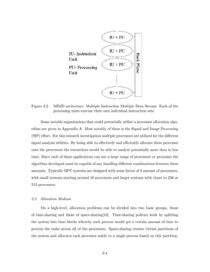
Figure 2.2 MIMD arcitecture: Multiple Instruction Multiple Data Stream. Each of theprocessing units execute their own individual instruction sets.
Some notable organizations that could potentially utilize a processor allocation algo-
rithm are given in Appendix A. Most notably of these is the Signal and Image Processing
(SIP) effort. For this research investigation multiple processors are utilized for the different
signal analysis utilities. By being able to effectively and efficiently allocate these processes
onto the processors the researchers would be able to analyze potentially more data in less
time. Since each of these applications can use a large range of processors or processes the
algorithm developed must be capable of any handling different combinations between these
amounts. Typically HPC systems are designed with some factor of 2 amount of processors,
with small systems starting around 16 processors and larger systems with closer to 256 or
512 processors.
2.2 Allocation Medium
On a high-level, allocation problems can be divided into two basic groups, those
of time-sharing and those of space-sharing[13]. Time-sharing policies work by splitting
the system into time blocks whereby each process would get a certain amount of time to
process the tasks across all of the processors. Space-sharing creates virtual partitions of
the system and allocates each processor solely to a single process based on this partition.
2-4
lU- Instruction Unit
PU- Processing Unit
lU + PU
lU + PU
lU + PU
n
P*
lU + PU

That process would then have total control of each of the processors in its partition. The
process however would be limited to only the processors within its partition.
An examination of the literature shows that a vast majority of the allocation studies
have been based on space-sharing approaches[13][68]. Time-sharing does have its advan-
tages, and thus should be examined, for as there is no free lunch for algorithms[84], their
can be no free lunch for every problem either. Thus no single solution can be used as the
most optimal choice for all problems.
Time-Sharing Approaches. Time-sharing approaches to processor allocation occurs
when the processing time is divided up such that each process has a set amount of time
to execute. Thus each process is given access to all of the processors they require, just in
discrete time increments. In general time-sharing approaches can be divided up into two
sub-groups: coordinated and uncoordinated[13].
Figure 2.3 Coordinated time-sharing processor allocation approach. Each process isgiven a time slice on the system such that all processors are available to eachprocess only during its time slice.
A coordinated time-sharing approach to a distributed system occurs where each
process is given a time-slice. During that time slice the process has full access to all of the
resources of the distributed system. Once the time slice has completed, all of the resources
then transfer to another process. This type of approach works best on systems with a
small granularity and centralized memory[13]. The small granularity is important so that
2-5
Processors
Process 2

the processes can execute fully in their limited time slices. Centralized memory allows
for a minimization of the overhead associated when the process is preempted. Figure 2.3
illustrates this process, at each time slice the processes switch such that for each time slice
each process can use all of the processors on the system.
When this is run on a system with distributed memory the transfer and storage
of data has a tendency of overwhelming any advantage that otherwise would be possible
from the policy[13]. To start with, the initial program data needs to be resident on every
machine a priori to execution. Then, during runtime the state of each of the processes
must be transmitted to each of the processors so that they can each continue working on
the program[13]. This transfer at each time frame generally makes this type of approach
excessively expensive for standard HPC systems.
Figure 2.4 Uncoordinated time-sharing processor allocation approach. Each process isallowed to use any processor at any time slice depending on the applicationneeds. Thus the process is allowed to roam across the network.
While the coordinated approach gives each process a single-time slice by which to
use every processor simultaneously, an uncoordinated time-sharing approach allows for the
processes to be executing during different time-slices. In this manner each of the processors
can work autonomously from the rest. Thus in this type of system one job can be running
at different times on different processors. The major disadvantage to this approach is
that the communication necessary to support each process being preempted at different
2-6
Processors

time slices requires excessive overhead by both the backplane and the underlying system
hardware. An example of this type of of approach is given in Figure 2.4.
Space-Sharing Approaches. There are many approaches that have been researched
for load balancing a distributed architecture based on a spatial partitioning policy. These
approaches can be nominally grouped into three basic classes: Static, Quasi-Dynamic (also
known as semi-static), and Dynamic[26, 13]. The concept behind dividing up the processor
domain is a result of the fact that many programs have an optimum number of processors
such that any additional processors does not improve the performance of the algorithm. In
many cases the additional processors does only add overhead to the overall execution[13].
In fact most programs have some cost optimal point where the addition of extra processors
is not advantageous to computation[71].
A static optimization creates an a priori solution of processor assignments that des-
ignates a partition of the processors prior to the system beginning its computations. This
allocation, once set does not change for the duration of the distributed system.
Quasi-dynamic load-balancing occurs when the state of the system changes discretely
and infrequently. Thus the optimization algorithm creates discrete solutions in parallel with
the other computations being executed on the system. These changes are only invoked to
the system at specific intervals during the system’s execution. It is the goal of this algorithm
that the infrequent changes would improve the overall runtime of the system.
Dynamic load-balancing occurs continuously during execution. The system must de-
cide as to whether any changes to the system would improve the efficiency or effectiveness
of the processes being executed. If a change is computed that would improve the perfor-
mance of the system it is implemented immediately. By enacting the changes in real-time
the algorithm can continuously improve upon the system.
Static Load Balancing Optimization. In a statically load balanced system the
processors are allocated a priori to any execution of the tasks intended to be executed.
Once these partitions are made they are fixed for the duration of the execution [13] [39].
Jobs are allocated to these partitions either by the user or by the system scheduler based
2-7

Figure 2.5 Static partitioning of a 16 processor system with 4 partitions. Each shadingrepresents a different allocation partition.
on the characteristics of the job. Figure 2.5 depicts one possible allocation strategy of a
sixteen processor system broken up into four different allocation regions.
Once the partitions have been created the processes are set to execute in their allo-
cated spaces. If a new process is to be inserted into the system then it is placed into what
is known as a system ready queue and waits till the next partition is available for it to use.
Thus each partition is assigned one and only one process, and the process has exclusive
rights to all the processors in that partition. Once the process has finished, the partition
is returned to a free partition pool for future assignment [13].
This system is effective for stable, long-term program executions, where there is not
a need for changes to the allocation space for each process. For most real world systems the
size of the programs being executed does change. These changes in program sizes create
an ineffective use of resources with static partitions. This disadvantage can be depicted
through the understanding that each partition can be used by only a single process. Thus if
a process uses less processors than a partition contains, those extra processors go to waste.
Conversely, if a task requires more processors than a partition allows, it must use more
than a single partition, again with the potential of wasting resources if the processors are
not fully utilized. For example, Figure 2.6 depicts a four processor partition, but with a
process that only requires two processors, the other two processes are not used. Figure 2.7
illustrates what happens when the processes require more processors than their partition
is allotted, also potentially leading to the poor utilization of resources.
2-8
Processors

Figure 2.6 Static resource underutilization. A four processor static partition using onlytwo processors being utilized results in a waste of resources for the distributedsystem, which is a major disadvantages of a static allocation. policy.
Quasi-Dynamic Optimization. A quasi-dynamic load balancing policy attempts
to overcome the mismatch between an allocated block size and a process’s needs that are
created through static approaches. This policy allocates the processors in a static fashion,
with the difference occurring in that the partitions can change during runtime for pro-
cesses that request a change in resources[13]. However, once the partition is created it is
not permitted to change until some specific event occurs such as [62]:
• Process Completion, where a process finishes execution and no longer needs it’s re-
sources. The processors that were assigned to this application can then be reassigned
to other processes.
• Process Arrival, where a new process enters the system for execution. This change
to the state of the system allows the newly arrived process to be immediately instan-
tiated onto the available processors.
• Allocation Change, where the processors are reallocated based upon some new infor-
mation about the state of the system. One example being if a process required a
change in processor amount during execution.
Studies have shown that this approach to processor allocation has results that are
practically identical to that of a static approach [13]. However, there does exist a grey
area, especially when examining reallocations that occur via system state information
changes. This class of events can be considered to provoke changes to the system that are
2-9

Figure 2.7 Static resource overflow. A process that uses more than a single partitionof processors for a twelve processor static partition system divided into twopartions of six processors each. The processors within the thick rectangle areused by the process; the other three processors are wasted resources.
more closely related to dynamic allocation strategies, which have been shown to be more
beneficial than that of the static methodology [13].
Dynamic Optimization. Whereas quasi-dynamic policies takes into account the
different sizes of executing programs at the beginning of their execution, it typically does
not take into account how the partition sizes might need to vary during execution. As
mentioned earlier, there is some grey area to this claim in that allocation changes based
on system state information can be viewed as the same type of changes that a dynamic
policy invokes. In order to handle these changing partition sizes during runtime dynamic
policies have been developed. Dynamic processor allocation policies continuously change
the processor allocations throughout runtime. Thus, if a process no longer needs a processor
during runtime, a dynamic policy would reallocate that processor so that it could be used
by a different process. Overall this ensures that the system resources are utilized to their
fullest.
One disadvantage to this method lies in the cost of deallocating a processor from one
job and reassigning it to another. As long as the cost of preemption remains small this
type of policy can be effective. For shared memory systems a low cost for reassignment is
2-10
Partition 1 ^^ Partition 2
n utilized Processors (^ Wasted Proces sors
typical. A distributed memory system typically would not have as low an overhead cost as
the entire process would have to be relocated each time a new allocation is performed[13].
2.3 Objective Via Symbolic Notation
Their exists a variety of objectives that can be examined for a load balancing sys-
tem. When incorporating the temporal aspect of a system for scheduling the processes
these objectives could include completion time (makespan), mean/maximum flow time,
mean/maximum tardiness, mean/maximum machine idle time, mean load and others [32].
When focusing only on the allocation portion of the system without regards for the fu-
ture executions a different set of objectives including processor load performance, intra-
processor communication costs should be examined[38]. With this in mind we focus our
discussion to those objectives that do not rely on temporal based allocation.
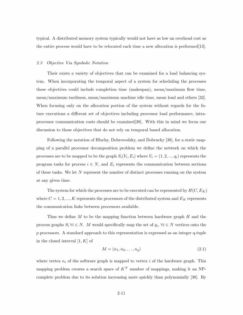
Following the notation of Hluchy, Dobrovodsky, and Dobrucky [38], for a static map-
ping of a parallel processor decomposition problem we define the network on which the
processes are to be mapped to be the graph Si(Vi, Ei) where Vi = (1, 2, ..., qi) represents the
program tasks for process i ∈ N , and Ei represents the communication between sections
of these tasks. We let N represent the number of distinct processes running on the system
at any given time.
The system for which the processes are to be executed can be represented byH(C,EK)
where C = 1, 2, ...,K represents the processors of the distributed system and EK represents
the communication links between processors available.
Thus we define M to be the mapping function between hardware graph H and the
process graphs Si ∀i ∈ N . M would specifically map the set of qi, ∀i ∈ N vertices onto the
p processors. A standard approach to this representation is expressed as an integer q-tuple
in the closed interval [1,K] of
M = (n1, n2, . . . , nq) (2.1)
where vertex ni of the software graph is mapped to vertex i of the hardware graph. This
mapping problem creates a search space of KN number of mappings, making it an NP-
complete problem due to its solution increasing more quickly than polynomially [38]. By
2-11

being classified as an NP complete problem this type of problem cannot be solved in
polynomial time, thus the time necessary for the algorithm to solve the problem increases
exponentially with the size of the problem.
In a single process(N = 1) static mapping problem the overall system would be
optimized such that at runtime the mapping M minimizes the completion time of the
single process. This is done by balancing the load across all of the processors as well as
minimizing the communication that needs to be done between processors.
For a single process system if we define the load of processor j to be Lj , then with
K processors the average load (L) can be defined as
L = 1/KK∑
j=1
Lj (2.2)
and thus the load imbalance (LIj) of any processor j would be
LIj = |Lj − L| (2.3)
and the overall cost of the imbalance (CLI) for the system would be
CLI =
K∑
j=1
LIj (2.4)
The communication cost (CCqr) of communication between tasks q and r can be
calculated as
CCqr = Cqr ∗ dM(q)M(r) (2.5)
where Cqr is the size of the message being sent, and dM(q)M(r) is the distance between the
nodes. Thus the overall communication cost (CAC) is
CAC =N∑
q,r=1
CCqr (2.6)
2-12

Another factor that needs to be considered when designing this type of system is the
link imbalance resulting from the backplane topology. If we let ADli be the amount of
data transferred across the link li then we could find ADli as
ADli =N∑
q,r=1
Cqr ∗RAM(q)M(p)(li) (2.7)
where RAM(q)M(p)(li) would be equal to 1 if the routing algorithm RA sent information
along link li and 0 otherwise. The mean amount of data (AD) then would be
AD = 1/TT∑
i=1
ADli (2.8)
and the imbalance (ADIli)would be
ADIli = |ADli − AD| (2.9)
Given all this information we can develop the cost function with coefficients β, α, γ.
CF (M, t) = βFvertex(M, t) + αFedge(M, t) + γFroute(M, t,RA) (2.10)
Where we define different potential functions for each part to be
Fvertex(M, t) = β(t)K∑
i=1
|Li − L| (2.11)
Fvertex(M, t) = β(t)K∑
i=1
(Li − L)2 (2.12)
Fvertex(M, t) = β(t)maxi(Li) (2.13)
for Fvertex and
Fedge(M, t) = α(t)∑
i,j=1
CCij (2.14)
2-13

Fedge(M, t) = α(t)maxij(CCij) (2.15)
Fedge(M, t) = α(t)∑
j=1
(CCij) (2.16)
for Fedge, and
Froute(M, t,RA) = γ(t)T∑
li=1
|ADij − AD| (2.17)
Froute(M, t,RA) = γ(t)T∑
li=1
(ADij − AD)2 (2.18)
Froute(M, t,RA) = γ(t)maxli(ADli) (2.19)
for Froute. These formulae are easily expanded to greater than one process by summing
each process’s objective value across all processes, thus for any generic static mapping of
K processors we would have
CF (M,K, t) =K∑
i=1
CF (M, t) (2.20)
It can then be seen that for any instance of time, this evaluation would measure the overall
effectiveness of an allocation strategy of the system. Thus even for a dynamic system this
equation is a measure of the effectiveness of a given allocation strategy at any particular
moment in time.
The edges, vertices, and routes that these formulae deal with are each indicative of
parts of the real-world problem that they are modelling. The edges correspond to the
communication links and the value for the edges relate directly to the communication
time that the communication link represents in a real world network. The vertices of the
graph represent the different processors of the system such that the value represented by
each Fvertex models the calculation load performance each processor is capable of. The
route thus is the overall communication cost between two processors given their relative
separation, this is primarily influenced by the backplane of the HPC system.
2-14

Thus, the overall objective for this basic allocation problem is to minimize the overall
cost or
minCF (M,K, t) (2.21)
As can be seen the overall objective for even a simple load balancing problem is not
one but multiple separate objectives, thus placing this problem in the multiobjective class
of problems (MOPs). These objectives are determined by their respective weights α, β, γ.
Dependent on the needs of the system the user can thus a priori adjust these three weights
in order to find some optimal stability of the system. Another option the decision maker
has is to a posteriori select a Pareto optimal solution. While these objectives are important
for a processor allocation problem, they are by no means the only objective functions that
can be examined for this type of problem. The engineer of the allocation strategy can
include any objective value deemed important based on the specific application that is
going to use the allocation policy.
By having multiple objectives available the algorithm designer has a couple of options
available for presenting the results. As explained in Appendix B, there are a variety of
approaches for dealing with multiple objectives. The decision of which approach is to be
used should be done prior to algorithm development as it does effect the algorithm choice.
2.4 Flexibility
The flexibility of a distributed system relates to the systems ability to allow for
process preemption. Once a process is given its partition, it may or may not be able to
move its processing to other processors. A process is said to move when, during runtime,
it either gives up some of its currently used processors, or adds new processors to those
already in use. Those processes that can move are called preemptive processes [71]. An
allocation policy must decide whether to handle preemptive processes or whether it should
simply assume all processes are non-preemptive. In order to accomplish this the advantages
and disadvantages of each approach should be examined.
A non-preemptive approach to processor allocation problems makes the assumption
that none of the processes can be preempted. This is the simpler of the two approaches,
2-15

allowing the programmer to simply ignore the preemptive ability of some processes. A
static spatial processor allocation policy takes this type of approach to partitioning the
system[13].
Figure 2.8 Process preemption capabilities example. Preemption policy for a six-processor three-process system. Processes 1 and 2 are both preemptible andtherefore can give up or use new processors during runtime. Process 3 isnot preemptible and therefore must remain on the processors it was assignedinitially.
A preemptive approach, on the other hand makes the assumption that some, but not
necessarily all processes can be preempted. Figure 2.8 illustrates this in that processes 1
and 2 are preemptible, but process 3 is not. Depending on the design of the algorithm
processes can be specified as to their ability to be preempted. Taking this into account and
allowing for preemption is how a dynamic allocation policy works. Without preemption
the processes would be unable to move from the partitions that they were initially started
from. Some of the pitfalls of the preemptive allocation policy is that preemption creates an
overhead that must be examined and measured so that the amount of preempted processes
is limited such that it does not adversely affect the overall system[62]. This measurement
must allow for the comparison of the cost of moving processes to the value gained by doing
such.
2.5 Arrival Process
The arrival process decision is based directly on the requirements of the parallel
structure that is being examined. Two common manners for which processes can arrive
2-16
Processors 3 4
Process 1 Process 2 Process 3

are batches or in a Poisson arrival stream. When processes arrive in batches there is a
large group of processes that are simultaneously executed onto the system. This does not
require that all processes must arrive at the same time, just that when they are ported
for execution that they are done so en mass as shown in Figure 2.9. One problem to this
type of approach is that while the processes arrive in groups, they may not be able to all
be processed concurrently based on the limitations of resources in the system.
Figure 2.9 Batch arrival process. Processes are executed on the system in large groupsat discrete time intervals.
A Poisson arrival process occurs when applications are begun one at a time in the
system. This would be the type of arrival process for a system where any given user could
input at any time an application to be executed on the system. An allocation algorithm for
this type of process would have to continually update and expand for continuous system
allocation so that any process could be inserted without any type of batching delay.
2.6 Service Demand Knowledge
The knowledge about the application service demand is based on what is known a
priori about how long it takes to service each process requested [62]. This type of knowledge
relates back to how the engineer intends to use the system. If it is known exactly what
type of applications are going to be executed, and how these applications are going to be
executed, then we can predict how much time the applications are going to take. This
type of knowledge is deemed a deterministic approach to scheduling. Conversely if it is
only known that the applications are going to be executed for some expected amount of
time, with some variance, then the arrivals fall under a probabilistic service demand model.
With either of these models the algorithm would require the expected service time, or the
service time distribution, of each application by which it could configure the allocation
algorithm, thereby leveraging this additional knowledge to the benefit of the system [39].
2-17
BATCH C Process 1 Process 2 Process 3
BATCH B Process 1 Process 2 Process 3
BATCH A Process 1 Process 2 Process 3

The final choice of device demand time would be where we have no knowledge about
what programs are going to use the algorithm. With this type of demand knowledge we
would simply have to include either user input or some other method for checking the
active processors to test for process completion.
2.7 Priority
When examining different processes for processor allocation it may be important to
have different priorities. With this type of system those processes with higher priority are
assigned to execute prior to those with lower priority. Thus the allocation of processors
is done such that the high priority processes receive the higher quantity of resources. If
there does not exist a need for such prioritization then all processes would be examined
as running equivalent priorities and would be given equal access to all processors on the
system.
2.8 Symbolic Problem Domain Description
Given these choices for the different alternatives of the processor allocation problem
domain we can begin to develop the overall symbolic problem domain description. Algo-
rithmically we assume we have some system with N processors that wants to execute some
K processes, K ≤ N . In the real-world problem we may have more then N processes,
yet only K of those are being assigned, and since we cannot assign more processes than
there are processors available, K must be less than N for the purposes of the assignment
problem.
The problem then is to map those K processes onto the N processors. The solution
that we are trying to find then is the set of all sets of processors allocated to each process.
Since we make the assumption that no two processes can use a processor simultaneously
we must create this mapping in a one-to-one fashion, thus preventing assignment of more
than one process to any given processor. The cost associated with each of the potential
mappings would be based on their objective evaluation as described in Section 2.3.
2-18
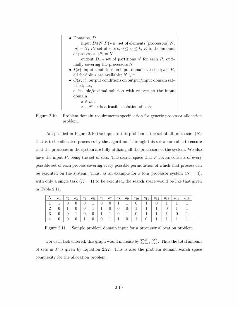
• Domains, Dinput Di(N,P ) - n: set of elements (processors) N ,
|n| = N ; P : set of sets s, 0 ≤ si ≤ k, K is the amountof processes, |P | = K
output Do - set of partitions n’ for each P , opti-mally covering the processors N
• I(x); input conditions on input domain satisfied; s ∈ P ,all feasible s are available; N ∈ n.
• O(x, z); output conditions on output/input domain sat-isfied; i.e.,a feasible/optimal solution with respect to the inputdomain
x ∈ Di;z ∈ N ′: z is a feasible solution of sets;
Figure 2.10 Problem domain requirements specification for generic processor allocationproblem.
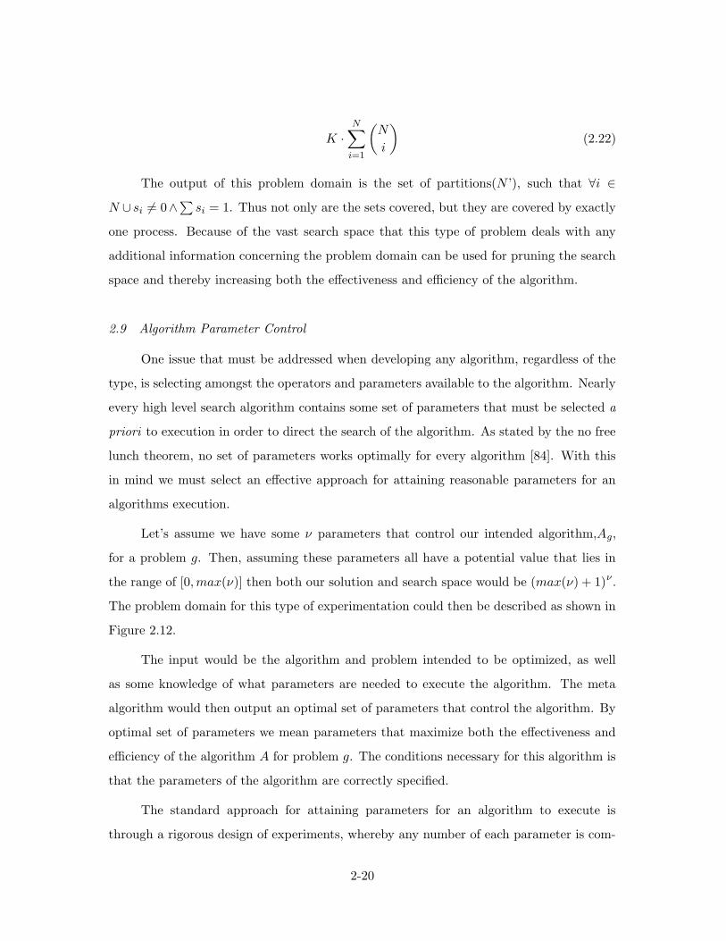
As specified in Figure 2.10 the input to this problem is the set of all processors (N)
that is to be allocated processes by the algorithm. Through this set we are able to ensure
that the processes in the system are fully utilizing all the processors of the system. We also
have the input P , being the set of sets. The search space that P covers consists of every
possible set of each process covering every possible permutation of which that process can
be executed on the system. Thus, as an example for a four processor system (N = 4),
with only a single task (K = 1) to be executed, the search space would be like that given
in Table 2.11.
N s1 s2 s3 s4 s5 s6 s7 s8 s9 s10 s11 s12 s13 s14 s151 1 0 0 0 1 0 0 1 1 0 1 0 1 1 12 0 1 0 0 1 1 0 0 0 1 1 1 0 1 13 0 0 1 0 0 1 1 0 1 0 1 1 1 0 14 0 0 0 1 0 0 1 1 0 1 0 1 1 1 1
Figure 2.11 Sample problem domain input for a processor allocation problem
For each task entered, this graph would increase by∑N
i=1
(
Ni
)
. Thus the total amount
of sets in P is given by Equation 2.22. This is also the problem domain search space
complexity for the allocation problem.
2-19
K ·N∑
i=1
(
N
i
)
(2.22)
The output of this problem domain is the set of partitions(N ’), such that ∀i ∈N ∪ si 6= 0∧∑ si = 1. Thus not only are the sets covered, but they are covered by exactly
one process. Because of the vast search space that this type of problem deals with any
additional information concerning the problem domain can be used for pruning the search
space and thereby increasing both the effectiveness and efficiency of the algorithm.
2.9 Algorithm Parameter Control
One issue that must be addressed when developing any algorithm, regardless of the
type, is selecting amongst the operators and parameters available to the algorithm. Nearly
every high level search algorithm contains some set of parameters that must be selected a
priori to execution in order to direct the search of the algorithm. As stated by the no free
lunch theorem, no set of parameters works optimally for every algorithm [84]. With this
in mind we must select an effective approach for attaining reasonable parameters for an
algorithms execution.
Let’s assume we have some ν parameters that control our intended algorithm,Ag,
for a problem g. Then, assuming these parameters all have a potential value that lies in
the range of [0,max(ν)] then both our solution and search space would be (max(ν) + 1)ν .
The problem domain for this type of experimentation could then be described as shown in
Figure 2.12.
The input would be the algorithm and problem intended to be optimized, as well
as some knowledge of what parameters are needed to execute the algorithm. The meta
algorithm would then output an optimal set of parameters that control the algorithm. By
optimal set of parameters we mean parameters that maximize both the effectiveness and
efficiency of the algorithm A for problem g. The conditions necessary for this algorithm is
that the parameters of the algorithm are correctly specified.
The standard approach for attaining parameters for an algorithm to execute is
through a rigorous design of experiments, whereby any number of each parameter is com-
2-20

• Domains, Dinput Di - the set of parameters ν , that control
the given algorithm Ag for some problem goutput Do - ν such that Ag(ν) executes optimally;
with regards to effectiveness and efficiency• Conditions:
I(x); input conditions on input domain satisfied;x ∈ ν
O(x, z); output conditions on output/input domainsatisfied; x, z ∈ ν, z feasible solution
Figure 2.12 Problem domain requirements for the meta algorithm
bined in such a manner as to search for effective parameters for the algorithm. This is
a very complex, and often extremely time consuming method as it requires examination
by the user of the results, tuning the future executions based on the results found by the
already completed executions. This is the tried and true method, used in most research
areas as the standard by which to conduct experiments. A different approach would be to
use a stochastic search technique in order to tune the parameters of a sub-level stochastic
search. In this manner the controlling operators of a search algorithm are determined via
some tuning execution of another search algorithm.
2.10 Summary
There are many choices that must be examined when building a processor allocation
system, including allocation medium, objective, flexibility, arrival process, service demand
knowledge, and priority. Each choice must be considered for applicability to a real world
system. A result is the symbolic load balancing problem domain developed in Section 2.8,
followed in Section 2.9 with a discussion on optimizing algorithm parameters. The next
chapter examines algorithms that can deal with NP-complete problems. Once an algorithm
is selected, the information from the background problem domain examination can be
applied to construct a real-world system.
2-21

III. Processor Allocation Algorithms
Many different methods have been implemented for solving domain allocation problems.
There are too many algorithms for a detailed description of each, but it is important to
examine a few approaches. This enables the selection of an effective algorithm for the
problem domain considered here. Due to the varied nature of the problem domain (see
Chapter II), the algorithms must be tuned to effectively map to user requirements. Thus
this chapter is as a sampling of algorithms for adapting to a specific problem domain.
While this is not an all inclusive list, the following are some of the algorithms used for
generating solutions to the allocation problem: Neural Networks [39], Linear Programming
[39], Opportunistic Load Balancing[39], Minimum Execution Time[39], Minimum Comple-
tion Time[39], Min-min[39], Max-min[39], Duplex[39], Simulated Annealing [39, 38, 26],
Tabu[39], A* [39], Orthogonal Recursive Bisection [26][65], Eigenvector Recursive Bisec-
tion [26], Recursive Spectral Bisection [65], Genetic Algorithms [78, 18, 39], Evolutionary
Strategies [30], Linkage Learning [7] , Diffusion Methods [38], Decision Directed Learning
[61], the Boillat Method [38], and Finite Automata [77]. These algorithms represent a
collection of both deterministic and stochastic search heuristics that have been used for
dealing with the processor allocation problem. Deterministic algorithms, by definition, uses
an incremental, repeatable approach for finding solutions[52]. Some of these algorithms use
problem domain knowledge in order to generate solutions, others use incremental search
heuristics to search the entire search space and choosing which solution is best for the sys-
tem. Stochastic algorithms, on the other hand, use random number generators to search
for solutions. Due to this randomness these algorithms can have differing solutions for each
execution of the algorithm. This makes the algorithms search a variety of locations the
search region without specifically enumerating each possible solution. This in turn allows
for solutions that are close to optimal but in a time frame that could be faster than their
optimal-search deterministic counterparts.
The algorithms examined in this chapter give a good overall picture of methods used
for load balancing optimizations, as well as potentially being implemented for a meta-
control algorithm. Three of these algorithms are deterministic in nature with only one
of which yielding a complete search of the search space to find optimal solutions. The
3-1

Algorithm Type Guarantee Optimal? Time
Neural Networks Deterministic no < NPLinear Programming Deterministic no < NP
Opportunistic Load Balancing Deterministic no < NPMinimum/Maximum Execution Time Deterministic no < NP
Min-Min, Max-Min, Duplex Deterministic no < NPSimulated Annealing Stochastic infinite time < NP
Tabu Deterministic no < NPA∗(Best-First Search) Deterministic no < NP
Orthogonal Recursive Bisection Deterministic no < NPEigenvector Recursive Bisection Deterministic no < NPRecursive Spectral Bisection Deterministic no < NP
Genetic Algorithms Stochastic infinite time < NPEvolutionary Strategies Stochastic infinite time < NP
Linkage Learning Stochastic infinite time < NPDiffusion Methods Deterministic no < NPBoillat Method Deterministic no < NP
Set Partitioning Algorithm Deterministic yes NP
Table 3.1 Load balancing algorithm descriptions
final two algorithms are stochastic in nature and use high level heuristics to effectively and
efficiently search the problem domain search space. Each of these algorithms are examined
with regards to their applicability to the allocation problem. Through this examination we
get an understanding of some of the different approaches and how feasible their solutions
are for use in the processor allocation problem.
The first algorithm we examine, in Section 3.1, is a classic set partitioning problem
(SPP) algorithm. This algorithm provides a guaranteed optimal solution as it searches the
entire search space for the problem. This algorithm is selected for analysis since it maps the
allocation problem into the classic Set Partitioning Problem and finds an optimal solution
using a well known algorithm. A simpler set of deterministic algorithms is explained in
Section 3.2 with a description of the max-min, min-min, and duplex algorithms. This
set of algorithms represent some of the more basic strategies for load balancing via a
greedy heuristic. These algorithms do not guarantee an optimal solution but they do
make a high-level search of the search space. The final deterministic algorithms that are
examined are the Orthogonal Recursive Bisection and the Eigenvector Recursive Bisection
algorithm in Section 3.3. These algorithms are problem domain specific heuristics that
3-2

have been developed as a more efficient method of finding solutions that are effective but
not necessarily optimal.
The final two algorithms that are examined in this chapter are the stochastic search
techniques of Simulated Annealing(Section 3.4) and Evolutionary Algorithms(Section 3.5).
In any finite time neither algorithm guarantees optimal solutions. However, both of these
stochastic techniques have been shown to find solutions that are closer to optimal than
the non-optimal discrete search techniques in a time frame that is much less than the
optimal discrete techniques[39]. These two algorithms are the fundamental algorithms for
stochastic search. They are based off of different real-world phenomena that are mapped
to the computational search space environment. Simulated annealing uses physical cooling
temperatures as a model, while evolutionary algorithms use biological evolution as its
model. These algorithms were both selected based on their historical effectiveness for
finding effective solutions to the allocation algorithm[39].
In each algorithm section the algorithms are presented in a pseudo-code notation as
developed by Lamont[45]. This format presents the input, output, and problem domains
as Di, Dp and Do respectfully. The algorithm itself is shown as a combination of six basic
operations: Next-state candidates, next-state generator, feasibility, selection, solution, and
objective. The next-state candidates presents the collection of all potential solutions.
The next-state generator selects from these next-state candidates those that are potential
solutions for the current phase of the algorithm. These potential solutions are filtered
through a feasibility operation that selects only those solutions that are within the feasible
region of the algorithm. Next the selection operator selects which members are to be
kept for progression to the next phase of the algorithm. The solution operator provides
some metric as to when the algorithm is finished, while the objective operator states what
the goal of the algorithm is. The combination of these components generates a complete
algorithm.
3.1 SPP Algorithm
The processor allocation problem can be mapped directly into a set partitioning
problem(SPP). The goal of the SPP is to find the minimal cost cover set that covers all
3-3

elements without overlap[15]. If we set all the cover sets so that they consist of all of
the different combinations of processors that each process can have, and we set the cost
of each set to some function of the overhead cost for running that set of processes, then
the solution to the SPP would be a minimal cost allocation of processes to processors, the
processor allocation problem. Since in our distributed system there cannot be an overlap
of processes on a single processor, a solution to the SCP would not suffice. Only with the
constraint that there is no overlap, ie the SPP, is the solution able to be feasible for a real
world processor allocation.
The generic processor allocation SPP algorithm domain can be explicitly written out
using the notation of [45] as illustrated by Figure 3.1. This solution uses an algorithm de-
veloped by Christofides for solving the SCP/SPP but with refinements so that it is directly
applicable to generic processor allocation problems. Set covering and set partitioning prob-
lems are classical NP-complete problems [52]. As can be seen by this direct mapping, even
a simple allocation of processors across a distributed system finds itself in the NP-complete
class of problems. By adding parameters for examination such as communication overhead
or processor capabilities, the complexity of the algorithm used for solving the processor
allocation must also increase, thus making the already NP-complete problem even more
difficult.
3.2 Max-min, min-min, duplex
Max-min, min-min, and duplex all work off of the same basic principle, they are
simple algorithms that move through the unassigned processes and assign them to the
processor that has the minimum expected completion time for that process. Let us use T
to represent the list of unassigned tasks, then at each step the set of minimum completion
times(ct) M for all processors P is found for each process t ∈ T .
M = min ct(t, p)∀t ∈ T, ∀p ∈ P (3.1)
Then, for min-min, the task with the overall minimum completion time from M is
assigned to the corresponding machine. Because this heuristic takes the minimum task it
3-4

• Domains, Dinput Di(N,P )N - set of elements (processors) n, |N | = nP - set of sets s |s| = n, 0 ≤ si ≤ k, where k is the amount of processesDp - partial set of covers N ′ of elements with ∀si ∈ P, si ∈ PEl - partial set of elements n ∈ N .L(ci) - list of El sets covered at cost ci.output Do - set of set-partitions N ′ of elements with ∀si ∈ N ′, si ∈ P
• ConditionsI(x); input conditions on input domain satisfied; s ∈ P , all feasible s are avail-
able; n ∈ N .O(x, z); output conditions on output/input domain satisfied; i.e.,
a feasible/optimal solution with respect to the input domainx ∈ Di;z ∈ N ′: z is a feasible solution of sets, F ′; F ′ ∈ Do;
• Operationsset of candidates (P ′) - reformat SPP table by block covers - tableau, find all
min-set-covers (Di) and put into Dp.
– Reduction Possibilities
if ∃ni ∈ N, ni * sj∀j ∈ P , then no solution exists
if ∃ni ∈ N, ni ∈ sk ∧ ni * sj∀j 6= k ∈ P then sk is in all solutionsnext-state-generator (N,P )- tableau (N,P ), explicit part of Di. P ′ := P ′ −
si∀si ∈ Dp
selection - select sj that covers uncovered ni at min cost in tableau, such thatprocess has not yet been chosen, sj * Dp. sj ∈ P ′
feasibility (P ′, n, s)- n ∈ N , sinP , ∀i ∈ N, si ∈ P ′∑
si = 1, P ′ ∈ Dp
if ni ∈ sj ∧ ni * Dp∀i ∈ Dp then Dp = sj ∪Dp
feasibility (sj ,L)- if E′ ∪ sj * El∀El ∈ L(ci), ∀c′ < ci ≤ c′ + c(sj) then reject sj .
solution (P ′,Dp,z) - ∀i ∈ N, si ∈ P ′ ∪ si 6= 0, P ′ ∈ Dp
objective - min(ci∀i ∈ P ′) = z = Dp
Figure 3.1 Algorithm domain requirements for the SPP algorithm(from Christofides[15])
3-5

has been shown to change the machine availability status by the least of any assignment
algorithm [39].
Max-min is different only in that instead of assigning the task with the minimum
completion time to the corresponding machine, max-min assigns the task with the overall
maximum completion time. By assigning tasks in this order, max-min attempts to alleviate
the penalties that occur from those tasks with longer execution times, and thus balancing
the overall system.
The duplex algorithm does both the min-min and the max-min and chooses for itself
the best value from the two.
• name: MinMin Algorithm• domains:
– Di is the set of all elements U to be assigned tothe graph G
– Dp is the set of minimum costs of elements of M ,and the current set of assigned elements S ′
– Do is the set S whose elements are mapped to Gbased on min cost
• operations, F: I(x); x ∈ Di O(x, S); x ∈ Di, S in Do
I ′(x,M, S′); x ∈ Di, M , S′ ∈ Dp;
– next-state candidates: set of all unassigned ele-ments U , with minimal completion costs generatedas M
M = min0≤j<µ(ct(ti,mj)), ∀ti ∈ U– next-state generator: U −→ U ∩ S ′
– feasibility: S′ is an incomplete spanning tree, S ′ ∈Dp
– selection: S ′ −→ S′ ∪min(ct(ti,mi))∀i ∈M– solution: U = ∅
– objective: min costS
Figure 3.2 Algorithm domain requirements Min-Min algorithm
The algorithm domain for the Min-Min problem is given in Figure 3.2. The only
difference between the min-min algorithm domain and the max-min algorithm domain is
that the max-min algorithm domain selects the maximum cost elements to be added to S
3-6

first. Thus it uses the same set M , just from this set it chooses the maximum element to
be added to the solution at each state.
3.3 Orthogonal Recursive Bisection
Orthogonal recursive bisection continuously cuts the graph in half, alternating be-
tween vertical and horizontal cuts. These cuts are typically made based on the physical
structure of the problem.
The principal behind this approach is that there is a natural parallelism and division
by using only half of the graph each time. By splitting each section of the graph in half and
alternating processes of each of the split halves the load is effectively distributed equally.
This is of course with the assumption that the load is homogenous throughout the problem
space [26].
This approach is done by finding some median for each graph section and then
grouping the graph nodes for that section in accordance to whether they are greater than
or lesser than that median. The orthogonal recursive bisection specifically alternates the
median between the different available axes so that the bisection occurs in different axial
directions each time through.
Eigenvector Recursive Bisection. Eigenvector recursive bisection cuts the graph in
half each time, these cuts are made based on the eigenvector of the matrix as opposed
to the mean used in the orthogonal recursive bisection approach. This approach tries to
mimic the results of a neural net. It is a more computationally expensive method than the
orthogonal recursive bisection heuristic, but has proven to be more effective as well [26].
The algorithm domain is the same as that given in Figure 3.3 with the exception that the
next-state generator splits the graph based on the eigenvector as opposed to the median.
3.4 Simulated Annealing
Simulated annealing is a method by which the system is made analagous to a slow
physical cooling temperature. This is one of the more common approaches to processor
allocation problems [39, 38, 26]. What happens is that the system is given a temperature
3-7

• name: Orthogonal Recursive Bisection Algorithms• domains:
– Di graph G with set of all elements to be mappedT
– Dp S′ is the set of all sets of nodes from G, ∪S ′i∀i ∈
S′ ⊂ G
– Do S the set of all subsets of G such that all Tcan be mapped to G, one T per subset of S
• operations, F: I(x); x ∈ Di O(x, S); x ∈ Di, S ∈ Do
I ′(x,M, S′); x ∈ Di, S′ ∈ Dp;
– next-state candidates: S
– next-state generator: S ′ −→ (12)Si∀i ∈ S– feasibility: S′ ∈ Dp
– selection: S −→ S
– solution: | S |=| T |– objective: min costS
Figure 3.3 Algorithm domain requirements Min-Min algorithm
T . The algorithm then iteratively proposes changes to the system, slowly decreasing the
temperature. This change is evaluated with the cost function based on the objective
chosen, we allow the cost function to be CF (M, t). Then, if the cost function decreases
from what it was at the previous state then the change is accepted unconditionally. If
the cost function increases from the previous state then the change is accepted with a
probability exp(−δCF (M, t)/T ), this is known as the Metropolis criterion[26, 38].
The concept behind simulated annealing is that it is necessary to use a change in
temperature δT that is small enough that the system can change between states of the
system, yet large enough that the solution doesn’t get stuck in a local optima. If the
temperature is too low then the system mimics a simple hill climbing algorithm and stops
at whatever local optimum it finds. If the temperature is too high then the algorithm acts
as a random search ignoring the cost function totally [1].
Thus the simulated annealing algorithm works by starting at a high temperature
that slowly decreases so that the solution analogously settles into the global optimum. In
3-8

fact, if this change in temperature is sufficiently slow enough, then the simulated annealing
algorithm guarantees that the global optimum is reached [31].
The basic approach to applying this heuristic to the load balancing problem is to
change a single node of the solution graph at random each time through the system. Then
determine whether to accept or reject based on the metropolis criterion, and continue on
until the temperature is near zero [26].
There are a variety of modifications available to this algorithm for tuning it to the
problem it is intended to optimize. The change in temperature δT can be modified to slow
or quicken the rate of convergence. The SA can be seeded a priori with good solutions
that it can build off of [39]. The original temperature T can be set to different values, as
can the stopping criteria. The different control procedures, solution modification, solution
comparison equation, and selection, can be modified as well for this algorithm[39]
Other than the generic modifications that can be implemented for the simulated
annealing algorithm, many specific adaptations of the simulated annealing algorithm have
also been suggested. One such addition is to allow multiple changes for each state. This
process is called collisional simulated annealing. Collisional simulated annealing allows
some fixed number of changes each generation, while at the same time checking for collisions
that adversely effect each other. The collision correction is done either by a rollback device
or by taking the possible changes, classifying them, and ensuring that all those changes
within each class do not collide. The rollback is highly expensive in terms of overhead
necessary to perform it. Research efforts have shown that collision classification tends to
fail to work when collisions occur between widely separated changes (in terms of Hamming
distance) [26].
The algorithm domain for the simulated annealing algorithm is given by Figure 3.4.
Where Φ represents the evaluation of the potential solution, m represents the mutation
operator that mutates the operator, δ is the cooling rate for temperature T , and Tmin is
the minimum temperature of the system.
3-9

• name: Simulated Annealing Algorithm• domains:
– Di is an initial random solution S ′, a system tem-perature T , and a cooling rate δ
– Dp is the set S′
– Do is the set S whose elements are mapped to Gbased on min cost
• operations, F: I(x); x ∈ Di O(x, S); x ∈ Di, S ∈ Do
I ′(x,M, S′); x ∈ Di, S′ ∈ Dp;
– next-state candidates: set of all available possibil-ities
– next-state generator: T → T−δT , S ′ −→ mΘm(S)
m a sequence m(i) of mutation operators
m(i) : X(i)m −→ τ
(
Ω(i)m , τ
(
Iµ(i), Iµ
′(i)))
– feasibility: S′ is an incomplete spanning tree, S ′ ∈Dp
– selection: S −→ S ′ when Φ(S′) < Φ(S) iff
rand[0, 1) > 1
1+e(Φ(S)−Φ(S′)
T)
– solution: δT < Tmin
– objective: min costS
Figure 3.4 Algorithm domain requirements for the simulated annealing algorithm
3.5 Evolutionary Algorithms
Evolutionary algorithms (EA) consist of a class of algorithms that use the concepts
of genetics to help enable them to explore the search landscape. EA’s have been used for
a wide variety of applications including processor allocation problems [30] [18] [7]. In an
evolutionary algorithm a collection of individuals each known as chromosomes, consist in a
group defined as a population. The population moves through generations by using genetic
operators such as mutation and recombination. Mutation works by inserting new genetic
material into the population, recombination by transferring preexisting genetic material
between two or more individuals of the population. There are many different varieties of
genetic operators each with different parameters that can be modified.
Random changes of the population via genetic operators is not enough to lead the
population to optimal solutions. Evolutionary algorithms must also use a type of selection
3-10

operator that identifies members of the population for propagation to the next generation.
These operators effectually lead the population to search in areas of higher fitness, thus
are able to obtain closer and closer to optimal results. Because selection operators use
stochastic control parameters EA’s are able to not confine themselves to one part of the
search area, and can thus search the entire landscape even while moving towards near
optimal solutions. For a more formal description of evolutionary algorithms, see Appendix
C. A pseudocode algorithm for a generic EA is given in Figure 3.5.
As explained by Merkle [48][47] this definition has advantages over Back and Schwefel
(see Appendix C) in that it is not limited to only a single operator for mutation, recom-
bination, nor selection, nor a single parameter for any operator. This algorithm definition
also allows for population sizes of µ′ + µ and µ′, which are indicative of µ + λ and µ, λ
algorithms. When λ = 1 the description can then also represents the µ+1 algorithm. The
final difference between Merkle and Back’s algorithms is that Merkle represents the fitness
evaluation as being a parameter of the selection operator as opposed to Back’s explicit
evaluation call.
t := 0;initialize P (0) := ~a1(0), . . . ,~aµ(0) ∈ Iµevaluate P (0) := Φ(~a1(0)), . . . ,Φ(~aµ(0))while (ι(P (0), /dots, P (t)) 6= true) do
· recombine : ~P ′(t) := r(t)
Θ(t)r
(P (t));
· mutate : P ′′(t) := m(t)
Θ(t)m
(P ′(t));
· select : ifχ
· thenP (t+ 1) := s(t)
(θ(t)s ,Φ)
((P )′′(t));
· else P (t+ 1) := s(t)
(θ(t)s ,Φ)
((P )′′(t) ∪ P (t));· fi· t := t+ 1;od
Figure 3.5 Merkle’s generic EA notation
Using 3.5 an evolutionary algorithm is defined such that
• I is a non-empty set,
• u(i)i∈N a sequence in Z+ (the parent population),
3-11

• u′(i)i∈N a sequence in Z+ (the offspring population),
• Φ : I −→ < a fitness function,
• ι : ∪∞i=1(Iµ)i −→ true, false(the termination criterion),
• χintrue, false,
• r a sequence r(i) of recombination operators r(i) : X(i)r −→ τ
(
Ω(i)r , τ
(
Iµ(i), Iµ
′(i)))
• m a sequence m(i) of mutation operators m(i) : X(i)m −→ τ
(
Ω(i)m , τ
(
Iµ(i), Iµ
′(i)))
• s a sequence s(i) of selection operatorsm(i) : X(i)s xτ(I,R) −→ τ
(
Ω(i)s , τ
((
Iµ′(i)+χµ(i)
)
, Iµ′(i+1)))
• Θ(i)r ∈ X(i)
r (the recombination parameters),
• Θ(i)m ∈ X(i)
m (the mutation parameters),
• θ(i)s ∈ X(i)s (the selection parameters),
The algorithmic complexity of an EA is equal to the amount of evaluations that
must be performed by the algorithm. Thus if we set tmax as the maximum amount of
evaluations that the algorithm must perform the algorithm would have a complexity of
O(tmax). As long as this number is relatively low this algorithm is efficient. As the amount
of evaluations increase the effectiveness in turn increases, but the efficiency decreases. The
only good thing is that the efficiency decreases linearly. Thus even with a large amount of
evaluations we still have an algorithm that is relatively faster than some of the deterministic
approaches.
3.6 Summary
As shown in Table 3.1, there are a large variety of algorithms available for allocating
processors. The six algorithms examined in this chapter, i.e., Set Partitioning, Max-
min/Min-min, Orthogonal Recursive Bisection, Eigenvector Recursive Bisection, Simulated
Annealing, and Evolutionary Algorithms, illustrate the types of algorithms available. The
selection of any algorithm depends on the choices made when developing the problem
domain. Each algorithm can produce a solution which is more applicable or more effective
based on the requirements of the system to be balanced. An understanding of how the
3-12

algorithms work is needed for effective mapping of the problem domain to the algorithm
domain and for producing solutions that meet application requirements.
The next step in model development maps the algorithm domain information to the
problem domain that best meets the needs of the intended system. This step entails se-
lecting an algorithm capable of addressing the problem domain with reasonable optimality
in a time frame acceptable to the user.
3-13

IV. High Level Design
From the previous chapters have explained the problem and algorithm domains. The first
step in their mapping is to examine the problem domain and select the development path as
indicated in Section 4.1. Next the actual modelling of the problem domain to the algorithm
domain mapping is accomplished (Section 4.2). Finally, the selection of an evolutionary
algorithm is given in Section 4.3.
4.1 Problem Depiction
Different available options as described in Chapter II are examined, specifically choos-
ing between the choices as listed in Table 2.1 which is again provided in Table 4.1 though
with the load balancing choices emphasized.
Allocation Medium:spatial vs. temporal
Objective:min communication vs. min processing vs. min routing
aggregate objective vs. Pareto multiobjective
Flexibility:non-preemptive scheduling vs. preemptive scheduling
Arrival Process:batch of applications vs. Poisson arrival stream
Service Demand Knowledge:none vs. probabilistic vs. deterministic
Priority:equal priorities vs. distinct priorities
Table 4.1 Decision choices for an allocation algorithm. The selected choices are itali-cized.
Allocation Medium. When choosing between a temporal or a spatial method for
processor allocation an examination of the literature confirm that a spatial approach is
the more common [13, 38, 18, 7]. For our purposes a spatial approach has the benefits of
4-1

allowing for a physical distribution of the processors. Since it is unknown what processes
are going to be executed on the processors we cannot determine a priori how much each
time slice each process requires for a temporal division. Also, since some of the programs
inevitably require a certain amount of processes to execute simultaneously across multiple
processors it is more effective to organize these processors such that their relative proximity
limits their communication overhead then to try to keep track of which processor each
task is located on and communicate across unknown amounts of network. One argument
against using a spatial based policy on a potentially heterogenous system is that the slower
processors can delay the overall computation. This problem can be surmounted by giving
these slower nodes smaller portions of the processes, or by defining the process blocks such
that the processors for each task are relatively equivalent.
Thus, the spatial partitioning policy is the more prudent method. It gives us the
advantage of proximity, which is important for a system that we have no a priori knowledge
concerning how much intra-processor communication the processors require. By using
this method the user also gains more control over what processes are assigned to what
processors, thus we can ensure that the overall system is loaded appropriately with respect
to the performance of each processor on the system. Also, since the system that this
research effort focuses on has such a high amount of unknowns with regards to the processes
being executed, we cannot guarantee that all of these processes would be able to support
the interrupts of the temporal based load balancing.
Spatial Policy Selection. We propose a system that works using a dynamic approach
to load balancing. By dynamic we mean that the system can, during runtime, change
the allocation space of processes so as to improve the performance of the system through
balancing the overall configuration as much as possible. Multiple studies have shown that
dynamic approaches have through multiple studies shown themselves to be more effective
than either static or semi-static approaches[13, 39].
The static policy has the advantage of being easy to implement as well as being
a very stable execution approach [13]. Unfortunately this policy does not allow for any
adaptation to changes in the system. It only allows for a specific amount of processes
4-2
to execute at any given time. If the amount of processes is greater than the amount of
partitions then those extra processes are not able to take advantage of the extra resources
that might be available on the system and thus are unable to be processed. On the other
hand, if the process requires more processors than its partition has then it would need to
take an additional partition in order to execute. These partitions may or may not be local
to one another depending on what else is running on the system. Again, any processors
that are not utilized by this process within these partitions would be wasted to the overall
system. This leads to a poor overall resource utilization within static partition policies[13].
In a dynamic policy the partitions change throughout runtime based on the needs
of the processes. One potential disadvantage to this approach is that if a process releases
one of its processors, which is then reassigned by the dynamic policy to a different process.
Then if the original process requires another processor, it is forced to use a processor that is
potentially distant creating an excessive amount of communication delays, or the algorithm
would force one of the more local processes to move so that the original process can claim
one of their processors. Either way this type of occurrence would be very expensive for
the processes involved. But, on the other hand, by allowing for dynamic preemption the
processes can be mapped so as to avoid routes with excessive communication as well as
allocating processors that are released by processes during runtime.
As with real-time scheduling systems, dynamic load balancing systems have often
been examined in an overly simplistic fashion due to academic constraints [46]. For this
reason this research investigation focuses on one part of the overall problem for scheduling
and allocating processes and processors in a real-time manner. While it is infeasible to
assume that this system perfectly mimics a real-world system we can limit our assumptions
concerning the different aspects of the system so as to minimize the amount of error that
occurs overall.
Objective. The objectives that need to be examined are all based on the overall
balanced allocation of the processors to the processes. The first objective that must be
examined is that the system does not use more processors than are requested for our
specific processes, but that it uses at least the amount of processors that are required
4-3

for each task. The reason that the lower bound exists is obvious. For the upper bound,
the amount requested, we do not want to waste processors on processes that cannot take
advantage of the resources.
Since preemption is a real-world item that can happen to a distributed process with
high cost, and potentially high benefit, we must take that into account for this system. A
balance must be made between the preemption that occurs because a task looses one of its
processors and the preemption that occurs when a task is given another processor for which
to use. Both cases need to be considered for both their advantages and disadvantages to
the system. If a processor is removed from a process, then that process must reallocate
its resources and redistribute itself, creating a large cost to the process and its overall
execution time. When a process is given a processor the process must also redistribute
itself to the new processor, this causes some overhead, but the hope is that the addition of
a new process is able to benefit the processes, and thus the system’s, overall performance.
Another objective that must be taken into account is the distribution balance. As
described in Section 2.3 if the processes run on a heterogeneous system then a skewed
distribution of processors could have an ill-effect on the algorithms performance [7]. Thus
it is important that the algorithm try to assign processors that are relatively comparable in
performance. Using this type of balancing the potentially heterogenous system is virtually
converted to as much of a homogenous system as possible. This allows those applications
being run to be able to make the assumption that they are running on a homogenous
system.
As with the processor balance of the system, the cost of communication must also be
examined. The algorithm must ensure that the overall communication overhead for each
process is minimized. To do this we have to consider the relative backplane speed as well
as the communication topology of the network with respect to the communication costs
between the different nodes.
The final objective that must be examined with this algorithm is the amount of
processes that are not executed. We clearly want to minimize the number of processes
that are not placed in the schedule, thus trying to run as many of the applications as
4-4

possible within the bounds of the constraints given by the amount of processors required
and requested for each process.
Flexibility. Not all processes are able to be preempted. Because of this the allocation
algorithm must take into account those algorithms that cannot be preempted. This is done
with a constraint on the algorithm such that those processes that are not preemptible
are not moved from their allocated processors in the next state of the system. Those
processes that are preemptible should be allowed to roam amongst processors, but the
evaluation function must take into account the high cost associated with preempting a
process. Whether or not a process is preemptible should be stated by the user of the
algorithm a priori to the execution of the algorithm so that the generated allocation
policy can ensure feasible execution of the tasks.
Arrival Process. The arrival process expected for this algorithm is a batch of pro-
cesses arriving in a Poisson manner. The batch of processes are entered by the user of the
algorithm for execution, once the batch is selected for execution the algorithm computes
the next state of the system and outputs that next state. This is not a static policy in
that the processes can arrive at any time either from the user of the system, or from the
underlying control program of the operating system itself. If either of these two control
components signal that a change to the system is necessary, the algorithm takes the current
state information and generates the next state of the system.
Service Demand Knowledge. There is no expected service demand of this algorithm.
It takes the information provided to it from the outside world and calculates the next
state of system whenever a change occurs. This change could be a process being finished
internally to the system, or some change based upon the needs of the user of the system.
Only at these points does the program recalculate the next state of the system. The ”time-
to-live” of the processes is not known either, thus the algorithm must be reactive instead
of proactive in its computations.
4-5

Priority. It is assumed that all processes entered into this system have equal priority.
No process is allowed to preempt another process based on the process priority, unless done
manually by the user of the system.
4.2 Representation
As with any algorithm the representation used is highly important to the develop-
ment. For the purposes of this research investigation the representation of the distributed
system’s hardware, and also the state of the system (as seen by the algorithm) are critical.
The key aspect of these representations is that they allow us to map the hardware metrics,
processor allocation, and the user execution requests all to a form that would be amenable
for algorithmic manipulation. The representations chosen must also be compatible with
the system model that is developed. Only through this compatibility can the algorithm be
mapped effectively to the problem.
Hardware. For representing the hardware it is not essential for us to have the absolute
values of the different processor speeds and communication latencies. It is important
however that some type of relativistic measurement exists so that we can compare how
each component works against the overall system. By taking a percentage approach to
hardware we allow ourselves to compare only how each part of the distributed system
works in comparison to each other without worrying about the real-world equivalent of the
performance metrics.
Since the system is assumed to be composed of a heterogenous set of processors, in
order to get the most performance out of the system, we need to be able to take into account
the different processors relative performances. Given that we have N processors we create
an array P of 1 . . . N such that P (i), 1 ≤ i ≤ N represents the relative performance of the
processor identified by i. The relative performance is defined as the percentage processing
capability against the optimal processor, or
P (i) =Pf(i)
max(Pf(j)∀j ∈ N)(4.1)
4-6

where Pf(i) is the performance of the processor i based on the metric decided upon
by the operator of the distributed system. Various metrics can be used based on the
desired accuracy desired by the administrator of the system. There also exists a variety of
benchmarks in the commercial world that can be used in order to measure the processor
capabilities.
The same type of measurement is to be done with the communication latencies of the
system. This time a matrix C is used such that Cij represents the relative communication
latency of processor i to processor j. Not all processors need to communicate, those that
don’t are represented by a 0 in the matrix showing that there is no direct communication
between the processors. By having the relative communication latencies between the dif-
ferent processors we can try to organize the processes so that the communication necessary
for the system is minimized.
One improvement that can be done to the system is to have the center diagonal of
the communication matrix be set to the processor performance results. In other words
Cii = P (i), ∀i = 1 . . . N (4.2)
This would minimally reduce overhead for the system and allow all the hardware informa-
tion to remain in a single matrix.
States. Time for the distributed system does not necessarily have to be based on a
standard clock. Instead a more practical manner for representing the transition of states
is that of being between states[71]. A state(S) is defined as the mapping of the processes
to the processor at some time of the system t. At any given time we define the system as
being able to support up to K tasks, K ≤ N . The effective and efficient mapping of these
tasks to the N processors is the overall goal of this system. A state at any given time S(t)
then consists of the following items:
Number of Processors (N) being the number of processors that the system has control
over for the current time step.
4-7
Number of Processes (K) being the number of distinct processes, or programs, that
the system is supposed to map to the N processors.
Current Reference List (Ref) being the identifying list of items that are in the
system. This list contains the information concerning each process that the system is
dealing with including the inputted identifier of the system, its numerical identifier in the
process assignment array, the preemption capability of each process and the number of
processors the user requested and required for the process.
Processor/Process Assignment Array (pAssign) being the array that assigns the pro-
cess given by it’s numerical process identifier (as stated in Ref) to the processor identified
by the index of the array, mathematically pAssign(i) = j where i is the processor number
(1 ≤ i ≤ N) and j is the process identifier (1 ≤ j ≤ K).
Since everything except pAssign is known a priori to the state it is the finding of the
near-optimal pAssign matrix that this is the focus of this research effort.
Requests. In order to go between states a request system is given that would represent
what changes to the current system need to be done in order to transition to the next state.
A request is defined with the following components:
Name being the unique identifier given to the process by the user.
Number Processors Required being the amount of processors the process requires for
execution.
Number Processors Requested being the amount of processors the user would ideally
like to have assigned to the process.
Preemptability being whether the process can be preempted.
Each request(rl), where l is the request identifier out of L total requests made, can
then individually impose upon the current state some change that would alter it when cre-
ating the next state. The collection of all of these different requests (R = r1, r2, r3, . . . , rL)
is the maximum differences between the current state (S(t)) and the next state (S(t+1)).
4-8

State Transitioning. Given that the system is at a current state S(t) with a list of
requests imposed upon it R(t) consisting of individual requests r1(t), r2(t), . . . rL(t). The
transition occurs when moving to state St+1 such that each of the requests has been im-
plemented on St to the maximum extent allowable given the amount of resources available
on the system. Specifically the reference list(Ref) and number of processes of state S(t) is
updated to include the new processes that have been added to the system, and remove all
the processes that have been requested to be removed from the system. Figure 4.1 depicts
a typical request list used to transition between states.
Figure 4.1 A standard request list used for providing information about the current stateso that the algorithm can effectively transition to the next state.
Once the reference list and the number of processes of S(t) is updated the new state
S(t + 1) is created with the initial assignment array being set to pAssign(t) minus the
processes that are removed.
At this point the new state is sent for processing by the algorithm for attempting to
find optimal processor assignment for load balancing. The only thing that is changed by
the algorithm is the assignment array (pAssign).
4.3 Evolutionary Generation
Given a representation of the state of the system, along with the method by which
the requests for changes to the system state are made an algorithm needs to be developed
4-9
Request List InformatJon pAssign[S(t)]^ ]] 11222233334444
K=£>4 1 1 16 0
Ref =-. lll^ \ Requests 14 2 16 01
ID =ij>4 2 16 Ot3=Preemptible ^ ^ 0:False, l:True
Processors Processors Required Requested

that can generate an optimized next state of the system. Due to the complex nature of
the search space[38, 65] an Evolutionary Algorithm (EA) is used . EAs have continually
shown their effectiveness for dealing with NP-complete problems[5, 75]. For the processor
allocation problem specific, EAs have been statistically shown to be more effective than a
range of other heuristic algorithms[39]. In fact we use three evolutionary algorithms for
this research effort. We have a primary EA, the allocation EA, that actually finds the
next state of the distributed system. In order to help evolve this EA, a meta-EA is used
for tuning the parameters of the allocation EA. The third EA is a competitive EA that
generates test strings to try to emulate and/or stump the allocation EA. The combination
of these second two algorithms helps to ensure that the allocation EA is an efficient and
effective heuristic.
As given by Michalewicz and Fogel, for every algorithmic design we must have at
least the following three items[52]:
• Representation
• Objective
• Evaluation
Thus for each of the EAs used we describe the problem they are designed to handle along
with these respective design items. This allows us to progress to the more detailed design
and actual algorithm implementation.
Allocation EA. The allocation EA is the primary heuristic for this research investi-
gation. It’s purpose is to actively divide the processors amongst the different processes.
Specifically this algorithm would make changes to the partitions such that the system
moves from a current state of the system, s(t), to a new state s(t + 1) while minimizing
the overall cost on the system and yet maximizing the effectiveness of the distribution of
processors. The representation used for this EA is based directly on the state information
described in 4.2. This allows for easy conversion via a graphical user interface between
the user and the allocation EA.
4-10
Because of all the variables in the system, the allocation EA must manage a com-
bination of objectives effectively. It must ensure that the processes have an appropriate
amount of processors based on the amount they respectively require/request. The prox-
imity of the different processors must also be examined. Each process that has more than
one processor must be organized such that the communication overhead between proces-
sors is minimized. Since the systems that this utility can be run on does not necessarily
require homogenous processors, nor homogenous communication links, these variables are
inputted into the algorithm in a representation such as described in Section 4.2 in order
for the EA to better balance the overall system.
The reason why this system would not be classified under a static configuration
resides in the fact that this system is able to update temporally. In a static environment
the system is constrained from the beginning to having partitions of certain dimensions.
If a program runs under these dimensions then the unused processors are wasted. If a
program requires more processors than a partition has available then it must use other
partitions, again wasting whatever processors are in its partitions that it does not need.
This proposed system tries to alleviate this problem by allowing the system to reallocate its
partitions as necessary. Thus a user at any time can execute processes on the distributed
system and the allocation EA would change the allocation space so that processors are
utilized to their fullest.
The evaluation function of this EA is based on minimizing the overhead cost objec-
tives and maximizing the hardware usage (with respect to the processes) at each change
in the systems allocation configuration.
Since this is to be developed into a utility that could be used by researchers visual-
ization of the system is important. A graphical user interface (GUI) for this algorithm is
incorporated so that commands for execution can be entered into the system. The GUI
allows the user to input requests for changes that are to occur for the next state of the
system. As shown in Figure 4.2, the GUI is a central point for examination of the critical
points of the algorithm including:
• Current State of the Distributed System
4-11

Figure 4.2 A visualization utility to display the information pertinent to the load bal-ancing algorithm. Included in this visualization is the communication costs,the current state of the system and the next state of the system. The userwould control the inputs to the algorithm via the GUI panel.
• Proposed Next State for the Distributed System
• Changes that are to occur to the Distributed System
Competitive EA. Though the allocation EA is designed for being able to be converted
so that it runs on a real-world distributed system, it is not used for beyond development,
testing and evaluation. Thus a simulation of potential inputs for the EA is necessary. That
is where the competitive EA comes in. The competitive EA is a coevolutionary algorithm
that uses the principle of competition for EA improvement as described in Appendix D.
It takes as input the state of the system as given by the allocation EA and produces, as
output, a new list of requests for the allocation EA to execute. In this manner it mimics
a user of the allocation EA system, specifically one who tries to stump the allocation
algorithm. The representation used for storing all of this information is identical to the
request list as described in Section 4.2 so that it can be easily imported into the allocation
4-12
1 1 M
^
j -— IL -I^T I - n
-- _ _ . _- __ _ _ , _ ^ _ _ um . 1. 1'
—1 - f - — -- - -1 - i:iiimrnktrm\
!
' l^-ll 1 1 ••'_a 1 1 1 _ _ _ _ _ 1 _ _, -^ 1
-—' — - - — — - - - ^ —- :a — i-mrrn^^pjttt*
— - - — — — - :- —f
- — ^M "Z'' tj'.*(
L ~ - - --' - -1 — VMM
1 14
1 1 1 H—H[>MI 1 11 1 jii b_ 1
II
EA, and also because it can better mimic the real world requests given to the allocation
EA.
The competitive part of this EA comes into play in that the development of new
request lists is based on the objective of making the allocation EA create bad partition
policies. Thus this EA helps us to discover sources that can be improved upon in the
allocation EA, as well as discerning problems that could occur based on the requests
possible from the user. The overall objective of the competitive EA is then to maximize
the evaluation of the allocation EA.
Meta- EA. The effectiveness of an EA can be largely based on the operators and
parameters chosen for implementation [5]. The analysis of parameters is a large com-
binatoric problem in itself [80]. Thus in order to further optimize the allocation EA a
meta-EA is developed that tunes the parameters. This meta-EA is used only on the initial
tuning of the allocation EA, and not for the actual running of the allocation EA itself.
The meta-EA is a separate EA that interfaces with the allocation EA and appropriately
tunes the parameters. Its objective is based directly on how effectively and efficiently the
allocation EA can handle requests given to it by the competitive EA. The representation
of the chromosomes within this EA are the different operators and parameters available
to the EA that it is tuning. It’s objective is to maximize the effectiveness and efficiency of
the algorithm that it is tuning. The meta-EA uses an evaluation function based directly
on the evaluation of the EA it is attached to for measuring effectiveness. For the efficiency
measure the evaluation is calculated based on the number of evaluations the sublevel EA
performs.
Since the meta-EA has two objectives to evaluate, those of effectiveness and of ef-
ficiency, a Pareto front analysis is employed. With this approach we can evaluate the
tradeoff ourselves as to what what of the two objectives is the more important a posteriori
to the execution of the algorithm.
4-13

4.4 Summary
The design discussed here begins to achieve the goals and objectives. The first
goal is achieved with choices as indicated in Section 4.1. The second goal is met by the
development of the allocation algorithm system in Sections 4.1 and 4.3. The third goal is
addressed by the algorithmic comparisons of the intended allocation EA system with other
available algorithms. The latter two goals are also addressed by the two coevolutionary
algorithms discussed in Section 4.3.
Both coevolutionary algorithms tune and adapt the allocation EA so that it is as ef-
fective as possible when introduced to a real world environment. The representation of the
system hardware allows for easy conversion from the development and testing arena to an
actual working system, allowing flexibility in the EA for evolving solutions. Through train-
ing on the competitive EA and tuning with the meta-EA, the allocation EA is developed
as robust software. However, the actual choices for EAs and operators to be implemented
are crucial to successful development. The incorporation of these details into the overall
algorithm is the subject of the next chapter.
4-14

V. Low Level Design and Algorithm Implementation
The primary focus of this research investigation is in the design and development of an
effective and efficient allocation EA. Two other coevolutionary EAs are interfaced to the
allocation EA to aid in its evolution and development. This chapter details the design of
each of these three algorithms. Also discussed are the different EAs: the allocation EA
(Section 5.2), the competitive coevolutionary EA (Section 5.3), and the meta-EA (Sec-
tion 5.4). Each of these discussions continues the initial design presented in Section 4.3.
An explanation on how each algorithm contributes is given in Section 5.5, and an imple-
mentation description given in Section 5.5.
5.1 GENOCOP III
The algorithm that is implemented for the different EA’s is a highly modified version
of Michaelewicz’s GENOCOP III program [50]. GENOCOP stands for GEnetic algorithm
for Numerical Optimization for COnstrained Problems[51]. It is a real-value genetic al-
gorithm that has proven itself successful at finding near optimal solutions in a variety
of problem domains [76]. The original idea behind the first version of GENOCOP was
to have a general and problem independent genetic algorithm that could handle different
constraints. This algorithm has since been expanded to GENOCOP III.
GENOCOP III took the ideas of it’s predecessors and incorporated an additional
population that allows it to search outside of the feasible region for near optimal points.
Thus it has two populations Psearch and Preference. The search population Psearch consists
of all points that satisfy the linear constraints of the problem. This population is identical
to the population of the original GENOCOP version. The second population, Preference,
contains only those points, taken from the search population, that satisfy all constraints
(linear and non-linear). Also, for ensuring that the search population does not stray too
far from the feasible areas a repair function is implemented that evaluates the search
population member based on some point chosen by the linear intersection between the
search member and a random reference member. With some probability the search member
then moves towards the feasible region. In this manner the GENOCOP III system can
5-1
search feasible and nonfeasible areas alike, but constrains the possible solutions as being
those points that are fully feasible.
The results found by using GENOCOP III have validated its effectiveness for a variety
of single objective experiments [76, 50, 51]. For our uses GENOCOP III has been modified
in a number of different ways. First, functionality is introduced for dealing with Pareto
optimization for multiobjective optimizations. It is also modified so that it has the capacity
for self procreation, whereby it could call itself for meta-evolutionary optimizations. In
this way the algorithm is able to improve the sublevel execution’s parameters to some
respectable level.
We also implemented a parallelization of the algorithm. An island model approach
is selected whereby multiple demes of both reference and search populations are executed
in parallel. Communication between the demes occurs with feasible members with the
best evaluation of the population transferred amongst the neighboring populations. This
transfer of individual solutions promotes the diversity of the different demes.
GENOCOP III pseudocode. Expanding on Merkle’s algorithm for evolutionary al-
gorithms, as given in Section 3.5 we can describe the generic GENOCOP III system in
Figure 5.1. This algorithm makes some modifications to Merkle’s original notation based
on it’s inability to define the specifics of the GENOCOP III system. First off, as Merkle
noted, neither his nor Back’s definitions take into account algorithms which terminate
based on a predefined amount of evaluations being reached. Second, because of the man-
ner that the GENOCOP III system is designed, we need to introduce the search population
with feasibility operators that are employed.
In this algorithm, other than explicitly declaring the different operators for the ref-
erence and search populations, the only real modifications made are that we have added
tmax to represent the maximum number of evaluations to be performed and tref represents
the amount of evaluations to evolve the search population prior to optimizing the reference
population.
It should be noted that since real-valued alleles are being employed, the evolution
operator no longer uses both recombination and mutation, rather it selects from the ten
5-2
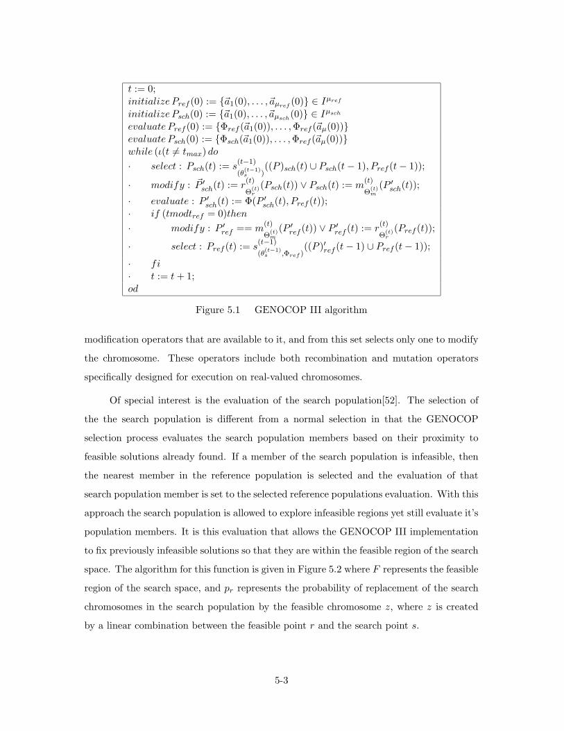
t := 0;initialize Pref (0) := ~a1(0), . . . ,~aµref
(0) ∈ Iµref
initialize Psch(0) := ~a1(0), . . . ,~aµsch(0) ∈ Iµsch
evaluate Pref (0) := Φref (~a1(0)), . . . ,Φref (~aµ(0))evaluate Psch(0) := Φsch(~a1(0)), . . . ,Φref (~aµ(0))while (ι(t 6= tmax) do
· select : Psch(t) := s(t−1)
(θ(t−1)s )
((P )sch(t) ∪ Psch(t− 1), Pref (t− 1));
· modify : ~P ′sch(t) := r(t)
Θ(t)r
(Psch(t)) ∨ Psch(t) := m(t)
Θ(t)m
(P ′sch(t));
· evaluate : P ′sch(t) := Φ(P ′sch(t), Pref (t));· if (tmodtref = 0)then
· modify : P ′ref == m(t)
Θ(t)m
(P ′ref (t)) ∨ P ′ref (t) := r(t)
Θ(t)r
(Pref (t));
· select : Pref (t) := s(t−1)
(θ(t−1)s ,Φref )
((P )′ref (t− 1) ∪ Pref (t− 1));
· fi· t := t+ 1;od
Figure 5.1 GENOCOP III algorithm
modification operators that are available to it, and from this set selects only one to modify
the chromosome. These operators include both recombination and mutation operators
specifically designed for execution on real-valued chromosomes.
Of special interest is the evaluation of the search population[52]. The selection of
the the search population is different from a normal selection in that the GENOCOP
selection process evaluates the search population members based on their proximity to
feasible solutions already found. If a member of the search population is infeasible, then
the nearest member in the reference population is selected and the evaluation of that
search population member is set to the selected reference populations evaluation. With this
approach the search population is allowed to explore infeasible regions yet still evaluate it’s
population members. It is this evaluation that allows the GENOCOP III implementation
to fix previously infeasible solutions so that they are within the feasible region of the search
space. The algorithm for this function is given in Figure 5.2 where F represents the feasible
region of the search space, and pr represents the probability of replacement of the search
chromosomes in the search population by the feasible chromosome z, where z is created
by a linear combination between the feasible point r and the search point s.
5-3

∀s ∈ Psch(t) doif s ∈ F thenΦsch(s) = Φref (s)else· r −→ Pref (r) for some r ∈ Pref· z −→ as+ (1− a)r ∈ F· Φsch(s) −→ Φref (z)· if(Φref (r) > Φref (z)) then· Pref (r) −→ z· Psch(s) −→ z|pr > rand(0, 1)· fifiod
Figure 5.2 GENOCOP III search population algorithm
The overall GENOCOP III algorithm uses a µ+1 selection, with the same operators
being used for both populations given a population size of µ. At every tref evaluations of
the search population, the members of the reference population are evolved such that if a
search population member is feasible it is included into the reference population.
The GENOCOP III complexity is directly proportional to the number of evaluations
that must be performed. Thus the algorithmic complexity for a standard EA system is
O(tmax) where tmax represents the amount of evaluations performed by the algorithm.
For the GENOCOP III system, since it uses two populations that each must be evaluated
the worst case scenario would involve a cost of t2max when the period of evolution of the
reference population is equal to one and both the reference and search populations evolve
for tmax evaluations.
5.2 Allocation EA
The primary EA that this research effort focuses on is the allocation EA. This EA
uses a specific evaluation function that allows it to search the potential solution space for
a solution. Because of the variety of factors involved with this real world problem, setting
up this EA is no trivial task. As shown in Figure 5.3, the reason the other two EA’s exist
is for tuning and evaluating the effectiveness and efficiency of the allocation EA.
5-4

Figure 5.3 The overall EA system. Note how the two coevolutionary EA’s work forimproving the results of the allocation EA.
The input for this algorithm consists of the original state of the machine So, the
relative performance characteristics of the processors % and communication links l, as well
as the task list for the next state of the machine T . With this data the algorithm computes
a next state of the system Sn such that the organization of processes to processors is an
effective mapping.
We define p to be the number of processors and m to be the number of tasks that
are being examined for each run of the allocation EA. Since it is possible that not all
processes are assigned a processor, we further define n to be the number of processes being
examined by the specific potential solution being examined, n ≤ m. Thus Pj , j ∈ 1 . . . pand Ni, i ∈ 1 . . . n represent the specific processors and tasks respectively. A state, S, is
then defined as a mapping of processors to processes such that Sk(Ni) is equal to the set
of all processors used by task Ni at time k. For the purposes of this algorithm we need
only examine two time steps, the original time k = t − 1 and the time occurring for the
new state of the system k = t.
For the request list we define Requested(i) to be the number of processors requested
by task i ∈ 1..n. Required(i) likewise represents the number of processors required by
process i. The difference between these two is substantial, as the task i must have at
least the amount of processors as given by Required(i) but should not have more than
Requested(i). Also, based on the task list we also must note whether a task can be pre-
5-5
Mela FA
C«^ L.\
|_ j ncigriimi Q J DJU
empted or not (ie can be moved between processors). Preempt(i) is given by Equation 5.1.
Preempt(i) =
0 if i preemptible
1 if i not preemptiblei ∈ 1 . . . n (5.1)
The mapping function η(Pj) is defined such that it results in the identifier i of the
task that is assigned to processor Pj , j ∈ 1 . . . p, i ∈ 1 . . . N. If η(Pj) results in 0 then
processor j is not assigned a process.
Set of Candidate Solutions. At each generation of the allocation EA a new set of
potential next state solutions are generated. The collection of these potential solutions is
the EA population. Each member of the population thus consists of an allocation scheme
for mapping the processes to the processors for the next-state of the distributed system.
If we let x represent one possible solution chromosome of the EA population then its form
would be x = x1, x2, x3, . . . , xp. Where each xi would represent the process that is allocated
to processor i.
Next-State Generator. The generation of next state candidates is done using the evo-
lutionary operators that are embedded in GENOCOP III. Being an evolutionary algorithm
it uses the genetic operators of recombination and mutation for next state generation of the
population. The difference between GENOCOP and some other EA is that GENOCOP
does not constrain itself to using just one operator. It uses a probability distribution to
choose at for each population member what type of operator is to be used, a selection from
ten potential operators that are encoded specifically for dealing with real-valued search
domains. These ten operators with their associated amount of parents and children are
listed in Table 5.1.
Uniform mutation is a basic single parent, single offspring mutation where the parent
undergoes random genetic changes to one or more of its alleles. Mathematically speaking,
given a parent x such that x = (x1, x2, x3, . . . xq), we generate x′ = (x1, . . . , x′k, . . . , xq)
where k ∈ (1, . . . , q) is chosen randomly and xk is mutated to some uniform random value
constrained within the domain of xk[51]. This creates the random diversity that allows
5-6
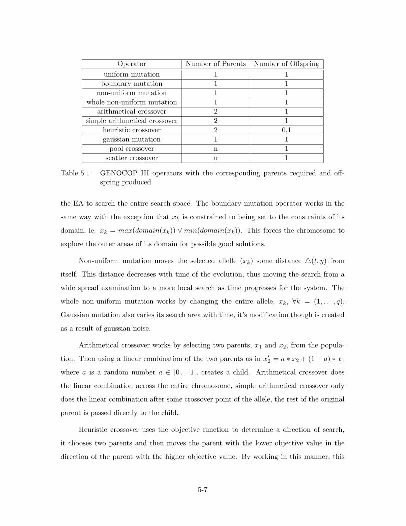
Operator Number of Parents Number of Offspring
uniform mutation 1 1
boundary mutation 1 1
non-uniform mutation 1 1
whole non-uniform mutation 1 1
arithmetical crossover 2 1
simple arithmetical crossover 2 1
heuristic crossover 2 0,1
gaussian mutation 1 1
pool crossover n 1
scatter crossover n 1
Table 5.1 GENOCOP III operators with the corresponding parents required and off-spring produced
the EA to search the entire search space. The boundary mutation operator works in the
same way with the exception that xk is constrained to being set to the constraints of its
domain, ie. xk = max(domain(xk)) ∨min(domain(xk)). This forces the chromosome to
explore the outer areas of its domain for possible good solutions.
Non-uniform mutation moves the selected allelle (xk) some distance 4(t, y) from
itself. This distance decreases with time of the evolution, thus moving the search from a
wide spread examination to a more local search as time progresses for the system. The
whole non-uniform mutation works by changing the entire allele, xk, ∀k = (1, . . . , q).
Gaussian mutation also varies its search area with time, it’s modification though is created
as a result of gaussian noise.
Arithmetical crossover works by selecting two parents, x1 and x2, from the popula-
tion. Then using a linear combination of the two parents as in x′2 = a ∗ x2 + (1 − a) ∗ x1where a is a random number a ∈ [0 . . . 1], creates a child. Arithmetical crossover does
the linear combination across the entire chromosome, simple arithmetical crossover only
does the linear combination after some crossover point of the allele, the rest of the original
parent is passed directly to the child.
Heuristic crossover uses the objective function to determine a direction of search,
it chooses two parents and then moves the parent with the lower objective value in the
direction of the parent with the higher objective value. By working in this manner, this
5-7

algorithm provides some small scale local search capability[51]. Pool crossover collects a
set of parents and mixes and matches their alleles to create a new child. Scatter also uses
a set of parents but this time it finds the central vector of the parents, it then does a
heuristic crossover operation between this central vector and the worst vector of the set,
returning the results as the child.
Selection. The selection function for both the search and reference population uses
a µ+1 approach for selecting the members of the next generation of the population. They
both use an elitist method for selecting which members of each population are to survive to
the next generation. Each time a new member is created for each population the member
is evaluated and then added into the population, the member of the population with the
lowest evaluation result is then removed from the population.
Feasibility. There are three feasibility functions that must be enforced in order to
ensure viable solutions for this algorithm. Because of the way that GENOCOP works
the solution space is constrained by these functions, but the search space does not neces-
sarily have to be. GENOCOP III allows the search to progress outside the bounds of the
constraints using a specific search population, at certain instances of the execution the pro-
gram polls this search population and moves feasible solutions to a reference population.
The final solutions are then selected only from the reference population.
The first constraint that is imposed on the solution set is a domain constraint. This
type of constraint is imposed throughout the algorithm, thus limiting the amount of search
space examined. Since each solution consists of a mapping of only N processes to the P
processors for state Sn, we must constrain η(Pj) so that it does not move beyond the
available processes as described in Equation 5.2.
0 ≤ η(Pj) ≤M ∀j ∈ 1 . . . P (5.2)
Since some processes require some upper and lower limits on the amount of processors
that they can/must support we further define the linear constraints binding them to these
limits. As explained above, Required(i) and Requested(i) define the amount of processors
5-8
that process i must have to execute and would prefer to execute respectively. Thus to
bound the amount of processors that can be used we must ensure that no more than
Requested(i) are used, and that no less than Required(i) are used.
Required(i) ≤| Sn(Ni) |≤ Requested(i) ∀i ∈ 1 . . . n (5.3)
The final constraint that must be enforced is based on ensuring that those processes
that cannot be preempted (preempt(i) = 0) are not preempted in the next state of the
system. Due to the way we set up the Preempt evaluation function (see Equation 5.1) we
can use a constraint as given in Equation 5.4.
n∑
i=1
preempt(i) ∗(
So(i)− Sn(i))
= 0 (5.4)
GENOCOP III’s approach to handling feasibility problems is based on using a repair
mechanism. The search population is allowed to explore the search space, within the
bounds of the domain constraints, without dealing with the non-linear constraints. The
reference population is kept as those solutions that meet these constraints as well. Thus
using the crossover operators as explained above the algorithm allows for exploration of
the search space outside of the constraints, but with the idea that those extraneous points
could be moved closer to the points within the feasible region through the use of a repair
mechanism. This repair mechanism chooses both a reference and a search point and creates
a line between the two. The reference point then is set to some random point along that
intersecting line. Thus moving it closer to the feasible region.
Solution. Since the GENOCOP III implementation works by storing the best solu-
tion to date from all of the potential populations, this becomes the solution result when
we are using a single objective function. This solution is selected by comparing each of the
generated population members at each of the generations to the known best solution up to
that generation. If the compared solution is better than the one stored as best then that
allele is stored as the current best solution. Since GENOCOP uses a number of generations
5-9

for calculating its results, once the a priori chosen number of generations are met then the
algorithm stops, returning the best found solution.
Objectives. For the allocation EA their are six overall objectives that were decided on
as being important for adding to the overall cost function. First off, this is a minimization
problem, the objective is to have the least total cost in terms of the overall system. How
we measure this total cost is based on the six overall objectives of: request cost (Crequest),
preemption cost (Cpreempt), processor distribution cost (Cdist), communication linkage cost
(Clink), and rollover cost (Crollover). By examining all of these we are able to put together a
cohesive objective value that represents the overall state of the system. Because of the fact
that GENOCOP III is a real-valued EA and the resulting choices are supposed to be integer
solutions, for the obvious reason that you would not have a fractional computing system,
we first truncate all of the chromosome elements (alleles) so that they can easily represent
each computer system. This is not a problem because of the fact that we constrained
the domain of the alleles to be between 0 and n + 1, therefore our possible solutions are
constrained appropriately.
The first objective that is to be dealt with is the request cost, Crequest. Each process
has some upper and lower limit on the number of processors that it can support and
that it needs to operate respectively. While these upper and lower limits create bounded
constraints on the amount of processors allocated to the process as shown in Equation 5.3
this constraint does not allow for any advantage for the process for using any more than
the lower bound of processors. Thus the request cost objective exists in order to try to
provide some benefit for using more than the lower bound of processors. For any given
process the amount of extra processors used is found using Equation 5.5.
Crequesti =| Sn(Ni) | −Required(i) (5.5)
For the cost of preemption, Cpreempt we want to minimize the overall cost of pre-
empting a process. There are two manners of preemption examined in this work: the true
preemption, that which occurs when a process is stopped so another process can use that
processor, and the preemption that occurs when a process is moved to a different processor.
5-10

Since not all processes can be preempted the feasibility of a solution based on it’s being
preemptive or not is dealt with in the feasibility section. For those processes that can be
preempted we decided to examine the two types of preemption from the perspective of
new processors added to a preexisting processor, and old processors being removed from
a preexisting process. In this manner we can examine not only the preempted processors,
but also include in it any additional cost that occurs from adding extra processors to an
already ongoing process.
For the first type of preemption, that where processes are added to a preexisting
processor, we use the cost function as given by equation 5.6.
Cpreempt+i=| Sn(Ni)− So(Ni) | (5.6)
What this equation does is give us the amount of processors that exists in the potential
next-state of the system that did not exist in the old-state of the system for the preemptible
process i. Using the same logic Equation 5.7 returns the amount of processors that existed
in the old-state of the system that are not present in the potential next-state of the system
for process i. In other words they determine the amount of processors given to and removed
from task i respectively.
Cpreempt−i=| So(Ni)− Sn(Ni) | (5.7)
The distribution cost of the processors, Cdist is a measure of the relative processing
capability of each process’s collection of processors. This is done by finding the sum squared
difference of the processor group for each process as shown in Equation 5.8.
Cdisti =
|Sn(Ni)|∑
j=1
(
%(Sn(Ni)j)−∑|Sn(Ni)|
k=1 %(Sn(Ni)k)
| Sn(Ni) |
)2
(5.8)
where, %(Sn(Ni)j) is the normalized processing capability of processor j of the set proces-
sors corresponding to the set of processes of task Ni. Hence, using this equation, we can
find, for each process, the sum squared difference between processor capability. Because
it is a squared difference we are able to extenuate those processes that have an uneven
distribution of processors.
5-11
The link cost, Clink is a measure of the overall communication overhead experienced
by each process. By using a normalized communication matrix, calculated a priori to the
EA execution, we are able to take into account all communication costs that would be
associated due to the relative node speeds, the backplane structure, etc. Thus for each
process we would calculate
Clinki=
(|Sn(Ni)|−1)∑
j=1
(|Sn(Ni)|)∑
k=j
l(Sn(Ni))jk (5.9)
as the summation of all possible communication occurrences that could occur for process
i.
The final cost chosen for examination is that of the rollover cost Crollover. This is
the cost associated with not including available processes for execution in the next-state
of the system. We find the amount of rolled-over processes using Equation 5.10. This is a
critical element of the algorithm in that we want to ensure that as few processes are not
executed as can be contained within the constraints as explained in Section 5.2
Crollover = m− n (5.10)
Now that we have identified the objectives that are incorporated into the system we
must adapt them so that they can be reasonably compared with each other. As can be
seen by Table 5.2 the domains are are too diversified to be able to be used directly in the
objective function. Also, most of the objectives only take into account a single process and
its relative configuration. Thus in order to find a unifying objective function we have to
expand our cost functions to be able to incorporate the entire system.
As before we begin with the request cost. In order to have the equation take into
account all of the different sets of processors we sum Equation 5.5 for all n. Then to nor-
malize this equation we divide by the total amount of processors that have been allocated,∑nn
i=1 | Sn(Ni) |. This provides us with a result equivalent to the percentage of processors
that this potential solution has that are over the required amount. This function, as shown
5-12
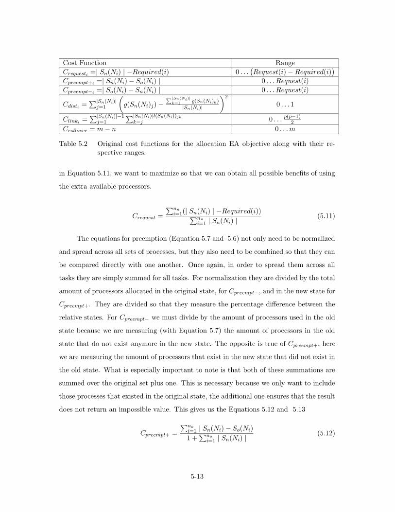
Cost Function Range
Crequesti =| Sn(Ni) | −Required(i) 0 . . .(
Request(i)−Required(i))
Cpreempt+i=| Sn(Ni)− So(Ni) | 0 . . . Request(i)
Cpreempt−i=| So(Ni)− Sn(Ni) | 0 . . . Request(i)
Cdisti =∑|Sn(Ni)|
j=1
(
%(Sn(Ni)j)−∑|Sn(Ni)|
k=1 %(Sn(Ni)k)
|Sn(Ni)|
)2
0 . . . 1
Clinki=∑|Sn(Ni)|−1
j=1
∑|Sn(Ni)|l(Sn(Ni))jk
k=j 0 . . . p(p−1)2
Crollover = m− n 0 . . .m
Table 5.2 Original cost functions for the allocation EA objective along with their re-spective ranges.
in Equation 5.11, we want to maximize so that we can obtain all possible benefits of using
the extra available processors.
Crequest =
∑nn
i=1(| Sn(Ni) | −Required(i))∑nn
i=1 | Sn(Ni) |(5.11)
The equations for preemption (Equation 5.7 and 5.6) not only need to be normalized
and spread across all sets of processes, but they also need to be combined so that they can
be compared directly with one another. Once again, in order to spread them across all
tasks they are simply summed for all tasks. For normalization they are divided by the total
amount of processors allocated in the original state, for Cpreempt−, and in the new state for
Cpreempt+. They are divided so that they measure the percentage difference between the
relative states. For Cpreempt− we must divide by the amount of processors used in the old
state because we are measuring (with Equation 5.7) the amount of processors in the old
state that do not exist anymore in the new state. The opposite is true of Cpreempt+, here
we are measuring the amount of processors that exist in the new state that did not exist in
the old state. What is especially important to note is that both of these summations are
summed over the original set plus one. This is necessary because we only want to include
those processes that existed in the original state, the additional one ensures that the result
does not return an impossible value. This gives us the Equations 5.12 and 5.13
Cpreempt+ =
∑no
i=1 | Sn(Ni)− So(Ni)
1 +∑no
i=1 | Sn(Ni) |(5.12)
5-13

Cpreempt− =
∑no
i=1 | So(Ni)− Sn(Ni)
1 +∑no
i=1 | Sn(Ni) |(5.13)
Now when combining these two objectives we have to understand that they are op-
posing objectives. In other words we want to maximize Cpreempt+ and minimize Cpreempt−.
Also, we must ensure that the objective value of adding new processors to the current
state (Cpreempt+) is not nearly good enough to cover removing processors from the original
state (Cpreempt−). This is because of the overhead cost that either adding or removing
processors to a currently executing process would incur. By adding new processors we
ensure that executing program have to send out the appropriate commands, communicate
whatever variables might be present, as well as potentially having to redistribute itself.
While this is all detrimental to the run time, overall the addition of an extra processor
should be able to benefit the executing task (assuming of course appropriate distributed
system utilization in the process). On the other hand Cpreempt− forces the processor to do
all the redistribution of load, but does not have the benefit of allowing for extra processor
utilization. Thus Cpreempt− must be weighted more than Cpreempt+. We arbitrarily chose
110 for a weight to distinguish between the two, giving us the equation:
Cpreempt = Cpreempt− −1
10Cpreempt+ (5.14)
The distribution of processing power equation Cdist is already normalized, giving
results between 0 and 1 inclusive. Equation 5.8 does not, however, calculate the total
combined power distribution of the entire graph, only of the single task i. Using the
equation for a statistical mean though fixes this nicely as shown in Equation 5.15.
Cdist =
∑nn
i=1
(
∑|Sn(Ni)|j=1
(
%(Sn(Ni)j)−∑|Sn(Ni)|
k=1 %(Sn(Ni)k)
|Sn(Ni)|
)2)
nn(5.15)
The total normalized link cost can be done in the same manner, this time dividing
by the total processing capability of the distributed system. This gives us the percentage
of communication utilized by the system. Since the linkage graph is constructed of relative
link statistics, where one represents that link being able to transmit with no relative error
5-14

and zero means that the communication link has no relative communication ability, this
equation would provide us with a statistic that increases with positive system performance.
Because we are moving towards a minimization function, we subtract this percentage from
one to have it influence the system in the manner we desire.
Clink = 1−(
∑nn
i=1
(
∑(|Sn(Ni)|−1)j=1
∑(|Sn(Ni)|)k=j l(Sn(Ni))jk
)
∑p−1j=1
∑Pk=j l(Sn)jk
)
(5.16)
Then finally the Crollover equation can be normalized by simply dividing it by the
total number of processes in the request list, m as in Equation 5.17.
Crollover =m− nm
(5.17)
Thus we can now put the overall objective equation together as a summation of the
various constituents. Since they are now normalized we can combine them in an aggregate
form with some weights to take into account the differing degrees of importance they are
towards each other. Using α1 . . . α5 for the weights then gives us the aggregate objective
as shown by Equation 5.18.
min(
α1Crequest + α2 ∗ Cpreempt + α3 ∗ Cdist + α4 ∗ Clink + α5 ∗ Crollover)
(5.18)
Of these objectives the only one that immediately stands out as needing some priority
is the cost of rollover, Crollover. We of course want to try to execute as many tasks as we
can if it is at all possible. The other objectives are related to the system performance and,
while important, are not nearly as much so as that of the rollover cost. Thus we set the
coefficient for Crollover to ten, and all of the other coefficients to one, making it one order
of magnitude larger than the others objective coefficients. The overall objective functions,
normalized so they are comparable, are given in Table 5.3.
5-15

Crequest =∑nn
i=1(|Sn(Ni)|−Required(i))∑nn
i=1|Sn(Ni)|
Cpreempt+ =∑no
i=1|Sn(Ni)−So(Ni)
1+∑no
i=1|Sn(Ni)|
Cpreempt− =∑no
i=1|So(Ni)−Sn(Ni)
1+∑no
i=1|Sn(Ni)|
Cdist =
∑nni=1
(
∑|Sn(Ni)|j=1
(
%(Sn(Ni)j)−
∑|Sn(Ni)|k=1
%(Sn(Ni)k)
|Sn(Ni)|
)2)
nn
Clink = 1−(
∑nni=1
(
∑(|Sn(Ni)|−1)j=1
∑(|Sn(Ni)|)
k=j(Sn(Ni))jk
)
∑p−1j=1
∑Pk=j l(Sn)jk
)
Crollover =m−nm
Table 5.3 Standardized objective functions for the allocation EA
5.3 Competitive EA
The competitive EA is responsible for creating a set of jobs that the allocation EA
can process. By evolving its set of requested tasks as time continues it is the goal of
this EA to generate schedules that the allocation EA would have difficulty handling. In
this manner the allocation EA can be be modified to surmount these vulnerabilities either
implicitly with the meta-EA, or explicitly through reexamination of the composition of the
allocation EA. In accordance with the biological definitions of coevolutionary organisms,
this algorithm works in an amensal relationship. This algorithms entire purpose is to create
hard schedule requests for the allocation EA, thus its objective function is inversely related
to that of the allocation EAs solution. It should be noted that since this is a dependent EA,
every time an objective function needs to be calculated a full execution of the allocation
EA must be made.
5-16

Set of Candidate Solutions. The population of this EA consists of test states with
request lists. Each chromosome is itself a state and a request list. The original state is rep-
resented in the same manner that the allocation EA represented it: x = x1, x2, x3, . . . , xp.
Where each xi ∈ Z+ represents the process that is allocated to processor i. We must also
add on the request list information concerning whether each process is preemptible, the
amount of processors required, and the amount of processors requested for each process.
We constrain the number of processes allowed to be executed to some number u. Thus
we append onto the end of the x chromosome (r−1 , r−2 , . . . , r
−u , r
+1 , r
+2 , . . . , r
+u , p1, p2, . . . , pu)
where r−i represents the amount of processors required by process i, r+i the amount of pro-
cessors requested by processor i, and pi being whether processor i is preemptible or not.
Thus for the schedule the processors requested for processor i would be the truncation of
r−i , and the processors required would be the truncation of r+i as shown in Equations 5.19
and 5.20.
Required(i) = br−i c (5.19)
Requested(i) = br+i c (5.20)
Whether or not process i is preemptible is dependent on pi is given by Equation 5.21.
preempt(i) = 0 if pi < 0.5 else 1 (5.21)
Next-State Generator. The next state of the competitive populations are produced
through the use of GENOCOP III, using the same operators as those used by the allocation
EA and explained in Section 5.2. The generator creates solutions that are viable states
with correspondingly viable request lists. The amount of processes in the state does not
necessarily have to correspond with the amount of processors in the request list so that
the allocation EA can attempt to add new processes to the state.
Selection. Since, like the allocation EA, the competitive EA uses GENOCOP III,
the selection operator is equivalent for the potential solutions. Each of the chromosomes
for this EA are weighted in proportion to their ability to maximize the objective calculated
by the allocation EA based on the schedule that each chromosome represents.
5-17

Feasibility. The feasibility of this algorithm is dependent on its own constitution.
The domain of each of xi, ∀i ∈ 1 . . . p must be between 0 and u + 1. This is needed so
that the algorithm does not produce an allocation with nonexistent processes. Along with
that, r−i and r+i must be bounded between the constraints of [1, u+1] so that they do not
ask for more processors than exist, nor less than a single processor. pi must be bounded
between [0, 1] inclusive so that it can be uniformly distributed as to whether the process
is to be preemptible.
For the non-domain constraints, the algorithm must ensure that the states it is
sending are valid. First off, if a process is in the schedule, ie for some process k, ∃xi = k,
then that process must have greater than or equal to the amount of processors it claims
to require, | S(Nk) |≥ Required(k). Also, it must have less than the amount of processes
that it requested | S(Nk) |≤ Requested(k).
Solution. A unique solution for the competitive EA is never actually found, instead
this algorithm provides a request strategy that can be used for more detailed allocation
algorithm tuning. The competitive EA runs for its specified amount of generations, at-
tacking at the objective function of the allocation EA and thus trying to help the meta-EA
optimize the allocation EA’s parameters. The only potential solution that this EA can
generate is a strategy (some chromosome) that always causes the allocation EA to have
a poor evaluation. The occurrence of this type of strategy would mean that some type
of explicit modifications to the allocation EA are necessary in order to prevent further
occurrences from happening.
Objective. The objective function of the EA is directly dependent and inversely pro-
portional to the allocation EA’s objective function. The overall goal of this research effort
is to make the allocation EA as effective and efficient as possible. Thus, since the coevolu-
tionary algorithm works as a protagonist to the allocation algorithm it wants to maximize
the overall objective value calculated for the allocation EA’s best found solution (which
again is a minimization problem). It also wants to make sure that the allocation EA has
the largest running time as possible, thus it wants to maximize the number of generations
that the allocation EA has.
5-18

Because the competitive EA has no control over the amount of generations that the
allocation EA runs, it is unnecessary for its objective function to take this into account.
That is saved for the meta-EA, as it does have control over this value. We do however
consider the objective function resulting from the allocation EA as a value for the coevo-
lutionary EA’s objective function evaluation. The objective value for the allocation EA is
defined in Equation 5.18. Using this equation we can define the allocation EA objective
as in Equation 5.22.
max(min(
α1Crequest + α2 ∗ Cpreempt + α3 ∗ Cdist + α4 ∗ Clink + α5 ∗ Crollover)
) (5.22)
5.4 Meta EA
As opposed to the competitive EA, the meta-EA has a commensal relationship with
the allocation EA. It’s objective value is directly proportional to that of the allocation
EA’s. In this manner the meta-EA’s objective evaluation improves as it is able to improve
the results from the allocation EA. The meta-EA works in the same manner as the other
evolutionary algorithms, the only difference being that it’s chromosomes determine the pa-
rameters used by the allocation EA. By doing this the algorithm evolves sets of parameters
that are optimal for the allocation EA With these parameters the meta EA fine tunes the
allocation EA so that it is able to more effectively and efficiently find solutions to whatever
allocation request is given to it.
Set of Candidate Solutions. The set of candidate solutions are the parameters nec-
essary to evolve the next execution of the allocation EA. Because, for this algorithm,
GENOCOP III is used these parameters are based directly off the input required to exe-
cute one iteration of the GENOCOP III system.
Since GENOCOP is designed as an easily configurable system the basic parameters
are inputted via an input file. The available parameters and their associated representa-
tions are listed in Table 5.4. With the exception of the number of objectives, all of these
fields are directly from the original GENOCOP III system.
5-19

Parameter Type
Number of Objectives intNumber of Variables intNumber of Non-Linear Equalities intNumber of Non-Linear Inequalities intNumber of Linear Constraints intNumber of Domain Constraints intReference Population Size intSearch Population Size intNumber of Operators intTotal Number of Evaluations intReference Population Evolution Period intNumber of Offspring for Ref. Population intSelection of Ref point for repair intSelection of Repair Method for Search Pop intSearch Point Replacement Ratio floatReference Point Initialization Method intSearch Point Initialization Method intObjective Function Type intPrecision Factor floatRandom Number Seed 1 intRandom Number Seed 2 intFreq Distribution Control Mode intDomain Constraints floatFrequency of Operators int
Table 5.4 GENOCOP III available parameters with type
5-20

Clearly not all of these fields should be altered for experimentation, and those fields
that can be altered must be bounded so that infeasible executions are not allowed to occur.
Specifically, some of the fields are held constant due to their describing the allocation EA
algorithm’s functions rather than being parameters for dealing with the search direction.
The amount of variables, type of objective, and the constraint descriptions are all held
constant throughout each run for this reason. In fact only those elements listed in Table 5.5
are able to be modified by the meta EA.
Parameter Lower Bound Upper Bound
Reference Population Size 1 1000Search Population Size 1 1000Total Number of Evaluations 1 5000Reference Population Evolution Period 1 2000Number of Offspring for Ref. Population 1 1000Selection of Ref point for repair 0 1Selection of Repair Method for Search Pop 0 1Search Point Replacement Ratio 0.0 1.0Reference Point Initialization Method 0 1Search Point Initialization Method 0 1Frequency of Operators 0 100
Table 5.5 GENOCOP III available parameters and their limits for the meta-EA execu-tion
Using the bounds as stated in Table 5.5 the meta EA creates the set of candidate
solutions by transforming these elements into a real-valued vector, which is used as the
chromosome for the meta-EA.
With these parameters being bounded as described in Table 5.5 we can find the
upper bound for the search space of the Meta algorithm. Using a floating point resolution
of 0.0001 we can define the search space to be the O(∏
Range(i))∀i ∈ param where param
defines the set of parameters being evolved.
The search space for the allocation EA is no less trivial. Because the GENOCOP
system is a real-valued algorithm the search space includes all of the floating point value
embedded in each allele. Without regard to these alleles our search space is kp where k
again is the number of tasks being run on p processors.
5-21

Next-State Generator. The next-state generation of values for this algorithm are
done using the same operators as is described earlier in section 5.2.
Selection. Selection of each chromosome occurs in the same manner as that outlined
for any other use of the GENOCOP III evaluations.
Feasibility. Other than the bounds as given by Table 5.5, the meta-EA is only con-
strained such that the reference population evolution period cannot be greater than the
total number of evaluations. The domain constraints for this algorithm are selected based
on the the maximum and minimum values found during initial experimentation.
Solution. A solution of the Meta EA is selected based on how well the allocation EA
is able to perform its task. Thus the better each of the objectives are, the more likely that
set of parameters is going to be included in the solution set.
Since the meta-EA works in a Pareto multiobjective manner each potential solution
cannot be examined without respect to the other potential solutions in the population.
Only by examining itself against these other solutions can we measure whether or not this
solution is nondominated. Those solutions that are nondominated are selected as being
the final solutions of the algorithm.
Objective. There are two objectives that the meta-EA tries to accomplish. The first
objective deals with the effectiveness of the program that it is controlling. In this respect
the meta EA wants to minimize the objective solution produced by the aggregate allocation
EA. The second objective deals with the efficiency of the program it is controlling, for
this the meta-EA works to minimize the amount of calculations necessary to produce a
solution. Since the choice of which objective we want to use is dependent on requirements
of the system a Pareto multiobjective approach is used for this algorithm, as seen in
Equation 5.23. With this type of approach we can examine what the tradeoffs between the
efficiency and effectiveness of this algorithm are. Because the results are given in a Pareto
nondominated fashion, the decision makers, are able to choose the chromosome that most
5-22

suits the research area for implementation of this algorithm.
PFknown = (min(AllocationObjective),min(AllocationComputations)) (5.23)
5.5 Combining Implementation
When in a real world application the allocation EA is expected to run as a standalone
algorithm. The meta-EA and the competitive EA are both tools designed to help improve
the allocation EA algorithm so that when it is put into the real world application it’s use
is as effective and efficient as possible. In this manner the allocation EA is designed as a
standalone algorithm that accepts for input the parameters that control its operators as
well as the request list inputted from the user via an external file that does not need to be
compiled into the algorithm itself. The meta-EA and the competitive EA work therefore to
generate these input files, the meta-EA the input file for the parameters of the allocation
EA, and the competitive EA creates the request list to be given to the allocation EA.
For each iteration of the allocation EA we are trying to find the best configuration
of processors that yields the minimum objective result as given from Equation 5.18. This
result is based off of the use of operators controlled by some set of parameters S against a
request list and previous state description R. In order to ensure that the parameters are
not evolved based on some stagnant request data, each run of the allocation EA is used
against a different R. This request list and previous state description is evolved using the
coevolutionary EA so that the allocation EA can be measured against a whole range of
potential user requests, as it would see in a real-world environment.
One approach for the overall execution of the entire allocation EA training algorithm
consists of an execution of the allocation EA once per solution generated by the coevolu-
tionary EA, and the coevolutionary EA executed once per chromosome of the meta-EA. In
this manner the results obtained by the meta-EA implicitly represent the allocation EA’s
ability to handle a spectrum of different request list possibilities.
If we allow tea to be the total amount of evaluations for the allocation EA, tem the
total amount of evaluation for the meta EA, and tec the total amount of evaluations for the
competitive EA. Then using the notation that Φa,m,c is the objective evaluation for the allo-
5-23

cation EA, meta-EA, or competitive EA respectively as given by Equations 5.18, 5.23, 5.22,
then the total algorithm execution would be as given in Algorithm 5.4
for(i = 1 . . . tem)do· Φm(~ai) = minCoev − EA :· for(j = 1 . . . tec)do· Φc(~aj) = maxAlloc− EA :· for(k = 1 . . . tea)do· Φa(~ak)· od; · od; od;
Figure 5.4 Full coevolutionary execution approach.
Unfortunately this approach is too costly in terms of overall execution time. Because
of the triple loop the cost in terms of evaluations is O(tem ∗ tec ∗ tea). For execution of
either the competitive EA or the meta-EA the best case cost is at most tem ∗ tea and
tem ∗ tea respectively.
Thus a better approach to the meta-EA is to use a small set of competitive solutions
in order to evaluate the meta-EA chromosomes. By using this approach the meta-EA tests
directly its parameter control onto highly evolved problems. With this manner and as long
as the set of chromosomes is less than tec then the overall execution time substantially less
than the triple algorithm approach.
5.6 Meta-Level Parallelization
A parallelized EA has the advantage that it can search multiple points of the search
space simultaneously. By doing this the algorithm can search more areas of the search space
in less time than would otherwise be possible, thus increasing the speed of the algorithm.
Parallelization also has the advantage that by transferring potential solutions between
different parallel populations the algorithm can maintain a high degree of diversity, thus
decreasing the chances of premature convergence [69]. There exists a variety of parallel
implementations available for parallelizing EA’s, Appendix F provides a quick explanation
of the three basic approaches.
5-24

When deciding which parallel methodology should be implemented on the GENO-
COP architecture we must examine both the network that it is to be run on as well as
the manner that the GENOCOP III system works. Between the three choices (micro-
grained, fine-grained, and coarse-grained) we can right away see the infeasibility of the
micro-grained approach. Since GENOCOP is a µ+ 1 system the evaluation of each chro-
mosome is done individually. Thus their is no large quantity of population members to
be evaluated in parallel. In fact, because of the way that the GENOCOP system is im-
plemented the selection occurs after each member is evaluated. Thus parallelization in
the micro-grained methodology would not give any speedup to the overall system since
the evaluation of each chromosome must be done in serial via the manner GENOCOP is
implemented.
Between fine-grained and coarse-grained implementations, since the topology that
this is intended to be run on is a mesh connection either approach would be relatively
easy to implement in that with either manner it is relatively simple to have each processor
communicate with those nearest it. As far as the fine-grained EA being composed of
only a single population, it can be shown that this type of system is equivalent to a
multi-population distributed EA and that only the method of communication is what
distinguishes the fine-grained approach from the coarse-grained approach [10]. Thus we
must decide upon which approach to select based solely on there relative advantages and
disadvantages of each approach and the manner for which the GENOCOP system is already
implemented.
Since GENOCOP is already implemented serially it is easy to convert it into a coarse-
grained model, with asynchronous communication amongst the populations. Due to the
proven effectiveness of this type of model for a variety of applications [10] we chose to
implement in this manner.
The parallelized GENOCOP III implementation is designed to explore the vast search
landscape of the parameters for a sub-level EA. The sub-level EA is used to generate an
allocation of processes to processors within a distributed system. This is a relatively fast
EA, and thus does not need to be parallelized. The meta-EA on the other hand can benefit
from the extra search capability that parallelization provides.
5-25

As is shown in Table 5.1, the GENOCOP III system is a complex system, but in
accordance with Appendix F, EA’s are highly parallelizable. Our implementation of the
GENOCOP III system on a parallelized platform is algorithmically similar to Algorithm 5.1
only with the added refinements of communication of the best reference vector found
by each algorithm such that it can be incorporated into the search population of those
algorithms executing relatively near the communicating algorithm as shown in Figure 5.5.
t := 0;initialize Pref (0) := ~a1(0), . . . ,~aµref
(0) ∈ Iµref
initialize Psch(0) := ~a1(0), . . . ,~aµsch(0) ∈ Iµsch
evaluate Pref (0) := Φref (~a1(0)), . . . ,Φref (~aµ(0))evaluate Psch(0) := Φsch(~a1(0)), . . . ,Φref (~aµ(0))while (ι(t 6= tmax) do· recieve : Psch −→ Psch ∪Π(i)
· select : Psch(t) := s(t−1)
(θ(t−1)s )
((P )sch(t) ∪ Psch(t− 1), Pref (t− 1));
· modify : ~P ′sch(t) := r(t)
Θ(t)r
(Psch(t)) ∨ Psch(t) := m(t)
Θ(t)m
(P ′sch(t));
· evaluate : P ′sch(t) := Φ(P ′sch(t), Pref (t));· if (tmodtref = 0)then
· modify : P ′ref == m(t)
Θ(t)m
(P ′ref (t)) ∨ P ′ref (t) := r(t)
Θ(t)r
(Pref (t));
· select : Pref (t) := s(t−1)
(θ(t−1)s ,Φref )
((P )′ref (t− 1) ∪ Pref (t− 1));
· transmit : π(Pref (i))where i is a pareto nondominated vector ∈ Pref· fi· t := t+ 1;od
Figure 5.5 GENOCOP III parallelized algorithm
In this algorithm π represents the transmission function whereby a single vector is
transmitted to the populations with a rank one above and below the population calling π.
Π represents the receiving function, whereby the search population receives a chromosome
transmitted from one of its regional neighbors and stores it to be used in its search popu-
lation. By storing in the search population the algorithm uses that new vector for moving
points that are potentially infeasible to what could be a feasible region. It also allows for
a larger use of the new chromosome for motivating the population to explore new areas of
the search space.
5-26

The complexity of this algorithm is O(t2max) number of evaluations for a worst case
scenario where the reference population is enumerated at every iteration of the search
population. We must be most concerned about the evaluations as they are the typical
bottleneck in an evolutionary algorithm [52]. Analysis of the evaluation operator for this
algorithm is difficult because of the two separate evaluation operators being executed. For
this experiment the high level meta evaluation operator is based on the best results of an
allocation EA run.
Each meta-EA execution runs a full modified GENOCOP III execution of the al-
location EA for optimizing the objectives defined therein. Thus, since the allocation EA
has a worst case scenario of O(t2max(Allocation)), the meta-EA would then have a cost of
t2max(Meta) ∗5∗ t2max(Allocation) or t4max. Thus any manner we can reduce the amount of eval-
uations necessary for the algorithm would have a dramatic effect on the overall algorithm
performance.
Since, as for any algorithm, we want to reduce the possible search space of the
problem we use the bounds as stated in Table 5.5 to bound the execution of the allocation
EA and thus the chromosome values generated by the meta-EA. A fuller description of the
parallelization of the GENOCOP system is given in Appendix G.
5.7 Summary
This chapter covers the development of the allocation EA, the competitive EA, and
the meta-EA. Each algorithm is explained with respect to its set of candidate solutions,
selection operator, feasibility constraints, solution operator, and objective evaluations. The
implementation of the modified GENOCOP III algorithm is also covered with the benefits
it provides. With the overall algorithm developed so that it meets the requirements of the
problem domain, experimentation can progress for analysis of the effectiveness.
5-27

VI. Design of Experiments
The first step to ensuring that the algorithmic approach developed here executes properly
for a real world system is to test the validity of its individual components. The test-
ing involves both the single objective and the multiobjective optimization routines of the
modified GENOCOP III system. Once it is determined that all of the algorithm imple-
mentations execute as desired, experiments can ensue that focus on the evolution and
improvement of the allocation EA.
The primary goal of the experiments is to test and adapt the allocation EA so that
it executes as effectively and efficiently as possible. To do this an examination of all of the
coevolutionary components must be performed so as to validate their support of allocation
EA. This done, the allocation EA itself can be run and optimized accordingly. It should
be noted that the allocation EA is designed to such that it executes with both efficiency
and effectiveness objectives, the supporting algorithms’ only objective is to execute for
effectiveness.
The first step is to validate the GENOCOP III’s code for effectiveness. As far as
the single objective validation is concerned, its effectiveness has previously been examined
by the system’s original designers [50]. Since this research investigation has modified the
originally single objective system to incorporate multiple objectives a validation that the
multiobjective additions execute appropriately must occur. Being that this analysis is the
foundation for the rest of the work done for this research investigation it is included in
Appendix E.
For all of this work standard statistical analysis equations of mean, median, max,
min, variance, and standard deviation are used. The student T-tests are also used in
order to compare the means of different results using the standard principles of statistical
hypothesis testing[53]. Other metrics used include spacing and ONVG for multiobjective
problem Pareto front comparisons, as explained in Appendix E. These metrics altogether
help us to examine the effectiveness and efficiency of the different algorithms being used.
While they are not the only metrics available for use in examining Pareto fronts, they
provide enough knowledge in order to understand the overall composition of the results.
6-1

This is sufficient since we are not comparing these results against other Pareto fronts, but
rather are merely trying to understand the comparative objectives.
This chapter focuses on experiments for the development and improvement of the
allocation EA. The experiments for testing the allocation EA, competitive EA, and the
meta-EA are discussed in Section 6.1. The first algorithm that is examined is the compet-
itive EA in Section 6.2. The next section then progresses to the meta-EA for optimization
of the allocation EA parameters. Finally an examination for incorporating a local-search
heuristic into the allocation EA is done in Section 6.4.
6.1 Objective/ Feasibility Testing
Since the GENOCOP III system is being used for implementation, it is unnecessary
to revalidate the single objective algorithm on benchmark problems as this algorithm has
already been tested and validated on multiple applications [50]. It is however necessary to
ensure that whatever code added to the program works as intended. All of the different
implementations have both objective function evaluators and feasibility operators that are
developed for each of the algorithms. Each section of these operators must be tested in
order to ensure that the output from each objective/feasibility operation is correct.
The only metric needed for these experiments is the objective being examined. A
simple comparison of the objectives being produced as a result of each test case to the
expected result of these cases is done in order to validate that the objective calculations
work as intended. For constraint validation a test on the results of the constraint compu-
tation on the bounds of the constraint requires the same basic computation comparison as
presented for the objectives.
Allocation EA. The allocation algorithm has multiple objectives which each must be
tested to ensure that they are outputting valid results. Validation of the different objective
calculations entails generating test cases that can test the bounds of each of the objectives
then testing the feasible region to ensure that the results calculated are equivalent to what
is expected.
6-2

Meta-EA. The objectives for the meta-EA are simple to calculate and validate. Since
the first objective is the same as that corresponding from the output of the allocation EA,
a simple examination comparing the objective result of the allocation EA and the result
stated by the meta-EA validates it’s accuracy. The second objective, being the length of
time that the allocation EA executed, is only slightly more computationally intensive. Since
the meta-EA controls the parameters being tuned, it calculates this efficiency objective by
simply examining the amount of evaluations that are done. As for the feasibility operator
for the meta-EA, since the only constraint is that the evolution period is less than the size
of the reference population it is easily validated by examination.
Competitive EA. As with the meta-EA’s first objective, the objective for the com-
petitive EA is determined via examination of the allocation EA’s solution. In order to
validate the constraints of this algorithm we generate test cases that are in the infeasible
region and ensure that the program appropriately repairs the solutions.
6.2 Coevolutionary Design of Experiments
Once the objective functions are validated so as they return appropriate results the
experimentation using the overall algorithms can be done. The first set of experiments
involve generating trials that can be used against the allocation EA. To do this, we use the
competitive EA. This algorithm’s objective is to generate difficult test problems for that
are to be used by the allocation algorithm. The reasoning behind these problems again
is to create a set of test cases for which the allocation EA can be run against that could
model real-world load-balancing scenario’s that other algorithms might have difficulties
solving (see Chapter 5.3).
Our first experiments then are to test the effectiveness of this algorithm. Thus, the
following hypothesis:
Hypothesis 1 The results generated by a competitive coevolutionary algorithm can provide
test cases that have more difficult solutions than those derived from a random generation.
H0 : µΦ(coev[1])..Φ(coev[m]) = µΦ(rand[1])..Φ(rand[m])
6-3

Test Case Number Processors Number Processes1 16 42 64 163 128 16
Table 6.1 Number of processors and processes for testing
H1 : µΦ(coev[1])..Φ(coev[m]) > µΦ(rand[1])..Φ(rand[m])
where geno[i] represents the solution found for the ith experiment with the coevolutionary
algorithm and rand[i] represents the ith random solution found for some m experiments.
The intent of this experiment is that with these ”harder” problems we can more effectively
tune the parameters of the allocation EA.
For this experiment we generate three test cases as given in Table 6.1. These test
cases were chosen because they provide three different sizes of problems for the allocation
EA to use. The 16 processor, 4 process problem is the easiest, and the 128 processor 16
process is the most complex with respect to the amount of processors/processes that is
examined by allocation EA. Due to the necessary generality of the program their is no
constraint to the size of the problem that can be generated by changing either the amount
of processors or the amount of processes (or both). The problems selected in Table 6.1
are chosen based on their varied combination of processor sizes based on real-world system
configurations with differing amounts of processes, this allows for a comparison on the
scalability of the algorithm. These values are indicative of configurations that would be
used for research environments similar to those listed in Appendix A.
As described in section 5.1, the GENOCOP III algorithm has an algorithmic com-
plexity of O(t2max). When doing a coevolutionary approach where for each evaluation a
full execution of a sub-level EA is performed, as done with both the competitive and meta-
EA’s, the algorithmic complexity moves to O(t4max). Because of this extended runtime
requirement each of these experiments is run 5 times and solutions are generated. These
solutions are each measured based on the allocation evaluation found for that solution.
The results of these evaluations are then compared statistically to equivalent executions
of a uniformly random problem generator. The statistical mean and variance is compared
using a student T-test to statistically compute the results of the hypothesis test as stated.
6-4

Parameter Value
Reference Population Size 20Search Population Size 20Total Number of Evaluations 200Reference Population Evolution Period 100Number of Offspring for Ref. Population 20
Table 6.2 Coevolutionary EA parameters for execution
The focus for this algorithm is on effectiveness and not necessarily efficiency. For
this reason we can set the parameters of the competitive EA so that it effectively generates
results without too much regard for efficiency. For this algorithm we allow for self adap-
tation of the operators using the GENOCOP III’s built in adaptation control. Since the
goal is effectiveness the experiment does not need to be overly tuned, rather just executed
for results, thus the following parameters shown in Table 6.2 have been selected for this
algorithm. Our parameter selection is made based on initial experimentation with these
parameters.
Alternatively the parameters for this algorithm are able to be set to whatever can
generate results in a realistic time frame. Since the GENOCOP III reference population
is supposed to be background operator with only infrequent evolution periods we set that
parameter to half of the total number of evaluations. The population sizes and number of
offspring is then set to 10 percent of the overall number of evaluations. Experiments even
with this parameter settings can take extensive amounts of time, especially when dealing
with larger problem sizes.
6.3 Meta EA Design of Experiments
While the meta-EA controls the parameters of the allocation algorithm, it itself need
only to operate effectively. The overall execution time of the algorithm is important only
with respect to the amount of time available for experimentation. In this manner the overall
parameters must be constrained to some limiting factor based on the lack of infinite time
to run this algorithm. Thus the meta-EA itself is set to run using the parameters as given
by Table 6.3. These parameters were chosen for the same reasons as those selected for the
competitive algorithm with the exception of the increased amount of reference population
6-5

Parameter Value
Reference Population Size 20Search Population Size 20Total Number of Evaluations 200Reference Population Evolution Period 20Number of Offspring for Ref. Population 20
Table 6.3 Meta EA parameters for execution
periods. This parameter is decreased so as to allow for migration between the parallel
populations (see Appendix G).
The goal of the meta-EA is to generate a set of parameters tuned for the allocation
EA in order to optimize its effectiveness and efficiency. This should help to optimize the
allocation EA so that it can run well over a variety of different potential inputs. In order
to ensure that the parameters are not being tuned for any specific problem we provide a
set of simulated load balancing challenges for which the evaluation of the allocation EA
can be measured against. Thus for every evaluation of the meta-EA’s chromosome the
objective evaluation is based on the allocation EA’s execution across test cases that range
in difficulty based on the amount of processors allocated a priori to the allocation EA’s
execution as well as the relative requests for processors by different processes. These test
cases however must be standardized across all of the different combinations of amounts of
processors and processes so that the results may be compared.
The optimal approach for developing the meta-EA parameters is simultaneously with
the competitive EA test case generation. Unfortunately, as described in Section 5.5, exe-
cuting both of these algorithms simultaneously is too cost prohibitive for these experiments.
Thus we must constrain ourselves to a standard set of problems from which the meta-EA
can compare the results of the different allocation EA runs. In this manner the following
test cases for execution by each allocation EA evaluation have been chosen:
• Empty original state- such that none of the processes have been allocated
• Missing one process- such that all but one process has been allocated
• Full state but one, with preemption- such that all of the processors but one have
been allocated with all of the processes
6-6

There are two experiments that must be done using the meta-EA. The first tests the
ability of the meta-EA to provide effective and efficient parameters for the allocation EA
algorithm. The second test is to examine the ability of the meta-EA for generating a set
of results that is effective across a range of problem sizes. With these two tests we can
validate the effectiveness of the meta-EA and generate good experimental results that can
be used as parameters for the allocation EA.
Parameter Generation Experiment. If we define Φ(meta[i]) to be the evaluation re-
sults of the allocation EA based on the meta generated parameters i, and Φ(generic[i]) be
the allocation EA results based on the ith set of generic parameters, then we can express
our meta first experiment hypothesis as:
Hypothesis 2 The Meta-EA can generate effective and efficient parameters that are sta-
tistically better than a set of parameters based on previous experiments, given some static
p amount of processors and N tasks.
H0 : µΦ(meta[1])..Φ(meta[m]) = µΦ(generic[1])..Φ(generic[m])
H1 : µΦ(meta[1])..Φ(meta[m]) < µΦ(generic[1])..Φ(generic[m])
In order to test this hypothesis we must have a set of parameters, based on generic ex-
periments and literature suggestions, that the meta-EA results can be compared against
when executed on the allocation EA[52]. Using the same ideas for parameter selection as
described in Section 6.2, which have been expanded due to the decreased algorithmic com-
plexity of the single EA execution, we use the parameters as given in Table 6.4 [12][51][52].
As is the case with the coevolutionary algorithm, the results of the meta-EA are based
on the evaluations of the allocation EA. However, the meta-EA has two objectives that
must be examined, effectiveness and efficiency. In order to make the result comparison
between the generic and the meta developed parameters as fair as possible solutions are
compared from the meta generated Pareto front that reside near the evaluation amount
that the generic parameter uses.
The experiment is run through the allocation EA 10 times each over the same system
designs as given in Table 6.1 for an empty processor problem, changing the uniform random
6-7
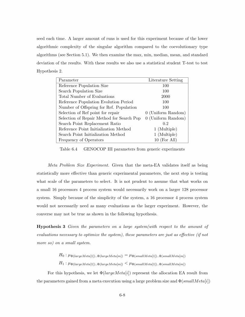
seed each time. A larger amount of runs is used for this experiment because of the lower
algorithmic complexity of the singular algorithm compared to the coevolutionary type
algorithms (see Section 5.1). We then examine the max, min, median, mean, and standard
deviation of the results. With these results we also use a statistical student T-test to test
Hypothesis 2.
Parameter Literature Setting
Reference Population Size 100Search Population Size 100Total Number of Evaluations 2000Reference Population Evolution Period 100Number of Offspring for Ref. Population 100Selection of Ref point for repair 0 (Uniform Random)Selection of Repair Method for Search Pop 0 (Uniform Random)Search Point Replacement Ratio 0.2Reference Point Initialization Method 1 (Multiple)Search Point Initialization Method 1 (Multiple)Frequency of Operators 10 (For All)
Table 6.4 GENOCOP III parameters from generic experiments
Meta Problem Size Experiment. Given that the meta-EA validates itself as being
statistically more effective than generic experimental parameters, the next step is testing
what scale of the parameters to select. It is not prudent to assume that what works on
a small 16 processors 4 process system would necessarily work on a larger 128 processor
system. Simply because of the simplicity of the system, a 16 processor 4 process system
would not necessarily need as many evaluations as the larger experiment. However, the
converse may not be true as shown in the following hypothesis.
Hypothesis 3 Given the parameters on a large system(with respect to the amount of
evaluations necessary to optimize the system), these parameters are just as effective (if not
more so) on a small system.
H0 : µΦ(largeMeta[1])..Φ(largeMeta[m]) = µΦ(smallMeta[1])..Φ(smallMeta[m])
H1 : µΦ(largeMeta[1])..Φ(largeMeta[m]) < µΦ(smallMeta[1])..Φ(smallMeta[m])
For this hypothesis, we let Φ(largeMeta[i]) represent the allocation EA result from
the parameters gained from a meta execution using a large problem size and Φ(smallMeta[i])
6-8

represents the parameters gained from a meta execution using a small problem size. In or-
der to test this hypothesis allocation EA is executed 10 times each on the afore mentioned
16/4, 64/16, 128/16 sized problems. The results are then statistically compared, again
using the standard student T test for hypothesis testing. The results are also compared
for each of the parameters for each of the problem sizes to see if they are statistically
equivalent (again using the student T-test for each). This allows a more narrow selection
of parameters that are effective/efficient for the allocation EA.
6.4 Allocation Design of Experiments
At this point the allocation EA has a ”good”, meta-EA generated, parameter set
for the to use, as well as test problems that the competitive EA generated for examina-
tion. With these the real-world effectiveness of the allocation EA can be examined. The
allocation EA is run on a variety of competitive coevolutionary EA generated problems,
as well as pedagogical problems and are examined with respect to the solution found in
comparison with a conceptual Orthogonal Recursive Bisection(ORB) algorithm. This al-
gorithm is chosen for comparison as it gives a good general solution that is known to be
quite efficient[39]. However, because of the specific choices chosen for the allocation EA
(see Chapters IV and V) comparing this algorithm to others becomes difficult at best. As
is described in Chapter III each of the different approaches must be examined with respect
to the choices made when developing the algorithm.
To further improve on the allocation EA, we compare the allocation EA’s performance
with and without a local search heuristic. The proposed heuristic is a two way sampler
that examines the generated EA chromosome for idle processors and tests the effectiveness
of running the same process that is located next to the idle processor. The algorithm then
evaluates the chromosome, finding the fitness of replacing the empty processor with either
of the processes allocated to the neighboring processors. This is a relatively simple hill
climber algorithm that has undoubtedly been used prior to this research investigation. At
this stage the algorithm has the evaluation result for the following three chromosomes:
• Original chromosome with unutilized processor.
6-9

• Modified chromosome with unutilized processor set to the same process as the lower
index processor.
• Modified chromosome with unutilized processor set to the same process as the higher
index processor.
The chromosome is then set to the process with the best evaluation of these choices. The
algorithm then proceeds to the next empty processor.
If we allow allocHC to represent the Allocation EA using the hill climber algorithm
and alloc to represent the allocation algorithm without the hill climbing algorithm then a
comparison of these two strategies can be done as shown as:
Hypothesis 4 Usage of the hill climbing algorithm statistically improves the results of the
allocation EA system.
H0 : µΦ(allocHC[1])..Φ(allocHC[m]) = µΦ(alloc[1])..Φ(alloc[m])
H1 : µΦ(allocHC[1])..Φ(allocHC[m]) > µΦ(alloc[1])..Φ(alloc[m])
In order to test this hypothesis, the experiment is run 10 times using the allocation EA
both with and without the hill climber algorithm for all three problem sizes. The results
are then compared with respect to the overall fitness, as well as the clock time necessary
to execute.
6.5 Summary
This chapter has outlined four experiments for testing the capabilities of the three
algorithms in meeting the objectives defined in Chapter I. The first experiment tests the
ability of the competitive EA to produce problems that are difficult for the allocation EA
to solve. The next two experiments are concerned with the effectiveness of the meta-EA
in generating parameters that are effective and efficient for the allocation EA. Finally, the
allocation EA is tested both with and without the use of a hill-climbing algorithm. All tests
are directed towards developing an effective and efficient allocation algorithm for processor
allocation. The results and analysis of these tests are examined in the next chapter.
6-10

VII. Results and Analysis
As is described in Chapter VI, single objective validation for the GENOCOP III algorithm
has already been accomplished[50]. The research reported here incorporates multiobjective,
multi-layer, and parallelism capabilities into this algorithm. This chapter focuses primarily
on multi-layer systems with respect to improving the performance of the allocation EA. For
further analysis, an examination of the MOP effectiveness of the GENOCOP III algorithm
is provided in Appendix E. Detailed explanations and results due to algorithm parallelism
are given in Appendix G.
This chapter follows the format of the design of experiments provided in Chapter VI.
Section 7.1 deals with the results of competitive problem generation. Section 7.2 details
findings based on the application of the meta-EA for evolving the allocation EA parameters.
Finally, Section 7.3 explains specific results of the allocation EA itself. Included in this
section is the analysis of the local search heuristic, the Pareto front objective comparison,
and a result comparison with an orthogonal recursive bisection algorithm.
7.1 Coevolutionary EA Results
The first experiment is done with the goal of validating the effectiveness of the com-
petitive EA. As can be seen from Figure 7.1 and Table 7.1 the results of the competitive
EA statistically reject our H0 from Hypothesis 1. However, this conclusion becomes ques-
tionable based on the overlap of variance shown in Figure 7.1. Ultimately the results of the
competitive need only be as good as those of the generic parameters, which they clearly are
regardless of what test is used. With further experimentation the competitive EA should
validate that it is capable of providing a strong set of test cases that are more effective
than the uniform randomly generated ones.
Parameter Type 16/4 Problem 64/16 Problem 128/16 Problem
P-value 1.3330E-4 1.24288E-2 2.44853E-3
Table 7.1 P-value for one-tailed student T-test (alpha=0.05) comparing the mean co-evolutionary result to a mean uniform randomly generated result.
7-1
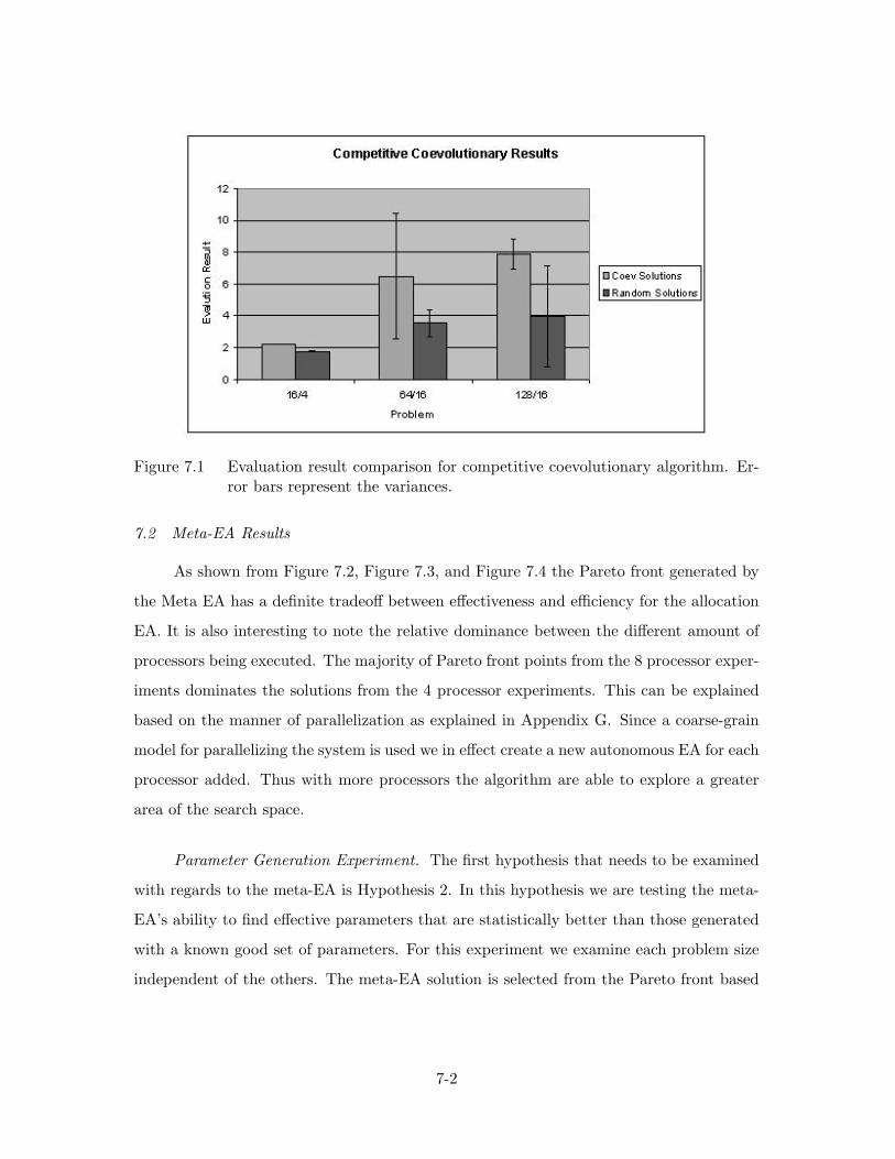
Figure 7.1 Evaluation result comparison for competitive coevolutionary algorithm. Er-ror bars represent the variances.
7.2 Meta-EA Results
As shown from Figure 7.2, Figure 7.3, and Figure 7.4 the Pareto front generated by
the Meta EA has a definite tradeoff between effectiveness and efficiency for the allocation
EA. It is also interesting to note the relative dominance between the different amount of
processors being executed. The majority of Pareto front points from the 8 processor exper-
iments dominates the solutions from the 4 processor experiments. This can be explained
based on the manner of parallelization as explained in Appendix G. Since a coarse-grain
model for parallelizing the system is used we in effect create a new autonomous EA for each
processor added. Thus with more processors the algorithm are able to explore a greater
area of the search space.
Parameter Generation Experiment. The first hypothesis that needs to be examined
with regards to the meta-EA is Hypothesis 2. In this hypothesis we are testing the meta-
EA’s ability to find effective parameters that are statistically better than those generated
with a known good set of parameters. For this experiment we examine each problem size
independent of the others. The meta-EA solution is selected from the Pareto front based
7-2
CojiweUUwe CoevoluUonvy Results
12
10
rh DC4««Salutlans
RJddoni SokiUans
lOM
PnUan
ii&ia
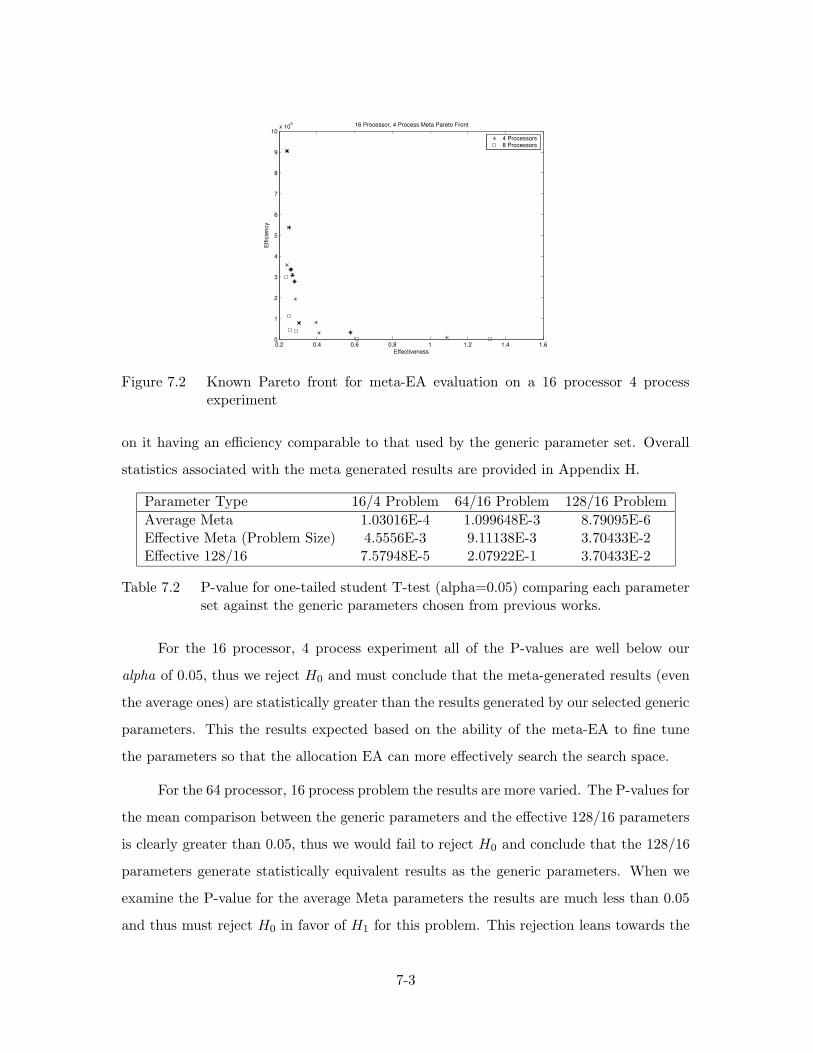
0.2 0.4 0.6 0.8 1 1.2 1.4 1.60
1
2
3
4
5
6
7
8
9
10x 105
Effectiveness
Effi
cien
cy
16 Processor, 4 Process Meta Pareto Front
4 Processors8 Processors
Figure 7.2 Known Pareto front for meta-EA evaluation on a 16 processor 4 processexperiment
on it having an efficiency comparable to that used by the generic parameter set. Overall
statistics associated with the meta generated results are provided in Appendix H.
Parameter Type 16/4 Problem 64/16 Problem 128/16 Problem
Average Meta 1.03016E-4 1.099648E-3 8.79095E-6Effective Meta (Problem Size) 4.5556E-3 9.11138E-3 3.70433E-2Effective 128/16 7.57948E-5 2.07922E-1 3.70433E-2
Table 7.2 P-value for one-tailed student T-test (alpha=0.05) comparing each parameterset against the generic parameters chosen from previous works.
For the 16 processor, 4 process experiment all of the P-values are well below our
alpha of 0.05, thus we reject H0 and must conclude that the meta-generated results (even
the average ones) are statistically greater than the results generated by our selected generic
parameters. This the results expected based on the ability of the meta-EA to fine tune
the parameters so that the allocation EA can more effectively search the search space.
For the 64 processor, 16 process problem the results are more varied. The P-values for
the mean comparison between the generic parameters and the effective 128/16 parameters
is clearly greater than 0.05, thus we would fail to reject H0 and conclude that the 128/16
parameters generate statistically equivalent results as the generic parameters. When we
examine the P-value for the average Meta parameters the results are much less than 0.05
and thus must reject H0 in favor of H1 for this problem. This rejection leans towards the
7-3
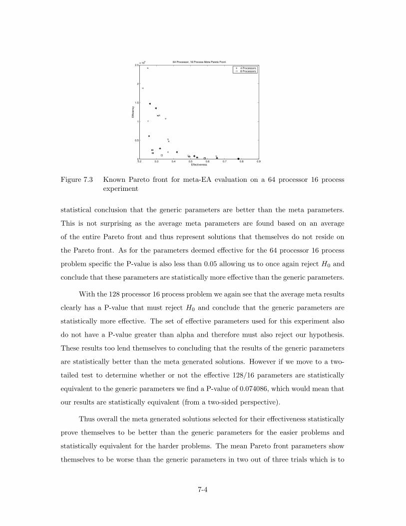
0.2 0.3 0.4 0.5 0.6 0.7 0.8 0.90
0.5
1
1.5
2
2.5x 10⁶
Effectiveness
Effi
cien
cy
64 Processor, 16 Process Meta Pareto Front
4 Processors8 Processors
Figure 7.3 Known Pareto front for meta-EA evaluation on a 64 processor 16 processexperiment
statistical conclusion that the generic parameters are better than the meta parameters.
This is not surprising as the average meta parameters are found based on an average
of the entire Pareto front and thus represent solutions that themselves do not reside on
the Pareto front. As for the parameters deemed effective for the 64 processor 16 process
problem specific the P-value is also less than 0.05 allowing us to once again reject H0 and
conclude that these parameters are statistically more effective than the generic parameters.
With the 128 processor 16 process problem we again see that the average meta results
clearly has a P-value that must reject H0 and conclude that the generic parameters are
statistically more effective. The set of effective parameters used for this experiment also
do not have a P-value greater than alpha and therefore must also reject our hypothesis.
These results too lend themselves to concluding that the results of the generic parameters
are statistically better than the meta generated solutions. However if we move to a two-
tailed test to determine whether or not the effective 128/16 parameters are statistically
equivalent to the generic parameters we find a P-value of 0.074086, which would mean that
our results are statistically equivalent (from a two-sided perspective).
Thus overall the meta generated solutions selected for their effectiveness statistically
prove themselves to be better than the generic parameters for the easier problems and
statistically equivalent for the harder problems. The mean Pareto front parameters show
themselves to be worse than the generic parameters in two out of three trials which is to
7-4
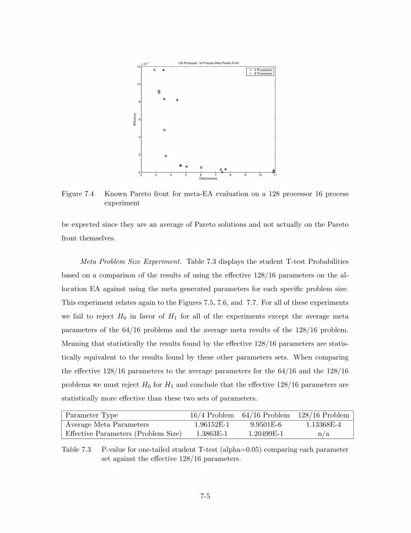
2 3 4 5 6 7 8 9 10 110
2
4
6
8
10
12x 105
Effectiveness
Effi
cien
cy
128 Processor, 16 Process Meta Pareto Front
4 Processors8 Processors
Figure 7.4 Known Pareto front for meta-EA evaluation on a 128 processor 16 processexperiment
be expected since they are an average of Pareto solutions and not actually on the Pareto
front themselves.
Meta Problem Size Experiment. Table 7.3 displays the student T-test Probabilities
based on a comparison of the results of using the effective 128/16 parameters on the al-
location EA against using the meta generated parameters for each specific problem size.
This experiment relates again to the Figures 7.5, 7.6, and 7.7. For all of these experiments
we fail to reject H0 in favor of H1 for all of the experiments except the average meta
parameters of the 64/16 problems and the average meta results of the 128/16 problem.
Meaning that statistically the results found by the effective 128/16 parameters are statis-
tically equivalent to the results found by these other parameters sets. When comparing
the effective 128/16 parameters to the average parameters for the 64/16 and the 128/16
problems we must reject H0 for H1 and conclude that the effective 128/16 parameters are
statistically more effective than these two sets of parameters.
Parameter Type 16/4 Problem 64/16 Problem 128/16 Problem
Average Meta Parameters 1.96152E-1 9.9501E-6 1.13368E-4Effective Parameters (Problem Size) 1.3863E-1 1.20499E-1 n/a
Table 7.3 P-value for one-tailed student T-test (alpha=0.05) comparing each parameterset against the effective 128/16 parameters.
7-5
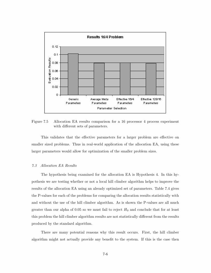
Figure 7.5 Allocation EA results comparison for a 16 processor 4 process experimentwith different sets of parameters.
This validates that the effective parameters for a larger problem are effective on
smaller sized problems. Thus in real-world application of the allocation EA, using these
larger parameters would allow for optimization of the smaller problem sizes.
7.3 Allocation EA Results
The hypothesis being examined for the allocation EA is Hypothesis 4. In this hy-
pothesis we are testing whether or not a local hill climber algorithm helps to improve the
results of the allocation EA using an already optimized set of parameters. Table 7.4 gives
the P-values for each of the problems for comparing the allocation results statistically with
and without the use of the hill climber algorithm. As is shown the P-values are all much
greater than our alpha of 0.05 so we must fail to reject H0 and conclude that for at least
this problem the hill climber algorithm results are not statistically different from the results
produced by the standard algorithm.
There are many potential reasons why this result occurs. First, the hill climber
algorithm might not actually provide any benefit to the system. If this is the case then
7-6
n -I"? -
Resurts 1614 Problem
U 1^
01 - III
S oce - III tc
0 0(6 - W
1 0(W- LU
002 -
0 -
^
1 1 1 1 1
Oenerii: A.erage Mela Etfecln.? 1&4 Ellecli.e 12&16 Parameler; Parameler; Parameler; Parameler;
Parameler Seledion
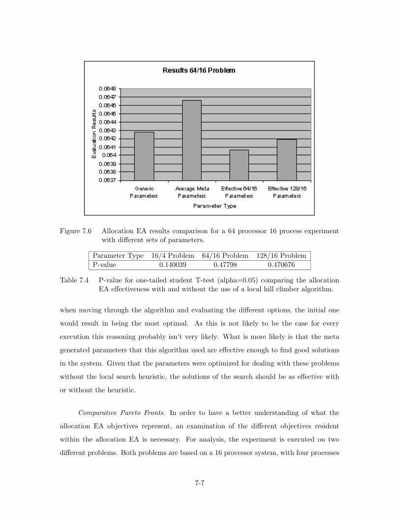
Figure 7.6 Allocation EA results comparison for a 64 processor 16 process experimentwith different sets of parameters.
Parameter Type 16/4 Problem 64/16 Problem 128/16 Problem
P-value 0.140039 0.47798 0.470676
Table 7.4 P-value for one-tailed student T-test (alpha=0.05) comparing the allocationEA effectiveness with and without the use of a local hill climber algorithm.
when moving through the algorithm and evaluating the different options, the initial one
would result in being the most optimal. As this is not likely to be the case for every
execution this reasoning probably isn’t very likely. What is more likely is that the meta
generated parameters that this algorithm used are effective enough to find good solutions
in the system. Given that the parameters were optimized for dealing with these problems
without the local search heuristic, the solutions of the search should be as effective with
or without the heuristic.
Comparative Pareto Fronts. In order to have a better understanding of what the
allocation EA objectives represent, an examination of the different objectives resident
within the allocation EA is necessary. For analysis, the experiment is executed on two
different problems. Both problems are based on a 16 processor system, with four processes
7-7
1-1 r^y>o
Resurts 64116 Problem
U Ltiti
0(647 - 0(6^6 -
^0(64^- S 0(641-
^ 0(643 - i OCC'C -
=] 0 (641 - iS 0(64-
0(6S - 0(6S - 0(637 -
1 1 1 1 1
Oeneric A..eMge Mela Ellecli"? &1/16 Etfecln.? 12&16 Parameler; Parameler; Parameler; Parameler;
Parameler Ti^e

Figure 7.7 Allocation EA results comparison for a 128 processor 16 process experimentwith different sets of parameters.
trying to execute and an assumed mesh backplane where process communication costs
between processors is directly proportional to their distances. In the first problem (Problem
1) none of the processors are initially allocated. The second problem (Problem 2) has all
of the processors initially allocated uniformly except for one empty processor. We use the
multiobjective capability of the modified GENOCOP III for enumerating the Pareto front
of the 16 processor 4 process system.
The multiobjective metrics for the different problems is given in Table 7.5. An exam-
ple of the phenotypic results of a solution of non-dominated vectors is given in Figure 7.8.
Figure 7.9 depicts the specific tradeoffs between combinations of objectives. The rollover
cost are embedded into each of the charts. Each shape represents the amount of processes
that were not included as part of the generated solution.
In order to select a load balancing configuration for a distributed system an exam-
ination of the tradeoffs between each of the different objectives is necessary. Since we
are working with a small amount of objectives we can make this comparison via graph-
ical comparisons, for a larger set of objectives a more effective method would be using
7-8
n n-ifw -
Resurts 128116 Problem
U U 1 CO
0 01S7 -
- 0 01E6 -
^ OOIES -
o 0 01S4- W 2 0 0133 - ? '" 0 01S2 -
0 OlSl -
OOIS -
1 \
I 1 1 1 1
Oeneric A..eMge Mela Elleclr..e lS/16 Etfecln.? 12&16 Parameler; Parameler; Parameler; Parameler;
Parameler Seleclion

Mean Variance Mean Variance Mean VarianceONVG ONVG Spacing Spacing Time Time
Problem 1 34.8 3.7 0.379 0.0022 80.75s 1.5833Problem 2 11.6 42.8 0.2404 0.0036 79.2 2.7
Table 7.5 Multiobjective results for the allocation problems on a 16 processor 4 processsystem
0
0.1
0.2
0.3
0.4
0
0.2
0.4
0.6
0.80.2
0.4
0.6
0.8
1
1.2
1.4
1.6
1.8
Link Cost
16 Processors, 4 Processes with 1 empty Processor
Request Cost
Pre
empt
ion
Cos
t
Figure 7.8 PFknown for a 16 processor 4 process load balancing problem. Here starsallocate all processes to processors, squares allocate all but one process, andtriangles allocated all but two processes, the circles use every processor.
a correlation analysis chart [32]. Our examination is done based on the priorities of the
intended application. The first objective that is examined for any application is that of
rollover. Regardless of the intended application, if a process is to be executed it is started
as soon as possible. Thus not including processes in the generated allocation should be
avoided if at all possible and hence our minimization of process rollovers. As can be seen
from Figure 7.9, chart C, there is clear relationship between the amount of requests able
to be satisfied and the rollover cost. This is also intuitively correct for as less processes are
executed more processors are available for the remaining processes to utilize.
Comparing the cost of communication to the amount of processes not included, it can
be seen that as less processes are included the higher the communication cost. Since fewer
processes means more processors per process the communication being higher between
these processors is understandable.
7-9

0 0.1 0.2 0.3 0.40.1
0.2
0.3
0.4
0.5
0.6
0.7
0.8
Link Cost
Req
uest
Cos
t
chart A
0 0.1 0.2 0.3 0.40
0.5
1
1.5
2
Link Cost
Pre
empt
ion
Cos
t
chart B
0 0.5 1 1.5 20.1
0.2
0.3
0.4
0.5
0.6
0.7
0.8
Preemption Cost
Req
uest
Cos
t
chart C
Figure 7.9 Comparison of specific objective tradeoffs.
When examining the request costs with respect to the other objectives it appears
that the request cost is inversely proportional to link cost (Figure 7.9A) and directly
proportional to preemption cost (Figure 7.9C). As the amount of processors allocated to
each process is increased the request cost is lowered (see Equation 5.5, but with the increase
in processors per process an increase in communication overhead occurs and hence the link
cost increases as shown by Equation 5.9. Due to the stochastic nature of the MOEA, the
allocation that is input to the system as the initial state does not imply that the result
are the same, unless the processes specifically state that they are not preemptible. Since
for this experiment all processes are assumed to be preemptible, processes are allowed to
roam from their initial configuration. From Figure 7.9, Chart C, we see that most of the
requests and preemptions lie in lower region of the objectives. Those solutions that are in
the higher area of the objective space do so for the communication cost, trading preemption
and request costs for lower link costs, as shown in Figure 7.8 and Figure 7.9, chart B.
Another important factor that should be examined that is not reflected in the objec-
tives is the amount of unutilized processors in the system. The addition of extra processors
to a process is not always beneficial, and thus should not be forced upon applications [44].
As such the addition of an extra objective for minimizing the amount of unused proces-
sors is not included. The average amount of unused processors for a Pareto front with 38
solutions is 3.94 ± 0.318 with a min of 0 and a max of 10. For the experiment presented
7-10

Figure 7.10 Allocation EA genotypic results (Pknown) of the fully utilized processors.The top row has all four processes included, the bottom row has threeprocesses included. The number and shading in each block represent theassigned process.
in Figures 7.8 and 7.9, the solutions marked with a circle represent those that utilize all
available processors. As can be seen, for this experiment, there are four solutions that
utilize all available processors. Two of these solutions allocate all of the processes, two
allocate all but one. All four points have a relatively higher request cost, which is again
explainable based on the fact that there are less processors available since they are all
being utilized. The phenotypic results are shown in Figure 7.10 where it is evident that
the processes are beginning to cluster into groups for minimizing communications.
When comparing these results to an orthogonal recursive bisection(ORB) we can see
from Figure 7.11 that the processors would be divided equally amongst the processes. This
type of allocation takes no measure of the different processor capabilities, nor does it take
into account the different communication latencies between different sets of processors.
Because the allocation EA is able to take into account all of the hardware statistics it
is able to allocate processors so that they are more efficiently located for the intended
process. This also takes into account real-world changes that could occur in the systems,
including hardware failures or heterogenous systems.
In terms of the amount of processors allocated to each process, the ORB does equally
distribute the processors among processes. If the processes then required equal amounts
of resources this would be an effective approach. However in a real-world system processes
7-11
iiiiiii 4
4 ;
1 2 12„
1 1
1114 0 missing
1 missing

Figure 7.11 Orthogonal recursive bisection genotypic results for a 16 processor, 4 processsystem.
require a varied amount of resources. With the allocation EA processes have the ability
to request ranges of processors. The amount of processors given for each process is also
encouraged towards the process’ upper limit. This allows for the processes to have the most
processors available allocated to them, while still equitably sharing the system resources.
Overall the allocation EA allows for a lot more customization per each load balancing
solution. The algorithm merges the hardware and the process information during runtime
so that it can respond to real-world developments. While the EA does not guarantee the
optimal configuration, it does allow for more thorough analysis of the system that is being
balanced.
7.4 Summary
This chapter has described the results of testing the statistical hypotheses provided
in Chapter VI. Further, since these hypotheses were developed to meet the requirements of
the initial objectives stated in Chapter I the results fulfill the stated objectives. The first
objective is met by the development and execution of the allocation EA and is validated
based on comparison to the ORB system. The second objective is fulfilled by statistical
evaluation of the coevolutionary results obtained in Section 7.1. The third and fourth
7-12

objective are met in Section 7.2 by the analysis of the meta-EA results compared to generic
and different problem size results, respectively. The final objective is met by the analysis
provided for the allocation EA using the local-search heuristic performed in Section 7.3.
Overall, the EA system is shown to perform in an effective and efficient manner, thus
allowing the generation of an effective and efficient allocation EA. ,
7-13

VIII. Conclusions and Recommendations
This research has designed and developed a load balancing algorithm that is both effective
and efficient on a variety of HPC systems. It was designed based on current load balancing
knowledge, developed so as to integrate the most current EA research, and verified using
statistical experiments. Through this process each of the goals and objectives that were
listed in Chapter I were accomplished.
For the choices that must be considered when designing an allocation algorithm for
an HPC system (as described in Section 2.1) were examined. Chapter II addressed the
choices of allocation medium, objective selection, preemption policy, process arrival rates,
a priori service demand knowledge, and process priorities. The available options, with
a general depiction of how each choice would affect the system once implemented, were
discussed for each choice. The specific problem domain for processor allocation problems
was presented in Section 2.8 to further define the problem that is the focus of this research
effort.
Chapter III examined a few of the many algorithms available for optimizing a load
balancing problem. For each algorithm, including Set Partitioning, Max-min/Min-min,
Simulated Annealing, Orthogonal Recursive Bisection, Eigenvector Recursive Bisection,
and Evolutionary Algorithms, a domain description for application to a general load bal-
ancing problem was provided. The combination of Chapter II and Chapter III fulfill the
first goal stated in Section 1.1.
Chapter IV discussed the high-level choices selected for both the problem and algo-
rithm domain. The chapter began by developing the application specific problem domain
that allows the system to be load balanced using a dynamic spatial policy. Five objectives
were selected that allow a balanced distribution of processes onto processors with regard to
the individual processor performances, the communication backplane, the process specific
preemption capabilities, and the number of processors (both required of and requested by)
each process. The problem domain was further defined to avoid expected service demand
and priority between processes.
8-1

A mapping of the problem domain to an algorithm domain was performed in Sec-
tion 4.2. This mapping allowed the implementation of both hardware and software con-
siderations. For hardware information the algorithm inputs comparative processor per-
formances and intra-processor communication capacities. For process information the
algorithm inputs a current state of the system based on the allocation of processes to
processors, the requested addition and/or removal of any process to the system with the
corresponding number of processors requested and required for execution and the possibil-
ity of preemption.
Using this mapping, Evolutionary Algorithms were selected for problem optimization.
Section 4.3 describes the three different EAs which include two coevolutionary EAs for fine
tuning the allocation EA. The first algorithm examined in Chapter IV is the allocation EA,
which uses the mapping from the load balancing problem domain to the algorithm domain
to find solutions. The first coevolutionary EA is a competitive EA designed for generating
more difficult than random problems. The other coevolutionary EA is the meta-EA which
generates a fine-tuned set of parameters that the allocation EA can use across a range of
problem sizes.
Chapter V further defined the algorithm implementations developed in Chapter IV.
These chapters fulfill the second goal in Section 1.1. Chapter V began with an explanation
of the GENOCOP III algorithm and its modifications, including the capability to optimize
Pareto multiobjective problems, to execute coevolutionary problems, and to incorporate
the parallelization technique used by the meta-EA.
The operations of the allocation, competitive, and meta algorithms were defined
with respect to their objectives, feasibility operators, selection functions, and solution
operator. The objective functions used for evaluating the allocation EA solutions for both
single and multiobjective instantiations were described mathematically in Section 5.2, and
their importance to the optimization of the system was explained. The objectives for the
other two algorithms were related to the allocation EA, as required for coevolutionary
algorithms. Section 5.6 described the reasoning behind the selection of the coarse-grained
parallelization technique applied for the meta-EA.
8-2
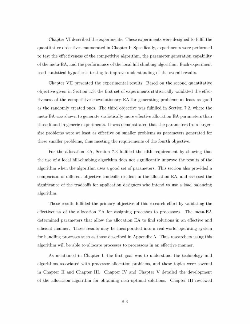
Chapter VI described the experiments. These experiments were designed to fulfil the
quantitative objectives enumerated in Chapter I. Specifically, experiments were performed
to test the effectiveness of the competitive algorithm, the parameter generation capability
of the meta-EA, and the performance of the local hill climbing algorithm. Each experiment
used statistical hypothesis testing to improve understanding of the overall results.
Chapter VII presented the experimental results. Based on the second quantitative
objective given in Section 1.3, the first set of experiments statistically validated the effec-
tiveness of the competitive coevolutionary EA for generating problems at least as good
as the randomly created ones. The third objective was fulfilled in Section 7.2, where the
meta-EA was shown to generate statistically more effective allocation EA parameters than
those found in generic experiments. It was demonstrated that the parameters from larger-
size problems were at least as effective on smaller problems as parameters generated for
these smaller problems, thus meeting the requirements of the fourth objective.
For the allocation EA, Section 7.3 fulfilled the fifth requirement by showing that
the use of a local hill-climbing algorithm does not significantly improve the results of the
algorithm when the algorithm uses a good set of parameters. This section also provided a
comparison of different objective tradeoffs resident in the allocation EA, and assessed the
significance of the tradeoffs for application designers who intend to use a load balancing
algorithm.
These results fulfilled the primary objective of this research effort by validating the
effectiveness of the allocation EA for assigning processes to processors. The meta-EA
determined parameters that allow the allocation EA to find solutions in an effective and
efficient manner. These results may be incorporated into a real-world operating system
for handling processes such as those described in Appendix A. Thus researchers using this
algorithm will be able to allocate processes to processors in an effective manner.
As mentioned in Chapter I, the first goal was to understand the technology and
algorithms associated with processor allocation problems, and these topics were covered
in Chapter II and Chapter III. Chapter IV and Chapter V detailed the development
of the allocation algorithm for obtaining near-optimal solutions. Chapter III reviewed
8-3
different algorithms associated for this problem domain, meeting the goal of examining
the allocation algorithm with respect to other available algorithms. This goal was further
completed by the comparison to the ORB algorithm performed in Chapter VII. The goal
for generating a test suite was accomplished using the competitive EA, and the final goal
of improving allocation EA performance in both effectiveness and efficiency was met using
the meta EA. Both algorithms were explained throughout development and were validated
in Chapter VI and Chapter VII. Through the fulfillment of these goals an effective and
efficient allocation algorithm was developed, thus meeting the overall goal of this research
investigation.
With the effective and efficient allocation algorithm researchers can maximize their
use of high performance computing resources. Since the algorithm is made to support any
generic HPC system it is capable of being used for a variety of applications from digital
signal processing through discrete event simulations. The algorithms ability to support
operations is not limited to the military either, homeland security efforts for real-time
aerosol and gas-hazard prediction, using real-time weather data would be supported with
this system in the same manner as the Air Force digital signal processing efforts[63].
Recommendations for Future Work
The primary future addition to this research effort would be the incorporation of
temporal allocation in addition to spatial allocation. The work presented here requires the
operating system to signal when a change to the active processes has occurred. This change
could include the addition of a new process, or the elimination of a processes due to the
absence of needed processors. For either change a signal must be given to the algorithm
for it to recompute the optimal state of the system.
A more proactive approach would include the addition of temporal statistics. If the
system contained historical data that could be analyzed statistically for patterns, then
it would be able to predict possible future states of the system. Based on potential fu-
ture states, the system could execute the allocation EA to generate a solution for each
contingency.
8-4

The new algorithm would be able to run continuously either on a dedicated processor
on various idle processors in the system. If a predicted change to the system occurs, then
the algorithm would use the pre-generated solution. If a change to the system occurs that
is not predicted, the allocation would run reactively, as in the current system. In either
case the overall cost to the system would be no worse than that of the current allocation
EA. If the algorithm to makes accurate predictions on the next state of the system, the
benefits could be significant.
Further enhancements to the system would include a dynamic hardware analyzer
that would provide normalized processor and communication comparisons needed for the
allocation algorithm. With this added function the allocation algorithm could be installed
directly into an operating system. The operating system could then be fully automated
for balancing the overall HPC system processing requirements.
8-5

Appendix A. Load Balancing Applications
To appreciate the applicability of a load balancing algorithm, at least a cursory exami-
nation of potential applications is beneficial. Two algorithms selected are Department of
Defense based projects that could potentially use the load balancing algorithm for improv-
ing overall system performance. One application is digital signal processing done by the
Air Force Research Laboratory (AFRL), which uses multiple multiprocessor applications
for analyzing signal information. The other application is a large-scale warfare simulator
used by the Air Force Wargaming Institute(AFWI) for educating Air Force personnel on
Air Force doctrine.
A.1 Digital Signal Processing
The analysis of data collected from antenna and sensor arrays is a complex task that
must be done extremely fast in order to support the real-time applications that use the
data. One project that has been designed to help further the development of HPC an-
tenna/sensor analysis applications is that being done by the Common High Performance
Computing Software Support Initiative (CHSSI) with their digital Signal and Image Pro-
cessing (SIP) efforts[2]. This project examines the use of HPC systems for large scale
real-time calculations of the following scalable digital signal processing algorithms [2]:
• Space-Time Adaptive Processing (STAP)
• Multi-Target Tracking/Tracking Toolbox
• 2-D Fast Fourier Transform(FFT)
• M-to-N Data Redistribution
The SIP effort is based on the collection of data from a variety of sensor data including
including radar, sonar, images, and others. This work supports U.S. military applications
including surveillance, reconnaissance, intelligence, communications, avionics, etc [2]. Each
of these algorithms have been ported to a parallel environment in order to support the
tremendous computational efficiency that real-time processing requires.
A-1

Space-Time Adaptive Processing (STAP) STAP is a method that uses both spatial
and temporal information to identify potential targets using statistical analysis. It uses a
2-dimensional FFT filter analysis for detection of targets amongst ground clutter and other
types of interference. STAP requires an extensive number of computations in a real-time
manner using a data cube[14].
Multi-Target Tracking/Tracking Toolbox Multi-target tracking system applications
are responsible for tracking and differentiating between multiple targets based on the sensor
data. Involved in this work is the evaluation for which targets are producing which features
from the sensor data. In order to do this analysis multiple filters and sensor data inputs
are used with statistical hypothesis generation and testing in order to differentiate between
objects [20].
2-D Fast Fourier Transform (FFT) A fast fourier transform is used to locate signals
amongst a large number of interference. It is used not only in sensor analysis but also in
quantum physics, linear systems analysis, probability theory and others [24]. Since there
are so many applications that take advantage of Fourier transforms a lot of research has
been made towards the development of more efficient algorithms [58]. Implementing a
2-D FFT is even more difficult however as each FFT is calculated first in one dimension,
then a shift or matrix transpose is performed with the FFT being recalculated in the
second dimension. This produces a great deal of both communications and computations
making the parallelization difficult an the distribution across processors important for
overall efficiency [58].
M-to-N Data Redistribution M-to-N Data redistribution attempts to optimize signal
processing applications by limiting the number of remote memory accesses needed by
each processor. At each phase of the analysis the data are redistributed so that the each
processor has the optimal number of data for processing locally [23]. This algorithm
works by transforming a cyclically distributed pattern over some initial amount number
of processors (M) to a different cyclic on a potentially different (N) number of processors
[59].
A-2

All of these applications require a great deal of computing resources provided in a real-
time fashion. An effective load balancing algorithm must therefore be able to handle the
constantly changing processing requests, allowing for new requests to be quickly inserted
into the HPC system without damaging the workload of the processors that are already
active.
A.2 Discrete Event Simulation
Discrete event simulations provide users with the ability to imitate a real-world sys-
tem over a set period of time. By being discrete the system changes only at and for
regular time intervals [6]. By using a simulation approach the users are able to, relatively
inexpensively, examine the real-world system. This approach also gives users the ability
to compress or expand time as needed for analysis. There are a variety of DES systems
that model many different real-world applications in everything from computer system
networks through restaurant traffic analysis[6]. For the purposes of this paper we singled
out a specific training simulation called the Air Force Command Exercise System (ACES).
ACES is a synchronized conservative discrete event simulation used by the US Air
Force. It currently is a serial program used for air campaign planning with the objectives
of aiding users in their understanding and appreciation of [82]:
• Air Force doctrine in a theater exercise.
• The concepts of air campaign planning.
• The synergistic effect of well-integrated air, land, and sea component plans.
• The command and staff relationships involved in combined operations.
The ACES model simulates battle scenarios for which the users can apply their
strategies. In one of the ACES simulations, called Pegasus UK, seven different simultaneous
simulations are performed that involve 90 or more participants. In each of the seven
simulations the participants are further subdivided into red and blue teams. These teams
then compete against each other using the ACES application.
A-3

The simulation moves with simulated 24 hour increments where each team develops
a theater campaign plan that they intend to be deployed against their opponents. The
simulation itself provides theater maps and status reports while the players determine
strategy, logistics and their plan of attack [83].
Once the campaign plan is decided, it is input into the ACES engine. The inputs
include the air, land, and sea orders of the units that are resident within the campaign
environment. Each of these units is assigned missions that they act during the event step.
ACES then proceeds to compute the movements of the forces and the effects thereof for
the next 24 hour increment.
Using a distributed model, the ACES system can be expanded into a much larger
simulation. Currently, in the serial version all of the players must be decomposed into
small subgroups such that each must work autonomously from the other groups. With
a distributed version a larger model could be simulated, requiring multiple processors
computing scenario regions with events communicated between systems. Thus instead of a
small localized region that is independent of anything neighboring, a more real-world model
could be implemented. This larger system would provide a better simulation of real-world
multi-theater engagements where the regions must contend for the same resources, and
actions by one commander could affect the region of another.
The distributed ACES system would require communication between multiple pro-
cessors as well as the graphical user interface (GUI). This requires a great deal of control
by the processors with a variety of computations and communications being necessary at
different times throughout the scenario. With the goal being to distribute the system
such that each regionalized area can be processed as quickly as possible with transparency
between regions a load balancing algorithm must try to ensure that the processors are
utilized to their fullest throughout the engines execution.
A-4

Appendix B. Multiobjective Approaches
Multiobjective Algorithms can be decomposed into three groups based on solution selection[75].
The types are:
A Priori Preference Articulation (Decide −→ Search) The decision maker (DM) creates
a scalar cost function, turning the MOP into a single objective problem.
Progressive Preference Articulation (Search←→ Decide) Optimization occurs on a par-
tially articulated preference set. Once optimized, a final decision is chosen by the
DM based on this set.
A Posteriori Preference Articulation (Search −→ Decide) A Pareto optimized set is
generated and the DM chooses from this set.
A recent study indicates that the popularity of multiobjective evolutionary algo-
rithm(MOEA) applications has substantially increased during the last seven years [73].
During this time the a posteriori approach has been by far the prominent choice of MOEA
developers. Many of these researchers use Pareto-based selection approaches. A more
detailed examination of the most common implementations of a priori and a posteriori
algorithms helps to clarify the distinctions.
B.1 Pareto Dominance
Using the formulation as provided by VanVeldhuizen [74], a solution is said to be
Pareto dominant if for at least one objective it has a greater evaluation than the solution
it is being compared against while all other objectives are no worse than the comparative
solution. This is algorithmically described as:
Definition 1 (Pareto Dominance): A vector u = (u1, . . . , uk) is said to dominate
v = (v1, . . . , vk) if and only if u is partially less than v, i.e.,
∀i ∈ 1, . . . , k, ui ≤ vi ∧ ∃i ∈ 1, . . . , k : ui < vi. ¤
B-1

Then for all given solutions, the Pareto optimal set of solutions is found by finding
those solutions which are Pareto dominant to all other solutions. This is described as:
Definition 2 (Pareto Optimality): A solution xu ∈ Ω is said to be Pareto optimal if
and only if there is no xv ∈ Ω for which v = f(xv) = (v1, . . . , vk) dominates u = f(xu) =
(u1, . . . , uk). ¤
With these two definitions we can begin to describe the comparison between different
multiobjective comparison techniques. It should be noted that the a priori and a posteriori
techniques both find Pareto optimal solutions. The only difference between the two is that
with the a posteriori approach a full set of Pareto optimal solutions is enumerated, while
the a priori approach finds only a single solution[12].
B.2 Weighted-Sum Selection MOEA
A standard implementation of a priori multiobjective optimization techniques is the
use of a weighted-sum objective value, otherwise known as an aggregate function [16]. This
approach combines all of the objective functions (fi(x)) into a single function of the form
mink∑
i=1
wifi(x) (B.1)
where wi ≥ 0 are the weights that are applied to each objective by the decision maker prior
to the program being executed. This approach works when the decision maker has enough
knowledge of the system to be able to specify the exact weights for each objective in order
to direct the search towards the requirements desired [12]. Aggregate functions have the
advantage of being comparatively easy to implement in that they simply turn the multiple
objectives into a single objective for evaluation. The disadvantages to this approach lie in
the fact that having the appropriate system knowledge for what to make the weights prior
to execution may be difficult or even impossible to attain.
B-2
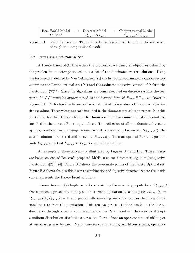
Real World Model −→ Discrete Model −→ Computational ModelP∗,PF∗ Ptrue, PFtrue Pknown, PFknown
Figure B.1 Pareto Spectrum: The progression of Pareto solutions from the real worldthrough the computational model
B.3 Pareto-based Selection MOEA
A Pareto based MOEA searches the problem space using all objectives defined by
the problem in an attempt to seek out a list of non-dominated vector solutions. Using
the terminology defined by Van Veldhuizen [75] the list of non-dominated solution vectors
comprises the Pareto optimal set (P∗) and the evaluated objective vectors of P form the
Pareto front (PF∗). Since the algorithms are being executed on discrete systems the real
world P∗,PF∗ must be approximated as the discrete form of Ptrue, PFtrue as shown in
Figure B.1. Each objective fitness value is calculated independent of the other objective
fitness values. These values are each included in the chromosomes solution vector. It is this
solution vector that defines whether the chromosome is non-dominated and thus would be
included in the current Pareto optimal set. The collection of all non-dominated vectors
up to generation t in the computational model is stored and known as PFknown(t), the
actual solutions are stored and known as Pknown(t). Thus an optimal Pareto algorithm
finds Pknown such that Pknown ≈ Ptrue for all finite solutions.
An example of these concepts is illustrated by Figures B.2 and B.3. These figures
are based on one of Fonseca’s proposed MOPs used for benchmarking of multiobjective
Pareto fronts[25], [74]. Figure B.2 shows the coordinate points of the Pareto Optimal set.
Figure B.3 shows the possible discrete combinations of objective functions where the inside
curve represents the Pareto Front solutions.
There exists multiple implementations for storing the secondary population of Pknown(t).
One common approach is to simply add the current population at each step (ie- Pknown(t) :=
Pcurrent(t)⋃
Pknown(t − 1) and periodically removing any chromosomes that have domi-
nated vectors from the population. This removal process is done based on the Pareto
dominance through a vector comparison known as Pareto ranking. In order to attempt
a uniform distribution of solutions across the Pareto front an operator termed niching or
fitness sharing may be used. Many varieties of the ranking and fitness sharing operators
B-3

−4 −3 −2 −1 0 1 2 3 4−4
−3
−2
−1
0
1
2
3
4
x1
x 2
Fonseca (2) Pareto Optimal Solutions
Figure B.2 A discretized Pareto optimal set for the MOP2 multiobjective benchmarkproblem.
exist, an examination of these algorithms is beyond the scope of this paper but the author
would refer the curious reader to [75],[17].
Once the Pareto front has been found it is then the job of the decision maker to
select which point would be best for the needs of the specific project. This makes Pareto
optimization an a posteriori technique. With proper operators this formulation can find
fully enumerated optimal surfaces for which dynamic selection at run time is available,
depending on the problem, of equally non-dominated solutions.
B-4

0 0.1 0.2 0.3 0.4 0.5 0.6 0.7 0.8 0.9 10
0.1
0.2
0.3
0.4
0.5
0.6
0.7
0.8
0.9
1
Function 1
Func
tion
2
Fonseca (2) Pareto Front
Figure B.3 A discretized Pareto optimal front, for the MOP2 multiobjective benchmarkproblem, enumerated by the *’s with the other points being feasible pointsof the search space.
B-5

Appendix C. Formalized Evolutionary Algorithms
According to Back [5] an evolutionary algorithm (EA) can be generally described as that
of Algorithm 1
Algorithm 1
t := 0;
initialize P (0) := ~a1(0), . . . ,~aµ0(0) ∈ Iµ
evaluate P (0) := Φ(~a1(0)), . . . ,Φ(~aµ(0))while (ι(P (t)) 6= true) do
· recombine : ~P ′(t) := rθr(P (t));
· mutate : P ′′(t) := mθm(P ′(t));
· evaluate : P ′′(t) : Φ(~a′′1(t)), . . . ,Φ(~a′′λ(t));· select : P (t+ 1) := sθm
((P )′′(t) ∪Q);
· t := t+ 1;
od
In order to properly understand the algorithm it is of course necessary to define the
terms used:
C-1

P Population
~ai Chromosome i of the Population
µ Parent population size
λ Child population size
Q Additional Available Individuals
Φ Fitness function
s Selection function
m Mutation function
r Recombination function
θr Recombination Parameters
θm Mutation Parameters
θs Selection Parameters
Ω Set of Probabilistic Operators
Ψ Generation Transition Function (Iµ → Iµ)
Other common operators that are employed for EA’s include chromosome decoding
operators Υ so the chromosome’s evaluation can be performed, validation operators ϑ
for ensuring the feasibility of the chromosomes, objective function f for calculating the
objective value for each chromosome, and a scaling function δ for ensuring the evaluation
results are appropriately comparable.
Using this algorithmic notation an EA is defined by its specific parameters and
operators [5]
EA = I,Φ,Ω,Ψ, s, ι, µ, λ; (C.1)
Where I is the consists of the set of elements that compose the chromosome of the EA
I = AxxAs where Ax and As are arbitrary sets that create the mapping from the problem
domain to the solution domain. The fitness function Φ, takes the chromosome and maps
it into some value that can be objectively compared (say for example a real number R)
Φ : I → R; (C.2)
C-2

This is done via the algorithm implementers selected mapping of the problem domain to
the solution domain.
The chromosomes are then modified dependent on the operators (and their associated
parameters) based on the set of available operators to the EA Ω, the most notable of which
for the purposes of evolutionary algorithms are recombination (r) and mutation (m).
Ω = ωΘ1 , . . . , ωΘz ωθi: Iλ → Iλ ∪ ωθ0 : Iµ → Iλ; (C.3)
mθm, rθr ∈ Ω; (C.4)
Mutation is formally defined as the modification of only a single chromosome without
genetic data being passed from any other chromosomes. Recombination is defined as being
the modification of one or more chromosomes based directly on the acceptance of genetic
material from other chromosomes. There are of course many different variations from
these basic genetic operators, as well as many other naturally occurring genetic operators
that have been implemented for EA’s. Some of these other operators include inversion,
conjugation, translocation, and transposition [64].
Using some combination of the genetic operators we are able to make a transition of
the EA to the next generation of the population Ψ.
Ψ(P ) = sθs(Q ∪ ωθi1
(. . . (ωθ0(P )) . . . )); (C.5)
where Q ∈ ∅, P and i1, . . . , ij ∈ 1, . . . , z. An EA must also evaluate and select from
the results. This is done with the evaluation function Φ and some selection function s.
sθs: Iλ ∪ Iµ+λ → Iµ; (C.6)
EA’s have been used for a wide variety of problem domains. They have found a
niche for themselves in solving NP-complete problems [73], including the protein structure
prediction problem [43], wire antenna designs [76] [35], load balancing [18] [7], and a variety
of other applications not to mention the ”standard” NP-complete problems like TSP [27],
C-3

Prisoners Dilemma [4], etc. In many cases EA’s are found to perform superior to other
heuristics on the same problem domain [39]. Thus making them an excellent option for
application to optimization problems.
EA Varieties
Evolutionary Algorithms themselves have evolved into a whole plethora of different
types of algorithms. Table C describes the basic elements of the most commonly used
evolutionary algorithms: Genetic Algorithms, Genetic Programs [42] [67], Evolutionary
Strategies [85], linkage learning GA’s [33] [34] and Evolutionary Programs.
Due to the fact that each of these EA heuristics are based on processes that are seen
in nature the operators that control these EA’s have a high tendency of being able to be
used in EA’s other than the those that initially utilized them. At the very least the basic
underlying biological idea, which guides the individual operators, can be modified so that
it would work in other EA’s. In this manner many of the EA’s are slowly evolving together
taking advantages of other algorithms to make themselves better. The fundamental differ-
ences in the original algorithms still exist, but the lines between the different algorithms
are slowly blurring.
These are by no means the only types of EA’s that exist. Many different versions
of these algorithms have been developed and researched. Some notable examples would
include messy genetic algorithms [29] [28] particle swarm optimization algorithm [72], ant
systems [49] [8] [70], selfish gene algorithms [19], Immune system algorithms [22] [57] and
various other types of algorithms. Each of these types differs due to some distinction it
has for changing the operators. Each class of algorithm has its own type of operator that
they claim make them unique, in general they are all of the same class of algorithms, and
can generally be used for the same overall result for problem optimization. This is not to
say that you can just pick one algorithm and it solves every problem you give it better
than any other, on the contrary the ”no free lunch” theorem [84] states that no algorithm
is best for all problems. Thus, only after a careful examination of the problem should an
algorithm be chosen, and that algorithm should be chosen based on the benefits that its
representation can bring to bear on the search.
C-4

ES [5] EP [5] GA [5] GP
Representation Real-valued Real-valued Boolean,Real, Inte-ger
Functionsand Termi-nals (string)
Fitness is Objectivefunctionvalue
Scaledobjectivefunctionvalue
Scaledobjectivefunctionvalue
Programresultsfunctionvalue
Self-adaptation
Standarddeviationsand rotationangles
None (stan-dard), vari-ances(meta),correlationcoefficients
Coevolution,vari-ances(meta)
Coevolution
Mutation Gaussian,main opera-tor
Gaussian,only opera-tor
Bit-inversion/Randomnumbergeneration,backgroundoperator
Function/terminal re-placement,subtreemutation,secondaryoperator
Recombination Discreteand inter-mediate,sexual andpanmictic,importantfor selfadaptation
Discreteand inter-mediate,sexual andpanmictic,importantfor selfadaptation
z-pointcrossover,uniformcrossover,only sex-ual, mainoperator
Tree basedcrossover,primaryoperator,usuallysexual
Selection Deterministic,extinctiveor based onpreservation
Probabilistic,extinctive
Probabilistic,based onpreservation
Probabilistic,based ontournamentor rankfitness
Constraints Arbitraryinequalityconstraints
Arbitraryinequalityconstraints
Simplebounds byencodingmechanism
Hardwareand lan-guageconstraints,feasibility.
Table C.1 Algorithmic comparison of basic EAs
C-5
Appendix D. Coevolutionary Algorithms
Coevolution in biology is the interaction of multiple species within their environment.
This principle of interacting is found throughout nature, although the interactions are not
necessarily all of the same form. Some interactions are beneficial, like the remora that
cleans parasites from shark skin. Other interactions are beneficial only one direction, like
the shark acquiring its food at the expense of other life. The interaction of each species
with other species is based on the relationship between the two species and the benefits
gained by both species.
Moving to the computational realm, coevolution can be directly applied to biological
algorithms such as EAs. By incorporating these different concepts together the engineer
hopes to gain some overall value of the system and be able to find new and improved
solutions for different problems being examined by the algorithm.
Coevolutionary Algorithms are algorithms that use the fundamentals of EAs with
multiple interacting populations each with their own unique fitness criteria to optimize
within a system. This approach involves using two or more distinct EA systems that each
have a separate evaluation function that is somehow affected by the evaluation results of
the other EA(s). In this manner both EA systems are forced to evolve together in some
type of relationship. The goal of coevolutionary algorithms is that the system evolves
solutions between the multiple algorithms that would not have been found using standard
approaches.
This appendix covers the fundamentals of coevolutionary algorithms. The different
types of relationships between algorithms is described in Section D.1. Section D.2 describes
different ways that coevolutionary Algorithms can be implemented, followed in Section D.3
where examples of implementation approaches are explained. This tutorial is not intended
to be a complete listing of all research in coevolutionary algorithms, rather it is a tutorial
with basic terminology and examples to be used as an introduction into the vast field of
coevolution.
D-1

D.1 Relations of Coevolutionary Algorithms
There are a variety of methods for classifying algorithms that are coevolutionary. A
standard approach is through the analysis of the interactions between each of the popu-
lations. This type of analysis typically uses biological definitions to classify each set of
populations based on how they work together. In order to be able to explain coherently
the computational models it is important to have a good understanding of their biological
definitions. We use the definitions presented by Morrison as the foundations for which to
build our exploration of the interactions. The basic structure for which all specific rela-
tionships are based on can be described from the first four definitions of symbiosis, and
antagonistic vs protagonistic symbiotic connections being defined as [55]:
Definition 1 (Symbiosis) Symbiosis is a relationship between two (or more) individuals
such that the fitness of one individual directly affects the fitness of the other individuals(s).
Using this definition Morrison formally restates the coevolution as [54]:
Definition 2 Coevolution of a population with itself occurs when individuals within the
population are in symbiosis with other individuals in the same population. Coevolution
of a pair of populations with each other occurs when individuals in one population are in
symbiosis with individuals of another population.
The symbiosis between any two individuals can be broken down then into a more
specific description as:
Definition 3 (Symbiotic Connection) A −→ B (A affects B) between two individuals
A and B exists if and only if the fitness of A has a direct effect on the fitness of B.
Definition 4 (A+−→ B) (A protaganizes B) if and only if there exists a connection A −→ B
such that as the fitness of A increases, the fitness of B increases, and as the fitness of A
decreases, the fitness of B decreases.
Definition 5 (A−−→ B) (A antagonizes B) if and only if there exists a connection A −→ B
such that as the fitness of A increases, the fitness of B decreases, and as the fitness of A
decreases, the fitness of B increases.
D-2
With these three definitions we can then explicitly define the different relationships
between individuals as being related to one of the following five relationships. Each of
these represent a symbiotic connection that are seen in nature, and also have practical
advantages to their being applied to optimization problems.
Definition 6 (Amensalism) occurs between two individuals, Host and Amensal, if and
only if Host−−→Amensal and ¬(Amensal−→Host).
Definition 7 (Commensalism) occurs between two individuals, Host and Commensal,
if and only if Host+−→Commensal and ¬(Commensal−→Host).
Definition 8 (Competition) occurs between two individuals, Competitor A and Com-
petitor B, if and only if Competitor A−−→Competitor B and Competitor B −−→Competitor
A.
Definition 9 (Predation) occurs between two individuals, Predator and Prey, if and only
if Predator−−→Prey, and Prey +−→Predator.
Definition 10 (Mutualism) occurs between two individuals, Symbiont A and Symbiont
B, if and only if Symbiont A+−→Symbiont B and Symbiont B +−→Symbiont A.
Using these relationship definitions each program can be expressed specifically as a
type of coevolution. With that in mind we can coherently sort the different algorithms
into respectable groupings.
D.2 Implementation of Coevolutionary Algorithms
As the coevolutionary algorithms that we are exploring are based on the normal
evolutionary algorithm substructure we can directly incorporate many of the operators
from the algorithm we have chosen. Thus the genetic evolvers such as recombination and
mutation can be the same as they were in the standard EA. There are some changes that
do have to be made in order for the algorithm to function appropriately, this is primarily
seen in the fitness evaluation of the population members.
D-3
Fitness Evaluations. Evolutionary algorithms are traditionally designed with a sin-
gle objective, single species approach. By this I mean that there is only one population
composed of like individuals (individuals that share the same encoding) that are all opti-
mized based on a single objective function. Thus if two solution vectors ~a and ~b existed
in the population such that ~a = ~b, then their evaluation in the fitness would be equivalent
(given a discrete fitness function, f(~a) = f(~b)).
In a coevolutionary algorithm this changes. The encodings might still be the same, ie
~a = ~b, but their finesses might turn out to be different based on what fitness evaluation each
vector is made to undergo, so that it is quite possible that f1(~a) 6= f2(~b). Other encodings
could have multiple different populations, each normally called a separate species. There
is a large variety of these different encoding designs, and it is important to examine the
benefits associated with each.
As there is no free lunch for normal evolutionary algorithms the same holds true
for the coevolutionary arena [84]. There is therefore a vast range of possible algorithms
which can and are applied to different coevolutionary problems. The design that is chosen
would require the engineer to understand the problem domain and apply the appropriate
biological symbiosis between the algorithms for the program to be effective.
Whereas a standard evolutionary algorithm commonly uses a discrete fitness based
solely on the evaluation of an individual. A coevolutionary algorithm commonly uses what
is known as a competitive fitness function (CFF) [3]. A CFF occurs when the fitness of
an individual is calculated based on trials where the individual is matched against other
members of the population(s). The results of these trials then move the evolution of the
population towards some optimal goal.
Different implementations of the CFF trials exist, they differ based on the selection
of the members that are being compared and are thus classified as such[56].
Definition 11 (All vs All) CFF’s match every individual from the population(s) against
every other individual [4].
D-4
Definition 12 (Random Competition) selects a fixed number of random population
members for competition against the individual being examined [60].
Definition 13 (Tournament) competition ranks the fitness of the individual by single
elimination one-to-one tournaments [3].
Definition 14 (All vs Best) competition tests the individual singly against the currently
best individual in the population [41].
This is of course not an exhaustive list as other examples of methods of selecting
competitions can be made using any selection technique, these are simply examples of the
selections done from literature.
The competitive fitness evaluation of the coevolutionary algorithm can be easily
compared to the ranking necessary for a Pareto multiobjective algorithm. In a Pareto
multiobjective algorithm the program tries to optimize multiple different objectives simul-
taneously. Since not all objectives can be optimal at the same time, a tradeoff of objective
finesses is made while maintaining that the each objective reaches their fullest possible
value given the tradeoff. To determine which solutions are best for some tradeoff each
solution vector is ranked. This ranking must examine each solution vector against ev-
ery other solution vectors relative fitness to determine its rank in the population. This
approach corresponds directly with the All vs All approach.
Population Modelling. Their are many different manners by which a coevolutionary
system can have the different population species coexist. These implementations depend
on the available computer resources, and of course on the approach by which the problem
is undertaken. The basic form of population decomposition is to use a sequential program
whereby each population is evolved to the point where interaction is necessary between
the populations. At this point the finesses are calculated and the evolution proceeds.
A simple distributed conversion of this method is to let each processor evolve the pop-
ulation till the interactive fitness calculations are made. This model is sometimes referred
to as a form of the island model of evolutionary computation because each population is
evolved in isolation with communications made infrequently between populations.
D-5

Yet another model, would be to use a distributed system where each of the pop-
ulations are spread out over a grid, interactions can then occur locally. This model is
normally labelled a fine-grain parallelization, and it has the benefit of making inter-special
communication possible within local groupings of the system [40].
D.3 Coevolutionary Algorithm Examples
The number of applications which take advantage of coevolutionary algorithms is
ever increasing. While GA’s are commonly used as the primary backbone for which the
coevolutionary structure is applied it is not uncommon for other styles of evolutionary
algorithms to be used [37].
Immune System. An Artificial Immune System (AIS) uses the fundamental elements
of a human immune system in order for optimizing systems in which some type of pattern
matching is required. Perhaps the primary realm for which AIS’s are implemented is
for computer security, for example AIS are used for Computer Virus Detection, where
computers are examined for self versus non-self items resident in the computer’s memory.
In an immune system there exist two basic units, the antigens and the antibodies.
Antigens are defined as foreign material that should not be in the body; bacteria, viruses
are two primary examples. Antibodies are the detector cells that can distinguish between
material that is supposed to reside in the body (self) and material that is foreign (anti-
gens). In each individual there are numerous different antibodies that exist, each detecting
different strains of antigens. When detection occurs the body goes through a phase called
clonal expansion by which the antibodies are duplicated in mass. This large concentration
of antibodies then overwhelms and neutralizes the antigen [21].
Another useful feature of the immune system is its memory. When antibodies undergo
a clonal expansion the body remembers what the pathogen was. Thus, if another invasion
by that antigen does occur, the body can quickly produce the appropriate antibodies to
stem the infection. In biological terms this memory is called the immunological memory.
When converting this system from the biological to the electronic these principles
become amazingly useful as an adaptive system for pattern recognition. The principles of
D-6

antibody responses and clonal expansion relate (in their simplified forms) to the matching
of patterns within a system and the dynamic creation of more strings for recognizing a
greater number of patterns. The memory of the immunological information is analogous
to the memory of the patterns. For example, in the virus detection system, immunological
information would be the history of all viruses found to date [21].
Clearly this is a realm of computer algorithms that is prime for coevolutionary adap-
tation. There are actually many different features of immune systems that can be modified
to work using a coevolutionary scheme. Perhaps the most obvious adaptation would be to
use a competition strategy between the antigens and the antibodies. In this manner the
population of antibodies would develop for better matching of the antigen strings. The
antigens would then develop for improvement on stumping the antibodies.
Another approach would be to have two populations, one of antibodies, one of helper
T-cells (or even other antibodies) Helper T-cells aid the antibodies for detecting antigens.
Using this idea the helper T-cells would develop in a mutualistic relationship with the
antibodies, providing extra data for matching the antigens.
One example of the use of a coevolutionary immune system is for evolving antibodies
for concept learning [57]. This research investigation uses a genetic algorithm and a binary
schema representation where self is the negative examples and the positive examples are
likened to antigens. The coevolutionary approach used here is implemented for the goal
of maintaining genetic diversity with multiple antibody populations and a mutualistic
collaboration. What happens is that the antibodies seek out the non-self positive learning
examples and stores the information. This continues until all the foreign molecules and
none of the self are recognized, thus having stored a full concept picture.
Genetic Programming and Predation. A classical example of a predation relationship
in biology is the relationship of a predator and prey. A simple example of a pack of wolves
hunting a deer can be used to understand the problem. Using this example the wolves,
being the predators, have the objective of capturing the deer and the deer has the objective
of escaping the pack of wolves.
D-7
One implementation of this experiment is done using a strongly typed genetic pro-
gram (STGP) [37]. A genetic program uses the biological operators (most notably that of
mutation) to generate an executable program based on a listing of terminals and functions.
The terminal set for this implementation consists of the agents in the system (both the
predators and the prey). The function set consists of commands for moving the agents
around the 2-D grid world as well functions for comparison (ie. less than and if then else
clauses).
The reason why it is a strongly typed genetic program is that all of the constants,
terminals, variables and returned values can be of any type [37]. This is done with the
use of generic functions that can accept and return data of any generic data type. The
reasoning behind this is to ensure that all operations can construct valid programs.
This problem is divided into two distinct problems. First, the problem of interaction
and cooperation of the predators is examined [37]. That is done using a prey that randomly
moves around the board without any direction. Since this is not realistic and in order to
make the problem a bit more difficult for the prey, experiments are then made for the
coevolution of the preys movements instead of the simple random movement [36].
In the first implementation the STGP moves all members of the board simultaneously.
The goal of the predator agents is to surround the prey, thus immobilizing it. The predators
are allowed to ”see” the prey, but not each other, they can however bump each other if
they try to occupy the same location on the grid. The program that is evolved is used by
all predators.
The basis for fitness of the capture strategy in this program is a weighted point
system where the highest weight is given for capturing the prey. Since it is not always
guaranteed that the prey is captured other measurements for fitness evaluation were also
included. Second to the actual capturing and encirclement of the prey was adjacency to
the prey, this made the program favor predators being close to circling the prey. Finally
the last and least weighted term was that of proximity for those that are near but not
adjacent to the prey [37].
D-8

The next generation of this program is where the real coevolutionary predation algo-
rithm occurs. The predator agents use the same method as described above for generating
programs for their decisions, but this time the prey turns from the random movement to a
decision process based on its own GP. Initial results found that the predator language had
to be expanded because the prey systems were too effective at avoiding the predator, thus
they expanded the implementation to allow them to see each other. Even this improvement
is no match for the prey’s simple yet effective evasion algorithms.
Genetic Algorithms and Symbiosis. Not all coevolutionary systems are as direct and
easy to recognize as those of the immune system (Section D.3) or the predator and prey
GP (Section D.3). Some implementations simply have two or more coexisting coevolving
populations that interact only in the workings of the program. A good example of this is
Michaelewicz’s GENOCOP III [50].
GENOCOP III is a generic genetic algorithm (GA) that uses two populations, one
for search the other for reference. The evaluation of the search population depends on
the current reference population. The reference population is the created based off of the
search population, but its evaluation is independent. This results in the system being a
commensal arrangement.
Applications of this program are extremely diverse. One application was for the de-
sign of wire-antenna design [76]. An extension of this project was also done for using Pareto
optimization along with the coevolutionary structure for finding the antenna geometries
along the entire Pareto front.
Meta-EA. Meta-EAs work differently than the standard coevolutionary system. Most
coevolutionary systems have interactions between all populations. In a meta-EA the in-
teractions only go one way, the meta-EA optimizes the operators and parameters for the
sub-EA, and the sub-EA uses these parameters and operators to optimize the problem
being examined. Using definition 2 all a system needs in order to be coevolutionary is a
fitness based on a population other than the one being evaluated. With this definition the
Meta-EA is coevolutionary and the interaction can be described as commensalism.
D-9

Perhaps the most developed research into multilayer programs was done by Gang
Wang et. al and the work done for the DAGA2 [80], [79], [81]. The DAGA2 system
optimized not only the objective being examined for some problem domain, but also the
system in which the individuals were being evolved in. They used a recursive encoding
approach, such that there could be any number of meta-level algorithms as the user wanted
to implement.
The goal of the DAGA2 project was to try to overcome the No Free Lunch theorem
[84], [80]. They had the meta-GA select the operators for selection, crossover, and mutation
and the parameters and probabilities for each. The fitness of the meta-GA was then
based on a combination of best fitness of individuals in the sub-GA, average fitness of the
individuals in the sub-GA, number of fitness function evaluations of the sub-GA, and a
measure of population diversity in the sub-GA.
The sub-GA ran with the parameters as specified by the meta-GA. It’s fitness was
based directly on the problem domain, and was not influenced by any of the results of the
meta-GA. Being that it is a one sided fitness relationship, we call it commensalism.
D.4 Summary
The coevolutionary algorithms are a powerful and diverse use of biological models for
interacting populations. The results found by coevolutionary algorithms are many times
unexpected and of higher quality than could be found with standard EAs and standard
fitnesses [37].
By using interacting populations programs are able to build on each other to find
solutions that may not have been thought of otherwise. There are a variety of different
interactions that can be used based on the system that is being modelled and the popu-
lations that are chosen to interact. Using these interactions fitnesses must be calculated
based on the performance of not only the population being evaluated but on the other
populations in the system- this is what makes it coevolutionary.
D-10
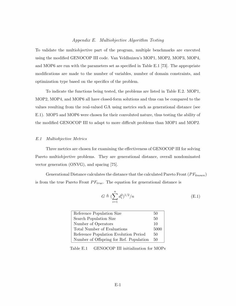
Appendix E. Multiobjective Algorithm Testing
To validate the multiobjective part of the program, multiple benchmarks are executed
using the modified GENOCOP III code. Van Veldhuizen’s MOP1, MOP2, MOP3, MOP4,
and MOP6 are run with the parameters set as specified in Table E.1 [73]. The appropriate
modifications are made to the number of variables, number of domain constraints, and
optimization type based on the specifics of the problem.
To indicate the functions being tested, the problems are listed in Table E.2. MOP1,
MOP2, MOP4, and MOP6 all have closed-form solutions and thus can be compared to the
values resulting from the real-valued GA using metrics such as generational distance (see
E.1). MOP5 and MOP6 were chosen for their convoluted nature, thus testing the ability of
the modified GENOCOP III to adapt to more difficult problems than MOP1 and MOP2.
E.1 Multiobjective Metrics
Three metrics are chosen for examining the effectiveness of GENOCOP III for solving
Pareto multiobjective problems. They are generational distance, overall nondominated
vector generation (ONVG), and spacing [75].
Generational Distance calculates the distance that the calculated Pareto Front (PFknown)
is from the true Pareto Front PFtrue. The equation for generational distance is
G , (n∑
i=1
d2i )1/2/n (E.1)
Reference Population Size 50Search Population Size 50Number of Operators 10Total Number of Evaluations 5000Reference Population Evolution Period 50Number of Offspring for Ref. Population 50
Table E.1 GENOCOP III initialization for MOPs
E-1

MOP Definition Constraints
MOP 1 F = (f1(x), f2(x)), where
f1(x) = x2,
f2(x) = (x− 2)2
None
MOP 2 F = (f1(~x), f2(~x)), where
f1(~x) = 1− exp(−n∑
i=1
(xi −1√n)2),
f2(~x) = 1− exp(−n∑
i+1
(xi +1√n)2)
−2 ≤ xi < 2
MOP3 Maximize F = (f1(x, y), f2(x, y)), where
f1(x, y) = −[1 + (A1 −B1)2 + (A2 −B2)2],f2(x, y) = −[(x+ 3)2 + (y + 1)2]
−3.1416 ≤ x, y ≤ 3.1416,
A1 = 0.5 sin 1− 2 cos 1 +
sin 2− 1.5 cos 2,
A2 = 1.5 sin 1− cos 1 +
2 sin 2− 0.5 cos 2,
B1 = 0.5 sinx− 2 cosx+
sin y − 1.5 cos y,
B2 = 1.5 sinx− cosx+
2 sin y − 0.5 cos y
MOP4 F = (f1(~x), f2(~x)), where
f1(~x) =n−1∑
i=1
(−10e(−0.2)∗√x2i+x
2i+1),
f2(~x) =n∑
i=1
(|xi|0.8 + 5sin(xi)3)
−5 ≤ xi ≤ 5; i = 1, 2, 3
MOP6 F = (f1(x, y), f2(x, y)), where
f1(x, y) = x,
f2(x, y) = (1 + 10y) ∗[1− ( x
1+10y )α − x
1+10y sin(2πqx)]
0 ≤ x, y ≤ 1,
q = 4,
α = 2
Table E.2 MOEA test functions
E-2

where n is the number of vectors found for PFknown, di is the Euclidean distance between
each PFknown vector and the closest PFtrue vector. Optimally the result of this would be
0 meaning that all vectors found are on PFtrue.
ONVG is a calculation of the amount of unique nondominated vectors found by the
algorithm. Mathematically speaking it is
ONV G , |PFknown| (E.2)
This metric helps examine how effective the algorithm is for enumerating potential solutions
that the decision maker can choose from. It gives us no information concerning if the results
are along the Pareto Front, nor if they are spaced evenly among the search area, only how
many of these vectors exist.
In order to examine how evenly spaced the solutions found are along the solutions
surface a metric called Spacing is used. The equation for spacing is
S ,
√
√
√
√
1
n− 1
n∑
i+1
(d− di)2 , (E.3)
where di = minj(| f i1(~x) − fj1 (~x) | + | f i2(~x) − f
j2 (~x) |), i, j = 1, . . . , n, d is the average for
all di. Again the smaller the value the more equidistant the points are in the found Pareto
Front, optimally we want a value of 0 for this metric.
The use of all three of these metrics allows a statistical analysis of how effective
the GENOCOP III implementation would be at finding good solutions for multiobjective
problems. From ONVG we have how many solutions are found, spacing tells us how well
distributed they are, and generational distancing tells us how good of a solution they are.
Each individually gives a small picture of the overall success, when looked at together we
have a much better picture of how effective the program is.
Statistical Techniques The benchmarks are each be run 50 times. Once run the
three metrics of generational distancing, spacing, and ONVG are applied. The mean and
standard deviation for these runs are then found. These results are then be compared
E-3

Mean Std Dev Confidence
Spacing 0.097579 0.102171 .002832
ONVG 482.98 673.608 186.7109
GD 0.015358 0.014987 0.004154
Table E.3 MOP1 metrics
with other competitive algorithms, so that a comparison of algorithm performance can be
made.
E.2 MOP Results
Each benchmark is initialized using the parameters specified in Table E.1. Each
MOP is run 50 times, and the results were stored. Metrics were then applied with results
as seen in Tables E.3, E.4, E.5, E.6, E.7.
When examining these results it is important to remember that GENOCOP III
operates with real-value results while all the found pareto optimal set is determined for
a binary representation. In this manner the results become hard to analyze due to the
inability to directly compare results.
The results of MOP1 (Table E.3) shows a good spacing across the true Pareto front.
It would be better to have the spacing a little closer to 0, but due to the fact that niching
is not applied to the program this result is understandable. The ONVG gives a reasonable
amount of points found on for our PFknown. This in reality, since we are dealing with
real a real-value EA, would be an uncountably infinite amount of points along a curve.
Figure E.1 also helps for visualizing how close the found Pareto optimal points are to
the true Pareto front. The close proximity that is seen by the graph is also displayed
through the generational distance metric. This metric is slightly biased due to the fact
that the GENOCOP III uses real valued loci and the true Pareto front is enumerated only
at discrete points, overall this metric is small enough a value to confirm that we have found
a true Pareto front.
The results of MOP2 (Table E.4) have a better spacing than MOP1. The results
here are more equally spaced along PFknown. The ONVG would also be an uncountably
infinite number for this problem due to the real-valued implementation. Once again, the
E-4
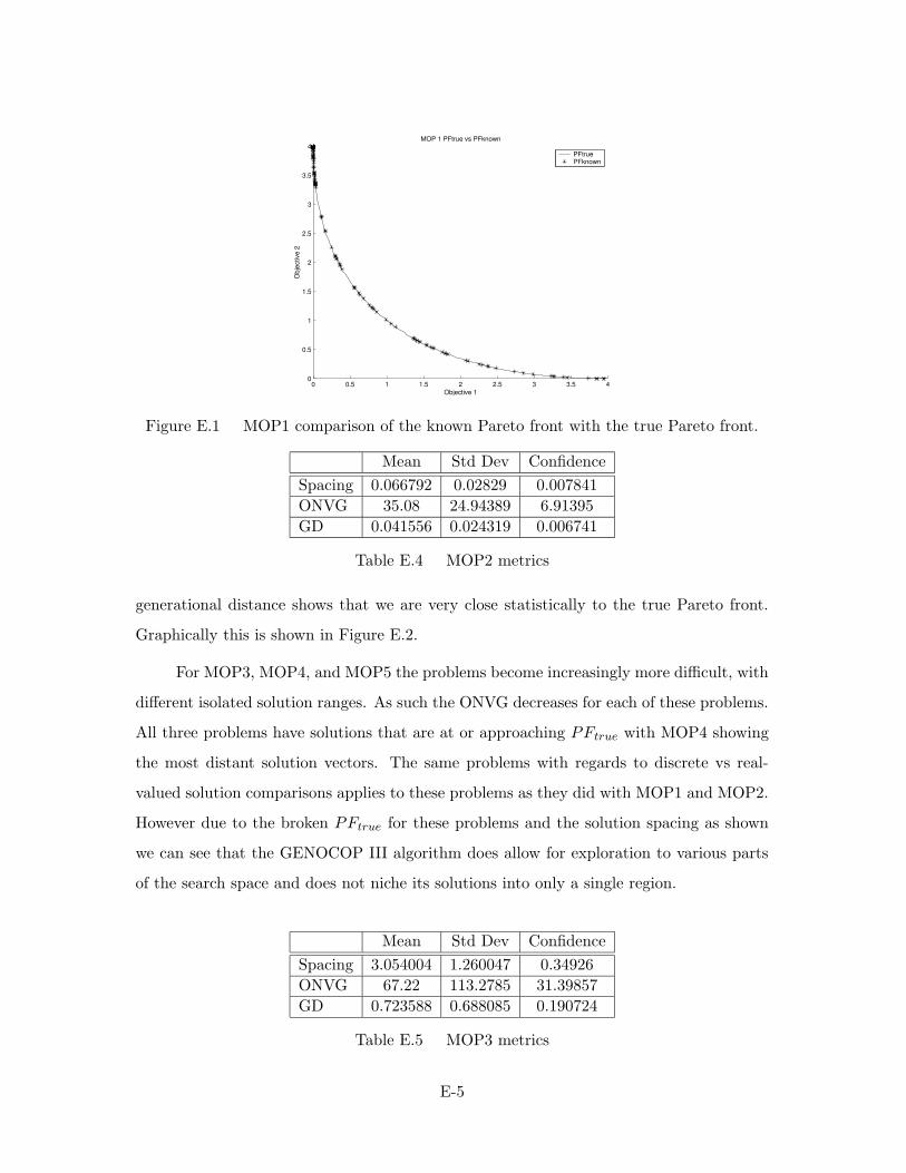
0 0.5 1 1.5 2 2.5 3 3.5 40
0.5
1
1.5
2
2.5
3
3.5
4MOP 1 PFtrue vs PFknown
Obj
ectiv
e 2
Objective 1
PFtruePFknown
Figure E.1 MOP1 comparison of the known Pareto front with the true Pareto front.
Mean Std Dev Confidence
Spacing 0.066792 0.02829 0.007841
ONVG 35.08 24.94389 6.91395
GD 0.041556 0.024319 0.006741
Table E.4 MOP2 metrics
generational distance shows that we are very close statistically to the true Pareto front.
Graphically this is shown in Figure E.2.
For MOP3, MOP4, and MOP5 the problems become increasingly more difficult, with
different isolated solution ranges. As such the ONVG decreases for each of these problems.
All three problems have solutions that are at or approaching PFtrue with MOP4 showing
the most distant solution vectors. The same problems with regards to discrete vs real-
valued solution comparisons applies to these problems as they did with MOP1 and MOP2.
However due to the broken PFtrue for these problems and the solution spacing as shown
we can see that the GENOCOP III algorithm does allow for exploration to various parts
of the search space and does not niche its solutions into only a single region.
Mean Std Dev Confidence
Spacing 3.054004 1.260047 0.34926
ONVG 67.22 113.2785 31.39857
GD 0.723588 0.688085 0.190724
Table E.5 MOP3 metrics
E-5

0 0.1 0.2 0.3 0.4 0.5 0.6 0.7 0.8 0.9 10
0.1
0.2
0.3
0.4
0.5
0.6
0.7
0.8
0.9
1MOP 2 PFtrue vs PFknown
Obj
ectiv
e 2
Objective 1
PFtruePFknown
Figure E.2 MOP2 comparison of the known Pareto front with the true Pareto front.
−20 −18 −16 −14 −12 −10 −8 −6 −4 −2 0−25
−20
−15
−10
−5
0MOP 3 PFtrue vs PFknown
Obj
ectiv
e 2
Objective 1
PFtruePFknown
Figure E.3 MOP3 comparison of the known Pareto front with the true Pareto front.
Mean Std Dev Confidence
Spacing 1.259353 0.525099 0.145547
ONVG 12.02 5.164597 1.431525
GD 1.378669 0.685502 1.90008
Table E.6 MOP4 metrics
Mean Std Dev Confidence
Spacing 0.871082 0.743527 0.206091
ONVG 8.8 5.283783 1.464561
GD 1.72786 1.492503 0.143693
Table E.7 MOP6 metrics
E-6

−20 −19 −18 −17 −16 −15 −14−12
−10
−8
−6
−4
−2
0
2MOP 4 PFtrue vs PFknown
Obj
ectiv
e 2
Objective 1
PFtruePFknown
Figure E.4 MOP4 comparison of the known Pareto front with the true Pareto front.
0 0.1 0.2 0.3 0.4 0.5 0.6 0.7 0.8 0.9−0.6
−0.4
−0.2
0
0.2
0.4
0.6
0.8
1
1.2
1.4MOP 6 PFtrue vs PFknown
Obj
ectiv
e 2
Objective 1
PFtruePFknown
Figure E.5 MOP6 comparison of the known Pareto front with the true Pareto front.
E-7

Appendix F. Parallel Evolutionary Algorithm Approaches
There are a many different types of parallelized EAs. Some parallelization schemes have
single populations, others have multiple independent distributed populations. Each type
should be examined with respect to its overall benefits to different applications. The
literature has typically defined three main classes for parallelized EAs[10]:
• Global Single-Population Master-Slave
• Single-Population Fine-Grained
• Multiple-Population Coarse-Grained
An examination of each allows an understanding of the advantages and disadvantages
and permits an optimal selection for our particular distributed system.
F.1 Global Single-Population Master-Slave
A global single-population master-slave EA (also known as a micro-grain EA) uses
a single panmictic population evolved by a single master processor that sends to each
slave process the chromosomes to be evaluated [10]. Thus all of the genetic operators
are controlled by the master process and the other processors are only responsible for the
evaluation of the different potential solutions.
The primary advantage to this type of approach is that it is basically equivalent to a
serial EA, with only the evaluations ported to outside processors. This makes it a relatively
easy matter to distribute the EA. However, it’s being equivalent to a serial approach does
prevent it from helping to be effective against premature convergence. With regards to the
parallel communication each processor must communicate solely to the master processor.
This creates a bottleneck to the system in that this approach is heavily dependent on the
communication ability of the master process.
F.2 Single-Population Fine-Grained
A fine-grained EA also has a single massive population. This time though, as opposed
to the master-slave approach, the entire population is distributed across the processors.
F-1

The processors then are allowed to communicate with other processors only within prede-
fined neighborhood regions. Thus selection and genetic operators are constrained such that
they only work on population members within each specific neighborhood. This approach
does allow for some genetic diversity in that the neighborhoods are allowed to overlap
between each other.
Because of the manner which the neighborhoods interact each neighborhood is al-
lowed to explore its own region of the search space. The communication via the overlap-
ping areas of the neighborhood allows for genetic diversity amongst the different popula-
tion members. Since only the outer regions of each neighborhood can communicate with
other neighborhoods genetic information is slowed from being passed to all members of
the population. This effectively reduces the chances of global premature convergence [69].
The amount of connections between each neighborhood thus is extremely important. If
the neighborhoods are too highly connected the genetic flow is too fast, if they are too
sparsely connected then the flow is too slow.
F.3 Multiple-Population Coarse-Grained
A multiple-population EA (also known as a multiple-deme EA) consist of a single
master processor that controls the execution of several subpopulations across the slave pro-
cessors. Typically this is designed such that each slave process has a single subpopulation.
As opposed to the grey area for overlapping neighborhoods of the fine-grained model, the
coarse-grained approach has each subpopulation as being distinct and autonomous. Thus,
migration between different populations must be explicitly handled for this approach. This
model of parallelization is similar to the island model of distributed algorithms.
Because of the infrequent communication between unique populations this type of
parallelization allows for an increased coverage of the search space. With a single popula-
tion EA’s tend to converge whereby the generated chromosomes do not have much change
from their parents. With the different populations the algorithm can explore different re-
gions of the search space each with a sporadic genetic injection occurring when members
of the surrounding populations transfer some of their solutions to their neighbors, thus
increasing the diversity of each population.
F-2
From a parallel point of view this approach does not have the communication bot-
tleneck that the micro-grain EA has. It also allows for single point to point contact, as
opposed to the communication within neighborhoods that the fine-grain approach does.
However, with this benefit comes more options on how to migrate between the subpopu-
lations.
Another method of parallelization is to use synchronous island migration. With this
type of policy each of the subpopulations evolves to a point and then they all transfer at
the same time. This only works for populations that are ensured to evolve simultaneously.
One way around this problem is to make the EA asynchronous. With an asynchronous
model each subpopulation transfers genetic material only when they individually deem it
worthwhile. Unfortunately this too has a disadvantage in that with this approach typically
only the high fitness members are distributed. This is not a problem until you realize
that the high fitness chromosomes are typically too different from the already developed
subpopulation that they were sent to that they do not help move the search [69].
F.4 Complexity Analysis
The algorithmic complexity of an evolutionary algorithm is equal to the amount of
evaluations that must be performed by the algorithm. Thus if we set tmax as the maximum
amount of evaluations that the algorithm must perform we would have a complexity of
O(tmax). As long as this number is relatively low this algorithm is efficient. As we increase
this number the effectiveness increases, but the efficiency decreases. The only good thing
is that the efficiency decreases linearly. Thus even with a large amount of evaluations we
still have an algorithm that is relatively faster than some of the deterministic approaches.
For a general evolutionary algorithm the serial time to complete the execution is
proportional to the amount of executions the algorithm is to perform Ts ≈ k · tmax. When
comparing it to a coarse grain parallelized version we assume as a worst case that each
individually parallelized EA executes the same tmax evaluations. Thus our parallel runtime
would be as given in Equation F.1. The first item on the right hand side represents the work
actually done by the individual EA’s, the second represents the startup time required to set
up each processor for the EA’s, and the third represents the time necessary to communicate
F-3

the good chromosomes between the different populations (assuming it is done only once
per generation of the children). Asymptotically this is O(tmax).
Tp = tmax + p · ts + tw ·tmaxλ
(F.1)
An examination of the speedup as shown in Equation F.2 shows that we, as expected,
do not gain any speedup from parallelizing in the coarse grain manner. Even though we
do not gain any speedup we must remember that by parallelizing the EA we are allowing
for a fuller examination of the search space, thus generating a more effective solution set.
Our efficiency of the algorithm thus is 1/p showing that our implementation is not cost
optimal.
S =tmaxtmax
= 1 (F.2)
F-4

Appendix G. Parallel Implementation
In GENOCOP III implementation each execution of the meta algorithm generates a text
file containing the parameters for executing the sublevel algorithm. When the modified
GENOCOP III(MOGENO) system is started, the algorithm must ensure that each pro-
cessor receives its own unique file so that no two processors compete for file resources.
This arrangement is beneficial to the coding in that minimal information must be directly
sent from the control processor to the slave processors. Its primary disadvantage is the
communication time necessary for file I/O for each file in the system.
Unfortunately we cannot escape this problem. The way that the overall system has
been built each of the EA’s are themselves independent of the others. Thus when the
allocation EA is run, it does so as if there doesn’t exist any meta-level EA. By doing
this we create transparency for the overall system. This also allows us, to incorporate this
algorithm into a GUI front end so that it can be used by a distributed system administrator
for allocating processes, without having to deal with the meta algorithm.
Load balancing of this algorithm occurs automatically. Each of the meta-algorithms
are executed with the same basic parameters, changing only the random seed so that
they can explore different regions. Thus every processor has it’s own full version of the
MOGENO algorithm executing on it. The only processor that does not participate in this
is the master processor, which is used for bookkeeping and control of the slave processes.
Synchronization of the different slave processors occurs via the master processor
at the beginning and end of the execution. Once the master processor has set up and
transmitted all of the necessary data structures to the different slaves then each of the
slaves are allowed to begin. Synchronization at this point is crucial in that the slaves
cannot be allowed to begin execution until after the master processor has generated the
necessary files that each processor requires for execution. During execution, since each of
the processors are running their own unique version of the EA synchronized communication
is not viable. For transmission of migrating chromosomes an asynchronous nonblocking
transmission occurs, such that once a new chromosome enters the system it is allowed to
enter the population.
G-1

The migration policy is based off of a logical ring, such that each population transmits
a single Pareto non-dominated member, randomly selected from the Pareto known set.
This selection occurs at the end of each reference population generation. The selected
individual is then transmitted to the populations ranked one higher and one lower on the
logical ring.
For this algorithm the only communication that is necessary is from each processor
to the processor ranked higher and lower than it. In this manner we hope to allow a slow
migration of members between the populations. Of course we have wrapping whereby
those processors that are ranked first and last (not including the master process) transfer
to each other as well as their standard neighbors.
G.1 Implementation Protocol
This implementation is done using MPI commands. We use both blocking and non-
blocking communication protocols to transfer the data. Every send command is done using
a blocking command so that the information could be sent prior to it being modified. We
use non-blocking receive commands in order to pull the data when migrating so that we
don’t’t have to make all of the processors wait for algorithm to finish.
In comparison with some of the other protocols available for use in this implementa-
tion (mainly Java RMI, and C sockets) we decided that MPI is the most suitable. First of
all this program is written in C, thus a Java interface would add unnecessary complexity
to the implementation. Beyond this, if we use RMI we would have to set up the pro-
gram such that the EA itself is a remote method. We would then have to call the remote
method from some control system. That would allow us to have the program distributed.
As for communication between the different EA populations (migration) we would have
to implement a separate communication structure (another RMI interface, or more likely
direct sockets) that would communicate between the different EAs running. Overall this
approach would be unnecessarily complicated because of all of the overhead control that
would need to be implemented so that each RMI instantiation of the program would know
how to communicate with it’s neighbors.
G-2

Sockets, being that they use the same fundamental layer as RMI, are not much better.
If we used a socket implementation for this program then we would have to have a very
specific, and potentially static, amount of processors. We would then have to set up each
processor individually so that it could be the client/server as needed. This would involve a
lot of overhead time for no relative improvement. This approach also has the downside of
the intra-processor communication in that we would have to specifically encode into each
separate EA instantiation what processors it must communicate with in order to migrate
individuals.
That leaves us with using MPI for this project. MPI is implemented in C and thus
can be incorporated directly into our algorithm. It has the advantages that we do not need
to set up each individual implementation for every processor. Instead we create our single
executable and it ports itself to the different processors. It then executes on the different
processors as coded.
With MPI we also have an efficient way of identifying processors as being neighbors.
MPI uses a built in ranking system, thus for our implementation we can consider each
processors neighbors as being the processors with a rank one higher or one lower. Since
we know the rank of these processors we can simply communicate to them using the built
in MPI calls. With this approach MPI makes HPC programming much simpler than some
of the alternative methods.
G.2 Scaleability
Since the GENOCOP III system has a worst case serial performance of O(t2max), we
can set that as our serial time for a single execution, thus ts = t2max. We can use the number
of evaluations as our measure of the time of the system since it’s amount determines the
actual runtime of the system. When we are considering a parallel execution we have a
serial time of p times the serial time of a single execution, because for our implementation
we run p individual executions when executing in parallel. For calculating the parallel run-
time (tp) we must consider not only the time to do work(W ) but also the time necessary
for the startup of the system, and the time necessary to communicate individuals between
the different populations.
G-3

The time necessary to do the work on the parallelized version of the EA is no different
from the serial one, except that it is now distributed, thus while a comparable serial version
takes p(t2max), we can do the same amount of work in parallel with only p(t2max)p = t2max.
The startup time for this system involves the initial setup of the different EA’s. Since
there are p − 1 EA’s to be set up our setup time is ts(p). Finally, the time to transfer
information between the different system is based on a transfer of a single Pareto non-
dominated chromosome once every time through the reference population. Since we have
a maximum of tmax evolutions of the reference population the total communication would
be tw(tmax). Thus our total parallel runtime can be expressed as Equation G.1. Thus the
time complexity for this parallel algorithm is O(t2max) and thus cost optimal.
Tp = t2max + p · ts + tw · (tmax) (G.1)
With this equation we can calculate the exact speedup of the parallelized version.
Speedup is defined as the ratio of serial time to parallel time or Ts
Tp. Since the time order
complexity of the serial implementation is O(p(t2max)) and the parallel implementation is
only O(t2max) our speedup is then given by Equation G.2.
S =p(t2max)
t2max= p (G.2)
With this speedup we can calculate the efficiency. Efficiency is given as the ratio of
the speedup over the number of processors executing the algorithm. With p processors
executing and a speedup of p we have an efficiency of O(1). Thus by definition we have a
cost optimal system.
Finally we get to the isoefficiency function. The isoefficiency function determines
the actual scalability of the system. If we let K = E/(1 − E) then the isoefficiency can
be calculated as W = KTo(W,p) where To(W,p) represents the overhead time given as a
function of the work (W ) and the amount of processors (p). To(W,p) can be calculated as
the amount of time that is not directly affected by work or pTp −W . Thus for our system
G-4

since we have a work of W = p(t2max) the overhead time is given as
To = (p(t2max) + p2 · ts + p · tw · (tmax))− p(t2max) (G.3)
To = p(p · ts + tw · (tmax) (G.4)
We then examine each of the remaining terms individually. First examining the term
based on the system startup we have W = Kp2ts. For the communication time we have
W = p(t2max) = Kptwtmax, eliminating the right hand side tmax term we haveW = K2ptw.
Thus between the two function the overall asymptotic isoefficiency is asymptotically equal
to O(p2). This is clearly not a linear isoefficiency, thus showing that the system is poorly
scalable.
The only problem with the above calculations is that they are not fully telling about
the reality of the system. In actuality we do not yet have a full understanding of what
percentage of tmax the parallel system requires to execute so that it would provide results
comparable to the tmax evaluations of the serial algorithm. Currently for these experiments
we do not run (p − 1)tmax evaluations of the serial algorithm. We do run that lessened
amount of evaluations of the parallel algorithm, simply because we have no knowledge of
what percentage of the serial algorithm each subpopulation needs to run. Doing the same
metrics based on the idea that the serial run is only run one time, as opposed to p, we
have the same Tp, but our speedup becomes equal to 1, making our efficiency equal to 1/p.
Our isoefficiency remains at O(p2).
This shows that evolutionary algorithms are non-scalable algorithms. Whereas you
can add as many EAs to a system as you would like, as long as you keep the number of
evaluations constant you do not gain any performance improvement. On the other hand,
research efforts have shown that by parallelizing the algorithm it is possible to decrease
the amount of evaluations per population and find improved results over a serial EA. It is
this ratio of how many populations to evaluation size that needs further examination with
respect to the EA community.
G-5

EA’s cannot in themselves be parallelized too easily. Typically the only item that
can be parallelized is the evaluation function, this is the basis for the master-slave model.
The problem with this parallelization is that the communication overhead necessary for
transferring that function out and returning the result can be overly costly for the overall
system. Thus, as shown in the diffusion and island models, typically the whole EA is sent
out for execution on individual processors.
Unfortunately, once you send the entire EA algorithm out, you lose any speedup
that would be gained by parallelizing the algorithm. Only by decreasing the number of
evaluations that the system has can we manage to decrease the overall execution time. As
has been shown in many previous papers [11] [9] a better solution can be found with a
smaller amount of evaluations per EA using a parallel system. Finding this ratio between
the amount of populations and the evaluations amount is therefore vital for increasing the
efficiency of parallel EA systems.
G.3 Parallel Meta Experimentation
Experimentation of the parallel meta-EA requires analysis of communication struc-
tures, processors differences, I/O structures, scalability. For all of this research investiga-
tion we use standard statistical analysis equations of mean, median, max, min, variance,
and standard deviation. We also use statistical T-tests in order to compare the means of
different results using the standard principles of statistical hypothesis testing[53]. While
we primarily examine the execution times of these results we also do examine the multi-
objective metrics of spacing and ONVG for as described in Section E.1.
I/O Impact In order for the allocation EA to be quickly deployed to a real world
environment the inputs concerning the hardware comparisons as well as the current sys-
tem state information and change request are all external inputs that are read in by the
Allocation EA during execution. For this reason there is a lot of disk I/O that is required
by each execution of the allocation EA algorithm. Since the meta-EA executes multiple
allocation EA’s for the parameter optimization a large amount of file I/O is required.
G-6

The initial parallelization of the meta-EA used a shared disk access such that all
processors were competing with each other for read/write privileges across the network
and on a single drive. This created a deadlock situation that slowed the processors ability
to do the work needed. By trying to access the shared drive the processors also had to wait
for the delay caused by having to have the file data communicated across the network.
In order to solve this problem the processors were made to use the local hard drive.
This removed any deadlock due to waiting for other processors, it also removed any network
latency that is delaying the processors computations. As shown in the following hypothesis,
this experiment is based on statistically testing the average time (t) used by the meta-EA
to calculate a solution set using shared and local I/O constructs. For this experiment we
use the parameters as given in Table 6.3 and run each experiment 5 times on a simple 16
processor, 4 process experiment.
Hypothesis 5 The time necessary to do a complete run of the meta-EA is less using local
file I/O then using shared file I/O.
H0 : µt(shared[1])..t(shared[m]) = µt(local[1])..t(local[m])
H1 : µt(shared[1])..t(shared[m]) > µt(local[1])..t(local[m])
Communication Impact To test the communication impact on the parallelized meta-
EA we run the algorithm on four processors across both the fast-ethernet and Myrinet
backplanes. The processors for this experiment are all 1.0GHz Intel Pentium 4s so as to
provide the same computational capacity for each backplane type. The experiments are
run 5 times each using the parameters as given in Table 6.3 for a 16 processor, 4 process
system. Given that there is very limited communication necessary during the execution the
hypothesis is that there is not a statistically different time difference between the different
backplane experiments as shown:
Hypothesis 6 There is not a statistically significant difference between the fast-ethernet
and the backplane experimental times of the meta-EA.
H0 : µt(Fast−Ethernet[1])..t(Fast−Ethernet[m]) = µt(Myrinet[1])..t(Myrinet[m])
H1 : µt(Fast−Ethernet[1])..t(Fast−Ethernet[m]) 6= µt(Myrinet[1])..t(Myrinet[m])
G-7

Processor Impact To test the processor impact on the parallelized meta-EA we run the
algorithm on four processors each on a AMD Athlon 1.7 GHz system and a Intel Pentium
4 1.0GHz system using a Fast-Ethernet backplane on both systems. The experiment is
run 5 times each using the parameters as given in Table 6.3 for a 16 processor, 4 process
system. Since the AMD is a faster chipset with a faster math processor it is expected to
have a faster overall time for execution.
Hypothesis 7 There is not a statistically significant difference between the fast-ethernet
and the backplane experimental times of the meta-EA.
H0 : µt(Athlon[1])..t(Athlon[m]) = µt(Pentium[1])..t(Pentium[m])
H1 : µt(Athlon[1])..t(Athlon[m]) > µt(Pentium[1])..t(Pentium[m])
Scalability Performance In order to examine how well this algorithm scales based on
number of processors, experiments are done using the parameters as given in Table 6.3 for
each of the systems as depicted in Table 6.1. These are run 5 times each and are examined
with respect to execution time, ONVG, Pareto dominance, and spacing. A comparison
between the different groups is also done to gain some understanding on how the program
scales with respect to the problem size.
For this experiment it is expected that the executions with the larger amounts of
processors has a better spacing with a larger ONVG and potentially more dominating
set of solutions. This is due to the fact that with the higher number of processors we
are effectively increasing the overall population size. This increases the amount of search
space that can be covered, allowing for better solutions. The overall runtime for these
experiments is expected to not be significantly different as they are still each running the
same basic EA on each processor.
Hypothesis 8 There is not a statistically significant difference between the experiment
running on few processors compared to one running on a large amount of processors with
the meta-EA.
H0 : µt(small[1])..t(small[m]) = µt(large[1])..t(large[m])
H1 : µt(small[1])..t(small[m]) 6= µt(large[1])..t(large[m])
G-8

G.4 Parallelizability Analysis
I/O Results
Mean Time Std Dev
Shared 294840 n/aLocal 12913 513
Table G.1 The mean time differences for the meta-EA executed on shared and local filesystems.
The initial experiments with the meta-EA consisted of using the shared directory for
file storage. This created a bottleneck between processors attempting to read/write to files
as well as communications trying to access the directory. In order to alleviate this problem
the files were transferred to local directories so that each processor had control over it’s
own data set. This removed any problems occuring based on file read/write bottlenecks
as well as alleviating the problem of communication to the shared directory.
Another problems with having to transfer file data across the network is that the
algorithm is being subjected to the whims of the network load. At any given time the
network traffic could overwhelm the network and all of the processors would have to wait
until there is sufficient bandwidth to communicate with the file storage area. Since some of
the files are kept open throughout the execution of the algorithm, the overhead necessary
to maintain these ever growing files could in themselves overwhelm the communication
links. This in effect would cause a denial of service by the program itself.
As shown in Table G.1 the mean time for running the algorithm using the shared
directory is roughly 22.2 times as much as running the algorithm locally. Because of this
large time difference the parallel execution is not executed more than once.
Communication Results
Spacing ONVG Time
Communications 0.536193242 0.206151006 0.60971799Processors 0.002530942 0.003834864 0.005711524
Table G.2 Student T-test probabilities based on comparison of Myrinet and Fast-Ethernet (two-tailed test) as well as Intel vs Athlon Processors (one-tailedtest)
G-9

Figure G.1 ONVG comparison for three platforms. The error bars represent variance.
Figure G.2 Spacing comparison for three platforms. The error bars represent standarddeviation.
Using a standard student T-test to calculate the P-values for comparing the samples
from the different communication backplanes we get results as shown in Table G.2. Since
all of the values are well above our alpha of 0.05 we must fail to reject H0 and thus conclude
that the all of the metrics are statistically equivalent. Thus there is no statistical difference
for running this algorithm using different backplanes, assuming everything else being equal.
These results are also shown in Figures G.2, G.1, G.3
Processor Results
When comparing the processors all of the P-values are less than our alpha of 0.05.
Thus we must reject H0 and conclude that the mean difference for all of our metrics are
statistically different between processors. For the first metric, that of spacing, we must
conclude that AMD Athlon system has the greater spacing. For the ONVG we must
conclude that the Pentium system has the greater ONVG. Finally for the metric of time
we must conclude that the Athlon has the higher time and thus is slower. Thus in all areas
G-10
s e 7 e
i ^ O 4
3 2 1
Msta EA ONVG on 16 Procsssor, 4 Procsss Expsriment
T , * . —m
-
1.0 SHJ ln1»IP»n1iumlll, 1 OGhz AMP ttlhlcn, F*! 1 Dfihz Inlel Penlium l||,
Fist Ethirnit Ethirnit hjtvnntt
Msta E A Spacing on 16 Processor, 4 Process EKpsrImsnt
20XIX
2CIXIX
f lOXCO
^^ 1.0 OHi Intil Ptntlum 1.40hi AMD Athlon, 1 OGr.z initi P^rrtiur
III, Put Ethirnit Put Ethirnit rgtvnnit

Figure G.3 Time comparison for three platforms. The error bars represent standarddeviation.
the Intel Pentium system has the advantage. This is not the expected result, and may
be due to the large amount of file I/O required by the meta-EA. The Intel chips have in
the past shown improvement over the AMD chips for dealing with file I/O problems. This
could be the case for these experiments as well.
Scalability Results
Figure G.4 Time comparison for different numbers of processors on Fast Ethernet, IntelPentium 1.0Ghz Systems running on a 16 processor 4 process experiment.The error bars represent standard deviation.
The statistical results for the scalability of the 16 processor, 4 process experiments is
given in Table G.3. For this experiment we can see that the spacing between the problems
executed with 4 processors and the 8 processors are statistically equivalent. As shown by
Figure G.6, the variance of the experiment executed with 4 processors overlaps that of the
experiment done using 8. The experiment run on two processors is statistically greater
than the other two processor sizes, thus meaning that we are producing a better spacing
G-11
Msta EA Tims DIITsrGnce on 16 Procsssor, 4 Procsss EKpsrImsnt
145D0 14X0
2 13X0 I 13X0 P 12X0
12X0 11X0 11X0 :^ ^
1.0 OHz Intil Pintlum III, FiitEthirnit
1 OGlu AMP Athlon, Fist Ethirnit
I.OOhzlnWPwVum*, hjtvrlnit
Meta EA Time DifTerence on 16 Processor 4 Process Experiment
T 15X0
1" i
^ ICCOO
p
0
2 4 s Number of Procesors

Figure G.5 ONVG comparison for different numbers of processors on Fast Ethernet, IntelPentium 1.0Ghz Systems running on a 16 processor 4 process experiment.The error bars represent standard deviation.
Figure G.6 Spacing comparison for different numbers of processors on Fast Ethernet, In-tel Pentium 1.0Ghz Systems running on a 16 processor 4 process experiment.The error bars represent standard deviation.
for the Pareto front when using the larger amounts of processors. This result is expected
as the larger processor amount relates directly to a larger amount of populations being
executed in parallel. Thus there are more chances of finding more regions of the Pareto
front.
When examining the ONVG for this problem the large variance by the execution
using 8 processors overlaps both with the 2 processor and 4 processor experiments (see
Figure G.5). Thus the ONVG for the 8 processor experiment is statistically equivalent
to these two experiments, as shown by Table G.3. However, the ONVG for the 2 and 4
processor experiments are not statistically equivalent to each other as there is no overlap
in variance.
G-12
Msta EA ONVG on 16 Procsssor, 4 Procsss Expsriment
10 s e 7
0 e 1 6 O 4
3 2 1 0
m Numbir of Prooisors
50X11X1
5IX0C0
20XIX
2IXCIXI
lOXCO
UXOCO
SDOi
0
Mela E A Spacing on 16 Processor, 4 Process EKpsrimsnt
m Numbtr of Proasorr

Spacing ONVG Time
2 vs 4 0.002182753 0.006790647 0.1308723082 vs 8 0.001017604 0.343376341 0.0757212494 vs 8 0.064575207 0.585314338 0.027376783
Table G.3 Student T-test probabilities based on comparison of different processor sizesusing a two-tailed test with an alpha of 0.05 and a 16 processor 4 processproblem.
The statistics concerning the time necessary for the different processor amounts shows
that the 2 processor experiment is statistically equal to both the 4 and 8 processor exper-
iments. As Figure G.4 displays the time necessary for the two processor experiment is in
the middle of the time necessary for the 4 processor and 8 processor experiments, with the
4 processor one being statistically lower (and thus faster) than the 8 processor experiment.
Figure G.7 Time comparison for different numbers of processors on Fast Ethernet, IntelPentium 1.0Ghz Systems running on a 64 processor 16 process experiment.The error bars represent standard deviation.
Spacing ONVG Time
2 vs 4 0.004110467 0.000991679 0.0009234672 vs 8 0.000405308 0.002895812 8.8629E-094 vs 8 0.000411025 0.009987842 0.288112704
Table G.4 Student T-test probabilities based on comparison of different processor sizesusing a two-tailed test with an alpha of 0.05 and a 64 processor 16 processproblem.
Table G.4 shows that the only statistic that is equal for the 64 processor 16 process
problem is that of time between the 4 processor and 8 processor experiments. As shown in
Figure G.7 for this experiment it again took longer to execute the 2 processor experiment
than either of the experiments using 4 or 8. As for the ONVG Figure G.8 shows that the
G-13
Meta EA Time DifTerence on 64 Processor, 16 Process Experiment
* ^CCOD
'- 20X0
ICCOO
m
2 4 S
Number of Procesors

Figure G.8 ONVG comparison for different numbers of processors on Fast Ethernet, IntelPentium 1.0Ghz Systems running on a 64 processor 16 process experiment.The error bars represent standard deviation.
Figure G.9 Spacing comparison for different numbers of processors on Fast Ethernet,Intel Pentium 1.0Ghz Systems running on a 64 processor 16 process experi-ment. The error bars represent standard deviation.
4 processor experiment had the highest overall, followed by the experiment running 8 and
lastly that running on 2. As shown in Figure 7.3 the Pareto front for the larger amount of
processors dominates that found by the smaller amount, thus the smaller ONVG can be
attributed to a converging solution set. This is further shown by the decreasing spacing as
the processors increase (see Figure G.9), these are also statistically not equal.
For the experiment using a 128 processor 16 process problem we find that none of the
processor amount on any of the metrics are statistically equivalent (Table G.5). As shown
in Figure G.11 our ONVG increases as the processors increase, showing we are finding
more members of the Pareto front. In contrast to the 64 processor, 16 process experiment
our time also increases with amount of processors executing as given in Figure G.10.
G-14
MetaEAONVG on e4Processorp 16 Process EKperlment
2 4
Numbir of Prooisors
ecxoco
TCCOCO sccoco
g uxoco
^ 3CC0C0
2CIXIX
ICCOCO
0
UetaEA Spacing on 64 Processor, 16 Process EKperiment
T ^^^
I VIH ^ 1
2 d 8
Numbtr of Proasorr

Figure G.10 Time comparison for different numbers of processors on Fast Ethernet, IntelPentium 1.0Ghz Systems running on a 128 processor 16 process experiment.The error bars represent standard deviation.
Figure G.11 ONVG comparison for different numbers of processors on Fast Ethernet,Intel Pentium 1.0Ghz Systems running on a 128 processor 16 process ex-periment. The error bars represent standard deviation.
The spacing however is highest with the four processor experiment, and the 8 processor
experiment has a spacing just below that (Figure G.12).
The overall parallel scalability results show us that, in general, the solutions improve
as the number of processors increase. This is as expected since by increasing the number
of processors we are effectively simply increasing the number of populations. These pop-
ulations however do interact via migrations. The migration allows for the populations to
search a greater amount of the search space and thus find more dominant solution vectors.
With these more dominant solution vectors the Pareto front changes size. Because
the more dominant solutions pushes the Pareto front towards a smaller region of the
search space the solutions can have a large variety of different results for ONVG and
spacing. Typically we would expect a higher ONVG to occur as the number of processors
G-15
Meta EA Time D ilference on 128 Processor, 16 Procoss ExperiiiienI
I^HAHU , , IQCOCO
-,2roco
£ ecoco •- QCOCO
'i 2C0C0
14 5
Numb*r rn Proc*»ors
Meta EA ONVG on 128 Processor, 16 Process Experiment
12
in
s G i B o
4
1
^^^^ 2
0 2 4 S
Hjmber of Procesors

Figure G.12 Spacing comparison for different amount of processors on Fast Ethernet,Intel Pentium 1.0Ghz Systems running on a 128 processor 16 process ex-periment. The error bars represent standard deviation.
Spacing ONVG Time
2 vs 4 0.000386934 0.000982802 0.002929962 vs 8 n/a n/a 2.33971E-074 vs 8 0.041403522 0.001608867 0.017735258
Table G.5 Student T-Test probabilities based on comparison of different processor sizesusing a two-tailed test with an alpha of 0.05 and a 128 processor 16 processproblem.
increase since we expect to find more solutions. However when we move to the more
dominant solutions we can very quickly remove old non-dominated solutions that have
become dominated, this decreases our ONVG yet the solutions are more dominant.
The same effect occurs to the spacing, however this metric can vary more readily.
When the overall dominance increases of the solutions set the solutions end up moving to
a smaller region. This pushes the solutions closer together thereby reducing their spacing.
Thus even with a lower ONVG we can still produce a lower spacing simply because the
Pareto front encompasses a smaller region of the search space with the more dominant
solutions.
As for the time required for each experiment, since the algorithm is a stochastic search
we cannot predict the exact runtime for any execution. The chromosomes generated might
require a great deal of time to execute or the might require a very small amount simply
on by the random selection of the chromosomes values. With this said we can make a
generalized statement that the chances for an extra long or extra short execution would
G-16
6CC0C0
4CC0C0
^2CiXiX
idxco
0
^eta EA Spacing on 12B Processor, 16 Process EKperlment
^^ ^ 1 1
2 4 S
Numbtr of Proa sort

occur for the larger amount of processor executions. Thus the executions using the 8
processors is expected to, on average, have the greater variance for runtime.
Solution Generation
0.2 0.3 0.4 0.5 0.6 0.7 0.8 0.9 1 1.1 1.20
0.2
0.4
0.6
0.8
1
1.2
1.4
1.6
1.8
2x 10⁶ PFront Comparison on 4 Processors
Num
ber I
tera
tions
(Obj
1)
Effectiveness (Obj 2)
Processor 1Processor 2Processor 3Processor 4
Figure G.13 Comparison of the individual processor Pareto fronts running a 16 processor4 process experiment on four processors.
Another aspect that is examined is how the multiobjective parallelism works in terms
of generating an overall solution. Since there is only a limited amount of communication
between processors, and only at the conclusion of each generation the overall system does
not converge overly quickly. Each processor acts independently of the other processors and
thus is allowed to cover a different region of the Pareto front than the other processors.
This is shown in Figure G.13 whereby each processor covers a slightly different region of
the Pareto front, yet overlap among the processors does exist.
G-17

Appendix H. Meta-EA Parameter Results
The parameters optimized by the meta-EA can be divided into three categories based on
their sizes. The first category, as shown in Figure H.1, contains those elements that are
greater than 100. The second category includes those elements that are boolean values
as shown in Figure H.2. The final category includes the operator frequencies as shown in
Figure H.3.
When examining these charts it is important to note that they are representing
the mean Pareto solution found. This point may or may not be feasible with respect to
providing an effective execution of the allocation EA. These graphs are more figures to
illustrate the comparative results that the different sized problems generated. The error
bars in these graphs represent the confidence interval based on the sample data. The full
statistical results of each of the different sized experiments are provided at the end of the
chapter. Overall the mean Pareto results appear to be statistically equivalent across the
different problem sizes.
Figure H.1 Parameter comparison for the large meta generated parameters.
In the large scale parameters chart (Figure H.1) the most noticeable trend is that
the reference population size is just slightly smaller than the search population size. This
is most likely due to the fact that the reference population is a background population
H-1
Pai3meterComna"isonrorLarc|eScJePararTie(efs.MeTaEfl
3SXi
Rdpiewe S««h PopiMilion Nufnbtrof HAienc* Nunhr Of Ok ping Popd J»n £d* Sbi EdlidiDfd PopuUPon Enhiioft br fttL Pop.
Ptnod
Phsm^et
10 Proowod. 4Procn^«& mG^FiiycttuHt. laProocuci Dl28Proo»0B, 10 Proc«^^«s
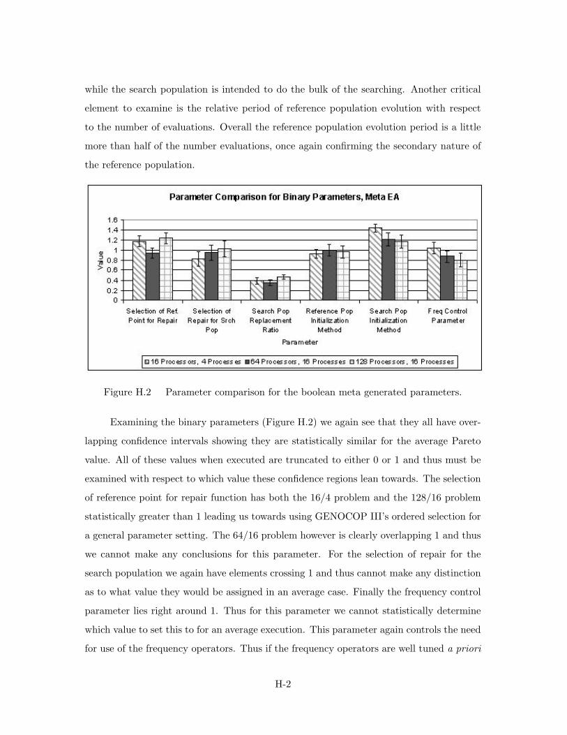
while the search population is intended to do the bulk of the searching. Another critical
element to examine is the relative period of reference population evolution with respect
to the number of evaluations. Overall the reference population evolution period is a little
more than half of the number evaluations, once again confirming the secondary nature of
the reference population.
Figure H.2 Parameter comparison for the boolean meta generated parameters.
Examining the binary parameters (Figure H.2) we again see that they all have over-
lapping confidence intervals showing they are statistically similar for the average Pareto
value. All of these values when executed are truncated to either 0 or 1 and thus must be
examined with respect to which value these confidence regions lean towards. The selection
of reference point for repair function has both the 16/4 problem and the 128/16 problem
statistically greater than 1 leading us towards using GENOCOP III’s ordered selection for
a general parameter setting. The 64/16 problem however is clearly overlapping 1 and thus
we cannot make any conclusions for this parameter. For the selection of repair for the
search population we again have elements crossing 1 and thus cannot make any distinction
as to what value they would be assigned in an average case. Finally the frequency control
parameter lies right around 1. Thus for this parameter we cannot statistically determine
which value to set this to for an average execution. This parameter again controls the need
for use of the frequency operators. Thus if the frequency operators are well tuned a priori
H-2
PararreTer Corrfianson Tof Binary Paarneters.MetaEA
StlKboft of fttt StlKlHft of Stjreh Pop RriHtnc* Pop Stireh Pop Point tH fttpjir RtpJirtH Sroh ftopUcofnorri hlUliADn inliJfzAoft
Pop RAD MdhOd MdtHd
Pinm«l*r
FrtqCorriiol PdrjiTHlor
laiaProGOHOd. 4ProGac(ac MProoMion. ifi Proocuci DlSSProoMiod. ifi Proocu^

to the Allocation EA execution there would be no need to use GENOCOP III’s frequency
distribution control mode.
Figure H.3 Parameter comparison for meta generated operator frequencies.
When examining the operator frequencies it is most important to note which param-
eters are used more than others. Examination of Figure H.3 shows that operators 3,4,5,6,8,
and 10 all have clearly overlapping confidence regions. The other operators have at least
one problem size that did not have overlapping confidence regions and thus we cannot
conclude that on average the mean operator frequencies are the same for these problem
sizes.
H-3
Parametef Compvlson 'or Operafors. M«<a EA
1ft . 1
o 10
0
* Jj. Trii 1 1 'II - T , rU, n: , 1 1 rfi T ,T 1 J, XT
\ I 1 1 1 1 1 1 1 1 Optr.
1 d« Op«it« 1
2 3p«it« Op«il« Op«doi Op«J« 4
3 4 6a
p
3p*rAr Optrdor OpuiMtn OpuiMtH 7 a 0 10
BlBPiDGMioK. 4ProGM(*( BOq ProGCHOd. laProcauac ai2S Pro«H04. laProcaiiac |

Parameter 16x4 Mean Std Dev CI
Reference Population Size 389.5571987 236.2830866 57.88820677Search Population Size 505.1765954 263.0779538 64.45281889Number of Evaluations 1794.601749 928.6608601 227.517393Reference Population Evolution Period 1086.310723 507.0554062 124.2261078Number of Offspring for Ref. Pop. 145.527787 148.273022 36.3261691Selection of Ref. Point for Repair 1.172122219 0.406705698 0.099640918Selection of Repair for Srch Pop 0.822377266 0.591484159 0.144910742Search Pop Replacement Ratio 0.390549578 0.223985202 0.054875285Reference Pop Initialization Method 0.918721188 0.50532305 0.123801689Search Pop Initialization Method 1.431812313 0.526420307 0.128970414Freq Control Parameter 1.042669516 0.480504554 0.117721278Operator 1 67.0803312 25.32745276 6.205102715Operator 2 63.17349633 31.32962754 7.675606339Operator 3 39.89091375 25.44859307 6.234781501Operator 4 50.48289656 26.64996494 6.529111766Operator 5 60.75908978 26.92922281 6.597528584Operator 6 43.9275087 24.78033928 6.071062575Operator 7 40.13147564 27.13531491 6.648020148Operator 8 45.98876914 25.65930963 6.286406035Operator 9 34.38797434 26.01208124 6.372833363Operator 10 53.30268888 26.0999032 6.394349316
Table H.1 Meta-EA results for the parameters of the allocation EA for a 16 processors4 processes system
H-4

Parameter 16x4 Max Min Median
Reference Population Size 942.445679 32.092625 325.603409Search Population Size 890.102905 97.735191 488.150421Number of Evaluations 2961.243896 41.922089 2161.337891Reference Population Evolution Period 1924.893555 104.444801 932.302521Number of Offspring for Ref. Pop. 626.132202 20 94.584648Selection of Ref. Point for Repair 1.891008 0.052244 1.22514Selection of Repair for Srch Pop 1.983171 0 0.842701Search Pop Replacement Ratio 0.916667 0.001874 0.426046Reference Pop Initialization Method 1.992726 0.009834 1.079954Search Pop Initialization Method 1.9999 0.106553 1.631495Freq Control Parameter 1.884826 0.055286 1.1660775Operator 1 98.681847 8.657294 80.109917Operator 2 100 0.058279 68.82626Operator 3 97.560654 0.718009 36.577709Operator 4 98.018188 1.096463 50.765741Operator 5 98.545494 0 70.5926055Operator 6 98.319336 0.007123 42.023636Operator 7 91.266945 0.530638 32.385033Operator 8 94.602661 0.47943 51.022148Operator 9 85.407837 1.431936 30.652715Operator 10 95.657799 5.698383 64.048286
Table H.2 Meta-EA results for the parameters of the allocation EA for a 16 processors4 processes system
H-5

Parameter 64x16 Mean Std Dev CI
Reference Population Size 378.469632 207.4256501 46.94391179Search Population Size 486.9126663 313.6551585 70.98543544Number of Evaluations 1836.856824 1059.75382 239.8401057Reference Population Evolution Period 858.2391636 520.7044231 117.8441649Number of Offspring for Ref. Pop. 258.1885503 234.3820591 53.04460034Selection of Ref. Point for Repair 0.940267067 0.468000271 0.105916329Selection of Repair for Srch Pop 0.950143213 0.630041053 0.142588882Search Pop Replacement Ratio 0.353201227 0.253317903 0.0573301Reference Pop Initialization Method 0.998187587 0.400442525 0.090626876Search Pop Initialization Method 1.21491524 0.344601163 0.077989037Freq Control Parameter 0.873429187 0.491907587 0.111326957Operator 1 52.14959524 24.8780837 5.630328584Operator 2 62.89592893 21.33113909 4.82759539Operator 3 46.88721444 21.59209139 4.88665328Operator 4 53.6321004 28.10806994 6.361328772Operator 5 51.87596003 24.87783189 5.630271594Operator 6 47.2019662 27.09726997 6.132567744Operator 7 57.15969339 26.71686296 6.046475243Operator 8 43.38214701 30.07582482 6.806664782Operator 9 55.10507256 28.70109993 6.495541428Operator 10 40.72883895 21.76934745 4.926769307
Table H.3 Meta-EA results for the parameters of the allocation EA for a 64 processors16 processes system
H-6

Parameter 64x16 Max Min Median
Reference Population Size 777.286926 65.477386 330.658173Search Population Size 967.083618 97.735191 441.995972Number of Evaluations 3000 20 2316.046631Reference Population Evolution Period 1916.818237 1 908.696594Number of Offspring for Ref. Pop. 881.245239 20 127.257942Selection of Ref. Point for Repair 1.88511 0.209489 0.986488Selection of Repair for Srch Pop 1.983171 0.176697 0.908557Search Pop Replacement Ratio 0.936162 0.001874 0.434751Reference Pop Initialization Method 1.561017 0.190346 1.039173Search Pop Initialization Method 1.753513 0.709395 1.241179Freq Control Parameter 1.918222 0.141345 0.687379Operator 1 98.681847 3.422832 49.389069Operator 2 99.491371 7.600605 67.02951Operator 3 90.26947 11.349612 46.225033Operator 4 97.59063 1.096463 61.832386Operator 5 95.755798 5.909908 46.361481Operator 6 96.332153 10.424253 43.954857Operator 7 89.719986 8.030785 69.656998Operator 8 84.376366 0 39.829182Operator 9 100 0.250459 63.127525Operator 10 94.425659 5.698383 39.847404
Table H.4 Meta-EA results for the parameters of the allocation EA for a 64 processors16 processes system
H-7

Parameter 128x 16 Mean Std Dev CI
Reference Population Size 423.6037612 257.6806745 61.24559248Search Population Size 492.7267231 224.2839 53.30784066Number of Evaluations 1431.524429 1097.843723 260.9357081Reference Population Evolution Period 1111.504688 583.3293345 138.6458288Number of Offspring for Ref. Pop. 324.0205785 267.2823349 63.52771696Selection of Ref. Point for Repair 1.236747882 0.445590788 0.105908105Selection of Repair for Srch Pop 1.023674765 0.681043376 0.161870521Search Pop Replacement Ratio 0.465002706 0.20717318 0.049240961Reference Pop Initialization Method 0.964030941 0.503030269 0.119560332Search Pop Initialization Method 1.171138647 0.552814168 0.131392978Freq Control Parameter 0.800512235 0.574952432 0.136654805Operator 1 39.35214124 27.48900254 6.533591432Operator 2 48.79633788 27.11804108 6.44542124Operator 3 49.15392776 26.83640897 6.378482865Operator 4 46.73856941 20.70864032 4.92203363Operator 5 65.81685253 24.42039257 5.80424362Operator 6 51.29089465 29.4781333 7.006368415Operator 7 49.53845429 33.73221852 8.017480211Operator 8 46.83234765 28.65741858 6.811300782Operator 9 39.28663876 25.345122 6.02403349Operator 10 49.38958835 23.09131644 5.48834855
Table H.5 Meta-EA results for the parameters of the allocation EA for a 128 processors16 processes system
H-8

Parameter 128x 16 Max Min Median
Reference Population Size 942.595093 77.409317 394.523346Search Population Size 934.710815 166.93187 519.623108Number of Evaluations 2949.694336 20 1169.803711Reference Population Evolution Period 1962.057495 82.592873 968.590088Number of Offspring for Ref. Pop. 896.248291 35.958309 311.04187Selection of Ref. Point for Repair 1.998072 0.274207 1.363202Selection of Repair for Srch Pop 1.934494 0.140079 0.983914Search Pop Replacement Ratio 0.934103 0.034707 0.461233Reference Pop Initialization Method 1.869744 0.009834 1.031923Search Pop Initialization Method 1.9999 0.151053 1.226625Freq Control Parameter 1.948553 0.11716 0.528522Operator 1 99.647484 2.711082 43.836124Operator 2 85.093475 0.058281 57.411022Operator 3 92.320351 3.029196 51.436466Operator 4 91.988464 12.616414 45.326813Operator 5 96.612427 31.501341 72.411148Operator 6 90.591217 11.45837 61.088367Operator 7 93.173897 0.530666 54.38747Operator 8 91.22831 0.479454 35.902012Operator 9 91.879158 10.890305 27.330774Operator 10 96.033081 16.426439 47.193642
Table H.6 Meta-EA results for the parameters of the allocation EA for a 128 processors16 processes system
Parameters Generic Average Meta Effective 16/4 Effective 128/16
Mean 0.102851416 0.079493837 0.079637655 0.07803398Variance 0.000166513 1.96237E-05 1.25521E-05 7.86807E-06Std Dev 0.012903976 0.004429866 0.00354289 0.002805008Max 0.128426373 0.084612913 0.084370658 0.082269631Min 0.0854837 0.073658518 0.073658518 0.073658518Median 0.1003794 0.079473332 0.078568257 0.076832488
Table H.7 Allocation EA results on 16 processors 4 processes empty initialization prob-lem using different parameters.
H-9

Parameters Generic Average Meta Effective 64/16 Effective 128/16
Mean 0.064279757 0.064663286 0.06406569 0.064189328Var 7.86928E-08 2.91504E-08 6.49699E-08 3.85479E-08Std Dev 0.000280522 0.000170735 0.000254892 0.000196336Max 0.064723209 0.064926311 0.064492986 0.064574413Min 0.063768357 0.064466201 0.063609332 0.063968621Median 0.064305361 0.064658292 0.064082235 0.064114518
Table H.8 Allocation EA results on 64 processors 16 processes empty initialization prob-lem using different parameters.
Parameters Generic Average Meta Effective 128/16 Effective 128/16
Mean 0.018313272 0.018740055 0.01845104 0.01845104Var 2.89802E-08 2.09786E-08 1.29868E-08 1.29868E-08Std Dev 0.000170236 0.00014484 0.00011396 0.00011396Max 0.018536052 0.019036792 0.018615726 0.018615726Min 0.018061044 0.018520806 0.018217083 0.018217083Median 0.018321661 0.018709855 0.01844142 0.01844142
Table H.9 Allocation EA results on 128 processors 16 processes empty initializationproblem using different parameters.
H-10

Bibliography
1. Aarts, Emile H. L., et al. Simulated Annealing , chapter 4, 91–120. John Wiley andSons Ltd., 1997.
2. AFRL/IFTC, “Common High Performance Computing Software Support Initiative.”
3. Angeline, Peter J. and Jordan B. Pollack. “Competitive Environments Evolve BetterSolutions for Complex Tasks.” Proceedings of the 5th International Conference onGenetic Algorithms (GA-93). 264–270. 1994.
4. Axelrod, R. M. “The Evolution of Strategies in the Iterated Prisoner’s Dilemma.”Genetic Algorithms and Simulated Annealing, ed. Lawrence Davis Pitman Publish-ing/Morgan Kaufmann Publishers, 1987.
5. Back, Thomas. Evolutionary Algorithms in Theory and Practice. New York: OxfordUniversity Press, 1996.
6. Banks, Jerry, et al. Discrete-Event System Simulation (2 Edition). Prentice-HallInternatinal Series in Industrial and Systems Engineering, Upper Saddle River, NewJersey: Prentice-Hall, 1995.
7. Bohn, Christopher A. and Gary B. Lamont. “Load balancing for heterogeneous clustersof PCs,” Future Generation Computer Systems, 1 (18):389–400 (2002).
8. Bullnheimer, B., et al., “An Improved Ant System Algorithm for the Vehicle RoutingProblem,” 1997.
9. Cantu-Paz, Erick, “Migration Policies, Selection Pressure, and Parallel EvolutionaryAlgorithms.”
10. Cantu-Paz, Erick, “A Survey of Parallel Genetic Algorithms.”
11. Cantu-Paz, Erick and David E. Goldberg, “Efficient Parallel Genetic Algorithms: The-ory and Practice.”
12. Caswell, David J. and Gary B. Lamont, “Wire-Antenna Geometry Design with Mul-tiobjective Genetic Algorithms,” 2001.
13. Chan, Y., et al. “Performance Comparison of Processor Scheduling Strategies ina Distributed-Memory Multicomputer System.” Proc. Int. Parallel Processing Symp(IPPS). 139–145. 1997.
14. Choudhary, A., et al., “Desing, Implementation and Evaluation of Parallel PipelinedSTAP on Parallel Computers.” 12th International Parallel Processing Symposium,1998.
15. Christofides, Nicos. Graph Theory: An Algorithmic Approach, chapter 3. AcademicPress, 1975.
16. Coello, Carlos A. Coello. “A Short Tutorial on Evolutionary Multiobjective Optimiza-tion.” EMO . 21–40. 2001.
BIB-1

17. Coello, Carlos A. Coello, et al. Evolutionary Algorithms for Solving Multi-ObjectiveProblems. Genetic Algorithms and Evolutionary Computation, New York: KluwerAcademic Publishers, 2002.
18. Cook, Diane and Joey Baumgartner, “Genetic Solutions to the Load Balancing Prob-lem in Parallel Computers,” 1995.
19. Corno, F., et al., “A New Evolutionary Algorithm Inspired by the Selfish Gene The-ory,” 1998.
20. Cox, Ingemar J. and Matt L. Miller. “On finding ranked assignments with applicationto multitarget tracking and motion correspondence,” Trans. Aerospace and ElectronicSystems, 31 :486–489 (1995).
21. Dasgupta, D., “Immunity-Based Systems: A Survey,” 1996.
22. Dasgupta, Dipankar, et al. “An Immunogenetic Approach to Spectra Recognition.”Proceedings of the Genetic and Evolutionary Computation Conference1 , edited byWolfgang Banzhaf, et al. 149–155. Orlando, Florida, USA: Morgan Kaufmann, 13-171999.
23. Desprez, F., et al. “Scheduling Block-Cyclic Array Redistributions.” IEEE Transac-tions on Parallel and Distributed Systems9 . IEEE, February 1998.
24. Elliot, Douglas F. and Ramamohan K. Rao. Fast Transforms Algorithms, Analyses,Applications. New York: Academic Press, Inc., 1982.
25. Fonseca, Carlos M. and Peter J. Fleming. “Multiobjective Genetic Algorithms MadeEasy: Selection, Sharing, and Mating Restriction.” Proceedings of the First Interna-tional Conference on Genetic Algorithms in Engineering Systems: Innovations andApplications. Number 454. 45–52. IEEE, 1995.
26. Fox, Geoffrey C., et al. Parallel Computing Works. San Francisco: Morgan KaufmannPublishers, Inc., 1994.
27. Freisleben, Bernd and Peter Merz. “A Genetic Local Search Algorithm for SolvingSymmetric and Asymmetric Traveling Salesman Problems.” International Conferenceon Evolutionary Computation. 616–621. 1996.
28. Goldberg, David E., et al. “Rapid, accurate optimization of difficult problems usingfast messy genetic algorithms.” Proc. of the Fourth Int. Conf. on Genetic Algorithms.5664. 1993.
29. Goldberg, David E., et al. “Messy Genetic Algorithms: Motivation, Analysis, and FirstResults.” Complex Systems. 493–530. Complex Systems Publications, Inc., 1989.
30. Greenwood, G., et al., “Scheduling Tasks in Multiprocessor Systems Using Evolution-ary Strategies,” 1994.
31. Hajek, Bruce. “Cooling Schedules for Optimal Annealing,” Mathematics of OperationsResearch, 13 :311–329 (1988).
BIB-2
32. Hapke, Maciej, et al. “Multi-objective Genetic Local Search Methods for the Flow ShopProblem.” Proceedings of the Evolutionary Multiobjective Optimizations Conference.2002.
33. Harik, G. R., et al. “The Compact Genetic Algorithm,” IEEE-EC , 3 (4):287 (November1999).
34. Harik, Georges and D. Goldberg. Learning Linkage, chapter 4, 246–262. San Mateo,CA: Morgan Kaufmann, 1997.
35. Haupt, R., “Thinned arrays using genetic algorithms,” 1994.
36. Haynes, Thomas and Sandip Sen. “Evolving Behavioral Strategies in Predators andPrey.” IJCAI-95 Workshop on Adaptation and Learning in Multiagent Systems, editedby Sandip Sen. 32–37. Montreal, Quebec, Canada: Morgan Kaufmann, 20-25 1995.
37. Haynes, Thomas, et al. “Strongly typed genetic programming in evolving cooperationstrategies.” Genetic Algorithms: Proceedings of the Sixth International Conference(ICGA95), edited by L. Eshelman. 271–278. Pittsburgh, PA, USA: Morgan Kaufmann,15-19 1995.
38. Hluch’y, et al., “Static Mapping Methods for Processor Networks.”
39. Howard, Tracy Braun, et al., “A Comparison of Eleven Static Heuristics for Mappinga Class of Independent Tasks onto Heterogeneous Distributed Computing Systems,”2001.
40. Husbands, Philip. “Distributed Coevolutionary Genetic Algorithms for Multi-Criteriaand Multi-Constraint Optimisation.” Evolutionary Computing edited by T. Fogarty,150–165, Berlin: Springer, 1994.
41. Kauffman, M., “Evolving 3d morphology and behavior by competition,” 1994.
42. Koza, John R., et al. “Design of a high-gain operational amplifier and other circuitsby means of genetic programming.” Evolutionary Programming VI. 6th InternationalConference, EP971213 , edited by Peter J. Angeline, et al. 125–136. Indianapolis,Indiana, USA: Springer-Verlag, 1997.
43. Krasnogor, Natalio, et al. “Protein Structure Prediction With Evolutionary Al-gorithms.” Proceedings of the Genetic and Evolutionary Computation Conference2 ,edited by Wolfgang Banzhaf, et al. 1596–1601. Orlando, Florida, USA: Morgan Kauf-mann, 13-17 1999.
44. Kumar, Vipin, et al. Introduction to Parallel Computing Design and Analysis of Al-gorithms. Redwood City, CA: The Benjamin/Cummings Publishing Company, Inc.,1994.
45. Lamont, Gary, “AFIT/ENG:CSCE686; Algorithms Course.” Course Material, June2002.
46. Lorts, Daniel M. “What is Keeping Hard Real-Time Scheduling from Being a Main-stream Technology in the Embedded Multiprocessing Domain Space.” Proceedings ofthe Evolutionary Multiobjective Optimizations Conference. 2002.
BIB-3
47. Merkle, Laurence D. Analysis of Linkage-Friendly Genetic Algorithms. PhD The-sis, AFIT/DS/ENG/96-11, Air Force Institute of Technology, Wright-Patterson AFB,1996.
48. Merkle, Laurence D. and Gary B. Lamont. “A Random Function Based Frameworkfor Evolutionary Algorithms.” ICGA. 105–112. 1997.
49. Merz, P. and B. Freisleben, “A Comparison of Memetic Algorithms, Tabu Search, andAnt Colonies for the Quadratic Assignment Problem,” 1999.
50. Michalewicz, Z. and G. Nazhiyath, “Genocop III: A co-evolutionary algorithm fornumerical optimization problems with nonlinear constraints,” 1995.
51. Michalewicz, Zbigniew. Genetic Algorithms + Data Structures = Evolution Programs(2nd Edition). New York: Springer-Verlag, 1994.
52. Michalewicz, Zbigniew and David B. Fogel. How to Solve It: Modern Heuristics. NewYork: Springer-Verlag, 2000.
53. Milton, J.S. and Jesse C. Arnold. Introduction To Probability and Statistics: Principlesand Applications for Engineering and the Computing Sciences (3 Edition). McGraw-Hill Series in Probability and Statistics, New York: Irwin/McGraw-Hill, 1995.
54. Morrison, Jason. Co-Evolution and Genetic Algorithms. MS thesis, Carleton Univer-sity, Ottawa, Ontario, 1998.
55. Morrison, Jason and Franz Oppacher. “A General Model of Co-evolution for GeneticAlgorithms.” Int. Conf. on Artificial Neural Networks and Genetic Algorithms ICAN-NGA 99 . 1999.
56. Paredis, Jan. “Coevolutionary Computation,” Artificial Life, 2 (4):355–375 (1995).
57. Potter, Mitchell A. and Kenneth De Jong. “The Coevolution of Antibodies for ConceptLearning.” Parallel Problem Solving from Nature – PPSN V , edited by Agoston E.Eiben, et al. 530–539. Berlin: Springer, 1998.
58. Prasanna, Viktor K., “User Manual for 2D-FFT.” Project Investigation, January 1998.
59. Prasanna, Viktor K., “User Manual for M-to-N Communication Primitive on IBMSP2.” Project Investigation, May 1998.
60. Reed, J., et al., “Simulation of Biological Evolution and Machine Learning,” 1967.
61. Reuther, Albert and Joel Goodman. “Resource Management for Digital Signal Pro-cessing via Distributed Parallel Computing.” Proceedings of the Evolutionary Multiob-jective Optimizations Conference. 2002.
62. Sevcik, Kenneth C. “Application Scheduling and Processor Allocation in Multi-programmed Parallel Processing Systems,” Performance Evaluation, 19 (2-3):107–140(1994).
63. Silicon Graphics, “SGI Homeland Security and Defense Summit to HighlightCritical Role of Technology in Protecting the Homeland.” web, November 2002.http://www.sgi.com/features/2002/oct/hls/index.html.
BIB-4

64. Simoes, Anabela and Ernesto Costa. “Using Genetic Algorithms with Sexual or Asex-ual Transposition: a Comparative Study.” Proceedings of the Congress on EvolutionaryComputation. San Diego, CA: CEC, July 2000.
65. Simon, Horst D. “Partitioning of Unstructured Problems for Parallel Processing,”Computing Systems in Engineering , 2 :135–148 (1991).
66. Sterling, T., et al., “An Assessment of Beowulfclass Computing for NASA Require-ments: Initial Findings from the First NASA Workshop on Beowulfclass ClusteredComputing,” 1998.
67. Stillger, Michael and Myra Spiliopoulou. “Genetic Programming in Database QueryOptimization.” Genetic Programming 1996: Proceedings of the First Annual Confer-ence, edited by John R. Koza, et al. 388–393. Stanford University, CA, USA: MITPress, 28–31 1996.
68. Stoica, Ion, et al. “A Proportional Share Resource Allocation Algorithm for Real-Time,Time-Shared Systems.” IEEE Real-Time Systems Symposium. December 1996.
69. Stracuzzi, David J., “Some Methods for the Parallelization of Genetic Algorithms.”
70. Sttzle, Thomas and Marco Dorigo, “ACO Algorithms for the Traveling Salesman Prob-lem,” 1999.
71. Tanenbaum, Andrew S. and Maarten Van Steen. Distributed Systems: Principles andParadigms -1st ed.. 2002.
72. van den Bergh, F. and A.P. Engelbrecht, “Effects of Swarm Size on Cooperative Par-ticle Swarm Optimisers,” 2001.
73. Veldhuizen, David A. Van. Multiobjective Evolutionary Algorithms: Classifications,Analyses, and New Innovations. PhD dissertation, Department of Electrical and Com-puter Engineering. Graduate School of Engineering. Air Force Institute of Technology,Wright-Patterson AFB, Ohio, May 1999.
74. Veldhuizen, David A. Van and Gary B. Lamont. “Multiobjective Evolutionary Algo-rithm Test Suites.” Proceedings of the 1999 ACM Symposium on Applied Computing ,edited by Janice Carroll, et al. 351–357. San Antonio, Texas: ACM, 1999.
75. Veldhuizen, David A. Van and Gary B. Lamont. “Multiobjective Evolutionary Al-gorithms: Analyzing the State-of-the-Art,” Evolutionary Computation, 8 (2):125–147(2000).
76. Veldhuizen, David A. Van, et al. “Finding Improved Wire-Antenna Geometries withGenetic Algorithms.” Proceedings of the 1998 International Conference on Evolution-ary Computation, edited by David B. Fogel. 102–107. Piscataway, New Jersey: IEEE,1998.
77. Venkataramana, Raju D and Joseph Philipose. “Adaptive Framework for AutomatedMapping and Architecture Trades for Embedded Heterogeneous Systems.” Proceedingsof the Evolutionary Multiobjective Optimizations Conference. 2002.
BIB-5

78. von Laszewski, G., “Intelligent Structural Operators for K-Way Graph PartitioningProblem,” 1991.
79. Wang, G., et al., “Optimization Of a GA and Within the GA for a 2-DimensionalLayout Problem,” 1996.
80. Wang, G., et al., “Simultaneous multi-level evolution,” 1996.
81. Wang, Gang, et al., “On the Optimization of a Class of Blackbox Optimization Algo-rithms,” 1997.
82. Wargaming Institute, AFWI/WGT, “Pegasus Canada.”
83. Wargaming Institute, AFWI/WGT, “Pegasus UK.”
84. Wolpert, David H. and William G. Macready. “No Free Lunch Theorems for Optimiza-tion,” IEEE Transactions on Evolutionary Computation, 1 (1):67–82 (April 1995).
85. Yao, X and Y Liu. “Fast evolutionary programming.” Proc. 5th Ann. Conf. on Evo-lutionary Programming , edited by L J Fogel, et al. Cambridge, MA: MIT Press, 1996.
BIB-6

REPORT DOCUMENTATION PAGE Form Approved OMB No. 074-0188
The public reporting burden for this coliectlon of information is estimated to averaoe 1 hour per response, inciuding the time for reviewing instructions, searching existing data sources, gathering and maintaining the data needed, and completing and reviewing the coliectlon of information. SanA oomnnents regarding this burden estimate or any other aspect of the colieotlon of information, Including suggestions for reducing this burden to Department of Defense, Washington Headquarters Services, Directorate for Information Operations and Reports (0704-0188), 1215 Jefferson Davis Highway, Suite 1204, Arlington, VA 22202-4302. Respondents should be aware that notwithstanding any other provision of law, no person shall be subject to an penalty lor falling to comply with a collection of information if it does not display a currently valid OI^B control number. PLEASE DO NOT RETURN YOUR FORM TO THE ABOVE ADDRESS. 1. REPORT DATE (DD-MM-YYYY)
12-10-2002 2. REPORT TYPE
Master's Thesis 3. DATES COVERED (From - To)
Oct 2001-Dec 2002 4. TITLE AND SUBTITLE
ACTIVE PROCESSOR SCHEDULING USING EVOLUTIONARY ALGORITHMS
5a. CONTRACT NUMBER
5b. GRANT NUMBER
5c. PROGRAM ELEMENT NUMBER
6. AUTHOR(S) 5d. PROJECT NUMBER
nd- Caswell, David, J., 2°" Lieutenant, USAF 5e. TASK NUMBER
5f. WORK UNIT NUMBER
7. PERFORMING ORGANIZATION NAMES(S) AND ADDRESS(S)
Air Force Institute of Technology Graduate School of Engineering and Management (AFIT/EN) 2950 P Street, Building 640 WPAFB OH 45433-7765
8. PERFORMING ORGANIZATION REPORT NUMBER
AnT/GCS/ENG/02-36
SPONSORING/MONITORING AGENCY NAME(S) AND ADDRESS(ES) j AFRL/IFTC
Attn: Dr. Richard Linderman 32 Hangar Rd,BLDG 106 Rome, NY 13441-4114 DSN:587-2208
10. SPONSOR/MONITOR'S ACRONYM(S)
11. SPONSOR/MONITOR'S REPORT NUMBER(S)
12. DISTRIBUTION/AVAILABILITY STATEMENT
APPROVED FOR PUBLIC RELEASE; DISTRIBUTION UNLIMITED.
13. SUPPLEMENTARY NOTES
14. ABSTRACT The allocation of processes to processors has long been of interest to engineers. The processor allocation problem considered here assigns multiple applications onto a computing system. With this algorithm researchers could more efficiently examine real-time sensor data like that used by United States Air Force digital signal processing efforts, or real-time aerosol hazard detection as examined by the Department of Homeland Security. Different choices for the design of a load balancing algorithm are examined in both the problem and algorithm domains. Evolutionary algorithms are used to find near-optimal solutions. These algorithms incorporate multiobjective, coevolutionary, and parallel principles to create an effective and efficient algorithm for real-world allocation problems. Three evolutionary algorithms(EA) are developed. The primary algorithm generates a solution to the processor allocation problem. This allocation EA is capable of evaluating objectives in both an aggregate single objective and a Pareto multiobjective manner. The other two EAs are designed for fine tuning returned allocation EA solutions. One coevolutionary algorithm is used to optimize the parameters of the allocation algorithm. This meta-EA is parallehzed using a coarse-grain approach to improve performance. Experiments are conducted that validate the improved effectiveness of die parallelized algorithm. A Pareto multiobjective approach is used to optimize both effectiveness and efficiency objectives. The other coevolutionary algorithm generates difficult allocation problems for testing flie capabihties of the allocation EA. The effectiveness of both coevolutionary algorithms for optimizing die allocation EA is examined quantitatively using standard statistical methods. Also, the allocation EAs objective ti-adeoffs are analyzed and compared. Using statistical hypothesis testing, the algorithms are validated for effectiveness in their respective problem domains. The allocation EA is shown to generate solutions fliat effectively and efficientiy allocate processes to processors. The capability of the meta-EA to produce effective and efficient parameters for use by the allocation EA is validated, as is the capacity of the competitive EA to generate difficult allocation problems. 15. SUBJECT TERMS Scheduling, Stochastic Processes, Optimization, Parallel Processing
16. SECURITY CLASSIFICATION OF:
a. REPORT
u b. ABSTRACT
u c. THIS PAGE
u
17. LIMITATION OF ABSTRACT
uu
18. NUMBER OF PAGES
191
19a. NAME OF RESPONSIBLE PERSON Gary B. Lamont, Dr. (ENG) 19b. TELEPHONE NUMBER (Include area code) (937)257-3636, ext. 4718; [email protected]
Standard Form 298 (Rev. 8-98) Prescribed by ANSI Std. Z39-18
Copyright © 2022 FDOKUMEN