Scheduling Algorithms for Multiprogramming in a Hard-Real ...

Scheduling Algorithms for Multiprogramming

in a Hard-Real-Time Environment

C. L. Liu

Project MAC, Massachusetts Institute of Technology

James W. Layland

Jet Propulsion Laboratory, California Institute of Technology

Abstract

The problem of multiprogram scheduling on a single processor is studied from the viewpoint

of the characteristics peculiar to the program function that need guaranteed service. It is shown

that an optimum �xed priority scheduler possesses an upper bound to processor utilization

which may be as low as 70 percent for large task sets. It is also shown that full processor

utilization can be achieved by dynamically assigning priorities on the basis of their current

deadlines. A combination of these two scheduling techniques is also discussed.

1 Introduction

The use of computers for control and monitoring of industrial processes has expanded greatly in

recent years, and will probably expand even more dramatically in the near future. Often, the

computer used in such an application is shared between a certain number of time-critical control

and monitor functions and a non-time-critical batch processing job stream. In other applications,

however, no non-time-critical jobs exist, and eÆcient use of the computer can only be achieved

by a careful scheduling of the time-critical control and monitor functions themselves. This latter

group might be termed \pure process control" and provides the background for the combinatoric

scheduling analyses presented in this paper. Two scheduling algorithms for this type of programming

are studied; both are priority driven and preemptive; meaning that the processing of any task is

interrupted by a request for any higher priority task. The �rst algorithm studied uses a �xed priority

assignment and can achieve processor utilization on the order of 70 percent or more. The second

scheduling algorithm can achieve full processor utilization by means of a dynamic assignment of

priorities. A combination of these two algorithms is also discussed.

2 Background

A process control computer performs one or more control and monitoring functions. The pointing

of an antenna to track a spacecraft in its orbit is one example of such functions. Each function to

be performed has associated with it a set of one or more tasks. Some of these tasks are executed in

response to events in the equipment controlled or monitored by the computer. The remainder are

executed in response to events in other tasks. None of the tasks may be executed before the event

which requests it occurs. Each of the tasks must be completed before some �xed time has elapsed

Copyright c 1973, Association for Computing Machinery, Inc. General permission to republish, but not for profit, all or part of this material

is granted, provided that reference is made to this publication, to its date if issue, and to the fact that reprinting privilege were granted by

permission of the Association for Computing Machinery.

This paper presents the results of one phase of research carried out at the Jet Propulsion Laboratory, California Institute of Technology, under

Contract No. NAS-7-100, sponsored by the National Aeronautics and Space Administration.

Author's present addresses: C. L. Liu, Department of Computer Science, University of Illinois at Urbana-Champaign, Urbana, IL 61801; James

W. Layland, Jet Propulsion Laboratory, California Institute of Technology, 4800 Oak Grove Drive, Pasadena, CA 91103.

1

following the request for it. Service within this span of time must be guaranteed, categorizing the

environment as \hard-real-time" [1] in contrast to \soft-real-time" where a statistical distribution

of response times is acceptable.

Much of the available literature on multiprogramming deals with the statistical analysis of

commercial time-sharing systems ([2] contains an extensive bibliography). Another subset deals

with the more interesting aspects of scheduling a batch-processing facility or a mixed batch-time-

sharing facility, usually in a multiple processor con�guration [3]-[8]. A few papers directly attack the

problems of \hard-real-time" programming. Manacher [1] derives an algorithm for the generation

of task schedules in a hard-real-time environment, but his results are restricted to the somewhat

unrealistic situation of only one request time for all tasks, even though multiple deadlines are

considered. Lampson [9] discusses the software scheduling problem in general terms and presents a

set of Algol multiprogramming procedures which could be software-implemented or designed into

a special purpose scheduler. For the allocation of resources and for the assignment of priorities and

time slots, he proposes a program which computes estimated response time distributions based on

the timing information supplied for programs needing guaranteed service. He does not, however,

describe the algorithms which such a program must use.

The text by Martin [10] depicts the range of systems which are considered to be \real-time" and

discusses in an orderly fashion the problems which are encountered in programming them. Martin's

description of the tight engineering management control that must be maintained over real-time

software development is emphatically echoed in a paper by Jarauch [11] on automatic checkout

system software. These discussions serve to emphasize the need for a more systematic approach to

software design than is currently in use.

3 The Environment

To obtain any analytical results about program behavior in a hard-real-time environment, certain

assumptions must be made about that environment. Not all of these assumptions are absolutely

necessary, and the e�ects of relaxing them will be discussed in a later section.

(A1) The requests for all tasks for which hard deadlines exist are periodic, with constant interval

between requests.

(A2) Deadlines consist of run-ability constraints only { i.e. each task must be completed before the

next requests for it occurs.

(A3) The tasks are independent in that requests for a certain task do not depend on the initialization

or the completion of requests for other tasks.

(A4) Run-time for each task is constant for that task and does not vary with time. Run-time refers

to the time which is taken by a processor to execute the task without interruption.

(A5) Any non-periodic tasks in the system are special; they are initialization or failure-recovery rou-

tines; they displace periodic tasks while they themselves are being run, and do not themselves

have hard, critical deadlines.

Assumption (A1) contrasts with the opinion of Martin [12], but appears to be valid for pure

process control. Assumption (A2) eliminates queuing problems for the individual tasks. For as-

sumption (A2) to hold, a small but possibly signi�cant amount of bu�ering hardware must exist for

each peripheral function. Any control loops closed within the computer must be designed to allow

at least an extra unit sample delay. Note that assumption (A3) does not exclude the situation in

which the occurrence of a task �j can only follow a certain (�xed) number, say N , of occurrences

of a task �i. Such a situation can be modeled by choosing the periods of tasks �i and �j so that

the period of �j is N times the period of �i and the Nth request for �i will coincide with the 1st

request for �j and so on. The run-time in assumption (A4) can be interpreted as the maximum

processing time for a task. In this way the bookkeeping time necessary to request a successor and

2

��

��

��

��

��

��

��

��

��

��

��

��

t1 t + T 1 m

PROCESSOR IS OCCUPIED BY Ti

t2 t + C 2 i t + T 2 i t + 2T 2 i t + kT 2 i

t

t

t + (k+1)T 2 i

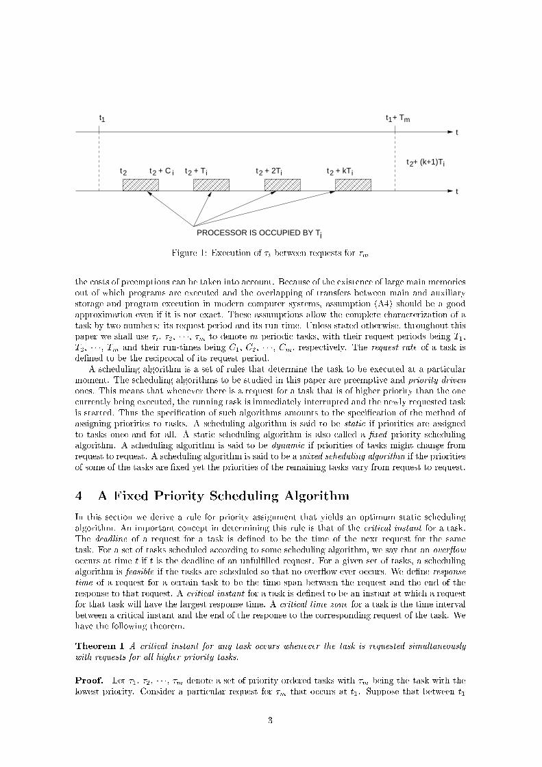
Figure 1: Execution of �i between requests for �m

the costs of preemptions can be taken into account. Because of the existence of large main memories

out of which programs are executed and the overlapping of transfers between main and auxiliary

storage and program execution in modern computer systems, assumption (A4) should be a good

approximation even if it is not exact. These assumptions allow the complete characterization of a

task by two numbers: its request period and its run-time. Unless stated otherwise, throughout this

paper we shall use �i, �2, � � �, �m to denote m periodic tasks, with their request periods being T1,

T2, � � �, Tm and their run-times being C1, C2, � � �, Cm, respectively. The request rate of a task is

de�ned to be the reciprocal of its request period.

A scheduling algorithm is a set of rules that determine the task to be executed at a particular

moment. The scheduling algorithms to be studied in this paper are preemptive and priority driven

ones. This means that whenever there is a request for a task that is of higher priority than the one

currently being executed, the running task is immediately interrupted and the newly requested task

is started. Thus the speci�cation of such algorithms amounts to the speci�cation of the method of

assigning priorities to tasks. A scheduling algorithm is said to be static if priorities are assigned

to tasks once and for all. A static scheduling algorithm is also called a �xed priority scheduling

algorithm. A scheduling algorithm is said to be dynamic if priorities of tasks might change from

request to request. A scheduling algorithm is said to be amixed scheduling algorithm if the priorities

of some of the tasks are �xed yet the priorities of the remaining tasks vary from request to request.

4 A Fixed Priority Scheduling Algorithm

In this section we derive a rule for priority assignment that yields an optimum static scheduling

algorithm. An important concept in determining this rule is that of the critical instant for a task.

The deadline of a request for a task is de�ned to be the time of the next request for the same

task. For a set of tasks scheduled according to some scheduling algorithm, we say that an over ow

occurs at time t if t is the deadline of an unful�lled request. For a given set of tasks, a scheduling

algorithm is feasible if the tasks are scheduled so that no over ow ever occurs. We de�ne response

time of a request for a certain task to be the time span between the request and the end of the

response to that request. A critical instant for a task is de�ned to be an instant at which a request

for that task will have the largest response time. A critical time zone for a task is the time interval

between a critical instant and the end of the response to the corresponding request of the task. We

have the following theorem.

Theorem 1 A critical instant for any task occurs whenever the task is requested simultaneously

with requests for all higher priority tasks.

Proof. Let �1, �2, � � �, �m denote a set of priority-ordered tasks with �m being the task with the

lowest priority. Consider a particular request for �m that occurs at t1. Suppose that between t1

3

��

��

��T1

1 2 3 4 5t

��

�� t51

T2

CRITICAL TIME ZONE

��

��

��

��

��

��T1

1 2 3 4 5t

��

��

t51

T2

CRITICAL TIME ZONE

��

��

��

T25

t

tT1

2

CRITICAL TIME ZONE

(c)

(a) (b)

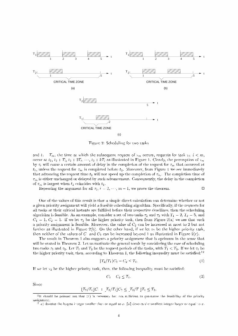
Figure 2: Scheduling for two tasks

and t1 + Tm, the time at which the subsequent request of �m occurs, requests for task �i, i < m,

occur at t2, t2 + Ti, t2 + 2Ti, � � �, t2 + kTi as illustrated in Figure 1. Clearly, the preemption of �mby �i will cause a certain amount of delay in the completion of the request for �m that occurred at

t1, unless the request for �m is completed before t2. Moreover, from Figure 1 we see immediately

that advancing the request time t2 will not speed up the completion of �m. The completion time of

�m is either unchanged or delayed by such advancement. Consequently, the delay in the completion

of �m is largest when t2 coincides with t1.

Repeating the argument for all �i, i = 2, � � �, m� 1, we prove the theorem. 2

One of the values of this result is that a simple direct calculation can determine whether or not

a given priority assignment will yield a feasible scheduling algorithm. Speci�cally, if the requests for

all tasks at their critical instants are ful�lled before their respective deadlines, then the scheduling

algorithm is feasible. As an example, consider a set of two tasks �1 and �2 with T1 = 2, T2 = 5, and

C1 = 1, C2 = 1. If we let �1 be the higher priority task, then from Figure 2(a) we see that such

a priority assignment is feasible. Moreover, the value of C2 can be increased at most to 2 but not

further as illustrated in Figure 2(b). On the other hand, if we let �2 be the higher priority task,

then neither of the values of C1 and C2 can be increased beyond 1 as illustrated in Figure 2(c).

The result in Theorem 1 also suggests a priority assignment that is optimum in the sense that

will be stated in Theorem 2. Let us motivate the general result by considering the case of scheduling

two tasks �1 and �2. Let T1 and T2 be the request periods of the tasks, with T1 < T2. If we let �1 be

the higher priority task, then, according to Theorem 1, the following inequality must be satis�ed:12

bT2=T1cC1 + C2 � T2: (1)

If we let �2 be the higher priority task, then, the following inequality must be satis�ed:

C1 + C2 � T1: (2)

Since

bT2=T1cC1 + bT2=T1cC2 � bT2=T1cT1 � T2;

1It should be pointed out that (1) is necessary but not suÆcient to guarantee the feasibility of the priority

assignment.2bxc denotes the largest integer smaller than or equal to x. dxe denotes the smallest integer larger or equal to x.

4

(2) implies (1). In other words, whenever the T1 < T2 and C1, C2 are such that the task scheduling

is feasible with �2 at higher priority than �1, it it also feasible with �1 at higher priority than �2.

Hence, more generally, it seems that a \reasonable" rule of priority assignment is to assign priorities

to tasks according to their request rates, independent of their run-times. Speci�cally, tasks with

higher request rates will have higher priorities. Such an assignment of priorities will be known as

the rate-monotonic priority assignment. As it turns out, such a priority assignment is optimum

in the sense that no other �xed priority assignment rule can schedule a task set which cannot be

scheduled by the rate-monotonic priority assignment.

Theorem 2 If a feasible priority assignment exists for some task set, the rate-monotonic priority

is feasible for that task set.

Proof. Let �1, �2, � � �, �m be a set of m tasks with a certain feasible priority assignment. Let �iand �j be two tasks of adjacent priorities in such an assignment with �i being the higher priority

one. Suppose that Ti > Tj . Let us interchange the priorities of �i and �j . It is not diÆcult to see

that the resultant priority assignment is still feasible. Since the rate-monotonic priority assignment

can be obtained from any priority ordering by a sequence of pairwise priority reorderings as above,

we prove the theorem. 2

5 Achievable Processor Utilization

At this point, the tools are available to determine a least upper bound to processor utilization in

�xed priority systems. We de�ne the (processor) utilization factor to be the fraction of processor

time spent in the execution of the task set. In other words, the utilization factor is equal to one

minus the fraction of idle processor time. Since Ci=Ti is the fraction of processor time spent in

executing task �i, for m tasks, the utilization factor is:

U =

mX

i=1

(Ci=Ti)

Although the processor utilization factor can be improved by increasing the values of the Ci's or

by decreasing the values of the Ti's, it is upper bounded by the requirement that all tasks satisfy

their deadlines at their critical instants. It is clearly uninteresting to ask how small the processor

utilization factor can be. Let us be precise about what we mean. Corresponding to a priority

assignment, a set of tasks is said to fully utilize the processor if the priority assignment is feasible

for the set and if an increase in the run-time of any of the tasks in the set will make the priority

assignment infeasible. For a given �xed priority scheduling algorithm, the least upper bound of the

utilization factor is the minimum of the utilization factors over all sets of tasks that fully utilize

the processor. For all task sets whose processor utilization factor is below this bound, there exists

a �xed priority assignment which is feasible. On the other hand, utilization above this bound can

only be achieved if the Ti of the tasks are suitably related.

Since the rate-monotonic priority assignment is optimum, the utilization factor achieved by the

rate-monotonic priority assignment for a given task set is greater than or equal to the utilization fac-

tor for any other priority assignment for that task set. Thus, the least upper bound to be determined

is the in�mum of the utilization factors corresponding to the rate-monotonic priority assignment

over all possible request periods and run-times for the tasks. The bound is �rst determined for two

tasks, then extended for an arbitrary number of tasks.

Theorem 3 For a set of two tasks with �xed priority assignment, the least upper bound to the

processor utilization factor is U = 2(212 � 1).

5

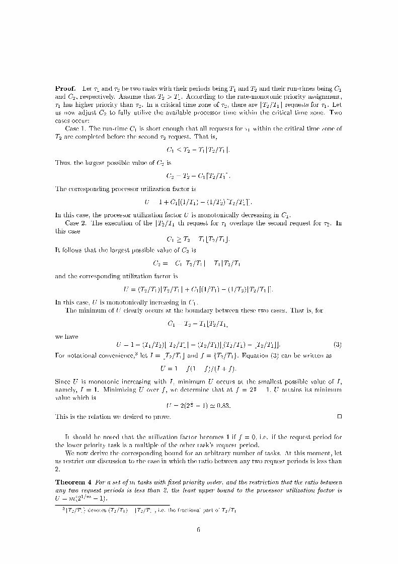
Proof. Let �1 and �2 be two tasks with their periods being T1 and T2 and their run-times being C1

and C2, respectively. Assume that T2 > T1. According to the rate-monotonic priority assignment,

�1 has higher priority than �2. In a critical time zone of �2, there are dT2=T1e requests for �1. Let

us now adjust C2 to fully utilize the available processor time within the critical time zone. Two

cases occur:

Case 1. The run-time C1 is short enough that all requests for �1 within the critical time zone of

T2 are completed before the second �2 request. That is,

C1 � T2 � T1bT2=T1c:

Thus, the largest possible value of C2 is

C2 = T2 � C1dT2=T1e:

The corresponding processor utilization factor is

U = 1 + C1[(1=T1)� (1=T2)dT2=T1e]:

In this case, the processor utilization factor U is monotonically decreasing in C1.

Case 2. The execution of the dT2=T1eth request for �1 overlaps the second request for �2. In

this case

C1 � T2 � T1bT2=T1c:

It follows that the largest possible value of C2 is

C2 = �C1bT2=T1c+ T1bT2=T1c

and the corresponding utilization factor is

U = (T2=T1)bT2=T1c+ C1[(1=T1)� (1=T2)bT2=T1c]:

In this case, U is monotonically increasing in C1.

The minimum of U clearly occurs at the boundary between these two cases. That is, for

C1 = T2 � T1bT2=T1c

we have

U = 1� (T1=T2)[dT2=T1e � (T2=T1)][(T2=T1)� bT2=T1c]: (3)

For notational convenience,3 let I = bT2=T1c and f = fT2=T1g. Equation (3) can be written as

U = 1� f(1� f)=(I + f):

Since U is monotonic increasing with I , minimum U occurs at the smallest possible value of I ,

namely, I = 1. Minimizing U over f , we determine that at f = 212 � 1, U attains its minimum

value which is

U = 2(212 � 1) ' 0:83:

This is the relation we desired to prove. 2

It should be noted that the utilization factor becomes 1 if f = 0, i.e. if the request period for

the lower priority task is a multiple of the other task's request period.

We now derive the corresponding bound for an arbitrary number of tasks. At this moment, let

us restrict our discussion to the case in which the ratio between any two request periods is less than

2.

Theorem 4 For a set of m tasks with �xed priority order, and the restriction that the ratio between

any two request periods is less than 2, the least upper bound to the processor utilization factor is

U = m(21=m � 1).

3fT2=T1g denotes (T2=T1)� bT2=T1c, i.e. the fractional part of T2=T1

6

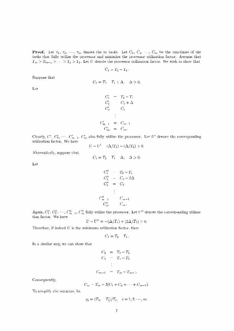
Proof, Let �1, �2, � � �, �m denote the m tasks. Let C1, C2, � � �, Cm be the run-times of the

tasks that fully utilize the processor and minimize the processor utilization factor. Assume that

Tm > Tm�1 > � � � > T2 > T1. Let U denote the processor utilization factor. We wish to show that

C1 = T2 � T1:

Suppose that

C1 = T2 � T1 +�; � > 0:

Let

C0

1 = T2 � T1

C0

2 = C2 +�

C0

3 = C3

...

C0

m�1 = Cm�1

C0

m = Cm:

Clearly, C 0

1, C0

2, � � �, C0

m�1, C0

m also fully utilize the processor. Let U 0 denote the corresponding

utilization factor. We have

U � U0 = (�=T1)� (�=T2) > 0:

Alternatively, suppose that

C1 = T2 � T1 ��; � > 0:

Let

C00

1 = T2 � T1

C00

2 = C2 � 2�

C00

3 = C3

...

C00

m�1 = Cm�1

C00

m = Cm:

Again, C 00

1 , C00

2 , � � �, C00

m�1, C00

m fully utilize the processor. Let U 00 denote the corresponding utiliza-

tion factor. We have

U � U00 = �(�=T1) + (2�=T1) > 0:

Therefore, if indeed U is the minimum utilization factor, then

C1 = T2 � T1:

In a similar way, we can show that

C2 = T3 � T2

C4 = T4 � T3

...

Cm�1 = Tm � Tm�1:

Consequently,

Cm = Tm � 2(C1 + C2 + � � �+ Cm�1):

To simplify the notation, let

gi = (Tm � Ti)=Ti; i = 1; 2; � � � ;m:

7

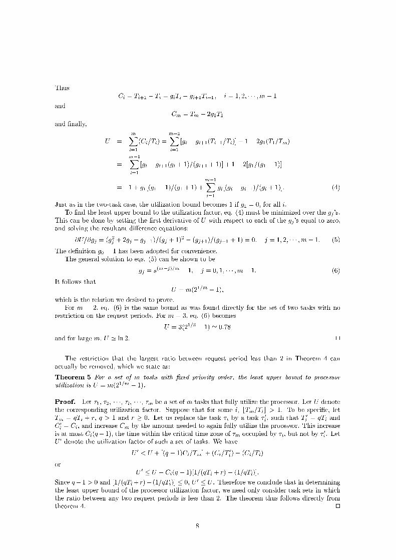
Thus

Ci = Ti+1 � Ti = giTi � gi+1Ti+1; i = 1; 2; � � � ;m� 1

and

Cm = Tm � 2g1T1

and �nally,

U =

mX

i=1

(Ci=Ti) =

m�1X

i=1

[gi � gi+1(Ti+1=Ti)] + 1� 2g1(T1=Tm)

=

m�1X

i=1

[gi � gi+1(gi + 1)=(gi+1 + 1)] + 1� 2[g1=(g1 + 1)]

= 1 + g1[(g1 � 1)=(g1 + 1) +

m�1X

i=1

gi[(gi � gi�1)=(gi + 1)]: (4)

Just as in the two-task case, the utilization bound becomes 1 if g1 = 0, for all i.

To �nd the least upper bound to the utilization factor, eq. (4) must be minimized over the gj 's.

This can be done by setting the �rst derivative of U with respect to each of the gj 's equal to zero,

and solving the resultant di�erence equations:

@U=@gj = (g2j + 2gj � gj�1)=(gj + 1)2 � (gj+1)=(gj+1 + 1) = 0; j = 1; 2; � � � ;m� 1: (5)

The de�nition g0 = 1 has been adopted for convenience.

The general solution to eqs. (5) can be shown to be

gj = s(m�j)=m

� 1; j = 0; 1; � � � ;m� 1: (6)

It follows that

U = m(21=m � 1);

which is the relation we desired to prove.

For m = 2, eq. (6) is the same bound as was found directly for the set of two tasks with no

restriction on the request periods. For m = 3, eq. (6) becomes

U = 3(21=3 � 1) ' 0:78

and for large m, U ' ln 2. 2

The restriction that the largest ratio between request period less than 2 in Theorem 4 can

actually be removed, which we state as:

Theorem 5 For a set of m tasks with �xed priority order, the least upper bound to processor

utilization is U = m(21=m � 1).

Proof. Let �1, �2, � � �, �i, � � �, �m be a set of m tasks that fully utilize the processor. Let U denote

the corresponding utilization factor. Suppose that for some i, bTm=Tic > 1. To be speci�c, let

Tm = qTi + r, q > 1 and r � 0. Let us replace the task �i by a task �0

i , such that T 0

i = qTi and

C0

i = Ci, and increase Cm by the amount needed to again fully utilize the processor. This increase

is at most Ci(q� 1), the time within the critical time zone of �m occupied by �i, but not by �0

i . Let

U0 denote the utilization factor of such a set of tasks. We have

U0

< U + [(q � 1)Ci=Tm] + (Ci=T0

i )� (Ci=Ti)

or

U0

� U + Ci(q � 1)[1=(qTi + r) � (1=qTi)]:

Since q�1 > 0 and [1=(qTi+ r)� (1=qTi)] � 0, U 0

� U . Therefore we conclude that in determining

the least upper bound of the processor utilization factor, we need only consider task sets in which

the ratio between any two request periods is less than 2. The theorem thus follows directly from

theorem 4. 2

8

��

��

PROCESSORIDLE-PERIOD

REQUESTS FORTASK 2

REQUESTS FORTASK 3

REQUESTS FORTASK m

REQUESTS FORTASK 1

��

��

��

��

��

��

��

��

��

��

��

��

��

��

��

��

��

t3t2t1

....

a

b

c

m

0

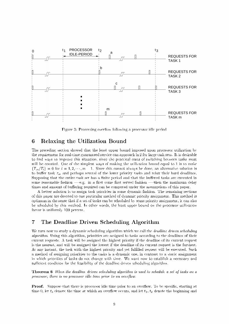
Figure 3: Processing over ow following a processor idle period

6 Relaxing the Utilization Bound

The preceding section showed that the least upper bound imposed upon processor utilization by

the requirement for real-time guaranteed service can approach ln 2 for large task sets. It is desirable

to �nd ways to improve this situation, since the practical costs of switching between tasks must

still be counted. One of the simplest ways of making the utilization bound equal to 1 is to make

fTm=Tig = 0 for i = 1; 2; � � � ;m � 1. Since this cannot always be done, an alternative solution is

to bu�er task �m and perhaps several of the lower priority tasks and relax their hard deadlines.

Supposing that the entire task set has a �nite period and that the bu�ered tasks are executed in

some reasonable fashion | e.g. in a �rst come �rst served fashion | then the maximum delay

times and amount of bu�ering required can be computed under the assumptions of this paper.

A better solution is to assign task priorities in some dynamic fashion. The remaining sections

of this paper are devoted to one particular method of dynamic priority assignment. This method is

optimum in the sense that if a set of tasks can be scheduled by some priority assignment, it can also

be scheduled by this method. In other words, the least upper bound on the processor utilization

factor is uniformly 100 percent.

7 The Deadline Driven Scheduling Algorithm

We turn now to study a dynamic scheduling algorithm which we call the deadline driven scheduling

algorithm. Using this algorithm, priorities are assigned to tasks according to the deadlines of their

current requests. A task will be assigned the highest priority if the deadline of its current request

is the nearest, and will be assigned the lowest if the deadline of its current request is the furthest.

At any instant, the task with the highest priority and yet ful�lled request will be executed. Such

a method of assigning priorities to the tasks is a dynamic one, in contrast to a static assignment

in which priorities of tasks do not change with time. We want now to establish a necessary and

suÆcient condition for the feasibility of the deadline driven scheduling algorithm.

Theorem 6 When the deadline driven scheduling algorithm is used to schedule a set of tasks on a

processor, there is no processor idle time prior to an over ow.

Proof. Suppose that there is processor idle time prior to an over ow. To be speci�c, starting at

time 0, let t3 denote the time at which an over ow occurs, and let t1, t2 denote the beginning and

9

��

a2

��

a3

��

b1

��

b2

��

b3

...

��

��

��a1

0 T

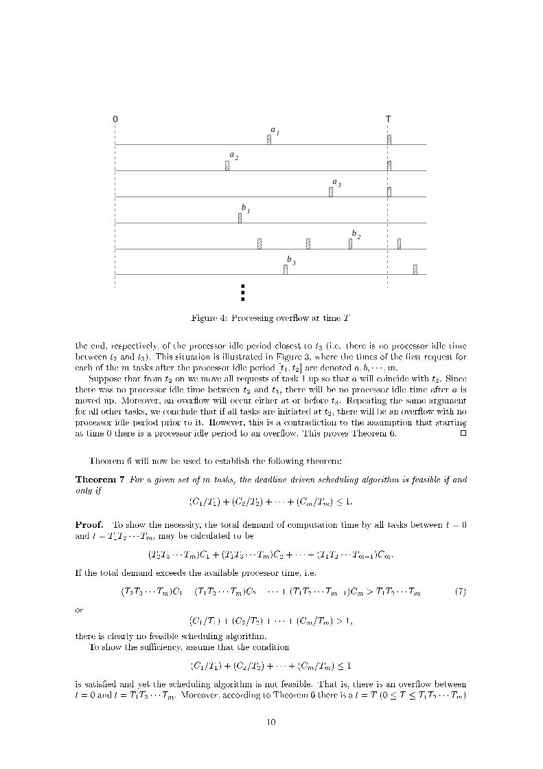
Figure 4: Processing over ow at time T

the end, respectively, of the processor idle period closest to t3 (i.e. there is no processor idle time

between t2 and t3). This situation is illustrated in Figure 3, where the times of the �rst request for

each of the m tasks after the processor idle period [t1; t2] are denoted a; b; � � � ;m.

Suppose that from t2 on we move all requests of task 1 up so that a will coincide with t2. Since

there was no processor idle time between t2 and t3, there will be no processor idle time after a is

moved up. Moreover, an over ow will occur either at or before t3. Repeating the same argument

for all other tasks, we conclude that if all tasks are initiated at t2, there will be an over ow with no

processor idle period prior to it. However, this is a contradiction to the assumption that starting

at time 0 there is a processor idle period to an over ow. This proves Theorem 6. 2

Theorem 6 will now be used to establish the following theorem:

Theorem 7 For a given set of m tasks, the deadline driven scheduling algorithm is feasible if and

only if

(C1=T1) + (C2=T2) + � � �+ (Cm=Tm) � 1:

Proof. To show the necessity, the total demand of computation time by all tasks between t = 0

and t = T1T2 � � �Tm, may be calculated to be

(T2T3 � � �Tm)C1 + (T1T3 � � �Tm)C2 + � � �+ (T1T2 � � �Tm�1)Cm:

If the total demand exceeds the available processor time, i.e.

(T2T3 � � �Tm)C1 + (T1T3 � � �Tm)C2 + � � �+ (T1T2 � � �Tm�1)Cm > T1T2 � � �Tm (7)

or

(C1=T1) + (C2=T2) + � � �+ (Cm=Tm) > 1;

there is clearly no feasible scheduling algorithm.

To show the suÆciency, assume that the condition

(C1=T1) + (C2=T2) + � � �+ (Cm=Tm) � 1

is satis�ed and yet the scheduling algorithm is not feasible. That is, there is an over ow between

t = 0 and t = T1T2 � � �Tm. Moreover, according to Theorem 6 there is a t = T (0 � T � T1T2 � � �Tm)

10

�� a2

��

a3

��

b1

��

b2

��

b3

REQUESTS WITH DEALINES AT ANDWERE FULFILLED BEFORE

a aT ’

1 3

��

��

��

��

�� a1

T ’ T0

Figure 5: Processing over ow at time T without execution of fbig following T0

at which there is an over ow with no processor idle time between t = 0 and t = T . To be speci�c,

let a1, a2, � � �, b1, b2, � � �, denote the request times of the m tasks immediately prior to T , where

a1, a2, � � � are the request times of tasks with deadlines at T , and b1, b2, � � � are the request times

of tasks with deadlines beyond T . This is illustrated in Figure 4.

Two cases must be examined.

Case 1. None of the computations requested at b1, b2, � � � was carried out before T . In this case,

the total demand of computation time between 0 and T is

bT=T1cC1 + bT=T2cC2 + � � �+ bT=TmcCm:

Since there is no processor idle period,

bT=T1cC1 + bT=T2cC2 + � � �+ bT=TmcCm > T:

Also, since x � bxc for all x,

(T=T1)C1 + (T=T2)C2 + � � �+ (T=Tm)Cm > T

and

(C1=T1) + (C2=T2) + � � �+ (Cm=Tm) > 1;

which is a contradiction to (7).

Case 2. Some of the computations requested at b1, b2, � � � were carried out before T . Since an

over ow occurs at T , there must exist a point T 0 such that none of the requests at b1, b2, � � � was

carried out within the interval T 0

� t � T . In other words, within T0

� t � T , only those requests

with deadlines at or before T will be executed, as illustrated in Figure 5. Moreover, the fact that

one or more of the tasks having requests at the bi's is executed until t = T0 means that all those

requests initiated before T 0 with deadlines at or before T have been ful�lled before T 0. Therefore,

the total demand of processor time within T0

� t � T is less than or equal to

b(T � T0)=T1cC1 + b(T � T

0)=T2cC2 + � � �+ b(T � T0)=TmcCm:

That an over ow occurs at T means that

b(T � T0)=T1cC1 + b(T � T

0)=T2cC2 + � � �+ b(T � T0)=TmcCm > T � T

0

;

11

which implies again

(C1=T1) + (C2=C2) + � � �+ (Cm=Tm) > 1;

and which is a contradiction to (7). This proves the theorem. 2

As was pointed out above, the deadline driven scheduling algorithm is optimum in the sense

that if a set of tasks can be scheduled by any algorithm, it can be scheduled by the deadline driven

scheduling algorithm.

8 A Mixed Scheduling Algorithm

In this section we investigate a class of scheduling algorithms which are combinations of the rate-

monotonic scheduling algorithm and the deadline driven scheduling algorithm. We call an algorithm

in this class a mixed scheduling algorithm. The study of the mixed scheduling algorithm is motivated

by the observation that the interrupt hardware of present day computers acts as a �xed priority

scheduler and does not appear to be compatible with a hardware dynamic scheduler. On the other

hand, the cost of implementing a software scheduler for the slower paced tasks is not signi�cantly

increased if these tasks are deadline driven instead of having a �xed priority assignment. To be

speci�c, let tasks 1, 2, � � �, k, the k tasks of shortest periods, be scheduled according to the �xed

priority rate-monotonic scheduling algorithm, and let the remaining tasks, tasks k + 1, k + 2, � � �,

m, be scheduled according to the deadline driven scheduling algorithm when the processor is not

occupied by tasks 1, 2, � � �, k.

Let a(t) be a nondecreasing function of t. We say that a(t) is sublinear if for all t and all T

a(T ) � a(t+ T )� a(t)

The availability function of a processor for a set of tasks is de�ned as the accumulated processor

time from 0 to t available to this set of tasks. Suppose that k tasks have been scheduled on a

processor by a �xed priority scheduling algorithm. Let ak(t) denote the availability function of the

processor for tasks k + 1, k + 2, � � �, m. Clearly, ak(t) is a nondecreasing function of t. Moreover,

ak(t) can be shown to be sublinear by means of the critical time zone argument. We have:

Theorem 8 If a set of tasks are scheduled by the deadline driven scheduling algorithm on a pro-

cessor whose availability function is sublinear, then there is no processor idle period to an over ow.

Proof. Similar to that of Theorem 6. 2

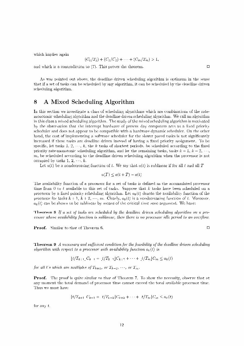
Theorem 9 A necessary and suÆcient condition for the feasibility of the deadline driven scheduling

algorithm with respect to a processor with availability function ak(t) is

bt=Tk+1cCk+1 + bt=Tk+2cCk+2 + � � �+ bt=TmcCm � ak(t)

for all t's which are multiples of Tk+1, or Tk+2, � � �, or Tm.

Proof. The proof is quite similar to that of Theorem 7. To show the necessity, observe that at

any moment the total demand of processor time cannot exceed the total available processor time.

Thus we must have

bt=Tk+1cCk+1 + bt=Tk+2cCk+2 + � � �+ bt=TmcCm � ak(t)

for any t.

12

To show the suÆciency, assume that the condition stated in the theorem is satis�ed and yet

there is an over ow at T . Examine the two cases considered in the proof of Theorem 7. For case 1,

bT=Tk+1cCk+1 + bT=Tk+2cCk+2 + � � �+ bT=TmcCm > ak(T );

which is a contradiction to the assumption. Note that T is multiple of Tk+1, or Tk+2, � � �, or Tm.

For case 2,

b(T � T0)=Tk+1cCk+1 + b(T � T

0)=Tk+2cCk+2 + � � �+

b(T � T0)=TmcCm > ak(T � T

0)

Let � be the smallest nonnegative number such that T � T0

� � is a multiple of Tk+1, or Tk+2, � � �,

or Tm. Clearly,

b(T � T0

� �)=Tk+jc = b(T � T0)=Tk+jc for each j = 1; 2; � � � ;m� k

and thus

b(T � T0

� �)=Tk+1cCk+1 + b(T � T0

� �)=Tk+2cCk+2 + � � �+

b(T � T0

� �)=TmcCm > ak(T � T0) � ak(T � T

0

� �);

which is a contradiction to the assumption. This proves the theorem. 2

Although the result in Theorem 9 is a useful general result, its application involves the solution

of a large set of inequalities. In any speci�c case, it may be advantageous to derive suÆcient

conditions on schedule feasibility rather than work directly from Theorem 9. As an example,

consider the special case in which three tasks are scheduled by the mixed scheduling algorithm such

that the task with the shortest period is assigned a �xed and highest priority, and the other two

tasks are scheduled by the deadline driven scheduling algorithm. It may be readily veri�ed that if

1� (C1=T1)�min[(T1 � C1)=T2; (C1=T1)] � (C2=T2) + (C3=T3);

then the mixed scheduling algorithm is feasible. It may be also veri�ed that if

C2 � a1(T2); bT3=T2cC2 + C3 � a1(bT3=T2cT2); and

(bT3=T2c+ 1)C2 + C3 � a1(T3);

then the mixed scheduling algorithm is feasible.

The proof of these statements consists of some relatively straightforward but extensive inequality

manipulation, and may be found in Liu [13]. Unfortunately, both of these suÆcient conditions cor-

respond to considerably lower processor utilization than does the necessary and suÆcient condition

of Theorem 9.

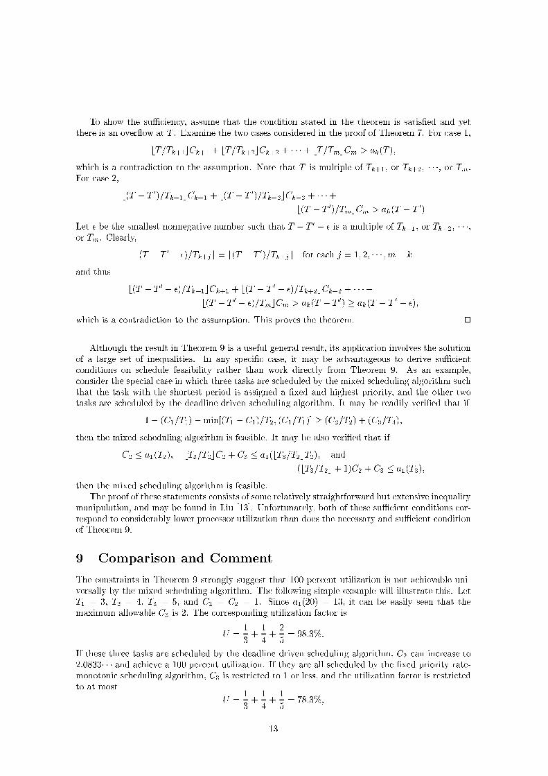
9 Comparison and Comment

The constraints in Theorem 9 strongly suggest that 100 percent utilization is not achievable uni-

versally by the mixed scheduling algorithm. The following simple example will illustrate this. Let

T1 = 3, T2 = 4, T3 = 5, and C1 = C2 = 1. Since a1(20) = 13, it can be easily seen that the

maximum allowable C3 is 2. The corresponding utilization factor is

U =1

3+

1

4+

2

5= 98:3%:

If these three tasks are scheduled by the deadline driven scheduling algorithm, C2 can increase to

2.0833� � � and achieve a 100 percent utilization. If they are all scheduled by the �xed priority rate-

monotonic scheduling algorithm, C3 is restricted to 1 or less, and the utilization factor is restricted

to at most

U =1

3+

1

4+

1

5= 78:3%;

13

which is only slightly greater than the worst case three task utilization bound.

Although a closed form expression for the least upper bound to processor utilization has not

been found for the mixed scheduling algorithm, this example strongly suggests that the bound is

considerably less restrictive for the mixed scheduling algorithm than for the �xed priority rate-

monotonic scheduling algorithm. The mixed scheduling algorithm may thus be appropriate for

many applications.

10 Conclusion

In the initial parts of this paper, �ve assumptions were made to de�ne the environment which

supported the remaining analytical work. Perhaps the most important and least defensible of these

are (A1), that all tasks have periodic requests, and (A4), that run-times are constant. If these do

not hold, the critical time zone for each task should be de�ned as the time zone between its request

and deadline during which the maximum possible amount of computation is performed by the tasks

having higher priority. Unless detailed knowledge of the run-time and request are available, run-

ability constraints on task run-times would have to be computed on the basis of assumed periodicity

and constant run-time, using a period equal to the shortest request interval and a run-time equal to

the longest run-time. None of our analytic work would remain valid under this circumstance, and

a severe bound on processor utilization could well be imposed by the task aperiodicity. The �xed

priority ordering now is monotonic with the shortest span between request and deadline for each

task instead of with the unde�ned request period. The same will be true if some of the deadlines are

tighter than assumed in (A2), although the impact on utilization will be slight if only the highest

priority tasks are involved. It would appear that the value of the implications of (A1) and (A4) are

great enough to make them a design goal for any real-time tasks which must receive guaranteed

service.

In conclusion, this paper has discussed some of the problems associated with multiprogramming

in a hard-real-time environment typi�ed by process control and monitoring, using some assumptions

which seem to characterize that application. A scheduling algorithm which assigns priorities to

tasks in a monotonic relation to their request rates was shown to be optimum among the class

of all �xed priority scheduling algorithms. The least upper bound to processor utilization factor

for this algorithm is on the order of 70 percent for large task sets. The dynamic deadline driven

scheduling algorithm was then shown to be globally optimum and capable of achieving full processor

utilization. A combination of the two scheduling algorithms was then discussed; this appears to

provide most of the bene�ts of the deadline driven scheduling algorithm, and yet may be readily

implemented in existing computers.

References

[1] Manacher, G. K. Production and stabilization of real{time task schedules. J. ACM 14, 3

(July 1967), 439{465.

[2] McKinney, J. M. A survey of analytical time-sharing models. Computing Surveys 1, 2 (June

1969), 105{116.

[3] Codd, E. F. Multiprogramming scheduling. Comm. ACM 3, 6, 7 (June, July 1960), 347{350;

413{418.

[4] Heller, J. Sequencing aspects of multiprogramming. J. ACM 8, 3 (July 1961), 426{439.

[5] Graham, R. L. Bounds for certain multiprocessing anomalies. Bell System Tech. J. 45, 9

(Nov. 1966), 1563{1581.

[6] Oschner, B. P., and Coffman, E. G., Jr. Controlling a multiprocessor system. Bell Labs

Record 44, 2 (Feb. 1966).

14

[7] Muntz, R. R., and Coffman, E.G., Jr. Preemptive scheduling of real{time tasks on

multiprocessor systems. J. ACM 17, 2 (Apr. 1970), 324{338.

[8] Bernstein, A. J.., and Sharp, J. C. A policy{driven scheduler for a time{sharing system.

Comm. ACM 14, 2 (Feb. 1971), 74{78.

[9] Lampson, B. W. A scheduling philosophy for multiprocessing systems. Comm. ACM 11, 5

(May, 1968), 347{360.

[10] Martin, J. Programming Real-Time Computer Systems. Prentice{Hall, Englewood Cli�s, N.

J., 1965.

[11] Jirauch, D. H. Software design techniques for automatic checkout. IEEE Trans. AES 3, 6

(Nov. 1967), 934{940.

[12] Martin, J. Op. cit., p.35 �.

[13] Liu, C. L. Scheduling algorithms for hard-real-time multiprogramming of a single proces-

sor. JPL Space Programs Summary 37{60, Vol. II, Jet Propulsion Lab., Calif. Inst. of Tech.,

Pasadena, Calif., Nov. 1969.

15

Scheduling Algorithms for Multiprogramming in a Hard-Real ...

Documents

Transcript of Scheduling Algorithms for Multiprogramming in a Hard-Real ...