Locally Optimized Scheduling and Power ControlAlgorithms for Multi-hop Wireless Networks under

SINR Interference ModelsJoohwan Kim, Xiaojun Lin, and Ness B. Shroff

Center for Wireless Systems and Applications (CWSA)School of Electrical and Computer Engineering, Purdue University

West Lafayette, IN 47907, U.S.AEmail:{jhkim, linx, shroff}@purdue.edu

Abstract— In this paper, we develop locally optimized schedul-ing and power control algorithms for multi-hop wireless networksunder SINR interference models. Our scheme can be implementedin a fully distributed manner and requires only that eachnode solve a simple local optimization problem. Since, in ouralgorithms, each node operates independently of other nodes, itneeds to predict the behavior of neighboring nodes when carryingout its local optimization. For such prediction, our proposed algo-rithms exploit the past records of neighboring nodes’ schedulingand power control decisions. Through simulations, we show thatour algorithms significantly outperform the state-of-the-art.

I. INTRODUCTION

In this paper, we develop efficient scheduling and powercontrol algorithms that support high data rates in multi-hop wireless networks. In recent years, throughput-optimalscheduling and power control algorithms that maximize theachievable throughput of multi-hop wireless networks havebeen extensively studied in the literature [1], [2], [3]. How-ever, these throughput-optimal algorithms are often difficult toimplement mainly because of the following reasons: first, theoptimal algorithm operates in a fully centralized manner. Thus,a centralized scheduler needs to collect global information ofthe queue lengths from the entire network and to distributeits scheduling and power control decision back to the entirenetwork. Both information collection and decision distributioncould result in significant communication overhead. Second,these throughput-optimal algorithms require the centralizedscheduler to solve a complex global optimization problem,whose complexity could exponentially increase in the networksize.

There have been recent efforts to develop efficient schedul-ing algorithms that alleviate the communication and compu-tation overheads. Progress has been made under restrictiveclasses of interference models. A commonly used model is theK-hop interference model, in which two links that are withinK-hops of each other cannot simultaneously communicate,and the capacity of a link is a constant value if there is nointerference [4], [5], [6], [7], [8], [9], [10]. In [4], the MaximalMatching (MM) scheduling algorithm is used under the node-exclusive interference model (the special case of the K-hop

interference model with K = 1.) This algorithm can operatein a distributed fashion and is proven to have at least onehalf of the achievable throughput under the node-exclusiveinterference model. These features have motivated subsequentresearch on the distributed algorithms with provable perfor-mance [5], [6], [7], [8], [9], [10].

However, the K-hop interference models do not adequatelycapture the more realistic Signal-to-Interference-and-Noise-Ratio (SINR) interference models, where link capacities couldvary according to the signal and the interference levels. Inthis paper, we consider the following two SINR interferencemodels that are commonly used: the linear SINR interferencemodel and the logarithmic SINR interference model. Under thelinear SINR interference model, the capacity of each link islinearly proportional to the SINR value. In contrast, under thelogarithmic SINR interference model, the capacity of a link isrepresented as a logarithmic function of the SINR value.

Scheduling algorithms under the different types of SINRinterference models have been studied in the literature [3],[11], [12], [13]. In [3], the authors have proposed a simpleand distributed scheduling algorithm that is an approximationto the optimal “Dynamic Routing and Power Control” (DRPC)algorithm (which is centralized and requires high computa-tional complexity) and could run under both the linear andthe logarithmic SINR interference models. In [11], for thelogarithmic SINR interference model the author has proposedthe “Jointly Optimal Congestion-control and Power-control”(JOCP) algorithm that is distributed and optimal under theassumption that SINR values are high. The authors in [12] and[13] have also proposed heuristic algorithms under the targetSINR interference model where the capacity of a link is aconstant value when the received SINR exceeds a threshold,or zero otherwise.

In this paper, we propose new distributed scheduling andpower control algorithms under SINR interference models andcompare their performance to the state-of-the-art in [3] and[11]. We show that our algorithms have constant complexity,consume a constant amount of computation time at each timeslot, and operate in a fully distributed manner. In fact, the

complexity of our algorithms is independent of the size of thenetwork.

The rest of this paper is organized as follows. Section IIillustrates the system model, including our SINR interferencemodels, and reviews the fundamentals. Section III develops alocally-optimized scheduling algorithm under the linear SINRinterference model. Section IV extends our result in SectionIII to the logarithmic SINR interference model. Here, thescheduling algorithm developed in Section III is generalized tohave power control capability. Section V provides simulationresults that compare the performance of our algorithms withthe optimal performance. We also provide extensive compar-ison to other algorithms under different SINR interferencemodels. We conclude in Section VI.

II. SYSTEM MODEL

In this paper, we consider a multi-hop wireless networkwith N nodes and L links. All nodes and links are assumedto be static. Each link l corresponds to a transmitting node,denoted by b(l), and a receiving node, denoted by e(l). LetN and L denote the set of all nodes and the set of all links,respectively. An outgoing link of node i is defined as a linkwhose transmitter is node i. We define the outgoing link setof node i as Li,out = {l ∈ L| b(l) = i} and the number ofoutgoing links of node i as Li,out. Similarly, an incoming linkof node i is a link whose receiver is node i. We define theincoming link set of node i as Li,in = {l ∈ L| e(l) = i}, andthe number of the incoming links of node i as Li,in.

We consider a time-slotted network. Let Pl(t) denote thetransmission power at the transmitter of link l at time slot t,and ~P (t) = [Pl(t), l ∈ L] be the power assignment vector attime slot t. Let Pi,max be the maximum power limit of eachtransmitting node i, such that 0 ≤

∑l∈Li,out

Pl(t) ≤ Pi,max.We assume that the link capacity is a function of its SINR

value. Let rl(t) be the capacity of link l at time slot t, andξl(t) be the measured SINR value at the receiver of link lat time slot t. Specifically, ξl(t) is the ratio of the receivedsignal power to the received interference and noise power, andis given by

ξl(t) =GllPl(t)∑

h∈L\{l} GhlPh(t) + ηl, (1)

where ηl denotes the time-invariant background noise at thereceiver of link l, and Ghl denotes the wireless channel gainfrom the transmitter of link h to the receiver of link l. Sincethe nodes are static, the channel gains are assumed to be fixedand known. (We do not consider fading effects here.) We thenconsider two types of functional relationships between rl(t)and ξl(t):

• The logarithmic SINR interference model: the capacityof link l is determined by rl(t) = B log(1+ξl(t)), whereB denotes the fixed channel bandwidth.

• The linear SINR interference model: the capacity oflink l is determined by rl(t) = Bξl(t). This model canbe viewed as an approximation of the logarithmic SINRinterference model, when the SINR level ξl(t) is low.

In this paper, we will first study the linear SINR interferencemodel due to its analytical simplicity, and then the logarithmicSINR interference model.

Remarks: In practical systems, there are often additionalconstraints on the feasible transmission patterns. For example,a node may not be able to receive when it is also transmitting.Also, a node may not be able to receive from multipletransmitters at the same time. Note that our model can beeasily adapted to these settings. For example, if a node cannotreceive when it is transmitting, we can simply set Ghl = ∞when the transmitter of link h is the same as the receiver oflink l, i.e., b(h) = e(l). Similarly, if a node cannot receive frommultiple transmitters simultaneously, we can set Ghl = ∞when the receiver nodes of link l and link h are the same, i.e,e(h) = e(l).

We assume that there are U users in the network whose datacould travel multiple links from their source nodes to theircorresponding destination nodes. Let λu be the data arrivalrate of user u at the source node. Let ~λ = [λ1, λ2, · · · , λU ].The capacity region under a scheduling and power controlalgorithm is defined as the set of vectors ~λ under which thenetwork remains stable. Here, stability means that all queuesremain finite. The algorithm that achieves the largest capacityregion is referred to as the throughput-optimal scheduling andpower control algorithm (or simply the optimal algorithm inthe rest of the paper). It has been proven in [1] that one suchoptimal algorithm computes the power-assignment vector attime slot t as the solution to the following global optimizationproblem;

~P ∗(t) = arg max~P∈Π

∑l∈L

rl(~P ) ql(t), (2)

where Π = {~P ; 0 ≤∑

l∈Li,outPl(t) ≤ Pi,max ∀i ∈ N}, and

ql(t) denotes the queue length of link l at time slot t.As mentioned in the Introduction, this optimal algorithm

is extremely difficult to implement due to the communicationoverhead (of collecting ql(t)’s and distributing ~P ∗(t)) and thecomputational overhead (of solving (2)).

III. A LOCALLY OPTIMIZED SCHEDULING ALGORITHMFOR THE LINEAR SINR INTERFERENCE MODEL

In this section, we propose a new distributed algorithm,the locally optimized scheduling algorithm, under the linearSINR interference model. Our algorithm may be viewed asa suboptimal approximation of the optimal algorithm (2).It significantly lowers the computation and communicationoverhead of the optimal algorithm.

A. Distributed Scheduler

Our goal is to develop a distributed scheduling and powercontrol algorithm under which each node schedules its ownresources in a distributed fashion. In other words, each nodeshould decide by itself whether it should transmit or not, and,if it transmits, to which adjacent nodes and at what power levelit should transmit. Note that under the linear SINR interferencemodel, it has been proven in [2] that the optimal schedulingdecision and power assignment are of the form that each node

should either transmit on only one of its outgoing links withthe node’s maximum power, or not transmit at all. Hence,for this interference model, we need to focus only on thescheduling decision. Let Si(t) denote the scheduling decisionof node i at time slot t, given by

Si(t) =

0, if node i does not schedule its outgoing

links,s, if node i schedules the s-th outgoing link

with power Pi,max (s = 1, · · · , Li,out).

Since each node i has Li,out outgoing links to schedule, it hasa total of Li,out + 1 choices of scheduling decisions.

B. Local Optimization

We propose to develop a distributed scheduler as an approx-imate solution to (2) as follows. We define the neighboringlinks of node i as the links that are close enough to node iso that node i can communicate basic information, such asthe queue lengths and SINR values, with these links directly.Let Li be the set of all neighboring links of node i. We thenintroduce the notion of local optimization as follows:Local Optimization: each node searches its scheduling deci-sion Si = s that solves the following optimization problem

maxs∈{0,1,··· ,Li,out}

E

[∑l∈Li

rlql

∣∣∣∣Si = s

], (3)

where the expectation is taken with respect to some empiricaldistribution of the other links’ decisions in Li. Note thefollowing:

• Each node only needs to update the queue lengths in Li,• The number of terms in the summation (3) is usually

much smaller than in (2),• Each node only decides its own actions.

In reality, the capacity of each link depends not only on thescheduling decision of its transmitting node, but also on thedecisions of all other nodes. However, each node does notknow a priori the scheduling decisions of other nodes in theneighborhood. Hence, we take expectation in (3), with respectto an empirical distribution of the other links’ decisions.

The locally optimal scheduling decision S∗i of node i that

maximizes the expectation of the local queue-weighted link-capacity sum

∑l∈Li

rlql in (3) is simply given by

S∗i = arg max

s∈{0,1,··· ,Li,out}

∑l∈Li

qlE [rl|Si = s] . (4)

The term∑

l∈LiqlE [rl|Si = s] in (4) can be viewed as the

expected local queue-weighted link-capacity sum, providedthat node i selects the scheduling decision s.

Remark: If the scheduling decisions of the nodes are deter-mined by a centralized algorithm that solves (2), the result in[2] shows that each node should either transmit on one link atfull power, or not transmit at all. One could argue that, sincein our local algorithm each node makes its own schedulingdecision, perhaps allowing more flexible scheduling decisions,i.e., allowing nodes to transmit at intermediate power levels

or on multiple outgoing links, can further increase the optimalvalue of (3). However, the following proposition shows thatthis is not the case.

Proposition 1: Let ~pi ∈ RLi,out

+ denote the power alloca-tion vector for all outgoing links from node i, where RLi,out

+

is the set of Li,out-dimensional vectors with nonnegativecomponents. Consider the following optimization problem

max~p∈R

Li,out+

∑l∈Li

qlE[rl|~pi = ~p] (5)

subject to ~1T ~p ≤ Pi,max,

where ~1 is a Li,out-dimensional column vector with all 1’s,and the expectation is taken with respect to the distribution ofneighboring nodes’ scheduling decisions. Then, the solutionto (3) also corresponds to an optimal solution to (5).

The proof of Proposition 1 is provided in Appendix I. Propo-sition 1 means that scheduling the S∗

i -th outgoing link in(4) with maximum power when S∗

i 6= 0 or scheduling nolinks when S∗

i = 0 is the best response for node i, giventhe empirical distribution of neighboring nodes’ schedulingdecisions.

C. Sample Average

In order to solve (4), each node i initially needs to estimateE [rl|Si = s] for all l ∈ Li and for s = 0, 1, · · · , Li,out,where the expectation is taken with respect to the empiricaldistribution. We assume that the decisions of other nodes aredistributed according to the empirical distribution in the past.Thus, each node chooses its independent scheduling decisionthat would be the best response to the past.

We next describe how each node i collects the empiricaldistribution and obtains E [rl|Si = s]. Our algorithm runs fora fixed number of iterations in a time slot. We assume thatthe total length of these iterations is much smaller than thelength of a time slot. Further, our algorithm operates as if thequeue length remains fixed during these iterations. Then, afterthese fixed number of iterations, the scheduling decisions ofthe last iteration will be used for actual data transmission (tobe described in Section III-D.) Now, consider the n-th iterationin a time slot. Let Si[k] denote the scheduling decision at apast iteration k (k < n), and let Pl[k] and rl[k] denote thecorresponding transmission power and capacity, respectively,of link l at this iteration k. Note that we have used thesquare bracket [·] for the index of an iteration within a timeslot, while we have used the parenthesis (·) for the indexof a time slot. Define the hypothetical link capacity at pastiteration k as follows: rl|i,s[k] is the capacity of link l if thedecision of node i is s, and the decisions of other nodes jare Sj [k] (j 6= i). If each node i maintains rl|i,s[k] for alll ∈ Li, all s = 0, 1, · · · , Li,out, and all k = n − W, · · · , n,then the node can now estimate E[rl|Si = s] at iterationn as an empirical average over the last W iterations, i.e.,rl|i,s[n − 1] , 1

W

∑n−1k=n−W rl|i,s[k]. (Here, W denotes the

window size of the empirical distribution.) Then, each node i

can solve (4) at iteration n as follows:

S∗i [n] = arg max

s∈{0,1,··· ,Li,out}

∑l∈Li

rl|i,s[n− 1] ql. (6)

The remaining question is how each node i can maintainrl|i,s[k]. We assume that each node i knows the past linkcapacities of neighboring link rl[k] (l ∈ Li). We will elaboratehow this information is obtained in Section III-D. Further, eachnode knows the channel gains between its neighboring linksand the maximum transmission power of neighboring nodes inadvance. We now show that rl|i,s[k] can be calculated based onthe above information. Specifically, let ls be the s-th outgoinglink of node i (s = 0, 1, · · · , Li,out). Note that for ease ofnotation we use l0 as an imaginary link that corresponds tothe case that node i does not transmit over any links. Wefurther define Gl0h = 0 for all h ∈ L. Then, rl|i,s[k] is givenas follows.1) When s = Si[k], rl|i,s[k] = rl[k] by the definition of thehypothetical link capacity.2) When s 6= Si[k], we calculate rl|i,s[k] differently depend-ing on the following two cases.

• For link l ∈ Li \ Li,out, we express rl[k] as follows,

rl[k] =BGllPl[k]∑

h∈L\Li,out\{l}

GhlPh[k] + GlSi[k]lPi,max + ηl

.

(7)Note that the formula for rl|i,s[k] is similar to (7) exceptthat GlSi[k]l is replaced by Glsl. Since each node willtransmit at full power, Pl[k] = Pb(l),max if rl[k] 6= 0.Hence, we can easily compute rl|i,s[k] from rl[k] asfollows,

rl|i,s[k] = (8)BGllPb(l),maxrl[k]

BGllPb(l),max − rl[k]Pi,max(GlSi[k]l −Glsl),

if rl[k] 6= 0,

0, if rl[k] = 0.

• For link l ∈ Li,out, rl|i,s[k] is simply given by

rl|i,s[k] =

BGllPi,max∑

h∈L\Li,out

GhlPh[k] + ηl

, if l = ls,

0, if l 6= ls.

D. Implementation Details

We now describe the locally-optimized scheduling algo-rithm for the linear SINR interference model. In our algorithm,each time slot consists of two phases: a scheduling phaseand a transmission phase. In the scheduling phase, each nodeiteratively executes (6). Our approach to collect the empiricaldistribution of neighboring nodes is as follows. At iterationk, some nodes with non-zero scheduling decisions transmit attheir maximum power to the receiving nodes. Simultaneously,all nodes measure the SINR values of each incoming link

and calculate the expected link capacities, rl[k], based on themeasured SINR. Next, the nodes distribute the estimated linkcapacities, rl[k], to neighboring nodes. It should be noted thatinefficiently distributing this information could increase thecommunication overhead.

While there are different ways of doing this, we now elabo-rate one approach for distributing such information in a timelyfashion at each iteration to avoid significant communicationoverhead. Note that the amount of information to be distributedis much smaller than that of the actual data. Thus, there existseveral ways for each node to deliver the information, spendinga very small amount of wireless resources. One of the possiblemethods is following. Suppose that the entire frequency bandis divided into tiny sub-bands and that the number of thesesub-bands is much larger than the number of links in eachneighborhood. Then, it is easy to assign these sub-bands toeach link, such that any two links in Li,out for all i ∈ Ndo not share the same sub-band. Then, the transmitting nodeof each link emit power whose strength is proportional to thevalue of information, rl[k], on the sub-band assigned to thelink. Since nodes know the channel gains from other nodes inthe neighborhood, they simply measure the received power oneach sub-band and estimate the information value. Once eachnode i successfully receives the measured link capacities fromits neighborhood, it calculates the hypothetical link capacitiesrl|i,s[k] and saves them into its memory.

After a fixed number of iterations M are executed in

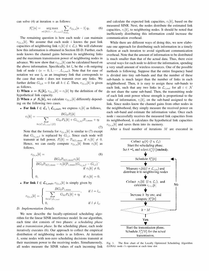
Fig. 1. The flow chart of the Locally Optimized Scheduling Algorithm(LOSA): node i’s operation at each time slot

the scheduling phase, the transmission phase begins. In thetransmission phase, each node i executes the decision Si[M ],i.e., the decision from the last iteration of the schedulingphase. Then, the actual link capacities at each time slot tare determined by the link capacities rl[M ] resulting fromthe decision Si[M ]’s, i.e., rl(t) = rl[M ]. Upon completingtransmission, each node updates the queue lengths of itsoutgoing links by

ql(t + 1) =

[ql(t) + κ

(U∑

u=1

Iul λu − rl(t)

)]+

, (9)

where κ is a constant step size and

Iul =

{1, if data of user u passes through link l,0, otherwise.

Recall that λu is the data rate of user u. After updating thequeues, each node moves to the next time slot t+1. The flowchart of the locally-optimized scheduling algorithm (LOSA)is shown in Fig. 1.

In our algorithm, each node collects queue lengths andlink capacities from its neighborhood, and carries out a fixednumber of computations regardless of the network size. Thus,the complexity of our algorithm depend on the size of theneighborhood and the number of iterations M , not on thenetwork size.

IV. EXTENSION TO THE LOGARITHMIC SINRINTERFERENCE MODEL

We now extend our algorithm to the logarithmic SINRinterference model. Recall that the main idea of our algorithmis that each node makes its own scheduling and power controldecision such that it is the best response (in terms of maxi-mizing the expected queue-weighted-link-capacity sum) underthe empirical distribution of neighboring nodes’ actions. InProposition 1, we showed that the best response for each nodeunder the linear SINR interference model is of the form that anode either schedules only one outgoing link with maximumpower, or schedules no link at all. The following proposition(Proposition 2) characterizes the condition on the best responsefor each node under the logarithmic SINR interference modelwhen the following assumption holds.

Assumption 1: For all nodes i and all links h, Gl1h = Gl2h

for all l1, l2 ∈ Li,out. In other words, the channel gain betweentwo links depends only on the transmitting node and thereceiving node.

Proposition 2: The optimal solution to (5) is given bythe solution to the following optimization problem whenAssumption 1 is satisfied:

max~p∈R

Li,out0

∑l∈Li

qlE[rl|~pi = ~p]

subject to ~1T ~p ≤ Pi,max

where RLi,out

0 is the set of Li,out-dimensional vectorssuch that at most one component is nonzero and theothers are zero, and the expectation is taken with respect

to the distribution of neighboring nodes’ scheduling decisions.

The detailed proof is provided in Appendix II. From Proposi-tion 2, given the distribution of neighboring nodes’ schedulingdecisions, the best response for each node i under the loga-rithmic SINR interference model is either to choose one linkto transmit or not to transmit at all. However, note that inProposition 2 the best response could be to transmit at anintermediate power level instead of always at full power as inProposition 1. Hence, we now need to take power control intoaccount. We define the decision vector of node i at time slott as,

~Di(t) , [Si(t), Pi(t)] (10)

for Si(t) ∈ {1, · · · , Li,out} and Pi(t) ∈ [0, Pi,max]. The deci-sion vector can be viewed as a generalization of the schedulingdecision in the previous section. The first component of thedecision vector, Si(t), denotes the scheduling decision of nodei as in Section III, and the second component, Pi(t), denotesthe transmission power of node i at time slot t. Therefore,~Di(t) = [s, p] corresponds the decision that node i schedulesthe s-th outgoing link with power p. Note that the case of‘scheduling no links’, i.e., ‘Si(t) = 0’, can be represented by‘Pi(t) = 0’.

We now extend the local optimization problem in (3) to thelogarithmic SINR interference model as follows,Extended Local Optimization: each node i searches its deci-sion vector ~Di = [s, p] that solves the following optimizationproblem,

maxs∈{1,··· ,Li,out}, p∈[0, Pi,max]

E

[∑l∈Li

rlql

∣∣∣∣ ~Di = [s, p]

], (11)

where the expectation is taken with respect to some empiricaldistribution of the other links’ decisions in Li. The extendedlocal optimization also has the following features similar to(3): each node updates only local queue lengths, maximizesonly the local queue-weighted-link-capacity sum, and choosesits own decision independently.

In order to find the optimal ~Di, we first find the locallyoptimal power assignment, P∗

i,s, for each scheduling decisions. Next, we find the scheduling decision S∗

i that maximizes(11). Specifically, each node i finds [P∗

i,1, P∗i,2, · · · , P∗

i,Li,out]

such that

P∗i,s = arg max

p∈[0, Pi,max]

∑l∈Li

qlE[rl

∣∣ ~Di = [s, p]], (12)

and then finds S∗i such that

S∗i = arg max

s∈{1,··· ,Li,out}

∑l∈Li

qlE[rl

∣∣ ~Di = [s, P∗i,s]]. (13)

The locally-optimal decision vector of node i can be repre-sented by ~D∗

i = [S∗i , P∗

i,S∗i].

To obtain ~D∗i , each node needs to estimate E[rl| ~Di =

[s, p]] for every link l in the neighborhood. We use the samemethod in Section III-C for estimating E[rl| ~Di = [s, p]] .We assume that neighboring nodes’ scheduling and power

control decisions follow the empirical distribution from thepast. Now consider the n-th iteration in a time slot. Let~Di[k] = [Si[k], Pi[k]] denote the decision vector of node i at apast iteration k. We also define the hypothetical link capacityunder the logarithmic SINR interference model as follows;rl|i,s,p[k] is the capacity of link l when the decision vectorof node i is [s, p] and the decision vectors of other nodes are~Dj [k] (j 6= i). Then, we can estimate E[rl| ~Di = [s, p]] atiteration n as an empirical average over the last W iterations,i.e.,

rl|i,s,p[n] ,1W

n−1∑k=n−W

rl|i,s,p[k]. (14)

However, maintaining rl|i,s,p[k] over all values of p in theinterval [0, Pi,max] is not realistic since the required memoryspace is too large. We now show that each node i canmaintain only rl|i,s,Pi,max [k] because the value of rl|i,s,p[k]for p < Pi,max can be derived easily from rl|i,s,Pi,max [k]. Tosee this, let ls be the s-th outgoing link of node i. Recall thatrl|i,s,Pi,max [k] is given by

rl|i,s,Pi,max [k] = (15)B log

(1 + GllPl[k]P

h∈Li\{l,ls} GhlPh[k]+GlslPi,max+ηl

),

if l 6= ls,

B log(1 + Glsls Pi,maxP

h∈Li\{l} GhlPh[k]+ηl

), if l = ls.

Note that the formula for rl|i,s,p[k] is similar to (15) exceptthat Pi,max is replaced by p. It is then easy to see that

rl|i,s,p[k] =

B log(

1 +al[k]

p + bl[k]

), if l 6= ls,

B log (1 + cl[k]p) , if l = ls,

where al[k] = GllPl[k]Glsl

, bl[k] = GllPl[k]/Glsl

exp(rl|i,s,Pi,max

[k]

B )−1− Pi,max,

and cl[k] = exp(rl|i,s,Pi,max

[k]

B )−1

Pi,max. Note that al[k], bl[k], and

cl[k] are readily obtainable because each node i is assumedto know the channel gains between its neighboring links andtheir transmission powers at each past iteration k.

Once each node can estimate rl|i,s,p[k], the power controlproblem (12) for each scheduling decision s at iteration n canbe rewritten with the hypothetical link capacities as follows;

P∗i,s[n] = arg max

p∈[0,Pi,max]

∑l∈Li

rl|i,s,p[n− 1]ql. (16)

The objective function of (16) is a continuous and differen-tiable function of p. Unfortunately, the function could havemultiple local maximizers in the domain [0, Pi,max]. Thus,to solve (16), we need to check all local maximizers inthe domain. Alternatively, we may approximate the solutionby simply searching among K points p1,...,pK where pk =(k−1)Pi,max

K−1 and takes the point pk that maximize (16) asan approximation of P∗

i,s[n]. Once the locally-optimal powerassignment P∗

i,s[n] is obtained for each scheduling decisions, we can find the locally optimal scheduling decision S∗

i [n]

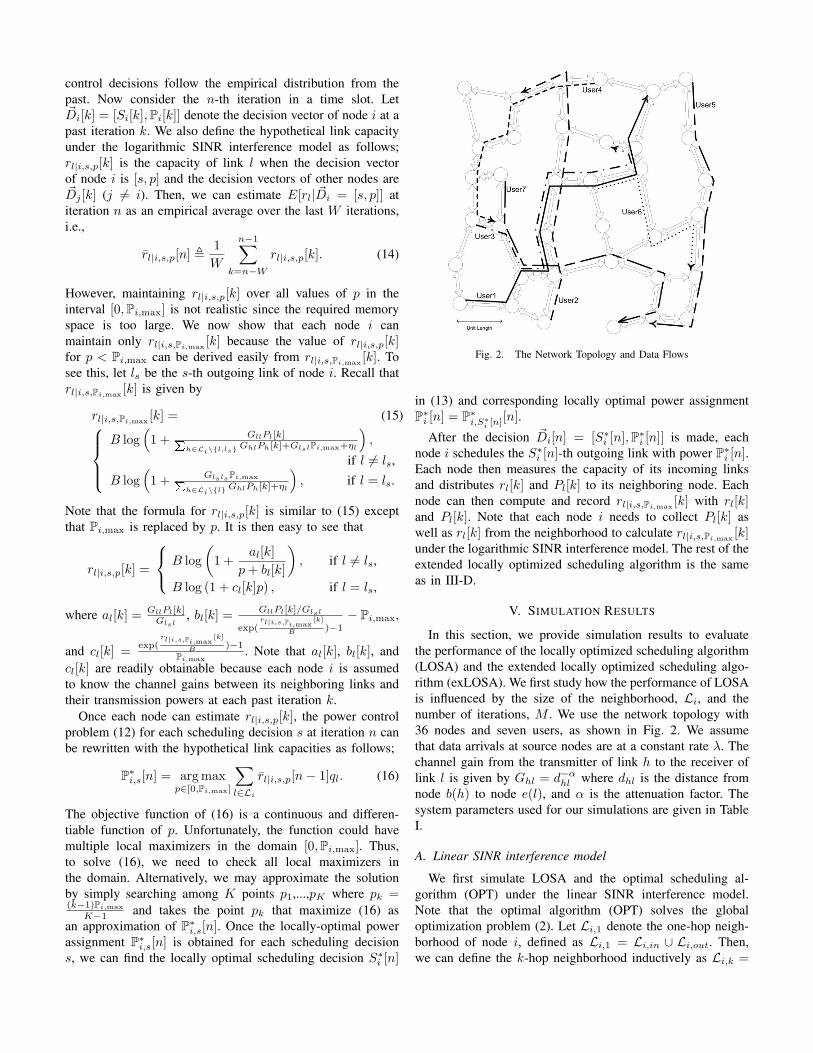
Fig. 2. The Network Topology and Data Flows

in (13) and corresponding locally optimal power assignmentP∗

i [n] = P∗i,S∗i [n][n].

After the decision ~Di[n] = [S∗i [n], P∗

i [n]] is made, eachnode i schedules the S∗

i [n]-th outgoing link with power P∗i [n].

Each node then measures the capacity of its incoming linksand distributes rl[k] and Pl[k] to its neighboring node. Eachnode can then compute and record rl|i,s,Pi,max [k] with rl[k]and Pl[k]. Note that each node i needs to collect Pl[k] aswell as rl[k] from the neighborhood to calculate rl|i,s,Pi,max [k]under the logarithmic SINR interference model. The rest of theextended locally optimized scheduling algorithm is the sameas in III-D.

V. SIMULATION RESULTS

In this section, we provide simulation results to evaluatethe performance of the locally optimized scheduling algorithm(LOSA) and the extended locally optimized scheduling algo-rithm (exLOSA). We first study how the performance of LOSAis influenced by the size of the neighborhood, Li, and thenumber of iterations, M . We use the network topology with36 nodes and seven users, as shown in Fig. 2. We assumethat data arrivals at source nodes are at a constant rate λ. Thechannel gain from the transmitter of link h to the receiver oflink l is given by Ghl = d−α

hl where dhl is the distance fromnode b(h) to node e(l), and α is the attenuation factor. Thesystem parameters used for our simulations are given in TableI.

A. Linear SINR interference model

We first simulate LOSA and the optimal scheduling al-gorithm (OPT) under the linear SINR interference model.Note that the optimal algorithm (OPT) solves the globaloptimization problem (2). Let Li,1 denote the one-hop neigh-borhood of node i, defined as Li,1 = Li,in ∪ Li,out. Then,we can define the k-hop neighborhood inductively as Li,k =

TABLE ISYSTEM PARAMETERS

Parameters ValuesBackground Noise (ηl) 0.1

Maximum Power (Pi,max) 1Attenuation Factor (α) 4

Bandwidth (B) 1Number of Past Records (W ) 5

Number of Time Slots 2000Step size (κ) 0.1Unit length 1

∪l∈Li,k−1(Lb(l),1 ∪ Le(l),1). In order to model practical con-straints that nodes cannot receive while it is transmitting, andnodes cannot receive from multiple transmitters simultane-ously, we set Ghl = ∞ if b(h) = e(l) or e(h) = e(l).

In Figs. 3(a) and 3(b), each curve illustrates the averagequeue length over all links for a given scheduling algorithm.Note that the scheduling algorithms that result in curves tothe right can carry a larger load and therefore have betterperformance.

Fig. 3(a) shows the relationship between the size of neigh-borhood and performance. Each curve labeled with ‘LOSA’corresponds to the results from LOSA where Li consistsof links in each k-hop neighborhood (i.e., Li , Li,k) fork = 1, 2, 3, respectively. In this simulation, we set thenumber of iterations in each time slot M = 30. From thesimulation result, we can see that the algorithm using the largerneighborhood has a larger throughput.

Next, Fig. 3(b) shows the relationship between the numberof iterations and performance. Each curve labeled with ‘LOSA’corresponds to the results from LOSA where the total numberof iterations is M = 10, 20, 30, respectively. We choose Li ,Li,3 in this simulation. From the figure, we can observe thatall values of M results into a throughput that is reasonablyclose to the optimal.

B. Logarithmic SINR interference model

We now compare the performance of exLOSA to that ofthe other algorithms developed under the logarithmic SINRinterference model. For this comparison, we select the fol-lowing two scheduling and power control algorithms fromthe literature: JOCP algorithm [11] and a distributed ap-proximation algorithm , approx-DRPC, to the optimal DRPCalgorithm in [3]. JOCP in [11] solves the global optimizationproblem (2) under the assumption that the SINR values of alllinks are high, i.e., rl(t) = B log(1 + ξl(t)) ≈ B log(ξl(t)).Note that this high-SINR assumption excludes the need forscheduling in JOCP. Hence, the solution for JOCP will forceall links to be active simultaneously at some optimized powerlevels. In [3], after developing the optimal DRPC algorithm(which is centralized with high computational complexity),the authors also proposed a distributed heuristic algorithm forapproximating DRPC, where each node randomly decides tobe a transmitter with a given probability and then decide whichnode it should transmit to using the feedback from adjacentreceiving nodes. Finally, in order to study the improvement dueto the power control capability of exLOSA, we also simulate

(a) Different k-hop neighborhood

(b) Different number of iterations M

Fig. 3. The average queue length under the linear SINR interference modelas we vary (a) the size of neighborhood with M = 30 and (b) the numberof iterations with k = 3

LOSA under the logarithmic SINR interference model. In therest of our simulations, we set M = 30 and Li , Li,3.

We first compare the performance of these algorithms underthe same physical constraint, i.e., Ghl = ∞ if b(h) = e(l) ore(h) = e(l). Fig. 4 shows the average queue length of thesealgorithms at different loads λ. From Fig. 4, we can see thatexLOSA performs significantly better than JOCP and approx-DRPC. The performance improvement over approx-DRPC isexpected because our algorithm uses a more sophisticatedprocedure to choose transmission patterns than approx-DRPC.The performance improvement over JOCP is because JOCPis developed under the high-SINR assumption, which is oftenviolated in practice. There are two reasons why the high-SINRassumption may be violated. The first is that an outgoinglink from a node can create excessive self-interference tothe incoming links. Since in JOCP the optimal solution isto operate all links simultaneously, this self-interference willlead to low-SINR values. To verify this, we intentionallymodify the simulation setting such that the nodes are ableto receive from multiple transmitters and to receive while

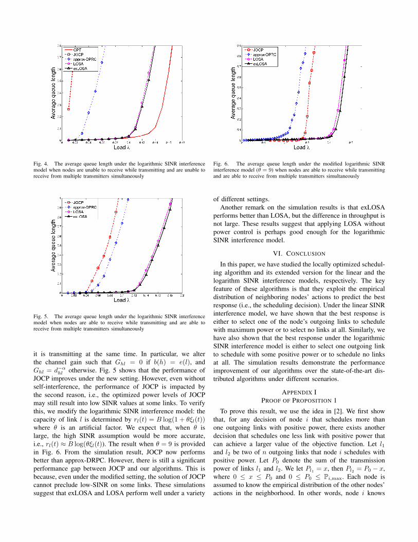
Fig. 4. The average queue length under the logarithmic SINR interferencemodel when nodes are unable to receive while transmitting and are unable toreceive from multiple transmitters simultaneously

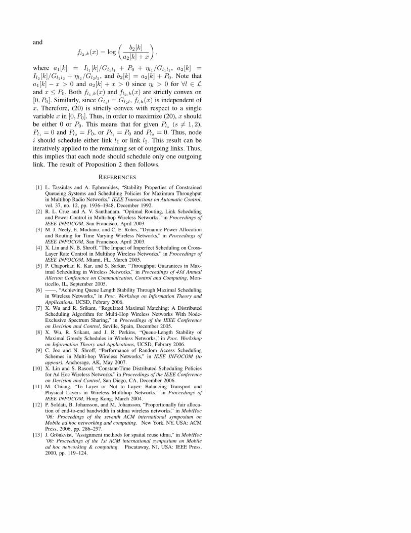
Fig. 5. The average queue length under the logarithmic SINR interferencemodel when nodes are able to receive while transmitting and are able toreceive from multiple transmitters simultaneously

it is transmitting at the same time. In particular, we alterthe channel gain such that Ghl = 0 if b(h) = e(l), andGhl = d−α

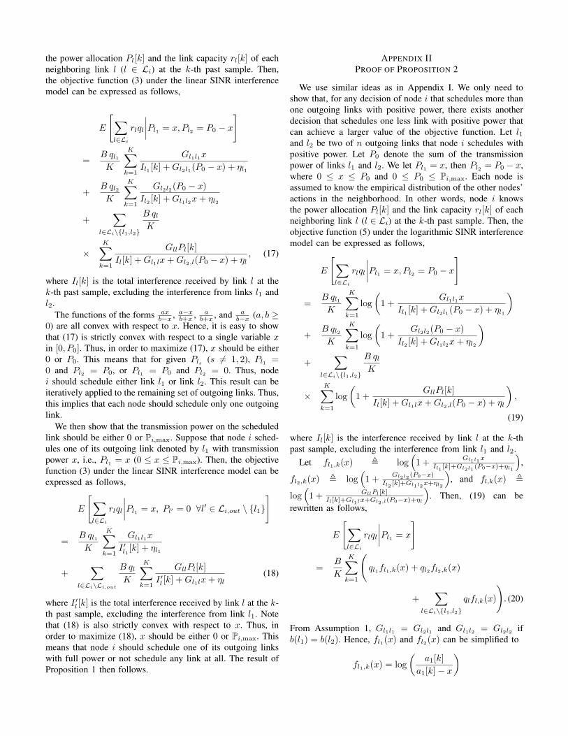
hl otherwise. Fig. 5 shows that the performance ofJOCP improves under the new setting. However, even withoutself-interference, the performance of JOCP is impacted bythe second reason, i.e., the optimized power levels of JOCPmay still result into low SINR values at some links. To verifythis, we modify the logarithmic SINR interference model: thecapacity of link l is determined by rl(t) = B log(1 + θξl(t))where θ is an artificial factor. We expect that, when θ islarge, the high SINR assumption would be more accurate,i.e., rl(t) ≈ B log(θξl(t)). The result when θ = 9 is providedin Fig. 6. From the simulation result, JOCP now performsbetter than approx-DRPC. However, there is still a significantperformance gap between JOCP and our algorithms. This isbecause, even under the modified setting, the solution of JOCPcannot preclude low-SINR on some links. These simulationssuggest that exLOSA and LOSA perform well under a variety

Fig. 6. The average queue length under the modified logarithmic SINRinterference model (θ = 9) when nodes are able to receive while transmittingand are able to receive from multiple transmitters simultaneously

of different settings.Another remark on the simulation results is that exLOSA

performs better than LOSA, but the difference in throughput isnot large. These results suggest that applying LOSA withoutpower control is perhaps good enough for the logarithmicSINR interference model.

VI. CONCLUSION

In this paper, we have studied the locally optimized schedul-ing algorithm and its extended version for the linear and thelogarithm SINR interference models, respectively. The keyfeature of these algorithms is that they exploit the empiricaldistribution of neighboring nodes’ actions to predict the bestresponse (i.e., the scheduling decision). Under the linear SINRinterference model, we have shown that the best response iseither to select one of the node’s outgoing links to schedulewith maximum power or to select no links at all. Similarly, wehave also shown that the best response under the logarithmicSINR interference model is either to select one outgoing linkto schedule with some positive power or to schedule no linksat all. The simulation results demonstrate the performanceimprovement of our algorithms over the state-of-the-art dis-tributed algorithms under different scenarios.

APPENDIX IPROOF OF PROPOSITION 1

To prove this result, we use the idea in [2]. We first showthat, for any decision of node i that schedules more thanone outgoing links with positive power, there exists anotherdecision that schedules one less link with positive power thatcan achieve a larger value of the objective function. Let l1and l2 be two of n outgoing links that node i schedules withpositive power. Let P0 denote the sum of the transmissionpower of links l1 and l2. We let Pl1 = x, then Pl2 = P0 − x,where 0 ≤ x ≤ P0 and 0 ≤ P0 ≤ Pi,max. Each node isassumed to know the empirical distribution of the other nodes’actions in the neighborhood. In other words, node i knows

the power allocation Pl[k] and the link capacity rl[k] of eachneighboring link l (l ∈ Li) at the k-th past sample. Then,the objective function (3) under the linear SINR interferencemodel can be expressed as follows,

E

[∑l∈Li

rlql

∣∣∣∣Pl1 = x, Pl2 = P0 − x

]

=B ql1

K

K∑k=1

Gl1l1x

Il1 [k] + Gl2l1(P0 − x) + ηl1

+B ql2

K

K∑k=1

Gl2l2(P0 − x)Il2 [k] + Gl1l2x + ηl2

+∑

l∈Li\{l1,l2}

B ql

K

×K∑

k=1

GllPl[k]Il[k] + Gl1lx + Gl2,l(P0 − x) + ηl

, (17)

where Il[k] is the total interference received by link l at thek-th past sample, excluding the interference from links l1 andl2.

The functions of the forms axb−x , a−x

b+x , ab+x , and a

b−x (a, b ≥0) are all convex with respect to x. Hence, it is easy to showthat (17) is strictly convex with respect to a single variable xin [0, P0]. Thus, in order to maximize (17), x should be either0 or P0. This means that for given Pls (s 6= 1, 2), Pl1 =0 and Pl2 = P0, or Pl1 = P0 and Pl2 = 0. Thus, nodei should schedule either link l1 or link l2. This result can beiteratively applied to the remaining set of outgoing links. Thus,this implies that each node should schedule only one outgoinglink.

We then show that the transmission power on the scheduledlink should be either 0 or Pi,max. Suppose that node i sched-ules one of its outgoing link denoted by l1 with transmissionpower x, i.e., Pl1 = x (0 ≤ x ≤ Pi,max). Then, the objectivefunction (3) under the linear SINR interference model can beexpressed as follows,

E

[∑l∈Li

rlql

∣∣∣∣Pl1 = x, Pl′ = 0 ∀l′ ∈ Li,out \ {l1}

]

=B ql1

K

K∑k=1

Gl1l1x

I ′l1 [k] + ηl1

+∑

l∈Li\Li,out

B ql

K

K∑k=1

GllPl[k]I ′l [k] + Gl1lx + ηl

(18)

where I ′l [k] is the total interference received by link l at the k-th past sample, excluding the interference from link l1. Notethat (18) is also strictly convex with respect to x. Thus, inorder to maximize (18), x should be either 0 or Pi,max. Thismeans that node i should schedule one of its outgoing linkswith full power or not schedule any link at all. The result ofProposition 1 then follows.

APPENDIX IIPROOF OF PROPOSITION 2

We use similar ideas as in Appendix I. We only need toshow that, for any decision of node i that schedules more thanone outgoing links with positive power, there exists anotherdecision that schedules one less link with positive power thatcan achieve a larger value of the objective function. Let l1and l2 be two of n outgoing links that node i schedules withpositive power. Let P0 denote the sum of the transmissionpower of links l1 and l2. We let Pl1 = x, then Pl2 = P0 − x,where 0 ≤ x ≤ P0 and 0 ≤ P0 ≤ Pi,max. Each node isassumed to know the empirical distribution of the other nodes’actions in the neighborhood. In other words, node i knowsthe power allocation Pl[k] and the link capacity rl[k] of eachneighboring link l (l ∈ Li) at the k-th past sample. Then, theobjective function (5) under the logarithmic SINR interferencemodel can be expressed as follows,

E

[∑l∈Li

rlql

∣∣∣∣Pl1 = x, Pl2 = P0 − x

]

=B ql1

K

K∑k=1

log(

1 +Gl1l1x

Il1 [k] + Gl2l1(P0 − x) + ηl1

)

+B ql2

K

K∑k=1

log(

1 +Gl2l2(P0 − x)

Il2 [k] + Gl1l2x + ηl2

)+

∑l∈Li\{l1,l2}

B ql

K

×K∑

k=1

log(

1 +GllPl[k]

Il[k] + Gl1lx + Gl2,l(P0 − x) + ηl

),

(19)

where Il[k] is the interference received by link l at the k-thpast sample, excluding the interference from link l1 and l2.

Let fl1,k(x) , log(1 + Gl1l1x

Il1 [k]+Gl2l1 (P0−x)+ηl1

),

fl2,k(x) , log(1 + Gl2l2 (P0−x)

Il2 [k]+Gl1l2x+ηl2

), and fl,k(x) ,

log(1 + GllPl[k]

Il[k]+Gl1lx+Gl2,l(P0−x)+ηl

). Then, (19) can be

rewritten as follows,

E

[∑l∈Li

rlql

∣∣∣∣Pl1 = x

]

=B

K

K∑k=1

(ql1fl1,k(x) + ql2fl2,k(x)

+∑

l∈Li\{l1,l2}

qlfl,k(x)

). (20)

From Assumption 1, Gl1l1 = Gl2l1 and Gl1l2 = Gl2l2 ifb(l1) = b(l2). Hence, fl1(x) and fl2(x) can be simplified to

fl1,k(x) = log(

a1[k]a1[k]− x

)

andfl2,k(x) = log

(b2[k]

a2[k] + x

),

where a1[k] = Il1 [k]/Gl1l1 + P0 + ηl1/Gl1l1 , a2[k] =Il2 [k]/Gl2l2 + ηl2/Gl2l2 , and b2[k] = a2[k] + P0. Note thata1[k] − x > 0 and a2[k] + x > 0 since ηl > 0 for ∀l ∈ Land x ≤ P0. Both fl1,k(x) and fl2,k(x) are strictly convex on[0, P0]. Similarly, since Gl1l = Gl2l, fl,k(x) is independent ofx. Therefore, (20) is strictly convex with respect to a singlevariable x in [0, P0]. Thus, in order to maximize (20), x shouldbe either 0 or P0. This means that for given Pls (s 6= 1, 2),Pl1 = 0 and Pl2 = P0, or Pl1 = P0 and Pl2 = 0. Thus, nodei should schedule either link l1 or link l2. This result can beiteratively applied to the remaining set of outgoing links. Thus,this implies that each node should schedule only one outgoinglink. The result of Proposition 2 then follows.

REFERENCES

[1] L. Tassiulas and A. Ephremides, “Stability Properties of ConstrainedQueueing Systems and Scheduling Policies for Maximum Throughputin Multihop Radio Networks,” IEEE Transactions on Automatic Control,vol. 37, no. 12, pp. 1936–1948, December 1992.

[2] R. L. Cruz and A. V. Santhanam, “Optimal Routing, Link Schedulingand Power Control in Multi-hop Wireless Networks,” in Proceedings ofIEEE INFOCOM, San Francisco, April 2003.

[3] M. J. Neely, E. Modiano, and C. E. Rohrs, “Dynamic Power Allocationand Routing for Time Varying Wireless Networks,” in Proceedings ofIEEE INFOCOM, San Francisco, April 2003.

[4] X. Lin and N. B. Shroff, “The Impact of Imperfect Scheduling on Cross-Layer Rate Control in Multihop Wireless Networks,” in Proceedings ofIEEE INFOCOM, Miami, FL, March 2005.

[5] P. Chaporkar, K. Kar, and S. Sarkar, “Throughput Guarantees in Max-imal Scheduling in Wireless Networks,” in Proceedings of 43d AnnualAllerton Conference on Communication, Control and Computing, Mon-ticello, IL, September 2005.

[6] ——, “Achieving Queue Length Stability Through Maximal Schedulingin Wireless Networks,” in Proc. Workshop on Information Theory andApplications, UCSD, Febrary 2006.

[7] X. Wu and R. Srikant, “Regulated Maximal Matching: A DistributedScheduling Algorithm for Multi-Hop Wireless Networks With Node-Exclusive Spectrum Sharing,” in Proceedings of the IEEE Conferenceon Decision and Control, Seville, Spain, December 2005.

[8] X. Wu, R. Srikant, and J. R. Perkins, “Queue-Length Stability ofMaximal Greedy Schedules in Wireless Networks,” in Proc. Workshopon Information Theory and Applications, UCSD, Febrary 2006.

[9] C. Joo and N. Shroff, “Performance of Random Access SchedulingSchemes in Multi-hop Wireless Networks,” in IEEE INFOCOM (toappear), Anchorage, AK, May 2007.

[10] X. Lin and S. Rasool, “Constant-Time Distributed Scheduling Policiesfor Ad Hoc Wireless Networks,” in Proceedings of the IEEE Conferenceon Decision and Control, San Diego, CA, December 2006.

[11] M. Chiang, “To Layer or Not to Layer: Balancing Transport andPhysical Layers in Wireless Multihop Networks,” in Proceedings ofIEEE INFOCOM, Hong Kong, March 2004.

[12] P. Soldati, B. Johansson, and M. Johansson, “Proportionally fair alloca-tion of end-to-end bandwidth in stdma wireless networks,” in MobiHoc’06: Proceedings of the seventh ACM international symposium onMobile ad hoc networking and computing. New York, NY, USA: ACMPress, 2006, pp. 286–297.

[13] J. Gronkvist, “Assignment methods for spatial reuse tdma,” in MobiHoc’00: Proceedings of the 1st ACM international symposium on Mobilead hoc networking & computing. Piscataway, NJ, USA: IEEE Press,2000, pp. 119–124.