Enhancing self-scheduling algorithms via synchronization and weighting (PLEASE REFERENCE IN YOUR...

J. Parallel Distrib. Comput. 68 (2008) 246–264www.elsevier.com/locate/jpdc

Enhancing self-scheduling algorithms via synchronization and weighting

Florina M. Ciorbaa,∗, Ioannis Riakiotakisa, Theodore Andronikosb, George Papakonstantinoua,Anthony T. Chronopoulosc

aComputing Systems Laboratory, Department of Electrical and Computer Engineering, National Technical University of Athens, Zografou Campus, 15773Athens, Greece

bDepartment of Informatics, Ionian University, 7, Tsirigoti Square, 49100 Corfu, GreececDepartment of Computer Science, University of Texas at San Antonio, 6900 N. Loop 1604 West, San Antonio, TX 78249, USA

Received 2 June 2006; received in revised form 9 January 2007; accepted 12 July 2007Available online 8 August 2007

Abstract

Existing dynamic self-scheduling algorithms, used to schedule independent tasks on heterogeneous clusters, cannot handle tasks withdependencies because they lack the support for internode communication. To compensate for this deficiency we introduce a synchronizationmechanism that provides inter-processor communication, thus, enabling self-scheduling algorithms to handle efficiently nested loops withdependencies. We also present a weighting mechanism that significantly improves the performance of dynamic self-scheduling algorithms.These algorithms divide the total number of tasks into chunks and assign them to processors. The weighting mechanism adapts the chunksizes to the computing power and current run-queue state of the processors. The synchronization and weighting mechanisms are orthogonal,in the sense that they can simultaneously be applied to loops with dependencies. Thus, they broaden the application spectrum of dynamicself-scheduling algorithms and improve their performance. Extensive testing confirms the efficiency of the synchronization and weightingmechanisms and the significant improvement of the synchronized–weighted versions of the algorithms over the synchronized-only versions.© 2007 Elsevier Inc. All rights reserved.

Keywords: Dynamic load balancing algorithms; Loops with dependencies; Synchronization; Weighting; Non-dedicated heterogeneous systems

1. Introduction

Many scheduling algorithms were devised in the past fewyears for general distributed systems, composed of non-identical processing nodes, called heterogeneous distributedsystems. Load balancing is one of the most challenging issuesin attaining high performance in heterogenous distributed sys-tems. In this article we deal with two important cases of theload balancing problem when running loops with and withoutdependencies. We consider: (1) loops with tasks of uneven sizeand (2) loops executed on non-dedicated distributed systems.Load balancing is usually achieved by relocating applicationtasks from busy nodes to lightly loaded or idle nodes [8]. Someload balancing algorithms for homogeneous systems werepresented in [2,16], and for heterogeneous systems in [11,24].

∗ Corresponding author. Fax: +30 2107721533.E-mail address: [email protected] (F.M. Ciorba).

0743-7315/$ - see front matter © 2007 Elsevier Inc. All rights reserved.doi:10.1016/j.jpdc.2007.07.003

Another categorization of scheduling algorithms for dis-tributed systems is static versus dynamic. A review of classicstatic algorithms for task graphs is given in [15]. Static schedul-ing algorithms [1,22] are not effective for non-dedicated dis-tributed systems. One reason is that the workload distributionof many applications cannot be predicted. Also the availablecomputation power of the processing node may not be knownin advance or may not remain constant throughout the appli-cation’s execution. Dynamic algorithms [10] strive to achieveload balancing under load variation. The performance of dy-namic load balancing algorithms in practice is determined bytheir ability to adapt to a dynamic and, in most cases, unpre-dictable environment. They use runtime state information ofthe system in order to make informative decisions on balancingthe workload. This makes them applicable to a much largerspectrum of applications. In [8] different dynamic load balanc-ing algorithms with different complexities were compared.

Many important applications involve loops with or withoutdependencies among their iterations. An important class of

http://www.elsevier.com/locate/jpdc

mailto:[email protected]

F.M. Ciorba et al. / J. Parallel Distrib. Comput. 68 (2008) 246–264 247

dynamic scheduling algorithms are the self-schedulingschemes: chunk self-scheduling (CSS) [14], guided self-scheduling (GSS) [21], trapezoid self-scheduling (TSS) [23],factoring self-scheduling (FSS) [13]. These algorithms weredevised for nested loops without dependencies executed onhomogenous systems. Self-scheduling algorithms divide thetotal number of tasks into chunks, which are then assigned toprocessors (slaves). In their original form, these algorithmsdo not perform satisfactorily on non-dedicated heterogeneoussystems and cannot handle loops with dependencies. A firstattempt to make self-scheduling algorithms suitable for het-erogeneous systems was weighted factoring (WF) that wasproposed in [12]. WF differs from FSS in that the chunkssizes are weighted according to the processing powers ofthe slaves. However, in WF the processor weights remainconstant throughout the parallel execution. Banicescu et al.proposed in [4] a method called adaptive weighted factoring(AWF) that adjusts the processor weights according to tim-ing information reflecting variations of slaves computationpower. This was designed for time-stepping scientific applica-tions. Chronopoulos et al. extended in [5] the TSS algorithm,proposing the distributed TSS (DTSS) algorithm suitable fordistributed systems. In DTSS the chunks sizes are weighted bythe slaves relative power and the number of processes in theirrun-queue.

However, in spite of these developments, self-schedulingalgorithms were still not applicable to loops with dependen-cies. To the best of our knowledge, the first work that ap-plied self-scheduling algorithms to dependence loops was [7].Therein, CSS, TSS and DTSS were enhanced via synchroniza-tion points (SPs) so as to enable inter-slave communication andto satisfy the loop dependencies. Loop unrolling for enhanc-ing parallelization of loops with dependencies has been stud-ied in [20] and references therein. However, loop unrolling isnot practical for a large number of iterations because the un-rolling factor depends on the size of the available registers.Moreover, it is not easy to determine the unrolling factor inadvance.

In this paper we extend and generalize the work in [7] byconstructing a general synchronization mechanism S, which ap-plies to all loop self-scheduling schemes. When this mechanismis applied to a self-scheduling algorithm, it enables it to han-dle efficiently loops with dependencies. The synchronizationmechanism S inserts SPs in the execution flow so that slavesperform the appropriate data exchanges. This mechanism is notincorporated within the self-scheduling algorithm, but it is anadditional stand-alone component, applicable without furthermodifications. Given a self-scheduling algorithm A, its syn-chronized version is denoted S-A. By enabling self-schedulingalgorithms to be applicable to loops with dependencies, whichwas not the case before, the spectrum of applications isextended.

In addition, motivated by the results in [3,5,12], we de-fine a weighting mechanism W , aimed at improving the loadbalancing and, thus, the performance of all non-adaptiveself-scheduling algorithms on non-dedicated heterogeneoussystems. This mechanism is inspired from the approach used in

[5], i.e., it uses the relative powers of the slaves combined withinformation regarding their run-queues to compute chunks.However, in contrast to previous approaches to chunk weight-ing, this mechanism is not embedded within the self-schedulingalgorithm, but it is an external stand-alone component appli-cable to any dynamic algorithm without modifications. Givenany self-scheduling algorithm A, its weighted version will becalled W-A.

Self-scheduling algorithms were usually implemented on dis-tributed memory systems using the master–slave model. In thismodel, communication takes place only between the master andthe slaves. The existence of dependencies necessitates commu-nication among slaves, making the standard master-slave modelinadequate. Therefore, an extended version of the master–slavemodel is required in the synchronized version of the self-scheduling algorithms. In the extended model communicationamong slaves is performed by direct data exchanges from slaveto slave, and not through the master. In this approach, the mas-ter has a global view of the system’s load and decides uponallocating the tasks to each slave.

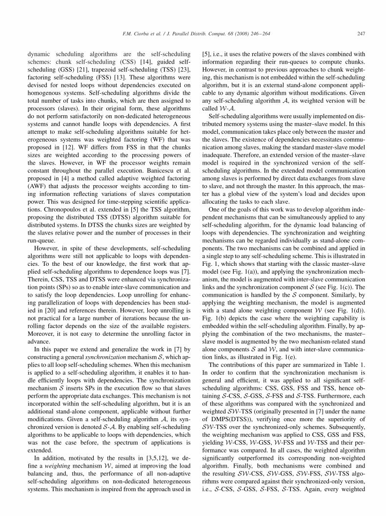
One of the goals of this work was to develop algorithm inde-pendent mechanisms that can be simultaneously applied to anyself-scheduling algorithm, for the dynamic load balancing ofloops with dependencies. The synchronization and weightingmechanisms can be regarded individually as stand-alone com-ponents. The two mechanisms can be combined and applied ina single step to any self-scheduling scheme. This is illustrated inFig. 1, which shows that starting with the classic master–slavemodel (see Fig. 1(a)), and applying the synchronization mech-anism, the model is augmented with inter-slave communicationlinks and the synchronization component S (see Fig. 1(c)). Thecommunication is handled by the S component. Similarly, byapplying the weighting mechanism, the model is augmentedwith a stand alone weighting component W (see Fig. 1(d)).Fig. 1(b) depicts the case where the weighting capability isembedded within the self-scheduling algorithm. Finally, by ap-plying the combination of the two mechanisms, the master–slave model is augmented by the two mechanism-related standalone components S and W , and with inter-slave communica-tion links, as illustrated in Fig. 1(e).

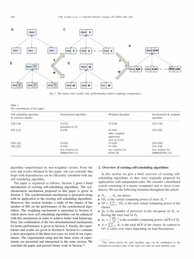
The contributions of this paper are summarized in Table 1.In order to confirm that the synchronization mechanism isgeneral and efficient, it was applied to all significant self-scheduling algorithms: CSS, GSS, FSS and TSS, hence ob-taining S-CSS, S-GSS, S-FSS and S-TSS. Furthermore, eachof these algorithms was compared with the synchronized andweighted SW-TSS (originally presented in [7] under the nameof DMPS(DTSS)), verifying once more the superiority ofSW-TSS over the synchronized-only schemes. Subsequently,the weighting mechanism was applied to CSS, GSS and FSS,yielding W-CSS, W-GSS, W-FSS and W-TSS and their per-formance was compared. In all cases, the weighted algorithmsignificantly outperformed its corresponding non-weightedalgorithm. Finally, both mechanisms were combined andthe resulting SW-CSS, SW-GSS, SW-FSS, SW-TSS algo-rithms were compared against their synchronized-only version,i.e., S-CSS, S-GSS, S-FSS, S-TSS. Again, every weighted

248 F.M. Ciorba et al. / J. Parallel Distrib. Comput. 68 (2008) 246–264

Master

Slave Slave Slave

Master

Slave W Slave W Slave W

Master

Slave

S

Slave SlaveS S S

Master

Slave

W

Slave SlaveW W W

Master

Slave Slave Slave

S W

SW S W SW

S

W W

S

W

a

b

c

d

e

Fig. 1. The master–slave model with synchronization and/or weighting component(s).

Table 1The contributions of this paper

Self-scheduling algorithm Synchronized algorithm Weighted algorithm Synchronized & weighted& reference number algorithm

CSS [14] S-CSS W-CSS SW-CSSpresented in [7]

FSS [13] S-FSS W-FSS SW-FSSother weightedapproachesexist in [3,12]

GSS [21] S-GSS W-GSS SW-GSSTSS [23] S-TSS W-TSS SW-TSS

new notation for new notation for new notation forDMPS(TSS) [7] DTSS [5] DMPS(DTSS) [7]

algorithm outperformed its non-weighted version. From thetests and results obtained in this paper, one can conclude thatloops with dependencies can be efficiently scheduled with anyself-scheduling algorithm.

The paper is organized as follows. Section 2 gives a briefintroduction of existing self-scheduling algorithms. The syn-chronization mechanism proposed in this paper is given inSection 3. The synchronization mechanism is presented alongwith its application to the existing self-scheduling algorithms.Moreover, this section includes a study of the impact of thenumber of SPs on the performance of the synchronized algo-rithms. The weighting mechanism is presented in Section 4,which shows how self-scheduling algorithms can be enhancedwith this mechanism in order to achieve better load balancing.Next, the combination of the two aforementioned mechanismsfor better performance is given in Section 5. Finally, the exper-iments and results are given in Section 6. Section 6.1 containsa short description of the three test cases we used in our exper-iments. The experimental setup and the three series of exper-iments are presented and interpreted in the same section. Weconclude the paper and present future work in Section 7.

2. Overview of existing self-scheduling algorithms

In this section we give a brief overview of existing self-scheduling algorithms, as they were originally proposed forapplications with independent tasks. We consider a distributedsystem consisting of a master (computer) and m slaves (com-puters). We use the following notations throughout this article:

• P1, . . . , Pm are slaves.• VPk is the virtual computing power of slave Pk . 1

• VP = ∑mk=1 VPk is the total virtual computing power of the

cluster.• Qk is the number of processes in the run-queue of Pk , re-

flecting the total load of Pk .

• Ak =⌊

VPk

Qk

⌋is the available computing power (ACP) of Pk .

• A = ∑mk=1 Ak is the total ACP of the cluster. In contrast to

VP, A varies over times depending on load fluctuations.

1 The virtual power for each machine type can be established as thenormalized execution time of the same test suite on each machine type.


• N is the number of scheduling steps, i = 1, . . . , N , for agiven algorithm.

• A few consecutive iterations of the loop are called a chunk;Ci is the chunk size at the ith scheduling step.

A nested loop is modeled as an n-dimensional Cartesian spaceJ (J ⊂ Zn), called index space, where n is the depth of theloop nest. Each point of this n-dimensional index space is adistinct iteration of the loop body. Without loss of generalitywe assume that for every index point (u1, . . . , un) it holds that1�ui �Ui , 1� i�n.

We can now give an overview of the following self-scheduling schemes: CSS, GSS, FSS, TSS and DTSS, wherewe assume that the master–slave model is used and the slavesare assigned the iterations to be executed by the master.

CSS [14] assigns constant size chunks to each slave, i.e.,Ci = constant . The chunk size is chosen by the user. If Ci =1 then CSS is the so-called (pure) self-scheduling. A largechunk size reduces scheduling overhead, but also increases thechance of load imbalance, due to the difficulty to predict anoptimal chunk size. As a compromise between load imbalanceand scheduling overhead, other schemes start with large chunksizes in order to reduce the scheduling overhead and reduce thechunk sizes throughout the execution to improve load balanc-ing. These schemes are known as reducing chunk size algo-rithms and their difference lies in the choice of the first chunkand the computation of the decrement.

In the GSS [21] scheme, each slave is assigned a chunkgiven by the number of remaining iterations divided by thenumber of slaves, i.e., Ci = Ri/m, where Ri is the number ofremaining iterations. Assuming that the loop which is sched-uled with GSS is the r-th loop, where 1�r �n, then R0 isthe total number of iterations, i.e., |Ur |, and Ri+1 = Ri − Ci ,

where Ci = �Ri/m� =⌈(

1 − 1m

)i · |Ur |m

⌉. This scheme ini-

tially assigns large chunks, which implies reduced communi-cation/scheduling overheads in the beginning. At the last stepssmall chunks are assigned to improve the load balancing, at theexpense of increased communication/scheduling overhead.

The TSS [23] scheme linearly decreases the chunk size Ci .The first and last (assigned) chunk size pair (F, L) may be setby the programmer. A conservative selection for the (F, L) pair

is: F = |Ur |2∗m

and L = 1, where m is the number of slaves.This ensures that the load of the first chunk is less than 1/m ofthe total load in most loop distributions and reduces the chanceof imbalance due to a large first chunk. Still many synchro-nizations may occur. One can improve this by choosing L >

1. The proposed number of steps needed for the scheduling

process is N = 2×|Ur |(F+L)

. Thus, the decrement between consec-

utive chunks is D = (F − L)/(N − 1), and the chunk sizesare C1 = F, C2 = F − D, C3 = F − 2 × D, . . . , CN =F − (N − 1) × D. TSS improves GSS for loops with varyingtasks sizes, as it is explained in detail in [18].

The FSS [3] scheme schedules iterations in batches of m

equal chunks. In each batch, a slave is assigned a chunk sizegiven by a subset of the remaining iterations (usually half)divided by the number of slaves. The chunk size in this case is

Ci =⌈

Ri

�∗m

⌉and Ri+1 = Ri −(m×Ci), where the parameter �

is computed (by a probability distribution) or is sub-optimallychosen � = 2. The weakness of this scheme is the difficultyto determine the optimal parameters. However, tests show [3]improvement on previous adaptive schemes (possibly) due tofewer adaptations of the chunk-size.

DTSS [5,6] improves on TSS by selecting the chunk sizesaccording to the computational power of the slaves. DTSS usesa model that includes the number of processes in the run-queueof each slave. Every process running on a slave is assumed totake an equal share of its computing resources. The applica-tion programmer may determine the pair (F, L) according toTSS, or the following formula may be used in the conserva-tive selection approach: F = |Ur |

2×Aand L = 1 (assuming that

the loop which is scheduled by DTSS is the r-th loop). The

total number of steps is N = 2×|Ur |(F+L)

and the chunk decrementis D = (F − L)/(N − 1). The size of a chunk in this case isCi = Ak × (F − D × (Sk−1 + (Ak − 1)/2)), where: Sk−1 =A1 +· · ·+Ak−1. When all slaves are dedicated to a single userjob then Ak = VPk . Also, when all slaves have the same speed,then VPk = 1 and the tasks assigned in DTSS are the same as inTSS. The important difference between DTSS and TSS is thatin DTSS the next chunk is allocated according to the slave’sACP. Hence, faster slaves get more loop iterations than slowerones. In contrast, TSS simply treats all slaves in the same way.

3. The synchronization mechanism

The self-scheduling schemes described in the previous sec-tion are applicable to loops without dependencies. Nested loops,however, fall in two categories: parallel and dependence loops.Parallel loops have no dependencies among iterations and, thus,their iterations can be executed in any order or even simultane-ously. In dependence loops the iterations depend on each other,hence, imposing a certain execution order, according to the ex-isting dependencies. The loop body may contain general pro-gram statements that include if blocks and other for or whileloops. We assume that the nested loop has p uniform depen-dencies. These are modeled by dependence vectors and theirset is denoted DS = {�d1, . . . , �dp}.

The purpose of the synchronization mechanism is to enableself-scheduling algorithms to handle loops with dependencies.Recall that self-scheduling algorithms are devised for parallelloops and as such do not provide inter-slave communication.In [7] it was shown that CSS, TSS and DTSS can be appliedto dependence loops by SPs to compensate for this deficiency.In this paper we generalize this approach and define a syn-chronization mechanism applicable to all self-scheduling algo-rithms. In all cases the master assigns chunks to slaves whichsynchronize with each other at SPs. We must emphasize thatthe synchronization mechanism is completely independent ofthe self-scheduling algorithm and does not enhance the loadbalancing capability of the algorithm. Therefore, synchronizedself-scheduling algorithms perform well on heterogeneous sys-tems only if the self-scheduling algorithm itself explicitly takesinto account the heterogeneity. The synchronization overhead


Synchronization dimension

Ch

un

k/S

ch

ed

ulin

g d

ime

nsio

n

SISI SI

SP1 SPj-1 SPj SP#SPs

Vi+1

Vi-1

Vi

uc

us

current

slave

previous

slave

Uc

UsSI SI

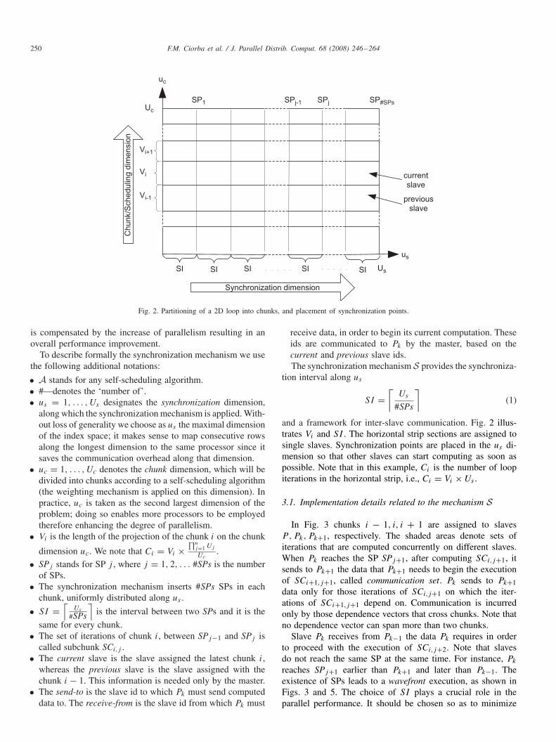
Fig. 2. Partitioning of a 2D loop into chunks, and placement of synchronization points.

is compensated by the increase of parallelism resulting in anoverall performance improvement.

To describe formally the synchronization mechanism we usethe following additional notations:

• A stands for any self-scheduling algorithm.• #—denotes the ‘number of’.• us = 1, . . . , Us designates the synchronization dimension,

along which the synchronization mechanism is applied. With-out loss of generality we choose as us the maximal dimensionof the index space; it makes sense to map consecutive rowsalong the longest dimension to the same processor since itsaves the communication overhead along that dimension.

• uc = 1, . . . , Uc denotes the chunk dimension, which will bedivided into chunks according to a self-scheduling algorithm(the weighting mechanism is applied on this dimension). Inpractice, uc is taken as the second largest dimension of theproblem; doing so enables more processors to be employedtherefore enhancing the degree of parallelism.

• Vi is the length of the projection of the chunk i on the chunk

dimension uc. We note that Ci = Vi ×∏n

j=1 Uj

Uc.

• SPj stands for SP j , where j = 1, 2, . . . #SPs is the numberof SPs.

• The synchronization mechanism inserts #SPs SPs in eachchunk, uniformly distributed along us .

• SI =⌈

Us

#SPs

⌉is the interval between two SPs and it is the

same for every chunk.• The set of iterations of chunk i, between SPj−1 and SPj is

called subchunk SCi,j .• The current slave is the slave assigned the latest chunk i,

whereas the previous slave is the slave assigned with thechunk i − 1. This information is needed only by the master.

• The send-to is the slave id to which Pk must send computeddata to. The receive-from is the slave id from which Pk must

receive data, in order to begin its current computation. Theseids are communicated to Pk by the master, based on thecurrent and previous slave ids.The synchronization mechanism S provides the synchroniza-

tion interval along us

SI =⌈

Us

#SPs

⌉(1)

and a framework for inter-slave communication. Fig. 2 illus-trates Vi and SI . The horizontal strip sections are assigned tosingle slaves. Synchronization points are placed in the us di-mension so that other slaves can start computing as soon aspossible. Note that in this example, Ci is the number of loopiterations in the horizontal strip, i.e., Ci = Vi × Us .

3.1. Implementation details related to the mechanism S

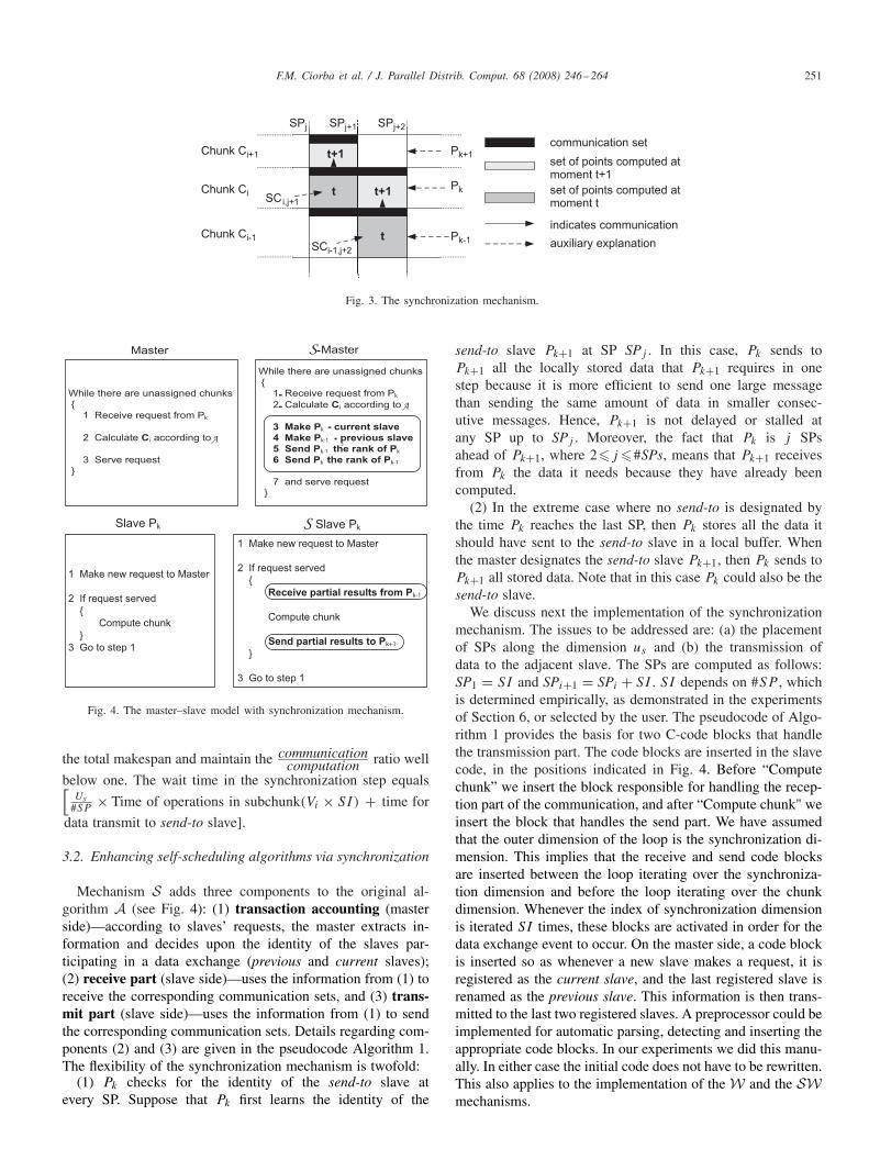
In Fig. 3 chunks i − 1, i, i + 1 are assigned to slavesP, Pk, Pk+1, respectively. The shaded areas denote sets ofiterations that are computed concurrently on different slaves.When Pk reaches the SP SPj+1, after computing SCi,j+1, itsends to Pk+1 the data that Pk+1 needs to begin the executionof SCi+1,j+1, called communication set. Pk sends to Pk+1data only for those iterations of SCi,j+1 on which the iter-ations of SCi+1,j+1 depend on. Communication is incurredonly by those dependence vectors that cross chunks. Note thatno dependence vector can span more than two chunks.

Slave Pk receives from Pk−1 the data Pk requires in orderto proceed with the execution of SCi,j+2. Note that slavesdo not reach the same SP at the same time. For instance, Pk

reaches SPj+1 earlier than Pk+1 and later than Pk−1. Theexistence of SPs leads to a wavefront execution, as shown inFigs. 3 and 5. The choice of SI plays a crucial role in theparallel performance. It should be chosen so as to minimize


t

t t+1

t+1communication set

set of points computed at moment t

set of points computed at moment t+1

indicates communication

auxiliary explanation

SCi,j+1

SCi-1,j+2

Pk+1

Pk

Pk-1

SPj SPj+1 SPj+2

Chunk Ci+1

Chunk Ci-1

Chunk Ci

Fig. 3. The synchronization mechanism.

Fig. 4. The master–slave model with synchronization mechanism.

the total makespan and maintain the communicationcomputation ratio well

below one. The wait time in the synchronization step equals[Us

#SP× Time of operations in subchunk(Vi × SI) + time for

data transmit to send-to slave].

3.2. Enhancing self-scheduling algorithms via synchronization

Mechanism S adds three components to the original al-gorithm A (see Fig. 4): (1) transaction accounting (masterside)—according to slaves’ requests, the master extracts in-formation and decides upon the identity of the slaves par-ticipating in a data exchange (previous and current slaves);(2) receive part (slave side)—uses the information from (1) toreceive the corresponding communication sets, and (3) trans-mit part (slave side)—uses the information from (1) to sendthe corresponding communication sets. Details regarding com-ponents (2) and (3) are given in the pseudocode Algorithm 1.The flexibility of the synchronization mechanism is twofold:

(1) Pk checks for the identity of the send-to slave atevery SP. Suppose that Pk first learns the identity of the

send-to slave Pk+1 at SP SPj . In this case, Pk sends toPk+1 all the locally stored data that Pk+1 requires in onestep because it is more efficient to send one large messagethan sending the same amount of data in smaller consec-utive messages. Hence, Pk+1 is not delayed or stalled atany SP up to SPj . Moreover, the fact that Pk is j SPsahead of Pk+1, where 2�j �#SPs, means that Pk+1 receivesfrom Pk the data it needs because they have already beencomputed.

(2) In the extreme case where no send-to is designated bythe time Pk reaches the last SP, then Pk stores all the data itshould have sent to the send-to slave in a local buffer. Whenthe master designates the send-to slave Pk+1, then Pk sends toPk+1 all stored data. Note that in this case Pk could also be thesend-to slave.

We discuss next the implementation of the synchronizationmechanism. The issues to be addressed are: (a) the placementof SPs along the dimension us and (b) the transmission ofdata to the adjacent slave. The SPs are computed as follows:SP1 = SI and SPi+1 = SPi + SI . SI depends on #SP , whichis determined empirically, as demonstrated in the experimentsof Section 6, or selected by the user. The pseudocode of Algo-rithm 1 provides the basis for two C-code blocks that handlethe transmission part. The code blocks are inserted in the slavecode, in the positions indicated in Fig. 4. Before “Computechunk” we insert the block responsible for handling the recep-tion part of the communication, and after “Compute chunk" weinsert the block that handles the send part. We have assumedthat the outer dimension of the loop is the synchronization di-mension. This implies that the receive and send code blocksare inserted between the loop iterating over the synchroniza-tion dimension and before the loop iterating over the chunkdimension. Whenever the index of synchronization dimensionis iterated SI times, these blocks are activated in order for thedata exchange event to occur. On the master side, a code blockis inserted so as whenever a new slave makes a request, it isregistered as the current slave, and the last registered slave isrenamed as the previous slave. This information is then trans-mitted to the last two registered slaves. A preprocessor could beimplemented for automatic parsing, detecting and inserting theappropriate code blocks. In our experiments we did this manu-ally. In either case the initial code does not have to be rewritten.This also applies to the implementation of the W and the SWmechanisms.


uS

u

SP1

P1

P2

P3

P4

P1

P2

SP2 SP3 SP4 SP5 SP6 SP7 SP8 SP9 SP10 SP11 SP12

P3

P4

1

2

2 3

3

3

4

4

4

4

5

5

5

5

6

6

6

6

7

7

7

8

9

9

9

10

10

11

11

11

11

12

12

12

24

24

24

24

23

23

23

22

22

21

21

21

20

20

20

20

19

19

19

19

18

18

18

18

17

17

17

17

16

16

16

16

14

14 15

15

15

25

25

25 26

26

27

14 15

13

13

22

21

23

22

8

7

8

10

8

9 10

13

12 13

14

Fig. 5. Parallel execution in wavefront fashion.

3.3. Empirical determination of the appropriate #SPs

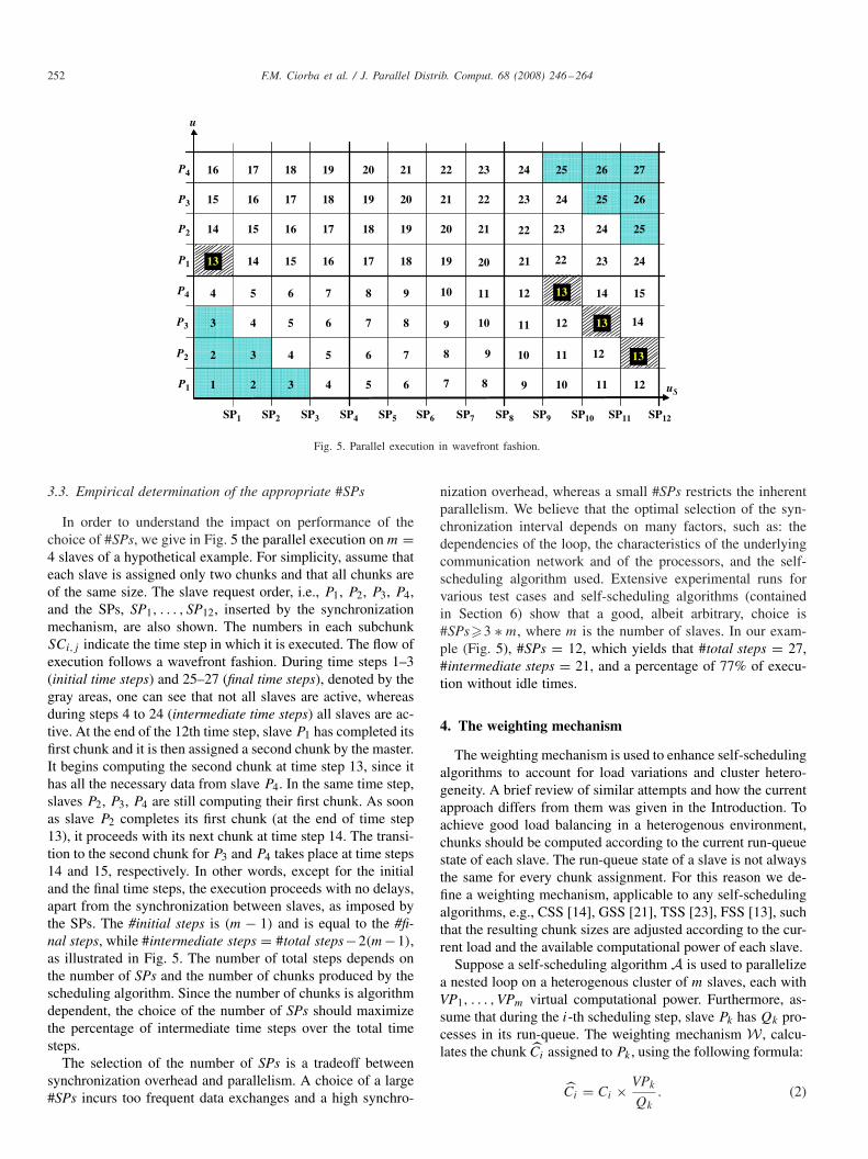
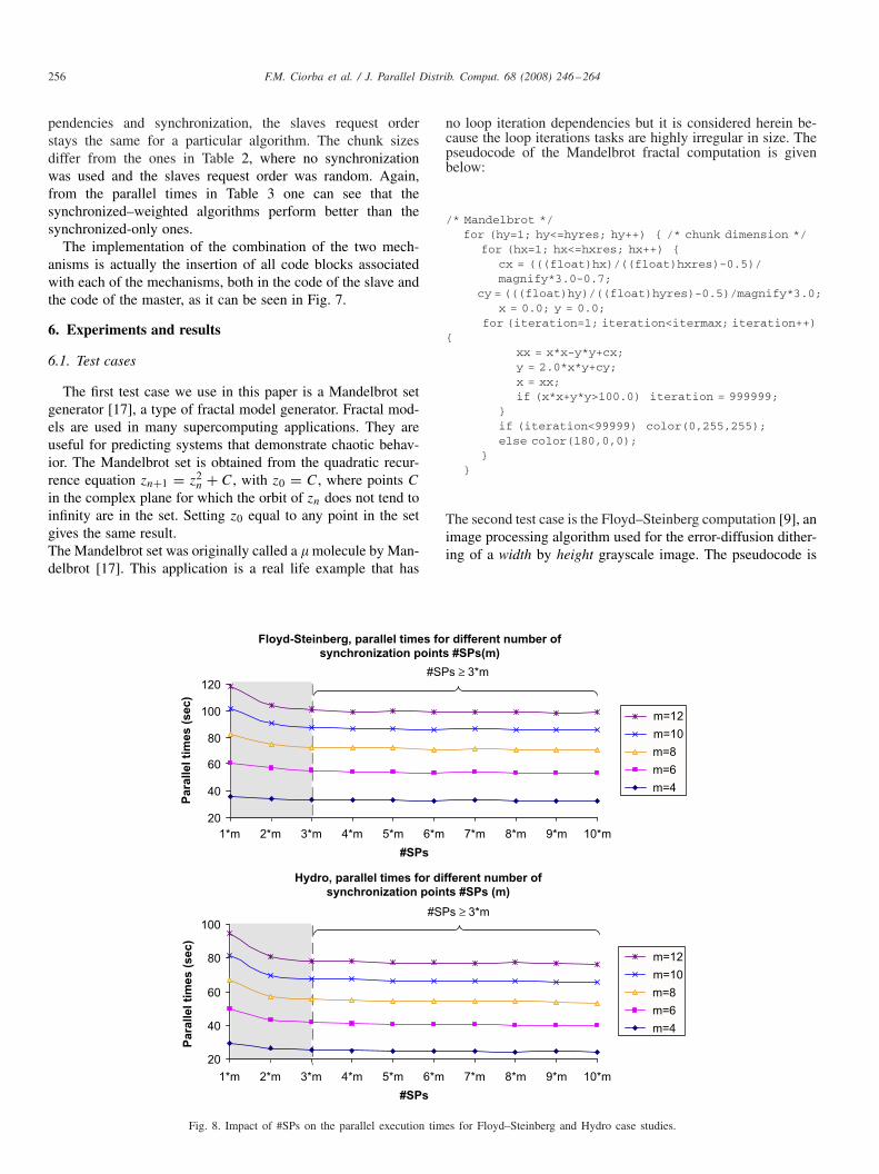
In order to understand the impact on performance of thechoice of #SPs, we give in Fig. 5 the parallel execution on m =4 slaves of a hypothetical example. For simplicity, assume thateach slave is assigned only two chunks and that all chunks areof the same size. The slave request order, i.e., P1, P2, P3, P4,and the SPs, SP1, . . . , SP12, inserted by the synchronizationmechanism, are also shown. The numbers in each subchunkSCi,j indicate the time step in which it is executed. The flow ofexecution follows a wavefront fashion. During time steps 1–3(initial time steps) and 25–27 (final time steps), denoted by thegray areas, one can see that not all slaves are active, whereasduring steps 4 to 24 (intermediate time steps) all slaves are ac-tive. At the end of the 12th time step, slave P1 has completed itsfirst chunk and it is then assigned a second chunk by the master.It begins computing the second chunk at time step 13, since ithas all the necessary data from slave P4. In the same time step,slaves P2, P3, P4 are still computing their first chunk. As soonas slave P2 completes its first chunk (at the end of time step13), it proceeds with its next chunk at time step 14. The transi-tion to the second chunk for P3 and P4 takes place at time steps14 and 15, respectively. In other words, except for the initialand the final time steps, the execution proceeds with no delays,apart from the synchronization between slaves, as imposed bythe SPs. The #initial steps is (m − 1) and is equal to the #fi-nal steps, while #intermediate steps = #total steps−2(m−1),as illustrated in Fig. 5. The number of total steps depends onthe number of SPs and the number of chunks produced by thescheduling algorithm. Since the number of chunks is algorithmdependent, the choice of the number of SPs should maximizethe percentage of intermediate time steps over the total timesteps.

The selection of the number of SPs is a tradeoff betweensynchronization overhead and parallelism. A choice of a large#SPs incurs too frequent data exchanges and a high synchro-

nization overhead, whereas a small #SPs restricts the inherentparallelism. We believe that the optimal selection of the syn-chronization interval depends on many factors, such as: thedependencies of the loop, the characteristics of the underlyingcommunication network and of the processors, and the self-scheduling algorithm used. Extensive experimental runs forvarious test cases and self-scheduling algorithms (containedin Section 6) show that a good, albeit arbitrary, choice is#SPs�3 ∗ m, where m is the number of slaves. In our exam-ple (Fig. 5), #SPs = 12, which yields that #total steps = 27,#intermediate steps = 21, and a percentage of 77% of execu-tion without idle times.

4. The weighting mechanism

The weighting mechanism is used to enhance self-schedulingalgorithms to account for load variations and cluster hetero-geneity. A brief review of similar attempts and how the currentapproach differs from them was given in the Introduction. Toachieve good load balancing in a heterogenous environment,chunks should be computed according to the current run-queuestate of each slave. The run-queue state of a slave is not alwaysthe same for every chunk assignment. For this reason we de-fine a weighting mechanism, applicable to any self-schedulingalgorithms, e.g., CSS [14], GSS [21], TSS [23], FSS [13], suchthat the resulting chunk sizes are adjusted according to the cur-rent load and the available computational power of each slave.

Suppose a self-scheduling algorithm A is used to parallelizea nested loop on a heterogenous cluster of m slaves, each withVP1, . . . ,VPm virtual computational power. Furthermore, as-sume that during the i-th scheduling step, slave Pk has Qk pro-cesses in its run-queue. The weighting mechanism W , calcu-lates the chunk Ci assigned to Pk , using the following formula:

Ci = Ci × VPk

Qk

. (2)


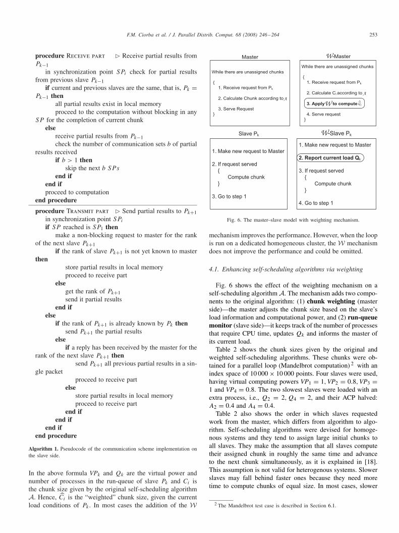
procedure Receive part � Receive partial results fromPk−1

in synchronization point SPi check for partial resultsfrom previous slave Pk−1

if current and previous slaves are the same, that is, Pk =Pk−1 then

all partial results exist in local memoryproceed to the computation without blocking in any

SP for the completion of current chunkelse

receive partial results from Pk−1check the number of communication sets b of partial

results receivedif b > 1 then

skip the next b SP s

end ifend ifproceed to computation

end procedure

procedure Transmit part � Send partial results to Pk+1in synchronization point SPi

if SP reached is SP1 thenmake a non-blocking request to master for the rank

of the next slave Pk+1if the rank of slave Pk+1 is not yet known to master

thenstore partial results in local memoryproceed to receive part

elseget the rank of Pk+1send it partial results

end ifelse

if the rank of Pk+1 is already known by Pk thensend Pk+1 the partial results

elseif a reply has been received by the master for the

rank of the next slave Pk+1 thensend Pk+1 all previous partial results in a sin-

gle packetproceed to receive part

elsestore partial results in local memoryproceed to receive part

end ifend if

end ifend procedure

Algorithm 1. Pseudocode of the communication scheme implementation onthe slave side.

In the above formula VPk and Qk are the virtual power andnumber of processes in the run-queue of slave Pk and Ci isthe chunk size given by the original self-scheduling algorithmA. Hence, Ci is the “weighted” chunk size, given the currentload conditions of Pk . In most cases the addition of the W

c∧

Fig. 6. The master–slave model with weighting mechanism.

mechanism improves the performance. However, when the loopis run on a dedicated homogeneous cluster, the W mechanismdoes not improve the performance and could be omitted.

4.1. Enhancing self-scheduling algorithms via weighting

Fig. 6 shows the effect of the weighting mechanism on aself-scheduling algorithm A. The mechanism adds two compo-nents to the original algorithm: (1) chunk weighting (masterside)—the master adjusts the chunk size based on the slave’sload information and computational power, and (2) run-queuemonitor (slave side)—it keeps track of the number of processesthat require CPU time, updates Qk and informs the master ofits current load.

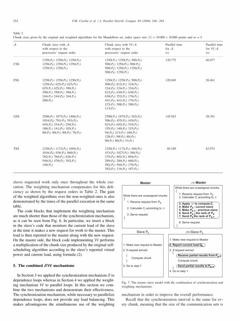
Table 2 shows the chunk sizes given by the original andweighted self-scheduling algorithms. These chunks were ob-tained for a parallel loop (Mandelbrot computation) 2 with anindex space of 10 000 × 10 000 points. Four slaves were used,having virtual computing powers VP1 = 1,VP2 = 0.8,VP3 =1 and VP4 = 0.8. The two slowest slaves were loaded with anextra process, i.e., Q2 = 2, Q4 = 2, and their ACP halved:A2 = 0.4 and A4 = 0.4.

Table 2 also shows the order in which slaves requestedwork from the master, which differs from algorithm to algo-rithm. Self-scheduling algorithms were devised for homoge-nous systems and they tend to assign large initial chunks toall slaves. They make the assumption that all slaves computetheir assigned chunk in roughly the same time and advanceto the next chunk simultaneously, as it is explained in [18].This assumption is not valid for heterogenous systems. Slowerslaves may fall behind faster ones because they need moretime to compute chunks of equal size. In most cases, slower

2 The Mandelbrot test case is described in Section 6.1.


Table 2Chunk sizes given by the original and weighted algorithms for the Mandelbrot set, index space size |J | = 10 000 × 10 000 points and m = 4

A Chunk sizes with A Chunk sizes with W-A Parallel time Parallel timewith respect to the with respect to the for A for W-Aprocessors’ request order processors’ request order (s) (s)

1250(P1) 1250(P2) 1250(P3) 1250(P1) 1250(P3) 500(P4) 120.775 66.077CSS 1250(P4) 1250(P3) 1250(P1) 500(P2) 1250(P3) 500(P2)

1250(P3) 1250(P1) 500(P4) 1250(P1) 1250(P3)500(P4) 1250(P1)

FSS 1250(P1) 1250(P3) 1250(P2) 1250(P1) 1250(P3) 500(P2) 120.849 56.4611250(P4) 625(P3) 625(P3) 500(P4) 812(P3) 324(P2)625(P1) 625(P3) 390(P1) 324(P4) 324(P1) 324(P3)390(P1) 390(P3) 390(P1) 812(P3) 630(P1) 630(P1)244(P3) 244(P4) 244(P1) 630(P4) 252(P3) 176(P1)208(P3) 441(P4) 441(P2) 176(P3)

123(P1) 308(P2) 308(P4)113(P1)

GSS 2500(P1) 1875(P2) 1406(P3) 2500(P1) 1875(P3) 562(P2) 145.943 58.3911054(P4) 791(P3) 593(P3) 506(P4) 455(P4) 410(P2)445(P3) 334(P1) 250(P3) 923(P3) 692(P3) 519(P1)188(P1) 141(P3) 105(P1) 155(P4) 140(P2) 315(P3)80(P3) 80(P1) 80(P3) 78(P1) 94(P4) 213(P1) 160(P3)

120(P1) 90(P3) 80(P2)80(P1) 80(P3) 31(P1)

TSS 1250(P1) 1172(P3) 1094(P2) 1250(P1) 1172(P3) 446(P2) 89.189 63.9741016(P4) 938(P3) 860(P1) 433(P4) 1027(P3) 388(P4)782(P3) 704(P1) 626(P3) 375(P2) 882(P1) 804(P3)548(P4) 470(P2) 392(P1) 299(P4) 286(P2) 660(P1)148(P3) 582(P3) 504(P1) 179(P4)

392(P3) 134(P2) 187(P1)

slaves requested work only once throughout the whole exe-cution. The weighting mechanism compensates for this defi-ciency as shown by the request orders in Table 2. The gainof the weighted algorithms over the non-weighted ones is alsodemonstrated by the times of the parallel execution in the sametable.

The code blocks that implement the weighting mechanismare much shorter than those of the synchronization mechanism,as it can be seen from Fig. 6. In particular, we insert a blockin the slave’s code that monitors the current load of the slaveat the time it makes a new request for work to the master. Thisload is then reported to the master along with the new request.On the master side, the block code implementing W performsa multiplication of the chunk size produced by the original self-scheduling algorithm according to the slave’s reported virtualpower and current load, using formula (2).

5. The combined SW mechanisms

In Section 3 we applied the synchronization mechanism S todependence loops whereas in Section 4 we applied the weight-ing mechanism W to parallel loops. In this section we com-bine the two mechanisms and demonstrate their effectiveness.The synchronization mechanism, while necessary to parallelizedependence loops, does not provide any load balancing. Thismakes advantageous the simultaneous use of the weighting

While there are unassigned chunks {

1. Receive request from Pk

2. Calculate Ci according to A

3. Serve request}

SW-Master

While there are unassigned chunks {

1. Receive request from Pk 2. Calculate Ci according to A

3. Apply W to compute i 4. Make Pk - current slave

5. Make Pk-1 - previous slave 6. Send Pk-1 the rank of Pk 7. Send Pk the rank of Pk-1

8. Serve request}

1. Make new request to Master

2. If request served

{Compute chunk

}

3. Go to step 1

SW-Slave Pk

1. Make new request to Master

2. Report current load Qk

3. If request served {

Receive partial results from Pk-1

Compute chunk

Send partial results to Pk+1}

4. Go to step 1

Master

Slave Pk

C∧

Fig. 7. The master–slave model with the combination of synchronization andweighting mechanisms.

mechanism in order to improve the overall performance.Recall that the synchronization interval is the same for ev-

ery chunk, meaning that the size of the communication sets is


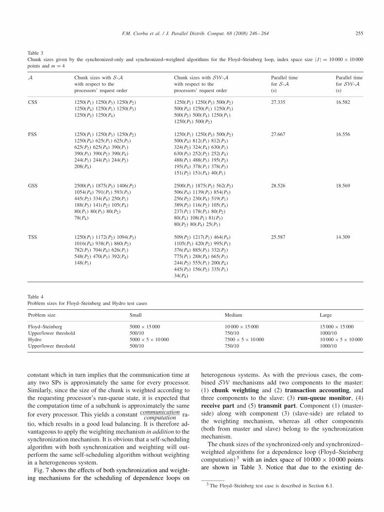
Table 3Chunk sizes given by the synchronized-only and synchronized–weighted algorithms for the Floyd–Steinberg loop, index space size |J | = 10 000 × 10 000points and m = 4

A Chunk sizes with S-A Chunk sizes with SW-A Parallel time Parallel timewith respect to the with respect to the for S-A for SW-Aprocessors’ request order processors’ request order (s) (s)

CSS 1250(P1) 1250(P3) 1250(P2) 1250(P1) 1250(P3) 500(P2) 27.335 16.5821250(P4) 1250(P1) 1250(P3) 500(P4) 1250(P1) 1250(P3)1250(P2) 1250(P4) 500(P2) 500(P4) 1250(P1)

1250(P3) 500(P2)

FSS 1250(P1) 1250(P3) 1250(P2) 1250(P1) 1250(P3) 500(P2) 27.667 16.5561250(P4) 625(P1) 625(P3) 500(P4) 812(P1) 812(P3)625(P2) 625(P4) 390(P1) 324(P2) 324(P4) 630(P1)390(P3) 390(P2) 390(P4) 630(P3) 252(P2) 252(P4)244(P1) 244(P3) 244(P2) 488(P1) 488(P3) 195(P2)208(P4) 195(P4) 378(P1) 378(P3)

151(P2) 151(P4) 40(P1)

GSS 2500(P1) 1875(P3) 1406(P2) 2500(P1) 1875(P3) 562(P2) 28.526 18.5691054(P4) 791(P1) 593(P3) 506(P4) 1139(P1) 854(P3)445(P2) 334(P4) 250(P1) 256(P2) 230(P4) 519(P1)188(P3) 141(P2) 105(P4) 389(P3) 116(P2) 105(P4)80(P1) 80(P3) 80(P2) 237(P1) 178(P3) 80(P2)78(P4) 80(P4) 108(P1) 81(P3)

80(P2) 80(P4) 25(P1)

TSS 1250(P1) 1172(P2) 1094(P3) 509(P2) 1217(P1) 464(P4) 25.587 14.3091016(P4) 938(P1) 860(P2) 1105(P3) 420(P2) 995(P1)782(P3) 704(P4) 626(P1) 376(P4) 885(P3) 332(P2)548(P2) 470(P3) 392(P4) 775(P1) 288(P4) 665(P3)148(P1) 244(P2) 555(P1) 200(P4)

445(P3) 156(P2) 335(P1)34(P4)

Table 4Problem sizes for Floyd–Steinberg and Hydro test cases

Problem size Small Medium Large

Floyd–Steinberg 5000 × 15 000 10 000 × 15 000 15 000 × 15 000Upper/lower threshold 500/10 750/10 1000/10Hydro 5000 × 5 × 10 000 7500 × 5 × 10 000 10 000 × 5 × 10 000Upper/lower threshold 500/10 750/10 1000/10

constant which in turn implies that the communication time atany two SPs is approximately the same for every processor.Similarly, since the size of the chunk is weighted according tothe requesting processor’s run-queue state, it is expected thatthe computation time of a subchunk is approximately the samefor every processor. This yields a constant communication

computation ra-

tio, which results in a good load balancing. It is therefore ad-vantageous to apply the weighting mechanism in addition to thesynchronization mechanism. It is obvious that a self-schedulingalgorithm with both synchronization and weighting will out-perform the same self-scheduling algorithm without weightingin a heterogeneous system.

Fig. 7 shows the effects of both synchronization and weight-ing mechanisms for the scheduling of dependence loops on

heterogenous systems. As with the previous cases, the com-bined SW mechanisms add two components to the master:(1) chunk weighting and (2) transaction accounting, andthree components to the slave: (3) run-queue monitor, (4)receive part and (5) transmit part. Component (1) (master-side) along with component (3) (slave-side) are related tothe weighting mechanism, whereas all other components(both from master and slave) belong to the synchronizationmechanism.

The chunk sizes of the synchronized-only and synchronized–weighted algorithms for a dependence loop (Floyd–Steinbergcomputation) 3 with an index space of 10 000 × 10 000 pointsare shown in Table 3. Notice that due to the existing de-

3 The Floyd–Steinberg test case is described in Section 6.1.


pendencies and synchronization, the slaves request orderstays the same for a particular algorithm. The chunk sizesdiffer from the ones in Table 2, where no synchronizationwas used and the slaves request order was random. Again,from the parallel times in Table 3 one can see that thesynchronized–weighted algorithms perform better than thesynchronized-only ones.

The implementation of the combination of the two mech-anisms is actually the insertion of all code blocks associatedwith each of the mechanisms, both in the code of the slave andthe code of the master, as it can be seen in Fig. 7.

6. Experiments and results

6.1. Test cases

The first test case we use in this paper is a Mandelbrot setgenerator [17], a type of fractal model generator. Fractal mod-els are used in many supercomputing applications. They areuseful for predicting systems that demonstrate chaotic behav-ior. The Mandelbrot set is obtained from the quadratic recur-rence equation zn+1 = z2

n + C, with z0 = C, where points C

in the complex plane for which the orbit of zn does not tend toinfinity are in the set. Setting z0 equal to any point in the setgives the same result.The Mandelbrot set was originally called a � molecule by Man-delbrot [17]. This application is a real life example that has

Floyd-Steinberg, parallel times for different number of

synchronization points #SPs(m)

1*m 2*m 3*m 4*m 5*m 6*m 7*m 8*m 9*m 10*m

#SPs

m=12

m=10

m=8

m=6

m=4

20

120

40

60

80

100

Pa

rallel ti

mes (

sec)

Hydro, parallel times for different number of

synchronization points #SPs (m)

20

100

1*m 2*m 3*m 4*m 5*m 6*m 7*m 8*m 9*m 10*m

#SPs

Para

llel ti

mes (

sec)

m=12

m=10

m=8

m=6

m=4

#SPs ≥ 3*m

#SPs ≥ 3*m

40

60

80

Fig. 8. Impact of #SPs on the parallel execution times for Floyd–Steinberg and Hydro case studies.

no loop iteration dependencies but it is considered herein be-cause the loop iterations tasks are highly irregular in size. Thepseudocode of the Mandelbrot fractal computation is givenbelow:

/* Mandelbrot */for (hy=1; hy<=hyres; hy++) { /* chunk dimension */

for (hx=1; hx<=hxres; hx++) {cx = (((float)hx)/((float)hxres)-0.5)/magnify*3.0-0.7;

cy = (((float)hy)/((float)hyres)-0.5)/magnify*3.0;x = 0.0; y = 0.0;

for (iteration=1; iteration<itermax; iteration++){

xx = x*x-y*y+cx;y = 2.0*x*y+cy;x = xx;if (x*x+y*y>100.0) iteration = 999999;

}if (iteration<99999) color(0,255,255);else color(180,0,0);

}}

The second test case is the Floyd–Steinberg computation [9], animage processing algorithm used for the error-diffusion dither-ing of a width by height grayscale image. The pseudocode is


0

5

10

15

20

25

30

5.4 10.8

Para

llel ti

mes (

sec)

Serial time S-CSS S-FSS S-GSS S-TSS SW-TSS

0

10

20

30

40

50

60

Para

llel ti

mes (

sec)

0

15

30

45

60

75

90

Para

llel ti

mes (

sec)

0

15

30

45

60

75

90

Seri

ala

nd

para

llel

tim

es (

sec

)

0

10

20

30

40

Para

llel ti

mes (

sec)

0

10

20

30

40

50

60

70

Seri

al an

d p

ara

llel

tim

es

(s

ec

)0

10

20

30

40

50

Para

llel ti

mes (

sec)

0

1020

3040

5060

70

Para

llel

tim

es (

sec)

Virtual power

3.6 7.2 9 5.4 10.8

Virtual power

3.6 7.2 9

5.4 10.8

Virtual power

3.6 7.2 95.4 10.8

Virtual power

3.6 7.2 9

5.4 10.8

Virtual power

3.6 7.2 9 5.4 10.8

Virtual power

3.6 7.2 9

Problem size

small medium large

Problem size

small medium large

Floyd-Steinberg, S-CSS, S-FSS, S-GSS,S-TSS

and SW-TSS,5000x15000

Hydro S-CSS, S-FSS, S-GSS, S-TSS and]

SW-TSS, 5000x5x10000

Floyd-Steinberg, S-CSS, S-FSS, S-GSS, S-TSS

and SW-TSS,10000x15000Hydro S-CSS, S-FSS, S-GSS, S-TSS

and SW-TSS, 7500x5x10000

Floyd-Steinberg, S-CSS, S-FSS, S-GSS, S-TSS

and SW-TSS, 15000x15000Hydro S-CSS, S-FSS, S-GSS, S-TSS and

SW-TSS, 10000 x 5 x 10000

Floyd-Steinberg, serial and parallel times for

the three problem sizes,VP=10.8

Hydro, serial and parallel times for the

three problem sizes,VP = 10.8

Serial time S-CSS S-FSS S-GSS S-TSS SW-TSS

Serial time S-CSS S-FSS S-GSS S-TSS SW-TSS Serial time S-CSS S-FSS S-GSS S-TSS SW-TSS



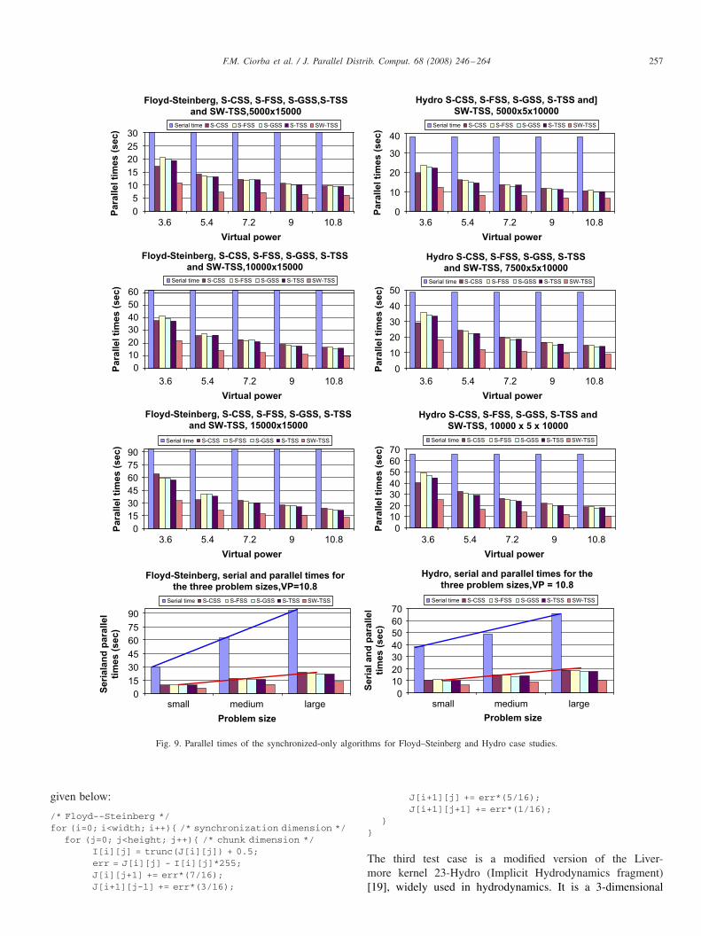
Fig. 9. Parallel times of the synchronized-only algorithms for Floyd–Steinberg and Hydro case studies.

given below:

/* Floyd--Steinberg */for (i=0; i<width; i++){ /* synchronization dimension */

for (j=0; j<height; j++){ /* chunk dimension */I[i][j] = trunc(J[i][j]) + 0.5;err = J[i][j] - I[i][j]*255;J[i][j+1] += err*(7/16);J[i+1][j-1] += err*(3/16);

J[i+1][j] += err*(5/16);J[i+1][j+1] += err*(1/16);

}}

The third test case is a modified version of the Liver-more kernel 23-Hydro (Implicit Hydrodynamics fragment)[19], widely used in hydrodynamics. It is a 3-dimensional


Table 5Speedups for Floyd–Steinberg and Hydro test cases

Test case VP S-CSS S-FSS S-GSS S-TSS SW-TSS

Floyd–Steinberg 3.6 1.45 1.57 1.59 1.63 2.865.4 2.76 2.35 2.33 2.47 4.357.2 2.81 2.92 3.09 3.10 5.399 3.41 3.50 3.49 3.70 6.27

10.8 3.95 4.07 4.27 4.34 7.09

Hydro 3.6 1.64 1.33 1.42 1.47 2.615.4 2.02 2.10 2.16 2.28 4.047.2 2.53 2.57 2.72 2.75 4.739 3.01 3.07 3.33 3.29 5.43

10.8 3.49 3.49 3.72 3.69 6.16

Mandelbrot, TSS vs W-TSS

0

50

100

150

200

Para

llel ti

mes (

sec)

TSS W-TSS

10000x10000 12500x12500 15000x15000

0

50

100

150

200

5.4 7.2 10.83.6 5.4 7.2 9 10.83.6 5.4 7.2 9 10.8

Para

llel ti

mes (

sec)

CSS W-CSS

10000x10000 12500x12500 15000x15000

Mandelbrot, FSS vs W-FSS

0

50

100

150P

ara

llel ti

mes (

sec)

FSS W-FSS

10000x10000 12500x12500 15000x15000

Mandelbrot, GSS vs W-GSS

0

100

200

300

Para

llel ti

mes (

sec)

GSS W-GSS

10000x10000 12500x12500 15000x15000

Mandelbrot, W-CSS,W-FSS,W-GSS,W-TSS

0

30

60

90

120

150

180

Para

llel ti

mes (

sec)

W-CSS W-GSS W-FSS W-TSS

10000x10000 12500x12500 15000x15000

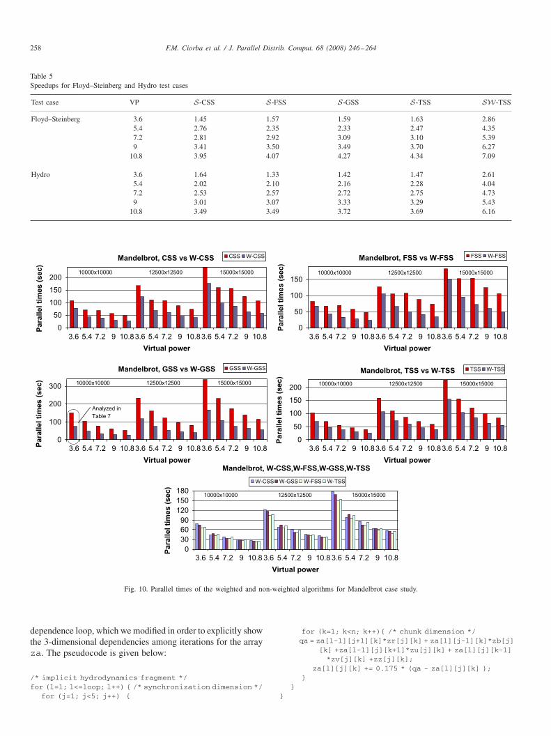
Analyzed in

Table 7

Virtual power

3.6 9 5.4 7.2 10.83.6 5.4 7.2 9 10.83.6 5.4 7.2 9 10.8

Virtual power

3.6 9

5.4 7.2 10.83.6 5.4 7.2 9 10.83.6 5.4 7.2 9 10.8

Virtual power

3.6 95.4 7.2 10.83.6 5.4 7.2 9 10.83.6 5.4 7.2 9 10.8

Virtual power

3.6 9

5.4 7.2 10.8 3.6 5.4 7.2 9 10.8 3.6 5.4 7.2 9 10.8

Virtual power

3.6 9

Mandelbrot, CSS vs W-CSS

Fig. 10. Parallel times of the weighted and non-weighted algorithms for Mandelbrot case study.

dependence loop, which we modified in order to explicitly showthe 3-dimensional dependencies among iterations for the arrayza. The pseudocode is given below:

/* implicit hydrodynamics fragment */for (l=1; l<=loop; l++) { /* synchronization dimension */

for (j=1; j<5; j++) {

for (k=1; k<n; k++){ /* chunk dimension */qa = za[l-1][j+1][k]*zr[j][k] + za[l][j-1][k]*zb[j]

[k] +za[l-1][j][k+1]*zu[j][k] + za[l][j][k-1]*zv[j][k] +zz[j][k];

za[l][j][k] += 0.175 * (qa - za[l][j][k] );}

}}


Table 6Gain of the weighted over the non-weighted algorithms for the Mandelbrot test case

Test Problem VP S-CSS S-GSS S-FSS S-TSScase size vs SW-CSS (%) vs SW-GSS (%) vs SW-FSS (%) vs SW-TSS (%)

Mandelbrot 10 000 × 10 000 3.6 27 50 18 335.4 38 54 37 347.2 43 57 52 329 48 53 52 35

10.8 43 52 52 34

12 500 × 12 500 3.6 27 50 18 335.4 38 54 37 347.2 44 57 53 309 47 54 52 35

10.8 44 52 53 34

15 000 × 15 000 3.6 27 50 18 335.4 38 54 37 347.2 45 57 53 319 49 54 52 35

10.8 46 52 54 33

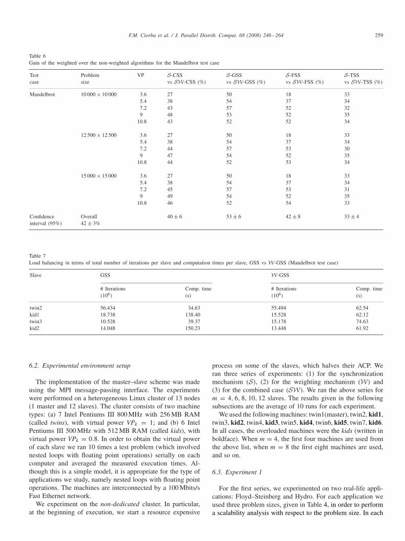
Confidence Overall 40 ± 6 53 ± 6 42 ± 8 33 ± 4interval (95%) 42 ± 3%

Table 7Load balancing in terms of total number of iterations per slave and computation times per slave, GSS vs W-GSS (Mandelbrot test case)

Slave GSS W-GSS

# Iterations Comp. time # Iterations Comp. time(106) (s) (106) (s)

twin2 56.434 34.63 55.494 62.54kid1 18.738 138.40 15.528 62.12twin3 10.528 39.37 15.178 74.63kid2 14.048 150.23 13.448 61.92

6.2. Experimental environment setup

The implementation of the master–slave scheme was madeusing the MPI message-passing interface. The experimentswere performed on a heterogeneous Linux cluster of 13 nodes(1 master and 12 slaves). The cluster consists of two machinetypes: (a) 7 Intel Pentiums III 800 MHz with 256 MB RAM(called twins), with virtual power VPk = 1; and (b) 6 IntelPentiums III 500 MHz with 512 MB RAM (called kids), withvirtual power VPk = 0.8. In order to obtain the virtual powerof each slave we ran 10 times a test problem (which involvednested loops with floating point operations) serially on eachcomputer and averaged the measured execution times. Al-though this is a simple model, it is appropriate for the type ofapplications we study, namely nested loops with floating pointoperations. The machines are interconnected by a 100 Mbits/sFast Ethernet network.

We experiment on the non-dedicated cluster. In particular,at the beginning of execution, we start a resource expensive

process on some of the slaves, which halves their ACP. Weran three series of experiments: (1) for the synchronizationmechanism (S), (2) for the weighting mechanism (W) and(3) for the combined case (SW). We ran the above series form = 4, 6, 8, 10, 12 slaves. The results given in the followingsubsections are the average of 10 runs for each experiment.

We used the following machines: twin1(master), twin2, kid1,twin3, kid2, twin4, kid3, twin5, kid4, twin6, kid5, twin7, kid6.In all cases, the overloaded machines were the kids (written inboldface). When m = 4, the first four machines are used fromthe above list, when m = 8 the first eight machines are used,and so on.

6.3. Experiment 1

For the first series, we experimented on two real-life appli-cations: Floyd–Steinberg and Hydro. For each application weused three problem sizes, given in Table 4, in order to performa scalability analysis with respect to the problem size. In each


Floyd-Steinberg,S-CSS vs SW-CSS

0

20

40

60

3.6 5.4 7.2 10.83.6 5.4 7.2 9 10.83.6 5.4 7.2 9 10.8

Para

llel ti

mes (

sec)

S-CSS SW-CSS

15000x5000 15000x10000 15000x15000

Floyd-Steinberg,S-GSS vs SW-GSS

0

20

40

60

Para

llel ti

mes (

sec)

S-GSS SW-GSS

15000x5000 15000x10000 15000x15000

Floyd-Steinberg, S-FSS vs SW-FSS

0

20

40

60

Para

llel ti

mes (

sec)

S-FSS SW-FSS

15000x5000 15000x10000 15000x15000

Floyd-Steinberg, S-TSS vs SW-TSS

0

20

40

60

Para

llel ti

mes (

sec)

S-TSS SW-TSS

15000x5000 15000x10000 15000x15000

Floyd-Steinberg, SW-CSS, SW-FSS, SW-GSS and SW-TSS

05

1015

2025

3035

Para

llel ti

mes (

sec)

SW -C SW-FSS SW-GSS SW-TSS

15000x5000 15000x10000 15000x15000

Analyzed in Table 9

Virtual power

9 3.6 5.4 7.2 10.83.6 5.4 7.2 9 10.83.6 5.4 7.2 9 10.8

Virtual power

9

3.6 5.4 7.2 10.83.6 5.4 7.2 9 10.83.6 5.4 7.2 9 10.8

Virtual power

93.6 5.4 7.2 10.83.6 5.4 7.2 9 10.83.6 5.4 7.2 9 10.8

Virtual power

9

3.6 5.4 7.2 10.8 3.6 5.4 7.2 9 10.8 3.6 5.4 7.2 9 10.8

Virtual power

9

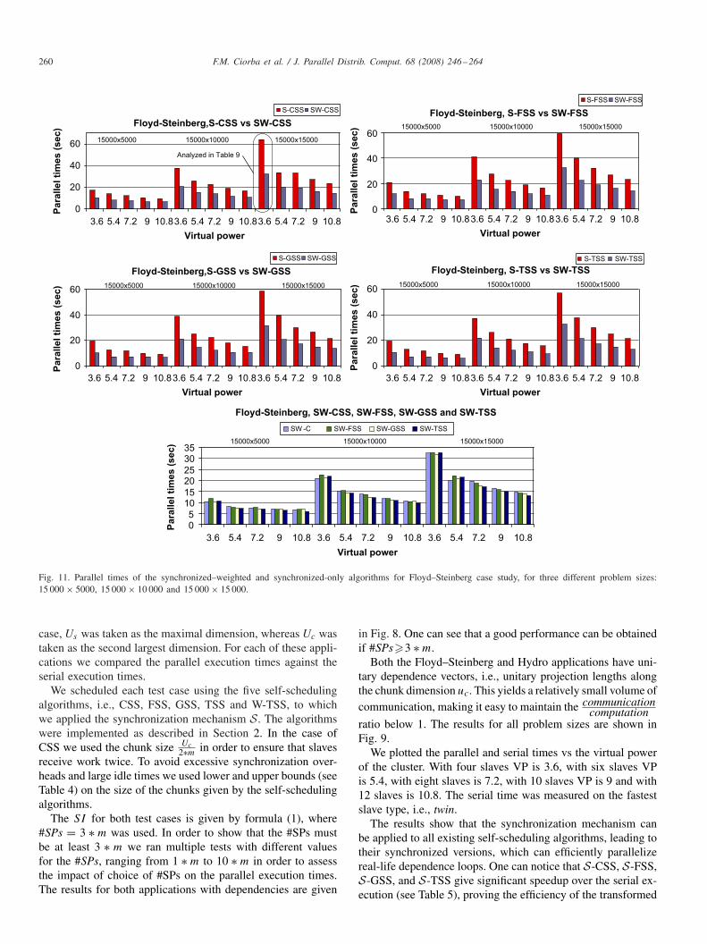
Fig. 11. Parallel times of the synchronized–weighted and synchronized-only algorithms for Floyd–Steinberg case study, for three different problem sizes:15 000 × 5000, 15 000 × 10 000 and 15 000 × 15 000.

case, Us was taken as the maximal dimension, whereas Uc wastaken as the second largest dimension. For each of these appli-cations we compared the parallel execution times against theserial execution times.

We scheduled each test case using the five self-schedulingalgorithms, i.e., CSS, FSS, GSS, TSS and W-TSS, to whichwe applied the synchronization mechanism S. The algorithmswere implemented as described in Section 2. In the case ofCSS we used the chunk size Uc

2∗min order to ensure that slaves

receive work twice. To avoid excessive synchronization over-heads and large idle times we used lower and upper bounds (seeTable 4) on the size of the chunks given by the self-schedulingalgorithms.

The SI for both test cases is given by formula (1), where#SPs = 3 ∗ m was used. In order to show that the #SPs mustbe at least 3 ∗ m we ran multiple tests with different valuesfor the #SPs, ranging from 1 ∗ m to 10 ∗ m in order to assessthe impact of choice of #SPs on the parallel execution times.The results for both applications with dependencies are given

in Fig. 8. One can see that a good performance can be obtainedif #SPs�3 ∗ m.

Both the Floyd–Steinberg and Hydro applications have uni-tary dependence vectors, i.e., unitary projection lengths alongthe chunk dimension uc. This yields a relatively small volume ofcommunication, making it easy to maintain the communication

computationratio below 1. The results for all problem sizes are shown inFig. 9.

We plotted the parallel and serial times vs the virtual powerof the cluster. With four slaves VP is 3.6, with six slaves VPis 5.4, with eight slaves is 7.2, with 10 slaves VP is 9 and with12 slaves is 10.8. The serial time was measured on the fastestslave type, i.e., twin.

The results show that the synchronization mechanism canbe applied to all existing self-scheduling algorithms, leading totheir synchronized versions, which can efficiently parallelizereal-life dependence loops. One can notice that S-CSS, S-FSS,S-GSS, and S-TSS give significant speedup over the serial ex-ecution (see Table 5), proving the efficiency of the transformed


0

20

40

3.6 5.4 7.2 10.83.6 5.4 7.2 9 10.83.6 5.4 7.2 9 10.8

Para

llel ti

mes (

sec)

S-CSS SW-CSS

10000x5x5000 10000x5x7500 10000x5x10000

0

20

40

Para

llel

tim

es (

sec)

S-GSS SW-GSS

10000x5x5000 10000x5x7500 10000x5x10000

0

20

40

Para

llel ti

mes (

sec)

S-FSS SW-FSS

10000x5x5000 10000x5x7500 10000x5x10000

0

20

40

Para

llel

tim

es (

sec)

S-TSS SW-TSS

10000x5x5000 10000x5x7500 10000x5x10000

0

5

10

15

20

25

30

Para

llel ti

mes (

sec)

SW-CSS SW-FSS SW-GSS SW-TSS

10000x5x5000 10000x5x7500 10000x5x10000

Analyzedin Table 9

9

Virtual power

3.6 5.4 7.2 10.83.6 5.4 7.2 9 10.83.6 5.4 7.2 9 10.89

Virtual power

3.6 5.4 7.2 10.83.6 5.4 7.2 9 10.83.6 5.4 7.2 9 10.89

Virtual power

3.6 5.4 7.2 10.83.6 5.4 7.2 9 10.83.6 5.4 7.2 9 10.89

Virtual power

3.6 5.4 7.2 10.8 3.6 5.4 7.2 9 10.8 3.6 5.4 7.2 9 10.89

Virtual power

Hydro,S-CSS vsSW-CSS Hydro,S-FSS vs SW-FSS

Hydro,S-GSS vs SW-GSS Hydro,S-TSS vs SW-TSS

Hydro, SW-CSS, SW-FSS, SW-GSS and SW-TSS

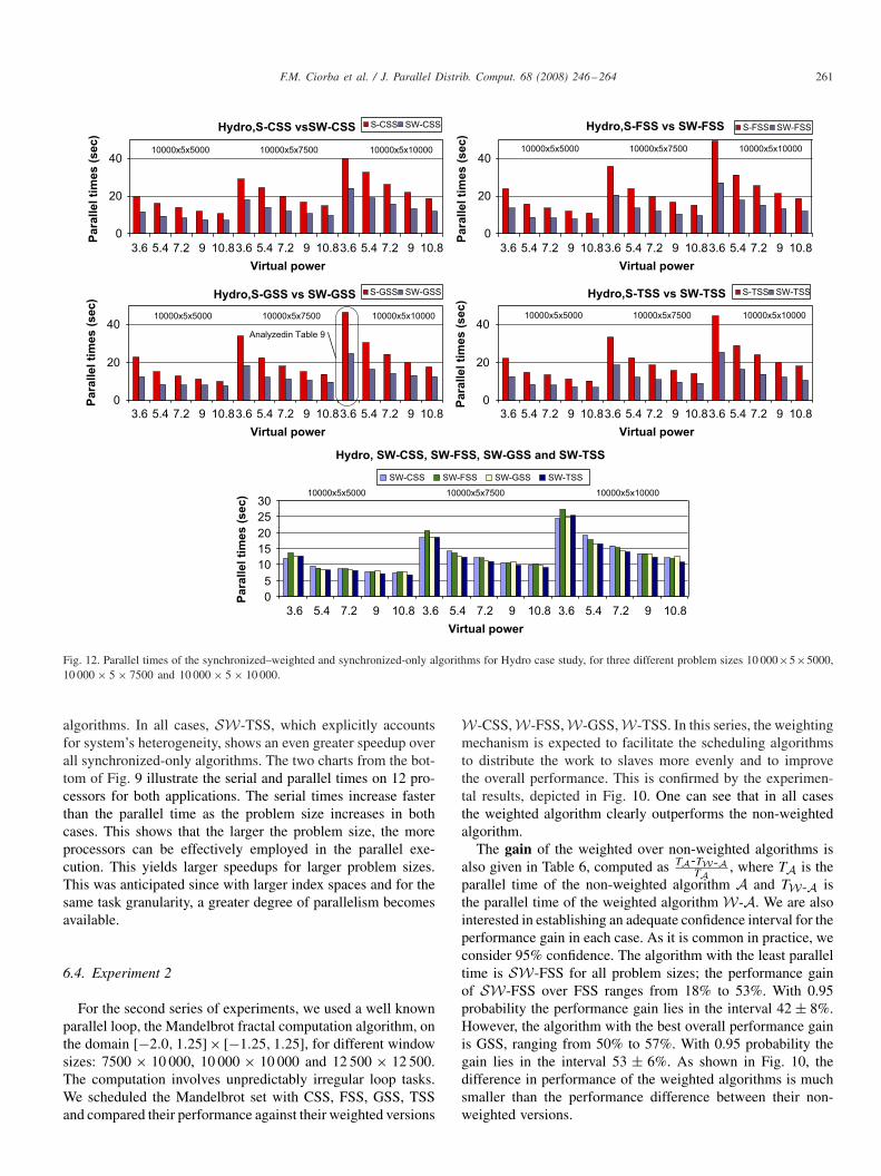
Fig. 12. Parallel times of the synchronized–weighted and synchronized-only algorithms for Hydro case study, for three different problem sizes 10 000×5×5000,10 000 × 5 × 7500 and 10 000 × 5 × 10 000.

algorithms. In all cases, SW-TSS, which explicitly accountsfor system’s heterogeneity, shows an even greater speedup overall synchronized-only algorithms. The two charts from the bot-tom of Fig. 9 illustrate the serial and parallel times on 12 pro-cessors for both applications. The serial times increase fasterthan the parallel time as the problem size increases in bothcases. This shows that the larger the problem size, the moreprocessors can be effectively employed in the parallel exe-cution. This yields larger speedups for larger problem sizes.This was anticipated since with larger index spaces and for thesame task granularity, a greater degree of parallelism becomesavailable.

6.4. Experiment 2

For the second series of experiments, we used a well knownparallel loop, the Mandelbrot fractal computation algorithm, onthe domain [−2.0, 1.25]× [−1.25, 1.25], for different windowsizes: 7500 × 10 000, 10 000 × 10 000 and 12 500 × 12 500.The computation involves unpredictably irregular loop tasks.We scheduled the Mandelbrot set with CSS, FSS, GSS, TSSand compared their performance against their weighted versions

W-CSS, W-FSS, W-GSS, W-TSS. In this series, the weightingmechanism is expected to facilitate the scheduling algorithmsto distribute the work to slaves more evenly and to improvethe overall performance. This is confirmed by the experimen-tal results, depicted in Fig. 10. One can see that in all casesthe weighted algorithm clearly outperforms the non-weightedalgorithm.

The gain of the weighted over non-weighted algorithms isalso given in Table 6, computed as TA-TW-A

TA , where TA is theparallel time of the non-weighted algorithm A and TW-A isthe parallel time of the weighted algorithm W-A. We are alsointerested in establishing an adequate confidence interval for theperformance gain in each case. As it is common in practice, weconsider 95% confidence. The algorithm with the least paralleltime is SW-FSS for all problem sizes; the performance gainof SW-FSS over FSS ranges from 18% to 53%. With 0.95probability the performance gain lies in the interval 42 ± 8%.However, the algorithm with the best overall performance gainis GSS, ranging from 50% to 57%. With 0.95 probability thegain lies in the interval 53 ± 6%. As shown in Fig. 10, thedifference in performance of the weighted algorithms is muchsmaller than the performance difference between their non-weighted versions.


Table 8Gain of the synchronized–weighted over the synchronized-only algorithms for the Floyd–Steinberg and Hydro test cases

Test Problem VP S-CSS S-GSS S-FSS S-TSScase size vs SW-CSS (%) vs SW-GSS (%) vs SW-FSS (%) vs SW-TSS (%)

Floyd–Steinberg 15 000 × 5000 3.6 39 47 43 455.4 42 43 44 44

7.2 37 40 35 409 34 27 34 36

10.8 31 23 28 35

15 000 × 7500 3.6 44 46 45 425.4 41 42 44 457.2 39 45 38 429 37 40 37 38

10.8 36 30 36 38

15 000 × 10 000 3.6 50 46 45 435.4 41 48 44 437.2 41 42 41 429 39 43 40 41

10.8 38 36 38 39

Confidence Overall 39 ± 2 40 ± 3 40 ± 2 41 ± 2interval (95%) 40 ± 1

Hydro 10 000 × 5 × 5000 3.6 40 46 43 445.4 43 44 44 447.2 39 37 37 419 37 29 36 38

10.8 32 23 29 34

10 000 × 5 × 7500 3.6 38 46 43 445.4 43 45 44 467.2 40 37 39 429 37 29 38 38

10.8 35 30 35 36

10 000 × 5 × 10 000 3.6 40 47 45 445.4 42 47 44 437.2 40 41 41 429 39 33 38 39

10.8 37 30 37 40

Confidence Overall 39 ± 2 38 ± 4 40 ± 2 41 ± 2interval (95%) 39 ± 1

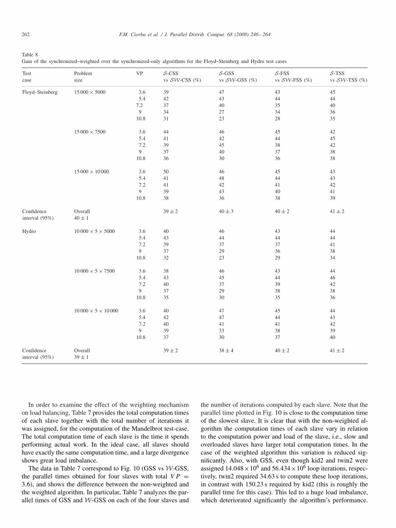
In order to examine the effect of the weighting mechanismon load balancing, Table 7 provides the total computation timesof each slave together with the total number of iterations itwas assigned, for the computation of the Mandelbrot test-case.The total computation time of each slave is the time it spendsperforming actual work. In the ideal case, all slaves shouldhave exactly the same computation time, and a large divergenceshows great load imbalance.

The data in Table 7 correspond to Fig. 10 (GSS vs W-GSS,the parallel times obtained for four slaves with total V P =3.6), and shows the difference between the non-weighted andthe weighted algorithm. In particular, Table 7 analyzes the par-allel times of GSS and W-GSS on each of the four slaves and

the number of iterations computed by each slave. Note that theparallel time plotted in Fig. 10 is close to the computation timeof the slowest slave. It is clear that with the non-weighted al-gorithm the computation times of each slave vary in relationto the computation power and load of the slave, i.e., slow andoverloaded slaves have larger total computation times. In thecase of the weighted algorithm this variation is reduced sig-nificantly. Also, with GSS, even though kid2 and twin2 wereassigned 14.048×106 and 56.434×106 loop iterations, respec-tively, twin2 required 34.63 s to compute these loop iterations,in contrast with 150.23 s required by kid2 (this is roughly theparallel time for this case). This led to a huge load imbalance,which deteriorated significantly the algorithm’s performance.


Table 9Load balancing in terms of total number of iterations per slave and computation times per slave, S-FSS vs SW-FSS

Test Slave # Iterations (106) Comp. time (s) # Iterations (106) Comp. time (s)

S-CSS S-CSS SW-CSS SW-CSS

Floyd–Steinberg twin2 59.93 19.25 89.90 28.88kid1 59.93 62.22 29.92 30.86twin3 59.93 19.24 74.92 24.06kid2 44.95 46.30 29.92 29.08

S-GSS S-GSS SW-GSS SW-GSS

Hydro twin2 84.50 15.32 117.94 21.39kid1 78.38 42.60 38.03 22.49twin3 62.69 17.44 106.48 20.75kid2 73.58 33.72 36.41 19.46

Unlike GSS, W-GSS execution times for all slaves are aboutthe same which confirms that W-GSS indeed achieves goodload balancing.

6.5. Experiment 3

For the third series of experiments we repeat the first series,applying now the W mechanism to all synchronized-only al-gorithms. In particular, we schedule the Floyd–Steinberg andHydro test cases with the following synchronized–weightedalgorithms: SW-CSS, SW-FSS, SW-GSS and SW-TSS.The results in Figs. 11 and 12 show that in all cases thesynchronized–weighted algorithms clearly outperform theirsynchronized-only counterparts. One can notice that all SWalgorithms give comparable parallel times.

The above results are also illustrated in Table 8, which showsthe gain of SW-A over S-A, computed as TS-A−TSW-A

TS-A , whereTS-A is the parallel time of the synchronized-only algorithm Aand TSW-A is the parallel time of the synchronized–weightedalgorithm SW-A. Confidence intervals are also given in thesame Table, both with respect to every algorithm and overallconfidence intervals per test case.

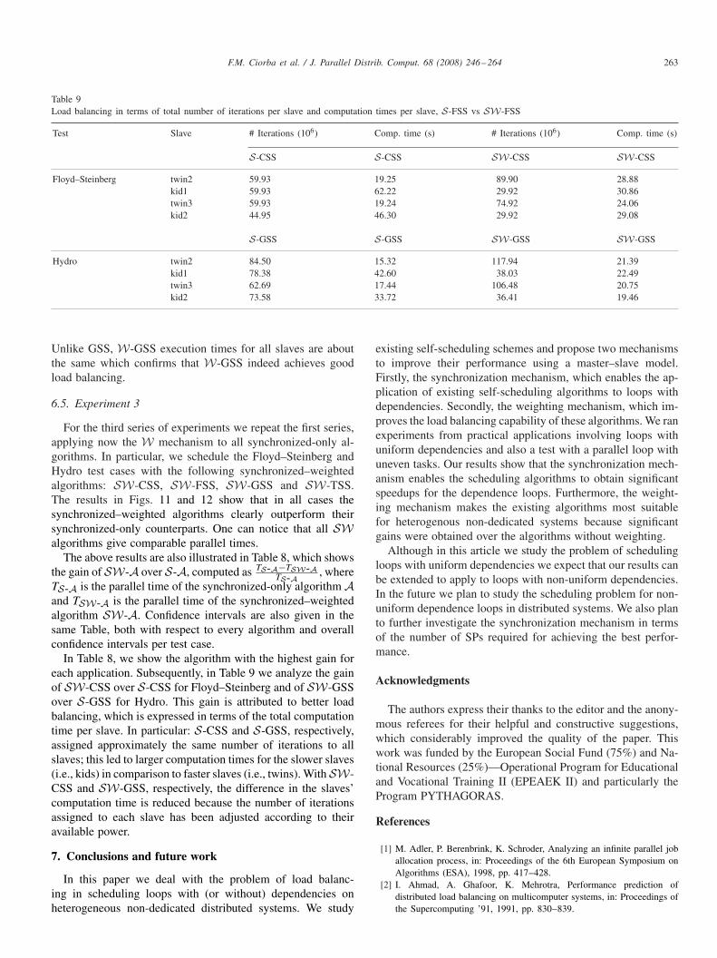
In Table 8, we show the algorithm with the highest gain foreach application. Subsequently, in Table 9 we analyze the gainof SW-CSS over S-CSS for Floyd–Steinberg and of SW-GSSover S-GSS for Hydro. This gain is attributed to better loadbalancing, which is expressed in terms of the total computationtime per slave. In particular: S-CSS and S-GSS, respectively,assigned approximately the same number of iterations to allslaves; this led to larger computation times for the slower slaves(i.e., kids) in comparison to faster slaves (i.e., twins). With SW-CSS and SW-GSS, respectively, the difference in the slaves’computation time is reduced because the number of iterationsassigned to each slave has been adjusted according to theiravailable power.

7. Conclusions and future work

In this paper we deal with the problem of load balanc-ing in scheduling loops with (or without) dependencies onheterogeneous non-dedicated distributed systems. We study

existing self-scheduling schemes and propose two mechanismsto improve their performance using a master–slave model.Firstly, the synchronization mechanism, which enables the ap-plication of existing self-scheduling algorithms to loops withdependencies. Secondly, the weighting mechanism, which im-proves the load balancing capability of these algorithms. We ranexperiments from practical applications involving loops withuniform dependencies and also a test with a parallel loop withuneven tasks. Our results show that the synchronization mech-anism enables the scheduling algorithms to obtain significantspeedups for the dependence loops. Furthermore, the weight-ing mechanism makes the existing algorithms most suitablefor heterogenous non-dedicated systems because significantgains were obtained over the algorithms without weighting.

Although in this article we study the problem of schedulingloops with uniform dependencies we expect that our results canbe extended to apply to loops with non-uniform dependencies.In the future we plan to study the scheduling problem for non-uniform dependence loops in distributed systems. We also planto further investigate the synchronization mechanism in termsof the number of SPs required for achieving the best perfor-mance.

Acknowledgments

The authors express their thanks to the editor and the anony-mous referees for their helpful and constructive suggestions,which considerably improved the quality of the paper. Thiswork was funded by the European Social Fund (75%) and Na-tional Resources (25%)—Operational Program for Educationaland Vocational Training II (EPEAEK II) and particularly theProgram PYTHAGORAS.

References

[1] M. Adler, P. Berenbrink, K. Schroder, Analyzing an infinite parallel joballocation process, in: Proceedings of the 6th European Symposium onAlgorithms (ESA), 1998, pp. 417–428.

[2] I. Ahmad, A. Ghafoor, K. Mehrotra, Performance prediction ofdistributed load balancing on multicomputer systems, in: Proceedings ofthe Supercomputing ’91, 1991, pp. 830–839.


[3] I. Banicescu, Z. Liu, Adaptive factoring: a dynamic scheduling methodtuned to the rate of weight changes, in: Proceedings of the HighPerformance Computing Symposium 2000, Washington, USA, 2000, pp.122–129.

[4] I. Banicescu, V. Velusamy, J. Devaprasad, On the scalability of dynamicscheduling scientific applications with adaptive weighted factoring,Cluster Comput. J. Networks Software Tools Appl. 6 (3) (2003)215–226.

[5] A.T. Chronopoulos, R. Andonie, M. Benche, D. Grosu, A classof distributed self-scheduling schemes for heterogeneous clusters, in:Proceedings of the 3rd IEEE International Conference on ClusterComputing (CLUSTER 2001), Newport Beach, CA, USA, 2001.

[6] A.T. Chronopoulos, S. Penmatsa, J. Xu, S. Ali, Distributed loopscheduling schemes for heterogeneous computer systems, ConcurrencyComput. Pract. Experience 18 (7) (2006) 771–785.

[7] F.M. Ciorba, T. Andronikos, I. Riakiotakis, A.T. Chronopoulos,G. Papakonstantinou, Dynamic multiphase scheduling for heterogeneousclusters, in: Proceedings of the 20th IEEE International Parallel &Distributed Processing Symposium (IPDPS 2006), Rhodes, Greece, 2006.

[8] D.L. Eager, E.D. Lazowska, Adaptive load sharing in homogeneousdistributed systems, IEEE Trans. Software Eng. 12 (5) (1986).

[9] R.W. Floyd, L. Steinberg, An adaptive algorithm for spatial grey scale,Proc. Soc. Inf. Display 17 (1976) 75–77.

[10] M. Harchol-Balter, A.B. Downey, Exploiting process lifetimedistributions for dynamic load balancing, ACM Trans. Comput. Systems15 (3) (1997) 253–285.

[11] C.-J. Hou, K.G. Shin, Load sharing with consideration of future taskarrivals in heterogeneous distributed real-time systems, IEEE Trans.Comput. 49 (9) (1994) 1076–1090.

[12] S.F. Hummel, J. Schmidt, R.N. Uma, J. Wein, Load-sharing inheterogeneous systems via weighted factoring, in: Proceedings of the8th Annual ACM Symposium on Parallel Algorithms and Architectures,1996.

[13] S.F. Hummel, E. Schonberg, L.E. Flynn, Factoring: a method forscheduling parallel loops, Commun. ACM 35 (8) (1992) 90–101.

[14] C.P. Kruskal, A. Weiss, Allocating independent subtasks on parallelprocessors, IEEE Trans. Software Eng. 11 (10) (1985) 1001–1016.

[15] Y.K. Kwok, I. Ahmad, Static scheduling algorithms for allocatingdirected task graphs to multiprocessors, ACM Comput. Surveys 31 (4)(1999) 406–471.

[16] Q. Lu, S.-M. Lau, K.-S. Leung, Dynamic load distribution using antitasksand load state vectors, Concurrency: Pract. Experience 10 (14) (1998)1251–1269.

[17] B.B. Mandelbrot, Fractal Geometry of Nature, W. H. Freeman & Co,New York, August 1988.

[18] E.P. Markatos, T.J. LeBlanc, Using processor affinity in loop schedulingon shared-memory multiprocessors, IEEE Trans. Parallel Distrib. Systems5 (4) (1994) 379–400.

[19] F.H. McMahon, The Livermore Fortran Kernels: A Computer Testof the Numerical Performance Range, Lawrence Livermore NationalLaboratory, Livermore, CA, UCRL-53745, 1986.

[20] D. Petkov, R. Harr, S. Amarasinghe, Efficient pipelining of nested loops:unroll-and-squash, in: Proceedings of the 16th IEEE International Parallel& Distributed Processing Symposium (IPDPS 2002), Ft. Lauderdale, FL,USA, 2002.

[21] C.D. Polychronopoulos, D.J. Kuck, Guided self-scheduling: a practicalself-scheduling scheme for parallel supercomputers, IEEE Trans.Comput. C-36 (12) (1987) 1425–1439.

[22] E. Silva, M. Gerla, Queueing network models for load balancing indistributed systems, J. Parallel Distrib. Comput. 12 (1991) 24–38.

[23] T.H. Tzen, L.M. Ni, Trapezoid self-scheduling: a practical schedulingscheme for parallel compilers, IEEE Trans. Parallel Distrib. Systems 4(1) (1993) 87–98.

[24] J.-L. Wang, L.-T. Lee, Y.-J. Huang, Load balancing policies inheterogeneous distributed systems, in: Proceedings of the 26thSoutheastern Symposium System Theory, 1994.

Florina M. Ciorba received her Diploma inComputer Engineering from the University ofOradea, Romania, in 2001. Since 2002 she isa Ph.D. candidate at the National TechnicalUniversity of Athens, Greece. Her researchinterests include parallel and distributed highperformance computing, resource management,scheduling and load balancing. She is an IEEEstudent member since 2004.

Ioannis Riakiotakis received his B.Sc. in Elec-tronics Engineering in 1999 and his M.Sc. inCommunication Engineering and Signal Pro-cessing in 2000 both from the University ofPlymouth (UK). Since 2002 he is a Ph.D. can-didate at the National Technical University ofAthens (Greece). His research interests includedistributed computing, dynamic load balancingalgorithms.

Theodore Andronikos received his Degree inElectrical and Computer Engineering and hisPh.D. from the Computer Science Division,School of Electrical and Computer Engineer-ing, National Technical University of Athens.He is currently a lecturer at the Department ofInformatics of the Ionian University. His re-search interests include parallel and distributedcomputing, internet programming, algorithmiccomplexity and formal verification of reactivesystems.

George Papakonstantinou received hisDiploma in Electrical Engineering from the Na-tional Technical University of Athens in 1964,the PII Diploma in Electronic Engineering fromPhilips International Institute in 1966, and hisM.Sc. in Electronic Engineering from NUFFIC,the Netherlands in 1967. In 1971, he receivedhis Ph.D. in Computer Engineering from theNational Technical University of Athens. Hehas worked as a Research Scientist at theGreek Atomic Energy Commission/ComputerDivision (1969–1984), as Director of the Com-puter Division at the Greek Atomic Energy

Commission (1981–1984). From 1984 he serves as a Professor of ComputerEngineering at the National Technical University of Athens. His current re-search interests include knowledge engineering, syntactic pattern recognition,logic design, embedded systems, as well as parallel architectures and lan-guages. He has published more than 270 papers in international referred jour-nals and in proceedings of international conferences. Dr. Papakonstantinouhas over 200 citations.

Anthony T. Chronopoulos received his Ph.D. atthe University of Illinois in Urbana-Champaignin 1987. He is a senior member of the IEEE andthe ACM. He has published 40 journals and 45refereed conference proceedings publications inthe areas of distributed systems, game theory,networks and security, parallel processing. Hehas been awarded 15 federal/state governmentresearch grants. His work is cited in more than260 nonco-authors’ research articles.

Enhancing self-scheduling algorithms via synchronization and weighting (PLEASE REFERENCE IN YOUR...

Documents

Transcript of Enhancing self-scheduling algorithms via synchronization and weighting (PLEASE REFERENCE IN YOUR...