Nonlinear Dynamics and Synchronization of Bidirectionally ...
207
UNIVERSITAT DE LES ILLES BALEARS DEPARTAMENT DE FISICA Nonlinear Dynamics and Synchronization of Bidirectionally Coupled Semiconductor Lasers Tesi presentada per Ra´ ul Vicente, en el De- partament de F´ ısica de la Universitat de les Illes Balears, per optar al grau de Doctor en F´ ısica. Palma, June 2006
-
Upload
khangminh22 -
Category
Documents
-
view
4 -
download
0
Transcript of Nonlinear Dynamics and Synchronization of Bidirectionally ...

UNIVERSITAT DE LES ILLES BALEARSDEPARTAMENT DE FISICA
Nonlinear Dynamics and Synchronizationof Bidirectionally Coupled Semiconductor
Lasers
Tesi presentada per Raul Vicente, en el De-partament de Fısica de la Universitat de lesIlles Balears, per optar al grau de Doctor enFısica.
Palma, June 2006


El director de tesi Claudio R. Mirasso Santos Titular Universitaride la Universitat de les Illes Balears certifica que aquesta tesi doc-toral ha estat realitzada pel Sr. Raul Vicente Zafra, i perque quediconstancia escrita firma
a Palma 5 de Juny de 2006.
Claudio R. Mirasso Santos


A mis padres, por recordarme tantas veces quesabe mas el zorro por viejo que por zorro.


Agradecimientos
En primer lugar, y no podıa ser de otra manera, quisiera agradecer a Claudio Mi-rasso la confianza, el respeto y la amistad que me ha brindado durante todos estosanos. Este trabajo se ha beneficiado directamente de su diligente coordinacion ydel clima que ha sabido generar para que el intercambio de ideas y discusionesfueran bienvenidos en cualquier momento. Tambien me quiero acordar aquı delafecto expresado hacia mi por Alejandra y Nico (mi mamita y hermanito en LosAngeles) cuando estaba lejos de casa.
Este trabajo no hubiera sido el mismo sin la gran ayuda y constante revision deJosep Mulet, a quien le agradezco profundamente todas las horas de provechosasdiscusiones que hemos pasado y de quien espero se me haya pegado algo de susaber hacer.
A Toni Perez le debo probablemente el estar escribiendo estas lineas ahoramismo. El fue quien me hablo por primera vez de un proyecto relacionado conlaseres caoticos y demas. Son incontables las horas de trabajo cientıfico y de di-version que hemos compartido dentro de la EFE y fuera de ella. Por toda la ayudaprestada en tantas ocasiones, miles de GRACIAS!
A Pere Colet, con quien he tenido la oportunidad de colaboraren alguna oca-sion, me gustarıa tambien mostrarle mi gratitud por estar siempre abierto a es-cuchar y debatir cualquier tipo de problema cientıfico con el que uno le vaya amolestar a su despacho.
En definitiva, gracias a todo el personal del IMEDEA y del Departament deFısica de la UIB con quienes siempre me he encontrado todas las puertas abier-tas. Tambien quiero agradecer explıcitamente a Maxi (aunque todavıa no tengala camiseta ni la gorra del IMEDEA...) el hecho de que nos obligue a ir a losseminarios. En cinco anos de charlas uno llega a desarrollar un interes por lo in-terdisciplinar difıcilmente fomentable de alguna otra manera.
Quisiera tambien mencionar a Javier Buldu por su ayuda y colaboracion tanto
vii

viii Agradecimientos
en trabajos cientıficos como por lo bien que lo hemos pasado en distintas confe-rencias por el mundo (Atenas, Pavia, Metz, etc...) y a Jordi Garcıa-Ojalvo, MarıaCarme Torrent y Cristina por hacer de la UPC en Terrasa un sitio tan acogedor yagradable para hacer ciencia.
Ingo Fischer ha sido sin duda uno de los artıfices de que este trabajo llegue abuen puerto. Le agradezco enormemente no solo la amabilidad y paciencia que hatenido conmigo sino tambien la calidad y cantidad de las ideas que me ha comu-nicado desde que le conocı y algunas de las cuales se encuentran en las siguientespaginas. Marc Sciamanna es otro gran investigador de quienuno puede apren-der mucho y a quien mucho la colaboracion que tuvimos sobre la dinamica deVCSELs. A Michael Peil tambien le agradezco las discusionesque hemos tenidojuntos y la fiabilidad de sus resultados experimentales que han permitido validar yfomentar muchos de los resultados aquı expuestos.
El Profesor Jia-ming Liu fue quien me dio la oportunidad de visitar UCLA(la segunda mejor universidad del mundo despues de la UIB) y vivir por una tem-porada (casi nueve meses) en Estados Unidos. Es a el y a mis companeros delaboratorio Howard, Steven, Shuo, Frank, Nelson, Margaret, Juan, Rose Mary,Manuel y Rider a quienes les debo gran parte de que mi estanciaen Los Angelessencillamente maravillosa. No tengo palabras para agradecer el trato y carino allırecibido por la genial cantante de Jazz y mejor companera depiso, Shirlee. To-davıa echo de menos a Matilda, las visitas al Cafe Roma y tus cinnamon rolls!
De los companeros en la EFE que voy a decir despues de que me hayan te-nido que aguantar durante casi 5 anos!!! Mis companeros decubıculo, desde lossolares como Inigo, Jaume, Toni o Pep, hasta los mas interdisciplinares como Pau,Iacyel y Dani se merecen lo mejor. Todos los miembros de la EFE, los nuevos ylos veteranos, han sido excelentes a la hora de crear un agradable lugar de traba-jo. Siempre me acordare de las tertulias con Lolo, del incombustible Pierre, o deJuanjo guardando la bandera de la EFE... Gracias tambien alduo Tessone-Adrian(o Linux vs Windows) por aclararme cualquier duda informatica casi en tiemporeal. A Yanne tambien le quiero expresar mi simpatıa ya quehe disfrutado muchohablando con el sobre muchos temas que iban desde los retos del Africa de hoyhasta divagaciones de cosmologıa o mecanica cuantica.
Ya en el plano completamente personal, como me iba a olvidar del G5: Mi-guel, Nieto, Jose, Alfredo y Juanmi con quienes desde que nos conocimos en SanJose he crecido y compartido tanto, incluso ese inolvidable viaje en coche por todaCalifornia y alrededores. Lo que pasa en Las Vegas se queda enLas Vegas! DavidEsteban es otro de esos viejos amigos que siempre estan ahıcuando se los necesita.

ix
Muy especialmente quiero agradecer a Dana Alic su amistad y comprensionmientras escribıa esta tesis. Gracias de verdad.
Lo mejor del curso del CAP (despues de la V de Godwing por supuesto) es elhaber conocido a Penelope Glamour (na Joana), na Marineta, na Lida y en Xavi.Lo que nos hemos reıdo juntos y lo que nos queda. Gracias por todo chicos!
En definitiva, gracias a todos aquellos de los que he aprendido algo y a quienesme tienen que soportar voluntaria o involuntariamente cadadıa. Por cierto, Zidaneprobablemente nunca llegue a leer esto pero gracias por esosmagnıficos domingospor la tarde que los miembros de la EFE imitamos tan mal en los partidillos de losjueves.
A mi familia, padres, hermanos y sobrinos, decirles que sin ellos no serıa naday que esto por pequeno que sea, va por ellos!
Junio 2006, Palma, Raul Vicente Zafra


Acknowledgments
First, I would like to thank Claudio Mirasso for the trust, respect, and friendshipthat he has offered to me during all these years. This work hasbeen directly ben-efitted from his diligent coordination and from the environment that he has gen-erated to foment the exchanges of ideas and discussions at any moment. I wouldalso like to mention the goodwill and affection I received from Alejandra and Nicowhen I was far away from home.
This work would have never been the same without the help and constant su-pervision of Josep Mulet, to whom I profoundly thank all the time we have spenton fruitful discussions and improving this work.
Toni Perez is probably the responsible of the fact that I am writing this wordsright now. He was the first in telling me about a project related to chaotic lasers andmore... The hours we have spent working hard on a scientific problem or havingfun inside or out of the EFE Agency are just countless. For allthe help, THANKYOU!
To Pere Colet, with whom I have had the opportunity to collaborate with, Iwould like to express my acknowledgments for his open mind and willing to listenand discuss about almost any problem with which one can visithim in his office.
In summary, thanks to everybody at IMEDEA and the Departament de Fısicawhere I have always found all the doors opened. I would also like to particularlythank Maxi (even though I am still waiting for the IMEDEA T-shirt and cap) toforce us to attend to all the seminars. In five years of talks one develops an interestfor interdisciplinary research very difficult to promote inany other way.
I would also like to mention Javier Buldu for his help and collaboration in bothscientific works and social life around the world (Athens, Pavia, Metz, etc...) andto Jordi Garcıa-Ojalvo, Marıa Carme Torrent and Cristinato make the UPC at Ter-rassa a homy and comfortable place to do Science.
xi

xii Acknowledgments
Ingo Fischer have been without any doubt one of the persons who contributemost to this work. I really thank his kindness and the huge quality and quantityof the ideas he has transmitted to me since we met and which some of them arecollected in the following pages. Marc Sciamanna is anothergreat researcher fromwhom one can really learn and I thank him a lot the collaboration on the VCSELsdynamics. I thank Michael Peil the profitable discussions wehave maintained andthe quality of his experimental research that has lead to thevalidation and deepermotivation of the results exposed here.
Professor Jia-ming Liu was the person who gave me the unforgettable oppor-tunity to visit UCLA (the second best university after UIB) and to live for a while(almost nine months) in the amazing city of Los Angeles. He and my lab matesHoward, Steven, Shuo, Frank, Nelson, Margaret, Juan, Rose Mary, Manuel andRider (thanks for the tequila amigo) are big responsibles for the great time I hadin LA. I have no words to express my gratitude towards the kindly treat and sup-port I received from the genial Jazz singer and best roommate, Shirlee. I still missMatilda, the visits to Cafe Roma, and your cinnamon rolls!
What can I say about my EFE mates after they stood me for so long. My officemates, from the Solar guys Inigo, Jaume, Toni and Pep, to themore interdisci-plinary souls Pau, Iacyel and Dani deserve a place in heaven.All the people fromthe Agency, the newcomers and the veterans, have been excellent companions andhave created a great working place. I will always remember the countless laughs Ishared with Lolo, the energy of Pierre or Juanjo the tireless... Thanks also to thepair Tessone-Adrian (or Linux vs Windows) for kindly clarifying in real time allthe computer science doubts I had. I would also like to express my sympathy toYanne for the enjoyable discussions about the most diverse topics.
In the personal dimension how could I forget about the G5 team: Miguel, Ni-eto, Jose, Alfredo and Juanmi with whom I have grown up sincewe met in SanJose, including a great trip we made through California andsurroundings. Whathappen in Vegas, stay in Vegas! David Esteban is a good and oldfriend who hashelped me in many cases. Thanks guys!
Very specially I would like to thank Dana Alic her friendshipand support whilewriting this these. My most sincere and profound gratitude for everything Danuca!
The best from the CAP classes (of course, after the Godwing V lesson) it hasbeen to meet Penelope Glamour (na Joana), na Marineta Cafeina, na Lida GPS,and en Xavi (alias en Farril Carril). We have shared great moments and I hope thatthere is still a lot more to come.

xiii
In conclusion, thanks to everybody from who I have learned something in thislife and to those who stand me everyday voluntarily or not. Zidane, you will neverread this words but thanks for these wonderful Sunday afternoons.
To my family, parents, brother, syster, and nephews, I wouldlike to tell youthat I would not be anything without you, and this work even small is dedicated toyou!
June 2006, Palma, Raul Vicente Zafra


Contents
1 Preface 1
I Introduction 9
2 An overview to synchronization 11
2.1 Definition . . . . . . . . . . . . . . . . . . . . . . . . . . . . . . 112.2 Why does synchronization take place? . . . . . . . . . . . . . . . 142.3 The hallmarks of synchronization . . . . . . . . . . . . . . . . . 15
2.3.1 Frequency locking . . . . . . . . . . . . . . . . . . . . . 162.3.2 Phase locking . . . . . . . . . . . . . . . . . . . . . . . . 182.3.3 Instantaneous amplitude and phase of a signal . . . . . . .19
2.4 Different kinds of synchronization . . . . . . . . . . . . . . . . .212.5 Measures and detection of sync . . . . . . . . . . . . . . . . . . . 242.6 Oscillation quenching . . . . . . . . . . . . . . . . . . . . . . . . 26
3 Delayed interactions 29
3.1 Delay Differential Equations . . . . . . . . . . . . . . . . . . . . 303.1.1 Definition . . . . . . . . . . . . . . . . . . . . . . . . . . 303.1.2 Classification and main features . . . . . . . . . . . . . . 30
3.2 Stability theory . . . . . . . . . . . . . . . . . . . . . . . . . . . 323.2.1 Linear stability of retarded functional differential equations 323.2.2 D-Subdivision method . . . . . . . . . . . . . . . . . . . 34
3.3 Oscillation quenching revisited . . . . . . . . . . . . . . . . . . .35
4 Basics of bifurcations 37
4.1 Definition . . . . . . . . . . . . . . . . . . . . . . . . . . . . . . 374.2 Classification . . . . . . . . . . . . . . . . . . . . . . . . . . . . 38
4.2.1 Basic local bifurcations for flows and maps . . . . . . . . 394.2.2 Global bifurcations . . . . . . . . . . . . . . . . . . . . . 45
xv

xvi CONTENTS
4.3 Symmetry methods for bifurcations . . . . . . . . . . . . . . . . 46
5 Basics of lasers 49
5.1 Once upon a laser . . . . . . . . . . . . . . . . . . . . . . . . . . 495.2 Semiconductor lasers . . . . . . . . . . . . . . . . . . . . . . . . 51
5.2.1 Introduction . . . . . . . . . . . . . . . . . . . . . . . . . 515.2.2 Semiconductor laser rate equations . . . . . . . . . . . . 525.2.3 Polarization of light . . . . . . . . . . . . . . . . . . . . 54
II Results 57
6 Mutually-coupled semiconductor lasers: stability, route to chaos, andsynchronization 59
6.1 Model . . . . . . . . . . . . . . . . . . . . . . . . . . . . . . . . 616.1.1 The system . . . . . . . . . . . . . . . . . . . . . . . . . 616.1.2 Modeling equations . . . . . . . . . . . . . . . . . . . . . 626.1.3 Fixed points of the model . . . . . . . . . . . . . . . . . 64
6.2 Bidirectional coupling without feedback . . . . . . . . . . . .. . 656.2.1 Stability analysis of fixed points . . . . . . . . . . . . . . 666.2.2 Stability diagrams . . . . . . . . . . . . . . . . . . . . . 716.2.3 Periodic solutions and the route to chaos . . . . . . . . . . 766.2.4 Mutual entrainment of laser instabilities . . . . . . . . .. 796.2.5 Experimental results . . . . . . . . . . . . . . . . . . . . 826.2.6 Conclusions . . . . . . . . . . . . . . . . . . . . . . . . . 85
6.3 Bidirectional coupling with feedback . . . . . . . . . . . . . . .. 866.3.1 Stability diagrams . . . . . . . . . . . . . . . . . . . . . 866.3.2 Death by delay . . . . . . . . . . . . . . . . . . . . . . . 936.3.3 Synchronization . . . . . . . . . . . . . . . . . . . . . . 976.3.4 Experimental results . . . . . . . . . . . . . . . . . . . . 1066.3.5 Conclusions . . . . . . . . . . . . . . . . . . . . . . . . . 107
7 Mutually-coupled VCSELs: a study of synchronization in vectorialoscillators 109
7.1 Model and parameters . . . . . . . . . . . . . . . . . . . . . . . . 1107.2 Polarization switching and hysteresis . . . . . . . . . . . . . .. . 112
7.2.1 Coupling-induced PS . . . . . . . . . . . . . . . . . . . . 1127.2.2 Detuning-induced polarization dynamics . . . . . . . . . 118
7.3 Dynamics accompanying polarization switchings . . . . . .. . . 1197.3.1 Spin-flip rate influence . . . . . . . . . . . . . . . . . . . 121
7.4 Misalignment effects . . . . . . . . . . . . . . . . . . . . . . . . 125

CONTENTS xvii
7.5 Synchronization . . . . . . . . . . . . . . . . . . . . . . . . . . . 1297.6 Conclusions . . . . . . . . . . . . . . . . . . . . . . . . . . . . . 131
8 Synchronization of three mutually-coupled semiconductor lasers 133
8.1 Model . . . . . . . . . . . . . . . . . . . . . . . . . . . . . . . . 1348.2 Dynamics of three semiconductor lasers in an open-end configura-
tion . . . . . . . . . . . . . . . . . . . . . . . . . . . . . . . . . 1368.2.1 Coupling-induced instabilities . . . . . . . . . . . . . . . 1368.2.2 Robustness of the synchronization solution . . . . . . . .1418.2.3 Synchronization for asymmetric coupling times . . . . .. 1468.2.4 Synchronization of semiconductor lasers with feedback . . 148
8.3 The role of network on the synchronization properties . .. . . . . 1508.3.1 Open-end arrays . . . . . . . . . . . . . . . . . . . . . . 1508.3.2 Ring networks . . . . . . . . . . . . . . . . . . . . . . . 1548.3.3 The symmetry connection . . . . . . . . . . . . . . . . . 154
8.4 Bidirectional chaos-based communications with semiconductorlasers . . . . . . . . . . . . . . . . . . . . . . . . . . . . . . . . 161
8.5 Conclusions . . . . . . . . . . . . . . . . . . . . . . . . . . . . . 166
9 Concluding remarks 167
Bibliography 173
List of Figures 179
Curriculum Vitae i


Chapter 1
Preface
SYNCHRONIZATION is the dynamical process by which two or more oscillatorsadjust their rhythms due to a weak interaction [1]. Part of the universality of
this phenomenom comes from the vast variety of systems able to experience thiseffect. By just thinking about the many different objects present in Nature thatperiodically repeat its state, i.e., oscillate, and that these systems are generally notisolated but interacting with each other, it is easy to recognize that synchroniza-tion must be acting on a huge number of structures at different scales [2]. Froman audience in which people tend to accommodate their claps to sound in unison[3], to thousands of pacemaker cells in our heart tissue spiking their action poten-tials together to induce a beat in our heart every few seconds, the objects able toexperience sync cover a wide spectrum [4]. Today, synchronization is studied inhundreds of examples of engineering and physical sciences,as well as in the lessunderstood and challenging biological and social entities[1,4,5].
To explain the basics of synchronization let us take a brief glance to a modernadaptation of one of the earliest examples in which sync was ever noticed morethan three centuries ago. The historical setup consisted ofa set of two pendulumclocks hanging from a common support [1]. In a more recent andmusical versionof such an experiment we consider two almost identical pendulum metronomesresting on a light wooden board which lies on two soda cans [6]. The setup canbe seen in Figure 1.1. Usually, one can set any of the metronomes to beat fromfew decades to hundreds of times per minute. By prescribing slightly different fre-quencies of oscillation to both metronomes, one expects that their pendula wouldremain swinging at different rhythms. However, when both timekeepers sit on thesame movable platform, it is usually observed that their formerly uncorrelated au-dible ticks start to approach in time, and eventually they end up being heard inunison. Then, we say that the metronomes have synchronized.The almost un-noticeable motion of the base is responsible for the momentum transfer, or “com-munication”, between both metronomes in such a way that it usually favors the
1

2 Preface
simultaneous swing of both pendulum bobs. How long it takes the system to reachthis state and whether this sympathy of swings occurs with the pendula bobs mov-ing toward the same or opposite directions, are questions whose solution dependson the details of the system, such as the mass of the pendula and the friction ofthe base. But the important point here is that this effect is by no means a matter ofchance. It develops for a determined range of disaccord in the frequencies of bothmetronomes before coupling them, and when it appears is stable to small perturba-tions of the system. It is this robust capability of a precisematching of oscillationsbetween different systems what the concept of synchronization is about.
Figure 1.1. A pair of sim-ilar metronomes laying ona light wooden base is avery simple and illustrativesystem demonstrating syn-chronization. The horizon-tal movement of the plat-form is the responsible forcoupling the motion of bothoscillators. After Ref. [5].
Since it was first formally described by Christiaan Huygens in 1665 [1] syn-chronization, understood as an agreement or entrainment ofrhythms, has beenextensively reported in very diverse fields. It is exploitedfor hightech applicationsin devices such as electric power generators or Josephson junctions SQUIDs1 [1].By the same phenomenon, chemical oscillations are able to beentrained to a givenperiod, as in the famous Belousov-Zhabotinsky reaction subject to optical forc-ing [1]. In other order of complexity, physiological levelsof different hormonesand proteins are governed by biological clocks, which are able to adjust and locktheir rhythms to the frequency of an appropriate external modulation. In a clearexample, circadian rhythms in our bodies are consequences of the adaptation ofour biological clocks to the 24-hours day-night oscillation of variables such astemperature or illuminance [1,4,5]. Spectacular cases of synchronization are alsofound in large populations of living organisms. The simultaneous chirp of somesinger crickets in a house yard or the coincident flashing of thousands of fireflies(Figure 1.2) in the riverbanks of southeast Asia have amazedthe scientists and thegeneral public for centuries [5]. Sometimes, however, the appearance of synchro-nization has unexpected side effects that are not funny at all. In its opening day, alateral excitation of the London’s Millennium Bridge was induced by the hundredsof people‘s synchronized walking pace. The amplitude of theoscillation of the
1SQUID stands for Superconducting QUantum Interfering Device and it is the most sensitivemagnetic field detector known to man.

3
bridge exceeded seven centimeters and it was enough to spread an unpleasant andeven scaring feeling among the pedestrians [5].
The examples commented before
Figure 1.2. Thousands of fireflies from theLampyridaefamily flashing simultaneouslyin a cave in New Zealand.
concern very diverse systems and nev-ertheless, all of them share the charac-teristic of falling into the category of ei-ther periodic oscillators or rotators. Ifthis was the full story, even occupyingan important place in science and tech-nology, synchronization would have notbecome one of the hotest research top-ics in nonlinear science as it is consid-ered today. A great boost that was toshake the investigation in synchroniza-tion came in the early nineties, fromprobably one of the more unexpectedways.
In February of 1990, Lou Pecora andTom Carroll, from the US Naval Re-search Laboratory at Washington D.C.,published in Physical Review Letters a paper entitled “Synchronization in ChaoticSystems” [7]. By that time, just to have in mind the idea of synchronizing two ofsuch systems could be easily qualified by any expert in the field as a hopeless task.Chaos is a dynamical regime in which a system becomes extremely sensitive to ini-tial conditions and reveals an unpredictable and random-like behavior, even thoughthe underlying model of a system exhibiting chaos can be deterministic and verysimple2. If there was a system challenging the capability of synchronizing thatwas a chaotic one. And yet, Pecora and Carroll were right. They demonstratedthat chaotic synchronization could be achieved by driving or replacing one of thevariables of a chaotic system with a variable of another similar chaotic device. Apair of Lorenz systems, being considered as one of the most paradigmatic modelsin chaos theory, was selected in their paper to numerically prove chaotic synchro-nization for the first time.
The illustration of the convergence of two chaotic trajectories to the same val-ues opened a new perspective to fundamental questions in thepreviously indepen-dent chaos and synchronization themes. Applications, on the other hand, foundin the newborn chaotic synchronization a promising tool to be exploited in spreadspectrum communications and cryptography. In this last field, the main idea con-sists of hiding or encrypting a message into the noise-like trace of a chaotic outputand use the chaotic synchronization property by an authorized part to recover themessage. The masking of the message to be encoded is usually performed at the
2Only three nonlinear ordinary differential equations or even one non-invertible map are enoughto produce a chaotic flow of data in a computer.

4 Preface
physical layer by the “mix” of the signal with a chaotic carrier generated by a non-linear element. After the transmission over an appropriatecommunication chan-nel, the recovery of the message is based on the synchronization phenomenon, bywhich a receiver, quite similar to the transmitter, is able to reproduce the chaoticpart of the transmitted signal. Then, by a proper comparisonof the input and out-put at the receiver, an efficient decoding of the message can be performed. In 1993,two researchers from the MIT experimentally demonstrated the working principleof this private communication scheme [8]. They used analog electronic circuitsemulating the behavior of two chaotic Lorenz systems. However, electronic cir-cuits suffer from severe drawbacks that make them unsuitable for practical com-munication schemes. Electronic circuits have in general a restricted bandwidthlimited to a few tens of kHz, and moreover their output signalis not suited formodern communication transmission lines based on optical fibers. A natural ques-tion was then, is there any source with a large bandwidth, inherently nonlinear andready to be used in real communications standards?
The answer had five letters, LASER. Since May 1960, when Theodore H.Maiman succeeded for the very first time in History to maintain a laser actionin a ruby crystal3, these devices have truly revolutionized industries such as com-munications or medicine. In 1994, Pere Colet and Rajarshi Roy working then atthe Georgia Institute of Technology, proposed a solid-state laser system to demon-strate synchronization and message encryption in the optical domain [9]. However,very soon the attention moved toward another class of lasersmuch more promisingfor this and other applications in consumer electronics andinformation technology,the Semiconductor Lasers (SLs).
While in the beginning of the laser
Figure 1.3. Typical semiconductor laserwith its package capsule.
era the dream of any laser scientist wasto achieve a stable, high-intensity andspectral pure laser beam, the modernperspective today is to promote the un-derstanding and control of the laser in-stabilities, i.e., deviations from its con-tinuous wave (CW) emission. In this re-spect, it took little time to realize thatSLs are nonlinear dynamical systems ableto generate a rich variety of behaviors
and that we could actually take a great advantage from it. Thegeneration of ultra-short pulses, all-optical processing of information, creation of carrier signals in themicrowave range, or cryptography based on chaotic communications are just a fewexamples of applications that benefitted from our present control on the dynamicsof lasers. The scenarios leading to dynamical instabilities in a SL are diverse.Either by modulating its injection current, injecting light into its active material,
3Interestingly several investigators though to have demonstrated by that time that laser emissioncould not be generated with ruby as an amplifier medium.

5
or feeding back part of the emitted light, a SL is capable of exhibiting dynami-cal instabilities. These cases are paradigmatic examples where a self-interactionor unidirectional influence on a SL leads to a complex dynamical behavior. For-tunately, they are not the only options to explore the exciting properties of thedynamics of lasers.
This work is devoted to the investigation of the instabilities due to mutual in-teraction between two SLs. The reasons for the convenience of such a study aremultiple. First, under the nonlinear dynamics vision, thisconfiguration serves asan excellent testbed model for one of the most ubiquitous processes in Nature, i.e.,the mutual interaction of two oscillators. It is worth to note that the reciprocal orbidirectional action between two systems should not be considered just as a doubleunidirectional problem. The intuition gained in studies ofunidirectional schemescan easily fail when applied to a bidirectional configuration. In a mutually coupledsituation, for instance, the time the signal needs to come from one system to prop-agate up to the other might become a critical parameter. Thisis the case for SLs.Due to the huge speed of the light, two SLs a few centimeters apart involve interac-tion delay times of the same order than the time scale of the SLdynamics, typicallyin the subnanosecond range. The fact that these two time scales are comparablemakes the interaction delay time an extremely important consideration in the qual-itative and quantitative behavior of the system. Second, from the applications pointof view the study of the instabilities arising from the coupling of several SLs canproduce some practical benefits. The coherent summation of the oscillations ofthe electric fields of many SLs has been used since years as a simple way to obtainhigh-intensity laser beams, while locking is a key phenomenon in synchronizationthat is of interest in applications such as frequency stabilization and wavelengthtunability. Optical bistability is another feature present in the mutually coupledscheme of two SLs and its use is of central importance for all-optical informationprocessing techniques. Finally, a better understanding ofchaotic synchronizationin bidirectionally coupled arrays of SLs can lead to new ideas and improvementsin applying optical chaos to encryption purposes.
What type of dynamical instabilities will arise when coupling two or moresimilar SLs? Under what conditions will these instabilities be able to come intosync? How does a delay in the interaction between two of such systems affect theirsynchronization? How do the number of units in an array of SLsand the topologyof the network of connections influence their state of sync? Which features of syn-chronization are model-independent and which are specific to the details of the SLnature? Certainly, with such interesting questions some efforts have already beenmade in order to explore the instabilities in mutually coupled configurations oflasers [10–12]. However, a general overview of the mechanisms of synchroniza-tion in the presence of a time delayed interaction is still necessary. Essentially, the

6 Preface
aim of this thesis is to contribute to a satisfactory answer to the former questionsand some related aspects. A principal objective is then, to track the routes of theemergence of complex instabilities arising from the mutualinteraction of SLs andstudy their synchronization properties.
To successfully accomplish this goal, it is necessary to analyze appropriatemodels of semiconductor lasers under the nonlinear dynamics perspective. Conse-quently, in the next chapters of this thesis, the necessary concepts and tools to carryout this task are developed. Starting by defining what synchronization means andidentifying the requirements that are needed to call the simultaneous variation oftwo variables synchronization, it is proceeded with the presentation of the differenthallmarks and measurements of sync (Chapter 2). The next chapter is dedicatedto the study of delay-differential equations (DDE) and their stability. This type ofequations naturally appears in our modeling of schemes of coupled SLs and theirunderstanding and manipulation is basic for any analysis ofthe models. The fourthchapter collects a short description of the most popular bifurcations occurring indynamical systems. Finally, a summary of the basics of SLs modeling and dynam-ics is presented in Chapter 5.
The description of the subsequent chapters proceeds as follows:
• Chapter 6. This chapter investigates the dynamics of a system consistingof two SLs with an optoelectronic interaction. In this type of coupling theoutput light from each laser is converted into a photocurrent and the resultingelectronic flow is used to drive the bias current of the other SL. In a similarway, a delayed self-interaction is introduced through a feedback loop. Thefeedback strength and delay time are quantities that control the dynamicalstate of the uncoupled SLs. By changing the value of these parameters onecan tune the laser optical intensity to operate in a CW state,oscillate, emitshort pulses, or even behave in a chaotic way.
First, an appropriate modeling of the system to describe theSLs′ dynamicsup to the required temporal resolution is needed. The work progresses withthe application of bifurcation theory to the dynamical system resulting fromthe model. This analysis is sometimes far from trivial due tothe appearanceof delayed variables in the equations. When possible, analytical descriptionsof the regions in the parameter space where a given instability develops arereported. If not, extensive numerical simulations are performed to charac-terize and illustrate specific phenomena, like the quenching of oscillations inthe system due to their delayed interaction, also known as “death by delay”effect [13, 14], or some symmetry-breaking events. Bifurcation diagramsand the computation of the cross-correlation function and Hilbert phase areused to evaluate the synchronization dynamics of the systemupon variationof the coupling rate and delay time. Still in the synchronization issue, the

7
Arnold tongues‘ dependence on the delay time is numericallydemonstrated.
Laboratory experiments regarding the route to chaos and the“death by de-lay” effect were performed in collaboration with the Electrical EngineeringDepartment of the University of California, Los Angeles (UCLA). Theseresults are used to check the corresponding theoretical andnumerical pre-dictions and motivate further investigation of the system.
• Chapter 7. The optical field description of a typical Edge-Emitting Laser(EEL) is basically scalar. These devices generally emit in asingle andwell defined polarization state and the dynamics of the optical intensity fol-lows the one of the carriers number. How two vectorial oscillators behaveand synchronize under their bidirectional interaction is therefore a questionthat one cannot answer by studying typical EELs. Another laser structurewith more degrees of freedom is required for such studies. Vertical-CavitySurface-Emitting Lasers (VCSELs) are, on the other hand, extremely inter-esting and useful devices that can help us in this respect. Their main char-acteristic is that they lase in the orthogonal direction to the junction plane.A direct consequence of this feature is that their polarization direction is notfully fixed. They usually emit linearly polarized (LP) lightalong one of twoorthogonal preferred directions (x andy) due to the weak material and cav-ity anisotropies [15]. VCSELs are then, excellent candidates to study thesynchronization properties of vectorial oscillators. From the nonlinear dy-namics point of view, this type of lasers has also the advantage of sufferingfrom instabilities not easily found in an isolated EEL, suchas polarizationswitching (PS) and an inherent polarization bistability. In this chapter thenonlinear dynamics of two bidirectionally linked VCSELs isstudied. Thistime, however, the interaction between the two lasers is chosen to be ofcoherent nature. Each laser is subjected to the direct lightinjection of itscounterpart.
After adapting a well known model of a solitary VCSEL to take into ac-count the mutual influence between the lasers, the origin of the PS inducedby the mutual coupling of two VCSELs is presented. The exact mechanismis explained in terms of the bifurcations that the fixed points of the systemundergo. A characterization of the bistable PS is performedwith views tofast switching applications. The study of the effects of a misalignement be-tween the two eigenaxes of the coupled VCSELs results into another type ofPS which can be induced by rotating one of the VCSELs with respect to theother. Moreover, by this rotation stable elliptic polarization modes are foundto be stable in this condiguration. Finally, under the idealized hypothesis ofthe non-existence of anisotropies, the synchronization ofthe polarizationdynamics of two bidirectionally coupled VCSELs is reported. In this case,

8 Preface
both polarization vectors diffuse around the equator of thePoincare spherebecause of noise sources. However, computation of the cross-correlationfunction between the Poincare components of both VCSELs reveals a clearentrainment between them.
• Chapter 8: In an ensemble of interacting systems, as important as the dy-namics of the individual agents is the network of connections that link thenodes. It is natural then to ask how the synchronization would look like inan array of three or more SLs with different type of connections. In 1990,Herbert G. Winful and Luftur Rahman [16] already demonstrated chaos syn-chronization in a linear array of three mutually coupled SLs. They observedthe identical synchronization between the first and third lasers in the array,while the temporal traces of any of the extreme lasers and thecentral oneremained uncorrelated. A few years later, Rajarshi Roy and collaborators[17, 18] conducted experiments in 1-d and 2-d arrays of laterally coupledNd:YAG lasers, in search for synchronization patterns across the array. Inall these setups, however, the semiconductor or solid-state lasers interactthrough the overlap of their evanescent electric fields. Forthese cases thecoupling is instantaneous. Then, some immediate questionspop up: howdoes a delay in the interaction between the lasers modify this picture? Whattype of synchronization solutions will be obtained? Is the number of lasersin the array a critical parameter in the sync structure?
Here, we analyze the behavior of arrays of three up to six SLs mutuallyinteracting with a finite time delay to provide an answer to the former ques-tions. Computation of the cross-correlations index as a function of couplingstrength and other parameters is performed for two different networks ofconnections; the open-end and loop configurations. Symmetry reasons showup to be responsible for the spatial distribution of the synchronization solu-tion.
• Chapter 9: The main contributions and conclusions to this work are summa-rized. Future perspectives of the study of synchronizationand dynamics oflasers is also conjectured in this section of the thesis.

Part I
Introduction
9


Chapter 2
An overview tosynchronization
THE fundamentals of the synchronization phenomena, which willbe studied inforthcoming chapters for interacting semiconductor lasers, were first noticed
by the great Dutch scientist Christiaan Huygens as early as 1665. While sick andstaying at bed for a couple of days watching two clocks hanging on a commonsupport, Huygens observed “a wonderful effect that nobody could have thoughtbefore” and which later on in his memoirs he described as
... It is quite worth noting that when we suspended two clocksso con-structed from two hooks embedded in the same wooden beam, themo-tions of each pendulum in opposite swings were so much in agreementthat they never receded the least bit from each other and the sound ofeach was always heard simultaneously.
This historical example of synchronization and many other phenomena (as thesynchronized dynamics of mutually-coupled lasers) can be understood within theunifying framework of the nonlinear sciences. We will startby defining what wemean by synchronization in the language of the nonlinear dynamics.
2.1 Definition
The modern definition of synchronization is anadjustment of rhythms of oscil-lating objects due to their weak interaction. Before going further in the expo-sition of the main features of sync, first, it is important to make clear what weexactly mean by concepts such as oscillating object, rhythm, or weak interaction.
11

12 An overview to synchronization
Self-sustained oscillators
Strictly speaking, synchronization is only properly defined for a specific class ofdynamical systems, namely nonlinear dissipative self-sustained oscillators. Oneshould note that this statement is not so restrictive as it might seem.
Dissipation of energy occurs in most of macroscopic processes and it is respon-sible for the appearance of attractors in the phase space of adynamical system. Alimit cycle, i.e., an isolated closed curve in the phase space, is for instance the at-tractor associated to the motion of a dissipative periodic oscillator. Quasiperiodicand chaotic behavior develop on more complex geometrical patterns living in thephase space, as the torus and the so-called strange attractors, respectively. Theappearance of such attracting structures is fundamental for the system to “forget”about its initial condition and make its motion stable undersmall perturbations. Aconservative system, however, cannot stand as an adequate description of stableoscillations. As soon as the periodic movement of a conservative configurationis perturbed there is a variation in the energy of the system.Due to the need ofconserving the newly acquired energy level any spontaneousreturning to the oldoscillatory orbit is strictly forbidden. Moreover, the nonlinearity of the system isa necessary condition to sustain stable oscillations. Linear dissipative systems areunable to maintain oscillations with a constant amplitude.
On the other hand, a self-sustained oscillator mainly differs from a driven oneby the fact that the former is an autonomous system, whereas the later shows anexplicit temporal dependence. Indeed, the periodical forcing in a driven oscilla-tor imposes a “clock” on the dynamics that makes its motion onthe oscillatorycycle being anchoraged or pinned to the external force. As a consequence forcedoscillators are not able to experience synchronization with another system. Self-sustained oscillators, however, can easily shift their location or “phase” within theoscillatory loop and adapt their rhythms of oscillations.
Therefore, synchronization is mainly studied in regular (periodic) and com-plex (chaotic or quasiperiodic) self-sustained oscillators in dissipative dynamicalsystems. The peculiarities of synchronization in noise-induced oscillators will bepresented in the following sections.
The rhythm of oscillations
The main attribute of the rhythm of a given oscillatory object is the characteristictime it takes the system to repeat a characteristic event. For a periodic oscillator,this characteristic time is obviously given by the period ofthe oscillationT . Theinverse of the period, the cyclic frequencyf = 1/T , is the principal quantifierof the rhythm of a self-sustained oscillator used along thiswork. Since a chaoticoscillator never repeats its state the characterization ofits rhythm must be refinedin this case. Thinking about a chaotic waveform as a series ofcycles with different

2.1 Definition 13
amplitude and period, it is possible to define the mean frequency of the chaoticprocess as the number of cycles within a large interval of time. For noise-inducedoscillators one can define the rhythm of the oscillations as the frequency of thetransitions between different states of the system. Thus, in the stochastic bistableoscillator the “frequency” is defined as the inverse of the characteristic switch-ing time between the two stable states. When a local potential description of thebistable problem is available this frequency is sometimes computable from the po-tential characteristics and noise intensity. The inverse of this frequency is usuallyknown as the Kramers’ time.
The strength of the interaction
The interaction or coupling between two oscillators can occur through rather com-plex mechanisms. Nevertheless, there is usually a small setof parameters thatcontrols the intensity of the interaction, namely the coupling strength. Thus, thecoupling rate regulates how strong an oscillator affects the motion of another. Ofcourse, the mutual interaction need not to be symmetric. Theextreme case ofasymmetric coupling corresponds to an unidirectional influence of one oscillatoron another. In any case, when the coupling strength is so strong that it impliessevere restrictions on the degrees of freedom of the composed system, and asa result the motion of the two subsystems becomes necessarily unified, the syn-chronous motion of both subsystems becomes trivial. Loosely speaking, we talkabout a true synchronization effect only if the coupling strength is weak enough.The frontier between a weak and strong coupling is not alwaysclear. As a rule ofthumb we will say that the interaction is weak, and consequently, one can speakabout the appearance of a synchronization process, if the introduction of a cou-pling meets two requisites. First, it must not qualitatively change the behavior ofthe subsystems compared when they were isolated. And second, even coupled theindividuality of each subsystem should be maintained.
In conclusion, synchronization can occur if:
• the systems are able to oscillate by their own, i.e., when isolated both sys-tems exhibit stable self-sustained oscillations;
• the adjustment of rhythms between oscillators is achieved via a weak inter-action.
Upon the requirement of such conditions, some phenomena that produce a cor-related variation of two variables must be disregarded as true synchronization pro-cesses. This is the case, for instance, of the resonance of forced linear oscillators.Another example is the synchronous variation of coupling-induced instabilities.

14 An overview to synchronization
When isolated these systems remain stable, and it is only after the introductionof a coupling term that they develop some kind of dynamical behavior. This phe-nomenom is preferred to be called entrainment of oscillations rather than sync.
The physical reasons why some coupled dynamical systems tend to sync areas diverse as the systems themselves. In a more abstract level, however, one cantrack this predisposition independently of the origin of the entities involved in theprocess. The next section tackles the appearance of synchronization in a unifyingframework by ignoring the details of the oscillatory process and focusing on thegeneric properties of any limit cycle.
2.2 Why does synchronization take place?
In a dynamical system the Lyapunov Exponents (LEs) give the rate of exponentialdivergence from perturbed initial conditions [19]. Since the rate of separation canbe different for different orientations of the initial separation vector, the numberof LEs is equal to the dimension of the phase space considered. The Lyapunovspectrum is formed by all the Lyapunov exponents and they area very importantmeasure that give us a lot of information about a dynamical system. For instance,their sum indicates the average divergence of trajectoriesin a dynamical system.A negative sum indicates that we are dealing with a dissipative flow, whereas azero value is, by the Liouville′s theorem, the signature of conservatives ones. Theappearance of a chaotic regime is also registered by at leastone LE becomingpositive.
From its very definition, a zero LE is related to a direction inthe phase spacealong which the distance between two initial conditions does not converge nor di-verge. It is easy to prove that in a continuous dynamical system there is at least oneLE that is zero and this corresponds to the direction of the flow, i.e., the trajectoryof the system in the phase space. As a consequence, a perturbation over the lengthof that orbit can easily produce a displacement in the point describing the state ofthe system in the phase space. But what does this have to do with synchronization?
Well, it is precisely theneutral stability along the orbit of a limit cycle, i.e.,the attractor associated to a periodic self-sustained oscillator, the essential prop-erty which the synchronization effect relies on. Let us see how this “freedom”in the motion along the limit cycle is the main attribute confering the system thepossibility to synchronize.
By the phase of the oscillation one usually describes the position of a systemwithin a cycle of its periodic waveform. The phase of a self-sustained oscillatoris then the variable associated to a zero LE that correspondsto an orbit around itslimit cycle. As a result, there is no a prefererred value for the phase but this canbe easily adjusted by a weak perturbation or interaction. When such a perturbation

2.3 The hallmarks of synchronization 15
comes from the coupling with another oscillator, the outcome is a phase pullingwhich usually tends to fix the phase difference between them.For synchronizationto occur, the phase pulling effect must dominate over another mechanism that goesin the opposite direction, this is the detuning in frequencies. The balance betweenthis two mechanisms, natural detuning and phase pulling dueto the coupling, dic-tates if synchronization eventually occurs. Only when the phase pulling is ableto overcome the natural dispersion due to an uni- or bidirectional interaction syn-chronization shows up.
In large populations of coupled systems,synchronization can also be under-stoodas a self-organization process. Without any master or leader entity govern-ing the dynamics, the individual systems might spontaneously tend to oscillate insynchrony. Under appropriate conditions, the phase pulling effects on each oscilla-tor manage to consistently evolve towards a state where a large fraction of the pop-ulation maintains synchronous oscillations at a common frequency. In these cases,the network of connections between the elevated number systems is essential todetermine if synchronization takes place or not. The most popular architectures inphysical, biological, and social problems include the global or all-to-all coupling,lattice, random, small-world and scale-free networks. In this thesis, however, wemainly focus our studies in the synchronization and nonlinear dynamics of SLs inan 1-dimensional lattice. In Chapter 8 we tackle the importance of the opened orclosed nature of this lattice.
The main distinctions of sync have already been commented above, interact-ing systems are able to achieve a common frequency of oscillation and maintain abounded phase difference. A proper analysis and measurement of these synchro-nization marks are studied in the next section.
2.3 The hallmarks of synchronization
In the Huygens classical notes about the sympathy of sea clocks, one can alsofind a description of how the concordance between the pendulamovements wasmaintained, even if initially one of the clocks was slightlyaccelerated.
The observation that, due to a proper interaction, oscillatory systems with dif-ferent natural periods are able to end up oscillating at the same frequency is at theheart of the synchronization concept. It is precisely this effect what the adjustmentof rhythms in the synchronization definition refers to. Today, the coupling-inducedcoincidence of frequencies of several interacting systemsis known as frequencyentrainment or locking. Intimately related to this effect,one encounters the factthat the phases of the oscillators involved in the locking must keep a fixed linearrelation. In this way, when the phase difference between twooscillators is bound,

16 An overview to synchronization
they are said to be phase locked. Both effects, frequency andphase locking, findmultiple applications such as the tuning of powerful generators by the injection ofa very precise but weak signal or the bit synchronization in modern communica-tions schemes or demodulation of frequency-modulated signals with phase-lockedloops (PLLs).
In the systems under study in this work, coupled semiconductor lasers, thefrequency and phase locking will be one of the main signatures of the occurrence ofsync and the basic criteria to establish whether periodic synchronization has takenplace. In the former section, we have shown what characteristics are necessaryfor a system to have the possibility to experience sync. Under what conditionsdoes this process eventually develop and which are the mechanisms involved, arefundamental questions in the synchronization theory that we review below.
2.3.1 Frequency locking
Imagine two nonidentical oscillators, like the pair of metronomes in the intro-ductory section. When isolated the two systems oscillate, in general, at differentrhythms. This is, they exhibit a certain mistmach in their natural frequencies ordetuning∆f = f2 − f1. Once coupled, the phase pulling effect on each oscillatormodifies their frequencies of oscillation to new valuesF1 andF2. A basic questionin synchronization is: how is the curve∆F = F2 −F1 as a function of the naturaldetuning∆f for a pair of coupled systems?
For a fixed and weak coupling strengthκ one can guess some aspects of thiscurve without entering into the exact details and origin of the oscillators. Assum-ing that a weak interaction can only induce small changes in the frequencies ofthe oscillators, it is clear that there must be a critical detuning beyond which thefrequency locking cannot be possible. For small detuning, on the other hand, onetypically observes that a moderate coupling induces the frequencies of both os-cillators to become identical. The crucial point here is that this occurs not onlyfor one specific value of the natural detuning but for a finite range of∆f . Thisresults in the appearance of a plateau in the∆F versus∆f curve, i.e., the relationF1 = F2 holds for a finite interval of∆f . Figure 2.1 (a) plots the typical aspect of∆F as a function of∆f .
Usually, the stronger the coupling the wider the plateau. Byplotting the lock-ing band width for different levels of coupling strengths one obtains the so-calledmajor Arnold tongue. The name is after the Russian mathematician VladimirArnold who studied these synchronization regions for a dynamical system knownas the sine circle map1 and which typically resemble the tip of a tongue [20].Figure 2.1 (b) shows the usual shape of the main synchronization region in the
1The sine circle map is given by iteratingθn+1 = θn + Ω − κ/2π sin (2πθn), whereκ andΩmay be interpreted as the coupling strength and driving frequency, respectively.

2.3 The hallmarks of synchronization 17
coupling strength (κ) versus detuning (∆f ) plane.
Figure 2.1. a) Typical curve of∆F as a function of∆f . The plateau of the curve for smalldetuning is the frequency locked region. b) Scheme of the main Arnold tongue or synchro-nization region for two weakly interacting oscillators.
In terms of bifurcation theory, a brief description of whichis summarized inChapter 4, one can give a widely general interpretation of the synchronization pro-cess. In order to fix ideas, we consider the situation where the natural frequencymismatch between the oscillators is increased for a fixed coupling strength andthus, inducing a transition to a non-synchronized regime. This corresponds to anhorizontal cut of the Arnold tongue in Fig. 2.1 (b). For zero detuning, the phasedifference between the oscillators is fixed and it can be visualized as operating ina stable fixed point. A small detuning may change the locationof the fixed point,but still this continues being stable and therefore, representing a locking solution.Further increment of the detuning, however, tends to eventually destabilize thefixed point. The route towards desynchronization usually occurs through differentmechanisms depending on how this fixed point becomes unstable. Saddle-node(for small κ) and Hopf (for moderateκ) are the most common bifurcations thatthe fixed point undergoes as the frequency mismatch is varied. In both cases thesystem is lead to a quasiperiodic regime which eventually induces a loss of thefrequency locking in the immediate neighborhood of the Arnold tongue. For verylarge coupling strength or highly nonlinear oscillators, there are more complexbifurcation scenarios that can lead to the destruction of synchronization and theappearance of chaos [1].
At this point, it is illustrative to compare the frequency locking properties be-tween an unidirectional and a bidirectional coupling. In anunidirectional scheme,only one oscillator (master) influences or forces another (slave). In this case, theonly possible frequency locked solution is that of the slavesystem shifting itsfrequency towards the master one (Fslave = fmaster). Consequently, inside the

18 An overview to synchronization
Arnold tongue region the locking frequency is constant and identical to the forcingfrequency. On the contrary, when two oscillators affect each other in both direc-tions of interaction, they usually “negotiate” the common frequency at which theylock. The locking frequency is normally found between the natural frequencies ofboth oscillators but not necessarily. This time, however, the common frequency ofoscillation varies within the synchronization region and it is a function of both thecoupling strength and detuning.
The main Arnold tongue, between one-way or mutually interacting oscillators,was defined as the region where both systems achieve a common frequency of os-cillation. This is, inside the synchronization region the ratio between the coupling-induced frequencies in both systems is exactly one. For large detuning, however,it is relatively common to find one oscillator operating at a frequency which is amultiple of the other. For instance, if isolated the oscillators exhibit frequenciessuch thatf1 ≃ 2f2, then once coupled it is highly probable that they will lock theirrhythms toF1 = 2F2, instead ofF1 = F2. In general, there are many regionswhere the frequencies of the oscillators keep a defined relation between each otherwithout being identical. These are higher order synchronization regions. Withinthe lockbands of these zones the ratio between frequencies is a rational number,i.e.,F1/F2 = q/p ∈ Q. One speaks then of synchronization of orderp : q.
2.3.2 Phase locking
Since the frequency gives the rate of growth of the phase of anoscillator, the phasesof two systems with their frequencies locked share the same rhythm of increment.Therefore, an immediate consequence is that the phase differenceψ = φ2 − φ1
between two locked oscillators, even fluctuating, must remain bounded. We saythen that the systems have also achieved a phase locking. Mathematically, this isexpressed as| φ2 − φ1 |< constant. More generally, we can consider phase lock-ing of orderp : q if |pφ1 − qφ2| < constant.
The actual value of the phase shift between the oscillatorsψ is a very impor-tant quantity characterizing the synchronization solution obtained. The couplingbetween identical systems leads, in general, to a phase-attractive or phase-repulsiveinteraction between the phases which favours the in-phase or anti-phase dynam-ics, respectively. Anti-phase dynamics (ψ ≃ π) refers to the cases where theoscillators are mostly encountered in opposite states of their motion cycles, whilein-phase (ψ ≃ 0) stands for the solutions where the systems are in the same po-sition along the oscillatory orbit. The original observation by Huygens with bothpendula swinging in opposition is a clear example of anti-phase synchronization.The selection of the shift between phases is eventually determined by the couplingnetwork, interaction strength, and detuning.

2.3 The hallmarks of synchronization 19
One of the simplest mathematical models describing the dynamics of the phasedifference between two weakly coupled oscillators is givenby the Adler equation[21]
dψ
dt= ∆f + κ sinψ . (2.1)
Provided the condition| ∆f |<| κ | this equation has at least a pair of real solu-tions in the(0, 2π) interval, one of which is stable and consequently predicts thephase locking of the oscillators.
One must realize then that an accurate determination of the phase and fre-quency of each individual oscillator involved in the interaction is of fundamentalimportance for identifying a synchronization process. Without a good estimationof these quantities the former locking fingerprints become useless from a practicalpoint of view. However, only in a very limited number of casesa straightforwardcomputation of the phase from the modeling equations, if any, is possible. In thenext section, analytic representation, a technique borrowed from signal process-ing, and other methods are explained in order to obtain a measure of the phase andfrequency of an arbitrary signal.
2.3.3 Instantaneous amplitude and phase of a signal
In the same sense that a pure harmonic oscillationA cos(ωt) is often representedby the complex expressionA cos(ωt)+iA sin(ωt) = A exp(iωt) to simplify somealgebraic manipulations, the generalization of this conception to arbitrary signalsis given by the analytical representation [22]. The idea is to equip the signal withan imaginary part so that concepts such as the phase and amplitude of the processare more accessible. The analytical signal of a real-valuedvariablex(t) is definedby the complex functionχ(t) = x(t) + iy(t), wherey(t) is the Hilbert transformof x(t).
The Hilbert transform [23] of a real function is an integral transform obtainedfrom the convolution of the signalx(t) with 1/(πt), i.e.,
y(t) = H [x] (t) ≡ 1
πt∗ x(t) =
1
π
∞∫
−∞
x(t′)
t− t′dt′ , (2.2)
where the integral must be taken in the Cauchy principal value sense in orderto avoid the singularity att = t′. When applying the Hilbert transform to thefunction cos(ωt), one obtains the functioncos(ωt − π/2) = sin(ωt). In general,

20 An overview to synchronization
the Hilbert transform of a signal produces a function with the phase of each oneof its spectral components delayed byπ/2. By analogy with the pure harmoniccase, one can already guess that the analytical signal can motivate a definitionfor the amplitude and phase of any signal. In fact, when written in polar formχ(t) = x(t) + iy(t) = A(t) exp(φ(t)) the analytical representation gives rise tothe envelope amplitude
A(t) =| χ(t) |=√
(x(t)2 + y(t)2) , (2.3)
and instantaneous phase
φ(t) = arg (χ(t)) = arctan
(
y(t)
x(t)
)
(2.4)
of the signalx(t). Then, the instantaneous frequency of the signal can be definedin a straightforward way asω(t) = dφ/dt. However, it must be remarked thata physical interpretation of the former definition is only meaningful if x(t) is anarrow-band signal. If so, the instantaneous frequency canbe interpreted as thefrequency of the stronger component of the power spectrum ofx(t) when com-puted in a running window. The main drawbacks of the analytical representationapproach used here, is the sensitivity of the Hilbert transform to the mean value ofthe signal and to low-frequency trends in the data. Specially, the non-stationarityof the data might result in the lost of some loops when computing the value of thephase. Recently, a similar technique based on a wavelet transform that overcomessome of the problems that the analytical representation presents has been proposedby Lachaux et al. [24].
In summary, when carefully computed, the analytical signalapproach can pro-vide an useful generalization of the concept of phase for irregular oscillators, andin particular for chaotic systems.
Another measure of the phase of an irregular temporal trace can be designedby completely different means; a Poincare map of the signal. The procedure isbased on defining a Poincare surface at which every cross of the trajectory of thesignal is assumed to represent that the oscillator has completed a full cycle, i.e., itsphase has increased in2π. By linear interpolating the phase between the crossingevents one ends up with a functional definition of the phase ofan arbitrary signal.
This technique is specially suited when the studied temporal series containsa train of marker events, such as action potentials in electrocardiogram (ECG)or electroencefalogram (EEG) recordings. These episodes can then be used asreference points or crossing times along the Poincare surface. Denoting bytj thetimes at which thejth well-defined event occur, one can estimate the phase at thosepoints as2πj. The phase is then calculated as

2.4 Different kinds of synchronization 21
φ(t) = 2πj + 2πt− tj
tj+1 − tj. (2.5)
In this case the definition of the frequency of the process is taken as the numberof characteristic events per unit time. Note that the derivative of the phase is adiscontinuous function at the crossings of the Poincare surfacetj .
In any case, both procedures (Hilbert or wavelet transformsand Poincaremaps) enable one to investigate the phase dynamics of an irregular oscillator anddetect possible relation between several of them.
2.4 Different kinds of synchronization
Recently, the word synchronization has gained popularity in the nonlinear dynam-ics literature [25]. Not only used to describe the process ofadjusting of rhythmsthat we have introduced in this section, it is also applied togive account for anumber of related phenomena. Different types of synchronization capture differ-ent relationships between the signalsx1(t) andx2(t) of two interacting systems.Below, the most important characteristics of the differentkinds of synchronizationare summarized.
In chaotic systemsone can distinguish the following types of synchronousmotion:
• Identical or complete synchronization.It refers to the coincidence of theoutputs of two chaotic systems due to their coupling. The evolution of thecoupled system occurs then within the hyperplane defined byx1(t) = x2(t).In general, this exact solution only exists for identical chaotic oscillatorsand its stability, and therefore its observation, is related to the negativity ofthe maximum LE of the variational equation forx⊥ ≡ x2 − x1. This is,only for those coupling schemes which damp out perturbations transverseto the synchronization manifold the identical synchronization is observable[7,25,26].
The statistical nature of LEs allows for some structures within the synchro-nization hyperplane to be transversally unstable and stillthe ergodic averageof the maximum LE be negative. Consequently, when the systemwandersnear these unstable sets some bursts of desynchronization are usually de-tected and alternate with a perfect identical synchronization solution. Cu-riously, not always a stronger interaction between the subsystems leads toa more stable synchronization manifold, but sync is only stable in a givenrange of coupling strengths. Regarding this issue an important advance was

22 An overview to synchronization
developed by Pecora and Carroll in Refs. [27, 28]. There, a master stabilityfunction able to predict the desynchronization thresholdsand size limits forthe identical sync of an array of linearly coupled systems was devised.
• Generalized synchronization.This type of synchronization attempts to cap-ture a more general relation between two coupled systems. Generalizedsynchronization is usually defined as the existence of a smooth and invert-ible mappingF : x2(t) = F [x1(t)] between the trajectories of two coupledchaotic dynamical systems [29]. Some authors distinguish between strongand weak synchronization depending on this mappingF being smooth ornot [30]. More recently, the definition of generalized synchronization hasbeen extended to a general functional relationF(x1, x2) = 0 between thestates of two coupled oscillators [31].
In unidirectionally coupled systems this type of synchronized solution has aclear interpretation; it means that the state of the slave system can be com-pletely determined or predicted by observing the master. Commonly, thetask of proving the existence of generalized synchronization in a system ismuch easier than finding the actual function that relates both outputs. Inparticular, the auxiliary approach suggested by Abarbanelet al. [32,33] pro-vides a simple test to check the existence of generalized synchronization.This test is explained in the next section.
• Phase synchronization.Since the phase of an oscillator is much more sen-sitive to perturbations than its amplitude, for low coupling strength two in-teracting oscillators can achieve an entrainment of their phases with the in-teraction hardly affecting their amplitudes. Phase synchronization expressesthe regime where the phase difference between two irregularoscillators isbounded but their amplitudes remain uncorrelated [34]
• Lag synchronization.This type of synchronization takes into account re-lations between two systems when compared at different times [25]. Themanifestation of a relations such asx1(t) = x2(t − τ) due to a couplingbetween the two systems is claimed as a lag synchronization.For positive(negative)τ the system1 is said to lag (advance) the dynamics of system2.This type of sync can appear in instantaneously coupled systems [35] but isprominent in cases where the interaction time between subsystems needs tobe taken into account [36].
Anticipated synchronization is a special type of lag synchronization. Whensystem1 affects unidirectionally to system2, and still the latter is able to ad-vance the dynamics of the first one [36], we call this counterintuitive processanticipated synchronization. The most common scheme to observe anticipa-tory sync appears when the transmitter is affected by a feedback long loop[37]. In this way, it is possible for the receiver to be influenced by the trans-mitter sooner than the transmitter is affected by its own feedback, and thus

2.4 Different kinds of synchronization 23
the receiver can advance the dynamics of the transmitter without violatingcausality [38,39].
Periodic systemstypically exhibit:
• Classical synchronization.It refers to the classical adjustment of rhythms ofinteracting periodic oscillators as defined in Section 2.1.
• Localized synchronization.It is used to describe situations where two cou-pled oscillators display periodic oscillations at a commonfrequency but withvery different amplitudes [40, 41]. Its phenomenology resembles to the onedisplayed by discrete breathers (i.e., periodic space-localized oscillations) indiscrete and continuous media.
Noiseeffects in synchronization include:
• Noise-induced synchronization.When two non-interacting oscillators aresubjected to the same fluctuating forces the trajectories ofboth systems canactually converge to the same values [42]. This synchronization induced bya common noise source is another example where random fluctuations canbring some order to a given dynamics, such as in the coherenceor stochasticresonance phenomena [43]. In order to achieve synchronization, the ad-dition of noise needs to make the individual oscillator exhibit a negativelargest LE. One can argue then, that for noise-free chaotic systems this typesynchronization only works when the addition of noise stabilize the intrinsicdynamics, i.e., the noise destroys the deterministic exponential sensitivity toinitial conditions. However, even under such conditions the system is stillnoisy and therefore unpredictable [42].
• Stochastic resonance.This effect is often illustrated in threshold or bistablesystems subject to a small external modulation. The stochastic resonancephenomenom is then described as the existence of an optimum noise levelthat produces a cooperative effect with the periodic forcing. This is, for anadequate degree of randomness the noise-induced transitions between states(the crossing of a threshold or the jumps between different equilibria) canenhance the periodic response of the system to the external force. In thesynchronization framework, one can also consider this effect as a lockingbetween the average noise-induced switching rate and the frequency of theexternal periodic forcing.
Even seemingly independent the former types of synchronization are often en-countered in the same dynamical system. In general the changing of a control

24 An overview to synchronization
parameter can induce passages between the different synchronization solutions forthe same system. Rosemblum et al. [44] studied the transitions between synchro-nized states in two symmetrically coupled non-identical chaotic oscillators. Theyobserved that when increasing the coupling strength, a system composed of twoRossler oscillators undergoes first a transition to phase synchronization. Furtherincrease of the coupling rate induces the appearance of a lagsynchronization so-lution before tending to a complete synchronization regime.
Certainly, most of the previous definitions can be adapted tomore general casesas arrays of oscillators with a number of units larger than two or even oscillatorymedia. We will not further comment on these possible generalizations but proceedby analyzing the most used quantifiers and schemes for detecting the differenttypes of synchronization.
2.5 Measures and detection of sync
As argued by Pikovsky et al. [1] in synchronization measurements one should dis-tinguish the cases in which one is able to modify or change theinternal parametersof the system under study or not. This difference leads to speak about active andpassive experiments, and the techniques and tools to quantify and detect synchro-nization in both cases are in general quite different.
For periodic oscillators, the comparison of frequencies and phases before andafter coupling them is the best test to check if classical or localized synchronizationhas taken place. A complete characterization of the synchronization process re-quires the computation of the different Arnold tongues or lockband regions. There-fore, for such a description, an active control of the detuning and coupling strengthbetween oscillators becomes necessary.
When such a procedure is not an option, the assessment of the synchronizationbetween two oscillators turns out to be less conclusive. In general, only an analysisof the interdependence of two signals (possibly noisy and non-stationary), whichare assumed to be generated by two interacting oscillators is suitable. To this re-spect, cross-correlation analysis is very common since it allows to detect linearinterdependences between two different processes. On the other hand, mutual in-formation has been also used to quantify the overlap of information content of twosystems, whereas the concept of transfer entropy has recently been proposed tomeasure the information exchange between two dynamical entities [45].
Along this thesis, cross-correlation will be the most important quantity indetermining the degree or quality of the synchronization between two systems.The cross-correlation function gives a measure of the extent to which two sig-nals correlate with each other as a function of the time displacement between

2.5 Measures and detection of sync 25
them. Its implementation from a series of bivariate datax = x1, x2, ...xN andy = y1, y2, ...yN, which is sampled at regular intervalst = i∆t is given by thediscrete convolution of the two signals:
Γ(k) =
PN−|k|i=1 [(xi+|k|−x)(yi−y)]√
PNi=1(xi−x)2
√PN
i=1(yi−y)2, for k < 0 ;
PN−ki=1 [(xi−x)(yi+k−y)]√
PNi=1(xi−x)2
√PN
i=1(yi−y)2, for k ≥ 0 ,
(2.6)
wherex andy represent the temporal average of the signals. This measures howsimilar two temporal series, once shifted by a lagτ = k∆t, are and it is especiallyindicated to quantify the quality of complete and lag synchronization in chaoticsystems. A cross-spectrum, on the other hand, is the Fouriertransform of thecross-correlation function, and it is used to uncover correlations between two se-ries at different frequencies.
When dealing with generalized synchonization most of the times one can onlyaspire to demonstrate the existence of a functional connection between the outputsof the two dynamical systems under consideration. The exactform of the map-ping between systems is often reserved to academic examples. The standard testto check the existence of generalized synchronization between two unidirection-ally coupled (master-slave) elements is provided by the auxiliary system approachdeveloped by Abarbanel [32]. The steps in the test proceed like this:
• Consider an identical copy or replica of the slave system 2, which we call2′.
• Start evolving the systems 2 and 2′ subject to the same unidirectional injec-tion from the master but starting from different initial conditions.
• Then if both, the slave and replica systems, synchronize identically af-ter a transient time (limt7−→∞ x2(t) = x′2(t)), one concludes that a func-tional relationship must relate the outputs of master and system 2,x2(t) =F (x1(t)).
An important generalization of this test has been elaborated by Zheng andcollaborators [33]. They extended the procedure to detect generalized synchro-nization in bidirectional coupling schemes and more complicated networks.
From a time series analysis perspective the detection of phase synchronizationin chaotic or noisy systems is performed by the computation of an appropriatephase difference between oscillators. In this case the mostconvenient techniqueto infere the individual phases of the oscillators (Hilbert, wavelet, Poincare, etc.)

26 An overview to synchronization
must be chosen depending on the type of data to be investigated, as mentioned inSection 2.3.
When the number of interacting oscillators is large other methods to describesynchronization are necessary. Sometimes it is useful to recall a concept from thestatistical physics of phase transtions; the order parameter. That was the approachfollowed by Kuramoto to succesfully characterize the synchronization transitionin a set of globally coupled phase oscillators [46].
2.6 Oscillation quenching
The oscillation quenching or Bar-Eli effect [47] is the suppression of oscillationsof interacting systems due to its coupling. Strictly speaking, this is not a synchro-nization process but we include it here as another coupling-induced phenomenon.It usually appears for larger coupling strengths than the synchronization thresh-old since affecting the amplitude of the oscillators requires a stronger interactionthan that necessary for only shifting their phases or frequencies. One of the firstdescriptions of this effect was due to Lord Rayleigh [48], who observed that twosimilar organ-pipes could drive each other to almost silence when standing side byside.
The cease of the oscillatory behavior in weakly coupled limit cycle oscillatorscan induce important consequences in both biological and physical systems. Infact, the appearance of this phenomenon in some cell systemsseems to be relatedto severe pathologies [13]. Hopf or some spatio-temporal bifurcations have alsobeen associated to the dynamical behavior of diseases like respiratory or cardiacarrest or epileptic seizures [49]. The modern perspective recognize then the impor-tance of a dynamical understanding of these type of diseasesin the identificationand treatment of various illnesses.
Regardless of its biological motivation, the bases of the quenching effect canbe illustrated through the study of two generic weakly coupled nonlinear oscil-lators. To this end, a discrete version of the complex Ginzburg-Landau equationprovides a universal model of coupled oscillators near their oscillatory threshold(Hopf bifurcation) [2]:
A1 = −i∆A1 + µ1A1 − (γ1 + α1)|A1|2A1 + (κc + iδ1)(A2 −A1) (2.7)
A2 = i∆A2 + µ2A2 − (γ2 + α2)|A2|2A2 + (κc + iδ2)(A1 −A2) (2.8)
In the modelA1,2 represent the complex amplitudes of each oscillator. The pa-rametersµ and γ describe the linear and nonlinear gain/losses, whileα takes

2.6 Oscillation quenching 27
into account the dependence of the frequency of the oscillation on the amplitude.∆ = (ω2 − ω1) /2 is the detuning or mismatch between the natural frequenciesofthe oscillators. Regarding the coupling coefficient, this is composed by a real (κc)and imaginary (δ) part representing dissipative and reactive terms.
For the illustration of the phenomenon a simplified version of the model canbe used. Isochronous (α = 0) and dissipatively coupled (δ = 0) similar oscilla-tors differing only in their natural frequencies of oscillation are considered here[50]. Exploring the coupling strength versus detuning parameter space several dy-namical regimes can be obtained as shown in Figure 2.2. The quenching region islimited by the locking and phase drift areas, and it is noticed that a large detuningbetween the oscillators is needed in order to produce the death or quenching ef-fect. Consequently, two identical (condition that requires ∆ = 0) instantaneouslycoupled oscillators are not allowed to experience a mutual quenching in their os-cillations.
κ c
∆
Figure 2.2. Dynamical regimes in the coupling versus detuning plane of two coupled oscilla-tors. I) Quenching region, II) locking area, and III) phase drift zone. After Ref. [13].
Dynamically, the quenching area corresponds to the stabilization of the stationaryor fixed point solutionA1 = A2 = 0 due to the variation of either the detuning orcoupling strength.
The effect of considering a time delay in the interaction between the oscillators

28 An overview to synchronization
opens a new branch of possibilities for the synchronizationand other coupling-induced effects. In particular, in the next chapter we review the important conse-quences of having a delayed interaction in the observation of the oscillation death.

Chapter 3
Delayed interactions
IT has been known for a long time that some problems need to be described bymodels that include past effects. Examples of such type of problems are found
everywhere. In the two-body problem in electrodynamics, for instance, one musttake into account that the interaction between two distant charged particles doesnot occur instantaneously, but the influence of particle1 on particle2 at timetmusthave been induced at some earlier instantt− τ , and viceversa [51]. Control theoryis another field where delayed interactions become extremely important. A typicalstrategy in control systems consists of an automatic controller that monitors thestate of the system and makes adjustments to the system basedon its observation.Since these adjusments can never be made instantaneously, adelay arises betweenthe observation and the control action. Such a feedback scheme is a very commonsetup giving rise to dynamical systems in which its actual state depends on the pasthistory of the own system [52].
As observed in the former examples and as it will be the case for spatially-separated interacting lasers, the finite propagation velocities of signals stands asone of the main causes for the occurrence of delayed interactions. However, it isnot the only one. Latency periods are also typical sources ofdelays which modelthe time that a system needs to produce or process an output. For instance, inpopulation dynamics the inclusion of latency times (describing the gestation ormaturation periods of new individuals) induces also the appearance of delayedterms in the modeling of the process [53–55]. An important case is the famousMackey-Glass equation
x(t) = −bx(t) +ax(t− τ)
1 + x(t− τ)n, (3.1)
which models the dynamics of white blood cell production in the human body [56],and it is a paradigmatic example where the proliferation of agiven population en-
29

30 Delayed interactions
tails a time delay.
Summarizing, there is a large and important class of dynamical systems inwhich the rate of change of the state is determined by the present and also by paststates of the system. When the delay times are large enough, comparable to theinternal time scales of the system, then Ordinary Differential Equations (ODEs)usually fail to accurately describe its dynamics. It is in this context where DelayDifferential Equations (DDEs) naturally appear in the modeling of such systems.
In this thesis the physical distance between two coupled semiconductor lasers(propagation time) is the responsible for the dependence ofthe dynamics of laser1 on the past state of laser 2, and viceversa. Therefore, the study of DDEs andthe stability of their different solutions becomes crucialin any serious analysis ofthe dynamics of coupled SLs. To this end, in the following sections the definition,classification, and the linear stability issue for solutions of DDEs are introducedwith views to be applied in our semiconductor laser modeling.
3.1 Delay Differential Equations
3.1.1 Definition
A delay differential equation is a functional differentialequation where the highestorder derivative only occurs with one value of the argument,and this argument isnot less than the arguments of the unknown function and its remaining derivatives[52].
Such type of equations (as Eq. 3.1) are also called Retarded Functional Dif-ferential Equations (RFDEs) and belong to the more general type of differentialequations with deviating argument. Next, we proceed to describe the types ofDDEs and their most remarkable features when compared to ODEs.
3.1.2 Classification and main features
The different types of DDEs are usually classified accordingto several and possi-bly overlapping criteria.
Attending to the nature of the delays appearing in the delay differential equa-tions one can distinguish between the following categories:
• Constant. In this case the possibly multiple delays involved in the equationare fixedτ1 ≡ c1, τ2 ≡ c2, ...τm ≡ cm. It is probably the most common andeasy to analyze type of DDE, specially if the delays are commensurate.

3.1 Delay Differential Equations 31
• Variable. At least of one the delays is not constant but exhibits an explicitdependence on the time variableτ = τ(t). Therefore, this class of systemsis nonautonomous even if no other time dependence is contained in the termsof the equations.
• State dependent. When one or more of the delays is a function of the stateof the systemτ = τ(x(t)) the resulting DDE is rather complicate to analyze.Even its numerical simulation is far from trivial. One should notice that thegrid points one must use for its evolution in a finite difference scheme arenot known a priori and interpolation methods are needed.
Another classification refers to the number of delays involved in the right-handside of the equations. When the number of delays appearing inthe DDEs is finitethey are calleddiscrete DDEs, while if the delay is spread over a continuum ofvalues then we are dealing with adistributed DDE [55].
The functional equations with deviating arguments that do not fit into the pre-vious definition of RFDE are calledneutral. One important example of neutralequations is given by equations in which the delayed term appears in the highestorder derivative.
Regarding the dimensionality of the phase space described by a set of DDEs,it should be noticed that the initial condition needed to solve DDEs is given by thepast history of the variables up to the maximum delay, i.e.,x(t),∀t ∈ (−τmax, 0).Since this is a continuum of points the phase space of DDEs is infinite-dimensionalin the same way that Partial Differential Equations (PDEs) are also infinite-dimensional (see Figure 3.1). Another important property that DDEs share withPDEs is the fact that only one equation is needed in order to produce chaotic behav-ior, as opposite to what happens in ODEs where at least three coupled equationsare required.
Figure 3.1. The initial condition of a DDE is given by the past history of the variable up to themaximum time delay. To evolve the solution of a DDE at timet the state of the system at timet − τ is needed. The continuum of states fromt = −τ to t = 0 represents the appropriateinitial condition.
The differences with respect to ODEs do not stop there. The experts in the

32 Delayed interactions
field of DDEs always try to put some words of caution on the tendency of treatingDDEs on the same foot than ODEs [51,57]. They remark that the peculiarities anddifferences that delay differential equations exhibit with respect to ordinary dif-ferential equations are sometimes unexpected and the prolongation of results fromone type of equations to the other is not only a matter of rigor. This practice occurssometimes among some researchers yielding wrong results. The Taylor expansionof delayed terms (even with small delays) can fail to quantitatively describe thesolutions of the system when compared to the original equation, as well as the-orems for the existence and unicity of solutions in ODEs are not maintained forDDEs. Dynamically the differences are also noticeable evenat linear regimes. Forinstance, a linear system of ODEs can only have decreasing orincreasing exponen-tial solutions but a linear set of DDEs can display non-trivial oscillatory behavior.
3.2 Stability theory
The question of the existence of a given solution is as important as its stabilityto attract nearby trajectories. The solutions of any dynamical system includingdelayed terms or not may be asymptotically stable (attractors), marginally stable(i.e., only Lyapunov stable) or unstable. In particular, the study of the stability ofstationary and periodic solutions is accessible and can give us a great insight intothe qualitative behavior of the system. To this end, one of the most useful tech-niques in determining the stability of solutions of dynamical systems, the linearstability approach, is explained here for RFDEs.
3.2.1 Linear stability of retarded functional differentia l equations
Linear stability analysis takes the first order approximation of the differential equa-tions of motion and study the evolution of small perturbations around a given so-lution or trajectoryx∗(t). Let us consider a system of RFDE, possibly includingseveral constant discrete and distributed delays
x(t) = f (t,x(t),x(t − τ1), ...,x(t − τm), x(t);µ) , (3.2)
wherex ∈ Rn and f is a function of the time, the instantaneous and delayedvariables and a set of parametersµ. x(t) is the delayed variable weighted by agiven distribution of delays
x(t) =
σ∫
0
g(t, τ)x(t − τ)dτ . (3.3)

3.2 Stability theory 33
The past dependence in the former equation is then composed by m fixedretardsτ1, τ2, ..., τm and a delay distributed on a continuum interval of valuesτ ∈ (0, σ) ⊂ R.
The linearization of the system (3.2) around the solutionx∗(t) leads the so-called variational equation for the variabley(t) = x(t) − x∗(t),
y(t) = A0(t)y(t) +
m∑
i=1
Ai(t)y(t − τi) +B(t)
σ∫
0
g(t, τ)y(t − τ)dτ , (3.4)
wherein then× n matrices
Ai(t) =∂f
∂x(t− τi)|(x∗(t),x∗(t−τ1),...,x∗(t−τm),x∗(t);µ) , (3.5)
and
B(t) =∂f
∂x(t)|(x∗(t),x∗(t−τ1),...,x∗(t−τm),x∗(t);µ) , (3.6)
are the corresponding Jacobians of the discrete and distributed delayed variables,respectively.
For stationary solutionsx∗(t) = x∗ | x∗ ≡ 0 an exponential ansatz fory(t)and linear algebraic theory tell us that the variational equation can only be satisfiedwith the non-trivial zero displacement solution if
∆(λ) ≡ det
λI −A0 −m
∑
i=1
Ai exp(−λτi) −B
σ∫
0
exp(−λτ)g(τ)dτ
= 0 ,
(3.7)
whereI is then× n identity matrix.
The key point in these type of studies is that the distribution of the infinitely-many roots or eigenvaluesλ of Eq. (3.7), which in general take complex values,rules the stability of the system through the following theorem [51,52]:
a necessary and sufficient condition in order that all solutions ofEq. (3.4) approach zero ast → ∞ is that all the roots of the char-acteristic equation 3.7 have negative real part.

34 Delayed interactions
3.2.2 D-Subdivision method
Expanding out the determinant in Eq. (3.7) the characteristic equation takes thequasi-polynomial form
∆(λ) = λn + p0(λ) +m
∑
i=1
pi(λ) exp(−λτi) +
σ∫
0
exp(−λτ)q(λ, τ)dτ , (3.8)
wherep0(λ), pi(λ), andq(λ, τ) are polynomials inλ of degree at mostn − 1. Atthis point, it is important to realize that since the zeros ofthis quasi-polynomialdepend continuously on the variousτi, σ, and the coefficients of the polynomials,the number of roots of∆(λ;µ) = 0 can only change if a root crosses the imaginaryaxis.
Based on this key fact and the theorem stated in the former section a pro-cedure known as D-Subdivision [55] works out the stability of the linear system(3.4). To determine the stability of a stationary solution in a given parameter space(µ1, µ2, ..., µd) the method proceeds as
1. Locate the borders where the characteristic equation hasa root with zeroreal part, i.e.,λ = iω. These borders separate the parameter space intosubregions with a different number of solutions with positive real part.
2. Check the direction of the crossing of the eigenvalues at these frontiers toknow if the number of roots with positive real part increasesor decreases atthese boundaries. For example, if the parameterµk is varying, the derivative
dℜ(λ)
dµk= ℜ
(
dλ
dµk
)
= −ℜ(
∂∆
∂µk/∂∆
∂λ
)
, (3.9)
must be evaluated at the borders between subregions.
3. Determine how many zeros of the characteristic equation have positive realpart in one of the subregions in which the step 1 divides the consideredparameter space.
4. From the former steps one should be able to locate the subregions where allroots have negative real part, and therefore the system is stable.
The transcendent nature of Eq. (3.7) makes the analysis of the stability issuefor DDEs much more delicate and cumbersome than for ODEs. In any case, fromthe infinitely-many complex rootsλ = α + iω the borders of stability are de-termined by the pure imaginary eigenvaluesλ = iω. A promising approach for

3.3 Oscillation quenching revisited 35
the computation of the former steps consists of the replacement of the exponentialterms in the expression (3.8) by their Rekasius transform [58], i.e.,
exp(−λτi) =1 − Tiλ
1 + Tiλ, (3.10)
which is exact for pure imaginary values ofλ = iω with
τi =2
warctan(ωTi) . (3.11)
The main advantage of such a substitution is that the algebraic nature of the charac-teristic equation in terms of the new parameterTi becomes polynomial. Of course,the price we have to pay is that the relation betweenTi andτi is not polynomial.Nevertheless, with such a procedure a simple Routh-Hurwitzcriteria can then beused for the counting of roots with positive real part [55]. Other root countingtechniques have benefited from some theorems in complex variable theory such asthe Argument Principle [52].
A remarkable feature of the characteristic equation is its invariance with re-spect toωτi 7−→ ωτi +2πl, with l ∈ N, which is known as the clustering property.It allows to describe a family of infinitely-many solutions (borders) with only onecritical delayτc and this invariance property.
In some cases the stability of DDEs can be determined by othertechniquesdifferent from linear stability analysis. For instance, the finding of a Lyapunov-Krasovkii functionals [36, 59] allows to interpret the dynamics of the system as apotential problem from which its stability is easily interpreted. Full computationalapproaches are also valid when physical insight to the stability problem is notrequired. The Matlab package DDE-biftool [60] allows to automatically continueand analyze the linear stability of stationary and periodicsolutions of DDEs bynumerically locating the eigenvalues of the characteristic equation. Its use in thisthesis is restricted to the stability of the periodic orbitswith a view to explain somebifurcation diagrams in Chapter 6.
3.3 Oscillation quenching revisited
In Chapter 2 we have seen how two coupled oscillators could stop oscillating pro-vided their frequencies were different enough. The inclusion of delay times in theinteraction between the oscillators is responsible for a series of modifications ofthis mutual quenching effect.
The influence of the delay in the amplitude of the oscillations can be modelledthrough the system [13]

36 Delayed interactions
A1 = −i∆A1 + µ1A1 − (γ1 + α1)|A1|2A1 + (κc + iδ1)(A2(t− τ) −A1)
A2 = i∆A2 + µ2A2 − (γ2 + α2)|A2|2A2 + (κc + iδ2)(A1(t− τ) −A2) ,
(3.12)
whereA1,2 represent the complex amplitudes of each oscillator andτ is thetime delay in the interaction. Figure 3.2 shows the diagram of the different dy-namical states of Eq. 3.12 in the coupling strength versus detuning plane (withαi = δi = 0). It can be observed that, as opposite to the case of instantaneouscoupled oscillators, detuning is not required in order to observe this quenching,and consequently a delay in the coupling line opens the possibility to observe os-cillation death in coupled identical systems (∆ = 0) [14].
∆
κ c
Figure 3.2. Dynamical regimes in the coupling versus detuning plane of two coupled oscilla-tors. I) Quenching region, II) locking area. The delay is setto τ = 10.
The first experimental confirmation of this “death by delay” effect was ob-tained in 2000 by Herrero and collaborators who studied the dynamics of twomutually coupled thermo-optical cells [61]. To our knowledge we present in thisChapter 6 the first experimental confirmation of this effect in a semiconductor lasersetup.

Chapter 4
Basics of bifurcations
IN this chapter we just attempt to sketch, without any kind of detail or mathemat-ical rigor, some of the most common bifurcation scenarios that can occur in a
nonlinear dynamical system. The identification of these qualitative changes in thebehavior of a system allows to track the passage from simple to complex dynamicskeeping a significant insight at every step of the transition. In the Results part ofthis thesis, we extensively apply bifurcation theory to trace the role of the delayand the network of connections in the emergence of chaotic and synchronizationbehavior between mutually-coupled semiconductor lasers.
4.1 Definition
It is important to recall that since most of real systems, including our models oflaser systems, are dissipative entities their long-term dynamics eventually settle onattracting sets of zero phase volume. Each of the attractorspresent in a dynamicalsystem is usually surrounded (although riddle basins are also possible) by its ownbasin of attraction, and motions started within a basin tendasymptotically to theattractor lying within that region of the phase space.
Then, bybifurcation we mean a qualitative change in the topology of theattractor-basin phase portrait under the quasi-static variation of a controlparameter. At a bifurcation pointµ = µc the ensembles of trajectories that fillthe phase space to generate the phase portrait suffer not only a quantitative but aqualitative modification.
As we will see later, bifurcations are usually related to thechange of stabilityof existing attractors or the birth and death of these asymptotic solutions [62]. Thenomenclature and classification of these bifurcating events are often not unified inthe literature. In the following sections, we offer a simplified classification andsummary of the most common type of bifurcations that will of great help in ana-lyzing the different dynamics observed in Chapters 6-8 and we will set a proper
37

38 Basics of bifurcations
notation.
4.2 Classification
The different types of bifurcations can be organized according to several criteria.When the characterization of a bifurcation can be reduced tothe study of a
small neighborhood of a single point in phase space, the bifurcation is said to belocal. It is important to remind that by various techniques, such as Poincare maps(see next section), the analysis of limit cycles and other attractors can be reducedto the study of a fixed point.Global bifurcations on the other hand, often involveconnections between the invariant manifolds of distant saddle solutions, producingchanges in the basin structure which cannot be described in alocal region of thephase space [62,63].
Bifurcations are also classified according to the number of parameters that onemust change in order to achieve the structural stability of agiven bifurcation (i.e.,make it topologically robust against additional perturbations of the system). Thisnumber is said to be thecodimensionof the bifurcation [64]. Here, we restrictourselves to introduce the most typical codimension-one and codimension-two bi-furcations since they are the most often encountered in our laser setups.
Finally, another category of bifurcations can be distinguished depending onhow an attractor loses its stability at a given bifurcating point, which to fix ideaswe denote here byµ = µc. In supercritical bifurcations an attractor loses itsstability as it intersects a stable attractor that only exists at supercritical values ofthe control parameter (µ > µc). In subcritical bifurcations, however, an attractorloses its stability by colliding with the unstable path of a structure that only existsat subcritical values of the control parameter (µ < µc) [62].
The consequences of the supercritical or subcritical nature of a type of bifur-cation are quite important in the dynamics of a system and we will pay properattention to it in the Results part of this thesis. The main difference lies in thefact that in a supercritical bifurcation the qualitative change in the dynamics ofthe system occurs through a smooth transition, i.e., the newborn attractor continu-ously grows from the bifurcating point, while in a subcritical bifurcation as soonas the original attractor loses its stability the system experiences a sudden jump toa distant and unrelated attractor. As a related property, wehave that on reversalof the control parameter around the subcritical bifurcating point the system doesnot necessarily jump to operate again in the original attractor, and thus generates ahysteresis loop which might be interesting for some applications.

4.2 Classification 39
4.2.1 Basic local bifurcations for flows and maps
Local bifurcations in a dynamical system such as a vector field or flow
x = f(x, µ), x ∈ Rn, µ ∈ Rp , (4.1)
are characterized by the eigenvalues of its linearized dynamicsy = x− x∗
y =∂f
∂x|x∗y , (4.2)
on a given fixed pointx∗ | f(x∗, µ) = 0, which is stable only if all the eigenvaluesare on the left hand side of the complex plane.
Closely related, the theory for bifurcations of discrete time systems or maps
x 7−→ f(x, µ), x ∈ Rn, µ ∈ Rp , (4.3)
is very similar and relies on the study of the eigenvalues of the associated linearizedmap
y 7−→ ∂f
∂x|x∗y . (4.4)
In this case, however, the stability criteria now demands all the eigenvalues (orFloquet multipliers) of this map to lie within the circle of modulus 1 in the com-plex plane.
A key connection between both types of dynamical systems, flows and maps,is that a periodic solution in a continuous system can be associated to a fixed pointof a map. This is the idea behind the Poincare map technique of reducing the studyof a limit cycle to the crossing points of the orbit with a given manifold or sur-face in the phase space (see Figure 4.1). This conception canbe straightforwardlyapplied to more complicated orbits in phase space to reduce the dimensionality ofthe bifurcating structure.
Figure 4.1: Poincare return map of a periodic orbit.

40 Basics of bifurcations
In any case, the loss of stability of an attractor is usually associated with thecrossing through the imaginary axis (unit circle for maps) of a small number ofeigenvalues of the linearized dynamics of the system.
A very important result, stated as the Center-Manifold Theorem, tells us thata given local bifurcation can be studied and characterized by focusing only onthe space spanned by the eigenvectors related to these critical eigenvalues [65].This and other similar techniques basically allow us to reduce the dimension ofthe problem without loosing any essential information about the bifurcation. Nor-mal forms are low dimensional and universal models representing different typesof these simplified dynamics from which one can illustrate different local bifurca-tions as we do in this section.
Summarizing, in both classes of dynamical systems (flows andmaps), differenttypes of bifurcation are associated to the different paths the eigenvalues or multi-pliers can follow towards instability. Then, conditions such symmetries or othertype of constrains help to distinguish between bifurcations with the same type ofeigenvalue transition.
In the following, we highlight and briefly comment on the types of local bi-furcations of codimension one associated to the most important normal forms forboth flows and maps.
• Saddle-node. Also known asfold bifurcation or limit point , in this bifur-cation two equilibria (one stable node and one unstable or saddle) simulta-neously appear as a single control parameterµ passes a thresholdµc.Thebifurcation diagram in phase space and the eigenvalue conditions for flowsand maps are collected in Figure 4.2.
Figure 4.2. a) Saddle-node bifurcation diagram. b) Bifurcation condition for flows. c) Bi-furcation condition for maps. In the bifurcation diagram, solid (dashed) lines indicate stable(unstable) structures.
• Transcritical . It occurs when one stable and one unstable steady-states col-lide at the bifurcation pointµc and exchange their stability. Figure 4.3 shows

4.2 Classification 41
the underlying transition diagram and the bifurcating conditions.
Figure 4.3. a) Transcritical bifurcation diagram. b) Bifurcation condition for flows. c) Bi-furcation condition for maps. In the bifurcation diagram, solid (dashed) lines indicate stable(unstable) structures.
• Pitchfork . In the supercritical version of this bifurcation, a fixed point losesits stability as it produces two new stable fixed points when some controlparameter is varied. In its subcritical form, the bifurcation occurs as a fixedpoint collides with the unstable branches of two previouslyexistent fixedpoints. It is important to mention that this and other types of bifurcationonly appear in dynamical systems with an appropriate symmetry (reflectioninvariance in this case). Bifurcation diagram and eigenvalues transition areshown in Figure 4.4.
• Hopf (Naimark-Sacker for maps). In the supercritical Hopf bifurcation, astable fixed point becomes unstable as a stable limit cycle isborn from it. Inits subcritical variation, a fixed point intersects an existing unstable branchof limit cycle orbits at the bifurcating threshold and as a consequence thesteady-state loses its stability.
In this type of bifurcation some properties about the limit cycle that is bornor is intersected at the bifurcating point can be obtained. Its amplitude,for instance, typically grows as the square root of the distance of the con-trol parameter to the bifurcation point, i.e.,A ∝ |µ − µc|1/2. Regardingangular information, for continuous time systems the angular frequency ofoscillation of these limit cycles near the bifurcating threshold is given bythe imaginary part of the eigenvalues crossing the axisλ = ±iω, while formaps the same quantity is given by the the argument of the complex pairof Floquet multipliers leaving the unit circle± exp iφ asΩ = φ/2π (seeFigure 4.5). When the map is assumed to correspond to the crossing pointsof an orbit with a given Poincare surface, the Naimark-Sacker bifurcationleads to a quasiperiodic motion with two independent frequencies such thatif the ratio between frequenciesΩ/ωreturn is an irrational number then, thetrajectory on the newborn attractor becomes dense on the surface of a torus.On the other hand, ifΩ/ωreturn = p/q is a rational number the orbit after

42 Basics of bifurcations
Figure 4.4. a) Pitchfork supercritical bifurcation diagram. b) Pitchfork subcritical bifurca-tion diagram. c) Bifurcation condition for flows. d) Bifurcation condition for maps. In thebifurcation diagram, solid (dashed) lines indicate stable(unstable) structures.
the bifurcation is still strictly periodic and one speaks about p/q resonancesor locking since the ratio between both frequencies is usually maintained ina given region of the parameter space. In this context, strong or soft reso-nances refer to the cases whereq ≤ 4 andq ≥ 5, respectively.
• Flip . This bifurcation formally occurs only for discrete time dynamical sys-tems or maps. It is related to the instability of a fixed point (x∗) and theappearance of an orbit alternating or flipping between two points (x− andx+). From the perspective that the fixed point of the map undergoing thebifurcation describes the crossing of a periodic orbit (with periodT ) with aPoincare section, the newborn solution represents a limitcycle with approx-imately twice the period of the original orbit,∼ 2T . For this reason thisbifurcation is also known as period-doubling bifurcation.The eigenvaluecharacteristic of this type of bifurcation is the transition of one Floquet mul-tiplier becoming more negative than -1 as indicated in Figure 4.6.
At this point, it is worth to remark that even if all the formerbifurcations are ofcodimension one, not all of them are generic under the variation of a single controlparameterµ. For instance, the transcritical and pitchfork bifurcations are struc-turally unstable under perturbation of their modeling equations or normal forms,and require further constrains or symmetries to physicallyappear upon changing

4.2 Classification 43
Figure 4.5. a) Hopf supercritical bifurcation diagram. b) Hopf subcritical bifurcation dia-gram. c) Bifurcation condition for flows. d) Bifurcation condition for maps. In the bifurcationdiagram, solid (dashed) lines indicate stable (unstable) structures.
Figure 4.6. a) Flip bifurcation diagram. b) Bifurcation condition for maps. In the bifurcationdiagram, solid (dashed) lines indicate stable (unstable) structures. The numbers in the figurehelp to follow the sequence of motion in the new orbit.

44 Basics of bifurcations
one parameter.
Some codimension-two local bifurcations, i.e., two control parameters need tobe simultaneously varied in order to meet the bifurcation point, are reviewed below.These bifurcations are sometimes interpreted as the collision or intersection of twocodimension-one bifurcations in a given parameter space. The importance of thispoints is that they typically act as organizing centers of the dynamics of a system.Thus, the unfolding of these bifurcations, i.e., the characterization of the dynamicalregimes in the vicinity of the bifurcating point in a given parameter space, oftenleads to a rich variety of phenomena such as excitability, global bifurcations, etc...[66]. In the following we list some characteristic bifurcations for flows [65] thatwe will encounter in posterior chapters within our analysisof coupled lasers:
• Gavrilov-Guckenheimer. This type of bifurcation is often interpreted asthe coincidence of a saddle-node and a Hopf bifurcation. At the bifurcatingpoint a simple real eigenvalue and a a pure imaginary pair simultaneouslycross to the real positive plane as shown in the left panel of Figure 4.7.
• Takens-Bogdanov. This bifurcation corresponds to an accumulation pointof a Hopf bifurcation branch, i.e., a limit point in a family of Hopf bifur-cation where the imaginary part of the eigenvalues tends to zero. Conse-quently, they are identified by a double zero of the characteristic equation asdisplayed by Figure 4.7.
• Hopf-Hopf . The intersection of two families of Hopf bifurcation leadstothis type of codimension-two bifurcation, where two complex conjugateimaginary eigenvalues are simultaneously becoming unstable. The eigen-values condition is represented at the third panel of Figure4.7.
Figure 4.7. Eigenvalues conditions for a) Gavrilov-Guckenheimer, b) Takens-Bogdanov, andc) double Hopf bifurcations.
Successions of the former types of bifurcations (both codimension-one andtwo) often organize universal routes to chaos in a dynamicalsystem as some pa-rameter is changed. An infinite cascade of period-doubling bifurcations or a finite

4.2 Classification 45
sequence of Hopf bifurcations followed by the generic instability of a toroidal at-tractor are typical examples of such paths toward chaotic regimes.
The characterization of the route to chaos in mutually-coupled semiconduc-tor lasers upon variation of the delay in their interaction is analyzed in Chapter 6.There, several of the former bifurcations are identified in the transition from sim-ple to chaotic behavior in our laser setup. However, the fullexplanation of someelements of the bifurcation diagram towards chaos needs from the presence of bi-furcations that cannot be described in a local region of the phase space. A simplepassage over the most typical global bifurcations is presented below.
4.2.2 Global bifurcations
As mentioned before, global bifurcations are difficult to analyze since they typi-cally involve changes in non-localized structures of the phase space. These eventscan also lead to chaos through different routes than local bifurcations do.
For instance, global bifurcations are often related to the creation of orbitsx(t)for which the limits
limt−→−∞
x(t) = x∗1 and limt−→+∞
x(t) = x∗2 (4.5)
exist. If x∗1 = x∗2 represent the same steady-state, the newly created connectingorbit at the bifurcating point is said to behomoclinic, otherwise it is calledhet-eroclinic. Both homoclinic and heteroclinic connections are important solutionsthat can organize the appearance of chaotic attractors. Thekey observation to un-derstand why these connecting orbits lead to chaotic behavior is that their existenceoften implies an infinite number of intersections between the stable and unstablemanifold of a saddle point. Thus, the tangle of intersectionpoints induces thentrajectories that are pushed away and pull back to the saddlepoint and thus seemto wander randomly around the phase space near to that point [64].
Crises are also a major source of bifurcating events in whicha chaotic attractorcollides with an unstable fixed point or limit cycle. The aftermath of such a crashis often the sudden disappearance or expansion of a chaotic attractor and its basinof attraction. Among the more important types of crises one can distinguish theboundary and theinterior crises.
In the first class of crises an unstable fixed point or limit cycles collides witha chaotic attractor at the boundary of its basin of attraction as some parameter ofthe system is changed. As a consequence, trajectories that before were wanderingaround the chaotic attractor are now repelled by the unstable fixed point or limit

46 Basics of bifurcations
cycle toward another attracting structure in a different region of the phase space.Then the old attractor and its basin completely disappear after the bifurcation.
Interior crises, on the other hand, are also produced when a chaotic attractortouches an unstable fixed point or limit cycle which this timelives within its basinof attraction. When the impact between both structures occurs, the chaotic attrac-tor experience a sudden increase in size because now trajectories that get close tothe unstable fixed point or limit cycle, they are propelled toexplore new areas ofthe phase space of its own basin of attraction.
Being a basic element in the investigation of nonlinear dynamics, the con-tinuation and study of the bifurcations of fixed points and periodic solutions forcontinuous and discrete dynamical systems has been since long benefited fromthe existence of several computational packages. AUTO for ODEs, and DDE-Biftool and PDDE-Cont for DDEs are for instance, popular software for detectingdifferent bifurcations by approximating the location of the eigenvalues of a char-acteristic equation [60]. However, a word of caution must beraised against the useof this type of programs as black boxes without an appropriate knowledge of theinternal procedures and basics of bifurcating phenomena. In this thesis, when pos-sible analytical approaches are always preferred. Only in Chapter 6 the packageDDE-Biftool is used in order to compute the stability of periodic orbits.
4.3 Symmetry methods for bifurcations
Dynamical systems often exhibit a certain invariance whichcan be helpful in an-alyzing and understanding some general phenomena that, relying on symmetryproperties, are typically model-independent. The different symmetries exhibitedby both configurations, open-end and ring, allow us to expectdifferent types ofsynchronization patterns.
Here it is important to realize that the invariance of the modeling equations ofa system under a given set of transformations is, in general,a property not inher-ited by their solutions, i.e., a particular solution of symmetric ODEs or DDEs neednot to be symmetric. However, the set of all solutions must besymmetric. Forexample, the normal form of the supercritical pitchfork bifurcation (x = µx− x3)is symmetric under the reflection of the sign of the statex 7−→ −x, while eachone of the newborn paths of stable fixed points is clearly not respecting (i.e., it isbreaking) this symmetry (see Figure 4.4). Instead, what thesymmetry of the sys-tem tells us is that the existence of one of these asymmetric branches implies thepresence of the other so that the set of both solutions is invariant under reflection.
In order to make this type of statements more precise and provide a mathemat-

4.3 Symmetry methods for bifurcations 47
ical framework in which concrete predictions for the synchronization solutions ofour laser systems could be made, it is necessary to introducethe concept of sym-metry of a system of ODEs or DDEs. Thus, a symmetry of a system of equations
x = f(x,x(t− τ), µ) , (4.6)
is described in terms of a set of transformations of the variables that preservesthe structure of the system. This is usually expressed as theaction of a groupof transformationsΓ on a vector space (in our case with laser models we dealtypically with Rn or Rn × Sm) such that for every solution of the systemx(t)and element of the groupγ, γx(t) is also a solution [67]. It is in this precisesense that we mentioned that any of the two new paths of fixed points created in apitchfork bifurcation breaks the reflection symmetry of thesystem, and still sincetheZ2-symmetry-group transforms one path of steady-states intothe other, this ismaintained for the set of solutions.
The most common symmetries that we will encounter in our networks of lasersare the dihedral groupDm (bidirectional ring ofm lasers), the cyclic groupZm
(unidirectional ring ofm lasers), and the permutation groupSm. Open chains oflasers of lengthm will exhibit in general symmetries of the typeZ2 × Z2... cor-responding to the exchange of lasers equally distant from the center of the chain.For our interests, the theory of equivariant (symmetric) dynamical systems can beof great help in classifying these possible spontaneous symmetry-breaking eventsaccording to the specific symmetry groups of our configurations. In fact, differ-ent synchronization behaviors (our main subject of interest) can be understoodas different ways of breaking a given symmetry. At this point, the main resultsfrom symmetry methods that we can use in order to obtain such aclassificationare rather technical. Loosely speaking they can be stated asthe fact that when asymmetry of a group is broken there is a hierarchical arrangement of the subgroupsunder which the system can still be invariant. Such an arrangement is known asthe isotropy lattice of the symmetry group [67] and it has been very helpful in clas-sifying and selecting the possible behaviors in symmetric systems. In our specificcase, special attention is paid to the role of the delay, and the importance of thelength of the lasers chainm and the type of network, in the synchronization andsymmetry-breaking properties.


Chapter 5
Basics of lasers
In the brief history of the laser the almost simultaneous announcement at theend of 1962 by groups from MIT, IBM, and General Research Laboratories
of the creation of the first semiconductor lasers stands out.Its invention openeda door toward the miniaturization, cost-efficiency, and consequently massive useof this type of devices in multitude of applications we use inour everyday life.These kind of lasers, besides of having very interesting properties for practicalapplications, exhibit huge gain coefficients and an inherent non-linearity whichmake them excellent candidates to develop dynamical instabilities of high interestfor academics and industry.
Here, we briefly review the basic ingredients of the lasing action in semicon-ductor lasers in order to establish a minimum background on which we could dis-cuss the nonlinear dynamics and synchronization of such devices in the followingchapters.
5.1 Once upon a laser
Stimulated emission is the process by which light passing through a fluorescentmaterial can be amplified. The proposal of this mechanism in the light-matterinteraction by Albert Einstein in 1916 is usually considered the beginning of thelaser theoretical foundation. Einstein introduced the concept of induced or stim-ulated emission when studying the thermal equilibrium of a set of atoms with theelectromagnetic radiation. He noticed that besides the absorption and spontaneousemission of a photon by an atomic system, a new process was necessary in order torecover from thermodynamical arguments the Planck formulafor the black bodyradiation. Thus, the concept by which the encountering of anexcited atom witha photon, which is resonant with an atomic transition, causes the emission of anidentical photon, was first devised.
49

50 Basics of lasers
Although the first experimental evidence of stimulated emission was observedby Ladenburg and Kopferman in 1928, the interest on this effect decreased amongthe physicists. The main reason was the apparent impossibility of creating invertedpopulations with more atoms in the excited state than the ground state so thatabsorption would not dominate the process and stimulated emission could occur.In fact, it was clear that the Boltzmann distribution of occupation of energy levelsassured that population inversion could not occur in a system in thermodynamicalequilibrium. An external pumping of energy or the isolationof excited atoms couldsolve this problem but it was necessary to wait until 1954 when Charles H. Townesintroduced the key element for the light amplification development. His idea ofplacing the amplifying medium inside a resonant cavity so that an oscillation couldstart, provided that the gain of the stimulated emission could overcome the cavitylosses, led to the first practical microwave amplification bystimulated emission ofradiation or MASER1.
The transition from the maser to the laser, or equivalently,from the microwaveto the optical domain was far from being trivial. In a seminalpaper publishedin Physical Review in December of 1958, Townes and his postdoctoral assistantArthur L. Schawlow described the first detailed proposal forbuilding a laser withthe fundamental idea of a pair of mirrors facing each other playing the role of theresonant cavity. The effect of the mirrors was to select fromthe non-directionallight of the fluorescent material only those photons propagating along the cavityaxis, and consequently made them to pass through the amplifying medium severaltimes by bouncing back and forth between the mirrors before they escape througha partially transparent mirror, and hence generating a useful laser beam. The muchsmaller wavelength of the visible light compared to the microwave and the problemof finding the appropriate excitation media made the experimental development ofthe laser an exciting and difficult one. But in May of 1960, theAmerican physicistTheodore H. Maiman eventually achieved the first laser action2 in a pink ruby rodwith its ends silver-coated and placed in a spring-shaped flashlamp.
Later on, many different laser systems have been successfully built but almostall of them (including the semiconductor laser that will be discussed below) stillconsist of the same three ingredients than the first originallaser, namely, a)anactive medium hosting the stimulated emission, b) a pumping source respon-sible of creating the necessary population inversion and, c) a cavity providinga feedback and frequency selection mechanism.
1Townes and the USSR physicists Basov and Prokhorov shared the Nobel Prize in Physics in1964 for developing the maser.
2The emission of this first laser was pulsating because of the three level nature of the ruby systemwas unable to maintain a permanent population inversion.

5.2 Semiconductor lasers 51
5.2 Semiconductor lasers
5.2.1 Introduction
John Von Neumann, one of the fathers of the quantum theory, was also the firstin proposing semiconductor materials as candidates to hostlight amplification asearly as 1953. The idea of recombining electron-hole pairs in a p-n junction wasculminated when the lasing action in semiconductors was first reported in 1962 byfour independent groups from MIT, IBM and General Research Laboratories. Thecharacteristics of this type of laser considerably differed from the first laser devel-oped only two years before and required of an extraordinary effort. The pumpingmechanism consisted of electronic injection rather than the intense discharge ofphotons from a flashlamp as used in the ruby laser. Moreover, the discrete levelsof energy between which the laser transition took first placein the ruby had noth-ing to do with the energy bands of the semiconductor materials. The laser cavityis also very special and exclusive in a semiconductor laser and it was first formedby the polished facets perpendicular to the junction plane through the reflectivitythat provides the index change in the interface of the semiconductor material andthe air.
In 1963 Kroemer in USA and Alferov and Kazarinov in USSR independentlysuggested the crucial improvement of using heterostructures for semiconductorlasers. The heterostructure consists of placing the activematerial sandwiched be-tween two semiconductor layers with a wider band gap (See Figure 5.1). The hugereduction in the injection current necessary to operate these new lasers and the im-provement of characteristics such as the optical confinement due to the heterostruc-ture addition permitted that with the advent of the first practical demonstration ofthis type of lasers in 1969, the semiconductor laser became for the very first timethe small, cheap and fast source of light widely used today.
Figure 5.1. Diagram of thedouble heterostructure of atypical edge-emitting laser.
Of course, a lot of advances have taken place since those early days of thesemiconductor laser history, but here we only want to mention the breakthrough

52 Basics of lasers
related to the introduction of the vertical-cavity surface-emitting lasers (VCSELs)in 1979. From the design point of view, the main novelty that this laser introducedwas the fact that the output of light was normal to the junction plane, instead ofparallel as in the conventional edge-emitter lasers (see Figure 5.2). Nowadays, thistype of lasers are a hot topic of research and they offer better performance for sev-eral applications where a cheap, low power, and compact source of light is needed.However, these devices can suffer the problem of an uncontrolled dynamics of thepolarization of the light they emit. A study of the mutual coupling of VCSELs ispresented in Chapter 7.
Figure 5.2. Diagram ofa simple VCSEL structurehighlighting the dielectricmirrors and the fact thattheir light output is perpen-dicular to the semiconduc-tor material junctions.
5.2.2 Semiconductor laser rate equations
Most lasers are typically described through three macroscopic variables being theelectric field, population inversion, and material polarization. Depending on thetime scales in which the three variables decay, none of them,one, or even twoof these variables can be adiabatically eliminated. A classification of lasers ismade according to the number of variables eliminated. Hence, Class C lasers arethose in which the three decay constants are of the same orderof magnitude andno adiabatic elimination of any of the variables proceeds. In this case the threevariables are needed to accurately describe the main physical processes in the laser.In Class B lasers only one of the variables is eliminated and two of them are stillrequired to capture the dynamics of the laser. Finally, in Class A lasers, only onevariable governs the evolution of the system.
Since in a semiconductor the relaxation time for the polarization is muchshorter than for the rest of variables, it can often be adiabatically eliminated andthen the semiconductor laser falls into the Class B group. Due to the complexnature of the electric field (E =
√Seiϕ, whereS is the optical intensity andϕ
is the optical phase) we end up with three equations, which can be deduced fromMaxwell and Schrodinger equations after a series of important approximations, to

5.2 Semiconductor lasers 53
describe the dynamics of a typical edge-emitting semiconductor laser
dS
dt= (Γg − γc)S (5.1)
dN
dt=
J
ed− γsN − gS (5.2)
dϕ
dt=
1
2α(Γg − γc), (5.3)
whereN stands for the population inversion,γc is the photon decay rate,γs is thecarrier decay rate,J is the current density injection, andg = g(N,S) is the gainfunction.
As we can see, for a solitary laser the optical phase is just a “slave” of the popu-lation inversion and optical intensity variables, and as a consequence the dynamicsof these variables are decoupled from the phase. This means that a single-modeclass B semiconductor laser cannot exhibit chaotic dynamics because at least threeordinary differential equations are required in order to observe that complex be-havior, and only two equations are coupled in the system of Eqs. (5.1)-(5.3).
However, the effect of external perturbations on the semiconductor laser intro-duces additional degrees of freedom able to excite very richcomplex dynamicalstates as bistability, excitability, or even chaos. Among the variety of ways of per-turbing a semiconductor laser, we point out the injection oflight into the activeregion of the laser, the feedback of light from the same laserinto its own activeregion, and the modulation of the current supply (J = J(t)). Any of these mod-ifications of the solitary laser setup is subject to a great deal of analysis by theresearchers because of intrinsic and applications interests. In this work we studyanother kind of perturbation that consists of the mutual coupling of two ormore semiconductor lasers and which allow us to study the phenomenon ofsynchronization, which has been introduced in Chapter 2.
In the case of VCSEL devices the polarization properties of the electric fieldneed to be considered. If in edge-emitting semiconductor lasers the geometry ofthe cavity is the predominant effect in selecting the polarization of the emittedlight, in VCSELs (due to their cylindrical structure) the optical transitions occur-ing in the emission or absorption of photons become a key ingredient in determin-ing the polarization state. A now standard approach to describe the polatizationeffects in VCSELs is the Spin Flip Model (SFM) [15]. This model considers onlytransitions between the conduction and the heavy-hole bands of the semiconduc-tor material. Moreover, within the SFM framework such bandsare approximatedby discrete levels populated by two different spin carriersaccording to the thirdcomponent of their angular momentum (see Figure 5.3).

54 Basics of lasers
Figure 5.3. Level structureon which the SFM is based.E+ and E− represent las-ing processes associated toright and left circularly po-larized light, respectively.Both spin populations arecoupled through the spin-flip mechanisms (γj).
For this four-level system the standard Maxwell-Bloch equations, after themacroscopic material polarization has been adiabaticallyeliminated, read
E± = κ(1 + iα) [N ± n− 1]E± − (γa + iγp)E∓ (5.4)
N = −γe
[
N − µ+ (N + n)|E+|2 + (N − n)|E−|2]
, (5.5)
n = −γsn− γe
[
(N + n)|E+|2 − (N − n)|E−|2]
, (5.6)
whereE± are the two circularly polarized components of the slowly varying am-plitude of the electrid field,N is the total carrier density, andn is the popula-tion difference between the two spin reservoir sublevels. For the derivation of themodel the decay rateγs = γe +2γj , whereγe is the decay rate of the electron-holerecombination processes, has been introduced in a phenomenological way. Sucha spin relaxation mechanism is responsible for the couplingof the two two-levelssystems associated to the emission of right and left circularly polarized photons.
5.2.3 Polarization of light
In Chapter 7, when studying the polarization dynamics of twomutually-coupledVCSELs we will follow the spin flip model to describe the solitary lasers plus anappropriate modification of the equations in order to account for the mutual opticalinjection.
An appropriate mathematical description of the polarization state of a VCSELor any other source of light is given by the Stokes parameters. These are related tothe circular and linear components of the electric field as follows:
S0 = |E+|2 + |E−|2 = |Ex|2 + |Ey|2 ,S1 = 2ℜ(E+E
∗−) = |Ex|2 − |Ey|2 ,
S2 = −2ℑ(E+E∗−) = −2ℜ(E∗
xEy) ,
S3 = |E+|2 − |E−|2 = −2ℑ(E∗xEy) .

5.2 Semiconductor lasers 55
Thus, theS0 parameter describes the total light intensity and the ratios S1/S0,S2/S0, andS3/S0 define a vector pointing at the surface of a sphere which con-tains all the possible states of polarization of light. Sucha sphere, known as thePoincare sphere, is represented in Figure 5.4 where the polarization and ellipticityangles are also defined.
Figure 5.4. Poincare sphere. The linear polarized states on light lie on the equator of thesphere, while the poles represent completely circular polarized states. The angles defined onthe figure are known as the polarization angleψ and ellipticity angleχ.


Part II
Results
57


Chapter 6
Mutually-coupledsemiconductor lasers:stability, route to chaos, andsynchronization
AS1 we have seen from the introductory chapters, a semiconductor laser arrayis just one of the many examples in which the interaction of several similar
nonlinear systems can lead to rich variety of emergent behaviors [1]. Neurons,chemical oscillators, or Josephson junctions are other representative cases of cou-pled nonlinear oscillators that have attracted the attention of researchers from dif-ferent fields. However, quite surprisingly, only recently have the effects of thefinite propagation speed of the signals in the interaction orcoupling between sev-eral of these systems been taken into account. In this chapter, we precisely focuson the effect of these delay times, which constitute a rich source of instabilities, onthe dynamics and synchronization of semiconductor laser systems.
In Chapter 1, we emphasized the fact that semiconductor lasers are ideal can-didates for exploring the behavior of nonlinear systems when they are coupled orsubject to external perturbations. Besides their inherentnonlinearity these typeof devices can be well characterized and controlled in experiments, as opposed tomost of biologically oriented systems. Moreover, a long tradition accompanies thestudy of these type of devices. The nonlinear dynamics of semiconductor lasershave been an active field since the early 70’s. Since then different configurations
1This chapter is based on the papers:R. Vicente, S. Tang, J. Mulet, C.R. Mirasso, and J.M. Liu, Phys. Rev. E70, 046216 (2004);S. Tang, R. Vicente, M. Chiang, C.R. Mirasso, and J.M. Liu, IEEE J. Selected Topics in QuantumElectron.10, 936 (2004) ;R. Vicente, S. Tang, J. Mulet, C.R. Mirasso, and J.M. Liu, Phys. Rev. E73, 047201 (2006).
59

60 Mutually-coupled semiconductor lasers
of SLs have been investigated theoretically and experimentally. In particular, theoptoelectronic interaction of SLs has been mostly studied in a single device subjectto feedback [68–73] or in unidirectionally coupled schemes[74–77], where appli-cations to encoded communications have been extensively considered [78–80].
In this chapter, we investigate the dynamical properties oftwo semiconductorlasers subject to a bidirectional optoelectronic coupling. The organization of thechapter is splitted in two parts in order to separately approach the cases where eachlaser is subjected (additionally to the mutual coupling) toa feedback loop or not.
After a common theoretical model is presented in the next Section, in the firstpart of the chapter we consider lasers that when decoupled exhibit a continuouswave (CW) operation since no feedback loops are included. Thus, we focus on theinstabilities arising from the lasers delayed interactionand the entrainment prop-erties of these instabilities when the coupling strength isenhanced. Bifurcationtheory is applied in Sections 6.2.1, 6.2.2, and 6.2.3 to analytically obtain differentstability charts. There, the role of the delay in destabilizing the system is clarifiedas well as we identify a quasiperiodic route to chaos. The degree of similaritybetween the instabilities emerging in both lasers and theirrelative timing are ob-tained in Section 6.2.4 by cross-correlation analysis, while Section 6.2.5 collects aseries of experimental results concerning the confirmationof a quasiperiodic sce-nario toward chaos and the achronal entrainment of instabilities between lasers. Abrief summary of the results and the main conclusions of the investigation of thisconfiguration is given in Section 6.2.6.
In the second part of the chapter, in addition to the mutual interaction, the ef-fect of optoelectronic feedback loops acting on each of the lasers is considered. Itis important to remark that this kind of configuration, in which both, the interac-tion between systems (mutual coupling) and the self-interaction (feedback loop)are subject to inherent time delays, is not specific to our laser setup. Just the op-posite, it is very common to find that systems that establish an interaction withother elements also have a tendency to form self-feedback loops. Moreover, theinclusion of the feedback loops embodies the possibility totune the dynamics ofthe uncoupled lasers between oscillatory, pulsating, or even chaotic behavior de-pending on the strength and delay time that characterize thefeedback interaction.First, we start by discussing the new bifurcating scenario of this configuration inSection 6.3.1. The “death by delay” quenching of oscillations is an important ef-fect in nonlinear dynamics and it is predicted for our laser system in Section 6.3.2.There, we also find new features of this phenomenom due to the inclusions ofdelayed feedback loops, which include the observation of this effect even for in-stantaneously coupled oscillators. The synchronization properties of the systemare reviewed in Section 6.3.3 where the relative dynamics and the effect of thedelay on the frequency locked regions (or Arnold tongues) isinvestigated. Labo-ratory confirmation of some of the predictions and main conclusions are given in

6.1 Model 61
Sections 6.3.4 y and 6.3.5, respectively.
6.1 Model
Here, we illustrate the system under study and provide the modeling equations andvalues of the more relevant parameters. The fixed points or steady-states of themodel are also included in this common section.
6.1.1 The system
In the general case, we consider the system, sketched in Figure 6.1, composed bytwo identical single-mode distributed-feedback (DFB) semiconductor lasers sub-ject to optoelectronic coupling and feedback. Thus, in laboratory experimentsthe optical power emitted by each laser is first detected and converted into pho-tocurrent by the PDs, to be later amplified and added to the bias current of itscounterpart laser (optoelectronic coupling) and to its owninjection current (opto-electronic feedback). These interactions are delayed due to the finite propagationtimes of both the optical and electrical signals. It is important to notice that withthis setup negative couplings can be also achieved by subtracting the photocurrentfrom the bias current instead of adding it. In any case, through all this chapter wehave maintained the strength of the optoelectronic interactions within reasonablelimits, such that the total injection current applied to each laser is always positive.
Figure 6.1. Scheme of two lasers subject to optoelectronic feedback andmutual coupling.LD: laser diode; PD: photodetector; A: electrical amplifier.

62 Mutually-coupled semiconductor lasers
6.1.2 Modeling equations
Regarding the modeling of the system, we consider each solitary laser described bythe usual single-mode semiconductor laser rate equations [81, 82]. Then, the dy-namics of the photonSj and carrierNj densities are properly modified to includethe coupling and feedback loops. The optical phase does not play any role in themodeling since the optoelectronic interaction is mediatedthrough photodetectorswhich are insensitive to the phase of the electric field.
The bidirectional optoelectronic coupling is accounted for by adding in the car-rier rate equation of each laserNj , a term with the delayed photocurrent generatedby its counterpart laser,∝ S3−j(t − T3−j). Similarly, the effect of the feedbackloops is taken into account by including to the bias of each laser the photocurrentgenerated by itself,∝ Sj(t− τj). Hence, the dynamics of the system is governedby the following rate equations for the evolution of the photon and carrier densitiesin both lasers
dS1
dt= (Γg1 − γc1)S1 , (6.1)
dN1
dt=
J1
ed+ ξc1S2(t− T2) + ξf1S1(t− τ1) − γs1N1 − g1S1 , (6.2)
dS2
dt= (Γg2 − γc2)S2 , (6.3)
dN2
dt=
J2
ed+ ξc2S1(t− T1) + ξf2S2(t− τ2) − γs2N2 − g2S2 , (6.4)
whereS1,2 is the intracavity photon density,N1,2 is the carrier density, andg1,2 isthe material gain. The subindices 1 and 2 distinguish between both lasers.ξc1,2
andξf1,2 stand for the coupling and feedback strengths, which can be easily con-trolled by adjusting the gain factor of the electrical amplifiers in Figure 6.1.T1,2
are the delays in the coupling lines between lasers whereasτ1,2 are the delay timesin the feedback loops. Other parameters appearing in the rate equations are the biascurrent densityJ , the cavity decay rateγc, the spontaneous carrier relaxation rateγs, the confinement factor of the laser waveguideΓ, the electron chargee, and theactive layer thicknessd. An infinite-bandwith photodetector-amplifier response isassumed for the moment. The effects of high or low cutoff frequencies of a filteredphotodetection process are considered in Section 6.3.2.
To continue with the development of the model we need to know the depen-dence ofg on the state variables. Numerical calculations and experimental mea-surements show that in a wide operation range the material gain has a linear de-pendence on both the carrier and photon densities. Therefore,g(N,S) is expandedas

6.1 Model 63
g ≈ g0 + gn(N −N0) + gp(S − S0) , (6.5)
whereg0 = γc/Γ is the material gain at the solitary threshold,gn = ∂g/∂N > 0 isthe differential gain parameter,gp = ∂g/∂S < 0 is the nonlinear gain parameter,N0 is the carrier density at threshold, andS0 is the free-running intracavity photondensity when the lasers are decoupled from feedback or mutual interactions. Theparametersgn andgp are taken to be approximately constants.
With a view to normalize the modeling equations, we define thefollowingdimensionless variables for the photon densitys ≡ (S − S0)/S0, carrier densityn ≡ (N−N0)/N0, bias currentJ = (J/ed−γsN0)/γsN0, couplingκc ≡ ξcΓ/γc,and feedback strengthκf ≡ ξfΓ/γc. Working with this normalization,s = −1when no light is emitted by the laser whiles = 0 when the optical intensity equalsthat of the solitary value, i.e.,S0. J accounts for the excess of the bias currentover the solitary threshold. After introducing Eq. (6.5) into Eqs. (6.1)-(6.4) thenormalized rate equations read
ds1dt
=γc1γn1
γs1 J1
n1(s1 + 1) − γp1 s1(s1 + 1), (6.6)
dn1
dt=
γs1γp1
γc1
J1s1(1 + s1) + γs1κf1 J1 [1 + s1(t− τ1)] (6.7)
+ γs1κc1 J1 [1 + s2(t− T2)] − γs1n1 − γs1 J1s1 − γn1n1(1 + s1),
ds2dt
=γc2γn2
γs2 J2
n2(s2 + 1) − γp2 s2(s2 + 1), (6.8)
dn2
dt=
γs2γp2
γc2
J2s2(1 + s2) + γs2κf2 J2 [1 + s2(t− τ2)] (6.9)
+ γs2κc2 J2 [1 + s1(t− T1)] − γs2n2 − γs2 J2s2 − γn2n2(1 + s2),
where the differential and nonlinear carrier relaxation rates are defined asγn ≡gnS0 andγp ≡ −ΓgpS0, respectively. At this point, it is important to note thatsinceS0 = JγsN0Γ/γc, bothγn andγp are not independent parameters but are re-lated to the bias current. With these definitions the relaxation oscillation frequency(ROF) can be calculated as
fr =1
2π(γcγn + γpγs)
1/2 . (6.10)
The values of the internal laser constants are taken from a laboratory charac-terization of devices that have been used for experimental studies in [72]. These

64 Mutually-coupled semiconductor lasers
are γc = 2.4 × 10¹¹ s−1, γs = 1.458 × 10⁹ s−1, γn = 3J × 109 s−1, andγp = 3.6J × 109 s−1.
The dimensionless coupling and feedback strengths can be related to the prop-erties of the photodetection instruments as
κc,f = ac,fηcαmΓ
2ngγcηext , (6.11)
ac,f being the coupling and feedback amplifier multiplication factors, respectively,η the quantum efficiency of the photodetectors,ηext a parameter that takes into ac-count additional external losses,c the speed of light in vacuum,αm the laser facetlosses andng the group refractive index. For a typical case (η = 0.5, ηext = 1,αm = 48 cm−1, ng = 3.5, γc = 0.24 ps−1, andΓ = 0.3) κc,f is of the order of∼ 0.1, whenac,f is fixed to1. Then, the magnitude ofκc (or κf ) can be easilymodified just by changing the corresponding amplification factor or the externalattenuation. In addition, the sign ofκc (or κf ) can be reversed by subtractingthe generated photocurrent from the bias instead of adding it. In the analysis per-formed in the next sections we explore both positive and negative values for thecoupling and feedback strengths.
6.1.3 Fixed points of the model
Apart from academic examples, full analytical solutions ofnonlinear dynamicalsystems, like the model presented here, are very rare. In those cases, bifurcationstudies of fixed points or other phase space structures can provide a systematicmethodoloy to collect a great deal of information about the different dynamicalregimes that can rise in the setup under investigation. Next, we proceed to locatethe fixed points or equilibria of our laser model.
As a previous step we reduce the number of free parameters of the model byassuming that we are dealing with two device-identical lasers under symmetricoperation. Hereafter, we adopt bias currents (J1 = J2 ≡ J), coupling strengths(κc1 = κc2 ≡ κc), feedback strengths (κf1 = κf2 ≡ κf ), and feedback loop de-lays (τ1 = τ2 ≡ τ ) to be the same for both lasers. It is worth to stress that theseapproximations fit within the symmetric conditions in whichthe experiments wereperformed. Moreover, it is well known that this kind of degenerate conditionsare responsible for the appearance of the organizing centers of the dynamics evenunder small asymmetries or perturbations. Nevertheless, it is worth to mentionthat albeit the assumption of symmetry there are still six free control parameters,namelyJ , κc, T1, T2, κf , andτ .

6.2 Bidirectional coupling without feedback 65
The conditions we impose to find fixed points solutions ares1(t) = s1st,s2(t) = s2st, n1(t) = n1st, and n2(t) = n2st. The search of equilibria in thesystem reveals the existence of four different fixed points.The first solution (FP1)is given by
s1st = −1 ,
n1st = J ,
s2st = −1 ,
n2st = J . (6.12)
This fixed point defines the “off” state of the lasers. There exist two additionalfixed points (FP2 and FP3), which correspond to the case in which one laser isemitting while the other is switched-off. These solutions represent the only possi-ble asymmetric steady-states of the system and read
s1st =κfγcγn
γcγn(1 − κf ) + γpγs,
n1st = Jγpγs
γcγns1st ,
s2st = −1 ,
n2st = J (1 + κc + κcs1st) , (6.13)
for the solution named FP2, while FP3 is obtained by just exchanging this subindices1 and 2. Finally, the steady-state conditions allow for one more fixed point definingthe “on” state for both lasers (FP4):
s1st = s2st =(κc + κf )γcγn
(1 − κc − κf )γcγn − γpγs,
n1st = n2st = Jγpγs
γcγns1st . (6.14)
6.2 Bidirectional coupling without feedback
Here, we consider the situation in which the feedback loops are not included(κf = 0) and only the mutual coupling excites both lasers simultaneously. Next,we proceed by investigating the stability, route to chaos, and entrainment of insta-bilities developed under this configuration.

66 Mutually-coupled semiconductor lasers
6.2.1 Stability analysis of fixed points
We start by analyzing the linear stability of the fixed pointsfound in the modelingsection. The characteristic equation particularized to our problem reads
det
−λI+ ∂f
∂x|xst
+ ∂f
∂xT1
˛
˛
˛
˛
xst
exp(−λT1)+ ∂f
∂xT2
˛
˛
˛
˛
xst
exp(−λT2)
!
=0 , (6.15)
wherex ≡ (s1, n1, s2, n2)† and f is the flow defined by the right-hand sides of
Eqs. (6.6)-(6.9). The notationxT stands for the delayed variablex(t − T ). In thefollowing, we focus on the study of the eigenvaluesλ of Eq. (6.15) for the differentfixed points.
Fixed point FP1
First, we treat the stability of the steady-state in which nolaser is emitting light,i.e., FP1. Once linearizing Eq. (6.15) on the expression of FP1, Eq. (6.12),the resultant characteristic equation turns to have only a real solution,λ =(γcγn + γpγs)/(γs). This eigenvalue becomes zero, and consequently the fixedpoint becomes unstable, atJ = 0, i.e., at the solitary threshold.
This result supports the interpretation that threshold reduction in SLs can onlyoccur through coherent interactions where a superpositionof the intracavity laserand some injected fields is possible. In our case, since the optoelectronic interac-tion is by nature phase insensitive no threshold reduction is expected. Similarly tothe solitary case, as the bias current is increased the loss of stability of the “off”state is mediated by a collision in the phase space with the “on” state (FP4) in atranscritical bifurcation.
Fixed points FP2 and FP3
The symmetry between these two fixed points allows for a simultaneous study ofboth of them. In this case the computation of the characteristic equation leads tothe following four eigenvalues
λ1 = −γs , (6.16)
λ2 = γc γn+ξc γc γn+γp γsγs
, (6.17)
λ3,4 = −γn−γp−γs±
√(γn+γp+γs)2−4 (γc γn+γp γs)
2. (6.18)
Evaluating the real part of these roots it is observed that only the second eigenvaluecan have a zero real. This occurs when the coupling strength decreases down tothe critical value defined by

6.2 Bidirectional coupling without feedback 67
κ∗c = −1 − γpγs
γcγn. (6.19)
To inspect how these two asymmetric fixed points become stable as the cou-pling decreases we need to invoke here the study of a fixed point whose detailedstability is investigated in the next section; the symmetric steady-state FP4. Thekey observation consists of realizing that FP4 can lose its stability at exactly thesame critical coupling strengthκ∗c for which FP2 and FP3 become stable. Thistransition is mediated by a real zero eigenvalue of FP4 becoming positive for fur-ther decrease of the coupling. Then, at the critical coupling given by Eq. (6.19)we have a situation in which the three fixed points FP2, FP3, and FP4 experiencea simultaneous change or flip of their stability. Atypical inthis situation is that ex-changes of stability between steady-states usually involve collisions of fixed pointsin the phase space (as we have seen in the local bifurcations reviewed in Chapter3) and nevertheless such collisions between FP2, FP3, and FP4 are strictly forbid-den for the symmetric situation that we are considering here. This last point canbe checked by noticing that expressions Eq. (6.13) and Eq. (6.14) cannot coincideregardless of the value ofκc.
In Figure 6.2 we plot the paths and indicate the stability of FP2, FP3, and FP4as a function of the coupling strength. Figure 6.2 is generated by assuming a shortcoupling time delay so that we guarantee that no Hopf bifurcation can affect FP4as we will demonstrate in the next section. The way out to the former apparentcontradiction relies on appreciating that only at the critical coupling the stationaryconditions for system Eqs. (6.6)-(6.9) allow for an extra solution consisting of acontinuum of fixed points (CFP in Figure 6.2). This continuumof steady-states,lying on the lines1 + s2 = −1, it is found to connect the other three fixed pointsinvolved in the stability flip and mediates in their exchangeof stability.
In summary, the stability analysis tells us that when varying the couplingstrength towards more and more negative values a sudden transition from the “on’state of both lasers (FP4) to the regime in which one of the laser switches off whilethe other remains lasing (FP2 or FP3), takes place. Physically, this transition cor-responds to the point at which, if operating on FP4 the negative coupling startsgenerating an effective current (bias plus photocurrent) below the solitary thresh-old. Therefore, by any small perturbation the system departs from the“on’ state infavor of one of the competing asymmetric fixed points. Once operating in FP2 orFP3 the dynamics is again stable because the light coming from one of the lasersis converted in enough negative photocurrent to switch-offits counterpart laser.
So far the perfectly symmetric configuration of the coupled lasers scheme hasled us to a highly degenerate picture of the bifurcating mechanisms. To see how thebreaking of this symmetric scenario modifies the former picture, in the following

68 Mutually-coupled semiconductor lasers
FP2
FP3
FP4
CFP
FP1
ck
(arb. units)
(arb. units)
(arb. units)
Figure 6.2. Paths of the fixed points in thes1 − s2 phase space projection as a function ofthe coupling strengthκc. Solid and dashed lines indicate of the stable and unstable characterof the fixed points, respectively. Different fixed points continuations are labeled as FP (1)-(4).The continuum of fixed points (CFP) only exists for the critical coupling strength at which thestability flip occurs.
we allow for different coupling strengths in the two ways of the interaction betweenlasers, i.e.,κc1 6= κc2. To fix ideas we setκc1 = 0.5, while κc2 is varied up tocross the critical coupling. Figure. 6.3 shows the continuation of the differentfixed points as a function ofκc2. Under these asymmetric conditions it is observedthat only the laser receiving the stronger negative coupling (in this case laser 2)switches-off. This occurs when the negative photocurrent received induces thecrossing of the threshold current only for laser 2. Now, the stability flip uniquelyoccurs between FP2 and FP4 being mediated by a transcriticalbifurcation.
Fixed point FP4
The fixed point FP4 represents the regime in which the two lasers operate in the“on’ state emitting a constant optical intensity. While theformer analyzed fixedpoints could only become unstable by the transition of one real zero eigenvalue,FP4 allows for more complex situations.
The bifurcation analysis for this fixed point starts as usualfrom its associatedcharacteristic equation. For simplicity, we recover here the perfectly symmetricconfiguration for which both lasers emit an identical optical power, i.e.,s1st =s2st = s andn1st = n2st = n, as given by Eqs. (6.14). Thus, the characteristic

6.2 Bidirectional coupling without feedback 69
FP1
FP2
FP3
FP4
kc2
(arb. units)
(arb. units)
(arb. units)
Figure 6.3. Paths of the fixed points in thes1 − s2 phase space projection as a functionof the coupling strengthκc2.subκc1 has been fixed to 0.5. Solid and dashed lines indicateof the stable and unstable character of the fixed points, respectively. Different fixed pointscontinuations are labeled as F.P. (1)-(4).
equation for FP4 reads
exp(−2λT ) [κc γc γn (1+s)]2=
h
γp (γs+λ) (1+2 s)+λ (γn+γs+λ+γn s)+ γcγnγsJ
(−λ n+γs (J−n+J s))i2
,
(6.20)
where the delay times (T1 andT2) appear in the above equation only through theirsum,T ≡ (T1 + T2)/2. A first important conclusion is that the individual valueof each of the delay times is not important for the stability issue provided that theround-trip time of the system remains fixed.
Once the characteristic equation has been written down, we proceed to locatethe Hopf bifurcations of FP4 in the control parameter space spanned by the currentinjection J , coupling strengthκc, and delay timeT . The bifurcation conditionconsists of insertingλ = iω into the complex Eq. (6.20) and looking for realsolutions forω 6= 0. After separating both sides of the equation into real andimaginary parts, the delay timeT can be easily eliminated to obtain a single abiquadratic expression forω

70 Mutually-coupled semiconductor lasers
ω4 + b ω2 + c = 0 , (6.21)
with coefficientsb andc given by
b =“
γc γn n
γs J
”2+(γs
2+γn2 (1+s)2+(γp+2 γp s)2+2 γn (1+s) (γp+γs+2 γp s))
−2 γc γn
γs J(γs J (1+s)+n (γn+γp+γn s+2 γp s)) ,
c = (γp γs J (1+2 s)+γc γn (J−n+J s))2−(J κc γc γn(1+s))2
J2 ,
and whose solutions are
ω = ± 1√2
√
−b±√
b2 − 4c . (6.22)
It is important to recall here that the expressions of the coefficients b andc onlydepend on the internal and the control parametersJ andκc. Therefore, the valuesof the current injection and coupling strength fix the solutions forω, i.e., the imag-inary part of the eigenvalues that cross the imaginary axis.When associated toHopf bifurcations this imaginary part corresponds to the angular frequency of thenewborn limit cycles. It is clear then that the coupling timedelayτ , even necessaryfor the appearence of periodic solutions does not play any role in determining thefrequency of the limit cycles when they are born.
Once the proper values ofω have been obtained with Eq. (6.22) the criticaltime delay for which the transition of eigenvalues takes place can be determinedas
T ∗(ω)= 1ω
arctan
»
−
„
ω (γs J (γp+γs+2 γp s)+γn (−γc n+γs J (1+s)))γs (γc γn (J−n+J s)+J (−ω2+γp (γs+2 γs s)))
«–
. (6.23)
Since the termexp(−2iωT ) in Eq. (6.20) remains invariant under the transformT 7−→ T +mπ/ω, ∀m ∈ Z (property known as clustering in Chapter 3), the for-mer expression unfolds an infinite series of critical delay times given that at leastone realT ∗ exists.
Thus, the necessary and sufficient condition for the existence of a Hopf insta-bility in the system is given by the condition that at least one real solution forωexists. From Eq. (6.22) it can be observed that this condition is that the quantity−b ± (b2 − 4c)1/2 is a real and positive number. Since the sign ofω is irrelevantwe can only distinguish two branches of solutions forω depending on the sign wechoose inside the square root of Eq. (6.22):

6.2 Bidirectional coupling without feedback 71
ω1 =((
−b+ (b2 − 4c)1/2)
/2)1/2
(6.24)
and
ω2 =((
−b− (b2 − 4c)1/2)
/2)1/2
. (6.25)
To work out this condition a little bit more we define the discriminantD ≡ b2−4c.The existence of a real solution forω is guaranteed in the regions for whichD > 0 ∩ (b < 0 ∪ (b > 0 ∩ c < 0)). In the areas of the coupling strengthversus injection current plane where such conditions are satisfied we can assurethe existence of a real solution forω and consequently, a critical delay time givenby expression Eq. (6.23) beyond which at least a pair of complex eigenvalues havea positive real part.
In the next subsection we collect all the information about the fixed pointsbifurcation study in order to create stability charts in themost relevant parameterspaces.
6.2.2 Stability diagrams
Here we provide a complete overview of the stability of the different fixed pointswith respect to variations of the injection current, coupling strength, and time de-lay.
Current versus coupling strength
In Figure 6.4, we show the stability diagram of FP4 in the injection current versuscoupling strength parameter space (J vs. κc). From the formerly studied condi-tions of instability, three different regions can be identified in that plane.
Within the Delay-Independent Stable Region (DISR) the fixedpoint FP4 isstable regardless the values of the coupling times. There, the system tends to op-erate in its symmetric state given by FP4 no matter what the distance between thelasers is. At the Delay-Independent Unstable Region (DIUR)zone the fixed pointFP4 is always unstable independently of the coupling times.The asymmetric FP2and FP3 become stable as soon as the coupling strength decreases down to thecritical valueκ∗c for which FP4 exactly enters into the DIUR zone. Finally, it isalso observed the existence of two Delay-Dependent Stable Region (DDSR) wherethe stability of the symmetric fixed point FP4 is not only determined by the cur-rent and coupling strength but also depends on the exact value of the coupling time.
From Figure 6.4 one can observe some more remarkable features. First, it isimportant to notice that for a given coupling strength thereis always a value of

72 Mutually-coupled semiconductor lasers
DISR
DDSR
DDSR
DIUR
DIUR
0.0
0.5
1.0
1.5
0.5
1.0
1.5420 6 8
k c(a
rb. u
nits
)
J (arb. units)
ck
J
Figure 6.4. Stability diagram in the coupling strength versus injection current plane (κc vs.J) according to the signs ofD, b andc. Solid, dashed and dotted lines represent the zero-levelcontours forD, b andc, respectively. DISR: Delay Independent Stable Region. DIUR: DelayIndependent Unstable Region. DDSR: Delay Dependent StableRegion.
the bias current which is able to stabilize the symmetric steady-state operation ofthe system (to induce a transition into the DISR zone for FP4). Another interest-ing characteristic is that it is easier to destabilize the system through negative orinhibitory couplings than with positive or excitatory ones. Note that the border be-tween the DDSR and DISR regions appears for smaller values when the couplingis negative than when it is positive. Both effects, the stabilization of the systemfor large currents and the larger instability threshold forpositive couplings, canbe related to the increment of the damping of the relaxation oscillations when thebias or the injected photocurrent increase. Finally, it is worth to mention that thesizes of the different stability regions in Figure. 6.4 strongly depend on the non-linear carrier relaxation rate parameterγp. An increment of this parameter, whichcorresponds to the gain saturation of the lasers, yields to areduction of the DDSRisland located at positive coupling strengths. Hence, the nonlinear gain parame-ter, besides introducing an essential nonlinearity in the system, becomes a veryimportant value since it tends to stabilize the dynamics andreduces the ranges ofparameters where instabilities may develop.

6.2 Bidirectional coupling without feedback 73
Coupling strength versus time delay
In order to better understand the effect of the time delay on the stability properties,we fix now the value of the bias current to a moderate valueJ = 1/3. The goalhere is to build from the bifurcating events affecting FP4 its stability chart in thecoupling strength versus coupling time plane.
The procedure followed to construct such a stability diagram consists of:
1. fixing a value for the coupling strengthκc,
2. find the corresponding values ofω1,2 given by Eqs. (6.24)-(6.25),
3. compute the critical delay times associated toT ∗(ω1,2) for different valuesof m,
4. and repeat the former steps varying the coupling strengthto obtain a familyof Hopf curves in theκc versusT plane.
Figure 6.5 shows the critical delay time curves corresponding to both eigenfre-quenciesω1 andω2, for values ofm ranging from 0 to 5.
For the stability issue besides the critical delay time curves, which tell us the exactparameter values for which a pair of eigenvalues lies on the imaginary axis, westill need to check when the eigenvalues cross from the left to the right half-planeof the complex plane or viceversa. This information is be obtained by computingthe implicit derivative of Eq. (6.20) with respect toT
dλ
dT=
−λ exp(−2λT )
h(λ)∂h∂λ + T exp(−2λT )
, (6.26)
whereh(λ) denotes the function
h(λ) = [κcγcγn(γcγn + γpγs)]−1 ×
[
(1 − 2κc)γ2c γ
2n+
2γcγnγpγs + γ2pγ
2s + λ2(γcγn(1 − κc) + γpγs)+
λ(γpγs(γn + γp + γs) + γcγn(γn + γp + γs − κcγs))] . (6.27)
We have numerically evaluateddℜ(λ)/dT |λ=iω1,2 from Eq. (6.26) as a functionof m for several coupling constants. The results are shown in Figure 6.6. Sincefor all the values ofκc andm investigated we obtain thatdℜ(λ)/dT |λ=iω1 > 0anddℜ(λ)/dT |λ=iω2 < 0, one must infer that the destabilization of eigenvaluesoccurs at the critical delay curves associated to the eigenfrequencyω1, while sta-bilizationstake place at the lines associated withω2.

74 Mutually-coupled semiconductor lasers
Figure 6.5. Hopf curvesT ∗(ω1,2) withm = 0, 1, 2, 3, 4, and5 in the coupling strength versuscoupling time plane. Solid and dashed lines distinguish between the sequences associated toω1 andω2, respectively. The Hopf curve associated toT ∗(ω2) with m = 0 has not beenconsidered here, since it appears at negative coupling delay times.
0 100 200 300 400 5000
5´10-8
1´10-7
1.5´10-7
2´10-7
2.5´10-7
3´10-7
nth Period
dReHΛLdΤÈΛ=äΩ1
-1.1-0.9-0.7-0.5-0.3 0.3 0.5 0.7 0.9
Coupling
0 25 50 75 100 125 150
-1´10-7
-8´10-8
-6 ´10-8
-4´10-8
-2´10-8
0 nth Period
dReHΛLdΤÈΛ=äΩ2
-0.9 -0.7 -0.5 -0.3 0.3 0.5 0.7 0.9
Coupling
Figure 6.6: dℜ(λ)/dT |λ=iω1,2as a function of the period orderm for several coupling strengths.

6.2 Bidirectional coupling without feedback 75
From Figure. 6.6 it can be also deduced that the “velocity’ atwhich the eigen-values cross the imaginary axis, in one or other direction, decreases monotoni-cally with the period orderm. These results, together with the fact thatω1 > ω2
(which implies that the periodicity inT for the appearance of the destabilizinglines,2π/ω1, is smaller than the corresponding to the stabilizing curves 2π/ω2),demonstrate that the rate at which the eigenvalues become unstable atω1, whenincreasingT , is larger than the rate they become stable atω2. Therefore, an arbi-trarily large number of unstable eigenvalues can be achieved for sufficiently longdelay times. It is at this point when we can guarantee the absence of stabilityislands inside the most external borders of the curves plotted in Fig. 6.5. The re-sulting stability diagram for FP4 is then shown in Fig. 6.7.
Figure 6.7. Stability diagram of the FP4 in the coupling strength vs. time delay plane obtainedfrom the external margins of the critical lines in Figure 6.5and the critical lineκ∗
c = −1 −γpγs/γcγn.
Once the bifurcating study of the fixed points of the system has been completedand the main stability maps constructed, we further continue our investigations bylooking at the properties of the periodic solutions and the route to chaos followedby the system.

76 Mutually-coupled semiconductor lasers
6.2.3 Periodic solutions and the route to chaos
In the preceding part we have shown that the system can be destabilized througha Hopf bifurcations with imaginary partω1,2, leading to the appearance of oscilla-tions at the same frequencies. The characteristics and stability of these limit cyclesare of fundamental importance to understand the transitionof the system to morecomplex behaviors.
Here, we first study the evolution of the eigenfrequenciesω1,2 (i.e., the fre-quencies of the periodic solutions when they are born or die)as a function of thecoupling strength. We also compare these values with those of the relaxation os-cillation frequency (ROF) which defines a very important time scale of any semi-conductor laser system. In the computation of the ROF valueswe use the effectiveinjection current, i.e., bias plus photocurrent, in order to obtain a more accuratedescription of the relaxation oscillations occuring in thecoupled system.
Figure 6.8 illustrates the values of the eigenfrequencies.For negative coupling,it is observed that the instability toward periodic solutions occurs at frequenciesnear the free-running relaxation oscillationsf1 = 2πω1 ∼ ROF (κc = 0) = 2.4GHz. For positive couplings, however,f1 grows close, but always above, the ROFof the coupled system. Concerning the frequencyf2, it is observed that when stabi-lization of the output of the lasers occurs, it is through an inverse Hopf bifurcationat a frequency close to 2.4 GHz for positive coupling values and at a much lowerfrequency for negative ones.
Once the period of the limit cycles solutions has been characterized we next an-alyze the structure and stability of these periodic solutions embedded in the phasespace. In particular, we will focus on understanding their role in the route to chaosof the system as the coupling delay time or distance between the lasers increases.
Route to chaos
The bifurcation diagram obtained for the normalized photondensitys1 as a func-tion of the coupling time between the lasers is shown in Figure 6.9. A similardiagram is registered fors2. We will see in this section how the main featuresof this diagram, namely a) the sudden transitions from chaos(C) to periodic be-havior (P), b) the increasing size of the quasiperiodic and chaotic regions (Q andC, respectively), and c) the clear repetitive structure of this diagram, are nothingelse but the signature of the properties of the limit cycles on the dynamics of thesystem. In Figure 6.9 it is also noticeable that the route to chaos traced by ourmutually interacting lasers resembles the one followed by asingle laser subject tooptoelectronic feedback [72].

6.2 Bidirectional coupling without feedback 77
-1 -0.75 -0.5 -0.25 0 0.25 0.5 0.75 1
2
4
6
8
10
12
14
16
Coupling
Frequency GHz
f2f1
ROF
Frequency GHz
Coupling
Fre
qu
en
cy(G
Hz)
kc (arb. units)ck
Figure 6.8. Eigenfrequenciesf1,2 (solid lines) and ROF (dashed line) as a function of thecoupling strengthκc.
To accomplish our goal we represent in Figure 6.10 the stability diagram fordifferent limit cycles as a function of the coupling time. The interpretation of thisplot and its relation to the bifurcation diagram goes as follows. First, we typi-cally observe how decreasing the time delay a subcritical Hopf bifurcation (A)[83–85] gives rise to a limit cycle that undergoes a stabilizing fold bifurcation atanother point (B). Then, this fold or saddle-node bifurcation for limit cycles is fol-lowed by a Naimark-Sacker (C) bifurcation. At this point thelimit cycle in whichthe system is operating develops into a torus and a quasiperiodic dynamical stateemerges. When further decreasing the time delay, a torus breakdown is generallyobserved leading to fully developed chaos. For even shorterdelays, the sudden dis-appearance of the chaotic behavior observed in Figure 6.10 seems to be inducedby a boundary crisis (D) that occurs when another unstable limit cycle collideswith the chaotic attractor that was born around the torus. Finally, the amplitudeof the periodic solution goes back to zero (E). Since the limit cycle is born (A)and annihilated (E) on FP4, the periodic orbit path connectsdifferent points onthe continuation path of FP4. Similar periodic orbit bridges but between differentsteady-states have been reported in the literature of semiconductor lasers subjectto coherent optical feedback [83,84,86].
This quasiperiodic route to chaos is rigorously checked through the computa-tion of the Floquet multipliers at the appropriate points asit is illustrated in theright panels of Figure 6.10. At the point labeled as (B), we observe how a real Flo-quet multiplier is entering into the unit circle through the(1,0) coordinate, while

78 Mutually-coupled semiconductor lasers
Figure 6.9. Bifurcation diagram fors1 as a function of the coupling delay time. The couplingstrength has been fixed toκc = 0.5. Only maxima of time series were recorded to plot thebifurcation diagram. The labels “P”, “Q” and “C” on the top ofthe diagram identify thedynamical states as periodic, quasiperiodic and chaotic, respectively.
for the point (C) two complex conjugate Floquet multipliersare leaving the unitcircle at± exp(i0.7π) giving rise to a toroidal attractor. The winding number orratio between the periods of the two quasiperiodic motions taking place on thetorus can be estimated and coincide with the numerical simulations to be around2π/0.7π ∼ 3.
The above explanation was illustrated with the limit cyclescovering the delaytimes in the range∼ 440 − 720 ps. Taken into account that any other limit cyclein Figure 6.10 has similar properties to the one just described, now we can easilyunderstand that: a) all the sudden transitions from complexto regular behavior areprobably induced by crisis events, b) the size of the islandsof quasiperiodic orchaotic behavior amounts to the distance between the points(C) and (D) which in-creases for longer delay times, and c) the qualitatively repetitive structure found inFigure 6.9 comes from the fact that new periodic solutions with similar propertiesarise as the delay is increased.
We illustrate in Figure 6.11 the route to chaos obtained fromthe numerical

6.2 Bidirectional coupling without feedback 79
100 200 300 400 500 600 700 800 9000
5
10
15
20
25
30
35
Delay Time ps
Am
plitu
de a
.u.
1
2
3
4
5
B
A
C
D
EE
A
B
C
E
D
Am
plitu
de
Delay Time (ps)
Delay ps
Am
plit
ud
e
100 200 300 500 600 700 800 900T (ps)
5
10
15
20
25
30
35L
imit
Cyc
le A
mp
litu
de (
arb
. u
nits
)
400
Lim
it C
ycle
Am
plit
ud
e
−1 −0.5 0 0.5 1
−1
−0.5
0
0.5
1
Re(µ)
Im(µ)
−1 −0.5 0 0.5 1
−1
−0.5
0
0.5
1
Re(µ)
Im(µ)
A
B B
C
B
C
−1 −0.5 0 0.5 1
−0.5 0 10.5
µ
Im(
) µ
µ
Re( )
Re( )
Im(
) µ
C
B1
0.5
0
−0.5
−1−1
1
0.5
0
−0.5
−1
B
C
Figure 6.10. Left panel: Stability diagram for limit cycles as a functionof the coupling delaytime. The coupling strength has been fixed toκc = 0.5. Continuous and dashed lines indicatestability and instability, respectively. Right panel: Floquet multipliers at the points labeled as“B” and “C” in the left panel.
simulations when the coupling delay time is decreased. Temporal traces, powerspectra, and return maps clearly indicate a quasiperiodic route to chaos that per-fectly agrees with the theoretical analysis and is also experimentally confirmed inthe following sections. In the first row, a perfectly periodic state is observed for adelay time ofT = 840 ps, giving rise to a single peak in the power spectrum nearthe ROF and a single spot in the return map plot. Decreasing the delay down toT = 800 ps, the quasiperiodic state is revealed by the power spectrum. There, aslow frequency corresponding to the envelop frequency, a fast frequency coincid-ing with the pulsating frequency and several harmonics and beatings between fastand slow frequencies are clearly observed. The annular-shaped return map alsoconfirms the quasiperiodic behavior. Finally, for a delay ofT = 720 ps, a chaot-ically pulsating sequence is obtained. In this case, a broader spectrum and returnmap are expected as it can be checked in the figure.
6.2.4 Mutual entrainment of laser instabilities
Once the different dynamical states have been characterized and the transition fromregular to complex behavior is well understood, it is interesting to know whetherthe lasers are able to mutual entrain their dynamics or not. To study this, here wecompute the maximum of the cross-correlation function(ρmax) between the twolaser outputs as a function of the coupling strength, for a short (1 ns) and a long (15ns) coupling time,T . Only values ofκc & 0.25 are considered since the systemoperates in a stable regime for smaller values.

80 Mutually-coupled semiconductor lasers
Figure 6.11. Numerically computed quasiperiodic route to chaos. Left column, time series;Central column, power spectra; Right column, return maps. From top to bottom the delay timeT is 840 ps,800 ps and720 ps, respectively. The coupling strength isκc = 0.5.
In Figure 6.13(a) it can be seen that for shortT a large correlation coefficientis obtained for a large range of the coupling coefficients. Nevertheless, it mustbe noticed that for most of the coupling rates both lasers operate in a periodicregime exhibiting synchronous (zero-lagged) pulsations.When the time delay isperturbed around∼ 1, perfectly entrained antiphase oscillations are also observedfor most of the couplings. Only for values ofκc around∼ 0.5 do the lasers op-erate in a quasiperiodic or chaotic regime and in these casesthe maximum of thecross-correlation coefficient drops down to∼ 0.7.
When performing the same analysis but this time increasing the coupling timeup to15 ns, we observe that for almost any coupling coefficient both lasers enterinto a quasiperiodic regime or even into a chaotic pulsatingstate for intermediatecouplings. In this case, the maximum of the cross-correlation coefficient remainsclose to1 except for intermediate coupling values for which it decaysto ∼ 0.8.Now, the time lag at which this maximum is found always corresponds to∼ ±T .Contrary to the previous case, now when slightly changing the delay time (butstill within the long delay time limit), the lag at which the maximum of the corre-

6.2 Bidirectional coupling without feedback 81
Figure 6.12. Maximum of the cross-correlation function (ρmax) as a function of the couplingstrength for (a)T = 1 ns and (b)T = 15 ns.
lation appears continues being located at∼ ±T and no zero-lagged solutions arefound. When reversing the sign of the coupling coefficient, in order to take into ac-count negative coupling values, we find that the cross-correlation function decaysto much smaller values than for their positive coupling counterparts, revealing thatmutual entrainment is more difficult to achieve in the case that inhibitory couplingsare considered.
In order to further study the relative dynamics between the two lasers andits dependence on the coupling delay time, the maximum of thecross-correlationfunction and the time lag of this maximum are investigated asa function ofT .The results are presented in Figure 6.13 for a fixed value of the coupling strengthκc = 0.5. Figure 6.13(a) shows the maximum correlation between the two laseroutputs. It can be clearly seen that the correlation maximumdecreases from avalue near 1 for shortT , to a value around 0.8 for large delay times. We concludethat a high correlation between the two laser outputs is onlyobtained when theyexhibit periodic behavior at short values ofT , while it decreases when they enterinto chaotic regimes. In panel (b) we plot the absolute valueof the lag at which themaximum of the correlation appears. We have to stress that inall cases the cross-correlation is a symmetric function of the lag, which indicates that in average doesnot exist a defined leader or laggard role of any laser. For short T some windows

82 Mutually-coupled semiconductor lasers
of in-phase and anti-phase dynamics, corresponding to the operation of both lasersin corresponding in-phase and anti-phase limit cycles, areobserved. There alsoexist some windows appearing for intermediate distances inwhich the lag betweenseries is larger than the coupling delay timeT . These regimes mainly correspond tosituations where both lasers operate in quasiperiodic orbits. After these windowsthe lag between the two outputs tends to the coupling delay time ±T for largevalues ofT , where the lasers behave chaotically.
ρ max
0.50.0 1.51.0 2.0 2.5 3.0
0.6
0.7
0.8
0.9
1.0
T (ns)
(a)
0.0 0.5 1.0 1.5 2.0 2.5 3.0
1
2
3
4
5
0
(ns)T
(ns)
|La
g|
(b)
Figure 6.13. a) Maximum of the cross-correlation (ρmax) as a function of the coupling delaytimeT . b) Absolute value of the lag at which the maximum of the crosscorrelation functionoccurs. In both cases the coupling strength has been fixed toκc = 0.5.
6.2.5 Experimental results
As it was mentioned in the introductory part, laboratory experiments were per-formed in collaboration with the Electrical Engineering Department of the Univer-sity of California, Los Angeles in order to confirm the robustness of some of thetheoretical expectations and push the theoretical model toaccount for more realis-tic situations. Here, we concentrate on experimentally demonstrate the quasiperi-odic route to chaos and to show the mutual entrainment properties of the lasers.
In the experiments, the lasers were InGaAsP/InP single-mode DFB lasers bothoperating at 1.299µm wavelength and temperature stabilized at21C. The twolasers, which were chosen from the same wafer, are closely matched in their char-acteristics to be highly identical and fit within the symmetric modeling assump-tions. The photodetectors were InGaAs photodetectors witha 6-GHz bandwidth,and the amplifiers were Avantek SSF86 amplifiers with 0.4− 3 GHz bandpasscharacteristics. The laser intensities measured by the photodetectors were recordedwith a Tektronix TDS 694C digitizing sampling oscilloscopewith a 3-GHz band-width and a sampling rate up to1×1010 Samples/s. Power spectra were measuredwith an HP E4407B RF spectrum analyzer that has a spectral range from 9 kHzto 26.5 GHz. The mutual coupling strength and the coupling delay time could beadjusted by changing the attenuation on the coupled opticalpower and the opticalpath length in the coupling channel, respectively.

6.2 Bidirectional coupling without feedback 83
Figure 6.14 shows a sequence of three dynamical states whichare regular puls-ing (RP), two-frequency quasiperiodic pulsing (Q2), and chaotic pulsing (C), re-spectively, obtained by varying the coupling delay times aroundT1 = T2 ∼ 15ns. Due to experimental limitations shorter coupling time were very difficult toexplore and all experimental measurements were performed in the long couplingtime limit. Although the coupling strength is experimentally difficult to measure,we estimate it to correspond to a value ofκc between0.5 and7. For each dy-namical state, the time series, power spectrum, and return map from the systemoutput at the photodetectors are plotted as in the first, second, and third columns,respectively.
-20
0
20
-60
-40
-20
0
10
20
30
-20
0
20
Inte
nsity
(m
V)
-60
-40
-20
Pow
er S
pect
rum
(dB
m)
0
10
20
30
P(n
+1)
(m
V)
0 10 20
Time (ns)
-20
0
20
0 1 2 3
Frequency (GHz)
-60
-40
-20
0 10 20 30
P(n) (mV)
0
10
20
30
RP
Q2
C
(a) (b) (c)
(d) (e) (f)
(h) (i) (j)
Figure 6.14. Experimental quasiperiodic pulsing route to chaos when decreasing the couplingdelay time (from top to bottomT is decreased aroundT = 15 ns) for mutually coupled laserswith the configuration shown in Figure 6.1. RP: Regular pulsing state; Q2: Two-frequencyquasiperiodic pulsing state; C: Chaotic pulsing state. First column, time series; Second col-umn, power spectra; Third column, return maps.
In panels (a)-(c) the system is found in a regular pulsing state. The time seriesin Figure 6.14(a) shows a train of regular pulses with a constant pulsing intensityand interval. The power spectrum in Figure 6.14(b) has only one fundamental puls-ing frequency,f1, which is about 1 GHz, close to the experimentally determinedROF. The Poincare map section in Figure 6.14(c) is obtainedby recording a peaksequenceP (n) at the local intensity maxima of a pulse train and further plotting

84 Mutually-coupled semiconductor lasers
P (n) versusP (n + 1), as it was done for the numerical results. In the regularpulsing state, the output has a constant peak intensity, andthe return map showsonly one spot. The fluctuations in the time series and, consequently, the scatteringin the return map are mainly caused by the noise in the system and the samplingerrors from the oscilloscope.
When the coupling delay time is decreased, we can observe howthe systementers into a two-frequency quasiperiodic pulsing state with the pulsing intensitymodulated at a frequencyf2 as shown in panels (d)-(f) of Figure 6.14. There,the time series clearly shows this modulation of the peak intensity. In the powerspectrum, besides the pulsing frequencyf1, an incommensuratef2 indicating themodulation of peak intensity shows up. The appearance of twoincommensuratefrequencies,f1 andf2, is the indication of quasiperiodicity in our coupled lasersystem. In the return map, the data points are still scattered due to noise andsampling errors. However, we can see that the distribution in Figure 6.14(f) ismore scattered than that in Figure 6.14(c) because of the modulation on the pulseintensity.
In panels (h)-(j), when the delay is further decreased, the system enters into achaotic pulsing state. From the time series, we find that boththe pulse intensity andthe pulsing interval vary chaotically. At the same time, thepower spectrum of thechaotic pulsing state is broadened with a much increased background, indicatingthe onset of chaos. The return map shows a highly scattered distribution in a largearea.
Therefore, the system is shown to enter a chaotic pulsing state through aquasiperiodic route as it was predicted by the analysis of the limit cycles embed-ded in the phase space.
Regarding the entrainment of instabilities emerging from the coupling of bothlasers, we have also experimentally observed that for the long delay time limitthe maximum of the cross-correlation function between the two intensity signalsappears at∼ ±T , as it happens in the numerical analysis. Figure 6.15 shows ex-perimental temporal traces and the cross-correlation function between these twoseries. Although the correlation value is significantly lower (mainly due to noiseoriginated in the sampling process) than the one predicted numerically (∼ 0.8 forthis operation regime), the two largest maxima still appearat the lags∼ ±T .
Hence, these experimental results verify qualitatively the results obtained fromthe numerical simulations concerning the demonstration ofthe quasiperiodic routeto chaos followed by the system when the distance between thelasers or delaytime is varied, and the achronal synchronization between their chaotic dynamics.

6.2 Bidirectional coupling without feedback 85
0 10 20 30Time (ns)
0
0
Inte
nsity
(25
mV
/div
)
-30 -20 -10 0 10 20 30Time Shift (ns)
-0.5
0
0.5
Cro
ss C
orre
latio
n C
oeffi
cien
t
(a) (b)
Figure 6.15. Experimental temporal series and their cross-correlationfunction in the longdelay time limit. The coupling delay time isT = 15 ns.
6.2.6 Conclusions
In this first part of the chapter we have extensively studied by analytical, numeri-cal, and experimental means the stability diagrams and synchronization of a systemcomposed by two single mode semiconductor lasers with bidirectional optoelec-tronic delayed coupling.
Our analysis has provided a clear understanding of the basicmechanisms lead-ing to the different dynamical instabilities and the role played by the differentparameters, namely the injection current, coupling strength, and delay time.
The route to chaos when varying the coupling delay time has been theoreticallyidentified and experimentally confirmed as a quasiperiodic scenario with crisisevents.
The effect of the coupling delay time on the mutual entrainment properties be-tween the lasers has also been investigated and confirmed by experimental resultswhich qualitatively agree with the analytical and numerical analysis.
As a final conclusion it is worth remarking that the validity of the fixed pointsstability analysis performed in this chapter for the optoelectronic coupling can bedirectly translated to the case when the interaction between lasers is of incoherentoptical nature [87]. This result comes from the observationthat the characteristicequation for a general model of incoherent interactions, once linearized on thecorresponding fixed points, leads to the same expression as that obtained in theoptoelectronic case with negative coupling Eq. (6.20). Only a proper scaling ofthe coupling strengthsξc,incoherent 7−→ −ξc,optoelectronic needs to be performedin order to establish a complete analogy. The similarities between both types ofinteractions extend even to the nonlinear regime since numerical simulations show

86 Mutually-coupled semiconductor lasers
the same route to chaos and entrainment phenomena are also shared by these twoschemes.
6.3 Bidirectional coupling with feedback
Once the dynamics of our mutually-coupled configuration have been character-ized, we can now approach the different effects and questions risen by the additionof feedback loops to each one of the lasers. Thus in the secondpart of this chapterwe investigate the instabilities arising from the delayed interaction between twoself-oscillating lasers. Due to the inclusion of the feedback loops we can tunethe dynamics of the uncoupled lasers between steady, oscillatory, pulsating, andchaotic behavior so that we can investigate the effect of thedelay on differentsynchronization properties of the system. Other dynamicalphenomena like thequenching of oscillations are also reviewed.
First, we start by investigating the stability problem of the fixed points in thepresence of feedback loops. Unless explicitly mentioned, asymmetric configura-tion is chosen for the feedback lines (κf1 = κf2 ≡ κf andτf1 = τf2 ≡ τ ).
6.3.1 Stability diagrams
The four fixed points that we considered in the previous sections can modify theirlocation and stability properties due to the feedback loops. The main objective ofthis section is to build up the stability charts of these fixedpoints in the couplingversus feedback strengths plane and in the coupling versus feedback delay times.
Fixed point FP1
We start by analyzing the case of one of the symmetric steady-states. The behaviorof FP1 (“off’ state) is unaffected by the photocurrent that is feed back to the laserbecause they are not emitting any light. Thus its stability limit is still given by thesolitary thresholdJ regardless of the coupling and feedback interactions.
Fixed point FP4
For the study of the stability of the other symmetric fixed point, FP4, it is conve-nient to separate the cases where real or complex eigenvalues cross the imaginaryaxis.
Real eigenvalues. The analysis of the characteristic equation for FP4 yields thecondition to obtain a real zero eigenvalue (λ = 0) as

6.3 Bidirectional coupling with feedback 87
κc − κf = −1 − γpγs
γcγn. (6.28)
This is the generalization to the critical coupling strength given by Eq. (6.19) oncefeedback loops are included. Therefore, inside the region defined by the inequalityκc − κf < −1 − γpγs/γcγn in the coupling versus feedback strengths plane onecan assure that there is at least one eigenvalue of FP4 with a positive real part andconsequently the fixed point is unstable. We notice that thiscondition is indepen-dent of the time delays, i.e., regardless of the values ofT andτ the simultaneousand symmetric CW operation of both lasers is unstable.
While discussing the transition of real eigenvalues to the right-hand side ofthe complex plane, we can take advantage and analyze some codimension-twobifurcating points. Takens-Bogdanov points (TB), for instance, are associated toa double zero eigenvalue crossing the imaginary axis. Thus,in order to find thesepoints one must the set of parameters that simultaneously satisfy the nullity of thecharacteristic equation (∆(λ = 0) = 0) and its derivative (∂∆/∂λ|λ=0 = 0). Thefirst condition is already given by Eq. (6.28) while the second one demands
γpγs(γn+γp+γs)+κf γ2c γ2
nτ+γcγn[γn+γp+(1−κc−κf )γs+κf γpγsτ)]
=Tκcγcγn(γcγn+γpγs) .
(6.29)
Consequently, the location of the parameters corresponding to a TB point can pro-ceed for example, by fixing the feedback strengthκf to a given level and obtaina compatible value forκc from Eq. (6.19). Then, Eq. (6.29) provides a linear re-lationship between the delay timesτ andT for which a TB point must appear.Besides these mathematical conditions the positiveness ofboth delay times is anunavoidable physical requirement. The usual interpretation of these codimension-two points as accumulation points of a Hopf curve whose eigenfrequencies tend tozero has been numerically checked by continuing a family of Hopf bifurcations.
Complex eigenvalues. A bit more complicated than the previous case is the de-tection of bifurcations involving complex eigenvalues. Let us begin by writingdown the characteristic equation for FP4. Due to the symmetry of both the config-uration and the solution that we are considering the characteristic equation factor-izes as
(
ue−λτ + pλ2 + qλ+ y − ve−λT) (
ue−λτ + pλ2 + qλ+ y + ve−λT)
= 0 ,
(6.30)

88 Mutually-coupled semiconductor lasers
whereu, v, p, q, andy are coefficients that only depend on the internal and controlparametersκc, κf , andJ .
The search for Hopf bifurcations starts from the finding of zeros of any of thetwo factors of Eq. (6.30) after having imposed the conditionof pure imaginaryeigenvalues,λ = iω. Then, the eigenfrequenciesω must satisfy at least one of theequations
ue−iωτ − pω2 + iqω + y ∓ veiωT = 0 . (6.31)
The separation into real and imaginary parts of the former equations
u cosωτ − pω2 + y = ±v cosωT = 0 (6.32)
−u sinωτ + qω = ∓v sinωT = 0, (6.33)
allows an easy elimination of the coupling delay timeT by squaring and addingEqs. (6.32)-(6.33). After this manipulation the resultingequation forω reads
ω4 + b ω2 + c+ (dω2 + e) cos(ωτ) + f ω sin(ωτ) = 0 , (6.34)
where the coefficients are involved functions of the parameters
bΛ2=2 (−1+κc+κf) γc3 γn
3+γp2 γs
2 ((γn+γp)2+2 γn γs+γs2)
+2 γc γn γp γs ((γn+γp)2−((−2+κc+κf) γn+γp) γs−(−1+κc+κf) γs2)
+γc2 γn
2 ((γn+γp)2−2 ((−1+κc+κf) γn−(−2+κc+κf) γp) γs +(−1+κc+κf)2
γs2”
,
cΛ2=−((γc γn+γp γs)2 ((−1+κc
2−κf2) γc
2 γn2−2 γc γn γp γs−γp
2 γs2)),
dΛ =−2 κf γc γn (γc γn+γp γs),
eΛ2=−2 κf γc γn (γc γn+γp γs)3,
fΛ2 =−2 κf γc γn (γc γn+γp γs) (−(γc γn (γn+γp))+(−1+κc+κf) γc γn γs −γp γs (γn+γp+γs)),
Λ≡(−1+κc+κf) γc γn−γp γs .
Coupling versus feedback strengths. As in the first part of this chapter whereno feedback loops were considered, the location of the regions in the parameterspace where a real solution forω exists or not is of central importance. In con-structing the stability diagrams these regions signal where Hopf bifurcations arepossible. Thus, the Delay-Independent Stable Region (DISR) is composed by the

6.3 Bidirectional coupling with feedback 89
set of points in theκc versusκf plane where, independently of the values of thedelay timesτ andT , no real solution forω exists. Within that zone of parameters,there is no combination of feedback and coupling delay timesable to destabilizethe constant and identical output of both lasers. On the contrary, there are also re-gions in theκc versusκf plane where the existence of a real solution forω dependson the specific values of the feedback and coupling delay times. Such zones formthe delay-dependent stable region (DDSR), and there one canalways find a propercombination of delay times that induces oscillations in thelasers through a Hopfbifurcation. Finally, we can define the delay independent unstable region (DIUR),where no matter the delay times we chose the operation on FP4 is unstable. In thiscase, the condition given in Eq. (6.28) defines an area where an eigenvalue withpositive real part exists independently ofτ andT , and as a consequence FP4 isunstable regardless the distance between lasers and the feedback loop lengths.
The search of these different stability regions directly face us to deal with theexistence of real solutions for the transcendent equation Eq. (6.34). At this point ofthe analysis, one of the possible approaches to construct such a stability diagramconsists of fixing the couplingκc and feedbackκf strengths, and numerically lookif any real solution forω appears when scanning the feedback delay timeτ . Itis important to remind that the coupling delay timeT has been eliminated fromEqs. (6.32)-(6.33). Hence, depending on the output of this search for real solutionsone could classify the points (κc, κf ) as belonging to one stability region or another(DISR, DDSR, or DIUR).
This procedure, however, requires a nested sweeping of three parameters plusthe numerical resolution of a transcendent equation for each of the parameterpoints scanned. Instead, we develop here a much less computational demand-ing approach that will enable us to find analytical conditions on the coefficientsof Eq. (6.34) for the stability of the system. Since the coefficients of Eq. (6.34)only depend onκc andκf one can finally translate the stability conditions on thecoefficients to the coupling versus feedback strength parameters plane and obtainthe desired stability map.
Let us start by considering the left-hand side of Eq. (6.34) as a function ofthe two variablesω and τ , Q(ω, τ). The main question is how can we obtainanalytical conditions for the existence of real roots ofQ? The idea behind themethod considered here is that when looking for zeros ofQ(ω, τ) one could scantheω versusτ plane in a suitable manner to make the problem easier. From theinfinitely-many choices for scanning such a plane we find thata great advantagecan be taken if it is scanned through the family of hyperbolasωτ ≡ h = constant.By doing so, on each of these curves Eq. (6.34) reduces to a fourth-order polyno-mialQh(w) = ω4 + rω2 + sω + t, where the coefficientsr, s andt are functionsκf , κc, andh. Now, the conditions on the coefficients to have no real solutions can

90 Mutually-coupled semiconductor lasers
be obtained from the algebraic structure of polynomials on areal variable.Thus, in the same way that the sign of the quantityb2 − 4ac distinguishes the
cases when a quadratic functionP (x) = x2 + bx + c has any real root or not,a series of discriminants can be defined for higher order polynomials giving usconditions on the coefficients for the existence and multiplicity of real roots. Toour purposes, all we need to know is that the discriminants that will help us toclassify the roots ofQh can be computed as determinants of some minors of theSylvester matrix betweenQ and its derivativeQ′ [88]. The expressions of thediscriminants of a fourth-order polynomial are
∆1 = 1 ,
∆2 = −r ,∆3 = −2r3 − 9s2 + 8rt ,
∆4 = −4r3s2 − 27s4 + 16r4t+ 144rs2t
−128r2t2 + 256t3 .
The relation between the number of real zeros (counting their multiplicity) and thediscriminants of a quartic polynomial is collected in Table6.1.
Number of real roots Multiplicity Discriminant conditions
0 0 ∆4 > 0 ∩ (∆3 ≤ 0 ∪ ∆2 ≤ 0)
0 0 (∆4 = ∆3 = 0) ∩ ∆2 < 0
2 1,1 ∆4 < 0
2 2 ∆3 < 0 ∩ ∆4 = 0
4 1,1,1,1 ∆2 > 0 ∩ ∆3 > 0 ∩ ∆4 > 0
4 1,1,2 ∆2 > 0 ∩ ∆3 > 0 ∩ ∆4 = 0
4 2,2 ∆2 > 0 ∩ (∆3 = ∆4 = 0) ∩ s = 0
4 1,3 ∆2 > 0 ∩ (∆3 = ∆4 = 0) ∩ s 6= 0
4 4 ∆2 = ∆3 = ∆4 = 0
Table 6.1: Classification of the real zeros of a quartic polynomial.
Now, only varying one parameter (h) with the former criteria we analyticallyobtain a series of regions in theκc versusκf plane where we guarantee that no realroots can be found. These points determine the DISR zone since no matter whatthe values of the delay times amount to, Eq. (6.34) cannot have an eigenvalue onthe imaginary axis. Numerical simulations also confirm the location of the DISRzone on the parameter space here predicted.

6.3 Bidirectional coupling with feedback 91
Only now we are in conditions to obtain the full stability diagram of FP4. Withthe former procedure placing the DISR zone and Eq. (6.28) limiting the DIURregion, the stability chart forJ = 1/3 is presented in Figure 6.16. It is importantto notice that for the value of bias chosen,κc andκf play a highly symmetricalrole at destabilizing FP4. It must be observed that by increasing the magnitudeof the coupling or feedback strength the system is able to enter into the DDSRindependently of the sign of these interactions, excitatory or inhibitory. However,this is not the case regarding the DIUR zone where it is very important the sign ofthe strengths considered. For instance, only with either a very negative couplingor a very large positive feedback, or a combination of both the system falls into theDIUR regime. So, we see how an inhibitory coupling and an excitatory feedbackcomplement each other in order to destabilize the symmetricFP4.
A naive interpretation of the destabilizing role of the inhibitory coupling in oursystem is that a negative coupling interaction tends to establish a kind of competi-tion between both lasers. Thus, the lasers simultaneously try to decrease the powerof their counterpart what eventually favors the operation in one of the asymmetricstates of the system.
DIUR
DISR
DDSR
−0.5−1.0 0.50.0 1.0
−1.0
−0.5
0.5
0.0
1.0
κf
cκ
DIUR
DISR
DDSR
Figure 6.16. Stability diagram in theκc versusκf plane for FP4, showing the delay-independent stable region (DISR), the delay-dependent stable region (DDSR), and the delay-independent unstable region (DIUR). The boundary between the DDSR and DIUR is definedby the transcritical line, Eq. (6.28).J = 1/3.
Coupling versus feedback delay times. So far we have identified the effect ofthe different strength values in the stability of the system. Next, we fix the cou-
92 Mutually-coupled semiconductor lasers
pling and feedback strength values and focus on the role of the several delay timesin the system.
To this respect, once a solutionω has been obtained from Eq. (6.34) the criticalcoupling delay timesT are recovered from Eqs. (6.32)-(6.33) as
Tc(ω) =1
ω
(
arctanp(κc, κf , τ, ω)
q(κc, κf , τ, ω)+mπ
)
, (6.35)
wherem ∈ Z, andp andq are defined by the following expressions
p ≡ [γpγs(γn + γp + γs) + γcγn(γn + γp − (−1 + κc + κf )γs)]ω
+ κfγcγn(γcγn + γpγs) sin(ωτ) ,
q ≡ −γ2cγ
2n + γpγs(ω
2 − γpγs) − γcγn
[
2γpγs + (−1 − κc + κf )ω2]
+ κfγcγn(γcγn + γpγs) cos(ωτ) .
For such combination of delays we can guarantee that at leastone pair of conjugateeigenvalues lie on the imaginary axis. The Hopf curves in thecoupling versusfeedback delay times are shown in Figure 6.17 for the caseκc = κf = 0.25 andJ = 1/3.
The most salient feature of this figure is the similar role played by the feedbackand coupling delay times in destabilizing the system. Consequently, the pattern ofdynamical behavior observed when increasing the distance between the lasers andkeeping constant the feedback lengths is qualitatively identical to the one obtainedby maintaining fixed the coupling time parameter and enlarging the feedback looptimes. However, an important time scale difference betweenthe two delay timesis noticed. For instance at appropriate parameter values the minimum couplingtime needed to excite oscillations is∼ 10 ps, while the equivalent for the feedbackdelay time exceeds the60 ps.
In the same figure, at the intersection of these Hopf curves weidentify thedouble Hopf codimension-two points where two pairs of purely imaginary conju-gate eigenvalues exist. To complete our findings on codimension-two bifurcatingpoints it is worth to comment that the simultaneous requirement of Eq. (6.28) andEq. (6.35) provides a set of parameters where a single zero and a pair of purelyimaginary eigenvalues coexist.
Fixed points FP2 and FP3
The study of the stability of the asymmetric steady states FP2 and FP3 throughtheir characteristic equation turns out to be challenging for any analytical treat-

6.3 Bidirectional coupling with feedback 93
200 300 400 500 600 700
50
100
150
200
250
300
350
Feedback Delay Time (ps)
Cou
plin
g D
elay
Tim
e (p
s)
150
200
250
300
350
100
50
200 400300 500 700600τ (ps)
(ps)
T
Figure 6.17. Hopf curves and stability diagram in theT versusτ plane for FP4. The obliquelines indicate the regions where the fixed point is stable. Atthe crossing of the Hopf curves,a double Hopf codimension-two bifurcation takes place. Both the feedback and couplingstrength are fixed at 0.25.J = 1/3.
ment. Nevertheless, we have undertaken extensive numerical simulation of Eqs.(6.6)-(6.9) to analyze their stability map. The stability charts for FP2 and FP3 are equiv-alent and presented in Figure 6.18. The boundary between DIUR and DDSR is de-fined by the condition Eq. (6.28). There also exists a small delay-independent sta-ble region (DISR) for FP2 and FP3 bounded by the critical linegiven by Eq. (6.28)on one side, and by the minimum feedback coefficient that is able to excite oscil-lations in the solitary laser case (κf ∼ 0.24 for J = 1/3), on the other side.
With the former analysis we have gained the necessary insight into the stabilityand bifurcations of the system to approach new problems in our configuration. Inthe subsequents sections we address the prediction of the “death by delay” effect inour system as well as some general phenomena in the theory of coupled oscillators,such as frequency locking and chaotic synchronization.
6.3.2 Death by delay
When uncoupled, a proper combination of the feedback strength and feedback de-lay time can set the lasers to operate as periodic oscillators, i.e., with their opticalintensities varying periodically. Then, once they are coupled, it is interesting toknow which are the effects of increasing the distance between the oscillators or

94 Mutually-coupled semiconductor lasers
−0.5−1.0 0.0 0.5 1.0
κ
−1.0
−0.5
0.5
0.0
1.0
f
κ c
DISR
DDSR
DIUR
Figure 6.18. Stability diagram in theκc versusκf plane for FP2 and FP3, showing thedelay-independent stable region (DISR), the delay-dependent stable region (DDSR) and thedelay-independent unstable region (DIUR).J = 1/3.
lasers. In particular, we investigate the phenomenon of oscillation death by whichthe coupling between two oscillators might be able to quenchtheir oscillationsthrough a collapse to the zero-amplitude state [2, 13, 89, 90]. As we have seen inChapter 3, when delay is absent in the coupling term a large dispersion or detun-ing in the natural frequencies of the oscillators besides a diffusive coupling arerequired to observe this phenomenon [1, 2, 50]. Only recently, Ramana et al. [13]showed that these restrictions can be relaxed if the coupling is delayed, i.e., if thecommunication between both oscillators cannot be considered instantaneous com-pared to their internal time scales.
This important effect, commonly known in the literature as “death by delay”can be predicted in our laser system with the help of our former bifurcation anal-ysis. We tackle the problem of finding these quenching regions by computingthe Hopf curves for FP4 in theκc versusT plane, and checking the direction ofcrossing of the eigenvalues at these borders.
Following this procedure, we are able to find closed regions in the parameterspaceκc versusT where the fixed point FP4 is again stable and induces the deathofthe oscillations in the system. These regions which are surrounded by supercriticalHopf lines (if subcritical, bistability could easily prevent trajectories to converge toFP4) are called “death islands” and are shown in Figure 6.19 for different feedbackdelays.κf is fixed to 0.3 andJ = 0.1. Under these conditions when uncoupled

6.3 Bidirectional coupling with feedback 95
both lasers oscillate with a fundamental period∼ 600 ps.
Figure 6.19. Hopf curves and “death islands” (shadowed regions) in theκc versusT plane forFP4 for several values of the feedback delay time 975 ps (a), 1050 ps (b), 1125 ps (c), 1200 ps(d). The feedback strength isκf = 0.3 and the bias current is set to 10% above threshold, i.e.,J = 0.1.
We find that the “death by delay” phenomenon appears in a wide parameterrange in our system. For feedback delay times belowτ = 925 ps, not shown in thefigure, no “death islands” appear since the lasers are stableeven when decoupled.“Death islands” start to emerge when the solitary lasers undergo self-sustained os-cillations atτ ∼ 950 ps. Several “death islands” computed forτ = 975 ps can beobserved in Figure 6.19(a), which are regularly, although not completely, spaced.The existence of multiple islands when varyingT it is also experimentally demon-strated in the corresponding section of this chapter. It is interesting to observe thatthe size of these islands decreases when the coupling delay timeT increases untilthey completely disappear forT & 1500 ps. Moreover, the number of islands andtheir size continuously decrease when increasingτ until they completely disappearfor τ = 1225 ps. In the regions surrounding the “death islands” each laser usuallyoperates in a limit cycle. When varyingT new limit cycles are created and theyare born in alternation between in-phase and anti-phase, this is, after a limit cyclewhere both lasers oscillate in-phase is born, the next limitcycle that is created isan anti-phase one, and so on. Consequently, when jumping into a “death island”,the mutual drift to the stationary-state occurs through either a series of in-phaseor anti-phase oscillations of exponentially decreasing amplitude, depending on thelimit cycle in which the lasers were operating before the jump.
This is illustarated in Figures 6.20 and 6.21. In the first case we have analyzed

96 Mutually-coupled semiconductor lasers
the behavior of the laser outputs when moving into the first “death island” of Fig-ure 6.19(a). When running a simulation of Eqs. (6.6)-(6.9),after transients havebeen skipped, att = 5 ns we vary the coupling delay fromT = 50 ps toT = 0 ps.This change inT causes a mutual drift to the zero-amplitude state through a seriesof in-phase pulses with a decreasing exponential envelope (see Figure 6.20).
−10 −8 −6 −4 −2 0 2
x 10−4
−0.02
−0.01
0
0.01
0.02
ℜ (λ)
ℑ(λ)
−10 −8 −6 −4 −2 0 2
x 10−4
−0.02
−0.01
0
0.01
0.02
ℜ (λ)
ℑ(λ)
b)
Figure 6.20. (a) Quenching of the oscillations when the coupling delay inchanged (T = 50ps 7→ T = 0 ps). The temporal series of laser 2 has been vertically displaced for clearnessreasons. (b) Top: eigenvalues atT = 50 ps; bottom: eigenvalues atT = 0 ps. The bias,feedback coefficient, and feedback delay time correspond tothose of the Figure 6.19(a). Thecoupling is fixed atκc = −0.2.
Figure 6.21 shows the oscillation death when the distance between lasers ischanged fromT = 350 ps toT = 250 ps, i.e., the coupling parameters movewithin the second island in Figure 6.19(a). Notice that now the transition to CWoccurs through anti-phase oscillations of decreasing amplitude.
−10 −8 −6 −4 −2 0 2
x 10−4
−0.02
−0.01
0
0.01
0.02
ℜ (λ)
ℑ(λ)
−10 −8 −6 −4 −2 0 2
x 10−4
−0.02
−0.01
0
0.01
0.02
ℜ (λ)
ℑ(λ)
b)
Figure 6.21. (a) Quenching of the oscillations when the coupling delay inchanged (T = 350ps 7→ T = 250 ps). The temporal series of laser 2 has been vertically displaced for clearnessreasons. (b) Top: eigenvalues atT = 350 ps; bottom: eigenvalues atT = 250 ps. Thebias, feedback coefficient, and feedback delay time correspond to those of Figure 6.19(a). Thecoupling is fixed atκc = −0.2.
A very interesting feature of Figure 6.19(a) is the fact thatone of the “deathislands” reaches theT = 0 axis. This is also illustrated in the oscillatory death in-duced in Figure 6.20 where the coupled delay time is moved toward zero and still

6.3 Bidirectional coupling with feedback 97
a quenching of the oscillations is observed. These feature (oscillations quench-ing for T = 0) is also independently confirmed by the direct computation of theeigenvalues of the characteristic equation with the MATLABpackage for analysisof delay differential equations DDE-Biftool [60]. Therefore, there is an apparentcontradiction with the above-mentioned arguments that no identical oscillators candrive each other to a zero-amplitude state in the absence of delay in the coupling,as it was illustrated in the Figure 2.2 of Chapter 2.
And however in our scheme we detect the quenching of two identical oscilla-tors even for a zero-delay in the coupling. We have checked inour laser setup andin some universal models of oscillators (Ginzburg-Landau)that this controversyarises from the special origin of the pulsating behavior in our laser system. Basedon these observations we conjecture that if a system is lead to oscillations under thepresence of a delayed feedback term no delay in the coupling between oscillatorsis needed in order to observe the death effect for identically-coupled oscillators.Most of preceding studies of “death by delay” [13,50,61,91]have only considereda time delay in the interaction between subsystems but not inthe feedback loops, ifany was included. Thus, our results indicate that in order toinduce the quenchingof oscillations neither an asymmetry nor a delayed couplingare required. Just adelay, independently of its origin, is necessary to relax the quenching conditionsfor identical coupled oscillators.
The role of a finite bandwidth of the photodetector-amplifierresponse on thelines of Figure 6.19 have also been taken into account for a better comparison withthe experiments presented below. The effects of a high cutoff frequency of thefilters is not important when this cutoff occurs at frequencies higher than the relax-ation oscillations frequency of the lasers (as mostly happens in the experiments).On the contrary, a low cutoff frequency removes the continuous part of the spec-trum of the lasers, what is found to entail an increase of the size of the death islandsand to even create new ones.
6.3.3 Synchronization
The synchronization of both lasers is studied here for threedifferent situations. Foridentical lasers, we first consider the case of coupled limitcycle oscillators, andsecondly we address the synchronization of chaotic oscillators. Finally, we ana-lyze the role of slightly asymmetric operation of the lasers. The different types ofsynchronization are characterized by two figures of merit, namely, the correlationdegree between amplitudes and the relative phase of the oscillations.

98 Mutually-coupled semiconductor lasers
Identical systems
Several phenomena related to synchronization concepts appear in our multiple de-layed system. Starting from a configuration in which both lasers are self-sustainedoscillators due to their own feedback loop, we study the amplitude and phase syn-chronization between the laser intensities as a function ofthe coupling strengthand coupling delay time.
The correlation between the amplitudes of the signals is characterized throughthe maximum of the cross-correlation function, while the phase synchronization isstudied by means of the analytical signal concept constructed with the aid of theHilbert transform [23]. The Hilbert phase allows us to generalize the concept ofphase for arbitrary signals, although it has only a clear physical meaning when thespectrum of the signal is narrow-band. See Chapter 2 for a short definition of theHilbert phase.
Figure 6.22. Bifurcation diagram fors1 (black) ands2 (grey) as a function ofT . Maximumof the cross-correlation functionΓ. Mean Hilbert phase difference∆φH . The feedback pa-rameters areκf = 0.3 andτ = 1 ns, while the coupling strength is fixed atκc = −0.1. Thebias is set toJ = 1/3.
In Figure 6.22, we find from top to bottom the bifurcation diagram of the laserintensities whenT is varied, the maximum of the cross-correlation function, and

6.3 Bidirectional coupling with feedback 99
the mean Hilbert phase difference between the laser signals. Interestingly, we canobserve how increasing the coupling delay time a sequence ofsymmetry-breakingor pitchfork bifurcations for limit cycles occurs. The breaking of theZ2-symmetryunder the exchange of laser 1 and 2 in the Eqs. (6.6)-(6.7) is for instance, clearlyobserved atT ∼ 500 ps. Before that point the two lasers operate in an in-phasesymmetric limit cycle and both lasers display oscillationswith the same ampli-tude. After the bifurcation, the system operates in one of the two newly createdasymmetric limit cycles where each laser pulses with a different amplitude but atthe same frequency. A plot of the symmetric and the two asymmetric limit cyclescreated at the pitchfork bifurcation that occurs atT ∼ 500 ps is shown in Fig. 6.23.
S1
ALC
ALC
SLC
S2
Figure 6.23. Portrait of the limit cycles involved in the spontaneous symmetry-breaking bifur-cation. SLC and ALC stand for symmetric limit cycle and asymmetric limit cycle, respectively.The SLC is plotted when is still stable atT = 496 ps, while the ALC are showed just after thebifurcation takes place atT = 498 ps.
Thus, depending on the initial conditions the perfectly symmetric system spon-taneously tends to operate in one of the asymmetric limit cycles. The amplitude ofthe oscillations in each laser becomes different, as shown in Fig. 6.24. There liesthe localized synchronization concept by which two mutually coupled systems canexhibit synchronized oscillations with different amplitudes [40, 92]. We also notethat by increasing further the coupling delay, larger ratios between the amplitudesof both lasers can be achieved, as is illustrated in Fig. 6.25.
The localized synchronization is also characterized by a non-zero relativephase between the two oscillators. By increasing the delay coupling time eachof these asymmetric limit cycles bifurcate to a torus and quasi-periodic dynamicswith different amplitude are observed for each laser. Further increasing the bifur-cating parameter a transition to a more complex behavior occurs, where both lasersshow irregular oscillations with similar amplitudes and ananti-phase dynamics isobserved. For larger delays, we can appreciate how the system tends to operate in

100 Mutually-coupled semiconductor lasers
S 1, S
2S 1
, S2
S 1, S
2
Time (ns)
Figure 6.24. Temporal series of the lasers when operating in the SLC and ALC. The timetraces has been vertically displaced for clearness reasons. Top: the lasers oscillating with in-phase dynamics on the SLC; middle: the lasers are operating in one of the ALC and pulsatingwith different amplitudes; and bottom: changing the initial conditions the lasers operate in theother ALC. Solid line: laser 1; dashed line: laser 2.
S 1, S
2
Time (ns)
Figure 6.25. Increasing the coupling delay time toT = 530 ps, the ratio between amplitudesbecomes as large as 2. Solid line: laser 1; dashed line: laser2.

6.3 Bidirectional coupling with feedback 101
an anti-phase limit cycle, which eventually undergoes the same type of bifurcationsthan those commented for the previous in-phase limit cycle.This kind of structuregoing from an in-phase limit cycle to an anti-phase limit cycle and vice versa isrepeated asT increases and consequently several islands of localized synchroniza-tion, quasi-periodic dynamics, and in-phase and anti-phase pulsating behavior arefound.
The correlation degree, defined as the maximum of the cross-correlation func-tion, is relatively high (0.96 – 1) for the entire bifurcation diagram. The correlationdegree is almost perfect during the in-phase and anti-phaselimit cycles whereas asmall drop in correlation can be observed when the system operates in the local-ized synchronization regime.
Figure 6.26. From top to bottom: bifurcation diagram fors1 ands2, maximum of the cross-correlation functionΓ, and mean Hilbert phase difference. The feedback parameters areκf =0.3 andτ = 1 ns, while the coupling delay time is fixed atT = 500 ps. The coupling strengthis scanned fromκc = −0.3 up toκc = 0.3.
Different type of structures and dynamical regimes show up when the bifur-cation parameter considered is the strength of the interaction. Figure 6.26 showsthe bifurcation diagram, maximum of the cross-correlationfunction, and Hilbertphase difference between the two laser signals as a functionof the coupling rateκc. Starting from an uncoupled configuration at the pointκc = 0, the phase dif-

102 Mutually-coupled semiconductor lasers
ference depends on the initial conditions and has been set atzero for convenience.Upon increasing the coupling strength we observe how the twooscillators remainin an in-phase limit cycle. Further increment the coupling rate leads to a suddentransition to quasi-periodic behavior in both lasers whosephase difference slightlyoscillates aroundπ. After this island of quasi-periodic behavior, which appearsfrom κc = 0.04 to κc = 0.047, a regime with anti-phase periodic oscillations isreached. The amplitude of this limit cycle grows with the coupling strength untilit reaches the valueκc = 0.2. Beyond that value complex dynamics develops.
When inhibitory coupling strengths are considered in the left part of the di-agram new dynamical regimes and synchronization properties are found. Forslightly negative couplings,κc ∈ (−0.03, 0), we obtain an anti-phase dynamicsbetween the two laser outputs. When further decreasing the coupling rate fromzero the system enters into a chaotic behavior area which ends with a symmetry-restoring bifurcation aroundκc ∼ −0.1. Before this point is reached the two lasershave passed through a regime of localized synchronization with a phase differ-ence approaching zero as the coupling tends to the symmetry-restoring bifurcationpoint. In-phase oscillatory behavior is then observed until the coupling value isdecreased down toκc = −0.15. Beyond this point and at least until the minimumcoupling strength we investigated (κc = −0.3) the two lasers oscillate with verydifferent amplitudes. More important is the fact that the laser with smaller ampli-tude enters into a period-two state while the one with largeramplitude remains in aperiod-one state. This constitutes a second type of asymmetric dynamical regimewe have identified for this perfectly symmetric system. We notice that associatedto this sudden jump to a period-two asymmetric limit cycle there is a discontinuouschange in the amplitude and frequency of the oscillations inboth lasers.
Chaotic synchronization
An important point we have just considered is the study of therelative dynamicsbetween the two lasers when they operate as self-sustained oscillators, i.e., peri-odically oscillating when uncoupled. Regarding the dynamics developed with thisstarting regime, we have numerically observed that both in-phase and anti-phasedynamics appear for both positive and negative coupling coefficients at certainvalues of the coupling delay timeT .
However, by increasing the feedback strength and delay timewe can force thelasers to operate in a chaotic regime even when they are uncoupled and study ifthey manage to synchronize their intrinsically chaotic fluctuations once the inter-action is switched-on. In contrast to what occurs in the optically coupled face-to-face semiconductor lasers [10], we find that the isochronal (zero-lag) solutionbetween the two lasers can be stable in a wide range of operation. This is shown inFigure 6.27 where the temporal traces, synchronization plot, and cross-correlation

6.3 Bidirectional coupling with feedback 103
function between the laser intensities are shown. For the simulations the couplingand feedback delay times are set to 3.5 ns and 3.85 ns, respectively. We can seein this case that the maximum of the cross-correlation function occurs at zero timeshift between the intensity signals, in agreement with the experimental findings[89]. We also noticed that similar coupling and feedback delay times are needed inorder to stabilize the zero-lag synchronization which it islost when the two delaysbecome very different.
Figure 6.27. Top: chaotic temporal series of the lasers intensities after coupling; middle:synchronization plot; bottom: cross-correlation function Γ between the two chaotic outputs.When uncoupled, both lasers operate in the chaotic regime due to their feedbacks loops withκf = 0.4 andτ = 3.5 ns. The coupling strength isκc = 0.05 while the coupling delay isT = 3.85 ns.
Slightly mismatched systems: Arnold Tongues
Another central aspect in coupled dynamical systems is its locking behavior. Inparticular the frequency locking properties of two coupledoscillators is a subjectof wide interest for both theoretical and practical applications (see Chapter 2). Infact, the phenomenon of adjusting the internal rhythms of a system by an externalor mutual perturbation is one of the most investigated effects in the synchronizationconcept [1].
Here, we are interested in studying the effect of the coupling delay time onthese locking properties. In particular, we focus on the dependence of the Arnoldtongues size (or frequency locking regions in the coupling strength versus detun-ing plane) on the coupling delay time between lasers. This is, how the ability to

104 Mutually-coupled semiconductor lasers
lock between two oscillators depend on their distance. To this end, we retake theconfiguration of two isolated lasers that are self-pulsating due to their feedbackloops. We consider the operation of both lasers in a pulsating regime where one ofthe feedback loops is slightly changed with respect to the other. This change, thatwe identify as a detuning, induces different natural pulsation frequencies. In ourcase, the Arnold tongues define a region in the coupling strength versus detuningspace where the intensity oscillations of both lasers lock to the same frequency. Inthis section, we numerically evaluate the dependence of theArnold tongues on thecoupling delay time between the lasers. The computed main (1:1) Arnold tonguesare shown in Figure 6.28.
1:1 1:1
1:11:1
1:1 1:1
0.0 0.1 0.2−0.2−0.1 0.0−0.2−0.1 0.1 0.2
0.06
0.10
0.02
0.02
0.10
0.06
0.02
0.10
0.06
(GHz)∆ν ∆ν (GHz)
cc
cκκ
κ
Figure 6.28. Arnold tongues for different coupling delay times. a), b), c), d), e), and f) panelscorrespond toT = 0, 1/4, 1/2, 3/4, 1, and 2 times the natural period of the oscillations whenthe lasers are uncoupled, which is about 348 ps. The feedbackstrength isκf = 0.3. The biasis J = 1/3.
We find that a change in the coupling delay time induces a change in the widthof this tongue. The dependence of this width when the coupling delay time ischanged is shown in Fig. 6.29 for a coupling coefficientκc = 0.08. It can be seenthat the width of the Arnold tongue displays repetitive variations whose period isclose to one half of the period of the intensity oscillations, which is about∼ 348ps. The salient feature is the capability of the coupling delay time to enhance thewidth of the instantaneous Arnold tongue by a factor larger than two.
To complete the study of the Arnold tongue we have analyzed the physicalmechanisms underlying this repetitive variation of the locking width. In our case,the variation of the Arnold tongue width can be understood asfollows. In the ab-

6.3 Bidirectional coupling with feedback 105
sence of coupling, the electrical feedback loops generate gain modulation in thelasers. If we couple two of these lasers unidirectionally ina master-slave config-uration, the slave laser locks to the externally imposed clock, and the couplingdelay time only imposes a relative phase to the oscillations. We note, however,that may exist a certain time shift between the emission of the optical pulse andthe externally-injected electrical-signal since the process is mediated by the dy-namics of the carrier reservoirs in the active region of the lasers; the electricalinjection from the coupling slightly modifies the gain modulation created by thefeedback loops. This process allows for small adjustments of the repetition ratethrough small temporal shifts of the pulses. Now, the role ofthe coupling delaytime becomes significant in the case of bidirectional coupling since it can enforcethe locking of the oscillations as we explain now in more detail. A necessary con-dition for periodic locking is that the time required by a pulse to travel along thecomplete path and returning to a given reference point must be an integer numberof the period of the locked oscillations. This time comprises the total coupling time2T and the (small) nonlinear time shifts introduced by the lasers ∆T1 and∆T2.Hence, the locking condition can be written as2T + ∆T1 + ∆T2 = nTosc, withn an integer andTosc the period of the oscillations. This condition has a repetitivestructure whenT is changed by∼ Tosc/2, which is reproduced in the oscillationsof the locking width (Figure 6.29(b)). We have seen that the allowed values of∆T1 + ∆T2 as a function of the detuning is limited in a certain intervalgiven bythe actual coupling strength. This limited tunability of∆T1 + ∆T2 leads to theconclusion that there exist some values ofT for which the locking condition canbe more easily satisfied (leading to large Arnold tongues). It is worth noting thatthis effect can be exploited in any possible application where a robust locking statebetween lasers is required.
Figure 6.29. (a) The main Arnold tongue forT = 0. (b) Dependence of the locking widthwith the coupling delay time forκc = 0.08. The feedback strength isκf = 0.3, and thebias current is 33% above threshold. The natural period of the oscillations when the lasers areuncoupled is about 348 ps.

106 Mutually-coupled semiconductor lasers
6.3.4 Experimental results
The laboratory equipment used to obtain the results that we present here is thatdescribed in the experimental section 6.2.5.
Starting with an experimental scheme similar to that sketched in Figure 6.1,we are able to experimentally reproduce the “death by delay”effect. Thus, for thefirst time in semiconductor laser setups we observe the quenching of laser intensityoscillations upon varying the coupling delay time. When uncoupled, both lasersexhibit an oscillatory behavior due to their feedback loops. However, as soonas the coupling strength and delay are adjusted to make the system fall into a“death island”, an amplitude shrinkage in the oscillationsis obtained. Figure 6.30shows the dynamical states of the two lasers before, inside,and after passing overa “death island”, asT is varied from 14.95 ns to 15.45 ns. Due to experimentallimitations, no shorter delays were able to be explored, although it is expected thatthe quenching of the oscillations can be found for shorter values ofT . Multiple“death island” are found as predicted by the theoretical analysis although theycontinue to appear for larger delay times than expected fromthe analysis of theidealized model of Eqs (6.1)-(6.4).
0
0
-40
0
40
-1
0
1
0
0
Inte
nsity
(20
mV
/div
)
-40
0
40
PD
2 In
tens
ity (
mV
)
-1
0
1
Cor
rela
tion
Coe
ffici
ent
0 10 20
Time (ns)
0
0
-40 0 40PD1 Intensity (mV)
-40
0
40
-10 0 10
Time Shift (ns)
-1
0
1
(a)
(b)
(c)
Figure 6.30. From top to bottom, sequence of dynamical states showing theevolution of thelaser characteristics before, inside and after passing through a death island, respectively. Thecoupling delay timeT is varied from 14.95 ns to 15.45 ns.
Within the same experimental setup, and just by choosing appropriate strengthsand delays in such a manner that both lasers are driven to a chaotic state, we canalso study the issue of the chaos synchronization between lasers [89]. Figure 6.31shows the synchronization plot and the cross-correlation function between the two

6.3 Bidirectional coupling with feedback 107
laser outputs for coupling delay times ofT1 = T2 = 15.4 ns. It is clear from thefigure that both lasers exhibit highly correlated chaotic oscillations. The maximumof the cross-correlation function is located at the zero-lag point and is as high as0.9. If we allow for different coupling delay times in each one of the coupling linesbetween lasers (i.e.,T1 6= T2), then we also observe how the largest peak of thecorrelation function shifts away from the center by a magnitude of|(T2 − T1)/2|and with a direction dependent on which coupling delay time is shorter.
-100 -0.5
-100 0 100 200
PD1 Intensity (mV)
-100
0
100
200
-20 -10 0 10 20
Time Shift (ns)
-0.5
0
0.5
1(a) (b)
PD
2 In
tens
ity (
mV
)
Cor
rela
tion
Coe
ffici
ent
Figure 6.31. Chaos synchronization induced by mutual coupling. Left panel shows a typicalsynchronization plot between the two laser outputs. Right panel contains the cross-correlationfunctionΓ between the two laser intensities.τ ∼ 15 ns.
These experimental results agree qualitatively with the results obtained fromnumerical simulations, and provide the verification that the most interesting fea-tures that were predicted in this system are robust enough tobe observed in a realsystem.
6.3.5 Conclusions
In summary, we have theoretically investigated the nonlinear dynamics and syn-chronization properties of two bidirectionally coupled semiconductor lasers sub-ject to optoelectronic feedback loops.
We have presented analytical and numerical studies for thissystem. The sta-bility analysis provides a first understanding of the mechanisms leading to insta-bility, and the exact role played by the different parameters (coupling and feedbackstrengths and delay times) in such a process. In particular,we have found a newscenario for the quenching of the oscillations that occurs in the absence of de-lay time in the coupling line and even for identical oscillators. We attribute thisinteresting behavior to the inclusion of delayed feedback loops.
We have also concentrated on the synchronization properties of both laserswhen they operate as limit cycle oscillators. We have investigated the synchro-nization scenario that occurs upon increasing the mutual coupling strength andcoupling delay time. When varying the coupling delay time, we have identified asequence for the formation of in-phase, and anti-phase limit cycles separated by

108 Mutually-coupled semiconductor lasers
symmetry-breaking bifurcations which lead to localized synchronization betweenthe lasers. Regarding sthe slightly mismatched operation of the lasers it is shownthat a delay time in the coupling between them may improve their capability tolock their oscillations.
At the laboratory level, analytical and numerical predictions are in qualitativeagreement with the experimental findings of “death by delay”and synchronizationscenarios.

Chapter 7
Mutually-coupled VCSELs: astudy of synchronization invectorial oscillators
THE1 understanding and control of the lightwave polarization inlasers is offundamental importance in any polarization-sensitive application. The het-
erostructure of a conventional edge-emitting semiconductor laser (the ones con-sidered in the former chapter) induces a large anisotropy between the TE and TMlasing modes. This fact forces this type of lasers to generally emit in a single andwell defined polarization state unless band structure engineering techniques suchas induced-strain are applied. On the other hand, vertical-cavity surface-emittinglasers (VCSELs) preferentially emit linearly polarized (LP) light along two orthog-onal preferred directions (x andy) due to a combined effect of their weak materialand cavity anisotropies [15]. This polarization degree of freedom provides thesetype of laser structures a vectorial nature where new synchronization phenomenacan emerge.
Different instabilities affecting the polarization vector of VCSELs are foundin several setups. Polarization switching (PS) between thex and y eigenaxes isoften observed for VCSELs when either varying the temperature or the injectioncurrent [93], when feeding back part of the emitted light [94], or when injectingexternal light into the laser structure [95]. Moreover, recent experimental studies[96] have demonstrated that in the long distance regime the mutual coupling of twosimilar VCSELs can also induce instabilities with a high degree of synchroniza-tion in both total intensity and polarization variables. However, a general study of
1This chapter is based on the papers:R. Vicente, J. Mulet, C.R. Mirasso, and M. Sciamanna , OpticsLetters31, 996 (2006);R. Vicente, J. Mulet, C.R. Mirasso, and M. Sciamanna , Proceedings of SPIE, Semiconductor Lasersand Laser Dynamics II6481, 648113 (2006).
109

110 Mutually-coupled VCSELs: a study of synchronization in vectorial oscillators
the properties of synchronization between two bidirectionally-coupled VCSELs isstill lacking in the laser dynamics literature.
In this chapter we investigate the mutual coupling of two similar VCSELs inorder to determine the role of light polarization dynamics in their mutual entrain-ment or synchronization. The system consists of two VCSELs facing each otherand bidirectionally injecting part of their emitted light into the counterpart laseractive cavity. In a more general context, we can say that the dynamics of two vec-torial oscillators interacting with a time delay is studied. The modeling equationsof a face-to-face configuration of two VCSELs are presented in Section 7.1, wherethe values of the main parameters are specified and justified.We describe in sec-tion 7.2 a new coupling-induced polarization switching scenario, where multiplePS occur when continuously varying either the coupling strength or the propa-gation phase between the two lasers. With the help of a bifurcation analysis weconclude that PS events are correlated to the creation of newlinearly polarizedcompound-cavity modes with higher gain. In addition, a bistable region aroundeach PS which hysteresis width can be controlled by varying the coupling param-eters is characterized within the same section. It is important to remark that con-trollable bistable PS in mutually-coupled VCSELs can add new functionalities tothose applications employing a bistable region for fast switching applications [97].Close to each polarization switching point, we find that the VCSELs may exhibit aricher nonlinear dynamics including time-periodic, quasiperiodic, or even chaoticbehaviors. In Section 7.3 we analyze the nonlinear dynamicsaccompanying thePS as a function of the laser parameters, and in particular the spin-flip relaxationrate. The effect of a rotational misalignment between the VCSELs is investigatedin Section 7.4 where elliptic polarization states of light are found to be stable un-der this configuration, as well as we describe sudden jumps ofthe polarizationvector for some critical angles. Section 7.5 collects the synchronization propertiesof perfectly symmetric VCSELs which enhance the fully vectorial nature of thesedevices. To conclude Section 7.6 summarizes the main findings discussed in thischapter.
7.1 Model and parameters
Each solitary VCSEL is described according to the well established spin-flip modelwhich takes into account two spin sub-levels in the conduction and valence bandof the semiconductor material. [15]. Within this frameworka low or moderatemutual optical injection between two VCSELs in a face-to-face configuration isconsidered by including delayed optical injection terms [98]. Then, the equationsgoverning the dynamics of the electric field and the population inversion in eachspin sublevel of the interacting lasers read

7.1 Model and parameters 111
E1± = −i∆E1± + κ(1 + iα) [N1 ± n1 − 1]E1± − (γa + iγp)E1∓
+ ξe(−iΩτ∓θ)E2±(t− τ) + F1±(t) , (7.1)
N1 = −γe
[
N1 − µ+ (N1 + n1)|E1+|2 + (N1 − n1)|E1−|2]
, (7.2)
n1 = −γsn1 − γe
[
(N1 + n1)|E1+|2 − (N1 − n1)|E1−|2]
, (7.3)
E2± = i∆E2± + κ(1 + iα) [N2 ± n2 − 1]E2± − (γa + iγp)E2∓
+ ξe(−iΩτ±θ)E1±(t− τ) + F2±(t) , (7.4)
N2 = −γe
[
N2 − µ+ (N2 + n2)|E2+|2 + (N2 − n2)|E2−|2]
, (7.5)
n2 = −γsn2 − γe
[
(N2 + n2)|E2+|2 − (N2 − n2)|E2−|2]
, (7.6)
where the subindices1, 2 label the VCSELs.E± are the circularly-polarized com-ponents of the electric field(E± = (Ex ± iEy) /
√2). N represents the total
inversion population whilen is the difference of population inversions betweenthe up and down spin reservoirs associated to the emission ofopposite circularly-polarized photons. The last term in the field equations Eq. (7.1) and Eq. (7.4) areLangevin noise sources that account for spontaneous emission processes. Their ex-pressions areF±(t) =
√
βγe(N ± n)χ±(t), whereχ±(t) are independent com-plex random numbers with zero mean andδ-correlation.
Unless it is explicitely mentioned we consider the same internal parametersfor both VCSELs. The only mismatches that we consider at somepoints of theanalysis are a detuning between the free-running frequencies of both lasers∆ =ω2 −ω1, and a misalignment between their twox andy eigenaxes, which is takinginto account by a rotation angleθ. The meaning and values of the parameters inEqs. (7.1)-(7.6) are collected in Table 7.1. The range of spin-flip rates (γs) thatwe have explored range from50 ns−1 to 1000 ns−1, in agreement with the usualvalues reported in experiments on PS in VCSELs [99]. The distance betweenboth VCSELs is set toL = 6 cm (τ = 0.2 ns). Consequently, the situation weare considering here corresponds to a short or moderate coupling time regime.Nevertheless, the effect of the delay on the interaction between the VCSELs isfundamental to understand the dynamics of the system.
It is worth noting that since we considerγa < 0 andγp > 0, the x-LP modeexhibits a lower frequency and a larger gain than they-LP mode. Thus,x is the se-lected polarization mode for currents close to its threshold value. Figure 7.1 showsthe light-current characteristics of a solitary VCSEL withthe typical parameters ofTable 7.1 and a low spin-flip rate (γs = 50 ns−1) when the bias current is scannedin discrete steps. There, a current-induced switching of the polarization of the VC-

112 Mutually-coupled VCSELs: a study of synchronization in vectorial oscillators
Symbol Parameter Value
α linewidth enhancement factor 3κ field decay rate 300 ns−1
γe total carrier number decay rate 1 ns−1
γs spin-flip rate 50-1000 ns−1
γa amplitude anisotropy -0.1 ns−1
γp phase anisotropy 3 ns−1
µ normalized pump 1.5ξ coupling strength 0-30 ns−1
Ωτ propagation phase 0-2πτ injection delay time 0.2 ns∆ frequency detuning -20-20 GHzβ spontaneous emission factor 0-1×10⁻⁵
Table 7.1: Range of values used in this chapter for the parameters appearing in Eqs. (7.1)-(7.6).
SEL (x 7−→ y) is found atµ ∼ 1.35 mediated by the simultaneous excitation ofboth modes. An increase of the spin-flip rate postpones this PS to higher bias cur-rents. For instance, forγs = 1000 ns−1 no PS can be observed up to the maximumcurrent explored, i.e., up toµ = 2.
In the next section we demonstrate that even for such a large value of the spin-flip rate non-trivial polarization dynamics can occur when two VCSELs are cou-pled. In fact, we demonstrate that multiple PS can actually be induced by varyingour main bifurcating parameters, namely the coupling strength ξ and propagationphaseΩτ .
7.2 Polarization switching and hysteresis
7.2.1 Coupling-induced PS
We first consider the case of two mutually-coupled VCSELs with identical laserparameters, zero frequency-detuning, and with their polarization eigenaxes per-fectly aligned.
We begin by investigating the effect of varying the couplingand phase prop-agation values on the polarization dynamics of each VCSEL. Figure 7.2 showsmaps of the LP mode intensities of both VCSELs upon the variation of the cou-pling strength(ξ) and propagation phase(Ωτ mod 2π). Intensities are plottedafter removing transients and averaging over50 ns. The alternation between high

7.2 Polarization switching and hysteresis 113
Figure 7.1. Light-current curve for a solitary VCSEL with a low spin-fliprate,γs = 50 ns−1.Red (blue) color indicates the optical intensity of thex (y) polarization mode. A current-induced PS can be observed atµ ∼ 1.3. The spontaneous emission factor is set toβ =1 × 10⁻⁵.
(red) and low (blue) power regions demonstrates successivePS between orthogo-nal LP states, i.e., sudden jumps to different polarizationregimes induced by theincrement of the coupling constant or the propagation phasebetween the lasers.Moreover, it is also clear from the figure that these PS eventsappear with a definedperiodicity in the coupling parameters. The maps of VCSEL 2 are identical tothose of VCSEL 1 indicating that PS jointly occur at the same coupling conditionsfor both VCSELs.
We have cheked that the coupling-induced PS scenario described in Figure 7.2is not sensitive to small modifications of the laser parameters or the breaking of thesymmetry of the configuration. Numerical simulations show that this coupling-induced PS scenario is robust against small mismatch of the two laser parame-ters including: linear anisotropies, different injectioncurrents, spin-flip relaxationrates, detuning, and misalignment of the polarization axes. In particular, we stillobserve the multiple bistable PS when the two modes operate on the lower side ofthe gain curve (γa > 0), i.e., with the lower frequency mode having a smaller gain.
Bifurcation analysis
In order to gain insight into the origin of the observed coupling-induced PS, wemust have a look at the bifurcations of LP solutions of Eqs. (7.1)-(7.6) when thecoupling strength and propagation phase are changed. Two kinds of monochro-

114 Mutually-coupled VCSELs: a study of synchronization in vectorial oscillators
Figure 7.2. Time-averaged intensities in thex- and y-LP modes of VCSEL 1 and 2 as afunction ofξ andΩτ . Parameters are specified in Table 7.1.
matic LP solutions appear. Symmetric (asymmetric) fixed points corresponds toidentical (different) output power and inversion of both lasers. In our case, numer-ical simulations have indicated that only symmetric LP solutions play a role in thedynamics of the VCSELs. Therefore, we focus on the symmetricfixed points.
These type of fixed points are obtained by imposing the intensity steady-state conditions;E1+ = E0e
iωt, E1− = E0ei(ωt+ϕ), E2+ = E0e
i(ωt+φ),E2− = E0e
i(ωt+φ+ϕ),N1,2 = N0, andn1,2 = 0. Hereϕ describes the polarizationdirection of the LP mode andφ takes into account the relative phase between theelectric fields of both lasers. Such conditions are only satisfied for a relative phaseφ = 0 (φ = π) leading to in-phase (anti-phase) electric fields in both lasers. Aftera little algebra, the frequency shift and inversion of the symmetric monochromaticsolutions read
ω = ±(αγa − γp) − ξ√
1 + α2 sin (φ− Ωτ − ωτ − arctanα), (7.7)
N =1
κ[κ± γa − ξ cos (φ− Ωτ − ωτ)] , (7.8)

7.2 Polarization switching and hysteresis 115
where± stands forx andy polarized states.
As shown in Figure 7.3, the corresponding LP steady-states along thex andy polarization directions are located on two different ellipses in the frequency (ω)versus inversion (N ) plane. The steady-states are plotted for increasing values ofthe coupling strength near a PS event (13 ≤ ξ ≤ 13.8 ns−1). For ξ = 13 ns−1 inpanel (a), we observe that the system operates in the lowest inversion fixed point,which in this case corresponds to an in-phasey-LP solution. An increase of thecoupling strength in panel (b) creates a new pair ofx-LP modes through a saddle-node bifurcation. One of them is then a stable node and hence accessible as a stableattractor for the system. However, at this stage the system continues operating inthe most stable maximum gain mode (MGM) of they-polarized states ellipse. Forlarger coupling strengths in panel (c), they-LP MGM destabilizes to a limit cyclethrough a Hopf bifurcation at the relaxation oscillation frequency (∼ 2.7 GHz).Further increasingξ, the oscillatory dynamics is interrupted and the laser finallyswitches to thex-LP in-phase fixed point, which has become the new MGM inpanel (d).
Figure 7.3. Panels (a)-(d) show the location of the symmetric fixed points in theN vs. ωphase space forξ = 13 ns−1, ξ = 13.25 ns−1, ξ = 13.6, andξ = 13.8 ns−1, respectively.Diamonds and triangles stand for the in-phase and anti-phase x-polarized solutions. Squaresand circles stand for the in-phase and anti-phasey-polarized solutions. Arrows identify theattractor at which the system operates at every stage.
If the coupling rate is continously increased the formerly described process re-peats and new PS are periodically induced following the samemechanisms. Fromthe simulations, we find that the periodicity of PS whenξ is varied approximatelyamounts to the periodicity in the creation of a new saddle-node pair. For a fixedpolarization and relative phase, the number of solutions ofEqs. (7.7)-(7.8) is pro-
portional to1 + ξτ(
1 + α2)1/2
/π. Consequently, taking into account that thecreation of new steady-states alternates between in-phaseand anti-phase modes,the periodicity in the PS events in a definite direction whenξ is changed can be

116 Mutually-coupled VCSELs: a study of synchronization in vectorial oscillators
approximated by
∆ξPS =π
τ (1 + α2)1/2. (7.9)
This value corresponds to the increase inξ necessary to create a new pair of modeswith a given polarization. For our set of parameters this quantity corresponds to4.96 ns−1, which agrees very well with the numerical results shown in Figure 7.2where different PS, with the same transition (x 7→ y, for example), are regularlyspaced with an interval of∼ 5 ns−1.
The PS events induced by changing the propagation phase (i.e., by moving hor-izontally in Figure 7.2) can also be understood in terms of the bifurcation of theLP solutions. When the phase is continously decreased from2π to 0 it is observeda pulling of the steady-states around the ellipses from the low to high inversion re-gions. At the same time, a new pair of modes is created at the lowest vertex of eachof the ellipses while they are annihilated by an inverse saddle-node bifurcation atthe highest vertex. A similar bifurcating mechanism has been reported in mutuallycoupled edge-emitting lasers [100]. The novelty of this bifurcation scenario forVCSELs is that since the process of creation of new pairs of modes at the lowestcorner of the ellipse occurs in alternation for thex andy polarization modes, thisresults into PS events when varying the propagation phase. The transformationΩτ 7→ Ωτ + π interchanges the in-phase and anti-phase modes and defines theperiodicity of the PS induced by phase changes.
Hysteresis
Now, if we reduce the coupling rateξ from large values down to zero, we find thatthe PS events are slightly shifted from the locations at which we found them whenthe coupling was increased. This non-exact correspondenceof the PS locationswhen increasing or decreasing the coupling strength is a clear indication of theexistence of a hysteresis loop caused by coexistence of several stable orthogonalmodes. The origin of this bistability is due to the fact that the saddle-node bifur-cation, which creates the stablex-LP mode, is located at a smallerξ than the PSpoint where another attractor losses its stability.
Thus, in our mutually-coupled VCSELs system the selection of stable compound-cavity modes is accompanied by new features such as polarization switching withhysteresis. Figure 7.4 shows the multiple PS events when varying ξ or Ωτ , clarify-ing the bistability that occurs when increasing, and then decreasing, a control pa-rameter. When sweeping the coupling strength both the switch-off and switch-onevents of thex-LP mode are accompanied by hysteresis, whose widths are labelled

7.2 Polarization switching and hysteresis 117
asH1 andH2 respectively in Figure 7.4(a). The orthogonal polarization compo-nent (not shown) displays a complementary behavior. Interestingly, as shown inFigure 7.4(c),H1 andH2 grow while increasingξ, hence showing that the hys-teresis width can be tuned with the coupling parameter. A scan of the propagationphase also leads to multiple PS in Figure 7.4(b) but, in contrast to the previouscase, i) only the switch-on events of thex-LP mode are accompanied by bistabil-ity, and ii) the hysteresis width keeps constant when changingΩτ as a consequenceof the symmetry of Eqs. (7.1)-(7.6) with respect to a change of Ωτ in π.
H1
H2
H
H
1
2
Figure 7.4. Panels (a) and (b) show the evolution of thex-LP mode intensity as we increase(thin line) and then decrease (thick line)ξ (a) andΩτ (b). In (c) are shown the two hysteresiswidthsH1 andH2, labelled in panel (a), as a function ofξ.
Numerical simulations show that this bistable coupling-induced PS scenariois qualitatively preserved for different spin-flip rate values ranging fromγs = 50ns−1 to 104 ns−1. However, the range of coupling strengths around the PS wherea total intensity instability appears increases for smallγs, i.e., the system becomesmore unstable around a PS event for smaller values of the spin-flip rate. Moreover,the amount of spontaneous emission noise slightly modifies the PS positions. Sincetwo stable orthogonal LP attractors coexist around each PS,noise fluctuations mayfavor the jump to an orthogonal LP-mode anticipating the PS point.

118 Mutually-coupled VCSELs: a study of synchronization in vectorial oscillators
7.2.2 Detuning-induced polarization dynamics
Even in carefully controlled experimental setups, the presence of small mismatchesbetween the lasers and a slight deviation from perfectly symmetric coupling condi-tions are almost unavoidable. In this section we focus on theeffect of one of thesesources of mismatches. In particular we study the influence of a detuning betweenthe optical frequencies of the two VCSELs on the PS dynamics.
It is important to note that when uncoupled a small variationof few GHz in thefree-running optical frequency of the lasers is not able to induce a PS. However,we show here that once coupled the continuous variation of the optical frequencydifference between the two VCSELs can be responsible for a series of transitionsfrom a polarization state of the light to the orthogonal one.
Figure 7.5. Averaged polarization resolved optical power of VCSEL 1 andVCSEL 2 as afunction of the detuning forξ = 2 ns−1 in panel (a), and forξ = 5 ns−1 in panel (b). Thepropagation phase has been fixed at zero.
Figure 7.5 shows the optical power for thex andy-polarization directions foreach VCSEL averaged over1000 ns as a function of the frequency detuning. Panel(a) corresponds to a coupling strength set to2 ns−1, while panel (b) assumes a

7.3 Dynamics accompanying polarization switchings 119
coupling rate of5 ns−1. In the first case, we observe how the power associatedto the y-mode, which is the dominant one in the absence of detuning, undergoessignificant drops as the detuning is increased to finally experience a complete dis-appearance in both lasers for∆/2π & 6 GHz. For larger detunings, in panel (a) theintensity of the now dominantx-mode oscillates with a frequency close to∆/2π.
The results contained in panel (b), obtained for a larger coupling strengthξ = 5ns−1 show again multiple switchings from one polarization mode to the orthogonalone. However, even more interesting is the fact that these polarization transitionscan occur in opposite directions for each VCSEL. This leads to the result that twomutually-coupled identical VCSELs with slightly different optical frequencies canoperate simultaneously at stable orthogonal polarizationmodes. For instance, inpanel (b) we observe that at zero-detuning both lasers emitx-polarized photonswhile for ∆/2π = 5 GHz, VCSEL 1 operates at they-polarization mode and VC-SEL 2 at thex one. At∆/2π = 8 GHz the roles of the dominant and suppressedpolarizations have been exchanged in both lasers and VCSEL 1is now lasing hor-izontally polarized photons, while VCSEL 2 is lasing in they-mode.
Interestingly, these detuning-induced PS are also accompanied by hysteresiseffects. Thus, in Figure 7.6 we represent the hysteresis widths of the different PSas a function of the detuning. An increment of the hysteresiswidth can be observedfor larger detunings.
Figure 7.6. Hysteresis width of the PS eventsas a function of the detuning. Larger hysteresiswidths are clearly appreciated when increasingthe detuning mismatch.
7.3 Dynamics accompanying polarization switchings
Figure 7.4(a) showed the evolution of the time-averagedx-LP mode intensity asthe coupling strength is increased and then decreased. Any dynamics in the lightintensity that occurs on a time-scale faster than the averaging time is thereforeremoved from the time-series analysis. Nevertheless, eventhough any detectionscheme effectively introduces a filtering process, the fastdynamics accompany-

120 Mutually-coupled VCSELs: a study of synchronization in vectorial oscillators
ing a PS can be of great help in understanding the details of mechanism of theswitching and the undergoing synchronization between the VCSELs.
Thus, Figure 7.7 complements the analysis of Figure 7.4(a) by showing thecorresponding bifurcation diagram of the polarization intensities as a function ofthe coupling strength. Here, the extrema of thex-LP (y-LP) mode intensity time-traces are plotted in black (red) for VCSEL 1 (left panels) and VCSEL 2 (rightpanels). In the upper panels (lower panels) of Figure 7.7 thecoupling strengthξ isadiabatically increased (decreased).
Figure 7.7. Bifurcation diagram of the polarization-resolved opticalpower as a function ofthe coupling strength. The coupling rate is adiabatically varied upwards (upper panel) anddownwards (lower panel) for both VCSELs. The spin-flip rate isγs = 1000 ns−1.
As the coupling strength is increased each VCSEL displays a sequence of po-larization switchings to steady-state solutions that are the compound-cavity modesanalyzed in the previous section. However, the VCSEL can also exhibit a pulsatingdynamics when the coupling strength is slightly smaller than that correspondingto a polarization switching point. The pulsating dynamics induced by the couplingmay correspond to a regular time-periodic, quasiperiodic or even chaotic dynam-ics as seen in various points of Figure 7.7. An example of limit cycle attractorassociated to a periodic dynamics near a PS point was shown, for example in Fig-ure 7.3(b) in a projection of the infinite dimensional phase plane.

7.3 Dynamics accompanying polarization switchings 121
7.3.1 Spin-flip rate influence
The value of the spin-flip relaxation rateγs considered so far isγs = 1000 ns−1 be-ing comparable to measured values from experiments on several VCSEL devices.Other experiments have, on the other hand, concluded on smaller values of thespin-flip relaxation rate, of the order ofγs = 100 ns−1 or even less [101,102]. It isknown from the literature that the value ofγs may have a strong influence on theVCSEL light polarization dynamics, in particular for the dynamics that accompanythe polarization switchings [103–106]. In order to study the effect of the spin-fliprate on the dynamics accompanying PS in Figure 7.8 we plot thesame bifurcationdiagrams than in Figure 7.7 but for a smallerγs value (γs = 100 ns−1).
Figure 7.8. Bifurcation diagram of the polarized-resolved optical power as a function ofthe coupling strength. The coupling rate is adiabatically varied upwards (upper panel) anddownwards (lower panel) for both VCSELs. The spin-flip rate isγs = 100 ns−1.
Interestingly, each VCSEL still exhibits a sequence of polarization switch-ings to steady-state single LP mode solutions. However, between the polarizationswitching points the VCSELs may exhibit a richer dynamical behavior, includinga two-mode steady-state solution that destabilizes to time-periodic, quasiperiodicor chaotic behaviors. Typical time-traces of the two LP modes of one of each VC-SEL are shown in Figure 7.9 for specific values of the couplingstrengthξ. The
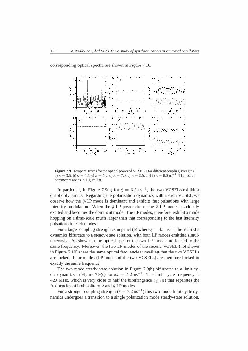
122 Mutually-coupled VCSELs: a study of synchronization in vectorial oscillators
corresponding optical spectra are shown in Figure 7.10.
Figure 7.9. Temporal traces for the optical power of VCSEL 1 for different coupling strengths.a)κ = 3.5, b)κ = 4.5, c)κ = 5.2, d)κ = 7.0, e)κ = 8.5, and f)κ = 9.0 ns−1. The rest ofparameters are as in Figure 7.8.
In particular, in Figure 7.9(a) forξ = 3.5 ns−1, the two VCSELs exhibit achaotic dynamics. Regarding the polarization dynamics within each VCSEL weobserve how they-LP mode is dominant and exhibits fast pulsations with largeintensity modulation. When they-LP power drops, thex-LP mode is suddenlyexcited and becomes the dominant mode. The LP modes, therefore, exhibit a modehopping on a time-scale much larger than that correspondingto the fast intensitypulsations in each modes.
For a larger coupling strength as in panel (b) whereξ = 4.5 ns−1, the VCSELsdynamics bifurcate to a steady-state solution, with both LPmodes emitting simul-taneously. As shown in the optical spectra the two LP-modes are locked to thesame frequency. Moreover, the two LP-modes of the second VCSEL (not shownin Figure 7.10) share the same optical frequencies unveiling that the two VCSELsare locked. Four modes (LP-modes of the two VCSELs) are therefore locked toexactly the same frequency.
The two-mode steady-state solution in Figure 7.9(b) bifurcates to a limit cy-cle dynamics in Figure 7.9(c) forxi = 5.2 ns−1. The limit cycle frequency is420 MHz, which is very close to half the birefringence (γp/π) that separates thefrequencies of both solitaryx andy LP modes.
For a stronger coupling strength (ξ = 7.2 ns−1) this two-mode limit cycle dy-namics undergoes a transition to a single polarization modesteady-state solution,

7.3 Dynamics accompanying polarization switchings 123
Figure 7.10. Optical spectra of VCSEL 1 for different coupling strengths. a) κ = 3.5, b)κ = 4.5, c)κ = 5.2, d)κ = 7.0, e)κ = 8.5, and f)κ = 9.0 ns−1. The rest of parameters areas in Figure 7.8.
Figure 7.9(d). When analyzing the bifurcation diagram of Figure 7.8, we observethat this transition seems to occur at a defined coupling strength. The bifurcationto a single polarization mode is found at the coupling where the minimum of theintensity oscillations of thex-mode becomes equal to the maximum of the oscilla-tions of they-mode. This observation hints the fact that a collision of limit cyclesmay have an influence on the polarization switching.
As we further increase the coupling strength the single polarization modesteady-state Figure 7.9(d) bifurcates to a single-mode time-periodic dynamics withfrequency close to 3.6 GHz, Figure 7.9(e), and then to a two-mode time-periodicdynamics with a slower frequency close to 2.2 GHz observed inFigure 7.9(f) forξ = 9 ns−1.
Therefore, the two-mode limit cycle dynamics exhibited in panels (c) and (f) ofFigure 7.9 even appearing for slightly different coupling strentgh values (ξ = 5.2ns−1 andξ = 9.0 ns−1, respectively) oscillate at very different frequencies, 420MHz and 2.2 GHz, respectively, what possibly indicates a different origin of theoscillations. Another interesting observation comes fromthe correlation analysisbetween both VCSELs intensities. In Figure 7.9(c) the two polarization modes inVCSEL 1 are completely in-phase with those of VCSEL 2, while in Figure 7.9(f)they are in a perfect anti-phase regime. In both cases, however, it should be noticedthat the correlation between the polarization modes withinthe same VCSEL shows

124 Mutually-coupled VCSELs: a study of synchronization in vectorial oscillators
that both modes are phase locked in an anti-phase regime. Consequently, we showthat different correlation properties between the two VCSELs (from complete in-phase to complete anti-phase) can be obtained depending on the exact value of thecoupling strength linking the dynamics of both laser oscillators.
The visualization of these simulations in the Poincare sphere provide us a com-plete picture of the polarization dynamics when increasingthe coupling strengthFigure 7.11. For small coupling strengths corresponding topanel a), we can ob-serve both lasers exhibit a chaotic polarization dynamics where the polarizationvisiting all possible sections in the Poincare sphere. Moreover, the polarizations ofthe two lasers run uncorrelated over the surface of such spehere indicating that nosynchronization is occuring between the VCSELs. In former figures we showedthat steady-states with non-zerox and y-polarization components were found forintermediate coupling strengths. In panel b) we show that such states are associ-ated to stable elliptic polarization modes instead of just to LP modes. It is alsoobserved that the slow oscillations in panels c) and f) of Figure 7.9 correspondto limit cycle orbits on the Poincare sphere, while fast oscillations in panel e) areinduced by fast changes in the total optical power with a fixedlinear polarization.
Figure 7.11. Stokes parameters in the Poincare sphere for different coupling strengths. a)κ = 3.5, b) κ = 4.5, c) κ = 5.2, d) κ = 7.0, e) κ = 8.5, and f)κ = 9.0 ns−1. Therest of parameters are as in Figure 7.8. Black and red distinguish VCSEL 1 and VCSEL 2,respectively.

7.4 Misalignment effects 125
7.4 Misalignment effects
So far all the results concerning the coupling-induced PS and the accompanyingdynamics, including the synchronization properties have been obtained assuminga perfect alignement between the eigenaxes (x andy) of both VCSELs. In this sec-tion we investigate the possible consequences of breaking up such a condition byrotating one of the VCSELs with respect to the other. This manipulation is easilyaccessible from an experimental point of view and calls for afully vectorial studyof the polarization degree of freedom.
Numerical integration of Eqs. (7.1)-(7.6) when scanning the coupling and ro-tation angle between the VCSELs leads to the output of Figure7.12. For a fixedcoupling, we notice that the effect of the rotation of a VCSELis to continuoslydecrease the power associated to one of the LP-modes while itincreases the inten-sity corresponding to the orthogonal one. For example atξ = 5 ns−1, thex-modestarts decreasing its power simultaneously in VCSELs 1 and 2, while they-modegradually increments its power in both lasers. This tendency is maintained untilthe rotation angle becomes a bit larger than one quarter of revolution θ = π/2 forwhich the power of they-mode reaches its maximum and thex-mode its minimumvalue. From that point, the recovery of the initial values finishes atθ = π, i.e., halfa revolution of one of the VCSELs, demonstrating that the system is invariant toan upside-down turning of one of the VCSELs.
Figure 7.12, although indicating that there is a transfer ofpower between thexandy linearly polarized projections, it does not capture how this transition occurs.In the following we analyze the evolution of the components of the polarizationvector of both VCSELs as a function of the rotation angleθ.
The four Stokes parameters are represented in Figure 7.13 for the polarizationof both VCSELs when we rotate one of the VCSELs. In Figure 7.13(a) the evolu-tion ofS0, which represents the total intensity of light, indicates that upon rotationof one of the VCSELs the total power emitted remains constantand identical inboth VCSELs except for a tiny window where the intensity becomes chaotic. Panelb) of Figure 7.13 demonstrates that the projection of the vector of polarization ontheS1 axis is the same for the two lasers. This projection decreases from its maxi-mum attained atθ = 0 andπ down to zero for values ofθ slightly larger thanπ/2and3π/2. Regarding theS2 andS3 components, in panels c) and d) it is observedthat the two VCSELs always exhibit an opposite sign for theS2 andS3 projectionsof their respective polarization vectors.
Two key features are remarkable in Figure 7.13. One comes from the obser-vation thatS3 is in general different from zero for most of the values ofθ. Thisfact yields to stable elliptic polarization states of lightin our coupled configurationwhich moreover can be induced by a pure mechanical operation, i.e., by rotatingone of the lasers. One must remind that such states are not usually found to be sta-

126 Mutually-coupled VCSELs: a study of synchronization in vectorial oscillators
Figure 7.12. Time-averaged intensities in thex- and y-LP modes of VCSEL 1 and 2 as afunction ofξ andθ. Parameters are specified in Table 7.1.
ble in solitary VCSELs. A second attracting characteristicis related to the suddenjumps in theS2 andS3 components of the polarization vectors found for values ofthe rotation angle nearθ ∼ π/2 and∼ 3π/2. Thus, when crossing one of thesecritical angles the polarization state of the VCSELs suffers the sharp transition(S0, S1, S2, S3) 7−→ (S0, S1,−S2,−S3). These jumps correspond to an inversionof the polarization vector on theS1 axis, occuring when one of the VCSELs is ro-tated by approximately half a revolution respect to the other laser. Near the criticalangles ofθ = π/2 and3π/2 we found thatS1 ∼ 0 andS3 is small compared toS2. Consequently, the abrupt inversion of the sign ofS2 for those angles can bethought as a sharp transition from a−45 to a+45 quasi-linearly-polarized emis-sion of light in VCSEL 1, and the opposite transition for VCSEL 2.
We have also shown in Figure 7.14 that by reversing the rotation angle (i.e.,turning the same VCSEL in the opposite sense) the sharp polarization switchingsoccur at similar but slightly different angles. Thus, if by increasing the rotationangle the first PS occurs atθ ∼ 103 when rotating the laser in the other sense thePS appear atθ ∼ 75. This difference provides a clear hysteresis spanning more

7.4 Misalignment effects 127
Figure 7.13. Stokes parameters evolution of the light emitted by the two VCSELs as a functionof the rotation angle. Black and red traces represent the Stokes components of the VCSEL 1and 2 polarization vectors, respectively. The coupling strength is fixed toξ = 10 ns−1.
Figure 7.14. Stokes parameters evolution of the light emitted by the two VCSELs whendecreasing the rotation angle. Black and red traces represent the Stokes components of theVCSEL 1 and 2 polarization vectors, respectively. The coupling strength is fixed toξ = 10ns−1.

128 Mutually-coupled VCSELs: a study of synchronization in vectorial oscillators
than 30 angular degrees around the values ofθ = 90 andθ = 270.
Figure 7.15 contains the evolution of the Stokes parameterson the Poincaresphere for increasing and decreasing the angle of rotation.In such a representation,the PS and hysteresis effects are evident.
Figure 7.15. Stokes parameters evolution on the Poincare sphere of the light emitted by thetwo VCSELs when increasing and decreasing the rotation angle; a) VCSEL 1 increasingθ, b)VCSEL 2 increasingθ, c) VCSEL 1 decreasingθ, and d) VCSEL 2 decreasingθ. Black andred distinguish VCSEL 1 and VCSEL 2, respectively. The arrows indicate the sharp transitionswhen varying the rotation angle.
Thus, in conclusion we have first described how the mechanical rotation of oneof the devices around the critical angles can be optically encoded by the macro-scopic polarization state of light of the VCSELs, and secondhow the bistabilityfound around such PS also permits to detect and record the sense of the inducedrotation.

7.5 Synchronization 129
7.5 Synchronization
In Section 7.3, we have reported that two mutually-coupled VCSELs can oscillatein regimes of periodic in-phase or anti-phase dynamics. There, the transition fromone to another solution was induced by varying the interaction strengthξ. How-ever, in those cases the cavity anisotropies induce that thetwo eigenaxesx andyare favored directions of the polarization state, thus imposing serious constraintsto the vectorial nature of the synchronization scenario.
Here, in order to investigate the synchronization properties between the com-plete polarization vectors of two VCSELs we assume that the anisotropies of bothlaser cavities are negligible. By doing so we achieve to relax the preference ofthe VCSELs to emitt light polarized along some definite directions. In such con-ditions the fundamental question to be answered is how the polarization vector ofeach VCSEL is going to evolve?
First we analyze the situation corresponding to a solitary VCSEL. In the puredeterministic case it is observed that all the linearly polarized states are equivalentand neutrally stable. Consequently, there is no preferencefor a particular stateand depending on the initial condition the polarization vector settles on a givendirection. In the presence of spontaneous emission noise, the polarization vectorof each solitary VCSEL is found to diffuse around the equatorof the Poincaresphere, i.e., to perform a random walk visiting all the possible linearly polarizedstates.
Panel a) in Figure 7.16 shows the polarization vectors of twoVCSELs whenthey are uncoupled and free from anisotropies. Clearly, both vectors diffuse with-out any correlation between each other. For low coupling rates such in panel b),a kind of synchronization must occur between both polarization vectors becausenow they scan at the same time the same Poincare sphere region. For intermediatecouplings (panel c)) one finds a region of chaotic states where the polarization vec-tors visit all the sphere surface, while for larger interaction strengthsξ ≥ 7 ns−1
both vectorial oscillators diffuse again around the equator. We have also noticedthat the larger the coupling strength the smaller the area ofthe Poincare sphere thatis visited in the same time.
Now, we can study whether such random walks can synchronize.Figure 7.17(left panel) shows the maxima of the cross-correlation functions between theStokes parameters of both lasers as a function of the coupling strength. Remark-ably, both polarization vectors continue to diffuse mainlyaround the equator ofthe Poincare sphere driven by independent spontaneous noise sources and nev-ertheless, a large correlation value is found between the dynamics of the threecomponents of both polarization vectors. The effect of the time delay in the in-teraction between the VCSELs is reflected in the timing of thesynchronizationof the polarization dynamics. Figure 7.17 (right panel) plots the lag at which the

130 Mutually-coupled VCSELs: a study of synchronization in vectorial oscillators
Figure 7.16. Stokes parameters evolution on the Poincare sphere of the light emitted by thetwo VCSELs for different values of the coupling strength; a)ξ = 0 ns−1, b) ξ = 2 ns−1,c) ξ = 4 ns−1, and d)ξ = 20 ns−1. Black and red distinguish VCSEL 1 and VCSEL 2,respectively.

7.6 Conclusions 131
maximum of the cross-correlation function between the two polarization vectors isattained. For most of the coupling values the cross-correlation function is almostsymmetric around zero with two similar maxima at±τ . This fact is reflected inFigure 7.17 where for large coupling rates the lag randomly fluctuates between200 ps and−200 ps, i.e., the coupling time.
Figure 7.17. Left: maxima of the cross-correlation functions between the polarization compo-nents of both VCSELs as a function of the coupling strength. Right: lag at which the maximaof the cross-correlations are found as a function of the coupling strength.
7.6 Conclusions
In this chapter we have shown that mutual coupling may inducemultiple bistablepolarization switchings in otherwise polarization stableVCSELs.
A sequence of PS events has been found when varying the coupling strengthor the propagation phase between the VCSELs. The definite periodicity of thesePS events has been related to the creation of new compound-cavity modes withhigher gain and orthogonal polarization. Each PS is accompanied by a large hys-teresis whose width can be tuned by the coupling parameters.Such controllablebistable PS system is interesting for fast optical switching applications. We havealso checked that this coupling-induced PS scenario is robust against modificationsof the corresponding laser and coupling parameters.

132 Mutually-coupled VCSELs: a study of synchronization in vectorial oscillators
Moreover, the effect of a detuning between the lasers free-running optical fre-quencies has been found to induce another type of PS.
Stable elliptic polarization states are achieved by the rotation of one of theVCSEL respect to the other. This situation is also responsible for the appearanceof sharp jumps in some components of the polarization vectorof each VCSEL.
Finally, we have observed the temporal synchronization of the polarizationvectors of isotropic VCSELs. Thus, a true vectorial synchronization in mutually-coupled VCSELs has been numerically demonstrated.

Chapter 8
Synchronization of threemutually-coupledsemiconductor lasers
EXPERIMENTS1 and numerical simulations have demonstrated that the coupling-induced dynamics of two semiconductor lasers interacting through the mutual
injection of their coherent optical fields exhibit a symmetry breaking [10, 12]. In-stead of showing an identical behavior, spontaneously, thetwo twin lasers de-velop an achronal generalized synchronization between them. This type of syncis mainly characterized by peaks at±τ , with τ being the coupling time, in thecross-correlation function between the lasers intensities.
From a different perspective, investigations of three instantaneously-coupledsemiconductor or solid-state lasers interacting through their overlapping opticalfields were performed by Winful et al. [16], and Roy and collaborators [17]. Theseauthors observed that when arranged in a linear array, a identical synchronizationbetween the first and third lasers showed up, while the temporal traces of any ofthe extreme lasers and the central one appeared rather uncorrelated.
These interesting results motivate a deeper study on how thenumber of lasersand the network of couplings modify the synchronization properties of SLs inter-acting with a finite time delay. New questions need to be addressed. For instance,can the isochronous solution between the first and third lasers be maintained evenwhen the lasers need a time to communicate? How will the sync look like if weadd a fourth laser to the array? What is the role of the symmetry on selectingpossible sync patterns? With a view to answer these questions, we study here the
1This chapter is based on the paper: “Zero-lag long-range synchronization via dynamical relay-ing” by I. Fischer, R. Vicente, J. Buldu, M. Peil, C.R. Mirasso, M.C. Torrent, and J. Garcia-Ojalvo,to appear in Physical Review Letters (2006)
133

134 Synchronization of three mutually-coupled semiconductorlasers
synchronization properties of semiconductor lasers arranged in open-end (linearchain) and ring configurations. Arrays up to six SLs have beenexplicitely an-alyzed. Symmetry arguments support the opinion that the patterns of solutionsfound for arrays of those size are maintained for larger number of units.
After introducing the modeling equations and parameters, we present our mainresults in Section 8.2. There we focus on the open-end configuration of threemutually-coupled SLs. In particular, we show that zero-lagsynchronization be-tween the extreme lasers in an open-end configuration can be achieved by relayingthe dynamics via the central laser, which surprisingly lagsbehind the synchro-nized outer elements. The characterization of the coupling-induced instabilitiesand their robustness are also analyzed there. Subsequent sections are devoted tothe effect of increasing the number of laser elements in boththe open-end andring configurations. The role of the symmetry and delay in restricting the possiblesynchronization spatial profiles is also explained there. Aconnection between thechaotic synchronization solutions and the time-periodic patterns of oscillation isproposed. Finally, zero-lag synchronization between distant coupled lasers is usedto propose a new chaotic communication scheme in Section 8.4. Conclusions aresummarized in Section 8.5 where the experimental confirmation by the groups ofDarmstadt and Terrassa of the zero-lag sync in a laser setup is also briefly com-mented.
8.1 Model
The system under investigation consists of single-mode SLscoupled via the de-layed mutual injection of their lasing modes in a given network of connections.For numerical purposes the modeling is performed at the level of rate equationsaccording to Ref. [98], which take into account the different delayed couplingterms between the SLs.
Figure 8.1. Open-end scheme of three mutually-coupled semiconductor lasers interactingwith a time delay.
The adaptation of such a modeling to the case of three mutually-coupled SLsinteracting in an open-end configuration (as sketched in Figure 8.1) reads

8.1 Model 135
E1 = i∆ω1E1 +1
2(1 + iα)G(N1, ‖E1‖)E1
+ κ21 exp(iφ21)E2(t− τ21) (8.1)
N1 =I1e
− γeN1 −G(N1, ‖E1‖)‖E1‖2 (8.2)
E2 = i∆ω2E2 +1
2(1 + iα)G(N2, ‖E2‖)E2
+ κ12 exp(iφ12)E1(t− τ12) + κ32 exp(iφ32)E3(t− τ32) (8.3)
N2 =I2e
− γeN2 −G(N2, ‖E2‖)‖E2‖2 (8.4)
E3 = i∆ω3E3 +1
2(1 + iα)G(N3, ‖E3‖)E3
+ κ23 exp(iφ23)E2(t− τ23) (8.5)
N3 =I3e
− γeN3 −G(N3, ‖E3‖)‖E3‖2 , (8.6)
whereEm(t) is the complex amplitude of the optical field generated by lasermandNm represents the corresponding carrier number.‖ · · · ‖ denotes the amplitudeof the complex field. The nonlinear gain functionG(Nm, ‖Em‖2) is given by:
G(Nm, ‖Em‖) ≡ g(Nm −No)
1 + s‖Em‖2− γ .
The coupling parameters that define the interaction betweenany two lasers aregiven by the coupling weight[κmn], the coupling time[τmn], and the couplingphase[φnm] = Ω[τmn] mod 2π matrices. Thus, in the case of a general networkthe equations defining the interaction between lasers are written as
Em = i∆ωmEm +1
2(1 + iα)G(Nm, ‖Em‖)Em
+∑
n 6=m
κnm exp(iφnm)En(t− τnm) (8.7)
Nm =Ime
− γeNm −G(Nm, ‖Em‖)‖Em‖2 (8.8)

136 Synchronization of three mutually-coupled semiconductorlasers
8.2 Dynamics of three semiconductor lasers in an open-end configuration
In the subsequent sections we focus first on the open-end configuration of threemutually-coupled SLs. The internal laser parameters are assumed identical for thethree lasers; the linewidth enhancement factorα = 3, the differential gaing =1.2 × 10⁻⁵ ns−1, the transparency value for the carrier numberN0 = 1.25 × 10⁸,the saturation coefficients = 5 × 10⁻⁷, the photon decay rateγ = 496 ns−1,and the carrier decay rateγe = 0.651 ns−1. With these internal parameters thethreshold current of the three lasers isIth = 17.35 mA. In the former equations,the reference frequency for the slowly-varying amplitude of the electric fields ischosen to beΩ = (ω1 + ω2 + ω3)/3, whereωi is the central frequency of eachsolitary laser. Detunings (∆ωi) are taken with respect toΩ. Unless other couplingconditions are explicitly mentioned in the text the coupling strengths, delay times,and propagation phases are assumed to be identical in the twocoupling branchesof Figure 8.1;κ1,2 = κ2,1 = κ3,2 = κ2,3 = 20 ns−1, τ1,2 = τ2,1 = τ3,2 = τ2,3 =3.65 ns, andφ1,2 = φ2,1 = φ3,2 = φ2,3 = 0 rad.
8.2.1 Coupling-induced instabilities
In order to explore the instabilities emerging from the mutual coupling of threesemiconductor lasers interacting with a time delay, we firstset the lasers to op-erate in a highly symmetric configuration namely, within a perfect free-runningfrequency tuning (∆ω1 = ∆ω2 = ∆ω3 = 0) and a moderate and identical currentpump I = I1 = I2 = I3 = 27.5 mA. With this level of pumping the solitaryrelaxation oscillation frequency of the three lasers amount to 4.33 GHz.
Once coupled under standard conditions the three semiconductor lasers areobserved to enter into a fully chaotic regime known as Coherence Collapse (CC).Remarkably, after some transient the traces of the outer lasers, i.e., SL1 and SL3,start to become more and more alike up to the point that they end up being per-fectly synchronized at zero-lag. The numerical results areshown in Figure 8.2. Inorder to check the robustness of this synchronization phenomena we have simu-lated Eqs. (8.1)-(8.6) starting from various and non-identical initial conditions forthe lasers. All the simulations returned the same results; the zero-lag synchroniza-tion of the lasers occupying the extreme positions in the array. At this point it isworth to remember that the symmetry under the exchange between lasers 1 and3 only assures the existence of the synchronized solution but not its stability. Ofcourse, in this zero-lag synchronization no superluminal effect is taking place, butthis is another example of self-organizing dynamics where the units composing thesystem negotiate a complex and unexpected behavior.
Moreover, the computation of the cross-correlation functions between thelasers reveals a high degree of similarity between any of theouter laser traces

8.2 Dynamics of three semiconductor lasers in an open-end configuration 137
Figure 8.2. Temporal traces of the open-end configuration with three lasers. κ = 20 ns−1
andτ = 3.65 ns.
and the central one. In Figure 8.3 it is observed that once properly shifted a highdegree of correlation (∼ 0.8) appears between the traces of any of the extremelasers and the laser 2. In this case, however, the lag for which the maximum of thecross-correlation function appears corresponds to the coupling time. The asym-metric cross-correlation function between SL1 (or SL3), and SL2 signals that theouter lasers are advancing the dynamics of the central one bya time delayτ . Sur-prisingly, the mediator element is lagging behind the synchronized outer units forwhich it is acting as a communicating bridge. This type of dynamics excludes theinterpretation of the central element as a simple leader directly forcing the extremelasers.
Figure 8.3. Cross-correlation functions for the open-end configuration with three lasers.κ =20 ns−1 andτ = 3.65 ns.
Interaction strength effect
How this synchronization scenario depends on the strength of the interaction be-tween lasers is investigated next. To this end, we adiabatically increase the cou-pling strength between the three SLs and record a time seriesfor each value of thecoupling rate. The common coupling strengthκ = κ12 = κ21 = κ23 = κ32 isvaried from 0 ns−1 to 30 ns−1. The common coupling delay time is maintainedconstant atτ = 3.65 ns. For each time series, we compute the cross-correlationfunction between pairs of lasers and the lag for which the maximum of this func-

138 Synchronization of three mutually-coupled semiconductorlasers
tion appears. The correspoinding results are shown in Figure 8.4. For most of thecoupling strength values the three lasers are operated in the chaotic CC regime.Nevertheless, some windows of periodic behavior are also observed for small cou-pling rates. Interestingly, regardless the dynamics exhibited by the lasers, the per-fect synchronization at zero-lag between the extreme unitsextends to all the cou-pling values explored. No coupling threshold for the transition from unsynchro-nized to synchronous motion can be observed for this pair of lasers which achievethe sync state for arbitrarily small couplings. The centrallaser, on the other hand,varies its correlation coefficient with the outer units froma value of1 obtained forsmall couplings and periodic dynamics to a value around∼ 0.8 attained for largestrengths where chaotic dynamics develops. From coupling ratesκ & 6 ns−1 thelag between SL2 and SL1 (or SL3) stabilizes aroundτ . The fluctuations in the lagvalue for small coupling strengths can be associated to the high symmetry of thecross-correlation functions that appear for regular dynamics stages.
Figure 8.4. Cross-correlation and lag between pairs of SLs as a functionof their commoncoupling strengthκ.
The transition from the two-laser problem
To better understand the link from the two-coupled lasers problem to our casewith three interacting lasers, we performed the following numerical experiment.Now, instead of symmetrically increasing the coupling strength between the threelasers, we start from a configuration where only SL1 and SL2 are interacting with

8.2 Dynamics of three semiconductor lasers in an open-end configuration 139
a constant coupling strength (κ12 = κ21 = 20 ns−1). Laser 3 is put into play bycontinously increasing the coupling ratesκ23 = κ32 from 0 ns−1 to 30 ns−1. InFigure 8.5 we can appreciate the cross-correlation and lag analysis.
Figure 8.5. Cross-correlation and lag between the pairs of SLs as a function of the couplingstrength between SL2 and Sl3 (κ23 = κ32).
We observe that the cross-correlation function between theouter lasers grows asthe coupling strength is varied up to the value whereκ23 = κ32 = 20 ns−1, forwhich the degree of sync is maximum. The lag between SL1 and SL3 is again zerofor most of the coupling rates investigated. The synchronization quality betweenany of the extreme lasers and the central one continously grows to exhibit a peak atκ23 = κ32 = 20 ns−1. After that point, the correlation between SL1 and SL2 startsto decrease, while the sync between lasers2 and 3 is maintained almost constant ata value around∼ 0.7. It is interesting to note that for example atκ23 = κ32 = 30ns−1, the interaction between lasers 2 an 3 is stronger than when the coupling isset atκ23 = κ32 = 20 ns−1, and nevertheless, the sync between these two lasersis better in this last case due to symmetry reasons. Regarding the lag analysis, weobserve that for moderate to large coupling values (& 10 ns−1) both extreme lasersadvance the dynamics of the central one by a timeτ .
So far we have only considered symmetric mutual interactions between anypair of lasers. This is, for any pair of lasers(n,m) the coupling strength wassuch thatκnm = κmn. Keeping this situation, it is clear that the central laser is al-ways receiving more optical injection than the outer ones because it is the only onelinked to two lasers simultaneously. To check whether the synchronization solu-

140 Synchronization of three mutually-coupled semiconductorlasers
tions we have observed until now are maintained when reversing this situation, i.e.,SL2 receiving less optical injection than SL1 and SL3, we perform the followingnumerical simulations. We fix the coupling strengths from SL2 to the outer lasersatκ21 = κ23 = 20 ns−1, and scan the input coupling of SL2 fromκ12 = κ32 = 0ns−1 up to30 ns−1. The correlation analysis is presented in Figure 8.6.
Figure 8.6. Cross-correlation and lag between the pairs of SLs as a function of the centrallaser input strength (κ12 = κ32).
Under these conditions the synchronization between the extreme lasers at zero-lag is still a compatible state of the system Eqs. (8.1)-(8.6), and it appears to bestable in all the range of coupling strengths investigated.Regarding the leader-laggard role between any of the extreme lasers and the central one, there is a clearchange of tendency occurring atκ12 = κ32 ∼ 10 ns−1. We first analyze thecase for coupling strengths below such a critical rate. There, the cross-correlationfunction between any of the extreme lasers and SL2 typicallyshows two peaks at±τ . However, in such functions the peak associated to the situation in which thecentral laser advances the extreme ones is only a little bit higher than the other peakwhich is related to the opposite situation. Since the difference between the twopeaks is very small, it is difficult then to speak about a leader-laggard dynamics.On the contrary, for coupling strengths above∼ 10 ns−1, the difference betweenpeaks is now much larger than in the previous case, and hence indicates a clearlydefined leader-laggard dynamics. For this large coupling regime, the dynamics ofthe extreme lasers is always found to advance the central oneby an injection delaytime τ .

8.2 Dynamics of three semiconductor lasers in an open-end configuration 141
8.2.2 Robustness of the synchronization solution
Natural detuning
The ability exhibited by a set oscillators to synchronize isstrongly dependenton how far their natural frequencies are. This characteristic naturally leads tothe concept of Arnold tongue, which has been already studiedin Chapter 6 foroptoelectronically-interacting lasers. Moreover, the role of a moderate detun-ing between the free-running optical frequencies of two coherently-coupled edge-emitting lasers has been found to establish a leader-laggard role, with the high-frequency laser advancing the dynamics of its counterpart [10, 12]. Since a smalldetuning is almost unavoidable in real experiments, we havestrong motivations toinvestigate here what the effects of a small detuning between the different lasers inour open-end scheme are.
We first recover the standard coupling conditions by settingall the couplingconstants atκ = κ12 = κ21 = κ23 = κ32 = 20 ns−1, and the delay times atτ = τ12 = τ21 = τ23 = τ32 = 3.65 ns.
We start with the case where the outer lasers share a common solitary fre-quency (∆ω1 = ∆ω3 = 0) and we only allow for a detuning with respect to thecentral laser (∆ω2 6= 0). The central laser frequency detuning is scanned from−22.5 GHz up to22.5 GHz in Figure 8.7. The graphics show that the zero-lagsynchronization between SL1 and SL3 is perfectly maintained in all the range ofvalues considered for the detuning. In most cases, both extreme lasers advancethe dynamics of the central one and only for very high positive detunings this lagchanges its sign. However, looking in more detail at this hypothetical reversalof the leader-laggard role we must notice that it occurs for avalue of the detun-ing where the synchronization between the central and extreme lasers is almostlost (at∆ω2 = 18 GHz the maximum of correlation is∼ 0.2). In fact, around±τ the cross-correlation function also presents two negativepeaks reaching thevalue of∼ −0.5, and hence, indicating that actually an anticorrelated dynamicsbetween the central and the outer lasers is taking place. Theobservation of thisantisynchronization regime can be related to the properties of a laser injected by afield largely detuned from its cavity resonance. The key point is that this type ofinjection produces an incoherent interaction where the injecting field suppressesthe gain function of the laser by consuming carriers that cannot be devoted to itsown lasing action. Thus, a fluctuation in the amplitude of theinjecting field isassociated with a variation of the laser power with an opposite sign.
If a detuning occurs between the extreme units (∆ω1 − ∆ω3 6= 0), we havenumerically checked that the qualitative features of the solution obtained for theperfectly symmetric case are preserved to some extend. The robustness of theisochronal sync between SL1 and SL3 is observed to amount to afew Gigahertz

142 Synchronization of three mutually-coupled semiconductorlasers
Figure 8.7. Cross-correlation and lag between the pairs of SLs as a function of the centrallaser frequency deviation,∆ω2.
(see Figure 8.8). The relative dynamics, i.e., the leader-laggard role, between thethree lasers outside the zero-detuning point becomes difficult to interpret since thecorrelation coefficient drops very fast down to zero.
Figure 8.8. Cross-correlation and lag between the pairs of SLs as a function of the detuningbetween the extreme lasers (∆ω1 − ∆ω3).

8.2 Dynamics of three semiconductor lasers in an open-end configuration 143
Pumping mismatch
Even if the electrical current injected into the active layer of a semiconductorlaser can be very well controlled at the experimental level,it is still very inter-esting to check the stability of the synchronization solution upon current mis-matches between the coupled lasers. Moreover, different dynamical regimes andsynchronization characteristics only appear at certain injection current rates. Forthis reasons in this section we evaluate the effect of considering different pump-ing levels for each laser and we check the robustness of the synchronization so-lution. As in the previous study of the detuning effect, the coupling strengthsare fixed atκ12 = κ21 = κ23 = κ32 = 20 ns−1, and the delay times atτ12 = τ21 = τ23 = τ32 = 3.65 ns.
We first proceed by varying the bias current of the central laser I2 from 17.5mA to 37.5 mA, while keeping the extreme laser pumps constantat I1 = I3 =27.5 mA. As we observe from Figure 8.9 the only effect of increasing I2 is tomonotonically decrease the synchronization level betweenthe extreme lasers andthe central one. However, the degradation of the sync quality is not severe and thecorrelation coefficient only decreases from almost1 down to∼ 0.7 when varyingthe pump current of the central laser by more than 20 mA. It is worth noting thatthe maximum of the correlation between SL2 and SL1 or SL3, is not attained inthe symmetric configuration where all three lasers are operating at 27.5 mA butat pump levels of the central laser close to the threshold. These results togetherFigure 8.4 are indicative of the very low optical power that is needed to bring theouter elements SL1 and SL3 into synchrony.
Regarding the timing of the synchronized solutions it is observed that the lagsat which the maxima of the cross-correlation functions appear do not shift with thepump level.
One can also consider pump mismatches between the lasers occupying theextreme positions, i.e., SL1 and SL3. We observe how the effects on the synchro-nization are much more severe now. The results are summarized in Figure 8.10where the bias current of SL3 is scanned from 17.5 mA to 37.5 mA. The levels ofSL1 and SL2 are fixed to 27.5 mA. In this case the sync between the outer lasers isonly maintained for a range a few miliamperes wide. For smallpump deviations,series of bursts of desynchronization perturb the generalized synchronization so-lution between SL1 and SL3.
Pulse propagation
In the former subsections we have demonstrated that the synchronization betweenthe extreme lasers is only moderately robust against a mismatch between them. Onthe other hand, the effect of mismatches between the centrallaser and the extreme

144 Synchronization of three mutually-coupled semiconductorlasers
Figure 8.9. Cross-correlation and lag between the pairs of SLs as a function of the currentlevel of the central laser.
Figure 8.10. Cross-correlation and lag between the pairs of SLs as a function of the currentlevel of laser 3.

8.2 Dynamics of three semiconductor lasers in an open-end configuration 145
units turned out to be hardly significant and the synchronization between SL1 andSL3 was found to be extremely robust upon changes in the parameters of centrallaser.
These results have been obtained under the conditions of stationary mis-matches, i.e., once the differences in the natural frequencies or pumping levelswere set they were kept constant along the temporal evolution of the lasers. Here,we investigate the effects of a dynamical perturbation on the synchronization pat-tern that we have previously reported. In particular, we generate a pulse of currentin one of the lasers and study how this perturbation propagates in the system andaffects the synchronization solutions.
Within the standard and symmetrical coupling conditions, we start by gener-ating in the central laser a current pulse of Gaussian profilewith amplitude 10mA and full width at half maximum (FWHM) of 1.2 ns. The time series of thethree lasers, the pulse profile, and the synchronization error and sync plot for SL1and SL3 are all collected in Figure 8.11. The synchronization solution betweenthe extreme lasers is perfectly maintained, even at the moment in which the per-turbation reaches the lasers SL1 and SL3, one coupling time after the pulse wasgenerated. We see then that the perturbation remains completely unnoticed fromthe synchronization point of view.
Figure 8.11. Top: temporal traces of the optical power of the three lasers. Bottom: pulsewaveform, sync error and sync plot between lasers 1 and 3.
If the same pulse is now generated in one of the lasers occupying the extremepositions, Figure 8.12 clearly shows that the sync error between lasers 1 and 3

146 Synchronization of three mutually-coupled semiconductorlasers
becomes different from zero only during the pulse generation. This means thatimmediately after the perturbation on SL1 ends, even still traveling through thesystem, it has no more effects on the synchronization solution. This result stronglysuggests that once the perturbation reaches the central laser, it is symmetricallydistributed toward SL1 and SL3. Otherwise, replicas of the original disturbance inthe synchronization error would be expected for time2τ and multiples of it, afterthe pulse generation.
Figure 8.12. Top: temporal traces of the optical power of the three lasers. Bottom: pulsewaveform, sync error and sync plot between lasers 1 and 3.
In cases where the amplitude of the pulses was increased up to50 mA (notethat this value is almost double than the bias current level)or the width of thepulse enlarged up to 12 ns (a value much larger than the coupling delay time),the same phenomena were found. Hence, the sync between lasers is proven tobe quite stable under dynamical perturbations pushing awaythe solution from thesynchronization manifold.
8.2.3 Synchronization for asymmetric coupling times
So far, we have taken both branches of the network module in Figure 8.1 to beidentical and to give rise to the same coupling times. But, will synchronizationexist and be stable if different lengths for the paths between lasers are considered?
To test this interesting scenario we set the coupling delay times in bothbranches to be very different. We chooseτa = τ12 = τ21 = 12 ns and

8.2 Dynamics of three semiconductor lasers in an open-end configuration 147
τb = τ23 = τ32 = 3 ns. For moderate coupling strengths, now the synchro-nization between SL1 and SL3 appears when comparingP1(t) with P3(t + ∆τ),where∆τ = τb − τa. This is, the outer laser of the shortest branch (in this caseSL3) is able to advance the behavior of the other one (SL1), which is more than 15ns apart, by the difference of coupling times.
As we have done before the stability of this solution can be checked by subject-ing the central laser to a given perturbation. A Gaussian pulse of current is againchosen to test the robustness of the solution. Figure 8.13 shows the temporal tracesof the three lasers, the pulse generated in SL2, and the synchronization error andsync plot between SL1 and SL3 once the corresponding shift (∆τ = τb − τa) hasbeen compensated for. The temporal traces already demonstrate the timing of thesynchronization solutions, where SL3 clearly advances thebehavior of SL1. Thesynchronization plots show that within our numerical precision the lagged syn-chronization here attained is a perfect solution, not even affected by a perturbationin the element mediating the synchronization.
Figure 8.13. Top: temporal traces of the optical power of the three lasers. Bottom: pulsewaveform, sync error and sync plot between lasers 1 and 3.τa = τ12 = τ21 = 12 ns andτb = τ23 = τ32 = 3 ns. The coupling strength is fixed toκ = 20 ns−1.
Other sets of values for the coupling times have been tested (such asτa =τ12 = τ21 = 5 ns andτb = τ23 = τ32 = 0.2 ns) and in all cases a synchronizationsolution with lagτb − τa have been obtained between SL1 and SL3. Note that inthe later case, without the presence of a third laser the pairs of mutually-coupledlasers(1, 2) and(2, 3) would exhibit very different dynamics due to the disparityin the coupling times. Nevertheless, when all three are coupled lasers 1 and 3 are

148 Synchronization of three mutually-coupled semiconductorlasers
able to perfectly synchronize.
In general, the cross-correlation function between pairs of lasers shows severalpeaks related to the delay times and their differences. Figure 8.14 contains thecross-correlation function for the three pairs of lasers(1, 2), (2, 3), and(3, 1) whenτa = 1.5 ns andτb = 3.6 ns. Different delay values have been simulated and inall cases the main peaks of the cross-correlation functionsappeared at the lags:(τa,−τa, 2τb − τa) for the pair of lasers(1, 2), (τb,−τb, τb − 2τa) for the lasers(2, 3), and (τb − τa) for the pair composed of the extreme lasers 3 and 1.
Figure 8.14. Cross-correlation functions between pairs of lasers with different coupling times.τa = 1.5 ns andτb = 3.6 ns. The coupling strength is fixed toκ = 20 ns−1.
8.2.4 Synchronization of semiconductor lasers with feedback
In the previous sections we have approached the study of the entrainment prop-erties of three mutually-coupled semiconductor lasers in alinear array. We mustnotice that before coupling them the stand-alone lasers emit CW optical power. Tosee whether synchronization occurs when each laser develops its own dynamics,we consider in this section the situation where at least the outer lasers in the arrayproduce their own instabilities before being coupled.
To this end, we add an optical feedback loop to SL1 and SL3 and fix the feed-

8.2 Dynamics of three semiconductor lasers in an open-end configuration 149
back strength and delay times to values for which these lasers enter into a chaoticdynamics when uncoupled, known as Low Frequency Fluctuations (LFF). Wereach this regime by setting the bias current very close to the thresholdI = 17.5mA, the feedback strength to 10 ns−1, and the feedback delay time to3.4 ns. Be-fore switching on the coupling, both extreme lasers oscillate chaotically in the LFFregime, but their traces are completely uncorrelated. After activating the mutual in-teractions (κ12 = κ21 = κ23 = κ32 = 20 ns−1 andτ12 = τ21 = τ23 = τ32 = 3.65ns), the LFF dynamics of both lasers exhibit a very good synchronization at zero-lag. Figure 8.15 shows the temporal traces and the cross-correlation functionsbetween the three lasers after being coupled. The lags of thesynchronization solu-tions, and consequently the leader-laggard roles between the lasers, are in generalsimilar to those obtained without feedback. However, we should notice an im-portant difference with the former case. In the presence of feedback there exists afinite coupling strength below which the dynamics of the extreme laser cannot syn-chronize. The value of this threshold is found to be very sensitive to the strengthof the feedback, the feedback round-trip time, and the bias current.
Figure 8.15. Top: temporal traces. Middle: zoomed-in filtered temporal traces. Bottom:cross-correlation function of the three lasers scheme. Lasers 1 and 3 subject to moderatefeedback,κf = 10 ns−1 andτf = 3.4 ns. The bias of all three lasers is set toI = 17.5 mA.

150 Synchronization of three mutually-coupled semiconductorlasers
8.3 The role of network on the synchronization properties
The profound qualitative changes observed when comparing the synchronizationproperties between two and three mutually-coupled lasers,strongly suggest us toproceed our investigation by including a larger number of lasers in the array. Themain goal here is to answer the question of how the synchronization characteristicsdepend on the number of lasers and the network of connectionsin a system withdelayed interactions? Two different topologies are considered for such a study,namely the open-end array and the ring configuration.
8.3.1 Open-end arrays
In the following, we present our results concerning the synchronization patternsacross the elements of an open-end array composed of four, five, and six semicon-ductor lasers. In all cases, the coupling strength between neighbor lasers is fixedto κnm = κmn = 20 ns−1 except for the six lasers setup where the strength is in-creased up to 40 ns−1. In this case, we observed that a higher coupling is requiredin order to excite instabilities in the system and study synchronization phenomena.The coupling times between adjacent lasers are adjusted toτnm = τmn = 3.65ns for all the configurations and the current bias is set toI = 17.5 mA. Undersuch conditions once coupled the lasers develop a chaotic LFF dynamics. Fig-ures [8.16-8.18] contain the temporal traces and cross-correlation analysis for allpairs of lasers in the case of 4, 5, or 6 semiconductor lasers,respectively. For con-ceptual convenience we discuss the results for different number of units altogether.
The correlation functions clearly indicate that zero-lag synchronization ap-pears between second-neighbor lasers in the array, i.e., between pairs of lasersoccupying positionsm-th andm+ 2-th. Moreover, the cross-correlation analysisalso reveals that adjacent neighbors exhibit a high degree of similarity once thetemporal series of one laser is shifted forward or backwardsa coupling timeτ .
Thus, in the open-end scheme we find that the lasers isochronously synchro-nize within two clusters; one group is defined by the lasers placed in the odd posi-tions of the linear array (SL1, SL3, SL5, · · · ) while the other assemble is composedby the lasers located at even positions (SL2, SL4, SL6, · · · ). Any pair of lasers be-longing to different clusters exhibits achronal generalized synchronization and itscross-correlation function displays two peaks at±τ , as in the original two-laserproblem. It is also noticeable by the asymmetry of some cross-correlation func-tions that the lasers occupying the outer positions of the array advance the dynam-ics of their inner neighbors. Numerical simulations with different initial conditionssupport the generality of these results for arrays of different lengths.

8.3 The role of network on the synchronization properties 151
Figure 8.16. Synchronization in a 4-lasers open-end array. Top: Lasers configuration; Middle:temporal traces; Bottom: Cross-correlation functions.

152 Synchronization of three mutually-coupled semiconductorlasers
Figure 8.17. Synchronization in a 5-lasers open-end array. Top: Lasers configuration; Middle:temporal traces; Bottom: Cross-correlation functions.

8.3 The role of network on the synchronization properties 153
Figure 8.18. Synchronization in a 6-lasers open-end array. Top: Lasers configuration; Middle:temporal traces; Bottom: Cross-correlation functions.

154 Synchronization of three mutually-coupled semiconductorlasers
8.3.2 Ring networks
Another important network motif is the ring structure. Whenthe lasers are ar-ranged in such a circular array configuration (for instance in the case of threelasers by adding a new link between SL1 and SL3) the synchronization solutionsradically change. Hereafter, we establish the mutual coupling strengths betweenneighbor lasers to be 20 ns−1, while coupling times are all equally set to3.65 ns.Rings formed by 3, 4, 5 and 6 semiconductor lasers developingLFF dynamics areexplicitely investigated under this section.
Figure 8.19 shows that the interaction between three mutually-coupled unitsin a ring can consistently lead to an isochronous synchronization state of all threeelements. It is remarkable that even in the presence of delays in the communicationbetween the synchronizing units, the mutual interaction isable to self-organize thedynamics into an isochronous state.
Figures [8.19-8.22] suggest that when the ring is composed by an odd numberof lasers, zero-lag synchronization appears between all the elements of the net-work. However, for rings with an even number of lasers the situation is similarto the open-end scheme, i.e., lasers isochronously synchronize within two clus-ters formed by the lasers occupying alternating positions in the structure. In thiscase, it is also noticed that any pair of lasers belonging to different clusters exhibitachronal synchronization.
In summary, these results strongly suggest that a kind of anti-correlation orrepulsive interaction (over a delay time temporal scale) between nearest neighborlasers can explain all the synchronization patterns found across the network ele-ments for both the open-end and ring configurations.
For the open-end arrays, this type of repulsive interactionwould naturallylead to zero-lag synchronization between alternating lasers in the array and conse-quently, for arrays with an odd number of units to the the zero-lag sync betweenthe extreme lasers.
On the other hand, for the ring network the lasers isochronously synchronizewithin one or two different clusters depending on whether the number of units isodd or even, respectively. Here, it seems that the repulsiveinteraction leads toan achronal synchronization between nearest neighbor lasers unless a frustrationphenomenon occurs (for an odd number of elements the achronal solution cannotbe consistently fulfilled) and then an isochronous solutionis maintained across thering.
8.3.3 The symmetry connection
In many examples the qualitative dynamics of systems with very different originsare found to be identical. The ubiquity of these model-independent behaviors can

8.3 The role of network on the synchronization properties 155
Figure 8.19. Synchronization in a 3-lasers ring network. Top: Lasers configuration; Middle:temporal traces; Bottom: Cross-correlation functions.
be often understood within a single framework provided by the symmetries of thesystem. This is also the case for our networks of lasers. Numerical simulationsof Ikeda oscillators or even realistic neuronal models havealso reproduced thesynchronization solutions that we have just reported above, and thus they haveenhanced the importance of the network properties over the details of the oscillatormodel. This section is developed to understand the patternsof synchronizationsolutions that we have presented before in terms of the symmetries of the system.The main novelty of this case compared to standard analysis in the equivarianttheory of systems (the study of bifurcations of dynamical systems possesing somesymmetry), is the addition of a new ingredient into the dynamics: the delay time.
Next, we analyze the interplay between symmetries and delayin conform-ing the catalogue of typical forms of behavior of our system and in particular thesynchronization solutions. Based on numerical simulations and other argumentswe conjecture here a connection between the synchronization solutions (possiblychaotic) found across a delay-coupled network and the patterns of oscillation oftime-periodic solutions.
To illustrate these concepts we explicitely analyze here a unidirectional and abidirectional ring of three semiconductor lasers. It is important to recall that the

156 Synchronization of three mutually-coupled semiconductorlasers
Figure 8.20. Synchronization in a 4-lasers ring network. Top: Lasers configuration; Middle:temporal traces; Bottom: Cross-correlation functions.

8.3 The role of network on the synchronization properties 157
Figure 8.21. Synchronization in a 5-lasers ring network. Top: Lasers configuration; Middle:temporal traces; Bottom: Cross-correlation functions.

158 Synchronization of three mutually-coupled semiconductorlasers
Figure 8.22. Synchronization in a 6-lasers ring network. Top: Lasers configuration; Middle:temporal traces; Bottom: Cross-correlation functions.

8.3 The role of network on the synchronization properties 159
symmetry of a unidirectional ring with N elements is the cyclic group of order NZN , i.e., the structure is preserved under rotations only, while a bidirectional archi-tecture is invariant under the dihedral groupDN , which has an order equal to2Nand describes the preservation of a regular N-gon under rotations and reflectionsin the plane.
Figure 8.23 and Figure 8.19 show the typical dynamics and correlation analysisunder standard coupling conditions for the unidirectionaland the bidirectional ringof lasers, respectively. As previously stated, the bidirectional network exhibitsa complete isochronous synchronization between all three lasers, i.e.,P1(t) =P2(t) = P3(t), ∀t. Moreover, the time series and correlation diagrams of suchconfiguration indicate a very strong periodicity of the optical power of each laserwith a period∼ τ .
The unidirectional arrangement of identical lasers, however, offers anothersync solution. From the cross-correlation graphs it can be inferred that in theunidirectional case each laser SL-(j) is advancing the dynamics of its neighborSL-(j + 1) (wherej is taken modulo 3). Thus, SL1 seems to advance the dy-namics of SL2 by a coupling time, and SL2 advances SL3 by the same quan-tity, as well as SL3 is also advancing its neighbor SL1 byτ , and so on. Ofcourse, such a circular process cannot continue indefinitely unless such dynam-ics is strictly periodic. What we observe is that even if the dynamics of the lasersis clearly chaotic there is a marked periodicity amounting to 3τ , i.e., the completeround-trip time along the ring, in the temporal traces of allthree lasers so thatP1(t) ≈ P2(t+ τ) ≈ P3(t+ 2τ) ≈ P1(t+ 3τ), · · · .
In general, the state variablex(t) of a delay-differential equation represent-ing the coupling of several units shows a strong correlationwith its delayed valuex(t − mτ), for some integerm. If the coupling strength is large enough such ahigh auto-correlation can make the solution to inherit someproperties of period-icity even if the solution is still chaotic. Our main result here is that we find thatthe chaotic synchronization motifs observed in our laser network and with othertype of oscillators can be always associated to a particularpattern of time-periodicsolutions in the array.
In the same sense that the isotropy lattice of a symmetry group is a hierarchi-cal tree of subgroups that order the possible symmetry-breakings of steady-states,there exists a similar arrangement that predicts the types of periodic solutions thatcan appear in a given network of coupled systems. In order to proceed with ouranalysis we must introduce here some concepts on the spatio-temporal symmetriesof periodic solutions.
The symmetries of a time-periodic solution (x(t+ T ) = x(t), ∀t) of a systemof equations invariant under a symmetry group (Γ) can be divided into spatialsymmetries (K = γ ∈ Γ | γx(t) = x(t), ∀t) and spatio-temporal symmetries

160 Synchronization of three mutually-coupled semiconductorlasers
Figure 8.23. Synchronization in an unidirectional 3-lasers ring network. Top: Lasers config-uration; Middle: temporal traces; Bottom: Cross-correlation functions.
(H = γ ∈ Γ | γx(t) = x(t)). This is, the spatial symmetries are thoseoperations that leave invariant the state of the system for all times, while the spatio-temporal symmetries only preserve the trajectories. Results from representationgroup theory assure us that the only possible periodic solutions appearing in acoupled system are basically those for which the quotient groupH/K is cyclic[67].
Thus, we can now guarantee that the only possible periodic solutions of ourunidirectional ring composed by three lasers (with symmetry groupZ3) are givenby the patterns (P1(t), P2(t), P3(t)) collected in Table 8.1, whereT is the periodof the oscillations.
H K Pattern of oscillation
Z3 Z3 (P (t), P (t), P (t))Z3 I (P (t), P (t + T/3), P (t + 2T/3))I I (P (t), Q(t), R(t))
Table 8.1: Patterns of oscillations in three laser unidirectional rings.

8.4 Bidirectional chaos-based communications with semiconductor lasers 161
For our standard coupling conditions, the observed chaoticsynchronization solu-tion (Figure 8.23) of three lasers corresponds to the secondpattern of oscillationwhereT is assimilated to3τ . Such a solution is also called a discrete rotating wavesince all three units oscillate with the same waveform but with a phase shift andconsequently such an oscillation it is observed to propagate along the ring.
The bidirectional coupling of three units in a ring configuration exhibits a sym-metry groupD3 with possible oscillation patterns given by:
H K Pattern of oscillation
D3 D3 (P (t), P (t), P (t))D1 D1 (P (t), P (t), Q(t))Z3 I (P (t), P (t + T/3), P (t + 2T/3))D1 I (P (t), P (t + T/2), S(t))I I (P (t), Q(t), R(t))
Table 8.2: Patterns of oscillations in three laser bididirectional rings.
whereS(t) = S(t + T/2), i.e., the third unit oscillates with at double frequencythan the others. In our laser case, the numerical simulations for typical couplingparameters show that the selected synchronization solution corresponds to the mostsymmetric pattern where all three lasers oscillate in unison. Rings with a largernumber of units can be analyzed in similar fashion and the synchronization so-lutions can always be associated to one of the oscillatory patterns forced by thesymmetry.
Numerical simulations with Ikeda and Hodgkin-Huxley models assembled indifferent structures have been also undertaken. By changing parameters such asthe coupling strength or delay time we have observed how different symmetry-breakings lead to different synchronization solutions. Inthe bidirectional linkingof three Ikeda oscillators we have observed complete identical synchronization ofall three units, the identical sync of two oscillators whilethe third unit is syn-chronized in a generalized manner with the other two, discrete rotating waves,and non-synchronized solutions. In all cases, such synchronization behaviors andtheir cross-correlation properties can always be mapped toone of the oscillatorypatterns collected in Table 8.2, once the identificationT ∼ 3τ has been performed.
8.4 Bidirectional chaos-based communications with semi-conductor lasers
In this section we take advantage of the synchronization properties of the open-end configuration of three semiconductor lasers to demonstrate the feasibility of a

162 Synchronization of three mutually-coupled semiconductorlasers
chaotic communication scheme allowing for simultaneous bidirectional messagetransmission over the same communication channel.
The simultaneous exchange of information between two nodesof a communi-cation network is a highly desirable property which is however not always compat-ible with other technical requirements. In particular, optical chaos-based commu-nication, which has been largely benefitted from a better understanding of the laserdynamics and synchronization, has been limited to unidirectional transmission sofar, due to the synchronization properties of the schemes used for these purposes.
While unidirectional transmitter-receiver configurations of chaotic lasers havebeen successfully demonstrated to send and recover messages in chaos-based realcommunication schemes [107], their use in bidirectional transmission applicationswould require the duplication of most of the system components. This solution isclearly inconvenient and advanced bidirectionally coupled schemes are requested.
Two mutually delayed-coupled lasers have also been thoughtas a possiblescheme to overcome the directionality of the message transmission. However,this type of system inherently suffers from a symmetry-breaking that can resultin a switching leader-laggard behavior between the lasers.This effect ultimatelyprevents the simultaneous transmission of information. Byintroducing a detuningbetween the free-running optical frequencies of the lasersa permanent control ofthe leader-laggard role is possible [10]. Lamentably, detuning also induces asym-metric chaos pass filtering properties. Therefore, even if avariation of the detuningallows for a possible mechanism to switch the direction of the information flow,information cannot be simultaneously transmitted from both sides of the commu-nication link.
A scheme that could overcome all the former drawbacks is the configurationin Figure 8.1. As we have seen in precedents sections, a key property of this con-figuration is the identical synchronization with symmetricproperties achieved bythe extreme lasers of the array. We will see below how exactlythis property is theone that allows for an efficient bidirectional transmissionof information betweenthe outer lasers.
At this point, one could ask for the role played by the centrallaser in a potentialcommunication based on this scheme. In principle, it is justa mediator elementassuring the maintenance of the isochronous synchronization between lasers 1 and3. Moreover, in previous sections we have demonstrated thata central laser withvery different characteristics still allows for a robust synchronization between theextreme ones. The natural question that arise in this context is then: do we reallyneed the central element to be a laser at all?
In the following, we demonstrate that if the central laser isreplaced by a lin-ear element, whose function will be to linearly redistribute the dynamics betweenSL1 and SL3, the resulting scheme still maintains the observed synchronization

8.4 Bidirectional chaos-based communications with semiconductor lasers 163
properties. Moreover, it is expected that such a setup wouldprovide an excellentconfiguration for the bidirectional transmission of information between two distantpoints over a single communication channel since it will posses the capability torecover messages by local measurements.
The proposed setup for such a bidirectional communication is sketched in Fig-ure 8.24. Two free-running semiconductor lasers (renamed as SL1 and SL2) arebidirectionally coupled through a semi-transparent mirror (M) placed in the path-way connecting both lasers. Due to the mirror the total lightinjected in eachlaser is partially received from its own reflection at the mirror and partially bythe light originated at the active region of its counterpartlaser. With the configura-tion shown in Figure 8.24, identical synchronization between the dynamics of bothlasers can be obtained for arbitrary distances between the lasers. It is worth to men-tion that in the following we will show that the position of the mirror is not relevantfor the synchronization quality but only shifts the lag between the laser dynamics.Zero-lag synchronization is, for instance, only obtained when the mirror is placedat the middle of the pathway. The reflection and transmissioncharacteristics of themirror are not important either, provided that the transmission coefficient is abovea threshold value that guarantees synchronization to occur.
Figure 8.24. Scheme for the simultaneous recovery of bidirectional messages composed bytwo semiconductor lasers coupled through a semi-transparent mirror.
Numerical simulations of the system are performed using a modified versionof the modeling Eqs. (8.1-8.6). The coupling and feedback strengths are thosecorresponding to a 50% transparent mirror;κ1,2 = κ2,1 = κf,1 = κf,2 = 20 ns−1.Regarding the coupling delay times we takeτm,1 = 1.4 ns andτm,2 = 2.4 ns. Thepropagation phases in both branches are set toφ1,2 = φ2,1 = φm,1 = φm,2 = 0rad.
In the absence of any external perturbation both lasers develop a chaotic be-havior when coupled to each other through the semitransparent mirror, as shownin Figure 8.25. From the time traces plotted in panel a) it canbe clearly seen thatthe lasers operate in the coherence collapse regime. To be asgeneral as possiblewe have placed the mirror closer to one of the lasers (SL2) in order to induce anasymmetry in the two branches of Figure 8.24. Consequently,identical synchro-

164 Synchronization of three mutually-coupled semiconductorlasers
nization at zero-lag is not observed. In the inset we plot thecross-correlation func-tion between the output powersP1 andP2. It can be seen that the cross-correlationfunction exhibits its maximum peak at a time lag that amountsto the difference be-tween the coupling times of both lasers with the mirror∆t = τm,2 − τm,1 = 1 ns,with a correlation coefficient of 1. This fact signals an identical synchronizationbetween their dynamics. When the mirror is moved to the center the maximum ofthe cross correlation function moves towards zero.
Figure 8.25. Temporal traces of the optical power of SL1 (solid) and SL2 (dashed) underthe configuration of Figure 1. The inset shows the cross-correlation function between the twolaser outputs.
Once identical synchronization has been proven between thelasers we nextproceed to use such a scheme to simultaneously exchange information betweenSL1 and SL2 by using a single communication channel. We encode the informa-tion by simultaneously modulating the bias currents of bothlasers with two inde-pendent pseudorandom digital messages of amplitude 2 mA at 1Gbit/s. The twotransmitted messages (m1 andm2) are shown in panels a) and b) of Figure 8.26.Since the amplitude of the messages is kept small the information is well hiddenwithin the chaotic carriers. The procedure to decipher the messages starts by sub-tracting the optical power of of both lasers. The synchronization error betweenthe lasers’ powers (P1(t) andP2(t + ∆t)) allows to reproduce the difference be-tween the messages that have been sent (panel d)) which reproduces the differencebetween the original messages (panel c)) after the appropriate lag has been com-pensated for (m1(t) − m2(t + ∆t)). After digitalizing this difference only thesender ofm2 can completely recover the content ofm1 and viceversa. As it can beseen in panels e) and f) of Figure 8.26, by this procedure the recovered messagesare identical to the encoded ones.
At this point it is worth to discuss the security aspects of our novel config-uration scheme. Since both output powers (P1 andP2) are accessible from the

8.4 Bidirectional chaos-based communications with semiconductor lasers 165
Figure 8.26. Illustration of the message decryption process. Panels a) and b) show the originalmessages encoded by SL1 and SL2, respectively. Graphics c) reproduces the substraction ofmessages (m1(t) −m1(t + ∆t)) with a given time lag, which is analogically reconstructedby the synchronization error (P1(t) − P2(t + ∆t)) in panel d). Finally, the recovery of themessage sent by the partner laser (i.e., SL1) is performed byadding to the messages differencethe message sent by the own laser (SL2).
same communication channel (a simple beam-splitter easilyallows for separatingthe signals coming from SL1 and SL2) an eavesdropper could easily monitor thedifferenceP1 − P2 and consequently, the difference in the messages being trans-mitted. Thus, a level of 1 in the message difference would clearly indicate that atthe proper time the bit associated to SL1 was “1” while the bitsent by SL2 wasa “0”. Similar argument holds when the message difference is-1. Only when themessage difference is zero (i.e., both lasers are codifyingthe same bit), the eaves-dropper has no clue about which are the bits that are being sent. Hence, this typeof mutually-synchronized configurations could be used to simultaneously negoti-ate a key in a similar fashion than in some quantum cryptography key distributionprotocols. Both sides of the link can agree to discard those bits that are different toeach other while accepting that the key is formed by the firstN bits that coincidewith each other. In this way a key is encrypted with the same level of security thanin the unidirectional chaos schemes. The main advantage resides in the fact thatboth sender and receiver now can negotiate a key through a public channel.
Small mismatches between the coupling coefficients or feedback rates havebeen simulated to confirm the robustness of the scheme. Moreover, the position-ing of the mirror in the geometrical center between the two lasers has been also

166 Synchronization of three mutually-coupled semiconductorlasers
perturbed without compromising the efficiency of the message recovery. Simulta-neous message extraction in schemes presenting mismatchesin the coupling timesas high as 75% have been successfully obtained.
8.5 Conclusions
Here, we have proposed a simple network motif in which distant elements in-teracting with a time delay are nevertheless able to reach a state of zero-lag orisochronous synchronization. In particular, we have focused on studying the syn-chronization properties of three optically-coupled semiconductor lasers arrangedin a open chain configuration.
Numerical results as well as experiments conducted by Michael Peil and IngoFischer at the Technical University of Darmstadt, and Javier Buldu, Jordi Garcıa-Ojalvo and Mari Carme Torrent from the Universitat Politecnica de Catalunya,have demonstrated that the zero-lag synchronization between two distant lasers canbe obtained by relaying their dynamics via a third laser, which surprisingly lagsbehind the outer synchronized elements. Experimentally, other synchronizationsolutions where the central element leads the dynamics of the outer lasers havebeen also observed when a moderate detuning is present between the lasers.
In this chapter we have also checked the robustness of the synchronized solu-tions against natural detuning, different pump levels, anddynamical perturbations.The numerical simulations and the fact that the zero-lag synchronization was ob-served in the laboratory indicate the persistence and endurance of the synchro-nizing mechanism under the presence of mismatches. A difference in the couplingtimes of the two branches of the chain was observed to still lead to synchronizationbetween the outer lasers once the proper lag was compensatedfor.
When studying the effect of increasing the number of lasers in the open-endarray configuration a zero-lag synchronization between pairs of alternating neigh-bors was found. In ring architectures, two types of solutions appear; for an oddnumber of elements all lasers were observed to synchronize at zero lag, whilefor an even cardinal only alternating neighbors were isochronously correlated. Aphase-repulsive interaction between neighbor lasers seems to be able to explain allthe synchronization patterns found across the different networks elements.
Finally, in the last section of this chapter we have proposeda simple schemethat allows for bidirectional and simultaneous transmission of information encodedwithin chaotic carriers. By coupling two semiconductor lasers bidirectionallythrough a semi-transparent mirror we obtain identical synchronization which hasbeen proven to be very robust. The scheme can be used to exchange an encryptedkey through a public channel.

Chapter 9
Concluding remarks
IN this dissertation we have investigated the instabilities due to the mutual inter-action between two or more semiconductor lasers. The work was initially moti-
vated by the willing to know the role of a delay, naturally arising as a consequenceof the finite distance separating the lasers, on the synchronization properties ofcoupled systems. Three different schemes were studied: twomutually-coupledsemiconductor lasers interacting optoelectronically, two VCSELs in a face-to-faceconfiguration, and three semiconductor lasers arranged in achain with bidirec-tional interactions between nearest neighbors.
The results presented in this thesis are mainly based on analytical calculationsand numerical simulations of appropriate models (modified rate equations) for in-teracting semiconductor lasers. However, most of the properties described in theformer chapters are expected to be model-independent and thus, to appear in othertypes of oscillators.
Here the most important conclusions obtained during the realization of thiswork are highlighted .
Two mutually-coupled semiconductor lasers:
• A delay in the interaction between two mutually-coupled semiconductorlasers is needed for the emergence of instabilities in the system. Instanta-neously face-to-face coupled lasers cannot develop any dynamics.
• The route to chaos followed by optoelectronically coupled lasers as a func-tion of the delay is identified in Chapter 6 to be a quasiperiodic route withcrisis events.
• Coupling and feedback delay times are found to play very similar roles in
167

168 Concluding remarks
destabilizing bidirectionally coupled lasers.
• The death by delay effect is predicted and experimentally confirmed to oc-cur in the setup introduced in Chapter 6. In particular, we have demonstratedthat the addition of delayed feedback loops removes the necessity of a delayin the coupling line between two oscillators in order to observe this quench-ing effect.
• A delay in the coupling between two interacting semiconductor lasers hasalso been found to be responsible of a series symmetry-breaking eventswhich can eventually lead to a localized synchronization between the lasers.
• The presence of a delay in the interaction between two oscillators has beenobserved to improve the capability to lock their oscillations.
Polarization dynamics in coupled VCSELs:
• A new scenario of polarization switchings has been identified in a VCSELwhen the mutual coupling strength between two of such devices is enhanced.The periodicity in the appearance of such PS events has been related to theemergence of new compound-cavity modes with higher gain andorthogonalpolarization. A hysteresis region is found to surround eachPS, which leadsto bistable PS interesting for fast optical switching applications.
• Stable elliptic polarization states of light are found by rotating one VCSELwith respect to other in a face-to-face configuration. Moreover, another typeof bistable PS is found when the rotation angle is continuosly changed.
• The fully vectorial synchronization between the polarization states of twomutually coupled VCSELs has been numerically demonstrated.
Synchronization of three and more semiconductor lasers:
• Zero-lag synchronization between the distant outer elements of a chain ofthree semiconductor lasers has been obtained via the relay of their dynamicson a central element. The robustness and stability of such synchronizationsolution has been tested upon the most typical sources of mismatches anddynamical perturbations.

169
• The role of the topology of the network linking the lasers andthe number ofunits are also analyzed. The ring structure with an odd number of elementsis shown to isochronously synchronize all its members, while the open-endarray with an odd number of units allows for the zero-lag syncof the mostouter lasers.
• The different synchronization solutions in delay-couplednetworks havebeen proposed to correspond to different spatio-temporal patterns of time-periodic solutions allowed by the symmetry. In particular,after the identifi-cation of an effective period with a combination of the coupling delay timesin the network has been established, the timing or lags between the chaoticwaveforms of the synchronized elements can be predicted from the oscilla-tory solutions.
• A new chaos-based scheme has been proposed in Chapter 8 whichallowsthe bidirectional exchange of messages in a single communication channeland provides the codification with a given level of security.
A variety of lines for continuing this work are opened depending on the spiritand the vision with which this thesis is viewed.
For optics and laser oriented research it would be very interesting to refinesome of the predictions here established with more accuratemodels and laboratoryexperiments. In particular, a deeper study of the differentPS reported in Chapter 7constitutes an attractive option with a view to possible applications. The bistablenature of the PS events presented here calls for a better characterization of theenergy needed to induce such optical switchings as well as the response times.The origin of the polarization switching induced by the mechanical rotation of oneof the VCSELs and the stable elliptic polarization states oflight possibly deserve amore careful study than the provided in Chapter 7. Current research is also directedto another synchronization issue in coupled VCSELs. When isolated, each VCSELcan be operated in a bistable polarization regime, where noisy fluctuations inducejumps between two polarization states according to a Kramers law. The idea isto follow the relation between jumps in two VCSELs once they are mutually-coupled. In a more general framework, we would like to study the synchronizationof two mutually-coupled bistable systems focusing on the role of the delay in theinteraction.
The communication scheme proposed in Chapter 8, which allows for the bidi-rectional exchange and encryption of information using a single channel, is also agood starting point for growing a more rigorous study of its performance and fea-sibility as an engineering application. Nevertheless, chaotic based communication

170 Concluding remarks
should face at some point the requirement of not only privacybut other standardinformation security demands such as data integrity, entity authentication, or ac-cess control. Of course, the idea of encrypting informationin the physical layercan be complemented by software techniques that can performthese and otherstasks. In any case a good estimator of the security of messagetransmission usingchaos-based techniques is another more than attractive goal.
Within the framework of the nonlinear dynamics the effect ofa delay on thedynamics and synchronization of coupled systems continuesbeing an exciting in-gredient to explore. More specifically, the role of the delayas a symmetry-breakingor symmetry-restoring parameter in the dynamics of coupledoscillators needs tobe systematically addressed. Our preliminary results in some models of coupledoscillators have suggested the identification of the different chaotic synchroniza-tion solutions with the possible patterns of oscillations permitted by the symmetryof the network.
On the other hand, the generation of multirhythms solutions(fourth pattern inTable 8.2) could be of interest for some engineering applications (including op-tical sciences) where systems oscillating at multiples of afundamental frequencyare needed.
From a more interdisciplinary point of view, the experienceand insight gainedduring the investigation of the simple network motifs of Chapter 8 can be help-ful in analyzing the role of the delay in complex networks which appear in manydifferent fields and contexts. Experiments regarding zero-lag synchronization be-tween distant cortical areas of the brain have received a lotof attention since a longtime [108]. Such neuronal synchronization is believed to bind different neuronalresponses when a subject is performing some cognitive tasksand motivate fur-ther studies of the synchronizing mechanisms in realistic neural networks. Currentresearch is going on in order to better understand how simplemechanisms couldallow for a stimulus-dependent zero-lag synchronization between pools of neuronswhich connectivity belongs to the realm of the complex networks.
In conclusion, I consider that the spirit of this thesis has been to contribute alittle bit to the problem of coupled oscillators from an interdisciplinary point ofview. The fact that the oscillator models used here are semiconductor lasers hasenhanced the possibility that the theoretical and numerical predictions could finda real test in the optical tables of different laboratories.Moreover, the interestingand complex dynamics of the real light-matter interaction continuosly challengeand motivate further theoretical studies that toy models can hardly offer.
One of the advantages of this type of research from which I hope I have beenbenefitted is, as I said before, its interdisciplinary nature. Tools and techniquesfrom different branches (bifurcation theory and nonlineardynamics, optics, group

171
theory, etc...) have been used along this thesis. Moreover,analysis of theoretical,numerical, and experimental nature have all been mixed and complemented eachother in order achieve our goals.
Regarding the future of the subjects studied here, I consider that the topics ofsynchronization and delay effects still cover a lot of surprises to basic nonlineardynamics research and engineering applications, but especially to the modelingand analysis of the life sciences. The more and more popular field of biophysicsis offering an incredible large set of challenging situations (where could one findmore incredible examples of self-organization of complex systems than in reallife?) that are calling for an answer. From biological clocks to central patterngenerators, I consider that there is a lot of room for more detailed and physiologicalmeaningful synchronization studies that can help us to better comprehend issueslike the organization and tendency to order of the living matter or the generationand maintenance of our biological rhythms, a fundamental issue with importantmedical and pharmacological applications.


Bibliography
[1] A. Pikovsky, M. Rosenblum, and J. Kurths.Synchronization: A Universal ConceptNonlinear Science. Cambridge University Press, 2002.
[2] D. G. Aronson, G. B. Ermentrout, and N. Koppel. Amplituderesponse of coupledoscillators.Physica D, 41:403, 1990.
[3] Z. Neda, E. Ravasz, Y. Brechet, T. Vicsek, and A.L. Barabasi. Self-organizingprocesses: The sound of many hands clapping.Nature, 403:849, 2000.
[4] L. Glass. Synchronization and rhythmic processes in physiology.Nature, 410:277,2001.
[5] S. Strogatz.Sync. Hyperion, 2003.
[6] J. Pantaleone. Synchronization of metronomes.American Journal of Physics,70:992, 2002.
[7] L. M. Pecora and T. L. Carroll. Synchronization in chaotic systems.Phys. Rev.Lett., 64:821, 1990.
[8] K. M. Cuomo and A. V. Oppenheim. Circuit implementation of synchronized chaoswith applications to communications.Phys. Rev. Lett., 71:65, 1993.
[9] P. Colet and R. Roy. Digital communications with synchronized chaotic lasers.Optics Lett., 19:2056, 1994.
[10] T. Heil, I. Fischer, W. Elsasser, J. Mulet, and C. Mirasso. Chaos synchronizationand spontaneous symmetry-breaking in symmetrically delay-coupled semiconduc-tor lasers.Phys. Rev. Lett., 86:795, 2001.
[11] J. Javaloyes, P. Mandel, and D. Pieroux. Dynamical properties of lasers coupledface to face.Phys. Rev. E, 67:036201, 2003.
[12] J. Mulet, C.R. Mirasso, T. Heil, and I. Fischer. Synchronization scenario of twodistant mutually coupled semiconductor lasers.J. Opt. B: Quantum Semiclass.Opt., 6:97, 2004.
[13] D. V. Ramana Reddy, A. Sen, and G. L. Johnston. Time delayinduced death incoupled limit cycle oscillators.Phys. Rev. Lett., 80:5109, 1998.
[14] S. Strogatz. Death by delay.Nature, 394:316, 1998.
[15] M. San Miguel and J. V. Feng, Q. Moloney. Light polarization dynamics in surfaceemitting semiconductor lasers.Phys. Rev. A, 52:1728, 1995.
[16] H.G. Winful and L. Rahman. Synchronized chaos and spatiotemporal chaos inarrays of coupled lasers.Phys. Rev. Lett., 65:1575, 1990.
173

174 Bibliography
[17] J.R. Terry, K.S. Jr. Thornburg, D.J. DeShazer, G.D. VanWiggeren, S. Zhu, P. Ash-win, and R. Roy. Synchronization of chaos in an array of threelasers.Phys. Rev.E, 59:4036, 1999.
[18] F. Rogister, K.S. Thornburg, L. Fabiny, M. Moller, and R. Roy. Power-law spatialcorrelations in arrays of locally coupled lasers.Phys. Rev. Lett., 92:093905, 2004.
[19] H. Kantz and T. Schreiber.Nonlinear Time Series Analysis. Cambridge UniversityPress, 2000.
[20] V. I. Arnold. Small denominators. i.Izv. Akad. Nauk. Ser. Mat., 25:21, 1961.
[21] R. Adler. A study of locking phenomena in oscillators.Proc. IEEE, 61:1380, 1973.
[22] D. Gabor. Theory of communication.J. IEE, 93:429, 1946.
[23] A. Poularikas.The Transforms and Applications Handbook. CRC Press and IEEEPress, 1996.
[24] J.P. Lachaux, E. Rodriguez, J. Martinerie, and F.J. Varela. Measuring phase syn-chronization in brain signals.Hum. Brain Mapp., 8:194, 1999.
[25] S. Boccaletti, L. M. Pecora, and A. Pelaez. Unifying framework for synchroniza-tion of coupled dynamical systems.Phys. Rev. E, 63:0662191, 2001.
[26] L. M. Pecora, T. L. Carroll, Johnson G.A., Mar D.J., and J.F. Heagy. Fundamentalsof synchronization in chaotic systems, concepts and applications. Chaos, 7:520,1997.
[27] L. M. Pecora and T. L. Carroll. Master stability functions for synchronized coupledsystems.Phys. Rev. Lett., 80:2109, 1998.
[28] K. Fink, G. Johnson, T. Carrol, D. Mar, and L. Pecora. Three coupled oscillatorsas a universal probe of synchronization stability in coupled oscillator arrays.Phys.Rev. E, 61:5080, 2000.
[29] N. Rulkov, M. Sushchik, L.S. Tsimring, and H. Abarbanel. Generalized synchro-nization of chaos in directionally coupled chaotic systems. Phys. Rev. E., 51:980,1995.
[30] K. Pyragas. Weak and strong synchronization of chaos.Phys. Rev. E, 54:4508,1996.
[31] L. Kocarev and U. Parlitz. Generalized synchronization, predictability, and equiv-alence of unidirectionally coupled dynamical systems.Phys. Rev. Lett., 76:1816,1996.
[32] H. D. I. Abarbanel, N. F. Rulkov, and M. M. Sushchik. Generalized synchroniza-tion of chaos: The auxiliary system approach.Phys. Rev. E, 53:4528, 1996.
[33] Z. Zheng, X. Wang, and M.C. Cross. Transitions from partial to complete general-ized synchronizations in bidirectionally coupled chaoticoscillators.Phys. Rev. E,65:056211, 2002.
[34] M. Choi, K.V. Volodchenko, S. Rim, W.H. Kye, and C.M. Kim. Transition fromphase synchronization to complete synchronization in mutually coupled noniden-tical nd:yag lasers.Opt. Lett., 28:1013, 2003.
[35] M. Zhang, G.M. Wei, and C.H. Lei. Transition from intermittency to periodicity inlag synchronization in coupled rossler oscillators.Phys. Rev. E, 65:036202, 2002.

175
[36] H. U. Voss. Anticipating chaotic synchronization.Phys. Rev. E, 61:5115, 2000.
[37] S. Tang and J. M. Liu. Experimental verification of anticipated and retarded syn-chronization in chaotic semiconductor lasers.Phys. Rev. Lett., 90:194101, 2003.
[38] C. Masoller. Anticipation in the synchronization of chaotic semiconductor laserswith optical feedback.Phys. Rev. Lett., 86:2782, 2001.
[39] M. Cisjak, O. Calvo, C. Masoller, C.R. Mirasso, and R. Toral. Anticipating the re-sponse of excitable systems driven by random forcing.Phys. Rev. Lett., 90:204102,2003.
[40] A. Hohl, A. Gavrielides, T. Erneux, and V. Kovanis. Localized synchronization intwo coupled nonidentical semiconductor lasers.Phys. Rev. Lett., 78:4745, 1997.
[41] A. Hohl, A. Gavrielides, T. Erneux, and V. Kovanis. Quasiperiodic synchronizationfor two delay-coupled semiconductor lasers.Phys. Rev. A, 59:3941, 1999.
[42] R. Toral, C.R. Mirasso, E. Hernandez-Garcia, and O. Piro. Analytical and numer-ical studies of noise-induced synchronization of chaotic systems.Chaos, 11:665,2001.
[43] M. San Miguel and R. Toral.Stochastic Effects in Physical Systems. KluwerAcademic Publishers, 2000.
[44] M. Rosemblum, A. Pikovsky, and J. Kurths. From phase to lag synchronization incoupled chaotic oscillators.Phys. Rev. Lett, 78:4193, 1997.
[45] T. Schreiber. Measuring information transfer.Phys. Rev. Lett., 85:461, 2000.
[46] Y. Kuramoto.Chemical Oscillations, Waves and Turbulence. Springer, 1984.
[47] K. Bar-Eli. On the stability of coupled chemical oscillators. Physica D, 14:242,1985.
[48] J. Rayleigh.The Theory of Sound. Dover, 1945.
[49] J. Belair, L. Glass, U. Heiden, and J. Milton. Dynamicaldisease: Identification,temporal aspects and treatment strategies of human illness. Chaos, 5:1, 1995.
[50] D. V. Ramana Reddy, A. Sen, and G. L. Johnston. Time delayeffects on coupledlimit cycle oscillators at hopf bifurcation.Physica D, 129:15, 1999.
[51] R. D. Driver. Ordinary and Delay Differential Equations. Springer-Verlag, 1977.
[52] T.L. Saaty.Modern Nonlinear Equations. Dover, 1981.
[53] V. Volterra. Sur la theorie mathematique des phenomenes hereditares.J. Math.Pures Appl., 7:149, 1928.
[54] P.J. Wangersky and W.J. Cunningham. Time lag in prey-predator population dy-namics.Ecology, 38:136, 1957.
[55] N.. MacDonald. Biological Delay Sytems: linear stability theory. CambridgeUniversity Press, 1989.
[56] M.C. Mackey and L. Glass. Oscillations and chaos in physiological control sys-tems.Science, 197:287, 1977.
[57] A. Bellen and M. Zennaro.Numerical Methods for Delay Differential Equations.Oxford University Press, 2003.
[58] N. Olgac and R. Sipahi. The cluster treatment of characteristic roots and the neu-tral type time-delayed systems.Journal of Dynamic Systems, Measurements, and

176 Bibliography
Control, 127:88, 2005.
[59] K. Pyragas. Synchronization of coupled time-delay systems: Analytical estima-tions. Phys. Rev. E, 58:3067, 1998.
[60] K. Engelborghs, T. Luzyanina, and G. Samaey. Dde-biftool v. 2.00 user manual: amatlab package for bifurcation analysis of delay differential equations.TechnicalReport TW-330, Department of Computer Science, K. U. Leuven, Leuven, Belgium,2001.
[61] R. Herrero, M. Figueras, J. Rius, F. Pi, and G. Orriols. Experimental observationof the amplitude death effect in two coupled nonlinear oscillators.Phys. Rev. Lett.,84:5312, 2000.
[62] J.M.T. Thompson and H.B. Stewart.Nonlinear Dynamics and Chaos. Wiley, 2000.
[63] J.D. Crawford. Introduction to bifurcation theory.Rev. Mod. Phys., 63:991, 1991.
[64] R.C. Hilborn.Chaos and Nonlinear Dynamics. Oxford University Press, 2000.
[65] S. Wiggins. Introduction to Applied Nonlinear Dynamical Systems and Chaos.Springer-Verlag, 1990.
[66] J. Guckenheimer, P. Holmes, and F. John.Nonlinear Oscillations, Dynamical Sys-tems, and Bifurcations of Vector Fields. Springer Verlag, 1997.
[67] M. Golubitsky and I. Stewart.The Symmetry Perspective. Birkhauser, 2003.
[68] G. Giacomelli, M. Calzavara, and F.T. Arecchi. Instabilities in a semiconductorlaser with delayed optoelectronic feedback.Optics Comm., 74:97, 1989.
[69] C.H. Lee and S.Y. Shin. Self-pulsing, spectral bistability, and chaos in a semicon-ductor lasers diode with optoelectronic feedback.Appl. Phys. Lett., 62:922, 1992.
[70] N. A. Loiko and A. M. Samson. Possible regimes of generation of a semiconductorlaser with a delayed optoelectric feedback.Optics Comm., 93:66, 1992.
[71] E. V. Grigorieva, H. Haken, and S. A. Kaschenko. Theory of quasiperiodicity inmodel of lasers with delayed optoelectronic feedback.Optics Comm., 165:279,1999.
[72] S. Tang and J. M. Liu. Chaotic pulsing and quasi-periodic route to chaos in asemiconductor laser with delayed opto-electronic feedback. IEEE J. of QuantumElectron., 37:329, 2001.
[73] F. Y. Lin and J. M. Liu. Nonlinear dynamics of a semiconductor laser with delayednegative optoelectronic feedback.IEEE J. of Quantum Electron., 39:562, 2003.
[74] H. D. I. Abarbanel, M. B. Kennel, L. Illing, S. Tang, H. F.Chen, and J. M. Liu. Syn-chronization and communication using semiconductor lasers with optoelectronicfeedback.IEEE J. of Quantum Electron., 37:1301, 2001.
[75] S. Tang and J. M. Liu. Synchronization of high-frequency chaotic optical pulses.Optics Lett., 26:596, 2001.
[76] J. P. Goedgebuer, P. Levy, L. Larger, C.C. Chen, and W. Rhodes. Optical com-munication with synchronized hyperchaos generated electrooptically. IEEE J. ofQuantum Electron., 38:1178, 2002.
[77] M.W. Lee, L. Larger, V. Udaltsov, E. Genin, and J.P. Goedgebuer. Demonstrationof a chaos generator with two time delays.Optics Letters, 29:325, 2004.

177
[78] C. R. Mirasso, P. Colet, and P. Garcia-Fernandez. Synchronization of chaotic semi-condcutor lasers: Application to encoded communications.IEEE Phot. Tech. Lett.,8:299, 1996.
[79] J. M. Liu, H. Chen, and S. Tang. Synchronized chaotic optical communications athigh bit rates.IEEE J. of Quantum Electron., 38:1184, 2002.
[80] S. Donati and C. Mirasso. Eds. feature section on optical chaos and applications tocrytography.Eds. Feature section on optical chaos and applications to crytogra-phy, IEEE. J. of Quantum Electron., 38:1138, 2002.
[81] G.P. Agrawal and N.K. Dutta.Long-Wavelength Semiconductor Lasers. Van Nos-trand Reinhold, 1986.
[82] A. Yariv. Optical Electronics. Saunders College Publishing, 1991.
[83] D. Pieroux, T. Erneux, B. Haegeman, K. Engelborghs, andD. Roose. Bridge ofperiodic solutions and tori in semiconductor lases subjectto delay.Phys. Rev. Lett,87:193901, 2001.
[84] M. Sciamanna, F. Rogister, O. Deparis, P. Megret, and M.Blondet. Bifurcation topolarization self-modulation in vertical-cavity surface-emitting lasers.Optics Lett.,27:261, 2002.
[85] B. Haegeman, K. Engelborghs, D. Roose, D. Pieroux, and T. Erneux. Stability andrupture of bifurcation bridges in semiconductor lasers subject to optical feedback.Phys. Rev. E, 66:046216, 2002.
[86] M. Sciamanna, T. Erneux, F. Rogister, O. Deparis, P. Megret, and M. Blon-det. Bifurcation bridges between external-cavity modes lead to polarization self-modulation in vertical-cavity surface-emitting lasers.Phys. Rev. A, 65:041801,2002.
[87] F. Rogister, A. Locquet, D. Pieroux, M. Sciamanna, O. Deparis, P. Megret, andM. Blondel. Secure communication scheme using chaotic laser diodes subjectto incoherent optical feedback and incoherent optical injection. Optics Letters,26:1486, 2001.
[88] Haijun Su, C. L. Collins, and J. M. McCarthy. Classification of rrss linkages.Mechanism and Machine Theory, 37:1413, 2002.
[89] S. Tang, R. Vicente, M. Chiang, C. R. Mirasso, and J. M. Liu. Nonlinear dynamicsof semiconductor lasers with mutual optoelectronic coupling. IEEE J. of SelectedTopics in Quantum Electron., 10:936, 2004.
[90] J. B. Ermentrout and N. Kopell. Oscillator death in systems of coupled neuraloscillators.SIAM J. Appl. Math., 50:125, 1990.
[91] B. F. Kuntsevich and A. N. Pisarchik. Synchronization effects in a dual-wavelengthclass-b laser with modulated losses.Phys. Rev. E, 64:046221, 2001.
[92] R. Kuske and T. Erneux. Localized synchronization of two coupled solid stateslasers.Optics Communications, 139:125, 1997.
[93] K. D. Choquette, R. P. Schneider, K. L. Lear, and R. E. Liebenguth. Gain-dependent polarization properties of vertical-cavity lasers.IEEE J. Selected Topicsin Quantum Electronics, 1:661, 1995.
[94] M. Sciamanna, K. Panajotov, H. Thienpont, I. Veretennicoff, O., P. Megret, and

178 Bibliography
M. Blondet. Optical feedback induces polarization mode hopping in vertical-cavitysurface-emitting lasers.Optics Lett., 28:1543, 2003.
[95] Z. G. Pan, S. Jiang, M. Dagenais, R. A. Morgan, K. Kojima,M.T. Asom, R. E.Leibenguth, G.D. Guth, and M.W. Focht. Optical injection induced polarizationbistability in vertical-avity surface-emitting lasers.Appl. Phys. Lett., 63:2999,1993.
[96] N. Fujiwara, Y. Takiguchi, and J. Ohtsubo. Observationof the synchronization ofchaos in mutually injected vertical-cavity surface emitting semiconductor lasers.Optics Lett., 28:1677, 2003.
[97] K. Panajotov, F. Berghmans, M. Peeters, G. Verschaffelt, J. Danckaert, I. Vereten-nicoff, and H. Thienpont. Data transparent reconfigurable optical interconnectionsusing polarization switching in vcsel’s induced by opticalinjection. IEEE Photon.Technol. Lett., 11:985, 1999.
[98] J. Mulet, C. Masoller, and C. R. Mirasso. Modeling bidirectionally coupled single-mode semiconductor lasers.Phys. Rev. A, 65:063815, 2002.
[99] R.F.M. Hendriks, M.P. van Exter, J.P. Woerdman, K.H. Gulden, and M. Moser.Memory effect for polarization of pump light in optically pumped vertical-cavitysemiconductor lasers.IEEE J. of Quantum Electron., 34:1455, 1998.
[100] H. Erzgraber, D. Lenstra, B. Krauskopf, E. Wille, M. Peil, I. Fischer, and W. El-sasser. Mutually delay-coupled semiconductor lasers: mode bifurcation scenarios.Optics Communications, 255:285, 2005.
[101] M. P. van Exter, A. Al-Remawi, and J. P. Woerdman. Polarization fluctuationsdemonstrate nonlinear anisotropy of a vertical-cavity semiconductor laser.Phys.Rev. Lett., 80:4875, 1998.
[102] M. Sondermann, M. Weinkath, T. Ackemann, J. Mulet, andS. Balle. Two-frequency emission and polarization dynamics at lasing threshold in vertical-cavitysurface-emitting lasers.Phys. Rev. A, 68:033822, 2003.
[103] J. Martin-Regalado, J. L. A. Chilla, J. J. Rocca, and P.Brusenbach. Polarizationswitching in vertical cavity surface emitting lasers observed at constant active re-gion temperature.Appl. Phys. Lett., 70:3350, 1997.
[104] P. Besnard, F. Robert, M. L. Chares, and G. M. Stephan. Theoretical modeling ofvertical-cavity surface-emitting lasers with polarized optical feedback.Phys. Rev.A, 56:3191, 1997.
[105] M. Sciamanna and K. Panajotov. Two-mode injection locking in vertical-cavitysurface-emitting lasers.Optics Lett., 30:2903, 2006.
[106] M. Sciamanna and K. Panajotov. Route to polarization switching induced by op-tical injection in vertical-cavity surface-emitting lasers. Phys. Rev. A, 73:023811,2006.
[107] A. Argyris, D. Syvridis, L. Larger, V. Annovazzi-Lodi, P. Colet, I. Fischer, J. Garca-Ojalvo, C.R. Mirasso, L. Pesquera, and Shore K.A. Chaos-based communicationsat high bit rates using commercial fibre-optic links.Nature, 437:343, 2005.
[108] W. Singer. Striving for coherence.Nature, 397:391, 1999.

List of Figures
1.1 Simple setup for exhibiting the synchronization of metronomes. . . . . . . . 2
1.2 Simultaneous flashing of fireflies in New Zealand. . . . . . . .. . . . . . . . 3
1.3 Typical semiconductor laser with its package capsule. .. . . . . . . . . . . . 4
2.1 Locking region for two weakly coupled oscillators. . . . .. . . . . . . . . . 17
2.2 Dynamical regimes in coupled discrete Ginzburg-Landauequations. . . . . . 27
3.1 Initial condition for DDEs. . . . . . . . . . . . . . . . . . . . . . . . .. . . 31
3.2 Dynamical regimes in delay-coupled discrete Ginzburg-Landau equations. . . 36
4.1 Poincare map technique. . . . . . . . . . . . . . . . . . . . . . . . . . .. . 39
4.2 Saddle-node bifurcation. . . . . . . . . . . . . . . . . . . . . . . . . .. . . 40
4.3 Transcritical bifurcation. . . . . . . . . . . . . . . . . . . . . . . .. . . . . 41
4.4 Pitchfork bifurcation. . . . . . . . . . . . . . . . . . . . . . . . . . . .. . . 42
4.5 Hopf bifurcation. . . . . . . . . . . . . . . . . . . . . . . . . . . . . . . . .43
4.6 Flip bifurcation. . . . . . . . . . . . . . . . . . . . . . . . . . . . . . . . .. 43
4.7 Codimension-two bifurcations. . . . . . . . . . . . . . . . . . . . .. . . . . 44
5.1 Diagram of the double heterostructure of a typical edge-emitting laser. . . . . 51
5.2 Diagram of a simple VCSEL structure. . . . . . . . . . . . . . . . . .. . . . 52
5.3 Level structure on which the SFM is based. . . . . . . . . . . . . .. . . . . 54
5.4 Poincare sphere. . . . . . . . . . . . . . . . . . . . . . . . . . . . . . . . .. 55
6.1 Scheme of two lasers subject to optoelectronic feedbackand mutual coupling. 61
6.2 Continuation of fixed points under symmetric conditions. . . . . . . . . . . . 68
6.3 Continuation of fixed points under asymmetric conditions. . . . . . . . . . . 69
6.4 Stability diagram in the coupling strength versus injection current plane. . . . 72
6.6 Derivative of the real part of the critical eigenvalues.. . . . . . . . . . . . . 74
6.8 Oscillation frequencies as a function of the coupling strength. . . . . . . . . . 77
6.9 Bifurcation diagram fors1 as a function of the coupling delay time. . . . . . 78
6.10 Stability diagrams and Floquet multipliers for limit cycles as a function of thedelay time. . . . . . . . . . . . . . . . . . . . . . . . . . . . . . . . . . . . . 79
6.11 Numerically computed quasiperiodic route to chaos. . .. . . . . . . . . . . . 80
6.12 Cross-correlation functions versus coupling strength. . . . . . . . . . . . . . 81
179

180 List of Figures
6.13 Cross-correlation and lag as a function of the couplingtime delay. . . . . . . 82
6.14 Experimental quasiperiodic pulsing route to chaos. . .. . . . . . . . . . . . 83
6.15 Experimental temporal series and their cross-correlation function in the longdelay time limit. . . . . . . . . . . . . . . . . . . . . . . . . . . . . . . . . . 85
6.16 Stability diagram in theκc versusκf plane for FP4. . . . . . . . . . . . . . . 91
6.17 Hopf curves and stability diagram in theT versusτ plane for FP4. . . . . . . 93
6.18 Stability diagram in theκc versusκf plane for FP2 and FP3. . . . . . . . . . 94
6.19 Hopf curves and “death islands” (shadowed regions) in theκc versusT plane. 95
6.20 Temporal trace and eigenvalues of the quenching for zero-delay time. . . . . 96
6.21 Temporal trace and eigenvalues of the quenching for a non-zero coupling delay. 96
6.22 Bifurcation diagram as a function ofT . . . . . . . . . . . . . . . . . . . . . 98
6.23 Symmetry-breaking for limit cycles as increasing the coupling delay. . . . . . 99
6.24 Selection of the limit cycle depending on the initial condition. . . . . . . . . 100
6.25 High asymmetric behavior of the lasers under symmetricconditions. . . . . . 100
6.26 Bifurcation diagram as a function ofκc. . . . . . . . . . . . . . . . . . . . . 101
6.27 Isochronal synchronization of two mutually-coupled lasers with feedback. . . 103
6.29 Dependence of the locking width with the coupling delaytime. . . . . . . . . 105
6.30 Experimental traces of the “death by delay” effect. . . .. . . . . . . . . . . 106
6.31 Experimental series of zero-lag chaotic synchronization. . . . . . . . . . . . 107
7.1 Light-current curve for a solitary VCSEL with a low spin-flip rate,γs = 50ns−1. . . . . . . . . . . . . . . . . . . . . . . . . . . . . . . . . . . . . . . 113
7.2 Time-averaged intensities in thex- andy-LP modes as a function ofξ andΩτ . 114
7.3 Modes bifurcation for two mutually-coupled VCSELs as a function of thecoupling strength. . . . . . . . . . . . . . . . . . . . . . . . . . . . . . . . . 115
7.4 Hysteresis of thex-LP mode as a function of the coupling strength. . . . . . . 117
7.5 Detuning-induced PS. . . . . . . . . . . . . . . . . . . . . . . . . . . . . .. 118
7.6 Hysteresis width of the PS events as a function of the detuning. . . . . . . . . 119
7.7 Bifurcation diagram of the polarization-resolved optical power as a functionof the coupling strength for a large spin-flip rate. . . . . . . . .. . . . . . . 120
7.8 Bifurcation diagram of the polarized-resolved opticalpower as a function ofthe coupling strength for a small spin-flip rate. . . . . . . . . . .. . . . . . . 121
7.9 Temporal traces of the optical power of VCSEL 1 for different couplingstrengths. . . . . . . . . . . . . . . . . . . . . . . . . . . . . . . . . . . . . 122
7.10 Optical spectra of VCSEL 1 for different coupling strengths. . . . . . . . . . 123
7.11 Stokes parameters in the Poincare sphere for different coupling strengths.Stokesparameters in the Poincare sphere for different coupling strengths. . . . . . . 124
7.12 Time-averaged intensities in thex- andy-LP modes as a function ofξ andθ. . 126
7.13 Stokes parameters evolution of the light emitted by thetwo VCSELs as afunction of the rotation angle. . . . . . . . . . . . . . . . . . . . . . . . .. . 127

181
7.14 Stokes parameters evolution of the light emitted by thetwo VCSELs whendecreasing the rotation angle. . . . . . . . . . . . . . . . . . . . . . . . .. . 127
7.15 Stokes parameters evolution on the Poincare sphere ofthe light emitted by thetwo VCSELs when increasing and decreasing the rotation angle. . . . . . . . 128
7.16 Stokes parameters evolution on the Poincare sphere ofthe light emitted by thetwo VCSELs for different values of the coupling strength. . .. . . . . . . . . 130
7.17 Maxima of the cross-correlation functions and lag between the polarizationvectors of both VCSELs as a function of the coupling strength. . . . . . . . . 131
8.1 Open-end scheme of three semiconductor lasers. . . . . . . .. . . . . . . . . 134
8.2 Temporal traces of the open-end configuration with threelasers. . . . . . . . 137
8.3 Cross-correlation functions for the open-end configuration with three lasers. . 137
8.4 Cross-correlation and lag between pairs of SLs as a function of their commoncoupling strengthκ. . . . . . . . . . . . . . . . . . . . . . . . . . . . . . . . 138
8.5 Cross-correlation and lag between the pairs of SLs as a function of the cou-pling strength between SL2 and SL3 (κ23 = κ32). . . . . . . . . . . . . . . . 139
8.6 Cross-correlation and lag between the pairs of SLs as a function of the centrallaser input strength (κ12 = κ32). . . . . . . . . . . . . . . . . . . . . . . . . 140
8.7 Cross-correlation and lag between the pairs of SLs as a function of the centrallaser frequency deviation,∆ω2. . . . . . . . . . . . . . . . . . . . . . . . . 142
8.8 Cross-correlation and lag between the pairs of SLs as a function of the detun-ing between the extreme lasers (∆ω1 − ∆ω3). . . . . . . . . . . . . . . . . . 142
8.9 Cross-correlation and lag between the pairs of SLs as a function of the pump-ing mismatch with the central laser. . . . . . . . . . . . . . . . . . . . .. . 144
8.10 Cross-correlation and lag between the pairs of SLs as a function of the currentlevel of an extreme laser. . . . . . . . . . . . . . . . . . . . . . . . . . . . . 144
8.11 Propagation of a current pulse generated in a central lasers. . . . . . . . . . . 145
8.12 Propagation of a current pulse generated in one of the extreme lasers. . . . . . 146
8.13 Lagged synchronization for different coupling times.. . . . . . . . . . . . . 147
8.14 Cross-correlation functions between pairs of lasers with different couplingtimes. . . . . . . . . . . . . . . . . . . . . . . . . . . . . . . . . . . . . . . 148
8.15 Synchronization of the extreme lasers when subject to feedback. . . . . . . . 149
8.16 Synchronization in a 4-lasers open-end array. . . . . . . .. . . . . . . . . . 151
8.17 Synchronization in a 5-lasers open-end array. . . . . . . .. . . . . . . . . . 152
8.18 Synchronization in a 6-lasers open-end array. . . . . . . .. . . . . . . . . . 153
8.19 Synchronization in a 3-lasers ring network. . . . . . . . . .. . . . . . . . . 155
8.20 Synchronization in a 4-lasers ring network. . . . . . . . . .. . . . . . . . . 156
8.21 Synchronization in a 5-lasers ring network. . . . . . . . . .. . . . . . . . . 157
8.22 Synchronization in a 6-lasers ring network. . . . . . . . . .. . . . . . . . . 158
8.23 Synchronization in an unidirectional 3-lasers ring network. . . . . . . . . . . 160
8.24 Scheme for the simultaneous recovery of bidirectionalmessages. . . . . . . . 163


i
CURRICULUM VITAE
Raul Vicente Zafra
Personal DataFirst name : RaulSurnames : Vicente ZafraDate of birth : 11/23/1979Place of birth : Palma de Mallorca, (Spain)Nationality : Spanish
Civil Status : SingleDNI : 43111438-PAddress : 100 San Rafael, Palma de Mallorca, BalearesPost Code : 07008Home Phone : +34 971 246598Office Phone : +34 971 172505e-mail : [email protected] : http://www.imedea.uib.es/∼raulv
Academic Degrees
Degree: M.Sc. in PhysicsCenter: University of the Balearic IslandsYears: 1997/98-2000/01
Degree: Ph.D. in PhysicsDissertation: Nonlinear Dynamics and Synchronizationof Bidirectionally Coupled Semiconductor LasersCenter: University of the Balearic IslandsYears: 2006 (July)
Current Affiliation
1. Scolarship holder of a Formacion del Personal Investigador (FPI) Fellow-ship of the Ministerio de Educacion y Cultura of Spain since07/01/2002 atthe University of the Balearic Islands.

ii Curriculum Vitae
Awarded Fellowships
1. Fellowship of Ayuda al Estudio del Ministerio de Educaci´on y Cultura in theyears 1997/98, 1998/99, 1999/00, and 2000/01.
2. Collaboration Fellowship of the Ministerio de Educacion y Cultura with thePhysics Department of the University of the Balearic Islands during the aca-demic year 2000/01 with the project “Relativistic Star Models”.
3. Collaboration Fellowship under the European Community project OCCULTfrom 10/01/2001 to 06/30/2002 under the supervision of Dr. Claudio Mi-rasso.
Other Merits
1. Premio Extraordinario de Licenciatura de Fısica (FirstClass Honors), in theyear 2000/01.
2. Second position in the local phase (Balearic Islands) of the “VIII OlimpiadaEspanola de Fısica”, February 1997, Palma de Mallorca, Spain.
3. Bronze Medal in the national phase of the “VIII Olimpiada Espanola deFısica”, 04/16/1997 to 04/19/1997, Logrono, Spain.
4. Collaborator Student with the Relativity Group of the Physics Departmentof the University of the Balearic Islands, 2000/01.
5. Student member of the IEEE.
6. Referee for the IEEE International Journal of Quantum Electronics andPhysica D.
Specialization Courses
Ph.D. courses in the University of the Balearic Islands
• Metodes de simulacio numerica en fısica. R. Toral. UIB, 2002 [3 credits]
• Sistemes dinamics. O. Piro and E. Hernandez. UIB, 2003 [3 credits]
• Dinamica d’estructures espaciotemporals. E. Hernandez, O. Piro, and M.San Miguel. UIB 2002 [5 credits]
• Components de sistemes de comunicacionsoptiques per fibra. C.R. Mirasso.UIB 2002 [3 credits]

iii
• Lasers de semiconductor. S. Balle. UIB 2002 [3 credits]
• Punts quantics i nanoestructures bidimensionals. A. Puente and L. Serra.UIB 2002 [3 credits]
• Tecniques de supercomputacio. J. Masso. UIB 2003 [3 credits]
• Models de cooperacio basats en agents. M. San Miguel. UIB 2002 [3 cred-its]
Other specialization courses
• Comunicaciones Caoticas, 07/02/2001 to 07/06/2001 , Santander. Or-ganized by the Departamento de Fısica Moderna of the Universidad deCantabria and the Instituto de Fısica de Cantabria (IFCA).
• Tecnologıas Fotonicas Emergentes: Cristales Fotonicos, 07/15/2003 to 07/19/2003,Valencia. Organized by the Universidad de Valencia and the Comite de Op-toelectronica yOptica Integrada de la Sociedad Espanola de Fısica.
• Delay Equations and Applications, 09/08/2003 to 09/12/2003, Workshoporganized by the University of Bristol, UK.
Stays at research centers
• 03/01/2003 to 05/31/2003 at the Electrical Engineering Department, Univer-sity of California at Los Angeles (UCLA), Los Angeles, CA (USA), underthe supervision of Professor Jia-ming Liu.
• 01/28/2004 to 06/31/2004 at the Electrical Engineering Department, Univer-sity of California at Los Angeles (UCLA), Los Angeles, CA (USA), underthe supervision of Professor Jia-ming Liu.
• 11/28/2005 to 12/02/2005 at the Departament de Fisica i Enginyeria Nu-clear, Universitat Politecnica de Catalunya, Terrassa, Barcelona, (Spain),under the supervision of Professor Jordi Garcia Ojalvo.
Seminars
• Open- versus Closed- Loop Performance of Synchronized Chaotic External-Cavity Semiconductor Lasers, 09/17/2002, Interdisciplinary Physics Depart-ment (IMEDEA), Palma de Mallorca, Spain.

iv Curriculum Vitae
• Bidirectionally Coupled Semiconductor Lasers, 04/01/2003, Department ofElectrical Engineering, UCLA, Los Angeles, USA.
• Two-Mode Lasers with Added Degrees of Freedom, 05/13/2003, Departmentof Electrical Engineering, UCLA, Los Angeles, USA.
• Simple Interpretation of the Dynamics of Two Mutually Coupled Lasers withDetuning, 02/09/2004, Department of Electrical Engineering, UCLA,LosAngeles, USA.
• Dynamics of Mutually Coupled VCSELs, 06/14/2004, Department of Elec-trical Engineering, UCLA, Los Angeles, USA.
• Nonlinear Dynamics of Mutually Coupled Semiconductor Lasers, 10/20/2004,Interdisciplinary Physics Department (IMEDEA), Palma de Mallorca, Spain.
• Delay Effects in Coupled Oscillators, 04/24/2006, Max-Planck Institute forBrain Research, Frankfurt, Germany.
Congress presentations
• Open- versus Closed- Loop Performance of Synchronized Chaotic External-Cavity Semiconductor Lasers, 09/06/2002, OCCULT Meeting, Athens (Greece).Oral.
• Dynamical Properties of Two Mutually Coupled Semiconductor Lasers,01/30/2003, SPIE 2003, San Jose (USA). Oral.
• Analysis and Characterization of the Hyperchaos Generatedby Semicon-ductor Lasers Subject to a Delayed Feedback Loop, 01/30/2003, SPIE 2003,San Jose (USA). Oral.
• Complexity and Parameter Mismatch in All-Optical Chaos Encryption Schemes,02/14/2003, OCCULT Meeting, Pavia (Italy). Oral.
• Performance Comparison of Different Encoding Schemes in Chaotic Op-tical Communication Systems, 06/27/2003, CLEO-Europe/EQEC, Munich(Germany). Oral.
• Dynamical Properties of Semiconductor Lasers with Optoelectronic Bidi-rectional Coupling, 06/25/2003, CLEO-Europe/EQEC, Munich (Germany).Poster.
• Analysis and Characterization of the Hyperchaos Generatedby Semicon-ductor Lasers Subject to a Delayed Feedback Loop, 06/25/2003, CLEO-Europe-EQEC, Munich (Germany). Poster.
• Dynamics of Two Semiconductor Lasers with Bidirectional OptoelectronicCoupling, 09/16/2003, Workshop on Dynamics of Semiconductor Lasers,Berlin (Germany). Oral (Invited).

v
• Effect of Parameter Mismatch on the Performance of an All-Optical ChaosCommunication Scheme, 09/19/2003, OCCULT Meeting, Becanson(France). Oral.
• Analysis and Characterization of the Hyperchaos Generatedby Semicon-ductor Lasers Subject to a Delayed Feedback Loop, 09/23/2003 to 09/27/2003,Dynamic Days, Palma de Mallorca (Spain), Poster.
• Simple Interpretation of the Dynamics of Two Mutually Coupled Lasers withDetuning, 01/28/2004, SPIE 2004, San Jose (USA). Oral.
• Dynamics of Mutually Coupled VCSELs, 01/28/2004, SPIE 2004, San Jose(USA). Oral.
• Dynamics of Mutually Coupled Semiconductor Lasers, 09/27/2004, XXTrobades cientıfiques de la Mediterranea, Mahon (Spain). Poster.
• Dynamics of Mutually Coupled Semiconductor Lasers: a potential picture,03/30/2005, International Workshop on Physics and Applications of Semi-conductor Lasers (PHASE), Metz (France). Oral.
• Polarization Switching in Mututally Coupled VCSELs, 03/30/2005, Inter-national Workshop on Physics and Applications of Semiconductor Lasers(PHASE), Metz (France). Poster.
• Polarization Switching in Mututally Coupled VCSELs, 06/13/2005, CLEO-Europe-EQEC, Munich (Germany). Poster.
• Dynamics of Three Mutually Coupled Semiconductor Lasers, 06/13/2005,CLEO-Europe-EQEC, Munich (Germany). Poster.
• Polarization Switching in Mututally Coupled VCSELs, 06/28/2005, FISES,Madrid (Spain). Poster.
Publications
Articles
• R. Vicente, T. Perez, and C.R. Mirasso, “Open- versus Closed- Loop Per-formance of Synchronized Chaotic External Cavity Semiconductor Lasers”,IEEE Journal of Quantum Electronics38, pp. 1197-1204 (2002).
• J.M. Buldu, R. Vicente, T. Perez, C.R. Mirasso, M.C. Torrent, and J.Garcıa-Ojalvo, “Periodic Entrainment of Power Dropouts in Mutually Cou-pled Semiconductor Lasers”, Applied Physics Letters,81, pp. 5105-5107,(2002).

vi Curriculum Vitae
• J.M. Buldu, M.C. Torrent, J. Garcıa-Ojalvo, R. Vicente, T. Perez, and C.R.Mirasso, “Low Frequency Fluctuations Entrainment is Enhanced by Cou-pling”, Fluctuation and Noise Letters,3, pp.127-134, (2003).
• C.R. Mirasso, R. Vicente, P. Colet, J. Mulet, and T. Perez, “Synchroniza-tion Properties of Chaotic Semiconductor Lasers and Applications to En-cryption”, Comptes Rendus de l’Academie de Sciences, Physique,5, pp.613-622, (2004).
• R. Vicente, S. Tang, J. Mulet, C.R. Mirasso, and J.M. Liu, “Dynamics ofSemiconductor Lasers with Bidirectional Optoelectronic Coupling: Stabil-ity, Route to Chaos and Entrainment”, Physical Review E,70, pp. 46216(1-11), (2004).
• S. Tang, R. Vicente, M. Chiang, C.R. Mirasso, and J.M. Liu, “NonlinearDynamics of Semiconductor Lasers with Mutual Optoelectronic Coupling”,IEEE Journal of Selected Topics in Quantum Electronics,10, pp. 936-943,(2004).
• R. Vicente, J. Dauden, P. Colet, and R. Toral, “Analysis and Characteri-zation of the Hyperchaos Generated by a Semiconductor LaserSubject toa Delayed Feedback Loop”, IEEE Journal of Quantum Electronics,41, pp.541-548, (2005).
• R. Vicente, S. Tang, J. Mulet, C.R. Mirasso, and J.M. Liu, “SynchronizationProperties of Two Self-Oscillating Semiconductor Lasers Subject to DelayedOptoelectronic Mutual Coupling”, Physical Review E,73, pp. 047201(1-4),(2006).
• R. Vicente, J. Mulet, C.R. Mirasso, and M. Sciamanna, “Bistable Polar-ization Switching in Mutually Coupled Vertical-Cavity Surface-EmittingLasers”, Optics Letters,31, pp. 996-998, (2006).
• I. Fischer, R. Vicente, J.M. Buldu, M. Peil, C. R. Mirasso, M. C. Torrent,and J. Garcıa-Ojalvo, “Zero-lag Long-range Synchronization Via DynamicalRelaying”, Physical Review Letters, , accepted, (2006).
• R. Vicente, Ingo Fischer, and Claudio Mirasso, “Simultaneous BidirectionalMessage Transmission in a Chaos Based Communication Scheme”, , sub-mitted, (2006).
Proceedings
• T. Perez, R. Vicente, and C.R. Mirasso, “Dynamical Entrainment of Uni-directionally Coupled Single-Mode Diode Lasers”, Proceedings of SPIE,Physics and Simulations of Optoelectronic Devices X,4646, pp. 479-486,(2002).

vii
• R. Vicente, J. Mulet, S. Tang, C.R. Mirasso, and J.M. Liu, “DynamicalProperties of Two Semiconductor Lasers with BidirectionalOptoelectronicCoupling”, Proceedings of SPIE, Physics and Simulations of OptoelectronicDevices XI,4986, pp. 440-451, (2003).
• R. Vicente, J. Dauden, P. Colet, and R. Toral, “Analysis and Characteriza-tion of the Hyperchaos Generated by a Semiconductor Laser Subject to aDelay Feedback Loop”, Proceedings of SPIE, Physics and Simulations ofOptoelectronic Devices XI,4986, pp. 452-462, (2003).
• R. Vicente, J. Mulet, M. Sciamanna, and C.R. Mirasso, “Simple Interpreta-tion of the Dynamics of Mutually Coupled Semiconductor Lasers with De-tuning”, Proceedings of SPIE, Physics and Simulations of OptoelectronicDevices XII,5349, pp. 307-318, (2004).
• S. Tang, M. Chiang, J.M. Liu, R. Vicente, and C.R. Mirasso, “Experimen-tally Observed Dynamical Characteristics of Mutually Coupled Semicon-ductor Lasers With or Without Optoelectronic Feedback”, Proceedings ofSPIE, Physics and Simulations of Optoelectronic Devices XII, 5349, pp.319-330, (2004).
• R. Vicente, and C.R. Mirasso, “Dynamics of Mutually Coupled VCSEL’s”,Proceedings of SPIE, Physics and Simulations of Optoelectronic DevicesXII, 5349, pp. 331-338, (2004).
• R. Vicente, J. Mulet, M. Sciamanna, and C.R. Mirasso, “Polarization Switch-ing Dynamics and Bistability in Mutually Coupled Vertical-Cavity Surface-Emitting Lasers”, Proceedings of SPIE, Semiconductor Lasers and LaserDynamics II,6184, 618413, (2006).
Computer experience and languages
• Programming: Fortran, IDL, Basic, Mathematica, Matlab, Maple.
• Operative systems: UNIX, Windows, DOS.
• Languages: Spanish (native), Catalan (native), English (good).