American Institute ofAeronautics and Astronautics

AAS 12-237

ATTITUDE STABILIZATION USING NONLINEARDELAYED ACTUATOR CONTROL WITH AN

INVERSE DYNAMICS APPROACH

Morad Nazari, Ehsan Samiei, Eric A. Butcher, andHanspeter Schaub

AAS/AIAA Space Flight MechanicsMeeting

Charleston, South Carolina January 29 – February 2, 2012AAS Publications Office, P.O. Box 28130, San Diego, CA 92198

AAS 12-237

ATTITUDE STABILIZATION USING NONLINEAR DELAYEDACTUATOR CONTROL WITH AN INVERSE DYNAMICS

APPROACH

Morad Nazari∗, Ehsan Samiei∗, Eric A. Butcher†, and Hanspeter Schaub‡

The dynamics of a rigid body with nonlinear delayed feedback control are stud-ied in this paper. It is assumed that the time delay occurs in one of the actua-tors while the other one remains is delay-free. Therefore, a nonlinear feedbackcontroller using both delayed and non-delayed states is sought for the controlledsystem to have the desired linear closed-loop dynamics which contains a time-delay term using an inverse dynamics approach. First, the closed-loop stability isshown to reduce to a second order linear delay differential equation (DDE) for theMRP attitude coordinate for which the Hsu-Bhatt-Vyshnegradskii stability chartcan be used to choose the control gains that result in a stable closed-loop response.An analytical derivation of the boundaries of this chart for the undamped case isshown, and subsequently the Chebyshev spectral continuous time approximation(ChSCTA) method is used to obtain the stable and unstable regions for the dampedcase. The MATLAB dde23 function is implemented to obtain the closed-loop re-sponse which is in agreement with the stability charts, while the delay-free case isshown to agree with prior results.

NOMENCLATURE

D Chebyshev spectral differentiation matrixJ inertia matrix in principal coordinates�u feedback control lawV Lyapunov candidate�x, �y assembled state-space vectors�z meta-state vector / assembled state-space vector for the transformed delayed equations�! angular velocity vector (rad/sec)�� modified Rodriguez parameter set⌧ time delay (sec)

INTRODUCTION

The stability analysis of spacecraft attitude dynamics with time delay in the feedback is consid-ered in this study. The existence of time delay in a system would be due to communication delays∗PhD student, Mechanical and Aerospace Engineering Department, New Mexico State University, Las Cruces, NM, 88003,USA.

†Associate Professor, Mechanical and Aerospace Engineering Department, AIAA member, New Mexico State University,Las Cruces, NM, 88003, USA.

‡Associate Professor, H. Joseph Smead Fellow, Aerospace Engineering Sciences Department, AAS Member, AIAA As-sociate Fellow, University of Colorado, Boulder, CO, 80309-0431, USA.

1

including delays in the measurement,1 or processing delays including delays which occur in theactuators which is studied in this paper.

The attitude modeling problem depends on the choice of attitude parameters (coordinates) to rep-resent the orientation of a rigid body relative to an inertial frame. There are several different attitudeparametrizations which can be utilized the governing spacecraft equations, However, for space ve-hicles it is important to know how to implement the idea of successive Euler angle rotations in thestudy. Borrowing ideas from the Eulerian motion, a set of four Euler parameters known as quater-nions is common in the satellite dynamics analyses. Reduction of the number of Euler parametersfrom four to three is possible via utilizing other coordinate sets called Rodriguez parameters (RPs),also known as Gibbs parameters, or modified Rodriguez parameters (MRPs), where the latest oneis used for the investigations in this paper.

Reaction wheels (RWs) and thrusters are used in different papers to develop tracking controllaws.2, 3 Three types of controllers are used by Hall et al2 to globally asymptotically stabilize theclosed-loop dynamics of spacecraft. Two of the controllers use thrusters for bang-bang control andRWs to provide the necessary corrections, while the third one uses linear feedback for the RWs andnonlinear feedback for the thrusters. A method is developed by Tsiotras et al3 for controlling thespacecraft attitude while tracking a desired power profile. For this purpose, an arbitrary configu-ration of four or more RWs is used, and the possibility of having singularity for a general wheelconfiguration is studied. The implemented torque is decomposed into the null space of the config-uration and the space perpendicular to the null space. The torque in the null space is employed forpower tracking purposes, and the one perpendicular to the null space is used for attitude control.

Stability analysis of time-delayed systems or delay differential equations (DDEs) is important inmany fields of science. New constructions of Lyapunov-Krasovskii (L-K) functionals have beendeveloped for the stability analysis of systems with time delay. A modified L-K functional is de-veloped, in particular, by Chunodkar and Akella4 for spacecraft attitude stabilization with unknownbut bounded delay in the feedback control loop. Exponential stability is obtained for all values ofthe time delay within the selected bounds. A velocity-free controller is designed by Ailon et al5 forattitude regulation of a rigid spacecraft, where the effects of time-delays in the feedback loop areconsidered. Then, sufficient conditions for exponential stability are established.

Recently a method has been developed to produce an equivalent system of ODEs known asChebyshev spectral continuous time approximation (ChSCTA)6 . ChSCTA can be used for ob-taining the time response of the DDE system through analysis of the corresponding ODEs ratherthan converting the DDE into a map. ChSCTA technique is used by Butcher and Bobrenkov6 tostudy the stability of different DDEs including ones with either nonlinearities or multiple delays.The spectral accuracy convergence behavior of this technique is compared with that of other contin-uous time approximation (CTA) approaches for constant-coefficient DDEs and it is also shown thatthe obtained results are in agreement with those obtained analytically. Bobrenkov et al7 implementChSCTA and the Lyapunov-Floquet theory to transform time-periodic DDEs to equivalent constantcoefficient ODE systems. The significant advantage of this method is that the discrete delays canbe sparsely contained in the extended state vector-matrix formulation. Bobrenkov et al8 apply themethod in Ref.7 to the case of DDEs with discontinuous distributed time delay. They further im-plement their proposed method to the Mathieu equation with discrete and discontinuous distributeddelays with either constant and periodic coefficients.

In this paper, the time delay occurs in the actuators and not in the sensors, where a nonlinear con-

2

troller is sought for the controlled system to have the desired closed-loop dynamics. Two strategiesare considered to utilize delayed feedback in applications. First, we consider multi-actuator controlwhere one actuator is delay-free, while the other one has time delay. This strategy can be applied indesaturation maneuvers, or in order to create a null space by reorienting RWs or CMGs without anattitude maneuver. Second, we consider delay stabilization by introducing an intentional time delayinto the actuator in order to stabilize an otherwise unstable closed-loop dynamics without delay.

In the next section the MRP set is introduced, and kinematic differential equations and attitudedynamics of the rigid spacecraft are given. Later, the stability boundaries are investigated analyti-cally for the undamped delayed system, while ChSCTA is implemented to obtain the stability chartsof the damped case. For the delayed system, furthermore, MATLAB dde23 function is applied toobtain the time histories of points arbitrarily picked from the stable and unstable regions. A compar-ison is made further for the time series obtained for the delayed free case with those in the literature.The simulation results are provided at the end.

MRPS AND ATTITUDE DYNAMICS MODEL

In terms of quaternions, the MRP set is defined as

�� = �✏1 + �0 , (1)

where �0 is the scalar part of the quaternions, �✏ = � �1 �2 �3 �T is the vector part, and thequaternion constraint ∑3

i=0 �2i = 1 holds. Figure 1 illustrates how the MRP set �� is related to the

principal angle of rotation and quaternions. In the figure, ��S corresponds to the shadow set of MRPset ��, and keeps the norm of MRP always less than or equal to one in order to avoid singularities inthe system.

The angular momentum vector about point P is expressed as

�HP = J �!, (2)

where �!(t) ∈R3 represents the angular velocity of the body frame with respect to the inertial frame,and J ∈ R3×3 is the inertia matrix calculated about P . For convenience, all matrices and vectorsin this paper are described in the body frame. The kinetic differential equations of spacecraft (alsoknown as the Euler’s equations) are based on the reduced form of the angular momentum timederivative taken in the inertial frame

˙�HP = �LP , (3)

where �LP is the momentum vector about the center of mass P of the spacecraft. Equation (3)is also valid for either any fixed points in the space, those with constant velocities, or those withacceleration vectors passing through the center of mass. The point P , nevertheless, is taken here asthe center of mass of the system for attitude realization and analysis of the spacecraft.

Substituting Eq. (2) into (3), and using the transport theorem Euler’s equations can be written as

J ˙�! + !J �! = �LP (4)

which are, in fact, the kinetic differential equations of the spacecraft.

3

Figure 1. MRP stereographic orientation9

Equations (4) along with the kine-matic differential equations in terms ofMRPs

˙�� = B(��)�! (5)

specify the governing equations of thesystem. The nonlinear matrix B(��) inEq. (5) is defined as

B(��) = �(1 − ��T ��)I3 + 2� + 2����T � , (6)

where I3 is the three dimensional iden-tity matrix.

Consider the attitude dynamics of arigid spacecraft as

˙��(t) = 1

4

B(��(t))�!(t)˙�!(t) = −J−1!(t)J �!(t) + J−1�u(t),(7)

where ��(t) ∈ R3 represents the MRPset, and �u(t) ∈ R3 is the control in-put analogous to the torque vector �LP

in Eq. (4). The problem is to stabilize the rigid body attitude dynamics using a feedback control lawwith a single discrete time delay.

ASSUMING THE DESIRED CLOSED-LOOP RESPONSE AND FINDING THE REQUIREDCONTROL LAW

The nonlinearities appearing in Eq. (7) may be viewed as perturbation terms after the linear termsin the equation of motion. There are different approaches for controlling the system with nonlinearterms included. One method is to assume a linear control law which results in a nonlinear modelfor the closed-loop dynamics of the system1, 5 .Another method is to assume a nonlinear control lawwhich results in a linear model for the closed-loop dynamics of the system9 . This second approachwill be utilized in this section. In particular, an inverse dynamics approach common in roboticsopen-loop path-planning problems is utilized here, in which the desired closed-loop response isgiven by a set of second order delay differential equations. This approach (without time delay) hasbeen used in the attitude control problem with both quaternions10 and MRPs9 .

Following the method of nonlinear feedback control which results in a linear second order ordi-nary differential equation (ODE) in terms of the MRPs for the closed-loop dynamics of the delay-free case,9 we try to include the time delay into the resulting linear equation. This can transformthe ODE for the closed-loop dynamics into an analogous DDE. For this purpose, the time delay isassumed to be in the actuators. Hence, we first, following the procedure introduced for the analoguedelay-free system, propose the closed-loop equation of the desired controlled system as

¨�� + P ˙�� +K�� = R��(t − ⌧), (8)

4

where P , K, and R are scalars, P and K are preferably positive, and ⌧ is a fixed known time delay.The reason that Eq. (8) is chosen as the desired closed-loop dynamics is that it is a well-knowndecoupled DDE with a single point delay,11 and its stability regions can be obtained analyticallyfor the undamped case. In addition, for the damped case, there are some numerical approachesdeveloped in the literature6, 7 to acquire stability diagrams.

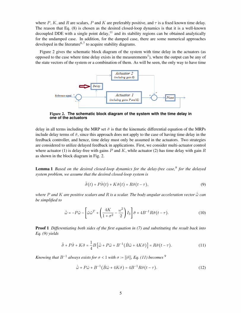
Figure 2 gives the schematic block diagram of the system with time delay in the actuators (asopposed to the case where time delay exists in the measurements1), where the output can be any ofthe state vectors of the system or a combination of them. As will be seen, the only way to have time

Figure 2. The schematic block diagram of the system with the time delay inone of the actuators

delay in all terms including the MRP set �� is that the kinematic differential equation of the MRPsinclude delay terms of ��, since this approach does not apply to the case of having time delay in thefeedback controller, and hence, time delay must only be assumed in the actuators. Two strategiesare considered to utilize delayed feedback in applications. First, we consider multi-actuator controlwhere actuator (1) is delay-free with gains P and K, while actuator (2) has time delay with gain Ras shown in the block diagram in Fig. 2.

Lemma 1 Based on the desired closed-loop dynamics for the delay-free case,9 for the delayedsystem problem, we assume that the desired closed-loop system is

¨��(t) + P ˙��(t) +K��(t) = R��(t − ⌧), (9)

where P and K are positive scalars and R is a scalar. The body angular acceleration vector ˙�! canbe simplified to

˙�! = −P �! − ��!�!T + � 4K

1 + �2− !2

2

� I3� �� + 4B−1R��(t − ⌧). (10)

Proof 1 Differentiating both sides of the first equation in (7) and substituting the result back intoEq. (9) yields

¨�� + P ˙�� +K�� = 1

4

B � ˙�! + P �! +B−1( ˙B�! + 4K��)� = R��(t − ⌧). (11)

Knowing that B−1 always exists for � < 1 with � ∶= ������, Eq. (11) becomes 9

˙�! + P �! +B−1( ˙B�! + 4K��) = 4B−1R��(t − ⌧). (12)

5

Taking the time derivative of matrix B in Eq. (6)

˙B = �− ˙��T �� − ��T˙��� I3 + ˙� + 2 ˙����T + 2�� ˙��T (13)

˙��T = 1

4

�!T �(1 − �2)I3 − 2� + 2����T � (14)

On the other hand,

�2 = ����T − �2I3 = ����T − ��T ��I3 (15)

Taking the time derivative of both sides of Eq. (15) we obtain

� ˙� + ˙�� = ˙����T + �� ˙��T − � ˙��T �� + ��T˙��� I3 = B, (16)

and calling

A ∶= � ˙�, AT ∶= ˙�� (17)

Eq. (16) can be written as

A +AT = B. (18)

Furthermore,

A −AT = ���0 �2�1 − �1�2 �1�3 − �1�3

�2�1 − �2�1 0 �2�3 − �3�2�3�1 − �3�1 �3�2 − �3�2 0

��� = ˙����T − �� ˙��T = C. (19)

Equations (16) and (19) can be solved for A and AT

� ˙� = A = 1

2

(B + C) = ˙����T − 1

2

� ˙��T �� + ��T˙��� I3,

˙�� = AT = �� ˙��T − 1

2

���T˙�� + ˙��T ��� I3, (20)

Also note that

BT = �1 + �2�2B−1 (21)

As is shown in Eq. (13), ˙B�! has a term ˙��! which is the hardest term to calculate. But, Eq. (14)implies that

�! = 4B−1 ˙�� = 4BT

(1 + �2)2 ˙��. (22)

Hence

˙��! = ˙�4BT

(1 + �2)2 ˙�� =4

(1 + �2)2 �(1 − �)2 ˙� ˙�� − 2 ˙�� ˙�� + 2 ˙�����T˙��� (23)

6

first term of which inside the brackets is zero. According to Eq. (15),

2

˙� �����T � ˙�� = 2 ˙� ��2 + ��T ��I3� ˙�� = 2 � ˙���� �� ˙��� + 2 ���T ��� � ˙� ˙��� = 2 � ˙��� �� ˙��� . (24)

Equation (23) can thus be written as

˙��! = 4

(1 + �2)2 �−2 ˙�� ˙�� + 2 ˙��� ˙��� = 8

˙��

(1 + �)2 (−I3 + �) ˙�� = −2

˙��

1 + �2(I3 + �) �!. (25)

However, substituting for ˙�� from Eq. (20) into Eq. (25) we obtain

˙��! = − 2

1 + �2��� ˙��T − 1

2

���T˙�� + ˙��T ��� I3� (I3 + �) �!

= 2

1 + �2�−�� ˙��T + ��T

˙��I3� (I3 + �) �!= 1

2 (1 + �2){(�2 − 1)!2�� + (1 + �2)(��T �!)�! − 2(�2!2)�� −(1 + �2)(��T �!)!��}, (26)

where ! ∶= ���!��.Other terms in Eq. (13) are easier to find

˙��T �� = ��T˙�� = 1

4

��TB�! = 1

4

(1 + �2)(��T �!), (27)

2

˙��(��T �!) = 1

2

�(1 − �T )I3 + 2� + 2����T � (��T �!)�!= 1

2

(1 − �2)(��T �!)�! − (��T �!)!�� + (��T �!)2��, (28)

and

2�� ˙��T �! = 1

2

���!T �(1 − �2)I3 − 2� + 2����T � �!= 1

2

(1 − �2)!2�� + ���!T !�� + (��T �!)2��. (29)

Substituting Eqs. (26), (27), (28), and (29) into Eq. (13) yields

˙B�! = −2(��T �!)!�� + 2(��T �!)2�� − 1

2

(1 + �2)!2�� + (1 − �2)(��T �!)�!. (30)

Substituting Eq. (30) into Eq. (12) yields

˙�! = −P �! − 1

(1 + �2)2 [−2(1 − �2)(��T �!)!�� + 2(1 − �2)(��T �!)2��−12

1 + �2(1 − �2)!2�� + (1 − �2)2(��T �!)�! + 4K(1 − �2)�� + 4(��T �!)�!��−2(1 − �2)(��T �!)��! + 4(��T �!)2�2�� − (1 + �2)!2�2�� + 2(1 − �2)(��T �!)2�� +8K�2��] + 4B−1R��(t − ⌧) (31)

7

The term 4(��T �!)�!�� in Eq. (31) is expressed as

− 4(��T �!)�2�! = −4(��T �!)(����T − ��T ��I3)�! = −4(��T �!)2�� + 4(��T �!)�2�!. (32)

Substituting Eq. (32) into Eq. (31) yields

˙�! = −P �! − 1

(1 + �2)2 [(��T �!)2��(2 − 2�2 + 2 − 2�2 − 4 + 4�2)+(��T �!)�!(1 − 2�2 + �4 + 4�2) + !2��(−1

2

+ �4

2

− �2 − �4) +K��(4 − 4�2 + 8�2)] + 4B−1R��(t − ⌧)

= −P �! − 1

(1 + �2)2 ��!(�!T ��)(1 + �2)2 − 1

2

(1 + �2)2!2�� + 4K(1 + �2)��� +4B−1R��(t − ⌧)

= −P �! − ��!�!T + � 4K

1 + �2− !2

2

� I3� �� + 4B−1R��(t − ⌧). (33)

The proof is, therefore, complete. �Equation (9) is written in the state-space form as

�x1 = ��, �x2 = ˙��, �x = � ��˙�� � (34)

˙�x = � ˙��¨�� � = � 03 I3−KI3 −PI3

�� ��(t)˙��(t) � + � 03 03

RI3 03�� ��(t − ⌧)

˙��(t − ⌧) � . (35)

Although, according to Eqs. (35) and (9), 6 DDEs are sufficient to acquire the dynamics behaviorof the closed-loop system, in order to include the plots for the time histories of the control signals(�u), as well, the system and the controller are modeled by 9 simultaneous DDEs in the MATLABdde23. Considering the second equation in (7) and Eq. (10) the following nonlinear relation for�u(t) is obtained

�u(t) = !(t)J �!(t) − JP �!(t) − J ��!(t)�!(t)T + � 4K

1 + �2(t) −!2(t)2

� I3� ��(t) +4J

1

(1 + �2(t))2BT (t)R��(t − ⌧), (36)

where Eq. (21) is used to obtain the expression for the controller.

It is instructive to compare our controller with the standard MRP-based control law9 using theLyapunov function

V (�!) = 1

2

�!TJ �! + 2K ln

�1 + ��T ��� . (37)

Taking the derivative along the trajectory and forcing it to be negative semidefinite as

˙V = �!T �J Bddt�! +K��� = −�!TP �! (38)

8

the corresponding asymptotic stabilizing control law9 for regulation control is obtained as

�u(t) = !(t)J �!(t) −P �!(t) −K��(t). (39)

However, the resulting closed-loop dynamics

JBddt�! +P �! +K�� = �0, (40)

where the superscript B indicates the time derivative with respect to the body frame, is not linear dueto the nonlinearities in Eq. (5). However, the inverse dynamics based control law given in Eq. (36)which has additional quadratic terms compared to the Lyapunov based control law in Eq. (39) doesin fact lead to a linear closed-loop dynamics.

In order to further analyze the closed-loop dynamics in Eq. (8), the time is nondimensionalizedas

t∗ = t

⌧,

d

dt= dt∗

dt

d

dt∗ =1

⌧

d

dt∗ ,d2

dt2= dt∗

dt

d

dt∗ �1

⌧

d

dt∗� =1

⌧2d2

dt∗2 (41)

Using the transformation Eq. (41) in Eq. (8), the latter becomes

��′′ + ⌧P ��′ + ⌧2K�� = ⌧2R��(t∗ − 1), (42)

which, considering the fact that P and K are scalars, can be written as three second order scalarDDEs

�′′i + ¯P�′i + ¯K�i = ¯R�i(t∗ − 1), i = 1,2,3 (43)

where prime and double prime “ ′ ”and “ ′′ ”represent for the first and second derivatives of thedimensionless parameter �i with respect to t∗, respectively, and ¯P = ⌧P , ¯K = ⌧2K, and ¯R = ⌧2R.Introducing the state-space variables in a similar manner as what we had in Eq. (34) for each i

z1 = �i, z2 = �′i. i = 1,2,3 (44)

Equation (42) can then be written in the state-space form

�z′ =A�z(t∗) +B�z(t∗ − 1), (45)

where

�z = � z1z2� , A = � 0 1− ¯K − ¯P � , B = ¯R� 0 0

1 0

� (46)

Two methods, an analytical approach and a numerical approach based on ChSCTA, are furtherimplemented to study the stability of the closed-loop system. The analytical approach only appliesto the time delay problem (45) for ¯P = 0 which can be referred to as the undamped case.

9

Analytical Investigation for the Undamped Case

Setting ¯P = 0 in Eq. (42), its corresponding characteristic equation can be written as

s2 + ¯K − ¯Re−s = 0. (47)

Since unstable systems have eigenvalues with positive real parts, s must be set equal to 0 and i! toobtain stability boundaries. If one sets s = 0 Eq. (47) yields the divergence stability boundary as

¯K = ¯R, (48)

while setting s = i! for ! ∈R, and separation of the real and imaginary parts yield

−!2 + ¯K − ¯R cos! = 0,¯R sin! = 0. (49)

Second equation in (49) yields

sin! = 0, or ¯R = 0. (50)

Solving Eqs. (50) and (49) simultaneously yields the flutter (Hopf) stability boundaries as

D =D1 ∪ D2, (51)

where

D1 = �( ¯K, ¯R)� ¯R = 0, ¯K > 0� ,D2 = �( ¯K, ¯R)� ¯K − ¯R(−1)n = n2⇡2� , n = 0,1,2,� (52)

This stability chart for the undamped case with straight lines, which is shown in Fig. 3 is knownas the Hsu-Bhatt-Vyshnegradskii stability chart in the literature.11

Corollary 1 The trivial solution of the DDE (43) is exponentially asymptotically stable if and onlyif there exists an integer n1 ≥ 0 such that either

¯R > 0, ¯R < ¯K − (2n1)2⇡2, and

¯R < − ¯K + (2n1 + 1)2⇡2 (53)

or

¯R < 0, ¯R > − ¯K + (2n1 + 1)2⇡2, and

¯R > ¯K − (2n1 + 2)2⇡2, (54)

Proof 2 Since the divergence boundary ¯K = ¯R is delay independent,12 for the system without thetime delay Eq. (49) becomes

s2 = ¯R − ¯K (55)

which results in the stable behavior for 0 ≤ ¯R < ¯K for the undamped system. Hence the regioninside the triangle △CDE is stable. On the other hand, by crossing through the divergence andHopf stability boundaries the number of unstable characteristic exponents (↵) increases by one andtwo, respectively (see Fig. 3). Since inside △CDE is stable with ↵ = 0, starting from a pointinside this triangle, if we cross through segment CD (which is the Hopf stability boundary) towardsoutside of that triangle, the parameter ↵ increases by 2, which means that we are in the unstableregion. Now if we move from a point on this unstable region towards inside△DFG by crossing thesegment DF , ↵ decreases by 2 again and becomes zero which implies that inside △DFG is alsostable. The same strategy can be followed for the other triangles. �

10

Figure 3. Hsu-Bhatt-Vyshnegradskii stability chart in ¯K − ¯R plane for ¯P = 0

obtained analytically.

The first set of conditions given in the Corollary 1 (Eq. 53) gives the stable triangles above the ¯Raxis, while the second set (Eq. 54) produces the stable triangles below that axis. Figure 3 representsthe stability chart obtained analytically in the ¯K − ¯R plane. The intersections of the first threeconsequent pairs of lines given in the set D2 in Eq. (52) are obtained analytically and representedin Fig. 3 along with the crossing points of the lines with the ¯K axis.

ChSCTA Method for the Damped Case

For the case ¯P ≠ 0, the characteristic equation is

s2 + ¯Ps + ¯K − ¯Re−s = 0, (56)

which, after setting s = j! and separating real and imaginary parts, yields

−!2 + ¯K − ¯R cos! = 0¯P! + ¯R sin! = 0. (57)

It can be seen that the flutter stability boundaries for this case do not remain as straight lines.However, like the undamped case, the ¯K = ¯R line can be seen to still correspond to the divergence(fold) instability. We now describe a numerical method used to investigate the stability of this case.

Chebyshev collocation points can be introduced as the projections of the equispaced points onthe upper half of the unit circle onto the horizontal axis, mathematically8

ti = cos i⇡N

. (58)

11

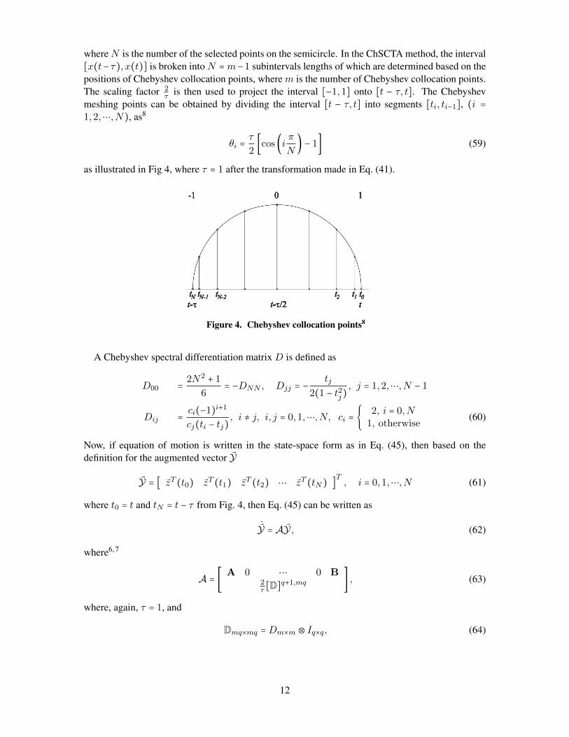
where N is the number of the selected points on the semicircle. In the ChSCTA method, the interval[x(t−⌧), x(t)] is broken into N =m−1 subintervals lengths of which are determined based on thepositions of Chebyshev collocation points, where m is the number of Chebyshev collocation points.The scaling factor 2

⌧ is then used to project the interval [−1,1] onto [t − ⌧, t]. The Chebyshevmeshing points can be obtained by dividing the interval [t − ⌧, t] into segments [ti, ti−1], (i =1,2,�,N), as8

✓i = ⌧

2

�cos�i ⇡N� − 1� (59)

as illustrated in Fig 4, where ⌧ = 1 after the transformation made in Eq. (41).

Figure 4. Chebyshev collocation points8

A Chebyshev spectral differentiation matrix D is defined as

D00 = 2N2 + 16

= −DNN , Djj = − tj

2(1 − t2j) , j = 1,2,�,N − 1Dij = ci(−1)i+1

cj(ti − tj) , i ≠ j, i, j = 0,1,�,N, ci = � 2, i = 0,N1, otherwise

(60)

Now, if equation of motion is written in the state-space form as in Eq. (45), then based on thedefinition for the augmented vector �Y

�Y = � �zT (t0) �zT (t1) �zT (t2) � �zT (tN) �T , i = 0,1,�,N (61)

where t0 = t and tN = t − ⌧ from Fig. 4, then Eq. (45) can be written as

˙�Y = A �Y , (62)

where6, 7

A = � A 0 � 0 B2⌧ [D]q+1,mq � , (63)

where, again, ⌧ = 1, and

Dmq×mq =Dm×m ⊗ Iq×q, (64)

12

Figure 5. Stability chart in ¯K − ¯R plane (Right) for ¯P = 0,1,2,3,4 obtainedanalytically for ¯P = 0 and numerically using ChSCTA for ¯P > 0. The ∗ and● shown represent the points simulated in Figs. 11 and 12, while ▲ and �represent the points simulated in Figs. 9 and 10, respectively.

and only rows of D between q + 1 and mq are taken into account. Based on the left half-planeanalysis, the real parts of the eigenvalues of the matrix A in Eq. (63) determine the stability of thesystem such that if all eigenvalues of matrixA have negative real parts then system is asymptoticallystable.

ChSCTA is applied to produce the Figs. 5, 6, and 7 using 85 Chebyshev collocation points inthe 50 × 50 meshgrid. The second strategy is delay stabilization of an otherwise unstable system.The small region magnified in Fig. 5 illustrates how the added delay term stabilizes an otherwiseunstable system when K < 0. The behavior of the system in the ¯K − ¯R plane is plotted in Fig. 5for different values of ¯P which can be referred to as the damping of the system (43). As mentionedbefore, the stability boundaries do not remain as straight lines for the damped cases except for the¯R = ¯K divergence boundary which remains straight. Figure 6 shows the stable region in the ⌧ −Rdiagram for P =K = 4 (Left), and for P = 3 and K = 1 (Right). Referring to this figure, the systemis unstable for R > 1 when P = 3 and K = 1. In order to find the proper values of ¯P and ¯K whichstabilize the system for some ¯R > 1 (which corresponds to R > 1 for ⌧ = 1), the stability is studiedin the ¯K − ¯P space in Fig. 7, with ¯R = 2 (Left) and R = 6.5 (Right), using 85 Chebyshev collocationpoints in a 50 × 50 meshgrid. As can be inferred from these plots, for ¯P = ¯K = 4 the MRPs of thesystem are in the stable region when ¯R = 2.

It should be noted that if system is just barely stable, then a small error or uncertainty in thesystem parameters could push the system over the stability boundary. Hence, it is often desiredto design systems with some margin of error. The relative stability is compared with the stabilityboundary for ¯P = 1, for instance, in the ¯K − ¯R plane as shown in Fig. 8. For the relative stabilityboundary in the figure, the spectral abscissae are assumed to be equal to −0.01, −0.05, −0.07, −0.1.

SIMULATION RESULTS

In this section, in order to verify the stability charts, and to study the effect of the proposedcontroller on the system, using MATLAB dde23, the time histories for arbitrarily picked stableand unstable points are produced for the time delayed system. Time histories of the system are

13

Figure 6. ⌧ −R plot for the closed-loop equation of the controlled system (42),S stable, U unstable; P = K = 4 (Left); P = 3, K = 1 (Right) obtained numer-ically using ChSCTA. The ∗ and ● shown represent the points simulated inFig. 11.

further obtained for the delay-free system to compare with the literature.

In order to depict delay stabilization caused by the intentional time delay added to the system,for a negative value K = −2, simulations are performed for the non-delayed system as well as thedelayed system with R = −4 and ⌧ = 1 sec. The corresponding results shown in Figs. 9 and 10 agreewith the stability chart given in Fig. 5.

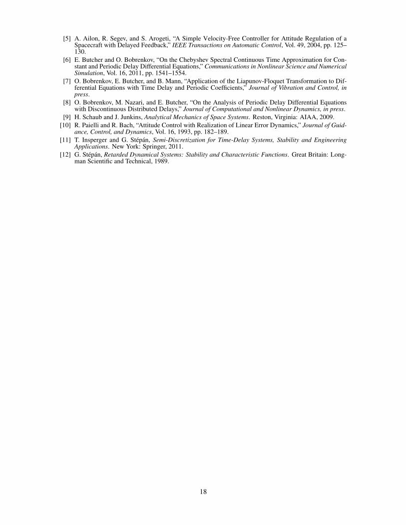
Two points, one from the stable region shown with ∗ and the other one from the unstable regionshown with ●, are arbitrarily picked for which time series are plotted in Figs. 11 and 12. These timehistories are consistent with the regions of stability and instability shown in Figs. 5, 6, and 7 fordifferent pairs of parameter planes. The state-space form of Eq. (8) without transformation does notdiffer significantly from Eq. (35). Since the angular velocity response is also studied, the state-spacevector �y contains the angular velocity vector �!

˙�y = ���03 I3 03−KI3 −PI3 03

03 03 −PI3

��� �y(t) +���

03 03 03

RI3 03 03

03 03 03

��� �y(t − ⌧) + �f(�y) (65)

where �y = � ��T˙��T �!T �T , as mentioned before, and the nonlinear terms are

�f(�y) =�����������

03

03−f ��!�!T + � 4K1+�2 − !2

2 � I3� �� + 4B−1R��(t − ⌧)�����������. (66)

First, for the same values as in the delay-free case, and the stability chart for the Eq. (8) is to beprovided in the R − ⌧ plane. The time series shown in Fig. 11 approve the stability of the angularvelocity and the MRPs of the closed-loop controlled delayed system with the initial parameter valuesgiven in Table 1 using the aforementioned control law (36) for R = 2 and ⌧ = 0.5 sec. However,according to Fig. 6, the satellite attitude is expected to be unstable for R > 4, and the predictableunstable behavior is shown in Fig. 12 for the same time delay as that in Fig. 11.

14

Figure 7. ¯K− ¯P plot for the closed-loop equation of the controlled system (42),S stable, U unstable, ¯R = 2 (Left); ¯R = 6.5 (Right) obtained numerically usingChSCTA. The ∗ and ● shown represent the points simulated in Fig. 11.

Figure 8. Relative (black) and absolute (gray) stability charts in ¯K − ¯R plane(Right) for ¯P = 1. The spectral abscissae for the relative stability bound-aries are −0.01 (solid line), −0.05 (dashed dotted line), −0.07 (dotted line), −0.1(dashed line).

15

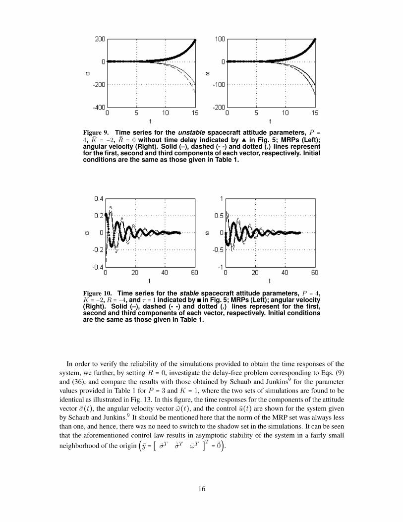
Figure 9. Time series for the unstable spacecraft attitude parameters, ¯P =4, ¯K = −2, ¯R = 0 without time delay indicated by ▲ in Fig. 5; MRPs (Left);angular velocity (Right). Solid (–), dashed (- -) and dotted (.) lines representfor the first, second and third components of each vector, respectively. Initialconditions are the same as those given in Table 1.

Figure 10. Time series for the stable spacecraft attitude parameters, P = 4,K = −2, R = −4, and ⌧ = 1 indicated by � in Fig. 5; MRPs (Left); angular velocity(Right). Solid (–), dashed (- -) and dotted (.) lines represent for the first,second and third components of each vector, respectively. Initial conditionsare the same as those given in Table 1.

In order to verify the reliability of the simulations provided to obtain the time responses of thesystem, we further, by setting R = 0, investigate the delay-free problem corresponding to Eqs. (9)and (36), and compare the results with those obtained by Schaub and Junkins9 for the parametervalues provided in Table 1 for P = 3 and K = 1, where the two sets of simulations are found to beidentical as illustrated in Fig. 13. In this figure, the time responses for the components of the attitudevector ��(t), the angular velocity vector �!(t), and the control �u(t) are shown for the system givenby Schaub and Junkins.9 It should be mentioned here that the norm of the MRP set was always lessthan one, and hence, there was no need to switch to the shadow set in the simulations. It can be seenthat the aforementioned control law results in asymptotic stability of the system in a fairly smallneighborhood of the origin ��y = � ��T

˙��T �!T �T = �0�.

16

Table 1. Parameter values9

Parameter Value

J diag[ 30 20 10 ] kg.m2

��(t0) � −.3 −.4 .2 �T�!(t0) � .2 .2 .2 �T

CONCLUSIONS AND FUTURE WORK

In this paper, a nonlinear delayed control law has been introduced to acquire the desired closed-loop dynamics of a typical rigid spacecraft. As opposed to authors’ other work1 where the timedelay is considered in the measurements, the time delay here has been assumed to be in the ac-tuators. Two strategies are considered. In the first strategy, one actuator is delay-free, while theother one has time delay. Delay stabilization is another strategy, where intentional time delay isintroduced into the actuator in order to stabilize the closed-loop dynamics which would be unstablewithout delay. The stability boundaries are obtained analytically for the undamped delayed closed-loop system which is known as the Hsu-Bhatt-Vyshnegradskii stability chart, where the stabilityregions appear as triangles in which the number of unstable characteristic exponents is zero. Sta-bility boundaries, however, do not remain as straight lines, for the damped system, nor can they beinvestigated analytically, and hence ChSCTA has been implemented instead to obtain the stabilityboundaries for the damped case. MATLAB dde23 has been applied further to obtain the timehistories of the system which have been in agreement with the stability charts. Finally, in order toverify the controller, the time series obtained for the controlled delay-free system are compared tothose in the literature.

This work hopes to be a first step toward further understanding the following important issues.First, the control gains P and K are selected arbitrary in this study. In control design, it is usuallyimportant, however, to design the gains of the closed-loop dynamics for specified performance suchas critical damping. Second, unmodeled external torques due to effects such as atmospheric drag orbearing friction can cause steady state errors which should be eliminated or diminished by addingan integral feedback term. We are also looking into ways to extend the method introduced in thepresent work to do the attitude tracking problem.

ACKNOWLEDGMENTS

Financial support from the National Science Foundation under Grant Nos. CMMI-0900289 andCMMI-1131646 is gratefully acknowledged.

REFERENCES[1] E. Samiei, M. Nazari, E. Butcher, and H. Schaub, “Delayed Feedback Control of Rigid Body Atti-

tude using Neural Networks and Lyapunov-Krasovskii Functionals,” AAS/AIAA Spaceflight MechanicsMeeting, Charleston, SC, Paper No. 12-168, Jan. 29–Feb. 2, 2012.

[2] C. Hall, P. Tsiotras, and H. Shen, “Tracking Rigid Body Motion Using Thrusters and MomentumWheels,” Journal of the Astronautical Sciences, Vol. 50, 2002, pp. 311–323.

[3] P. Tsiotras, H. Shen, and C. Hall, “Satellite Attitude Control and Power Tracking with En-ergy/Momentum Wheels,” Journal of Guidance, Control, and Dynamics, Vol. 24, 2001, pp. 23–34.

[4] A. Chunodkar and M. Akella, “Attitude Stabilization with Unknown Bounded Delay in Feedback Con-trol Implementation,” Journal of Guidance, Control, and Dynamics, Vol. 34, 2011, pp. 533–542.

17

[5] A. Ailon, R. Segev, and S. Arogeti, “A Simple Velocity-Free Controller for Attitude Regulation of aSpacecraft with Delayed Feedback,” IEEE Transactions on Automatic Control, Vol. 49, 2004, pp. 125–130.

[6] E. Butcher and O. Bobrenkov, “On the Chebyshev Spectral Continuous Time Approximation for Con-stant and Periodic Delay Differential Equations,” Communications in Nonlinear Science and NumericalSimulation, Vol. 16, 2011, pp. 1541–1554.

[7] O. Bobrenkov, E. Butcher, and B. Mann, “Application of the Liapunov-Floquet Transformation to Dif-ferential Equations with Time Delay and Periodic Coefficients,” Journal of Vibration and Control, inpress.

[8] O. Bobrenkov, M. Nazari, and E. Butcher, “On the Analysis of Periodic Delay Differential Equationswith Discontinuous Distributed Delays,” Journal of Computational and Nonlinear Dynamics, in press.

[9] H. Schaub and J. Junkins, Analytical Mechanics of Space Systems. Reston, Virginia: AIAA, 2009.[10] R. Paielli and R. Bach, “Attitude Control with Realization of Linear Error Dynamics,” Journal of Guid-

ance, Control, and Dynamics, Vol. 16, 1993, pp. 182–189.[11] T. Insperger and G. Stepan, Semi-Discretization for Time-Delay Systems, Stability and Engineering

Applications. New York: Springer, 2011.[12] G. Stepan, Retarded Dynamical Systems: Stability and Characteristic Functions. Great Britain: Long-

man Scientific and Technical, 1989.

18

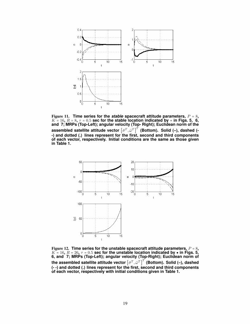
Figure 11. Time series for the stable spacecraft attitude parameters, P = 8,K = 16, R = 8, ⌧ = 0.5 sec for the stable location indicated by ∗ in Figs. 5, 6,and 7; MRPs (Top-Left); angular velocity (Top- Right); Euclidean norm of theassembled satellite attitude vector ���T , �!T �T (Bottom). Solid (–), dashed (--) and dotted (.) lines represent for the first, second and third componentsof each vector, respectively. Initial conditions are the same as those givenin Table 1.

Figure 12. Time series for the unstable spacecraft attitude parameters, P = 8,K = 16, R = 26, ⌧ = 0.5 sec for the unstable location indicated by ● in Figs. 5,6, and 7; MRPs (Top-Left); angular velocity (Top-Right); Euclidean norm ofthe assembled satellite attitude vector ���T , �!T �T (Bottom). Solid (–), dashed(- -) and dotted (.) lines represent for the first, second and third componentsof each vector, respectively with initial conditions given in Table 1.

19

Figure 13. Time history of �� (first row, left), �u (first row, right), and �! (thirdrow) with dotted lines (.) representing the norms, and solid lines (–), dasheddotted lines (-.), and dashed lines (- -) representing the first, second and thirdcomponents of each vector, respectively, as compared to �� (second row, left)and �u (second row, right) given by Schaub and Junkins9 .

20