Magnetically levitated planar actuator with moving ... - CiteSeerX
125
Magnetically levitated planar actuator with moving magnets: Dynamics, commutation and control design PROEFSCHRIFT ter verkrijging van de graad van doctor aan de Technische Universiteit Eindhoven, op gezag van de Rector Magnificus, prof.dr.ir. C.J. van Duijn, voor een commissie aangewezen door het College voor Promoties in het openbaar te verdedigen op dinsdag 15 januari 2008 om 16.00 uur door Cornelis Martinus Maria van Lierop geboren te Eindhoven
-
Upload
khangminh22 -
Category
Documents
-
view
0 -
download
0
Transcript of Magnetically levitated planar actuator with moving ... - CiteSeerX

Magnetically levitated planar actuator with moving
magnets: Dynamics, commutation and control design
PROEFSCHRIFT
ter verkrijging van de graad van doctor aan deTechnische Universiteit Eindhoven, op gezag van de
Rector Magnificus, prof.dr.ir. C.J. van Duijn, voor eencommissie aangewezen door het College voor
Promoties in het openbaar te verdedigenop dinsdag 15 januari 2008 om 16.00 uur
door
Cornelis Martinus Maria van Lierop
geboren te Eindhoven

Dit proefschrift is goedgekeurd door de promotoren:
prof.dr.ir. P.P.J. van den Bosch
en
prof.dr.ir. A.J.A. Vandenput
Copromotor:
dr.ir. A.A.H. Damen
This work is part of the IOP-EMVT program (Innovatiegerichteonderzoeksprogramma’s - Elektromagnetische vermogenstech-niek). This program is funded by SenterNovem, an agency ofthe Dutch Ministry of Economic Affairs.
This dissertation has been completed in fulfillment of the re-quirements of the Dutch Institute of Systems and Control DISC.
Copyright c©2008 by C.M.M. van Lierop
Coverdesign by AtelJ van Lierop Bladel and Studio Interpoint Netersel
CIP-DATA LIBRARY TECHNISCHE UNIVERSITEIT EINDHOVEN
Lierop, Cornelis M.M. van
Magnetically levitated planar actuator with moving magnets : dynamics,commutation and control design / by Cornelis Martinus Maria van Lierop. -Eindhoven : Technische Universiteit Eindhoven, 2008.Proefschrift. - ISBN 978-90-386-1704-6NUR 959Trefw.: magnetische levitatie / elektrische machines ; regelingen / lineaireelektromotoren / elektrische aandrijvingen ; regelen.Subject headings: commutation / magnetic levitation / machine control / linearmotors.

Aan Chantal, Els, John en Willem

iv
Abstract
Magnetically levitated planar actuator with moving
magnets: Dynamics, commutation and control design
Mechanical systems with multiple degrees of freedom typically consist of severalone degree-of-freedom electromechanical actuators. Most of these electromechani-cal actuators have a standard, often integrated, commutation (i.e. linearization anddecoupling) algorithm deriving the actuator inputs which result in convenient con-trol properties and relatively simple actuator constraints. Instead of using severalone degree-of-freedom actuators, it is sometimes advantageous to combine multipledegrees of freedom in one actuator to meet the ever more demanding performancespecifications. Due to the integration of the degrees of freedom, the resulting com-mutation and control algorithms are more complex. Therefore, the involvement ofcontrol engineering during an early stage of the design phase of this class of actu-ators is of paramount importance. One of the main contributions of this thesis isa novel commutation algorithm for multiple degree-of-freedom actuators and theanalysis of its design implications.
A magnetically levitated planar actuator is an example of a multiple degree offreedom electromechanical actuator. This is an alternative to xy-drives, which areconstructed of stacked linear motors, in high-precision industrial applications. Thetranslator of these planar actuators is suspended above the stator with no supportother than magnetic fields. Because of the active magnetic bearing the translatorneeds to be controlled in all six mechanical degrees of freedom. This thesis presentsthe dynamics, commutation and control design of a contactless, magnetically lev-itated, planar actuator with moving magnets. The planar actuator consists of astationary coil array, above which a translator consisting of an array of permanentmagnets is levitated. The main advantage of this actuator is that no cables from
v
vi Abstract
the stator to the translator are required. Only coils below the surface of the magnetarray effectively contribute to its levitation and propulsion. Therefore, the set ofactive coils is switched depending on the position of the translator in the xy-plane.The switching in combination with the contactless translator, in principle, allowsfor infinite stroke in the xy-plane.
A model-based commutation and control approach is used throughout thisthesis using a real-time analytical model of the ironless planar actuator. The real-time model is based on the analytical solutions to the Lorentz force and torqueintegrals. Due to the integration of propulsion in the xy-plane with an active mag-netic bearing, standard decoupling schemes for synchronous machines cannot beapplied to the planar actuator to linearize and decouple the force and the torquecomponents. Therefore, a novel commutation algorithm has been derived whichinverts the fully analytical mapping of the force and torque exerted by the set ofactive coils as a function of the coil currents and the position and orientation of thetranslator. Additionally, the developed commutation algorithm presents an optimalsolution in the sense that it guarantees minimal dissipation of energy. Another im-portant contribution of this thesis is the introduction of smooth position dependentweighing functions in the commutation algorithm. These functions enable smoothswitching between different active coil sets, enabling, in principle, an unlimitedstroke in the xy-plane. The resulting current waveform through each individuallyexcited active coil is non-sinusoidal.
The model-based approach, in combination with the novel commutation al-gorithm, resulted in a method to evaluate/design controllable topologies. Usingthis method several stator coil topologies are discussed in this thesis. Due to thechanging amount of active coils when switching between active coil sets, the actu-ator constraints (i.e. performance) depend on the xy-position of the translator. Ananalysis of the achievable acceleration as a function of the position of the translatorand the current amplifier constraints is given. Moreover, the dynamical behavior ofthe decoupled system is analyzed for small errors and a stabilizing control structurehas been derived.
One of the derived coil topologies called the Herringbone Pattern Planar Ac-tuator (HPPA) has been analyzed into more detail and it has been manufactured.The stator of the actuator consists of a total of 84 coils, of which between 15 and24 coils are simultaneously used for the propulsion and levitation of the translator.The real-time model, the dynamic behavior and the commutation algorithm havebeen experimentally verified using this fully-operational actuator. The 6-DOF con-tactless, magnetically levitated, planar actuator with moving magnets (HPPA) hasbeen designed and tested and is now operating successfully according to all initialdesign and performance specifications.
Contents
1 Introduction 1
1.1 Background . . . . . . . . . . . . . . . . . . . . . . . . . . . . . 2
1.2 Research objectives . . . . . . . . . . . . . . . . . . . . . . . . . 4
1.3 Organization of the thesis . . . . . . . . . . . . . . . . . . . . . . 5
2 Commutation of basic forcer topologies using dq0 transformation 7
2.1 Introduction . . . . . . . . . . . . . . . . . . . . . . . . . . . . . 7
2.2 Rotating machines . . . . . . . . . . . . . . . . . . . . . . . . . . 8
2.3 Linear actuators . . . . . . . . . . . . . . . . . . . . . . . . . . . 12
2.4 Basic forcer topologies for planar motion . . . . . . . . . . . . . 16
3 Linearization and decoupling of the wrench 21
3.1 Introduction . . . . . . . . . . . . . . . . . . . . . . . . . . . . . 21
3.2 Real-time analytical six degree-of-freedom coil model . . . . . . 22
3.3 Direct wrench-current decoupling . . . . . . . . . . . . . . . . . 29
3.3.1 Switching . . . . . . . . . . . . . . . . . . . . . . . . 32
3.4 Force and torque decomposition . . . . . . . . . . . . . . . . . . 45
4 Design of controllable topologies 49
4.1 Introduction . . . . . . . . . . . . . . . . . . . . . . . . . . . . . 49
4.2 State controllability conditions of a planar actuator . . . . . . . 49
4.3 Error sensitivity of weighted minimal norm inverses and solutions 53
4.4 Controllable 6 DOF basic topologies . . . . . . . . . . . . . . . . 55
4.5 Worst-case force components . . . . . . . . . . . . . . . . . . . . 62
5 Experiments 67
5.1 Introduction . . . . . . . . . . . . . . . . . . . . . . . . . . . . . 67
vii
viii Contents
5.2 Experimental setup . . . . . . . . . . . . . . . . . . . . . . . . . 675.2.1 HPPA prototype . . . . . . . . . . . . . . . . . . . . 675.2.2 Test bench . . . . . . . . . . . . . . . . . . . . . . . 68
5.3 Control structure . . . . . . . . . . . . . . . . . . . . . . . . . . 765.4 Measurement results . . . . . . . . . . . . . . . . . . . . . . . . 82
5.4.1 Closed-loop identification . . . . . . . . . . . . . . . 825.4.2 Tracking performance . . . . . . . . . . . . . . . . . 89
6 Conclusions and recommendations 956.1 Model based commutation algorithm . . . . . . . . . . . . . . . 956.2 Linking control to the design proces . . . . . . . . . . . . . . . . 966.3 Realization and test of the prototype . . . . . . . . . . . . . . . . 966.4 Outlook towards future developments . . . . . . . . . . . . . . . 97
6.4.1 Full rotation about the z-axis . . . . . . . . . . . . . 976.4.2 Planar actuators with non-holonomic constraints . . 976.4.3 Fault tolerant planar actuator commutation . . . . . 976.4.4 Wireless power transfer, data communication and
control . . . . . . . . . . . . . . . . . . . . . . . . . 976.4.5 Multiple translators above one stator . . . . . . . . . 98
A Schur complement 99
B Proof of theorem 4.7 101
C List of symbols 103
Bibliography 105
Samenvatting - Dutch abstract 111
Dankwoord - Acknowledgements 115
Curriculum Vitae 117

Chapter 1
Introduction
The field of control engineering is often only involved at the final stage of a project.This can sometimes lead to problems when the design is not optimal with respectto the control objectives which are necessary for obtaining the desired functionality.The design of electromechanical machines is no exception to this observation sincethey are often designed first and the control issues are dealt with later. To be able tocontrol the machine, often a non-linear decoupling called the dq0- or Park’s transfor-mation [33, 34] is applied to linearize the machine properties which are necessaryfor control. This commutation method works fine for most electrical machines be-cause the non-linear mapping has very convenient properties like orthonormalityand power invariance. Moreover, most electromechanical machines only actuatea single degree-of-freedom. However, when more mechanical degrees-of-freedom(DOF) are combined in the electromechanical design of the actuator, the sequentialapproach described above is not valid anymore. Due to the multiple degrees-of-freedom, concepts like directionality, linearization by feedback, controllability, andthe resulting complex actuator constraints start to play a major role in the designprocess. Moreover, in some cases even the traditional dq0-transformation cannot beapplied effectively. Consequently, the traditional assumptions about control whichare made during the design phase of the machine do not hold anymore, resultingin the need for a larger involvement of control engineering aspects during the de-sign process. This thesis focusses on the design aspects of planar actuators withintegrated magnetic bearing related to the controllability. Nevertheless, the theoryderived is not limited to this class of actuators. The planar actuators discussed inthis thesis consist of a translator with permanent magnets which is levitated above
1
2 Chapter 1. Introduction
an array of coils. The translator has an, in principle, unlimited stroke in the hori-zontal plane.
The main focus is on how to obtain a suitable commutation algorithm whichboth exploits the possibilities of the actuator as well as obtaining an implementablecontrol solution. In order to achieve better understanding of the mechanisms in-volved in creating a planar actuator and its controller, a model based approach isused.
1.1 Background
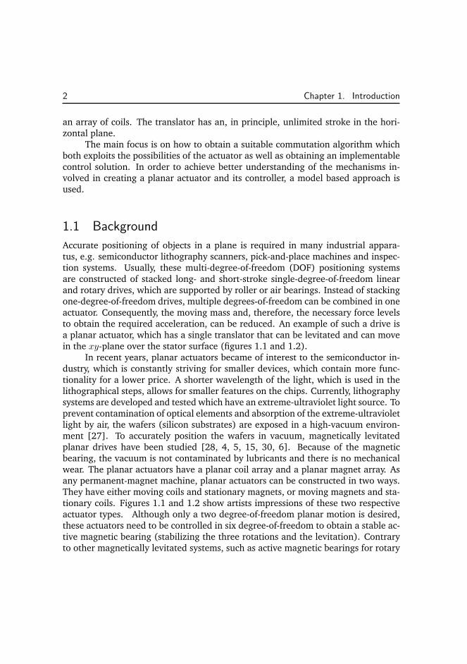
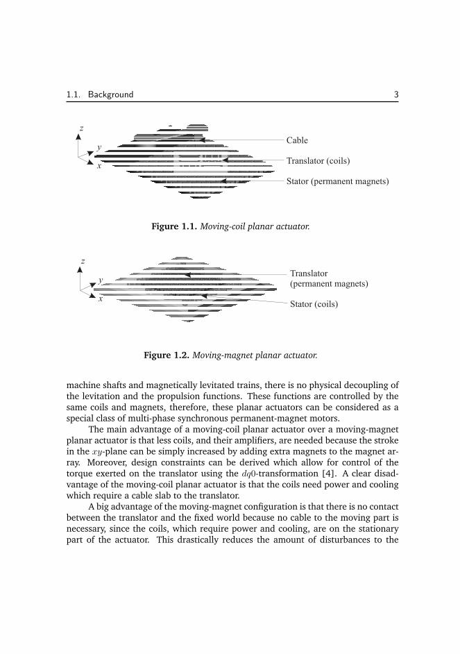
Accurate positioning of objects in a plane is required in many industrial appara-tus, e.g. semiconductor lithography scanners, pick-and-place machines and inspec-tion systems. Usually, these multi-degree-of-freedom (DOF) positioning systemsare constructed of stacked long- and short-stroke single-degree-of-freedom linearand rotary drives, which are supported by roller or air bearings. Instead of stackingone-degree-of-freedom drives, multiple degrees-of-freedom can be combined in oneactuator. Consequently, the moving mass and, therefore, the necessary force levelsto obtain the required acceleration, can be reduced. An example of such a drive isa planar actuator, which has a single translator that can be levitated and can movein the xy-plane over the stator surface (figures 1.1 and 1.2).
In recent years, planar actuators became of interest to the semiconductor in-dustry, which is constantly striving for smaller devices, which contain more func-tionality for a lower price. A shorter wavelength of the light, which is used in thelithographical steps, allows for smaller features on the chips. Currently, lithographysystems are developed and tested which have an extreme-ultraviolet light source. Toprevent contamination of optical elements and absorption of the extreme-ultravioletlight by air, the wafers (silicon substrates) are exposed in a high-vacuum environ-ment [27]. To accurately position the wafers in vacuum, magnetically levitatedplanar drives have been studied [28, 4, 5, 15, 30, 6]. Because of the magneticbearing, the vacuum is not contaminated by lubricants and there is no mechanicalwear. The planar actuators have a planar coil array and a planar magnet array. Asany permanent-magnet machine, planar actuators can be constructed in two ways.They have either moving coils and stationary magnets, or moving magnets and sta-tionary coils. Figures 1.1 and 1.2 show artists impressions of these two respectiveactuator types. Although only a two degree-of-freedom planar motion is desired,these actuators need to be controlled in six degree-of-freedom to obtain a stable ac-tive magnetic bearing (stabilizing the three rotations and the levitation). Contraryto other magnetically levitated systems, such as active magnetic bearings for rotary
1.1. Background 3
Figure 1.1. Moving-coil planar actuator.
Figure 1.2. Moving-magnet planar actuator.
machine shafts and magnetically levitated trains, there is no physical decoupling ofthe levitation and the propulsion functions. These functions are controlled by thesame coils and magnets, therefore, these planar actuators can be considered as aspecial class of multi-phase synchronous permanent-magnet motors.
The main advantage of a moving-coil planar actuator over a moving-magnetplanar actuator is that less coils, and their amplifiers, are needed because the strokein the xy-plane can be simply increased by adding extra magnets to the magnet ar-ray. Moreover, design constraints can be derived which allow for control of thetorque exerted on the translator using the dq0-transformation [4]. A clear disad-vantage of the moving-coil planar actuator is that the coils need power and coolingwhich require a cable slab to the translator.
A big advantage of the moving-magnet configuration is that there is no contactbetween the translator and the fixed world because no cable to the moving part isnecessary, since the coils, which require power and cooling, are on the stationarypart of the actuator. This drastically reduces the amount of disturbances to the
4 Chapter 1. Introduction
translator. A disadvantage of the moving-magnet planar actuator, however, is theincreased complexity of the torque decoupling as a function of position. Variousproposals to control the moving-magnet torque using the dq0-decomposition havebeen made in patent literature [41, 40, 1, 2]. However, the resulting disturbancetorque remains significant. Moreover, in a moving-magnet planar actuator, only thecoils below and near the edges of the magnet array can exert force and torque onthe magnet array. Therefore, when long-stroke motion in the xy-plane is desired,the set of active coils has to be switched. No literature on the design and controlaspects of switching the set of active coils, without influencing the force and torquedecoupling, has been found.
1.2 Research objectives
Using traditional synchronous electrical machine theory to design/control long-stroke moving-magnet planar actuators with integrated magnetic bearing does notlead to practical results (see section 1.1). However, this class of actuators has theadvantage of contactless levitation and propulsion, resulting in small translator dis-turbances. Therefore, the need for new electromechanical design and control the-ories arises to study and design this class of actuators. Consequently, research intoobtaining both an efficient as well as a real-time controllable electromechanicaldesign calls for the combination of the electromechanical design and control dis-ciplines. The research into the control and electromechanical design aspects has,therefore, been carried out in parallel by two PhD students and the results are de-scribed in two theses. This thesis focusses on the commutation, the controllabilityof planar actuator designs and the control of the realized planar actuator, whereasthe thesis of Jansen [17] focusses on the modeling and design of the planar actua-tor. To validate the derived theory, and to assure that all critical design aspects arecovered, a proof-of-principle device has been created. The general project objec-tives discussed in this thesis, therefore, can be summarized by the following threesub-objectives:
• Research of model-based commutation algorithms which linearize and de-couple the system. Due to the nature of long-stroke moving-magnet planaractuators the classical machine theory which is used to derive a suitablecommutation algorithm cannot be applied effectively. The main reasonscreating this problem are the larger influence of the ”disturbance” torquewhen using sinusoidal currents and the need to switch active coil sets whenlong-stroke movement is applied. (chapters 2 and 3)
• Research the link between the commutation algorithm and the design pro-
1.3. Organization of the thesis 5
cess. Since the commutation algorithms need to be both fast and accurate,the complexity of the (real-time) model and the commutation algorithmneeds to be low but still sufficiently accurate to represent the system be-havior. Moreover, the desired motion-profiles, the influence of the loca-tion of the mass-center-point and the noise-distribution over the degrees-of-freedom also play an important role in both the electromechanical aswell as the control design. (chapters 3 and 4)
• Research the effectiveness of the derived theory by using a proof-of-principledevice. Because of the large amount of parameters in combination with thenon-linear behavior of the system, a proof-of-principle device is realized tovalidate the models and the decoupling algorithm. (chapter 5)
1.3 Organization of the thesis
Although the work presented in this thesis heavily depends on the theory derived in[17] it can be read independently. Consequently, there are some overlapping parts.
Chapter 2 focusses on the dq0- or Park’s transformation which is traditionallyused to decouple and control synchronous actuators. The transformation is adaptedto create basic planar forcer topologies (a stator-coil layout which can be used toproduce position independent forces). These forcer topologies are the buildingblocks of the examples which are used throughout this thesis. A new direct wrench-current decoupling algorithm is derived in chapter 3 (where the wrench is definedas a vector which consists of both force and torque components). Using this newalgorithm it is possible to decouple the force and torque components of ironlessmoving-magnet planar actuators with integrated magnetic bearing. Only coils be-low the magnet array effectively contribute to the levitation and propulsion of thetranslator. Therefore, the decoupling algorithm is adapted to include switching be-tween active coil sets enabling the design and control of long-stroke actuators. Fur-thermore, conditions are derived which have to be met for decoupling to function.At the end of this chapter it is shown that, in the case of ironless planar actuators,the dq0 transformation can be seen as a subclass of the new commutation strategy.Chapter 4 focusses on how to design controllable topologies, using the derived com-mutation algorithm of chapter 3. The theory discussed throughout both this thesisas well as the thesis of Jansen [17] has been used to create a fully functioning pro-totype called the Herringbone Pattern Planar Actuator (HPPA). Measurements onthe controlled HPPA are presented in chapter 5. Conclusions and recommendationsfor future work are given in chapter 6.

6 Chapter 1. Introduction
Chapter 2
Commutation of basic forcer
topologies using dq0
transformation
2.1 Introduction
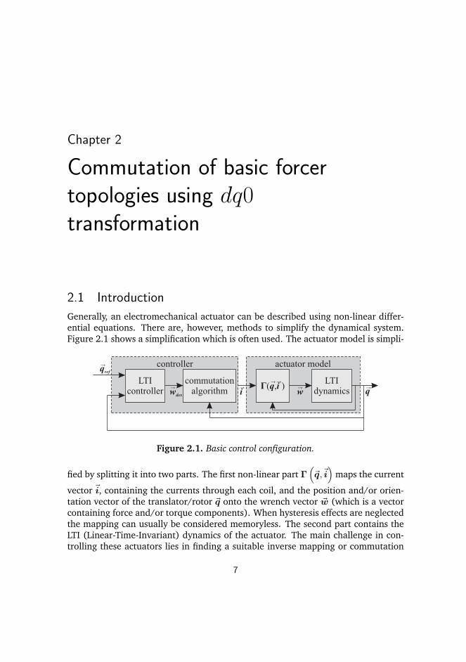
Generally, an electromechanical actuator can be described using non-linear differ-ential equations. There are, however, methods to simplify the dynamical system.Figure 2.1 shows a simplification which is often used. The actuator model is simpli-
Figure 2.1. Basic control configuration.
fied by splitting it into two parts. The first non-linear part Γ
(
~q,~i)
maps the current
vector ~i, containing the currents through each coil, and the position and/or orien-tation vector of the translator/rotor ~q onto the wrench vector ~w (which is a vectorcontaining force and/or torque components). When hysteresis effects are neglectedthe mapping can usually be considered memoryless. The second part contains theLTI (Linear-Time-Invariant) dynamics of the actuator. The main challenge in con-trolling these actuators lies in finding a suitable inverse mapping or commutation
7
8 Chapter 2. Commutation of basic forcer topologies using dq0 transformation
algorithm which linearizes and decouples the system by feedback. Classically, formost rotating (and linear) actuators this inverse mapping is achieved using the dq0or Park’s transformation which will be discussed in more detail in sections 2.2 and2.3. Section 2.4 shows how (parts of) the dq0 transformation can be expandedtowards planar actuators. Moreover, section 2.4 also shows some basic coil config-urations which can be used as building blocks for planar actuators.
2.2 Rotating machines
Classically the dq0 transformation was derived for rotating machines. However,the theory is not restricted to this class of machines. In order to understand theadapted versions of the dq0 transformation this section summarizes the classicaltheory applied to permanent-magnet synchronous machines.
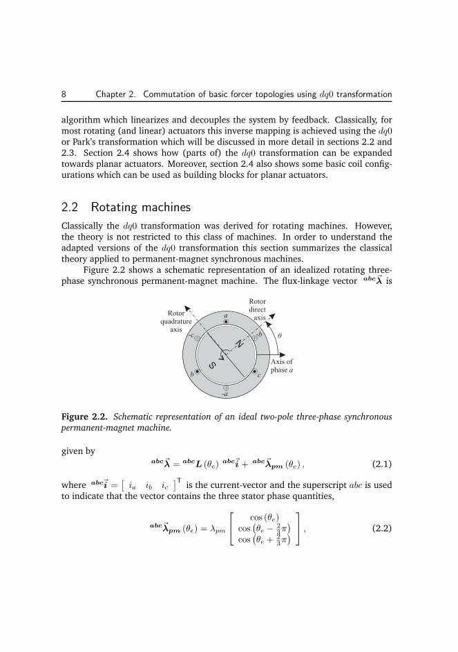
Figure 2.2 shows a schematic representation of an idealized rotating three-phase synchronous permanent-magnet machine. The flux-linkage vector abc~λ is
Figure 2.2. Schematic representation of an ideal two-pole three-phase synchronous
permanent-magnet machine.
given byabc~λ = abcL (θe)
abc~i + abc~λpm (θe) , (2.1)
where abc~i =[
ia ib ic]T
is the current-vector and the superscript abc is usedto indicate that the vector contains the three stator phase quantities,
abc~λpm (θe) = λpm
cos (θe)cos(
θe − 23π)
cos(
θe + 23π)
, (2.2)
2.2. Rotating machines 9
is the permanent-magnet flux-linkage vector (the magnets are modeled as ideal fluxsources) and
abcL (θe) =
Laa (θe) Lab (θe) Lac (θe)Lba (θe) Lbb (θe) Lbc (θe)Lca (θe) Lcb (θe) Lcc (θe)
, (2.3)
is the matrix containing the self and mutual inductances of the stator coils. Ideally,the self and mutual inductances can be written as,
Laa = Lself + Lsalient cos (2θe) ,Lbb = Lself + Lsalient cos
(
2θe + 23π)
,Lcc = Lself + Lsalient cos
(
2θe − 23π)
,Lab = Lba = Lmutual + Lsalient cos
(
2θe − 23π)
,Lbc = Lcb = Lmutual + Lsalient cos (2θe) ,Lca = Lac = Lmutual + Lsalient cos
(
2θe + 23π)
,
(2.4)
(resulting in diagonal, θe independent, inductances after applying the dq0-trans-formation which will be explained later in this section) where Lself and Lmutualare the constant parts of the self and mutual inductances, respectively, and Lsalientis an inductance term which is caused by saliency of the rotor depending on theelectrical rotor angle θe
θe =#poles
2θ, (2.5)
(e.g. in figure 2.2 the #poles = 2). The voltage equations are
abc~u = R abc~i +d abc~λ (θe)
dt. (2.6)
A useful method to analyze these machines is to make use of the direct- andquadrature-axis (dq0) theory. The theory uses the concept of resolving synchronous-machine armature quantities into two rotating components: The first component iscalled the direct-axis component, which is aligned with the direction of the rotormagnetization (in the case of permanent-magnet machines). The second compo-nent is called the quadrature component, which is in quadrature with (i.e. orthogo-nal to) the direct axis. Both components are shown in figure 2.2. The original ideabehind this transformation (the Blondel two-reaction method) is derived from thework of A.E. Blondel in France. The transformation was further developed by R.E.Doherty and C.A. Nickle [8, 9, 10, 11] and by R.H. Park [33, 34]. The vector/matrixnotations of the dq0 transformation used in this section are in accordance with [13].A few assumptions have been made for this method to be valid. The following is
10 Chapter 2. Commutation of basic forcer topologies using dq0 transformation
quoted from [33]: ”Attention is restricted to symmetrical three-phase machineswith field structure symmetrical about the axes of the field winding and interpo-lar space, but salient poles and an arbitrary number of rotor circuits is considered.Idealization is resorted to, to the extent that saturation and hysteresis in everymagnetic circuit and eddy currents in the armature iron are neglected, and in theassumption that, as far as concerns effects depending on the position of the rotor,each armature winding may be regarded as, in effect, sinusoidally distributed.” Thepower-invariant transformation is given by
SdSqS0
=2
3
cos(θe) cos(θe − 23π) cos(θe + 2
3π)− sin(θe) − sin(θe − 2
3π) − sin(θe + 23π)
12
12
12
SaSbSc
, (2.7)
where S represents an instantaneous stator quantity to be transformed (e.g. cur-rent, voltage or flux), the subscripts a, b and c represent the three stator phases,respectively, the subscripts d and q represent the direct and quadrature axes, respec-tively, and θe is the electrical angle given by (2.5). The inverse dq0 transformationis given by
SaSbSc
=
cos(θe) − sin(θe) 1cos(θe − 2
3π) − sin(θe − 23π) 1
cos(θe + 23π) − sin(θe + 2
3π) 1
SdSqS0
. (2.8)
The third component, indicated by subscript 0, is added to the d and q compo-nents to create a unique transformation of the three stator phase components. Fornotational simplicity (2.7) and (2.8) are written as
dq0~s = dq0T abc (θe)abc~s, (2.9)
andabc~s = abcT dq0 (θe)
dq0~s, (2.10)
respectively.When applying the transformation to the flux linkages described by (2.1) the
following result is obtained
dq0~λ = dq0L dq0~i + dq0~λpm, (2.11)
where
dq0L = dq0T abc (θe)abcL (θe)
abcT dq0 (θe) =
Ld 0 00 Lq 00 0 L0
, (2.12)
2.2. Rotating machines 11
and
dq0~λpm = dq0T abc (θe)abc~λpm (θe) =
λpm00
, (2.13)
are now independent of the electrical rotor angle θe. The direct-axis and quadrature-axis synchronous inductances Ld and Lq, and the zero-sequence inductance L0 areequal to
Ld = Lself − Lmutual +32Lsalient,
Lq = Lself − Lmutual − 32Lsalient,
L0 = Lself + 2Lmutual.(2.14)
Transformation of the voltage equations (2.6) results in
dq0~u = dq0T abc (θe)(
R abcT dq0 (θe)dq0~i +
d abcT dq0(θe)dq0~λ
d t
)
= R dq0~i + dq0Ld dq0~id t + ∂θe
∂t
0 −1 01 0 00 0 0
dq0~λ,(2.15)
where
dq0~usv =∂θe∂t
0 −1 01 0 00 0 0
dq0~λ, (2.16)
is the speed-voltage term. The instantaneous power ps then becomes
ps = abc~uT abc~i = dq0~uTabcT dq0 (θe)T abcT dq0 (θe)
dq0~i
= 32
dq0~uT
1 0 00 1 00 0 2
dq0~i.(2.17)
The electromagnetic torque, Tmech, is obtained by dividing the power output corre-sponding to the speed-voltage term by the mechanical speed dθ
dt
Tmech = 32
(
dθdt
)−1 ∂θe∂t
dq0~λT
0 1 0−1 0 00 0 0
dq0~i
= 32
(
#poles2
)
(λpmiq + (Ld − Lq) idiq) .
(2.18)
For three-phase two-pole synchronous permanent-magnet machines without saliency(Ld = Lq and θe = θ) as in figure 2.2, equation 2.18 can be simplified to
Tmech = 32λpmiq . (2.19)
12 Chapter 2. Commutation of basic forcer topologies using dq0 transformation
2.3 Linear actuators
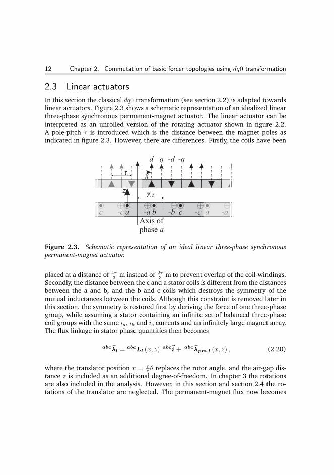
In this section the classical dq0 transformation (see section 2.2) is adapted towardslinear actuators. Figure 2.3 shows a schematic representation of an idealized linearthree-phase synchronous permanent-magnet actuator. The linear actuator can beinterpreted as an unrolled version of the rotating actuator shown in figure 2.2.A pole-pitch τ is introduced which is the distance between the magnet poles asindicated in figure 2.3. However, there are differences. Firstly, the coils have been
Figure 2.3. Schematic representation of an ideal linear three-phase synchronous
permanent-magnet actuator.
placed at a distance of 4τ3 m instead of 2τ
3 m to prevent overlap of the coil-windings.Secondly, the distance between the c and a stator coils is different from the distancesbetween the a and b, and the b and c coils which destroys the symmetry of themutual inductances between the coils. Although this constraint is removed later inthis section, the symmetry is restored first by deriving the force of one three-phasegroup, while assuming a stator containing an infinite set of balanced three-phasecoil groups with the same ia, ib and ic currents and an infinitely large magnet array.The flux linkage in stator phase quantities then becomes
abc~λl = abcLl (x, z) abc~i + abc~λpm,l (x, z) , (2.20)
where the translator position x = τπ θ replaces the rotor angle, and the air-gap dis-
tance z is included as an additional degree-of-freedom. In chapter 3 the rotationsare also included in the analysis. However, in this section and section 2.4 the ro-tations of the translator are neglected. The permanent-magnet flux now becomes
2.3. Linear actuators 13
[17]
abc~λpm,l (x, z) = λpm exp(
−πτz)
cos(
πτ x)
cos(
πτ x+ 2
3π)
cos(
πτ x− 2
3π)
. (2.21)
Ideally, the self and mutual inductances of the three stator coils then become
Laa,l = Lself,l (z) + Lsalient,l (z) cos(
2πτ x)
,Lbb,l = Lself,l (z) + Lsalient,l (z) cos
(
2πτ x− 23π)
,Lcc,l = Lself,l (z) + Lsalient,l (z) cos
(
2πτ x+ 23π)
,Lab,l = Lba,l = L∗
mutual,l (z) + Lsalient,l (z) cos(
2πτ x+ 23π)
,
Lbc,l = Lcb,l = L∗mutual,l (z) + Lsalient,l (z) cos
(
2πτ x)
,
Lca,l = Lac,l = L∗mutual,l (z) + Lsalient,l (z) cos
(
2πτ x− 23π)
,
(2.22)
where L∗mutual,l (z) is the effective mutual inductance including the mutual induc-
tances of the neighboring balanced three-phase groups operating at the same cur-rents (to maintain the same symmetry as with the rotating machine).
The following derivation is comparable to the work of Won-Jon Kim [29]. Thedq0 transformation dq0T abc,l (x) and its inverse transformation abcT dq0,l (x) havebeen adapted to match the linear actuator as follows
dq0T abc,l (x) =2
3
cos(πτ x) cos(πτ x+ 23π) cos(πτ x− 2
3π)− sin(πτ x) − sin(πτ x+ 2
3π) − sin(πτ x− 23π)
12
12
12
, (2.23)
abcT dq0,l (x) =
cos(πτ x) − sin(πτ x) 1cos(πτ x+ 2
3π) − sin(πτ x+ 23π) 1
cos(πτ x− 23π) − sin(πτ x− 2
3π) 1
. (2.24)
When applying the transformations given by (2.23) and (2.24) to the linear ac-tuator, comparable results are obtained as with the rotating actuator described insection 2.2. The main differences are that after transformation the inductance ma-trix dq0Ll and the permanent magnet flux dq0~λpm,l have become z dependent, asfollows
Ld(z) = Lself,l(z) − L∗mutual,l(z) + 3
2Lsalient,l(z),
Lq(z) = Lself,l(z) − L∗mutual,l(z) − 3
2Lsalient,l(z),
L0(z) = Lself,l(z) + 2L∗mutual,l(z),
(2.25)
dq0~λpm,l(z) = exp(
−πτz)
λpm00
. (2.26)
14 Chapter 2. Commutation of basic forcer topologies using dq0 transformation
The z dependency results in an additional speed-voltage term. The speed-voltageterms in dq0 coordinates are
dq0~usv,x =π
τ
∂x
∂t
0 −1 01 0 00 0 0
dq0~λ(z), (2.27)
and
dq0~usv,z =∂z
∂t
(
∂ dq0Ll(z)
∂zdq0~il +
∂ dq0~λpm,l(z)
∂z
)
. (2.28)
The electromagnetic forces, Fx,l and Fz,l, are again obtained by dividing the poweroutput corresponding to the speed-voltage term by the mechanical speeds dx
dt anddzdt , respectively
Fx,l = 32πτ
dq0~λT
l (z)
0 1 0−1 0 00 0 0
dq0~i
= 32πτ
(
λpm,l exp(
−πτ z)
iq + (Ld(z) − Lq(z)) idiq)
,
(2.29)
Fz,l = 32
(
dq0~iT
l∂ dq0LT
l (z)∂z +
∂ dq0~λpm,l(z)∂z
)
1 0 00 1 00 0 2
dq0~il
= 32
(
∂Ld(z)∂z i2d +
∂Lq(z)∂z i2q + 2∂L0(z)
∂z i20 − πτ λpm,l exp
(
−πτ z)
id
)
.
(2.30)
Without saliency of the translator (Ld = Lq), the force in the x-direction Fx,l sim-plifies to:
Fx,l =3
2
π
τλpm,l exp
(
−πτz)
iq . (2.31)
When all materials are considered to have a relative permeability µr equal to one(no reluctance forces) the force in the z-direction Fz,l simplifies to
Fz,l = −3
2
π
τλpm,l exp
(
−πτz)
id . (2.32)
Moreover, when assuming all materials to have µr = 1 and ideal current amplifiers,it is not only possible to analyze the linear actuator as a Lorentz actuator (sincethe force calculation through the flux linkage and the Lorentz force are equivalentfor a current loop in an external magnetic field [12]), but the need for symmetry
2.3. Linear actuators 15
is also removed. The dq0-transformation can still be effectively applied to linearizeand decouple the permanent-magnet flux linkage abc~λpm,l (x, z). When (2.20) isapplied to the voltage equations and (2.24) is applied to the permanent magnetflux linkage abc~λpm,l (x, z) the following result is obtained
abc~ul = R abc~il + abcLl
d abc~il
dt+ abc~usv,x + abc~usv,z, (2.33)
where abcLl is position independent and where abc~usv,x and abc~usv,z are givenby
abc~usv,x =∂x
∂t
∂ abcT dq0,l (x)
∂xdq0~λpm,l (z) , (2.34)
abc~usv,z =∂z
∂tabcT dq0,l (x)
∂ dq0~λpm,l (z)
∂z. (2.35)
The electromagnetic forces, Fx,l and Fz,l, then become equal to (2.31) and (2.32),respectively. It is then possible to linearize and decouple the forces by feedbackusing the inverse mapping of (2.31) and (2.32)
dq0~ides,l =2
3
τ
π
1
λpm,lexp
(π
τz)
0 −11 00 0
[
Fdesx,lFdesz,l
]
, (2.36)
or in the real abc stator frame currents
abc~ides,l =2
3
τ
π
1
λpm,lexp
(π
τz)
abcT dq0,l (x)
0 −11 00 0
[
Fdesx,lFdesz,l
]
. (2.37)
The current on the zero axis i0 can have an arbitrary value since it does not con-tribute to the force production. In (2.36), however, i0 is set to zero in order tominimize the power dissipation (which can be seen from (2.17)).
The transformation described above is not limited to three-phase systems. Fig-ure 2.4 shows a semi-four-phase actuator (a four-phase actuator of which only thefirst and the second or fourth phase are used). The transformation matrices thenbecome
dqT ab,l (x) = abT dq,l (x) =
[
cos(πτ x) − sin(πτ x)− sin(πτ x) − cos(πτ x)
]
, (2.38)
where there is no 0-axis anymore because the matrix is already uniquely defined.The currents can then be derived equivalent to the derivation of (2.37), resulting in
ab~ides,l =τ
π
1
λpm,lexp
(π
τz)
abT dq,l (x)
[
0 −11 0
] [
Fdesx,lFdesz,l
]
. (2.39)
16 Chapter 2. Commutation of basic forcer topologies using dq0 transformation
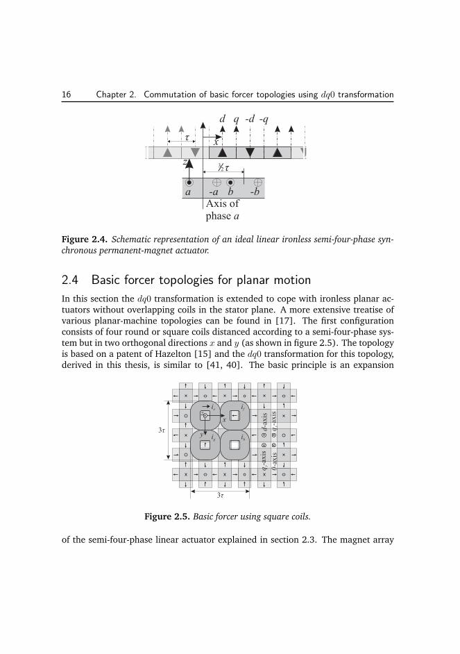
Figure 2.4. Schematic representation of an ideal linear ironless semi-four-phase syn-
chronous permanent-magnet actuator.
2.4 Basic forcer topologies for planar motion
In this section the dq0 transformation is extended to cope with ironless planar ac-tuators without overlapping coils in the stator plane. A more extensive treatise ofvarious planar-machine topologies can be found in [17]. The first configurationconsists of four round or square coils distanced according to a semi-four-phase sys-tem but in two orthogonal directions x and y (as shown in figure 2.5). The topologyis based on a patent of Hazelton [15] and the dq0 transformation for this topology,derived in this thesis, is similar to [41, 40]. The basic principle is an expansion
Figure 2.5. Basic forcer using square coils.
of the semi-four-phase linear actuator explained in section 2.3. The magnet array
2.4. Basic forcer topologies for planar motion 17
shown in figure 2.5 is called a Halbach magnet array which is used to increase andconcentrate the magnetic flux density near the coils. The topology has two q-axes:One axis belonging to the x-direction and one belonging to the y-direction, calledqx and qy, respectively. The dqxqy0 transformation matrices belonging to figure 2.5are given by
dqxqy0T efgh = efghT dqxqy0 =
c(
πxτ
)
c(
πyτ
)
−s(
πxτ
)
c(
πyτ
)
−c(
πxτ
)
s(
πyτ
)
s(
πxτ
)
s(
πyτ
)
−s(
πxτ
)
c(
πyτ
)
−c(
πxτ
)
c(
πyτ
)
s(
πxτ
)
s(
πyτ
)
c(
πxτ
)
s(
πyτ
)
−c(
πxτ
)
s(
πyτ
)
s(
πxτ
)
s(
πyτ
)
−c(
πxτ
)
c(
πyτ
)
s(
πxτ
)
c(
πyτ
)
s(
πxτ
)
s(
πyτ
)
c(
πxτ
)
s(
πyτ
)
s(
πxτ
)
c(
πyτ
)
c(
πxτ
)
c(
πyτ
)
,(2.40)
which are orthonormal matrices (where for notational simplicity sin and cos havebeen replaced by s and c, respectively). The three speed-voltage terms then become
efgh~usv,x =∂x
∂t
∂ efghT dqxqy0 (x, y)
∂xdq0~λpm,pl (z) , (2.41)
efgh~usv,y =∂y
∂t
∂ efghT dqxqy0 (x, y)
∂ydq0~λpm,pl (z) , (2.42)
and
efgh~usv,z =∂z
∂tefghT dqxqy0 (x, y)
∂ dq0~λpm,pl (z)
∂z, (2.43)
with their respective force components
Fx =π
τλpm exp
(
−√
2π
τz
)
iqx , (2.44)
Fy =π
τλpm exp
(
−√
2π
τz
)
iqy , (2.45)
Fz = −√
2π
τλpm exp
(
−√
2π
τz
)
id. (2.46)
(2.47)
18 Chapter 2. Commutation of basic forcer topologies using dq0 transformation
The currents which can be used to linearize and decouple the system then become
efgh~ides =τ
π
1
λpmexp
(√2π
τz
)
efghT dqxqy0 (x, y)
0 0 −√
22
1 0 00 1 00 0 0
FdesxFdesyFdesz
.
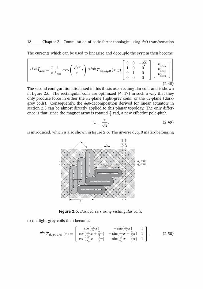
(2.48)The second configuration discussed in this thesis uses rectangular coils and is shownin figure 2.6. The rectangular coils are optimized [4, 17] in such a way that theyonly produce force in either the xz-plane (light-grey coils) or the yz-plane (dark-grey coils). Consequently, the dq0-decomposition derived for linear actuators insection 2.3 can be almost directly applied to this planar topology. The only differ-ence is that, since the magnet array is rotated π
4 rad, a new effective pole-pitch
τn =τ√2, (2.49)
is introduced, which is also shown in figure 2.6. The inverse dxqx0 matrix belonging
Figure 2.6. Basic forcers using rectangular coils.
to the light-grey coils then becomes
abcT dxqx0,pl (x) =
cos( πτnx) − sin( πτnx) 1
cos( πτnx+ 23π) − sin( πτnx+ 2
3π) 1
cos( πτnx− 23π) − sin( πτnx− 2
3π) 1
, (2.50)
2.4. Basic forcer topologies for planar motion 19
which results in the following currents for the light-grey coils
abc~ides,pl =2
3
τnπ
1
λpm,lexp
(
π
τnz
)
abcT dxqx0,l (x)
0 −11 00 0
[
Fdesx,plFdesz,pl
]
.
(2.51)A similar solution can be obtained for the dark-grey coils (where x is substituted byy).

20 Chapter 2. Commutation of basic forcer topologies using dq0 transformation
Chapter 3
Linearization and decoupling
of the wrench
3.1 Introduction
Contrary to chapter 2, where the dq0 transformation was used to derive a decou-pling strategy of the force components, this chapter focusses on a six degree-of-freedom approach towards solving the commutation algorithm. Classical dq0 trans-formation can only be used directly to derive a commutation which decouples theforce components of linear/planar actuators. In moving-coil planar actuators suchas [5] it is possible to use design symmetries which reduce the complexity of thetorque equations, therefore, additional transformations can be derived which al-low for decoupling of the torque [4]. Moving-magnet planar actuators with inte-grated magnetic bearing have complex torque equations. The result of these com-plex torque equations is that the classical dq0-transformation, which focusses on theforce components (when applied to planar actuators), is not practical to use sinceit does not directly include torque decoupling. In literature, attempts have beenmade to include decoupling of the torque by using additional transformations afterapplying dq0-transformation [41, 40]. However, the resulting disturbance torqueremained significant. In patent literature some improvements to the algorithmshave been made by Binnard et al. [1, 2] resulting in a six DOF algorithm whichstill does not include the full torque equations. Moreover, since only the coils un-derneath or near the edges of the translator significantly produce force and torque,the set of active coils which are used to control the translator needs to change as afunction of position. There are no explicit solutions given in [1, 2] which allow forswitching of active coil sets without disturbing the decoupling.
21
22 Chapter 3. Linearization and decoupling of the wrench
The approach which is proposed in section 3.3 uses the six degree-of-freedommodel derived in section 3.2 to achieve a direct wrench-current decoupling which,in contrast to the dq0 transformation, directly decouples the force and torque com-ponents. Moreover, section 3.3.1 expands the algorithm to include switching ofactive coil sets. The method presented in this thesis has also been published [44,42, 43, 25]. The commutation algorithms and the real-time model derived in thischapter are the results of common research work of project partner ir. J.W. Jansenand the author of this thesis. As a result, these subjects are described in both theses.This thesis summarizes the real-time modeling results. A more extensive treatise onthe electromechanical analysis and design, including more accurate models of thesystem, can be found in [17]. The models discussed in both theses were also pub-lished [24, 26, 22, 18, 23]. Section 3.4 uses the Schur complement to split thedirect wrench-current decoupling into several components. Under certain assump-tions, one of these components can be made equivalent to the sum of multiple dq0transformations which where presented in section 2.4 (also published in [45, 46]).
3.2 Real-time analytical six degree-of-freedom coil model
The dq0 decomposition explained in chapter 2 can only be used directly to decoupleforces (when applied to planar actuators). The reason for this is that the forcedistribution of the planar actuator is not taken into account. However, to accuratelystabilize a platform in six degrees of freedom it is also necessary to control thetorque about the center of mass. To do so a real-time six degree-of-freedom singlecoil model is derived in this section.
When assuming ideal magnets, quasi-static magnetic fields, negligible eddycurrents, a wire diameter smaller than the skin depth, rigid body dynamics of thetranslator and no reluctance forces, the voltage equations can be simplified to
~u = R~i + Ld~i
d t+ J~Λm
(~q)d~q
d t, (3.1)
where J~Λm(~q) is the Jacobian of the flux of the permanent-magnet array linked by
the respective coils, ~q is the 6-DOF vector consisting of the three position and threeorientation components of the translator and R and L are the coils resistance andinductance matrices, respectively. Moreover, when assuming ideal current ampli-fiers, having an infinitely large internal resistance and bandwidth, and no coggingforces, the wrench vector (containing all force and torque components) is thengiven by
~wtot = J~Λm(~q)~i. (3.2)
3.2. Real-time analytical six degree-of-freedom coil model 23
Since the force calculation through the flux linkage and the Lorentz force are equiv-alent for a current loop in an external magnetic field [12], the voltage equationscan be solved with the force and torque calculated using magnetostatic models (i.e.using the Lorentz force and torque).
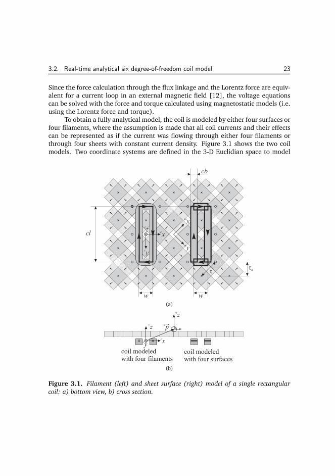
To obtain a fully analytical model, the coil is modeled by either four surfaces orfour filaments, where the assumption is made that all coil currents and their effectscan be represented as if the current was flowing through either four filaments orthrough four sheets with constant current density. Figure 3.1 shows the two coilmodels. Two coordinate systems are defined in the 3-D Euclidian space to model
Figure 3.1. Filament (left) and sheet surface (right) model of a single rectangular
coil: a) bottom view, b) cross section.
24 Chapter 3. Linearization and decoupling of the wrench
the actuator. Figure 3.1 shows a partial planar actuator, i.e. a Halbach permanent-magnet array and a single coil. A coordinate system is located at the stationarypart of the actuator. In this coordinate system the stator coils are defined. For thatreason it is denoted with the superscript c (of coils)
c~x =[
cx cy cz]T. (3.3)
Another coordinate system is fixed to the mass center point of the total translator(although figure 3.1 only shows the permanent magnets). In this coordinate systemthe magnets are defined. This coordinate frame is denoted with the superscript m(of magnets)
m~x =[
mx my mz]T. (3.4)
The vectorc~p =
[
cpxcpy
cpz]T, (3.5)
is the position of the magnet coordinate system m, i.e. the mass center point of thetranslator, in the coil coordinate system c.
Coordinates are transformed from one system to the other with an orientationtransformation and afterwards a translation. The transformation matrix c
Tm for aposition from the magnet to the coil coordinate system is equal to [31]
cTm =
[
cRm
c~p0 1
]
. (3.6)
For convenience, the orientation transformation matrix is defined as
cRm = Rot(cy, θ)Rot(cx, ψ)Rot(cz, φ), (3.7)
where
Rot(cy, θ) =
cos (θ) 0 sin (θ)0 1 0
− sin (θ) 0 cos (θ)
, (3.8)
Rot(cx, ψ) =
1 0 00 cos (ψ) − sin (ψ)0 sin (ψ) cos (ψ)
, (3.9)
Rot(cz, φ) =
cos (φ) − sin (φ) 0sin (φ) cos (φ) 0
0 0 1
, (3.10)
3.2. Real-time analytical six degree-of-freedom coil model 25
and where ψ, θ and φ are the (Euler) rotation angles about the cx- cy-, and cz-axes,respectively. Thus, the position and orientation of the translator can be describedin six degrees-of-freedom. The transformation matrix m
Tc for a position from theglobal to the local coordinate system is equal to
mTc = c
Tm−1 =
[
cRm
T −cRm
Tc~p0 1
]
=
[
mRc −m
Rcc~p
0 1
]
,(3.11)
because cTm is orthonormal.
Applying the appropriate transformation matrix, a position is transferred be-tween the coordinate systems, according to
[
m~x1
]
= mTc
[
c~x1
]
, (3.12)
m~x = mRc (c~x− c~p) , (3.13)
and a free vector as defined in [31], e.g. the spatial current vector ~i (consisting ofthe directional components of the current along the x, y and z directions), accordingto
[
m~i0
]
= mTc
[
c~i0
]
, (3.14)
m~i = mRc
c~i. (3.15)
The analytical model, applied here, only takes the first harmonic of the mag-netic flux density distribution of the permanent-magnet array into account. Thesimplified magnetic flux density expression (assuming the coils are located under-neath the permanent-magnet array) is given by
m ~B3 ( m~x) = − exp
(
π√
2
τmz
)
Bxy cos(
πmxτ
)
sin(
πmyτ
)
Bxy sin(
πmxτ
)
cos(
πmyτ
)
Bz sin(
πmxτ
)
sin(
πmyτ
)
, (3.16)
where Bxy and Bz are derived from the amplitudes of the mean value of the firstharmonic of the magnetic flux density components over the cross section of the coilat mz = 0. Transformation of this expression into the coordinate system of the coils
c ~B3 ( c~x, c~p) = cRm
m ~B3 (mRc ( c~x − c~p)) , (3.17)
26 Chapter 3. Linearization and decoupling of the wrench
results for (φ = −π/4 rad and ψ = θ = 0 rad) in
c ~B3 ( c~x, c~p)∣
∣
∣ψ=θ=0ψ=−π/4
=
−Bxy√2
exp(
πτn
(cz − cpz))
sin(
πτn
(cx− cpx))
Bxy√2
exp(
πτn
(cz − cpz))
sin(
πτn
(cy − cpy))
12Bz exp
(
πτn
(cz − cpz))(
cos(
πτn
(cx− cpx))
− cos(
πτn
(cy − cpx)))
,
(3.18)where a new pole pitch τn is introduced, which is indicated in figure 3.1
τn =τ√2. (3.19)
The Lorentz force on the filaments is calculated by solving a line integral. The
force exerted on the translator c~F =[
cFxcFy
cFz]T
, expressed in the coil
coordinate system, by one coil, which is located at c~x =[
cx cy 0]T
, is equalto
c~F = −∮
Cc~i × c ~B3dl =
−∫cx+w/2cx−w/2 [i 0 0]
T × c ~B3
(
[cx′ cy − cl/2 0]T, c~p
)
dcx′
−∫cy+cl/2cy−cl/2 [0 i 0]
T × c ~B3
(
[cx+ w/2 cy′ 0]T, c~p
)
dcy′
−∫cx+w/2cx−w/2 [−i 0 0]
T × c ~B3
(
[cx′ cy + cl/2 0]T, c~p
)
dcx′
−∫cy+cl/2cy−cl/2 [0 − i 0]
T × c ~B3
(
[cx− w/2 cy′ 0]T, c~p
)
dcy′,
(3.20)
where w and cl are the sizes of the filament coil along the cx- and cy-directions,respectively, and i is the current through the coil in Ampere-turns.
The torque exerted on the translator c~T =[
cTxcTy
cTz]T
, expressedin the global coordinate system, by the same coil is equal to
c~T = −∮
C ( c~x − c~p) ×(
c~i × c ~B3
)
dl =
−∫cx+w/2cx−w/2 (c~x − c~p)×
(
[i 0 0]T× c ~B3
(
[cx′ cy − cl/2 0]T, c~p
))
dcx′
−∫cy+cl/2cy−cl/2 (c~x − c~p)×
(
[0 i 0]T× c ~B3
(
[cx+ w/2 cy′ 0]T, c~p
))
dcy′
−∫cx+w/2cx−w/2 (c~x − c~p)×
(
[−i 0 0]T× c ~B3
(
[cx′ cy + cl/2 0]T, c~p
))
dcx′
−∫cy+cl/2cy−cl/2 (c~x − c~p)×
(
[0 −i 0]T× c ~B3
(
[cx− w/2 cy′ 0]T, c~p
))
dcy′.
(3.21)
3.2. Real-time analytical six degree-of-freedom coil model 27
The force and torque exerted on the translator (here expressed in coil coordinatesc) are modeled as the reaction force and torque of the force and torque exertedon the coil. Hence, the minus signs in (3.21) and (3.20). If the length of the coilcl = 2nτn, where n is an integer, and if φ = −π/4 rad and ψ = θ = 0 rad, the coilonly produces force in the cx- and cz-directions and the force is independent on thecpy-position of the magnet array. The force and torque expressions for a coil withw = τn and cl = 4τn are given by
cFx = −2√
2Bziτ exp
(
− π
τncpz
)
sin
(
π
τn(cpx − cx)
)
, (3.22)
cFy = 0, (3.23)
cFz = −4Bxyiτ exp
(
− π
τncpz
)
cos
(
π
τn(cpx − cx)
)
, (3.24)
cTx = (cy − cpy)cFz −Bxyiτ
2 exp
(
− π
τncpz
)
sin
(
π
τn(cpy − cy)
)
, (3.25)
cTy = (cpx − cx) cFz − cpzcFx, (3.26)
cTz = cFx (cpy − cy) . (3.27)
In [17] it is derived thatBz =
√2Bxy, (3.28)
which results in equal amplitudes of the cx- and cz-components of the force. Thetorque component cTx cannot be expressed as an arm multiplied by a force. There-fore, a single attaching point of the force in the cy-direction cannot be defined.Hence, for accurate torque calculation, the distribution of the force over the coilshould be taken into account. Note that the cross-product with the arm, which isadded in the line integral of the torque equation of the filament coil model (3.21),is inside the integral in order to include the force distribution over the coil. Thecoil model with four filaments assumes that the force can be modeled to act on thecenter of the conductor bundle. In reality, the distribution of the force over theconductor bundle changes with the relative position of the coil with respect to themagnet array. This can be shown by modeling the conductor bundle with a sheet orsurface current. The obtained force and torque expressions for a coil with w = τn,cl = 4τn and a conductor bundle width cb = τn/2 and (φ = −π/4 rad and ψ = θ = 0rad) are similar to the expressions for the coil modeled with four filaments, exceptfor the cTy term
cTy = (cpx − cx) cFz − cpzcFx +c Fx
Bxy (π − 4) τ
4Bzπ, (3.29)
28 Chapter 3. Linearization and decoupling of the wrench
cTy contains an extra term proportional to cFx, which represents the torque causedby the change of the attaching point of the force in the conductor bundle of thecoil. In further analyses in this thesis and in the controller of the realized planaractuator, the model based on the sheet currents is used. The reason for this is thehigher accuracy of the torque model (as can be seen from the difference between(3.26) and (3.29)).
For notational simplicity the force and torque components are combined in a
single wrench vector l ~wn =[
cFxcFy
cFzcTx
cTycTz
]TThe wrench
vector l ~wn of a single coil n can then be described by
l ~wn = ~γn
(
l~q , l~rn
)
lin, (3.30)
where in is the current through the nth coil, ~γn is the vector mapping the current to
the wrench vector, l~q =[
cpxcpy
cpz ψ θ φ]T
is the vector containingthe position and orientation of the mass center point of the translator with respectto its reference frame in local coil coordinates (indicated by superscript l which is
properly defined in section 3.3.1) and l~rn =[
cx cy φ]T
is the location andorientation of the nth coil in the xy-plane with respect to the origin of the localcoil coordinates (where from this point cz = 0). Since the model neglects the edgeeffects of the magnet array it is only valid when the coil is underneath the translator.Let Sn be the set of admissible coordinates l~q for the model of the nth coil to bevalid. Figure 3.2 shows a top-view of coil n (where both a square/round coil andthe rectangular coil is shown since both are used in this thesis) with the admissibleset of l~qn coordinates about a given coil location l~rn defined as Sn. The centerof set Sn is, therefore, depending on the l~rn location while the size of the set isdetermined by the size of the magnet-array. When the edge effects of the magnetarray are included in the model, the size of this set can be increased.
When assuming rigid body behavior, superposition of coil currents can be ap-plied to obtain the total wrench on the center of mass of the translator
l ~wtot =
m∑
n=1
~γn
(
l~q , l~rn
)
lin, (3.31)
or in matrix form
l ~wtot =[
~γ1
(
l~q , l~r1
)
· · · ~γm−1
(
l~q , l~rm−1
)
~γm
(
l~q , l~rm
) ]
l~i, (3.32)
where l~r1 · · · l~rm are the vectors containing the position and orientation infor-mation of each of the coils and l~i is a vector consisting of all active coil currents
3.3. Direct wrench-current decoupling 29
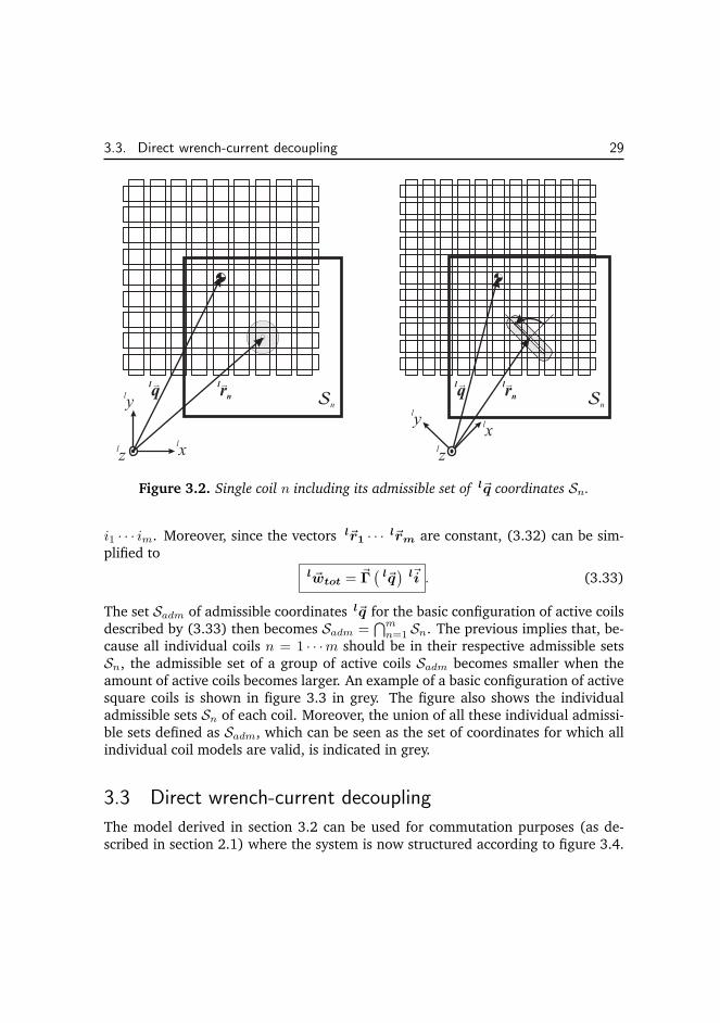
Figure 3.2. Single coil n including its admissible set of l~q coordinates Sn.
i1 · · · im. Moreover, since the vectors l~r1 · · · l~rm are constant, (3.32) can be sim-plified to
l ~wtot = ~Γ(
l~q)
l~i . (3.33)
The set Sadm of admissible coordinates l~q for the basic configuration of active coilsdescribed by (3.33) then becomes Sadm =
⋂mn=1 Sn. The previous implies that, be-
cause all individual coils n = 1 · · ·m should be in their respective admissible setsSn, the admissible set of a group of active coils Sadm becomes smaller when theamount of active coils becomes larger. An example of a basic configuration of activesquare coils is shown in figure 3.3 in grey. The figure also shows the individualadmissible sets Sn of each coil. Moreover, the union of all these individual admissi-ble sets defined as Sadm, which can be seen as the set of coordinates for which allindividual coil models are valid, is indicated in grey.
3.3 Direct wrench-current decoupling
The model derived in section 3.2 can be used for commutation purposes (as de-scribed in section 2.1) where the system is now structured according to figure 3.4.
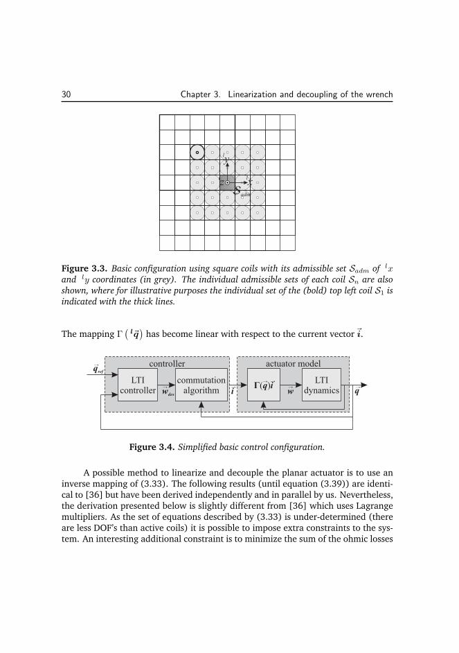
30 Chapter 3. Linearization and decoupling of the wrench
Figure 3.3. Basic configuration using square coils with its admissible set Sadm of lxand ly coordinates (in grey). The individual admissible sets of each coil Sn are also
shown, where for illustrative purposes the individual set of the (bold) top left coil S1 is
indicated with the thick lines.
The mapping Γ(
l~q)
has become linear with respect to the current vector ~i.
Figure 3.4. Simplified basic control configuration.
A possible method to linearize and decouple the planar actuator is to use aninverse mapping of (3.33). The following results (until equation (3.39)) are identi-cal to [36] but have been derived independently and in parallel by us. Nevertheless,the derivation presented below is slightly different from [36] which uses Lagrangemultipliers. As the set of equations described by (3.33) is under-determined (thereare less DOF’s than active coils) it is possible to impose extra constraints to the sys-tem. An interesting additional constraint is to minimize the sum of the ohmic losses
3.3. Direct wrench-current decoupling 31
in the coils
minΓ( l~q) l~i= l ~wdes
∥
∥
∥
l~i∥
∥
∥
2
R=∥
∥Γ− ( l~q
)
l ~wdes
∥
∥
2
R∀ l~q ∈ Sadm, (3.34)
where the ohmic losses are described by∥
∥
∥
l~i∥
∥
∥
2
Rwhich is the squared weighted 2-
norm of the active current vector(
l~iT
Rl~i)
where R is a diagonal weighting matrix
of which the elements correspond to the resistances of each active coil. The matrixΓ− ( l~q
)
is a reflexive generalized inverse of Γ(
l~q)
[37]. Specifically, we make useof the following result
Lemma 3.1. Let ‖~x‖N :=√
~xHN~x, be a (weighted) norm on ~x where N ≻ 0 and let
A~x = ~y. Suppose A has full row rank. Then there exists a linear map A− such that
minA~x=~y
‖~x‖N =∥
∥A−~y∥
∥
N. (3.35)
This map is given by
A− = N
−1A
H(
AN−1
AH)−1
, (3.36)
and satisfies AA− = I, AA
−A = A, (A−
A)HN = NA
−A and is called the
(weighted) minimum norm reflexive generalized inverse (or weak generalized inverse)
of A.
Proof. The proof is given in [37, section 3.1, theorem 3.1.3]�
The solution to minimization problem (3.34) can be found using lemma 3.1.The dimensions of Γ are #DOF × #coils so the rank of matrix Γ should equal theamount of DOF for the system of equations to be consistent. Furthermore, R is adiagonal matrix so the condition R ≻ 0 holds since all coil resistances are largerthan zero. Therefore,
Γ− ( l~q
)
= R−1
ΓT(
l~q)
(
Γ(
l~q)
R−1
ΓT(
l~q)
)−1
∀ l~q ∈ Sadm. (3.37)
When assuming all resistances to be equal to RL (and positive) (3.34) simplifies to
minΓ( l~q) l~i= l ~wdes
RL
∥
∥
∥
l~i∥
∥
∥
2
= RL∥
∥Γ− ( l~q
)
l ~wdes
∥
∥
2 ∀ l~q ∈ Sadm, (3.38)
32 Chapter 3. Linearization and decoupling of the wrench
and (3.37) simplifies to
Γ− ( l~q
)
= ΓT(
l~q)
(
Γ(
l~q)
ΓT(
l~q)
)−1
∀ l~q ∈ Sadm . (3.39)
where the solution is now independent of RL.
3.3.1 Switching
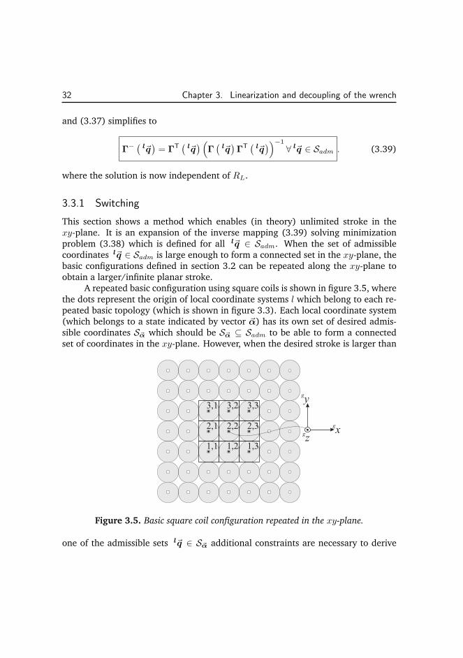
This section shows a method which enables (in theory) unlimited stroke in thexy-plane. It is an expansion of the inverse mapping (3.39) solving minimizationproblem (3.38) which is defined for all l~q ∈ Sadm. When the set of admissiblecoordinates l~q ∈ Sadm is large enough to form a connected set in the xy-plane, thebasic configurations defined in section 3.2 can be repeated along the xy-plane toobtain a larger/infinite planar stroke.
A repeated basic configuration using square coils is shown in figure 3.5, wherethe dots represent the origin of local coordinate systems l which belong to each re-peated basic topology (which is shown in figure 3.3). Each local coordinate system(which belongs to a state indicated by vector ~α) has its own set of desired admis-sible coordinates S~α which should be S~α ⊆ Sadm to be able to form a connectedset of coordinates in the xy-plane. However, when the desired stroke is larger than
Figure 3.5. Basic square coil configuration repeated in the xy-plane.
one of the admissible sets l~q ∈ S~α additional constraints are necessary to derive
3.3. Direct wrench-current decoupling 33
a commutation algorithm. To derive these additional constraints it is necessary tointroduce the voltage equations of the ironless moving-magnet planar actuator
g~u = gR
g~i+ gL
d g~i
d t+
d g ~Λm ( g~q)
d t= g
Rg~i+ g
Ld g~i
d t+J g ~Λm
( g~q)d g~q
d t, (3.40)
where the superscript g denotes the global coordinate system, g~λpm is the vectorcontaining the flux linkage of the flux caused by the permanent magnets linked withthe stator coils, J g ~Λm
is the Jacobian of the flux linkage with respect to the positionand orientation of the permanent-magnet array in global coordinates. The globalcoordinate frame g is introduced to keep track of the global position of the magnetarray with respect to the repeating coil structure in local coil coordinates (e.g. seefigure 3.5 which shows the global coordinates for the square coil topology andthe centers of the nine local coordinate systems which are indicated by the dots).The second term of equation 3.40 depends on the time derivative of the currents.Therefore, since the amplifiers which are used to control the currents through thecoils have a limited voltage range, the current waveforms must be continuous andhave a limited time derivative.
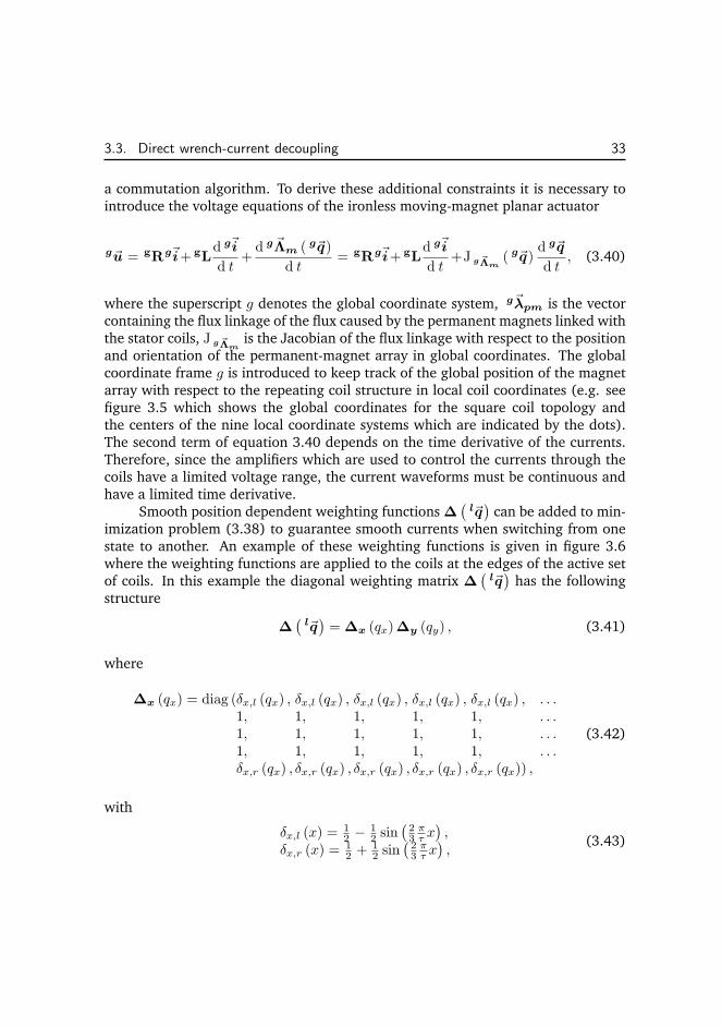
Smooth position dependent weighting functions ∆(
l~q)
can be added to min-imization problem (3.38) to guarantee smooth currents when switching from onestate to another. An example of these weighting functions is given in figure 3.6where the weighting functions are applied to the coils at the edges of the active setof coils. In this example the diagonal weighting matrix ∆
(
l~q)
has the followingstructure
∆(
l~q)
= ∆x (qx)∆y (qy) , (3.41)
where
∆x (qx) = diag (δx,l (qx) , δx,l (qx) , δx,l (qx) , δx,l (qx) , δx,l (qx) , . . .1, 1, 1, 1, 1, . . .1, 1, 1, 1, 1, . . .1, 1, 1, 1, 1, . . .δx,r (qx) , δx,r (qx) , δx,r (qx) , δx,r (qx) , δx,r (qx)) ,
(3.42)
with
δx,l (x) = 12 − 1
2 sin(
23πτ x)
,δx,r (x) = 1
2 + 12 sin
(
23πτ x)
,(3.43)
34 Chapter 3. Linearization and decoupling of the wrench
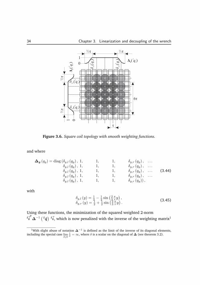
Figure 3.6. Square coil topology with smooth weighting functions.
and where
∆y (qy) = diag (δy,l (qy) , 1, 1, 1, δy,r (qy) , . . .δy,l (qy) , 1, 1, 1, δy,r (qy) , . . .δy,l (qy) , 1, 1, 1, δy,r (qy) , . . .δy,l (qy) , 1, 1, 1, δy,r (qy) , . . .δy,l (qy) , 1, 1, 1, δy,r (qy)) ,
(3.44)
with
δy,l (y) = 12 − 1
2 sin(
23πτ y)
,δy,r (y) = 1
2 + 12 sin
(
23πτ y)
.(3.45)
Using these functions, the minimization of the squared weighted 2-norml~i
T
∆−1(
l~q)
l~i, which is now penalized with the inverse of the weighting matrix1
1With slight abuse of notation ∆−1 is defined as the limit of the inverse of its diagonal elements,
including the special case limδ↓0
1
δ= ∞, where δ is a scalar on the diagonal of ∆ (see theorem 3.2).
3.3. Direct wrench-current decoupling 35
∆(
l~q)
, becomes
minΓ( l~q) l~i= l ~wdes
RL
∥
∥
∥
l~i∥
∥
∥
2
∆−1( l~q)
= RL∥
∥Γ− ( l~q
)
l ~wdes
∥
∥
2
∆−1( l~q)∀ l~q ∈ S~α,
(3.46)
which is now suboptimal with respect to the ohmic losses. The diagonal matrixhas the following property ∆
(
l~q)
� 0. Therefore, the inverse of the diagonal
weighting matrix ∆(
l~q)
is redefined as the inverse of its individual diagonal el-
ements. Elements of the diagonal inverse matrix ∆−1(
l~q)
can, therefore, alsobecome infinitely large. Lemma 3.1 is only valid for positive definite weighting ma-trices and, therefore, it cannot be used directly to derive a solution to minimizationproblem (3.46) when one or more elements of ~δ
(
l~q)
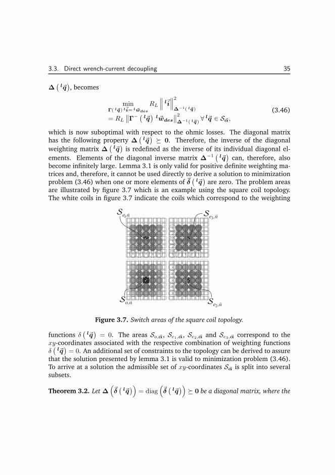
are zero. The problem areasare illustrated by figure 3.7 which is an example using the square coil topology.The white coils in figure 3.7 indicate the coils which correspond to the weighting
Figure 3.7. Switch areas of the square coil topology.
functions δ(
l~q)
= 0. The areas So,~α, Se1,~α, Se2,~α and Se3,~α correspond to thexy-coordinates associated with the respective combination of weighting functionsδ(
l~q)
= 0. An additional set of constraints to the topology can be derived to assurethat the solution presented by lemma 3.1 is valid to minimization problem (3.46).To arrive at a solution the admissible set of xy-coordinates S~α is split into severalsubsets.
Theorem 3.2. Let ∆
(
~δ(
l~q)
)
= diag(
~δ(
l~q)
)
� 0 be a diagonal matrix, where the
36 Chapter 3. Linearization and decoupling of the wrench
real values δ(
l~q)
on the diagonal are, therefore, given by ~δ(
l~q)
≥ ~0. Let So,~α ⊂ S~αbe an open set of admissible coordinates such that ∆
(
~δ(
l~q)
)
≻ 0 (i.e. all weighting
functions δ(
l~q)
are larger than zero).
Furthermore, let S~α = (⋃mn=1 Sen,~α) ∪ So,~α, where m is the number of edge sets
Sen,~α and define an edge set as a connected set of admissible coordinates for which each
possible switching situation results in the same combination of zero weighting functions
δ(
l~q)
in ~δ(
l~q)
(an example of these edge sets is given in figure 3.7). Moreover, let
each edge set n have its own local reduced model Γen
(
l~q)
, belonging to its smaller
set of active coil currents corresponding to all δ(
l~q)
which are non-zero, indicated by
vector l~ien.
Then the solution to the following minimization problem of the squared weighted
2-norm l~iT
∆−1(
l~q)
l~i
minΓ( l~q) l~i= l ~wdes
RL
∥
∥
∥
l~i∥
∥
∥
2
∆−1
(
~δ−1
( l~q))
= RL
∥
∥
∥Γ−(
l~q , ~δ(
l~q)
)
l ~wdes
∥
∥
∥
2
∆−1
(
~δ−1
( l~q)) ∀ l~q ∈ S~α,
(3.47)
which is now suboptimal with respect to the ohmic losses, becomes
Γ− ( l~q
)
= ∆(
l~q)
ΓT(
l~q)
(
Γ(
l~q)
∆(
l~q)
ΓT(
l~q)
)−1
∀ l~q ∈ S~α , (3.48)
provided that the rank of matrix Γ(
l~q)
equals the number of DOF for all l~q ∈ So,~αand that the rank of each reduced model Γen
(
l~q)
also equals the amount of DOF for
all l~q belonging to each corresponding l~q ∈ Sen,~α.
Proof. Using lemma 3.1 the solution to minimization problem (3.47), excluding the
edge sets, equals
Γ− ( l~q
)
= ∆(
l~q)
ΓT(
l~q)
(
Γ(
l~q)
∆(
l~q)
ΓT(
l~q)
)−1
∀ l~q ∈ So,~α, (3.49)
provided that the rank of Γ(
l~q)
equals the number of DOF and ∆−1(
l~q)
≻ 0 for alll~q ∈ So,~α.
The minimization problems of the edge sets can be defined as
minΓen ( l~q) l~ien= l ~wdes
RL
∥
∥
∥
l~ien
∥
∥
∥
2
∆−1
en
(
~δ−1
en( l~q)
)
= RL∥
∥Γen
− ( l~q)
l ~wdes
∥
∥
2
∆−1
en
(
~δ−1
en( l~q)
) ∀ l~q ∈ Sen,~α,(3.50)
3.3. Direct wrench-current decoupling 37
where ∆−1en
(
~δ−1
en
(
l~q)
)
≻ 0 again is a diagonal weighting matrix where the elements
are given by ~δ−1
en
(
l~q)
which are all corresponding non-zero elements of ~δ(
l~q)
. Ac-
cording to lemma 3.1, the solutions of (3.50) are given by
Γ−en
(
l~q , ~δen
)
= ∆en
(
~δen
)
ΓT
en
(
Γen∆en
(
~δen
)
ΓT
en
)−1
∀ l~q ∈ Sen,~α, (3.51)
provided that the rank of Γenequals the amount of DOF for all l~q ∈ Sen,~α.
Let l~ien0 be the vector of coils that are infinitely penalized (in the example
shown in figure 3.7 this is indicated in red for each switching situation) and let ~δen0
be the vector containing the corresponding weighting functions δ(
l~q)
= 0. Let the
vector ~δ(
~δen, ~δen0
)
be constructed out of the elements of the vectors ~δenand ~δen0.
When defining the inverse of a diagonal matrix as the inverse of its individual diagonal
elements δ and using limδ↓0
1δ = ∞, the following assumption can be made
lim~δen0( l~q)↓~0
Γ−(
l~q , ~δ(
~δen, ~δen0
))
= Γ−(
l~q , ~δ(
~δen, ~0))
∀ l~q ∈ Sen,~α, (3.52)
meaning that the limit of the weighting functions of the edge sets going to zero (result-
ing in an infinite penalty on the edge currents l~ien0) should converge. Assuming that
(3.52) holds, the following should also be true
lim~δen0( l~q)↓~0
∥
∥
∥Γ−(
l~q , ~δ(
~δen, ~δen0
))∥
∥
∥
2
∆−1
(
~δ−1(
~δ−1
en,~δ
−1
en0
)) =
∥
∥
∥Γ−(
l~q , ~δ(
~δen, ~0))∥
∥
∥
2
∆−1
(
~δ−1(
~δ−1
en, ~∞
)) ∀ l~q ∈ Sen,~α.(3.53)
Assume that the conditions for (3.51) hold, then (3.52) holds, resulting in the follow-
38 Chapter 3. Linearization and decoupling of the wrench
ing equations
minΓen ( l~q) l~ien= l ~wdes
RL
∥
∥
∥
l~ien
∥
∥
∥
2
∆−1
en
(
~δ−1
en
) =
minΓ( l~q) l~i= l ~wdes
l~ien0=~0
RL
∥
∥
∥
l~ien
∥
∥
∥
2
∆−1
en
(
~δ−1
en
) =
lim~δen0( l~q)↓~0
minΓ( l~q) l~i= l ~wdes
RL
∥
∥
∥
l~i∥
∥
∥
2
∆−1
(
~δ−1(
~δ−1
en,~δ
−1
en0
)) =
lim~δen0( l~q)↓~0
∥
∥
∥Γ−(
l~q , ~δen0
)∥
∥
∥
2
∆−1
(
~δ−1(
~δ−1
en,~δ
−1
en0
)) =
∥
∥
∥Γ−(
l~q , ~0)∥
∥
∥
2
∆−1
(
~δ−1(
~δ−1
en, ~∞
)) =
=∥
∥
∥Γ−(
l~q , ~0)∥
∥
∥
2
∆−1
(
~δ−1(
~δ−1
e0n, ~∞
)) ∀ l~q ∈ Sen,~α.
(3.54)
Given S~α = (⋃mn=1 Sen,~α) ∪ So,~α, where m is the amount of edge sets, this proofs that
(3.48) is the required generalized inverse �
The square coil topology can have an infinite stoke in the xy-plane using thederived commutation algorithm. The algorithm smoothly forces the edge currentsto zero and the structure repeats itself in the xy-plane. This can also be shown bylooking at the hybrid automaton [3] shown in figure 3.8 with the guards (switchingconditions):
Gxp,yp ={{
lqx,lqy}
∈ R2∣
∣lqx >
34τ ∧ lqy >
34τ}
,Gxp =
{{
lqx,lqy}
∈ R2∣
∣lqx >
34τ ∧ − 3
4τ <lqy ≤ 3
4τ}
,Gxp,yn =
{{
lqx,lqy}
∈ R2∣
∣lqx >
34τ ∧ lqy ≤ − 3
4τ}
,Gyn =
{{
lqx,lqy}
∈ R2∣
∣− 34τ <
lqx ≤ 34τ ∧ lqy ≤ − 3
4τ}
,Gxn,yn =
{{
lqx,lqy}
∈ R2∣
∣lqx ≤ − 3
4τ ∧ lqy ≤ − 34τ}
,Gxn =
{{
lqx,lqy}
∈ R2∣
∣lqx ≤ − 3
4τ ∧ − 34τ <
lqy ≤ 34τ}
,Gxn,yp =
{{
lqx,lqy}
∈ R2∣
∣lqx ≤ 3
4τ ∧ lqy >34τ}
,Gyp =
{{
lqx,lqy}
∈ R2∣
∣− 34τ <
lqx ≤ 34τ ∧ lqy >
34τ}
,
(3.55)
and where the reset maps which update the parameters during a switch are given
3.3. Direct wrench-current decoupling 39
by
Rxp,yp ={({
~α−} ,{
~α+}) ,({
l~q−xy
}
,{
l~q+xy
})∣
∣ ~α−, ~α+ ∈ Z2∧
l~q−xy,
l~q+xy ∈ R
2 ∧ ~α+ = ~α− +
[
11
]
∧ l~q+xy = l~q−
xy −[
32τ32τ
]}
,
Rxp ={({
~α−} ,{
~α+}) ,({
l~q−xy
}
,{
l~q+xy
})∣
∣ ~α−, ~α+ ∈ Z2∧
l~q−xy,
l~q+xy ∈ R
2 ∧ ~α+ = ~α− +
[
10
]
∧ l~q+xy = l~q−
xy −[
32τ0
]}
,
Rxp,yn ={({
~α−} ,{
~α+}) ,({
l~q−xy
}
,{
l~q+xy
})∣
∣ ~α−, ~α+ ∈ Z2∧
l~q−xy,
l~q+xy ∈ R
2 ∧ ~α+ = ~α− +
[
1−1
]
∧ l~q+xy = l~q−
xy −[
32τ
− 32τ
]}
,
Ryn ={({
~α−} ,{
~α+}) ,({
l~q−xy
}
,{
l~q+xy
})∣
∣ ~α−, ~α+ ∈ Z2∧
l~q−xy,
l~q+xy ∈ R
2 ∧ ~α+ = ~α− +
[
0−1
]
∧ l~q+xy = l~q−
xy −[
0− 3
2τ
]}
,
Rxn,yn ={({
~α−} ,{
~α+}) ,({
l~q−xy
}
,{
l~q+xy
})∣
∣ ~α−, ~α+ ∈ Z2∧
l~q−xy,
l~q+xy ∈ R
2 ∧ ~α+ = ~α− +
[
−1−1
]
∧ l~q+xy = l~q−
xy −[
− 32τ
− 32τ
]}
,
Rxn ={({
~α−} ,{
~α+}) ,({
l~q−xy
}
,{
l~q+xy
})∣
∣ ~α−, ~α+ ∈ Z2∧
l~q−xy,
l~q+xy ∈ R
2 ∧ ~α+ = ~α− +
[
−10
]
∧ l~q+xy = l~q−
xy −[
− 32τ0
]}
,
Rxn,yp ={({
~α−} ,{
~α+}) ,({
l~q−xy
}
,{
l~q+xy
})∣
∣ ~α−, ~α+ ∈ Z2∧
l~q−xy,
l~q+xy ∈ R
2 ∧ ~α+ = ~α− +
[
−11
]
∧ l~q+xy = l~q−
xy −[
− 32τ
32τ
]}
,
Ryp ={({
~α−} ,{
~α+}) ,({
l~q−xy
}
,{
l~q+xy
})∣
∣ ~α−, ~α+ ∈ Z2∧
l~q−xy,
l~q+xy ∈ R
2 ∧ ~α+ = ~α− +
[
01
]
∧ l~q+xy = l~q−
xy −[
032τ
]}
.
(3.56)The (smooth) general coordinates can be reconstructed from the local coordinatesin the following way
g~qxy = 32τ ~α + l~qxy + q~qxy,0. (3.57)
Due to the fact that the hybrid automaton of the square coil topology shown infigure 3.8 only needs one state to obtain repetition, the use of a hybrid automaton todescribe the system seems unnecessary. However, when a more complex topology isused it is a very useful tool to check the well-posedness of the switching strategy. Inthis case this means checking if all the switching situations can occur and preventsituations in which the system switches infinitely. To illustrate this, a topology usingrectangular coils is introduced. Figure 3.9 shows the two basic configurations of ac-
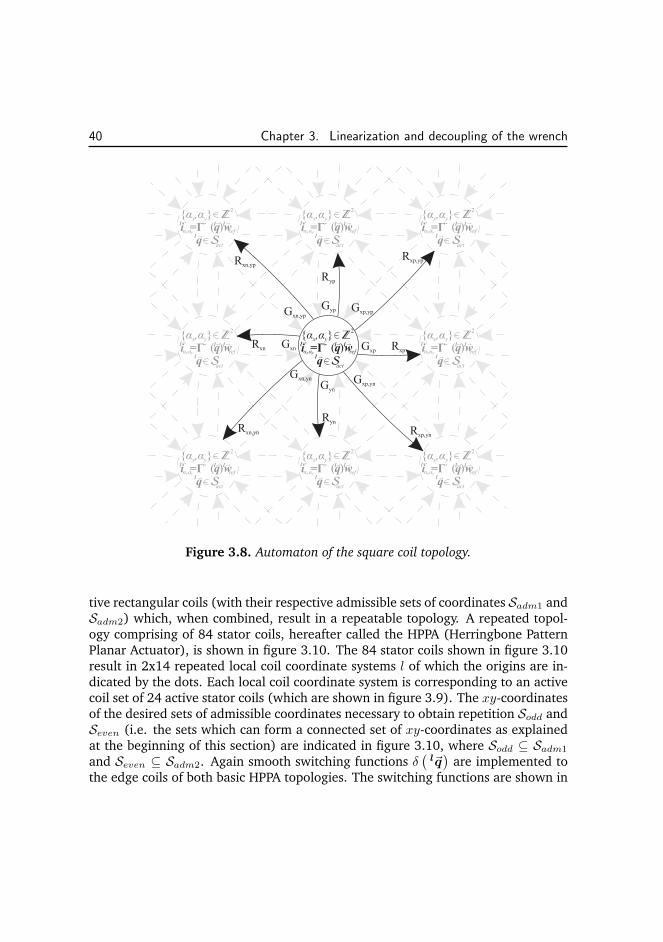
40 Chapter 3. Linearization and decoupling of the wrench
Figure 3.8. Automaton of the square coil topology.
tive rectangular coils (with their respective admissible sets of coordinates Sadm1 andSadm2) which, when combined, result in a repeatable topology. A repeated topol-ogy comprising of 84 stator coils, hereafter called the HPPA (Herringbone PatternPlanar Actuator), is shown in figure 3.10. The 84 stator coils shown in figure 3.10result in 2x14 repeated local coil coordinate systems l of which the origins are in-dicated by the dots. Each local coil coordinate system is corresponding to an activecoil set of 24 active stator coils (which are shown in figure 3.9). The xy-coordinatesof the desired sets of admissible coordinates necessary to obtain repetition Sodd andSeven (i.e. the sets which can form a connected set of xy-coordinates as explainedat the beginning of this section) are indicated in figure 3.10, where Sodd ⊆ Sadm1
and Seven ⊆ Sadm2. Again smooth switching functions δ(
l~q)
are implemented tothe edge coils of both basic HPPA topologies. The switching functions are shown in
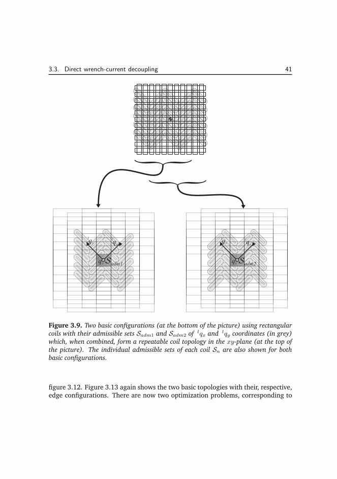
3.3. Direct wrench-current decoupling 41
Figure 3.9. Two basic configurations (at the bottom of the picture) using rectangular
coils with their admissible sets Sadm1 and Sadm2 of lqx and lqy coordinates (in grey)
which, when combined, form a repeatable coil topology in the xy-plane (at the top of
the picture). The individual admissible sets of each coil Sn are also shown for both
basic configurations.
figure 3.12. Figure 3.13 again shows the two basic topologies with their, respective,edge configurations. There are now two optimization problems, corresponding to
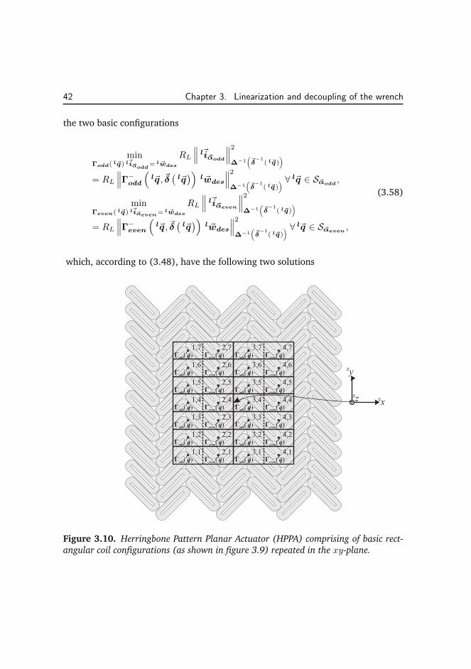
42 Chapter 3. Linearization and decoupling of the wrench
the two basic configurations
minΓodd( l~q) l~i~αodd
= l ~wdes
RL
∥
∥
∥
l~i~αodd
∥
∥
∥
2
∆−1
(
~δ−1
( l~q))
= RL
∥
∥
∥Γ−odd
(
l~q , ~δ(
l~q)
)
l ~wdes
∥
∥
∥
2
∆−1
(
~δ−1
( l~q)) ∀ l~q ∈ S~αodd
,
minΓeven( l~q) l~i~αeven= l ~wdes
RL
∥
∥
∥
l~i~αeven
∥
∥
∥
2
∆−1
(
~δ−1
( l~q))
= RL
∥
∥
∥Γ−even
(
l~q , ~δ(
l~q)
)
l ~wdes
∥
∥
∥
2
∆−1
(
~δ−1
( l~q)) ∀ l~q ∈ S~αeven
,
(3.58)
which, according to (3.48), have the following two solutions
Figure 3.10. Herringbone Pattern Planar Actuator (HPPA) comprising of basic rect-
angular coil configurations (as shown in figure 3.9) repeated in the xy-plane.
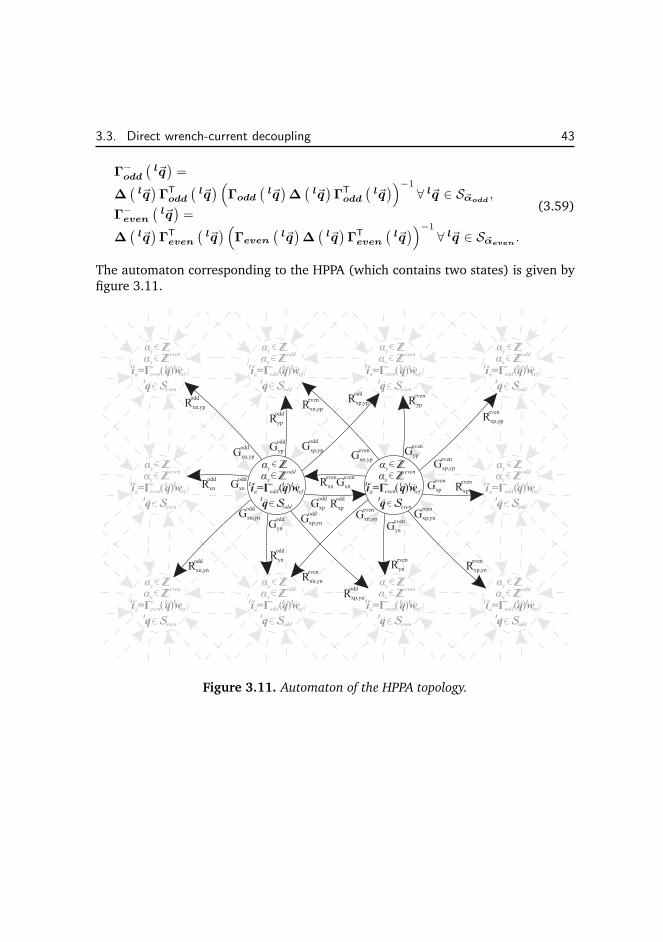
3.3. Direct wrench-current decoupling 43
Γ−odd
(
l~q)
=
∆(
l~q)
ΓT
odd
(
l~q)
(
Γodd
(
l~q)
∆(
l~q)
ΓT
odd
(
l~q)
)−1
∀ l~q ∈ S~αodd,
Γ−even
(
l~q)
=
∆(
l~q)
ΓT
even
(
l~q)
(
Γeven
(
l~q)
∆(
l~q)
ΓT
even
(
l~q)
)−1
∀ l~q ∈ S~αeven.
(3.59)
The automaton corresponding to the HPPA (which contains two states) is given byfigure 3.11.
Figure 3.11. Automaton of the HPPA topology.
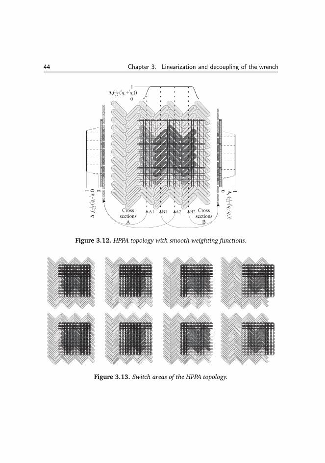
44 Chapter 3. Linearization and decoupling of the wrench
Figure 3.12. HPPA topology with smooth weighting functions.
Figure 3.13. Switch areas of the HPPA topology.
3.4. Force and torque decomposition 45
3.4 Force and torque decomposition
This section links the direct wrench-current decoupling to the traditional dq0 trans-formation described in chapter 2. The reason for this is that the decompositionwhich links the direct wrench-current decoupling to the dq0 transformation resultsin useful design criteria with respect to performance as wel as controllability.
First, the solution to minimization problem (3.47) is recalled
Γ− ( l~q
)
= ∆ΓT
(
Γ∆ΓT
)−1
∀ l~q ∈ S~α, (3.60)
where for notational simplicity the position dependency(
l~q)
has been neglected inthis section. When the wrench vector is split in the force and the torque componentsthe following equations can be defined
~w = Γl~i =
[
~F~T
]
=
[
ΓF
ΓT
]
l~i, (3.61)
where (3.60) can be rewritten as
Γ− ( l~q
)
= ∆[
ΓT
F ΓT
T
]
[
ΓF∆ΓT
F ΓF∆ΓT
T
ΓT∆ΓT
F ΓT∆ΓT
T
]−1
∀ l~q ∈ S~α. (3.62)
Using the Schur complement (see appendix A) it is possible to calculate the inverseof the partitioned matrix resulting in the following solution
l~i = Γ−T~T des +
(
I − Γ−TΓT
)
Γ−F~F des, (3.63)
with
Γ−F = ∆Γ
T
F
(
ΓF∆ΓT
F
)−1
, (3.64)
Γ−T = Φ
−Γ
T
T
(
ΓTΦ−Γ
T
T
)−1
, (3.65)
Φ− =
(
I − Γ−FΓF
)
∆, (3.66)
provided that ΓF∆ΓT
F and ΓTΦ−Γ
T
T are nonsingular. Moreover, equation (3.63)can be seen as the solution of the following two minimization problems
minΓF
l~i= l~F des
RL
∥
∥
∥
l~i∥
∥
∥
2
∆−1
= RL
∥
∥
∥Γ−F
l~F des
∥
∥
∥
2
∆−1
∀ l~q ∈ S~α , (3.67)
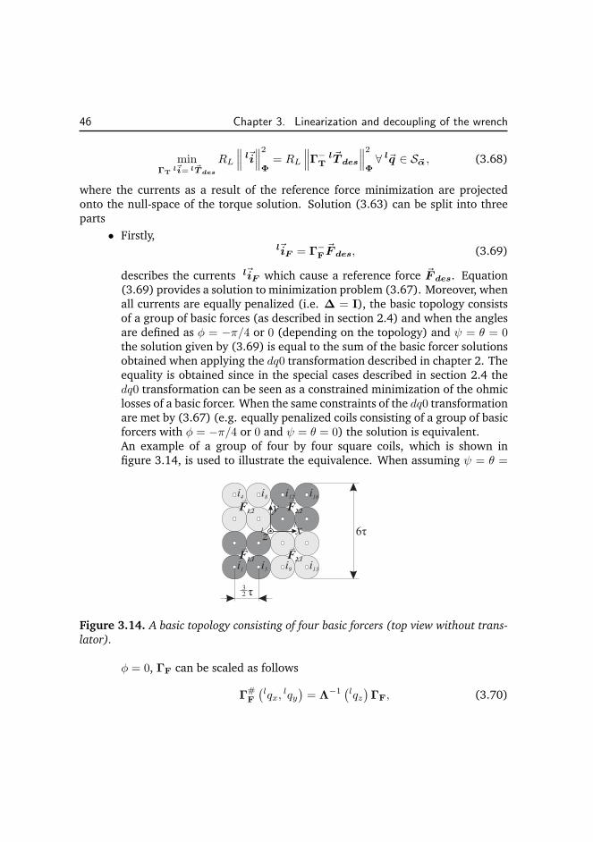
46 Chapter 3. Linearization and decoupling of the wrench
minΓT
l~i= l~T des
RL
∥
∥
∥
l~i∥
∥
∥
2
Φ= RL
∥
∥
∥Γ−T
l~T des
∥
∥
∥
2
Φ∀ l~q ∈ S~α , (3.68)
where the currents as a result of the reference force minimization are projectedonto the null-space of the torque solution. Solution (3.63) can be split into threeparts
• Firstly,l~iF = Γ
−F~F des, (3.69)
describes the currents l~iF which cause a reference force ~F des. Equation(3.69) provides a solution to minimization problem (3.67). Moreover, whenall currents are equally penalized (i.e. ∆ = I), the basic topology consistsof a group of basic forces (as described in section 2.4) and when the anglesare defined as φ = −π/4 or 0 (depending on the topology) and ψ = θ = 0the solution given by (3.69) is equal to the sum of the basic forcer solutionsobtained when applying the dq0 transformation described in chapter 2. Theequality is obtained since in the special cases described in section 2.4 thedq0 transformation can be seen as a constrained minimization of the ohmiclosses of a basic forcer. When the same constraints of the dq0 transformationare met by (3.67) (e.g. equally penalized coils consisting of a group of basicforcers with φ = −π/4 or 0 and ψ = θ = 0) the solution is equivalent.An example of a group of four by four square coils, which is shown infigure 3.14, is used to illustrate the equivalence. When assuming ψ = θ =
Figure 3.14. A basic topology consisting of four basic forcers (top view without trans-
lator).
φ = 0, ΓF can be scaled as follows
Γ#F
(
lqx,lqy)
= Λ−1(
lqz)
ΓF, (3.70)
3.4. Force and torque decomposition 47
where
Λ−1(
lqz)
=τ
π
1
λpmexp
(√2π
τlqz
)
1 0 00 1 0
0 0√
22
, (3.71)
is derived using (2.48). The solution to minimization problem (3.67) (using∆ = I) then simplifies to
Γ−F = Γ
#−F
(
lqx,lqy)
Λ−1(
lqz)
= Γ#T
F
(
lqx,lqy)
(
Γ#F
(
lqx,lqy)
Γ#T
F
(
lqx,lqy)
)−1
Λ−1(
lqz)
= Γ#T
F
(
lqx,lqy)
14 0 00 1
4 00 0 1
4
Λ−1(
lqz)
,
(3.72)
which can be explained by the fact that after normalization the matrix Γ#F
can be split into four identical orthonormal matrices (which have the prop-erty that A
−1 = AT) belonging to the four forcers. The factors 1
4 resultfrom the fact that each forcer delivers one fourth of the total force. More-over, in this case (since the forcers are all equally distributed) the systemsimplifies even further into
Γ−F = Γ
#T
F
(
lqx,lqy)
14 0 00 1
4 00 0 1
4
Λ−1(
lqz)
=
1 0 1 0 0 0 0 0 1 0 1 0 0 0 0 00 0 0 0 1 0 1 0 0 0 0 0 1 0 1 00 1 0 1 0 0 0 0 0 1 0 1 0 0 0 00 0 0 0 0 1 0 1 0 0 0 0 0 1 0 1
· efghT dqxqy0
(
lqx − cx,lqy − cy
)
0 0 − 14
14 0 00 1
4 00 0 0
Λ−1(
lqz)
,
(3.73)
where efghT dqxqy0 is derived in section 2.4 and where cx and cy are con-stant position offsets to match both coordinate systems.In case of the two basic HPPA topologies (shown in figure 3.9), the resultcan be derived in a similar way, where
Λ−1(
lqz)
=2
3
τnπ
1
λpmexp
(
π
τnlqz
)
1 0 00 1 00 0 1
, (3.74)
48 Chapter 3. Linearization and decoupling of the wrench
can be derived using (2.51). The solution to minimization problem (3.67)(using ∆ = I) then simplifies to
Γ−F = Γ
#−F
(
lqx,lqy)
Λ−1(
lqz)
= Γ#T
F
(
lqx,lqy)
(
Γ#F
(
lqx,lqy)
Γ#T
F
(
lqx,lqy)
)−1
Λ−1(
lqz)
= Γ#T
F
(
lqx,lqy)
Λ−1(
lqz)
14 0 00 1
4 00 0 1
8
.
(3.75)
which can be explained by looking at figure 3.9, where for each of the twobasic topologies there are four groups of forcers which can produce forcein the xz-plane, and four forcers which can produce force in the yz-plane,respectively, resulting in the factors 1
4 in the x- and y-directions and a factor18 in the z-direction.
• Secondly,
l~iT0F = −Γ−TΓTΓ
−F~F des , (3.76)
describes the currents l~iT0F which correct for the unwanted disturbancetorque, due to the force distribution over the translator, without produc-ing any additional force components. Ideally, these currents should be zerosince this is an unwanted effect. However, in moving-magnet planar ac-tuators this is not possible due to the variable torque arm. A good designcriteria is to keep this term as small as possible (especially with respect to apure lifting force). The 2-norm of this term is a good design criteria. The 2-norm will increase, for acceleration forces in the xy-plane, when the height(in the z direction) of the mass center point of the translator is increased.Therefore, a good design criteria is to keep the 2-norm of this terms smallwith respect to the 2-norm of the first term discussed above.
• Lastly,l~iT = Γ
−T~T des, (3.77)
describes the currents l~iT which cause a desired reference torque ~T des andno force.
Chapter 4
Design of controllable
topologies
4.1 Introduction
An interesting challenge in designing a moving-magnet planar actuator is the designof the coil layout in the stator plane while keeping the controllability in mind. Thischapter makes use of the direct wrench-current decoupling of chapter 3 as well asthe dq0 transformation derived in chapter 2 to verify the controllability of a design.Part of the design method and some of the resulting topologies have been patented[21] and published [44, 42, 19, 45].
In section 4.2, the notion of (state) controllability is introduced and appliedto the planar actuator models. In section 4.3 the theory is expanded to get a betteridea of the quality of the derived design with respect to the error sensitivity of thedecoupling algorithm. Section 4.4 applies the theory derived in sections 4.2 and 4.3to the square coil topology and the HPPA (Herringbone Pattern Planar Actuator).Section 4.5 shows how to calculate the worst case (smallest) acceleration levelswhich can be obtained in the xy-plane for a given design, decoupling and maximumcurrent specification.
4.2 State controllability conditions of a planar actuator
Throughout this chapter the notion of controllability is used. Therefore, first an in-troduction about the notion of (state) controllability (supposing that you know/canmeasure the states) is given
49
50 Chapter 4. Design of controllable topologies
Definition 4.1. State controllability. (S. Skogestad et al. [38, definition 4.1]) The
dynamical system ~x = A~x + B~u, or equivalently the pair (A,B), is said to be state
controllable if, for any initial state ~x (0) = ~x0, any time t1 > 0 and any final state ~x1,
there exists an input ~u (t) such that ~x (t1) = ~x1. Otherwise the system is said to be
uncontrollable.
The system (A,B) is state controllable if and only if the controllability matrix
C =[
B AB A2B · · ·An−1
B]
, (4.1)
has rank n (full row rank) where n is the number of states.
Definition 4.2. The planar actuators considered are a class of nonlinear systems which
can be defined as a combination of a linear system (A,B) with an additional input
mapping which is linear with respect to the current input vector l~i, but nonlinear with
respect to the position and orientation vector l~q
~x = A~x + Bl ~w, (4.2)
~x =[
l~qT l~qT]T
, (4.3)
l ~w = Γ(
l~q)
l~i, (4.4)
(4.5)
where l ~w =[
l~FT
l~TT]T
is the wrench vector consisting of the force and torque
components on the mass center point of the translator (which is considered to be a
rigid body). With the system matrices
A =
[
0 I
0 0
]
,
B =
[
0
M−1
]
,
(4.6)
where M is a diagonal matrix consisting of the mass and inertias corresponding to
each degree of freedom.
To derive a notion of controllability of this system the following definitions areintroduced.
Definition 4.3. (H. Nijmeijer et al. [32, section 3.1]) Let a smooth affine nonlinear
4.2. State controllability conditions of a planar actuator 51
control system be given by
~x = ~f (~x) +m∑
j=1
~gj (~x)uj ,
~u =[
u1 · · · um]T ∈ U ⊂ R
m,
(4.7)
where ~x are local coordinates for a smooth manifold M (the state space manifold),
and ~f ,~g1,· · · ,~gm are smooth vector fields on M. ~f is called the drift vector field, and~gj , the input vector fields.
Definition 4.4. Controllability (H. Nijmeijer et al. [32, definition 3.2]) The non-
linear system of definition 4.3 is called controllable if for any two points ~x1,~x2 in Mthere exists a finite time tf and an admissible control function ~u : [t0, tf ] → U such
that ~x (tf , t0, ~x1, ~u) = ~x2
The simplest approach to study controllability of the nonlinear system of def-inition 4.3 is to consider its linearization.
Proposition 4.5. (H. Nijmeijer et al. [32, proposition 3.3]) Consider the nonlinear
system of definition 4.3, and let ~x0 ∈ M satisfy ~f (~x0) = ~0. Furthermore, let Ucontain a neighborhood V of ~u = ~0. Suppose that the linearization of the nonlinear
system of definition 4.3 in ~x0 and ~u = ~0
~z = J~f (~x) |~x=~x0~z +
m∑
j=1
~gj (~x0) vj ,
~z ∈ Rn, ~v ∈ R
m,(4.8)
is a controllable linear system (where J~f (~x) is defined as the Jacobian of the drift
vectorfield with respect to the local coordinates ~x of the smooth manifold M). Then
for every tf > 0 and ǫ > 0 the set of points which can be reached from ~x0 in time tfusing admissible control functions u (·) : [0, tf ] → V , satisfying ‖~u (t)‖ < ǫ, contains
a neighborhood of ~x0.
This does not imply that if the linearized system is uncontrollable, the non-linear system is uncontrollable. However, in the case of a planar actuator, it is de-sirable for the system to be holonomic2, which in this case means that for every ad-missible position it should always be possible to move in all six degrees of freedom
2An example of a non-holonomic system is a car, which cannot directly move laterally resulting in anuncontrollable linearized system, although, (fortunately) it is controllable (the proof is given in [32]).
52 Chapter 4. Design of controllable topologies
directly. More formally it means that the kinematic constraints should only dependon time and the generalized coordinates, and they should not depend on their gen-eralized velocities (time derivatives of the generalized coordinates) [7]. Therefore,in the case of a the planar actuator, proposition 4.5 is a useful test method.
This can be seen when applying proposition 4.5 to the planar actuator system(definition 4.2) since
~f (~x0) = ~0, (4.9)
holds for all admissible coordinates because
~f (~x0) = A~x0 =
[
0 I
0 0
] [
l~q0
~0
]
= ~0. (4.10)
Moreover,J~f (~x) |~x=~x0
= A, (4.11)
so ~z can be substituted by ~x (in (4.8)). Now (4.8) can be simplified into
~x = A~x + BΓ(
l~q0
)
l~i, (4.12)
using definition 4.1 this results in the rank condition
rank([
BΓ(
l~q)
ABΓ(
l~q)
A2BΓ
(
l~q)
· · ·A(2#DOF−1)BΓ
(
l~q) ])
=
rank
([
0 M−1
Γ(
l~q)
M−1
Γ(
l~q)
0
])
= 2#DOF ∀ l~q ∈ S~α.(4.13)
which simplifies into the following rank condition
rank(
M−1
Γ(
l~q))
= #DOF ∀ l~q ∈ S~α. (4.14)
So, for the planar actuator to be (state) controllable, the matrix should have fullrow rank for all admissible coordinates l~q ∈ S~α. Since M
−1 is a diagonal matrixwith full rank, the condition can be simplified to
rank(
Γ(
l~q))
= #DOF ∀ l~q ∈ S~α. (4.15)
The condition derived above is the same as stating that there exists a reflexivegeneralized inverse which results in the following condition
Γ(
l~q)
Γ− ( l~q
)
= I ∀ l~q ∈ S~α, (4.16)
which can be checked using the theory of chapter 3. Moreover, when switching isnecessary to increase the stroke in the xy-plane there should exist a reflexive gener-alized inverse which also allows for smooth switching of the currents (as discussedin section 3.3.1).
4.3. Error sensitivity of weighted minimal norm inverses and solutions 53
4.3 Error sensitivity of weighted minimal norm inverses andsolutions
In the introduction of this chapter the concept of controllability is introduced. Thecondition given by (4.16) shows a test to determine whether or not a planar ac-tuator is controllable. However, this only provides a yes or no decision about thecontrollability. To compare various designs it is desirable to have a design parame-ter which is a measure of the controllability. A possibility is to look at how reliablethe diagonalization given by (4.16) will be under uncertainties. Without knowledgeof the structure of these uncertainties a qualitative indication of the decoupling canbe obtained by looking at the error sensitivity of the generalized inverse which isused in the decoupling. For this reason the condition number is introduced
Definition 4.6. With slight abuse of notation the condition number for matrix inver-
sion with respect to the induced matrix 2-norm ‖·‖ is given by the quantity
κ2
(
A−,A
)
≡{
‖A−‖ ‖A‖ , if rank (A−) = n∞, if rank (A−) < n
, (4.17)
where the induced matrix 2-norm ‖·‖ is defined as the maximum singular value of
the matrix. Matrix A− is defined as a weighted minimum norm reflexive generalized
inverse of A (see lemma 3.1). Where A is defined as an n×m matrix where n ≤ m.
The abuse of notation is caused by the fact that if ‖A−‖ 6= 1σmin(A) , where
σmax (A) and σmin (A) are the maximum and minimum singular values of A, the
condition number is defined differently compared to its usual notation which is
κ2 (A) ≡ σmax (A)
σmin (A), (4.18)
(which can be checked using singular value decomposition).
If κ2 (Γ−,Γ) is infinitely large, the condition given by (4.16) is not met, andthe system is therefore not state controllable. Moreover, the following theorem canbe used to derive an upper bound on the errors resulting from a matrix inverse.
Theorem 4.7. Let A be a matrix of size n×m with m > n and let A− be a weighted
minimum norm reflexive generalized inverse of A (see lemma 3.1). Now suppose the
real system should have been
(A + E) ~x = ~b + ~e, (4.19)
54 Chapter 4. Design of controllable topologies
instead of
A~x = ~b, (4.20)
then for small errors ‖E‖ ≪ ‖A‖κ2(A) an approximation of the upper bound on the
relative error is given by
‖~x−~x‖‖~x‖ ≈
∥
∥
∥
(
(I+A−E)−1
A−−A−)
~b+(I+A−E)−1
A−~e∥
∥
∥
‖~x‖
< κ2 (A−,A)
(
‖E‖‖A‖ + ‖~e‖
‖~b‖
)
.(4.21)
Proof. The proof is given in appendix B �
It is not useful to apply the derived theorem directly to the matrix Γ. This iscaused by the fact that the vector ~w, which is transformed to the desired current set-point by matrix Γ
−, consists of different quantities (force and torque components)having different units (N and Nm). Therefore, scaling is very important. Especiallywhen comparing various actuator designs. To obtain a valid result, a scaling needsto be introduced which ”normalizes” the wrench vector. The first step in scaling isto use the Mass/Inertia matrix M
l~q = M−1
Γ(
l~q)
l~i, (4.22)
resulting in the acceleration vector, which is here defined as the second time deriva-tive of the position vector, indicated by l~q. This still results in different units ( m
s2 andrads2 ). A possible solution is to use an effective arm in order to match the different
units. In this chapter the arms are chosen in such a way that the mechanical powerfor each degree of freedom is equally penalized
Pm = lFxyzlqxyz = lTψ
lqψ = lTθlqθ = lTφ
lqφ, (4.23)
resulting in the following effective arms
lψ =√
IψM ,
lθ =√
IθM ,
lφ =√
IφM ,
(4.24)
where M is the mass of the translator and Iψ, Iθ and Iφ are the moments of inertiaabout the mass center point of the translator in local coil coordinates l, respectively.This results in a scaling matrix
N = diag (1, 1, 1, lψ, lθ, lφ) . (4.25)
4.4. Controllable 6 DOF basic topologies 55
The normalized matrices Γ∗ and Γ
∗− then become
Γ∗ = NM
−1Γ,
Γ∗− = Γ
−MN
−1.(4.26)
An approximate upper bound on the relative error of the 2-norm of the active cur-rent vector using the normalized decoupling can now be calculated by
κ2
(
Γ∗−,Γ∗)
‖E∗‖‖Γ∗‖ +
∥
∥~e∗∥∥
∥
∥
∥
l~q∗∥∥
∥
. (4.27)
The sensitivity of the error matrix E and error vector ~e to real design variablesis also important when comparing different designs. The sensitivity of the decou-pling with respect to e.g. the position errors of the stator coil positions depends onamongst others the pole pitch τ and the amount of active coils. The relative errorof the wrench also depends on the model error due to neglected higher harmonicsof the magnetic flux density of the magnet array in combination with the stator coiltopology itself. A fair (exact) comparison between different topologies using onlythe condition number is, therefore, not possible. Moreover, when more details areavailable about the desired trajectories and the noise distribution over the degreesof freedom, it is also possible to use (setpoint dependent) scaling factors to deter-mine the best scaling ratios. Nevertheless, in the next section it is shown that thecondition number is still a useful design parameter.
4.4 Controllable 6 DOF basic topologies
In this section the design of a basic topology is discussed which allows for thetranslator to be (state) controllable in six degrees of freedom over the full range ofadmissible coordinates.
In order to do so the example of the 4 × 4 square coil topology is used, whichwas introduced in section 3.4 (the stator coils of the basic topology are again shownin figure 4.1). It is shown that when only the force components and no switchingis considered the basic topology can be expressed as four basic forcers (as definedin chapter 2). Since each of these basic forcers can produce a position independentforce vector, presumably with a different effective arm, it is safe to assume thatthe torque components can also be controlled. Moreover, since the ohmic lossesof a single basic forcer are a factor two smaller when a force in the z-direction isrequired compared to an equal force in the x- or y-directions it is safe to assumethat it will be effective with respect to producing a levitation force.
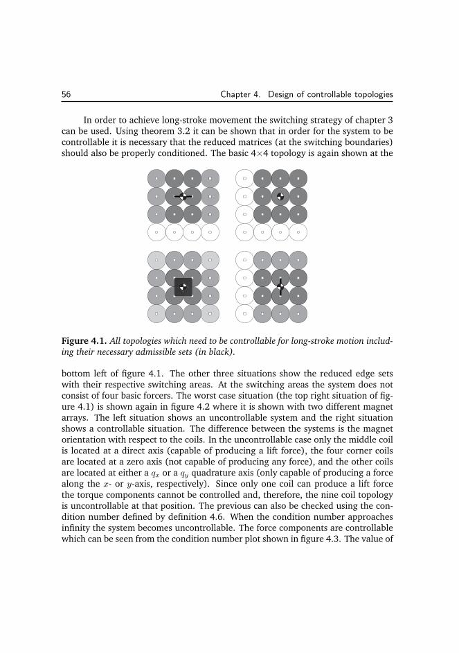
56 Chapter 4. Design of controllable topologies
In order to achieve long-stroke movement the switching strategy of chapter 3can be used. Using theorem 3.2 it can be shown that in order for the system to becontrollable it is necessary that the reduced matrices (at the switching boundaries)should also be properly conditioned. The basic 4×4 topology is again shown at the
Figure 4.1. All topologies which need to be controllable for long-stroke motion includ-
ing their necessary admissible sets (in black).
bottom left of figure 4.1. The other three situations show the reduced edge setswith their respective switching areas. At the switching areas the system does notconsist of four basic forcers. The worst case situation (the top right situation of fig-ure 4.1) is shown again in figure 4.2 where it is shown with two different magnetarrays. The left situation shows an uncontrollable system and the right situationshows a controllable situation. The difference between the systems is the magnetorientation with respect to the coils. In the uncontrollable case only the middle coilis located at a direct axis (capable of producing a lift force), the four corner coilsare located at a zero axis (not capable of producing any force), and the other coilsare located at either a qx or a qy quadrature axis (only capable of producing a forcealong the x- or y-axis, respectively). Since only one coil can produce a lift forcethe torque components cannot be controlled and, therefore, the nine coil topologyis uncontrollable at that position. The previous can also be checked using the con-dition number defined by definition 4.6. When the condition number approachesinfinity the system becomes uncontrollable. The force components are controllablewhich can be seen from the condition number plot shown in figure 4.3. The value of
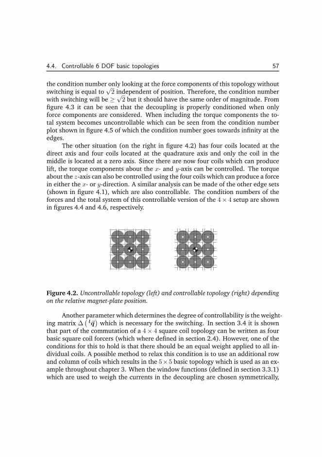
4.4. Controllable 6 DOF basic topologies 57
the condition number only looking at the force components of this topology withoutswitching is equal to
√2 independent of position. Therefore, the condition number
with switching will be ≥√
2 but it should have the same order of magnitude. Fromfigure 4.3 it can be seen that the decoupling is properly conditioned when onlyforce components are considered. When including the torque components the to-tal system becomes uncontrollable which can be seen from the condition numberplot shown in figure 4.5 of which the condition number goes towards infinity at theedges.
The other situation (on the right in figure 4.2) has four coils located at thedirect axis and four coils located at the quadrature axis and only the coil in themiddle is located at a zero axis. Since there are now four coils which can producelift, the torque components about the x- and y-axis can be controlled. The torqueabout the z-axis can also be controlled using the four coils which can produce a forcein either the x- or y-direction. A similar analysis can be made of the other edge sets(shown in figure 4.1), which are also controllable. The condition numbers of theforces and the total system of this controllable version of the 4× 4 setup are shownin figures 4.4 and 4.6, respectively.
Figure 4.2. Uncontrollable topology (left) and controllable topology (right) depending
on the relative magnet-plate position.
Another parameter which determines the degree of controllability is the weight-ing matrix ∆
(
l~q)
which is necessary for the switching. In section 3.4 it is shownthat part of the commutation of a 4 × 4 square coil topology can be written as fourbasic square coil forcers (which where defined in section 2.4). However, one of theconditions for this to hold is that there should be an equal weight applied to all in-dividual coils. A possible method to relax this condition is to use an additional rowand column of coils which results in the 5×5 basic topology which is used as an ex-ample throughout chapter 3. When the window functions (defined in section 3.3.1)which are used to weigh the currents in the decoupling are chosen symmetrically,
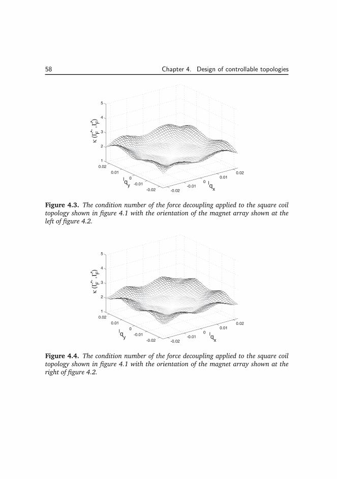
58 Chapter 4. Design of controllable topologies
Figure 4.3. The condition number of the force decoupling applied to the square coil
topology shown in figure 4.1 with the orientation of the magnet array shown at the
left of figure 4.2.
Figure 4.4. The condition number of the force decoupling applied to the square coil
topology shown in figure 4.1 with the orientation of the magnet array shown at the
right of figure 4.2.
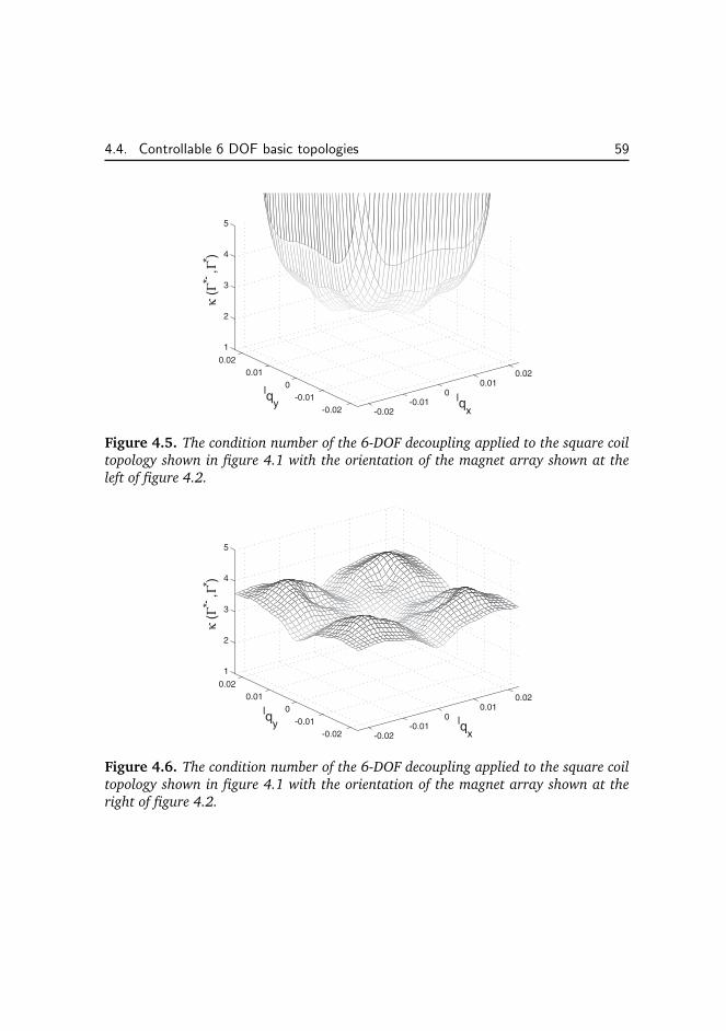
4.4. Controllable 6 DOF basic topologies 59
Figure 4.5. The condition number of the 6-DOF decoupling applied to the square coil
topology shown in figure 4.1 with the orientation of the magnet array shown at the
left of figure 4.2.
Figure 4.6. The condition number of the 6-DOF decoupling applied to the square coil
topology shown in figure 4.1 with the orientation of the magnet array shown at the
right of figure 4.2.
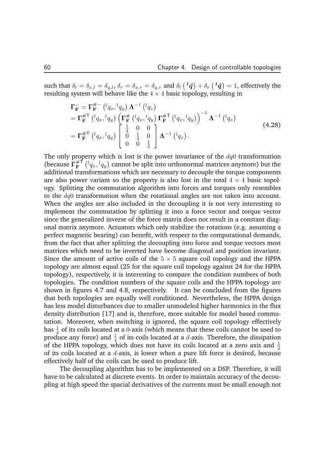
60 Chapter 4. Design of controllable topologies
such that δl = δx,l = δy,l, δr = δx,r = δy,r and δl(
l~q)
+ δr(
l~q)
= 1, effectively theresulting system will behave like the 4 × 4 basic topology, resulting in
Γ−F = Γ
#−F
(
lqx,lqy)
Λ−1(
lqz)
= Γ#T
F
(
lqx,lqy)
(
Γ#F
(
lqx,lqy)
Γ#T
F
(
lqx,lqy)
)−1
Λ−1(
lqz)
= Γ#T
F
(
lqx,lqy)
14 0 00 1
4 00 0 1
4
Λ−1(
lqz)
.
(4.28)
The only property which is lost is the power invariance of the dq0 transformation(because Γ
#T
F
(
lqx,lqy)
cannot be split into orthonormal matrices anymore) but theadditional transformations which are necessary to decouple the torque componentsare also power variant so the property is also lost in the total 4 × 4 basic topol-ogy. Splitting the commutation algorithm into forces and torques only resemblesto the dq0 transformation when the rotational angles are not taken into account.When the angles are also included in the decoupling it is not very interesting toimplement the commutation by splitting it into a force vector and torque vectorsince the generalized inverse of the force matrix does not result in a constant diag-onal matrix anymore. Actuators which only stabilize the rotations (e.g. assuming aperfect magnetic bearing) can benefit, with respect to the computational demands,from the fact that after splitting the decoupling into force and torque vectors mostmatrices which need to be inverted have become diagonal and position invariant.Since the amount of active coils of the 5 × 5 square coil topology and the HPPAtopology are almost equal (25 for the square coil topology against 24 for the HPPAtopology), respectively, it is interesting to compare the condition numbers of bothtopologies. The condition numbers of the square coils and the HPPA topology areshown in figures 4.7 and 4.8, respectively. It can be concluded from the figuresthat both topologies are equally well conditioned. Nevertheless, the HPPA designhas less model disturbances due to smaller unmodeled higher harmonics in the fluxdensity distribution [17] and is, therefore, more suitable for model based commu-tation. Moreover, when switching is ignored, the square coil topology effectivelyhas 1
4 of its coils located at a 0-axis (which means that these coils cannot be used toproduce any force) and 1
4 of its coils located at a d-axis. Therefore, the dissipationof the HPPA topology, which does not have its coils located at a zero axis and 1
2of its coils located at a d-axis, is lower when a pure lift force is desired, becauseeffectively half of the coils can be used to produce lift.
The decoupling algorithm has to be implemented on a DSP. Therefore, it willhave to be calculated at discrete events. In order to maintain accuracy of the decou-pling at high speed the spacial derivatives of the currents must be small enough not
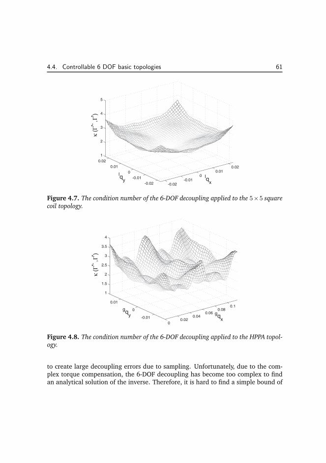
4.4. Controllable 6 DOF basic topologies 61
Figure 4.7. The condition number of the 6-DOF decoupling applied to the 5×5 square
coil topology.
Figure 4.8. The condition number of the 6-DOF decoupling applied to the HPPA topol-
ogy.
to create large decoupling errors due to sampling. Unfortunately, due to the com-plex torque compensation, the 6-DOF decoupling has become too complex to findan analytical solution of the inverse. Therefore, it is hard to find a simple bound of
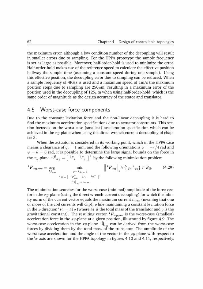
62 Chapter 4. Design of controllable topologies
the maximum error, although a low condition number of the decoupling will resultin smaller errors due to sampling. For the HPPA prototype the sample frequencyis set as large as possible. Moreover, half-order-hold is used to minimize the error.Half-order-hold makes use of the reference speed to calculate the effective positionhalfway the sample time (assuming a constant speed during one sample). Usingthis effective position, the decoupling error due to sampling can be reduced. Whena sample frequency of 4KHz is used and a maximum speed of 1m/s the maximumposition steps due to sampling are 250µm, resulting in a maximum error of theposition used in the decoupling of 125µm when using half-order-hold, which is thesame order of magnitude as the design accuracy of the stator and translator.
4.5 Worst-case force components
Due to the constant levitation force and the non-linear decoupling it is hard tofind the maximum acceleration specifications due to actuator constraints. This sec-tion focusses on the worst-case (smallest) acceleration specification which can beachieved in the xy-plane when using the direct wrench-current decoupling of chap-ter 3.
When the actuator is considered in its working point, which in the HPPA casemeans a clearance of qz = 1 mm, and the following orientations φ = −π/4 rad andψ = θ = 0 rad, it is possible to determine the large signal bounds on the force in
the xy-plane l~F xy =[
lFxlFy
]Tby the following minimization problem
l~F xy,wc = argl~F xy
minΓ− l ~w = ~i
l ~w =
[
l~FT
xy Mg l~TT
]
T
∥
∥
∥
l~i∥
∥
∥
∞= imax
∥
∥
∥
l~F xy
∥
∥
∥
2∀{
lqx,lqy}
⊂ S~α. (4.29)
The minimization searches for the worst-case (minimal) amplitude of the force vec-tor in the xy-plane (using the direct wrench-current decoupling) for which the infin-ity norm of the current vector equals the maximum current imax (meaning that oneor more of the coil currents will clip), while maintaining a constant levitation forcein the z-direction lFz = Mg (where M is the total mass of the translator and g is thegravitational constant). The resulting vector l~F xy,wc is the worst-case (smallest)acceleration force in the xy-plane at a given position, illustrated by figure 4.9. Theworst-case acceleration in the xy-plane l~qxy can be derived from the worst-caseforces by dividing them by the total mass of the translator. The amplitude of theworst-case acceleration and the angle of the vector in the xy-plane with respect tothe lx axis are shown for the HPPA topology in figures 4.10 and 4.11, respectively,
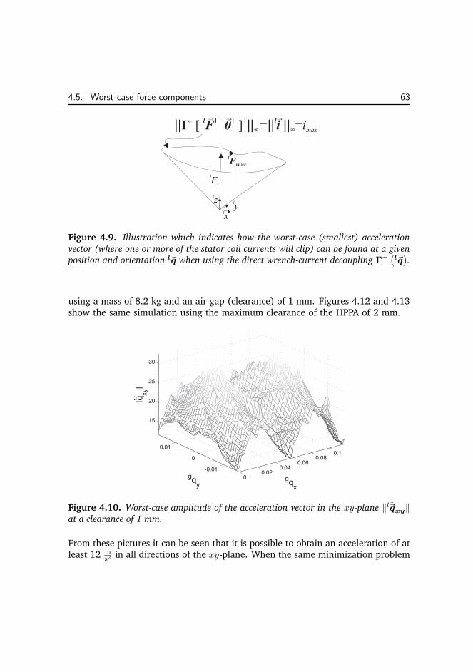
4.5. Worst-case force components 63
Figure 4.9. Illustration which indicates how the worst-case (smallest) acceleration
vector (where one or more of the stator coil currents will clip) can be found at a given
position and orientation l~q when using the direct wrench-current decoupling Γ− (l~q
)
.
using a mass of 8.2 kg and an air-gap (clearance) of 1 mm. Figures 4.12 and 4.13show the same simulation using the maximum clearance of the HPPA of 2 mm.
Figure 4.10. Worst-case amplitude of the acceleration vector in the xy-plane ‖l~qxy‖at a clearance of 1 mm.
From these pictures it can be seen that it is possible to obtain an acceleration of atleast 12 m
s2 in all directions of the xy-plane. When the same minimization problem
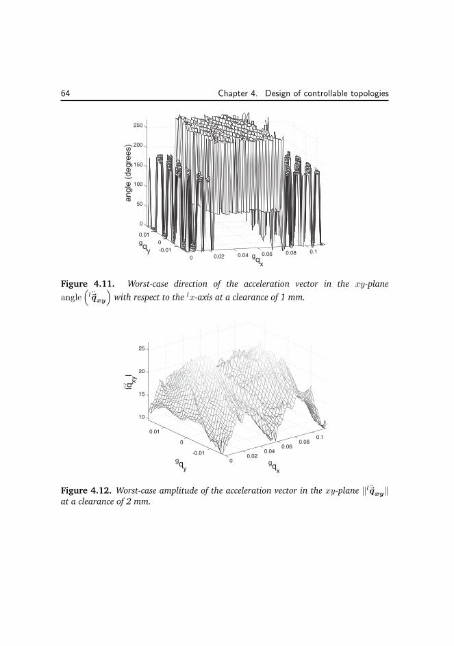
64 Chapter 4. Design of controllable topologies
Figure 4.11. Worst-case direction of the acceleration vector in the xy-plane
angle(
l~qxy
)
with respect to the lx-axis at a clearance of 1 mm.
Figure 4.12. Worst-case amplitude of the acceleration vector in the xy-plane ‖l~qxy‖at a clearance of 2 mm.
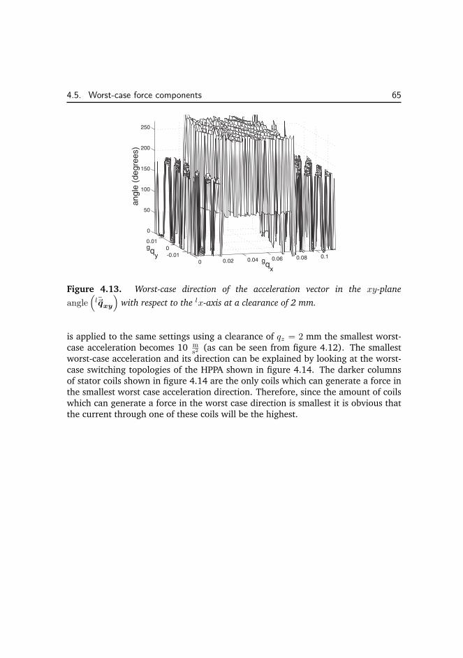
4.5. Worst-case force components 65
Figure 4.13. Worst-case direction of the acceleration vector in the xy-plane
angle(
l~qxy
)
with respect to the lx-axis at a clearance of 2 mm.
is applied to the same settings using a clearance of qz = 2 mm the smallest worst-case acceleration becomes 10 m
s2 (as can be seen from figure 4.12). The smallestworst-case acceleration and its direction can be explained by looking at the worst-case switching topologies of the HPPA shown in figure 4.14. The darker columnsof stator coils shown in figure 4.14 are the only coils which can generate a force inthe smallest worst case acceleration direction. Therefore, since the amount of coilswhich can generate a force in the worst case direction is smallest it is obvious thatthe current through one of these coils will be the highest.
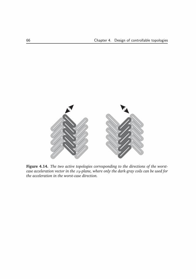
66 Chapter 4. Design of controllable topologies
Figure 4.14. The two active topologies corresponding to the directions of the worst-
case acceleration vector in the xy-plane, where only the dark-gray coils can be used for
the acceleration in the worst-case direction.
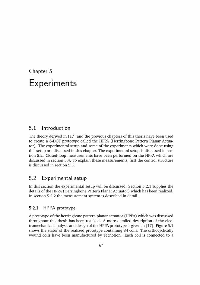
Chapter 5
Experiments
5.1 Introduction
The theory derived in [17] and the previous chapters of this thesis have been usedto create a 6-DOF prototype called the HPPA (Herringbone Pattern Planar Actua-tor). The experimental setup and some of the experiments which were done usingthis setup are discussed in this chapter. The experimental setup is discussed in sec-tion 5.2. Closed-loop measurements have been performed on the HPPA which arediscussed in section 5.4. To explain these measurements, first the control structureis discussed in section 5.3.
5.2 Experimental setup
In this section the experimental setup will be discussed. Section 5.2.1 supplies thedetails of the HPPA (Herringbone Pattern Planar Actuator) which has been realized.In section 5.2.2 the measurement system is described in detail.
5.2.1 HPPA prototype
A prototype of the herringbone pattern planar actuator (HPPA) which was discussedthroughout this thesis has been realized. A more detailed description of the elec-tromechanical analysis and design of the HPPA prototype is given in [17]. Figure 5.1shows the stator of the realized prototype containing 84 coils. The orthocyclicallywound coils have been manufactured by Tecnotion. Each coil is connected to a
67
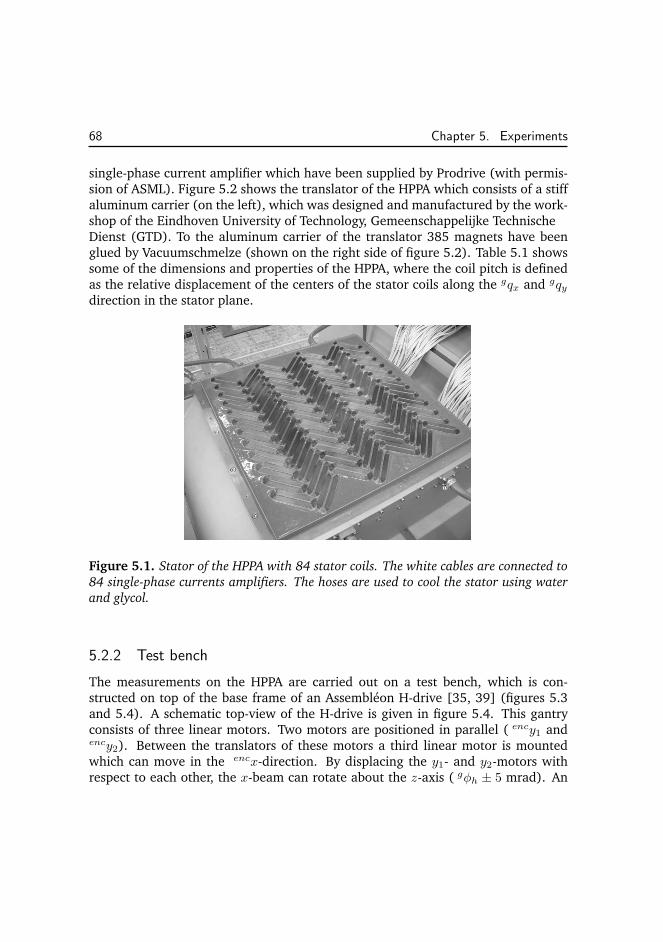
68 Chapter 5. Experiments
single-phase current amplifier which have been supplied by Prodrive (with permis-sion of ASML). Figure 5.2 shows the translator of the HPPA which consists of a stiffaluminum carrier (on the left), which was designed and manufactured by the work-shop of the Eindhoven University of Technology, Gemeenschappelijke TechnischeDienst (GTD). To the aluminum carrier of the translator 385 magnets have beenglued by Vacuumschmelze (shown on the right side of figure 5.2). Table 5.1 showssome of the dimensions and properties of the HPPA, where the coil pitch is definedas the relative displacement of the centers of the stator coils along the gqx and gqydirection in the stator plane.
Figure 5.1. Stator of the HPPA with 84 stator coils. The white cables are connected to
84 single-phase currents amplifiers. The hoses are used to cool the stator using water
and glycol.
5.2.2 Test bench
The measurements on the HPPA are carried out on a test bench, which is con-structed on top of the base frame of an Assembleon H-drive [35, 39] (figures 5.3and 5.4). A schematic top-view of the H-drive is given in figure 5.4. This gantryconsists of three linear motors. Two motors are positioned in parallel ( ency1 andency2). Between the translators of these motors a third linear motor is mountedwhich can move in the encx-direction. By displacing the y1- and y2-motors withrespect to each other, the x-beam can rotate about the z-axis ( gφh ± 5 mrad). An
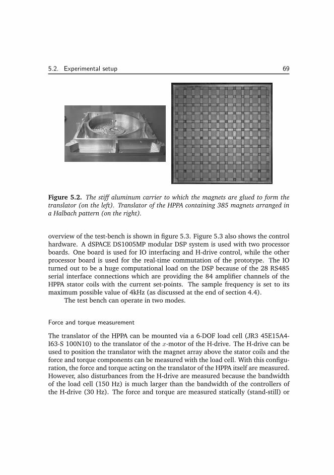
5.2. Experimental setup 69
Figure 5.2. The stiff aluminum carrier to which the magnets are glued to form the
translator (on the left). Translator of the HPPA containing 385 magnets arranged in
a Halbach pattern (on the right).
overview of the test-bench is shown in figure 5.3. Figure 5.3 also shows the controlhardware. A dSPACE DS1005MP modular DSP system is used with two processorboards. One board is used for IO interfacing and H-drive control, while the otherprocessor board is used for the real-time commutation of the prototype. The IOturned out to be a huge computational load on the DSP because of the 28 RS485serial interface connections which are providing the 84 amplifier channels of theHPPA stator coils with the current set-points. The sample frequency is set to itsmaximum possible value of 4kHz (as discussed at the end of section 4.4).
The test bench can operate in two modes.
Force and torque measurement
The translator of the HPPA can be mounted via a 6-DOF load cell (JR3 45E15A4-I63-S 100N10) to the translator of the x-motor of the H-drive. The H-drive can beused to position the translator with the magnet array above the stator coils and theforce and torque components can be measured with the load cell. With this configu-ration, the force and torque acting on the translator of the HPPA itself are measured.However, also disturbances from the H-drive are measured because the bandwidthof the load cell (150 Hz) is much larger than the bandwidth of the controllers ofthe H-drive (30 Hz). The force and torque are measured statically (stand-still) or
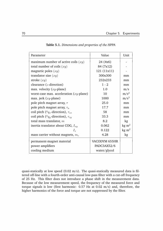
70 Chapter 5. Experiments
Table 5.1. Dimensions and properties of the HPPA
Parameter Value Unit
maximum number of active coils (xy) 24 (4x6) -
total number of coils (xy) 84 (7x12) -
magnetic poles (xy) 121 (11x11) -
translator size (xy) 300x300 mm
stroke (xy) 232x233 mm
clearance (z-direction) 1 - 2 mm
max. velocity (xy-plane) 1.0 m/s
worst-case max. acceleration (xy-plane) 10 m/s2
max. jerk (xy-plane) 1000 m/s3
pole pitch magnet array, τ 25.0 mm
pole pitch magnet array, τn 17.7 mm
coil pitch (gqx-direction), τcx 58 mm
coil pitch (gqy-direction), τcy 33.3 mm
total mass translator, m 8.2 kg
inertia translator about COG, Ixy 0.062 kg m2
Iz 0.122 kg m2
mass carrier without magnets, mc 4.28 kg
permanent-magnet material VACODYM 655HR
power amplifiers PADC3AX52/6
cooling medium water/glycol
quasi-statically at low speed (0.02 m/s). The quasi-statically measured data is fil-tered off-line with a fourth-order anti-causal low-pass filter with a cut-off frequencyof 25 Hz. This filter does not introduce a phase shift in the measurement data.Because of the low measurement speed, the frequency of the measured force andtorque signals is low (first harmonic: 0.57 Hz at 0.02 m/s) and, therefore, thehigher harmonics of the force and torque are not suppressed by the filter.
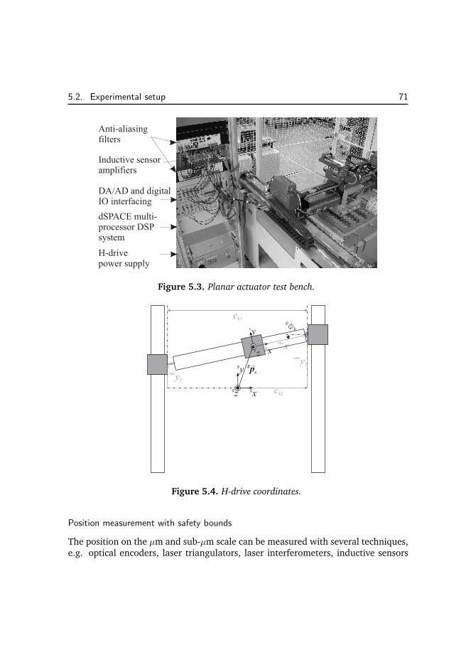
5.2. Experimental setup 71
Figure 5.3. Planar actuator test bench.
Figure 5.4. H-drive coordinates.
Position measurement with safety bounds
The position on the µm and sub-µm scale can be measured with several techniques,e.g. optical encoders, laser triangulators, laser interferometers, inductive sensors
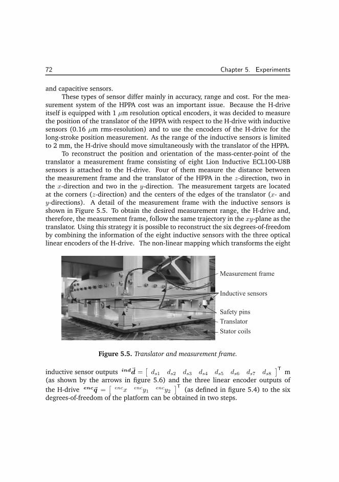
72 Chapter 5. Experiments
and capacitive sensors.These types of sensor differ mainly in accuracy, range and cost. For the mea-
surement system of the HPPA cost was an important issue. Because the H-driveitself is equipped with 1 µm resolution optical encoders, it was decided to measurethe position of the translator of the HPPA with respect to the H-drive with inductivesensors (0.16 µm rms-resolution) and to use the encoders of the H-drive for thelong-stroke position measurement. As the range of the inductive sensors is limitedto 2 mm, the H-drive should move simultaneously with the translator of the HPPA.
To reconstruct the position and orientation of the mass-center-point of thetranslator a measurement frame consisting of eight Lion Inductive ECL100-U8Bsensors is attached to the H-drive. Four of them measure the distance betweenthe measurement frame and the translator of the HPPA in the z-direction, two inthe x-direction and two in the y-direction. The measurement targets are locatedat the corners (z-direction) and the centers of the edges of the translator (x- andy-directions). A detail of the measurement frame with the inductive sensors isshown in Figure 5.5. To obtain the desired measurement range, the H-drive and,therefore, the measurement frame, follow the same trajectory in the xy-plane as thetranslator. Using this strategy it is possible to reconstruct the six degrees-of-freedomby combining the information of the eight inductive sensors with the three opticallinear encoders of the H-drive. The non-linear mapping which transforms the eight
Figure 5.5. Translator and measurement frame.
inductive sensor outputs ind~d =[
ds1 ds2 ds3 ds4 ds5 ds6 ds7 ds8]T
m(as shown by the arrows in figure 5.6) and the three linear encoder outputs of
the H-drive enc~q =[
encx ency1ency2
]T(as defined in figure 5.4) to the six
degrees-of-freedom of the platform can be obtained in two steps.
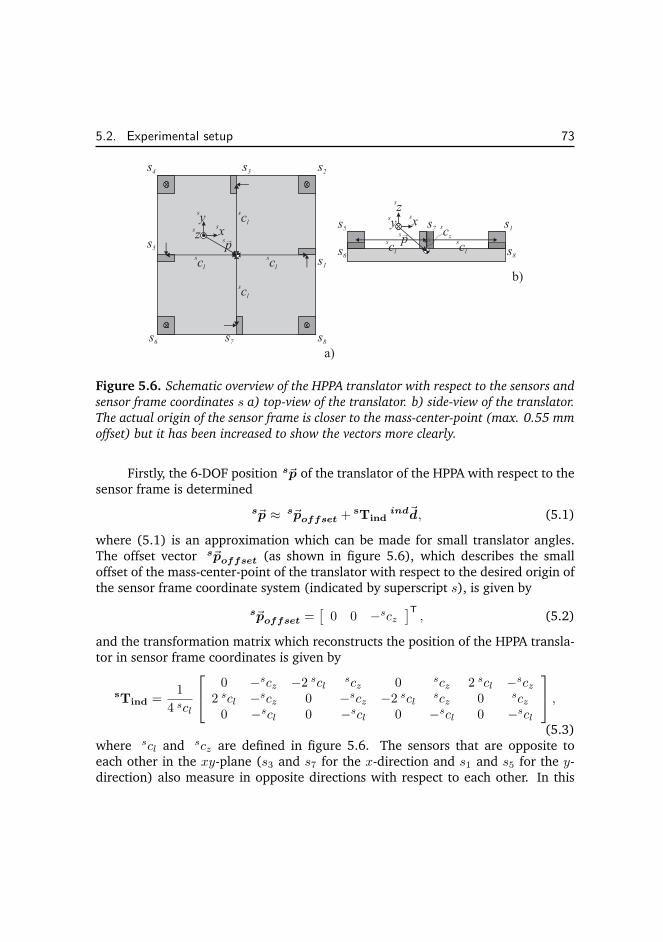
5.2. Experimental setup 73
Figure 5.6. Schematic overview of the HPPA translator with respect to the sensors and
sensor frame coordinates s a) top-view of the translator. b) side-view of the translator.
The actual origin of the sensor frame is closer to the mass-center-point (max. 0.55 mm
offset) but it has been increased to show the vectors more clearly.
Firstly, the 6-DOF position s~p of the translator of the HPPA with respect to thesensor frame is determined
s~p ≈ s~poffset + sTind
ind~d, (5.1)
where (5.1) is an approximation which can be made for small translator angles.The offset vector s~poffset (as shown in figure 5.6), which describes the smalloffset of the mass-center-point of the translator with respect to the desired origin ofthe sensor frame coordinate system (indicated by superscript s), is given by
s~poffset =[
0 0 −scz]T, (5.2)
and the transformation matrix which reconstructs the position of the HPPA transla-tor in sensor frame coordinates is given by
sTind =
1
4 scl
0 −scz −2 sclscz 0 scz 2 scl −scz
2 scl −scz 0 −scz −2 sclscz 0 scz
0 −scl 0 −scl 0 −scl 0 −scl
,
(5.3)where scl and scz are defined in figure 5.6. The sensors that are opposite toeach other in the xy-plane (s3 and s7 for the x-direction and s1 and s5 for the y-direction) also measure in opposite directions with respect to each other. In this
74 Chapter 5. Experiments
way the common noise that is picked up by the sensors is removed in the x- andy-directions because the difference of both sensor pairs is used to reconstruct the x-and y-positions (which can also be seen from the signs in the matrix s
Tind (5.3)).Moreover, this sensor placement allows for the measurement surfaces to be placedin such a way that their mass distribution does not affect the mass-center-pointof the translator in the xy-plane (it remains in the center of the translator in thexy-plane). Unfortunately, the same sensor layout cannot be used for the z-directionbecause this axis can only be measured contactless in one direction using this setup.However, there are four sensors to reconstruct this direction.
The first-order Taylor expansion of the Euler angles of the translator about itsworking point with respect to the sensor frame is used. This results in the followingapproximation of the translator angles (where sψ, sθ and sφ are the rotations aboutthe sx-, sy- and sz-axis, respectively)
sψsθsφ
≈ 1
4 scl
0 −1 0 −1 0 1 0 10 1 0 −1 0 −1 0 11 0 1 0 1 0 1 0
ind~d. (5.4)
The maximum angles of the translator about the x- and y-axes are small due tothe limited levitation height and the maximum angle about the z-axis is also keptsmall because of the limited sensor range and because the analytical model whichis used in the decoupling algorithm does not hold for large rotations about this axis.Moreover, they are kept even smaller (maximum of 6 mrad) because of safety issues(see the end of this section). Therefore, using a first-order Taylor approximationdoes not result in large errors (maximum position errors in the micrometer rangewhen using the maximum admissible angles).
However, when calculating the second transformation which transforms thesensor frame coordinates to the global coordinates using the three linear encodersof the H-drive, the transformation is not linearized with respect to the H-drive anglebecause the rotation about the z-axis of the H-drive (gφh as defined in figure 5.4)would result in unacceptable position errors in the xy-plane when using a first-order Taylor expansion due to the large distance between the point of rotation ofthe H-drive and the center of mass of the translator of the HPPA (a distance in theorder of 0.5 m in the working point of the HPPA). Therefore, the transformationof the position of the translator with respect to the sensor frame (in sensor framecoordinates s) to the position with respect to the global coordinate system (in globalcoordinates g) is given by
g~p = g~ps ( enc~q) + gRs ( enc~q) s~p, (5.5)
5.2. Experimental setup 75
where the rotation matrix is given by
gRs =
cos (gφh) − sin (gφh) 0sin (gφh) cos (gφh) 0
0 0 1
, (5.6)
and the measurement frame position in global coordinates is given by
g~ps ( enc~q) =
ch2 − encx cos(gφh)ency1 − encx sin(gφh)
ch3
, (5.7)
where encx and ency1 (which are elements of the vector enc~q) are defined in fig-ure 5.4. The sine and cosine of gφh can be reconstructed (for −π
2 < gφh < −π2 )
by
cos (gφh) = 1√
1+(
ency1−ency2ch1
)
2,
sin (gφh) =ency1−ency2
ch1
√
1+(
ency1−ency2ch1
)
2,
(5.8)
which results in an exact solution of the translator position in global coordinateswhen all angle components are zero and an approximation for small angles whichcan be calculated using the eleven sensors. The angle components of the translatorwith respect to the global coordinates can be reconstructed as follows
gψgθgφ
=
sψsθ
sφ+ gφh
. (5.9)
Because of the position measurement system, the H-drive is always movingtogether with the translator of the planar actuator. To prevent damage caused bycontact between the stator and the translator of the HPPA due to, for example,unstable controllers or power failure, the stroke of the translator of the HPPA withrespect to the measurement frame is limited by four pins (diameter 4.9 mm) whichare captured by over-sized holes (diameter 6 mm) in the translator of the HPPA.Two of these pins are indicated in Figure 5.5. The disadvantage of these pins isthat the rotation angles of the translator of the HPPA are limited to 6 mrad and therelative translation (between the translator and the measurement frame) is limitedto 1.1 mm. Once the HPPA is in control, there is no contact between its translatorand the measurement frame.
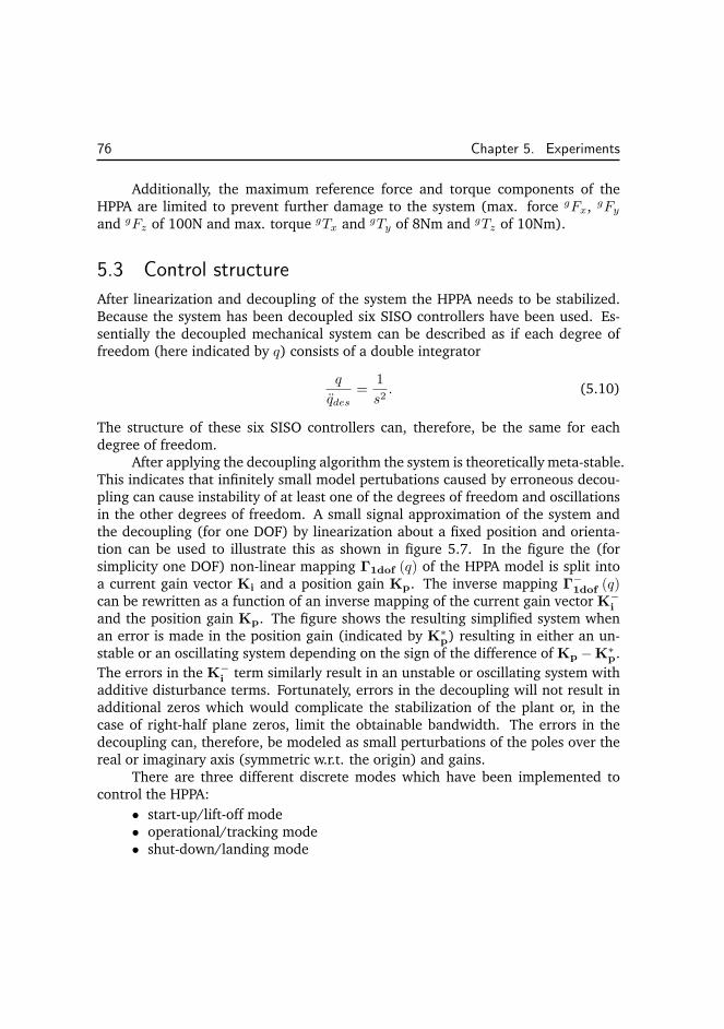
76 Chapter 5. Experiments
Additionally, the maximum reference force and torque components of theHPPA are limited to prevent further damage to the system (max. force gFx, gFyand gFz of 100N and max. torque gTx and gTy of 8Nm and gTz of 10Nm).
5.3 Control structure
After linearization and decoupling of the system the HPPA needs to be stabilized.Because the system has been decoupled six SISO controllers have been used. Es-sentially the decoupled mechanical system can be described as if each degree offreedom (here indicated by q) consists of a double integrator
q
qdes=
1
s2. (5.10)
The structure of these six SISO controllers can, therefore, be the same for eachdegree of freedom.
After applying the decoupling algorithm the system is theoretically meta-stable.This indicates that infinitely small model pertubations caused by erroneous decou-pling can cause instability of at least one of the degrees of freedom and oscillationsin the other degrees of freedom. A small signal approximation of the system andthe decoupling (for one DOF) by linearization about a fixed position and orienta-tion can be used to illustrate this as shown in figure 5.7. In the figure the (forsimplicity one DOF) non-linear mapping Γ1dof (q) of the HPPA model is split intoa current gain vector Ki and a position gain Kp. The inverse mapping Γ
−1dof (q)
can be rewritten as a function of an inverse mapping of the current gain vector K−i
and the position gain Kp. The figure shows the resulting simplified system whenan error is made in the position gain (indicated by K
∗p) resulting in either an un-
stable or an oscillating system depending on the sign of the difference of Kp −K∗p.
The errors in the K−i term similarly result in an unstable or oscillating system with
additive disturbance terms. Fortunately, errors in the decoupling will not result inadditional zeros which would complicate the stabilization of the plant or, in thecase of right-half plane zeros, limit the obtainable bandwidth. The errors in thedecoupling can, therefore, be modeled as small perturbations of the poles over thereal or imaginary axis (symmetric w.r.t. the origin) and gains.
There are three different discrete modes which have been implemented tocontrol the HPPA:
• start-up/lift-off mode• operational/tracking mode• shut-down/landing mode
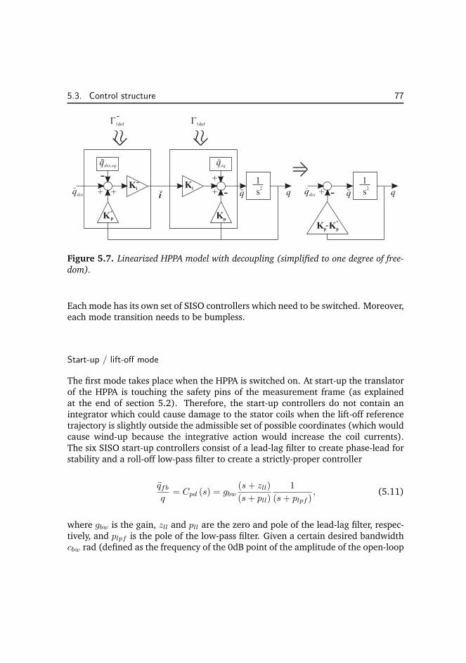
5.3. Control structure 77
Figure 5.7. Linearized HPPA model with decoupling (simplified to one degree of free-
dom).
Each mode has its own set of SISO controllers which need to be switched. Moreover,each mode transition needs to be bumpless.
Start-up / lift-off mode
The first mode takes place when the HPPA is switched on. At start-up the translatorof the HPPA is touching the safety pins of the measurement frame (as explainedat the end of section 5.2). Therefore, the start-up controllers do not contain anintegrator which could cause damage to the stator coils when the lift-off referencetrajectory is slightly outside the admissible set of possible coordinates (which wouldcause wind-up because the integrative action would increase the coil currents).The six SISO start-up controllers consist of a lead-lag filter to create phase-lead forstability and a roll-off low-pass filter to create a strictly-proper controller
qfbq
= Cpd (s) = gbw(s+ zll)
(s+ pll)
1
(s+ plpf ), (5.11)
where gbw is the gain, zll and pll are the zero and pole of the lead-lag filter, respec-tively, and plpf is the pole of the low-pass filter. Given a certain desired bandwidthcbw rad (defined as the frequency of the 0dB point of the amplitude of the open-loop
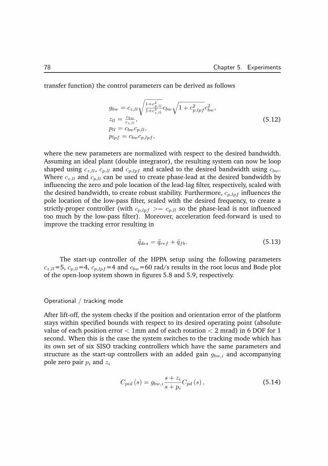
78 Chapter 5. Experiments
transfer function) the control parameters can be derived as follows
gbw = cz,ll
√
1+c2p,ll
1+c2z,ll
cbw√
1 + c2p,lpfc2bw,
zll = cbwcz,ll
,
pll = cbwcp,ll,plpf = cbwcp,lpf ,
(5.12)
where the new parameters are normalized with respect to the desired bandwidth.Assuming an ideal plant (double integrator), the resulting system can now be loopshaped using cz,ll, cp,ll and cp,lpf and scaled to the desired bandwidth using cbw.Where cz,ll and cp,ll can be used to create phase-lead at the desired bandwidth byinfluencing the zero and pole location of the lead-lag filter, respectively, scaled withthe desired bandwidth, to create robust stability. Furthermore, cp,lpf influences thepole location of the low-pass filter, scaled with the desired frequency, to create astrictly-proper controller (with cp,lpf >= cp,ll so the phase-lead is not influencedtoo much by the low-pass filter). Moreover, acceleration feed-forward is used toimprove the tracking error resulting in
qdes = qref + qfb. (5.13)
The start-up controller of the HPPA setup using the following parameterscz,ll=5, cp,ll=4, cp,lpf=4 and cbw=60 rad/s results in the root locus and Bode plotof the open-loop system shown in figures 5.8 and 5.9, respectively.
Operational / tracking mode
After lift-off, the system checks if the position and orientation error of the platformstays within specified bounds with respect to its desired operating point (absolutevalue of each position error < 1mm and of each rotation < 2 mrad) in 6 DOF for 1second. When this is the case the system switches to the tracking mode which hasits own set of six SISO tracking controllers which have the same parameters andstructure as the start-up controllers with an added gain gbw,i and accompanyingpole zero pair pi and zi
Cpid (s) = gbw,is+ zis+ pi
Cpd (s) , (5.14)
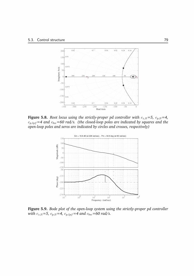
5.3. Control structure 79
Figure 5.8. Root locus using the strictly-proper pd controller with cz,ll=5, cp,ll=4,
cp,lpf=4 and cbw=60 rad/s. (the closed-loop poles are indicated by squares and the
open-loop poles and zeros are indicated by circles and crosses, respectively)
Figure 5.9. Bode plot of the open-loop system using the strictly-proper pd controller
with cz,ll=5, cp,ll=4, cp,lpf=4 and cbw=60 rad/s.
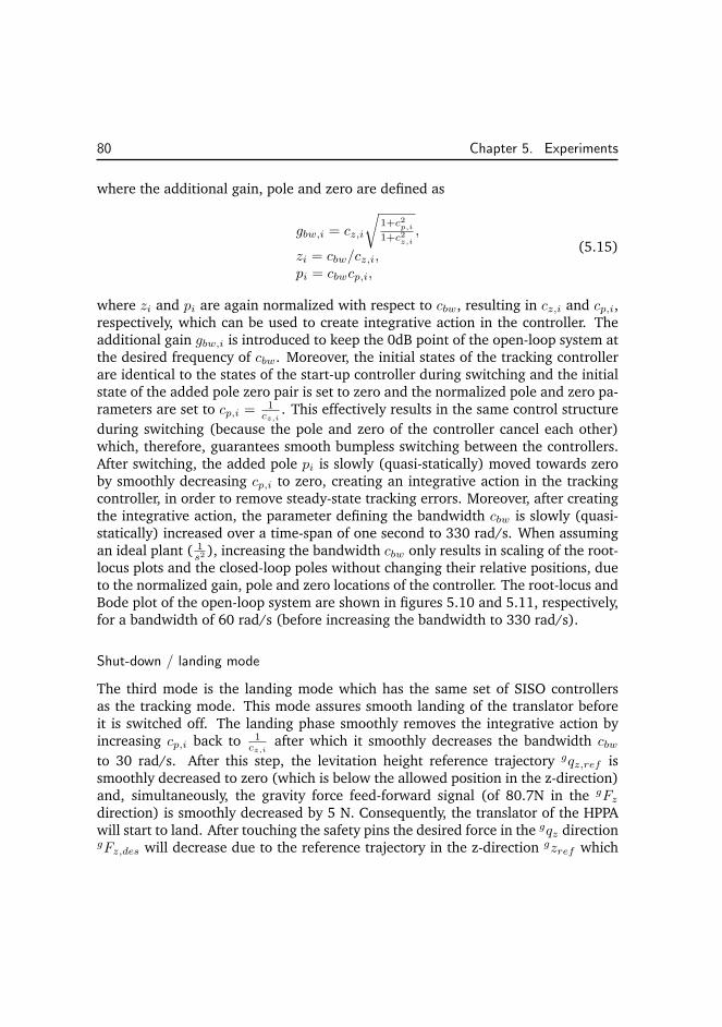
80 Chapter 5. Experiments
where the additional gain, pole and zero are defined as
gbw,i = cz,i
√
1+c2p,i1+c2z,i
,
zi = cbw/cz,i,pi = cbwcp,i,
(5.15)
where zi and pi are again normalized with respect to cbw, resulting in cz,i and cp,i,respectively, which can be used to create integrative action in the controller. Theadditional gain gbw,i is introduced to keep the 0dB point of the open-loop system atthe desired frequency of cbw. Moreover, the initial states of the tracking controllerare identical to the states of the start-up controller during switching and the initialstate of the added pole zero pair is set to zero and the normalized pole and zero pa-rameters are set to cp,i = 1
cz,i. This effectively results in the same control structure
during switching (because the pole and zero of the controller cancel each other)which, therefore, guarantees smooth bumpless switching between the controllers.After switching, the added pole pi is slowly (quasi-statically) moved towards zeroby smoothly decreasing cp,i to zero, creating an integrative action in the trackingcontroller, in order to remove steady-state tracking errors. Moreover, after creatingthe integrative action, the parameter defining the bandwidth cbw is slowly (quasi-statically) increased over a time-span of one second to 330 rad/s. When assumingan ideal plant ( 1
s2 ), increasing the bandwidth cbw only results in scaling of the root-locus plots and the closed-loop poles without changing their relative positions, dueto the normalized gain, pole and zero locations of the controller. The root-locus andBode plot of the open-loop system are shown in figures 5.10 and 5.11, respectively,for a bandwidth of 60 rad/s (before increasing the bandwidth to 330 rad/s).
Shut-down / landing mode
The third mode is the landing mode which has the same set of SISO controllersas the tracking mode. This mode assures smooth landing of the translator beforeit is switched off. The landing phase smoothly removes the integrative action byincreasing cp,i back to 1
cz,iafter which it smoothly decreases the bandwidth cbw
to 30 rad/s. After this step, the levitation height reference trajectory gqz,ref issmoothly decreased to zero (which is below the allowed position in the z-direction)and, simultaneously, the gravity force feed-forward signal (of 80.7N in the gFzdirection) is smoothly decreased by 5 N. Consequently, the translator of the HPPAwill start to land. After touching the safety pins the desired force in the gqz directiongFz,des will decrease due to the reference trajectory in the z-direction gzref which
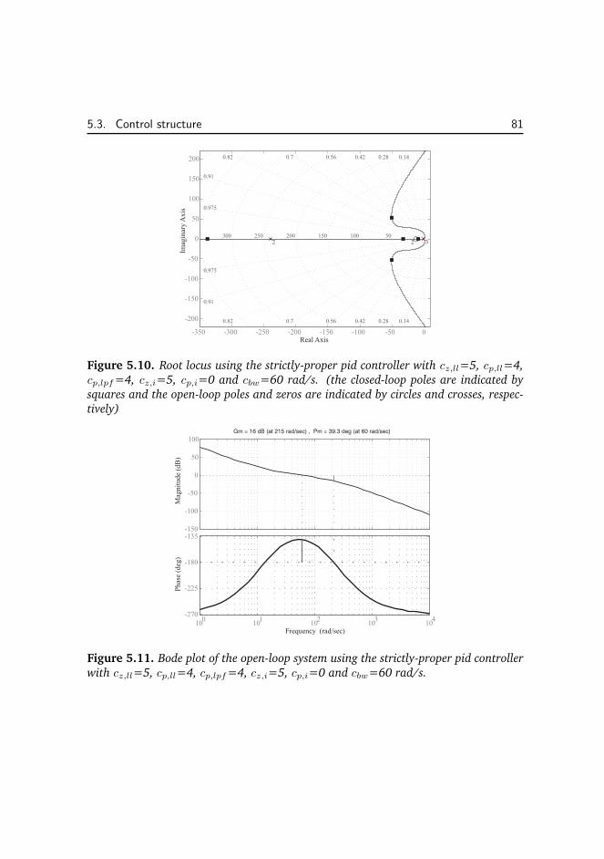
5.3. Control structure 81
Figure 5.10. Root locus using the strictly-proper pid controller with cz,ll=5, cp,ll=4,
cp,lpf=4, cz,i=5, cp,i=0 and cbw=60 rad/s. (the closed-loop poles are indicated by
squares and the open-loop poles and zeros are indicated by circles and crosses, respec-
tively)
Figure 5.11. Bode plot of the open-loop system using the strictly-proper pid controller
with cz,ll=5, cp,ll=4, cp,lpf=4, cz,i=5, cp,i=0 and cbw=60 rad/s.
82 Chapter 5. Experiments
continues to decrease. When the force output value of the controller in the z-direction gFz,des is below a threshold value of 75 N the currents are set to zero andthe system is switched off. The switch in the current set-points before switching offis dealt with by the amplifiers.
5.4 Measurement results
This section discusses the dynamic measurements which were performed on the sys-tem. Two different experiments are discussed in this section. The first experimentfocusses on closed-loop dynamical identification of the linearized and decoupledsystem using noise identification. The second experiment focusses on the trackingerrors of three specially selected trajectories.
5.4.1 Closed-loop identification
To carry out the dynamical identification of the decoupled system the system needsto be controlled first. The identification controller which was used to carry outthese experiments has the following controller parameters (which were defined insection 5.3): cz,ll=3, cp,ll=3, cp,lpf=50, cz,i=5, cp,i=0 and cbw=60 rad/s. Theresulting SISO controllers (during the tracking mode) then become
Cpid (s) = 3.18 · 107 (s+ 12) (s+ 20)
s (s+ 180) (s+ 3000). (5.16)
Using these controllers Gaussian white noise can be inserted in the loop to identifythe system using a Siglab identification device. The maximum identification strokeof the translator is limited by the safety pins because the H-drive is not excited, toprevent unwanted crosstalk of the dynamical systems. This limits the rms value ofthe noise that can be used in order to get a valid identification. The resolution ofthe measurement system is also limited because the optical linear encoders havea resolution of 1µm. This limits the maximum frequency which can be properlyidentified. The maximum frequency is limited by the expected double integrator ofthe plant because the behavior of the plant at higher frequencies needs an increas-ing amount of input power to be visible at the sensor outputs. The input poweris limited because of the thermal limits of the active stator coils (the system is al-ready dissipating because of the magnetic bearing in addition to the dissipationneeded to perform the identification). When using the controller given by (5.16)in combination with a maximum rms (gaussian) position noise of 0.2mm the max-imum frequency which can be properly identified (here defined as the frequency
5.4. Measurement results 83
for which the predicted closed-loop frequency response multiplied by the rms valueof the maximum noise reaches the quantization levels of the position encoders) ispredicted at approximately 0.2kHz. The same controller is used to identify the ro-tation where the maximum rms orientation noise is limited to 0.7mrad (which isagain limited due to the safety pins). The position noise is shaped by the controlsensitivity which results in an integrative action for very low frequencies which re-moves DC errors. Moreover, it reduces the amplitudes for the low frequencies whichare of less interest (and which would cause the translator to hit its safety margins)and it boosts the higher frequencies which are of interest (the desired cross-overfrequencies). The frequency response of the sensitivity
S (jω) = (I + P (jω)C (jω))−1, (5.17)
of the total system with controller is identified by correlating the inserted positionnoise which is inserted in the loop with the measured position and orientation er-rors. The frequency response of the plant can now be reconstructed as follows
P (jω) =(
S−1 (jω) − I
)
C−1 (jω) , (5.18)
where S (jω) is a matrix constructed out of all thirty six frequency responses ofthe system and where C (jω) is a diagonal matrix containing the six SISO trackingcontrollers for each degree of freedom. Furthermore, the plant P (jω) can be scaledusing the normalization matrix N which is defined in section 4.3 resulting in
P∗ (jω) = NP (jω)N−1, (5.19)
which now has the same units for each degree-of-freedom allowing for comparisonof the cross-terms of P
∗ (jω) with the diagonal terms.Point d shown in figure 5.12 shows the point in the xy-plane where the iden-
tification is performed. The levitation setpoint during identification has been set to1.2mm and the rotation setpoints (with respect to the general coordinate system g)have been set to zero. Figures 5.13-5.18 show the Bode plots of the diagonal termsof the transfer functions of the normalized plant and the approximate amplitudes ofthe cross-terms of the same input to the other outputs. The problem with identifyingthe cross-terms is that for higher frequencies it is not possible to insert enough noisepower to identify them properly (below position sensor resolution). The coherenceof the cross-terms of the identified sensitivity (where averaging of four independentnoise measurements is used) for the frequency components which can be excitedis very low (below 0.5). Only in the frequency band between approximately 10Hzand 20Hz the coherence is above 0.7 for the cross-terms which are above the noise
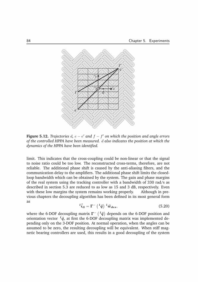
84 Chapter 5. Experiments
Figure 5.12. Trajectories d, e− e′ and f − f ′ on which the position and angle errors
of the controlled HPPA have been measured. d also indicates the position at which the
dynamics of the HPPA have been identified.
limit. This indicates that the cross-coupling could be non-linear or that the signalto noise ratio could be too low. The reconstructed cross-terms, therefore, are notreliable. The additional phase shift is caused by the anti-aliasing filters, and thecommunication delay to the amplifiers. The additional phase shift limits the closed-loop bandwidth which can be obtained by the system. The gain and phase marginsof the real system using the tracking controller with a bandwidth of 330 rad/s asdescribed in section 5.3 are reduced to as low as 15 and 3 dB, respectively. Evenwith these low margins the system remains working properly. Although in pre-vious chapters the decoupling algorithm has been defined in its most general formas
l~i~α = Γ− ( l~q
)
l ~wdes, (5.20)
where the 6-DOF decoupling matrix Γ− ( l~q
)
depends on the 6-DOF position andorientation vector l~q , at first the 6-DOF decoupling matrix was implemented de-pending only on the 3-DOF position. At normal operation, when the angles can beassumed to be zero, the resulting decoupling will be equivalent. When stiff mag-netic bearing controllers are used, this results in a good decoupling of the system
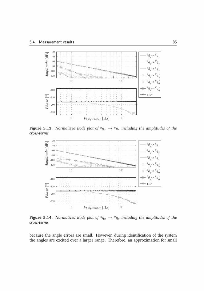
5.4. Measurement results 85
Figure 5.13. Normalized Bode plot of g qx → gqx including the amplitudes of the
cross-terms.
Figure 5.14. Normalized Bode plot of g qy → gqy including the amplitudes of the
cross-terms.
because the angle errors are small. However, during identification of the systemthe angles are excited over a larger range. Therefore, an approximation for small
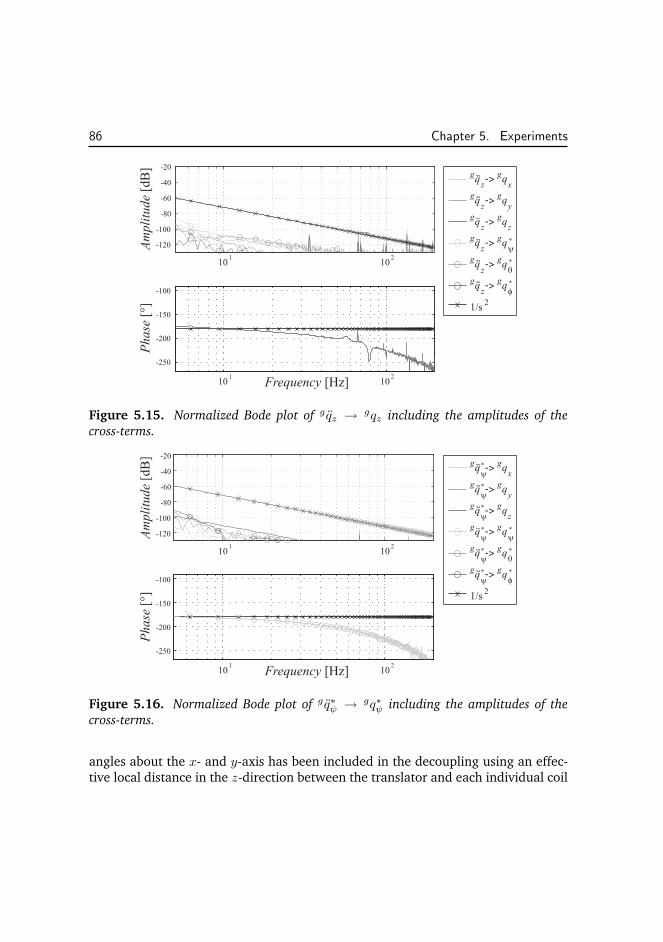
86 Chapter 5. Experiments
Figure 5.15. Normalized Bode plot of g qz → gqz including the amplitudes of the
cross-terms.
Figure 5.16. Normalized Bode plot of g q∗ψ → gq∗ψ including the amplitudes of the
cross-terms.
angles about the x- and y-axis has been included in the decoupling using an effec-tive local distance in the z-direction between the translator and each individual coil
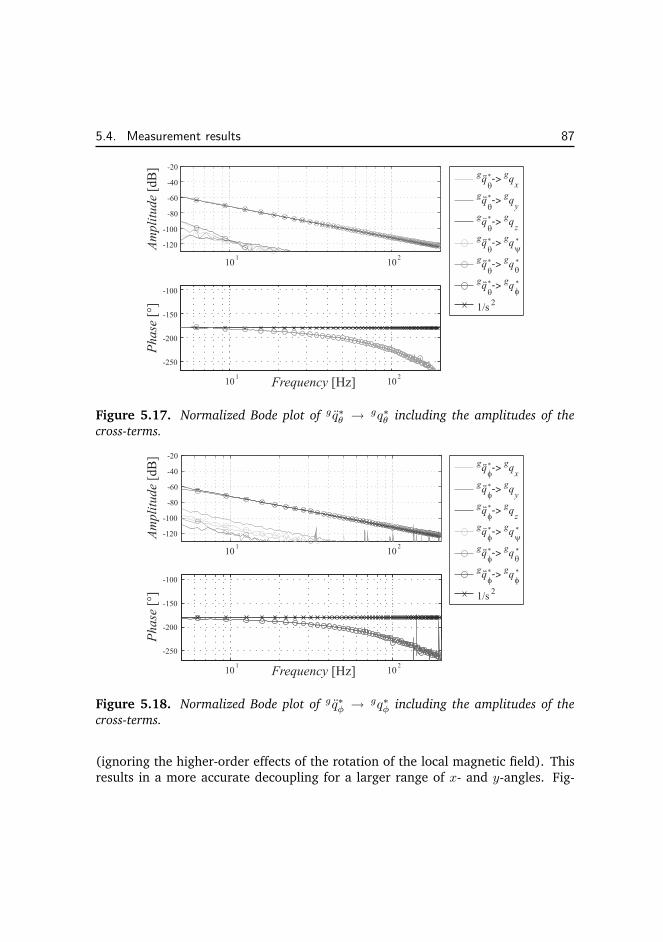
5.4. Measurement results 87
Figure 5.17. Normalized Bode plot of g q∗θ → gq∗θ including the amplitudes of the
cross-terms.
Figure 5.18. Normalized Bode plot of g q∗φ → gq∗φ including the amplitudes of the
cross-terms.
(ignoring the higher-order effects of the rotation of the local magnetic field). Thisresults in a more accurate decoupling for a larger range of x- and y-angles. Fig-
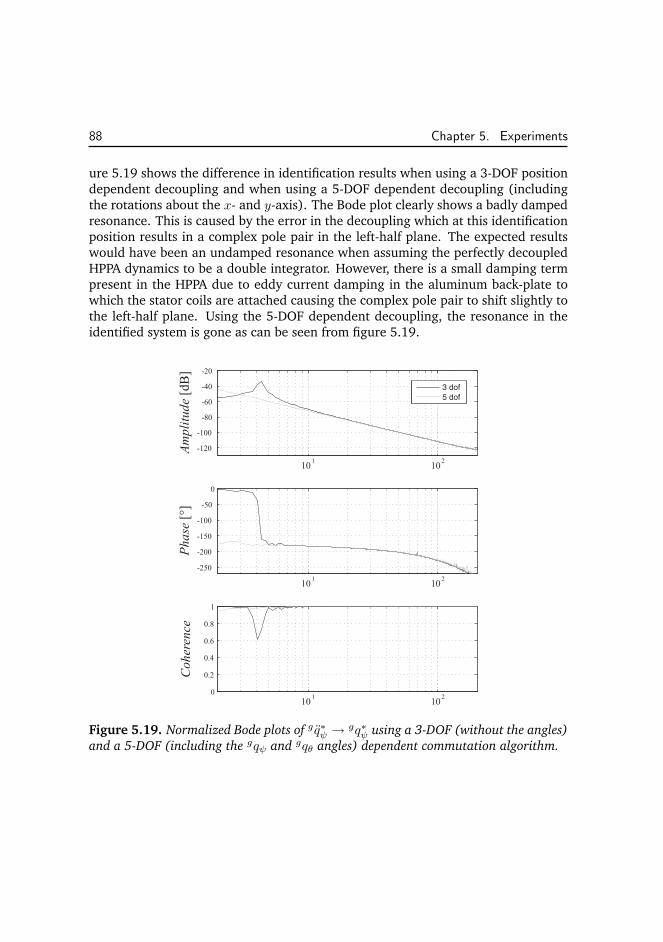
88 Chapter 5. Experiments
ure 5.19 shows the difference in identification results when using a 3-DOF positiondependent decoupling and when using a 5-DOF dependent decoupling (includingthe rotations about the x- and y-axis). The Bode plot clearly shows a badly dampedresonance. This is caused by the error in the decoupling which at this identificationposition results in a complex pole pair in the left-half plane. The expected resultswould have been an undamped resonance when assuming the perfectly decoupledHPPA dynamics to be a double integrator. However, there is a small damping termpresent in the HPPA due to eddy current damping in the aluminum back-plate towhich the stator coils are attached causing the complex pole pair to shift slightly tothe left-half plane. Using the 5-DOF dependent decoupling, the resonance in theidentified system is gone as can be seen from figure 5.19.
Figure 5.19. Normalized Bode plots of g q∗ψ → gq∗ψ using a 3-DOF (without the angles)
and a 5-DOF (including the gqψ and gqθ angles) dependent commutation algorithm.
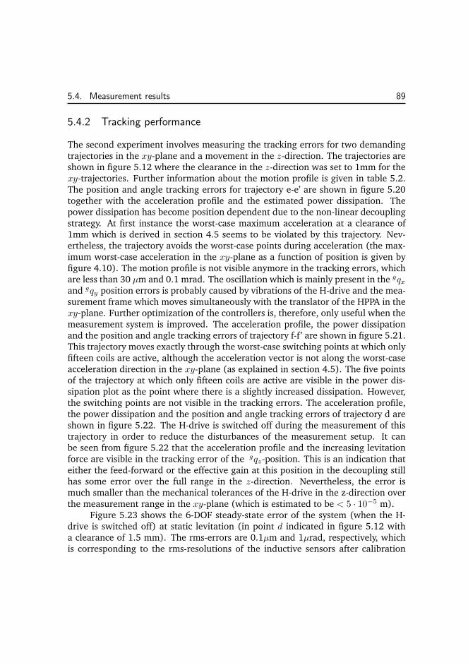
5.4. Measurement results 89
5.4.2 Tracking performance
The second experiment involves measuring the tracking errors for two demandingtrajectories in the xy-plane and a movement in the z-direction. The trajectories areshown in figure 5.12 where the clearance in the z-direction was set to 1mm for thexy-trajectories. Further information about the motion profile is given in table 5.2.The position and angle tracking errors for trajectory e-e’ are shown in figure 5.20together with the acceleration profile and the estimated power dissipation. Thepower dissipation has become position dependent due to the non-linear decouplingstrategy. At first instance the worst-case maximum acceleration at a clearance of1mm which is derived in section 4.5 seems to be violated by this trajectory. Nev-ertheless, the trajectory avoids the worst-case points during acceleration (the max-imum worst-case acceleration in the xy-plane as a function of position is given byfigure 4.10). The motion profile is not visible anymore in the tracking errors, whichare less than 30 µm and 0.1 mrad. The oscillation which is mainly present in the gqxand gqy position errors is probably caused by vibrations of the H-drive and the mea-surement frame which moves simultaneously with the translator of the HPPA in thexy-plane. Further optimization of the controllers is, therefore, only useful when themeasurement system is improved. The acceleration profile, the power dissipationand the position and angle tracking errors of trajectory f-f’ are shown in figure 5.21.This trajectory moves exactly through the worst-case switching points at which onlyfifteen coils are active, although the acceleration vector is not along the worst-caseacceleration direction in the xy-plane (as explained in section 4.5). The five pointsof the trajectory at which only fifteen coils are active are visible in the power dis-sipation plot as the point where there is a slightly increased dissipation. However,the switching points are not visible in the tracking errors. The acceleration profile,the power dissipation and the position and angle tracking errors of trajectory d areshown in figure 5.22. The H-drive is switched off during the measurement of thistrajectory in order to reduce the disturbances of the measurement setup. It canbe seen from figure 5.22 that the acceleration profile and the increasing levitationforce are visible in the tracking error of the gqz-position. This is an indication thateither the feed-forward or the effective gain at this position in the decoupling stillhas some error over the full range in the z-direction. Nevertheless, the error ismuch smaller than the mechanical tolerances of the H-drive in the z-direction overthe measurement range in the xy-plane (which is estimated to be < 5 · 10−5 m).
Figure 5.23 shows the 6-DOF steady-state error of the system (when the H-drive is switched off) at static levitation (in point d indicated in figure 5.12 witha clearance of 1.5 mm). The rms-errors are 0.1µm and 1µrad, respectively, whichis corresponding to the rms-resolutions of the inductive sensors after calibration
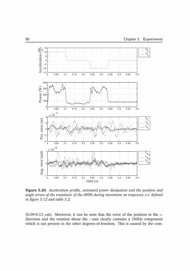
90 Chapter 5. Experiments
Figure 5.20. Acceleration profile, estimated power dissipation and the position and
angle errors of the translator of the HPPA during movement on trajectory e-e’ defined
in figure 5.12 and table 5.2.
(0.09-0.13 µm). Moreover, it can be seen that the error of the position in the z-direction and the rotation about the z-axis clearly contains a 100Hz componentwhich is not present in the other degrees-of-freedom. This is caused by the com-
5.4. Measurement results 91
Figure 5.21. Acceleration profile, estimated power dissipation and the position and
angle errors of the translator of the HPPA during movement on trajectory f-f ’ defined
in figure 5.12 and table 5.2.
mon noise of the inductive sensors, which is not canceled for these two degrees-of-freedom (which is explained in section 5.2.2).
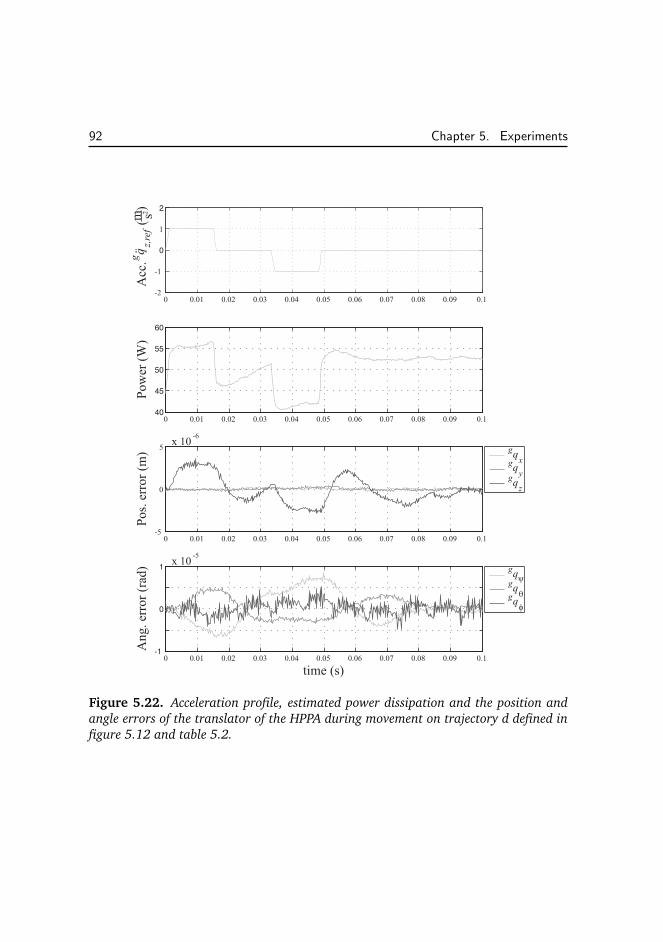
92 Chapter 5. Experiments
Figure 5.22. Acceleration profile, estimated power dissipation and the position and
angle errors of the translator of the HPPA during movement on trajectory d defined in
figure 5.12 and table 5.2.
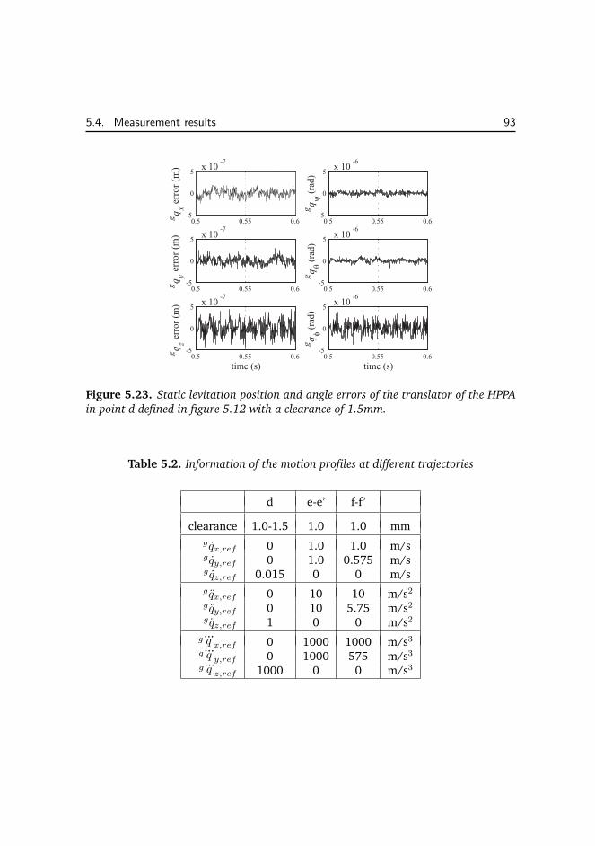
5.4. Measurement results 93
Figure 5.23. Static levitation position and angle errors of the translator of the HPPA
in point d defined in figure 5.12 with a clearance of 1.5mm.
Table 5.2. Information of the motion profiles at different trajectories
d e-e’ f-f’
clearance 1.0-1.5 1.0 1.0 mm
g qx,ref 0 1.0 1.0 m/sg qy,ref 0 1.0 0.575 m/sg qz,ref 0.015 0 0 m/s
g qx,ref 0 10 10 m/s2g qy,ref 0 10 5.75 m/s2g qz,ref 1 0 0 m/s2
g ...q x,ref 0 1000 1000 m/s3
g ...q y,ref 0 1000 575 m/s3
g ...q z,ref 1000 0 0 m/s3

94 Chapter 5. Experiments
Chapter 6
Conclusions and
recommendations
Control aspects, and the design aspects for controllability, of ironless long-strokeplanar actuators with moving magnets and integrated active magnetic bearing havebeen investigated in this thesis. The combined research in electromechanical designand control presented in [17] and this thesis has resulted in a solid fundament tothe electromagnetic analysis, model based commutation and design of this type ofactuators. Moreover, the research has resulted in a fully operational and success-fully tested prototype, the Herringbone Pattern Planar Actuator (HPPA).
6.1 Model based commutation algorithm
A novel commutation strategy, called direct wrench-current decoupling, has beenpresented in this thesis. Using the derived commutation algorithms it is possi-ble to decouple both the force as well as the torque components of an ironlessmoving-magnet planar actuator. Moreover, the commutation algorithm also allowsfor smooth switching of active coil sets without influencing the decoupling, becauseonly the coils that are underneath or near the edge of the magnet array effectivelycontribute to the magnetic bearing and propulsion of the translator. The commuta-tion algorithm is decomposed into force and torque components where one of theforce components has similarities with the traditional dq0 or Park’s transformationlinking the new theory to the traditional one.
95
96 Chapter 6. Conclusions and recommendations
6.2 Linking control to the design proces
Using the condition number of the direct wrench-current decoupling it is possible toverify whether or not a stator coil topology is state-controllable in a given positionof the translator. Moreover, additional conditions have been derived which allowfor the design/verification of controllable stator coil topologies with the capabilityof an infinite stroke in the xy-plane using smooth switching functions.
The currents resulting in a force distribution, which is optimal with respect tothe minimal ohmic losses when ignoring the disturbance torque, can be calculatedfor a given stator coil topology. Moreover, an expression of the stator coil currentscan be calculated which can be used to correct the optimal force distribution in sucha way that the disturbance torque is canceled in an optimal way with respect to theohmic losses. These currents do not contribute to the netto force on the translator.Therefore, keeping the power dissipation caused by this second term as small aspossible is an important performance criteria for the actuator.
Given an ironless planar moving-magnet actuator, using the derived commu-tation strategy, it is possible to calculate the direction and amplitude of the smallestworst-case acceleration vector in the xy-plane, over the entire set of admissible x-,y- and z-positions, which results in one or more of the stator coil currents reachingthe maximum amplifier current constraint.
6.3 Realization and test of the prototype
A prototype of an ironless moving-magnet planar actuator with integrated magneticbearing called the ”herringbone pattern planar actuator” (HPPA) has been realizedand tested successfully. The translator can be levitated at standstill with a positionerror and an angle error of < 0.5µm and < 4µrad, respectively. The tracking errorsat high-speed motion profiles, using a maximum test speed of 1.4m/s and an accel-eration of 14m/s2, are < 30µm for the position error and < 0.1mrad for the angleerror.
Currently, the measurement system is most likely to be the limiting factor inthe performance of the HPPA prototype. Parasitic effects due to the dynamic cou-pling between the measurement frame and the HPPA make it hard to separate thereal dynamics of the HPPA from the dynamics of the measurement frame. In orderto further investigate the prototype, it is advisable to remove it from the H-driveand install a measurement system which measures the position and orientation ofthe translator directly.
6.4. Outlook towards future developments 97
6.4 Outlook towards future developments
6.4.1 Full rotation about the z-axis
The derived commutation algorithm is not necessarily limited to long-stroke xy-movement. The fundamentally limited stroke in the z-direction results in a limitedrotation about the x- and y-axis because an increasing clearance between the statorcoils and the magnet array results in less force. However, extension of the actuatordesign and commutation algorithms to include full rotation about the z-axis couldincrease the functionality of planar actuators. Finding and validating controllabletopologies which allow for this increased functionality is challenging because of thevariable pole-pitch during rotation and the increased model complexity.
6.4.2 Planar actuators with non-holonomic constraints
There could be applications for which the accuracy during planar movement is notnecessarily desired over the full xy-range. Moreover, when transportation fromone section of accurate positioning to another section of accurate positioning isdesired, reduction of the number of coils can probably be obtained by allowing fornon-holonomic constraints on the system in the transportation area. Using theseconstraints only a finite set of trajectories is controllable in the transportation area.An example could be to accelerate the translator to a speed which is high enoughto reach the destination area without the need for instantaneous 6-DOF decoupling(and low power consumption) of the degrees of freedom in all positions of thetransportation area.
6.4.3 Fault tolerant planar actuator commutation
The commutation algorithm can be adapted to become fault-tolerant when it is pos-sible to detect which coils are not working properly anymore. These coils should bepenalized in the decoupling. As long as the rank of the decoupling does not dropdue to the decreased number of active coils the system will still be operational, al-though the performance will decrease slightly because the currents in the remainingcoils will increase.
6.4.4 Wireless power transfer, data communication and control
The advantage of a moving-magnet planar actuator over a moving-coil planar ac-tuator is the absence of cables. With a contactless energy supply and wireless com-
98 Chapter 6. Conclusions and recommendations
munication, a manipulator on top of the translator of the planar actuator could becontrolled while maintaining a contactless system. Information of the sensors canbe communicated through radio, optical or inductive links. A robust control strat-egy of the stacked drives has to be derived which can deal with the influences ofwireless interfacing in an optimal way (e.g. communication delays and data-loss).
A project has already been started to investigate and demonstrate a planaractuator with a manipulator, which has a contactless energy supply and wirelessdata communication and control [20, 14].
6.4.5 Multiple translators above one stator
The realized planar actuator consists of one stator and one translator. With anappropriate measurement system, also multiple translators can be levitated above asingle stator. Because cables to the translator are not required, there is also no riskof cables being tangled.
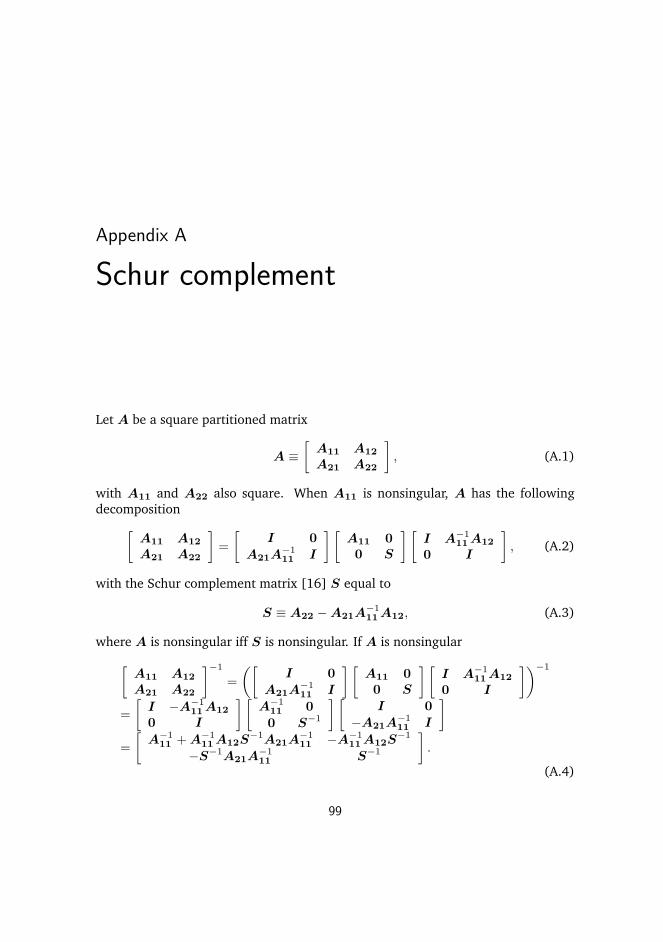
Appendix A
Schur complement
Let A be a square partitioned matrix
A ≡[
A11 A12
A21 A22
]
, (A.1)
with A11 and A22 also square. When A11 is nonsingular, A has the followingdecomposition
[
A11 A12
A21 A22
]
=
[
I 0
A21A−111 I
] [
A11 0
0 S
] [
I A−111 A12
0 I
]
, (A.2)
with the Schur complement matrix [16] S equal to
S ≡ A22 − A21A−111 A12, (A.3)
where A is nonsingular iff S is nonsingular. If A is nonsingular
[
A11 A12
A21 A22
]−1
=
([
I 0
A21A−111 I
] [
A11 0
0 S
] [
I A−111 A12
0 I
])−1
=
[
I −A−111 A12
0 I
] [
A−111 0
0 S−1
] [
I 0
−A21A−111 I
]
=
[
A−111 + A−1
11 A12S−1A21A−111 −A−1
11 A12S−1
−S−1A21A−111 S−1
]
.
(A.4)
99

100 Appendix A. Schur complement
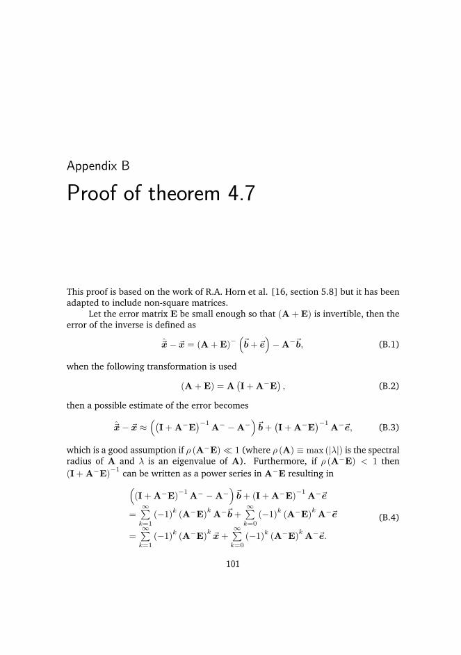
Appendix B
Proof of theorem 4.7
This proof is based on the work of R.A. Horn et al. [16, section 5.8] but it has beenadapted to include non-square matrices.
Let the error matrix E be small enough so that (A + E) is invertible, then theerror of the inverse is defined as
~x − ~x = (A + E)−(
~b + ~e)
− A−~b, (B.1)
when the following transformation is used
(A + E) = A(
I + A−E)
, (B.2)
then a possible estimate of the error becomes
~x − ~x ≈(
(
I + A−E)−1
A− − A
−)
~b +(
I + A−E)−1
A−~e, (B.3)
which is a good assumption if ρ (A−E) ≪ 1 (where ρ (A) ≡ max (|λ|) is the spectral
radius of A and λ is an eigenvalue of A). Furthermore, if ρ (A−E) < 1 then
(I + A−E)
−1can be written as a power series in A
−E resulting in
(
(I + A−E)
−1A
− − A−)
~b + (I + A−E)
−1A
−~e
=∞∑
k=1
(−1)k(A−
E)kA
−~b +∞∑
k=0
(−1)k(A−
E)kA
−~e
=∞∑
k=1
(−1)k(A−
E)k~x +
∞∑
k=0
(−1)k(A−
E)kA
−~e.
(B.4)
101
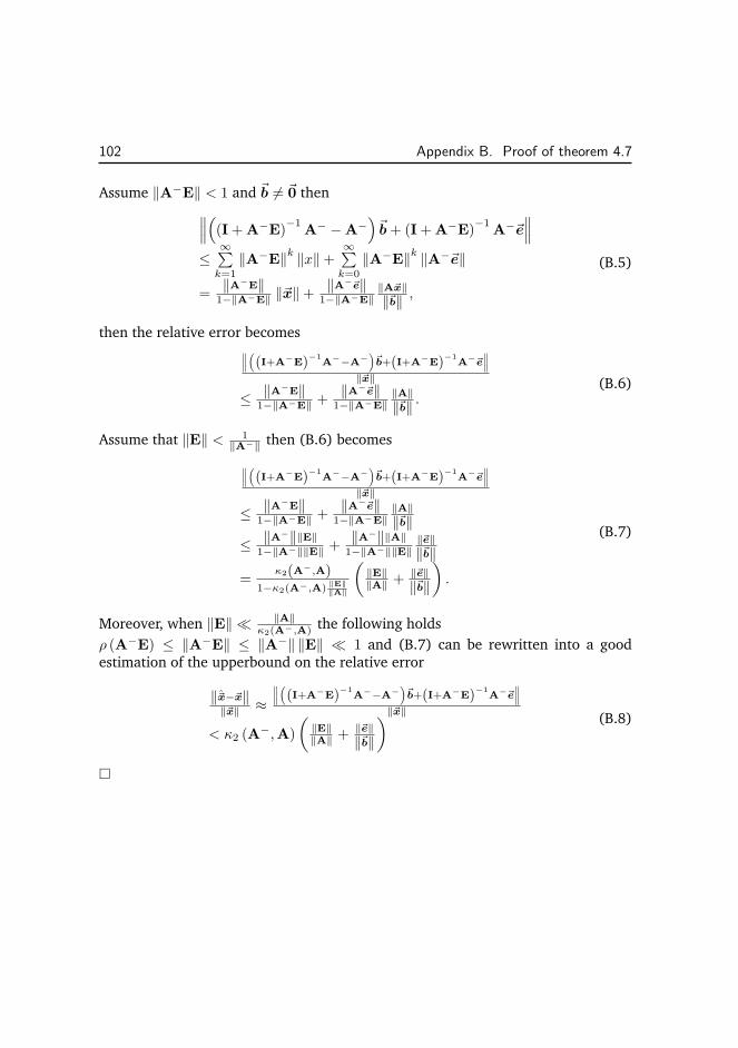
102 Appendix B. Proof of theorem 4.7
Assume ‖A−E‖ < 1 and ~b 6= ~0 then
∥
∥
∥
(
(I + A−E)
−1A
− − A−)
~b + (I + A−E)
−1A
−~e∥
∥
∥
≤∞∑
k=1
‖A−E‖k ‖x‖ +
∞∑
k=0
‖A−E‖k ‖A−~e‖
=‖A−E‖
1−‖A−E‖ ‖~x‖ +‖A−~e‖
1−‖A−E‖‖A~x‖‖~b‖ ,
(B.5)
then the relative error becomes∥
∥
∥
(
(I+A−E)−1
A−−A−)
~b+(I+A−E)−1
A−~e∥
∥
∥
‖~x‖
≤ ‖A−E‖1−‖A−E‖ +
‖A−~e‖1−‖A−E‖
‖A‖‖~b‖ .
(B.6)
Assume that ‖E‖ < 1‖A−‖ then (B.6) becomes
∥
∥
∥
(
(I+A−E)−1
A−−A−)
~b+(I+A−E)−1
A−~e∥
∥
∥
‖~x‖
≤ ‖A−E‖1−‖A−E‖ +
‖A−~e‖1−‖A−E‖
‖A‖‖~b‖
≤ ‖A−‖‖E‖1−‖A−‖‖E‖ +
‖A−‖‖A‖1−‖A−‖‖E‖
‖~e‖‖~b‖
=κ2(A−,A)
1−κ2(A−,A)‖E‖‖A‖
(
‖E‖‖A‖ + ‖~e‖
‖~b‖
)
.
(B.7)
Moreover, when ‖E‖ ≪ ‖A‖κ2(A−,A) the following holds
ρ (A−E) ≤ ‖A−
E‖ ≤ ‖A−‖ ‖E‖ ≪ 1 and (B.7) can be rewritten into a goodestimation of the upperbound on the relative error
‖~x−~x‖‖~x‖ ≈
∥
∥
∥
(
(I+A−E)−1
A−−A−)
~b+(I+A−E)−1
A−~e∥
∥
∥
‖~x‖
< κ2 (A−,A)
(
‖E‖‖A‖ + ‖~e‖
‖~b‖
) (B.8)
�

Appendix C
List of symbols
Symbol Units Quantity
~ Vector~q m,rad Coordinate vectorq quadrature axisd direct axis~i A Current vector~u V Voltage vector~F N Force vector~T Nm Torque vector~w N,Nm Wrench vector consisting of force and torque compo-
nentsT Transformation matrix≻ Positive-definite matrixc Coil coordinatesm Magnet coordinatesl Local coil coordinatesg General coordinatess Sensor coordinatesSn Admissible set of coordinates of a single coil n
Sadm Admissible set of coordinates of a basic active coilconfiguration
103
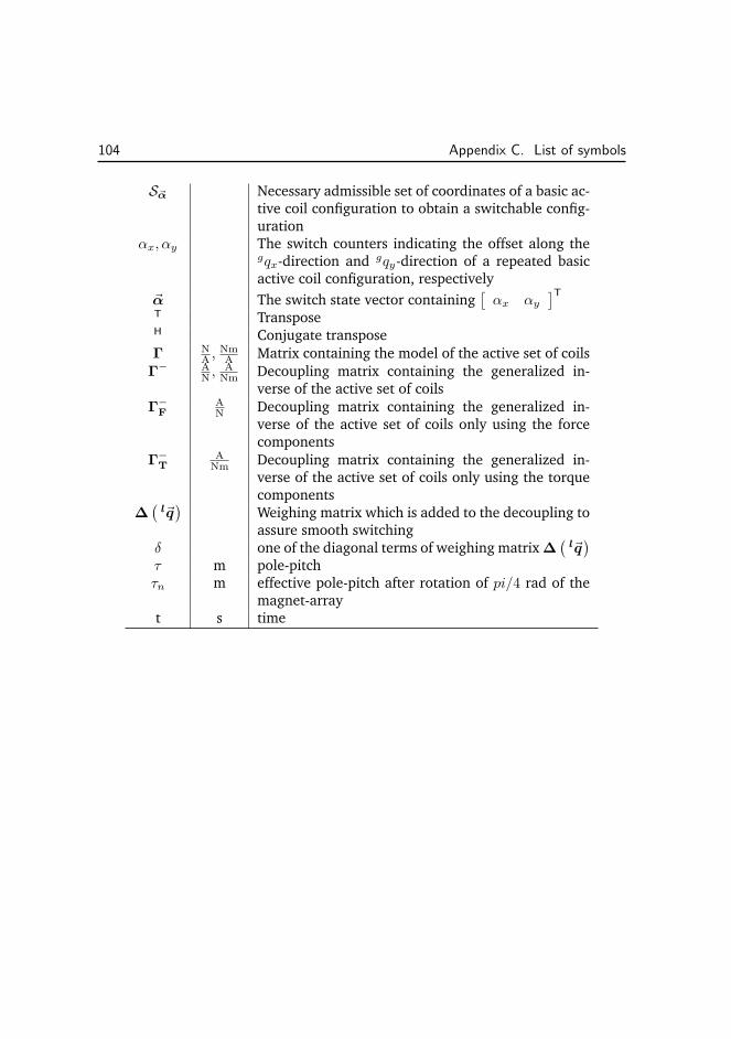
104 Appendix C. List of symbols
S~α Necessary admissible set of coordinates of a basic ac-tive coil configuration to obtain a switchable config-uration
αx, αy The switch counters indicating the offset along thegqx-direction and gqy-direction of a repeated basicactive coil configuration, respectively
~α The switch state vector containing[
αx αy]T
T TransposeH Conjugate transpose
ΓNA ,
NmA Matrix containing the model of the active set of coils
Γ− A
N ,A
Nm Decoupling matrix containing the generalized in-verse of the active set of coils
Γ−F
AN Decoupling matrix containing the generalized in-
verse of the active set of coils only using the forcecomponents
Γ−T
ANm Decoupling matrix containing the generalized in-
verse of the active set of coils only using the torquecomponents
∆(
l~q)
Weighing matrix which is added to the decoupling toassure smooth switching
δ one of the diagonal terms of weighing matrix ∆(
l~q)
τ m pole-pitchτn m effective pole-pitch after rotation of pi/4 rad of the
magnet-arrayt s time
Bibliography
[1] M. B. Binnard, “Six degree of freedom control of planar motors,” U.S. PatentApplication 2003/0 085 676, May 8, 2003.
[2] M. B. Binnard, “System and method to control planar motors,” U.S. Patent6,650,079, Nov. 18, 2003.
[3] M. S. Branicky, V. S. Borkar, and S. K. Mitter, “A unified famework for hy-brid control: Model and optimal control theory,” IEEE Trans. Automat. Contr.,vol. 43, pp. 31–45, Jan. 1998.
[4] J. C. Compter, “Electro-dynamic planar motor,” Precision Engineering, vol. 28,no. 2, pp. 171–180, Apr. 2004.
[5] J. C. Compter and P. C. M. Frissen, “Displacement device,” Patent WO01/18 944 A1, Mar. 15, 2001.
[6] J. C. Compter, P. C. M. Frissen, and J. van Eijk, “Displacement device,” PatentWO 2006/075 291 A2, Jul. 20, 2006.
[7] B. de Kraker and D. H. van Campen, Mechanical vibrations. The Netherlands:Shaker, 2001.
[8] R. E. Doherty and C. A. Nickle, “Synchronous machines - parts I and II - anextension of Blondel’s two reaction theory - steady state power angle charac-teristics,” AIEE Trans., vol. 45, pp. 912–942, Jun. 1926.
[9] R. E. Doherty and C. A. Nickle, “Synchronous machines - part III - torque anglecharacteristics under transient conditions,” AIEE Trans., vol. 46, pp. 1–18, Feb.1927.
105
106 Bibliography
[10] R. E. Doherty and C. A. Nickle, “Synchronous machines - part IV,” AIEE Trans.,vol. 47, pp. 457–492, Feb. 1928.
[11] R. E. Doherty and C. A. Nickle, “Three-phase short circuit synchronous ma-chines - V,” AIEE Trans., vol. 49, pp. 700–714, Apr. 1930.
[12] E. Durand, Magnetostatique. Paris, France: Masson et Cie, 1968.
[13] A. E. Fitzgerald, J. C Kingsley, and S. D. Umans, Electric Machinery, 6th ed.New York: McGraw-Hill, 2003.
[14] M. Gajdusek, J. de Boeij, A. A. H. Damen, and P. P. J. van den Bosch, “Con-tactless planar actuator with manipulator - experimental setup for control,” inProc. of the 6th international symposium on linear drives for industrial applica-
tions, Lille, France, Sep. 2007.
[15] A. J. Hazelton, M. B. Binnard, and J. M. Gery, “Electric motors and positioningdevices having moving magnet arrays and six degrees of freedom,” U.S. Patent6,208,045, Mar. 27, 2001.
[16] R. A. Horn and C. R. Johnson, Matrix analysis. Cambridge, UK: Cambridgeuniversity press, 1999.
[17] J. W. Jansen, “Magnetically levitated planar actuator with moving magnets:electromechanical analysis and design,” Ph.D. dissertation, Eindhoven Univer-sity of Technology, Nov. 2007.
[18] J. W. Jansen, E. A. Lomonova, A. J. A. Vandenput, and C. M. M. van Lierop,“Analytical model of a magnetically levitated linear actuator,” in Conference
Record of the 2005 Industry Applications Conference 40th Annual Meeting, HongKong, Oct. 2005, pp. 2107–2113.
[19] J. W. Jansen, E. A. Lomonova, A. J. A. Vandenput, and C. M. M. van Lierop,“Design flow for a six degree-of-freedom planar actuator,” in Proc. of th 3rd
IEEE Young Researchers Symposium in Electrical Power Engineering, Ghent, Bel-gium, Apr. 2006.
[20] J. W. Jansen, C. M. M. van Lierop, J. de Boeij, E. A. Lomonova, J. L. Duarte,and A. J. A. Vandenput, “Moving magnet multi-dof planar actuator technologywith contactless energy and data transfer,” in Proc. of the 6th international
symposium on linear drives for industrial applications, Lille, France, Sep. 2007.
Bibliography 107
[21] J. W. Jansen, C. M. M. van Lierop, and E. A. Lomonova, “Werkwijze voorhet vervaardigen van een vlakke actuator alsmede een vlakke actuator aldusvervaardigd,” Dutch Patent Application 1 029 246, Jun. 14, 2005.
[22] J. W. Jansen, C. M. M. van Lierop, E. A. Lomonova, and A. J. A. Vandenput,“Moving-magnet planar actuator with integrated active magnetic bearing,” inProc. of the ASPE 2006 annual meeting, Monterey, California, Oct. 2006, pp.119–122.
[23] J. W. Jansen, C. M. M. van Lierop, E. A. Lomonova, and A. J. A. Vanden-put, “Magnetically levitated planar actuator with moving magnets,” in IEEE
Int. Electric Machines and Drives Conference (IEMDC’07), Antalya, Turkey, May2007, pp. 272–278.
[24] J. W. Jansen, C. M. M. van Lierop, E. A. Lomonova, and A. J. A. Vandenput,“Modeling of magnetically levitated planar actuators with moving magnets,”IEEE Trans. Magn., vol. 43, no. 1, pp. 15–25, Jan. 2007.
[25] J. W. Jansen, C. M. M. van Lierop, E. A. Lomonova, and A. J. A. Vandenput,“Ironless magnetically levitated planar actuator,” J. Appl. Phys., in press.
[26] J. W. Jansen, C. M. M. van Lierop, E. A. Lomonova, and A. J. A. Vandenput,“Magnetically levitated planar actuator with moving magnets,” IEEE Trans.
Ind. Applicat., in press.
[27] K. Kemp and S. Wurm, “EUV lithography,” Comptes Rendus Physique, vol. 7,pp. 875–886, 2006.
[28] W. J. Kim, “High-precision planar magnetic levitation,” Ph.D. dissertation,Massachusetts Institute of Technology, 1997.
[29] W. J. Kim, D. L. Trumper, and J. H. Lang, “Modeling and vector control of aplanar magnetic levitator,” IEEE Trans. Ind. Applicat., vol. 34, no. 6, pp. 1254–1262, Nov./Dec. 1998.
[30] N. Korenaga, “Alignment apparatus and exposure apparatus using the same,”U.S. Patent 7,075,198, Jul. 11, 2006.
[31] P. J. McKerrow, Introduction to robotics. Syndney, Australia: Addison-WesleyPublishers Ltd., 1991.
[32] H. Nijmeijer and A. J. van der Schaft, Nonlinear dynamical control systems.New York: Springer, 1990.
108 Bibliography
[33] R. H. Park, “Two-reaction theory of synchronous machines - generalizedmethod of analysis - part I,” AIEE Trans., vol. 48, pp. 716–730, Jul. 1929.
[34] R. H. Park, “Two-reaction theory of synchronous machines - generalizedmethod of analysis - part II,” AIEE Trans., vol. 52, pp. 352–355, Jun. 1933.
[35] ACM Micro Service manual, Philips EMT, Eindhoven, Netherlands, 2001.
[36] W. Potze and P. C. M. Frissen, “Method for controlling an electric motor, con-trol unit and electric motor,” Patent WO 2006/054 243 A2, May 26, 2006.
[37] C. R. Rao and S. K. Mitra, Generalized inverse of matrices and its applications.Wiley, 1971.
[38] S. Skogestad and I. Postlethwaite, Multivariable feedback control. England:Wiley, 2005.
[39] H. M. J. R. Soemers, “The design of high performance manipulators,” in Proc.
of the 2001 IEEE/ASME Int. Conf. on Advanced Intelligent Mechatronics, Como,Italy, Jul. 2001, pp. 149–152.
[40] T. Teng, T. Ueda, S. Makinouchi, and B. Yuan, “Moving magnet type planarmotor control,” in Proc. of the 1st Int. Conf. on Positioning Technology, Hama-matsu, Japan, Jun. 2004, pp. 203–208.
[41] T. Ueta, B. Yuan, and T. C. Teng, “Moving magnet type planar motor control,”U.S. Patent Application 2003/0 102 722, Jun. 5, 2003.
[42] C. M. M. van Lierop, J. W. Jansen, A. A. H. Damen, E. A. Lomonova, P. P. J.van den Bosch, and A. J. A. Vandenput, “Model based commutation of a long-stroke magnetically levitated linear actuator,” in Conference record of the 2006
IEEE Industry Applications Conference 41st Annual Meeting, Tampa, Florida,Oct. 2006.
[43] C. M. M. van Lierop, J. W. Jansen, A. A. H. Damen, E. A. Lomonova, P. P. J.van den Bosch, and A. J. A. Vandenput, “Model based commutation of a long-stroke magnetically levitated linear actuator,” IEEE Trans. Ind. Applicat., underreview.
[44] C. M. M. van Lierop, J. W. Jansen, A. A. H. Damen, and P. P. J. van denBosch, “Control of multi-degree-of-freedom planar actuators,” in Proc. of the
2006 IEEE International Conference on Control Applications, CCA 2006, Mu-nich, Germany, Oct. 2006, pp. 2516–2521.

Bibliography 109
[45] C. M. M. van Lierop, J. W. Jansen, E. A. Lomonova, A. A. H. Damen, A. J. A.Vandenput, and P. P. J. van den Bosch, “Commutation of a magnetically levi-tated planar actuator with moving-magnets,” in Proc. of the 6th international
symposium on linear drives for industrial applications, Lille, France, Sep. 2007.
[46] C. M. M. van Lierop, J. W. Jansen, E. A. Lomonova, A. A. H. Damen, A. J. A.Vandenput, and P. P. J. van den Bosch, “Commutation of a magnetically levi-tated planar actuator with moving-magnets,” IEEJ Trans. Ind. Applicat., underreview.

110 Bibliography
Samenvatting
Dutch abstract
Systemen met meerdere mechanische vrijheidsgraden worden vaak geconstrueerdmet elektromechanische actuatoren met maar een vrijheidsgraad. Over het alge-meen beschikken deze actuatoren over een standaard, vaak geıntegreerd, com-mutatie (d.w.z. linearisatie- en ontkoppelings-) algoritme, welke de actuator vande noodzakelijke ingangssignalen voorziet. Het toepassen van dit commutatie-algoritme resulteert bij deze machines in gemakkelijke regeleigenschappen en re-latief simpele actuator begrenzingen. In sommige applicaties is het noodzakelijkom actuatoren toe te passen die meerdere vrijheidsgraden combineren om zo tege-moet te kunnen komen aan de steeds strengere eisen. Als gevolg van het inte-greren van vrijheidsgraden in een actuator, worden de commutatie en de regelingechter complexer. Het is daarom van het grootste belang om de regeltechniekvanaf een vroeg stadium in het ontwerpproces van deze actuatoren mee te ne-men. De twee belangrijkste bijdragen van dit proefschrift zijn het beschrijven vaneen nieuw commutatie-algoritme, maar vooral ook het toelichten van de daaruitvoortvloeiende ontwerpimplicaties.
Een magnetisch gelagerde planaire (in een vlak bewegende) actuator is eenvoorbeeld van een actuator waarin meerdere vrijheidsgraden gecombineerd zijn.Deze actuator kan gebruikt worden als alternatief voor xy-aandrijvingen die bestaanuit aan elkaar gekoppelde lineaire motoren. Deze aandrijvingen worden veelaltoegepast in industriele hoge precisie applicaties waarbij objecten in een vlak gepo-sitioneerd moeten worden. De planaire actuator is opgebouwd uit een stator meteen aaneenschakeling van spoelen waarboven een translator met een patroon vanpermanente magneten zweeft. De translator, het bewegende deel, wordt hierbijslechts ondersteund door magnetische velden. Door het magnetische lager moet detranslator echter actief gestabiliseerd worden in zes vrijheidsgraden. In dit proef-
111
112 Samenvatting - Dutch abstract
schrift wordt de dynamica, de commutatie en het regelontwerp beschreven van eenmagnetisch gelagerde planaire actuator met bewegende magneten. Het grootstevoordeel van deze actuator is dat er geen kabels nodig zijn van de vaste wereld naarde translator. Alleen de spoelen die zich onder het magneetoppervlak bevinden,kunnen een effectieve bijdrage aan de levitatie en voortstuwing van de translatorleveren. Daarom wordt er afhankelijk van de positie van de translator in het xy-vlak geschakeld tussen verschillende sets van actieve spoelen. Het schakelen tussenspoelen in combinatie met de volledig contactloze translator maakt, in principe, eenoneindige slag in het xy-vlak mogelijk.
Vanwege de integratie van de voortstuwing in het xy-vlak en de actieve mag-netische lagering is het niet mogelijk om gebruik te maken van standaard ontkop-pelstrategieen voor synchrone machines voor het ontkoppelen van de kracht- enkoppelcomponenten. Vandaar dat er een nieuw commutatie-algoritme is afgeleiddat de transformatie van de kracht- en koppelcomponenten, als functie van destromen door de spoelen en de positie en orientatie van het platform, inverteert.In dit proefschrift is er gekozen voor een model-gebaseerde commutatie en regel-aanpak, gebruik makend van een real-time analytisch model van de planaire actu-ator. Het real-time model is gebaseerd op analytische oplossingen van de Lorentzkracht- en koppelintegralen. Het nieuwe algoritme levert een optimale oplossing,in die zin dat het energieverbruik van de actuator wordt geminimaliseerd. Nogeen belangrijke bijdrage in dit proefschrift is de introductie van gladde positie af-hankelijke weegfuncties in het commutatie-algoritme. Deze functies resulteren ineen glad schakelgedrag tussen verschillende actieve groepen van spoelen. De re-sulterende stroomvorm door iedere individueel aangestuurde actieve spoel is sterkniet sinusvormig.
De model-gebaseerde aanpak, in combinatie met het nieuwe commutatie-algoritme, heeft een ontwerpmethode opgeleverd die de regelbaarheid van planaire-actuatortopologieen opneemt in de ontwerpfase. Met behulp van deze methodeworden verscheidene topologieen behandeld in dit proefschrift. Door de veran-derende hoeveelheid actieve spoelen tijdens het schakelen tussen de verschillendeactieve spoelgroepen, hangen de actuator begrenzingen af van de xy-positie van detranslator. Dit proefschrift bevat daarom ook een analyse van de haalbare accele-ratie als functie van de positie van de translator in combinatie met de begrenzingvan de stroomversterkers. Verder is het dynamische gedrag van het ontkoppeldesysteem geanalyseerd bij kleine fouten en is er een stabiliserende regelstructuurafgeleid.
Een van de ontwerpen van de planaire actuator, de HPPA (Herringbone Pat-tern Planar Actuator), is tot in meer detail uitgewerkt en is ook daadwerkelijkgebouwd. Deze actuator is vernoemd naar het spoelpatroon (gelegen in een vis-
Samenvatting - Dutch abstract 113
graat patroon). De stator bestaat uit een totaal van 84 spoelen, waarvan er tussende 15 en 24 gelijktijdig worden gebruikt voor de lagering en de voortstuwing vande translator. Het real-time model, het dynamische gedrag en het commutatie-algoritme zijn experimenteel geverifieerd met behulp van deze volledig operationeleactuator. De magnetisch gelagerde, planaire actuator met zes vrijheidsgraden enbewegende magneten (de HPPA) is ontwikkeld en getest en werkt naar behorenvolgens alle vooraf gestelde ontwerp- en prestatie-eisen.

114 Samenvatting - Dutch abstract
Dankwoord
Acknowledgements
Tijdens het afronden van dit proefschrift is het schrijven van een dankwoord eenprettige afleiding. Een project zoals dit staat of valt met een goede samenwerking.Vandaar dat ik als eerste mijn collega Helm Jansen wil bedanken voor de prettigesamenwerking van de afgelopen vier jaar. Je gedrevenheid om dit project tot eengoed einde te brengen, ook als het wel eens tegen zat, was een belangrijke motivatievoor mij om hetzelfde te doen. Ook ik had mij geen betere project partner kunnenwensen [17].
Natuurlijk wil ik ook mijn vriendin Chantal bedanken voor het vele geduld datze heeft moeten uitoefenen tijdens het afronden van mijn proefschrift. Je bent mijnrots in de branding. Ik ben erg blij met wat we, ondanks de turbulente periode, hetafgelopen jaar samen hebben bereikt.
Mijn familie heeft er de afgelopen vier jaar voor gezorgd dat er genoeg rustwas in mijn prive situatie om ongestoord te kunnen werken. Els, John en Willem:Bedankt dat ik altijd bij jullie aan kon kloppen als er iets was waar ik mee zat.Hoewel het vele klussen aan het huis veel tijd en energie in beslag heeft genomenwas het een aangename afwisseling ten opzichte van mijn taken als promovendus.In relatie tot mijn proefschrift wil ik mijn vader en Maarten van Dijk bedanken voorhet ontwerpen van de mooie kaften.
Verder wil ik Paul van den Bosch, Ad Damen, Andre Vandenput en ElenaLomonova bedanken voor de vrijheid en het vertrouwen in de afgelopen periode.Jullie enthousiasme met betrekking tot dit project heeft het mogelijk gemaakt ombinnen de gestelde periode een werkend prototype af te kunnen leveren.
Mijn commissieleden, Hans Butler, John Compter en Okko Bosgra wil ik be-danken voor het lezen van mijn proefschrift en de daaropvolgende discussies. Ookwil ik Michel Antal bedanken voor het zitting nemen in mijn commissie, het goed-
115
116 Dankwoord - Acknowledgements
keuren van mijn publicaties, en zijn inzet voor IOP-EMVT.Het succesvol realiseren van een werkend prototype was nooit gelukt zon-
der de inzet van diverse mensen. In het bijzonder wil ik daarom Marijn Uyt deWilligen bedanken voor de vele uren die hij heeft gestoken in het realiseren vaneen veilige en betrouwbare opstelling (en het aanhoren van onze verhalen). Ookwil ik Will Hendrix, Udo Bartzke en Ab Schrader bedanken voor hun inzet bij hetimplementeren van de regelopstelling en de protocollen. Een groot aantal compo-nenten moest speciaal voor deze opstelling worden ontwikkeld. De gemeenschap-pelijke technische dienst (GTD) van de technische universiteit Eindhoven heeft eenonmisbare bijdrage geleverd aan de ontwikkeling en de assemblage van de mecha-nica. Vooral dankzij de inzet en flexibiliteit van Jovita Moerel en Patrick de Laatis de samenwerking met de GTD soepel en succesvol verlopen. Vanuit het bedrijfs-leven wil ik Korneel Wijnands (Prodrive), Mark van den Broek (Vacuumschmelze),Peter Krechting (Tecnotion), Ad Vermeer (Assembleon) en Peter van Gils (ASML)bedanken voor hun inzet.
Verder zijn er nog een aantal stagiaires en afstudeerders die een bijdragehebben geleverd aan de opstelling. Hiervan wil ik in het bijzonder, Angelino Eij-germans, Justin van Essen, Jan Schellekens en Jochem Vissers bedanken.
Natuurlijk zijn er ook vele collega’s die ik wil bedanken. Allereerst wil iknatuurlijk mijn altijd aanwezige kamergenoot Andrej Jokic bedanken voor de veleleuke gesprekken. Dankzij jou viel het gelukkig een stuk minder op dat ik ook be-hoorlijk chaotisch ben. Ik hoop alleen wel dat we vanaf nu iets minder vaak opkantoor te vinden zijn. Graag wil ik langs deze weg ook mijn collega promovendi,Aleksandar, Anton, Bart, Femke, Hans, Heico, Jasper, Jeroen, John, Juraj, Lauren-tiu, Leo, Maarten, Mark, Michal, Michiel, Mircea, Patricia, Patrick, Paul en Satyabedanken. In het bijzonder wil ik Mark en Maarten bedanken voor de leuke tijd diewe hebben gehad tijdens conferenties, John voor de discussies over het bouwen vanhuizen en Mircea voor de ondertitel van dit proefschrift. Mijn collega paranimf enbijna kamergenoot Paul wil ik bedanken voor de leuke tijd en het ongewild bijwo-nen van de discussies tussen Helm en mij. Siep Weiland wil ik bedanken voor zijnwiskundig advies. Natuurlijk wil ik ook Barbara bedanken voor de leuke uitjes envoor de hulp bij al mijn financiele, organisatorische en administratieve problemen.
Ook wil ik langs deze weg al mijn vrienden, die ik de afgelopen tijd hebmoeten verwaarlozen, bedanken. Jullie gaan weer meer van mij horen.
Een raar fenomeen is dat het meest toegankelijke en over het algemeen meestgelezen deel, namelijk het dankwoord, vaak opgenomen wordt aan het eind vaneen proefschrift. Tot slot wil ik dus alle mensen bedanken die de moeite hebbengenomen om dit deel van mijn proefschrift te bereiken door bij de titelpagina tebeginnen en het proefschrift van voor tot achter door te lezen.
Curriculum Vitae
Nelis van Lierop was born in Eindhoven, the Netherlands, on the 11th of March in1978. He attended secondary school at the Pastoor Aelen-mavo (MAVO) in Eerselfrom 1992 until 1994 and at the Rythovius College (HAVO) in Eersel from 1994until 1996. During this period he received the third price at the ”Nationale wedstrijdvoor jonge onderzoekers” (a national, Dutch, contest for young researchers).
He then started studying electrical engineering in Eindhoven at the FontysHogescholen (HTS) in 1996. His internship at the physics department of the Eind-hoven University of Technology comprised of the design of a modulator for a lin-ear micro-bunch particle accelerator. His graduation project took place at PhilipsLighting and concerned the design of a dual output power converter for a lightapplication. He received his B.Sc.-degree in electrical engineering in 2000.
In 2000, he started studying electrical engineering at the Eindhoven Universityof technology. His graduation project within the control systems group took placeat the physics department of the same university, and concerned ”The influence ofamplitude and phase variations on a resonant cavity”. The research comprised ofthe analysis of the effect of amplitude and phase variations on the output power ofa linear particle accelerator. The results of this analysis and the designed modulator(during his internship) have been successfully applied to several accelerators. Hereceived his (Cum Laude) M.Sc.-degree in electrical engineering in 2003.
From October 2003 to Januari 2008, he pursued his Ph.D. degree in the con-trol systems group of the department of electrical engineering at the EindhovenUniversity of Technology. The topic of his Ph.D. research was a ”Magnetically Levi-tated Planar Actuator with Moving Magnets” where he focussed on the ”Dynamics,Commutation and Control Design”. During his Ph.D. research he also received thecourse certificate of the Dutch Institute of Systems and Control DISC for completinga required number of postgraduate courses.
Nelis’ personal interests are art and listening to, performing and composing(piano) music. He played in several bands (e.g. GuessStation and In-Tension).
117