
Catalytic applications of a versatile magnetically separable Fe-Mo nanocatalyst
Upload
khangminh22Category
view
0download
0
Detection of Magnetically Trapped Neutrons:
Liquid Helium as a Scintillator
A thesis presented
by
Daniel Nicholas McKinsey
to
The Department of Physics
in partial fulfillment of the requirements
for the degree of
Doctor of Philosophy
in the subject of
Physics
Harvard University
Cambridge, Massachusetts
February 2002
c©2002 - Daniel Nicholas McKinsey
All rights reserved.

To my parents

Thesis advisor Author
John Morrissey Doyle Daniel Nicholas McKinsey
Detection of Magnetically Trapped Neutrons:
Liquid Helium as a Scintillator
Abstract
Herein, we describe the magnetic trapping of ultracold neutrons and the design
and testing of an experiment to measure the neutron beta-decay lifetime. In this
approach, ultracold neutrons are loaded into a magnetic trap through the superther-
mal effect in liquid helium, and then the same helium bath is used as a scintillator
to detect decay of the trapped neutrons. The design of the experiment is described
in detail, with particular emphasis given to the technical development of charged
particle detectors based on liquid helium and to the construction of a large, deep su-
perconducting magnetic trap. Trapping of ultracold neutrons has been demonstrated
with a statistical significance of 5.4 σ.

Contents
Title Page . . . . . . . . . . . . . . . . . . . . . . . . . . . . . . . . . . . . iDedication . . . . . . . . . . . . . . . . . . . . . . . . . . . . . . . . . . . . iiiAbstract . . . . . . . . . . . . . . . . . . . . . . . . . . . . . . . . . . . . . ivTable of Contents . . . . . . . . . . . . . . . . . . . . . . . . . . . . . . . . vAcknowledgements . . . . . . . . . . . . . . . . . . . . . . . . . . . . . . . xi
1 Introduction 11.1 Ultracold Neutrons . . . . . . . . . . . . . . . . . . . . . . . . . . . . 11.2 The Neutron Lifetime . . . . . . . . . . . . . . . . . . . . . . . . . . . 21.3 Previous experiments . . . . . . . . . . . . . . . . . . . . . . . . . . . 121.4 Magnetic Trapping of Neutrons to Measure the Neutron Lifetime . . 20
2 Scintillations in Liquid Helium: History and Motivation 322.1 Historical Background . . . . . . . . . . . . . . . . . . . . . . . . . . 322.2 Fundamental Physics Experiments Using
Liquid Helium as a Scintillator . . . . . . . . . . . . . . . . . . . . . . 39
3 Detector Development 423.1 Fluor Development . . . . . . . . . . . . . . . . . . . . . . . . . . . . 433.2 Fiber Cells . . . . . . . . . . . . . . . . . . . . . . . . . . . . . . . . . 523.3 Tube Cells . . . . . . . . . . . . . . . . . . . . . . . . . . . . . . . . . 593.4 Gore-tex Cells . . . . . . . . . . . . . . . . . . . . . . . . . . . . . . . 68
4 The Physics of Liquid Helium Scintillations 714.1 Prompt Scintillation . . . . . . . . . . . . . . . . . . . . . . . . . . . 724.2 Afterpulsing . . . . . . . . . . . . . . . . . . . . . . . . . . . . . . . . 744.3 Helium Phosphorescence . . . . . . . . . . . . . . . . . . . . . . . . . 834.4 Summary of Helium Scintillations . . . . . . . . . . . . . . . . . . . . 88
5 Experimental Apparatus 915.1 Overview . . . . . . . . . . . . . . . . . . . . . . . . . . . . . . . . . . 915.2 The Neutron Beam . . . . . . . . . . . . . . . . . . . . . . . . . . . . 925.3 Dewar and Cryogenics . . . . . . . . . . . . . . . . . . . . . . . . . . 945.4 The Detection Insert . . . . . . . . . . . . . . . . . . . . . . . . . . . 106
v
5.5 The Magnetic Trap . . . . . . . . . . . . . . . . . . . . . . . . . . . . 1195.6 Background Suppression . . . . . . . . . . . . . . . . . . . . . . . . . 1285.7 Data Acquisition . . . . . . . . . . . . . . . . . . . . . . . . . . . . . 132
6 Data Analysis 1356.1 Data Collection . . . . . . . . . . . . . . . . . . . . . . . . . . . . . . 1356.2 Data Cuts and Thresholds . . . . . . . . . . . . . . . . . . . . . . . . 1366.3 Backgrounds . . . . . . . . . . . . . . . . . . . . . . . . . . . . . . . . 1396.4 Data . . . . . . . . . . . . . . . . . . . . . . . . . . . . . . . . . . . . 1426.5 Analysis . . . . . . . . . . . . . . . . . . . . . . . . . . . . . . . . . . 1436.6 Discussion . . . . . . . . . . . . . . . . . . . . . . . . . . . . . . . . . 150
7 Conclusions and Recommendations 1577.1 Progress in Cycle 8 . . . . . . . . . . . . . . . . . . . . . . . . . . . . 1577.2 Lessons From Cycle 8 . . . . . . . . . . . . . . . . . . . . . . . . . . . 1587.3 Recommendations For Future Work . . . . . . . . . . . . . . . . . . . 160
A Data Analysis Software 171
Bibliography 173
vi
List of Figures
1.1 Neutron beta decay . . . . . . . . . . . . . . . . . . . . . . . . . . . . 41.2 Scheme for calculating angular correlation coefficients . . . . . . . . . 71.3 CKM Unitarity . . . . . . . . . . . . . . . . . . . . . . . . . . . . . . 111.4 Previous measurements of the neutron lifetime . . . . . . . . . . . . . 141.5 Schematic of a beam lifetime measurement. . . . . . . . . . . . . . . . 151.6 A sketch of the idea of the NESTOR experiment. . . . . . . . . . . . 161.7 Storing neutrons in a bottle . . . . . . . . . . . . . . . . . . . . . . . 191.8 Currents in an Ioffe trap . . . . . . . . . . . . . . . . . . . . . . . . . 221.9 The superthermal process . . . . . . . . . . . . . . . . . . . . . . . . 261.10 Detecting neutron decay . . . . . . . . . . . . . . . . . . . . . . . . . 28
2.1 Scintillation spectrum of electron-bombarded liquid helium . . . . . . 362.2 Helium molecular potentials . . . . . . . . . . . . . . . . . . . . . . . 37
3.1 Tetraphenyl Butadiene . . . . . . . . . . . . . . . . . . . . . . . . . . 443.2 Fluorescence Efficiency Rig . . . . . . . . . . . . . . . . . . . . . . . . 463.3 Fluorescence efficiencies of evaporated films. . . . . . . . . . . . . . . 483.4 Fluorescence efficiencies of sprayed films . . . . . . . . . . . . . . . . 483.5 Fluorescence efficiencies of doped plastic films . . . . . . . . . . . . . 503.6 Fiber cell construction . . . . . . . . . . . . . . . . . . . . . . . . . . 533.7 Triplet Molecule Rig . . . . . . . . . . . . . . . . . . . . . . . . . . . 563.8 Acrylic tube-based trapped neutron detection . . . . . . . . . . . . . 593.9 Gain dispersion of the Burle 8850 PMT . . . . . . . . . . . . . . . . . 613.10 Cell Testing Rig . . . . . . . . . . . . . . . . . . . . . . . . . . . . . . 623.11 Neutron spectrum . . . . . . . . . . . . . . . . . . . . . . . . . . . . . 653.12 Calibrations of tube cells . . . . . . . . . . . . . . . . . . . . . . . . . 663.13 Fluorescence signal versus position . . . . . . . . . . . . . . . . . . . 67
4.1 Beta induced afterpulsing . . . . . . . . . . . . . . . . . . . . . . . . 764.2 Alpha induced afterpulsing . . . . . . . . . . . . . . . . . . . . . . . . 774.3 Alpha induced afterpulsing . . . . . . . . . . . . . . . . . . . . . . . . 814.4 Triplet Molecule Results . . . . . . . . . . . . . . . . . . . . . . . . . 884.5 Chemical processes following helium ionization . . . . . . . . . . . . . 90
vii
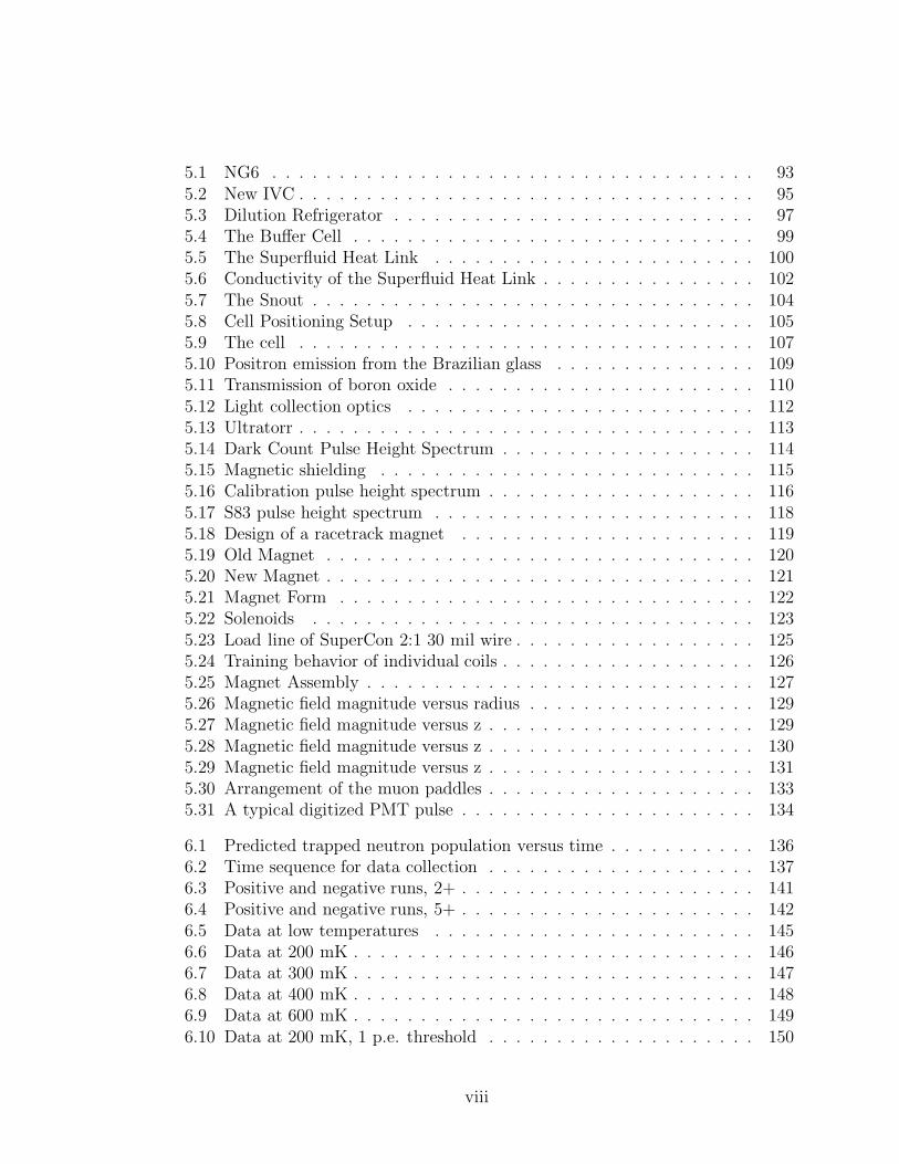
5.1 NG6 . . . . . . . . . . . . . . . . . . . . . . . . . . . . . . . . . . . . 935.2 New IVC . . . . . . . . . . . . . . . . . . . . . . . . . . . . . . . . . . 955.3 Dilution Refrigerator . . . . . . . . . . . . . . . . . . . . . . . . . . . 975.4 The Buffer Cell . . . . . . . . . . . . . . . . . . . . . . . . . . . . . . 995.5 The Superfluid Heat Link . . . . . . . . . . . . . . . . . . . . . . . . 1005.6 Conductivity of the Superfluid Heat Link . . . . . . . . . . . . . . . . 1025.7 The Snout . . . . . . . . . . . . . . . . . . . . . . . . . . . . . . . . . 1045.8 Cell Positioning Setup . . . . . . . . . . . . . . . . . . . . . . . . . . 1055.9 The cell . . . . . . . . . . . . . . . . . . . . . . . . . . . . . . . . . . 1075.10 Positron emission from the Brazilian glass . . . . . . . . . . . . . . . 1095.11 Transmission of boron oxide . . . . . . . . . . . . . . . . . . . . . . . 1105.12 Light collection optics . . . . . . . . . . . . . . . . . . . . . . . . . . 1125.13 Ultratorr . . . . . . . . . . . . . . . . . . . . . . . . . . . . . . . . . . 1135.14 Dark Count Pulse Height Spectrum . . . . . . . . . . . . . . . . . . . 1145.15 Magnetic shielding . . . . . . . . . . . . . . . . . . . . . . . . . . . . 1155.16 Calibration pulse height spectrum . . . . . . . . . . . . . . . . . . . . 1165.17 S83 pulse height spectrum . . . . . . . . . . . . . . . . . . . . . . . . 1185.18 Design of a racetrack magnet . . . . . . . . . . . . . . . . . . . . . . 1195.19 Old Magnet . . . . . . . . . . . . . . . . . . . . . . . . . . . . . . . . 1205.20 New Magnet . . . . . . . . . . . . . . . . . . . . . . . . . . . . . . . . 1215.21 Magnet Form . . . . . . . . . . . . . . . . . . . . . . . . . . . . . . . 1225.22 Solenoids . . . . . . . . . . . . . . . . . . . . . . . . . . . . . . . . . 1235.23 Load line of SuperCon 2:1 30 mil wire . . . . . . . . . . . . . . . . . . 1255.24 Training behavior of individual coils . . . . . . . . . . . . . . . . . . . 1265.25 Magnet Assembly . . . . . . . . . . . . . . . . . . . . . . . . . . . . . 1275.26 Magnetic field magnitude versus radius . . . . . . . . . . . . . . . . . 1295.27 Magnetic field magnitude versus z . . . . . . . . . . . . . . . . . . . . 1295.28 Magnetic field magnitude versus z . . . . . . . . . . . . . . . . . . . . 1305.29 Magnetic field magnitude versus z . . . . . . . . . . . . . . . . . . . . 1315.30 Arrangement of the muon paddles . . . . . . . . . . . . . . . . . . . . 1335.31 A typical digitized PMT pulse . . . . . . . . . . . . . . . . . . . . . . 134
6.1 Predicted trapped neutron population versus time . . . . . . . . . . . 1366.2 Time sequence for data collection . . . . . . . . . . . . . . . . . . . . 1376.3 Positive and negative runs, 2+ . . . . . . . . . . . . . . . . . . . . . . 1416.4 Positive and negative runs, 5+ . . . . . . . . . . . . . . . . . . . . . . 1426.5 Data at low temperatures . . . . . . . . . . . . . . . . . . . . . . . . 1456.6 Data at 200 mK . . . . . . . . . . . . . . . . . . . . . . . . . . . . . . 1466.7 Data at 300 mK . . . . . . . . . . . . . . . . . . . . . . . . . . . . . . 1476.8 Data at 400 mK . . . . . . . . . . . . . . . . . . . . . . . . . . . . . . 1486.9 Data at 600 mK . . . . . . . . . . . . . . . . . . . . . . . . . . . . . . 1496.10 Data at 200 mK, 1 p.e. threshold . . . . . . . . . . . . . . . . . . . . 150
viii

6.11 Data at 750 mK . . . . . . . . . . . . . . . . . . . . . . . . . . . . . . 1516.12 Data at 1.1 K . . . . . . . . . . . . . . . . . . . . . . . . . . . . . . . 1526.13 Decay intensity versus temperature . . . . . . . . . . . . . . . . . . . 1536.14 Decay rate versus temperature . . . . . . . . . . . . . . . . . . . . . . 1536.15 Helium-3 data . . . . . . . . . . . . . . . . . . . . . . . . . . . . . . . 1546.16 Helium-3 data, 1 p.e. threshold . . . . . . . . . . . . . . . . . . . . . 155
7.1 A possible future design . . . . . . . . . . . . . . . . . . . . . . . . . 1617.2 KEK magnet cross-section . . . . . . . . . . . . . . . . . . . . . . . . 1677.3 Load lines for the KEK magnet . . . . . . . . . . . . . . . . . . . . . 169
ix

List of Tables
1.1 UCN properties . . . . . . . . . . . . . . . . . . . . . . . . . . . . . . 21.2 UCN interactions . . . . . . . . . . . . . . . . . . . . . . . . . . . . . 31.3 Measurements of λ . . . . . . . . . . . . . . . . . . . . . . . . . . . . 81.4 Neutron lifetime measurements . . . . . . . . . . . . . . . . . . . . . 131.5 UCN material potentials . . . . . . . . . . . . . . . . . . . . . . . . . 18
3.1 Values of the fluorescent efficiencies of optimized evaporated films rel-ative to that of sodium salicylate. . . . . . . . . . . . . . . . . . . . . 49
3.2 Maximum values for the relative fluorescent efficiencies of doped plasticfilms relative to that of sodium salicylate. . . . . . . . . . . . . . . . . 49
3.3 Fiber cell tests . . . . . . . . . . . . . . . . . . . . . . . . . . . . . . 543.4 Tube cell tests . . . . . . . . . . . . . . . . . . . . . . . . . . . . . . . 643.5 Summary of detector efficiencies . . . . . . . . . . . . . . . . . . . . . 70
5.1 Thermal conductance of the superfluid helium heatlink . . . . . . . . 101
6.1 Thresholds as a function of photoelectron number . . . . . . . . . . . 1386.2 Constant background due to helium . . . . . . . . . . . . . . . . . . . 1406.3 calendar . . . . . . . . . . . . . . . . . . . . . . . . . . . . . . . . . . 1436.4 Signal vs. threshold . . . . . . . . . . . . . . . . . . . . . . . . . . . . 144
x
Acknowledgements
My greatest thanks goes to John Doyle, for teaching me most of what I know
about experimental physics and being a physicist, and for supporting me in every
way throughout graduate school.
I am also tremendously grateful to Paul Huffman, whose enormously capable and
willing support extended into every facet of laboratory work. I would also like to
thank Paul for teaching me so much about low temperature work, and for his careful
and constructive reading of this manuscript.
Special thanks to Bob Golub, whose genius and vision made this work possible,
and for telling us when we were doing it all wrong.
Appreciation is also extended to James Butterworth, for patience and intelligence,
and teaching me about cryogenics in my early years of graduate school.
I would also like to thank my fellow graduate students on this experiment; we
suffered together through endless late nights and leaky dewars. Carlo Mattoni (my
“twin” in so many ways), radiated competence and willingness to help throughout
graduate school, and was a constant source of industry and comradeship. Sergei
Dzhosyuk deserves special mention for his natural competence, thorough industri-
ousness, and unflagging good humor. Liang Yang was a neverending source of quiet
competence; much of the success of this latest incarnation of the experiment is due to
his work. Clint Brome, Bob Michniak, and Kyle Alvine also contributed significantly
to the experiment.
Thanks to Jonathan Weinstein, for his exceptional sense of humor, and for our
friendship throughout graduate school.
My appreciation also goes out to my fellow students in the Doyle Lab, for mak-
xi

ing the basement of Lyman a pleasant but vigorous environment for work and play.
Harvard has been a fertile environment for my intellectual growth, and the numer-
ous lunchtime discussions aided my education and made my time at Harvard more
pleasant.
Thanks to the folks at NIST for creating a supportive environment at the NCNR.
I am indebted also to Klaus Habicht for his early, careful work on the detection
of helium scintillations.
I also wish to thank Eva Allan; her love sustained me through the late months of
the experiment and the frenzied writing of this thesis.
This thesis is dedicated to my parents. I thank them for their total, unqualified
support and enthusiasm.
xii

Chapter 1
Introduction
1.1 Ultracold Neutrons
The term “ultracold neutrons” (also known as UCN) refers to neutrons whose energies
are so low (∼ 100 neV, T ∼ 1 mK) that they can be confined within an experimental
apparatus using material walls. This is possible when the neutron cannot overcome
the aggregate Fermi potential of the wall and the wavelength of the neutron (∼ 80 nm
at 1 mK) is large compared to the interatomic spacing. In this case the material walls
present a step potential with a height
Vmat = 2π�2Na/mn,
where N is the number density of atoms, a is the coherent neutron scattering length,
and mn is the mass of the neutron[1]. For many wall materials the UCN can bounce
off the walls many thousands of times before being absorbed; bottles made form these
materals can store UCN for many minutes before they decay, are absorbed, or scatter
inelastically. Some properties of a 1 mK neutron are listed in Table 1.1.
UCN are also of low enough energy to be affected strongly by gravity and exper-
1

Chapter 1. Introduction 2
Table 1.1: A summary of the properties of a 1 mK neutron.
Property Expression Value for a 1 mK UCN
Mass mn 1.675 ×10⁻²⁷ kg
Energy 32kBT 2.07 × 10⁻²⁶ J (129 neV)
Speed (2E/m)1/2 4.97 m/s
Wavelength h/mnv 79.6 nm
Magnetic moment -1.91 µN 9.65× 10⁻²⁷ J/T
imentally accessible magnetic fields. The strengths of these interactions are summa-
rized in Table 1.2. The rich array of experimental tools available for the investigation
of UCN makes possible many imaginative and interesting experiments.
UCN are particularly well suited for many experiments in fundamental physics
where it is beneficial to keep neutrons in an apparatus for a long time. While thermal
neutrons (T ∼ 300 K, v ∼ 2700 m/s) or cold neutrons (T ∼ 30 K, v ∼ 860 m/s) spend
very little time (∼ ms) in an experimental apparatus, ultracold neutrons, through
material, magnetic, or gravitational confinement, can be stored for times limited
primarily by the neutron lifetime (τn ∼ 900 s). Of particular interest are the search
for the neutron electric dipole moment, in which long neutron coherence times are
required, and the accurate measurement of the neutron lifetime, where neutron losses
by processes other than beta decay must be suppressed.
1.2 The Neutron Lifetime
The neutron is the simplest unstable nucleus. The relationship between the neutron
lifetime τn and the fundamental constants of nuclear decay, ga and gv, is particularly

Chapter 1. Introduction 3
Table 1.2: A summary of UCN interactions.
Interaction Expression Limit for a 1 mK UCN
Gravitational Egrav = mgh h = 1.26 m
Magnetic Vmag = µB B = 2.15 T
Strong Vmat = 2π�2Na/mn Na = 5.01 × 1023cm−3 fm
simple, with few theoretical uncertainties. This makes the neutron a unique labora-
tory for studies of the weak force. The neutron lifetime is an important parameter in
evaluating the unitarity of the CKM quark mixing matrix.
The neutron lifetime is also interesting in the context of Big Bang Nucleosyn-
thesis (BBN), determining the production of light elements in the early universe.
Uncertainty in the neutron lifetime is the most significant theoretical uncertainty in
estimations of 4He production in the Big Bang[2].
Neutron Beta Decay
Neutrons and protons make up the nuclei of ordinary matter, and are each made of
three quarks (one up and two down in the neutron, two up and one down in the
proton). While protons are stable (τp > 6.7 × 1032 years[3]), free neutrons are not.
A free neutron decays in about 15 minutes to a proton, an electron, and an electron
anti-neutrino:
n → p + e− + νe + 782.6 keV.
This decay is possible because the mass of the neutron (mn = 939.5656MeV/c2)
is greater than the masses of all three products combined. The mass of the pro-
ton (mp = 938.2720MeV/c2) is slightly less than the neutron mass, the difference

Chapter 1. Introduction 4
arising from difference in electrostatic potential energy and from the mass differ-
ence between the up quark and the down quark. The mass of the electron is small
(me = 0.511MeV/c2), and the mass of the electron antineutrino is small indeed
(mν � 1 eV). The net energy difference in the decay is 782.6 keV, and is released
as kinetic energy of the three decay products. According to the Standard Model, the
decay is mediated by the charged W− boson as shown in Figure 1.1.
n
W e –
p +
νe
–
Figure 1.1: The neutron decays into a proton, an electron, and an electron antineu-trino through the mediation of a W− boson.
To understand the mechanism of neutron beta decay and learn of the implications
of measuring the neutron lifetime, one must comprehend the theory of electroweak
interactions. This theory merges the theories of electromagnetism and the weak
interaction. Like quantum electrodynamics (the relativistic, renormalizable theory of
electromagnetism), electroweak theory assumes a current that couples to itself at a
single space-time point in the limit of low momentum transfer. But unlike quantum
electrodynamics, which assumes a vector coupling γλ, electroweak theory assumes a
Chapter 1. Introduction 5
combination of vector and axial vector coupling, γλ(1 − γ5). The Lagrangian density
is given by
L = − GF
2√
2(JλJ
λ† + Jλ†Jλ).
The weak current Jλ has both a leptonic and a hadronic part:
Jλ = jlλ + jh
λ
where
jlλ = eγλ(1 − γ5)νe + µγλ(1 − γ5)νµ + τ γλ(1 − γ5)ντ
couples leptons (electrons, muons, and tauons) to their respective neutrinos and
jhλ = d′γλ(1 − γ5)u + s′γλ(1 − γ5)c + b′γλ(1 − γ5)t
couples quarks to each other. That is, the weak interaction can change quarks from
one kind to another, and simultaneously turn leptons into neutrinos.
Because the quark mass eigenstates are not the same as the eigenstates of the weak
force, the d, s, and b quarks are replaced by the weak interaction quark eigenstates
of d′, s′, and b′, which are obtained by transforming with the Cabibbo-Kobayashi-
Maskawa quark mixing matrix:
d′
s′
b′
=
Vud Vus Vub
Vcd Vcs Vcb
Vtd Vts Vtb
d
s
b
.
In the case of neutron decay, a neutron turns into a proton, electron, and antineu-
trino. The parts of the Lagrangian that pertain to other particles can be neglected
to obtain:
L =GF
2√
2< p|jh
λ |n > eγλ(1 − γ5)νe
Chapter 1. Introduction 6
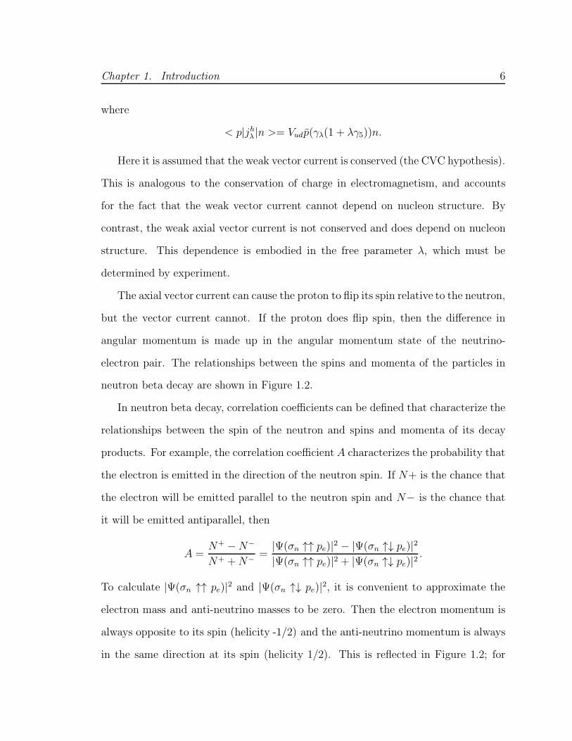
where
< p|jhλ |n >= Vudp(γλ(1 + λγ5))n.
Here it is assumed that the weak vector current is conserved (the CVC hypothesis).
This is analogous to the conservation of charge in electromagnetism, and accounts
for the fact that the weak vector current cannot depend on nucleon structure. By
contrast, the weak axial vector current is not conserved and does depend on nucleon
structure. This dependence is embodied in the free parameter λ, which must be
determined by experiment.
The axial vector current can cause the proton to flip its spin relative to the neutron,
but the vector current cannot. If the proton does flip spin, then the difference in
angular momentum is made up in the angular momentum state of the neutrino-
electron pair. The relationships between the spins and momenta of the particles in
neutron beta decay are shown in Figure 1.2.
In neutron beta decay, correlation coefficients can be defined that characterize the
relationships between the spin of the neutron and spins and momenta of its decay
products. For example, the correlation coefficient A characterizes the probability that
the electron is emitted in the direction of the neutron spin. If N+ is the chance that
the electron will be emitted parallel to the neutron spin and N− is the chance that
it will be emitted antiparallel, then
A =N+ − N−
N+ + N− =|Ψ(σn ↑↑ pe)|2 − |Ψ(σn ↑↓ pe)|2|Ψ(σn ↑↑ pe)|2 + |Ψ(σn ↑↓ pe)|2
.
To calculate |Ψ(σn ↑↑ pe)|2 and |Ψ(σn ↑↓ pe)|2, it is convenient to approximate the
electron mass and anti-neutrino masses to be zero. Then the electron momentum is
always opposite to its spin (helicity -1/2) and the anti-neutrino momentum is always
in the same direction at its spin (helicity 1/2). This is reflected in Figure 1.2; for

Chapter 1. Introduction 7
Vector
Axial vectorx λ
x √2 λ
Neutron: Proton: Leptons:
1 √2
1 √2
{ - }
{ + }
|S = 0, m = 0 >
|S = 1, m = 0 >
|S = 1, m = 1 >
Figure 1.2: Simple scheme for calculating angular correlation coefficients a, A, andB. Wide arrows indicate spin direction, thin arrows indicate direction of momenta.Numerical factors are two- and three- spin one half coupling coefficients. This figureis taken from reference [4].
the electron, the wide arrow indicating spin is always in the opposite direction to the
thin arrow indicating momentum, and for the anti-neutrino the opposite is the case.
Adding together the amplitudes for the electron to be emitted parallel to the
neutron spin, then multiplying by the complex conjugate, we find:
|Ψ(σn ↑↑ pe)|2 = | 1√2(1 − λ)|2 =
1
2(1 − 2Re(λ) + |λ|2).
Similarly, we can calculate the chance that the electron will be emitted anti-parallel
to the neutron spin. In the this case the proton may flip spin; this is treated as a
separate outcome and squared separately:
|Ψ(σn ↑↓ pe)|2 = | 1√2(−1 − λ)|2 + |2λ|2 =
1
2(1 + 2Re(λ) + |λ|2) + 2|λ|2

Chapter 1. Introduction 8
Table 1.3: A summary of previous measurements of the neutron beta-decay asymme-try. These are the four measurements used by the PDG to evaluate CKM unitarity.[5]
Measured λ Authors Reference
−1.2735 ± 0.0021 Reich et al. [6]
−1.266 ± 0.004 Liaud et al. [7]
−1.2594 ± 0.0038 Yerozolimsky et al. [8]
−1.262 ± 0.005 Bopp et al. [9]
One then has
Aexp =N+ − N−
N+ + N− =|Ψ(σn ↑↑ pe)|2 − |Ψ(σn ↑↓ pe)|2|Ψ(σn ↑↑ pe)|2 + |Ψ(σn ↑↓ pe)|2
= −2|λ|2 + Re(λ)
1 + 3|λ|2 .
Other correlation coefficients relate the electron and neutrino momenta (a), the
neutron spin and neutrino momentum (B), and the triple product of the neutron
spin, electron momentum, and neutrino momentum (D). Like A, these coefficients
can be expressed in terms of λ:
a =1 − |λ|21 + 3|λ|2 (1.1)
A = −2|λ|2 + Re(λ)
1 + 3|λ|2 (1.2)
B = 2|λ|2 + Re(λ)
1 + 3|λ|2 (1.3)
D = 2Im(λ)
1 + 3|λ|2 (1.4)
Obviously, any experimental measurements of these correlation coefficients should
all yield consistent values of λ; discepancies could indicate physics beyond the Stan-
dard Model. At this time, experiments measuring A give the most accurate estimates
of λ; these measurements are summarized in Table 1.3.

Chapter 1. Introduction 9
The matrix element for neutron decay can be written in terms of the correlation
coefficients described above. Expressed as a decay rate dW , one finds that
dW = F (Ee)
{1 + a
�pe �pν
EeEν+ b
m
Ee+ 〈 �σn〉 · (A
�pν
Ee+ B
�pν
Ee+ D
�pe × �pν
EeEν)
}.
By averaging dW over spins and integrating over the energies of the decay prod-
ucts, one finds that
τ−1 =m5
ec4
2π3�7fR(g2
v + 3g3a)
where τ is the neutron lifetime, gv = VudGF , and ga = VudλGF . The phase-space
factor
fR = 1.71465 ± 0.00015
can be calculated including radiative corrections[10]. The factor of 3g2a derives from
the 3 possible spin states of the lepton products in the case of axial vector coupling.
CKM Unitarity
Measurements of the neutron lifetime and any beta decay asymmetry allow one to
determine the fundamental constants of the weak interaction. By comparing the
constants determined through neutron beta decay with those measured in other pro-
cesses, one can test the consistency of the theoretical framework of the Standard
Model. In addition, one can test the unitarity of the CKM quark mixing matrix, that
is, whether V †V = I . Unitarity implies that
|Vud|2 + |Vus|2 + |Vub|2 = 1,
and this can be tested experimentally. By measuring the rates of the decays
B → π�ν� and B → ρ�ν�, |Vub| was measured to be 3.3 ± 0.4 ± 0.7 × 10⁻³[11]. In
a similar fashion, from the rate of the beta decay of the kaon, K+ → π0e+νe, |Vus|

Chapter 1. Introduction 10
was determined to be 0.2196 ± 0.0023[12]. The limiting uncertainty in determining
the unitarity of the CKM matrix is the measurement of Vud, determined through
0+ → 0+ nuclear decay, neutron decay, or π− decay. As seen in Figure 1.3, the value
of Vud measured through 0+ → 0+ nuclear decay is slightly less than unitarity would
imply. The uncertainty from 0+ → 0+ nuclear decay is primarily theoretical, while
testing unitarity through neutron decay is primarily experimental. Extracting Vud
through neutron decay requires two measurements: the neutron lifetime τn and a
measurement of λ, usually done by determining A. Recent measurements of A vary
substantially; depending on which measurement of A one chooses to believe, a value
of V †V either greater or less than unity may be obtained when these measurements
are combined with the accepted value of the neutron lifetime. Measurement of the
neutron beta-decay asymmetry continues to be a significant avenue of fundamental
research, and improvements in the accuracy of the neutron lifetime will also aid in
evaluating the unitarity of the CKM matrix.
Big Bang Nucleosynthesis
According to the Big Bang model, the universe originally existed entirely within a
small region of space at an extremely high temperature. As neutrons and protons
formed, their relative abundance was governed by
n
p= e(
mn−mpkT ).
This state of thermal equilibrium was maintained through the reactions
n + e+ ↔ p + νe
and
n + νe ↔ p + e−.
Chapter 1. Introduction 11
0.990
0.985
0.980
0.975
0.970
0.965
0.960
| Vud
|
-1.30 -1.29 -1.28 -1.27 -1.26 -1.25
λ
Nuclear
CKM Unitarity
n lifetime
R Y
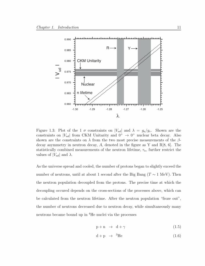
Figure 1.3: Plot of the 1 σ constraints on |Vud| and λ = ga/gv. Shown are theconstraints on |Vud| from CKM Unitarity and 0+ → 0+ nuclear beta decay. Alsoshown are the constraints on λ from the two most precise measurements of the β-decay asymmetry in neutron decay, A, denoted in the figure as Y and R[8, 6]. Thestatistically combined measurements of the neutron lifetime, τn, further restrict thevalues of |Vud| and λ.
As the universe spread and cooled, the number of protons began to slightly exceed the
number of neutrons, until at about 1 second after the Big Bang (T ∼ 1 MeV). Then
the neutron population decoupled from the protons. The precise time at which the
decoupling occured depends on the cross-sections of the processes above, which can
be calculated from the neutron lifetime. After the neutron population “froze out”,
the number of neutrons decreased due to neutron decay, while simultaneously many
neutrons became bound up in 4He nuclei via the processes
p + n → d + γ (1.5)
d + p → 3He (1.6)

Chapter 1. Introduction 12
3He + n → 4He (1.7)
These reactions continued for about three minutes and then essentially stopped be-
cause of the rapidly dropping temperature, density, and neutron population. Because
the neutron lifetime enters twice in the calculation of the 4He abundance (once in
determining the initial neutron population, then again as a process competing with
4He production), the measurement of the neutron lifetime is of great importance in
testing the Big Bang model of nucleosynthesis. About a quarter of the baryonic mat-
ter in the early universe is 4He, and the dominant uncertainty in the calculation of
the 4He/1H ratio is in the decay lifetime of the neutron[2].
The isotopic ratios predicted by BBN can be tested by observations of interstellar
gas clouds, where the abundances of light elements remain unchanged since the first
few minutes of the universe. Along with the cosmic microwave background, the
abundances of light elements are key predictions of the Big Bang theory. Accurate
knowledge of the neutron lifetime is critical in the interpretation of these data.
1.3 Previous experiments
The currently accepted value of the neutron lifetime is 885.7±0.8 s[5]. The uncertainty
in τn has dropped considerably in recent years, largely due to the establishment of
techniques involving UCN. Table 1.4 and Figure 1.4 summarize this recent progress.
Neutron lifetime experiments to date can be divided into two categories: those that
count neutron decays within a carefully defined beam volume, and those that count
the neutrons remaining within a confinement apparatus after a variable time. These
two methods suffer from quite different systematic uncertainties and thus complement
each other nicely. A third method, counting neutrons as they decay within a superfluid

Chapter 1. Introduction 13
Table 1.4: A summary of previous measurements of the neutron lifetime. Measure-ments with uncertainties greater than 10 s are not included.
Measured lifetime (s) Authors Method Reference
885.7 ± 0.9 ± 0.4 Arzumonov 00 UCN double bottle [13]
889.2 ± 3.0 ± 3.8 Byrne 96 Beam, Penning trap [14]
882.6 ± 2.7 Mampe 93 Material confinement, fomblin oil [15]
888.4 ± 3.1 ± 1.1 Nesvizhevsky 92 Material confinement [16]
887.6 ± 3.0 Mampe 89 Material confinement, fomblin oil [17]
891 ± 9 Spivak 88 Beam [18]
877 ± 10 Paul 89 Magnetic storage ring [19]
helium-filled magnetic trap, is the subject of this thesis, and has its own (albeit much
reduced) set of systematic uncertainties.
Beam method
In the beam method, neutron decays are counted within a carefully defined neutron
beam volume. The rate Cd of decay products emitted from a beam of known flux is
Cd = −dN
dt=
N
τ
where N is the average number of neutrons in the decay volume. Clearly several
quantities must be known quite accurately: the beam flux, the volume of beam ac-
cessible to the detectors, and the efficiency of detection. The most accurate mea-
surement to date using this method was performed by Byrne et al., finding a lifetime
of 889.2 ± 3.0 ± 3.8 s. In this experiment, the protons emitted in neutron decay
were captured in a Penning trap, then released periodically onto a detector. This

Chapter 1. Introduction 14
900
895
890
885
880
875
870
865
Mea
sure
d ne
utro
n lif
etim
e (s
)
200220001998199619941992199019881986
Year
Beam Material Confinement Magnetic Confinement
Figure 1.4: Previous measurements of the neutron lifetime. Three basic techniques areshown: beam, material storage, and magnetic storage. The horizontal line indicatesthe accepted (PDG) value, 885.7 ± 0.8 s. Error bars shown are the linear sum of thestatistical and systematic errors.
store-and-dump method allowed a high signal-to-noise ratio; almost all of the counts
detected were due to neutron decay. Experiments using the beam method are an
important check on measurements of the neutron lifetime using UCN storage, though
the formidable systematic uncertainties inherent to the beam method have prevented
comparable accuracy; at this time the most accurate measurements of the neutron
lifetime use UCN storage.
Storage Method
In the various storage methods, neutrons are contained within an apparatus for some
time, then counted. In this case, the number of neutrons in the apparatus is described

Chapter 1. Introduction 15
Li6
Figure 1.5: Schematic of the apparatus used in the beam lifetime measurement inreference [20]. A 10B target and α-detectors measure the beam flux, while decayprotons are stored in an electromagnetic Penning trap and then counted.
by
N(t) = N(0)e−t/τeff(t)
where
1
τeff=
1
τn+
1
τloss(t).
For all of these experiments there is some loss of neutrons from the apparatus; the
key is to understand and minimize these losses. However, N(0) need not be known
well; it must only be constant from run to run. In addition, the detection efficiency
need not be known well; it also must only be constant from run to run. It is possible
that τloss depends on time through an energy dependence; higher energy neutrons
may be more easily lost from the apparatus. In this case the time dependence of the
neutron population may be non-exponential.
One version of neutron storage was performed using an sextupole magnetic storage
ring. A conceptual drawing of this apparatus is shown in Figure 1.6. Neutrons were
loaded into the ring by moving the end of a neutron guide for a very short time into
the confinement region. Neutrons then orbited within the storage ring until a 3He
counter was placed in the beam. By varying the time at which the remaining neutrons

Chapter 1. Introduction 16
were counted, the lifetime of neutrons in the storage ring could be measured.
Because the stored neutrons were not energetically forbidden from leaving the
storage ring, the difficulty of estimating losses was the major uncertainty in this
experiment. Neutrons could be confined in semi-stable orbits, then be lost as transla-
tional momentum was transferred to transverse orbital oscillations; these are known
as betatron oscillations. Though most neutrons in semi-stable orbits were lost at
early times, betatron oscillations could in principle contribute to neutron losses, re-
sulting in a systematic uncertainty in the measurement of the neutron lifetime. The
measured neutron beta-decay lifetime in this experiment, 877 ± 10 s, is somewhat
shorter than the current accepted lifetime, but constitutes a strict lower limit on the
neutron lifetime.
Figure 1.6: A sketch of the idea of the NESTOR experiment.
The most successful measurements of the neutron lifetime have used material
confinement of UCN. In these experiments, a population of UCN are introduced
into a closed container and then counted some time later. A conceptual drawing of

Chapter 1. Introduction 17
this sort experiment is shown in Figure 1.7. Table 1.5 lists the Fermi potentials for
many different wall materials that can be used to store UCN. But more important
than a high Fermi potential is the need for a low neutron loss rate per bounce.
The two most successful approaches have used Fomblin oil and solid oxygen; both
of these surfaces exhibit very low UCN loss rates. In these experiments, UCN are
energetically forbidden from leaving the apparatus; however there is some loss due to
UCN upscattering from the surfaces, and this loss can depend on energy, yielding a
raw loss rate that is slightly non-exponential.
This loss is described by
< τ−1wall >=< µ(v)v > /λ
where µ(v) is the probability of loss per bounce, v is the velocity, <> represents the
average over the velocity spectrum, and λ the mean free path, as in kinetic theory
λ =4V
S
where S is the surface area of the storage vessel and V is the volume. The loss
probability is given by
µ(v) = 2f(arcsin(y)/y2 −√
(1 − y2)/y)
where y = v/vcrit (vcrit is the maximum velocity of the storable UCN as determined
by the Fermi potential and f is the ratio of the real to the imaginary parts of the
wall potential)[1].
Several approaches may be taken to understand spurious losses. One method is to
vary the S/V ratio in the experiment; by extrapolating to infinite volume the lifetime
may be extracted. Another method is to vary the energy spectrum of neutrons in the
bottle. One clever way to do this is to confine the UCN vertically using only gravity,

Chapter 1. Introduction 18
Table 1.5: UCN potentials for a variety of materials. This table is adapted largelyfrom references[1] and [21].
Material N a Vmat
(cm−3 × 10²²) (fm) (neV)
Ni58 9.0 14.4 346
BeO 7.25 13.6 257
Ni 9.0 10.6 252
Be 12.3 7.75 244
Diamond-like carbon 12.8 6.65 220
Stainless steel 8.5 8.6 188
Deuterated polystyrene 0.62 106.6 170
Cu 8.93 7.6 168
D2O 3.04 19.1 150
PTFE (Teflon) 2.65 17.6 124
Fomblin oil 0.043 956 106
Quartz 2.2 16.1 91
O2 2.68 11.6 80
Al 6.02 3.45 54
Chapter 1. Introduction 19
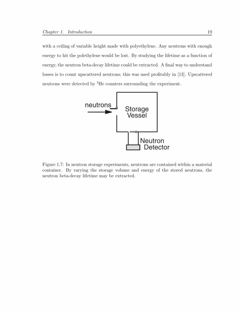
with a ceiling of variable height made with polyethylene. Any neutrons with enough
energy to hit the polethylene would be lost. By studying the lifetime as a function of
energy, the neutron beta-decay lifetime could be extracted. A final way to understand
losses is to count upscattered neutrons; this was used profitably in [13]. Upscattered
neutrons were detected by 3He counters surrounding the experiment.
neutrons
Neutron Detector
VesselStorage
Figure 1.7: In neutron storage experiments, neutrons are contained within a materialcontainer. By varying the storage volume and energy of the stored neutrons, theneutron beta-decay lifetime may be extracted.

Chapter 1. Introduction 20
1.4 Magnetic Trapping of Neutrons to Measure
the Neutron Lifetime
In neutron lifetime experiments using material storage, accuracy is limited by the
ability to stably control the number of stored neutrons from run to run, control
detection efficiency from run to run, and accurately extract τloss. In 1994, Doyle and
Lamoreaux published an idea for measuring the neutron lifetime that eliminates all of
these sources of systematic error[22]. In this method, UCN are magnetically trapped
within superfluid helium, and their decays are detected continuously by counting
pulses of scintillation light from the helium. Because the neutrons are energetically
forbidden from escaping from the trap and never touch a material wall, spurious losses
can be eliminated. And because the UCN are detected as they decay, variations from
run to run in the number of confined neutrons or detection efficiency do not contribute
to any systematic uncertainty.
Magnetic Trapping
To say that a particle is “trapped” means that its location is maintained within a given
region of space, and it is prevented from touching any physical walls. The last two
decades have seen enormous progress in trapping atoms, molecules, and fundamental
particles. Trapping allows particles to be probed with long interaction times and can
also permit a sample of particles to be thermally disconnected from the outside world.
Recent advances in atomic cooling are particularly striking, and depend on the newly
developed trapping technology.
One particularly popular sort of trap is the magnetic trap. This sort of trapping
field interacts with the magnetic moment of the trapped particle and can thus trap

Chapter 1. Introduction 21
electrically neutral species. As the magnetic moment of a given particle can be posi-
tive or negative depending on its spin state, a given particle can either be attracted
to higher or lower magnetic fields. It is not possible to create a magnetic field max-
imum in free space, but it is possible to create a magnetic field minimum[23]. Low
energy particles that are attracted to a lower magnetic field will orbit around the field
minimum.
Neutrons do not have a charge, so trapping must be achieved using their magnetic
moment. They interact with a magnetic field, �B, by the dipole interaction:
H = −�µ · �B
Because their magnetic moment is so small, neutrons must have very low energy
(∼ 1 mK) to be trapped. In the semi-classical picture, they precess around the
magnetic field with a frequency ω = 2µnB/� (or ω2π
≈ 29 MHz at 1 Tesla). If the
precession frequency is much higher than the change in the magnetic field seen by the
neutron,
2µnB
�� d �B/dt
| �B|,
then the magnetic moment of the neutron will follow the direction of the field adia-
batically. Then the trap depth depends only on the magnitude of the magnetic field,
not its direction.
One common magnetic field configuration is known as the Ioffe trap. The currents
in an Ioffe trap are depicted in Figure 1.8. The four current bars create a field that
rises in magnitude with radius, while the two current loops of the same sense provide
axial confinement. This trap configuration has no point at which the magnitude of
the magnetic field is zero. Therefore trapped particles precess with a high enough
frequency that they do not flip their spin. The trap volume is roughly cylindrical. A
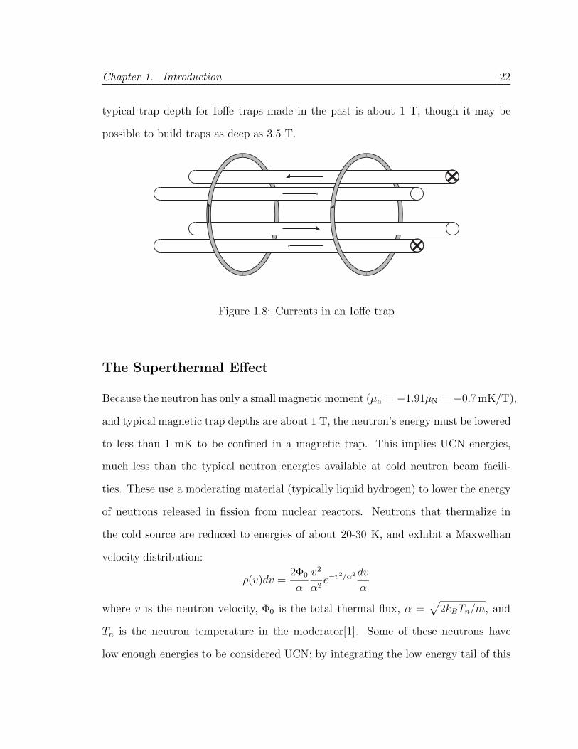
Chapter 1. Introduction 22
typical trap depth for Ioffe traps made in the past is about 1 T, though it may be
possible to build traps as deep as 3.5 T.
Figure 1.8: Currents in an Ioffe trap
The Superthermal Effect
Because the neutron has only a small magnetic moment (µn = −1.91µN = −0.7mK/T),
and typical magnetic trap depths are about 1 T, the neutron’s energy must be lowered
to less than 1 mK to be confined in a magnetic trap. This implies UCN energies,
much less than the typical neutron energies available at cold neutron beam facili-
ties. These use a moderating material (typically liquid hydrogen) to lower the energy
of neutrons released in fission from nuclear reactors. Neutrons that thermalize in
the cold source are reduced to energies of about 20-30 K, and exhibit a Maxwellian
velocity distribution:
ρ(v)dv =2Φ0
α
v2
α2e−v2/α2 dv
α
where v is the neutron velocity, Φ0 is the total thermal flux, α =√
2kBTn/m, and
Tn is the neutron temperature in the moderator[1]. Some of these neutrons have
low enough energies to be considered UCN; by integrating the low energy tail of this

Chapter 1. Introduction 23
distribution one finds:
ρUCN =2
3
Φ0
α
(EUCN
kBT)3/2
)
where EUCN is the maximum UCN energy. The maximum density of UCN that has
been achieved using this method is about 90 cm−3 at the Institut Laue-Langevin in
Grenoble, France.
Because these neutrons are in thermal equilibrium with the moderator, the rate
of UCN upscattering to high energies is equal to the rate of high energy neutrons
scattering to UCN energies. Consider the cross-section for neutrons scattering from
a state of energy ∆ to energy EUCN . Detailed balance then implies:
EUCN
kBTe−EUCN/kBTσ(EUCN → EUCN + ∆) = (1.8)
EUCN + ∆
kBTe−(EUCN+∆)/kBT σ(EUCN + ∆ → EUCN )
which we can then write as an expression for the upscattering rate:
σ(EUCN → EUCN + ∆) =EUCN + ∆
EUCNe−∆/kBTσ(EUCN + ∆ → EUCN). (1.9)
Note that the upscattering cross-section decreases exponentially with moderator tem-
perature. If the temperature is low, e.g. ∆ >> kBT >> EUCN , then the upscattering
rate can be made arbitrarily small.
This suppression of neutron upscattering allows the possibility of a second method
of producing UCN. If neutrons with energy ∆ have a resonance for scattering to
UCN energies, then the density of UCN will build up to a value proportional to
(EUCN/∆)e∆/kBT . The density thus increases exponentially as the temperature de-
creases instead of as 1/T 2 as found in a thermal moderator. The neutrons do not have
to come into thermal equilibrium with the moderator for this “superthermal process”
to proceed. Observe that in order for the superthermal process to produce a large
number of UCN, there must be a significant number of neutrons with energy ∆. If the
Chapter 1. Introduction 24
neutrons were at the moderator temperature T , then the flux of neutrons at energy
∆ would be down by a factor e−∆/kBT , thus canceling out the superthermal enhance-
ment. It can thus be seen that the superthermal effect requires a large temperature
difference between the neutron beam and the moderator to create a significant pop-
ulation of UCN. If the system is viewed thermodynamically as a neutron population
(A) and a moderator (B), then the entropy and phase space of (A) decrease while the
entropy and phase space of (B) and the system (A+B) both increase. The increase
in entropy and phase space of (B) is a result of the excitation of the moderator, and
allows the decrease of entropy and phase space of (A)[1].
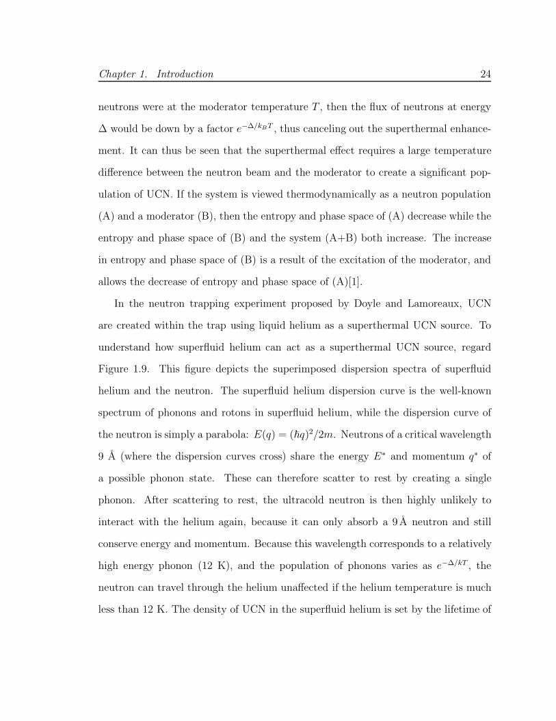
In the neutron trapping experiment proposed by Doyle and Lamoreaux, UCN
are created within the trap using liquid helium as a superthermal UCN source. To
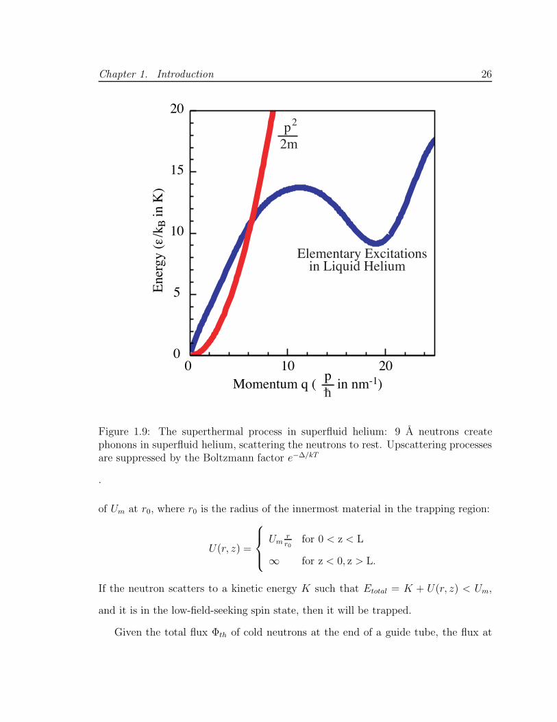
understand how superfluid helium can act as a superthermal UCN source, regard
Figure 1.9. This figure depicts the superimposed dispersion spectra of superfluid
helium and the neutron. The superfluid helium dispersion curve is the well-known
spectrum of phonons and rotons in superfluid helium, while the dispersion curve of
the neutron is simply a parabola: E(q) = (�q)2/2m. Neutrons of a critical wavelength
9 A (where the dispersion curves cross) share the energy E∗ and momentum q∗ of
a possible phonon state. These can therefore scatter to rest by creating a single
phonon. After scattering to rest, the ultracold neutron is then highly unlikely to
interact with the helium again, because it can only absorb a 9 A neutron and still
conserve energy and momentum. Because this wavelength corresponds to a relatively
high energy phonon (12 K), and the population of phonons varies as e−∆/kT , the
neutron can travel through the helium unaffected if the helium temperature is much
less than 12 K. The density of UCN in the superfluid helium is set by the lifetime of

Chapter 1. Introduction 25
the neutrons τ and the production rate P (Eu):
P (Eu)dEu = Φ(E∗)nσcohαS(q∗)√
Eu/E∗dEu
where α = |vn/(vn−vg)| and vg = ∂ω(q∗)/∂q, the phonon group velocity. P is equal to
the neutron flux at 9 A, multiplied by the scattering cross-section and integrated up to
the maximum UCN energy EUCN . The UCN density increases through superthermal
production, but decreases through neutron loss, that is:
dρu
dt= P − ρu/τ.
The solution of this differential equation is
ρu = Pτ (1 − e−t/τ),
which implies a maximum UCN density of Pτ .
The superthermal effect allows an enormous increase in phase space for the down-
scattered neutrons. The incident neutrons occupy a volume in k space of 8πk∗2kUCN
and the UCN occupy a volume of 43πk3
UCN , a boost in phase space density of 6(k∗/kUCN )2.
This is possible because the created phonons carry away the extra energy, and the en-
tropy of the helium bath increases more than the entropy of the neutrons decreases[24].
Loading the Trap
The mean free path for a 9 A neutron in superfluid helium is over 100 m. Therefore
the UCN production rate in the trap will be essentially uniform. Low-field-seeking
neutrons that scatter to an energy below the trap depth Um will be magnetically
trapped.
The trapping field can be approximated by a cylindrically symmetric potential,
with infinite potential for z < 0, z > l and rising linearly with radius to a maximum
Chapter 1. Introduction 26
0
5
10
15
20
0 10 20Momentum q ( in nm-1)
p2
2m
Elementary Excitationsin Liquid Helium
Ene
rgy
(ε/k
B in
K)
ph
Figure 1.9: The superthermal process in superfluid helium: 9 A neutrons createphonons in superfluid helium, scattering the neutrons to rest. Upscattering processesare suppressed by the Boltzmann factor e−∆/kT
.
of Um at r0, where r0 is the radius of the innermost material in the trapping region:
U(r, z) =
Umrr0
for 0 < z < L
∞ for z < 0, z > L.
If the neutron scatters to a kinetic energy K such that Etotal = K + U(r, z) < Um,
and it is in the low-field-seeking spin state, then it will be trapped.
Given the total flux Φth of cold neutrons at the end of a guide tube, the flux at

Chapter 1. Introduction 27
the critical energy E∗ can be found using
Φ(E∗) = ΦthE∗
T 2e−E∗/T ,
where T is the neutron temperature exiting the cold source. By integrating the
production rate P over trap volume and UCN energy , one can calculate the expected
number of trapped neutrons. Depending on the neutron flux, trap volume, and trap
depth, the number of trapped neutrons can vary between 103 and 105 per load. A
description of Monte Carlo simulations of neutron trapping may be found in reference
[25].
Detecting Trapped Neutrons
After the neutrons are accumulated in the trap for about half an hour, the beam is
shut off. Neutrons with energies above the trap depth are quickly absorbed, while
trapped neutrons spiral around the magnetic field minimum until they decay. When
this happens, the electron and antineutrino carry most of the decay energy. The
antineutrino leaves the experiment, while the electron deposits its energy within the
liquid helium. The helium then scintillates in the extreme ultraviolet (EUV). The
scintillation is highly efficient; about 35% of the energy of the recoiling electron is
converted into prompt scintillation light. For a electron carrying 250 keV of kinetic
energy, this corresponds to 5500 EUV photons. Unfortunately, EUV light cannot pass
through most materials, though it easily travels through liquid helium. Therefore the
walls of the trap are coated with a coating of fluor that converts the ultraviolet light
to visible blue light. The blue light then travels out of the apparatus through light
guides and is detected by light-sensitive photomultipliers at room temperature. The
detection of neutron decays using liquid helium as a scintillator is discussed in great
detail in Chapter 2.

Chapter 1. Introduction 28
liquid helium
2He *
e–
γ – 80nm
γ – 430nm
TPB
Figure 1.10: The principle behind the detection of neutron decay in superfluid helium.
Systematics
As mentioned above, this experiment should not suffer from many of the sources of
systematic error that affect other neutron lifetime experiments. Because the decay
curves observed can simply be added together and then fit, the experiment is not af-
fected in a systematic way by fluctuations in neutron beam flux or detection efficiency.
And because the neutrons do not interact with material walls, upscattering can be
minimized in a simple way. There are several other possible sources of systematic
error unique to this experiment, but all of these should be controllable at the 10−5
level.
The chance per second k that a given neutron will be absorbed by a 3He nucleus
is
k = σtvt
vHenvHe = σtvtn
where σt is the thermal neutron absorption cross-section on 3He, vt is the velocity of
a thermal neutron, vHe is the velocity of 3He nuclei in the liquid helium bath, and n
is the density of 3He nuclei. The factor vt/vHe takes into account the cross-section
enhancement at low relative velocity. Note that the temperature of the helium bath
is irrelevant, as the 3He velocity cancels out.
Chapter 1. Introduction 29
Expressed as an absorption lifetime τ , we have
τ =1
k=
1
σtvtn=
3.15 × 10⁻⁸
fs
where f is the 3He/4He ratio. By using helium with a 3He/4He of less than 3 × 10⁻¹⁵
one can suppress neutron absorption loss to 10−4 of the neutron beta-decay rate.
This can be done using a heat flush method, in which 3He nuclei are removed using
a phonon wind in superfluid helium[26].
It is possible that some neutrons might scatter to energies slightly above the trap
depth, yet not immediately impinge on the walls of the chamber. These neutrons
might suffer from losses other than beta decay, thus rendering the neutron decay
spectrum non-exponential and shortening the measured decay lifetime. This can
happen if the energy is shared by several modes of motion. For example, a neutron
with significant axial motion might slowly convert its kinetic energy to radial oscil-
lations, hit the walls, and be lost. In order to eliminate these marginally trapped
neutrons, one can temporarily lower the magnetic field, then raise it back. Calcula-
tions have shown that temprarily lowering the trapping field to 30% of its final value
should eliminate all marginally trapped neutrons, while throwing away 50% of the
trapped neutrons[23].
A second possible effect is a time-dependent detection efficiency due to an evolving
distribution of neutrons in the various oscillatory modes within the trap. Because the
electron emitted in beta decay can travel as far as 1 cm (a significant portion of the
trap radius) within the liquid helium, and any energy deposited in the walls is not
converted to EUV light, a slow movement of neutrons to larger radii would result in
a detection efficiency that was decreasing with time, systematically decreasing the
measured lifetime. This possible systematic would have to be studied by lowering
the trap depth temporarily to eliminate trapped neutrons with trajectories near the

Chapter 1. Introduction 30
cell walls. It is believed that the entropic mixing of trajectory modes is rapid; in this
case the detection efficiency should vary little with time over the neutron confinement
period.
It is possible for trapped neutrons to flip spin, dropping in potential energy into
a high-field seeking state. These neutrons would be immediately lost from the trap,
shortening the measured lifetime. This loss mechanism can however be easily min-
imized by ensuring that the magnetic field experienced by the trapped neutrons is
non-zero. Even a small magnetic field will ensure that the neutrons do not spin-flip;
calculations show that a bias field of 0.1 T should ensure that the trap loss due to
spin flips be less than 10−4 of the beta-decay rate[23].
Trapped UCN cannot be absorbed by the 4He because this process is energeti-
cally forbidden. However, the UCN can be affected by phonons in the superfluid. As
mentioned above, single-phonon absorption is highly suppressed because the temper-
ature of the helium bath is significantly less than the critical phonon temperature of
12 K. Phonons with this energy are very rare at low helium temperatures, and highly
unlikely to be absorbed by a trapped neutron. Instead, the dominant interaction of
a phonon with a trapped neutron is two-phonon scattering. The rate of two-phonon
scattering varies as T 7 where T is the temperature of the helium bath. At a temper-
ature of 150 mK, the UCN upscattering lifetime is 108 s, yielding a negligible effect
on the trapped neutron lifetime[23].
A final possible source of systematic error is neutron activation of materials sur-
rounding the trap. If elements such as Al, Cu, V, or Si are activated, they will decay
with lifetimes on the order of the neutron lifetime, releasing gamma rays, alphas,
or betas into the superfluid helium. These decays will compete with the decays of
trapped neutrons, creating a systematic uncertainty. This possibility requires careful

Chapter 1. Introduction 31
shielding of the neutron beam to avoid activation backgrounds.

Chapter 2
Scintillations in Liquid Helium:
History and Motivation
2.1 Historical Background
The fact that liquid helium scintillates was established in 1959 by Thorndike and
Shlaer[27] and simultaneously by Fleishman, Einbinder and Wu [28]. From their
experiments, it was clear that helium emits light in the far ultraviolet when excited
by ionizing radiation. The scintillation could be detected by coating the walls of the
helium bath with an organic fluor, which would shift the wavelength of the scintillation
light to the visible and render it detectable via a photomultiplier tube. Further
experiments showed the scintillation pulse to be very fast, with a decay time of less
than 10 ns[29]. The light did not pass through any standard window materials, even
ones with very low cutoff wavelengths such as LiF[30]. Studying the scintillation
pulses more carefully, Moss and Hereford found that the scintillation intensity from
α sources had a peculiar temperature dependence below the λ point[31], and Kane
et al. showed that beta sources did not display the same behavior. Based on this
32

Chapter 2. Scintillations in Liquid Helium: History and Motivation 33
observation, Hereford and Moss speculated that the scintillation could come from
excited atoms or metastable states of the liquid[32]. Later, Jortner et al. showed
that impurities suspended in the helium fluoresced in the visible, suggesting energy
transfer from a helium metastable state[33]. But it was almost a decade before the
scintillation mechanism was understood.
Meanwhile, liquid helium was under intense investigation for its fascinating super-
fluid properties. Its low energy excitations (phonons, rotons, and vortices) were a rich
source of information about the superfluid state, and the subject of much experimen-
tation. Then, in 1968, Surko and Reif discovered a new, fourth, kind of long-lived
neutral excitation[34]. By immersing an alpha source (210Po) in cold (T < 0.6 K)
superfluid helium, excitations were produced that could travel through the liquid for
distances greater than 1 cm without appreciable scattering or attenuation, causing
He+ ions and electrons to be emitted from the surface of the liquid helium, or positive
ions and electrons to be emitted from a metal plate placed in the liquid. Because
the excitations could ionize helium atoms (Ei = 24.6 eV), they clearly were much
more energetic than phonons, rotons, and vortices; however the nature of these new
neutral excitations was unknown. Later work showed that there was a substantial
delay between the creation of the excitations and their arrival at the surface, and that
beta excitation could also produce them[35, 36].
Then a breakthrough experiment gave reason to believe that the unknown source
of EUV light and the unknown neutral excitation were both excited helium electronic
states. In 1969, Dennis et al. measured the visible and near-infrared light spec-
trum from liquid helium bombarded by an intense 160 keV electron beam and found
emission from both helium atoms and diatomic helium molecules[37]. In particular,
it was shown that the molecular singlet and triplet ground states, He2(A1Σ+
u ) and

Chapter 2. Scintillations in Liquid Helium: History and Motivation 34
He∗2(a
3Σ+u ), were populated at a rapid pace. Both of these molecules are unstable for
radiative decay to two ground state helium atoms and both emit a ∼ 16 eV (80 nm)
photon when they decay. However their radiative lifetimes are much different. The
He2(A1Σ+
u ) molecule decays in less than 10 ns, whereas the radiative lifetime of the
He∗2(a
3Σ+u ) molecule is on the order of 10 seconds, since the decay to two helium atoms
requires an electron spin flip[38]. The He∗2(a
3Σ+u ) molecule was thus a plausible can-
didate for the neutral excitation discovered by Surko and Reif, while the He2(A1Σ+
u )
was the source of scintillation pulses.
Additional interesting measurements were made possible by studying the transient
behavior of individual atomic and molecular emission bands. If the electron beam
were suddenly turned off at time t = 0, then the density of He∗2(a
3Σ+u ) molecules
was seen to decay rapidly, with a 1/t dependence[39, 40, 41]. This behavior could
be explained by the hypothesis that He∗2(a
3Σ+u ) molecules react with each other by
Penning ionization:
He∗2 + He∗
2 → 3He + He+ + e−
or
He∗2 + He∗
2 → 2He + He+2 + e−.
Penning ionization can happen because two excited helium molecules together have
enough internal energy to ionize a helium atom. It requires no activation energy and
occurs with nearly unity probability if the molecules collide. Penning ionization is
a two-body reaction; this implies that the concentration M of metastable molecules
is described by the equation dM/dt = −α(T )M2, which has the solution 1/M =
1/M0 + α(T )t), where α(T ) is the bilinear reaction coefficient and M0 is the initial
concentration of He∗2(a
3Σ+u ) molecules. The reaction coefficient α(T ) was measured to
be about 109 cm3 s−1, and decreased with increasing temperature, indicating that the

Chapter 2. Scintillations in Liquid Helium: History and Motivation 35
reaction rate is affected by the roton density in the liquid. The higher the temperature,
the higher the roton density, and the longer it takes two molecules to diffuse through
the roton gas, find each other, and react.
It was also found that metastable He(23S) atoms are created in copious numbers
as a result of the electron beam. But though this atom has an 8000 s radiative
lifetime in vacuum[42], it does not last long in the helium liquid. The He∗(23S)
density was found to drop exponentially, with a 15 µs lifetime. A concurrent rise in
density of vibrationally excited He∗2(a
3Σ+u ) molecules was also seen, lending evidence
to the hypothesis that in the dense liquid helium environment, ground state helium
atoms can tunnel into the (23S) potential, forming vibrationally excited He∗2(a
3Σ+u )
molecules. This reaction does not happen instantaneously because there is a 60 meV
potential barrier between the He(23S and He(11S atoms[43]. This potential barrier
is lowered at high densities, indicating that a third helium atom can lower the barrier
significantly.
Further work centered on measuring the extreme ultraviolet scintillation spectrum
using a grated EUV spectrometer[44, 45, 46]. It was found that a very intense con-
tinuum was produced in the wavelength range from 60 to 100 nm, corresponding to
the reaction
He2(A1Σ+
u ) → 2He(11S) + �ν.
The EUV spectrum measured in reference [44] is shown in Figure 2.1. The large
wavelength spread is a consequence of the fact that the reaction product (two free he-
lium atoms) is not a bound state. In the Oppenheimer approximation, the slowly mov-
ing helium nuclei do not change position during a fast electronic transition. Therefore
the amount of energy released as light depends on the distance between the two He
nuclei at the time of radiative decay. The remaining energy goes into kinetic energy

Chapter 2. Scintillations in Liquid Helium: History and Motivation 36
of the two final 11S helium atoms.
Figure 2.1: The scintillation spectrum of electron-bombarded liquid helium (fromreference [44].
The bands at the short wavelength end of the spectrum are believed to be due
to the radiative decay of high vibrational states of He∗2(A
1Σ+u ). The high vibra-
tional levels are probably populated in a similar way as the high vibrational levels
of He∗2(a
3Σ+u ): reactions of excited helium atoms with the surrounding helium. Just
as He∗(23S) atoms react with surrounding helium atoms to form vibrationally ex-
cited He2(a3Σ+
u ), He(21S) atoms react with the liquid to form vibrationally excited
He2(A1Σ+
u ). The time for this process to occur has not been measured, but should
be comparable to the 15 µs lifetime of the He∗(23S) atom.
It was also found that varying the location of the electron beam relative to the
liquid helium surface had little effect on the measured EUV intensity. The scintillation
light was unattenuated by as much as 10 cm of liquid helium. The transparency of

Chapter 2. Scintillations in Liquid Helium: History and Motivation 37
25
20
15
10
5
0
Ene
rgy
(eV
)
3. 02.52.01.51.00.50.0Interatomic distance (Angstroms)
λ = 60 - 100 nm
X1Σ+g
A1Σ+u
11S + 11S
21S + 11S
Figure 2.2: The potential curves of He2(A1Σ+
u ) and the ground state He2(X1Σ+
g )(equivalent to two free He atoms).
liquid helium to its own scintillation light can be explained by the high energy needed
to excite atomic helium; the difference in energy between the 11S ground state and
the first atomic helium excited state is 20 eV, more energy than that of the 16
eV photons emitted in helium excimer decay. The fact that singlet production is
enhanced in the liquid, plus the fact that helium does not absorb its own scintillation
light, results in an extremely bright EUV pulse from He2(A1Σ+
u ) decay. In fact,
the ultraviolet emission accounts for over 99% of the total scintillation intensity[44].
The extraordinary intensity of the ultraviolet emission has been measured recently
by Adams et al.; they find that 35% of the energy deposited by beta particles in
superfluid helium is emitted as prompt EUV light[47, 48].
Because the He∗2(a
3Σ+u ) molecules are destroyed by Penning ionization in these
experiments, the spectrum was dominated by He2(A1Σ+
u ), which can radiatively de-

Chapter 2. Scintillations in Liquid Helium: History and Motivation 38
cay before reacting with other metastables[40, 41]. But while triplet molecules were
destroyed quickly in the spectroscopic measurements that required high molecular
densities, they can survive for very long times (∼ 10 s) in experiments where the ex-
citation was more modest (such as the Surko and Reif experiment). If the excitation
density were lower, then one might expect to see contributions from He∗2(a
3Σ+u ) decay
as well.
Such experiments using weak radioactive sources were carried out in parallel by
the Hereford group at the University of Virginia. But instead of looking at atomic
and molecular spectra, these experiments used a wavelength shifting fluor deposited
on the cavity walls to convert the EUV scintillation light to the visible. This had
the drawback of not being able to discriminate different atomic and molecular states,
but allowed the study of individual decay events. Several interesting results followed
from this work. First, it was found that the intensity of scintillation pulses created
using an alpha source decreased significantly as the helium was cooled; as mentioned
above, this was one of the first pieces of evidence for the creation of metastable
excited states in the liquid helium. Second, it was shown that the scintillation light
could be significantly quenched by the application of an electric field. By studying
how the pulse height varied with electric field strength, and estimating the number
of ion-electron pairs produced, they estimated that 60% of the scintillation pulse
intensity derives from electron-ion recombination. Third, it was found that excited
liquid helium emits a large number of photons well after the initial scintillation pulse.
The rate of delayed photons depended on both temperature and the size of the helium
bath, suggesting that the photons were emitted by metastables that diffused through
the liquid helium and were quenched when they hit the wall.
Work in more recent decades has centered on the study of the metastable molecule
Chapter 2. Scintillations in Liquid Helium: History and Motivation 39
He∗2(a
3Σ+u ). It was found that these molecules in solid helium decay radiatively with
a lifetime of about 15 s[49]. This long lifetime could be observed spectroscopically
in this case since Penning ionization in the solid was suppressed by slow molecular
diffusion. Later attempts to suppress Penning ionization in the liquid by application
of a strong magnetic field proved unsuccessful[50]. Another group managed to set a
lower limit of 10 seconds on the He∗2(a
3Σ+u ) lifetime in liquid helium by measuring the
time of flight between a discharge and a surface ionization detector[51].
2.2 Fundamental Physics Experiments Using
Liquid Helium as a Scintillator
In recent years, the application of liquid helium as a scintillator has received new
attention. Possible experiments that would make use of the large scintillation yield of
liquid helium are the search for the neutron electric dipole moment, the measurement
of the neutron beta-decay lifetime, and the detection of low energy solar neutrinos.
In the search for the electric dipole moment (EDM) of the neutron, a method
recently proposed by Golub and Lamoreaux promises significant gains in sensitivity.
In this approach, ultracold neutrons are produced in superfluid helium doped with
polarized 3He[52]. The neutron absorption cross-section of 3He is strongly dependent
on the relative spin of the neutron and 3He nucleus. By giving the neutrons and
3He nuclei each a π/2 spin flip, the difference between the precession frequency of
the neutron and that of the 3He nucleus can be measured by monitoring the rate
of 3He(n, p)3H events detected by counting pulses of EUV scintillation light. By al-
ternating the direction of a strong electric field (either parallel or antiparallel to the
magnetic field), and looking for a change in the scintillation rate, several orders of
Chapter 2. Scintillations in Liquid Helium: History and Motivation 40
magnitude more sensitivity for the neutron electric dipole moment may be obtained.
The gains in sensitivity derive from the high density of UCN produced in the su-
perthermal process and the high electric field that can be tolerated in liquid helium.
This experiment requires tight control over stray magnetic fields, and must be sur-
rounded by mutiple layers of magnetic shielding. This places constraints on the type
of light collection system used to detect helium scintillation events. The detector will
have to be carefully designed, and may make use of wavelength shifting fibers, as this
will allow the scintillation signal to be passed out of the cryogenic region without
seriously compromising the limits on magnetic field inhomogeneities. However, the
signal yield from fiber-based detectors is not high, and in addition the scintillation
signal will be significantly decreased by the application of the electric field, since
most of the signal from the main pulse is a result of ion-electron recombination[53].
Detector designs based on wavelength shifting fibers will be discussed in Chapter 3.
The detectors described in the next chapter were designed specifically for the mon-
itoring of decays of ultracold neutrons in a superfluid helium-filled magnetic trap. In
this experiment, first proposed by Doyle and Lamoreaux in 1994, neutrons are loaded
into the trap through inelastic scattering in superfluid helium, and then the same
helium is used as a scintillator to detect their decay[22]. Because of the spectre of
neutron activation, the design of these detectors was constrained significantly; the
only elements allowed in the materials used to construct the detectors were car-
bon, hydrogen, oxygen, fluorine, and boron. Initially, an additional constraint was
imposed: that the neutron beam be allowed to pass through the detector without
significant absorption. This constraint was later removed, and allowed more efficient
scintillation detection. The program of detector development was begun in 1995, and
is the primary subject of the next chapter.

Chapter 2. Scintillations in Liquid Helium: History and Motivation 41
Superfluid helium has also been suggested as a medium for detecting the elastic
scattering of low energy solar neutrinos. Because superfluid helium can be easily
cleaned of radioactive impurities, it is a promising medium for this low-background
experiment. Two distinct approaches to capturing the scintillation signal have been
proposed, one using silicon calorimeters[54] (HERON), and one using wavelength
shifters and photomultipliers (CLEAN). The two approaches do not only differ in the
technology used to detect EUV scintillation, but also employ very different approaches
to background rejection. The CLEAN approach was inspired largely by the neutron
beta-decay detector development program described in the next chapter, but a full
explanation of the CLEAN approach is beyond the scope of this thesis. For those
that are interested, the CLEAN method is described in reference [55].
Chapter 3
Detector Development
In recent years, superfluid helium has come under increased scrutiny as a scintillation
medium for detecting ionizing radiation. While quite low temperatures are neces-
sary to liquify helium, and therefore experimental conditions are more difficult than
with more conventional scintillators, certain experiments in fundamental physics can
take advantage of superfluid helium’s special characteristics (such as zero neutron
absorption and low thermal excitation density) while simultaneously making use of
its scintillation properties.
The scintillation from ionizing radiation events in liquid helium can divided into
three parts: a prompt component, an afterpulsing component, and a phosphorescence
component. These three processes are manifested on radically different time scales
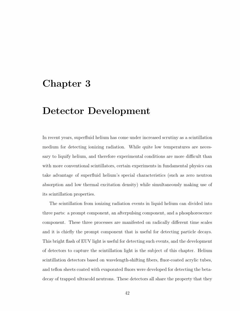
and it is chiefly the prompt component that is useful for detecting particle decays.
This bright flash of EUV light is useful for detecting such events, and the development
of detectors to capture the scintillation light is the subject of this chapter. Helium
scintillation detectors based on wavelength-shifting fibers, fluor-coated acrylic tubes,
and teflon sheets coated with evaporated fluors were developed for detecting the beta-
decay of trapped ultracold neutrons. These detectors all share the property that they
42

Chapter 3. Detector Development 43
use wavelength shifting fluors to convert the EUV scintillation light to visible light,
which can then be transported out of the cryogenic apparatus to detectors at room
temperature.
3.1 Fluor Development
Detector development for the neutron trapping experiment began with a measurement
of the EUV yield of several fluorescent materials. These materials emit visible light
upon the absorption of EUV radiation. Direct EUV detection, although possible
with high efficiency, can be problematic due to the inability to transmit or guide EUV
radiation to a detector; use of wavelength shifters alleviates this problem. In addition,
wavelength shifting can significantly increase the number of photons available for
detection.
The EUV scintillators tetraphenyl butadiene (TPB), p-terphenyl (TPH), and
diphenyl stilbene (DPS) have emission spectra with peaks at 440 nm, 335 nm, and
409 nm respectively, each with widths of about 50 nm. They are all well suited for en-
ergy downconversion because of their high fluorescence efficiencies[56, 57, 58, 59, 60]
and they can be evaporated into thin films, yielding adherent, durable coatings. The
chemical composition of one of these fluors (TPB) is shown in Figure 3.1. In contrast
to these evaporated films, fluor doped plastic films have the advantages of less light
scattering, better abrasion resistance, ease of preparation, and index matching to
plastic light guides[61]. These qualities have led to the consideration of using doped
plastic films in several applications, including detection of Cerenkov radiation[62],
ultraviolet imaging[63], and detection of dark matter[56]. However, fluorescence effi-
ciencies of doped plastic films have been measured to be lower than their evaporated
film counterparts at short wavelengths[56, 63].
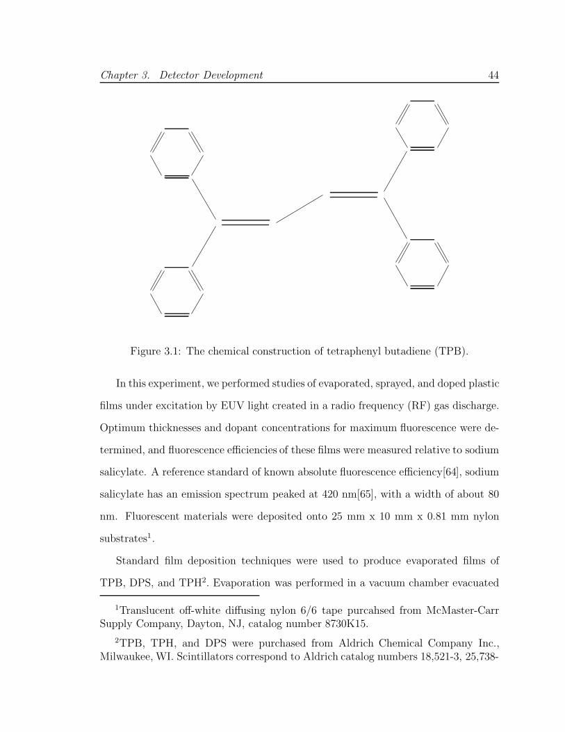
Chapter 3. Detector Development 44
Figure 3.1: The chemical construction of tetraphenyl butadiene (TPB).
In this experiment, we performed studies of evaporated, sprayed, and doped plastic
films under excitation by EUV light created in a radio frequency (RF) gas discharge.
Optimum thicknesses and dopant concentrations for maximum fluorescence were de-
termined, and fluorescence efficiencies of these films were measured relative to sodium
salicylate. A reference standard of known absolute fluorescence efficiency[64], sodium
salicylate has an emission spectrum peaked at 420 nm[65], with a width of about 80
nm. Fluorescent materials were deposited onto 25 mm x 10 mm x 0.81 mm nylon
substrates1.
Standard film deposition techniques were used to produce evaporated films of
TPB, DPS, and TPH2. Evaporation was performed in a vacuum chamber evacuated
1Translucent off-white diffusing nylon 6/6 tape purcahsed from McMaster-CarrSupply Company, Dayton, NJ, catalog number 8730K15.
2TPB, TPH, and DPS were purchased from Aldrich Chemical Company Inc.,Milwaukee, WI. Scintillators correspond to Aldrich catalog numbers 18,521-3, 25,738-
Chapter 3. Detector Development 45
using a diffusion pump with a liquid nitrogen cooled baffle to less than 10−5 mbar.
Film thickness was controlled by varying the distance from the molybdenum evap-
oration boat to the film substrate. Sample thickness is measured by weight, and
ranges from 49 ± 6 µg cm−2 to 2650 ± 100 µg cm−2, with uncertainties in thickness
determined by the uncertainty in the weighing technique.
Sprayed phosphor coatings of sodium salicylate and TPB were prepared by air-
brushing scintillator solution onto nylon substrates3. The scintillator solution con-
sisted of either sodium salicylate dissolved in methyl alcohol or TPB dissolved in
ethyl ether. Though easier to prepare, films made using this technique are less uni-
form than evaporated films. Film thickness was measured by weight, and ranged from
80 ± 40 µg cm−2 to 3040 ± 40 µg cm−2.
Doped plastic films used in the EUV discharge source measurements were pre-
pared by either a) controlled dipping of the substrate into a solution of the plastic
and dopant, b) dripping the solution directly onto the substrate, or c) spinning plastic-
dopant solution onto the substrate using a commercial spinner. In cases a) and b) the
solutions consisted of 30 ml toluene per gram of plastic, with a varying concentration
of fluor. Film thickness was measured using a micrometer. Dipped films are 12 ±
2 µm thick, while the films formed by dripping are 31 ± 2 µm thick. Chloroform is
used as a solvent in the making of the spun films. Thicknesses of spun films (case c)
range from 1.6 ± 0.1 µm to 40.1 ± 0.1 µm, as measured with a profilometer. The
plastic used for most applications was pure polystyrene, with an average molecular
weight of 280,000. Also tested are polyvinyltoluene (PVT), poly(2,4-dimethylstyrene)
9, and D21,375-6.
3Airbrush model CCAKCC, Paasche Airbrush Co., Harwood Heights, IL.

Chapter 3. Detector Development 46
(PDMS)4, polymethylmethacrylate (PMMA), nitrocellulose5, long chain polystyrene
(M.W. = 1,880,000), short chain polystyrene (M.W. = 2727), and dicarboxy termi-
nated polystyrene6.
PMT
Quartz discharge tube
RF coil
Al XUVwindow
Sample
Glass window
Gas
To pump
Figure 3.2: Apparatus used to measure fluorescence efficiencies of thin film samples.
Fluorescence efficiency measurements were performed by illuminating thin film
samples with EUV light and measuring the intensity of the emitted fluorescent light
with a photomultiplier tube (See Figure 3.2). The EUV source was a 66 MHz RF
discharge in 99.999% pure helium (58.4 nm) or 99.995% pure neon (74.0 nm) gas.
A continuous flow of gas through the system was required to maintain cleanliness.
We found this to be important for maintaining a high EUV intensity. Visible and
near UV light is filtered from the excitation spectrum by a 200 nm thick aluminum
window[65]. The filtered spectrum consists solely of the desired EUV line. This
was verified by measuring the output spectrum of the EUV system with a vacuum
4PDMS provided by Dr. R. G. Jones, Centre for Materials Research, Universityof Kent at Canterbury.
5Nitrocellulose was purchased from Ernest J. Fullam, Inc., Latham, N. Y., catalognumber 11282.
6With the exception of PDMS and nitrocellulose, all plastic resins were purchasedfrom Aldrich Chemical Company Inc., Milwaukee, WI. Plastics correspond to Aldrichcatalog numbers 18,242-7, 18,282-6, 18,224-9, 32,781-6, 32,771-9, and 18,961-8.
Chapter 3. Detector Development 47
ultraviolet spectrometer7.
Twenty-one samples could be loaded into the apparatus at one time and could
be interchanged and tested in situ. The EUV light emitted from the RF discharge
illuminated a central area of 5 mm2 on an individual sample. Scintillation light that
entered into the diffusing nylon substrate has its direction randomized. This ensured
that for a constant geometry, a fixed portion of light was collected by the bialkali
cathode photo-multiplier tube (PMT) positioned directly behind the sample. The
PMT was biased within the linear range of its voltage divider circuit. Comparison
of the recorded anode currents, corrected for the wavelength dependent photocath-
ode sensitivity, determined the relative fluorescence efficiencies of the samples. No
fluorescence was observed for nylon substrates without scintillator coatings. Light
attenuation through nylon was taken to be independent of the emission wavelengths
of the tested samples.
Fluorescence of each film was compared to sprayed sodium salicylate, a stan-
dard with relatively constant response to ultraviolet radiation over a wide wavelength
range. The absolute fluorescence efficiency of sprayed sodium salicylate, expressed
in units of blue photons per EUV photon, was measured by Bruner[58] to be 0.42
for 58.4 nm excitation and 0.37 for 74.0 nm excitation. We normalize the fluores-
cence of each tested film to the average of at least five sodium salicylate samples.
Based on the observed spread of the fluorescence yields of sodium salicylate and our
samples, we estimate that relative fluorescence efficiency measurements of individual
films are accurate to within 10%. No attempts are made to directly measure absolute
fluorescence efficiencies.
The fluorescence efficiency (F(λ)) measurements of optimized evaporated, sprayed,
7Thanks to Martin Zombeck of the Center For Astrophysics at Harvard for theuse of the EUV spectrometer.

Chapter 3. Detector Development 48
0
1
2
3
4
0 1 2Coating Thickness (mg cm-2)
Rel
ativ
e Fl
uore
scen
ce E
ffic
ienc
y
58.4 nm, TPB74.0 nm, TPB58.4 nm, TPH74.0 nm, TPH58.4 nm, DPS74.0 nm, DPS
Figure 3.3: Relative fluorescence efficiencies of evaporated films excited by 58.4 nmand 74.0 nm radiation. All fluorescence efficiencies are specified relative to sodiumsalicylate.
0
1
2
3
0 1 2 3
Coating Thickness (mg cm-2)
Rel
ativ
e Fl
uore
scen
ce E
ffic
ienc
y
58.4 nm, TPB58.4 nm, NaSal
Figure 3.4: Relative fluorescence efficiencies of sprayed films excited by 58.4 nmradiation.

Chapter 3. Detector Development 49
Scintillator Thickness (mg cm−2) F (58.4 nm) F (74.0 nm)
TPB 0.2 3.9 3.7
TPH 0.1 3.4 3.0
DPS 0.2 3.4 3.3
Table 3.1: Values of the fluorescent efficiencies of optimized evaporated films relativeto that of sodium salicylate.
and plastic-doped films are summarized in Tables 3.1 and 3.2 and Figures 3.3 and 3.4.
As discussed earlier, these measurements are relative to sodium salicylate. Variation
of fluorescence efficiency with coating thickness in evaporated films is shown in Fig-
ure 3.3. TPB yields the highest fluorescence efficiency, measured to be 3.9 ± 0.1 for
58.4 nm downconversion and 3.7 ± 0.1 for 74.0 nm downconversion, with an optimum
coating thickness of 0.2 mg cm−2 (measured separately for each wavelength).
Scintillator Matrix Conc. (%) F (58.4 nm) F (74.0 nm)
TPB polystyrene ≥ 2.0 1.00 0.76
TPB polyvinyltoluene ≥ 2.0 0.81 -
TPB poly(2,4-dimethylstyrene) ≥ 2.0 0.85 0.69
TPB polymethylmethacrylate 10.0 0.35 -
TPB nitrocellulose 13.3 0.40 -
TPH, POPOP polystyrene ≥ 1.2 0.77 0.66
Table 3.2: Maximum values for the relative fluorescent efficiencies of doped plasticfilms relative to that of sodium salicylate.
The fluorescence efficiencies for sprayed films are shown in Figure 3.4. No vari-
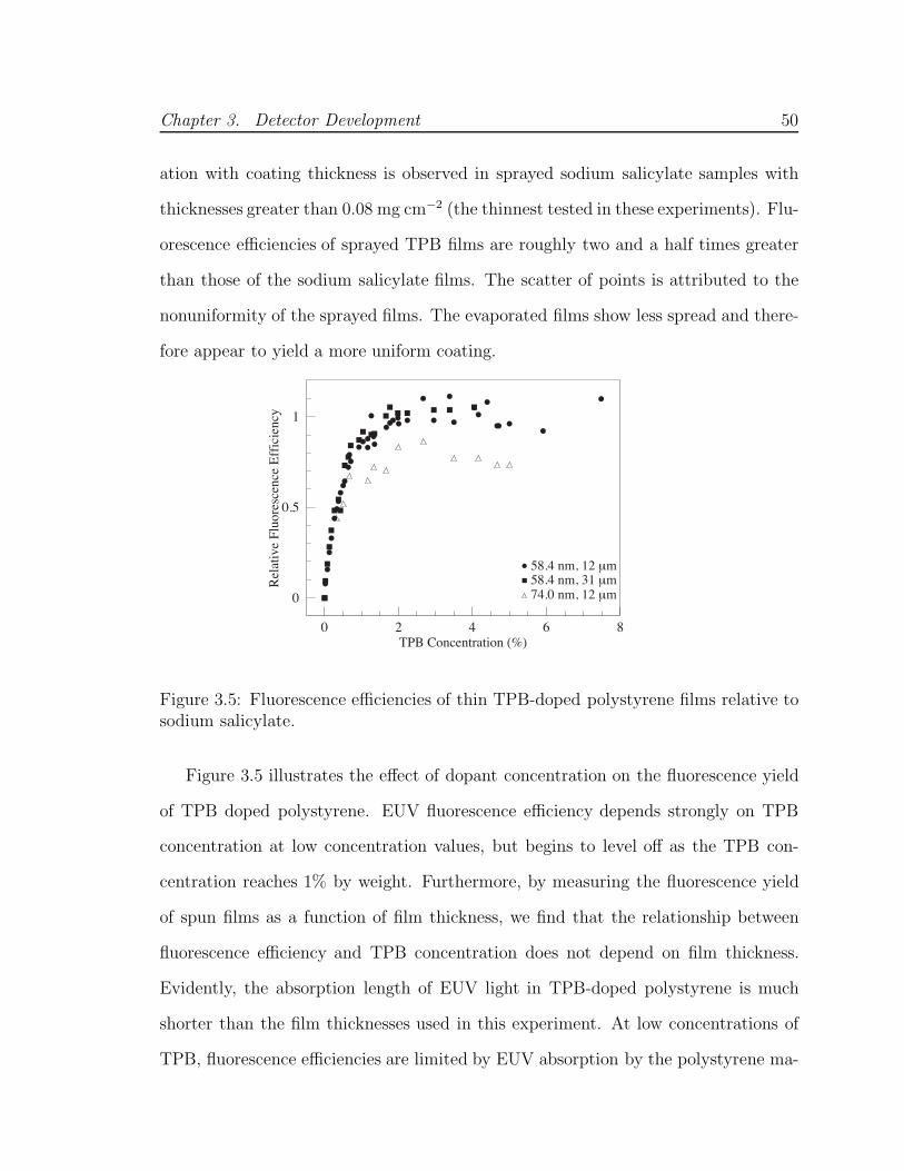
Chapter 3. Detector Development 50
ation with coating thickness is observed in sprayed sodium salicylate samples with
thicknesses greater than 0.08 mg cm−2 (the thinnest tested in these experiments). Flu-
orescence efficiencies of sprayed TPB films are roughly two and a half times greater
than those of the sodium salicylate films. The scatter of points is attributed to the
nonuniformity of the sprayed films. The evaporated films show less spread and there-
fore appear to yield a more uniform coating.
0
0.5
1
0 2 4 6 8TPB Concentration (%)
Rel
ativ
e Fl
uore
scen
ce E
ffic
ienc
y
58.4 nm, 12 µm58.4 nm, 31 µm74.0 nm, 12 µm
Figure 3.5: Fluorescence efficiencies of thin TPB-doped polystyrene films relative tosodium salicylate.
Figure 3.5 illustrates the effect of dopant concentration on the fluorescence yield
of TPB doped polystyrene. EUV fluorescence efficiency depends strongly on TPB
concentration at low concentration values, but begins to level off as the TPB con-
centration reaches 1% by weight. Furthermore, by measuring the fluorescence yield
of spun films as a function of film thickness, we find that the relationship between
fluorescence efficiency and TPB concentration does not depend on film thickness.
Evidently, the absorption length of EUV light in TPB-doped polystyrene is much
shorter than the film thicknesses used in this experiment. At low concentrations of
TPB, fluorescence efficiencies are limited by EUV absorption by the polystyrene ma-

Chapter 3. Detector Development 51
trix, while the maximum fluorescent yield at higher concentrations is limited by a
second process, presumably excitation quenching of the TPB by the plastic matrix.
PMMA and nitrocellulose based plastic films were found to yield lower fluorescence
efficiencies than polystyrene based films.
Polystyrenes of varying molecular weight and chain termination were tested as
matrix materials, showing no noticeable increase in fluorescence efficiency. Matrix
materials similar to polystyrene were also tested, including PVT and PDMS, yielding
similar results. This stands in contrast to the case of electron scintillators, where it
is found that adding methyl groups to polystyrene can increase fluorescence as much
as 59%[66, 67]. We attribute the lower fluorescence efficiencies of these materials
to the difference in excitation mechanisms: electron scintillators are excited largely
by energy transfer from the matrix to the fluor, while EUV light excites the fluors
directly.
P-terphenyl was also tested in a polystyrene matrix. In order to shift all emitted
light to the visible spectrum, a small (1500 ppm) amount of POPOP[68] was added.
The relatively high fluorescent yield of TPH doped polystyrene suggests that widely
used electron scintillators, usually doped with TPH and POPOP, could be used to ef-
ficiently detect EUV radiation. TPB is however the superior fluor for this application
because of its high fluorescence efficiency and because it is less likely to crystallize in
the film than TPH or DPS, allowing greater optical clarity.
In summary, fluorescence efficiencies of evaporated, sprayed, and doped plastic
films at incident wavelengths of 58.4 nm and 74.0 nm were measured. Optimum
coating thicknesses and dopant concentrations have been found for these films. We
have found that the thick evaporated films necessary for efficient soft UV detection can
be replaced by thinner, less opaque films when detecting EUV radiation. Evaporated
Chapter 3. Detector Development 52
films of TPB, PTP, and DPS have been found to yield especially high fluorescence
efficiencies. Doped plastic films are a useful alternative to evaporated films. Although
they have lower fluorescence efficiencies than comparable evaporated films, they can
be index matched to plastic light guides, avoiding the need for a secondary waveshifter
for light guide coupling. In addition, tubes coated with transparent plastic films
show significantly better transmission than tubes coated by evaporation, which can
be an advantage. These clear films could also find use as sensitive coatings for EUV
imaging systems, where low scattering and high transmission of the fluorescent light
are important.
3.2 Fiber Cells
Our first cells built for detecting neutron decays in liquid helium were constructed
using TPB and wavelength-shifting fibers. The idea was that the TPB would convert
the EUV scintillation light from the helium into blue visible light, and then the fibers
would convert the blue light to green light within their cores, trapping the green light
and transporting it out of the cryogenic apparatus. The number of photoelectrons
detected for each beta event can be expressed as
N = Y F (1 − S)Ce−�/�attS
1 − R(1 − S)Q
where Y is the EUV photon yield of the liquid helium, F is the fluorescence efficiency
of the wavelength shifting fluor, S is the fraction of the wall surface covered by the
wavelength shifting fiber, C is the conversion and capture efficiency of the wavelength
shifting fiber, � is the length of the fiber, �att is the attenuation length of the fiber,
R is the reflectivity of the fluor coating, and Q is the quantum efficiency of the light
detector.

Chapter 3. Detector Development 53
TPB on Gore-tex
Wavelength-shifting fibers
Figure 3.6: A fiber cell is built from pair of wavelength shifting fibers and a sheetof Gore-tex with TPB evaporated on its inside surface. The fibers are held in placewith three boron nitride rods (not shown).
In our initial testing, the detection cells were each 15 cm long, and consisted of a
Gore-tex sheet, three boron nitride rods, and two wavelength shifting optical fibers8.
The fibers were bent into a double helix of diameter 32 mm and held in position
using the BN rods. The Gore-tex was coated on one surface with evaporated TPB
and wrapped into a tube9. This tube of Gore-tex, with TPB on its inner surface,
was placed around the wavelength shifting fiber helix and held in place using Mylar
tape. The detection cell assembly was then slid into a G-10 tube of inner diameter
38 mm. The fibers were held in place with three 3 mm x 3 mm x 150 mm rods of
boron nitride, with 24 holes drilled in them (one every 6 mm). Thus each fiber had
80.8 mm diameter double-clad Y11(250) fibers from Kuraray.
9Gore-tex gasketing material purchased from Big River Rubber and Gasket,Owensboro, KY (800) 626-7030 (www.bigriverrubber.com)

Chapter 3. Detector Development 54
Table 3.3: Results for a variety of tests using WLS fiber based cells. Tests using theCs-137 source could not be normalized per unit of energy deposition, as Cs-137 is anintense gamma as well as beta emitter. Here, � stands for the length of each fiber andσ stands for the TPB coverage on the Gore-tex sheet.
Test � σ PMT Source Count rate Counts per Remarks
(m) (µg/cm2) (s−1) 250 keV β
1 0.9 55 8644 Cs-137 17881 -
2 0.9 60 8644 Cs-137 13507 - DPS used
3 0.9 58 8644 Cs-137 16281 -
4 0.9 0 8644 Cs-137 1493 -
5 0.8 95 8644 Cs-137 25158 - d = 12 mm
6 0.9 173 8644 Cs-137 28578 -
7 2.8 143 8644 Cl-36 2976 3.25
8 2.8 240 R943-02 Cl-36 2613 2.83 thru window
9 2.8 231 R943-02 Cl-36 3597 3.89 ball lens
10a 3.9 160 R943-02 Cl-36 2153 2.33 PMT 1
10b R943-02 1796 1.94 PMT 2
10c 457 0.50 Coincidence
12 coils, bent into a diameter of 32 mm. The construction of a fiber cell is shown in
Figure 3.6.
Table 3.3 describes the series of tests on fiber cells that were completed in the
summer of 1997. Tests 1 to 6 were done in a small dewar with a narrow neck, filled
directly with liquid helium from storage dewar. A 137Cs source could be raised and
lowered vertically within the cell, allowing one to compare signals with and without
helium excitation in the detection region. The Cs source emitted betas with an

Chapter 3. Detector Development 55
endpoint energy of 514 keV, and its activity was measured to be 2830 betas per second
using a pancake counter10. Tests using the Cs-137 source could not be normalized
per unit of energy deposition, as Cs-137 is an intense gamma as well as beta emitter.
One end of each fiber exited the dewar and pushed up against the front window of a
single 19 mm diameter PMT11 with heightened long wavelength response (quantum
efficiency of about 12% at 500 nm). The cell tube was open at the bottom to allow
liquid helium to enter the detection region. It was shown that TPB worked better
than DPS (diphenyl stilbene, another fluor used for wavelength shifting EUV light),
and that a 6 mm coil spacing worked better than a 12 mm coil spacing. By doing one
run without any TPB on the Gore-tex, It was observed that the liquid helium from
the storage Dewar fluoresced somewhat in the visible; this can be explained by frozen
air impurities in the helium. Fluorescence from impurities in liquid helium has been
observed in previous work[33].
Tests 7 to 9 were done in a tall 12.7 cm dewar. In this apparatus (see Figure 3.7),
the G-10 tube was closed at the bottom with a copper flange. The fibers traveled up
through the tube to Swagelok feedthroughs and exited the cryogenic apparatus. The
G-10 tube could be filled with helium separately from the surrounding helium bath,
and this allowed us to test cells using highly purified helium from a gas bottle. After
filling the region outside the G-10 tube with liquid helium from a storage Dewar, the
outer region could be pumped to lower temperatures, allowing the pure helium to
be condensed within the cell. By varying the rate of pumping, the temperature of
the cell could be lowered to 1.8 K. A superconducting wire level gauge allowed us to
measure the level of helium within the G-10 tube.
10calibrated to within 10%
11Burle 8644

Chapter 3. Detector Development 56
36
Cryogenic helium
G-10 tube
Gore-tex tube
20 cm
Cl betasource
Copperendcap
Sample helium
Copper cup
Evaporated TPB film
Wavelengthshifting fiber
Figure 3.7: Diagram of the cryogenic apparatus used to test fiber-based detectioncells.
Tests 7 to 9 were done using a 36Cl source, whose beta decay spectrum (average
energy 252 keV, maximum energy 710 keV) mimicked closely that of the neutron.
This source had an intensity of 920 betas per second (measured using a pancake
counter), and could be lowered or raised witin the cell using a motion feedthrough
at room temperature at the top of the apparatus. By alternately lowering the source
into a copper cup at the bottom of the tube and raising it into the center of the
detector, a measurement of the helium scintillations could be performed. After doing
a first test using the 19 mm photomultiplier, we switched to a photomultiplier with
better response in the green12. This photomultiplier had to be cooled to achieve low
dark counts13, and had a recessed GaAs photocathode, making it more difficult to
couple it to the fiber effectively. At first we simply sent the fiber light through an
12Hamamatsu R943-02, with a quantum efficiency of 19% at 500 nm.
13Peltier cooler purchased from Products For Research.

Chapter 3. Detector Development 57
acrylic window, but later we found that a 10 mm ball lens could be used to focus
the light from the fiber into the photocathode. With a TPB concentration of about
0.2 mg cm−2 we found that we could detect about 3.9 counts per β particle. This is
comparable to the count rate predicted with the following assumptions:
Y = 11,000 ± 1,000 EUV photons for a 250 keV beta.
F = 1.6 ± 0.1 for TPB.
S = 0.12 ± 0.01 for a fiber coil every 6 mm.
C = 0.025 ± 0.002 for the conversion and capture efficiency of the Y11 fiber (one
end).
� = 2.8 ± 0.2 m (the total fiber length from the center of the detector).
�att = 2.9 ± 0.2 m (the attenuation length of the wavelength shifting fiber).
R = 0.75 ± 0.10 (estimated reflectivity of TPB)
Q = 0.13 ± 0.02 (quantum efficiency of the R943-02 multiplied by optics efficiency)
These assumptions predict a total collection of 6.7 +2.7−2.0 photoelectrons per 250 keV
beta. This is somewhat greater than the observed 3.9 counts per beta. Obviously the
large number of assumptions that go into this calculation make it rather uncertain.
The error is dominated by the uncertainty in the reflectivity of TPB-coated Gore-tex.
We have not yet measured this quantity; plain Gore-tex is known to have a reflectivity
of 90%; the evaporation of TPB makes it visibly less white.
The cell used for the first attempt to detect trapped neutrons was 30 cm long
(twice as long as the cells initially tested), with two fibers wrapped in helixes of
opposite sense. Two sets of 15 cm long BN rods (6 rods total) and two Gore-tex
sheets were used. Each boron nitride rod had 24 holes drilled through it, and each
fiber was wound through two sets of boron nitride rods, so each fiber had a total
Chapter 3. Detector Development 58
of 24 coils. All four fiber ends were taken out of the cryogenic apparatus. At first,
all four fibers were fed into a single Hamamatsu R943-02 photomultiplier. However,
we soon found that the neutron trapping apparatus suffered from a large quantity of
neutron-induced luminescence, and we began running in coincidence, with the two
ends of each fiber fed into its own PMT.
After approximately one month of beam time and failing to observe trapped neu-
trons because of the high levels of luminescence, we tested the efficiency of the larger
cell. This test (number 10 in the table above) revealed that the light yield in each
PMT was decreased significantly by the increased fiber length. The decrease in light
yield is consistent with the 2.9 m light attenuation length in the wavelength shifting
fibers. We found that only about half of the decay events were detectable in coin-
cidence. Altogether, the fiber-based cells of the type used in the attempt to detect
trapped neutrons yielded 4.27 photoelectrons per 36Cl decay (summing the yield in
the two photomultipliers). Since a large fraction (33 ± 10 %) of the photoelectrons
came from triplet He∗2(a
3Σ+u) decay, this photoelectron yield must be multiplied by
66% ± 10 % to find the total number of photoelectrons in the prompt pulse. This
fraction is estimated from the intensity of triplet molecule decay (see Chapter 4). As-
suming a PMT quantum efficiency of 19 ± 1% and a light collection efficiency of 40 ±
10% for transport of the light from the fiber coils, through the 1.5 m of fiber between
the coils and the photomultiplier, into the ball lens, and onto the PMT photocathode,
one finds that the fiber cells yielded 224 ± 60 photons/MeV.
While the fiber-based cells never were demonstrated to have high light collection
efficiencies, this sort of design may be useful in the future. Because the fiber has
a small cross-section area, it can be snaked out of an apparatus without taking up

Chapter 3. Detector Development 59
much room14. The fiber design was used initially in the neutron trapping experiment
because it was felt that the neutron beam should not be stopped within the apparatus
because of neutron activation and heat load issues. With this contraint removed, we
turned to a second detector design, developed largely at HMI, Berlin by Klaus Habicht
and Bob Golub[69].
3.3 Tube Cells
The second sort of detector insert used in the neutron trapping experiment was based
on acrylic tubes whose inside surfaces were coated with TPB-doped polystyrene. This
mixture was tested using the fluorescence efficiency rig (see Section 3.1) and found
to have good EUV-to-visible conversion properties (F of 40%). Polystyrene doped
with TPB is transparent and can be index matched to light guides, allowing efficient
transportation of visible light out of the detection region. Based on this discovery,
our collaborators at HMI began using TPB-doped polystyrene coated on the inside
surface of acrylic tubes as a basis for helium scintillation detection [69].
TPB DopedPolystyrene
250 mK4 K
77-300 KBN
NeutronCollimator Beam Dump
5 cm
40 cm60 cm
PMTs
liquid helium bath2He *
e–�
γ – 80nm
γ – 430nm
Acrylic Tube
Figure 3.8: A sketch of the detector insert used in the 1999 neutron trapping run.
14The neutron EDM experiment may use fiber-based detection because the detec-tion cell must be surrounded by magnetic shielding, whose effectiveness would becompromised by any large holes.
Chapter 3. Detector Development 60
After we discovered large amounts of neutron-induced luminescence in our cell, we
concluded that a more efficient detector insert was needed to boost the signal out of
the single photoelectron noise. We abandoned the requirement that the neutron beam
be able to pass through the apparatus, abandoned the wavelength shifting fiber-based
cells, and instead investigated the possibility of using an acrylic tube-based design.
In this approach (see Figure 3.8), the TPB-polystyrene coating converts the EUV
scintillation light to blue light. About half of the blue light is then trapped in the
tube walls, and a fraction of this light makes it to the end of the tube. This light
then passes into an acrylic light guide, passing around a black boron carbide disc (the
neutron beam dump). The light signal continues through two windows (at 200 mK
and 4 K) and a light guide at 77-300 K, and then is detected using photomultiplier
at room temperature.
The photomultiplier we used for these measurements was the Burle 8850. This
5 cm diameter tube has a bialkali photocathode and is maximally sensitive at 400
nm, well matched to the emission of TPB. But its most interesting property is its low
gain dispersion. The term “gain dispersion” refers to the uncertainty in the size of
the electronic pulse made by the photomultiplier, given a number of photoelectrons
emitted by the photocathode. Because the gain dispersion of the Burle 8850 is so
low, it is possible to distinguish one photoelectron events from larger events, based
on the size of the signal from the anode of the PMT. This property of the Burle
8850 is illustrated in Figure 3.9. By requiring that events register more than one
photoelectron, a cut on neutron-induced luminescence was possible. Of course, it was
then necessary to ensure that actual neutron decays produced well more than a one
photoelectron signal.
To optimize the design of the tube-based detector inserts, an apparatus was built
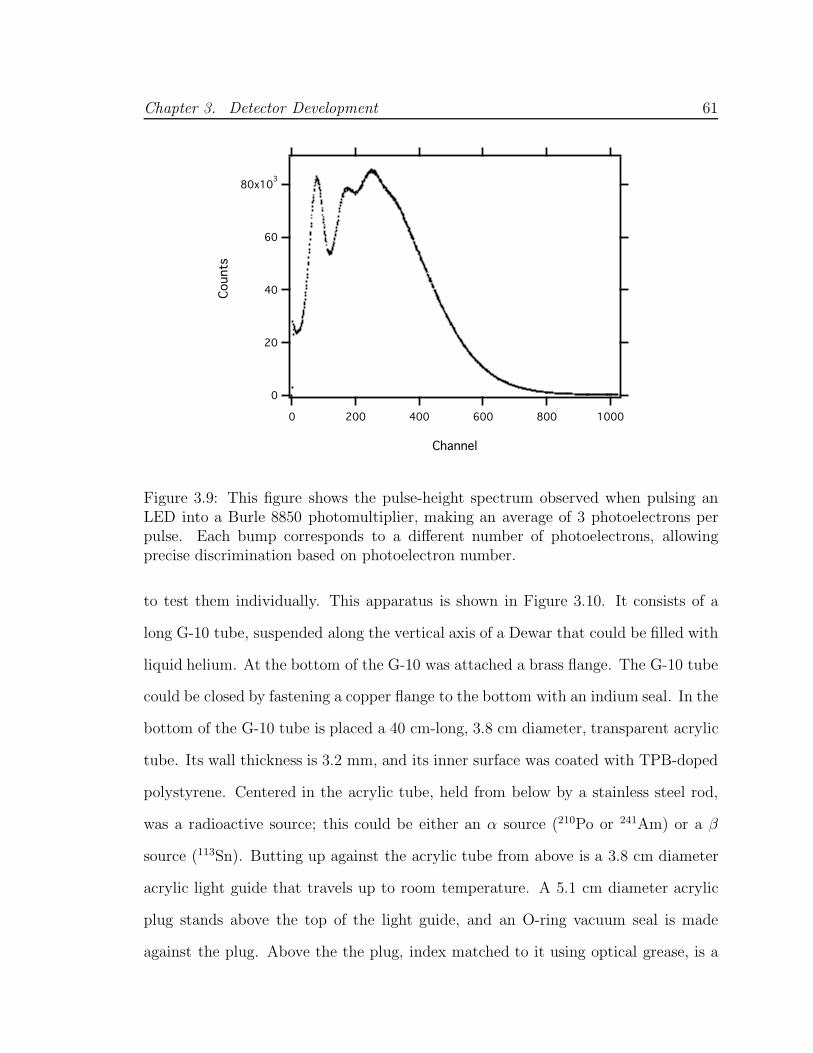
Chapter 3. Detector Development 61
80x103
60
40
20
0
Coun
ts
10008006004002000
Channel
Figure 3.9: This figure shows the pulse-height spectrum observed when pulsing anLED into a Burle 8850 photomultiplier, making an average of 3 photoelectrons perpulse. Each bump corresponds to a different number of photoelectrons, allowingprecise discrimination based on photoelectron number.
to test them individually. This apparatus is shown in Figure 3.10. It consists of a
long G-10 tube, suspended along the vertical axis of a Dewar that could be filled with
liquid helium. At the bottom of the G-10 was attached a brass flange. The G-10 tube
could be closed by fastening a copper flange to the bottom with an indium seal. In the
bottom of the G-10 tube is placed a 40 cm-long, 3.8 cm diameter, transparent acrylic
tube. Its wall thickness is 3.2 mm, and its inner surface was coated with TPB-doped
polystyrene. Centered in the acrylic tube, held from below by a stainless steel rod,
was a radioactive source; this could be either an α source (210Po or 241Am) or a β
source (113Sn). Butting up against the acrylic tube from above is a 3.8 cm diameter
acrylic light guide that travels up to room temperature. A 5.1 cm diameter acrylic
plug stands above the top of the light guide, and an O-ring vacuum seal is made
against the plug. Above the the plug, index matched to it using optical grease, is a
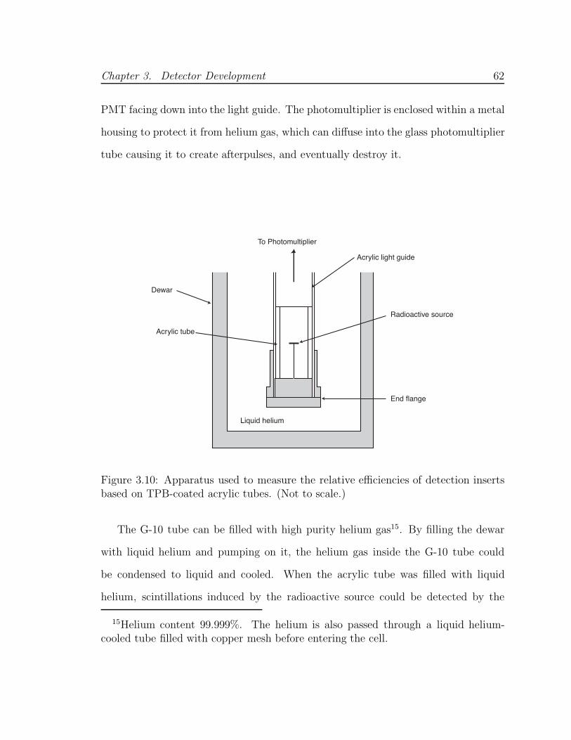
Chapter 3. Detector Development 62
PMT facing down into the light guide. The photomultiplier is enclosed within a metal
housing to protect it from helium gas, which can diffuse into the glass photomultiplier
tube causing it to create afterpulses, and eventually destroy it.
Dewar
To Photomultiplier
Acrylic light guide
Acrylic tube
Radioactive source
Liquid helium
End flange
Figure 3.10: Apparatus used to measure the relative efficiencies of detection insertsbased on TPB-coated acrylic tubes. (Not to scale.)
The G-10 tube can be filled with high purity helium gas15. By filling the dewar
with liquid helium and pumping on it, the helium gas inside the G-10 tube could
be condensed to liquid and cooled. When the acrylic tube was filled with liquid
helium, scintillations induced by the radioactive source could be detected by the
15Helium content 99.999%. The helium is also passed through a liquid helium-cooled tube filled with copper mesh before entering the cell.

Chapter 3. Detector Development 63
photomultiplier at room temperature. The PMT signal was fed to a charge preamp16
and thence to a scintillation amplifier17 and multichannel analyzer. Pulse-height
analysis was performed on the resulting distribution of signal sizes. By comparing
the scintillation peak position with the position of the one photoelectron peak, the
average number of photoelectrons made by a scintillation events could be determined.
The construction of the acrylic tube could then be varied in attempts to optimize the
design of the detector insert.
The acrylic tubes were coated with TPB-doped acrylic through a careful proce-
dure. First, the acrylic tube was cut to length (40 cm) and its ends polished. Only
ultraviolet transmitting grade (UVT) acrylic was used to maximize blue light trans-
mission. Then a mixture of research grade toluene, crystalline TPB, and polystyrene
pellets was stirred and heated within a beaker. When the mixture was dissolved and
warm, the acrylic tube was lowered about 1 cm into the liquid. The top of the tube
was covered with a rubber plug with a hole in the center. Leading from the hole
was a rubber hose with a valve midway thru its length, and the far end of the hose
terminated at a pump. By carefully throttling the valve, the liquid could be sucked
up into the acrylic tube. After a few seconds, the pump was shut off and the liquid
level allowed to slowly drop (over a 20 second period). The tube was then set aside
to dry. When dry, the tube was wrapped with Tyvek paper18 to protect the tube.
A variety of tests were performed on the acrylic tube-based detector inserts. These
tests are summarized in Table 3.4. Most of the early tests were done using a high
energy alpha source, so as to have lots of scintillation signal. It was found that a
16Canberra 2005
17Shaping width 1 µs
18DuPont Chemical Corporation.

Chapter 3. Detector Development 64
Table 3.4: Results for a variety of tests using acrylic tube-based cells
Test Date Source Excitation PMT Peak signal Remarks
(p.e.)
1 6/20/98 Po-210 5.3 MeV α 8850 177 HMI cell, 40 % TPB
2 6/22/98 Po-210 5.3 MeV α 8850 73 40% TPB, center blocked
3 6/24/98 Po-210 5.3 MeV α 8850 112 4% TPB
4 6/26/98 Po-210 5.3 MeV α 8850 146 TPB on Gore-tex
5 9/20/98 Am-241 5.5 MeV α 8850 147 12% TPB
6 9/20/98 Am-241 5.5 MeV α 8850 112 4% TPB
7 2/5/99 Am-241 5.5 MeV α 8850 145 8% TPB
8 2/5/99 Am-241 5.5 MeV α 8850 144 8% TPB, dewar helium
9 2/11/99 Am-241 5.5 MeV α 8850 40 2% TPB, center blocked
10 2/13/99 Am-241 5.5 MeV α 8850 72 30% TPB, center blocked
11 2/23/99 Sn-113 364 keV β 8850 18.5 40% TPB
12 2/24/99 Sn-113 364 keV β 8850 5.5 neutron cell; 40% TPB
13 2/28/99 Am-241 5.3 MeV α 8850 62 40% TPB, center blocked
14 3/6/99 Sn-113 364 keV β 8850 8.5 40% TPB, center blocked
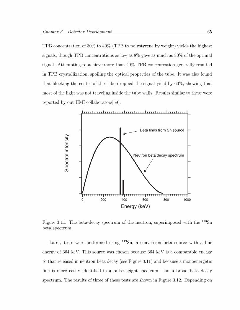
Chapter 3. Detector Development 65
TPB concentration of 30% to 40% (TPB to polystyrene by weight) yields the highest
signals, though TPB concentrations as low as 8% gave as much as 80% of the optimal
signal. Attempting to achieve more than 40% TPB concentration generally resulted
in TPB crystallization, spoiling the optical properties of the tube. It was also found
that blocking the center of the tube dropped the signal yield by 60%, showing that
most of the light was not traveling inside the tube walls. Results similar to these were
reported by out HMI collaborators[69].
Spe
ctra
l int
ensi
ty
10008006004002000
Energy (keV)
Beta lines from Sn source
Neutron beta decay spectrum
Figure 3.11: The beta-decay spectrum of the neutron, superimposed with the 113Snbeta spectrum.
Later, tests were performed using 113Sn, a conversion beta source with a line
energy of 364 keV. This source was chosen because 364 keV is a comparable energy
to that released in neutron beta decay (see Figure 3.11) and because a monoenergetic
line is more easily identified in a pulse-height spectrum than a broad beta decay
spectrum. The results of three of these tests are shown in Figure 3.12. Depending on

Chapter 3. Detector Development 66
whether the center of the cell was blocked with a black neutron beam dump, either
8.5 or 18.5 photoelectrons could be detected per 113Sn decay. When one of these cells
was placed within the neutron trapping experiment along with the 113Sn source, an
average of 5.5 photoelectrons was detected. The decrease in average pulse size was
due to a more complicated, less efficient, set of optics for transporting the light to
room temperature.
Cou
nts
(nor
mal
ized
)
2520151050Photoelectrons
2
1
3
Figure 3.12: Three calibration runs of acrylic tube-based scintillation detectors. A113Sn source, emitting β particles at 364 keV, is used to create pulses of EUV lightin the liquid helium. Curve 1 shows the response of a cell used to detect trappedneutrons in April-May 1999. Curve 2 shows the response of a similar cell tested ina cell testing rig. Only light passing through the acrylic wall is allowed to pass; therest is clocked by a black neutron beam stop. Curve 3 shows the response of a cellwithout the center blocked.
The intensity of the scintillation signal was also measured as a function of source
position. By attaching an alpha source to a string and installing an arrangement

Chapter 3. Detector Development 67
of hooks within the cell over which the string traveled, the vertical position of the
alpha source could be varied along the length of the acrylic tube. This roughly linear
variation in signal is shown in Figure 3.13.
100
80
60
40
20
0
photo
ele
ctro
ns
403020100
position (cm)
Figure 3.13: Position dependence of the scintillation signal for the tube-based detec-tor.
The efficiency of the light guide in the tube cell testing rig was measured by
attaching a piece of organic scintillator with a beta line source attached, alternately
to the end of the light guide (so that the light from the scintillator traveled up the
light guide and into the PMT) and directly to PMT itself. It was found that the light

Chapter 3. Detector Development 68
guide is 31% efficient. Given that the Burle 8850 has approximately a 20% quantum
efficiency for detecting blue light, it follows that about 140 photons per 113Sn beta
event are released from the end of the acrylic tube if its center is blocked, and about
300 photons if it is not. Given the high EUV yield of liquid helium (22,000 photons
per MeV for β particles) it follows that only 3.8% of the EUV photons released in
the liquid helium result in a blue photon exiting upward into the light guide, and
this number drops to 1.8% if the center is blocked. This low yield of blue photons
is a combination of the fluorescence yield of TPB doped polystyrene (approximately
25%) and the transmission of the acrylic tube (6.9% in the tube wall, 8.3% down the
center). Of course these numbers would be different for a different acrylic tube; a
larger wall thickness or shorter tube would increase these numbers significantly.
3.4 Gore-tex Cells
One of the results (number 4) shown in Table 3.4 revealed that a cell built using a
sheet of Gore-tex rolled into a tube, with TPB evaporated on its inside surface, could
also perform well as a detector. However, since there is no tube wall to propagate light
around the beam dump, all the light extracted from a Gore-tex cell must come down
the center. Therefore, a black beam dump makes the use of a Gore-tex cell impossible.
However, after 1999 we put significant effort into developing a transparent beam
dump, one that could both absorb the neutron beam and pass scintillation light.
Eventually we chose to use a cylinder of high purity boron oxide B2O3 as a beam
dump. The program of transparent beam dump development is described in Chapter
5.
Because our new magnetic trap has a larger bore diameter (105 mm) than the
previous one (51 mm), the light emitted from a Gore-tex cell is now more easily

Chapter 3. Detector Development 69
collected. In addition, evaporated TPB has a higher fluorescence efficiency than
TPB-doped polystyrene. For larger bore detectors, with easier optical access to the
trapping region, the Gore-tex cell proved superior. The number of photoelectrons
collected using this detector insert is higher than in previous cell designs. In March,
2001, a calibration run was performed in the neutron trapping apparatus which was
equipped at the time with this type of detector. Using a Burle 8854 photomultiplier
(quantum efficiency 17%) a prompt peak of 35 photoelectrons was seen. The optics
transmission efficiency at the time is estimated to be 49% (this was before the optics
were modified to reduce infrared heating, see Chapter 5); thus about 1150 photons
leave the Gore-tex tube per MeV of beta energy deposition. This type of detector
was used to detect trapped neutrons in August, 2001, and will be discussed in more
detail in Chapter 5.
Table 3.5 summarizes the results of this chapter. It shows the efficiencies of the
various detector technologies for turning helium scintillation events into detector pho-
toelectrons. The “Photons/MeV” column specifies the estimated number of photons
that escape the trapping region. The “Optics” column specifies the estimated chance
that a photon passes from cryogenic temperatures to a detector at room tempera-
ture. The “QE” column specifies the quantum efficiency for the photomultiplier used
in that measurement. The “P.E./MeV” column specifies the estimated efficiency for
turning a single beta excitation in the liquid helium into prompt photoelectrons in
the detector.

Chapter 3. Detector Development 70
Table 3.5: Summary of detector efficiencies
Detector type Photons/MeV Optics QE P.E./MeV
Wavelength shifting fibers 224 ± 60 40 ± 10% 19 ± 1% 17 ± 2.6
Acrylic tube (center blocked) 377 ± 57 31 ± 3% 20 ± 2% 23.4 ± 1.4
Acrylic tube (center open) 819 ± 116 31 ± 3% 20 ± 2% 50.8 ± 1.4
TPB evaporated on Gore-tex 1150 ± 203 49 ± 5% 17 ± 2% 96 ± 8.0

Chapter 4
The Physics of Liquid Helium
Scintillations
This chapter describes several experiments designed to investigate the time depen-
dence of EUV fluorescence following ionizing radiation events. It is found that both
alpha and beta particles create an afterpulsing tail that decays exponentially with
a 1.7 µs time constant. It is speculated that this exponential tail results from the
reaction of He(21S) atoms with the liquid helium. Another discovery is that alpha
particles create an additional fluorescence tail whose intensity varies as 1/time, that
the intensity of this tail depends on the temperature of the superfluid helium, and
that this long-lived scintillation tail is not created by beta particles to any substantial
degree. It is also found that liquid helium phosphoresces on the time scale of many
seconds; this remarkable property is a result of the radiative de-excitation of triplet
helium excimers and exhibits an exponential time constant of 13 ± 2 s.
71

Chapter 4. The Physics of Liquid Helium Scintillations 72
4.1 Prompt Scintillation
After an ionizing particle passes through liquid helium, a large number of excited
atoms, free electrons, and ions are created. The energy deposition per unit length
depends strongly on the charge and mass of the exciting particle. This variation
in dE/dx has a big effect on the dynamics of the particles created by the track.
For example, because a high energy electron deposits on average 50 eV/µm and the
average energy to produce an ion-electron pair is is 42.3 eV, it follows that ionization
events are on average 850 nm away from each other. With an average separation of
10 nm between the ion and its lost electron, it is clear that ion-electron pairs are well
separated under beta excitation[70]. But under alpha excitation, this is not the case.
If the excitation is an alpha source, the deposition is 2.5 × 10⁴ eV/µm, and therefore
the average spacing between events is only 2 nm.
In any case, the excited atoms, electrons, and ions quickly thermalize with the
liquid helium. The electron, once thermalized, forms a bubble in the liquid, pushing
away surrounding helium atoms. Experiments on electron bubbles show that the
bubble formation happens within 4 ps[71]. The bubble displaces a large number of
helium atoms; therefore the electron has a large effective mass (m ∼ 240 helium
atoms), and moves slowly throught the liquid.
The He+ ion reacts within 100 - 500 ps with the surrounding helium to form He+2 .
It forms in a high vibrational state[72, 73], but soon drops to a lower vibrational state
through inelastic collisions with surrounding helium atoms. Then the He+2 ion can
react again to form a triatomic ion:
He+2 + He → He+
3 .
This ion is thought to then form the core of a helium “snowball”, which forms within
5 ps[74]. In a snowball, surrounding helium atoms are attracted to the He+3 ion. The
Chapter 4. The Physics of Liquid Helium Scintillations 73
snowball has an effective mass of 40 helium atoms and thus has a large effective mass
(though not as large as the electron bubble).
As mentioned earlier, the average distance between the electron bubble and its
parent ion is 10 nm. Based on this initial separation and the effective snowball mass,
the average recombination time is 0.3 ns for electron excitation. The ion production
and recombination process has been studied carefully by Benderskii et al. [75]. A
helium snowball will react with a free electron as follows:
(He+3 )snowball + (e−)bubble → He2 + He.
This reaction is the source of large numbers of He2 molecules, produced in both
triplet and singlet states. While the ratio of singlet and triplet formation rates found
in in low-density gases normally approaches a 1:3 statistical weight, it is found that
molecular formation in liquid helium exhibited relatively more singlet formation if
the helium is excited by a high energy electron. This is attributed to the fact that
most electrons do not escape from their parent helium atom following ionization of
singlet ground state helium atoms. This makes it overwhelmingly likely that a given
liberated electron will recombine with its parent if the excitation is produced by a
high energy electron. However, if the excitation is created by an alpha particle, then
the ions are created much closer together, Then it is much more likely that a given
electron will not recombine with its parent, and the triplet/singlet ratio will approach
3:1.
The claim that ionic recombination is the chief source of He2 molecules is but-
tressed by the measurements done by Roberts et al.; in these experiments an electric
field applied to the helium strongly attenuates the scintillation pulse (as much as
60%).
Even if there is a high electric field, significant scintillation is produced by helium

Chapter 4. The Physics of Liquid Helium Scintillations 74
atoms. Excited atoms are also produced, 0.45 per ion[76]. Again, because the initial
helium atom is a singlet state, the excited atom is also likely to be in a singlet state.
Of these, 83% are in the singlet state, and 17% are in the triplet state, when excited by
electrons. It is well known that triplet atoms willl react with the surrounding helium
to form triplet He2 molecules. There is however a 60 meV activation energy for
this reaction to occur[43]. It is believed that the high liquid density makes molecule
formation more likely, as the He∗(23S) - He(11S) potential can be affected by the
presence of a third atom. It has been found that He∗(23S) atoms react to form
He∗2(a
3Σ+u ) in 15 µs, but the time required to form He2(A
1Σ+u ) molecules from He(21S)
atoms has not yet been measured[40, 41].
In our case (with no electric field present), the prompt pulse of EUV light created
immediately after an ionizing radiation event is due mainly to the radiative decay
of He2(A1Σ+
u ) molecules, which have been formed largely through electron recombi-
nation. The shape of the initial scintillation pulse was studied carefully by Klaus
Habicht, and a more detailed discussion can be found in his thesis[69]. The pulse
shape that we observe has a fast rise time (about 5 ns), and a 1/e decay time of 10
ns. This 10 ns decay time represents an upper limit on the lifetime of the He2(A1Σ+
u )
molecule molecule, but certainly includes other effects such as the emission lifetime
of the TPB and the response time of the photomultiplier.
4.2 Afterpulsing
After the prompt pulse eliminates the He2(A1Σ+
u ) molecules, other electronic excita-
tions remaining are singlet atoms, triplet atoms, and triplet molecules. The interac-
tions between these species within the ionizing track can result in more scintillation
light following the prompt component. Because the excitation density depends on

Chapter 4. The Physics of Liquid Helium Scintillations 75
the kind of ionizing radiation, different ionizing particles can exhibit different pulse
shapes. As the excitation track spreads in size and excitations are removed, the rate
of reactions decreases. The pulse shape and intensity can therefore depend on the
mobility and density of these excitations.
We observe a strong exponential tail following the prompt pulse, with a 1.7 µs
lifetime. This tail is created from both alpha and beta excitation. An experimental
trace illustrating this decay is shown in Figure 4.1. This trace was taken by triggering
a multichannel scalar (MCS) 1 on the prompt pulses from a 113Sn source in a Gore-tex-
based detector (see Chapter 3) and counting single photon afterpulses. The average
number of photoelectrons in the main pulse was 12. The cell used in this test is the
same cell used to detect magnetically trapped neutrons in August, 2001, and was made
of a Gore-tex tube coated with an evaporated layer of TPB. The cell was viewed by a
photomultiplier with high gain and good single photoelectron resolution2. It should
be noted that this 1.7 µs lifetime is demonstrably not a result of a slow component
in the TPB fluorescence decay; this can be seen from the results of Klaus Habicht
[69], where it is shown that the scintillation curve in cold gaseous helium exhibits
a considerably different time dependence on µs time scales. One would not expect
the TPB lifetime to depend on whether the cell contains liquid or gaseous helium;
therefore the 1.7 µs lifetime seen here is evidence of a reaction in the helium.
As can be seen from the above fit, the afterpulsing from beta particles fits well
to a single exponential, with a 1.7 µs decay lifetime and total intensity Aτ of 3.3
photoelectrons. This scintillation tail probably derives from a metastable entity re-
acting with the background helium. A plausible candidate is the metastable atom
1SRS model SR430, Stanford Research Systems, Sunnyvale, CA
2Burle 8854 photomultiplier, Burle Industries, Lancaster, PA

Chapter 4. The Physics of Liquid Helium Scintillations 76
2.0
1.5
1.0
0.5
0.0
Cou
nt r
ate
(µs-1
)
20151050Time after main pulse (µs)
Figure 4.1: Afterpulse intensity from a beta source, as a function of time, plus a fitto the function Ae−kt + B, where t is measured in µs. The background B is 0.6005± 0.0004 µs−1, the amplitude A fits to 2.07 ± 0.02 µs−1, and k fits to 0.633 ± 0.005µs−1. This data was taken at a temperature of 250 mK using a Gore-tex cell. There isan average of 12 photoelectrons in the main pulse (first 1.0 µs), and the total intensityof this exponential tail is 3.3 photoelectrons.
He(21S), which has a vacuum lifetime of about 1 second. There is evidence from
spectroscopic measurements of electron-beam excited liquid helium that this partic-
ular atom species reacts with the surrounding helium atoms to form the He2(A1Σ+
u )
molecule, which then can radiatively decay immediately[44]. Though the timescale
of this process has never been measured, a similar reaction with He(23S) atoms has
been shown to occur with a 15 µs characteristic lifetime[41].
This exponential lifetime is also found in alpha-induced scintillations[69]. But
in addition it is found that a second component is present, decaying with a 1/time
dependence. This decay can be seen in Figure 4.2, which shows the decay curve of
afterpulsing in an acrylic tube-based cell. The source of this component is uncertain,
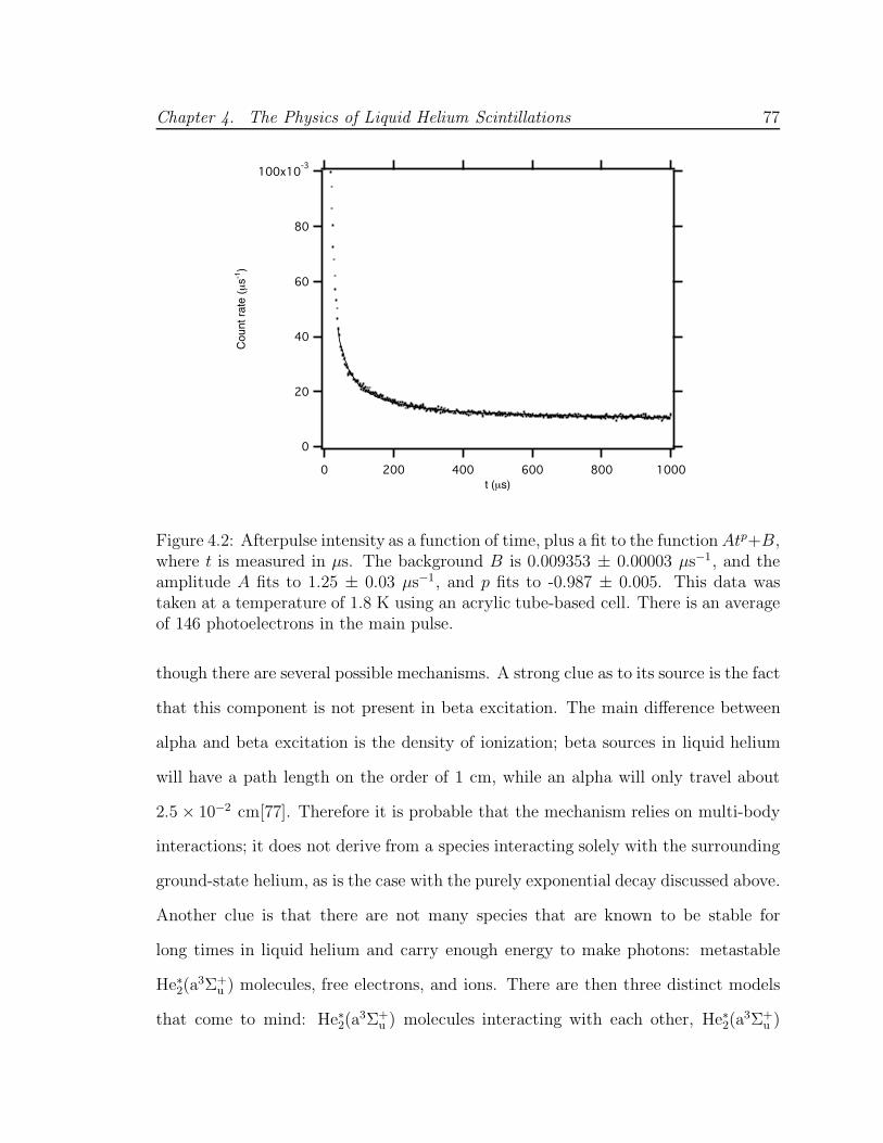
Chapter 4. The Physics of Liquid Helium Scintillations 77
100x10-3
80
60
40
20
0
Cou
nt r
ate
(µs-1
)
10008006004002000t (µs)
Figure 4.2: Afterpulse intensity as a function of time, plus a fit to the function Atp+B,where t is measured in µs. The background B is 0.009353 ± 0.00003 µs−1, and theamplitude A fits to 1.25 ± 0.03 µs−1, and p fits to -0.987 ± 0.005. This data wastaken at a temperature of 1.8 K using an acrylic tube-based cell. There is an averageof 146 photoelectrons in the main pulse.
though there are several possible mechanisms. A strong clue as to its source is the fact
that this component is not present in beta excitation. The main difference between
alpha and beta excitation is the density of ionization; beta sources in liquid helium
will have a path length on the order of 1 cm, while an alpha will only travel about
2.5 × 10⁻² cm[77]. Therefore it is probable that the mechanism relies on multi-body
interactions; it does not derive from a species interacting solely with the surrounding
ground-state helium, as is the case with the purely exponential decay discussed above.
Another clue is that there are not many species that are known to be stable for
long times in liquid helium and carry enough energy to make photons: metastable
He∗2(a
3Σ+u ) molecules, free electrons, and ions. There are then three distinct models
that come to mind: He∗2(a
3Σ+u ) molecules interacting with each other, He∗
2(a3Σ+
u )

Chapter 4. The Physics of Liquid Helium Scintillations 78
molecules interacting with ions or electrons, or from ions and electrons recombining.
Let us examine each of these models in turn:
Metastable-metastable interactions
Metastable-metastable interaction is a well known phenomenon in organic scintilla-
tors. In these materials, as in liquid helium, both singlet and triplet states are excited.
And as in liquid helium, the singlet states decay rapidly, leaving triplet states still car-
rying chemical energy from the original ionizing event. Following King and Voltz[78],
the concentration of triplet states cT then evolves as
∂cT (r, t)
∂t= DT ∇2
rcT (r, t) − χttc2T (r, t) − 1
τT
cT (r, t),
where DT is the triplet diffusion coefficient, χtt is the triplet destruction coefficient,
and τT is the triplet lifetime. In this model, triplet destruction can feed singlet
creation. If triplet destruction can create singlets with rate ktt, then light will be
produced at a rate proportional to χttktt. Thus triplet-triplet interactions can feed
a short-lived scintillation component. In liquid helium, an appropriate mechanism
for triplet-triplet annihilation is Penning ionization, for which the reaction rates have
been measured previously[40]. The alpha track in liquid helium is approximately
60 nm in diameter and 2.5 × 10⁻² cm long[70].
The above equation is non-linear, and must be solved using approximation meth-
ods. The triplet decay term 1τT
cT (r, t) can be ignored, as the triplet lifetime is very
long compared to the time scale of the track dynamics. It can also be seen that, in
the pure diffusion equation without triplet annihilation, that the triplet density at
the center of the track decreases with a time constant td = r20/4DT , where r0 is the
initial width of the track, assumed here to be cylindrically symmetric and Gaussian,
Chapter 4. The Physics of Liquid Helium Scintillations 79
i.e.
cT (r, 0) = cT (0)e−(r/r0)2
.
On the other hand, if there were no diffusion, then the density of triplets would
decrease entirely through triplet-triplet destruction with a characteristic lifetime ttt =
1/(χttcT (0)). Depending on whether td or ttt is smaller, either diffusion or annihilation
controls the process.
Under the approximation that the track continues to be Gaussian as the track
expands, the rate of singlet radiation from triplet annihilation I ′(t) can be shown to
be[78]
I ′(t) =kfkttτs
2χttttt
NT (0)[1 + td
2tttln(1 + t
td)]2
(1 + ttd
).
For the case of alpha particles in liquid helium, this expression can be simplified.
After the alpha particle excites the helium, the temperature within the alpha track
rises considerably. If the alpha particle deposits 5.3 MeV in a volume of 8×10⁻¹³cm3
(for a track of radius 30 nm and length .025 cm), then the temperature should rise
to about 2 K. At this temperature, DT should be about 4 × 10⁻⁴cm2s−1[79]. Then
td = r20/4DT = 25 ns. The annihilation time ttt = 1/(χttcT (0)) will be much longer,
about 125 ns, as χtt is 2 × 10⁻¹⁰cm3s−1 at a temperature of 2.0 K (as measured in
electron-bombarded superfluid helium[40]), and the concentration cT should be about
4 × 10¹⁶ (for 30,000 metastables in the track). At later times, the ratio td/ttt should
decrease further, as DT will increase somewhat as the temperature within the track
drops. If we take the limit ttt >> td and t >> td, the expression for the afterpulsing
rate simplifies to
I ′(t) =kfkttτsNT (0)
2χttttt
td
t.
Chapter 4. The Physics of Liquid Helium Scintillations 80
Because the alpha particle sets the temperature of the helium within the track,
the qualitative time dependence of the afterpulsing has little dependence on the tem-
perature of the helium bath. However the intensity of the afterpulsing decreases
with temperature as it is lowered from 1.0 K to 0.5 K (see Figure 4.3). This can be
explained by a lower density of metastable molecules at lower temperatures, which
can in turn be attributed to a more rapid radial spreading of the ionization track
immediately following the initial event. Roberts and Hereford have shown that the
temperature dependance of the prompt pulse size from alphas in liquid helium can be
explained by this hypothesis; they observe this effect as the temperature is dropped
from 1.2 to 0.6 K[77]. The similarity of this temperature range to the temperature
range in which the afterpulsing varies in intensity indicates that the two phenomena
are closely linked, and indeed may be identical. The fact that the afterpulsing does
not continue to decrease as the temperature is lowered below 0.5 K must then indicate
that the expansion of the track below 0.5 K is not inhibited by scattering from exci-
tations in the surrounding liquid helium, but instead is limiting by scattering among
its own constituents.
Metastable-stable interactions
A second explanation for the afterpulsing is metastable destruction from scattering
with some other, more stable species. This more stable species would probably be
helium ions or electrons, as there are no other candidates that would last for the long
times required. This explanation is favored by Roberts and Hereford in their model for
alpha particle prompt scintillation; they claim that the temperature dependence they
observe is not fit well by metastable-metastable annihilation[77]. However, Roberts
and Hereford assume that the metastable annihilation contribution to the prompt

Chapter 4. The Physics of Liquid Helium Scintillations 81
100x10-3
80
60
40
20
0
Cou
nt r
ate
(µs-1
)
4003002001000t (µs)
T > 1.0 K
T < 0.5 K
Figure 4.3: Afterpulse intensity as a function of time. The curves shown correspondto different helium bath temperatures (220, 360, 500, 670, 780, 830, 880, 960, 1060,and 1140 mK). The intensity of the afterpulsing increases as the temperature is raisedfrom 500 to 960 mK. There is an average of 89 photoelectrons in the main pulse.
pulse is completely suppressed at the lowest temperatures, and the fact that a 1/t
afterpulsing curve remains, albeit with lower amplitude, calls this assumption into
question. It is also not clear why the temperature dependence would be much differ-
ent in the two models if the metastable density dependence is primarily determined
by diffusion, not annihilation. Also, it seems highly unlikely that many electrons
escape quick recombination; it is estimated that the average recombination time is
0.3 ns[70]. In the Onsager theory, the probability of an electron-ion pair losing each
other is proportional to e−r/r0, where r0 = εe2/kT , where ε is the dielectric constant.
Therefore r0 increases greatly at lower temperatures, and it is quite unlikely for an
electron and ion in liquid helium to escape prompt recombination.
Chapter 4. The Physics of Liquid Helium Scintillations 82
Ion-electron recombination
The third explanation for the afterpulsing is ion-electron recombination. In this
model a fraction of the electrons and ions released as a result of the alpha particle do
not recombine immediately, but escape to a large enough distance from each other
that they are not attracted significantly by each other’s field. Instead, they find
each other on microsecond time scales, recombining to form singlet molecules that
immediately decay. Again, a 1/t dependence is possible if diffusion is the dominant
process determining the density of the interacting species. If, on the other hand,
recombination dominates over diffusion, then the reaction should proceed as 1/t2.
This can be explained by the density of electrons and ions each varying as 1/t, which
is the solution to n± = −αn+n−. Experiments measuring scintillation in liquid xenon
do see an afterpulsing tail attributable to recombination, and it decays as 1/t2. In
similar experiments in liquid krypton and liquid argon, a recombination tail is not
seen; this is attributable to a recombination cross-section that increases for the lighter
noble gases, and the lower temperatures of their liquids[80]. In the xenon experiments,
the tail could be eliminated through the application of an electric field[80]. Similarly,
this explanation for the afterpulsing in liquid helium could be tested by application of
an electric field. Again, it seems unlikely that many electrons escape recombination,
because of the low temperature of the helium and small average distance between
electron and parent ion.
Thus it would seem that either metastable-metastable destruction, metastable-
stable destruction, ion-electron recombination, or some combination of the three could
be the source of the 1/t afterpulsing component. Each of these solutions assumes
that the species responsible for the afterpulsing diffuses outward from the ionization
track. It is the judgement of this author that metastable-metastable interactions

Chapter 4. The Physics of Liquid Helium Scintillations 83
are the most plausible scenario, as electron-ion recombination in liquid helium is
known to be quite efficient and because recombination should be enhanced at liquid
helium temperatures. On the other hand, helium is unique among the noble gases
for the extremely long lifetime of its He∗2(a
3Σ+u ) molecule, and the fact that liquid
helium is also unique in its exhibition of a 1/t afterpulsing tail probably reflects this
attribute. Further discrimination between these possible solutions might be achieved
by application of an electric field to the excitation region.
4.3 Helium Phosphorescence
The metastable helium molecular state He∗2(a
3Σ+u ) is unique for its long lifetime in liq-
uid helium, and the interactions and decay of this molecule are the most likely sources
for the slowly decaying components observed following helium ionization. According
to the theory of Hickman, Streets, and Lane[81], He∗2(a
3Σ+u ) exists in liquid helium
within a bubble of diameter ≈ 1 nm. Helium atoms near the bubble encounter a strong
repulsion, produced by the outlying electron of the molecular state. The molecules
in liquid helium have similar spectroscopic characteristics to those in vacuum, with
spectral lines which are somewhat shifted. The metastable He∗2(a
3Σ+u ) molecule can
be de-excited by radiative decay, reactions with other helium metastables, and colli-
sions with the container walls. Movement of the molecule through the liquid is limited
by diffusive scattering with rotons, phonons, and 3He impurities[82]. The density of
phonons and rotons within the liquid depends strongly on temperature. This causes
the molecular diffusion constant (D) to also change markedly.
The radiative decay of He∗2(a
3Σ+u ) in vacuum is suppressed for several reasons.
Radiative decay to the ground state (two free helium atoms) is forbidden, since tran-
sitions from triplet excited states to the singlet ground state involve a spin flip. Also,

Chapter 4. The Physics of Liquid Helium Scintillations 84
the ≈ 2 eV deep triplet molecular potential is minimum at an internuclear distance
of about 0.1 nm. At this distance, two ground state helium atoms repel each other
strongly, giving a correspondingly small Franck-Condon factor. The radiative lifetime
of the ν = 0 level of the He∗2(a
3Σ+u ) state in vacuum has been calculated[83, 38] to
be 18 s. When the molecule decays radiatively, emission can be expected to occur in
a continuum peaked in the extreme ultraviolet, similar to the Hopfield continuum.
Nonradiative de-excitations of this molecule in liquid helium that is free of metastable
He are relatively rare. This stands in contrast to metastable triplet atomic helium
(radiative lifetime τ ∼ 8000 s), which has been shown to survive only 15 µs in the
liquid for temperatures in the range 1.4 to 2.2 K[39, 42]. After a few milliseconds,
the only electronic helium excitations left are molecules in the He∗2(a
3Σ+u ) state. As
a result, these molecules are the dominant long-lived electronic excitations in liquid
helium.
Despite the intrinsic interest of the highly forbidden He∗2(a
3Σ+u ) decay, the radia-
tive decay of molecular triplet helium has never before been continuously observed
in the liquid. This is because the high concentration of helium molecules needed
to perform spectroscopy results in a high rate of bimolecular recombination through
exchange-dipole Penning ionization:
He∗2(a
3Σ+u ) + He∗
2(a3Σ+
u )↗↘
3He(11S) + He+ + e−
2He(11S) + He+2 + e− . (4.1)
If a high density of molecules n0 is created in the liquid and allowed to decay through
this two body reaction, the density of helium molecules, n, will at first vary as
1/n = 1/n0 + α(T)t (4.2)
where α is the bilinear reaction coefficient. Experimental studies[39, 40] indicate
that α(T ) varies inversely with the number density of rotons, or as e∆/T , where ∆ ∼
Chapter 4. The Physics of Liquid Helium Scintillations 85
8.6 K. With α on the order of 10−10 cm3 s−1, triplet molecule decay in liquid helium is
dominated by this diffusion limited process for n ≥ 109 cm−3. Cryogenic experiments
using infrared spectroscopy to monitor the molecular state populations in the liquid
(these experiments require relatively high molecule densities for detection) have so far
been unable to observe the molecules for longer than 100 ms [40, 50]. In solid helium,
however, where diffusion of molecules is much slower, the lifetime of the He∗2(a
3Σ+u )
state has successfully been measured[49] using infra-red spectroscopy to be ≈ 15 s.
While developing detectors for the decays of trapped neutrons, we found that a
significant portion of scintillations in the liquid helium occured on a time scale compa-
rable to the theoretically predicted molecular triplet lifetime. Our explanation for the
observed slow phosphorescence is that the high sensitivity of these detection systems
has allowed us to observe molecular decay in a density regime which is dominated by
radiative decay rather than Penning ionization.
We have observed these scintillations in liquid helium using an apparatus that
employs a beta source. The effect has also been confirmed by measurements with
a second apparatus that uses 3He neutron capture to create scintillations[69]. Both
experiments have in common the creation of He∗2(a
3Σ+u ) molecules with ionizing ra-
diation and the frequency downconversion of the resulting EUV light to blue light at
about 440 nm using tetraphenyl butadiene (TPB), an efficient frequency downcon-
verter of EUV radiation.
A diagram of the fiber-based apparatus is shown in Figure 3.7. Briefly, beta par-
ticles from a radioactive source cause scintillations within the liquid helium. This
EUV light impinges on the sides of the cell, which are coated with tetraphenyl buta-
diene (TPB). The emitted blue light is reflected within the cell until it is absorbed
by wavelength shifting fiber. A portion of the green light is then trapped in the fiber

Chapter 4. The Physics of Liquid Helium Scintillations 86
and travels out of the cell to be detected via a photomultiplier tube. This apparatus
is described in more detail in Chapter 3.
At the beginning of each run, the source is placed in the middle of the cell. The
source is then mechanically removed from the detection region and the decay of counts
is recorded. A sample spectrum, with a constant 42 s−1 background level subtracted,
is shown in Figure 4.4. This measurement was performed at a temperature of 1.8
K and resulted in a measured decay lifetime τ of 13 ± 2 s. The measured decay is
not purely exponential; this will be discussed below. Note that the drop in intensity
immediately after the source is lowered gives an estimate of the fraction of light
emitted by prompt fluorescence; since the signal drops immediately by a factor of
3, the singlet:triplet ratio must be roughly 2:1 (This assumes that the beta source
gives little scintillation resulting from Penning ionization of triplet molecules, see
Section 4.2.)
We checked that this slowly decaying signal originates from processes within the
helium by performing runs in which blue light (from an LED) or ultraviolet light
(from a UV lamp) were shone into a liquid helium filled cell. Turning off the light
resulted in a sharp drop in PMT counts; the signal dropped to a constant background
level within our timing bin size of 100 ms.
The roton collision-limited diffusion coefficient[82] for the triplet helium molecules
in liquid helium is about 3 × 10⁻⁴ cm2 s−1 at a temperature of 1.8 K. As a result, the
molecules travel less than 1 mm before decaying, and are unlikely to hit the walls
of the cell. Molecules could however hit the stainless steel rod which holds the beta
source used in one of the experiments, producing a decay curve which is not a pure
exponential.
A possible explanation for the non-exponential behavior at early times is extremely

Chapter 4. The Physics of Liquid Helium Scintillations 87
slow vibrational relaxation of the triplet molecules. Since the calculated radiative
lifetime of the molecule in vacuum decreases with increasing vibrational quantum
number[83], a significant population of vibrationally excited molecules surviving to
long times would clearly contribute to non-exponential decay. Vibrational relaxation
of the molecules has already been found to be very slow in the liquid; Eltsov et
al.[84] measure a ν = 1 to ν = 0 vibrational relaxation time of 0.3 ± 0.2 s. Since
our detection method cannot differentiate between molecules of different vibrational
states, the measured phosphorescence lifetime can only be strictly interpreted as a
lower limit on the lifetime of the longest lived molecular state in liquid helium.
The decay curves could also be rendered non-exponential by two-body recom-
bination with other metastable helium molecules. In a given ionization track, the
molecule density can be quite high relative to the surrounding helium, and the re-
sulting Penning ionization could lead to singlet molecule formation. This could lead
to non-exponential fluorescence timing curves, especially at short times or high liquid
temperatures at which diffusion is slow.
It is not expected that different ionization tracks interfere significantly in these
experiments, since the sources of radiation that we use are relatively weak. The
distance between tracks is therefore large, and the molecular density in the overlap
of two expanding tracks is too small to result in many bilinear reactions.
Radiative decay of the He∗2(a
3Σ+u ) has been continuously monitored in a low den-
sity regime. Obviously, improved statistical precision in the measurement of the
lifetime in liquid helium could be accomplished by using a more intense source of ion-
izing radiation. The metastable densities achieved in this experiment are much less
than the densities produced by other techniques where Penning ionization dominates
the decay process. A better understanding of how interaction between species in the

Chapter 4. The Physics of Liquid Helium Scintillations 88
ionization track influences phosphorescence behavior is desirable.
0 20 40 60 80 100t (s)
1
10
100
1000
10000
N (
Hz)
τ = 13 ± 2 s
∆t
Figure 4.4: Count rate N of detected He∗2(a
3Σ+u ) decays versus time. A 36Cl β source
is placed in the center of the detection region and then removed in a time ∆t < 1s. This measurement was performed at a temperature of 1.8 K and resulted in ameasured decay lifetime τ of 13 ± 2 s.
4.4 Summary of Helium Scintillations
In summary, following an ionizing radiation event in liquid helium, the following
processes occur:
• Ionizing radiation passing through liquid helium creates large numbers of excited
atoms and molecules.
• The excited atoms and molecules are quickly quenched to their lowest energy
singlet and triplet electronic states, yielding a population of He2(AΣ1u ) and
Chapter 4. The Physics of Liquid Helium Scintillations 89
He∗2(a
3Σ+u ) molecules and He(21S) and He∗(23S) atoms.
• The singlet He2(A1Σ+
u ) molecules radiatively decay within 20 ns of the original
event, releasing an intense pulse of EUV light.
• The excited atoms He(21S) and He∗(23S) react with the ground state helium
atoms of the liquid, forming vibrationally excited He2(A1Σ+
u) and He∗2(a
3Σ+u)
molecules. The He(21S) quenching reaction is apparently evident in the after-
pulsing data, producing scintillation light on a 1.7 µs time scale.
• Triplet He∗2(a
3Σ+u ) molecules diffuse out of the ionization track, reacting with
each other via Penning ionization, forming some products that immediately
decay, emitting more EUV light. This reaction appears to be especially evident
when an α source is used, since the high excitation density in turn yields a high
metastable density. The scintillation light created decays as 1/time.
• Triplet He∗2(a
3Σ+u ) molecules that make it out of the track diffuse through
the liquid helium. Eventually these molecules either radiatively decay or are
quenched at the container walls. The lifetime of these molecules in liquid helium
is 13 ± 2 s.
These processes are summarized in Figure 4.5.

Chapter 4. The Physics of Liquid Helium Scintillations 90
Ionizing radiation
event
He2+ ion
forms(300 fs)
He3+ ion
forms; snowball(5 ps)
Ion-electronrecombination
(300 ps)
Reacts with liquid to form
A1Σ+u molecule
(1.7 µs)
Reacts with liquid to form a3Σ+
u molecule(15 µs)
A1Σ+u molecule
radiatively decays;prompt fluorescence
( < 10 ns)
a3Σ+u molecule
radiatively decays;phosphorescence
(13 s)
A1Σ+u moleculeforms
a3Σ+u moleculeforms
Electron slows,forms bubble
(4 ps)
Penning ionization
He(23S) He(21S)
e-He+
Figure 4.5: A summary of the processes and timescales following ionization in liquidhelium.
Chapter 5
Experimental Apparatus
5.1 Overview
Magnetic trapping of neutrons requires a neutron beam, a magnetic trap, a bath of
superfluid helium within the trap, and a scintillation detection system. This chap-
ter describes the magnetic trapping apparatus in detail, as it was constructed in
August, 2001. The neutron source is a monochromatic neutron beam at the NIST
Center for Neutron Research (NCNR). We have designed and constructed a neutron
monochromator, and placed it at the beam aperture of NG6, a cold neutron beam.
The neutron beam created by the monochromator passes through the axis of a hori-
zontally mounted magnetic trap and is absorbed by a transparent disc of boron oxide.
Suspended along the axis of the magnetic trap is a copper-nickel tube, containing the
bath of superfluid helium and the detector insert. Ultracold neutrons created in the
superfluid helium decay and cause the helium to scintillate. Light created in the de-
tector insert passes through the boron oxide beam dump and into light guides that
transmit the light to room temperature, where it is detected by photomultiplier tubes.
The photomultiplier signals are digitized and analyzed off-line.
91

Chapter 5. Experimental Apparatus 92
Major improvements to the apparatus since 1999 are: a deeper, larger, demount-
able magnetic trap, an improved detection system using a transparent beam dump,
a superfluid heat link, and a 9 A monochromator.
5.2 The Neutron Beam
The neutron trapping experiment is located at the end station of the NG6 beamline at
the NCNR. The NCNR houses a 20 MW research nuclear reactor, creating neutrons
from uranium fission. Neutrons are moderated with heavy water surrounding the
core and a liquid hydrogen cold source placed near the reactor core. The cold source
is a hollow shell filled with liquid hydrogen at 20 K. Neutrons created in the reactor
core can partially thermalize with the liquid hydrogen, then exit through a hole in
the sphere. Surrounding this exit hole are multiple neutron guides. One of them,
NG6, is used by fundamental neutron experiments, including the neutron trapping
experiment described in this thesis.
NG6 is a rectangular guide, 60 m long, 15 cm tall, and 6 cm wide. It is evacuated
to minimize neutron absorption, and is coated on its inner surface with 58Ni, which has
an effective Fermi potential of 335 neV (see Section 1.3). This potential corresponds to
a maximum perpendicular velocity of 8 m/s. Neutrons with a perpendicular velocity
component less than this will be reflected by the nickel, passing down the full length
of the guide tube to be emitted from the NG6 final aperture. The beam divergence
depends on neutron wavelength, since longer wavelength neutrons are reflected from
a wider range of angles than short wavelength neutrons. The 58Ni coating is reflective
up to a critical angle of 2 mrad/A.
The layout of the NG6 beam station (as of August, 2001) is shown in Figure 5.1.
Neutrons from the lower half of the guide pass through or are reflected by a 5 A

Chapter 5. Experimental Apparatus 93
Shielding Walls
Laser Hut
8.9Å Monochromator
λ/2 filter
Slider
Neutron TrappingApparatus
Lead Shielding
Lead ShieldingNG6 Guide
NG6M Monochromator
Main Shutter Beam Blocker
Filter CryostatCollimator
Figure 5.1: Arrangement of neutron beam, neutron filters, monochromator, and neu-tron trapping apparatus.
monochromator (NG6M); those that are not reflected are absorbed by a beam dump.
The cold neutron beam from the top half of the guide passes through a filter cryostat,
which contains two blocks each of bismuth and beryllium (each 7 cm wide, 7 cm tall,
and 5 cm in length). The bismuth blocks absorb gamma rays from the neutron
beam, while the beryllium reflects neutrons with wavelength less than 3.95 A out
of the beam. The filter cryostat is cooled to liquid nitrogen temperature to reduce
phonon scattering of the cold neutrons. The end of NG6 is equipped with a manually
controlled “shutter” which controls the flux of cold neutrons exiting the NG6 beam
line. In addition, we have added a “blocker” over the end of the NG6 final aperture (a
6 cm diameter hole in a lithium glass plate). The blocker is computer controlled, and
consists of lithium plastic covering an aluminum plate. It does not absorb gamma
rays significantly, but absorbs the entire cold neutron beam.

Chapter 5. Experimental Apparatus 94
The NG6 beam line is shielded with steel containers filled with polyethylene and
steel shot. This mixture absorbs neutrons more effectively than pure steel or pure
polyethylene. The high-Z steel shot is effective at scattering neutrons, thus reducing
their energy and increasing the time they spend in the shield. The hydrogenous
polyethylene is a more effective moderator for the neutrons and will eventually absorb
them.
After exiting the NG6 defining aperture, the neutrons enter a lead hut containing
a 9 A neutron monochromator. This is a custom built apparatus designed to Bragg
reflect neutrons with the correct wavelength to undergo superthermal scattering in
liquid helium. The design of this instrument is described more completely in the
thesis of Carlo Mattoni[25]. The monochromator reflects a 9 A neutron beam toward
the cryogenic trapping apparatus. It also reflects neutrons of half this wavelength, so
an additional graphite monochromator tuned to λ/2 is placed in the neutron beam to
filter out these unwanted neutrons. The neutron flux exiting the neutron monochro-
mator assembly is 1 × 107 cm−2 s−1.
The final beam controlling device is the computer-controlled “slider”, so named
because it slides a stack of lead bricks in and out of the beamline. The front of the
stack of bricks is covered with a layer of boron-doped plastic to absorb the neutron
beam in the case the shutter and blocker are open with the slider closed.
5.3 Dewar and Cryogenics
The cryogenic apparatus is shaped like an upside-down “T”, with the magnetic trap
and detection insert held in the horizontal section and the dilution refrigerator held in
the vertical section. The dilution refrigerator is connected to the helium bath through
a superfluid helium-filled heat link. The apparatus is shown in Figure 5.2.

Chapter 5. Experimental Apparatus 95
Figure 5.2: Diagram of the neutron trapping apparatus. The neutrons are trappedwithin a cell whose temperature could be lowered to 200 mK using a dilution re-frigerator. Surrounding cryogenic layers at 4 K, 77 K, and 300 K provide thermalinsulation.
Dewar
The Dewar is made of several cryogenic layers, at room temperature (300 K), liquid
nitrogen temperature (77 K), and liquid helium temperature (4 K). The layers are
separated by vacuum, with the space between 4 K and 77 K and between 77 K and
300 K evacuated using the same pump and connected through small holes in the 77

Chapter 5. Experimental Apparatus 96
K shield. This space is known as the Outer Vacuum Chamber (OVC). Inside the 4 K
shield, between the liquid helium bath and the dilution refrigerator, is the Inner Vac-
uum Chamber (IVC). The cryogenic layers are wrapped with aluminum-coated mylar
(super-insulation) to cut down on infra-red radiation from warmer temperatures.
There are only a few minor changes to the cryogenic design since the writing of
Clint Brome’s Ph.D. thesis, and for a more detailed description of the Dewar, the
reader is referred there[23]. In 2001 the IVC “T” section was modified to accomo-
date the new superfluid-filled heat link, and the IVC end cans were shortened to
accomodate the new, larger magnetic trap within the helium bath.
Dilution Refrigerator
Suspended in the center of the vertical section is a dilution refrigerator. The coldest
and lowest point on the dilution refrigerator is the mixing chamber, in which the
phase boundary between a 3He rich phase and a 3He dilute phase is maintained.
Cooling in a dilution refigerator is provided by pumping 3He out of the 3He dilute
phase. The heat of mixing is then extracted from the system as 3He diffuses from
the 3He rich phase to the 3He dilute phase within the mixing chamber. A sketch of
the dilution refrigerator is shown in Figure 5.3, and more details on the working of a
dilution refrigerator can be found in reference[85]. The refrigerator is specified to have
a minimum cooling power of 0.4 mW at 100 mK. In practice we do not reach this low
temperature because of infrared heat loads on the cell. The lowest cell temperature
measured with the detection cell and optics in place was 200 mK.

Chapter 5. Experimental Apparatus 97
Still
MixingChamber
6.6% 3He in 4He
100% 3He
3HePumping
Line
3HeCondensing
Line
HeatExchanger
1K Pot
4HePumping
Line
LHe
Figure 5.3: A sketch of a dilution refrigerator.
The Superfluid Heat Link
The “buffer cell” is a copper-walled cavity with several input lines for helium (see
Figure 5.4) that is bolted to a copper “transition plate”, which is in turn bolted to
the bottom of the mixing chamber. Both the transition plate and buffer cell are
plated with gold to ensure good thermal conductivity between the mixing chamber,

Chapter 5. Experimental Apparatus 98
transition plate, and buffer cell1. Each of the fill lines is connected to the buffer cell
with a small indium seal. Two of these lines are 1.6 mm diameter and pass through
the condensing lines of the dilution refrigerator, are heat sunk to the 1 K pot, and are
heat sunk at ever-warmer temperatures on their way up to room temperature. The
third line is of larger diameter (6 mm) and is heat sunk to the 50 mK plate, still, and
1 K pot. This line is closed while condensing helium, and was added to allow us to
pump out the detection cell. More details about the heat sinking of the fill lines can
be found in reference [25].
Inside the buffer cell are two silver-sintered fins. These were added to decrease
the Kapitza resistance between the copper buffer cell and the superfluid helium2.
The sinter was bonded to the fins by enclosing the fins with the sinter in a small rig,
squeezing the sinter to the fins with 2 MPa of pressure, then heating for 30 minutes at
120 degrees C. At the present operating temperature of the experiment, the Kapitza
resistance turned out not to be significant.
The buffer cell houses a capacitance-based level gauge for measuring the level of
liquid helium within it. This is critical for determining the helium level in the cell.
It is constructed from two stainless steel tubes, one inside the other. Depending
on the amount of helium between the tubes, the capacitance of the tube system
varies because the dielectric constant of liquid helium is different from that of gaseous
helium. The helium level meter is described more completely in reference [25].
A 2.5 cm diameter seamless cupro-nickel tube full of superfluid helium leads out
1Gold plating performed by Epner Technology, Brooklyn, NY (718) 782-8722,(www.lasergold.com)
2Silver sinter is 99.99% purity, 3 µm diameter, purchased from Leico Industries,Inc., New York, NY.

Chapter 5. Experimental Apparatus 99
Fill Line
Level Meter
Sintered Fins
Vertical Heat Link
Indium Seal
Superfluid Helium
Figure 5.4: A sketch of the buffer cell.
of the bottom of the buffer cell3. This is the beginning of the “heak link” that leads
to the trapping cell. Mechanical flexibility in the heat link is provided by several
beryllium-copper molded bellows: one in the vertical section and one at each end of
the trapping cell4. Each end of each beryllium-copper bellows is brazed to a section
3Copper-nickel tube purchased from Clayton Steel Supply, Kirkwood, MO (800)760-4944 (www.claytonsteel.com)
4Beryllium-copper bellows (BC-1000-40-12M and BC-500-42-14) pur-chased from Mini-Flex Corporation, Ventura, CA, (805) 644-1474(www93.thomasregister.com/olc/mini-flex/).

Chapter 5. Experimental Apparatus 100
of copper-nickel tubing, which is in turn brazed to a flange. The various sections of
the heat link are attached together by indium seals. A drawing of the heat link is
shown in Figure 5.5.
Mixing Chamber
Buffer Cell
Bellows
Rotatable Indium Seals
Indium Seal
Support Plate
Teflon Window
Bellows
Cell
Snout
Figure 5.5: Diagram of the superfluid heat link
Use of a superfluid heat link constitutes a substantial improvement over the pre-
vious apparatus. The previous heat link was made of copper, with a mechanical
flexibility provided by copper braids at the T-section. The copper heat link had a
measured thermal conductance of 2.3×10⁻⁴ W K−1 [23]. Because a large copper heat
link would suffer from high eddy currents when we ramped our new magnet, and
because we wished to cool the cell to a lower temperature, we designed the new ap-
paratus with a superfluid heat link. This design also eliminated the need for separate
helium fill lines going down to the trapping cell.
To calculate the thermal conductivity of the heat link, we assumed that the trans-
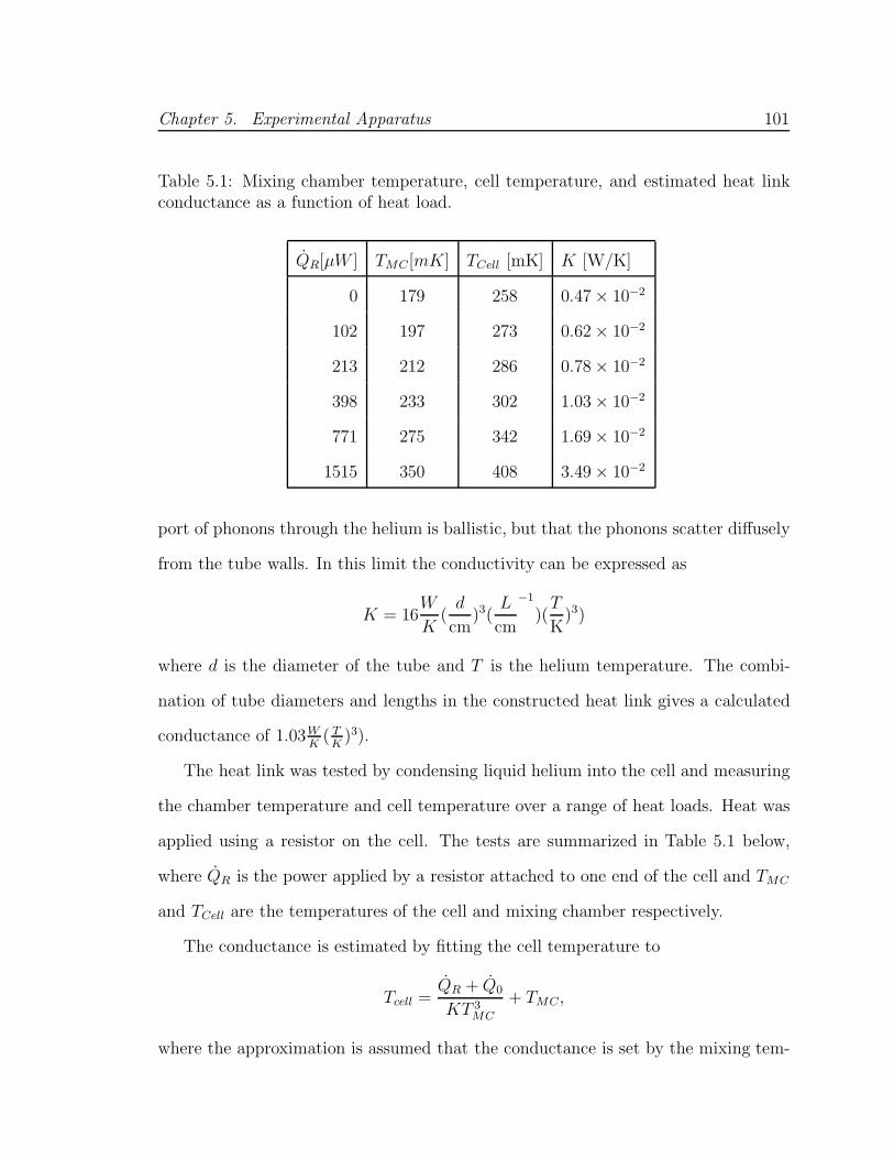
Chapter 5. Experimental Apparatus 101
Table 5.1: Mixing chamber temperature, cell temperature, and estimated heat linkconductance as a function of heat load.
QR[µW ] TMC[mK] TCell [mK] K [W/K]
0 179 258 0.47 × 10⁻²
102 197 273 0.62 × 10⁻²
213 212 286 0.78 × 10⁻²
398 233 302 1.03 × 10⁻²
771 275 342 1.69 × 10⁻²
1515 350 408 3.49 × 10⁻²
port of phonons through the helium is ballistic, but that the phonons scatter diffusely
from the tube walls. In this limit the conductivity can be expressed as
K = 16W
K(
d
cm)3(
L
cm
−1
)(T
K)3)
where d is the diameter of the tube and T is the helium temperature. The combi-
nation of tube diameters and lengths in the constructed heat link gives a calculated
conductance of 1.03WK
( TK
)3).
The heat link was tested by condensing liquid helium into the cell and measuring
the chamber temperature and cell temperature over a range of heat loads. Heat was
applied using a resistor on the cell. The tests are summarized in Table 5.1 below,
where QR is the power applied by a resistor attached to one end of the cell and TMC
and TCell are the temperatures of the cell and mixing chamber respectively.
The conductance is estimated by fitting the cell temperature to
Tcell =QR + Q0
KT 3MC
+ TMC,
where the approximation is assumed that the conductance is set by the mixing tem-

Chapter 5. Experimental Apparatus 102
perature temperature. Here K and Q0 are free parameters. The measured mixing
chamber and cell temperatures and best fit are shown below in Figure 5.6. The best
fit implies a conductance K of 0.81 ± 0.04WK
( TK
)3), with an intrinsic heat load Q0 of
360 µW. This matches the calculated conductance (1.03WK
( TK
)3)) to within 20%.
0.45
0.40
0.35
0.30
0.25
0.20
Cel
l Tem
pera
ture
(K
)
0.400.350.300.250.200.15Mixing Chamber Temperature (K)
Figure 5.6: Conductivity of the superfluid heat link.
By cooling the mixing chamber, gaseous helium introduced through the fill lines
gradually liquifies within the buffer cell and drips down into the experimental cell.
The cell can be filled and cooled to base temperature within 18 hours after condensing
is begun. While cooling, good thermal contact is maintained between the cell and the
mixing chamber, even when the helium is above the λ point. This can be attributed
to convection, since the superfluid is more dense than the normal fluid and cooling
is performed at the top of the system. However, if the mixing chamber is warmed
while the cell is full, it is possible for there to be a large thermal mismatch between
the cell and the mixing chamber, with warm (> 4 K) normal fluid floating above the
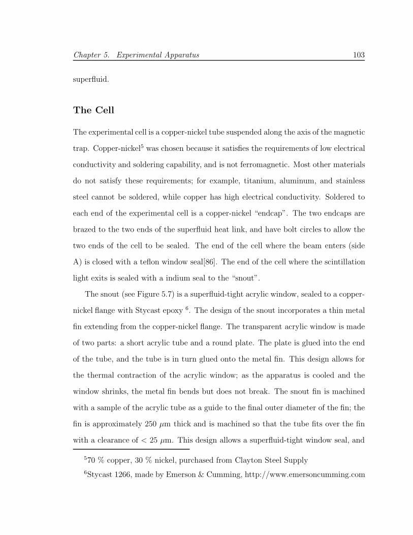
Chapter 5. Experimental Apparatus 103
superfluid.
The Cell
The experimental cell is a copper-nickel tube suspended along the axis of the magnetic
trap. Copper-nickel5 was chosen because it satisfies the requirements of low electrical
conductivity and soldering capability, and is not ferromagnetic. Most other materials
do not satisfy these requirements; for example, titanium, aluminum, and stainless
steel cannot be soldered, while copper has high electrical conductivity. Soldered to
each end of the experimental cell is a copper-nickel “endcap”. The two endcaps are
brazed to the two ends of the superfluid heat link, and have bolt circles to allow the
two ends of the cell to be sealed. The end of the cell where the beam enters (side
A) is closed with a teflon window seal[86]. The end of the cell where the scintillation
light exits is sealed with a indium seal to the “snout”.
The snout (see Figure 5.7) is a superfluid-tight acrylic window, sealed to a copper-
nickel flange with Stycast epoxy 6. The design of the snout incorporates a thin metal
fin extending from the copper-nickel flange. The transparent acrylic window is made
of two parts: a short acrylic tube and a round plate. The plate is glued into the end
of the tube, and the tube is in turn glued onto the metal fin. This design allows for
the thermal contraction of the acrylic window; as the apparatus is cooled and the
window shrinks, the metal fin bends but does not break. The snout fin is machined
with a sample of the acrylic tube as a guide to the final outer diameter of the fin; the
fin is approximately 250 µm thick and is machined so that the tube fits over the fin
with a clearance of < 25 µm. This design allows a superfluid-tight window seal, and
570 % copper, 30 % nickel, purchased from Clayton Steel Supply
6Stycast 1266, made by Emerson & Cumming, http://www.emersoncumming.com

Chapter 5. Experimental Apparatus 104
4K WindowEpoxy Joints
2-4 mm12.5 mm
6 mm
20 mm
Cell Endcap
Snout
Cell Tube
Solder Joint
Indium Seal
250 µm
Figure 5.7: Design of the snout
has proved remarkably leak-free from cool-down to cool-down.
The cell is held in place using Kevlar yarn that wraps around the cell tube and
is held from the IVC (see Figure 5.8). Kevlar is used for this purpose because of its
combination of low thermal conductivity and high tensile strenth. The yarn is made
of 4 twisted threads, each with a diameter of 400 µm. Its thermal conductivity is
3× 10⁻⁴ W cm−2 K−1. The yarn is wrapped around the cell and attached to two “cell
positioning devices”. The cell positioning devices mount to the IVC and can pull the
cell up and down without twisting the Kevlar (see reference [23] for more details).
The cell is prevented from moving in the z direction by additional Kevlar strings (one
at each end of the dewar) connecting the cell to the IVC. The distance between the
cell and the 4 K window is set to be 2 mm. The thermal load on the cell through the
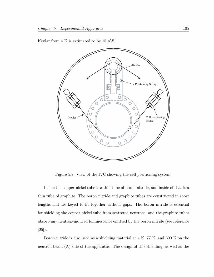
Chapter 5. Experimental Apparatus 105
Kevlar from 4 K is estimated to be 15 µW.
z Positioning String
Kevlar
Kevlar Cell positioning device
Figure 5.8: View of the IVC showing the cell positioning system.
Inside the copper-nickel tube is a thin tube of boron nitride, and inside of that is a
thin tube of graphite. The boron nitride and graphite tubes are constructed in short
lengths and are keyed to fit together without gaps. The boron nitride is essential
for shielding the copper-nickel tube from scattered neutrons, and the graphite tubes
absorb any neutron-induced luminescence emitted by the boron nitride (see reference
[25]).
Boron nitride is also used as a shielding material at 4 K, 77 K, and 300 K on the
neutron beam (A) side of the apparatus. The design of this shielding, as well as the

Chapter 5. Experimental Apparatus 106
vacuum seals and black-body radiation issues pertaining to the A-side windows, are
fully discussed in reference [25].
5.4 The Detection Insert
This section describes the design and calibration of the detection insert used to count
trapped neutrons in August, 2001. The detection insert is based on tetraphenyl
butadiene (TPB) evaporated on a Gore-tex sheet, rolled up into a tube and slid into
the trapping region.
The development of helium scintillation detectors for this experiment is described
in full detail in Chapter 3 of this thesis, and the physical mechanism of the scintilla-
tion is described in Chapers 2 and 4. The great majority (> 80%) of the scintillation
light from singlet decay is emitted within 20 ns of the ionization event. Each neutron
decay event creates a bright flash of EUV light, which is converted to a pulse of blue
light by the wavelength shifter. This visible light is transported to room temperature
through windows and light guides, and is detected by photomultipliers at room tem-
perature. In this way, neutron decays events result in bursts of photoelectrons, which
are detected and recorded electronically.
A sketch of the detection insert and associated optics is shown in Figure 5.9. The
detection insert is located in the center of the trapping region and surrounds the
region where neutrons beta-decay. It is made from two sheets of TPB coated Gore-
tex rolled into tubes and placed end-to-end7, making a tube that is 35 cm long and
8.4 cm in diameter. Each sheet is first cut to a rectangle 17.5 cm x 28 cm in area.
The sheets are then placed in an organic evaporation rig and coated with TPB as
7Unembossed GoreTex GR gasket material, Gore Corporation(www.gorefabrics.com).

Chapter 5. Experimental Apparatus 107
described in Chapter 3. Each sheet required 4 evaporations to achieve a high enough
TPB density, measured by concurrently evaporating TPB onto 2.5 cm x 6.3 cm glass
slides placed in the evaporation rig along with the Gore-tex. The density of TPB on
the Gore-tex is not uniform and is estimated to be between 200 and 400 µg cm−2. The
TPB absorbs EUV light and fluoresces in the blue, with a peak wavelength of 440
nm. Blue photons, after being emitted by the TPB, on average reflect several times
from the TPB coated Gore-tex before escaping out through one of the two tube ends.
Some of the light is absorbed by the TPB coating, which is not a perfect reflector.
The reflectivity and specularity of TPB-coated Gore-Tex has not been measured, and
thus it is difficult to estimate the fraction of blue light emitted by the TPB that
finally escapes the Gore-Tex tube.
200 mK acrylic window
Acrylic light guide
Superconducting magnetic trap
TPB evaporated on Gore-tex
Boron oxide beam dump
Superfluid helium-filled trapping region
Figure 5.9: The neutron detection cell
In order for the TPB luminescence to be collected by light guides and trans-
ported to room temperature, it must pass through an optically transparent, neutron-
absorbing disc of boron oxide located directly after the trapping region. Considerable
effort went into developing a neutron beam dump that was both transparent and free

Chapter 5. Experimental Apparatus 108
of elements that would activate under neutron irradiation. This was desirable because
a transparent beam dump would allow most of the scintillation light through, greatly
improving the detection efficiency of trapped neutron decay events. The three ma-
terials that we considered for transparent beam dumps were lithium fluoride (LiF),
pure boron oxide (B2O3), and a glass fashioned from a melt of B2O3, Li2CO3, and
ZrO2.
Lithium fluoride was initially the most promising of these materials; however it was
found that LiF luminesces very brightly for a considerable time after being irradiated
by neutrons[25]. No other material was found to luminesce as much as LiF; this is
attributable to color center relaxation in the crystalline matrix.
The second approach was undertaken in collaboration with the group of Edgar
Dutra Zanotto in Brazil. High purity powder samples of B2O3, Li2CO3, and ZrO2
were used. After several attempts, a transparent glass (the “Brazilian glass”) that was
stable in atmosphere was produced by the Zanotto group. It consisted of 70% B2O3,
27% Li2CO3, and 3 % ZrO2 by weight8. Each of these compounds was calculated to
yield little activation (< 1 decay s−1) after 30 minutes of neutron acivation. However,
after exposing the Brazilian glass to the neutron beam and monitoring its gamma ray
emission via a germanium counter, it was found that a high flux of 511 keV gamma
rays was emitted. Then, by exposing the glass again to neutrons and placing it in
contact with a piece of plastic scintillator, it was found that the activity decays with
a half-life of 6480 ± 40 s (see Figure 5.10). This identified the activated species as
18F, a β+ emitter with a 6590 second half-life. It is believed that the combination
of lithium and oxygen in the same material brought about the reaction 16O(t, n)18F
following tritium emission by the lithium upon neutron capture. The unexpected,
8Chemicals purchased from Alfa Aesar (www.alfa.com)

Chapter 5. Experimental Apparatus 109
intense positron emission from the Brazilian glass made it unusable for the neutron
trapping experiment.
5000
4000
3000
2000
1000
0
Cou
nts
35x103
302520151050t (s)
Figure 5.10: The positron emission decay curve of the Brazilian glass after 15 minuteexposure to the neutron beam.
The final beam dump was fashioned from a disc of boron oxide, 99.9999% purity9.
The difficulty with boron oxide is that it clouds up when exposed to atmosphere (it is
hygroscopic). However, we found that by minimizing its exposure to the atmosphere,
its transparency could be maintained within acceptable limits. It was polished at
the NIST glass shop, then kept under vacuum until needed. We found that it could
be kept in the atmosphere for up to 15 minutes before clouding significantly (see
Figure 5.11). The boron oxide also lumineseces a bit when exposed to neutrons; this
is believed to be the prime source of luminescence background in the experiment (see
reference [25]).
9Boron oxide disc purchased from All-Chemie Ltd., Mt. Pleasant, SC (843-884-
Chapter 5. Experimental Apparatus 110
100
90
80
70
60
50
40
Tra
nsm
issi
on (
%)
100806040200time (minutes)
Figure 5.11: The transmission of boron oxide as a function of atmospheric exposuretime. This measurement was performed by measured the transmitted light from anLED with a photodiode.
Following the beam dump is a UVT acrylic light guide of diameter 8.7 cm and
length 40.7 cm that transports light from the Gore-Tex tube to the end of the ex-
perimental cell10. The beam dump is held to the light guide with FEP teflon tape11.
The light guide is wrapped in a 175 µm thick layer of Tyvek, a paper that protects
the light guide from scratches and fingerprints and increases its light transport effi-
ciency12. The light guide slides inside the experimental cell, and is surrounded by
tubes of graphite and boron nitride. Three stainless pegs radially extend from the
light guide in the endcap region, and position the light guide within the cell. The
4400) (www.allchemie.thomasregister.com)
10UVT acrylic material purchased from Boedecker Plastics, Shiner, TX(www.boedeker.com). All light guides polished by Universal Plastics, Akron, OH
11McMaster-Carr, New Brunswick, NJ
12Tyvek is a paper made from filaments of polyethylene, made by DuPont.

Chapter 5. Experimental Apparatus 111
pegs are 3 mm diameter, 10 mm long, and are recessed 5 mm deep into lightguide.
The axial position of the pegs is chosen so that the end of the light guide ends up
just inside the snout window.
The optics arrangement used to carry light to room temperature is shown in
Figure 5.12. Scintillation light that passes out of the light guide and through the
snout window must pass through acrylic and quartz windows at 4 K. The acrylic
window makes an indium seal to a flange at 4 K, separates the IVC and OVC, and
absorbs black-body infrared radiation from higher temperatures. Because the thermal
conductivity of the acrylic window is poor, a thin (0.33 mm thick) sheet of quartz
is epoxied to the outer surface of the acrylic window to prevent a hot spot from
developing in the center of the acrylic window. This is critical in minimizing black-
body radiation (see reference [25]). Unfortunately, the quartz cracked quite a bit as
the experiment cooled down; this reduced light transmission.
After the 4 K window is a second light guide, this one of larger diameter (11.4
cm) than the first. This acrylic rod transports scintillation light from 77 K to 300 K,
and is 35 cm long. The 77 K end of the light guide is heat sunk to the 77 K flange
using strips of aluminum foil and has copper wires glued to its end face; this evens
out the temeprature at the end of the light guide and thereby reduces the emission
of blackbody radiation (see reference [25]). The wire pattern covers 11% of the face
of the light guide and therefore reduces light transmission.
A vacuum seal is formed around the second light guide using a Viton O-ring seal.
A metal clamp fastens tightly around the light guide and prevents it from being pulled
into the OVC. The O-ring “UltraTorr” seal and clamp are described more completely
in reference [23] and are sketched in Figure 5.13.
At room temperature, the optics are surrounded by aluminum cans that contain

Chapter 5. Experimental Apparatus 112
Cryogenic cell
4 K acrylic window
Acrylic light guide
PMTs
Aluminized acrylic light splitter
PMT adapter
Figure 5.12: Light collection optics
the photomultiplier tubes. These cans are held together by O-ring seals and can
maintain a positive pressure relative to the guide hall atmosphere. Dry nitrogen is
flowed through the photomultipliers cans to flush out any helium; this precaution is
taken to avoid helium poisoning of the photomultiplier tubes (which causes them to
afterpulse). In normal operation, the scintillation light is split into two photomulti-
pliers by a “light splitter”, which is two light guides glued together at right angles
and aluminized13. The scintillation light then enters the photocathode of the two
photomultiplier tubes. The photomultipliers are coupled to the light guide splitter,
and the light guide splitter coupled to the large light guide, by optical grease14.
The scintillation light is split into two photomultiplier tubes to avoid backgrounds
from dark counts and neutron-induced luminescence. Because time-dependent lu-
13Alumization performed by Evaporated Coatings, Inc., Willow Grove, PA(www.evapcoatings.thomasregister.com)
14RX-6 optical grease purchased from Rexon, Inc., Beachwood, OH(www.rexon.com)

Chapter 5. Experimental Apparatus 113
4 1/2-inchLightpipe
Ring Clamp
positioningscrews
Teflon O-ring
Viton O-rings
Compression Ring
Base
Nut
Figure 5.13: The fitting used to form a vacuum seal around the light guide.
minescence is produced in the boron oxide beam dump following neutron irradia-
tion, special steps must be taken to avoid counting luminescence events as neutron
decays[25]. While we believe that luminescence creates single, uncorrelated photons,
a neutron decay should produce a large, brief pulse of blue light. By requiring that
two PMTs detect a signal in coincidence, luminescence backgrounds should be highly
suppressed. We have found that requiring coincidence is more effective than requiring
a high photoelectron number in a single photomultiplier, since there are occasional
large afterpulses seen following single photoelectron events. While afterpulses are
rare, the large luminescence signal can easily drown out the small expected neutron
decay signal if a single photomultiplier is used.

Chapter 5. Experimental Apparatus 114
Luminescence backgrounds are also reduced by using the photomultiplier model
Burle 8854. As described in Chapter 4, this photomultiplier (like the Burle 8850) has
a high gain GaP second dynode, which gives lower gain dispersion than most other
commercial tubes. Because of this, the number of photoelectrons resulting from a
given event can be determined with high accuracy, and events that result in a low
number of photoelectrons may be easily cut from the data set in off-line analysis. The
dark count spectrum of the Burle 8854 is shown in Figure 5.14.
2500
2000
1500
1000
500
0
Coun
ts
10008006004002000
Pulse height
Figure 5.14: The dark count pulse height spectrum of the Burle 8854 photomultiplier.The peak around channel 200 corresponds to single photoelectron events.
Magnetic Shielding
Because photomultiplier gain and quantum efficiency decrease in a magnetic field, and
the magnetic field from the trap solenoids is large at the position of the photomulti-
plier tubes, careful steps must be taken to magnetically shield the photomultipliers.
Each photomultiplier is surrounded by a tube of µ-metal, and the optics assembly at

Chapter 5. Experimental Apparatus 115
room temperature is surrounded by a large µ-metal “Y”15. Finally, a pair of Helmholtz
coils is placed around the light guide at room temperature to cancel the field from
the pinch coil. When the magnetic trap is on (see next section) and the Helmholtz
coil is tuned to the correct current, the field from the magnetic trap decreases the
quantum efficiency of the photomultipliers by less than 5%. The arrangement of the
magnetic shielding and compensating solenoids is shown in Figure 5.15.
Compensating Solenoid
Mu-metal "Y"
Mu-metal tube
Aluminum photomultiplier housing
Photomultipier base
Figure 5.15: Sketch of the magnetic shielding used to protect the photomultipliersfrom the field generated by the magnetic trap.
15Mu-metal tubes and mu-metal “Y” assembly purchased from Amuneal, Inc. Mu-metal tubes are 1 mm thick, Y is 1.6 mm thick.

Chapter 5. Experimental Apparatus 116
Detector Calibration
The detector was calibrated by placing a 113Sn source in the center of the trapping
region and cooling down the entire experiment. Then, placing a single Burle 8854
photomultiplier at the end of the 77 K light guide, it was found that the 364 keV beta
from the 113Sn source caused an average signal of 10.7 photoelectrons to be detected.
The value of 10.7 photoelectrons was derived by dividing the channel position of the
364 keV beta peak by the channel position of the single photoelectron peak. The
calibration peak is shown in Figure 5.16.
1.0x10⁶
0.8
0.6
0.4
0.2
0.0
Cou
nts
(arb
.)
20p.e.151050Photoelectrons
Peak (10.7 p.e.)
Figure 5.16: The calibration pulse height spectrum, taken with a 113Sn source. Asingle 8854 photomultiplier is connected directly to the 77 K light guide.
A calibration curve (see Figure 5.17) was also taken with a S83006F photomul-
tiplier; this tube has the disadvantage of high gain dispersion and poor single pho-
toelectron resolution, but has higher quantum efficiency than the 8854 (25% instead
of 17% at 440 nm). It displays a correspondingly better peak from the 113Sn source.
Chapter 5. Experimental Apparatus 117
Because this tube does not display a distinct single photoelectron peak, it is more dif-
ficult to estimate the average number of photoelectrons in the peak; however one may
estimate this based on the quoted quantum efficiencies of the 8854 and the S83006F
to be 10.7(25/17) = 15.7 photoelectrons. Despite its higher quantum efficiency, the
S83006F was not used in neutron trapping runs; this is because of the considerable
single-photon luminescence detected following neutron irradiation of the cell. Because
of the poor gain dispersion of the S83006F, luminescence events could be more easily
mistaken for neutron decay events.
The efficiency of the light guide splitter was determined by comparing the peak
channel position with one photomultiplier to the peak channel position with the
splitter installed and two photomultipliers attached. It was found that the light
guide splitter is 94% efficient; that is that 47% of the scintillation signal seen with
one photomultiplier is seen in each of the two photomultipliers when the light guide
splitter is used.
Based on the measured pulse height spectrum, the average detection efficiency for
our apparatus can be calculated using a simple Monte Carlo simulation. This simu-
lation takes into account the neutron recoil spectrum, our simple model of position
dependence, finite “Y” efficiency, and considers the splitting of photons between the
two PMTs to be a Poisson process. The dominant error is the uncertainty in the
position dependence of the detection efficiency. The detection efficiency is estimated
to be 61+8−10 % for a threshold of 2 photoelectrons/PMT.
The efficiency of the optics used to transport light from the trapping region to
the photomultipliers was tested using a 113Sn source and a disc of plastic scintillator.
The source-scintillator combination makes a pulse of light of constant size. By placing
this combination directly against the PMT face, measuring the signal magnitude, and
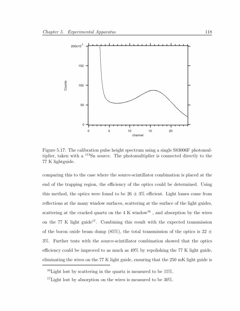
Chapter 5. Experimental Apparatus 118
200x103
150
100
50
0
Cou
nts
20151050channel
Figure 5.17: The calibration pulse height spectrum using a single S83006F photomul-tiplier, taken with a 113Sn source. The photomultiplier is connected directly to the77 K lightguide.
comparing this to the case where the source-scintillator combination is placed at the
end of the trapping region, the efficiency of the optics could be determined. Using
this method, the optics were found to be 26 ± 3% efficient. Light losses come from
reflections at the many window surfaces, scattering at the surface of the light guides,
scattering at the cracked quartz on the 4 K window16 , and absorption by the wires
on the 77 K light guide17. Combining this result with the expected transmission
of the boron oxide beam dump (85%), the total transmission of the optics is 22 ±
3%. Further tests with the source-scintillator combination showed that the optics
efficiency could be improved to as much as 49% by repolishing the 77 K light guide,
eliminating the wires on the 77 K light guide, ensuring that the 250 mK light guide is
16Light lost by scattering in the quartz is measured to be 15%.
17Light lost by absorption on the wires is measured to be 30%.

Chapter 5. Experimental Apparatus 119
close to the snout window, and minimizing the gap between the 77 K light guide and
the 4 K window. Thus, future neutron trapping measurements using this apparatus
should enjoy much higher neutron decay detection efficiencies.
5.5 The Magnetic Trap
This section describes the design and construction of our new superconducting Ioffe
trap. The Ioffe configuration consists of 4 current bars in a quadrupole assembly.
This provides radial confinement, while a pair of pinch coils, each with the same
current sense, provides for axial confinement. See Figure 1.8 for a sketch of the Ioffe
configuration, and Section 1.4 for a description of how magnetic trapping works.
W
Epoxy
Wire
T
H
L
Figure 5.18: The design of a racetrack magnet coil.
A practical way to make the 4 current bars is to use 4 racetrack coils. Each
racetrack coil is made from many turns of a single long strand of superconducting
wire. The preferred superconducting material is niobium titanium, which is super-
conducting below 9.8 K. Along with the length, width, and cross-sectional area of the

Chapter 5. Experimental Apparatus 120
racetrack coils, an important parameter to consider is the wire diameter. A larger
wire diameter implies a larger current supplied to the magnet to achieve a given
current density in the racetrack coil. This current is generally supplied from power
supplies at room temperature, and the necessary cross-sectional area of the current
leads is proportional to the current that must be supplied. Since the heat load on the
helium bath is proportional to the cross-sectional area of the current leads, a lower
current (and thus a smaller diameter wire) helps minimize liquid helium boiloff. On
the other hand, coils designed for smaller wire take longer to wind and quench more
often. A sketch showing the construction of a racetrack coilsis shown in Figure 5.18.
Figure 5.19: A cross-section sketch of the old magnet assembly
The apparatus used to demonstrate magnetic trapping of UCN in May, 1999 used
a magnetic trap with an inner bore of 50 mm, and did not reach its critical current of
400 A, running instead at a maximum current of 180 A, corresponding to a trap depth
of 1.0 T. This magnet is described in more detail in reference [23]. The racetrack coils
were held onto a titanium form, and aluminum spacers were added to the assembly to
make it cylindrical (see Figure 5.19). To keep the assembly together as the coils were
energized, it was compressed by wrapping Kevlar around it under tension, covering
the Kevlar with fiberglass, and then impregnating it with epoxy. Unfortunately,

Chapter 5. Experimental Apparatus 121
it became clear that the Kevlar did not provide enough compression to keep the
coils from moving when they were energized. One one occasion it was noted that
the Kevlar-fiberglass assembly had shifted between cooldowns. It is possible that
the Kevlar creeps over time. It is also known that Kevlar expands slightly at low
temperature, which may have contributed to the lack of compression.
AB
C
Figure 5.20: A cross-section sketch of the new magnet assembly, showing the titaniumform (A) and the two kinds of titanium compressor pieces (B) and (C).
The new magnetic trap was designed to have a larger volume and be demountable.
The chief design change was to use aluminum tubes instead of Kevlar to compress the
assembly. Most of the assembly was built from titanium, which shrinks only 0.141%
as it is cooled to 4 K. Surrounding the assembly with aluminum tubes that fit over the
titanium at room temperature, but shrink 0.41% as they are cooled to 4 K, allowed
compression as the assembly was cooled. The aluminum tubes thus compress the
assembly and preventing the coils from moving as they are energized. The aluminum
could be expected to retain its elasticity from cool-down to cool-down, and the tubes

Chapter 5. Experimental Apparatus 122
could be removed at room temperature. This meant that the assembly could be taken
apart and coils replaced with a minimum of effort.
The new trap was larger than the original and designed to maximize the number
of trapped neutrons. The design was constrained by the size of the helium bath inside
the current dewar. A number of designs were considered, varying coil cross-section,
trap bore, and pinch coil design. The optimal design was determined to have coils
of 2.5 cm x 2.5 cm cross-section, with a bore diameter of 105 mm. With a larger
bore size, a higher detection efficiency could be obtained, as light could be more
easily extracted from the trapping region. Also, the larger trap volume allowed the
confinement of many more neutrons than in with the previous trap.
Figure 5.21: Side view of the titanium magnet form on which the racetrack coils fit.
To calculate the force exerted by the coils as they strain against the aluminum
tubes, consider that the coils push apart with a force determined by their length,
total current, and the magnetic field at the coil.
F = INB�,
where F is the force on one current bar, N is the number of turns of wire in the
current bar, I is the current in the wire, and � is the length of the current bar. The
pressure p exerted by the current bars on the aluminum tubes is then
p =8F
πd�,
and thus
p =8INB
πd.

Chapter 5. Experimental Apparatus 123
With I = 320 A, N = 776.5 on average, B = 3.4 T, and d = 193 mm, one finds that
p = 11.2 MPa.
For a tubular geometry, the pressure exerted by the compression of the aluminum
tube can be determined by
p =2Etδd
d2,
where p is the pressure on the aluminum tube, E is the Young’s modulus of the alu-
minum, t is the thickness of the aluminum tube, δd is the change in diameter of the
aluminum tube, and d is the diameter of the tube. In the case of 6061 aluminum at
low temperature, E = 78.4 GPa. Based on the different expansion coefficients of the
materials used to build the magnet, δd = 240 µm. The diameter d is approximately
193 mm, and the thickness t is 12 mm. Therefore the pressure exerted by the alu-
minum tubes on the magnet assembly is 12.1 MPa. This is more than the pressure
exerted by the coils when fully energized.
Figure 5.22: Sketch of the solenoid assembly
The magnet form and compression pieces were fabricated from grade 2 commer-
cially pure titanium18. The magnet form is 95 cm long, and the two types of com-
pression pieces are 74 cm and 80 cm long. The machining of the titanium was done
18The titanium was purchased from Tico Titanium, New Hudson, MI (248) 446-1995 (www.ticotitanium.com).

Chapter 5. Experimental Apparatus 124
at the McKay machine shop at Harvard, except for the gun-drilling of the central
bore.19
The coils were wound by Bob Michniak and Liang Yang using a new magnet
winding machine at Harvard20. The wire used had a diameter of 740 µm, thinner
than the wire used in the previous magnet21. The coils are each 80 cm long, with a
distance between turnaround centers of 70 cm, and the distance between the centers
of the current bars is 7.0 cm. The coils were wet-wound; epoxy was applied to the coils
as they were wound, with each new layer of wire covered by a new layer of epoxy22.
Each layer took about 30 minutes to wind. The layers of wire were separated by
fiberglass cloth to prevent cracks in the epoxy from propagating. The four coils had
775, 776, 777, and 778 windings, and were protected by G-10 sheets that had been
machined beforehand to cover the faces and sides of the coils. The G-10 sheets thus
provided a flat surface that could be compressed evenly by the aluminum tubes, and
served as well to protect the coils. As the epoxy set overnight after winding, the coil
was compressed to ensure that there were few epoxy-rich regions.
Once the coils were made, they were tested individually. Each of them trained to
within 15% of the 320 A load limit (see Figure 5.23). The training behavior of the
individual coils is shown in Figure 5.24. The coils were then placed on the titanium
form, and the compressor pieces attached. The compressor pieces were bolted tightly
to the form, and then the entire assembly was machined to a uniform diameter of 19.3
19Gundrilling done by Honematic Machine Corp., Boylston, MA (508) 869-2131(www.honematic.com).
20Winding machine model ER1200MP3 from Bobifil (www.bobifil.com).
21Wire used for the new magnetic trap was purchased from Supercon, and had acopper to superconducting ratio of 2:1.
22The epoxy used was Shell Resin 815C with 3140 hardener, at a ratio of 1:1.
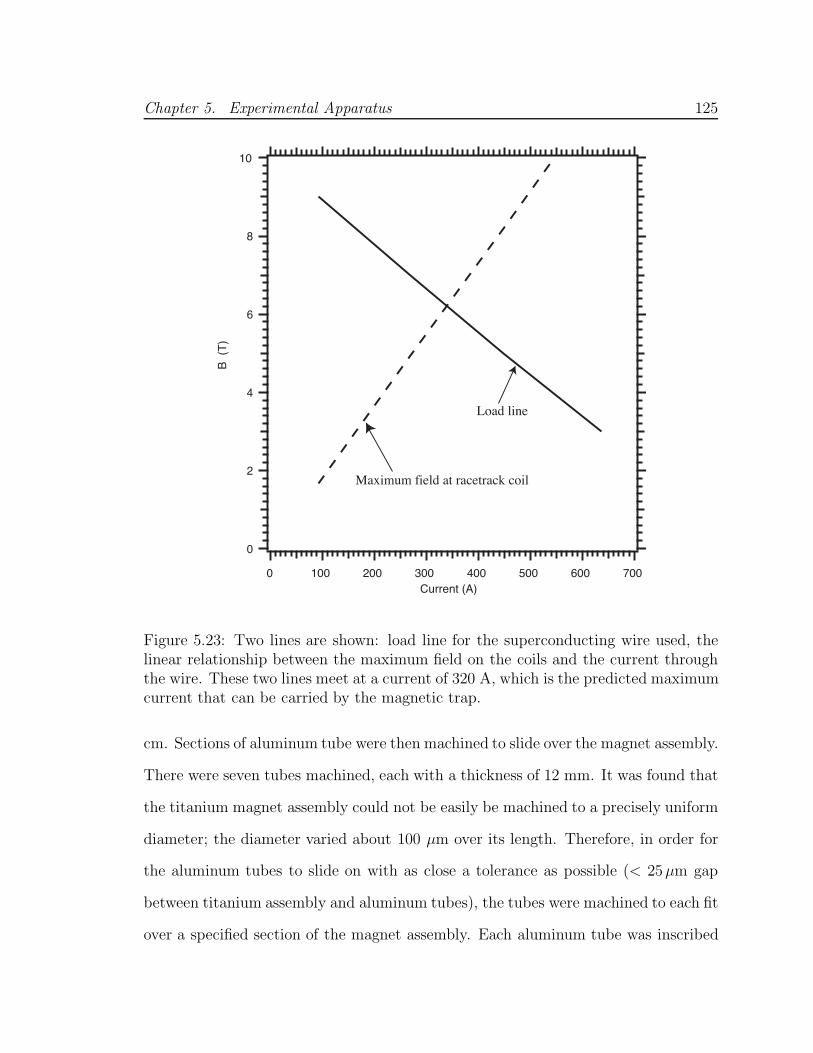
Chapter 5. Experimental Apparatus 125
10
8
6
4
2
0
B (
T)
7006005004003002001000Current (A)
Load line
Maximum field at racetrack coil
Figure 5.23: Two lines are shown: load line for the superconducting wire used, thelinear relationship between the maximum field on the coils and the current throughthe wire. These two lines meet at a current of 320 A, which is the predicted maximumcurrent that can be carried by the magnetic trap.
cm. Sections of aluminum tube were then machined to slide over the magnet assembly.
There were seven tubes machined, each with a thickness of 12 mm. It was found that
the titanium magnet assembly could not be easily be machined to a precisely uniform
diameter; the diameter varied about 100 µm over its length. Therefore, in order for
the aluminum tubes to slide on with as close a tolerance as possible (< 25µm gap
between titanium assembly and aluminum tubes), the tubes were machined to each fit
over a specified section of the magnet assembly. Each aluminum tube was inscribed

Chapter 5. Experimental Apparatus 126
with a numeral from 1 to 7 indicating the order that they should be slid over the
quadrupole assembly.
350
300
250
200
150
100
50
0
Cur
rent
(A
)
87654321Quench number
Coil alpha Coil beta Coil gamma Coil delta
Figure 5.24: The training behavior of the four coils used to build the magnetic trap(denoted alpha, beta, gamma, and delta).
The solenoid assemblies are shown in Figure 5.22. Each assembly has an inner
diameter of 21.4 cm and an outer diameter of 24.6 cm. These dimensions were chosen
so that the entire assembly could fit into the helium bath with a 7 mm clearance.
Within each solenoid assembly there is a “pinch coil” that provides axial confinement
and two “bucking coils” that cause the field from the pinch coil to fall off quickly
versus z. The solenoid forms were wound on the Harvard winding machine as well,
and electrically connected to the quadrupole assembly in series. The whole assembly
was mounted within the helium bath of the main apparatus using techniques similar
to those used in the past (see reference [23]). A cross-section of the full assembly
is shown in Figure 5.25. Current was supplied to the magnetic trap through leads

Chapter 5. Experimental Apparatus 127
running from the top of the dewar23.
Aluminum Compression TubeSolenoid Form
Figure 5.25: Sketch of a cross-section of the magnet assembly.
The magnet assembly was trained multiple times at various months in 2001. Even-
tually the magnet was run at 170 A, after exhibiting excessive training at higher cur-
rents. Details of training behavior are given in reference [25], along with the circuit
used to protect the system from quenches.
23Model L-250 from American Magnetics, Oak Ridge, TNwww.americanmagnetics.com

Chapter 5. Experimental Apparatus 128
The field produced with this trap was studied using the program Biot-Savart24.
This program produces magnetic field profiles along trajectories specified by the user.
Figure 5.26 shows how the magnetic field magnitude varies versus radius. This in-
dicates how the magnetic field increases with radius because of the racetrack coils.
Figure 5.27 shows how the field magnitude varies down the axis of the trap, showing
the axial confinement provided by the two pinch coils. Figure 5.28 shows the field
along a line passing through the turnaround region of the a racetrack coil; this is
the maximum field at any point on the racetrack coil and determines the maximum
current theoretically possible while still maintaining superconductivity. Figure 5.29
shows the field along a line defined by the inner surface of the TPB- coated Gore-tex.
The minimum field on this line determines the magnetic trap depth. The asymmetric
dip in the field is caused by the partial cancellation of the trapping field by the diver-
gent field produces by the pinch coils. Because the pinch coil diameter is relatively
small, the field that it produces is fairly divergent at the trap radius, and this has a
significant effect on the trap depth.
5.6 Background Suppression
Certain kinds of events can mask neutron decays within the trapping region. The
most pernicious of these is gamma ray Compton scattering within the helium bath.
Because Compton scattering transfers gamma ray energy to an electron, it is virtually
indistinguishable from a beta-decay event. And because gamma rays that scatter
in the helium contribute to backgrounds, considerable improvements in statistical
accuracy can be gained by shielding the experiment.
The horizontal section of the experiment is surrounded by lead walls on all sides, 10
24Biot-Savart, Cirrus Software, Inc., Kaleden, BC, Canada.

Chapter 5. Experimental Apparatus 129
1.5
1.0
0.5
0.0
|B| (
T)
-100 -50 0 50 100Radius (mm)
Figure 5.26: Magnetic field magnitude versus radius at z = 0, along a line perpen-dicular to the racetrack coils.
1.4
1.2
1.0
0.8
0.6
0.4
0.2
0.0
|B| (
T)
-600 -400 -200 0 200 400 600
z (mm)
Figure 5.27: Magnetic field magnitude versus z along the central axis of the trap.
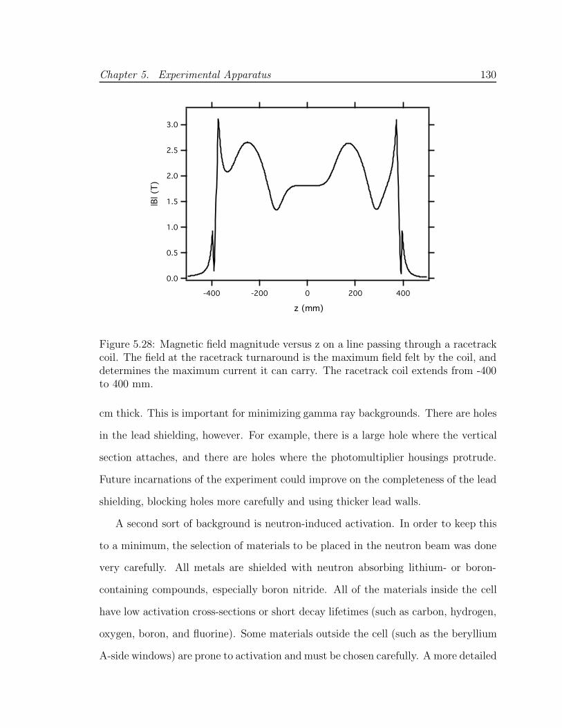
Chapter 5. Experimental Apparatus 130
3.0
2.5
2.0
1.5
1.0
0.5
0.0
|B| (
T)
-400 -200 0 200 400
z (mm)
Figure 5.28: Magnetic field magnitude versus z on a line passing through a racetrackcoil. The field at the racetrack turnaround is the maximum field felt by the coil, anddetermines the maximum current it can carry. The racetrack coil extends from -400to 400 mm.
cm thick. This is important for minimizing gamma ray backgrounds. There are holes
in the lead shielding, however. For example, there is a large hole where the vertical
section attaches, and there are holes where the photomultiplier housings protrude.
Future incarnations of the experiment could improve on the completeness of the lead
shielding, blocking holes more carefully and using thicker lead walls.
A second sort of background is neutron-induced activation. In order to keep this
to a minimum, the selection of materials to be placed in the neutron beam was done
very carefully. All metals are shielded with neutron absorbing lithium- or boron-
containing compounds, especially boron nitride. All of the materials inside the cell
have low activation cross-sections or short decay lifetimes (such as carbon, hydrogen,
oxygen, boron, and fluorine). Some materials outside the cell (such as the beryllium
A-side windows) are prone to activation and must be chosen carefully. A more detailed

Chapter 5. Experimental Apparatus 131
2.0
1.5
1.0
0.5
0.0
|B| (
T)
-600 -400 -200 0 200 400 600
z (mm)
Figure 5.29: Magnetic field magnitude versus z on a line passing along the Gore-textube. This field determines the trap depth.
analysis of activation backgrounds in this experiment can be found in [25].
It has recently been realized that the reaction 10B(α, n)13N is likely to be a sig-
nificant source of time-dependent background. This reaction likely occurs within the
boron nitride shielding material, and was overlooked because it is second-order. The
boron shielding absorbs neutrons via the reaction 10B(n, α)11B, which emits an alpha
of energy 1.48 MeV. But it is then possible for a different boron nucleus to absorb
the alpha particle and emit a neutron, thus producing 13N. This isotope then decays
by positron emission with a lifetime of 863 seconds. Though the cross-section for the
10B(α, n)13N reaction is small (0.02 barns) because of the Coulomb barrier that the α
particle must penetrate to activate 10B, the large number of α particles emitted by the
boron nitride yields an appreciable rate of 13N decays. We estimate that 13N nuclei
are produced in the boron oxide beam dump at a rate of 20 s−1, and a large frac-
tion of the decays deposit energy in the superfluid helium. Like the activation of the

Chapter 5. Experimental Apparatus 132
Brazilian glass, the activation of the boron nitride was unexpected, as second-order
activation processes were not considered in the initial design of the experiment.
A final source of background in this experiment is cosmic ray muons. These are
created by high-energy collisions in the upper atmosphere, and result in a muon
flux at the surface of the Earth of 1 cm−2 min−1. Because the muons pass directly
through the experiment, they can ionize the liquid helium and cause scintillations,
just like neutron beta-decays. But because few of the muons stop in the experiment,
these events can be actively vetoed using slabs of plastic scintillator placed under
experiment. Each muon “paddle” consists of a 2.5 cm x 32 cm x 1.42 m slab of
scintillator, an acrylic condensing region (40 cm long), and a photomultiplier tube.
The muon paddles are wrapped in black cloth to block room light. The muon paddles
are arranged under the experiment as shown in Figure 5.30. By vetoing events that
cause both the 8854’s to trigger and any muon paddle, the constant background level
was reduced by 17 s−1.
5.7 Data Acquisition
The data acquisition system is described in full detail in reference [25] and this section
is meant only as a brief summary. In short, the data acquisition system records
events in which both 8854 photomultipliers looking at the experimental cell fire, and
the muon paddles do not. For each event, the data acquisition system records the
time at which the event occured and the digitized waveforms from the two main
photomultipliers. The data acquisition system is controlled by a Power Macintosh
G3 computer, which also controls the slider and blocker, controls the magnet current,
and turns the photomultipliers on and off at appropriate times during the experiment.
The anodes of the photomultipliers are connected to the inputs of a NIM amplifier,
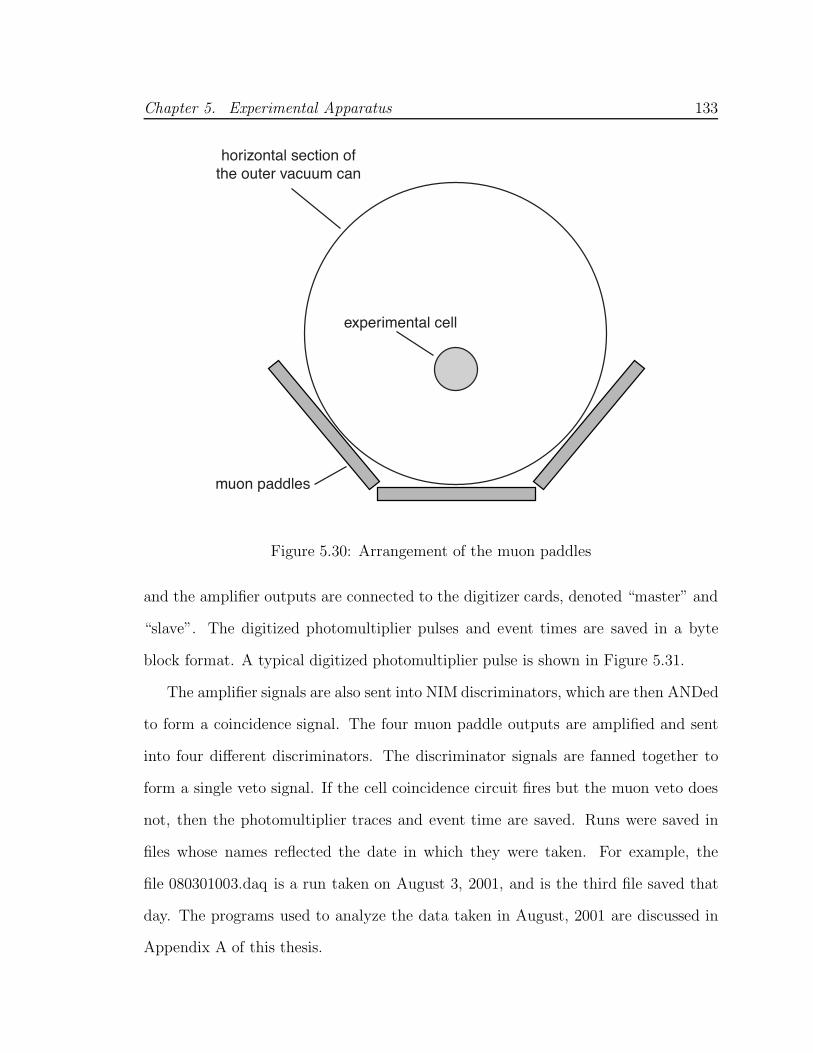
Chapter 5. Experimental Apparatus 133
muon paddles
horizontal section of�the outer vacuum can
experimental cell
Figure 5.30: Arrangement of the muon paddles
and the amplifier outputs are connected to the digitizer cards, denoted “master” and
“slave”. The digitized photomultiplier pulses and event times are saved in a byte
block format. A typical digitized photomultiplier pulse is shown in Figure 5.31.
The amplifier signals are also sent into NIM discriminators, which are then ANDed
to form a coincidence signal. The four muon paddle outputs are amplified and sent
into four different discriminators. The discriminator signals are fanned together to
form a single veto signal. If the cell coincidence circuit fires but the muon veto does
not, then the photomultiplier traces and event time are saved. Runs were saved in
files whose names reflected the date in which they were taken. For example, the
file 080301003.daq is a run taken on August 3, 2001, and is the third file saved that
day. The programs used to analyze the data taken in August, 2001 are discussed in
Appendix A of this thesis.

Chapter 5. Experimental Apparatus 134
250
240
230
220
210
200
190
Val
ue
644832160Point
Figure 5.31: A typical digitized PMT pulse

Chapter 6
Data Analysis
6.1 Data Collection
Data are collected in a series of runs. In each run, neutrons are first loaded into the
trap, and then their decay is observed as a function of time. To load the trap, the
neutron beam is turned on for 2100 s. As shown in Fig. 6.1, the neutron population
in the trap increases monotonically while the neutron beam is on, approaching the
theoretical maximum. Then the beam is turned off and the photomultiplier tubes
are turned on to watch for neutron decays. This period lasts for another 2700 s.
During the beam-off period, the neutrons in the trap decay or are lost from the trap.
Assuming that spurious trap losses are small, the rate of neutron decay detection
should reflect the neutron beta-decay lifetime. After the collection period, a pause of
100 s is observed, and the process is repeated in a new run.
In practice, we perform two sorts of runs, called “positive” and “negative”. In
positive runs, the magnetic field is at its maximum value the entire run. In a negative
run, the magnetic field is off while the neutron beam is on, then raised to its maximum
value just before the beam is turned off, trapping very few neutrons. By subtracting
135

Chapter 6. Data Analysis 136
TimeStart
Beam On
Beam Off
Theoretical Maximum
# tr
appe
d ne
utro
ns
Figure 6.1: A plot of the predicted trapped neutron population versus time.
negative runs from positive runs, backgrounds may be suppressed leaving the neutron
decay signal. The time sequence for positive and negative runs is shown in Figure 6.2.
Each run lasts 4900 s, so ideally 17 runs can be performed per day.
6.2 Data Cuts and Thresholds
In order for an event to be recorded by the data acquisition system, both photomul-
tipliers viewing the detection region must trigger within 20 ns of each other. This
requirement was put in place in order to suppress single-photon backgrounds. There is
a significant rate of uncorrelated photons from neutron-induced luminescence in the
cell; requiring coincidence is highly effective in removing these uncorrelated events
from the collected data. The accidental rate Ra for uncorrelated photons is
Ra = 2R1R2τ,
where τ is the discrimination binwidth created by the triggering electronics, and R1
and R2 are the trigger rates for the two PMTs.
The rate of accidental coincidences is rather uncertain, as our data acquisition
system did not record single photon rates in each photomultiplier. However, a special
measurement of the rate from one of the photomultipliers yielded 19,000 to 11,000

Chapter 6. Data Analysis 137
counts per second between 100 and 600 seconds after the beam was turned off. This
predicts a rate of 4 to 14 s−1, in accord with the measured 1 photoelectron data.
However the accidental coincidence rate at higher thresholds should be much smaller,
as less than 10% of the single photoelectron events are misinterpreted for two pho-
toelectron events (see Figure 5.14). This implies an accidental count rate roughly
100 times smaller for a two-photoelectron threshold, and even lower rates at higher
thresholds. Therefore luminescence backgrounds are not significant for thresholds
higher than two photoelectrons. The requirement of coincidence is critical for cutting
unwanted time-dependent backgrounds.
t [s]axis not linear
0 100 2100 2200 2225 4900
MagnetCurrent
170 A
5 A
PMT Voltage
on
off
BlockerPosition
pass
block
SliderPosition
flight tube
lead
Beam Shutter
open
closed
DataAcquisition
enabled
inhibited
positive
negative
Figure 6.2: Time sequence for data collection.
If the discriminator signals from both PMTs overlap in time, and if none of the
muon paddles trigger, then the event is recorded by the data acquisition system. Both
PMT pulses are digitized and saved, and the time of each event is also recorded. After
a run is finished, the data is saved in a byte block format; each byte block consists of
a series of digitized pulses or a series of time stamps.

Chapter 6. Data Analysis 138
Table 6.1: Threshold as a function of photoelectron number.
Threshold Pulse Area(p.e.)
1 112 303 494 685 876 1067 1258 14410 18212 22015 277
This raw data is converted to a usable form in software, which is described fully
in Appendix I. Simply, each event is characterized by two pulse areas (one for each
PMT), and a time. The pulse area is expressed in terms of photoelectron number
(p.e.) by dividing it by an estimated size of a one-photoelectron pulse (see Table 6.2).
The data is then sorted such that events that are larger than a specified number
of photoelectrons are kept. Only the lower threshold was varied since there are few
events at high thresholds. After sorting, data events from the runs that are being
analyzed (usually a set of runs at a given experimental condition) are histogrammed
to form a single data set for each type of run. The histograms for the positive and
negative sets of runs are subtracted to form a single data set for curve fitting purposes.
The resulting histogram is fit to the function
Ae−kt + B
where t is the time after the neutron beam is turned off. A non-linear, least-squares

Chapter 6. Data Analysis 139
fit is performed using the Igor Pro fitting routine.1
6.3 Backgrounds
The collected data exhibited both time-independent and time-dependent backgrounds,
both of which had significantly larger rates than the expected neutron decay signal.
These backgrounds result largely from ionizing radiation interacting with the helium
bath and light collection optics, and proved to be a significant obstacle to precise
measurement of the neutron decay curve. The measured background rates before
the cell was exposed to neutrons are summarized in Table 6.2. Also shown is the
background rate when the cell is emptied of helium. It can be seen that events in the
helium create the largest fraction of the constant background. This can be explained
by the fact that scattering events in the optics only make Cerenkov radiation, which
is not created in large amounts. Events in the helium, on the other hand, create co-
pious amounts of scintillation light, which is easily detected by the photomultipliers.
Background events are probably largely the result of gamma rays scattering in the
detector. These gamma rays come from long-lived radioactive K, U and Th isotopes
in the apparatus, as well as from prompt neutron capture gammas in the surround-
ing instruments in the guide hall. Other sources might be cosmic rays that miss the
muon paddles, or perhaps radioactive decays in the photomultiplier windows. Made
of glass, the PMT windows contain a significant amount of potassium, and Cerenkov
flashes in one PMT window can be seen by both.
Time-dependent backgrounds are also an issue. In Figure 6.3 the average of the
200 mK positive runs and the average of the 200 mK negative runs are shown, along
1Igor Pro Version 4.04, WaveMetrics, Inc., Lake Oswego, OR,http://www.wavemetrics.com

Chapter 6. Data Analysis 140
Table 6.2: Count rates in coincidence with the detection region empty or full of ultra-pure helium. The rates are tabulated as a function of the lower level threshold numberof photoelectrons required on each PMT. Thus, for a 2 photoelectron threshold, thetotal count rate of events where at least 2 photoelectrons are detected in coincidenceon each PMT is reported. Also shown is the fraction of the background (±0.01) ateach threshold that is from background events in the light collection optics. Notethat these are background rates before subtracting negative runs from positive runs.
Threshold Count rate Count rate Fraction due
(p.e.) Empty [s−1] Full [s−1] to acrylic
1 19.2 30.5 0.63
2 9.3 17.4 0.53
3 5.4 12.5 0.43
4 3.7 9.8 0.38
5 2.7 8.1 0.34
6 2.2 6.9 0.31
7 1.7 6.0 0.29
8 1.4 5.3 0.27
9 1.2 4.7 0.25
10 1.0 4.2 0.24
15 0.5 2.8 0.19
20 0.3 2.1 0.16

Chapter 6. Data Analysis 141
50
40
30
20
10
0
-1 0
Cou
nt r
ate
(s-1
)
25002000150010005000Time after beam off (s)
Average of positives Average of negatives
Figure 6.3: The average positive and average negative runs, with a cell temperatureof 200 mK. Only events with 2 or more photoelectrons detected in each PMT arecounted. The difference is shown below, with error bars.
with the difference between the two. This data is cut at 2 photoelectrons, so any lu-
minescence contribution to the background should be small. Because the background
is clearly time-dependent, there must be activation by the neutron beam. The time-
dependent background is seen at higher thresholds as well; Figure 6.4 shows the same
data cut at 5 photoelectrons. Clearly, activation contributes to the time-dependent
background.
The activation background does not fit well to a single exponential; presumably
this is because there are several species of activated nuclei contributing to the back-
ground. Some suspect nuclei are 20F (half-life 11.0 s), 28Al (half-life 135 s), and 66Cu
(half-life 306 s). Fluorine is present in large amounts in the Gore-tex plastic lining
the cell walls and most likely creates the quickly decaying component seen in both
the 2+ and 5+ data. Aluminum is present in large quantities in the dewar, and cop-

Chapter 6. Data Analysis 142
30
25
20
15
10
5
0
Cou
nt r
ate
(s-1
)
25002000150010005000Time after beam off (s)
Average of positive runs Average of negative runs
Figure 6.4: The average positive and average negative runs, with a cell temperatureof 200 mK. Only events with 5 or more photoelectrons detected in each PMT arecounted. The difference is shown below, with error bars.
per is present in the copper-nickel cell tube. Though the dewar and cell are carefully
shielded from neutrons with boron nitride, the inevitable conclusion is that, somehow,
neutrons managed to activate these materials.
6.4 Data
Data were taken at a variety of temperatures, and in the final set of runs, normal
helium was used instead of ultra-pure 4He. Table 6.3 summarizes the data set. Some
runs were not used in the data analysis; these were excluded for excessive noise or
corrupted data files and comprise about 10% of the total data collected. These runs
are not included in Table 6.3.

Chapter 6. Data Analysis 143
Table 6.3: calendar
Data set Temperature Number of Number of Date range
(mK) positive runs negative runs
“200 mK” 200 - 230 34 36 8/3 - 8/4, 8/6 - 8/9, 8/15 - 8/16
“300 mK” 280 - 330 13 11 8/9 - 8/12,8/18 - 8/19
“400 mK” 400 - 450 14 13 8/6, 8/16 - 8/18
“600 mK” 510 - 640 27 23 8/5 - 8/6
“750 mK” 740 - 760 17 16 8/19 - 8/21
“1 K” 1020 - 1130 19 19 8/12 - 8/15
3He 200 - 250 15 13 8/23 - 8/25
6.5 Analysis
This section contains the fits to all of the aforementioned data sets. In general, it is
seen that the data fits best to a lifetime that is significantly less than the neutron
beta-decay lifetime. The intensity of decays is also less than that expected from the
combination of the theory of the superthermal effect and Monte Carlo simulations[25].
Cold data
For helium temperatures less than 600 mK, upscattering of UCN by phonons in the
superfluid helium is expected to be a small effect[1]. One can thus combine the 200,
300, 400, and 600 mK data sets into a single set. Figure 6.5 shows this data set with
a threshold of 2 photoelectrons, as well as the best fit to this data. The fit lifetime is
482 +85−63 s, considerably shorter than the Particle Data Group (world average) value
of 885.7 ±0.8 s [5] for the neutron beta decay lifetime. This is a 3.0 σ discrepancy.

Chapter 6. Data Analysis 144
Table 6.4: Fit parameters of combined 200-600 mK data as a function of threshold.
Threshold k A B
(photoelectrons) (s−1) (s−1) (s−1)
1 0.0019888 ± 0.000133 3.3087 ± 0.124 0.23434 ± 0.037
2 0.0020741 ± 0.000311 0.95502 ± 0.0834 -0.10295 ± 0.0231
3 0.0023014 ± 0.000369 0.74118 ± 0.0744 -0.077574 ± 0.0174
4 0.0020536 ± 0.000328 0.64586 ± 0.0596 -0.051907 ± 0.0167
5 0.0019743 ± 0.000287 0.58171 ± 0.0473 -0.042303 ± 0.0142
6 0.0019743 ± 0.000287 0.47874 ± 0.0377 -0.031859 ± 0.0129
7 0.0017148 ± 0.000283 0.41711 ± 0.0341 -0.026604 ± 0.0132
8 0.0015738 ± 0.000287 0.36503 ± 0.0304 -0.027543 ± 0.0139
10 0.0014503 ± 0.000319 0.29929 ± 0.0276 0.089566 ± 0.0148
12 0.0014189 ± 0.000396 0.20975 ± 0.024 -0.019046 ± 0.0135
15 0.0017382 ± 0.000571 0.13411 ± 0.022 -0.0089764 ± 0.00835
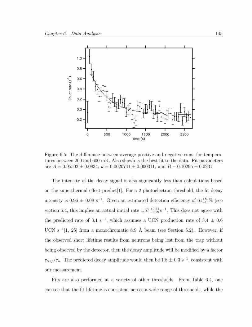
Chapter 6. Data Analysis 145
1.0
0.8
0.6
0.4
0.2
0.0
-0.2
Coun
t ra
te (
s-1)
25002000150010005000time (s)
Figure 6.5: The difference between average positive and negative runs, for tempera-tures between 200 and 600 mK. Also shown is the best fit to the data. Fit parametersare A = 0.95502 ± 0.0834, k = 0.0020741 ± 0.000311, and B − 0.10295 ± 0.0231.
The intensity of the decay signal is also signicantly less than calculations based
on the superthermal effect predict[1]. For a 2 photoelectron threshold, the fit decay
intensity is 0.96 ± 0.08 s−1. Given an estimated detection efficiency of 61+8−10% (see
section 5.4, this implies an actual initial rate 1.57 +0.24−0.29 s−1. This does not agree with
the predicted rate of 3.1 s−1, which assumes a UCN production rate of 3.4 ± 0.6
UCN s−1[1, 25] from a monochromatic 8.9 A beam (see Section 5.2). However, if
the observed short lifetime results from neutrons being lost from the trap without
being observed by the detector, then the decay amplitude will be modified by a factor
τtrap/τn. The predicted decay amplitude would then be 1.8 ± 0.3 s−1, consistent with
our measurement.
Fits are also performed at a variety of other thresholds. From Table 6.4, one
can see that the fit lifetime is consistent across a wide range of thresholds, while the
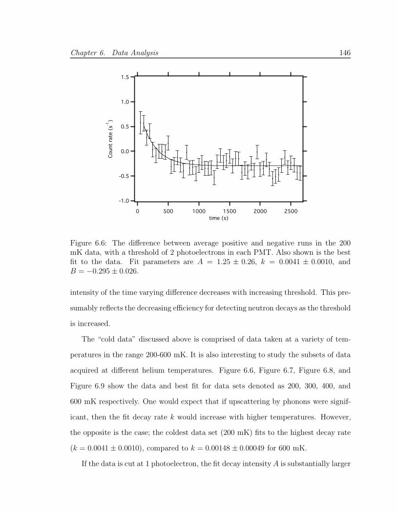
Chapter 6. Data Analysis 146
1.5
1.0
0.5
0.0
-0.5
-1.0
Coun
t ra
te (
s-1)
25002000150010005000time (s)
Figure 6.6: The difference between average positive and negative runs in the 200mK data, with a threshold of 2 photoelectrons in each PMT. Also shown is the bestfit to the data. Fit parameters are A = 1.25 ± 0.26, k = 0.0041 ± 0.0010, andB = −0.295 ± 0.026.
intensity of the time varying difference decreases with increasing threshold. This pre-
sumably reflects the decreasing efficiency for detecting neutron decays as the threshold
is increased.
The “cold data” discussed above is comprised of data taken at a variety of tem-
peratures in the range 200-600 mK. It is also interesting to study the subsets of data
acquired at different helium temperatures. Figure 6.6, Figure 6.7, Figure 6.8, and
Figure 6.9 show the data and best fit for data sets denoted as 200, 300, 400, and
600 mK respectively. One would expect that if upscattering by phonons were signif-
icant, then the fit decay rate k would increase with higher temperatures. However,
the opposite is the case; the coldest data set (200 mK) fits to the highest decay rate
(k = 0.0041 ± 0.0010), compared to k = 0.00148 ± 0.00049 for 600 mK.
If the data is cut at 1 photoelectron, the fit decay intensity A is substantially larger
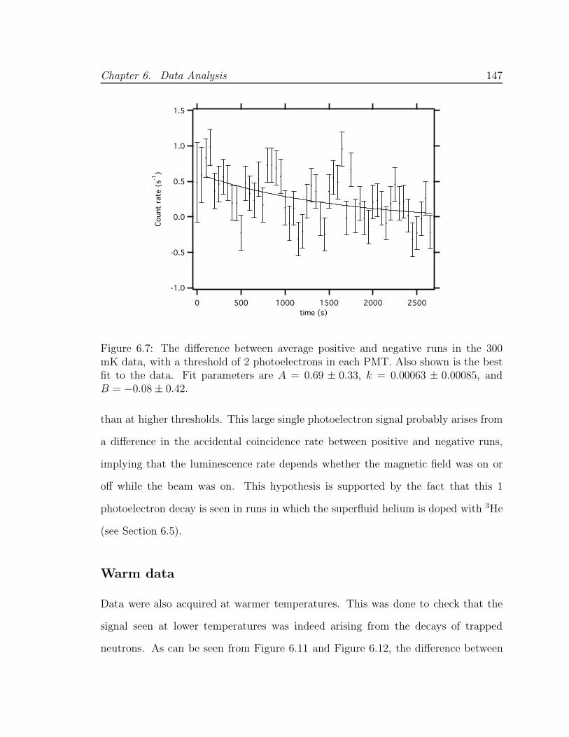
Chapter 6. Data Analysis 147
1.5
1.0
0.5
0.0
-0.5
-1.0
Coun
t ra
te (
s-1)
25002000150010005000time (s)
Figure 6.7: The difference between average positive and negative runs in the 300mK data, with a threshold of 2 photoelectrons in each PMT. Also shown is the bestfit to the data. Fit parameters are A = 0.69 ± 0.33, k = 0.00063 ± 0.00085, andB = −0.08 ± 0.42.
than at higher thresholds. This large single photoelectron signal probably arises from
a difference in the accidental coincidence rate between positive and negative runs,
implying that the luminescence rate depends whether the magnetic field was on or
off while the beam was on. This hypothesis is supported by the fact that this 1
photoelectron decay is seen in runs in which the superfluid helium is doped with 3He
(see Section 6.5).
Warm data
Data were also acquired at warmer temperatures. This was done to check that the
signal seen at lower temperatures was indeed arising from the decays of trapped
neutrons. As can be seen from Figure 6.11 and Figure 6.12, the difference between

Chapter 6. Data Analysis 148
1.5
1.0
0.5
0.0
-0.5
Coun
t ra
te (
s-1)
25002000150010005000time (s)
Figure 6.8: The difference between average positive and negative runs in the 400mK data, with a threshold of 2 photoelectrons in each PMT. Also shown is the bestfit to the data. Fit parameters are A = 1.04 ± 0.13, k = 0.00124 ± 0.00044, andB = −0.09 ± 0.10.
positive and negative runs is suppressed at higher temperatures, as predicted by the
theory of neutron upscattering[1].
3He data
Data were also acquired at a low temperature, but with the isotopically pure 4He
replaced with standard helium from a gas bottle (3He/4He ∼ 10−7, in which neutrons
are captured by the 3He in less than 1 s). Removing the ultra-pure 4He and replacing
it with standard helium took two days, after which the temperature of the cell was
lowered to about 200 mK. Figure 6.15 shows the difference between average positive
and negative “3He runs”. There is no sign of a decay signal in this data. If the decay
rate is fixed to that seen in the 200 mK data (k = 0.0041), the fit decay amplitude
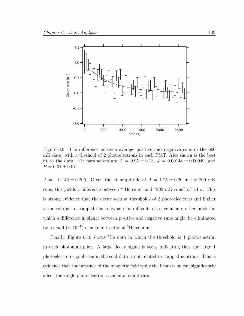
Chapter 6. Data Analysis 149
1.5
1.0
0.5
0.0
-0.5
-1.0
Coun
t ra
te (
s-1)
25002000150010005000time (s)
Figure 6.9: The difference between average positive and negative runs in the 600mK data, with a theshold of 2 photoelectrons in each PMT. Also shown is the bestfit to the data. Fit parameters are A = 0.95 ± 0.13, k = 0.00148 ± 0.00049, andB = 0.01 ± 0.07.
A = −0.146 ± 0.206. Given the fit amplitude of A = 1.25 ± 0.26 in the 200 mK
runs, this yields a difference between “3He runs” and “200 mK runs” of 5.4 σ. This
is strong evidence that the decay seen at thresholds of 2 photoelectrons and higher
is indeed due to trapped neutrons, as it is difficult to arrive at any other model in
which a difference in signal between positive and negative runs might be eliminated
by a small (∼ 10−7) change in fractional 3He content.
Finally, Figure 6.16 shows 3He data in which the threshold is 1 photoelectron
in each photomultiplier. A large decay signal is seen, indicating that the large 1
photoelectron signal seen in the cold data is not related to trapped neutrons. This is
evidence that the presence of the magnetic field while the beam is on can significantly
affect the single-photoelectron accidental count rate.
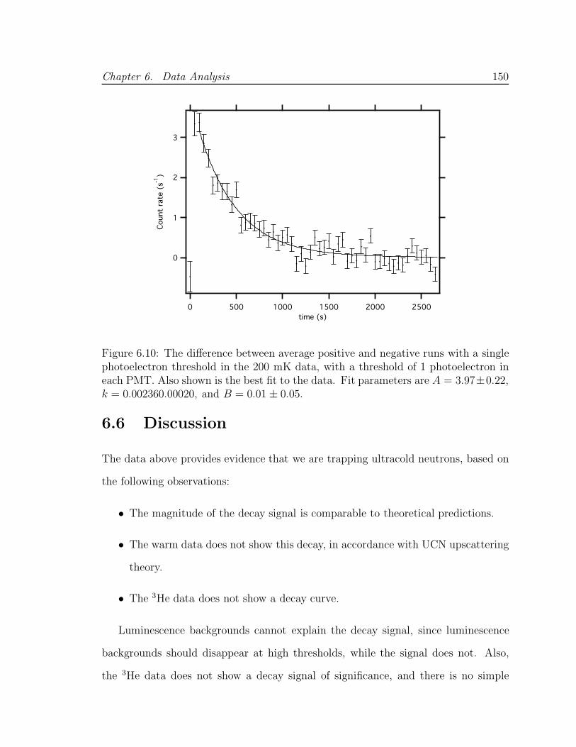
Chapter 6. Data Analysis 150
3
2
1
0
Coun
t ra
te (
s-1)
25002000150010005000time (s)
Figure 6.10: The difference between average positive and negative runs with a singlephotoelectron threshold in the 200 mK data, with a threshold of 1 photoelectron ineach PMT. Also shown is the best fit to the data. Fit parameters are A = 3.97±0.22,k = 0.002360.00020, and B = 0.01 ± 0.05.
6.6 Discussion
The data above provides evidence that we are trapping ultracold neutrons, based on
the following observations:
• The magnitude of the decay signal is comparable to theoretical predictions.
• The warm data does not show this decay, in accordance with UCN upscattering
theory.
• The 3He data does not show a decay curve.
Luminescence backgrounds cannot explain the decay signal, since luminescence
backgrounds should disappear at high thresholds, while the signal does not. Also,
the 3He data does not show a decay signal of significance, and there is no simple

Chapter 6. Data Analysis 151
1.5
1.0
0.5
0.0
-0.5
-1.0
Coun
t ra
te (
s-1)
25002000150010005000time (s)
Figure 6.11: The difference between average positive and negative runs in the 750mK data, with a threshold of 2 photoelectrons in each PMT. Also shown is the bestfit to the data. Fit parameters are A = 0.39 ± 0.16, k = 0.00165 ± 0.00140, andB = −0.03 ± 0.07.
model for why the luminescence signal should depend in any way on the presence of
a small concentration of 3He.
Activation backgrounds can not explain the signal because the signal disappears
in the warm data, and because the signal is not present in the 3He data. There is no
simple model for why an activation signal would depend on temperature changes as
low as 1 K, and no reason to think they would depend on 3He concentration.
The hypothesis that the decay signal is due to trapped neutrons is good at the
5.4 σ level.
The anamolously short lifetime measured in the cold data is puzzling, and remains
to be explained. Possible explanations are:
• Though the subtraction of negative runs from the positive should eliminate
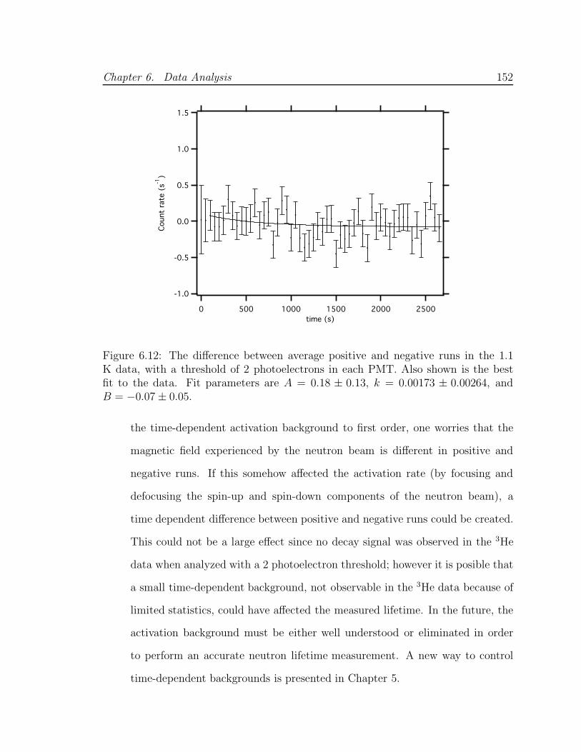
Chapter 6. Data Analysis 152
1.5
1.0
0.5
0.0
-0.5
-1.0
Coun
t ra
te (
s-1)
25002000150010005000time (s)
Figure 6.12: The difference between average positive and negative runs in the 1.1K data, with a threshold of 2 photoelectrons in each PMT. Also shown is the bestfit to the data. Fit parameters are A = 0.18 ± 0.13, k = 0.00173 ± 0.00264, andB = −0.07 ± 0.05.
the time-dependent activation background to first order, one worries that the
magnetic field experienced by the neutron beam is different in positive and
negative runs. If this somehow affected the activation rate (by focusing and
defocusing the spin-up and spin-down components of the neutron beam), a
time dependent difference between positive and negative runs could be created.
This could not be a large effect since no decay signal was observed in the 3He
data when analyzed with a 2 photoelectron threshold; however it is posible that
a small time-dependent background, not observable in the 3He data because of
limited statistics, could have affected the measured lifetime. In the future, the
activation background must be either well understood or eliminated in order
to perform an accurate neutron lifetime measurement. A new way to control
time-dependent backgrounds is presented in Chapter 5.
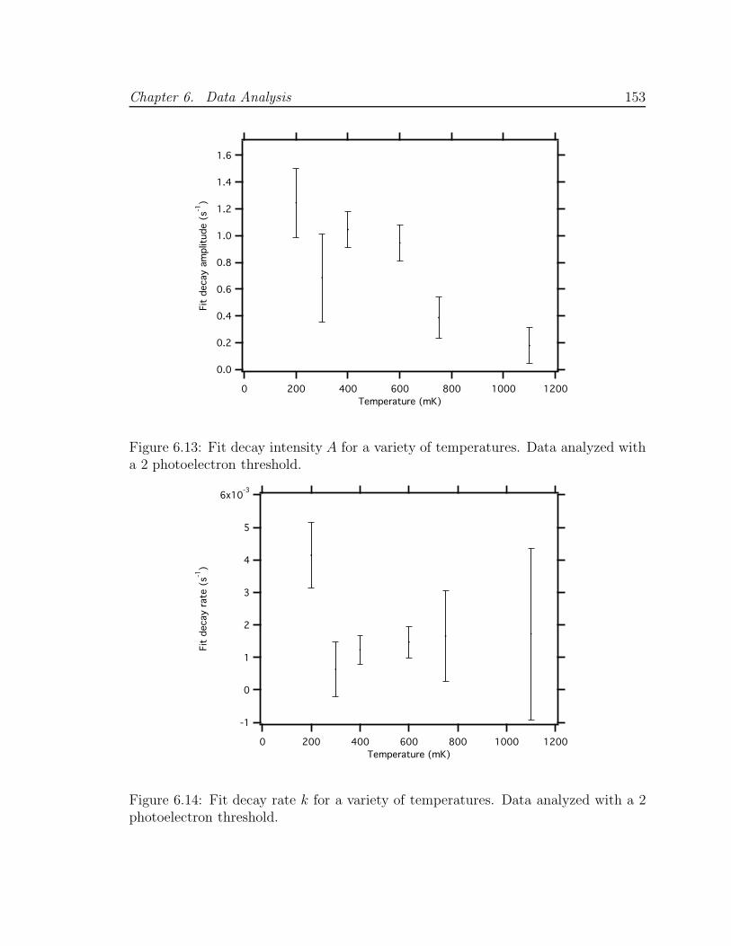
Chapter 6. Data Analysis 153
1.6
1.4
1.2
1.0
0.8
0.6
0.4
0.2
0.0
Fit
deca
y am
plitu
de (
s-1)
120010008006004002000Temperature (mK)
Figure 6.13: Fit decay intensity A for a variety of temperatures. Data analyzed witha 2 photoelectron threshold.
6x10⁻³
5
4
3
2
1
0
-1
Fit
deca
y ra
te (
s-1)
120010008006004002000Temperature (mK)
Figure 6.14: Fit decay rate k for a variety of temperatures. Data analyzed with a 2photoelectron threshold.
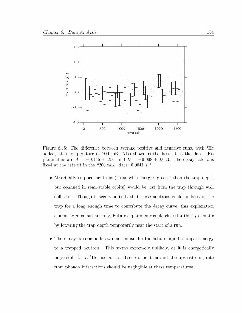
Chapter 6. Data Analysis 154
1.5
1.0
0.5
0.0
-0.5
-1.0
Coun
t ra
te (
s-1)
25002000150010005000time (s)
Figure 6.15: The difference between average positive and negative runs, with 3Headded, at a temperature of 200 mK. Also shown is the best fit to the data. Fitparameters are A = −0.146 ± .206, and B = −0.008 ± 0.033. The decay rate k isfixed at the rate fit in the “200 mK” data: 0.0041 s−1.
• Marginally trapped neutrons (those with energies greater than the trap depth
but confined in semi-stable orbits) would be lost from the trap through wall
collisions. Though it seems unlikely that these neutrons could be kept in the
trap for a long enough time to contribute the decay curve, this explanation
cannot be ruled out entirely. Future experiments could check for this systematic
by lowering the trap depth temporarily near the start of a run.
• There may be some unknown mechanism for the helium liquid to impart energy
to a trapped neutron. This seems extremely unlikely, as it is energetically
impossible for a 4He nucleus to absorb a neutron and the upscattering rate
from phonon interactions should be negligible at these temperatures.
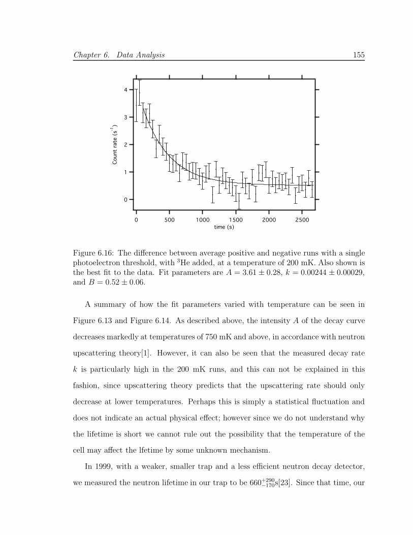
Chapter 6. Data Analysis 155
4
3
2
1
0
Coun
t ra
te (
s-1)
25002000150010005000time (s)
Figure 6.16: The difference between average positive and negative runs with a singlephotoelectron threshold, with 3He added, at a temperature of 200 mK. Also shown isthe best fit to the data. Fit parameters are A = 3.61 ± 0.28, k = 0.00244 ± 0.00029,and B = 0.52 ± 0.06.
A summary of how the fit parameters varied with temperature can be seen in
Figure 6.13 and Figure 6.14. As described above, the intensity A of the decay curve
decreases markedly at temperatures of 750 mK and above, in accordance with neutron
upscattering theory[1]. However, it can also be seen that the measured decay rate
k is particularly high in the 200 mK runs, and this can not be explained in this
fashion, since upscattering theory predicts that the upscattering rate should only
decrease at lower temperatures. Perhaps this is simply a statistical fluctuation and
does not indicate an actual physical effect; however since we do not understand why
the lifetime is short we cannot rule out the possibility that the temperature of the
cell may affect the lfetime by some unknown mechanism.
In 1999, with a weaker, smaller trap and a less efficient neutron decay detector,
we measured the neutron lifetime in our trap to be 660+290−170s[23]. Since that time, our

Chapter 6. Data Analysis 156
statistics have improved markedly, and we can now claim a lifetime of 482 +85−63 s. This
is consistent with our 1999 result, but more clearly demonstrates that the lifetime
we measure in our experiment is signicantly shy of the neutron beta-decay lifetime in
vacuum. Determination of the source of systematic error leading to this discrepancy
is necessary for the future of this technique, and a new apparatus that could be used
to track down the problem is described in the next chapter.

Chapter 7
Conclusions and Recommendations
This thesis has described our method of detecting ultracold neutrons, the detection
cell and its evolution over the history of the experiment, the ultracold neutron trap-
ping apparatus as of Fall 2001, and the analysis of data taken with this apparatus in
August, 2001. The changes to the apparatus undertaken between 1999 and 2001 have
resulted in some significant improvements, while data taken with the new apparatus
have proved informative.
7.1 Progress in Cycle 8
We have again demonstrated the magnetic trapping of ultracold neutrons. Because
our new trap is deeper and larger than the one we used in 1999, and because we
could detect neutron decays with higher efficiency, we are able to assign a higher
significance (5.4 σ) to the hypothesis that we are trapping ultracold neutrons. In
addition, we can point to several recent innovations that should prove invaluable in
future incarnations of this experiment:
• Our new magnetic trap has been reliable, providing a trap depth of 1.1 T and
157
Chapter 7. Conclusions and Recommendations 158
a volume far exceeding that of our previous magnetic trap. Its demountable
design allows coils to be changed if they are damaged, and a protection system
has been built to guard against damaging the magnet in the case of a quench.
• Our detector is more effective, with an efficiency twice that of the 1999 appara-
tus. This is due to a new beam dump technology - capturing the neutron beam
with a transparent, polished window of pure boron oxide.
• Our new superfluid helium heat link has allowed lower cell temperatures. Its
thermal conductance is much higher than our previous copper heat link, and
also does not suffer from eddy current heating. We have had no difficulty in
filling and cooling down the cell through the heat link, and its conductivity
agrees well with theory.
• The development of a 9 A monochromator has improved the prospects for UCN
physics at the NCNR. With a separate beamline at NG6, emitting only 9 A
neutrons, experiments that need this particular wavelength will enjoy lower
backgrounds. Because the monochromator does not interfere with the rest of
the NG6 beamline, the UCN trapping experiment should have greater access to
the beam than in previous years.
7.2 Lessons From Cycle 8
We can also point out several things we have learned from the new upgrade.
• It may be difficult to make a low-current Ioffe trap that is significantly deeper
than the present one. While our new trap displayed excessive training behavior,
the highest current at which we can run is determined by the ability of our

Chapter 7. Conclusions and Recommendations 159
quench protection circuit to absorb energy from the trap. It appears that this
is limited by the high inductance of our coils. Perhaps we could deepen the
trap by winding new coils with larger diameter wire. This would decrease the
inductance of the magnet (since there would be fewer turns in each coil) but
would entail a higher helium boiloff, since higher currents will require larger
current leads.
• Time-dependent backgrounds seem unavoidable with the present apparatus de-
sign. After going to great lengths to minimize the luminescence and activation
backgrounds, we still found that we had significant amounts of both. We are
sensitive to activation because our helium bath is a very effective ionizing radia-
tion detector, with little discrimination between our trapped neutron signal and
backgrounds caused by stray gamma rays, alphas, and betas. Activation back-
grounds can exhibit a multitude of time scales; short-lived decays can obscure
the neutron signal at short times, while long-lived decays change the ambient
background level in our runs. With a background that changes from run to run,
we must fit to the background even when subtracting negative runs. This extra
fit parameter greatly increases the uncertainty in the putative neutron signal.
Luminescence backgrounds are particularly troubling because they can vary in
intensity depending on the history of the magnetic field. Thus, one can not be
sure that time-dependent backgrounds due to luminescence are eliminated by
subtracting field-off runs. Clearly all time-dependent backgrounds must be ei-
ther eliminated or fully understood in order for a neutron lifetime measurement
to be completed.

Chapter 7. Conclusions and Recommendations 160
7.3 Recommendations For Future Work
Separate Production and Detection Regions
Figure 7.1 shows a new concept for the construction of the UCN trapping experiment.
Key to this design is the division of the experiment into two parts: a UCN production
apparatus and a UCN trapping apparatus, connected by a UCN Guide.
The production apparatus would consist of a can filled with superfluid helium,
connected thermally to a dilution refrigerator and surrounded by cryogenic layers at
4 K, 77 K, and 300 K. One end of the can would have a neutron-passing window,
while the rest would be covered by neutron moderating and absorbing materials. The
inside walls of the can would be coated with a material that stores UCN well and has
low wall depolarization, such as beryllium or diamond-like graphite. UCN created
within the superfluid helium by the neutron beam would rattle around in the material
box. The only exit for these UCN would be through a small tube leading out of the
production region (at 90 degrees with respect to the neutron beam), also filled with
superfluid helium. Low-field-seeking neutrons would be prevented from entering the
tube by a solenoid surrounding the tube, a “Magnetic UCN Valve”. High-field-seekers
would be sucked into the field and into a narrow UCN guide.
The walls of the UCN guide need not yield an especially long storage lifetime, but
they do need to have a high UCN potential and should be as specular as possible
(again, beryllium or graphite are appropriate). The UCN guide passes out of the
production apparatus, through a wall of neutron and gamma ray shielding, and into
the UCN trapping apparatus. There the volume increases and the neutrons expand
into the trapping region, also filled with superfluid helium. High field seeking neutrons
would immediately hit the wavelength shifting coating on the walls, upscatter, and

Chapter 7. Conclusions and Recommendations 161
UCN Production Region
MixingChamber
UCN Guide
UCN TrappingRegion
Be foilMagnetic UCN Valve
Magnetic Trap
PMT
UCN Production Apparatus UCN Trapping Apparatus
Shielding
Figure 7.1: A possible future design
be lost.
The procedure for trapping UCN would be as follows: With the magnetic UCN
valve closed (field on) the neutron beam would be turned on and the production
volume filled with UCN. When a suitably high density is reached, the magnetic valve
is opened and the closer pinch coil of the magnetic trap is lowered. Low-field-seeking
neutrons will then pass through the UCN guide and flood the trapping region. Low
energy UCN will not hit the TPB coating because the trapping field prevents them
from reaching it. After a few seconds, the closer pinch coil and magnetic UCN valve
are again closed. A photomultiplier or other light detector, viewing the trap from
above, counts the UCN decays within the trap. After watching the UCN decay, the
cycle is repeated. Note that the neutron beam is on continuously; while neutrons are
being counted in the trap, the production region is being filled with new UCN.
To calculate the wall lifetime of neutrons in the production region, consider a
cylinder 15 cm in diameter, 20 cm long, with a volume Vp of 3500 cm3 and a surface
area Sp of 940 cm2. Then, assuming a UCN velocity v of 400 cm s−1 and a loss per
Chapter 7. Conclusions and Recommendations 162
bounce pp of 8 × 10⁻⁶, one calculates
τ =1
kp
=4Vp
vSppp
= 4650 s.
The value of pp used here is typical of a cold, cleaned beryllium surface, assumes a 2f
value of 2 × 10⁻⁵, and takes into account v/vcrit = 0.38 (see Section 1.3). This wall
lifetime is quite a bit longer than the neutron beta-decay lifetime, so the maximum
UCN density would not be limited by wall losses. Alternately, wall losses could
be significantly worse than assumed here, with little impact on the maximum UCN
density.
After opening the magnetic valve, the loss rate per neutron is
k =v
4Vtotal(Sppp + Sgpg),
where Vtotal is the total volume of production, trap, and guide, Sg is the surface area
of the guide, and pg is the probability of loss per bounce in the guide. Assuming a
Vtrap of 3400 cm3, Vg of 1000 cm3, and pg of 2 × 10⁻⁴, one finds that τ = 260 s. This
means that one would have approximately 260 s to open the magnetic valve, open
the pinch coil, fill the trap with neutrons, and raise the pinch coil. The trap volume
Vtrap of 3400 cm3 corresponds a tube 30 cm long and 12 cm in diameter. The guide is
assumed to be 200 cm long and 2.5 cm in diameter. High specularity of the neutron
guide is desired in this design, as the UCN densities must equalize in the production
and trapping regions before too many UCN are lost. However, a long lifetime in the
UCN guide is likely at low temperatures, and high specularity is possible if the UCN
reflector is coated on an optically flat surface.
One might find it necessary to remove from the experiment the UCN that are not
trapped so as not to introduce any extra backgrounds. This might be done by allowing
the untrapped neutrons to hit an absorbing material after the lower pinch coil has

Chapter 7. Conclusions and Recommendations 163
been ramped up. While loading the trap, this absorbing material would be kept in
a high magnetic field so as not to lose the low-field seeking neutrons. The absorbing
material might double as a UCN detector; for example, a Li:Ti detector could count
each UCN absorbed on its surface. In this way the UCN production from run to
run could be monitored separately from the decay of trapped UCN. A drop in the
rate in the Li:Ti detector would indicate a decrease in the UCN production rate (say,
from a mis-aligned neutron beam or a deteriorating UCN reflection probability in the
production region or UCN guide). A drop in the rate of trapped neutrons detected
relative to the rate in the Li:Ti detector would indicate deteriorating scintillation
detection in the trapping region.
Outside the superfluid helium, the guts of the experiment would be surrounded
by multiple cryogenic layers, at 4 K, 77 K, and 300 K. The Production Apparatus
and Trapping Apparatus would each have their own separate liquid helium and liquid
nitrogen baths, while the UCN guide would have neither, being connected thermally
to the larger halves of the experiment by layers of copper and aluminum at 4K at
77K. The UCN guide and surrounding layers would be only of small diameter: large
enough to pass UCN effectively, yet small enough to pierce lead and polyethylene
layers leaving only a small unshielded area for neutrons and gamma rays to enter
the trapping apparatus. The UCN guide would need a small magnetic field along its
entire length to maintain neutron polarization as they travel; this could be provided
by a weak solenoidal field supplied from room temperature.
An apparatus designed as described would have several advantages over the cur-
rent design, including improved modularity, lower constant background, lower time-
dependent background, higher trapped UCN density, and improved reliability. I will
discuss each of these in turn.

Chapter 7. Conclusions and Recommendations 164
• Improved Modularity. Because the apparatus can be divided into two parts,
each of which can be cooled down separately, experimental work can be done
with each part more easily than if one large, more complicated experiment had
to be cooled down. For example, the UCN production apparatus could be
cooled down to test UCN production rate, UCN material bottle lifetimes, and
the temperature dependence of UCN loss rate in helium. These experiments
could be done by attaching a material at the end of the UCN guide that absorbs
neutrons directly and creates an electronic signal. After building up low field
seekers in the trap, the magnetic valve could be opened, letting the neutrons
be absorbed in the detector. The signal to noise in the detector would be very
high, allowing highly accurate measurements of the UCN production and loss
rates. The UCN trapping apparatus could be tested independently (perhaps at
a remote location if this is convenient) to test the magnetic trap and calibrate
the neutron detector. It will also be easier to get the apparatus leak tight, as
each half of the experiment could be cooled down separately to check for leaks.
Even after the two halves are connected, leaks will be easier to locate because
the two halves of the experiment are well physically separated, each with its
own liquid helium and liquid nitrogen baths. The UCN production apparatus
might later be used as a general UCN source for other experiments, for example
to test experimental concepts for the neutron EDM measurement.
• Lower Constant Background. The UCN trapping apparatus could be more
easily shielded from gamma rays and neutrons than our current apparatus. This
is because there only needs to be a small (15 cm diameter) hole in the shielding to
allow the UCN guide to connect the two halves of the experiment. Because the
UCN trapping apparatus does not need to be close to the beam aperture, there
Chapter 7. Conclusions and Recommendations 165
will be more room for thicker and more complete neutron and gamma shielding.
The muon rate in a vertical trap is lower than in a horizontal trap because the
cosmic ray flux is peaked in the downward direction. Also, cosmic rays that
do pass through the detector will be more easily detected, as a smaller muon
paddle area coverage will be necessary. One new source of constant background
would be VCN from the production region that travel through the guide and
decay in the trapping region. The magnitude of this background is uncertain
and must be tested experimentally; however it is unlikely to be large compared
to the background from gamma rays.
• Lower Time Dependent Backgrounds. In the current apparatus, signifi-
cant time dependent backgrounds are apparent after the neutron beam is turned
off. The subsequent luminescence and radioactive decay from neutron activation
can obscure the decay signal from trapped neutrons and introduce systematic
error in the measurement of the neutron lifetime. With wide separation be-
tween the UCN production and trapping regions, both of these sources of time
dependent background can be eliminated. Luminescence light from the produc-
tion region can be blocked by baffles and is very unlikely to reach the detector.
Gamma rays from neutron activation are also unlikely to reach the detector, as
the trapping apparatus can be well shielded and is far away from the production
apparatus. Especially tantalizing is the possibility that the neutron beam could
be kept on continuously in this configuration, resulting in total elimination of
time-dependent luminescence and activation backgrounds. This could be done
provided that the constant background coming from the neutron beam is low
enough. This is a plausible scenario considering that our current apparatus
runs with other experiments nearby. There would be a small background from

Chapter 7. Conclusions and Recommendations 166
high-field-seeking UCN that decay in the trapping region, but this should be
small compared to both the signal and the constant background, since most
high field seekers will be upscattered from the walls of the Transport Region
or the trapping region. The capture of upscattered UCN in the surrounding
neutron shielding is unlikely to produce a signal in the superfluid helium.
• Higher UCN Density. With a dedicated UCN production apparatus, this
half of the experiment can be designed to better maximize UCN creation, with-
out the constraints imposed by the bulky magnetic trap. For example, the
production region can be closer to the beam aperture, with fewer, wider colli-
maters. This could double the UCN production. Also, the production region
could be surrounded by a hydrogenous material to reflect neutrons back into
the production region. This method of increasing UCN production has been
studied by Bangert et al.[88]; they find that UCN production can be increased
by a factor of 2 by surrounding the production region with 2 cm of acrylic.
Finally, if the neutron beam is on continuously, the experiment will not have to
pause data collection for a lengthy period of time to accumulate UCN. While
trapped neutrons are decaying and being counted in the Trapping Apparatus,
the production apparatus will be accumulating low field seeking UCN for the
next trapping run. This will yield a higher number of runs per day, with better
statistics as a result. Though the density of neutrons will decrease after the mag-
netic valve is opened by the ratio Vp/(Vt +Vg +Vp), where Vp, Vt, and Vg are the
volumes of the production region, trapping region, and UCN guide respectively,
this ratio should be close to 1 if the production volume is sufficiently large. Also,
some low-field-seekers will be lost to upscattering at surfaces, though ultra-high
vacuum conditions and clean surfaces in the production region should keep these
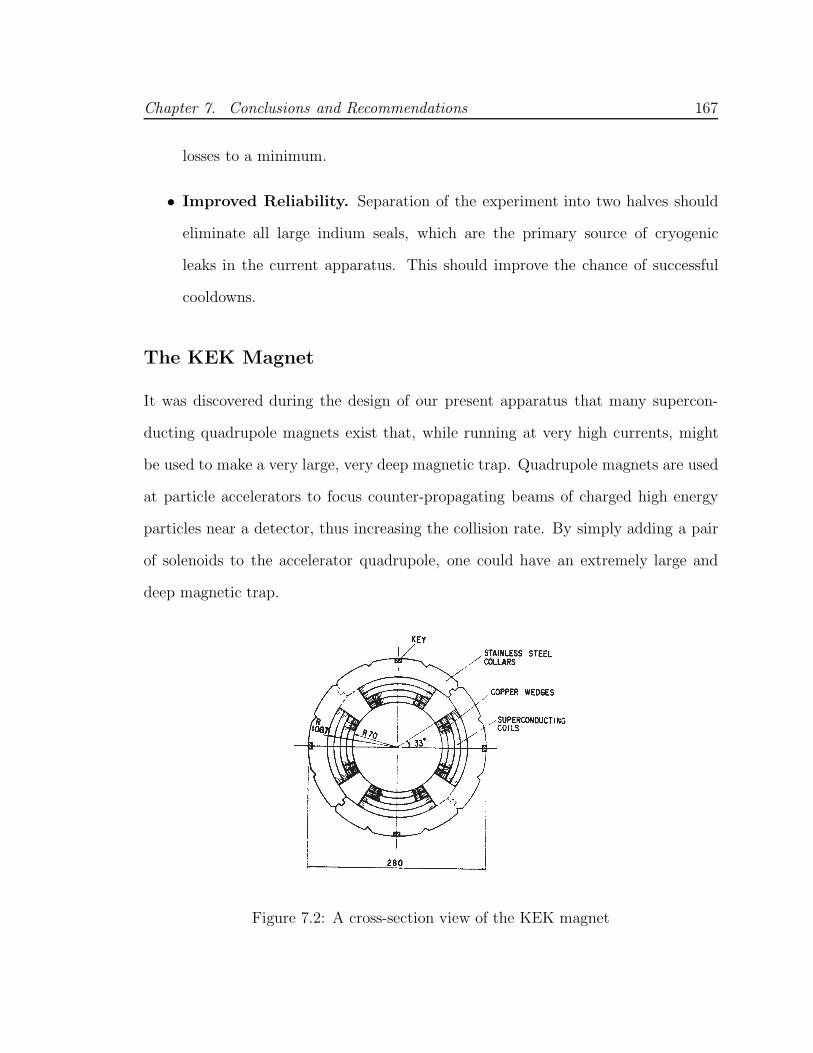
Chapter 7. Conclusions and Recommendations 167
losses to a minimum.
• Improved Reliability. Separation of the experiment into two halves should
eliminate all large indium seals, which are the primary source of cryogenic
leaks in the current apparatus. This should improve the chance of successful
cooldowns.
The KEK Magnet
It was discovered during the design of our present apparatus that many supercon-
ducting quadrupole magnets exist that, while running at very high currents, might
be used to make a very large, very deep magnetic trap. Quadrupole magnets are used
at particle accelerators to focus counter-propagating beams of charged high energy
particles near a detector, thus increasing the collision rate. By simply adding a pair
of solenoids to the accelerator quadrupole, one could have an extremely large and
deep magnetic trap.
Figure 7.2: A cross-section view of the KEK magnet

Chapter 7. Conclusions and Recommendations 168
The most promising magnet design was identified to be the quadrupole magnet
used at the TRISTAN accelerator at KEK in Japan[89]. These magnets are quite
large, sporting a bore diameter of 14 cm, a usable field region 100 cm long, and a
field at the bore wall of 10.0 T when running at 5000 A in superfluid helium[90]. The
load line characteristics of the magnetic are shown in Figure 7.3. These quadrupole
magnets have not been in use since the shutdown of TRISTAN in 1995, and have
been in storage since that time. Excited about the possibility of using one of these
magnets in the neutron trapping experiment, we contacted the group that built and
tested these magnets. The KEK graciously agreed to send us one of their magnets for
testing. We have not yet tested it in conjunction with a solenoidal field, although we
have tested our quench protection circuitry in conjuction with the magnet at currents
as high as 1800 A. There is little doubt whether the magnet would perform well by
itself; the major experimental question is whether the magnet could function properly
under the additional mechanical stresses caused by a superimposed solenoidal field.
The solenoid field would also lower the maximum current. We estimate that a trap
depth of 4.4 T at 4400 A is possible in superfluid helium, given a trap diameter of 10
cm. If the magnet were run at 4.5 K, the maximum trap depth would be about 3.8
T, running at 3800 A.
Incorporating the KEK magnet into our experiment would be a major undertak-
ing. The magnet is quite heavy (400 kg) and large (28 cm diameter, 145 cm length).
With solenoids added, the total diameter of the magnet assembly would be about
35 cm. In addition, it would run on large currents and would thus need quite thick
current leads, generating large heat loads on the helium bath. An estimate for the
heat load from suitable High-Tc leads was provided to us by a manufacturer of such
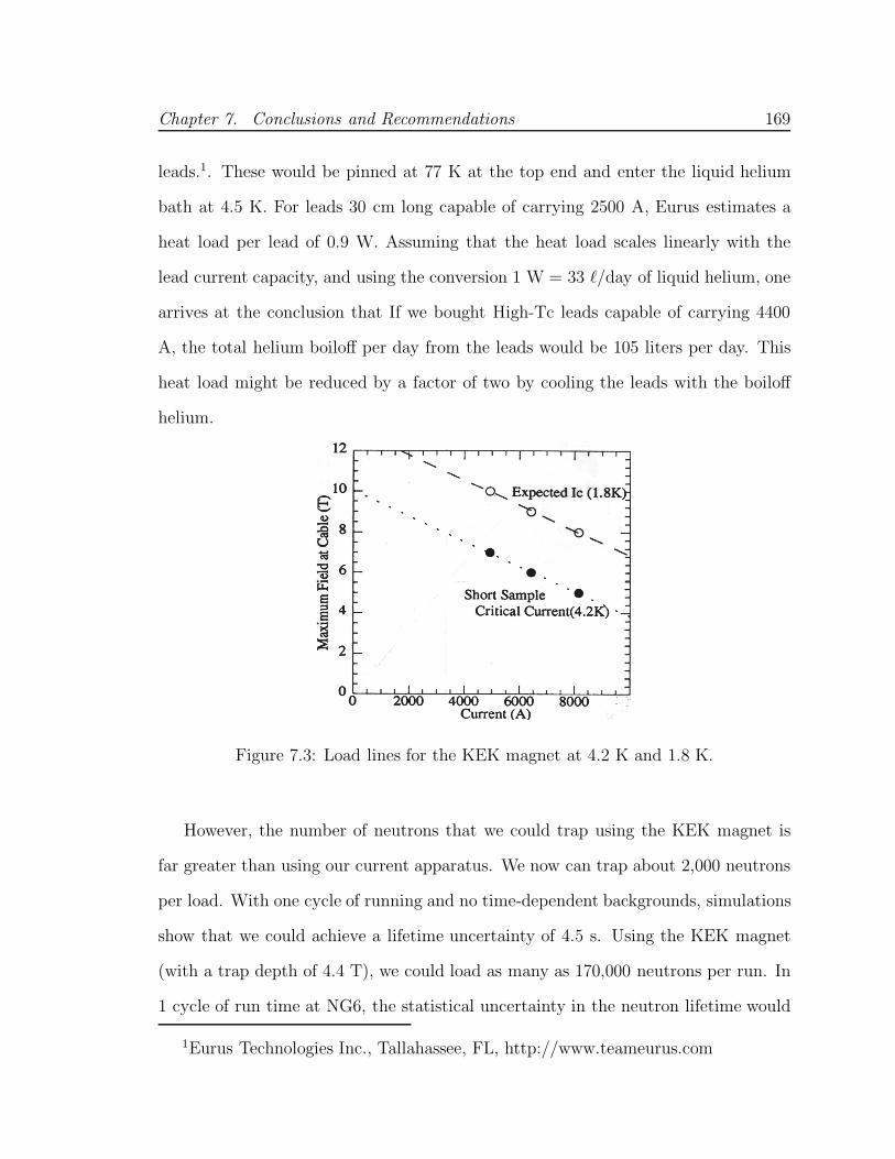
Chapter 7. Conclusions and Recommendations 169
leads.1. These would be pinned at 77 K at the top end and enter the liquid helium
bath at 4.5 K. For leads 30 cm long capable of carrying 2500 A, Eurus estimates a
heat load per lead of 0.9 W. Assuming that the heat load scales linearly with the
lead current capacity, and using the conversion 1 W = 33 �/day of liquid helium, one
arrives at the conclusion that If we bought High-Tc leads capable of carrying 4400
A, the total helium boiloff per day from the leads would be 105 liters per day. This
heat load might be reduced by a factor of two by cooling the leads with the boiloff
helium.
Figure 7.3: Load lines for the KEK magnet at 4.2 K and 1.8 K.
However, the number of neutrons that we could trap using the KEK magnet is
far greater than using our current apparatus. We now can trap about 2,000 neutrons
per load. With one cycle of running and no time-dependent backgrounds, simulations
show that we could achieve a lifetime uncertainty of 4.5 s. Using the KEK magnet
(with a trap depth of 4.4 T), we could load as many as 170,000 neutrons per run. In
1 cycle of run time at NG6, the statistical uncertainty in the neutron lifetime would
1Eurus Technologies Inc., Tallahassee, FL, http://www.teameurus.com

Chapter 7. Conclusions and Recommendations 170
be 0.2 seconds. A larger and deeper trap is necessary for this experiment to reach its
ultimate precision.
While it is unlikely that we would use the KEK magnet in the near future, it is
important that we keep the KEK magnet in mind when we redesign our apparatus.
If we switch to a two-dewar scheme as recommended in this thesis, then the dewar
containing the magnetic trap should be large enough to hold the KEK magnet and
solenoids.
Summary of Recommendations
In summary, we recommend that the design of the neutron trapping apparatus be
changed to allow separate detection and trapping regions. This will require devel-
opment of expertise in our group in the storing of neutrons using material bottles.
It will also require a major effort in the construction of new dewars and associated
cryogenics. We also recommend the winding of new, higher current coils for the mag-
netic trap that we presently use, but constructing the new dewar in such a way that
it could accomodate the much larger KEK magnet.
Appendix A
Data Analysis Software
The software described in this Appendix was used to perform an independent analysis
of the data acquired during August, 2001. It is in many ways similar to the software
developed previously by Carlo Mattoni[25], and serves the same functions. However,
it was written in a short time period after all of the data was collected and was
developed independently. It takes as input the digitized photomultiplier pulses and
time stamps associated with each data run, and outputs a decay curve, given such
parameters as photomultiplier thresholds and specific runs to be analyzed.
There are four separate routines, called the “parser”, the “viewer”, the “cutter”,
and the “histogrammer”. They form a software package called “Danalyzer”. The
individual routines are described below:
• The Parser
The parser takes as input the .daq files that are saved following each data run.
These files contain digitized photomultiplier pulses and time stamps, saved in
a byte block format. Each pulse is read into the program and integrated to
yield a pulse area, which is representative of the total charge collected by the
photomultiplier anode. Each event is then characterized by two pulse areas (one
171
Appendix A. Data Analysis Software 172
for each PMT) and a event time. This information is saved as a .par file.
• The Viewer
The viewer allows the user to see individual photomultiplier traces, compare the
traces of master and slave cards, and study how the parsing algorithm operates.
The viewer takes as input a .daq file, creates a .vie file, and uses this file in its
running procedure.
• The Cutter
The cutter takes as input the .par file outputted by the parser. It allows the
user to eliminate events that do match a combination of designated criteria.
Usually these criteria are pulse size thresholds. The cutter outputs a .cut file.
• The Histogrammer
The histogrammer takes as input the .cut files from a number of user-designated
files, and creates a summed histogram of their decay curves. “Negative” fiels are
subtracted from “positive” files (see Chapter 6) to make a decay curve suitble
for fitting.

Bibliography
[1] R. Golub, D. Richardson, and S. K. Lamoreaux. Ultra-Cold Neutrons. AdamHilger, 1991.
[2] R. E. Lopez and M. E. Turner. Precision prediction for the big-bang abundanceof primordial helium 4. Physical Review D, 59:103502, 1999.
[3] Y. Hayato et al. Search for proton decay through p − > antineutrino K+ in alarge water cerenkov detector. Physical Review Letters, 83:1529, 1999.
[4] D. Dubbers. Particle physics with cold neutrons. Progress in Particle and NuclearPhysics, 26:173–252, 1991.
[5] D.E. Green et al. Particle listings. The European Physics Journal C, 15:1, 2000.
[6] J. Reich et al. A measurement of the beta asymmetry in neutron decay withPERKEO II. Nuclear Instruments and Methods in Physics research A, 440:535–538, 2000.
[7] P. Liaud et al. The measurement of the beta asymmetry in the decay of polarizedneutrons. Nuclear Physics A, 407:53, 1997.
[8] B. G. Erozolimsky et al. Corrigendum: Corrected value of the beta-emissionasymmmetry in the decay of polarized neutrons measured in 1990. Physics Let-ters B, 412:240, 1997.
[9] P. Bopp et al. Beta-decay asymmetry of the neutron and ga/gv. Physics ReviewLetters, 56:919, 1986.
[10] D. Wilkinson. Analysis of neutron beta-decay. Nuclear Physics A, 377:472, 1982.
[11] J. P. Alexander et al. First measurement of the b → π�ν and b → ρ(ω)�νbranching fractions. Physics Review Letters, 77:5000–5004, 1996.
[12] H. Leutwyler and M. Roos. Determination of the elements vud and vus of thekobayashi-maskawa matrix. Zeitschrift fur Physik C, 25:91, 1984.
173
Bibliography 174
[13] S. Arzumanov et al. Neutron lifetime measured by monitored storing of ultracoldneutrons. Nuclear Instruments and Methods A, 440:511–516, 2000.
[14] J. Byrne, P. G. Dawber, C. G. Habeck, S. J. Smidt, J. A. Spain, and A. P.Williams. A revised value for the neutron lifetime measured using a penningtrap. Europhysics Letters, 33:187–192, 1996.
[15] W. Mampe, L. N. Bondarenko, V. I. Morozov, Yu. N. Panin, and A. I. Fomin.Measuring neutron lifetime by storing ultracold neutrons and detecting inelasti-cally scattered neutrons. JETP Letters, 57:82–87, 1993.
[16] V. V. Nesvizhevskiı, A. P. Serebrov, R. R. Tal’daev, A. G. Kharitonov, V. P.Alfimenkov, A. V. Streikov, and V. N. Shvetsov. Measurement of the neutronlifetime in a gravitational trap and analysis of experimental errors. Soviet PhysicsJETP, 75:405–412, 1992.
[17] W. Mampe et al. Neutron lifetime measured with stored ultracold neutrons.Physical Review Letters, 63:593, 1993.
[18] P. E. Spivak. Neutron lifetime obtained from atomic-energy-institute experimentJETP Lett.28, 303(1978). Soviet Physics JETP, 67:1735–1740, 1988.
[19] W. Paul, F. Anton, L. Paul, S. Paul, and W. Mampe. Measurement of theneutron lifetime in a magnetic storage ring. Zeitschrift fur Physik C, Particlesand Fields, 45:25–30, 1989.
[20] J. Byrne, P. G. Dawber, J. A. Spain, A. P. Williams, M. S. Dewey, D. M.Gilliam, G. L. Greene, G. P. Lamaze, R. D. Scott, J. Pauwels, R. Eykens, andA. Lamberty. Measurement of the neutron lifetime by counting trapped protons.Physical Review Letters, 65:289–292, 1990.
[21] M.G.D. van der Grinten et al. Characterization and development of diamond-likecarbon coatings for storing ultracold neutrons. Nuclear Instruments and Methodsin Physics Research A, 423:421–427, 1999.
[22] J. M. Doyle and S. K. Lamoreaux. On measuring the neutron beta-decay lifetimeusing ultracold neutrons produced and stored in a superfluid-4he-filled magnetictrap. Europhysics Letters, 26:253–258, 1994.
[23] C. R. Brome. Magnetic Trapping of Ultracold Neutrons. PhD thesis, HarvardUniversity, 2000.
[24] A. Steyerl and S.S. Malik. Sources of ultracold neutrons. Nuclear Instrumentsand Methods in Physics Research A, 284:200–207, 1989.

Bibliography 175
[25] C. E. H. Mattoni. Magnetic Trapping of Ultracold Neutrons Produced Using aMonochromatic Cold Neutron Beam. PhD thesis, Harvard University, 2002.
[26] P.C. Hendry and P.V.E. McClintock. Continuous flow apparatus for preparingisotopically pure 4He. Cryogenics, 27:131–138, 1987.
[27] H. Fleishman et al. Review of Scientific Instruments, 30:1130, 1959.
[28] E. H. Thorndike and W. J. Shlaer. Review of Scientific Instruments, 30:838,1959.
[29] J.R. Kane and R. T. Siegel. Bulletin of the American Physical Society, 10:515,1965.
[30] J. E. Simmons and R. B. Perkins. Liquid helium scintillation counter as a neutronpolarimeter. Review of Scientific Instruments, 32:1173, 1961.
[31] F. E. Moss and F. L. Hereford. Inhibition of the scintillation of He II. PhysicalReview Letters, 11:63–64, 1963.
[32] F. L. Hereford and F. E. Moss. Recombination luminescence in the scintillationof normal and superfluid liquid helium. Physical Review, 141:204–208, 1966.
[33] J. Jortner et al. Energy transfer phenomena in liquid helium. Physical ReviewLetters, 12:415–416, 1964.
[34] C. M. Surko and F. Reif. Investigation of a new kind of energetic neutral exci-tation in superfluid helium. Physical Review, 175:229–241, 1968.
[35] G. W. Rayfield. Modulation of the neutral excitation current in liquid heliumby electric fields. Physical Review Letters, 23:687, 1969.
[36] R. P. Mitchell and G. W. Rayfield. Neutral excitations from a tritium sourceimmersed in he II. Physics Letters A, 37:231–232, 1972.
[37] W. S. Dennis et al. Spectroscopic identification of excited atomic and molecularstates in electron-bombarded liquid helium. Physical Review Letters, 23:1083–1086, 1969.
[38] A. V. Konovalov and G. V. Shlyapnikov. Decay kinetics of triplet He(23S) exci-tations in liquid and solid helium. Soviet Physics JETP, 73:286–291, 1991.
[39] J. W. Keto et al. Dynamics of atomic and molecular metastable states producedin electron-bombarded superfluid helium. Physical Review Letters, 28:792–795,1972.
Bibliography 176
[40] J. W. Keto et al. Dynamic properties of neutral excitations produced in electron-bombarded superfluid helium. I. The He(23S) and He2(a
3Σ) atomic and molec-ular metastable states. Physical Review A, 10:872–886, 1974.
[41] J. W. Keto et al. Dynamic properties of neutral excitations produced inelectron-bombarded superfluid helium. II. Afterglow fluorescence of excited he-lium molecules. Physical Review A, 10:887–896, 1974.
[42] J. R. Woodworth and H. W. Moos. Experimental determination of the single-photon transition rate between the 23S1 and 11S0 states of He I. Physical ReviewA, 12:2455, 1975.
[43] A. Koymen et al. Multiple activation energies for conversion of He(23S) atoms toHe2(a
3Σ+u molecules in ternary collisions. Chemical Physics Letters, 168:405–409,
1990.
[44] M. Stockton et al. Ultraviolet emission spectrum of electron-bombarded super-fluid helium. Physical Review A, 5:372–379, 1972.
[45] C. M. Surko et al. Spectroscopic study of the luminescence of liquid helium inthe vacuum ultraviolet. Physical Review Letters, 24:657–659, 1970.
[46] M. Stockton et al. Ultraviolet emission spectrum of electron-bombarded super-fluid helium. Physical Review Letters, 24:654, 1970.
[47] J. S. Adams et al. Scintillation and quantum evaporation generated by single mo-noenergetic electrons stopped in superfluid helium. Journal of Low TemperaturePhysics, 113:1121, 1998.
[48] G. W. Seidel, 2000. Personal communication.
[49] D. B. Kopeliovich et al. Spectral properties and the dynamics of excimer he∗2
molecules in he4 crystals. Soviet Physics JETP, 69:638, 1989.
[50] V. B. Eltsov et al. Soviet Physics JETP, 81:909, 1995.
[51] R. Mehrotra et al. A study of the neutral excitation current in liquid Helium 4above 1 K. Journal of Low Temperature Physics, 36:47–64, 1978.
[52] R. Golub and S. K. Lamoreaux. Neutron electric dipole moment, ultracoldneutrons and polarized 3He. Physics Reports, 237:1, 1994.
[53] H. A. Roberts and F. L. Hereford. Diffusion of metastable systems produced byα-particles in liquid 3He-4He solutions. Physics Letters A, 38:395–397, 1972.
[54] S.R. Bandler et al. Projected performance of a large superfluid helium solarneutrino detector. Journal of Low Temperature Physics, 93:785, 1993.

Bibliography 177
[55] D.N. McKinsey and J.M. Doyle. Liquid helium and liquid neon - sensitive, lowbackground scintillation media for the detection of low energy solar neutrinos.Journal of Low Temperature Physics, 118:153, 2000.
[56] C. H. Lally et al. UV quantum efficiencies of organic fluors. Nuclear Instrumentsand Methods in Physics Research B, 117:421–427, 1996.
[57] W. M. Burton and B. A. Powell. Fluorescence of tetraphenyl butadiene in thevacuum ultraviolet. Applied Optics, 12:87, 1973.
[58] M. Brunet et al. Proprietes de photocathodes metalliques et de couches fluores-centes dans l’ultraviolet lointain. Journal of Physics A, 24:87, 1963.
[59] T.T.H. Mai and R. Drouin. Relative quantum efficiencies of some ultravioletscintillators. Applied Optics, 23:2046–2047, 1971.
[60] J. Kumar and A. K. Datta. vacuum ultraviolet scintillators: sodium salicylateand p-terphenyl. Applied Optics, 18:1414, 1979.
[61] W. Viehmann and R. L. frost. Thin film waveshifter coatings for fluorescentradiation converters. Nuclear Instruments and Methods in Physics Research,167:405–415, 1979.
[62] M. Grande et al. An optimised thin film wavelength shifting coating forCherenkov detection. Nuclear Instruments and Methods in Physics Research,215:539–548, 1983.
[63] C. L. Butner and W. Viehmann. Quantum efficiency measurements for severalwaveshifter coatings in the vacuum ultraviolet. Applied Optics, 23:2046, 1984.
[64] E. C. Bruner. Journal of the Optical Society of America A, 59:204, 1969.
[65] J. A. R. Samson. Techinques of Vacuum Ultraviolet Spectroscopy. Wiley, NewYork, 1967.
[66] S. R. Sandler et al. Dimethyl styrene yields more efficient scintillators. Nucleonik,18:102, 1960.
[67] O. A. Gunder et al. Scintillation detectors based on poly-2,4-dimethylstyrene:structural peculiarities and radiation damage. IEEE Transactions on NuclearScience, 42:320, 1995.
[68] C. d’Ambrosio et al., 1990. CERN-PRE-90-96.
[69] K. Habicht. Szintillationen in flussigem Helium - ein Detektor Fur ultrakalteNeutronen. PhD thesis, Technischen Universitat Berlin, 1998.

Bibliography 178
[70] A. G. Tenner. Nuclear Instruments and Methods in Physics Research, 22:1, 1963.
[71] J.P. Hernandez and M. J. Silver. Dynamics of electron-bubble formation inhelium. Physical Review A, 2:1949, 1970.
[72] B. E. Callicoatt et al. Charge transfer with He clusters. Journal of ChemicalPhysics, 105:7872–7875, 1996.
[73] B. E. Callicoatt et al. Capture and ionization of argon within liquid heliumdroplets. Journal of Chemical Physics, 108:9371–9382, 1998.
[74] M. Ovchinnikov et al. Charge localization and fragmentation dynamics of ionizedhelium clusters. Journal of Chemical Physics, 108:93511, 1998.
[75] A. V. Benderskii et al. Photodynamics in superfluid helium: Femtosecond laser-induced ionization, charge recombination, and preparation of molecular rydbergstates. Journal of Chemical Physics, 110:1542, 1999.
[76] S. Sato et al. Bulletin of the Chemical Society of Japan, 47:2174, 1974.
[77] H. A. Roberts et al. Scintillation of liquid helium under pressure. II. 2 > T > 0.3K. Physical Review A, 4:2380–2385, 1971.
[78] T. A. King and R. Voltz. The time dependence of scintillation intensity inaromatic materials. Proceeding of the Royal Society of London, pages 424–439,1966.
[79] H. A. Roberts and F. L. Hereford. Luminescence of helium II produced by weakα-particle sources. Physical Review A, 7:284–291, 1973.
[80] Kubota et al. Physical Review B, 20:3486, 1979.
[81] A. P. Hickman et al. Nature of excited helium atoms in liquid helium: a theo-retical model. Physical Review B, 12:3705–3717, 1975.
[82] P. Calvani et al. Neutral excitations in liquid helium. Il Nuovo Cimento B,19:271–286, 1973.
[83] C. O. Chablowski et al. Journal of Chemical Physics, 90:2504, 1989.
[84] V. B. Eltsov et al. Triplet-state 4He∗2 in superfluid helium. Journal of Low
Temperature Physics, 110:219, 1998.
[85] Frank Pobell. Matter and Methods at Low Temperature. Springer-Verlag, 1965.
[86] J. S. Butterworth et al. A removable cryogenic window for transmission of lightand neutrons. Review of Scientific Instruments, 69:3998, 1998.

Bibliography 179
[87] A. Serebrov et al. Depolarization of UCN stored in material traps. NuclearInstruments and Methods A, 440:717–721, 2000.
[88] P.D. Bangert et al. Enhancement of superthermal ultracold neutron productionby trapping cold neutrons. Nuclear Instruments and Methods in Physics ResearchA, 410:264–272, 1998.
[89] K. Tsuchiya et al. Performance of the eight superconducting quadrupole magnetsfor TRISTAN low-beta insertions. IEEE Transactions on Magnetics, 27:1940–1943, 1991.
[90] K. Sasaki et al. Test results of spare TRISTAN insertion quadrupole magnetwith yoke added in superfluid helium. IEEE Transactions on Applied Supercon-ductivity, 7:570–573, 1997.
Copyright © 2022 FDOKUMEN