damage detection of rotors using magnetic force actuator
104
DAMAGE DETECTION OF ROTORS USING MAGNETIC FORCE ACTUATOR: ANALYSIS AND EXPERIMENTAL VERIFICATION ALEXANDER H. PESCH Bachelor of Science in Mechanical Engineering Ohio University June, 2006 Submitted in partial fulfillment of requirements for the degree MASTER OF SCIENCE IN MECHANICAL ENGINEERING at the CLEVELAND STATE UNIVERSITY December, 2008
-
Upload
khangminh22 -
Category
Documents
-
view
3 -
download
0
Transcript of damage detection of rotors using magnetic force actuator
DAMAGE DETECTION OF ROTORS USING MAGNETIC FORCE
ACTUATOR: ANALYSIS AND EXPERIMENTAL VERIFICATION
ALEXANDER H. PESCH
Bachelor of Science in Mechanical Engineering
Ohio University
June, 2006
Submitted in partial fulfillment of requirements for the degree
MASTER OF SCIENCE IN MECHANICAL ENGINEERING
at the
CLEVELAND STATE UNIVERSITY
December, 2008
ii
This thesis has been approved
for the Department of MECHANICAL ENGINEERING
and the College of Graduate Studies by
___________________________________________________ Dr. Jerzy T. Sawicki, Thesis Committee Chairperson
Department of Mechanical Engineering, CSU
___________________________________________________ Dr. John L. Frater
Department of Mechanical Engineering, CSU
___________________________________________________ Dr. Ana V. Stankovic
Department of Electrical and Computer Engineering, CSU
___________________________________________________ Dr. John D. Lekki
NASA Glenn Research Center
iii
ACKNOWLEDGEMENTS
I would first like to thank Dr. Jerzy T. Sawicki for his guidance and support and
superior performance in the role of advisor and director of the Center for Rotating
Machinery Dynamics and Control (RoMaDyC) at Cleveland State University where the
research was conducted. Without Dr. Sawicki’s mentoring, this work would not have
been possible. His passion for research is an inspiration. I would also like to thank Dr.
John L. Frater, Dr. Ana V. Stankovic, and Dr. John D. Lekki, who served on the thesis
committee, for their time, counsel and evaluation.
I also recognize my lab mate Adam Wroblewski for his support and encouragement
and Dave Epperly, Fenn College prototype machinist, for his expertise and aid with the
test rig.
This work was funded by the NASA Aviation Safety and Security Program. My
gratitude goes to NASA for making this work possible.
iv
DAMAGE DETECTION OF ROTORS USING MAGNETIC FORCE
ACTUATOR: ANALYSIS AND EXPERIMENTAL VERIFICATION
ALEXANDER H. PESCH
ABSTRACT
The ability to monitor the structural health of rotordynamic systems is becoming
increasingly important as critical components continue to be used despite aging and the
associated potential for damage accumulation. The aim of this thesis is to investigate a
novel structural health monitoring approach for the detection of damage in rotating
shafts, which utilizes a magnetic force actuator for applying multiple types of force inputs
on to a rotating structure for analysis of resulting outputs. The magnetic actuator will be
used in conjunction with conventional support bearings and also be applied to rotor under
full magnetic levitation. The results of numerical simulations of the cracked rotor system
will be compared with experimental data obtained with the crack detection dedicated test
rig.
v
TABLE OF CONTENTS
ABSTRACT………………………………………………………………………....…...iv
NOMENCLATURE…………………………………………………………….…….…vii
LIST OF TABLES……………………………………………………………….….……x
LIST OF FIGURES………………………………………………………………………xi
CHAPTER
I. INTRODUCTION…………………………………………..………..……….1
1.1 Background and Motivation……………………………..……..……1
1.2 State-of-the-Art of Diagnosis in Rotor Systems…………………….3
1.3 Scope of Work………………………………………………….……8
II. CRACKED JEFFCOTT ROTOR…………………………………...………10
2.1 Introduction…………………………………………………………10
2.2 Model of Jeffcott Rotor……………………………………….….…11
2.3 Model of Cracked Jeffcott Rotor………………………………...…12
2.3.1 Crack Models………………………………………..……12
2.3.2 Equation of Motion of Cracked Jeffcott Rotor………...…16
2.4 Combinational Frequency Excitation ………………..………….…17
2.5 Method of Solution and Numerical Simulation Results....................18
III. THE CRACK DETECTION TEST RIG………………………………...…24
3.1 Overview of the Rig…………………………………………...……24
3.2 Overview of Active Magnetic Bearings: Modeling and Control..…27
3.2.1 One-Axis Control…………………………………………27
3.2.2 PID Control of AMB Rotor System………………...……29
vi
3.3 Rotordynamic Modeling……………………………………………32
3.3.1 Conventional Bearing Support……………………....……32
3.3.2 Magnetically Levitated Rotor………………………….…37
3.4 Estimation of Injected Force and External Excitation Input…….….39
IV. DAMAGE DETECTION: EXPERIMENTAL RESULTS……………..…44
4.1 Introduction…………………………………………………………44
4.2 Conventional Bearing Support……………………………...………46
4.2.1 Identification of Transfer Function…………….…………46
4.2.2 Experimental Results: Healthy and Damaged Rotor…….48
4.3. Magnetically Levitated Rotor…………………………………...…63
4.3.1 Controller Design and Implementation………………...…63
4.3.2 Model Identification………………………………………66
4.3.3 Results: Healthy and Damaged Rotor……………………68
V. CONCLUSIONS ……………………………………………………………72
5.1 Contributions……………………………………………….………72
5.2 Further Research Directions………………………………………..73
BIBLIOGRAPHY………………………………………………………..………75
APPENDICES
A. Magnetic Bearing Specifications…………………….………………83
B. XLRotor Input Files…………………………………………….……85
C. Testing Matrix………………………………………….……………88
D. Experimental Results Summary………………………………..……89
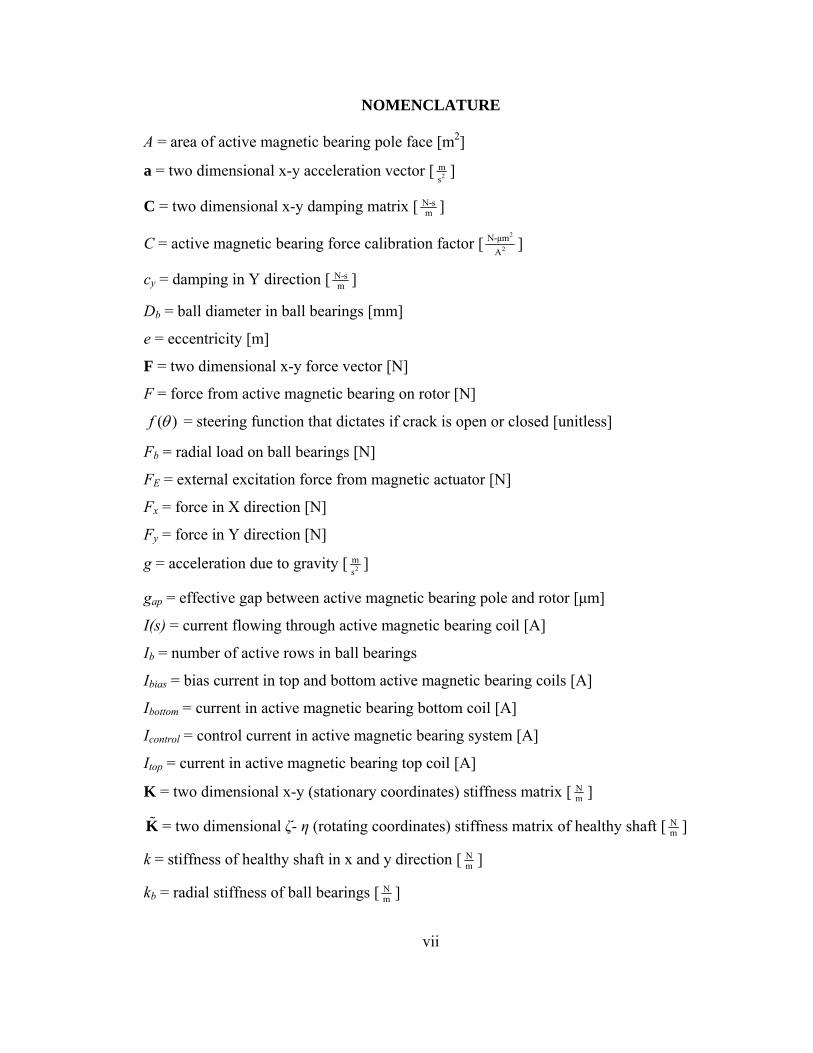
NOMENCLATURE
A = area of active magnetic bearing pole face [m2]
a = two dimensional x-y acceleration vector [ 2ms
]
C = two dimensional x-y damping matrix [ N-sm ]
C = active magnetic bearing force calibration factor [2
2N-μm
A]
cy = damping in Y direction [ N-sm ]
Db = ball diameter in ball bearings [mm]
e = eccentricity [m]
F = two dimensional x-y force vector [N]
F = force from active magnetic bearing on rotor [N]
( )f θ = steering function that dictates if crack is open or closed [unitless]
Fb = radial load on ball bearings [N]
FE = external excitation force from magnetic actuator [N]
Fx = force in X direction [N]
Fy = force in Y direction [N]
g = acceleration due to gravity [ 2ms
]
gap = effective gap between active magnetic bearing pole and rotor [μm]
I(s) = current flowing through active magnetic bearing coil [A]
Ib = number of active rows in ball bearings
Ibias = bias current in top and bottom active magnetic bearing coils [A]
Ibottom = current in active magnetic bearing bottom coil [A]
Icontrol = control current in active magnetic bearing system [A]
Itop = current in active magnetic bearing top coil [A]
K = two dimensional x-y (stationary coordinates) stiffness matrix [ Nm ]
K = two dimensional ζ- η (rotating coordinates) stiffness matrix of healthy shaft [ Nm ]
k = stiffness of healthy shaft in x and y direction [ Nm ]
kb = radial stiffness of ball bearings [ ] Nm
vii
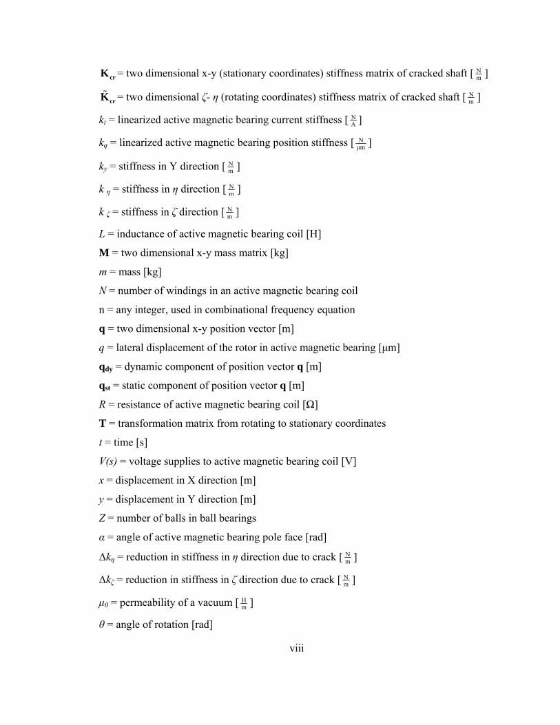
crK = two dimensional x-y (stationary coordinates) stiffness matrix of cracked shaft [ Nm ]
crK = two dimensional ζ- η (rotating coordinates) stiffness matrix of cracked shaft [ Nm ]
ki = linearized active magnetic bearing current stiffness [ NA ]
kq = linearized active magnetic bearing position stiffness [ Nμm ]
k = stiffness in Y direction [yNm ]
k η = stiffness in η direction [ Nm ]
k ζ = stiffness in ζ direction [ Nm ]
windings in an active magnetic bearing coil
magnetic bearing [μm]
]
ry coordinates
e supplies to active magnetic bearing coil [V]
pole face [rad]
k
L = inductance of active magnetic bearing coil [H]
M = two dimensional x-y mass matrix [kg]
m = mass [kg]
N = number of
n = any integer, used in combinational frequency equation
q = two dimensional x-y position vector [m]
q = lateral displacement of the rotor in active
qdy = dynamic component of position vector q [m]
qst = static component of position vector q [m]
R = resistance of active magnetic bearing coil [Ω
T = transformation matrix from rotating to stationa
t = time [s]
V(s) = voltag
x = displacement in X direction [m]
y = displacement in Y direction [m]
Z = number of balls in ball bearings
α = angle of active magnetic bearing
Δkη = reduction in stiffness in η direction due to crac [ Nm ]
Δkζ = reduction in stiffness in ζ direction due to crack [ ] Nm
μ0 = permeability of a vacuum [ Hm ]
θ = angle of rotation [rad]
viii

ix
arings [degrees]
ection [rad]
θb = contact angle in ball be
ψ = angle between whirl vector and crack dir
Ω = combinational frequency [ rads ]
ω = rotor spin speed [ rads ]
ωi = ith natural freque y ofnc the rotor [ rads ]
x
LIST OF TABLES
Table
I. Combinational frequencies corresponding to the rotor test rig supported on ball
bearings………………………………………………………………………………18
II. Nominal masses and moments of inertia for the rotor components………….………26
III. Controller parameters………………………………………………………….…….31
xi
LIST OF FIGURES
Figure
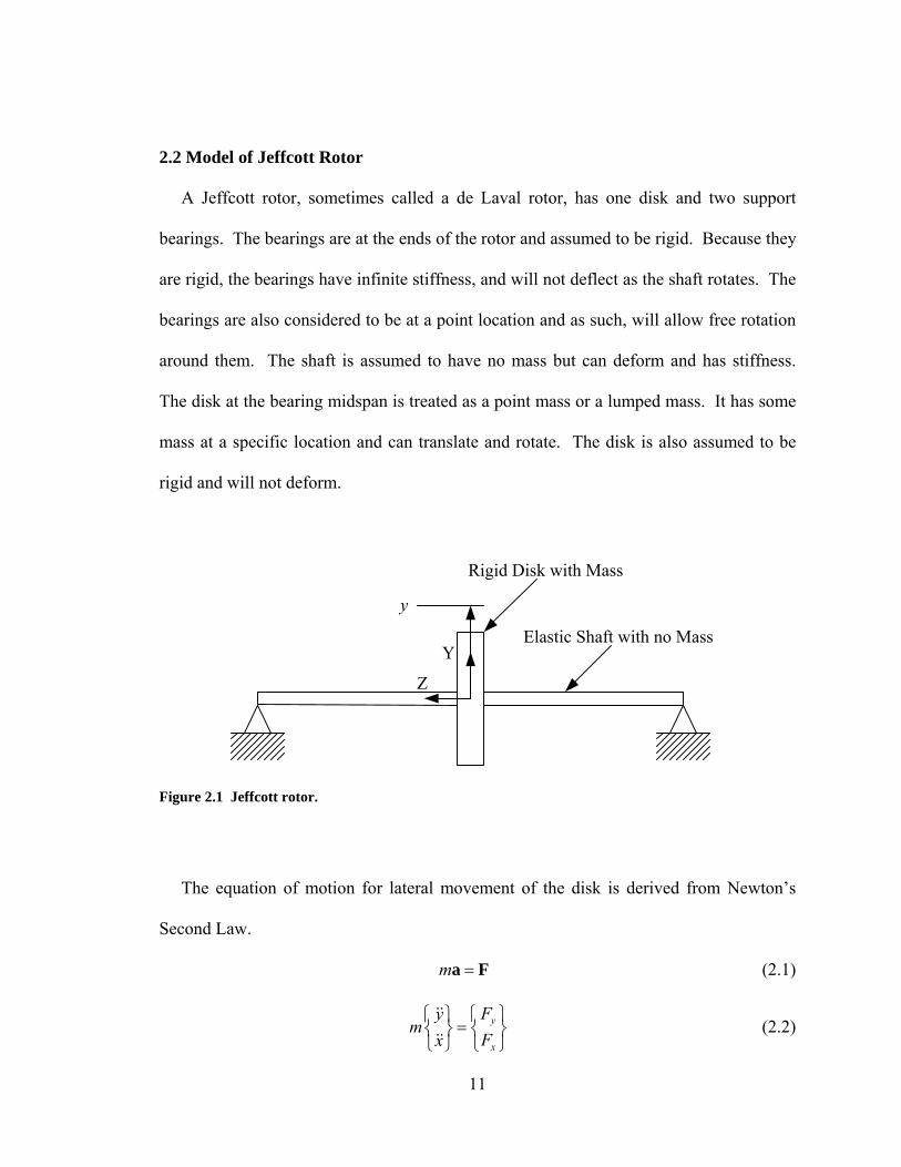
2.1 Jeffcott rotor…………………………………………………………………………11
2.2 Shaft cross section at crack plane near disk showing rotating coordinate
system………………………………………………………………………….…….13
2.3 Gasch and Mayes-Davies transverse crack stiffness reduction steering functions….14
2.4 Cross section of shaft at transverse crack for various rotation angles………………15
2.5 Simulated Jeffcott rotor frequency spectrum of healthy shaft and 25% cracked shaft
rotating at 27 Hz with no force injection………………………………………….…20
2.6 Simulated Jeffcott rotor frequency spectrum of healthy shaft and 25% cracked shaft
rotating at 27 Hz with 10 N force injection at 18 Hz………………………………...20
2.7 Simulated Jeffcott rotor frequency spectrum of healthy shaft and 25% cracked shaft
rotating at 27 Hz with 10 N force injection at 45 Hz……………………………...…21
2.8 Simulated Jeffcott rotor frequency spectrum of healthy shaft and 25% cracked shaft
rotating at 27 Hz with 10 N force injection at 72 Hz……………………………...…21
2.9 Simulated Jeffcott rotor frequency spectrum of healthy shaft and 40% cracked shaft
rotating at 27 Hz with no force injection…………………………………….………22
2.10 Simulated Jeffcott rotor frequency spectrum of healthy shaft and 40% cracked shaft
rotating at 27 Hz with 10 N force injection at 18 Hz………………………..….……22
2.11 Simulated Jeffcott rotor frequency spectrum of healthy shaft and 40% cracked shaft
rotating at 27 Hz with 10 N force injection at 45 Hz……………………………...…23
2.12 Simulated Jeffcott rotor frequency spectrum of healthy shaft and 40% cracked shaft
rotating at 27 Hz with 10 N force injection at 72 Hz…………………………...……23
3.1(a) Crack detection test rig mounted on ball bearings with large disk…………….…26
3.1(b) Major dimensions in inches of the rotor assembly shown with conical magnetic
bearing rotors, exciter’s rotor and unbalance disk. …………………………………26
3.2 Control scheme for one-axis control……………………………………...…………28
3.3 Feedback control loop for one axis active magnetic bearing system with linearized
actuator model………………………………………………………………..………29
xii
3.4 Feedback control loop for 5 axis PID AMB system showing MB340g4-ERX
controller………………………………………………………………..……………30
3.5 Bode plot of the PID controller used for magnetic bearing active control……….…31
3.6 XLRotor finite element model of rotor supported on ball bearings showing
dimensions……………………………………………………………………...……33
3.7 Campbell diagram for rotor on ball bearings…………………………..……………33
3.8 Natural frequencies and mode shapes of the rotor supported on ball bearings…..…34
3.9 Static deflection of the shaft is predicted to be 0.19 mm……………………………35
3.10 Undamped critical speed map showing critical speed as a function of bearing
stiffness………………………………………………………………………………36
3.11 XLRotor finite element model of rotor supported on AMB’s showing
dimensions……………………………………………………………………..…….37
3.12 Campbell diagram for rotor on AMB’s……………………………………………38
3.13 Natural frequencies and mode shapes of the rotor supported on AMB’s………….39
3.14 Force balance between magnetic bearing and shaft reaction force to tune magnetic
bearing calibration factor…………………………………………………….………42
3.15 Dynamic capacity chart for AMB’s showing slew rate……………………………43
4.1 Bottom of a wire EDM cut in a steel 0.625 in. diameter shaft………………...……45
4.2 Bode Plot of undamaged shaft on ball bearings rotating at 600 RPM. Input at
magnetic bearing actuator and output at actuator sensor. Data collected using
MBScope Analyzer tool………………………………………………………..……47
4.3 Close up of first resonance peek of Figure 4.2. Transfer function of damaged shaft
also included for comparison………………………………………………...………47
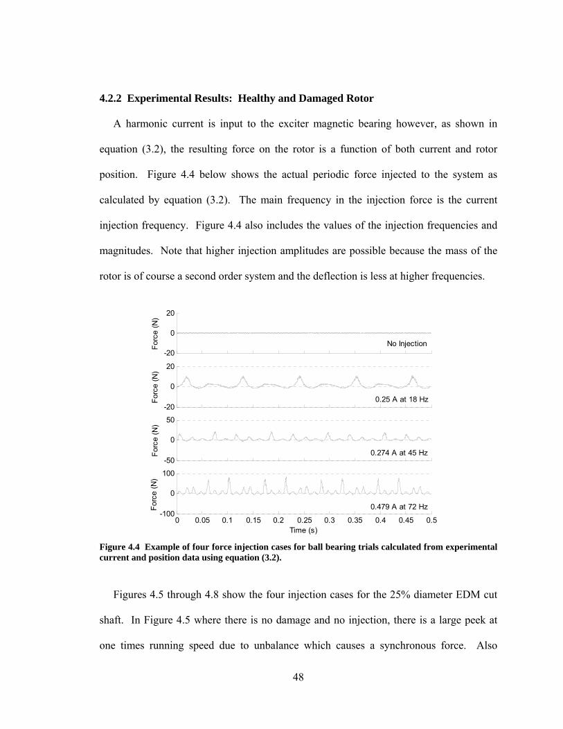
4.4 Example of four force injection cases for ball bearing trials calculated from
experimental current and position data using equation (3.2)…………………..……48
4.5 Frequency spectrum of healthy shaft and 25% EDM (not filled) cut shaft rotating at
27 Hz on ball bearings with no force injection………………………………………50
4.6 Frequency spectrum of healthy shaft and 25% EDM (not filled) cut shaft rotating at
27 Hz on ball bearings with force injection of 0.209 A at 18 Hz……………………50
xiii
4.7 Frequency spectrum of healthy shaft and 25% EDM (not filled) cut shaft rotating at
27 Hz on ball bearings with force injection of 0.221 A at 45 Hz……………………51
4.8 Frequency spectrum of healthy shaft and 25% EDM (not filled) cut shaft rotating at
27 Hz on ball bearings with force injection of 0.297 A at 72 Hz……………………51
4.9 Frequency spectrum of healthy shaft and 40% EDM (not filled) cut shaft rotating at
27 Hz on ball bearings with no force injection………………………………………53
4.10 Frequency spectrum of healthy shaft and 40% EDM (not filled) cut shaft rotating at
27 Hz on ball bearings with force injection of 0.25 A at 18 Hz…………………..…53
4.11 Frequency spectrum of healthy shaft and 40% EDM (not filled) cut shaft rotating at
27 Hz on ball bearings with force injection of 0.274 A at 45 Hz……………………54
4.12 Frequency spectrum of healthy shaft and 40% EDM (not filled) cut shaft rotating at
27 Hz on ball bearings with force injection of 0.368 A at 72 Hz……………………54
4.13 Frequency spectrum of healthy shaft and 25% EDM (filled) cut shaft rotating at 27
Hz on ball bearings with no force injection……………………………………….…56
4.14 Frequency spectrum of healthy shaft and 25% EDM (filled) cut shaft rotating at 27
Hz on ball bearings with force injection of 0.209 A at 18 Hz………………….……56
4.15 Frequency spectrum of healthy shaft and 25% EDM (filled) cut shaft rotating at 27
Hz on ball bearings with force injection of 0.221 A at 45 Hz…………………….…57
4.16 Frequency spectrum of healthy shaft and 25% EDM (filled) cut shaft rotating at 27
Hz on ball bearings with force injection of 0.299 A at 72 Hz…………….…………57
4.17 Frequency spectrum of healthy shaft and 40% EDM (filled) cut shaft rotating at 27
Hz on ball bearings with no force injection…………………………………….……59
4.18 Frequency spectrum of healthy shaft and 40% EDM (filled) cut shaft rotating at 27
Hz on ball bearings with force injection of 0.25 A at 18 Hz…………………...……59
4.19 Frequency spectrum of healthy shaft and 40% EDM (filled) cut shaft rotating at 27
Hz on ball bearings with force injection of 0.274 A at 45 Hz………………….……60
4.20 Frequency spectrum of healthy shaft and 40% EDM (filled) cut shaft rotating at 27
Hz on ball bearings with force injection of 0.368 A at 72 Hz…………………….…60
4.21 Comparison of difference from control test for simulation and experimental results
for 40% cut shaft and no injection (See Figures 2.9, 4.9 and 4.17)…………………61
xiv
4.22 Comparison of difference from control test for simulation and experimental results
for 40% cut shaft and 18 Hz injection (See Figures 2.10, 4.10 and 4.18)………...…61
4.23 Comparison of difference from control test for simulation and experimental results
for 40% cut shaft and 45 Hz injection (See Figures 2.11, 4.11 and 4.19)……….…..62
4.24 Comparison of difference from control test for simulation and experimental results
for 40% cut shaft and 72 Hz injection (See Figures 2.12, 4.12 and 4.20)………...…62
4.25 Simulink model used to test manufacturer provided PID control values……….…64
4.26 Model of controller and AMB used in Simulink model shown in Figure 4.21……64
4.27 Impulse response of simulated magnetically levitated rotor………………………65
4.28 Impulse response of simulated magnetically levitated rotor including force due to
unbalance……………………………………………………………………….……65
4.29 Alternate model of controller and AMB used in Simulink model shown in Figure
4.21………………………………………………………………………………...…66
4.30 Bode Plot of undamaged shaft on magnetic bearings. Input at magnetic bearing
actuator and output at actuator sensor. Data collected using MBScope Analyzer
tool………………………………………………………………………..………….67
4.31 Close up of first resonance peek of Figure 4.30. Transfer function of damaged shaft
also included for comparison……………………………………………………...…67
4.32 Example of four force injection cases for magnetic bearing trials calculated from
experimental current and position data using equation (3.2)…………………...……68
4.33 Frequency spectrum of healthy shaft and 40% EDM (not filled) cut shaft rotating at
22.5 Hz on active magnetic bearings with no force injection………………..………70
4.34 Frequency spectrum of healthy shaft and 40% EDM (not filled) cut shaft rotating at
22.5 Hz on active magnetic bearings with force injection of 0.097 A at 15 Hz…..…70
4.35 Frequency spectrum of healthy shaft and 40% EDM (not filled) cut shaft rotating at
22.5 Hz on active magnetic bearings with force injection of 0.097 A at 37.5 Hz…..71
4.36 Frequency spectrum of healthy shaft and 40% EDM (not filled) cut shaft rotating at
22.5 Hz on active magnetic bearings with force injection of 0.097 A at 60 Hz……..71
CHAPTER I
INTRODUCTION
1.1 Background and Motivation
Simply put, work is force times distance. And, power is the time rate change of work.
Another way of saying this is power is force times speed. Rotating machinery offer a
way to achieve high speeds in compact, efficient, able to be harnessed ways. It is
because of this that the modern world is built upon rotating machinery, be it a turbine
used for power generation, a mill used for manufacturing, or a jet engine used for travel.
A failure in a rotating machine can potentially be dangerous to people in the vicinity and
costly to repair. The time the machine is stopped for repair can be more costly than the
actual machine itself. Rieger et al [1990] reported on the costs associated with rotating
machinery failure.
1
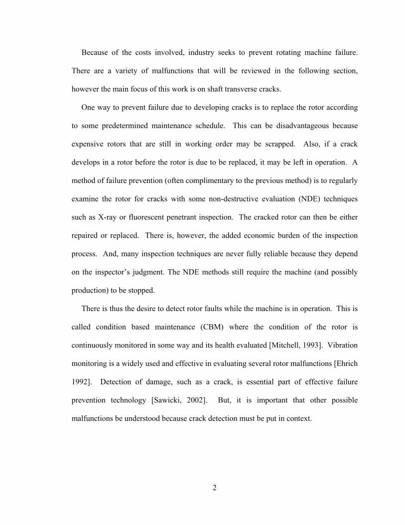
Because of the costs involved, industry seeks to prevent rotating machine failure.
There are a variety of malfunctions that will be reviewed in the following section,
however the main focus of this work is on shaft transverse cracks.
One way to prevent failure due to developing cracks is to replace the rotor according
to some predetermined maintenance schedule. This can be disadvantageous because
expensive rotors that are still in working order may be scrapped. Also, if a crack
develops in a rotor before the rotor is due to be replaced, it may be left in operation. A
method of failure prevention (often complimentary to the previous method) is to regularly
examine the rotor for cracks with some non-destructive evaluation (NDE) techniques
such as X-ray or fluorescent penetrant inspection. The cracked rotor can then be either
repaired or replaced. There is, however, the added economic burden of the inspection
process. And, many inspection techniques are never fully reliable because they depend
on the inspector’s judgment. The NDE methods still require the machine (and possibly
production) to be stopped.
There is thus the desire to detect rotor faults while the machine is in operation. This is
called condition based maintenance (CBM) where the condition of the rotor is
continuously monitored in some way and its health evaluated [Mitchell, 1993]. Vibration
monitoring is a widely used and effective in evaluating several rotor malfunctions [Ehrich
1992]. Detection of damage, such as a crack, is essential part of effective failure
prevention technology [Sawicki, 2002]. But, it is important that other possible
malfunctions be understood because crack detection must be put in context.
2
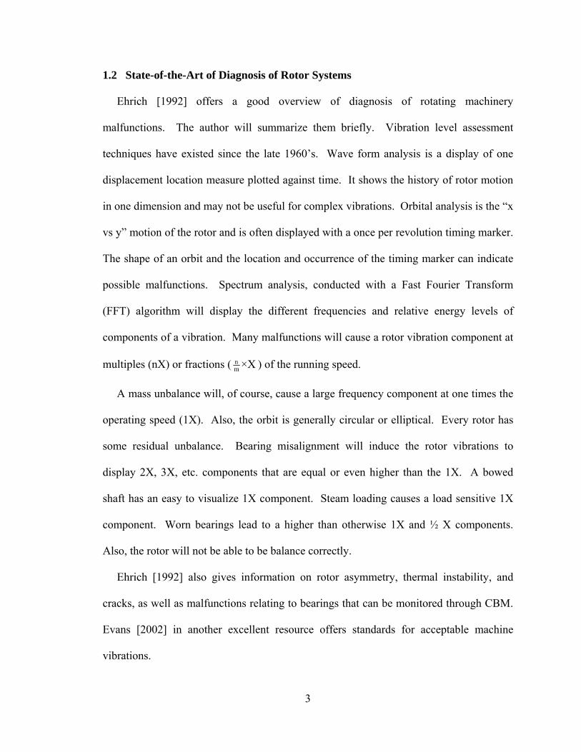
1.2 State-of-the-Art of Diagnosis of Rotor Systems
Ehrich [1992] offers a good overview of diagnosis of rotating machinery
malfunctions. The author will summarize them briefly. Vibration level assessment
techniques have existed since the late 1960’s. Wave form analysis is a display of one
displacement location measure plotted against time. It shows the history of rotor motion
in one dimension and may not be useful for complex vibrations. Orbital analysis is the “x
vs y” motion of the rotor and is often displayed with a once per revolution timing marker.
The shape of an orbit and the location and occurrence of the timing marker can indicate
possible malfunctions. Spectrum analysis, conducted with a Fast Fourier Transform
(FFT) algorithm will display the different frequencies and relative energy levels of
components of a vibration. Many malfunctions will cause a rotor vibration component at
multiples (nX) or fractions ( nm ×X ) of the running speed.
A mass unbalance will, of course, cause a large frequency component at one times the
operating speed (1X). Also, the orbit is generally circular or elliptical. Every rotor has
some residual unbalance. Bearing misalignment will induce the rotor vibrations to
display 2X, 3X, etc. components that are equal or even higher than the 1X. A bowed
shaft has an easy to visualize 1X component. Steam loading causes a load sensitive 1X
component. Worn bearings lead to a higher than otherwise 1X and ½ X components.
Also, the rotor will not be able to be balance correctly.
Ehrich [1992] also gives information on rotor asymmetry, thermal instability, and
cracks, as well as malfunctions relating to bearings that can be monitored through CBM.
Evans [2002] in another excellent resource offers standards for acceptable machine
vibrations.
3
Many machine monitoring methods incorporate system modeling [Sawicki 2001].
Comparing the model to the state of the rotor system can indicate if the rotor is healthy or
faulty. During run up and cost down, the rotor passes through a range of speeds. With
this information, and the vibration magnitudes at each speed, a bode plot can be drawn
[Bently 1995] and [Muszynska 1995]. Obviously, this is disadvantageous because it still
required the machine to be stopped. However in systems that start and stop often
anyway, it can be more useful. Online perturbation for gathering similar data is also
explored.
One rotor malfunction that has recently received much study, both experimental and
through simulation is rubbing. Adams [2001] used a Jeffcott rotor simulation to show the
usefulness of bifurcation diagrams and Poincare map in identifying impact-rubbing
behavior. Spectra power analysis is also used to interpret the highly nonlinear dynamics.
Sawicki et al [2003] experimentally investigated the sub-harmonics and amplitude
discontinuities of rotor stator rubbing. Also, Sawicki [1999] analyzed experimentally
identify sub harmonics caused by rubbing using FFT and Al-Khatib [1997] was able to
show system parameter changes that could not be detected with FFT could be detected
using bifurcation diagrams and Poincare maps. Al-Khatib showed the potential of chaos
signal processing in this area.
One interesting aspect of rotor rubbing is the thermal consequences and how
vibrations are affected. Taylor [1924] studied shaft rubbing above and below the critical
speed and after Taylor’s results, Newkirk [1926] pointed out that rubbing below the first
critical speed brings with it vibrations with amplitude increasing with time. This is due to
uneven heating of the shaft and subsequent thermal expansion causing warping. More
4
recent studies in this area include [Dimaroganas 1973], [Dimaroganas 1983], and
[Muszynska 1993]. Kellenberger [1980] studied this effect in turbogenerators in relation
to seal rings.
An example of an industry greatly concerned with all types of rotating machinery
malfunctions and how to detect them online is the jet engine industry. Two recent studies
in this area are [Gyekenyesi 2002] and [Baaklini 2002]. The application of health
diagnosis through vibration monitoring is examined.
Dimarogonas [1996] conducted a review of the vibration of cracked structures and
Doebling et al [1996] conducted an extensive survey of the crack detection field
including works using external force perturbation. The survey does not include rotating
machinery, but it is useful for further detail on the topic.
The most basic form of crack detection is by observing the vibration for a 2X
frequency component. Dimentberg [1961] showed that the total motion of an asymmetric
shaft center is the sum of a vector that turns with the angular velocity and a vector that
turns with twice the angular velocity. The result is a spiral like orbit that is determined
by the relative lengths of the two vectors. The reason for this phenomenon is the shaft
switches between a strong axis and weak axis twice per revolution. When the weak axis
is resisting gravity the shaft sits lower than when the strong axis does. This oscillation
added to the dynamic orbit of the shaft causes the 2X component. A transverse crack
makes a shaft have asymmetric stiffness.
Unlike a simple asymmetric shaft, a shaft with a transverse crack may exhibit so
called breathing. That is the crack opens and closes with the rotation of the shaft. The
crack will be open when it is directed downward because the shaft bends downward with
5
its own weight. The crack will likewise be closed when it is directed upward because the
shaft is bowed away from it. This is of course only the case when the weight of the shaft
is greater than the dynamic force due to rotation. This is called weight dominance. If
dynamic forces are greater than the weight, the crack will either remain closed or open,
depending on the crack’s phase with relation to high spot. Weight dominance will be the
assumption for the analysis in this work.
For a transverse crack in a shaft under weight dominance, Gasch [1976] proposed a
hinge like model for the opening and closing of the crack and subsequent time varying
stiffness. In his work, the crack opens and closed abruptly, changing from maximum to
minimum stiffness instantly and the motion of the rotor was analyzed. A modified crack
model was put forth by Mayes [1976] where the crack opens and closes with a cosine
function. Simulations using fracture mechanics have shown that the two models’
behavior is nearly identical [Jun 1992]. Gasch [1993] conducted a survey of the topic
which should be consulted for further detail. Another survey that is a good resource is
[Wauer 1990].
All of the above techniques for health monitoring are passive. That is, they do not
affect the rotor and only observe its motion. In order to widen the range of situations
where online health monitoring is affective, active methods were explored. Active online
monitoring is where the rotor is affected in some way and the response in observed. By
comparing the response to the expected response, the state of the system can be
monitored. Rotating systems present certain difficulties in active monitoring because of
their motion. It will be seen that active magnetic bearings (AMB), either as an additional
6
actuator to a conventional bearing system or through a superimposed signal injection to a
full AMB system is a useful tool to active condition monitoring to rotating machinery.
Morton [1975] was one of the first who identified dynamic properties of a full
operating turbomachine by means of a broadband excitation technique. The rotating shaft
was preloaded with a static force via an additional foil bearing. The excitation force was
created by a sudden release of the preload due to the use of a breaking link, while the
applied forces were measured with strain gauges. The method was used for the
identification of rotordynamic coefficients of oil film bearings. Nordmann [1984] and
Tonnesen [1988] excited a rotating Jeffcott rotor supported on oil film bearings by a
hammer. The impact force and displacement signals were used for identification of the
modal parameters of the rotating system. One of the disadvantages of the broadband
excitation in general is the distribution of the energy over a certain frequency range,
which may cause a poor signal to noise ratio. Iwatsubo et al. [1992] used external
excitation technique to analyze the response of the cracked shaft. He showed the presence
of combination harmonics due to interaction between impact force and rotation of shaft
as the crack indicators.
Nordmann [2004] showed experimentally that the transfer function of a centrifugal
pump levitated in AMB’s could be measured and used to diagnose faults. Bash [2005]
used AMB actuator to perform a sine sweep on a test rotor and measure the change in
natural frequency due to a transverse crack. Kasarda et al [2005] showed experimentally
that AMB could be used to accurately excite natural frequencies of a test rig with a
variety of input types such as sine sweep and random noise. Also, the usefulness of these
measurements was demonstrated using simulations. Quinn et al [2005] showed
7
experimentally that timed force injections from an AMB can be used to identify the time
varying stiffness of a rotor with a transverse crack.
Penny et al [2006] and Mani et al [2006] showed with numerical simulations that the
combinational frequencies present in a cracked rotating system can be excited by a
harmonic force input from a magnetic bearing (MB). Sawicki et al [2008] confirmed the
simulations with experimental results. Also, the sub harmonics in such a system were
experimentally found using a sine sweep from AMB actuator [Ishida 2006].
1.3 Scope of Work
The aim of this thesis is to investigate a novel structural health monitoring approach
for the detection of damage in a form of transverse crack in rotating shafts, which utilizes
an active magnetic bearing (AMB) as an actuator for applying multiple types of force
inputs on to a rotating structure for analysis of resulting outputs. To that end, the scope
of this work includes discussing and demonstrating the approach. Discussion of the
approach will include the modeling of a simple Jeffcott rotor, evaluation how a transverse
crack and force injection will affect the model, and making predictions for the rotor’s
motion using numerical integration. Demonstrating the approach will enforce the
prediction with experimental results. The experimental test rig will be described and the
dynamics will be identified using FEA and a sine sweep analysis. Then actual position
data will be taken for a “healthy” i.e., undamaged shaft running on ball bearings and
compared to that for a damaged shaft under the same conditions. To ad breadth to the
demonstration the same comparison will be made for a rotor levitated on active magnetic
bearings.
8
In Chapter 2 the modeling of the Jeffcott rotor will be provided and used to make
prediction for the difference in motion of a cracked and un-cracked Jeffcott rotor when it
is harmonically excited. Chapter 3 will describe the test rig used to perform the
experiment in detail, including rotor configuration, data acquisition, magnetic bearing
modeling, and force estimation. The results of the experiment will be presented and
discussed in Chapter 4. Chapter 4 will include a section for the rotor on traditional ball
bearing supports and a section for the rotor levitated magnetically. Conclusions and
recommendations will be in Chapter 5.
9
CHAPTER II
THE CRACKED JEFFCOTT ROTOR
2.1 Introduction
The crack detection approach investigated in this work can be fully demonstrated by
experiment alone. However, to gain a deeper understanding of the method and when it is
applicable, equations of motion for a rotating, externally excited rotor will be derived, for
the healthy case and cracked case, and the solutions will be found numerically. A
Jeffcott rotor model will be used in the modeling for simplicity. The solution will serve
as a rough prediction for the experimental results in terms of the general form but not in
terms of actual values because the Jeffcott rotor is an idealized model which does not
resemble the actual test rig. Actual physical parameter values of the test rig will be used
to generate values for the Jeffcott rotor model with the intention of making the solution
on the similar order as the actual experimental results.
10
2.2 Model of Jeffcott Rotor
A Jeffcott rotor, sometimes called a de Laval rotor, has one disk and two support
bearings. The bearings are at the ends of the rotor and assumed to be rigid. Because they
are rigid, the bearings have infinite stiffness, and will not deflect as the shaft rotates. The
bearings are also considered to be at a point location and as such, will allow free rotation
around them. The shaft is assumed to have no mass but can deform and has stiffness.
The disk at the bearing midspan is treated as a point mass or a lumped mass. It has some
mass at a specific location and can translate and rotate. The disk is also assumed to be
rigid and will not deform.
y
Z
Y
Rigid Disk with Mass
Elastic Shaft with no Mass
Figure 2.1 Jeffcott rotor.
The equation of motion for lateral movement of the disk is derived from Newton’s
Second Law.
m =a F (2.1)
y
x
Fym
Fx⎧ ⎫⎧ ⎫
=⎨ ⎬ ⎨ ⎬⎩ ⎭ ⎩ ⎭
(2.2)
11
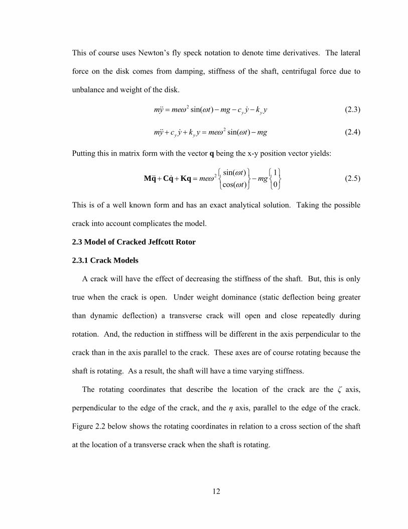
This of course uses Newton’s fly speck notation to denote time derivatives. The lateral
force on the disk comes from damping, stiffness of the shaft, centrifugal force due to
unbalance and weight of the disk.
(2.3) 2 sin( ) y ymy me t mg c y k yω ω= − − −
2 sin( )y ymy c y k y me t mgω ω+ + = − (2.4)
Putting this in matrix form with the vector q being the x-y position vector yields:
2 sin( ) 1cos( ) 0
tme mg
tω
ωω
⎧ ⎫ ⎧+ + = −
⎫⎨ ⎬ ⎨⎩ ⎭ ⎩
Mq Cq Kq ⎬⎭
(2.5)
This is of a well known form and has an exact analytical solution. Taking the possible
crack into account complicates the model.
2.3 Model of Cracked Jeffcott Rotor
2.3.1 Crack Models
A crack will have the effect of decreasing the stiffness of the shaft. But, this is only
true when the crack is open. Under weight dominance (static deflection being greater
than dynamic deflection) a transverse crack will open and close repeatedly during
rotation. And, the reduction in stiffness will be different in the axis perpendicular to the
crack than in the axis parallel to the crack. These axes are of course rotating because the
shaft is rotating. As a result, the shaft will have a time varying stiffness.
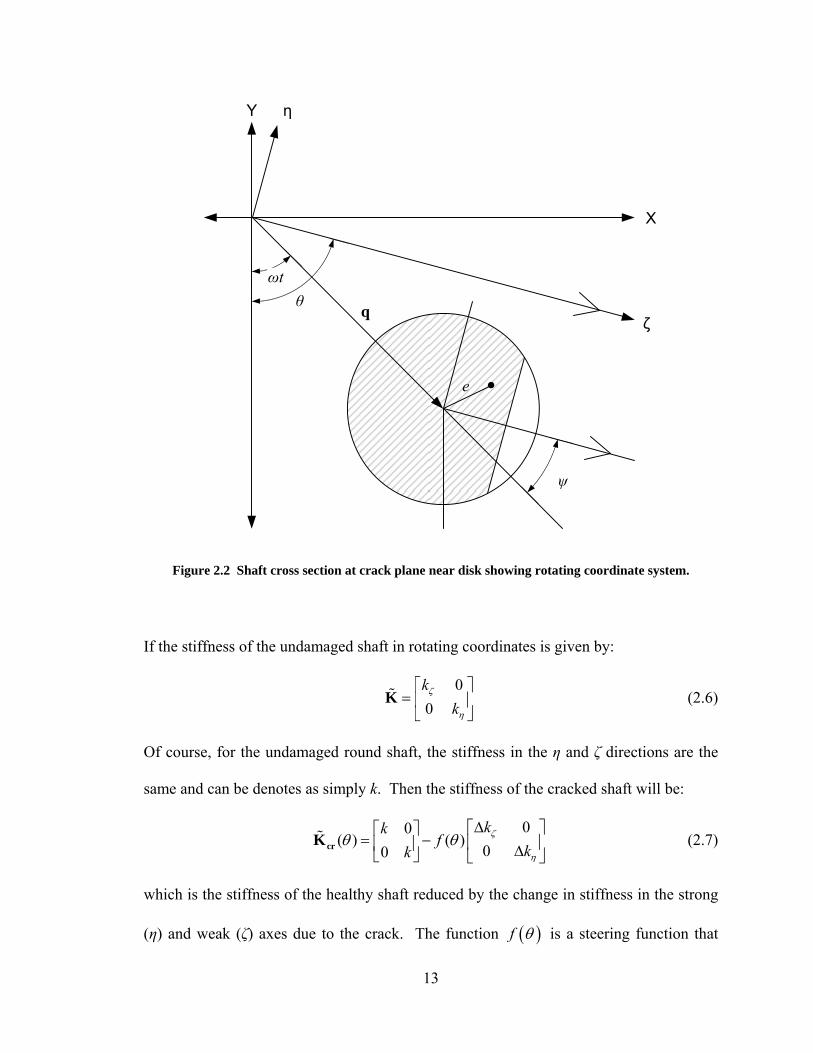
The rotating coordinates that describe the location of the crack are the ζ axis,
perpendicular to the edge of the crack, and the η axis, parallel to the edge of the crack.
Figure 2.2 below shows the rotating coordinates in relation to a cross section of the shaft
at the location of a transverse crack when the shaft is rotating.
12
X
Y
ζ
η
e
θ
ψ
ωt
q
Figure 2.2 Shaft cross section at crack plane near disk showing rotating coordinate system.
If the stiffness of the undamaged shaft in rotating coordinates is given by:
00k
kζ
η
⎡ ⎤= ⎢ ⎥⎣ ⎦
K (2.6)
Of course, for the undamaged round shaft, the stiffness in the η and ζ directions are the
same and can be denotes as simply k. Then the stiffness of the cracked shaft will be:
00( ) ( )
00kk
fkk
ζ
η
θ θΔ⎡ ⎤⎡ ⎤
= − ⎢ ⎥⎢ ⎥ Δ⎣ ⎦ ⎣ ⎦crK (2.7)
which is the stiffness of the healthy shaft reduced by the change in stiffness in the strong
(η) and weak (ζ) axes due to the crack. The function ( )f θ is a steering function that
13
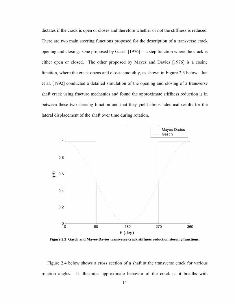
dictates if the crack is open or closes and therefore whether or not the stiffness is reduced.
There are two main steering functions proposed for the description of a transverse crack
opening and closing. One proposed by Gasch [1976] is a step function where the crack is
either open or closed. The other proposed by Mayes and Davies [1976] is a cosine
function, where the crack opens and closes smoothly, as shown in Figure 2.3 below. Jun
et al. [1992] conducted a detailed simulation of the opening and closing of a transverse
shaft crack using fracture mechanics and found the approximate stiffness reduction is in
between these two steering function and that they yield almost identical results for the
lateral displacement of the shaft over time during rotation.
0 90 180 270 3600
0.2
0.4
0.6
0.8
1
f(θ )
θ (deg)
Mayes-DaviesGasch
Figure 2.3 Gasch and Mayes-Davies transverse crack stiffness reduction steering functions.
Figure 2.4 below shows a cross section of a shaft at the transverse crack for various
rotation angles. It illustrates approximate behavior of the crack as it breaths with
14
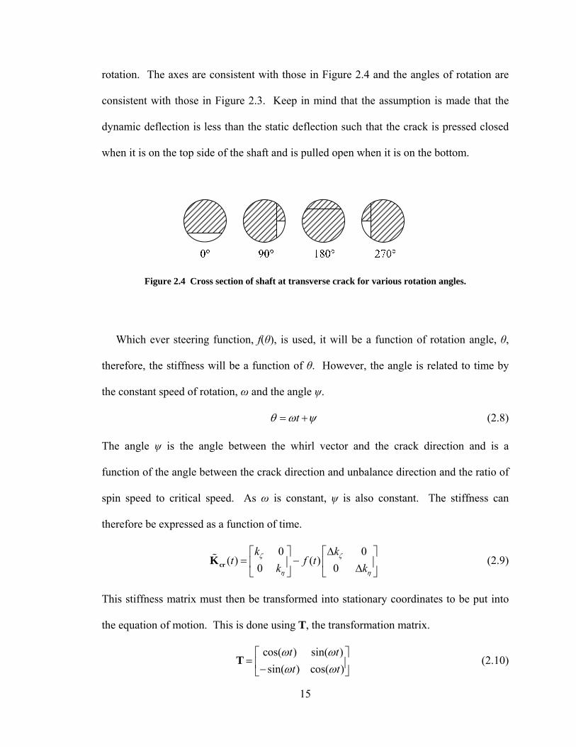
rotation. The axes are consistent with those in Figure 2.4 and the angles of rotation are
consistent with those in Figure 2.3. Keep in mind that the assumption is made that the
dynamic deflection is less than the static deflection such that the crack is pressed closed
when it is on the top side of the shaft and is pulled open when it is on the bottom.
Figure 2.4 Cross section of shaft at transverse crack for various rotation angles.
Which ever steering function, f(θ), is used, it will be a function of rotation angle, θ,
therefore, e by
e constant speed of rotation, ω and the angle ψ.
the stiffness will be a function of θ. However, the angle is related to tim
th
tθ ω ψ= + (2.8)
The angle ψ is the angle between the whirl vector and the crack direction and is a
function of the angle between the crack direction and unbalance direction and the ratio of
spin speed to critical speed. As ω is constant, ψ is also constant. The stiffness can
therefore be expressed as a function of time.
0 00 0k k
k kζ ζ( ) ( )t f t
η η
Δ⎡ ⎤ ⎡ ⎤= −⎢ ⎥ ⎢ ⎥Δ⎣ ⎦ ⎣ ⎦
cr
This stiffness matrix must then be transform
K (2.9)
ed into stationary coordinates to be put into
the equation of motion. This is done using T, the transformation matrix.
cos( ) sin( )sin( ) cos( )
t tt t
ω ωω ω
⎡ ⎤= ⎢ ⎥−⎣ ⎦
T (2.10)
15
( ) ( )t tTcr crK = T K T (2.11)
00 kk ⎛ ⎞Δ( ) ( )
00t f t
kkζ⎡ ⎤⎡ ⎤
η
= − ⎜ ⎟⎢ ⎥⎢ ⎥ ⎜ ⎟Δ⎣ ⎦ ⎣ ⎦ ⎠⎝
TcrK T T (2.12)
2.3.2 Equation of Motion of a Cracked Jeffcott R
Substituting the stiffness matrix for the cracked Jeffcott rotor in stationary coordinates
into the equation of motion for the healthy Jeffcott rotor gives the equation of motion for
e cracked Jeffcott rotor. Note that Kcr is a function of time.
otor
th
2 sin( ) 1cos( ) 0
tt
ωω
( )t me mgω⎧ ⎫ ⎧ ⎫
+ + = −⎨ ⎬ ⎨crMq Cq K q ⎬ (2.13)
he position vector q can be separated into its static and dynamic components, qst and
qdy respectively.
⎩ ⎭ ⎩ ⎭
T
= +st dyq q q (2.14)
ubstituting equation (2.14) into equation (2.13) gives:
g
S
( ) 2 sin( ) 1( )
cos( ) 0t
t me mt
ωωω⎧ ⎫ ⎧
+ + + = −⎫
⎨ ⎬ ⎨⎩ ⎭ ⎩
dy dy cr st dyMq Cq K q q ⎬⎭
(2.15)
As the shaft rotates and the crack opens and close
cause the change in stiffness due
to a crack is usually small and the resulting change in static equilibrium is small. With
this simplification, the static displacement is constant and effectively equal to the weight
s, the stiffness changes and so the static
displacement will change. This change is neglected be
divided by the stiffness of the healthy shaft. The static displacement multiplied by the
stiffness cancels out with weight yielding equation (2.16).
16
2 sin( )( )
cos( )t
t met
ωω
ω⎧ ⎫
+ + = ⎨ ⎬dy dy cr dyMq Cq K q⎩ ⎭
(2.16)
Equation (2.5) is the equation of motion for a Jeffcott rotor. Equation (2.5) is
modified for a transverse crack and the weight dominance assumption to get equation
(2.16). For the active crack detection method, the equation must again be modified to
include an external force.
2 sin( ) sin( )( )
cos( ) 0Et F t
t met
ωω
ωΩ⎧ ⎫ ⎧ ⎫
+ + = +⎨ ⎬ ⎨ ⎬dy dy cr dyMq Cq K q⎩ ⎭ ⎩ ⎭
(2.17)
Here, FE is the magnitude of external excitation and Ω is the frequency of excitation
which will be discussed in the next section.
2.4 Combinational Frequency Excitation
tion frequency at which resonance occurs.
ani et al. (2005) and Quinn et al. (2005) used multiple scales analysis to determine the
frequencies. This is given by the following
There exists in such a system, frequencies that are the combination of the running
speed, natural frequencies, and external injec
M
conditions required for these combinational
equation.
inω ωΩ = − , for n = ±1, ±2, ±3 ... (2.18)
where Ω is the combinational frequency, ω is the rotor spin speed and ωi is the ith natural
equency. Note that because of the particular assumptions made for the Jeffcott rotor,
the system only has one natural freque
atural frequency of the test rig. By selecting an n value, solving for Ω and injecting that
fr
ncy and that it will be tuned to match the first
n
17
frequency into the system, the combinational frequencies corresponding to all other n
values will be induced and can be observed if damage such as a crack is present. In the
Jeffcott rotor simulation, an external force excitation is applied to the disk in the direction
of gravity. It is this force, at such a frequency, that provides external excitation and
excites resonances at the combinational frequencies. Because the Jeffcott rotor model
has the same natural frequency (36 Hz) and running speed (27 Hz) as the experimental
test rig on ball bearings, the combinational frequency values are the same. Some of these
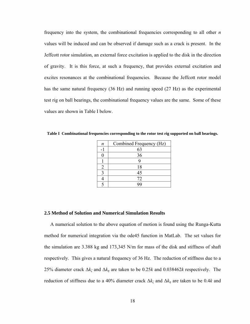
values are shown in Table I below.
Table I Combinational frequencies corresponding to the rotor test rig supported on ball bearings.
n Combined Frequency (Hz) -1 63 0 36 1 9 2 18 3 45 4 72 5 99
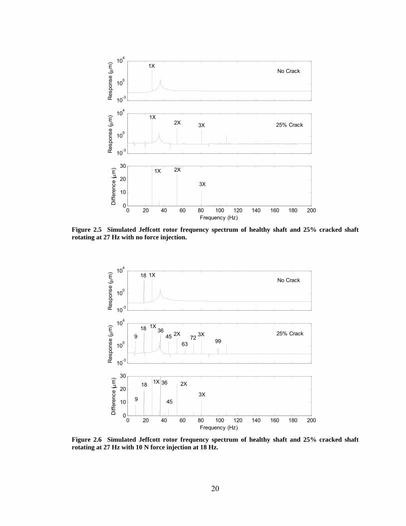
2.5 Method of Solution and merical Simu esults
A numerical solution to th above equation of motion is found using the Runga-Kutta
ethod for numerical integration via the ode45 function in MatLab. The set values for
e simulation are 3.388 kg and 173,345 N/m for mass of the disk and stiffness of shaft
uction of stiffness due to a
Nu lation R
e
m
th
respectively. This gives a natural frequency of 36 Hz. The red
25% diameter crack Δkζ and Δkη are taken to be 0.25k and 0.038462k respectively. The
reduction of stiffness due to a 40% diameter crack Δkζ and Δkη are taken to be 0.4k and
18
0.0678k respectively. Here, Δkζ is assumed and Δkη is found using the axis stiffness
reduction ratio interpolated from Gasch (1993). The rotation is set at 27 Hz. Damping is
taken as 5 N-sm in both x and y directions with no cross coupling. The external excitation
amplitude was set at 10 N. Remember that the values are chosen to be similar to the
actual experimental rig but the rig is not a true Jeffcott rotor so the simulation only makes
a prediction as to the approximate form of the experimental results.
After th position over time is solved for, the Fast Fourier Transform (FFT) is
performed. The time sampling was selected so as to have an integer number of vibrations
and a number of samples equal to a power of two in order to minimize leakage. The first
few seconds are discarded to minimize transient effect however a s
e
mall peak can still be
seen at the natural frequency.
19
10-3
100
104
Res
pons
e ( μ
m)
10-3
100
104R
espo
nse
( μm
)
0 20 40 60 80 100 120 140 160 180 2000
10
20
30
Diff
eren
ce ( μ
m)
Frequency (Hz)
1X No Crack
1X 2X 3X 25% Crack
1X 2X
3X
Figure 2.5 Simulated Jeffcott rotor frequency spectrum of healthy shaft and 25% cracked shaft rotating at 27 Hz with no force injection.
10-3
100
104
Res
pons
e ( μ
m)
10-3
100
104
Res
pons
e ( μ
m)
0 20 40 60 80 100 120 140 160 180 2000
10
20
30
Diff
eren
ce ( μ
m)
Frequency (Hz)
18 1X No Crack
918 1X
36 45 2X
6372 3X
9925% Crack
9
18 1X 36
45
2X
3X
Figure 2.6 Simulated Jeffcott rotor frequency spectrum of healthy shaft and 25% cracked shaft rotating at 27 Hz with 10 N force injection at 18 Hz.
20
10-3
100
104
Res
pons
e ( μ
m)
10-3
100
104R
espo
nse
( μm
)
0 20 40 60 80 100 120 140 160 180 2000
10
20
30
Diff
eren
ce ( μ
m)
Frequency (Hz)
1X 45No Crack
91X
36 45
2X 63 72
3X 99
25% Crack
918
1X 36 2X
3X
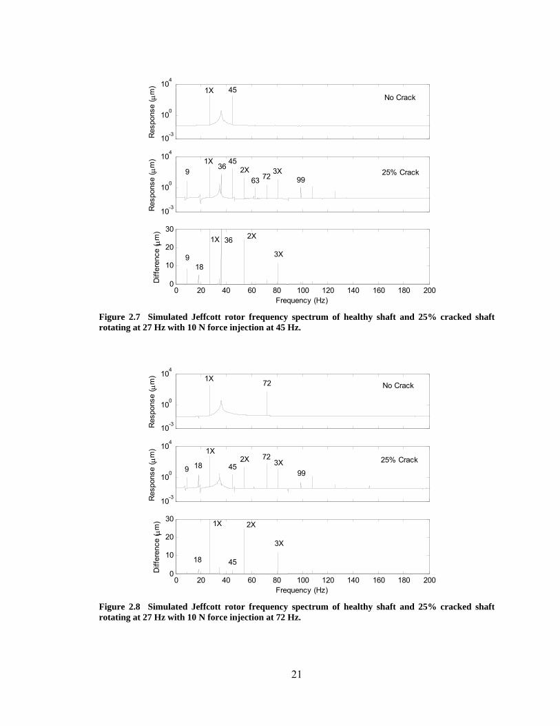
Figure 2.7 Simulated Jeffcott rotor frequency spectrum of healthy shaft and 25% cracked shaft rotating at 27 Hz with 10 N force injection at 45 Hz.
10-3
100
104
Res
pons
e ( μ
m)
10-3
100
104
Res
pons
e ( μ
m)
0 20 40 60 80 100 120 140 160 180 2000
10
20
30
Diff
eren
ce ( μ
m)
Frequency (Hz)
1X 72 No Crack
25% Crack 9 18
1X
452X 72
3X 99
18 45
1X 2X
3X
Figure 2.8 Simulated Jeffcott rotor frequency spectrum of healthy shaft and 25% cracked shaft rotating at 27 Hz with 10 N force injection at 72 Hz.
21
10-3
100
104
Res
pons
e ( μ
m)
10-3
100
104R
espo
nse
( μm
)
0 20 40 60 80 100 120 140 160 180 2000
10
20
30
Diff
eren
ce ( μ
m)
Frequency (Hz)
No Crack
40% Crack
1X 2X 3X
3X 2X 1X
1X
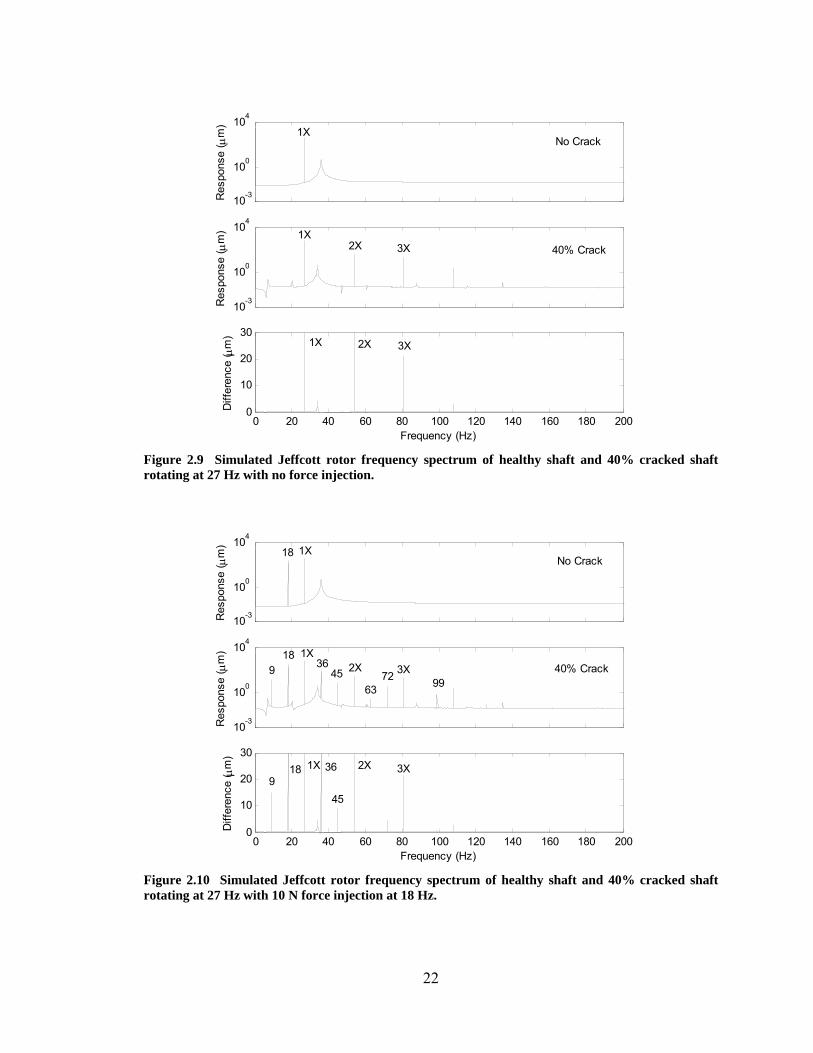
Figure 2.9 Simulated Jeffcott rotor frequency spectrum of healthy shaft and 40% cracked shaft rotating at 27 Hz with no force injection.
10-3
100
104
Res
pons
e ( μ
m)
10-3
100
104
Res
pons
e ( μ
m)
0 20 40 60 80 100 120 140 160 180 2000
10
20
30
Diff
eren
ce ( μ
m)
Frequency (Hz)
No Crack
40% Crack
1X
1X 2X 3X
1X 2X 3X
918
36 45
6372 99
918 36
45
18
Figure 2.10 Simulated Jeffcott rotor frequency spectrum of healthy shaft and 40% cracked shaft rotating at 27 Hz with 10 N force injection at 18 Hz.
22
10-3
100
104
Res
pons
e ( μ
m)
10-3
100
104R
espo
nse
( μm
)
0 20 40 60 80 100 120 140 160 180 2000
10
20
30
Diff
eren
ce ( μ
m)
Frequency (Hz)
40% Crack
No Crack
18
1X 2X
9
3X 36
1X 45
9 18
1X 452X
63 723X
9936
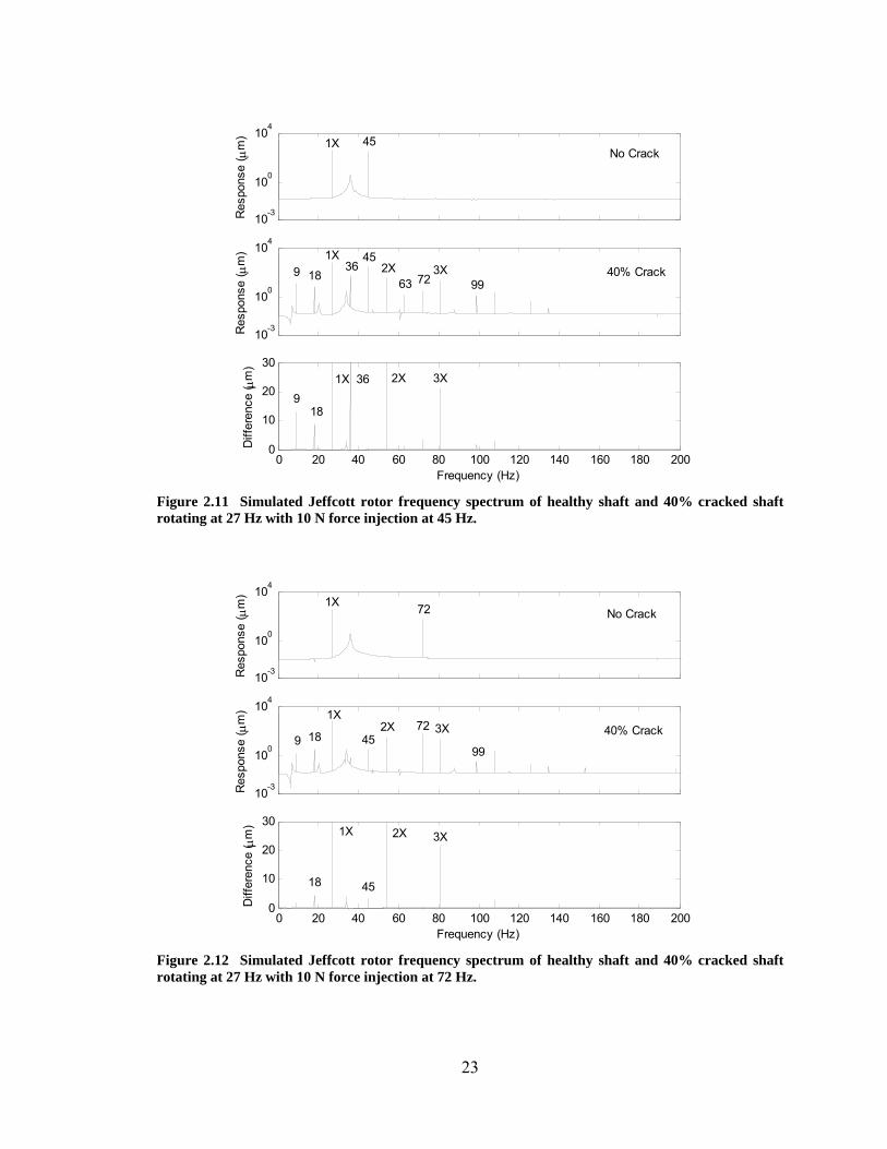
Figure 2.11 Simulated Jeffcott rotor frequency spectrum of healthy shaft and 40% cracked shaft rotating at 27 Hz with 10 N force injection at 45 Hz.
10-3
100
104
Res
pons
e ( μ
m)
10-3
100
104
Res
pons
e ( μ
m)
0 20 40 60 80 100 120 140 160 180 2000
10
20
30
Diff
eren
ce ( μ
m)
Frequency (Hz)
No Crack
40% Crack
1X
1X 2X 3X
1X 2X 3X
9 18 4572
99
18 45
72
Figure 2.12 Simulated Jeffcott rotor frequency spectrum of healthy shaft and 40% cracked shaft rotating at 27 Hz with 10 N force injection at 72 Hz.
23
CHAPTER III
THE CRACK DETECTION TEST RIG
3.1 Overview of the Test Rig
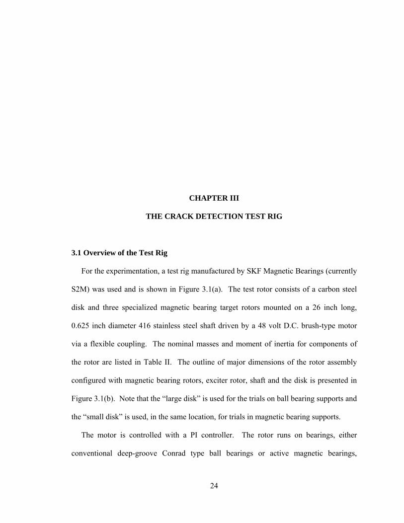
For the experimentation, a test rig manufactured by SKF Magnetic Bearings (currently
S2M) was used and is shown in Figure 3.1(a). The test rotor consists of a carbon steel
disk and three specialized magnetic bearing target rotors mounted on a 26 inch long,
0.625 inch diameter 416 stainless steel shaft driven by a 48 volt D.C. brush-type motor
via a flexible coupling. The nominal masses and moment of inertia for components of
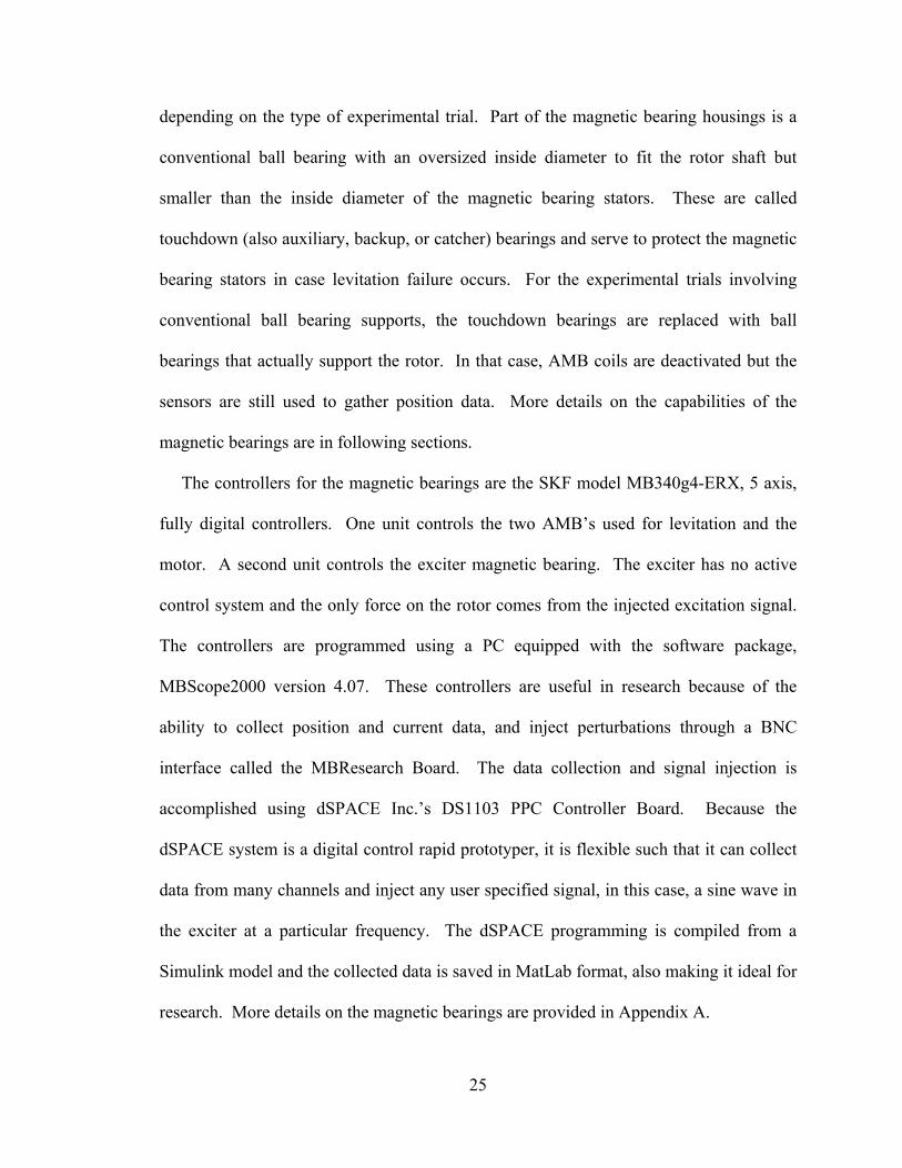
the rotor are listed in Table II. The outline of major dimensions of the rotor assembly
configured with magnetic bearing rotors, exciter rotor, shaft and the disk is presented in
Figure 3.1(b). Note that the “large disk” is used for the trials on ball bearing supports and
the “small disk” is used, in the same location, for trials in magnetic bearing supports.
The motor is controlled with a PI controller. The rotor runs on bearings, either
conventional deep-groove Conrad type ball bearings or active magnetic bearings,
24
depending on the type of experimental trial. Part of the magnetic bearing housings is a
conventional ball bearing with an oversized inside diameter to fit the rotor shaft but
smaller than the inside diameter of the magnetic bearing stators. These are called
touchdown (also auxiliary, backup, or catcher) bearings and serve to protect the magnetic
bearing stators in case levitation failure occurs. For the experimental trials involving
conventional ball bearing supports, the touchdown bearings are replaced with ball
bearings that actually support the rotor. In that case, AMB coils are deactivated but the
sensors are still used to gather position data. More details on the capabilities of the
magnetic bearings are in following sections.
The controllers for the magnetic bearings are the SKF model MB340g4-ERX, 5 axis,
fully digital controllers. One unit controls the two AMB’s used for levitation and the
motor. A second unit controls the exciter magnetic bearing. The exciter has no active
control system and the only force on the rotor comes from the injected excitation signal.
The controllers are programmed using a PC equipped with the software package,
MBScope2000 version 4.07. These controllers are useful in research because of the
ability to collect position and current data, and inject perturbations through a BNC
interface called the MBResearch Board. The data collection and signal injection is
accomplished using dSPACE Inc.’s DS1103 PPC Controller Board. Because the
dSPACE system is a digital control rapid prototyper, it is flexible such that it can collect
data from many channels and inject any user specified signal, in this case, a sine wave in
the exciter at a particular frequency. The dSPACE programming is compiled from a
Simulink model and the collected data is saved in MatLab format, also making it ideal for
research. More details on the magnetic bearings are provided in Appendix A.
25
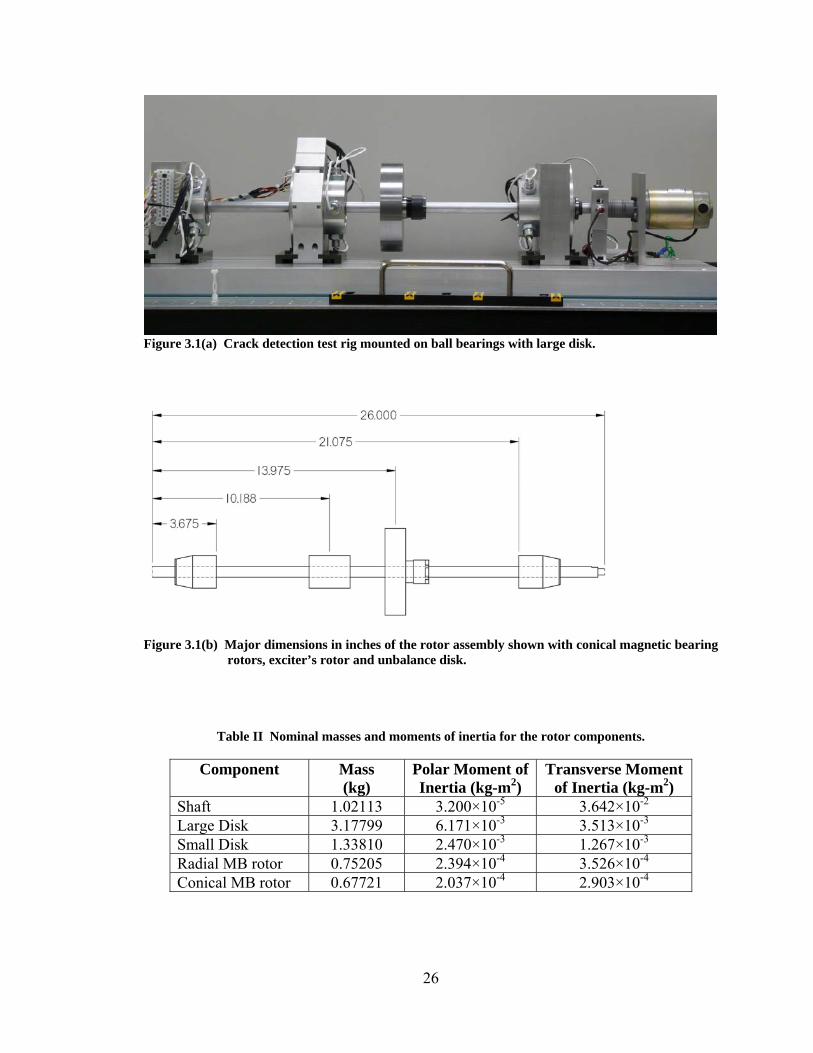
Figure 3.1(a) Crack detection test rig mounted on ball bearings with large disk.
Figure 3.1(b) Major dimensions in inches of the rotor assembly shown with conical magnetic bearing
rotors, exciter’s rotor and unbalance disk.
Table II Nominal masses and moments of inertia for the rotor components.
Component Mass (kg)
Polar Moment of Inertia (kg-m2)
Transverse Moment of Inertia (kg-m2)
Shaft 1.02113 3.200×10⁻⁵ 3.642×10⁻² Large Disk 3.17799 6.171×10⁻³ 3.513×10⁻³ Small Disk 1.33810 2.470×10⁻³ 1.267×10⁻³ Radial MB rotor 0.75205 2.394×10⁻⁴ 3.526×10⁻⁴ Conical MB rotor 0.67721 2.037×10⁻⁴ 2.903×10⁻⁴
26
3.2 Overview of Active Magnetic Bearings: Modeling and Control
3.2.1 One-Axis Control
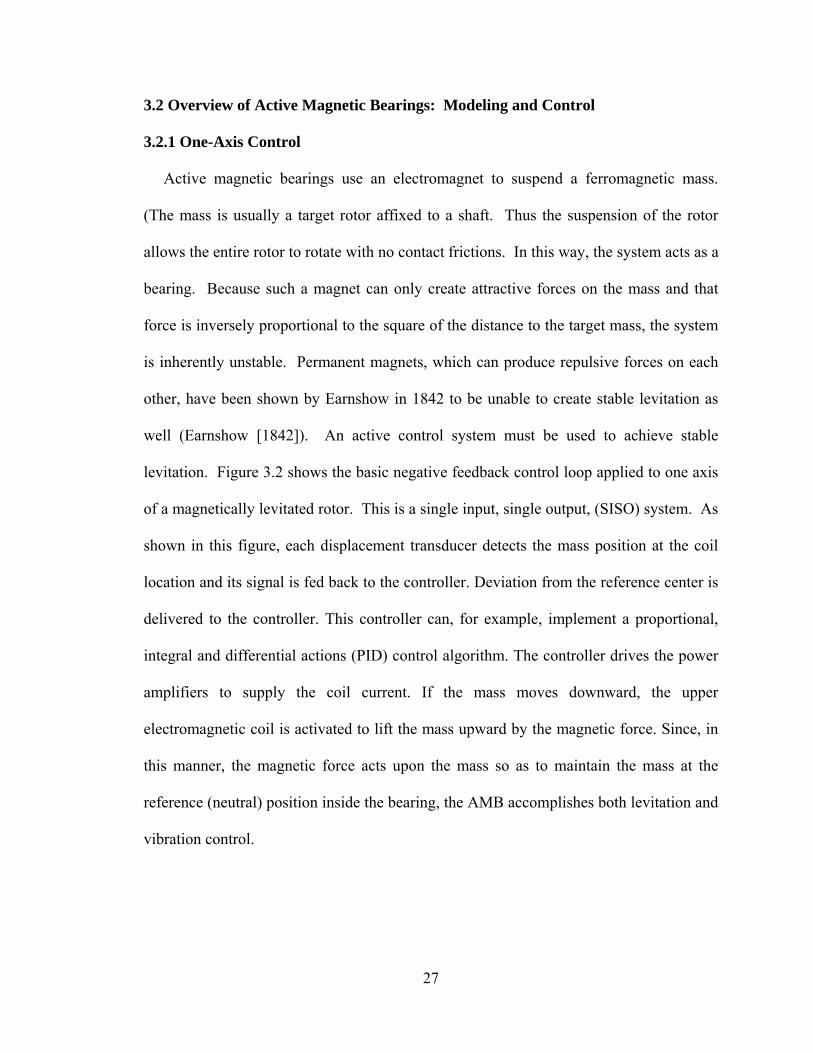
Active magnetic bearings use an electromagnet to suspend a ferromagnetic mass.
(The mass is usually a target rotor affixed to a shaft. Thus the suspension of the rotor
allows the entire rotor to rotate with no contact frictions. In this way, the system acts as a
bearing. Because such a magnet can only create attractive forces on the mass and that
force is inversely proportional to the square of the distance to the target mass, the system
is inherently unstable. Permanent magnets, which can produce repulsive forces on each
other, have been shown by Earnshow in 1842 to be unable to create stable levitation as
well (Earnshow [1842]). An active control system must be used to achieve stable
levitation. Figure 3.2 shows the basic negative feedback control loop applied to one axis
of a magnetically levitated rotor. This is a single input, single output, (SISO) system. As
shown in this figure, each displacement transducer detects the mass position at the coil
location and its signal is fed back to the controller. Deviation from the reference center is
delivered to the controller. This controller can, for example, implement a proportional,
integral and differential actions (PID) control algorithm. The controller drives the power
amplifiers to supply the coil current. If the mass moves downward, the upper
electromagnetic coil is activated to lift the mass upward by the magnetic force. Since, in
this manner, the magnetic force acts upon the mass so as to maintain the mass at the
reference (neutral) position inside the bearing, the AMB accomplishes both levitation and
vibration control.
27
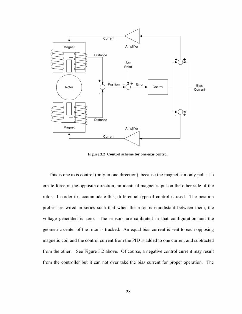
Figure 3.2 Control scheme for one-axis control.
This is one axis control (only in one direction), because the magnet can only pull. To
create force in the opposite direction, an identical magnet is put on the other side of the
rotor. In order to accommodate this, differential type of control is used. The position
probes are wired in series such that when the rotor is equidistant between them, the
voltage generated is zero. The sensors are calibrated in that configuration and the
geometric center of the rotor is tracked. An equal bias current is sent to each opposing
magnetic coil and the control current from the PID is added to one current and subtracted
from the other. See Figure 3.2 above. Of course, a negative control current may result
from the controller but it can not over take the bias current for proper operation. The
28
resulting force from the opposing magnets can now be positive or negative and can be
controlled.
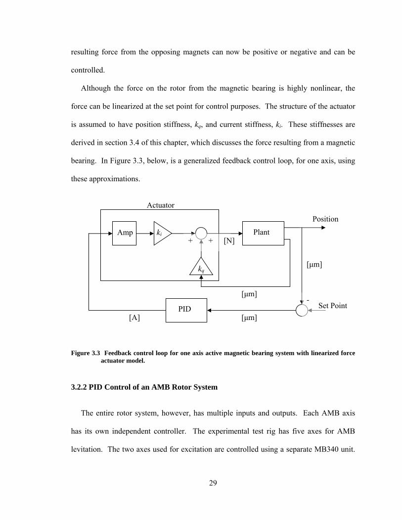
Although the force on the rotor from the magnetic bearing is highly nonlinear, the
force can be linearized at the set point for control purposes. The structure of the actuator
is assumed to have position stiffness, kq, and current stiffness, ki. These stiffnesses are
derived in section 3.4 of this chapter, which discusses the force resulting from a magnetic
bearing. In Figure 3.3, below, is a generalized feedback control loop, for one axis, using
these approximations.
Actuator Amp ki kq
PID
Plant
Position
+ +
[μm] [A]
[μm]
[μm]
[N]
- Set Point
Figure 3.3 Feedback control loop for one axis active magnetic bearing system with linearized force actuator model.
3.2.2 PID Control of an AMB Rotor System
The entire rotor system, however, has multiple inputs and outputs. Each AMB axis
has its own independent controller. The experimental test rig has five axes for AMB
levitation. The two axes used for excitation are controlled using a separate MB340 unit.
29
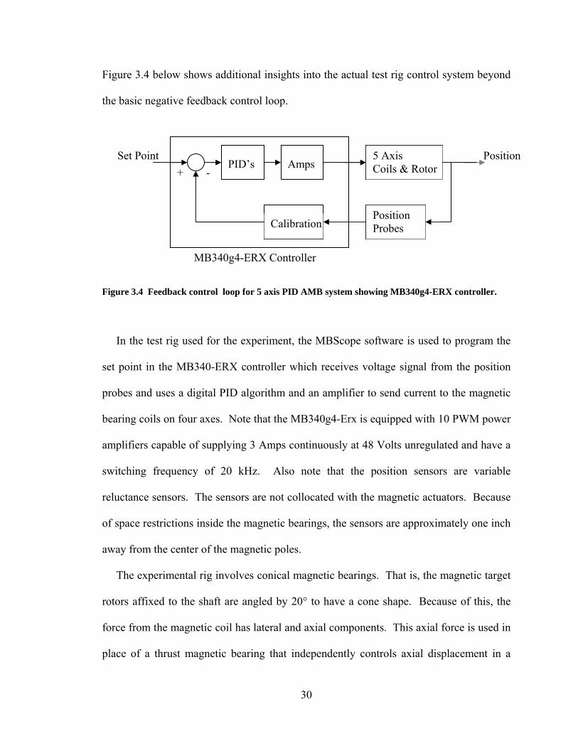
Figure 3.4 below shows additional insights into the actual test rig control system beyond
the basic negative feedback control loop.
+ - Set Point
PID’s
MB340g4-ERX Controller
Amps
Calibration Position Probes
Position 5 Axis Coils & Rotor
Figure 3.4 Feedback control loop for 5 axis PID AMB system showing MB340g4-ERX controller.
In the test rig used for the experiment, the MBScope software is used to program the
set point in the MB340-ERX controller which receives voltage signal from the position
probes and uses a digital PID algorithm and an amplifier to send current to the magnetic
bearing coils on four axes. Note that the MB340g4-Erx is equipped with 10 PWM power
amplifiers capable of supplying 3 Amps continuously at 48 Volts unregulated and have a
switching frequency of 20 kHz. Also note that the position sensors are variable
reluctance sensors. The sensors are not collocated with the magnetic actuators. Because
of space restrictions inside the magnetic bearings, the sensors are approximately one inch
away from the center of the magnetic poles.
The experimental rig involves conical magnetic bearings. That is, the magnetic target
rotors affixed to the shaft are angled by 20° to have a cone shape. Because of this, the
force from the magnetic coil has lateral and axial components. This axial force is used in
place of a thrust magnetic bearing that independently controls axial displacement in a
30
normal radial (not axial) magnetic bearing. In this way, five independent control loops
use four magnetic bearing coil pairs to control position in five axes. For more
background on magnetic bearings, see Schweitzer [1994] and Maslen [2000].
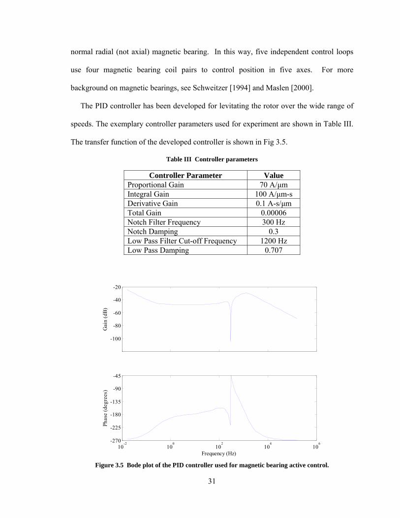
The PID controller has been developed for levitating the rotor over the wide range of
speeds. The exemplary controller parameters used for experiment are shown in Table III.
The transfer function of the developed controller is shown in Fig 3.5.
Table III Controller parameters
Controller Parameter Value Proportional Gain 70 A/μm Integral Gain 100 A/μm-s Derivative Gain 0.1 A-s/μm Total Gain 0.00006 Notch Filter Frequency 300 Hz Notch Damping 0.3 Low Pass Filter Cut-off Frequency 1200 Hz Low Pass Damping 0.707
-100
-80
-60
-40
-20
Gai
n (d
B)
10-2
100
102
104
106-270
-225
-180
-135
-90
-45
Phas
e (d
egre
es)
Frequency (Hz)
Figure 3.5 Bode plot of the PID controller used for magnetic bearing active control.
31
3.3 Rotordynamic Modeling
Finite element approach was applied in modeling of rotor-bearing system. The rotor
was discretized into finite elements using Timoshenko beam elements. The finite
element modeling program, XLRotor version 3.52 by Rotating Machinery Analysis Inc.,
was used. The rotordynamic analysis involves generation of the Campbell Diagram and
calculation of critical speeds and mode shapes for the rotor on ball bearings and active
magnetic bearings. Also included is the prediction of static deflection of the rotor and the
critical speed map. For detailed geometry of the rotors, see XLRotor input files in
Appendix B.
3.3.1 Conventional Bearing Supports
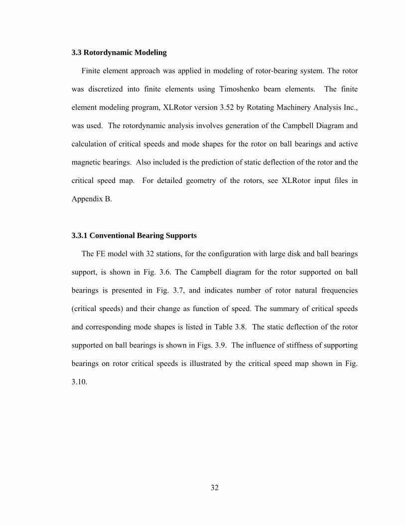
The FE model with 32 stations, for the configuration with large disk and ball bearings
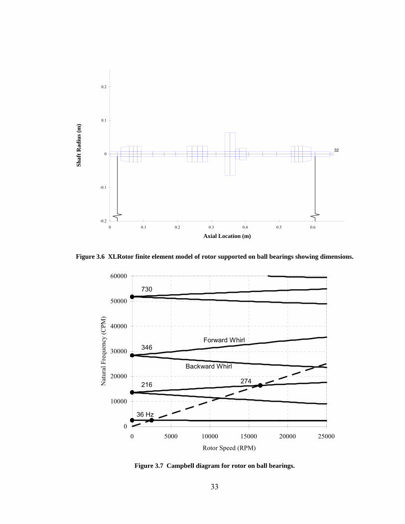
support, is shown in Fig. 3.6. The Campbell diagram for the rotor supported on ball
bearings is presented in Fig. 3.7, and indicates number of rotor natural frequencies
(critical speeds) and their change as function of speed. The summary of critical speeds
and corresponding mode shapes is listed in Table 3.8. The static deflection of the rotor
supported on ball bearings is shown in Figs. 3.9. The influence of stiffness of supporting
bearings on rotor critical speeds is illustrated by the critical speed map shown in Fig.
3.10.
32
32
-0.2
-0.1
0
0.1
0.2
0 0.1 0.2 0.3 0.4 0.5 0.6
Axial Location (m)
Shaf
t Rad
ius (
m)
Figure 3.6 XLRotor finite element model of rotor supported on ball bearings showing dimensions.
0
10000
20000
30000
40000
50000
60000
0 5000 10000 15000 20000 25000
Rotor Speed (RPM)
Nat
ural
Fre
quen
cy (C
PM)
36 Hz
216 274
346
730
Forward Whirl
Backward Whirl
Figure 3.7 Campbell diagram for rotor on ball bearings.
33
The Campbell diagram is a graph of natural frequency as a function of running speed.
As the rotor speeds up, gyroscopic effects cause an affective stiffening of the rotor which
in turn causes a change in natural frequency. Significant change in natural frequency
occurs in modes that have significant tilting at disks. The dashed line has a slope of 1.
The critical speed can be read at the intersection point of a unity-slope line with the
forward branch of each natural frequency.
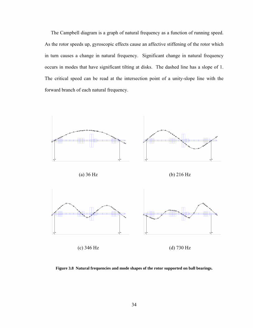
(a) 36 Hz (b) 216 Hz
(c) 346 Hz (d) 730 Hz
Figure 3.8 Natural frequencies and mode shapes of the rotor supported on ball bearings.
34
The maximum running speed of the test rig is 15000 RPM (250 Hz). Only the first
mode can be excited in this range. Note that the second mode changes natural frequency
significantly because of the tilting of the disk where as the first mode natural frequency is
nearly unchanged.
32
-0.2
-0.1
0
0.1
0.2
0 0.1 0.2 0.3 0.4 0.5 0.6
Axial Location (m)
Shaf
t Rad
ius (
m)
-0.2
-0.15
-0.1
-0.05
0
0.05
0.1
0.15
0.2
0.25
Stat
ic D
efle
ctio
n (m
m p
k)
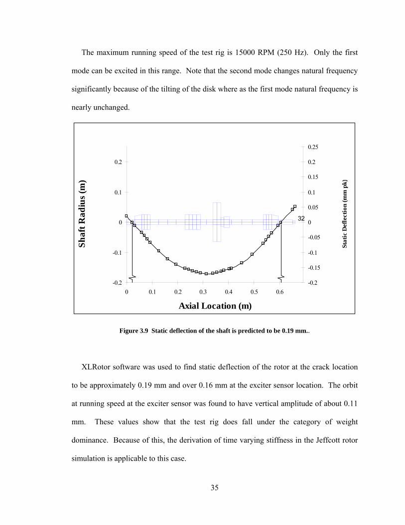
Figure 3.9 Static deflection of the shaft is predicted to be 0.19 mm..
XLRotor software was used to find static deflection of the rotor at the crack location
to be approximately 0.19 mm and over 0.16 mm at the exciter sensor location. The orbit
at running speed at the exciter sensor was found to have vertical amplitude of about 0.11
mm. These values show that the test rig does fall under the category of weight
dominance. Because of this, the derivation of time varying stiffness in the Jeffcott rotor
simulation is applicable to this case.
35
1
10
100
1000
10000
100000
1000000
1. 10. 100. 1000. 10000. 100000. 1000000. 10000000.
Bearing Stiffness (N/m)
Crit
ical
Spe
ed (C
PM)
Figure 3.10 Undamped critical speed map showing critical speed as a function of bearing stiffness.
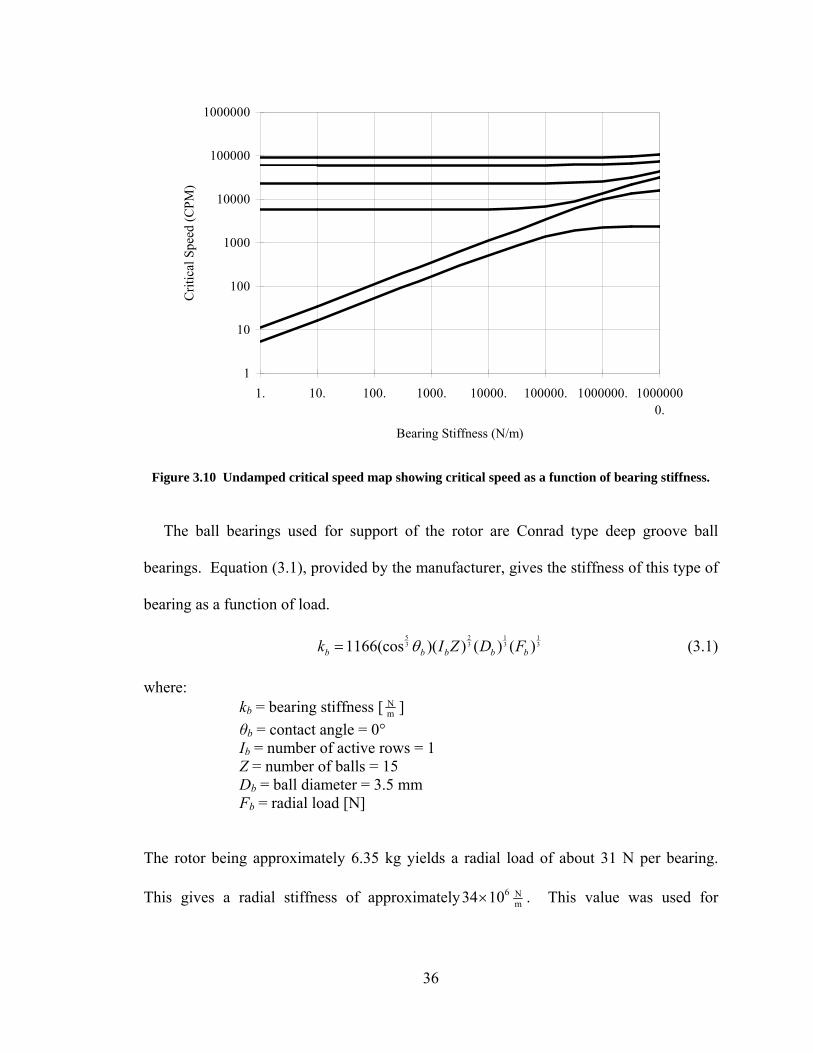
The ball bearings used for support of the rotor are Conrad type deep groove ball
bearings. Equation (3.1), provided by the manufacturer, gives the stiffness of this type of
bearing as a function of load.
5 2 13 3 31166(cos )( ) ( ) ( )b b b bk I Z Dθ=
13
bF (3.1)
where: kb = bearing stiffness [ N
m ] θb = contact angle = 0° Ib = number of active rows = 1 Z = number of balls = 15 Db = ball diameter = 3.5 mm Fb = radial load [N]
The rotor being approximately 6.35 kg yields a radial load of about 31 N per bearing.
This gives a radial stiffness of approximately 6 Nm34 10× . This value was used for
36
modeling. Also, a value of N-sm10 was assumed for damping and cross coupling of
stiffness and damping was neglected.
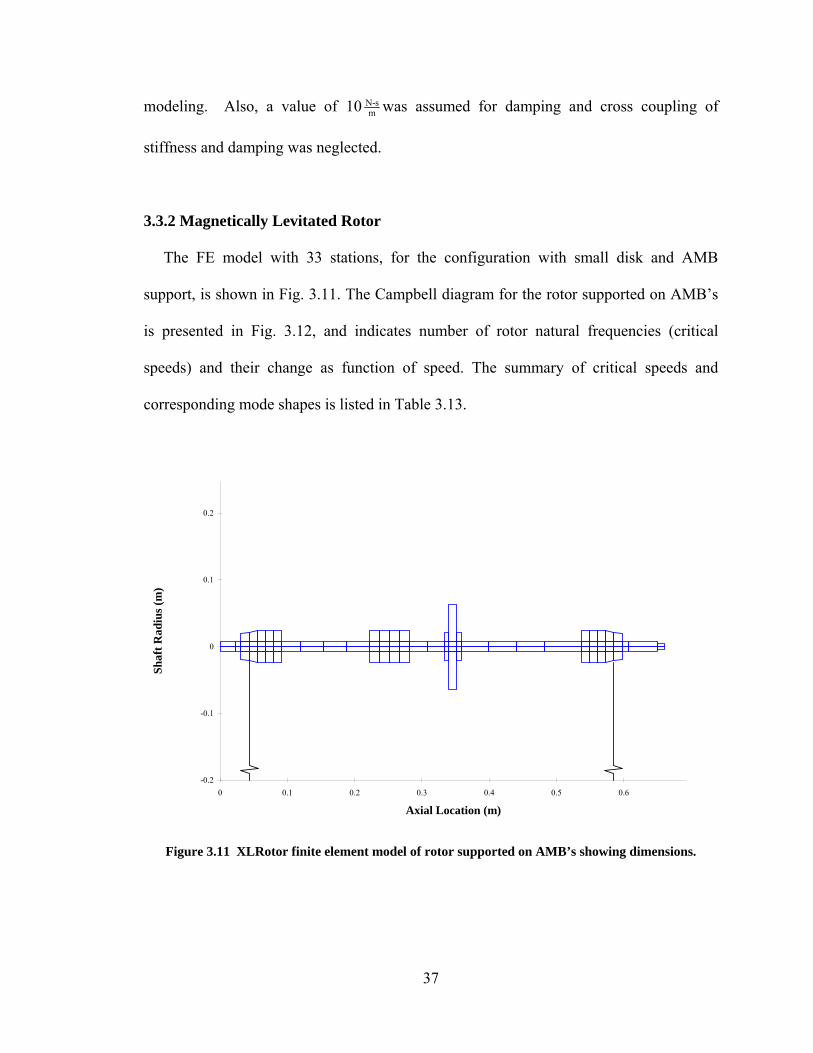
3.3.2 Magnetically Levitated Rotor
The FE model with 33 stations, for the configuration with small disk and AMB
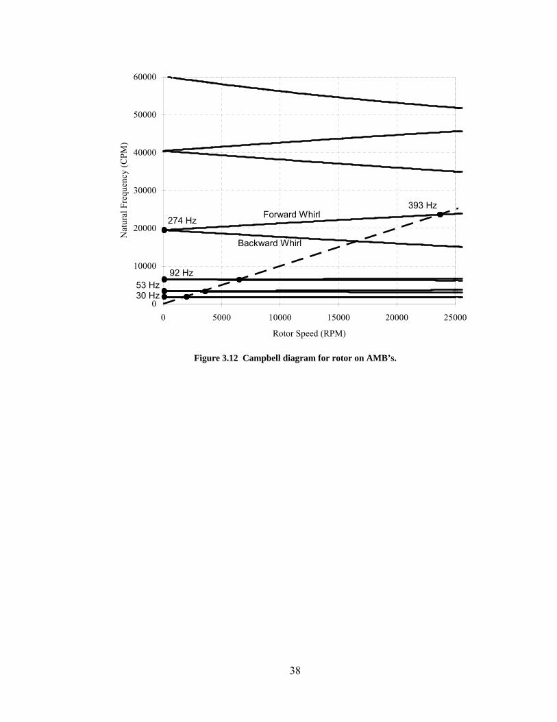
support, is shown in Fig. 3.11. The Campbell diagram for the rotor supported on AMB’s
is presented in Fig. 3.12, and indicates number of rotor natural frequencies (critical
speeds) and their change as function of speed. The summary of critical speeds and
corresponding mode shapes is listed in Table 3.13.
-0.2
-0.1
0
0.1
0.2
0 0.1 0.2 0.3 0.4 0.5 0.6
Axial Location (m)
Shaf
t Rad
ius (
m)
Figure 3.11 XLRotor finite element model of rotor supported on AMB’s showing dimensions.
37
0
10000
20000
30000
40000
50000
60000
0 5000 10000 15000 20000 25000
Rotor Speed (RPM)
Nat
ural
Fre
quen
cy (C
PM)
30 Hz53 Hz
92 Hz
274 Hz
393 HzForward Whirl
Backward Whirl
Figure 3.12 Campbell diagram for rotor on AMB’s.
38
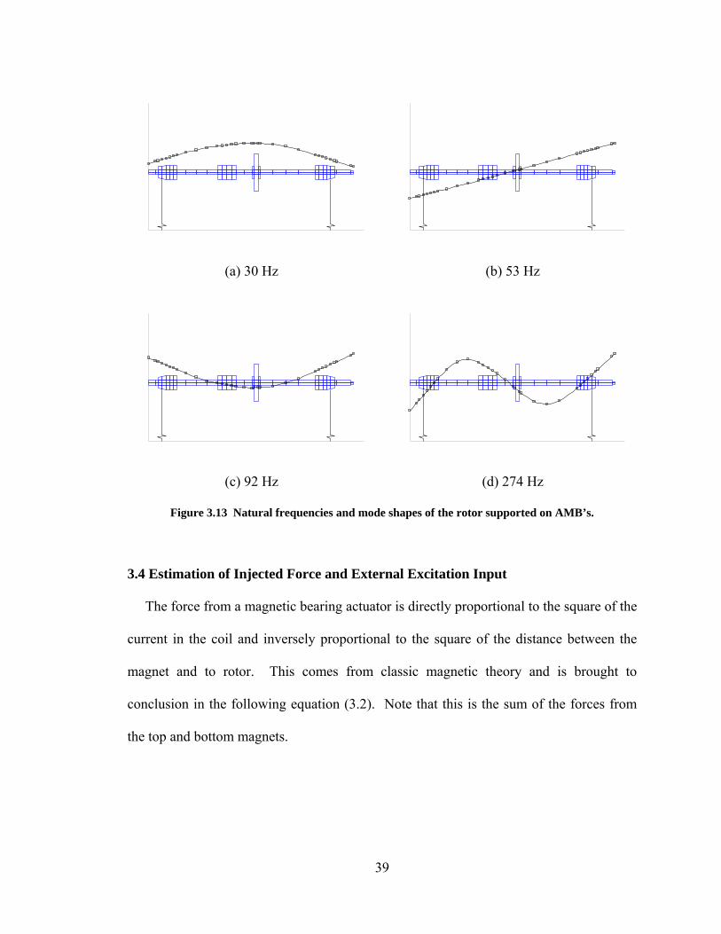
(a) 30 Hz (b) 53 Hz
(c) 92 Hz (d) 274 Hz
Figure 3.13 Natural frequencies and mode shapes of the rotor supported on AMB’s.
3.4 Estimation of Injected Force and External Excitation Input
The force from a magnetic bearing actuator is directly proportional to the square of the
current in the coil and inversely proportional to the square of the distance between the
magnet and to rotor. This comes from classic magnetic theory and is brought to
conclusion in the following equation (3.2). Note that this is the sum of the forces from
the top and bottom magnets.
39
( ) ( )
2 2
2 2top bottom
ap ap
I IF Cg q g q
⎡ ⎤⎛ ⎞ ⎛ ⎞⎢ ⎥⎜ ⎟ ⎜= − ⎟⎢ ⎥⎜ ⎟ ⎜− +⎝ ⎠ ⎝
⎟⎠⎣ ⎦
(3.2)
Here: F = force [N] C = force calibration factor [
2
2N-μm
A]
Itop = current in the top coil [A] I = current in the bottom coil [A] bottom g = effective gap between the magnet and the rotor = 401.55 μm ap q = displacement of the rotor [μm]
The linearized stiffnesses used for the feedback control loop can be found by taking
the partial derivative of the force equation with respect to displacement, x, and control
current. The top current is the sum of the control current and the bias current and the
bottom current is the difference between them.
2 2
2
( ) (4( ) 4( )bias control bias control
ap ap
I I I IF Cg q g q 2
)⎡ ⎤+ −= −⎢ ⎥
− +⎢ ⎥⎣ ⎦ (3.3)
2 2
3 3
( ) (( 2)( 1) ( 2)(1)4( ) 4( )bias control bias control
qap ap
I I I IFk Cq g q g
⎡ ⎤+∂≡ = − − − −⎢ ⎥∂ −⎢ ⎥⎣ ⎦
)q
−+
(3.4)
2 2
( ) ((2)(1) (2)( 1)4( ) 4( )bias control bias control
icontrol ap ap
I I I IFk CI g q g
)q
⎡ ⎤+ −∂≡ = − −⎢ ⎥
∂ − +⎢ ⎥⎣ ⎦ (3.5)
In this case, the set point is the center of the bearing, so the equation is linearized around
x = 0. And, with no deflection, Icontrol = 0. Making these substitutions, the equations can
be simplified to:
2
3bias
qap
CIkg
= (3.6)
2bias
iap
CIkg
= (3.7)
40
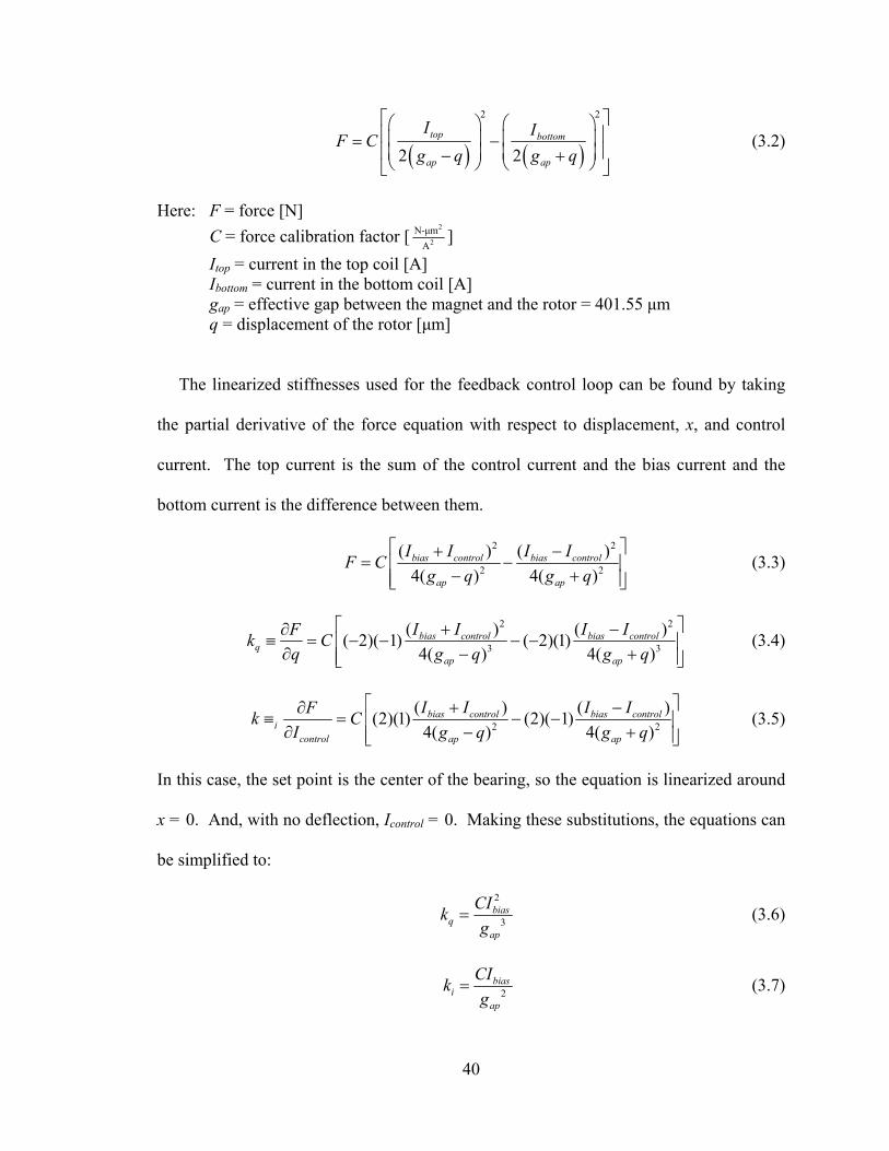
The calibration factor, C, is theoretically given by equation (3.8):
20 cos( )C ANμ α= (3.8)
With μ0 being the permeability of a vacuum (4π×10-7 Hm ), A being the area of a pole face,
N being the number of windings in a coil and α being the angle of the pole face. See
Plonus [1978] for a derivation of equation (3.8) and a thorough explanation of the force
generated by an electromagnet.
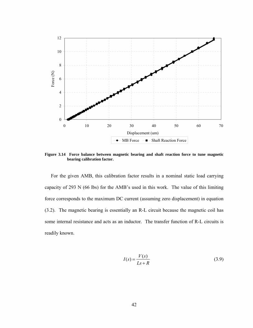
The value of C in equation (3.2) was experimentally determined to be C = 212
2N-μm
A.
This was accomplished by the measurement of the stiffness of the rotor and then
matching it with the slope of the force-displacement relationship curve which obtained
experimentally. In other words, the displacement of the shaft in response to known
forces was measured and plotted below. Then, the displacement of the MB rotor in
response to known currents was measured. Then, Equation (3.2) was used to plot force-
displacement relationship on the same plot and the value of C was tuned so the curves
would coincide.
41
0
2
4
6
8
10
12
0 10 20 30 40 50 60 7
Displacement (um)
Forc
e (N
)
0
MB Force Shaft Reaction Force
Figure 3.14 Force balance between magnetic bearing and shaft reaction force to tune magnetic
bearing calibration factor.
For the given AMB, this calibration factor results in a nominal static load carrying
capacity of 293 N (66 lbs) for the AMB’s used in this work. The value of this limiting
force corresponds to the maximum DC current (assuming zero displacement) in equation
(3.2). The magnetic bearing is essentially an R-L circuit because the magnetic coil has
some internal resistance and acts as an inductor. The transfer function of R-L circuits is
readily known.
( )( ) V sI sLs R
=+
(3.9)
42
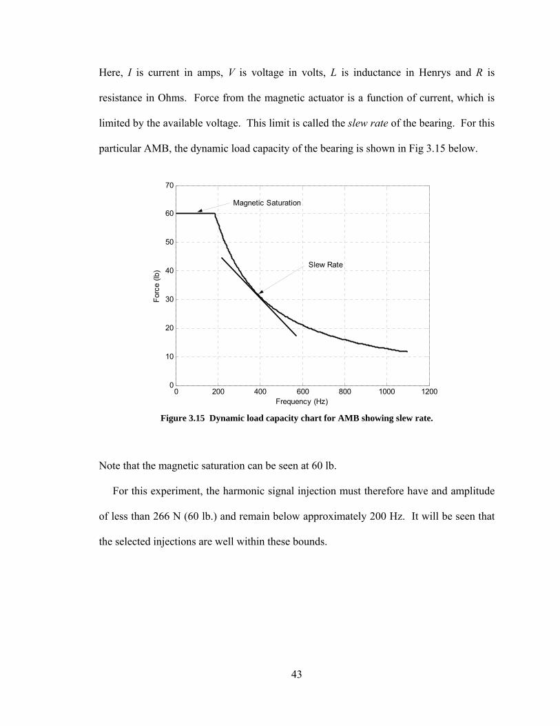
Here, I is current in amps, V is voltage in volts, L is inductance in Henrys and R is
resistance in Ohms. Force from the magnetic actuator is a function of current, which is
limited by the available voltage. This limit is called the slew rate of the bearing. For this
particular AMB, the dynamic load capacity of the bearing is shown in Fig 3.15 below.
0 200 400 600 800 1000 12000
10
20
30
40
50
60
70
Frequency (Hz)
Forc
e (lb
)
Magnetic Saturation
Slew Rate
Figure 3.15 Dynamic load capacity chart for AMB showing slew rate.
Note that the magnetic saturation can be seen at 60 lb.
For this experiment, the harmonic signal injection must therefore have and amplitude
of less than 266 N (60 lb.) and remain below approximately 200 Hz. It will be seen that
the selected injections are well within these bounds.
43
CHAPTER IV
DAMAGE DETECTION: EXPERIMENTAL RESULTS
4.1 Introduction
As previously stated, there are two parts to this experiment, damage detection for a
rotor on ball bearing supports and damage detection for a magnetically levitated rotor.
For each, an undamaged (healthy) rotor is run at steady state and vibration data collected.
Then the rotor is run again with a harmonic current input to a magnetic bearing and the
position data collected. The exciter magnetic bearing is used for force injection in the
vertical axis in the ball bearing trials. The outboard AMB (furthest from the motor) is
used to inject harmonic force at 45° in the magnetic levitation trials. The integers 2, 3,
and 4 are selected as n values in equation (2.14) to calculate force injection frequencies.
The frequency spectrum is found for each set of position data sets by using the FFT
algorithm. The same force injection cases are repeated with rotor shafts intentionally
damaged with a wire EDM cut at the bearing midspan. The wire EDM cut is
44
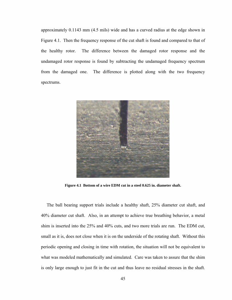
approximately 0.1143 mm (4.5 mils) wide and has a curved radius at the edge shown in
Figure 4.1. Then the frequency response of the cut shaft is found and compared to that of
the healthy rotor. The difference between the damaged rotor response and the
undamaged rotor response is found by subtracting the undamaged frequency spectrum
from the damaged one. The difference is plotted along with the two frequency
spectrums.
Figure 4.1 Bottom of a wire EDM cut in a steel 0.625 in. diameter shaft.
The ball bearing support trials include a healthy shaft, 25% diameter cut shaft, and
40% diameter cut shaft. Also, in an attempt to achieve true breathing behavior, a metal
shim is inserted into the 25% and 40% cuts, and two more trials are run. The EDM cut,
small as it is, does not close when it is on the underside of the rotating shaft. Without this
periodic opening and closing in time with rotation, the situation will not be equivalent to
what was modeled mathematically and simulated. Care was taken to assure that the shim
is only large enough to just fit in the cut and thus leave no residual stresses in the shaft.
45
This is a total of 20 cases and 16 comparisons. For each, data is collected for 30 seconds
at 10 kHz and the frequency spectrum of 4 data collections is averaged.
The magnetic levitation trials include only a 40% diameter EDM cut shaft and healthy
shaft rotors. These cases prove sufficient in demonstrating the crack detection method is
viable for magnetically levitated rotors. This gives a total of 8 cases and 4 comparisons.
For each, data is again collected for 30 seconds at 10 kHz but the frequency spectrum of
18 data collections is averaged.
4.2 Conventional Bearing Support
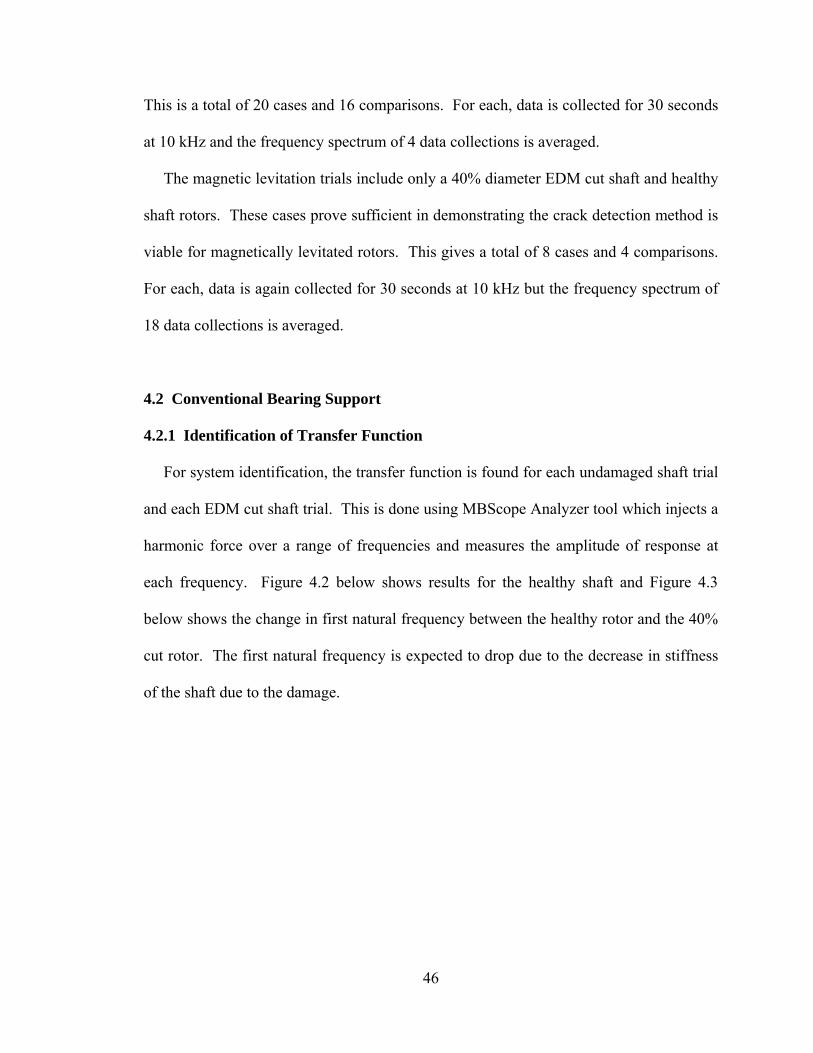
4.2.1 Identification of Transfer Function
For system identification, the transfer function is found for each undamaged shaft trial
and each EDM cut shaft trial. This is done using MBScope Analyzer tool which injects a
harmonic force over a range of frequencies and measures the amplitude of response at
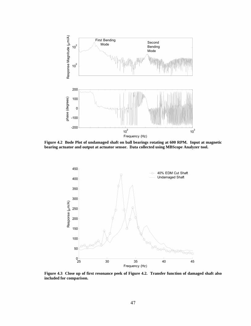
each frequency. Figure 4.2 below shows results for the healthy shaft and Figure 4.3
below shows the change in first natural frequency between the healthy rotor and the 40%
cut rotor. The first natural frequency is expected to drop due to the decrease in stiffness
of the shaft due to the damage.
46
100
102
Res
pons
e M
agni
tude
( μm
/A)
102 103-200
-100
0
100
200
Frequency (Hz)
phas
e (d
egre
es)
First Bending Mode Second
BendingMode
Figure 4.2 Bode Plot of undamaged shaft on ball bearings rotating at 600 RPM. Input at magnetic bearing actuator and output at actuator sensor. Data collected using MBScope Analyzer tool.
25 30 35 40 450
50
100
150
200
250
300
350
400
450
Frequency (Hz)
Res
pons
e ( μ
m/A
)
40% EDM Cut ShaftUndamaged Shaft
Figure 4.3 Close up of first resonance peek of Figure 4.2. Transfer function of damaged shaft also included for comparison.
47
4.2.2 Experimental Results: Healthy and Damaged Rotor
A harmonic current is input to the exciter magnetic bearing however, as shown in
equation (3.2), the resulting force on the rotor is a function of both current and rotor
position. Figure 4.4 below shows the actual periodic force injected to the system as
calculated by equation (3.2). The main frequency in the injection force is the current
injection frequency. Figure 4.4 also includes the values of the injection frequencies and
magnitudes. Note that higher injection amplitudes are possible because the mass of the
rotor is of course a second order system and the deflection is less at higher frequencies.
-20
0
20
Forc
e (N
)
-20
0
20
Forc
e (N
)
-50
0
50
Forc
e (N
)
0 0.05 0.1 0.15 0.2 0.25 0.3 0.35 0.4 0.45 0.5-100
0
100
Time (s)
Forc
e (N
)
No Injection
0.25 A at 18 Hz
0.274 A at 45 Hz
0.479 A at 72 Hz
Figure 4.4 Example of four force injection cases for ball bearing trials calculated from experimental current and position data using equation (3.2).
Figures 4.5 through 4.8 show the four injection cases for the 25% diameter EDM cut
shaft. In Figure 4.5 where there is no damage and no injection, there is a large peek at
one times running speed due to unbalance which causes a synchronous force. Also
48
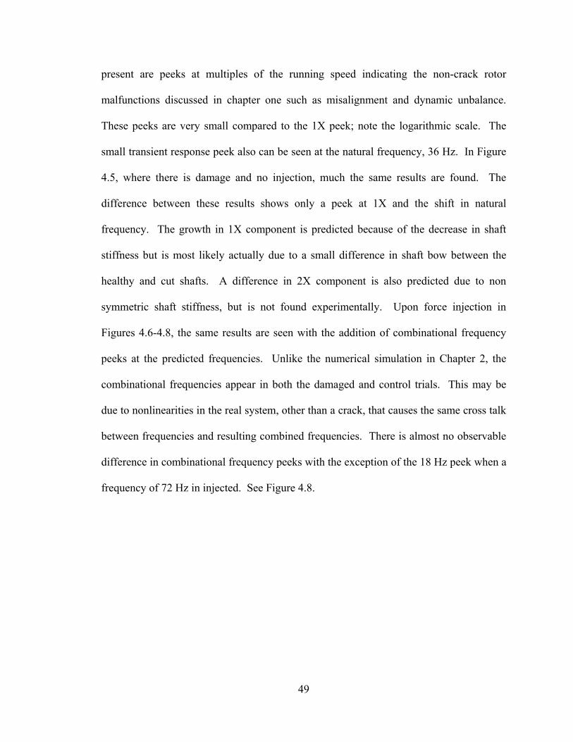
present are peeks at multiples of the running speed indicating the non-crack rotor
malfunctions discussed in chapter one such as misalignment and dynamic unbalance.
These peeks are very small compared to the 1X peek; note the logarithmic scale. The
small transient response peek also can be seen at the natural frequency, 36 Hz. In Figure
4.5, where there is damage and no injection, much the same results are found. The
difference between these results shows only a peek at 1X and the shift in natural
frequency. The growth in 1X component is predicted because of the decrease in shaft
stiffness but is most likely actually due to a small difference in shaft bow between the
healthy and cut shafts. A difference in 2X component is also predicted due to non
symmetric shaft stiffness, but is not found experimentally. Upon force injection in
Figures 4.6-4.8, the same results are seen with the addition of combinational frequency
peeks at the predicted frequencies. Unlike the numerical simulation in Chapter 2, the
combinational frequencies appear in both the damaged and control trials. This may be
due to nonlinearities in the real system, other than a crack, that causes the same cross talk
between frequencies and resulting combined frequencies. There is almost no observable
difference in combinational frequency peeks with the exception of the 18 Hz peek when a
frequency of 72 Hz in injected. See Figure 4.8.
49
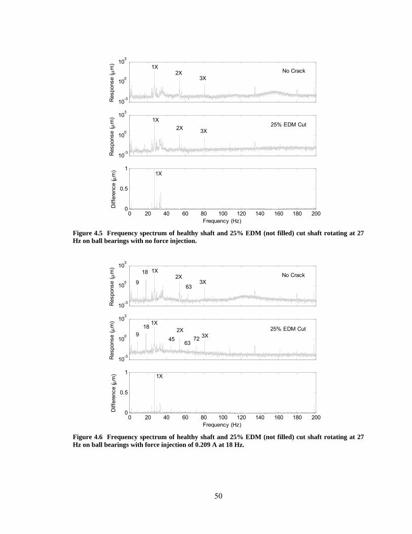
10-3
100
103
Res
pons
e ( μ
m)
10-3
100
103R
espo
nse
( μm
)
0 20 40 60 80 100 120 140 160 180 2000
0.5
1
Diff
eren
ce ( μ
m)
Frequency (Hz)
1X 2X
3X No Crack
25% EDM Cut 1X
2X 3X
1X
Figure 4.5 Frequency spectrum of healthy shaft and 25% EDM (not filled) cut shaft rotating at 27 Hz on ball bearings with no force injection.
10-3
100
103
Res
pons
e ( μ
m)
10-3
100
103
Res
pons
e ( μ
m)
0 20 40 60 80 100 120 140 160 180 2000
0.5
1
Diff
eren
ce ( μ
m)
Frequency (Hz)
25% EDM Cut
No Crack 3X
2X 1X
9 18
1X
45 2X
63 72 3X
63
18
9
1X
Figure 4.6 Frequency spectrum of healthy shaft and 25% EDM (not filled) cut shaft rotating at 27 Hz on ball bearings with force injection of 0.209 A at 18 Hz.
50
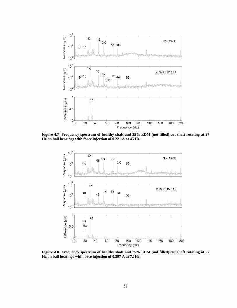
10-3
100
103
Res
pons
e ( μ
m)
10-3
100
103R
espo
nse
( μm
)
0 20 40 60 80 100 120 140 160 180 2000
0.5
1
Diff
eren
ce ( μ
m)
Frequency (Hz)
25% EDM Cut
No Crack 3X
2X 1X
9 18
1X 45
2X 63
72 3X 99
1X
9 18
45 72
Figure 4.7 Frequency spectrum of healthy shaft and 25% EDM (not filled) cut shaft rotating at 27 Hz on ball bearings with force injection of 0.221 A at 45 Hz.
10-3
100
103
Res
pons
e ( μ
m)
10-3
100
103
Res
pons
e ( μ
m)
0 20 40 60 80 100 120 140 160 180 2000
0.5
1
Diff
eren
ce ( μ
m)
Frequency (Hz)
25% EDM Cut
No Crack 3X
2X 1X
1845 72
99
18
1X
452X 72 3X
99
18 Hz
1X
Figure 4.8 Frequency spectrum of healthy shaft and 25% EDM (not filled) cut shaft rotating at 27 Hz on ball bearings with force injection of 0.297 A at 72 Hz.
51
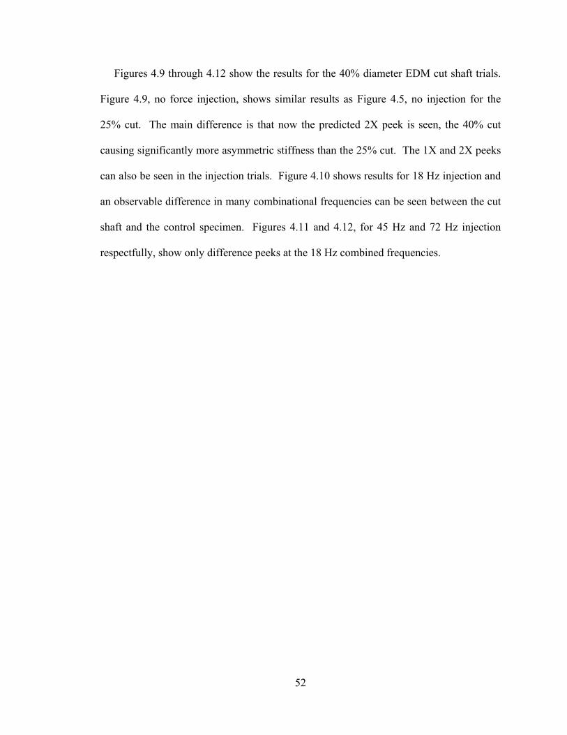
Figures 4.9 through 4.12 show the results for the 40% diameter EDM cut shaft trials.
Figure 4.9, no force injection, shows similar results as Figure 4.5, no injection for the
25% cut. The main difference is that now the predicted 2X peek is seen, the 40% cut
causing significantly more asymmetric stiffness than the 25% cut. The 1X and 2X peeks
can also be seen in the injection trials. Figure 4.10 shows results for 18 Hz injection and
an observable difference in many combinational frequencies can be seen between the cut
shaft and the control specimen. Figures 4.11 and 4.12, for 45 Hz and 72 Hz injection
respectfully, show only difference peeks at the 18 Hz combined frequencies.
52
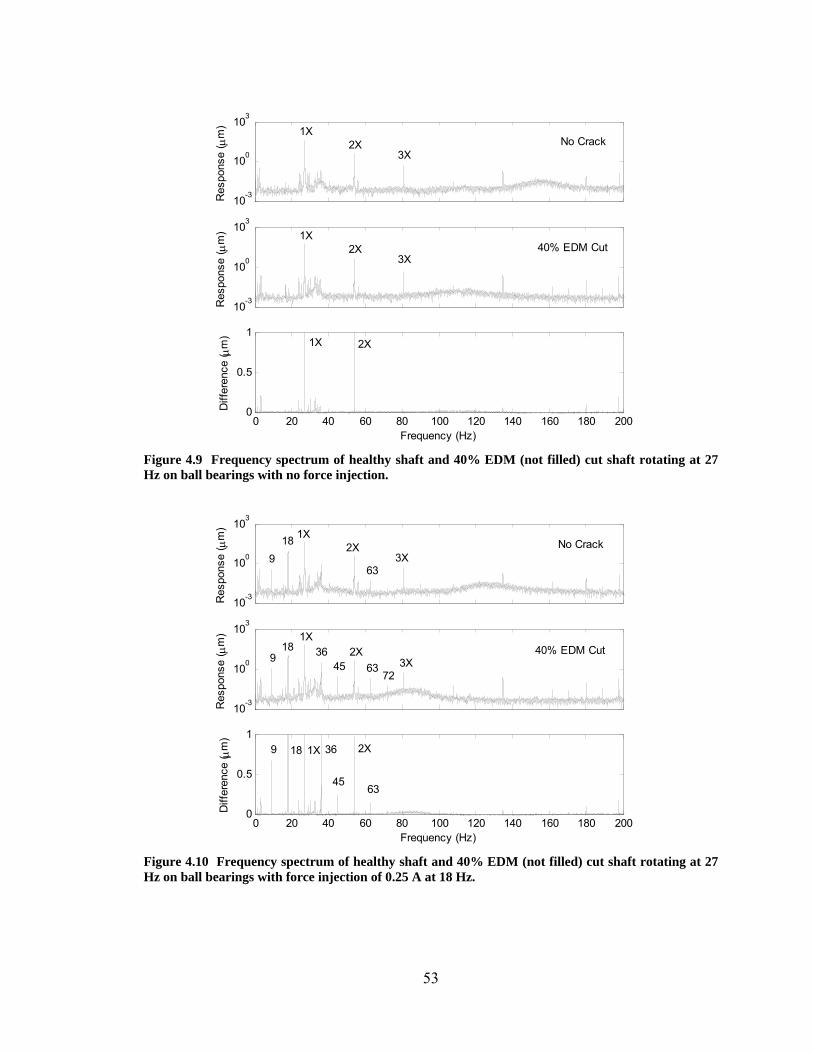
10-3
100
103
Res
pons
e ( μ
m)
10-3
100
103R
espo
nse
( μm
)
0 20 40 60 80 100 120 140 160 180 2000
0.5
1
Diff
eren
ce ( μ
m)
Frequency (Hz)
40% EDM Cut
No Crack 3X
2X 1X
1X 2X
3X
1X 2X
Figure 4.9 Frequency spectrum of healthy shaft and 40% EDM (not filled) cut shaft rotating at 27 Hz on ball bearings with no force injection.
10-3
100
103
Res
pons
e ( μ
m)
10-3
100
103
Res
pons
e ( μ
m)
0 20 40 60 80 100 120 140 160 180 2000
0.5
1
Diff
eren
ce ( μ
m)
Frequency (Hz)
1X 2X
3X No Crack
40% EDM Cut 9
181X
3645
2X 63
723X
918
63
9 18 1X 36
45
2X
63
Figure 4.10 Frequency spectrum of healthy shaft and 40% EDM (not filled) cut shaft rotating at 27 Hz on ball bearings with force injection of 0.25 A at 18 Hz.
53
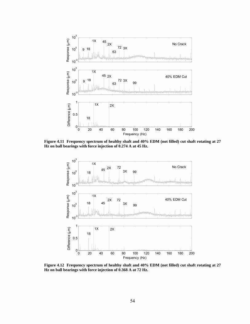
10-3
100
103
Res
pons
e ( μ
m)
10-3
100
103R
espo
nse
( μm
)
0 20 40 60 80 100 120 140 160 180 2000
0.5
1
Diff
eren
ce ( μ
m)
Frequency (Hz)
1X 2X
3X No Crack
40% EDM Cut 18
1X 45 2X
72 3X 9963
9
9 18
45
6372
18
1X 2X
Figure 4.11 Frequency spectrum of healthy shaft and 40% EDM (not filled) cut shaft rotating at 27 Hz on ball bearings with force injection of 0.274 A at 45 Hz.
10-3
100
103
Res
pons
e ( μ
m)
10-3
100
103
Res
pons
e ( μ
m)
0 20 40 60 80 100 120 140 160 180 2000
0.5
1
Diff
eren
ce ( μ
m)
Frequency (Hz)
1X 2X
3X No Crack
40% EDM Cut
991845
72
18
1X
452X 72
3X 99
181X 2X
Figure 4.12 Frequency spectrum of healthy shaft and 40% EDM (not filled) cut shaft rotating at 27 Hz on ball bearings with force injection of 0.368 A at 72 Hz.
54
Figures 4.13 through 4.16 show results for the shim filled 25% diameter EDM cut
shaft trials. For no injection, 1X difference and natural frequency shift can be seen
similar to the non shim filled case. For 18 Hz injection, Figure 4.14, a difference in the
combinational frequency at 45 Hz can be seen. Also, the difference in the 1X component
is much less. In Figures 4.15 and 4.16, injection at 45 Hz and 72 Hz respectfully, almost
no difference between the damaged and undamaged rotors can be seen at all.
55
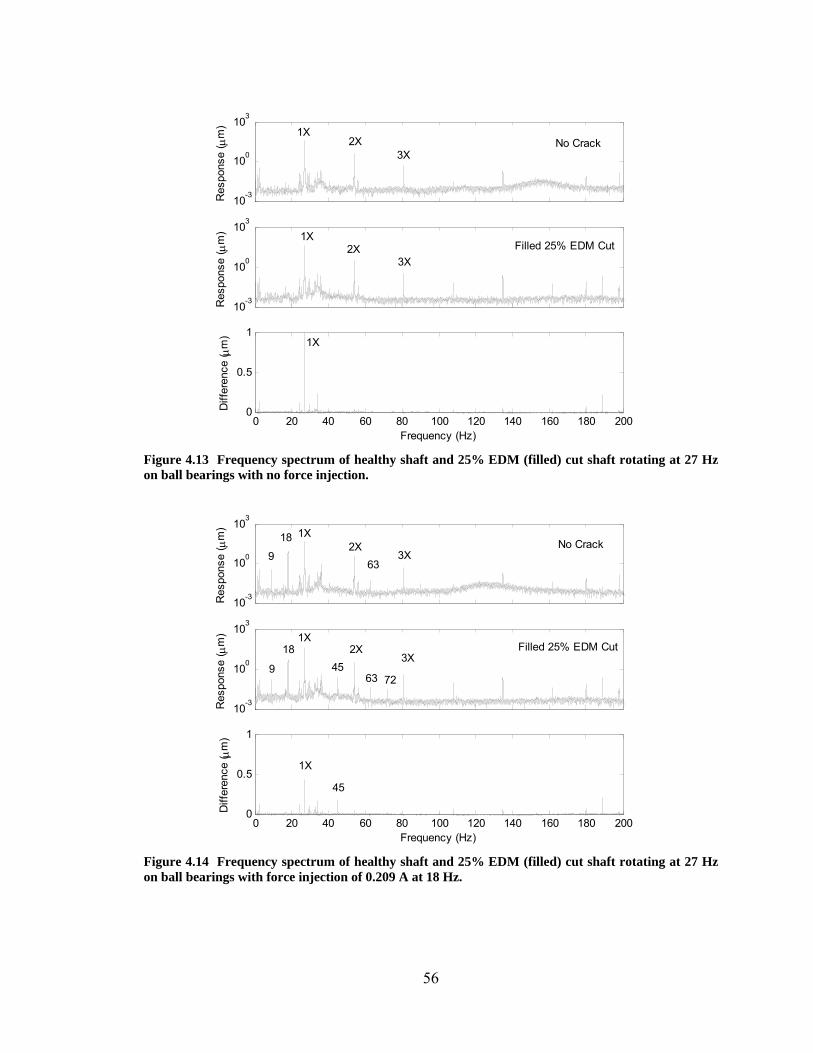
10-3
100
103
Res
pons
e ( μ
m)
10-3
100
103R
espo
nse
( μm
)
0 20 40 60 80 100 120 140 160 180 2000
0.5
1
Diff
eren
ce ( μ
m)
Frequency (Hz)
1X 2X
3X No Crack
Filled 25% EDM Cut1X
2X 3X
1X
Figure 4.13 Frequency spectrum of healthy shaft and 25% EDM (filled) cut shaft rotating at 27 Hz on ball bearings with no force injection.
10-3
100
103
Res
pons
e ( μ
m)
10-3
100
103
Res
pons
e ( μ
m)
0 20 40 60 80 100 120 140 160 180 2000
0.5
1
Diff
eren
ce ( μ
m)
Frequency (Hz)
1X 2X
3X No Crack
Filled 25% EDM Cut181X
452X
72
3X
18
45
639
963
1X
Figure 4.14 Frequency spectrum of healthy shaft and 25% EDM (filled) cut shaft rotating at 27 Hz on ball bearings with force injection of 0.209 A at 18 Hz.
56
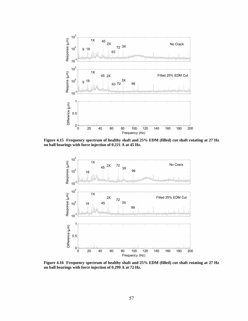
10-3
100
103
Res
pons
e ( μ
m)
10-3
100
103R
espo
ns ( μ
m)
0 20 40 60 80 100 120 140 160 180 2000
0.5
1
Diff
eren
ce ( μ
m)
Frequency (Hz)
1X 2X
3X No Crack
Filled 25% EDM Cut18
1X 45 2X
723X
999 63
7263
45
189
Figure 4.15 Frequency spectrum of healthy shaft and 25% EDM (filled) cut shaft rotating at 27 Hz on ball bearings with force injection of 0.221 A at 45 Hz.
10-3
100
103
Res
pons
e ( μ
m)
10-3
100
103
Res
pons
e ( μ
m)
0 20 40 60 80 100 120 140 160 180 2000
0.5
1
Diff
eren
ce ( μ
m)
Frequency (Hz)
1X 2X
3X No Crack
Filled 25% EDM Cut
1845 72
99
18
1X
452X 72
3X 99
Figure 4.16 Frequency spectrum of healthy shaft and 25% EDM (filled) cut shaft rotating at 27 Hz on ball bearings with force injection of 0.299 A at 72 Hz.
57
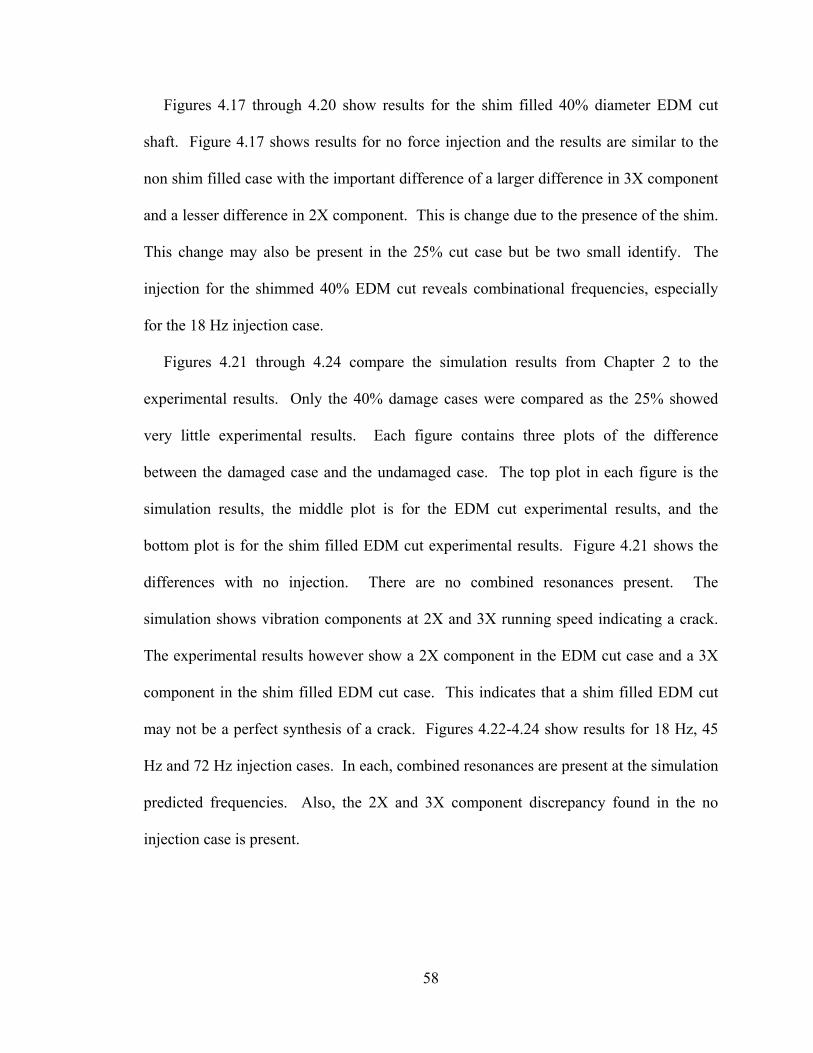
Figures 4.17 through 4.20 show results for the shim filled 40% diameter EDM cut
shaft. Figure 4.17 shows results for no force injection and the results are similar to the
non shim filled case with the important difference of a larger difference in 3X component
and a lesser difference in 2X component. This is change due to the presence of the shim.
This change may also be present in the 25% cut case but be two small identify. The
injection for the shimmed 40% EDM cut reveals combinational frequencies, especially
for the 18 Hz injection case.
Figures 4.21 through 4.24 compare the simulation results from Chapter 2 to the
experimental results. Only the 40% damage cases were compared as the 25% showed
very little experimental results. Each figure contains three plots of the difference
between the damaged case and the undamaged case. The top plot in each figure is the
simulation results, the middle plot is for the EDM cut experimental results, and the
bottom plot is for the shim filled EDM cut experimental results. Figure 4.21 shows the
differences with no injection. There are no combined resonances present. The
simulation shows vibration components at 2X and 3X running speed indicating a crack.
The experimental results however show a 2X component in the EDM cut case and a 3X
component in the shim filled EDM cut case. This indicates that a shim filled EDM cut
may not be a perfect synthesis of a crack. Figures 4.22-4.24 show results for 18 Hz, 45
Hz and 72 Hz injection cases. In each, combined resonances are present at the simulation
predicted frequencies. Also, the 2X and 3X component discrepancy found in the no
injection case is present.
58
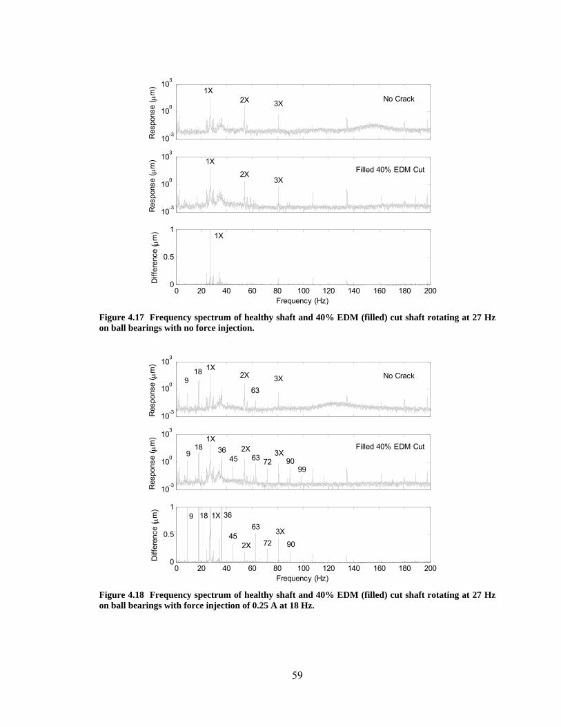
10-3
100
103
Res
pons
e ( μ
m)
10-3
100
103R
espo
nse
( μm
)
0 20 40 60 80 100 120 140 160 180 2000
0.5
1
Frequency (Hz)
Diff
eren
ce ( μ
m)
1X 2X 3X No Crack
Filled 40% EDM Cut1X
2X 3X
1X
Figure 4.17 Frequency spectrum of healthy shaft and 40% EDM (filled) cut shaft rotating at 27 Hz on ball bearings with no force injection.
10-3
100
103
Res
pons
e ( μ
m)
10-3
100
103
Res
pons
e ( μ
m)
0 20 40 60 80 100 120 140 160 180 2000
0.5
1
Frequency (Hz)
Diff
eren
ce ( μ
m)
1X 2X 3X No Crack
Filled 40% EDM Cut181X
452X
723X
99
3663 90
9
918
63
9 18 1X 36
452X
63
723X
90
Figure 4.18 Frequency spectrum of healthy shaft and 40% EDM (filled) cut shaft rotating at 27 Hz on ball bearings with force injection of 0.25 A at 18 Hz.
59
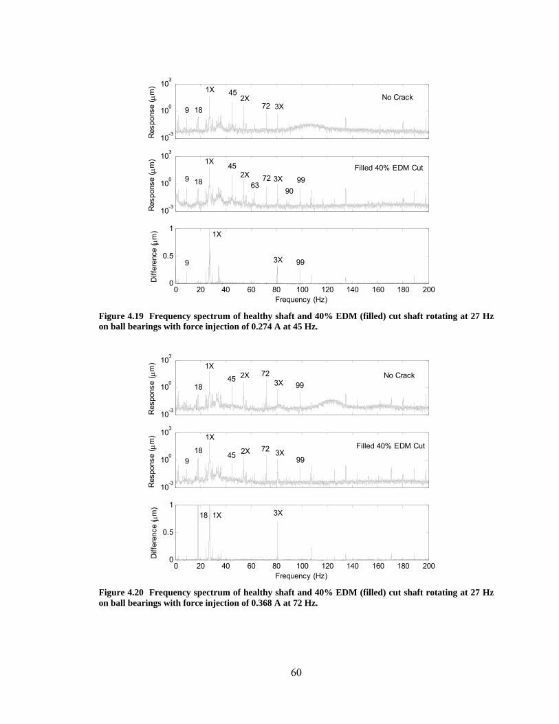
10-3
100
103
Res
pons
e ( μ
m)
10-3
100
103R
espo
nse
( μm
)
0 20 40 60 80 100 120 140 160 180 2000
0.5
1
Frequency (Hz)
Diff
eren
ce ( μ
m)
1X 2X
3X No Crack
Filled 40% EDM Cut9 18
1X 452X
6372 3X
9099
993X 9
9 18
45
72
1X
Figure 4.19 Frequency spectrum of healthy shaft and 40% EDM (filled) cut shaft rotating at 27 Hz on ball bearings with force injection of 0.274 A at 45 Hz.
10-3
100
103
Res
pons
e ( μ
m)
10-3
100
103
Res
pons
e ( μ
m)
0 20 40 60 80 100 120 140 160 180 2000
0.5
1
Frequency (Hz)
Diff
eren
ce ( μ
m)
1X 2X
3X No Crack
Filled 40% EDM Cut
1845
7299
18 45
1X
2X 72 3X 999
18 1X 3X
Figure 4.20 Frequency spectrum of healthy shaft and 40% EDM (filled) cut shaft rotating at 27 Hz on ball bearings with force injection of 0.368 A at 72 Hz.
60
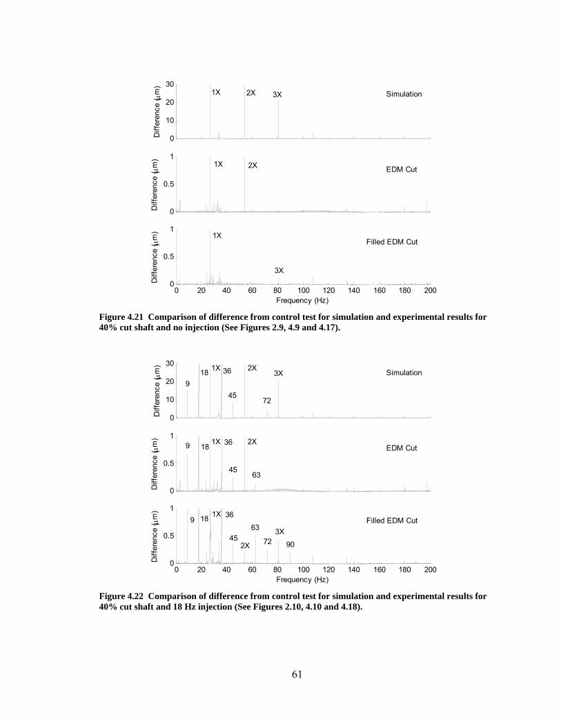
0
10
20
30
Diff
eren
ce ( μ
m)
0
0.5
1D
iffer
ence
( μm
)
0 20 40 60 80 100 120 140 160 180 2000
0.5
1
Frequency (Hz)
Diff
eren
ce ( μ
m)
Simulation
EDM Cut
Filled EDM Cut
1X 2X 3X
1X 2X
1X
3X
Figure 4.21 Comparison of difference from control test for simulation and experimental results for 40% cut shaft and no injection (See Figures 2.9, 4.9 and 4.17).
0
10
20
30
Diff
eren
ce ( μ
m)
0
0.5
1
Diff
eren
ce ( μ
m)
0 20 40 60 80 100 120 140 160 180 2000
0.5
1
Frequency (Hz)
Diff
eren
ce ( μ
m)
Simulation
EDM Cut
Filled EDM Cut
1X 2X 3X
9 18
45 72
9 18 1X
45
2X
9 18 1X
45 2X 72
3X 63
63
36
36
36
90
Figure 4.22 Comparison of difference from control test for simulation and experimental results for 40% cut shaft and 18 Hz injection (See Figures 2.10, 4.10 and 4.18).
61
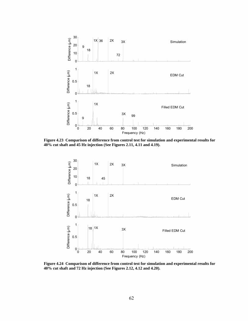
0
10
20
30
Diff
eren
ce ( μ
m)
0
0.5
1D
iffer
ence
( μm
)
0 20 40 60 80 100 120 140 160 180 2000
0.5
1
Frequency (Hz)
Diff
eren
ce ( μ
m)
Simulation
EDM Cut
Filled EDM Cut
9 18
1X 2X 3X
72
36
18
1X 2X
9
1X
3X 99
Figure 4.23 Comparison of difference from control test for simulation and experimental results for 40% cut shaft and 45 Hz injection (See Figures 2.11, 4.11 and 4.19).
0
10
20
30
Diff
eren
ce ( μ
m)
0
0.5
1
Diff
eren
ce ( μ
m)
0 20 40 60 80 100 120 140 160 180 2000
0.5
1
Frequency (Hz)
Diff
eren
ce ( μ
m)
Simulation
EDM Cut
Filled EDM Cut
1X 2X 3X
18 1X 2X
18 1X 3X
18 45
Figure 4.24 Comparison of difference from control test for simulation and experimental results for 40% cut shaft and 72 Hz injection (See Figures 2.12, 4.12 and 4.20).
62
4.3 Magnetically Levitated Rotor
4.3.1 Controller Design and Implementation
A MatLab Simulink model is used to design and examine the behavior and verify the
stability of the magnetic levitation controller before the levitated trials are conducted
experimentally. Figure 4.25 shows the Simulink model of the overall closed loop
feedback control system. A state-space representation of the rotor is generated using the
program MODAL version 1.5 which is part of the software package generated by the
University of Virginia Rotating Machinery and Controls (ROMAC) Laboratory. This
serves as the plant in the control loop and has six force inputs and eight position outputs.
Each magnetic bearing is controlled independently in SISO fashion. Figure 4.26 shows
the model for each magnetic bearing axis. The linear approximations discussed in section
3.2.1 are used.
An impulse input at 1 sec. was used to test the controller’s stability. Figures 4.27 and
4.28 show the impulse response. Figure 4.27 is the response of a levitated non-rotating
rotor and Figure 4.28 shows the response of a rotor spinning at 27 Hz with corresponding
unbalance force at the disk. An unbalance of 0.001 kg-m is used.
63
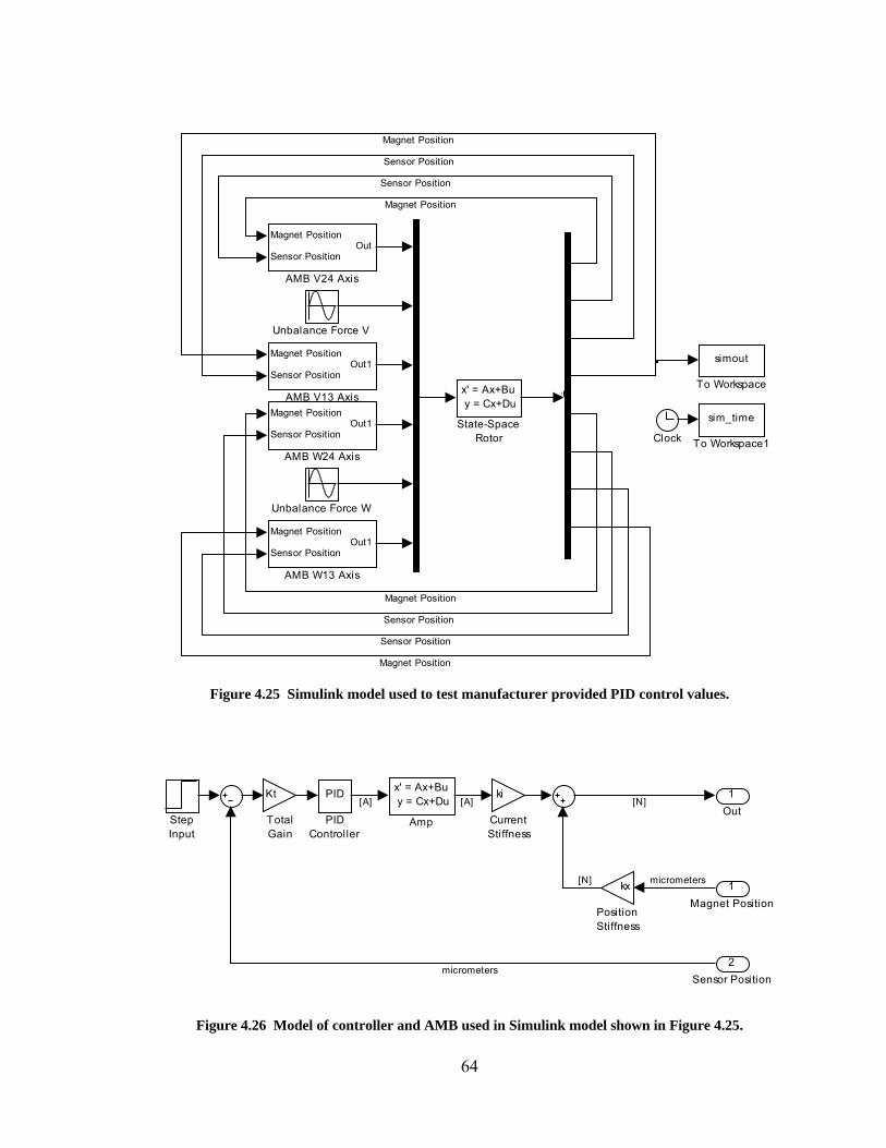
Unbalance Force W
Unbalance Force V
sim_time
To Workspace1
simout
To Workspacex' = Ax+Bu y = Cx+Du
State-SpaceRotor
em
Clock
Magnet Position
Sensor PositionOut1
AMB W24 Axis
Magnet Position
Sensor PositionOut1
AMB W13 Axis
Magnet Position
Sensor PositionOut
AMB V24 Axis
Magnet Position
Sensor PositionOut1
AMB V13 Axis
Sensor Position
Sensor Position
Magnet Position
Magnet Position
Sensor Position
Sensor Position
Magnet Position
Magnet Position
Figure 4.25 Simulink model used to test manufacturer provided PID control values.
1Out
Kt
TotalGain
StepInput
kx
PositionStiffness
PID
PIDController
ki
CurrentStiffness
x' = Ax+Bu y = Cx+Du
Amp
2Sensor Position
1Magnet Position
[N]
micrometers
micrometers
[N][A][A]
Figure 4.26 Model of controller and AMB used in Simulink model shown in Figure 4.25.
64
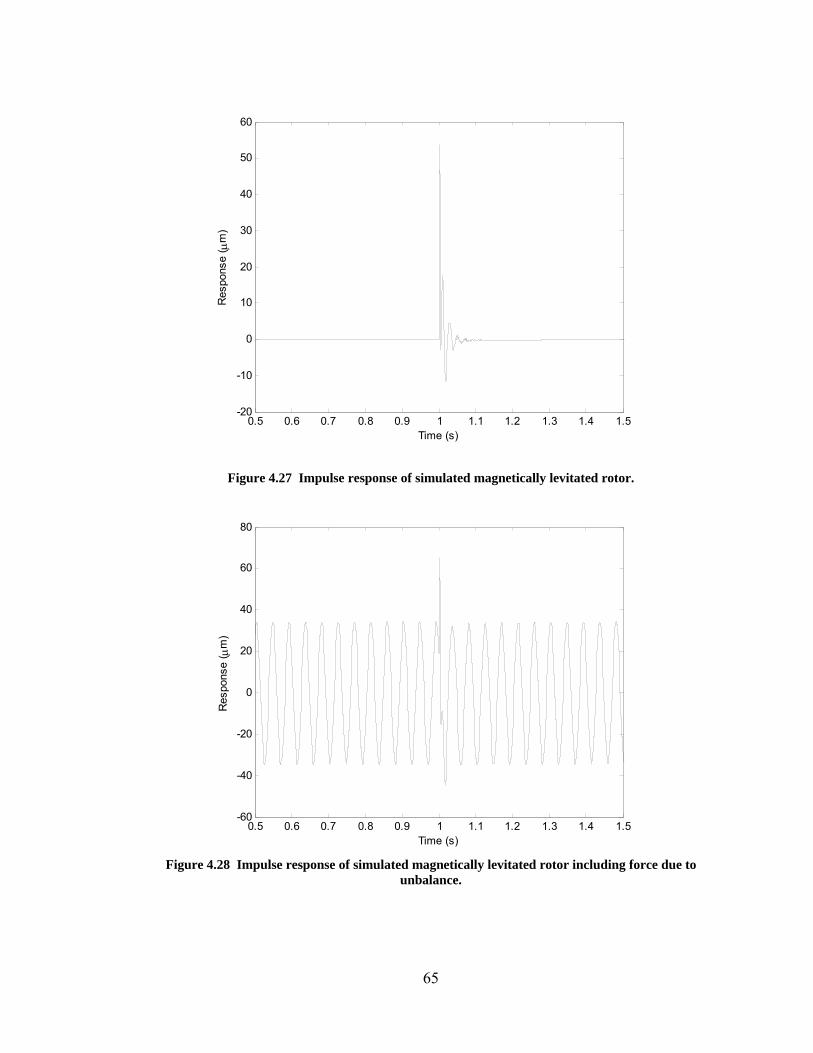
0.5 0.6 0.7 0.8 0.9 1 1.1 1.2 1.3 1.4 1.5-20
-10
0
10
20
30
40
50
60
Time (s)
Res
pons
e ( μ
m)
Figure 4.27 Impulse response of simulated magnetically levitated rotor.
0.5 0.6 0.7 0.8 0.9 1 1.1 1.2 1.3 1.4 1.5-60
-40
-20
0
20
40
60
80
Time (s)
Res
pons
e ( μ
m)
Figure 4.28 Impulse response of simulated magnetically levitated rotor including force due to
unbalance.
65
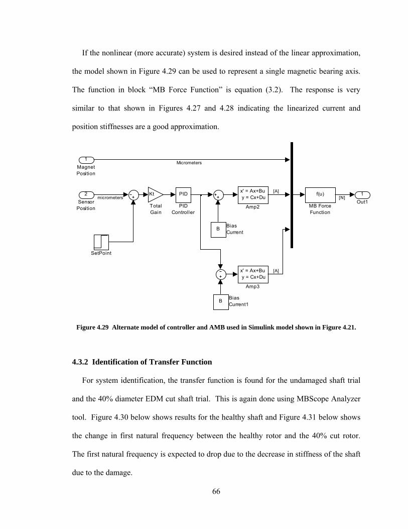
If the nonlinear (more accurate) system is desired instead of the linear approximation,
the model shown in Figure 4.29 can be used to represent a single magnetic bearing axis.
The function in block “MB Force Function” is equation (3.2). The response is very
similar to that shown in Figures 4.27 and 4.28 indicating the linearized current and
position stiffnesses are a good approximation.
1Out1
Kt
TotalGain
SetPoint
PID
PIDController
f(u)
MB ForceFunction
B BiasCurrent1
B BiasCurrent
x' = Ax+Bu y = Cx+Du
Amp3
x' = Ax+Bu y = Cx+Du
Amp2
2Sensor
Position
1MagnetPosition
micrometers
Micrometers
[A]
[A]
[N]
Figure 4.29 Alternate model of controller and AMB used in Simulink model shown in Figure 4.21.
4.3.2 Identification of Transfer Function
For system identification, the transfer function is found for the undamaged shaft trial
and the 40% diameter EDM cut shaft trial. This is again done using MBScope Analyzer
tool. Figure 4.30 below shows results for the healthy shaft and Figure 4.31 below shows
the change in first natural frequency between the healthy rotor and the 40% cut rotor.
The first natural frequency is expected to drop due to the decrease in stiffness of the shaft
due to the damage.
66
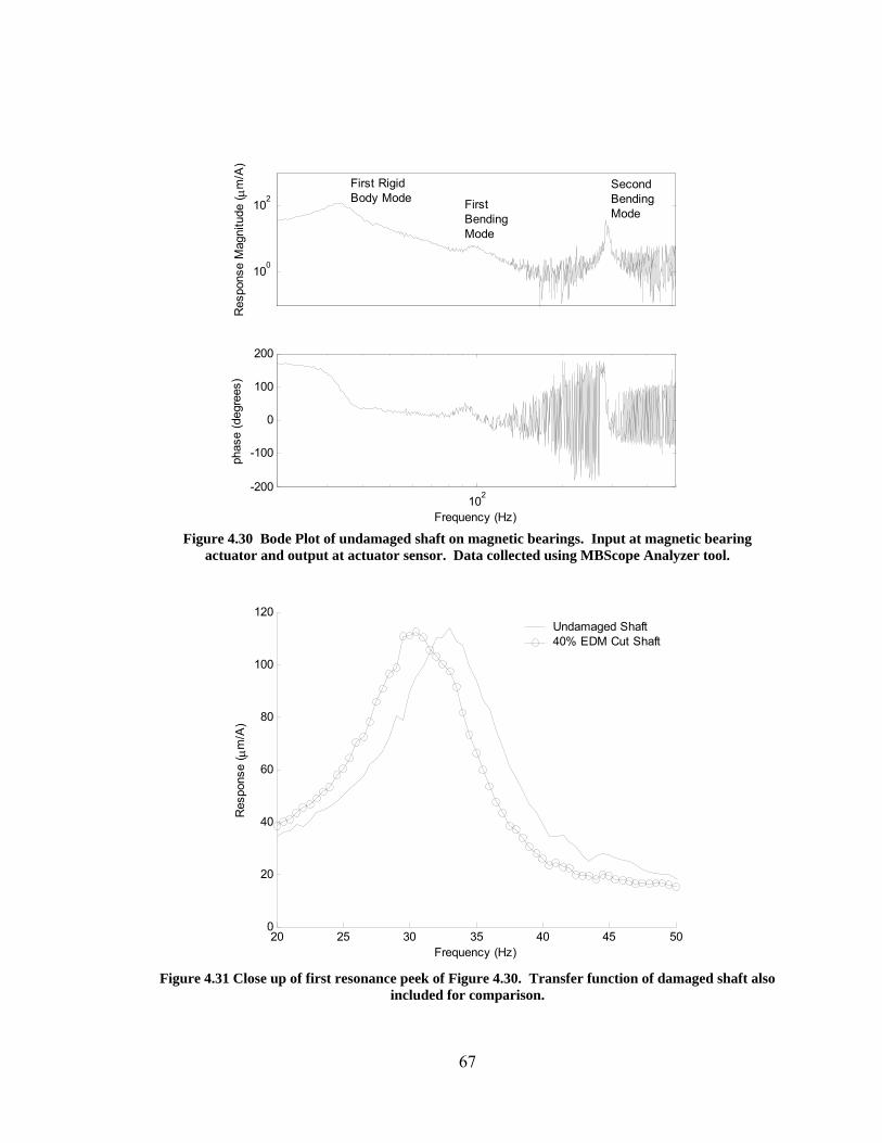
100
102
Res
pons
e M
agni
tude
( μm
/A)
102-200
-100
0
100
200
Frequency (Hz)
phas
e (d
egre
es)
First RigidBody Mode
SecondBendingMode
FirstBendingMode
Figure 4.30 Bode Plot of undamaged shaft on magnetic bearings. Input at magnetic bearing
actuator and output at actuator sensor. Data collected using MBScope Analyzer tool.
20 25 30 35 40 45 500
20
40
60
80
100
120
Frequency (Hz)
Res
pons
e ( μ
m/A
)
Undamaged Shaft40% EDM Cut Shaft
Figure 4.31 Close up of first resonance peek of Figure 4.30. Transfer function of damaged shaft also
included for comparison.
67
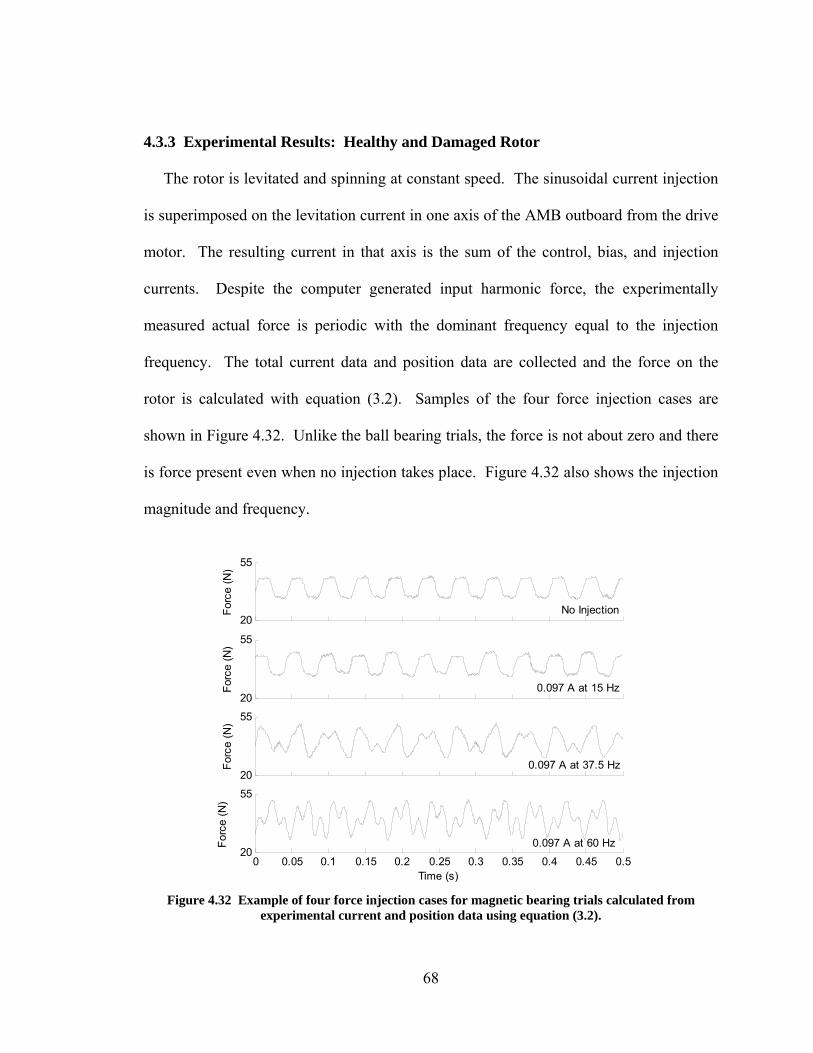
4.3.3 Experimental Results: Healthy and Damaged Rotor
The rotor is levitated and spinning at constant speed. The sinusoidal current injection
is superimposed on the levitation current in one axis of the AMB outboard from the drive
motor. The resulting current in that axis is the sum of the control, bias, and injection
currents. Despite the computer generated input harmonic force, the experimentally
measured actual force is periodic with the dominant frequency equal to the injection
frequency. The total current data and position data are collected and the force on the
rotor is calculated with equation (3.2). Samples of the four force injection cases are
shown in Figure 4.32. Unlike the ball bearing trials, the force is not about zero and there
is force present even when no injection takes place. Figure 4.32 also shows the injection
magnitude and frequency.
20
55
Forc
e (N
)
20
55
Forc
e (N
)
20
55
Forc
e (N
)
0 0.05 0.1 0.15 0.2 0.25 0.3 0.35 0.4 0.45 0.520
55
Time (s)
Forc
e (N
)
No Injection
0.097 A at 15 Hz
0.097 A at 37.5 Hz
0.097 A at 60 Hz
Figure 4.32 Example of four force injection cases for magnetic bearing trials calculated from
experimental current and position data using equation (3.2).
68
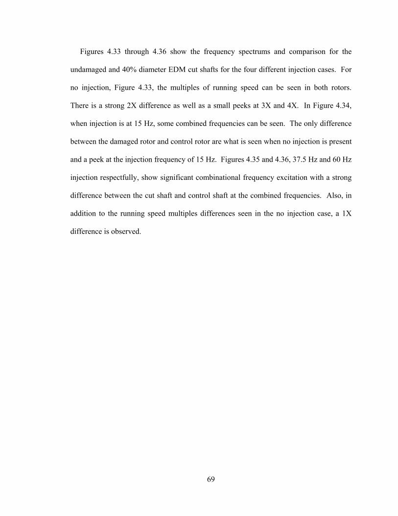
Figures 4.33 through 4.36 show the frequency spectrums and comparison for the
undamaged and 40% diameter EDM cut shafts for the four different injection cases. For
no injection, Figure 4.33, the multiples of running speed can be seen in both rotors.
There is a strong 2X difference as well as a small peeks at 3X and 4X. In Figure 4.34,
when injection is at 15 Hz, some combined frequencies can be seen. The only difference
between the damaged rotor and control rotor are what is seen when no injection is present
and a peek at the injection frequency of 15 Hz. Figures 4.35 and 4.36, 37.5 Hz and 60 Hz
injection respectfully, show significant combinational frequency excitation with a strong
difference between the cut shaft and control shaft at the combined frequencies. Also, in
addition to the running speed multiples differences seen in the no injection case, a 1X
difference is observed.
69
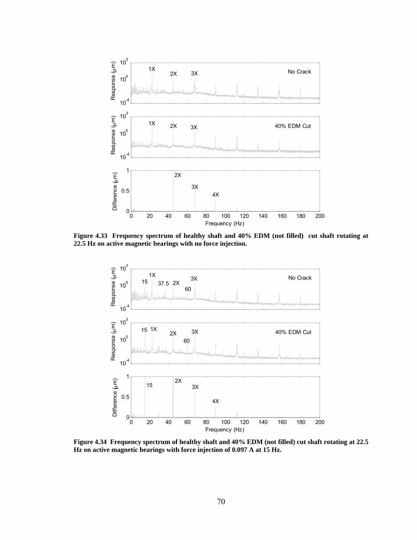
10-4
100
103
Res
pons
e ( μ
m)
10-4
100
103R
espo
nse
( μm
)
0 20 40 60 80 100 120 140 160 180 2000
0.5
1
Frequency (Hz)
Diff
eren
ce ( μ
m)
1X 2X 3X No Crack
40% EDM Cut 3X 2X 1X
4X 3X
2X
Figure 4.33 Frequency spectrum of healthy shaft and 40% EDM (not filled) cut shaft rotating at 22.5 Hz on active magnetic bearings with no force injection.
10-4
100
103
Res
pons
e ( μ
m)
10-4
100
103
Res
pons
e ( μ
m)
0 20 40 60 80 100 120 140 160 180 2000
0.5
1
Frequency (Hz)
Diff
eren
ce ( μ
m)
1X 2X
3X No Crack
40% EDM Cut
37.515
15 1X 2X 3X
152X
3X
4X
60
60
Figure 4.34 Frequency spectrum of healthy shaft and 40% EDM (not filled) cut shaft rotating at 22.5 Hz on active magnetic bearings with force injection of 0.097 A at 15 Hz.
70
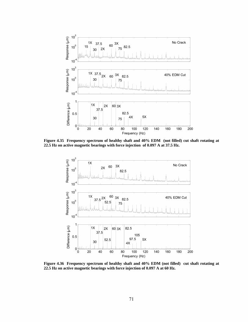
10-4
100
103
Res
pons
e ( μ
m)
10-4
100
103R
espo
nse
( μm
)
0 20 40 60 80 100 120 140 160 180 2000
0.5
1
Frequency (Hz)
Diff
eren
ce ( μ
m)
1X
2X 3X No Crack
40% EDM Cut
1537.5 60
75 82.5
1X 37.52X 60 3X
7582.5
82.5
75
3X 602X 37.5
1X
4X 5X
30
30
30
Figure 4.35 Frequency spectrum of healthy shaft and 40% EDM (not filled) cut shaft rotating at 22.5 Hz on active magnetic bearings with force injection of 0.097 A at 37.5 Hz.
10-4
100
103
Res
pons
e ( μ
m)
10-4
100
103
Res
pons
e ( μ
m)
0 20 40 60 80 100 120 140 160 180 2000
0.5
1
Frequency (Hz)
Diff
eren
ce ( μ
m)
1X 2X 3X No Crack
40% EDM Cut 1X 37.5 2X 60 3X
7582.5
52.5
1X 37.5
2X 60 3X 82.5
4X 5X
52.5
30
6082.5
97.5105
Figure 4.36 Frequency spectrum of healthy shaft and 40% EDM (not filled) cut shaft rotating at 22.5 Hz on active magnetic bearings with force injection of 0.097 A at 60 Hz.
71
CHAPTER V
CONCLUSIONS
5.1 Contributions
Condition monitoring of machinery is a vast growing industry. In the last two decades
a variety of approaches have been proposed to try to make use of the changes in the
dynamics of a rotor to identify and possibly locate a crack (and other faults) in the rotor
at an early stage in their development.
In this thesis, the modeling of the cracked Jeffcott rotor subjected to residual
unbalance, gravity force and externally applied harmonic force excitation has been
presented in attempt to use the changes in the dynamics of the rotor to identify the
presence of a crack. The generated simulation results demonstrate that the use of an
active magnetic bearing (AMB) to excite the rotor with a harmonic force at a carefully
selected frequency produces components in the system response at many frequencies
72
which are combinations of the rotor speed, the AMB excitation frequency and the system
natural frequency which are not present in an un-cracked rotor.
In order to verify the predicted results an extensive experimental matrix has been
followed using a dedicated crack detection experimental facility. The conducted
experimental study involved external excitation applied between the supporting bearings
and at the supporting bearing. In the first case the rotor was supported on ball bearings
while in the second case the rotor was magnetically levitated. The PID controller, of
which, was successfully developed for magnetic rotor levitation. A check of the stability
and robustness of the controller has been carried out using MatLab Simulink.
This work contributes to the art of online health monitoring by experimentally
confirming the presence of combinational frequencies in a cracked rotor’s vibration. In
most of the tested operating conditions, the measured rotor response for the cracked rotor
exhibited the same frequency components as predicted in the simulation. Those
components, being combination frequencies of three main, different system frequencies
present in a system, have a potential to be used to detect cracks in the rotor. It is also a
noteworthy contribution that the combination frequencies were also found in the response
of the magnetically levitated cracked rotor with the excitation applied at the supporting
bearing.
5.2 Further Research Directions
Further research is needed to make the presented approach a practical condition
monitoring technique. Although AMB technology seems to lend itself naturally to the
role of calibrated actuator or force transducer, accuracy limits are significant. Also, a
73
more robust technique is needed to determine the presence, location and severity of a
crack from the combination frequencies in the response. Furthermore the effect of adding
an extra force to the system might encourage a faster crack growth, which is obviously a
disadvantage. This method can be applied to magnetically levitated systems with no
additional hardware, but for traditionally supported rotors, an additional component
would have to be provided.
Areas of research needed to develop practical application of this crack detection
method include the following. This simulation and experiment should be repeated for a
wider range of parameters including but not limited to crack location and depth, rotor
dimensions, operating speeds, and injection frequencies. This method should be tested
using proper safety precautions on a rotor with a true crack. This method should be
tested on an actual operable machine to serve as a case study in finding optimum force
injection values and frequencies.
74
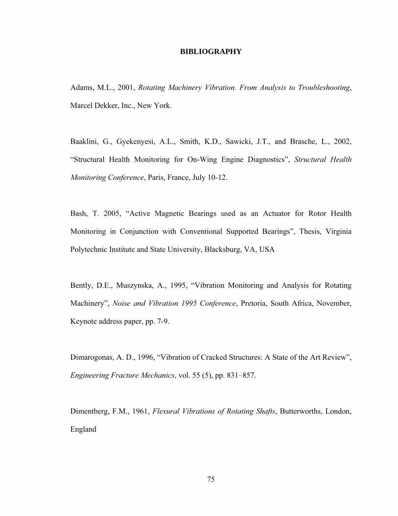
BIBLIOGRAPHY
Adams, M.L., 2001, Rotating Machinery Vibration. From Analysis to Troubleshooting,
Marcel Dekker, Inc., New York.
Baaklini, G., Gyekenyesi, A.L., Smith, K.D., Sawicki, J.T., and Brasche, L., 2002,
“Structural Health Monitoring for On-Wing Engine Diagnostics”, Structural Health
Monitoring Conference, Paris, France, July 10-12.
Bash, T. 2005, “Active Magnetic Bearings used as an Actuator for Rotor Health
Monitoring in Conjunction with Conventional Supported Bearings”, Thesis, Virginia
Polytechnic Institute and State University, Blacksburg, VA, USA
Bently, D.E., Muszynska, A., 1995, “Vibration Monitoring and Analysis for Rotating
Machinery”, Noise and Vibration 1995 Conference, Pretoria, South Africa, November,
Keynote address paper, pp. 7-9.
Dimarogonas, A. D., 1996, “Vibration of Cracked Structures: A State of the Art Review”,
Engineering Fracture Mechanics, vol. 55 (5), pp. 831–857.
Dimentberg, F.M., 1961, Flexural Vibrations of Rotating Shafts, Butterworths, London,
England
75
Doebling, S.W., Farrar, C.R., Prime, M.B., and Shevitz, D.W., 1996, Los Alamos
National Laboratory Report LA-13070-MS.
Dimarogonas, A.D., 1973, “Newkirk Effect, Thermally Induced Dynamic Instability of
High Speed Rotors”, International Gas Turbine Conference, Washington, D.C., ASME
Paper No. 73-GT-26.
Dimarogonas, A.D., 1983, “Analytical Methods in Rotor Dynamics”, Applied Science
Publishers, London.
Earnshaw, S., 1842, On the Nature of the Molecular Forces Which Regulate the
Constitution of the Lumiferous Ether, Trans. Camb. Phil. Soc., 7, Part I: 97–112.
Ehrich, F., ed., 1992, Handbook of Rotordynamics, McGraw Hill Inc., New York.
Evans, D.J., Pusey, H.C., 2002, “Shock and Vibration Standards”, Harris’ Shock and
Vibration Handbook, Fifth Edition, McGraw-Hill, New York.
Gasch, R., 1976, “Dynamic Behaviour of a Simple Rotor with a Cross Sectional Crack”,
International Conference on Vibrations in Rotating Machinery, IMechE , Paper C178/76,
pp. 123-128.
76
Gasch, R.A., 1993, “Survey of the Dynamic Behavior of a Simple Rotating Shaft with a
Transverse Crack”, Journal of Sound and Vibration, Vol. 160, pp. 313-332.
Gasch, R. 2008 “Dynamic Behaviour of the Laval Rotor with a Transverse Crack”,
Mechanical Systems and Signal Processing, Vol. 22, pp. 790-804.
Gyekenyesi, A.L., Sawicki, J.T., and Baaklini, G., 2002, “Application of Vibration
Monitoring Techniques for Damage Detection in Rotating Disks”, The 9th International
Symposium on Transport Phenomena and Dynamics of Rotating Machinery, ISROMAC-
9, Honolulu, Hawaii, 10-14 February.
Ishida, Y., Tsuyoshi, I. 2006, “Detection of a Rotor Crack Using a Harmonic Excitation
and Nonlinear Vibration Analysis”, Journal of Vibration and Acoustics, Vol. 128, pp.
741-749.
Iwatsubo, T., Arii, S. and Oks, A., 1992, “Detection of a transverse crack in a rotor shaft
by adding external force”, Proc. IMechE Vibrations in Rotating Machinery, Vol.
C432/093, pp. 275-282 .
Kasarda, M., Quinn, D.D., Bash, T., Mani, G., Inman, D., Kirk, R.G., Sawicki, J.T.,
2005, “Magnetic Bearings for Non-destructive Health Monitoring of Rotating Machinery
Supported in Conventional Bearings”, Key Engineering Materials, Vols. 293-294, pp.
383-390.
77
Kellenberger, W., 1980, “Spiral Vibrations Due to Seal Rings in Turbogenerators.
Thermally Induced Interaction between Rotor and Stator”, ASME Journal of Mechanical
Design, Vol. 102, pp. 177-184.
Mani, G., Quinn, D., Kasarda, M. 2006, “Active Health Monitoring in a Rotating
Cracked Shaft Using Active Magneitc Bearings as Force Actuators”, Journal of Sound
and Vibration, Vol. 294, pp. 454-465.
Mani, G., Quinn, D.D., Kasarda, M.E.F., Inman, D.J. and Kirk, R.G., 2005, “Health
Monitoring of Rotating Machinery Through External Forcing”, Proceedings of
ISCORMA-3, Cleveland, Ohio, USA.
Mayes, I.W. and Davies, W.G.R., 1980, “A Method of Calculating the Vibrational
Behaviour of Coupled Rotating Shafts Containing a Transverse Crack”, International
Conference on Vibrations in Rotating Machinery, Paper C254/80, IMechE, pp. 17-27.
Mayes, I. W. and Davies, W. G. R., 1984, “Analysis of the Response of a Multi-Rotor-
Bearing System Containing a Transverse Crack in a Rotor”, ASME Journal of Vibration,
Acoustics, Stress, and Reliability in Design, Vol. 106, pp. 139-145.
Mitchell, J.S., 1993, Introduction to Machinery Analysis and Monitoring, Second Edition,
Penn Well Books, Tulsa, OK.
78
Muszynska, A., 1993, “Thermal Rub Effect in Rotating Machines,” ORBIT, Vol. 14, No.
1, pp. 8-13.
Morton, P.G., 1975, “The Derivation of Bearing Characteristics by Means of Transient
Excitation Applied Directly to a Rotating Shaft”, UTAM Symposium, Dynamics of
Rotors, pp. 350-370.
Muszynska, A., 1995, “Vibrational Diagnostics of Rotating Machinery Malfunctions”,
International Journal of Rotating Machinery, vol. 1, no. 3-4, pp. 237-266..
Newkirk, B.L., 1926, “Shaft Rubbing. Relative Freedom of Rotor Shafts from
Sensitiveness to Rubbing Contact When Running Above Their Critical Speeds”,
Mechanical Engineering, vol. 48, No. 8, pp. 830-832.
Nordmann, R., Aenis, M., 2004, “Fault Diagnosis in a Centrifugal Pump Using Active
Magnetic Bearings”, International Journal of Rotating Machinery, Vol. 10(3), pp. 183-
191.
Nordmann, R. and Schollhorn, K., 1984, “Identification of Modal Parameters of an
Elastic Rotor with Oil Film Bearings”, ASME Journal of Vibration, Acoustics, Stress, and
Reliability in Design, Vol. 106.
79
Penny, J., Friswell, M., Zhou, C., 2006, “Condition Monitoring of Rotating Machinery
Using Active Magnetic Bearings”, Proceedings of ISMA 2006, pp. 3497-3506.
Plonus, M. A., 1978, “Applied Electromagnetics”, McGraw-Hill, New York, pp. 410,
414-416.
Pusey, H.C., 1999, “An Assessment of Turbomachinery Condition Monitoring and
Failure Prognosis Technology”, Proceedings of 17th International Modal Analysis
Conference, Kissimmee, FL, February, pp. 1310-1316.
Quinn, D., Mani, G., Kasarda, M., Bash, T., Inman, J., Kirk, G., 2005, “Damage
Detection of a Rotating Cracked Shaft Using an Active Magnetic Bearing as a Force
Actuator – Analysis and Experimental Verification”, IEEE/ASME Transactions on
Mechatronics, Vol. 10, No. 6, pp. 640-647.
Rieger, N.F., McCloskey, T.H., and Dewey, R.P., 1990, “The High Cost of Failure of
Rotating Equipment”, Proceedings of 44th Meeting of the Mechanical Failure Prevention
Group, Vibration Institute.
Sawicki, J.T., 2002, “Some Advances in Diagnostics of Rotating Machinery
Malfunctions”, Proceedings of the Int. Symposium on Machine Condition Monitoring and
Diagnosis, The University of Tokyo, Tokyo, pp. 138-143.
80
Sawicki, J., Friswell, M., Pesch, A., Wroblewski, A., 2008, “Condition Monitoring of
Rotor Using Active Magnetic Actuator”, Proceedings of ASME Turbo Expo 2008: Power
for Land Sea and Air, Berlin, Germany.
Sawicki, J.T., Genta, G., 2001, “Modal Uncoupling of Damped Gyroscopic Systems”,
Journal of Sound and Vibration, vol. 244(3), pp. 431-451.
Sawicki, J.T., Montilla-Bravo, A., and Gosiewski, Z., 2003, “Thermo-Mechanical
Behavior of Rotor with Rubbing”, International Journal of Rotating Machinery. Vol.
9(1), pp. 41-47.
Sawicki, J.T., Padovan, J., and Al-Khatib, R., 1999, “The Dynamics of Rotor with
Rubbing”, International Journal of Rotating Machinery, Vol. 5, no. 4, pp. 295-304.
Taylor, H.D., 1924, “Rubbing Shafts Above and Below the Critical Speed”, General
Electric Review, Vol. 27.
Tonnesen, J. and Lund, J., 1988, “Experimental techniques for rotordynamic analysis”,
CISM Course No. 297, Rotordynamics 2.
Wauer, J., 1990, “On the Dynamics of Cracked Rotors: A Literature Survey”, Trans.
ASME, J. Appl. Mech., Vol. 43, pp. 13-17.
81

APPENDICES
82
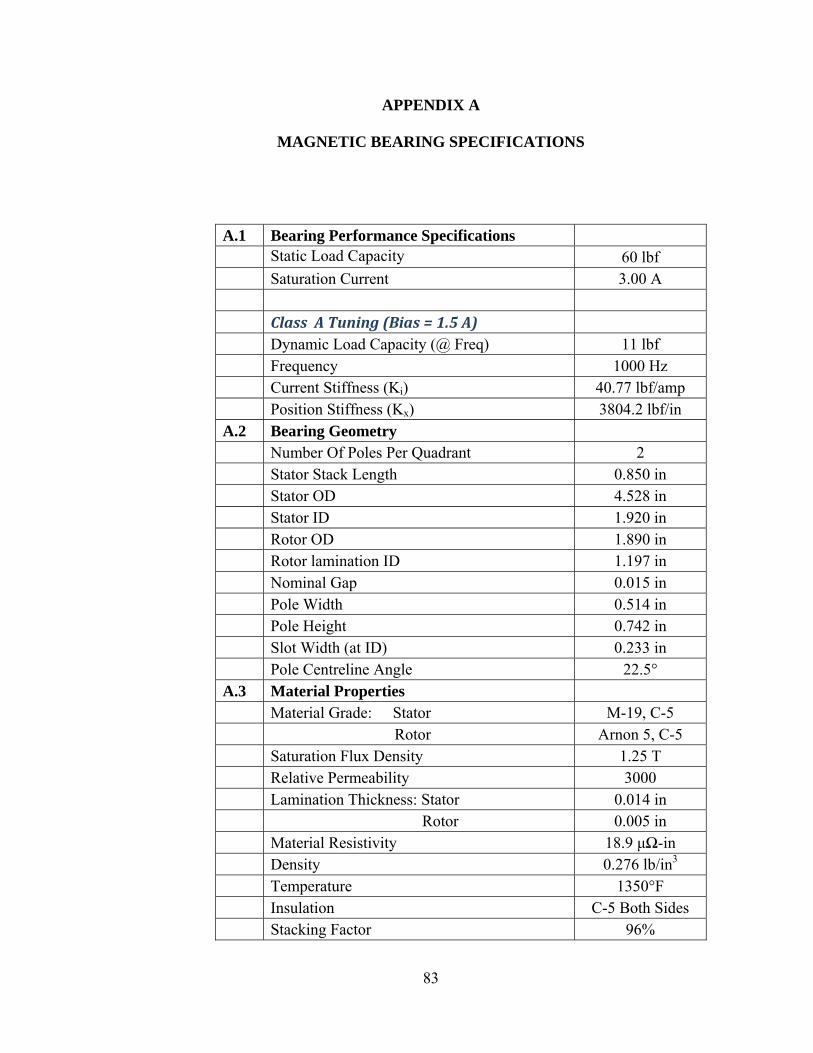
APPENDIX A
MAGNETIC BEARING SPECIFICATIONS
A.1 Bearing Performance Specifications Static Load Capacity 60 lbf Saturation Current 3.00 A Class A Tuning (Bias = 1.5 A) Dynamic Load Capacity (@ Freq) 11 lbf Frequency 1000 Hz Current Stiffness (Ki) 40.77 lbf/amp Position Stiffness (Kx) 3804.2 lbf/in A.2 Bearing Geometry Number Of Poles Per Quadrant 2 Stator Stack Length 0.850 in Stator OD 4.528 in Stator ID 1.920 in Rotor OD 1.890 in Rotor lamination ID 1.197 in Nominal Gap 0.015 in Pole Width 0.514 in Pole Height 0.742 in Slot Width (at ID) 0.233 in Pole Centreline Angle 22.5° A.3 Material Properties Material Grade: Stator M-19, C-5 Rotor Arnon 5, C-5 Saturation Flux Density 1.25 T Relative Permeability 3000 Lamination Thickness: Stator 0.014 in Rotor 0.005 in Material Resistivity 18.9 μΩ-in Density 0.276 lb/in3 Temperature 1350°F Insulation C-5 Both Sides Stacking Factor 96%
83
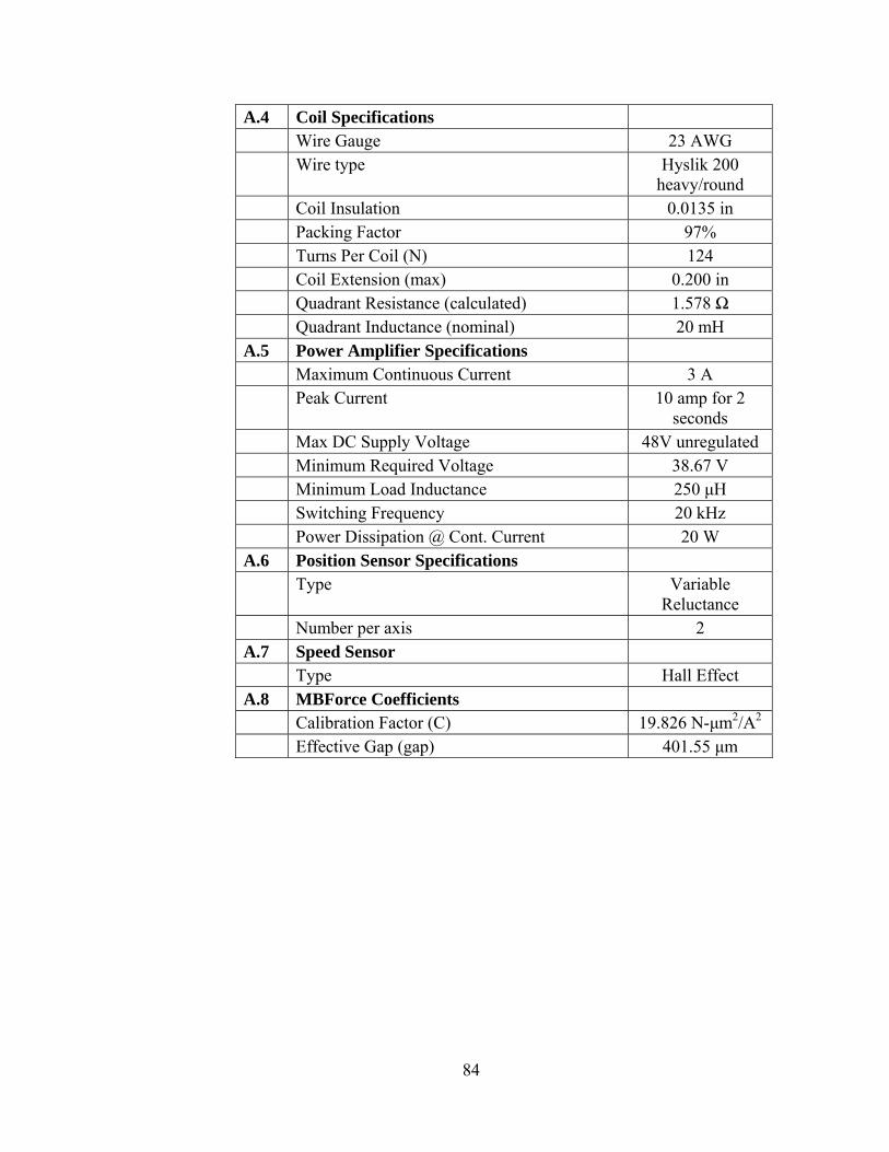
A.4 Coil Specifications Wire Gauge 23 AWG Wire type Hyslik 200
heavy/round Coil Insulation 0.0135 in Packing Factor 97% Turns Per Coil (N) 124 Coil Extension (max) 0.200 in Quadrant Resistance (calculated) 1.578 Ω Quadrant Inductance (nominal) 20 mH A.5 Power Amplifier Specifications Maximum Continuous Current 3 A Peak Current 10 amp for 2
seconds Max DC Supply Voltage 48V unregulated Minimum Required Voltage 38.67 V Minimum Load Inductance 250 μH Switching Frequency 20 kHz Power Dissipation @ Cont. Current 20 W A.6 Position Sensor Specifications Type Variable
Reluctance Number per axis 2 A.7 Speed Sensor Type Hall Effect A.8 MBForce Coefficients Calibration Factor (C) 19.826 N-μm2/A2 Effective Gap (gap) 401.55 μm
84
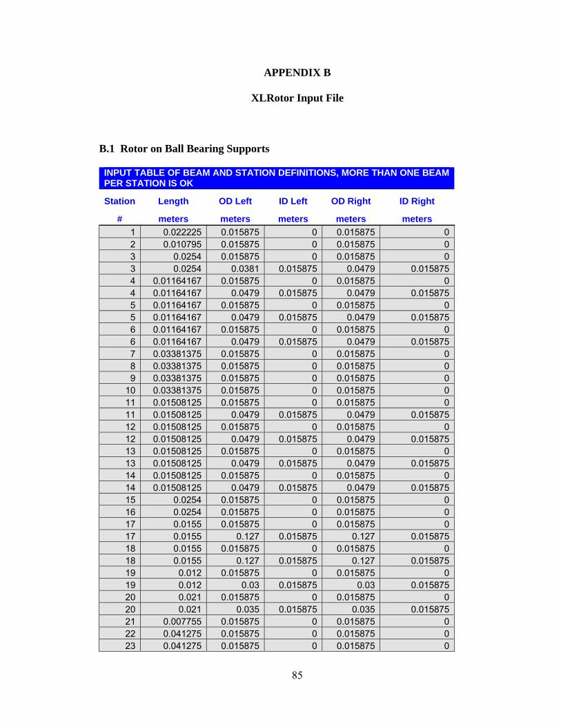
APPENDIX B
XLRotor Input File
B.1 Rotor on Ball Bearing Supports INPUT TABLE OF BEAM AND STATION DEFINITIONS, MORE THAN ONE BEAM PER STATION IS OK
Station Length OD Left ID Left OD Right ID Right
# meters meters meters meters meters 1 0.022225 0.015875 0 0.015875 0 2 0.010795 0.015875 0 0.015875 0 3 0.0254 0.015875 0 0.015875 0 3 0.0254 0.0381 0.015875 0.0479 0.015875 4 0.01164167 0.015875 0 0.015875 0 4 0.01164167 0.0479 0.015875 0.0479 0.015875 5 0.01164167 0.015875 0 0.015875 0 5 0.01164167 0.0479 0.015875 0.0479 0.015875 6 0.01164167 0.015875 0 0.015875 0 6 0.01164167 0.0479 0.015875 0.0479 0.015875 7 0.03381375 0.015875 0 0.015875 0 8 0.03381375 0.015875 0 0.015875 0 9 0.03381375 0.015875 0 0.015875 0
10 0.03381375 0.015875 0 0.015875 0 11 0.01508125 0.015875 0 0.015875 0 11 0.01508125 0.0479 0.015875 0.0479 0.015875 12 0.01508125 0.015875 0 0.015875 0 12 0.01508125 0.0479 0.015875 0.0479 0.015875 13 0.01508125 0.015875 0 0.015875 0 13 0.01508125 0.0479 0.015875 0.0479 0.015875 14 0.01508125 0.015875 0 0.015875 0 14 0.01508125 0.0479 0.015875 0.0479 0.015875 15 0.0254 0.015875 0 0.015875 0 16 0.0254 0.015875 0 0.015875 0 17 0.0155 0.015875 0 0.015875 0 17 0.0155 0.127 0.015875 0.127 0.015875 18 0.0155 0.015875 0 0.015875 0 18 0.0155 0.127 0.015875 0.127 0.015875 19 0.012 0.015875 0 0.015875 0 19 0.012 0.03 0.015875 0.03 0.015875 20 0.021 0.015875 0 0.015875 0 20 0.021 0.035 0.015875 0.035 0.015875 21 0.007755 0.015875 0 0.015875 0 22 0.041275 0.015875 0 0.015875 0 23 0.041275 0.015875 0 0.015875 0
85
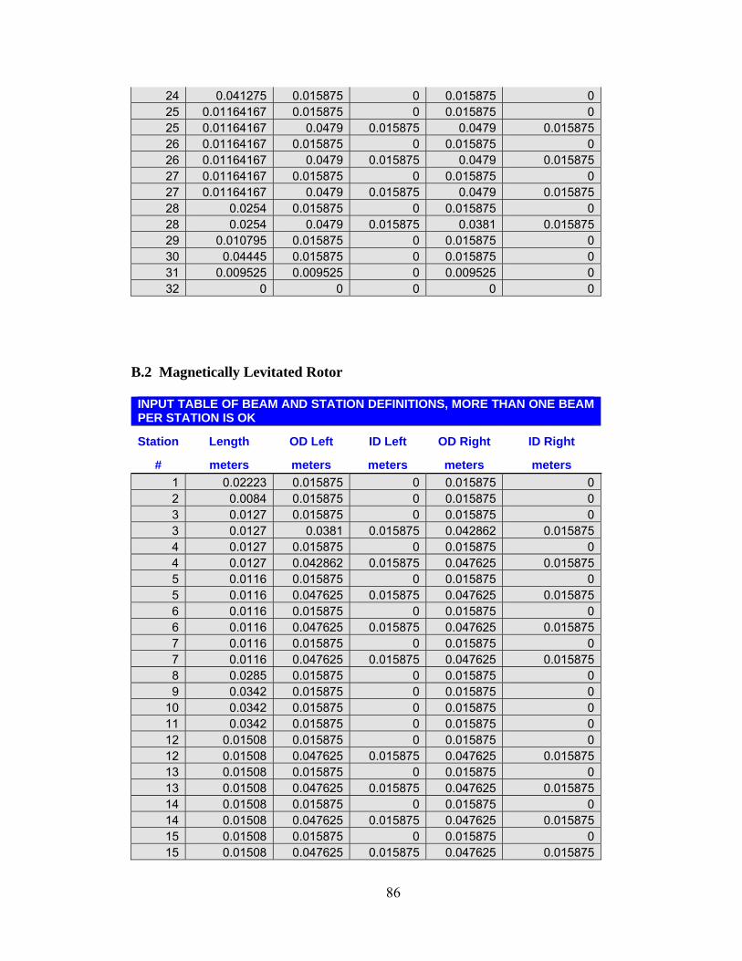
24 0.041275 0.015875 0 0.015875 0 25 0.01164167 0.015875 0 0.015875 0 25 0.01164167 0.0479 0.015875 0.0479 0.015875 26 0.01164167 0.015875 0 0.015875 0 26 0.01164167 0.0479 0.015875 0.0479 0.015875 27 0.01164167 0.015875 0 0.015875 0 27 0.01164167 0.0479 0.015875 0.0479 0.015875 28 0.0254 0.015875 0 0.015875 0 28 0.0254 0.0479 0.015875 0.0381 0.015875 29 0.010795 0.015875 0 0.015875 0 30 0.04445 0.015875 0 0.015875 0 31 0.009525 0.009525 0 0.009525 0 32 0 0 0 0 0
B.2 Magnetically Levitated Rotor INPUT TABLE OF BEAM AND STATION DEFINITIONS, MORE THAN ONE BEAM PER STATION IS OK
Station Length OD Left ID Left OD Right ID Right
# meters meters meters meters meters 1 0.02223 0.015875 0 0.015875 0 2 0.0084 0.015875 0 0.015875 0 3 0.0127 0.015875 0 0.015875 0 3 0.0127 0.0381 0.015875 0.042862 0.015875 4 0.0127 0.015875 0 0.015875 0 4 0.0127 0.042862 0.015875 0.047625 0.015875 5 0.0116 0.015875 0 0.015875 0 5 0.0116 0.047625 0.015875 0.047625 0.015875 6 0.0116 0.015875 0 0.015875 0 6 0.0116 0.047625 0.015875 0.047625 0.015875 7 0.0116 0.015875 0 0.015875 0 7 0.0116 0.047625 0.015875 0.047625 0.015875 8 0.0285 0.015875 0 0.015875 0 9 0.0342 0.015875 0 0.015875 0
10 0.0342 0.015875 0 0.015875 0 11 0.0342 0.015875 0 0.015875 0 12 0.01508 0.015875 0 0.015875 0 12 0.01508 0.047625 0.015875 0.047625 0.015875 13 0.01508 0.015875 0 0.015875 0 13 0.01508 0.047625 0.015875 0.047625 0.015875 14 0.01508 0.015875 0 0.015875 0 14 0.01508 0.047625 0.015875 0.047625 0.015875 15 0.01508 0.015875 0 0.015875 0 15 0.01508 0.047625 0.015875 0.047625 0.015875
86
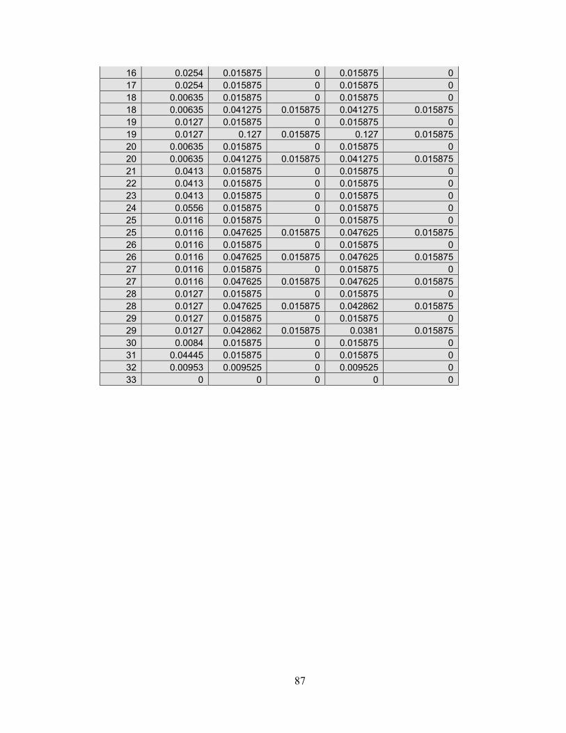
16 0.0254 0.015875 0 0.015875 0 17 0.0254 0.015875 0 0.015875 0 18 0.00635 0.015875 0 0.015875 0 18 0.00635 0.041275 0.015875 0.041275 0.015875 19 0.0127 0.015875 0 0.015875 0 19 0.0127 0.127 0.015875 0.127 0.015875 20 0.00635 0.015875 0 0.015875 0 20 0.00635 0.041275 0.015875 0.041275 0.015875 21 0.0413 0.015875 0 0.015875 0 22 0.0413 0.015875 0 0.015875 0 23 0.0413 0.015875 0 0.015875 0 24 0.0556 0.015875 0 0.015875 0 25 0.0116 0.015875 0 0.015875 0 25 0.0116 0.047625 0.015875 0.047625 0.015875 26 0.0116 0.015875 0 0.015875 0 26 0.0116 0.047625 0.015875 0.047625 0.015875 27 0.0116 0.015875 0 0.015875 0 27 0.0116 0.047625 0.015875 0.047625 0.015875 28 0.0127 0.015875 0 0.015875 0 28 0.0127 0.047625 0.015875 0.042862 0.015875 29 0.0127 0.015875 0 0.015875 0 29 0.0127 0.042862 0.015875 0.0381 0.015875 30 0.0084 0.015875 0 0.015875 0 31 0.04445 0.015875 0 0.015875 0 32 0.00953 0.009525 0 0.009525 0 33 0 0 0 0 0
87
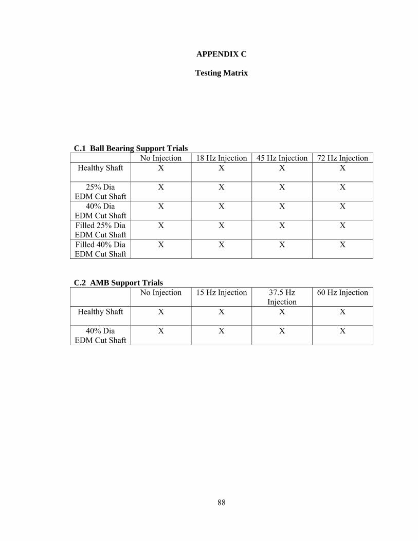
APPENDIX C
Testing Matrix
C.1 Ball Bearing Support Trials No Injection 18 Hz Injection 45 Hz Injection 72 Hz Injection
Healthy Shaft
X X X X
25% Dia EDM Cut Shaft
X X X X
40% Dia EDM Cut Shaft
X X X X
Filled 25% Dia EDM Cut Shaft
X X X X
Filled 40% Dia EDM Cut Shaft
X X X X
C.2 AMB Support Trials No Injection 15 Hz Injection 37.5 Hz
Injection 60 Hz Injection
Healthy Shaft
X X X X
40% Dia EDM Cut Shaft
X X X X
88
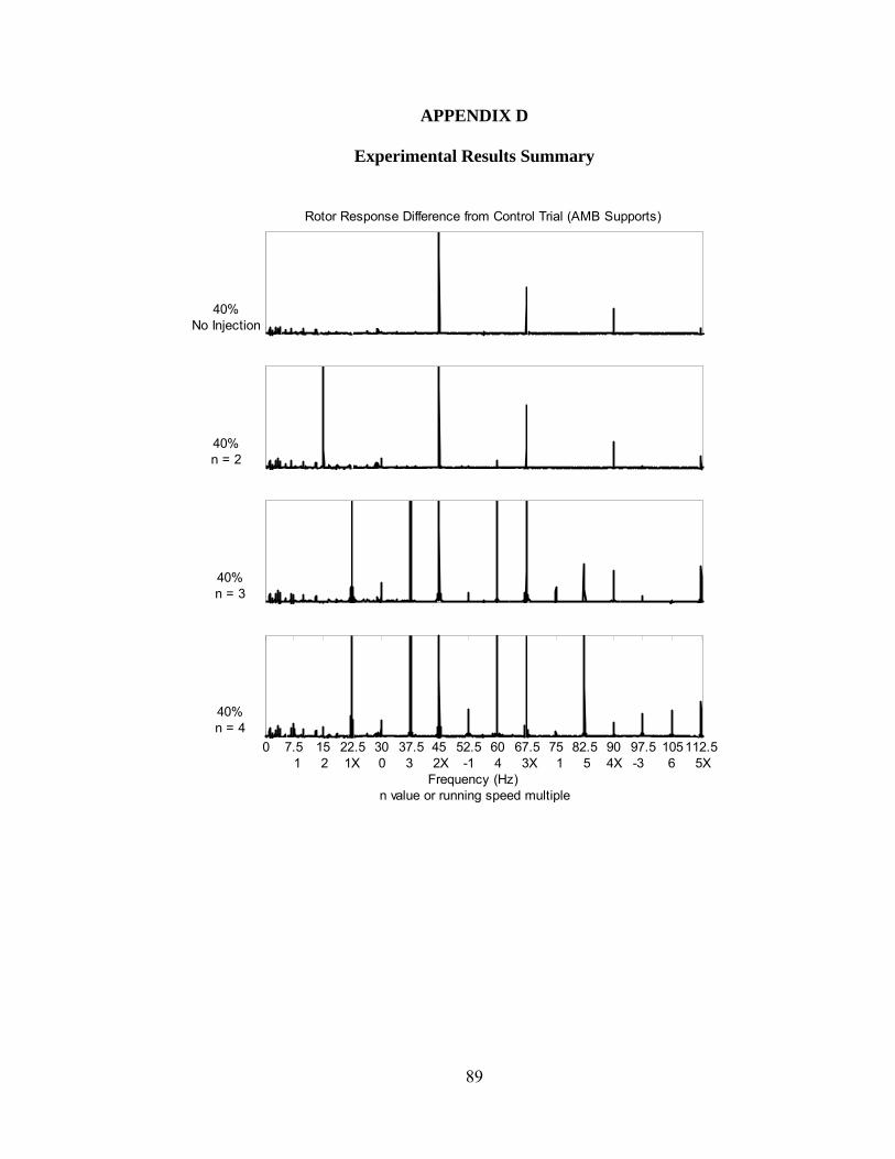
APPENDIX D
Experimental Results Summary
40%No Injection
Rotor Response Difference from Control Trial (AMB Supports)
40%n = 2
40%n = 3
0 7.5 15 22.5 30 37.5 45 52.5 60 67.5 75 82.5 90 97.5 105112.5 1 2 1X 0 3 2X -1 4 3X 1 5 4X -3 6 5X
Frequency (Hz) n value or running speed multiple
40%n = 4
89
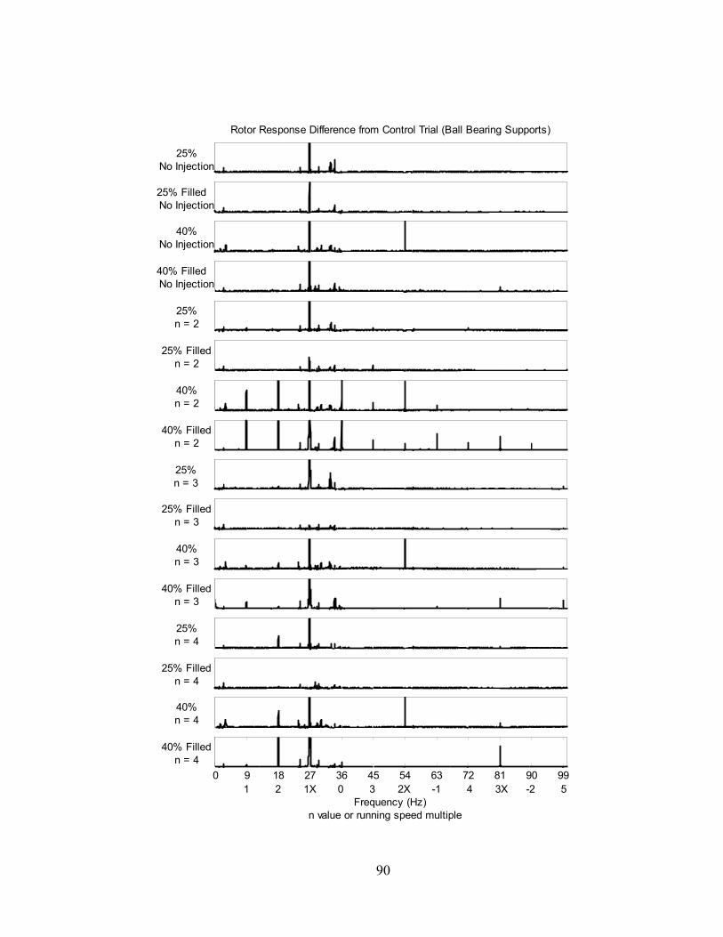
25%No Injection
Rotor Response Difference from Control Trial (Ball Bearing Supports)
25% Filled No Injection
40%No Injection
40% Filled No Injection
25%n = 2
25% Filledn = 2
40%n = 2
40% Filledn = 2
25%n = 3
25% Filledn = 3
40%n = 3
40% Filledn = 3
25%n = 4
25% Filledn = 4
40%n = 4
0 9 18 27 36 45 54 63 72 81 90 99 1 2 1X 0 3 2X -1 4 3X -2 5
Frequency (Hz) n value or running speed multiple
40% Filledn = 4
90