The Emergence of Bull and Bear Dynamics in a Nonlinear Model of Interacting Markets

Hindawi Publishing CorporationDiscrete Dynamics in Nature and SocietyVolume 2009, Article ID 310471, 30 pagesdoi:10.1155/2009/310471

Research ArticleThe Emergence of Bull and Bear Dynamics in aNonlinear Model of Interacting Markets

Fabio Tramontana,1 Laura Gardini,2 Roberto Dieci,3and Frank Westerhoff4

1 Dipartimento di Economia, Universita Politecnica delle Marche, 60121 Ancona, Italy2 Dipartimento di Economia e Metodi Quantitativi, Universita degli Studi di Urbino,61029 Urbino, Italy

3 Dipartimento di Matematica per le Scienze Economiche e Sociali, Universita di Bologna,40126 Bologna, Italy

4 Department of Economics, University of Bamberg, 96047 Bamberg, Germany

Correspondence should be addressed to Fabio Tramontana, [email protected]

Received 29 August 2008; Revised 8 February 2009; Accepted 27 March 2009

Recommended by Xue- He

We develop a three-dimensional nonlinear dynamic model in which the stock markets of twocountries are linked through the foreign exchange market. Connections are due to the tradingactivity of heterogeneous speculators. Using analytical and numerical tools, we seek to explorehow the coupling of the markets may affect the emergence of bull and bear market dynamics.The dimension of the model can be reduced by restricting investors’ trading activity, whichenables the dynamic analysis to be performed stepwise, from low-dimensional cases up to thefull three-dimensional model. In our paper we focus mainly on the dynamics of the one- and two-dimensional cases, with numerical experiments and some analytical results, and also show thatthe main features persist in the three-dimensional model.

Copyright q 2009 Fabio Tramontana et al. This is an open access article distributed under theCreative Commons Attribution License, which permits unrestricted use, distribution, andreproduction in any medium, provided the original work is properly cited.

1. Introduction

Financial market models with heterogeneous interacting agents have proven to be quitesuccessful in the recent past. For instance, these nonlinear dynamical systems have thepotential to replicate some important stylized facts of financial markets—such as theemergence of bubbles and crashes—quite well and thereby help us to understand what isgoing on in these markets. For pioneering contributions and related further developmentssee Day and Huang [1], Kirman [2], Chiarella [3], de Grauwe et al. [4], Huang and Day [5],Lux [6, 7], Brock and Hommes [8], Chiarella and He [9, 10], Farmer and Joshi [11], Chiarellaet al. [12], Hommes et al. [13], among others. Very recent surveys of this topic are providedby Hommes [14], LeBaron [15], Lux [16], Westerhoff [17], and Chiarella et al. [18].

2 Discrete Dynamics in Nature and Society

The seminal model of Day and Huang [1] reveals that nonlinear interactions betweentechnical and fundamental traders may lead to complex bull and bear market fluctuations. Thedynamics of this model, which is due to the iteration of a one-dimensional cubic map, may beunderstood with the help of bifurcation analysis. A typical route to complex dynamics may,for instance, first display a pitchfork bifurcation, followed by a cascade of period-doublingbifurcations for each of two coexisting equilibria. As a result, cycles of various periods andthen chaotic dynamics may emerge within two different regions. The two chaotic areas mayeventually merge via a homoclinic bifurcation. If that is the case, we observe apparentlyrandom switches between bull and bear markets.

In this paper we develop and explore a nonlinear model in which the stock marketsof two countries, say H(ome) and A(broad), are linked via and with the foreign exchangemarket. So far, most of these models focus on one speculative market and not much is knownabout the implications of market interactions. A few exceptions include Westerhoff [19],Chiarella et al. [20] and Westerhoff and Dieci [21]. The reason for the markets’ couplingis quite natural. Note first that stock market traders who invest abroad have to considerpotential exchange rate adjustments when they enter a speculative position. In addition, theseagents obviously need foreign currency to conduct their transactions. We assume that thereare two types of traders in the foreign exchange market. Fundamental traders believe that theexchange rate converges toward its fundamental value, and even expect that the strength ofmean reversion increases with the mispricing. Although such trading behavior tends to havea stabilizing impact on markets, it also brings nonlinearity into the model. Technical tradersoptimistically (pessimistically) continue to submit buying (selling) orders when prices arehigh (low), and thereby tend to destabilize the markets. In the absence of stock market traderswho invest abroad, the three markets evolve independently of each other. In particular, theexchange rate is driven by a one-dimensional nonlinear law of motion, and complicated bulland bear market dynamics, as observed in Day and Huang [1], may emerge.

To make matters as simple as possible, we assume that stock market traders only relyon a (linear) fundamental trading rule. If we allow stock market traders from country Ato become active in country H, then the stock market H and the foreign exchange marketare linked and coevolve in a two-dimensional nonlinear dynamical system. Our modelturns into a three-dimensional dynamical system if stock market traders from country Halso invest in country A. The expansion of the trading activity of stock market speculators,via the introduction of international connections, therefore results in a gradual increase ofthe dimension of the dynamical system. As it turns out, the bull and bear dynamics whichoriginate in the foreign exchange market spill over into the stock markets. However, there isnow also a feedback from the stock markets to the foreign exchange market, which makes thedynamics even more intricate.

A related model of interacting markets with a similar nonlinear structure was recentlyinvestigated by Dieci and Westerhoff [22] (in Dieci and Westerhoff [22], nonlinearity arisesdue to agents switching among linear competing trading rules), who focus on the nature ofthe (stabilizing or destabilizing) impact of international connections on the whole system,both in terms of local stability of the fundamental equilibrium and with regard to theamplitude of price fluctuations (in this respect, similar results on the steady-state propertieshold for the present model, too). The present paper is devoted to a quite different topic,namely the dynamic analysis of the global (homoclinic) bifurcations that mark the transitionfrom a situation with multiple equilibria to one with chaotic dynamics across bull andbear market regions, similar to that highlighted by Day and Huang [1]. As a matter offact, not much is known about such kind of dynamics in high-dimensional systems, nor

Discrete Dynamics in Nature and Society 3

about the appropriate methodology to understand their global behavior. For this reason,the dynamic analysis of our model is carried out stepwise, by introducing different levelsof interaction between markets, rendering it possible to highlight similarities and differencesin the structure of the aforementioned global bifurcations across dynamical systems ofincreasing dimension.

The two-dimensional and the full three-dimensional cases of the present model canthus be regarded as generalizations of the one-dimensional model by Day and Huang[1]. This allows us to discover and analyze the typical bull and bear dynamics in a higherdimensional context, by naturally extending the approach and techniques adopted for theone-dimensional case. Our findings and methodology may also prove to be useful forresearchers of different areas interested in homoclinic bifurcations for dynamical systems ofdimensions larger than one.

Let us describe in greater detail the key dynamic features of the model. As is wellknown, the typical bull and bear dynamics that emerge from the Day and Huang [1] model isbasically due to a sequence of local and global bifurcations involving multiple coexistingequilibria, in particular homoclinic bifurcations of repelling steady states. Such bifurcations(as well as the global structure of the basins of attraction) are closely related to thenoninvertibility of the one-dimensional cubic map used by Day and Huang [1], and to therole played by the so-called critical points (local extrema). Such kind of dynamics has beenstudied in depth for one-dimensional maps arising from a range of economic applications(see, e.g., Dieci et al. [23], He and Westerhoff [24]), often leading to analytical results. Thesame dynamic phenomena characterize the dynamics of the independent foreign exchangemarket in the one-dimensional subcase of our model. By introducing foreign traders in one ofthe stock markets, the level of integration increases, and stock price H turns out to coevolvewith the exchange rate, in a two-dimensional dynamical system. At this stage, the goal of ouranalysis is thus to show the existence of similar dynamic scenarios and global bifurcations,and to understand their mechanisms in a two-dimensional context, via a mixture of analyticaland numerical tools. Some relevant differences with the 1D case are due to the fact thatcertain symmetry properties are lost once interactions are introduced. However, the basicmechanisms behind the onset of the typical bull and bear scenario are preserved, and are stillgiven by homoclinic bifurcations of unstable (saddle) equilibria, now revealed numerically andgraphically via contacts between different kinds of invariant sets. Following Mira et al. [25]we call contact bifurcation any contact between two closed invariant sets of different kinds.A contact bifurcation may have several different dynamic effects, depending on the nature ofthe invariant sets. We recall that a homoclinic bifurcation of a cycle appears due to a contactbetween the stable and unstable set of an unstable cycle, followed by transverse intersections(i.e., followed by the existence of points which belong both to the stable and to the unstableset). The existence of a homoclinic trajectory leads to the existence of an invariant set on whichthe map is purely chaotic. There is not a unique homoclinic bifurcation, as also when a cycleis already homoclinic, further contacts and crossing can occur, leading to new homoclinictrajectories, and thus to new sets with chaotic behaviors. Moreover, since the dynamics is stillrepresented by a noninvertible map of the plane, the tool of the critical curves will prove to beuseful in fully understanding the global dynamics, including the disconnected and complexstructures of the basins of attraction.

Finally, the three-dimensional case, obtained by removing any restriction on tradingactivities across different countries, can be understood, via numerical experiments, due tothe knowledge of the dynamics occurring in the one- and two-dimensional cases. We will seethat the global bifurcations due to contacts between different invariant sets are still present,


leading to dynamics which are the natural extension to a three-dimensional space of thoseoccurring also in the two-dimensional one.

The structure of the paper is as follows. In Section 2 we derive the dynamic model,by describing the behavior of the two stock markets (Sections 2.1 and 2.2, resp.) and theforeign exchange market (Section 2.3). In Section 3 we perform a full dynamic analysis ofthe one-dimensional case. In Section 4 we consider the two-dimensional case. In particular inSection 4.1 we focus on the conditions for the local asymptotic stability of the fundamentalsteady state and on the onset of a situation of bistability. We also show how, by increasing arelevant parameter, bistability turns into coexistence of two periodic or chaotic attractors.In Section 4.2 we describe in detail the sequence of homoclinic bifurcations that lead tothe existence of a unique attractor covering two previously disjoint regions of the phasespace, and to the associated bull and bear dynamics. In Section 5 we will consider the fullthree-dimensional model. In this case the analytical results are quite poor, but we can studythe dynamics by numerical experiments, which show how the same kind of local andglobal bifurcations observed in the lower dimensional cases also occur in higher dimension,leading to similar results for the state variables of the model. Section 6 concludes this paper.Mathematical details are contained in four appendices.

2. The Model

This section is devoted to the description of the three-dimensional discrete-time dynamicmodel of internationally connected markets, which will then be analyzed in the lower dimen-sional subcases before exploring some of its properties in the full three-dimensional model.

We consider two stock markets which are linked via and with the foreign exchangemarket. The foreign exchange market is modeled in the sense of Day and Huang [1]; that is,we consider nonlinear interactions between technical traders (or chartists) and fundamentaltraders (or fundamentalists). The fraction of technical and fundamental traders is fixed,but fundamentalists rely on a nonlinear trading rule. The stock markets are denoted bythe superscript H(ome) and A(broad). For the sake of simplicity, we assume that onlyfundamental traders are active in the stock markets, with fixed proportions and linear tradingrules. Two kinds of connections exist among the markets: first, stock market traders who tradeabroad base their demand on both expected stock price movements and expected exchangerate movements. Second, in order to conduct their business they generate transactions offoreign currencies and consequent exchange rate adjustments. In each market, the priceadjustment process is simply modeled by a linear price impact function. The latter may beinterpreted as the stylized behavior of risk-neutral market makers, who stand ready to absorbthe imbalances between buyers and sellers and then adjust prices in the direction of the excessdemand.

In the following subsections we describe each market in detail.

2.1. The Stock Market in Country H

Let us start with a description of the stock market in country H. According to the assumedprice impact function, the stock price in country H (PH) at time step t + 1 is quoted as

PHt+1 = PHt + aH(DHHF,t +DHA

F,t

), (2.1)


where aH is a positive price adjustment parameter and DHHF,t , DHA

F,t reflect the orders placedby fundamental traders from countries H and A investing in country H, respectively. Forinstance, if buying orders exceed selling orders, prices go up.

The orders placed by fundamental traders from country H are given by

DHHF,t = bH

(FH − PHt

), (2.2)

where bH is a positive reaction parameter and FH is the fundamental value of stock H.Fundamentalists seek to profit from mean reversion. Hence, these traders submit buyingorders when the market is undervalued (and vice versa).

Fundamental traders from abroad may benefit from a price correction in the stockmarket and in the foreign exchange market. Denote the fundamental value of the exchangerate by FS and the exchange rate by S, then their orders can be written as

DHAF,t = cH

[(FH − PHt

)+ γH

(FS − St

)], (2.3)

where cH ≥ 0, γH > 0. Suppose, for instance, that both the stock market and the foreignexchange market are undervalued. Then the foreign fundamentalists take a larger buyingposition than the national fundamentalists (assuming equal reaction parameters). However,if the foreign exchange market is overvalued, they become more cautious (and may evenenter a selling position).

2.2. The Stock Market in Country A

Let us now turn to the stock market in country A. We have a set of equations similar to thosefor stock market H. The new stock price (PA) at time t + 1 is set as follows:

PAt+1 = PAt + aA(DAAF,t +DAH

F,t

), (2.4)

with aA > 0. The orders placed by the fundamentalists from country A investing in stockmarket A amount to

DAAF,t = bA

(FA − PAt

), (2.5)

where bA > 0 and FA is the fundamental price of stock A. The orders placed byfundamentalists from country H investing in stock market A are given as

DAHF,t = cA

[(FA − PAt

)+ γA

(1FS− 1St

)], (2.6)

where cA ≥ 0, γA > 0. Note that the latter group takes the reciprocal values of the exchangerate and its fundamental value into account.


2.3. The Foreign Exchange Market

Let us now consider the dynamics of the exchange rate (S), here defined as the price ofone unit of currency H in terms of currency A. The exchange rate adjustment in the foreignexchange market is proportional to the excess demand for currency H. The excess demand,in turn, depends not only on the stock traders who are active abroad, but also on foreignexchange speculators. The latter group of agents consists of technical and fundamentaltraders. The exchange rate for period t + 1 is

St+1 = St + d

(PHt D

HAF,t −

PAtStDAHF,t +DS

C,t +DSF,t

), (2.7)

where d is a positive price adjustment parameter. Note that the stock orders placed bythe stock traders are given in real units, so that these traders’ demand for currency is theproduct of stock orders times stock prices. In particular, PAt D

AHF,t is the demand for currency

A generated by investors from country H trading in stock market A, resulting in a demandfor currency H (of the opposite sign), given by −(PAt /St)DAH

F,t .The orders submitted by technical and fundamental speculators in the foreign

exchange market are denoted by DSC,t and DS

F,t, respectively. Following Day and Huang [1],the orders placed by chartists are formalized as

DSC,t = e

(St − FS

). (2.8)

Since e is a positive reaction parameter, (2.8) implies that chartists believe in the persistenceof bull or bear markets. For instance, if the exchange rate is above its fundamental value, thechartists are optimistic and continue buying foreign currency.

Fundamentalists seek to exploit misalignments using a nonlinear trading rule

DSF,t = f

(FS − St

)3, (2.9)

where f is a positive reaction parameter. As long as the exchange rate is close to itsfundamental value, fundamentalists are relatively cautious. But the larger the mispricing,the more aggressive they become. Day and Huang [1] argue that such behavior is justified byincreasing profit opportunities. Both the potential for and the likelihood of mean reversionare expected to increase with the mispricing.

3. The 1D Case

The complete dynamic model is given by (2.1) (combined with (2.2) and (2.3)), (2.4) (with(2.5) and (2.6)), and (2.7) (with (2.8) and (2.9)), and is represented by a 3D nonlineardynamical system. In the most simple situation, stock market traders are not allowed to trade


abroad; that is, cH = cA = 0. In this case, stock prices are independent of each other and of theexchange rate. The structure of the system is as follows:

PHt+1 = GH(PHt

),

PAt+1 = GA(PAt

),

St+1 = GS(St),

(3.1)

which is made up of three independent equations, the first two of which are linear, while thethird is cubic. It is easy to check that the two linear systems admit the respective fundamentalprices as unique steady states, which are globally stable, provided that reaction parametersare not too large, namely, aHbH < 2, aAbA < 2. The third equation, expressed in deviationsfrom fundamental value, x = (S − FS), becomes

xt+1 = φ(xt) = xt(1 + de) − dfx3t , (3.2)

and the equilibrium condition φ(x) = x for the exchange rate is the following:

x(e − fx2

)= 0, (3.3)

which always gives three equilibria for any positive value of parameters e and f . Theexchange rate dynamics produced by the third equation is similar to that described in themodel by Day and Huang [1]. In our setting, the fundamental steady state; that is, the originO (x = 0), is always unstable (φ′(0) = 1 + de > 1), while the symmetric steady statesx− := −

√e/f and x+ :=

√e/f are both stable for de < 1. In the following, the chartist demand

coefficient, e, will be chosen as the bifurcation parameter.Map (3.2) is symmetric with respect to the origin (φ(x) = −φ(−x)), so that the

bifurcations of the symmetric fixed points and cycles occur at the same value of e. Themap is bimodal: it has a local minimum at xm−1 = −

√(1 + de)/3df , at which the function

assumes a value xm0 = −2(1 + de)/3√(1 + de)/3df ; and by symmetry, a local maximum at

xM−1 = +√(1 + de)/3df , at which the function assumes a value xM0 = 2(1+de)/3

√(1 + de)/3df

(we use the notation xmi+1 := φ(xmi ) and xMi+1 := φ(xMi )). This allows us to obtain two symmetricabsorbing intervals bounded by the critical values and their images:

I− =[xm0 , x

m1

]and I+ =

[xM1 , xM0

]. (3.4)

The set of initial conditions generating bounded trajectories is the interval whose bordersare the points of an unstable 2-cycle (α−, α+) (see Figure 1(a)). By taking an initial condition(i.c. henceforth) below α− or above α+, the exchange rate diverges, while in the other cases itconverges to one of the attractors located in the absorbing intervals. The immediate basin ofattraction of the positive fixed point x+ is bounded by the fundamental steady state and by itspositive rank-1 preimage, B+0 :=]O,O+

−1[. The immediate basin is not the only interval whosepoints generate trajectories converging to the positive steady steate. In fact, B+0 has a preimageformed by negative values, B+−1, which has a preimage B+−2 inside interval ]O+

−1, α+[ . The


−4 4O

4

−4

x−

x+

xt

α+

α−

f(xt)

f2(xt)

(a)

O 2 4

4

2

f(xt)

f2(xt)

x+xM1

xM0I+

O+−1

α+

xt

(b)

Figure 1: Stable non-fundamental steady states. (a) and its enlargement (b) are obtained using thefollowing set of parameters: d = 0.35, e = 2.687, and f = 0.7.

−4 4

4

−4

f(xt)

xt

O+−1

O−−1

O+−2

B+−2

B+0

B+−1

(a)

2.7 3.5

3.5

2.7

O+−3

O−−2

O+−1

α+

B+ B−

(b)

Figure 2: Basins of attraction. In (a) the immediate basin of the steady state x+ and its rank-1 and rank-2 preimages are represented in blue. In (b) an enlargement of the interval between O−1

+ and α+ with thealternance of intervals belonging to the basin of attraction of x+ (in blue) and x− (in green) are shown. Theparameters are as in Figure 1.

latter, in turn, has a preimage in the negative values, and so on (Figure 2(a)), thus formingan infinite sequence of intervals, which are all part of the basin of attraction of x+ and thataccumulate at the points of the unstable 2-cycle (α−, α+). Such intervals alternate on the realline with the intervals belonging to the basin of x−, determined in a similar way. The bordersof the intervals are given by the preimages of the fundamental steady state (Figure 2(b)). Theunion of the infinitely many intervals is the basin of attraction of x+:

B+ := B+0⋃B+−1

⋃B+−2

⋃..., (3.5)

and an analogous (and symmetric) explanation holds for the basin of the negative steadystate, B−.


O 2 4

4

2

f(xt)

f2(xt)

xM1

xM0

I+

α+

xt

(a)

2 4

4

2

f(xt)

f2(xt)

xt

(b)

Figure 3: Periodic and chaotic attractors. In (a) a stable 2-cycle is obtained using the same set of parametersof Figure 1 except for e = 3.483. In (b) the chaotic attractor is obtained with e = 3.7436.

f(xt)

f2(xt)

2 4

4

2

xt

Figure 4: Homoclinic bifurcation of x+. The two chaotic intervals around x+ merge into a unique chaoticinterval for e � 3.89. The remaining parameters are as in Figure 3.

For de > 1, steady states x− and x+ become unstable via flip-bifurcation (as φ′(x+) =φ′(x−) = 1−2de = −1 for de = 1). By increasing the value of e, the dynamics show a cascade offlip bifurcations, finally leading to chaos (Figure 3). In these cases, B+ and B− are the basins ofattraction of the periodic cycles or the chaotic intervals located in I+ and I−, respectively. Fore � 3.89, the chaotic intervals included in I+ merge into a unique chaotic interval (Figure 4).The same happens for the chaotic intervals in I−, for the symmetry properties of the map. Thisis a remarkable global bifurcation, namely, a homoclinic bifurcation ofx− (and symmetricallyx+), occurring when the third iterate of the critical point merges with the unstable fixed point.Before this bifurcation, the asymptotic dynamics can only consist of cycles of even periods,whereas cycles of odd periods will appear after it. Moreover, this is the first parameter valueat which the dynamics is chaotic on one interval (in the sense of chaos of full measure on aninterval).


f(xt)

−4 O 4

4

xM1 = xm1

−4α−

xm0

α+xM0

xt

Figure 5: Homoclinic bifurcation of O. The two chaotic intervals around x+ and around x− merge into aunique chaotic interval for e � 4.5659 . The remaining parameters are as in Figure 4.

x

−4.2

0

4.2

e

0 3.89 4.57 5.75 6

Figure 6: Bifurcation diagram versus parameter e for the one-dimensional model, under the basicparameter setting: d = 0.35 and f = 0.7. The homoclinic bifurcation of the two symmetric fixed pointsoccurs at e � 3.89, the reunion of the two disjoint intervals, homoclinic bifurcation of the origin, ate � 4.5659, while the final bifurcation occurs at e = ef � 5.75.

Figures 3 and 4, which are restricted to the upper right branch of the map, describe thedynamics and the structure of the attractors around the steady state x+. To understand theglobal dynamics, we must consider the other portion, too. The global structure of the basinsis similar to that described above (Figure 2) for the case of coexisting stable steady states; thatis, each basin consists of infinitely many intervals with the unstable two-cycle (α−, α+) as thelimit set. Thus taking the i.c. on the right or the left of the origin is not a sufficient conditionfor convergence to the attractor on that side. For the points close to the two-cycle (α−, α+) inparticular it is almost impossible to say whether there will be convergence to the attractor onthe right or on the left. However, the two attractors (and their basins) will merge together forhigher values of the parameter e. A further rise in the value of e takes xm1 and xM1 increasingly


closer to the fundamental steady state, and increasingly closer to each other. As long as xm1 < 0and xM1 > 0, the two absorbing intervals are still separated, but at e = (3

√3/2 − 1)(1/d) , xm1

and xM1 merge in x = 0. Each trajectory starting from interval ]xm0 , xM0 [ now covers the whole

interval I− ∪ I+ = [xm0 , xM0 ] (homoclinic bifurcation of O). The basin of the enlarged invariant

interval I− ∪ I+ is the whole interval B :=]α−, α+[ (Figure 5).Put differently, the two disjoint symmetric attractors exist as long as each unimodal

part of the map behaves as the standard logistic map, xt+1 = fμ(xt) = μxt(1 − xt),for 3 < μ < 4. The global bifurcation occurring in the logistic map at μ = 4 (firsthomoclinic bifurcation of the origin O) followed by diverging trajectories, is replaced hereby a homoclinic bifurcation leading to the reunion of the two chaotic attractors. This is betterillustrated in the bifurcation diagram in Figure 6. An i.c. in the immediate basin on the righttends to the attractor on the positive side (in red in Figure 6), while an i.c. in the immediatebasin on the left tends to the attractor on the negative side (in blue in Figure 6). At thehomoclinic bifurcation of the origin we observe their reunion: there is a unique attractor (ingreen in Figure 6) and any point belonging to interval B :=]α−, α+[ tends toward it.

This kind of dynamics persists as long as the chaotic interval is inside the repellingtwo cycle; that is, [xm0 , x

M0 ] ⊂]α−, α+[. It is clear that the lastor final bifurcation here occurs at a

value e = ef , at which xm0 = α− (and clearly also xM0 = α+), that is

−2(1 + de)3

√1 + de

3df= α−(e) ,

2(1 + de)3

√1 + de

3df= α+(e) (3.6)

In Appendix A we show that xM0 (e) tends to infinity faster than α+(e) so that a finitevalue of e exists, say ef , leading to the final bifurcation (3.6). As for the logistic map, afterthis final bifurcation the generic trajectory is divergent (and thus the model is no longermeaningful). However, an invariant chaotic set inside interval [xm0 , x

M0 ] still exists for any

larger value of e: a so-called chaotic repellor, which represents the only surviving boundedinvariant set. Summarizing, we have proven the following.

Proposition 3.1. The bimodal map in (3.2) is symmetric with respect to the origin, with alocal maximum point at xM−1 = +

√(1 + de)/3df and local maximum value xM0 = (2(1 +

de))/3√(1 + de)/3df . An unstable fixed point in the origin always exists. A positive fixed point

x+ =√e/f is locally asymptotically stable for de < 1. A flip bifurcation of x+ occurs at de = 1.

The attracting set on the half-line x > 0 is included in the absorbing interval I+ = [xM1 , xM0 ] for0 < e < (3

√3/2 − 1)(1/d), disjoint from the symmetric one, on the half-line x < 0, and the basins

of the two disjoint invariant sets consist of infinitely many intervals, having the unstable 2-cycle withperiodic points ( α−, α+) as limit set. At e = (3

√3/2−1)(1/d) the homoclinic bifurcation of the origin

occurs, and for (3√

3/2 − 1)(1/d) < e < ef the dynamics are bounded in the interval [xm0 , xM0 ]. For

e > ef the generic trajectory is divergent.

From an economic point of view it is interesting to note that already the one-dimensional nonlinear map for the foreign exchange market is able to generate endogenousdynamics (i.e., excess volatility) and bubbles and crashes. For a more detailed economicinterpretation of this scenario see the related setup of Day and Huang [1]. An interestingquestion is whether this kind of dynamic behavior may survive in a higher dimensionalcontext; for example, when the foreign exchange market is coupled with a stock market.A first answer is provided in the following section.


4. The 2D Case

In this section we analyze the case in which stock market traders from H are not allowedto trade in A; that is, cA = 0, while stock market traders from A are allowed to trade in H,cH > 0. In this case, stock market A decouples from the other two markets and is drivenby an independent linear equation PAt+1 = GA(PAt ) (whose dynamical properties were brieflydiscussed in the previous section). We thus have an independent two-dimensional systemwith the following structure:

PHt+1 = GH(PHt , St

),

St+1 = GS(PHt , St

).

(4.1)

System (4.1) expressed in deviations (although we work with deviations, in all the followingnumerical experiments we have checked that original prices never become negative) fromfundamental values, x = (PH − FH) and y = (S − FS), is driven by the map T : R

2 → R2

defined as follows:

T :

⎧⎨⎩xt+1 = xt − aH

[(bH + cH

)xt + cHγHyt

],

yt+1 = yt − d[cH(xt + FH

)(xt + γHyt

)− eyt + fy3

t

].

(4.2)

4.1. Steady States and Multistability

With regard to system (4.2), the equilibrium conditions for the stock price in country H andthe exchange rate are given, respectively, by

x

[f

(qH)3x2 + bHx + bHFH − e

qH

]= 0, (4.3)

y = − x

qH, (4.4)

where qH := cHγH/(bH + cH). Apart from the fundamental steady state, say O, representedby x = 0 and y = 0, two further equilibria (denoted as P1 and P2) may exist, provided that

e > eSN :=−(bH)2(

qH)4

4f+ bHFHqH. (4.5)

For e = eSN , the unique additional solution to (4.3) is given by x = (−bH(qH)3)/2f < 0, whichmeans that when e increases beyond the bifurcation value eSN , the newborn non-fundamentalsteady states are initially characterized by x < 0 (equilibrium price H below fundamental)and y > 0 (equilibrium exchange rate above fundamental).

Three steady states therefore coexist when the reaction parameter e (which measureschartists’ belief in the persistence of bull and bear markets) is large enough. Although thisscenario of multistability in the 2D model of interconnected markets is similar to that of the


y

x

O

P2

P1

−0.002

0

0.014

−0.0065 0 0.0035

(a)

y

x

O

P2

P1

−3.7

0

3.8

−2.5 0 2.5

(b)

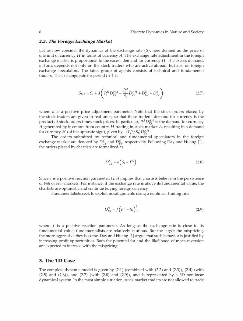
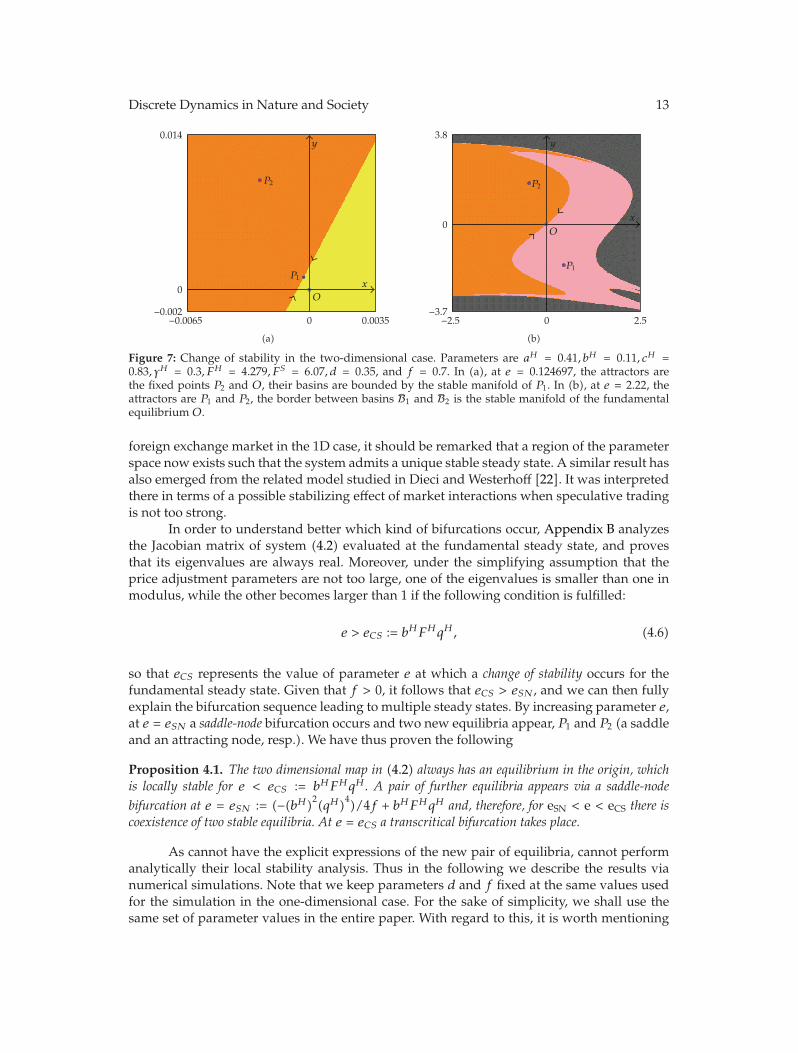
Figure 7: Change of stability in the two-dimensional case. Parameters are aH = 0.41, bH = 0.11, cH =0.83, γH = 0.3, FH = 4.279, FS = 6.07, d = 0.35, and f = 0.7. In (a), at e = 0.124697, the attractors arethe fixed points P2 and O, their basins are bounded by the stable manifold of P1. In (b), at e = 2.22, theattractors are P1 and P2, the border between basins B1 and B2 is the stable manifold of the fundamentalequilibrium O.

foreign exchange market in the 1D case, it should be remarked that a region of the parameterspace now exists such that the system admits a unique stable steady state. A similar result hasalso emerged from the related model studied in Dieci and Westerhoff [22]. It was interpretedthere in terms of a possible stabilizing effect of market interactions when speculative tradingis not too strong.

In order to understand better which kind of bifurcations occur, Appendix B analyzesthe Jacobian matrix of system (4.2) evaluated at the fundamental steady state, and provesthat its eigenvalues are always real. Moreover, under the simplifying assumption that theprice adjustment parameters are not too large, one of the eigenvalues is smaller than one inmodulus, while the other becomes larger than 1 if the following condition is fulfilled:

e > eCS := bHFHqH, (4.6)

so that eCS represents the value of parameter e at which a change of stability occurs for thefundamental steady state. Given that f > 0, it follows that eCS > eSN , and we can then fullyexplain the bifurcation sequence leading to multiple steady states. By increasing parameter e,at e = eSN a saddle-node bifurcation occurs and two new equilibria appear, P1 and P2 (a saddleand an attracting node, resp.). We have thus proven the following

Proposition 4.1. The two dimensional map in (4.2) always has an equilibrium in the origin, whichis locally stable for e < eCS := bHFHqH . A pair of further equilibria appears via a saddle-nodebifurcation at e = eSN := (−(bH)2(qH)4)/4f + bHFHqH and, therefore, for eSN < e < eCS there iscoexistence of two stable equilibria. At e = eCS a transcritical bifurcation takes place.

As cannot have the explicit expressions of the new pair of equilibria, cannot performanalytically their local stability analysis. Thus in the following we describe the results vianumerical simulations. Note that we keep parameters d and f fixed at the same values usedfor the simulation in the one-dimensional case. For the sake of simplicity, we shall use thesame set of parameter values in the entire paper. With regard to this, it is worth mentioning


P2

P1

y

−4

4

e

0.1 4

(a)

P2

P1

e2e1

y

−2.5

2.5

e

2 2.7

(b)

Figure 8: Bifurcation diagrams (b.d. for short). In blue the b.d. corresponding to an initial condition closeto P1, whereas the b.d. in red is obtained with an initial condition close to P2. Panel (b) is a magnificationof a portion of the b.d. in (a), which emphasizes the values of parameter e at which the steady states losestability.

that for alternative parameter settings we have observed the same kind of dynamics andbifurcations as described in what follows.

Of the two new equilibria, the stable one, which we call P2, is the one further from thefundamental equilibrium. For values of parameter e in the range eSN < e < eCS were we havecoexistence of two stable equilibria, the fundamental O coexists with the equilibrium pointP2. The points of the phase plane either converge toO or to P2, and the two basins of attractionare separated by the stable set of the saddle equilibrium point P1. An example is shownin Figure 7(a), where we use the following parameter setting: aH = 0.41, bH = 0.11, cH =0.83, γH = 0.3, FH = 4.279, FS = 6.07, d = 0.35, and f = 0.7.

At e = eCS the fixed point P1 merges with the fundamental one and then crosses it,and the stability properties of the two steady states changes too (transcritical bifurcation).It is worth noting that the range of values (eSN, eCS) of parameter e between the saddle-node bifurcation and the transcritical bifurcation becomes increasingly smaller as f increases(compare equations (4.5) and (4.6)). For values of parameter e > eCS and close to thebifurcation, the fundamental equilibrium O is unstable while the two equilibria P1 and P2

are both stable. The stable set WSO of the saddle O is the separator between the two basins

of attraction, B1 and B2, respectively, while the two branches of the unstable set WuO have

opposite behavior: one tends to attractor P1 while the other tends to attractor P2. An exampleis shown in Figure 7(b).

As parameter e is further increased, both equilibria P1 and P2 become unstable viaa flip (or period doubling) bifurcation. Moreover, a cascade of flip bifurcations, leading tochaos, will take place for both of them. However, unlike the results in the 1D model, the twosequences of flip bifurcations are not synchronized, due to the asymmetry of the 2D map.An example is shown in the bifurcation diagram of Figure 8. By fixing all parameters, exceptfor e, we can see that equilibrium P1 first undergoes a flip bifurcation at e = e1 and thenP2 at e = e2 > e1. In the narrow range e1 < e < e2 the points of the phase plane eitherconverge to the stable equilibrium P2 or to a stable 2-cycle born from the flip bifurcation ofP1 and close to it. The two basins B1, and B2 are always separated by the stable set WS

O ofthe saddle fundamental equilibrium O, while the two branches of the unstable set Wu

O of thefundamental equilibrium behave in an opposite manner: one tends to equilibrium P2 andthe other to the attractor born from P1. As parameter e increases, we observe several flip


bifurcations associated with the two attractors, say A1 and A2, while their basins B1, andB2 are always separated by the stable set of O. The two branches of the unstable set of Ostill converge to the two different attractors until certain global bifurcations occur, as we willdescribe below. Also the structure of the attractors and that of the two basins undergo globalbifurcations.

Although the two attractors A1 and A2 are not steady states, the long-run dynamicsof the system still takes place in the same regions as that represented in Figure 7(b). In fact,the asymptotic states are either in region y < 0, x > 0, denoted as the bear region (whenorbits converge to A1) or in region y > 0, x < 0, denoted as the bull region (when orbitsconverge toA2). In the bear (bull) region, the exchange rate is below (above) its fundamentalvalue, whereas stock price H is above (below) the fundamental value. An example is shownin Figure 9(a), where two 4-cycles coexist, while in Figure 9(b) two chaotic attractors coexist,both formed by two separate chaotic areas. However, the structure of the basins of attractionB1 and B2 becomes much more complicated. They are disconnected, which is a consequenceof the noninvertibility of the map. More precisely, for noninvertible maps the phase planemay be subdivided into regions of points having the same number of rank-1 preimages. Theseregions are separated by the critical curve LC, also shown in Figure 9 together with the locusLC−1, where LC = T(LC−1) (see Appendix C). When the parameter e changes, a portion ofa basin of attraction may cross some arc of curve LC, thus entering inside a region with ahigher number of preimages. This contact bifurcation causes the appearance of disconnectedportions of the basin of attraction. An example is given by portion H of basin B1 of attractorA1 (located near P1), which is shown to exist in Figure 9(b) but not yet in Figure 9(a). Thecreation of this disconnected region is due to the small portion H ′ of basin B1 which hasmoved in Figure 9(b) to the left of LC (see arrow in Figure 9(b)), thus entering a region of thephase space whose points have a higher number of preimages. Two new rank-1 preimages ofH ′, appearing on opposite sides of LC−1, create the disconnected portion of basin labelled H.

4.2. Global Bifurcations

The previous subsection has shown how, under increasing values of parameter e, the twoattractors (first equilibria P1 and P2 thenA1 andA2) undergo a sequence of flip bifurcationswhich is not synchronized, leading the system to chaotic dynamics. The sequence of flipbifurcations can also be observed in Figure 10. From Figure 10 the existence of differentintervals for parameter e can be noted, such that the dynamics in the phase plane arequalitatively the same within each range. Such intervals are denoted as A, B, C, D, and E. Theborders between two adjacent intervals are associated with homoclinic bifurcations involvingone or two of the three equilibria, and will be described in the present subsection.

4.2.1. First Homoclinic Bifurcation of P1 and P2

As stated above, for a wide interval of values of e, we observe two coexisting attractorsAi, i = 1, 2, each consisting of two parts. The dynamics on each attractor alternately jumpsfrom one to the other side of the stable set WS

Piof the saddle Pi. The first global bifurcation

occurring to the chaotic area is caused by the contact between the two parts constitutingthe chaotic attractor Ai and the stable manifold WS

Pi, leading to a one-piece chaotic area Ai.

This corresponds to the first homoclinic bifurcation of the saddle equilibria Pi. This bifurcationis the two-dimensional analogue of that occurring in the 1D case, described in Section 3,


y

x

O

P2

LC

LC LC−1

LC−1

P1

−3.7

0

3.8

−2.5 0 2.5

(a)

y

x

O

P2LC

LCLC−1

LC−1

H

H ′

P1

−3.7

0

3.8

−2.5 0 2.5

(b)

Figure 9: Basins of attraction. Basin B1 of the attractor located around P1 is in pink, whereas basin B2,whose points lead to the attractor around P2, is in orange. In (a), for e = 3.43, attractorsA1 andA2 are twocoexisting 4-cycles. In (b), for e = 3.56, the attractors are two coexisting two-piece chaotic attractors.

P1

y

−3.8

0

3.8

e

3.3 5.2A B C D E

e1 (AB)

e1 (BC)

e2 (CD)

e (DE)

(a)

P2

y

−3.8

0

3.8

e

3.3 5.2A B C D E

e2 (AB)

e1 (BC)

e2 (CD)

e (DE)

(b)

Figure 10: Bifurcation diagrams. The b.d. in (a) corresponds to an initial condition close to P1, whereas theb.d. in (b) assumes an initial condition close to P2. The green portion of the diagrams is the same for anyinitial condition (except for those leading to divergent trajectories).

Figure 4. The latter was due to a contact between a critical point on the boundary of the chaoticinterval and the unstable steady state. Here we have a contact between arcs of critical curves,which constitute the boundary of the chaotic attractor (see Mira et al. [25]), and the stableset of the saddle. From Figure 10 we can see that such global bifurcations also occur in anasynchronous manner: at e = e1

(AB) we first observe it for P1, and it then occurs for P2 ate = e2

(AB) > e1(AB). In Figure 11(a), which shows the homoclinic bifurcation of P1, the value of

e is approximately e1(AB)

∼= 3.6. Just after this global bifurcation, for e > e1(AB) but still close to

the bifurcation value, attractorA1 is a one-piece chaotic area. An interesting feature related tothis homoclinic bifurcation is that the boundary of the chaotic attractor is no longer made upof only segments of critical curves, but includes both portions of critical curves and portionsof the unstable manifold Wu

P1of saddle point P1 (a so-called mixed-type boundary,as described

in Mira et al. [25]). This is highlighted in Figure 11(b). Clearly, the same kind of bifurcation


P1

WSP1

WuP1

y

−2.78

−0.76

x

0.418 0.6

(a)

P1

WuP1

WuP1

LC

LC

LC

y

−2.9

−0.4

x

0.4 0.65

(b)

Figure 11: First homoclinic bifurcation of P1. (a) shows the contact between the two pieces of attractorA1and the stable set Ws

P1, at the bifurcation value e = e1

(AB) = 3.6. (b) portrays the one-piece chaotic area A1

after the bifurcation, at e = 3.65, whose boundary is made up of pieces of both critical lines (denoted asLC) and unstable manifold (Wu

P1).

occurs at e = e2(AB), involving the stable set WS

P2of saddle equilibrium point P2 and leading to

a one-piece chaotic areaA2.

4.2.2. Second Homoclinic Bifurcation of P1 and P2, and Homoclinic Bifurcation of O

For e > e2(AB), the two chaotic areas include the saddle equilibria Pi on their border. These

saddle points only have homoclinic points on one branch of their stable set: the one whichis inside the chaotic area. A second homoclinic bifurcation of the equilibria Pi will occur athigher values of e, involving the other side of the stable set of saddles Pi, and leading totwo other global bifurcations, whose effects are even more dramatic with respect to the firstone. As expected, the two bifurcations do not occur simultaneously. Instead, as we shall see,each of these secondary homoclinic bifurcations of saddles Pi is simultaneous to a homoclinicbifurcation of the saddle equilibrium O, involving one and then the other side of its unstableset, respectively. First the homoclinic bifurcation of P1 occurs, at e = e1

(BC), leading to the“disappearance” of the chaotic attractor A1 (and leaving A2 as the unique attracting set).Then the homoclinic bifurcation of P2 occurs, at e = e2

(CD) > e1(BC), leading to the “explosion”

of the chaotic attractorA2. Let us describe this sequence in our example.By increasing parameter e, for e > e2

(AB) the chaotic attractors become increasinglylarger, until one of them has a contact with the frontier between its basin of attraction and thatof the coexisting attractor. The first contact occurs at e = e1

(BC) (� 4.198), involving equilibriumpoint P1, which is shown in Figure 12(a). We can see that tongues of basin B2 have reachedthe boundary of chaotic area A1, and are accumulating along the branch of stable set WS

P1.

This means that the unstable set WuP1(on the frontier of the chaotic areaA1) and the stable set

WSP1(whose points are accumulating on the frontier of basin B1) are at the second homoclinic

tangency of P1 (which will be followed by transverse crossing). In the meantime, we cansee that tongues of chaotic area A1 (whose boundary consists of limit points of the unstableset Wu

O of the fundamental equilibrium) have reached the boundary of the basin and havecontacts with the stable set of the origin,WS

O. We are therefore at the first homoclinic tangency


y

x

O

P2

P1

WuO

WSO Wu

P1

−3.51

0

4.83

−1.72 0 1.15

(a)

y

x

O

P2

P1

WuO

WSO

−3.51

0

4.83

−1.72 0 1.15

(b)

Figure 12: One-side homoclinic bifurcation of O. (a) shows the situation at the bifurcation value e � 4.198,while (b) portrays a situation just after the bifurcation, at e = 4.2.

of O (which will be followed by transverse crossing). This is not a surprising situation butthe standard mechanism, due to the fact that homoclinic points involve the whole stable setWS

P1external to the chaotic area, and this branch is related to the frontier. This means that,

besides the two homoclinic bifurcations occurring simultaneously at e = e1(BC), heteroclinic

connections and heteroclinic loops between the two equilibria P1 and O also occur. The effectof this bifurcation is “catastrophic:” the chaotic attractor A1 disappears, becoming a chaoticrepellor. For e = e1

(BC), the unique attractor A2 is left (see Figure 12(b)). For values of e notfar from this bifurcation, convergence to the unique attractor may be very slow. This is dueto the existence of the chaotic repellor (in the same region previously covered by chaoticarea A1) and before convergence the system may exhibit a kind of chaotic behavior alongthe ”ghost” of the old chaotic attractor A1 (sometimes it takes about 100 000 time periodsbefore convergence to the new chaotic area A2 can be observed). We remark that, startingfrom initial conditions close to P2, converging to A2, we cannot detect any differences inthe dynamic behavior before and after this bifurcation, because the latter involves only theother attractor A1. This is clearly a global bifurcation of basin of attraction B2. In fact, atthis bifurcation, the previous two basins merge into a unique one (see Figure 12(b)); that is,basin B2 becomes much wider and its frontier separates the points of the phase plane havingbounded trajectories from those generating divergent trajectories (basin B∞). However, itis worth noting that the numerically obtained picture of basin B2 also includes all of therepelling cycles existing in the chaotic repellor, as well as its stable set. Namely, the coloredarea representing B2 in Figure 12(b) also contains the unstable equilibria O and P1 withtheir stable sets, as well as infinitely many other cycles, all belonging to an invariant setcharacterized by chaotic dynamics which, however, has measure zero in the phase plane, sothat it is not detectable in practice from the iterated points. The existence of a strange repellor,besides affecting the chaotic transient, as observed above, also causes another remarkablehomoclinic bifurcation involving the chaotic areaA2. In fact, as e increases, we approach thesecond homoclinic bifurcation of saddle P2, which is located on the boundary of the chaoticattractor. This bifurcation involves the branch of the stable set external to the chaotic area,and at the same time it also represents the second homoclinic bifurcation of the fundamentalequilibriumO. The parameter bifurcation value is e = e2

(CD), at which chaotic areaA2 becomestangent to the left-hand side of the stable set Ws

O of the fundamental equilibrium O (as can be


y

x

O

P2

P1

−4

0

3.5

−2.5 0 2.5

(a)

y

x

P2

P1

−4

0

3.8

−2.5 0 2.5

(b)

Pric

eH

(dev

iati

onfr

omfu

ndam

enta

l)

−1.5

−1

−0.50

0.5

1

1.5

Time

200 250 300 350 400

(c)

Exc

hang

era

te(d

evia

tion

from

fund

amen

tal)

−6

−4

−2

0

2

4

6

Time

200 250 300 350 400

(d)

Figure 13: Homoclinic bifurcation of O and final bifurcation. In (a), we take e = 4.3, while in (b) e = 4.893.The points that will be involved in the contact between the strange attractor and the basin boundary caneasily be guessed. In (c) and (d) we represent the dynamics of the state variables x and y in the timedomain, switching between bull and bear markets, for e = 4.75.

argued from Figure 13(a), at a value of e just after the bifurcation). Again, though not visiblefrom the figure, this occurs simultaneously to the homoclinic bifurcation involving the stableset Ws

P2and the unstable set Wu

P2, and is also related to the heteroclinic connections between

the fixed point P2 and the fundamental steady state O. The appearance of such homoclinicorbits is revealed from the dynamic effect occurring at the bifurcation. This results in a suddenincrease of the chaotic area, which now also covers that of the chaotic repellor (which isincluded in the wider chaotic area).

The asymmetry of the map implies that the contacts between the chaotic attractorsand the stable manifold of O do not occur at the same time. In our example, for valuesof e such that e1

(BC) < e < e2(CD), the asymptotic dynamics of the exchange rate usually

take place above the fundamental value, while the asymptotic values of stock price H arelower than the fundamental price. This dynamic behavior changes drastically at the globalbifurcation occurring at e = e2

(CD), leading to an explosion of the chaotic area. In general, fore < e2

(CD) the asympotic behavior is approximately on one side of the fundamental. Apartfrom initial conditions taken in B∞, the asymptotic dynamics occur (approximately) either inthe bear region (the second quadrant, x > 0, y < 0) or in the bull region (the fourth quadrantx < 0, y > 0) (there may indeed be some points of the attractors located in the first or thirdquadrants). In contrast, for values of parameter e larger than e2

(CD), the asymptotic dynamicstake place across both quadrants, and switches from one to the other at unpredictable points


y

x

O

P2

P1

C1

C2

−4.5

0

4.5

−10 0 6.5

(a)

y

x

O

P2

P1

C1

C2

−4.5

0

4.5

−10 0 6.5

(b)

Figure 14: Homoclinic bifurcation of O and final bifurcation. In (a), the value of e is 4.893 , while in (b)e = 5.05.

in time. After the bifurcation, but for e close enough to the bifurcation value, almost allrealizations will be on the fourth quadrant (see Figure 13(a)), and only rare transitions to thearea previously occupied by the chaotic repellor are observed. When e is sufficiently large, thenumber of iterations on each region and the number of switches becomes more frequent andtotally unpredictable, so that the density of points in the two regions is the same on average(see Figure 13(b)). But differently, both regions become relevant to the dynamics in the timedomain. Figures 13(c), 13(d) represent time paths of state variables x and y, obtained with avalue of parameter e larger than its second homoclinic bifurcation value e2

(CD).We remark that in the interval of values of e where a unique attractor exists (that is, for

e > e2(CD)), before the last homoclinic bifurcation (final bifurcation) described in what follows,

several other periodic windows may arise, each related to a local bifurcation causing theappearance, in pairs, of a cycle saddle and a node, followed by a cascade of local and globalbifurcations similar to those described earlier for the fixed points. Two periodic windowsrelated to cycles of period 3 are clearly visible in the bifurcation diagram of Figure 10.However, as e increases, the dominant dynamics is chaotic behavior across the whole area.

From an economic perspective our findings imply that the famous bull and bearmarket dynamics first described by Day and Huang [1]— and also observed in the previoussection—may indeed survive an extension to a higher dimensional context. However, pricefluctuations may become even more intricate since now there is an additional (irregular)feedback from the stock market to the foreign exchange market. In addition, we see that anotherwise stable stock market may display complex endogenous dynamics when coupledwith an unstable foreign exchange market.

4.2.3. Final Bifurcation

So far, we have observed several homoclinic bifurcations involving the chaotic area. It isworth noting that the homoclinic bifurcations occurring at e = e1

(AB) and e = e2(AB) are also

called interior crises in Grebogi et al. [26]. The reason for this is clearly related to their dynamiceffect, while the bifurcations occurring at e = e1

(BC) and e = e2(CD) are also called exterior crises,

again in relation to their dynamic effect. Now let us describe the so-called final bifurcation,


P1

x

−4.2

0

4.2

e

0 5.6ep ef1 eh1 eg1 eg2 ef

(a)

P2x

−4.2

0

4.2

e

0 5.6ep ef2 eh2 eg2 ef

(b)

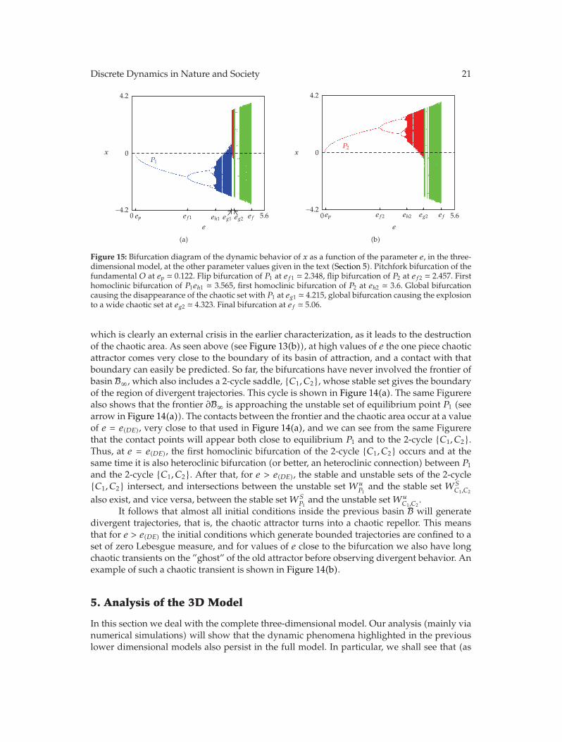
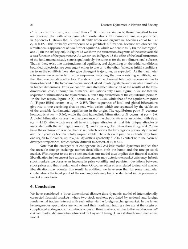
Figure 15: Bifurcation diagram of the dynamic behavior of x as a function of the parameter e, in the three-dimensional model, at the other parameter values given in the text (Section 5). Pitchfork bifurcation of thefundamental O at ep � 0.122. Flip bifurcation of P1 at ef1 � 2.348, flip bifurcation of P2 at ef2 � 2.457. Firsthomoclinic bifurcation of P1eh1 � 3.565, first homoclinic bifurcation of P2 at eh2 � 3.6. Global bifurcationcausing the disappearance of the chaotic set with P1 at eg1 � 4.215, global bifurcation causing the explosionto a wide chaotic set at eg2 � 4.323. Final bifurcation at ef � 5.06.

which is clearly an external crisis in the earlier characterization, as it leads to the destructionof the chaotic area. As seen above (see Figure 13(b)), at high values of e the one piece chaoticattractor comes very close to the boundary of its basin of attraction, and a contact with thatboundary can easily be predicted. So far, the bifurcations have never involved the frontier ofbasin B∞, which also includes a 2-cycle saddle, {C1, C2}, whose stable set gives the boundaryof the region of divergent trajectories. This cycle is shown in Figure 14(a). The same Figurerealso shows that the frontier ∂B∞ is approaching the unstable set of equilibrium point P1 (seearrow in Figure 14(a)). The contacts between the frontier and the chaotic area occur at a valueof e = e(DE), very close to that used in Figure 14(a), and we can see from the same Figurerethat the contact points will appear both close to equilibrium P1 and to the 2-cycle {C1, C2}.Thus, at e = e(DE), the first homoclinic bifurcation of the 2-cycle {C1, C2} occurs and at thesame time it is also heteroclinic bifurcation (or better, an heteroclinic connection) between P1

and the 2-cycle {C1, C2}. After that, for e > e(DE), the stable and unstable sets of the 2-cycle{C1, C2} intersect, and intersections between the unstable set Wu

P1and the stable set WS

C1,C2

also exist, and vice versa, between the stable set WSP1

and the unstable set WuC1,C2

.It follows that almost all initial conditions inside the previous basin B will generate

divergent trajectories, that is, the chaotic attractor turns into a chaotic repellor. This meansthat for e > e(DE) the initial conditions which generate bounded trajectories are confined to aset of zero Lebesgue measure, and for values of e close to the bifurcation we also have longchaotic transients on the ”ghost” of the old attractor before observing divergent behavior. Anexample of such a chaotic transient is shown in Figure 14(b).

5. Analysis of the 3D Model

In this section we deal with the complete three-dimensional model. Our analysis (mainly vianumerical simulations) will show that the dynamic phenomena highlighted in the previouslower dimensional models also persist in the full model. In particular, we shall see that (as


for the model in the previous section), the origin is always an equilibrium, and two moreequilibria appear as parameter e increases, leading to bistability. A sequence of local andglobal bifurcations then determine the transition between different dynamic regimes, namely,to more complex coexisting attractors, up to a global bifurcation which brings about a regimeof bull and bear market fluctuations, as we have seen both in the 1D and 2D model. Suchregime is characterized by apparently random switches of prices across different regions ofthe phase space (even more details on this setting may be found in Tramontana et al. [27]).

In the full model, stock market traders from countries A and H are allowed to trade inboth markets; that is, cH > 0 and cA > 0. In this case, the two stock prices and the exchangerate are all interdependent, and the model has the complete structure expressed by equations(2.1), (2.4), (2.7). The system, formulated in deviations (although we work with deviations, inall the following numerical experiments we have checked that original prices never becomenegative) from fundamental values, x = (PH − FH), y = (S − FS) and z = (PA − FA), isexpressed by the map T : R

3 → R3 in the following form:

T :

⎧⎪⎪⎪⎪⎪⎪⎪⎪⎪⎪⎪⎨⎪⎪⎪⎪⎪⎪⎪⎪⎪⎪⎪⎩

xt+1 = xt − aH[(bH + cH

)xt + cHγHyt

]

yt+1 = yt − d[cH(xt + FH

)(xt + γHyt

)]

−d[cA

zt + FA

yt + FS

(γA

yt

FS(yt + FS

) − zt)− eyt + fy3

t

]

zt+1 = zt − aA[(bA + cA

)zt − cAγA

yt

FS(yt + FS

)]

(5.1)

The model is analytically not tractable. Apart from the fundamental fixed point, say O =(0, 0, 0), whose existence can be immediately checked, we cannot solve explicitly forthe coordinates of further possible nonfundamental equilibria, nor can we obtain easilyinterpretable analytical conditions for their existence. A brief discussion of the steady statesis provided as follows.

By imposing the fixed point condition to (5.1), we obtain the following system ofequations:

(bH + cH

)x + cHγHy = 0, (5.2)

cH(x + FH

)(x + γHy

)+ cA

z + FA

y + FS

(γA

y

FS(y + FS

) − z)− ey + fy3 = 0, (5.3)

(bA + cA

)z − cAγA

y

FS(y + FS

) = 0. (5.4)

We observe from (5.2) and (5.4) that any steady state must belong to both the sets ofequations:

y = − x

qH, z = qA

y(y + FS

) , (5.5)


where

qH :=cHγH

bH + cH, qA :=

cAγA(bA + cA

)FS

(5.6)

This implies that when the steady state exchange rate is above the fundamental value (y > 0),steady state price A is then above the fundamental value (z > 0), whereas steady state priceH is below the fundamental value (x < 0), and vice versa. From now on, we will label theregion y > 0, z > 0, x < 0 as the bull region and region y < 0, z < 0, x > 0 as the bear region.

By substituting (5.5) into (5.3), we can express condition (5.3) in terms of the steadystate (deviation of) price H only, as follows:

x

[f

(qH)3x2 + bHx +

(bHFH − e

qH

)+M(x)

]= 0, (5.7)

where

M(x) := bAqHqAqHFSFA − x

(qA + FA

)(qHFS − x

)3. (5.8)

Therefore, besides the fundamental solution x = 0, further possible solutions are the rootsof the expression in square brackets in (5.7). When cA > 0 it becomes impossible to solveequation (5.7) analytically (as it was for cA = 0). When cA is small enough, we may expecta steady state structure qualitatively similar to that of the two-dimensional subcase cA = 0,with two further steady states appearing simultaneously in the bull region, via saddle-nodebifurcation, and this will be confirmed by the numerical example given below.

We remark that the analytical investigation of the local stability properties of thefundamental fixed point O = (0, 0, 0) is also a difficult task. The Jacobian matrix evaluatedat O is given by

J(O) :

⎡⎢⎢⎢⎢⎢⎢⎢⎣

1 − aH(bH + cH

)−aHcHγH 0

−dcHFH 1 − d[cHFHγH +

cAFAγA

(FS)3− e]

dcAFA

FS

0aAcAγA

(FS)2

1 − aA(bA + cA

)

⎤⎥⎥⎥⎥⎥⎥⎥⎦, (5.9)

and its eigenvalues cannot be found explicitly, nor can we write down tractable analyticalconditions for the eigenvalues to be smaller than one in modulus.

We will now study the local and global bifurcations via numerical investigation,supported by our knowledge of the model behavior in the simplified, two-dimensionalcase. Our base parameter selection is the following: aH = 0.41, bH = 0.11, cH = 0.83,FH = 4.279, γH = 0.3, d = 0.35, f = 0.7, FS = 6.07 (which are the same parameters usedin the previous section, enabling a direct comparison), aA = 0.43, bA = 0.21, cA = 0.2,γA = 0.36, and FA = 1.1. In order to compare the dynamics we have chosen a value of


cA not so far from zero, and lower than cH . Bifurcations similar to those described beloware observed also with other parameter constellations. The numerical analysis performedin Appendix D shows that O loses stability when one eigenvalue becomes equal to 1 atep � 0.122. This probably corresponds to a pitchfork bifurcation, because we observe thesimultaneous appearance of two further equilibria, which we denote as P1 (in the bear region)and P2 (in the bull region). In Figure 15 we show the bifurcation diagrams of the state variablex as a function of the parameter e. As we can see in Figure 15 the effect of the local bifurcationof the fundamental steady state is qualitatively the same as for the two-dimensional subcase.That is, there exist two nonfundamental equilibria, and depending on the initial conditions,bounded trajectories are convergent either to one or to the other (whereas initial conditionsfar from the equilibria here also give divergent trajectories, as expected). As the parametere increases we observe bifurcation sequences involving the two coexisting equilibria, andthen the two coexisting attractors. The structure of the observed bifurcations looks similar tothose observed in the two-dimensional model, albeit involving stable and unstable manifoldsin higher dimensions. Thus we confirm and strengthen almost all of the results of the two-dimensional case, although via numerical simulations only. From Figure 15 we see that thesequence of bifurcations are asynchronous, first a flip bifurcation of the equilibrium point P1

(in the bear region, Figure 15(a)) occurs, at ef1 � 2.348, while that of the equilibrium pointP2 (Figure 15(b)) occurs, at ef2 � 2.457. Then sequences of local and global bifurcationsgive rise to two coexisting chaotic sets, with basins which are separated by the stable setof the unstable fundamental equilibrium in the origin. The equilibrium point P1 becomeshomoclinic at eh1 � 3.565, while the first homoclinic bifurcation of P2 occurs, at eh2 � 3.6.A global bifurcation causes the disappearance of the chaotic attractor associated with P1 ateg1 � 4.215, after which we shall have a unique attractor. At first this unique attractor isassociated with the bull region around P2, and after a global bifurcation at eg2 � 4.323 wehave the explosion to a wide chaotic set, which covers the two regions previously disjoint,and the dynamics become totally unpredictable. The states will jump in a chaotic way fromone region to the other, up to a final bifurcation (probably due to a contact with the basin ofdivergent trajectories, which is now difficult to detect), at ef � 5.06.

Note that the emergence of endogenous bull and bear market dynamics implies thatthe unstable foreign exchange market destabilizes both the home and the foreign stockmarket. With respect to the two stock markets our model thus implies that financial marketliberalization in the sense of free capital movements may deteriorate market efficiency. In bothstock markets we observe an increase in price volatility and persistent deviations betweenstock prices and their fundamental values. Of course, other effects related to financial marketliberalization may counter this result. In addition, we have seen that for some parametercombinations the fixed point of the exchange rate may become stabilized in the presence ofmarket interactions.

6. Conclusion

We have considered a three-dimensional discrete-time dynamic model of internationallyconnected financial markets, where two stock markets, populated by national and foreignfundamental traders, interact with each other via the foreign exchange market. In the latter,heterogeneous speculators are active, and their nonlinear trading rules are at the origin ofcomplicated endogenous fluctuations across all three markets, similar to the well-known bulland bear market dynamics first observed by Day and Huang [1] in a stylized one-dimensionalmodel.


The possibility to reduce the dimension of the dynamical system, via restrictionsimposed on the activity of foreign traders, results in simplified one- and two-dimensionalsetups, whose analysis is simpler and helped in the understanding of those dynamicphenomena occurring in the complete three-dimensional model. While the one-dimensionalcase has the same qualitative dynamics of the Day and Huang [1] model, the two-dimensional model represents a generalization of such dynamics to the case of twointeracting markets, which can be studied by properly extending the methods and conceptsused in the one-dimensional analysis. These include, in particular, the properties ofnoninvertible maps and the theory of homoclinic bifurcations. The numerical and graphicalanalysis becomes essential when switching from the one- to the two-dimensional case.Nevertheless, a suitable mix of analytical and numerical techniques allows us to detect asequence of homoclinic bifurcations—analogous to those occurring in the one-dimensionalcase—through which the model switches across increasingly complex scenarios, as a crucialparameter is varied: from coexistence of two attractors in two distinct bull and bear areas,to the sudden disappearance of one of them, up to chaotic behavior on a unique attractor,with stock prices and exchange rates unpredictably switching among different regions of thephase space. Then we have seen that also in the three-dimensional model the local and globalbifurcations, when considered as a function of the same parameter, follow a path strictlyrelated to those of the two-dimensional model. From the coexistence of two attractors intwo distinct bull and bear areas we see a transition to a wide chaotic set in which the jumpsbetween the two regions become unpredictable.

Appendices

A.

In this appendix we compare the behavior, as the parameter e increases, of the maximumvalue xM0 (e) and that of the point α+(e) of the 2-cycle which bounds the basin of divergenttrajectories, showing that xM0 (e) increases faster than the point α+(e) so that the two valuesbecome equal at a finite value of the parameter e (called ef).

From (3.2) let us consider

xt+1 = φ(xt) = xt[A − Bx2

t

], A = (1 + de) , B = df. (A.1)

The second iterate of the map is given as

xt+2 = xt(A − Bx2

t

)[A − Bx2

t

(A2 +

(Bx2

t

)2− 2ABx2

t

)](A.2)

Let us now look at the solutions of the equation xt+2 = xt, among which are the periodic pointsof period-2 of the map φ. By defining ξ := Bx2

t we get a fourth-degree algebraic equation in ξ :

ξ4 − 3Aξ3 + 3A2ξ2 −(A +A3

)ξ +(A2 − 1

)= 0 (A.3)

whose roots are associated with the coordinates of the 2-cycle existing for x > 0, say ξ1 and ξ2,with the fixed point in the positive half-line (for which we know that the root is ξ∗ = A − 1)


and to the point ξ+ := B(α+)2. From the relations between the coefficients of the polynomial

and its roots we have

ξ1ξ2ξ∗ξ+ =

(A2 − 1

)(A.4)

so that

ξ1ξ2ξ+ = A + 1. (A.5)

We can thus conclude that the product ξ1ξ2ξ+ tends to∞ as fast as e, whereas we have xM0 (e) =2(1 + de)/3

√(1 + de)/3df , which tends to∞ as fast as e3/2.

B.

In this appendix we provide an analytical study of the eigenvalues of the Jacobian matrixevaluated at the fundamental steady state.

The Jacobian matrix of system (4.2) is the following:

J(x, y)

:

[1 − aH

(bH + cH

)−aHcHγH

−dcH(2x + γHy + FH

)1 − d

[cHγH

(x + FH

)− e + 3fy2]

], (B.1)

which, at the fundamental steady state O, becomes

J = J(0, 0) =

[1 − aH

(bH + cH

)−aHcHγH

−dcHFH 1 − d(cHγHFH − e

)]. (B.2)

The eigenvalues are the roots of the characteristic polynomial P(λ) = λ2 − tr(J)λ + det(J),where tr(J) and det(J) are the trace and determinant of J , respectively. Simple computationsallow us to check that [tr(J)]2 − 4det(J) > 0, which rules out the possibility of complexeigenvalues. In order to localize the (real) eigenvalues with respect to the interval [−1, 1], it isconvenient in this case to rewrite the characteristic equation in terms of the variable μ = 1−λ,as follows:

μ2 − αμ + β = 0, (B.3)

where

α = 2 − tr(J) =(bH + cH

)(aH + dqHFH

)− de, (B.4)

β = det(J) − tr(J) + 1 = daH(bH + cH

)(bHqHFH − e

), (B.5)


so that stability requires that both solutions of (B.3), say

μ1 :=α −√α2 − 4β

2, μ2 :=

α +√α2 − 4β

2, (B.6)

lie between 0 and 2. We simplify the analysis by introducing the additional requirement(which is largely fulfilled in our numerical examples) that parameters d and aH are not toolarge, namely,

(bH + cH

)(aH + dqHFH

)< 2. (B.7)

Note that this implies α < 2 for any d, e > 0, as can be checked. Let us now consider the effectof increasing parameter e. It is clear that for e < bHqHFH := eCS both α and β are also strictlypositive. Therefore, 0 < μ1 < μ2 < 2; that is, −1 < λ2 < λ1 < 1, where λ1 := 1 − μ1, λ2 := 1 − μ2.In particular, for e = bHqHFH , we obtain β = 0 and therefore 0 = μ1 < μ2 < 2. This meansthat λ1 = 1, while λ2 remains smaller than one in modulus. This corresponds to the loss ofstability of the fundamental steady state, through a transcritical bifurcation, as can be arguedfrom the numerical analysis performed in Section 4.

C.

In this appendix we provide the equation of the critical curve LC−1 of map T defined in (4.2).Starting from the Jacobian matrix (B.1), we can obtain LC−1, which is defined as the set ofpoints satisfying det(J(x, y)) = 0. This equation can be reduced to the following form:

x = Ay2 + By + C, (C.1)

where

A =−3f[1 − aH

(bH + cH

)]

cHγH[1 − aH

(bH + cH

)+ 2aHcH

] ,

B =−aHγHcH

1 − aH(bH + cH

)+ 2aHcH

,

C =

[1 − aH

(bH + cH

)][1 + d

(e − cHγHFH

)]

dcHγH[1 − aH

(bH + cH

)+ 2aHcH

] − aHcHFH

1 − aH(bH + cH

)+ 2aHcH

.

(C.2)

The image LC = T(LC−1) is a curve which separates the plane in regions whose points havea different number of rank-1 preimages. Here we have the case that any point has at leastone rank-1 preimage, while those on one side of curve LC have three rank-1 preimages. Thepoints belonging to curve LC have two merging rank-1 preimages in a point belonging toLC−1 and one more preimage (called extra preimage in Mira et al. [25]). An example of curvesLC−1 and LC is shown in Figure 9. As briefly explained in the text, such curves are responsiblefor the global bifurcations occurring to the structure of the basins of attractions. Disconnected


portions of the basins can only emerge in the case of noninvertible maps, and are associatedwith contacts of the basin boundary with curve LC (interested readers are invited to consultMira et al. [25]).

D.

Given the parameters selection used in this work (that is, aH = 0.41, bH = 0.11, cH = 0.83,FH = 4.279, γH = 0.3, d = 0.35, f = 0.7, FS = 6.07, aA = 0.43, bA = 0.21, cA = 0.2, γA =0.36, FA = 1.1), from (5.9) the Jacobian matrix of the three dimensional map evaluated at thefixed point O = (0, 0, 0) becomes

J(O) :

⎡⎢⎢⎣

0.6146 −0.10209 0

−1.2430495 0.626961205 + 0.35e 0.012685

0 0.00084 0.08237

⎤⎥⎥⎦ (D.1)

so that we look for the necessary and sufficient conditions for O to have all the eigenvaluesless than one in modulus, roots of the characteristic polynomial:

λ3 +A1λ2 +A2λ +A3 = 0, (D.2)

where

A1 = −2.0653 − 0.35e

A2 = 1.2811 + 0.503405e

A3 = −0.2129 − 0.1772e.

(D.3)

Following Farebrother [28] the eigenvalues of the polynomial given earlier have to satisfy thefollowing conditions (equivalent conditions can be found in Gandolfo [29], Yury’s conditionin Elaydi [30] and Okuguchi and Irie [31] :

(i) 1 +A1 +A2 +A3 > 0,

(ii) 1 −A1 +A2 −A3 > 0,

(iii) 1 −A2 +A1A3 − (A3)2 > 0,

(iv) A2 < 3.

In our case the condition (i) is satisfied if e < 0.122 (approximate value). Condition (ii)becomes 4.5593 + 1.0306e > 0 and is obviously satisfied for positive values of e. Condition(iii) is satisfied for e < 1.0738 and e > 3.445. The last condition is fulfilled for e < 3.4145.Starting from values of the parameter e positive and close to 0 and increasing the value, thefirst condition which is violated is (i), so e = 0.122 is the bifurcation value at which the fixedpoint loses stability, and at this value one eigenvalue is equal to 1.


References

[1] R. H. Day and W. Huang, “Bulls, bears and market sheep,” Journal of Economic Behavior andOrganization, vol. 14, no. 3, pp. 299–329, 1990.

[2] A. Kirman, “Epidemics of opinion and speculative bubbles in financial markets,” in Money andFinancial Markets, M. Taylor, Ed., pp. 354–368, Blackwell, Oxford, UK, 1991.

[3] C. Chiarella, “The dynamics of speculative behaviour,” Annals of Operations Research, vol. 37, no. 1–4,pp. 101–123, 1992.

[4] P. De Grauwe, H. Dewachter, and M. Embrechts, Exchange Rate Theory: Chaotic Models of ForeignExchange Markets, Blackwell, Oxford, UK, 1993.

[5] W. Huang and R. H. Day, “Chaotically switching bear and bull markets: the derivation of stock pricedistributions from behavioral rules,” in Non-Linear Dynamics and Evolutionary Economics, R. H. Dayand P. Chen, Eds., pp. 169–182, Oxford University Press, Oxford, UK, 1993.

[6] T. Lux, “Herd behavior, bubbles and crashes,” The Economic Journal, vol. 105, no. 431, pp. 881–896,1995.

[7] T. Lux, “The socio-economic dynamics of speculative markets: interacting agents, chaos, and the fattails of return distributions,” Journal of Economic Behavior and Organization, vol. 33, no. 2, pp. 143–165,1998.

[8] W. A. Brock and C. H. Hommes, “Heterogeneous beliefs and routes to chaos in a simple asset pricingmodel,” Journal of Economic Dynamics & Control, vol. 22, no. 8-9, pp. 1235–1274, 1998.

[9] C. Chiarella and X.-Z. He, “Asset price and wealth dynamics under heterogeneous expectations,”Quantitative Finance, vol. 1, no. 5, pp. 509–526, 2001.

[10] C. Chiarella and X.-Z. He, “Heterogeneous beliefs, risk and learning in a simple asset pricing modelwith a market maker,” Macroeconomic Dynamics, vol. 7, no. 4, pp. 503–536, 2003.

[11] J. D. Farmer and S. Joshi, “The price dynamics of common trading strategies,” Journal of EconomicBehavior and Organization, vol. 49, no. 2, pp. 149–171, 2002.

[12] C. Chiarella, R. Dieci, and L. Gardini, “Speculative behaviour and complex asset price dynamics: aglobal analysis,” Journal of Economic Behavior and Organization, vol. 49, no. 2, pp. 173–197, 2002.

[13] C. Hommes, H. Huang, and D. Wang, “A robust rational route to randomness in a simple asset pricingmodel,” Journal of Economic Dynamics & Control, vol. 29, no. 6, pp. 1043–1072, 2005.

[14] C. Hommes, “Heterogeneous agent models in economics and finance,” in Handbook of ComputationalEconomics Vol. 2: Agent-Based Computational Economics, L. Tesfatsion and K. Judd, Eds., North-Holland,Amsterdam, The Netherlands, 2006.

[15] B. LeBaron, “Agent-based computational finance,” in Handbook of Computational Economics Vol. 2:Agent-Based Computational Economics, L. Tesfatsion and K. Judd, Eds., pp. 1187–1233, North-Holland,Amsterdam, The Netherlands, 2006.

[16] T. Lux, “Financial power laws: empirical evidence, models and mechanisms,” in Power Laws in theSocial Sciences: Discovering Complexity and Non-Equilibrium Dynamics in the Social Universe, C. Cioffi-Revilla, Ed., Cambridge University Press, Cambridge, UK, 2008.

[17] F. Westerhoff, “Exchange rate dynamics: a nonlinear survey,” in Handbook of Research on Complexity, J.B. Rosser, Ed., Edward Elgar, Cheltenham, UK, 2009.

[18] C. Chiarella, R. Dieci, and X.-Z. He, “Heterogeneity, market mechanisms and asset price dynamics,”in Handbook of Financial Markets: Dynamics and Evolution, T. Hens and K. R. Schenk-Hoppe, Eds., pp.277–344, North Holland, Amsterdam, The Netherlands, 2009.

[19] F. Westerhoff, “Multiasset market dynamics,” Macroeconomic Dynamics, vol. 8, no. 5, pp. 596–616, 2004.[20] C. Chiarella, R. Dieci, and L. Gardini, “The dynamic interaction of speculation and diversification,”

Applied Mathematical Finance, vol. 12, no. 1, pp. 17–52, 2005.[21] F. H. Westerhoff and R. Dieci, “The effectiveness of Keynes-Tobin transaction taxes when

heterogeneous agents can trade in different markets: a behavioral finance approach,” Journal ofEconomic Dynamics & Control, vol. 30, no. 2, pp. 293–322, 2006.

[22] R. Dieci and F. Westerhoff, “Heterogeneous speculators, endogenous fluctuations and interactingmarkets: a model of stock prices and exchange rates,” Working paper, University of Bologna, Bologna,Italy, 2008.

[23] R. Dieci, G.-I. Bischi, and L. Gardini, “From bi-stability to chaotic oscillations in a macroeconomicmodel,” Chaos, Solitons & Fractals, vol. 12, no. 5, pp. 805–822, 2001.


[24] X.-Z. He and F. H. Westerhoff, “Commodity markets, price limiters and speculative price dynamics,”Journal of Economic Dynamics & Control, vol. 29, no. 9, pp. 1577–1596, 2005.

[25] C. Mira, L. Gardini, A. Barugola, and J.-C. Cathala, Chaotic Dynamics in Two-Dimensional NoninvertibleMaps, vol. 20 of World Scientific Series on Nonlinear Science. Series A: Monographs and Treatises, WorldScientific, River Edge, NJ, USA, 1996.

[26] C. Grebogi, E. Ott, and J. A. Yorke, “Crises, sudden changes in chaotic attractors, and transient chaos,”Physica D, vol. 7, no. 1–3, pp. 181–200, 1983.

[27] F. Tramontana, L. Gardini, R. Dieci, and F. Westerhoff, “The emergence of “bull and bear” dynamicsin a nonlinear model of interacting markets,” in Nonlinear Dynamics in Economics, Finance and SocialSciences, C. Chiarella, G. I. Bischi, and L. Gardini, Eds., Springer, New York, NY, USA, 2009.

[28] R. W. Farebrother, “Simplified Samuelson conditions for cubit and quartic equations,” The ManchesterSchool of Econonomics and Social Studies, vol. 41, no. 4, pp. 396–400, 1973.

[29] G. Gandolfo, Economic Dynamics: Methods and Models, vol. 16 of Advanced Textbooks in Economics,North-Holland, Amsterdam, The Netherlands, 2nd edition, 1980.

[30] S. N. Elaydi, An Introduction to Difference Equations, Springer, New York, NY, USA, 1995.[31] K. Okuguchi and K. Irie, “The Shur and Samuelson conditions for a cubic equation,” The Manchester

School of Econonomics and Social Studies, vol. 58, no. 4, pp. 414–418, 1990.

The Emergence of Bull and Bear Dynamics in a Nonlinear Model of Interacting Markets

Documents

Transcript of The Emergence of Bull and Bear Dynamics in a Nonlinear Model of Interacting Markets