Most probable histories for nonlinear dynamics: tracking climate transitions
V12N3.pdf - Nonlinear Dynamics and Systems Theory
114
NONLINEAR DYNAMICS AND SYSTEMS THEORY Volume Number 20 CONTENTS 12 3 12 An International Journal of Research and Surveys © 20 , Infor ath Publishing Group ISSN 1562-8353 Printed in Ukraine To receive contents by e-mail, visit our Website at: 12 M and abstracts http://www.e-ndst.kiev.ua Nonlinear Dynamics and Systems Theory An International Journal of Research and Surveys Volume , Number , 20 ISSN 1562-8353 12 3 12 NONLINEAR DYNAMICS & SYSTEMS THEORY Volume , No. , 20 12 3 12 EDITOR-IN-CHIEF A.A.MARTYNYUK REGIONAL EDITORS P.BORNE, Lille, France C.CORDUNEANU, Arlington, TX, USA , , PENG SHI, Pontypridd, United Kingdom K.L.TEO, H.I.FREEDMAN, Edmonton, Canada S.P.Timoshenko Institute of Mechanics National Academy of Sciences of Ukraine, Kiev, Ukraine Europe USA, Central and South America Australia New Zealand Canada China and South East Asia and North America and Ensenada Mexico Perth, Australia C.CRUZ-HERNANDEZ InforMath Publishing Group http://www.e-ndst.kiev.ua Numerical Solutions of System of Non-linear ODEs by Euler Modified Method .......................................................................................... 215 B. S. Desale and N. R. Dasre Euler Solutions for Integro Differential Equations with Retardation and Anticipation ............................................................................................ 237 J. Vasundhara Devi and Ch.V. Sreedhar Representation of the Solution for Linear System of Delay Equations with Distributed Parameters ......................................................... 251 J. Diblik, D. Khusainov and O. Kukharenko Partial Control Design for Nonlinear Control Systems ................................ 269 M.H. Shafiei and T. Binazadeh Wavelet Neural Network Based Adaptive Tracking Control for a Class of Uncertain Nonlinear Systems Using Reinforcement Learning ....... 279 M. Sharma and A. Verma Sum of Linear Ratios Multiobjective Programming Problem: A Fuzzy Goal Programming Approach ........................................................ 289 Pitam Singh and D. Dutta Approximate Controllability of Nonlocal Semilinear Time-varying Delay Control Systems ................................................................................. 303 N.K. Tomar and S. Kumar Existence of Positive Solutions of a Nonlinear Third-Order M-Point Boundary Value Problem for p-Laplacian Dynamic Equations on Time Scales .............................................................................................. 311 N. Yolcu and S. Topal
-
Upload
khangminh22 -
Category
Documents
-
view
3 -
download
0
Transcript of V12N3.pdf - Nonlinear Dynamics and Systems Theory
NONLINEAR DYNAMICS AND SYSTEMS THEORY
Volume Number 20
CONTENTS
12 3 12
An International Journal of Research and Surveys
© 20 , Infor ath Publishing Group ISSN 1562-8353 Printed in UkraineTo receive contents by e-mail, visit our Website at:
12 Mand abstracts http://www.e-ndst.kiev.ua
Nonlinear Dynamics
and
Systems Theory
An International Journal of Research and Surveys
Volume , Number , 20 ISSN 1562-835312 3 12
NO
NLIN
EA
R D
YN
AM
ICS &
SYSTE
MS TH
EO
RY
Vo
lum
e , N
o. , 2
01
23
12
EDITOR-IN-CHIEF A.A.MARTYNYUK
REGIONAL EDITORS
P.BORNE, Lille, France
C.CORDUNEANU, Arlington, TX, USA, ,
PENG SHI, Pontypridd, United Kingdom
K.L.TEO,
H.I.FREEDMAN, Edmonton, Canada
S.P.Timoshenko Institute of MechanicsNational Academy of Sciences of Ukraine, Kiev, Ukraine
Europe
USA, Central and South America
Australia New Zealand
Canada
China and South East Asia
and
North America and
Ensenada Mexico
Perth, Australia
C.CRUZ-HERNANDEZ
InforMath Publishing Grouphttp://www.e-ndst.kiev.ua
Numerical Solutions of System of Non-linear ODEs by Euler
Modified Method .......................................................................................... 215B. S. Desale and N. R. Dasre
Euler Solutions for Integro Differential Equations with Retardationand Anticipation ............................................................................................ 237
J. Vasundhara Devi and Ch.V. Sreedhar
Representation of the Solution for Linear System of DelayEquations with Distributed Parameters ......................................................... 251
J. Diblik, D. Khusainov and O. Kukharenko
Partial Control Design for Nonlinear Control Systems ................................ 269M.H. Shafiei and T. Binazadeh
Wavelet Neural Network Based Adaptive Tracking Control for aClass of Uncertain Nonlinear Systems Using Reinforcement Learning ....... 279
M. Sharma and A. Verma
Sum of Linear Ratios Multiobjective Programming Problem:A Fuzzy Goal Programming Approach ........................................................ 289
Pitam Singh and D. Dutta
Approximate Controllability of Nonlocal Semilinear Time-varyingDelay Control Systems ................................................................................. 303
N.K. Tomar and S. Kumar
Existence of Positive Solutions of a Nonlinear Third-Order M-PointBoundary Value Problem for p-Laplacian Dynamic Equations
on Time Scales .............................................................................................. 311N. Yolcu and S. Topal
(1) General. Nonlinear Dynamics and Systems Theory (ND&ST) is an international journal
devoted to publishing peer-refereed, high quality, original papers, brief notes and reviewarticles focusing on nonlinear dynamics and systems theory and their practical applications in
engineering, physical and life sciences. Submission of a manuscript is a representation that thesubmission has been approved by all of the authors and by the institution where the work was
carried out. It also represents that the manuscript has not been previously published, has notbeen copyrighted, is not being submitted for publication elsewhere, and that the authors have
agreed that the copyright in the article shall be assigned exclusively to InforMath PublishingGroup by signing a transfer of copyright form. Before submission, the authors should visit the
website:http://www.e-ndst.kiev.ua
for information on the preparation of accepted manuscripts. Please download the archive
Sample_NDST.zip containing example of article file (you can edit only the fileSamplefilename.tex).
(2) Manuscript and Correspondence. Manuscripts should be in English and must meetcommon standards of usage and grammar. To submit a paper, send by e-mail a file in PDF
format directly toProfessor A.A. Martynyuk, Institute of Mechanics,
Nesterov str.3, 03057, MSP 680, Kiev-57, Ukrainee-mail: [email protected]; [email protected]
or to one of the Regional Editors or to a member of the Editorial Board. Final version of themanuscript must typeset using LaTex program which is prepared in accordance with the style
file of the Journal. Manuscript texts should contain the title of the article, name(s) of theauthor(s) and complete affiliations. Each article requires an abstract not exceeding 150 words.
Formulas and citations should not be included in the abstract. AMS subject classifications andkey words must be included in all accepted papers. Each article requires a running head
(abbreviated form of the title) of no more than 30 characters. The sizes for regular papers,survey articles, brief notes, letters to editors and book reviews are: (i) 10-14 pages for regular
papers, (ii) up to 24 pages for survey articles, and (iii) 2-3 pages for brief notes, letters to theeditor and book reviews.
(3) Tables, Graphs and Illustrations. Each figure must be of a quality suitable for directreproduction and must include a caption. Drawings should include all relevant details and
should be drawn professionally in black ink on plain white drawing paper. In addition to ahard copy of the artwork, it is necessary to attach the electronic file of the artwork (preferably
in PCX format).(4) References. References should be listed alphabetically and numbered, typed andpunctuated according to the following examples. Each entry must be cited in the text in form
of author(s) together with the number of the referred article or in the form of the number ofthe referred article alone.
Journal: [1] Poincare, H. Title of the article. Title of the Journal Vol. l(No.l), Year, Pages. [Language]
Book: [2] Liapunov, A.M. Title of the book. Name of the Publishers,Town, Year.
Proceeding: [3] Bellman, R. Title of the article. In: Title of the book. (Eds.).Name of the Publishers, Town, Year, Pages. [Language]
(5) Proofs and Sample Copy. Proofs sent to authors should be returned to the EditorialOffice with corrections within three days after receipt. The corresponding author will receive
a sample copy of the issue of the Journal for which his/her paper is published.(6) Editorial Policy. Every submission will undergo a stringent peer review process. An
editor will be assigned to handle the review process of the paper. He/she will secure at leasttwo reviewers’ reports. The decision on acceptance, rejection or acceptance subject to revision
will be made based on these reviewers’ reports and the editor’s own reading of the paper.
INSTRUCTIONS FOR CONTRIBUTORSNonlinear Dynamics and Systems TheoryAn International Journal of Research and Surveys
EDITOR .
HONORARY EDITORS
MANAGING EDITOR
REGIONAL EDITORS
EDITORIAL BOARD
-IN-CHIEF A A.MARTYNYUK
, , , USA
I.P.STAVROULAKIS
P.BORNE (France), e-mail: [email protected] (USA), e-mail: co @uta.edu
C. ( ), e-mail:P.SHI (United Kingdom), e-mail: [email protected]
K.L.TEO ( ), e-mail: eo@(Canada), e-mail: [email protected]
The S.P.Timoshenko Institute of Mechanics, National Academy of Sciences of Ukraine,Nesterov Str. 3, 03680 MSP, Kiev-57, UKRAINE / e-mail: [email protected]
e-mail: [email protected]
/Department of Mathematics, University of Ioannina
451 10 Ioannina, HELLAS (GREECE) e-mail: [email protected]
T.A.BURTON Port Angeles WAS.N.VASSILYEV
ncordCRUZ-HERNANDEZ Mexico [email protected]
Australia K.L.T curtin.edu.auH.I.FREEDMAN
, ,Moscow Russia
Artstein, Z. (Israel)
Bohner, M. (USA), . . ( )
Ch -H (USA)Chen Ye-Hwa (USA)D'Anna, A. (Italy)Dauphin-Tanguy, G. (France)Dshalalow, J.H. (USA)Eke, F.O. (USA)
Fabrizio, M. (Italy)Georgiou, G. (Cyprus)Guang-Ren Duan (China)Izobov, N.A. (Belarussia)
Khusainov, D.Ya. (Ukraine)
Bajodah, A.H. (Saudi Arabia)
Braiek N B Tunisiaang M. .
Enciso, G. (USA)
Kalauch, A. (Germany)Karimi, H.R. (Norway)
Kloeden, P. (Germany)
Leonov, G.A. (Russia)Limarchenko, O.S. (Ukraine)Loccufier, M. (Belgium)
Nguang Sing Kiong (New Zealand)
Shi Yan (Japan)Siljak, D.D. (USA)
Sree Hari Rao, V. (India)Stavrakakis, N.M. (Greece)
Vatsala, A. (USA)
Wuyi Yue (Japan)
Kokologiannaki, C. (Greece)Lazar, M. (The Netherlands)
Lopes-Gutieres, R.M. (Mexico)
Rasmussen, M. (United Kingdom)
Sira-Ramirez, H. (Mexico)
Sun Xi-Ming (China)
Wang Hao (Canada)
© 20 , Infor ath Publishing Group SSN 1562-8353 Printed in UkraineNo part of this Journal may be reproduced or transmitted in any form or by any means withoutpermission from Infor ath Publishing Group.
12 M , I print, ISSN 1813-7385 online,
M
ADVISORY EDITOR
ADVISORY COMPUTER SCIENCE EDITOR
ADVISORY EDITOR
A. . KO, Kiev, Ukraine
A.N.CHERNIENKO L.N.CHERNETSKAYA, Kiev, Ukraine
S.N.RASSH VALOVA, Kiev, Ukraine
G MAZe-mail: [email protected]
and
Y
S
LINGUISTIC
NONLINEAR DYNAMICS AND SYSTEMS THEORY
An International Journal of Research and Surveys
Published by InforMath Publishing Group since 2001
Volume 12 Number 3 2012
CONTENTS
Numerical Solutions of System of Non-linear ODEs by Euler
Modified Method . . . . . . . . . . . . . . . . . . . . . . . . . . . . . . . . . . . . . . . . . . . . . . . . . . . . 215
B. S. Desale and N. R. Dasre
Euler Solutions for Integro Differential Equations with Retardation
and Anticipation . . . . . . . . . . . . . . . . . . . . . . . . . . . . . . . . . . . . . . . . . . . . . . . . . . . . 237
J. Vasundhara Devi and Ch.V. Sreedhar
Representation of the Solution for Linear System of Delay
Equations with Distributed Parameters . . . . . . . . . . . . . . . . . . . . . . . . . . . . . . 251
J. Diblik, D. Khusainov and O. Kukharenko
Partial Control Design for Nonlinear Control Systems . . . . . . . . . . . . . . . . 269
M.H. Shafiei and T. Binazadeh
Wavelet Neural Network Based Adaptive Tracking Control for a
Class of Uncertain Nonlinear Systems Using Reinforcement Learning . 279
M. Sharma and A. Verma
Sum of Linear Ratios Multiobjective Programming Problem:
A Fuzzy Goal Programming Approach . . . . . . . . . . . . . . . . . . . . . . . . . . . . . . . 289
Pitam Singh and D. Dutta
Approximate Controllability of Nonlocal Semilinear Time-varying
Delay Control Systems . . . . . . . . . . . . . . . . . . . . . . . . . . . . . . . . . . . . . . . . . . . . . . . 303
N.K. Tomar and S. Kumar
Existence of Positive Solutions of a Nonlinear Third-Order M-Point
Boundary Value Problem for p-Laplacian Dynamic Equations
on Time Scales . . . . . . . . . . . . . . . . . . . . . . . . . . . . . . . . . . . . . . . . . . . . . . . . . . . . . . 311
N. Yolcu and S. Topal
Founded by A.A. Martynyuk in 2001.
Registered in Ukraine Number: KB 5267 / 04.07.2001.
NONLINEAR DYNAMICS AND SYSTEMS THEORY
An International Journal of Research and Surveys
Nonlinear Dynamics and Systems Theory (ISSN 1562–8353 (Print), ISSN 1813–7385 (Online)) is an international journal published under the auspices of the S.P. Timo-shenko Institute of Mechanics of National Academy of Sciences of Ukraine and CurtinUniversity of Technology (Perth, Australia). It aims to publish high quality originalscientific papers and surveys in areas of nonlinear dynamics and systems theory andtheir real world applications.
AIMS AND SCOPE
Nonlinear Dynamics and Systems Theory is a multidisciplinary journal. It pub-lishes papers focusing on proofs of important theorems as well as papers presenting newideas and new theory, conjectures, numerical algorithms and physical experiments inareas related to nonlinear dynamics and systems theory. Papers that deal with theo-retical aspects of nonlinear dynamics and/or systems theory should contain significantmathematical results with an indication of their possible applications. Papers that em-phasize applications should contain new mathematical models of real world phenomenaand/or description of engineering problems. They should include rigorous analysis ofdata used and results obtained. Papers that integrate and interrelate ideas and methodsof nonlinear dynamics and systems theory will be particularly welcomed. This journaland the individual contributions published therein are protected under the copyright byInternational InforMath Publishing Group.
PUBLICATION AND SUBSCRIPTION INFORMATION
Nonlinear Dynamics and Systems Theory will have 4 issues in 2012,printed in hard copy (ISSN 1562–8353) and available online (ISSN 1813–7385),by InforMath Publishing Group, Nesterov str., 3, Institute of Mechanics, Kiev,MSP 680, Ukraine, 03057. Subscription prices are available upon request fromthe Publisher (mailto:[email protected]), SWETS Information ServicesB.V. (mailto:[email protected]), EBSCO Information Services(mailto:[email protected]), or website of the Journal: http://e-ndst.kiev.ua.Subscriptions are accepted on a calendar year basis. Issues are sent by airmail to allcountries of the world. Claims for missing issues should be made within six months ofthe date of dispatch.
ABSTRACTING AND INDEXING SERVICES
Papers published in this journal are indexed or abstracted in: Mathematical Reviews /MathSciNet, Zentralblatt MATH / Mathematics Abstracts, PASCAL database (INIST–CNRS) and SCOPUS.
Nonlinear Dynamics and Systems Theory, 12 (3) (2012) 215–236
Numerical Solutions of System of Non-linear ODEs by
Euler Modified Method
B. S. Desale ∗ and N. R. Dasre
School of Mathematical Sciences, North Maharashtra University,
Jalgaon 425001, India
Received: June 29, 2011; Revised: June 19, 2012
Abstract: In this paper, we have proposed Euler’s modified method for solving thesix coupled system of non-linear ordinary differential equations (ODEs), which arearoused in the reduction of stratified Boussinesq equations. This method can also becalled as revised Euler’s modified method for solving two simultaneous ODEs. Wehave obtained the numerical solutions on stable and unstable manifolds. The errorbetween the numerical solution and exact solution is of order 10−20 to 10−6. We havecoded this programme in C-language.
Keywords: stratified Boussinesq equation, Euler modified method, integrable
systems.
Mathematics Subject Classification (2010): 34A09, 65L05, 65L99.
1 Introduction
The stratified Boussinesq equations form a system of Partial Differential Equations(PDEs) modelling the movements of planetary atmospheres. It may be noted that liter-ature also refers to Boussinesq approximation as Oberbeck–Boussinesq approximation.For this, one may refer to an interesting article by Rajagopal et al [1] which providesa rigorous mathematical justification for perturbations of the Navier-Stokes equations.Majda & Shefter [2] have chosen certain special solutions of this system of ODEs todemonstrate the onset of instability when the Richardson number is less than 1/4. Ma-jda and Shefter [3] have shown that the analysis, in the special cases considered, reducesto the solutions of Hamiltonian system. These reductions form an interesting coupledsystem of six non-linear ODEs. Shrinivasan et al [4] have also tested the system for com-plete integrability by use of first integrals. Further, Desale [6] has incorporated the effect
∗ Corresponding author: mailto:[email protected]
c© 2012 InforMath Publishing Group/1562-8353 (print)/1813-7385 (online)/http://e-ndst.kiev.ua215
216 B.S. DESALE AND N.R. DASRE
of rotation in the same system in the context of basin scale dynamics, while Desale andSharma [7] have given special solutions of rotating stratified Boussinesq equations. De-sale and Patil [8] have tested the system of six coupled nonlinear ODEs by Painleve Test.Burton and Zhang [9] have given the periodic solutions for singular integral equations.Biswas et al [10] have studied the behavior of soliton solutions in the form of KdV partialdifferential equation in the fiber optics solitons theory in communication engineering.
In this paper, we have given the C-code to find and to test the initial values whichlie on the invariant surface given by equation (4). We have implemented Euler Modifiedmethod to find the numerical solution of the system (1) passing through the initial valueson invariant surface (4). We have discussed the use of this method in the subsection (3.1).We have given the codes for solutions on stable and unstable manifolds of invariant surfacewhich is obtained by four first integrals.
2 Preliminaries
Shrinivasan et al [4] have tested the system (1) as given below for complete integrability.Also, Deasle and Shrinivasan [5] have shown that in the general case, the problem ofintegration reduces to the integrations of the system of six coupled autonomous ODE’s
w = gρb
e3 × b,
b = 12w × b,
(1)
wherew = (w1, w2, w3)T , b = (b1, b2, b3)
T and gρb
is a non-dimensional constant as men-
tioned by Desale [11] in his Ph. D. thesis.The above system can be written component-wise as below
w1 = − gρb
b2, w2 = gρb
b1, w1 = 0,
b1 = 12 (w2b3 − w3b2), b2 = 1
2 (w3b1 − w1b3), b3 =12 (w1b2 − w2b1).
(2)
The system (1) admits the following four first integrals
1) |b|2 = c1,
2) w · b = c2,
3) e3 ·w = c3,
4) |w|22 + 2g
ρb
e3 · b = c4,
(3)
with non zero values of c1, c2, c3 and c4. The possible critical points of the system (1)are (±e3,±e3). For c1 = 1 and w = ±e3, c3 may assume the values ±1 (not both).Now we take c3 = 1, so that the possible critical points are (e3,±e3). At the rest points(e3,±e3), the value of c2 is ±1.
Remark 2.1 The case c2 = −1 will be surface disjoint from w ·b = 1 and the similaranalysis will be carried out if we take c2 = −1. Right now we take c1 = 1, c2 = 1 andc3 = 1. But this forces b = e3 at a critical point, so with our specific conditions we haveonly one rest point (e3, e3) on the invariant surface (3). At this critical point fourth firstintegral assumes the value c4 = 1
2 + 2gρb
.
NONLINEAR DYNAMICS AND SYSTEMS THEORY, 12 (3) (2012) 215–236 217
With the above specification, we have following four first integrals
|b|2 = 1,w · b = 1, e3 ·w = 1,|w|22
+2g
ρbe3 · b =
1
2+
2g
ρb. (4)
A critical point (e3, e3) lies on invariant surface and (b1, b2, b3) is on the surface|b|2 = 1. Therefore we have
w1 =−b2k
1− b3+
b11 + b3
,
w2 =b1k
1− b3+
b21 + b3
,
w3 = 1.
(5)
where k is a function of b3, given by the following equation
k2 =(1− b3)
2
(1 + b3)2
[4g(1 + b3)− ρbρb
]
. (6)
One may refer [4, 5] for more details of this analysis. Since |b|2 = 1, we can usespherical-polar co-ordinates
b1 = cos θ sinφ, b2 = sin θ sinφ, b3 = cosφ. (7)
Hence,
k2 = tan4(φ
2)[8g
ρbcos2(
φ
2)− 1
]
. (8)
For k to be real , Shrinivasan et al [5] have put up the restriction to φ as 0 ≤ φ ≤2 cos−1(
√
ρb
8g ). With this limitation k takes the values negative, positive and zero. With
these possible choices of k, the invariant surface will be the union of disjoint manifoldscorresponding to k > 0, is unstable manifold, k < 0, is stable manifold and k = 0, is acenter manifold. Regarding these manifolds, readers are advised to refer to Shrinivasanet al [5].
Now for k > 0, the unstable manifold is given by
w1 = tan(φ2 )[
cos θ − sin θ√
8gρb
cos2(φ2 )− 1]
,
w2 = tan(φ2 )[
cos θ + sin θ√
8gρb
cos2(φ2 )− 1]
,
w3 = 1,
b1 = cos θ sinφ,
b2 = sin θ sinφ,
b3 = cosφ,
with
k = tan2(φ
2)[8g
ρbcos2(
φ
2)− 1
]
.
(9)
218 B.S. DESALE AND N.R. DASRE
On this surface, system (1) reduces to
dφ
dt= 1
2 tan(φ2 )√
8gρb
cos2(φ2 )− 1,
dθ
dt= 1
4 sec2(φ2 ),
(10)
where as for k < 0, the stable manifold is given by
w1 = tan(φ2 )[
cos θ + sin θ√
8gρb
cos2(φ2 )− 1]
,
w2 = tan(φ2 )[
cos θ − sin θ√
8gρb
cos2(φ2 )− 1]
,
w3 = 1,
b1 = cos θ sinφ,
b2 = sin θ sinφ,
b3 = cosφ,
with
k = − tan2(φ2 )[
8gρb
cos2(φ2 )− 1]
.
(11)
On this surface, system (1) reduces to
dφ
dt= − 1
2 tan(φ2 )√
8gρb
cos2(φ2 )− 1,
dθ
dt= 1
4 sec2(φ2 ).
(12)
3 Numerical Solution
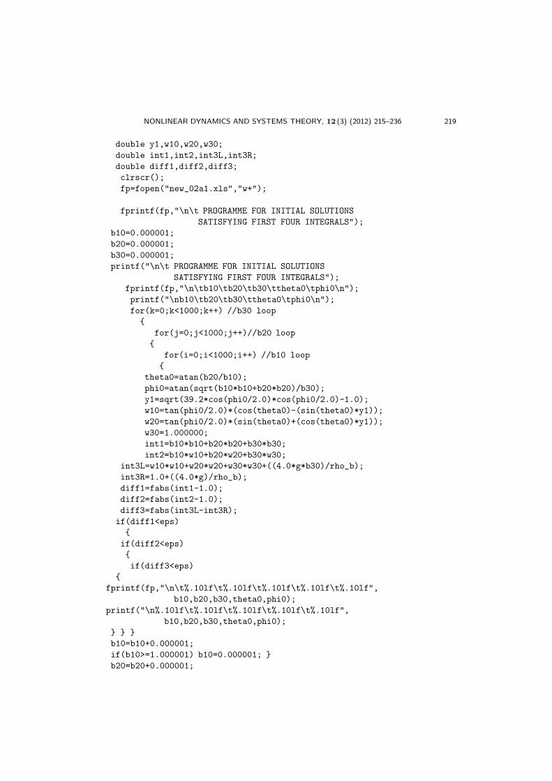
In their studies, Shrinivasan et al [5] have shown that the system (1) is completelyintegrable and solutions exist on invariant surface (3) for all the time. So we are lookingfor the numerical solution of the system (1) on the invariant surface (3). We find theinitial values which satisfy the four first integrals given by (4) and consequently we canfind the solutions of system (1) passing through these initial values. We use the followingprogramme to find the initial values so that they satisfy the four first integrals. We usethe following programme to test finitely many points.
#include<stdio.h>
#include<conio.h>
#include<math.h>
void main()
FILE *fp;
double b10,b20,b30,phi0,theta0;
double eps=0.0000001,G=39.2;
double g=9.8,rho_b=2;
long int i,j,k;
NONLINEAR DYNAMICS AND SYSTEMS THEORY, 12 (3) (2012) 215–236 219
double y1,w10,w20,w30;
double int1,int2,int3L,int3R;
double diff1,diff2,diff3;
clrscr();
fp=fopen("new_02a1.xls","w+");
fprintf(fp,"\n\t PROGRAMME FOR INITIAL SOLUTIONS
SATISFYING FIRST FOUR INTEGRALS");
b10=0.000001;
b20=0.000001;
b30=0.000001;
printf("\n\t PROGRAMME FOR INITIAL SOLUTIONS
SATISFYING FIRST FOUR INTEGRALS");
fprintf(fp,"\n\tb10\tb20\tb30\ttheta0\tphi0\n");
printf("\nb10\tb20\tb30\ttheta0\tphi0\n");
for(k=0;k<1000;k++) //b30 loop
for(j=0;j<1000;j++)//b20 loop
for(i=0;i<1000;i++) //b10 loop
theta0=atan(b20/b10);
phi0=atan(sqrt(b10*b10+b20*b20)/b30);
y1=sqrt(39.2*cos(phi0/2.0)*cos(phi0/2.0)-1.0);
w10=tan(phi0/2.0)*(cos(theta0)-(sin(theta0)*y1));
w20=tan(phi0/2.0)*(sin(theta0)+(cos(theta0)*y1));
w30=1.000000;
int1=b10*b10+b20*b20+b30*b30;
int2=b10*w10+b20*w20+b30*w30;
int3L=w10*w10+w20*w20+w30*w30+((4.0*g*b30)/rho_b);
int3R=1.0+((4.0*g)/rho_b);
diff1=fabs(int1-1.0);
diff2=fabs(int2-1.0);
diff3=fabs(int3L-int3R);
if(diff1<eps)
if(diff2<eps)
if(diff3<eps)
fprintf(fp,"\n\t%.10lf\t%.10lf\t%.10lf\t%.10lf\t%.10lf",
b10,b20,b30,theta0,phi0);
printf("\n%.10lf\t%.10lf\t%.10lf\t%.10lf\t%.10lf",
b10,b20,b30,theta0,phi0);
b10=b10+0.000001;
if(b10>=1.000001) b10=0.000001;
b20=b20+0.000001;
220 B.S. DESALE AND N.R. DASRE
if(b20>=1.000001) b20=0.000001;
b30=b30+0.000001;
if(b30>=1.000001) b30=0.000001;
getch();
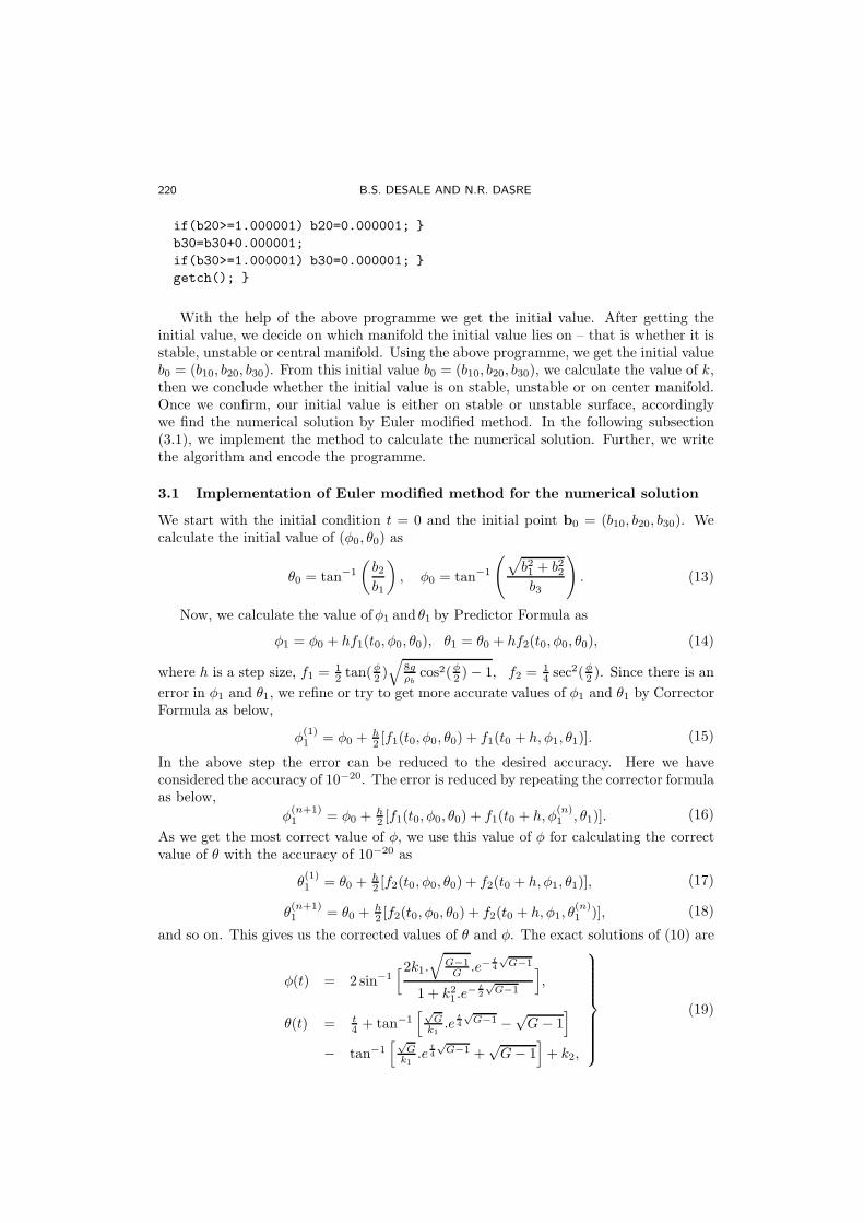
With the help of the above programme we get the initial value. After getting theinitial value, we decide on which manifold the initial value lies on – that is whether it isstable, unstable or central manifold. Using the above programme, we get the initial valueb0 = (b10, b20, b30). From this initial value b0 = (b10, b20, b30), we calculate the value of k,then we conclude whether the initial value is on stable, unstable or on center manifold.Once we confirm, our initial value is either on stable or unstable surface, accordinglywe find the numerical solution by Euler modified method. In the following subsection(3.1), we implement the method to calculate the numerical solution. Further, we writethe algorithm and encode the programme.
3.1 Implementation of Euler modified method for the numerical solution
We start with the initial condition t = 0 and the initial point b0 = (b10, b20, b30). Wecalculate the initial value of (φ0, θ0) as
θ0 = tan−1
(
b2b1
)
, φ0 = tan−1
(
√
b21 + b22b3
)
. (13)
Now, we calculate the value ofφ1 and θ1 by Predictor Formula as
φ1 = φ0 + hf1(t0, φ0, θ0), θ1 = θ0 + hf2(t0, φ0, θ0), (14)
where h is a step size, f1 = 12 tan(
φ2 )√
8gρb
cos2(φ2 )− 1, f2 = 14 sec
2(φ2 ). Since there is an
error in φ1 and θ1, we refine or try to get more accurate values of φ1 and θ1 by CorrectorFormula as below,
φ(1)1 = φ0 +
h2 [f1(t0, φ0, θ0) + f1(t0 + h, φ1, θ1)]. (15)
In the above step the error can be reduced to the desired accuracy. Here we haveconsidered the accuracy of 10−20. The error is reduced by repeating the corrector formulaas below,
φ(n+1)1 = φ0 +
h2 [f1(t0, φ0, θ0) + f1(t0 + h, φ
(n)1 , θ1)]. (16)
As we get the most correct value of φ, we use this value of φ for calculating the correctvalue of θ with the accuracy of 10−20 as
θ(1)1 = θ0 +
h2 [f2(t0, φ0, θ0) + f2(t0 + h, φ1, θ1)], (17)
θ(n+1)1 = θ0 +
h2 [f2(t0, φ0, θ0) + f2(t0 + h, φ1, θ
(n)1 )], (18)
and so on. This gives us the corrected values of θ and φ. The exact solutions of (10) are
φ(t) = 2 sin−1[2k1.
√
G−1G
.e−t
4
√G−1
1 + k21 .e− t
2
√G−1
]
,
θ(t) = t4 + tan−1
[√G
k1
.et
4
√G−1 −
√G− 1
]
− tan−1[√
Gk1
.et
4
√G−1 +
√G− 1
]
+ k2,
(19)
NONLINEAR DYNAMICS AND SYSTEMS THEORY, 12 (3) (2012) 215–236 221
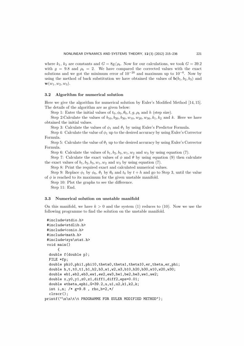
where k1, k2 are constants and G = 8g/ρb. Now for our calculations, we took G = 39.2with g = 9.8 and ρb = 2. We have compared the corrected values with the exactsolutions and we got the minimum error of 10−20 and maximum up to 10−6. Now byusing the method of back substitution we have obtained the values of b(b1, b2, b3) andw(w1, w2, w3).
3.2 Algorithm for numerical solution
Here we give the algorithm for numerical solution by Euler’s Modified Method [14, 15].The details of the algorithm are as given below:
Step 1: Enter the initial values of t0, φ0, θ0, t, g, ρb and h (step size).Step 2:Calculate the values of b10, b20, b30, w10, w20, w30, k1, k2 and k. Here we have
obtained the initial values.Step 3: Calculate the values of φ1 and θ1 by using Euler’s Predictor Formula.Step 4: Calculate the value of φ1 up to the desired accuracy by using Euler’s Corrector
Formula.Step 5: Calculate the value of θ1 up to the desired accuracy by using Euler’s Corrector
Formula.Step 6: Calculate the values of b1, b2, b3, w1, w2 and w3 by using equation (7).Step 7: Calculate the exact values of φ and θ by using equation (9) then calculate
the exact values of b1, b2, b3, w1, w2 and w3 by using equation (7).Step 8: Print the required exact and calculated numerical values.Step 9: Replace φ1 by φ0, θ1 by θ0 and t0 by t+ h and go to Step 3, until the value
of φ is reached to its maximum for the given unstable manifold.Step 10: Plot the graphs to see the difference.Step 11: End.
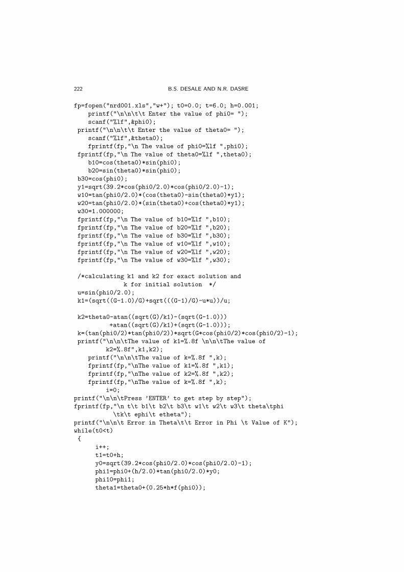
3.3 Numerical solution on unstable manifold
On this manifold, we have k > 0 and the system (1) reduces to (10). Now we use thefollowing programme to find the solution on the unstable manifold.
#include<stdio.h>
#include<stdlib.h>
#include<conio.h>
#include<math.h>
#include<sys\stat.h>
void main()
double f(double p);
FILE *fp;
double phi0,phi1,phi10,theta0,theta1,theta10,er_theta,er_phi;
double h,t,t0,t1,b1,b2,b3,w1,w2,w3,b10,b20,b30,w10,w20,w30;
double eb1,eb2,eb3,ew1,ew2,ew3,be1,be2,be3,we1,we2;
double x,y0,y1,z0,z1,diff1,diff2,eps=0.01;
double etheta,ephi,G=39.2,u,u1,u2,k1,k2,k;
int i,n; /* g=9.8 , rho_b=2,*/
clrscr();
printf("\n\n\t\t PROGRAMME FOR EULER MODIFIED METHOD");
222 B.S. DESALE AND N.R. DASRE
fp=fopen("nrd001.xls","w+"); t0=0.0; t=6.0; h=0.001;
printf("\n\n\t\t Enter the value of phi0= ");
scanf("%lf",&phi0);
printf("\n\n\t\t Enter the value of theta0= ");
scanf("%lf",&theta0);
fprintf(fp,"\n The value of phi0=%lf ",phi0);
fprintf(fp,"\n The value of theta0=%lf ",theta0);
b10=cos(theta0)*sin(phi0);
b20=sin(theta0)*sin(phi0);
b30=cos(phi0);
y1=sqrt(39.2*cos(phi0/2.0)*cos(phi0/2.0)-1);
w10=tan(phi0/2.0)*(cos(theta0)-sin(theta0)*y1);
w20=tan(phi0/2.0)*(sin(theta0)+cos(theta0)*y1);
w30=1.000000;
fprintf(fp,"\n The value of b10=%lf ",b10);
fprintf(fp,"\n The value of b20=%lf ",b20);
fprintf(fp,"\n The value of b30=%lf ",b30);
fprintf(fp,"\n The value of w10=%lf ",w10);
fprintf(fp,"\n The value of w20=%lf ",w20);
fprintf(fp,"\n The value of w30=%lf ",w30);
/*calculating k1 and k2 for exact solution and
k for initial solution */
u=sin(phi0/2.0);
k1=(sqrt((G-1.0)/G)+sqrt(((G-1)/G)-u*u))/u;
k2=theta0-atan((sqrt(G)/k1)-(sqrt(G-1.0)))
+atan((sqrt(G)/k1)+(sqrt(G-1.0)));
k=(tan(phi0/2)*tan(phi0/2))*sqrt(G*cos(phi0/2)*cos(phi0/2)-1);
printf("\n\n\tThe value of k1=%.8f \n\n\tThe value of
k2=%.8f",k1,k2);
printf("\n\n\tThe value of k=%.8f ",k);
fprintf(fp,"\nThe value of k1=%.8f ",k1);
fprintf(fp,"\nThe value of k2=%.8f ",k2);
fprintf(fp,"\nThe value of k=%.8f ",k);
i=0;
printf("\n\n\tPress ’ENTER’ to get step by step");
fprintf(fp,"\n t\t b1\t b2\t b3\t w1\t w2\t w3\t theta\tphi
\tk\t ephi\t etheta");
printf("\n\n\t Error in Theta\t\t Error in Phi \t Value of K");
while(t0<t)
i++;
t1=t0+h;
y0=sqrt(39.2*cos(phi0/2.0)*cos(phi0/2.0)-1);
phi1=phi0+(h/2.0)*tan(phi0/2.0)*y0;
phi10=phi1;
theta1=theta0+(0.25*h*f(phi0));
NONLINEAR DYNAMICS AND SYSTEMS THEORY, 12 (3) (2012) 215–236 223
theta10=theta1;
/* Calculation of phi by modified formula */
do
y0=sqrt(39.2*cos(phi0/2.0)*cos(phi0/2.0)-1);
y1=sqrt(39.2*cos(phi10/2.0)*cos(phi10/2.0)-1);
phi1=phi0+(0.25*h)*((tan(phi0/2.0)*y0)+(tan(phi10/2.0)*y1));
diff1=fabs(phi1-phi10);
phi10=phi1;
while(diff1>eps);
k=(tan(phi1/2)*tan(phi1/2)) *sqrt(G*cos(phi1/2)*cos(phi1/2)-1);
/* Calculation of theta by modified formula */
do
theta1=theta0+(0.125*h)*(f(phi0)+f(phi1));
diff2=fabs(theta10-theta1);
while(diff2>eps);
/* Calculation of an approximate solution what we need */
b1=cos(theta1)*sin(phi1);
b2=sin(theta1)*sin(phi1);
b3=cos(phi1);
y1=sqrt(39.2*cos(phi1/2.0)*cos(phi1/2.0)-1);
w1=tan(phi1/2.0)*(cos(theta1)-sin(theta1)*y1);
w2=tan(phi1/2.0)*(sin(theta1)+cos(theta1)*y1);
w3=1.000000;
/* calculation of exact solution */
ephi=2*asin((2*k1*sqrt((G-1)/G)*exp(-(t1/4)*sqrt(G-1)))
/(1+k1*k1*exp(-(t1/2)*sqrt(G-1))));
u1=atan((sqrt(G)*exp((t1/4)*sqrt(G-1)))/k1-sqrt(G-1));
u2=atan((sqrt(G)*exp((t1/4)*sqrt(G-1)))/k1+sqrt(G-1));
etheta=(t1/4)+u1-u2+k2;
k=(tan(etheta/2)*tan(etheta/2))
*sqrt(G*cos(etheta/2)*cos(etheta/2)-1);
/* calculation of error in theta and phi*/
er_theta=fabs(theta1-etheta);
er_phi=fabs(phi1-ephi);
/* calculation of B and W */
be1=cos(etheta)*sin(ephi);
be2=sin(etheta)*sin(ephi);
be3=cos(ephi);
y1=sqrt(39.2*cos(ephi/2.0)*cos(ephi/2.0)-1);
we1=tan(ephi/2.0)*(cos(etheta)-sin(etheta)*y1);
we2=tan(ephi/2.0)*(sin(etheta)+cos(etheta)*y1);
224 B.S. DESALE AND N.R. DASRE
fprintf(fp,"\n%lf\t%lf\t%lf\t%lf\t%lf\t%lf\t%lf\t%lf\t%lf
\t%lf\t%lf\t%lf", t1, b1, b2, b3, w1, w2, w3,
theta1, phi1, k, etheta, ephi);
printf("\n\n\t%.20lf\t%.20lf\t%lf",er_theta,er_phi,k);
phi0=phi1;
theta0=theta1;
t0=t1;
getch();
double f(double p)
double p_dash;
p_dash=(1.0/cos(p/2.0))*(1.0/cos(p/2.0));
return(p_dash);
3.4 Numerical solution on stable manifold
On this manifold, we have k < 0 and the system (1) reduces to (12). Now we use thefollowing programme to find the solution on the stable manifold.
#include<stdio.h>
#include<stdlib.h>
#include<conio.h>
#include<math.h>
#include<sys\stat.h>
void main()
double f(double p);
FILE *fp;
double phi0,phi1,phi10,theta0,theta1,theta10,er_theta,er_phi;
double h,t,t0,t1,b1,b2,b3,w1,w2,w3,b10,b20,b30,w10,w20,w30;
double eb1,eb2,eb3,ew1,ew2,ew3,be1,be2,be3,we1,we2;
double x,y0,y1,z0,z1,diff1,diff2,eps=0.01;
double etheta,ephi,G=39.2,u,u1,u2,k1,k2,k;
int i,n; /* g=9.8 , rho_b=2,*/
clrscr(); printf("\n\n\t\t PROGRAMME FOR EULER MODIFIED METHOD");
fp=fopen("nrd001.xls","w+"); t0=0.0; t=6.0; h=0.001;
printf("\n\n\t\t Enter the value of phi0= ");
scanf("%lf",&phi0);
printf("\n\n\t\t Enter the value of theta0= ");
scanf("%lf",&theta0);
fprintf(fp,"\n The value of phi0=%lf ",phi0);
fprintf(fp,"\n The value of theta0=%lf ",theta0);
b10=cos(theta0)*sin(phi0);
b20=sin(theta0)*sin(phi0);
b30=cos(phi0);
y1=sqrt(39.2*cos(phi0/2.0)*cos(phi0/2.0)-1);
w10=tan(phi0/2.0)*(cos(theta0)+sin(theta0)*y1);
w20=tan(phi0/2.0)*(sin(theta0)-cos(theta0)*y1);
NONLINEAR DYNAMICS AND SYSTEMS THEORY, 12 (3) (2012) 215–236 225
w30=1.000000;
fprintf(fp,"\n The value of b10=%lf ",b10);
fprintf(fp,"\n The value of b20=%lf ",b20);
fprintf(fp,"\n The value of b30=%lf ",b30);
fprintf(fp,"\n The value of w10=%lf ",w10);
fprintf(fp,"\n The value of w20=%lf ",w20);
fprintf(fp,"\n The value of w30=%lf ",w30);
/*calculating k1 and k2 for exact solution
and k for initial solution */
u=sin(phi0/2.0);
k1=(sqrt((G-1.0)/G)+sqrt(((G-1)/G)-u*u))/u;
k2=theta0-atan((sqrt(G)/k1)-(sqrt(G-1.0)))
+atan((sqrt(G)/k1)+(sqrt(G-1.0)));
k= - (tan(phi0/2)*tan(phi0/2))
*sqrt(G*cos(phi0/2)*cos(phi0/2)-1);
printf("\n\n\tThe value of k1=%.8f \n\n\tThe value of
k2=%.8f",k1,k2);
printf("\n\n\tThe value of k=%.8f ",k);
fprintf(fp,"\nThe value of k1=%.8f ",k1);
fprintf(fp,"\nThe value of k2=%.8f ",k2);
fprintf(fp,"\nThe value of k=%.8f ",k);
i=0;
printf("\n\n\tPress ’ENTER’ to get step by step");
fprintf(fp,"\n t\t b1\t b2\t b3\t w1\t w2\t w3\t theta\t phi
\tk\t ephi\t etheta");
printf("\n\n\t Error in Theta\t\t Error in Phi \t Value of K");
while(t0<t)
i++;
t1=t0+h;
y0=sqrt(39.2*cos(phi0/2.0)*cos(phi0/2.0)-1);
phi1=phi0-(h/2.0)*tan(phi0/2.0)*y0;
phi10=phi1;
theta1=theta0+(0.25*h*f(phi0));
theta10=theta1;
/* Calculation of phi by modified formula */
do
y0=sqrt(39.2*cos(phi0/2.0)*cos(phi0/2.0)-1);
y1=sqrt(39.2*cos(phi10/2.0)*cos(phi10/2.0)-1);
phi1=phi0-(0.25*h)*((tan(phi0/2.0)*y0)+(tan(phi10/2.0)*y1));
diff1=fabs(phi1-phi10);
phi10=phi1;
while(diff1>eps);
k= - (tan(phi1/2)*tan(phi1/2))
*sqrt(G*cos(phi1/2)*cos(phi1/2)-1);

226 B.S. DESALE AND N.R. DASRE
/* Calculation of theta by modified formula */
do
theta1=theta0+(0.125*h)*(f(phi0)+f(phi1));
diff2=fabs(theta10-theta1);
while(diff2>eps);
/* Calculation of an approximate solution what we need */
b1=cos(theta1)*sin(phi1);
b2=sin(theta1)*sin(phi1);
b3=cos(phi1);
y1=sqrt(39.2*cos(phi1/2.0)*cos(phi1/2.0)-1);
w1=tan(phi1/2.0)*(cos(theta1)+sin(theta1)*y1);
w2=tan(phi1/2.0)*(sin(theta1)-cos(theta1)*y1);
w3=1.000000;
/* calculation of exact solution */
ephi=2*asin((2*k1*sqrt((G-1)/G)*exp(-(t1/4)*sqrt(G-1)))
/(1+k1*k1*exp(-(t1/2)*sqrt(G-1))));
u1=atan((sqrt(G)*exp((t1/4)*sqrt(G-1)))/k1-sqrt(G-1));
u2=atan((sqrt(G)*exp((t1/4)*sqrt(G-1)))/k1+sqrt(G-1));
etheta=(t1/4)+u1-u2+k2;
k=-(tan(etheta/2)*tan(etheta/2))
*sqrt(G*cos(etheta/2)*cos(etheta/2)-1);
/* calculation of error in theta and phi*/
er_theta=fabs(theta1-etheta);
er_phi=fabs(phi1-ephi);
/* calculation of B and W */
be1=cos(etheta)*sin(ephi);
be2=sin(etheta)*sin(ephi);
be3=cos(ephi);
y1=sqrt(39.2*cos(ephi/2.0)*cos(ephi/2.0)-1);
we1=tan(ephi/2.0)*(cos(etheta)+sin(etheta)*y1);
we2=tan(ephi/2.0)*(sin(etheta)-cos(etheta)*y1);
fprintf(fp,"\n%lf\t%lf\t%lf\t%lf\t%lf\t%lf\t%lf
\t%lf\t%lf\t%lf\t%lf\t%lf",t1,b1,b2,b3,w1,w2,
w3, theta1, k, etheta, ephi);
printf("\n\n\t%.20lf\t%.20lf\t%lf",er_theta,er_phi,k);
phi0=phi1;
theta0=theta1;
t0=t1;
getch();
double f(double p)
double p_dash;
p_dash=(1.0/cos(p/2.0))*(1.0/cos(p/2.0));
return(p_dash);
NONLINEAR DYNAMICS AND SYSTEMS THEORY, 12 (3) (2012) 215–236 227
4 Experimental Results
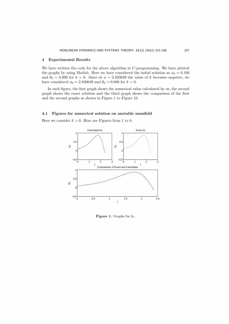
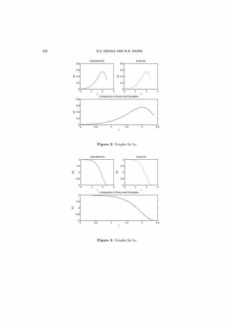
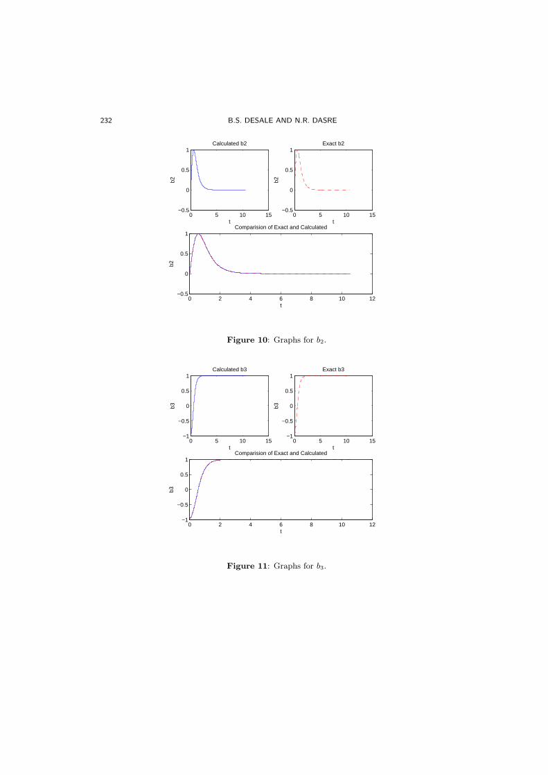
We have written the code for the above algorithm in C-programming. We have plottedthe graphs by using Matlab. Here we have considered the initial solution as φ0 = 0.100and θ0 = 0.000 for k > 0. Since at φ = 2.820649 the value of k becomes negative, wehave considered φ0 = 2.820649 and θ0 = 0.000 for k > 0.
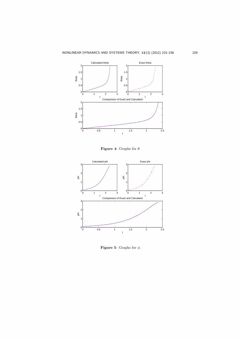
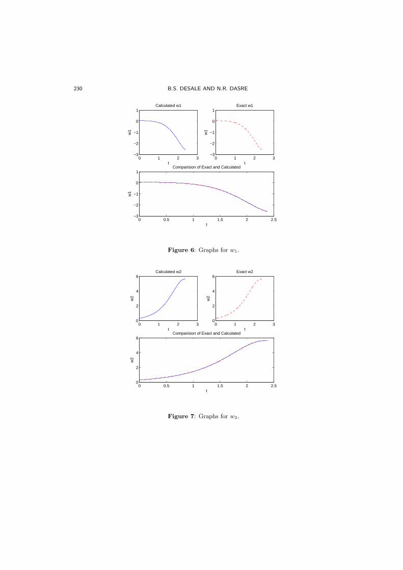
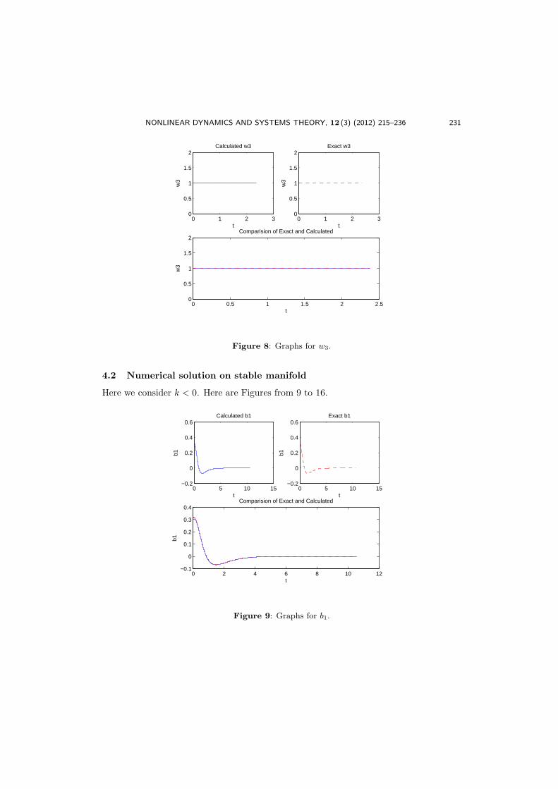
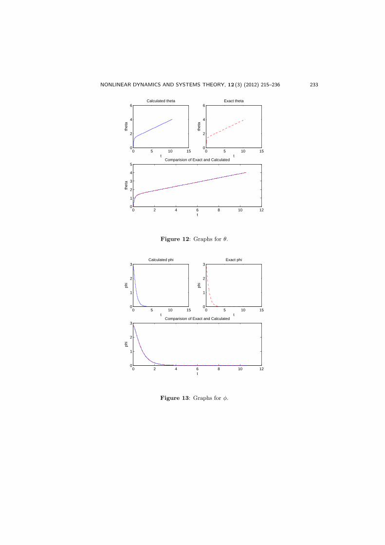
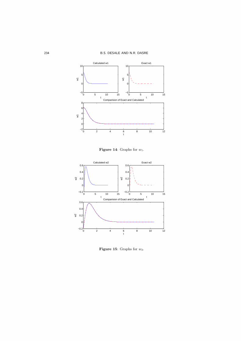
In each figure, the first graph shows the numerical value calculated by us, the secondgraph shows the exact solution and the third graph shows the comparison of the firstand the second graphs as shown in Figure 1 to Figure 16.
4.1 Figures for numerical solution on unstable manifold
Here we consider k > 0. Here are Figures from 1 to 8.
0 1 2 3−0.5
0
0.5
1
t
b1
Calculated b1
0 1 2 3−0.5
0
0.5
1
t
b1
Exact b1
0 0.5 1 1.5 2 2.5−0.5
0
0.5
1
t
b1
Comparision of Exact and Calculated
Figure 1: Graphs for b1.
228 B.S. DESALE AND N.R. DASRE
0 1 2 30
0.2
0.4
0.6
0.8
t
b2
Calculated b2
0 1 2 30
0.2
0.4
0.6
0.8
t
b2
Exact b2
0 0.5 1 1.5 2 2.50
0.2
0.4
0.6
0.8
t
b2
Comparision of Exact and Calculated
Figure 2: Graphs for b2.
0 1 2 3−1
−0.5
0
0.5
1
t
b3
Calculated b3
0 1 2 3−1
−0.5
0
0.5
1
t
b3
Exact b3
0 0.5 1 1.5 2 2.5−1
−0.5
0
0.5
1
t
b3
Comparision of Exact and Calculated
Figure 3: Graphs for b3.
NONLINEAR DYNAMICS AND SYSTEMS THEORY, 12 (3) (2012) 215–236 229
0 1 2 30
0.5
1
1.5
2
t
thet
a
Calculated theta
0 1 2 30
0.5
1
1.5
2
t
thet
a
Exact theta
0 0.5 1 1.5 2 2.50
0.5
1
1.5
2
t
thet
a
Comparision of Exact and Calculated
Figure 4: Graphs for θ.
0 1 2 30
1
2
3
t
phi
Calculated phi
0 1 2 30
1
2
3
t
phi
Exact phi
0 0.5 1 1.5 2 2.50
1
2
3
t
phi
Comparision of Exact and Calculated
Figure 5: Graphs for φ.
230 B.S. DESALE AND N.R. DASRE
0 1 2 3−3
−2
−1
0
1
t
w1
Calculated w1
0 1 2 3−3
−2
−1
0
1
t
w1
Exact w1
0 0.5 1 1.5 2 2.5−3
−2
−1
0
1
t
w1
Comparision of Exact and Calculated
Figure 6: Graphs for w1.
0 1 2 30
2
4
6
t
w2
Calculated w2
0 1 2 30
2
4
6
t
w2
Exact w2
0 0.5 1 1.5 2 2.50
2
4
6
t
w2
Comparision of Exact and Calculated
Figure 7: Graphs for w2.
NONLINEAR DYNAMICS AND SYSTEMS THEORY, 12 (3) (2012) 215–236 231
0 1 2 30
0.5
1
1.5
2
t
w3
Calculated w3
0 1 2 30
0.5
1
1.5
2
t
w3
Exact w3
0 0.5 1 1.5 2 2.50
0.5
1
1.5
2
t
w3
Comparision of Exact and Calculated
Figure 8: Graphs for w3.
4.2 Numerical solution on stable manifold
Here we consider k < 0. Here are Figures from 9 to 16.
0 5 10 15−0.2
0
0.2
0.4
0.6
t
b1
Calculated b1
0 5 10 15−0.2
0
0.2
0.4
0.6
t
b1
Exact b1
0 2 4 6 8 10 12−0.1
0
0.1
0.2
0.3
0.4
t
b1
Comparision of Exact and Calculated
Figure 9: Graphs for b1.
232 B.S. DESALE AND N.R. DASRE
0 5 10 15−0.5
0
0.5
1
t
b2
Calculated b2
0 5 10 15−0.5
0
0.5
1
t
b2
Exact b2
0 2 4 6 8 10 12−0.5
0
0.5
1
t
b2
Comparision of Exact and Calculated
Figure 10: Graphs for b2.
0 5 10 15−1
−0.5
0
0.5
1
t
b3
Calculated b3
0 5 10 15−1
−0.5
0
0.5
1
t
b3
Exact b3
0 2 4 6 8 10 12−1
−0.5
0
0.5
1
t
b3
Comparision of Exact and Calculated
Figure 11: Graphs for b3.
NONLINEAR DYNAMICS AND SYSTEMS THEORY, 12 (3) (2012) 215–236 233
0 5 10 150
2
4
6
t
thet
a
Calculated theta
0 5 10 150
2
4
6
t
thet
a
Exact theta
0 2 4 6 8 10 120
1
2
3
4
5
t
thet
a
Comparision of Exact and Calculated
Figure 12: Graphs for θ.
0 5 10 150
1
2
3
t
phi
Calculated phi
0 5 10 150
1
2
3
t
phi
Exact phi
0 2 4 6 8 10 120
1
2
3
t
phi
Comparision of Exact and Calculated
Figure 13: Graphs for φ.
234 B.S. DESALE AND N.R. DASRE
0 5 10 15−5
0
5
10
t
w1
Calculated w1
0 5 10 15−5
0
5
10
t
w1
Exact w1
0 2 4 6 8 10 12−2
0
2
4
6
8
t
w1
Comparision of Exact and Calculated
Figure 14: Graphs for w1.
0 5 10 15−0.2
0
0.2
0.4
0.6
t
w2
Calculated w2
0 5 10 15−0.2
0
0.2
0.4
0.6
t
w2
Exact w2
0 2 4 6 8 10 12−0.2
0
0.2
0.4
0.6
t
w2
Comparision of Exact and Calculated
Figure 15: Graphs for w2.
NONLINEAR DYNAMICS AND SYSTEMS THEORY, 12 (3) (2012) 215–236 235
0 5 10 150
0.5
1
1.5
2
t
w3
Calculated w1
0 5 10 150
0.5
1
1.5
2
t
w3
Exact w3
0 2 4 6 8 10 120
0.5
1
1.5
2
t
w3
Comparision of Exact and Calculated
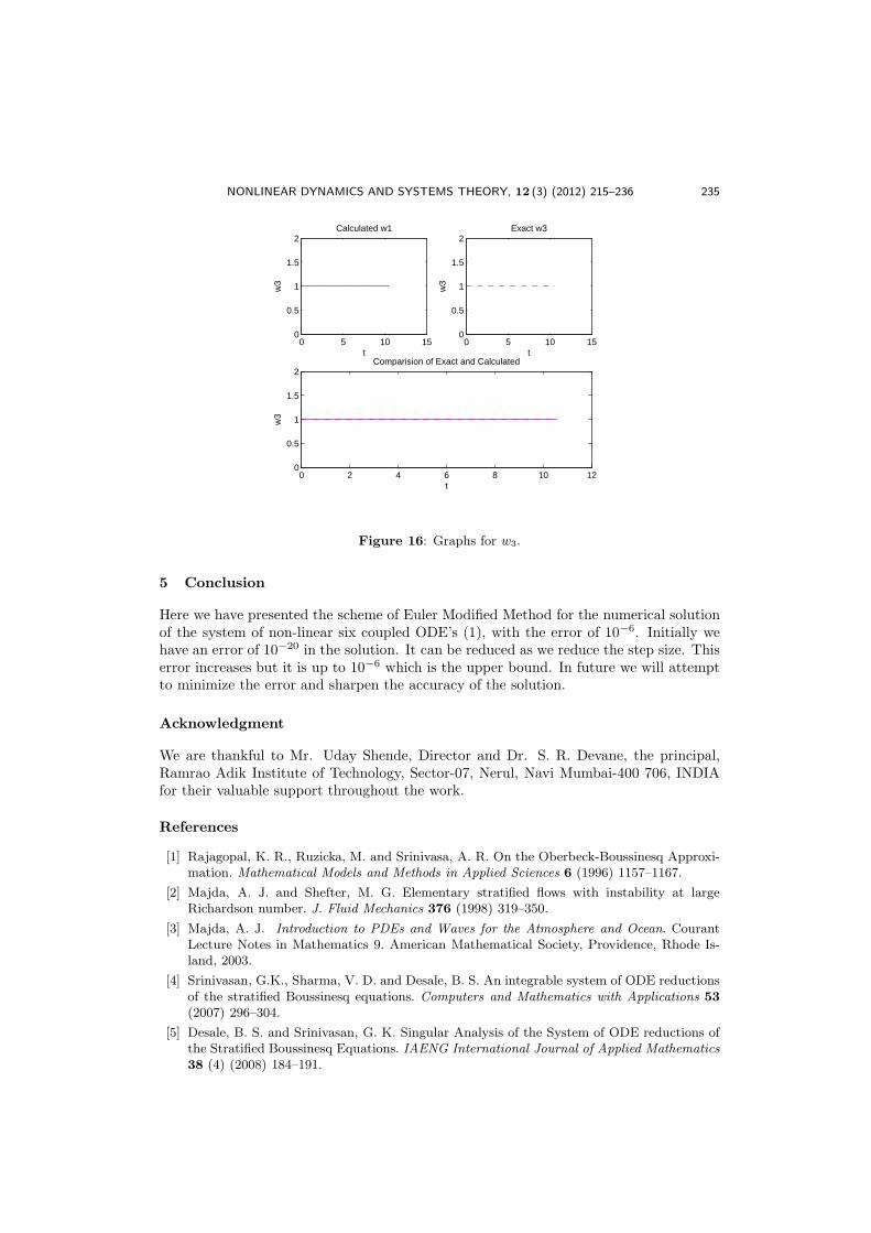
Figure 16: Graphs for w3.
5 Conclusion
Here we have presented the scheme of Euler Modified Method for the numerical solutionof the system of non-linear six coupled ODE’s (1), with the error of 10−6. Initially wehave an error of 10−20 in the solution. It can be reduced as we reduce the step size. Thiserror increases but it is up to 10−6 which is the upper bound. In future we will attemptto minimize the error and sharpen the accuracy of the solution.
Acknowledgment
We are thankful to Mr. Uday Shende, Director and Dr. S. R. Devane, the principal,Ramrao Adik Institute of Technology, Sector-07, Nerul, Navi Mumbai-400 706, INDIAfor their valuable support throughout the work.
References
[1] Rajagopal, K. R., Ruzicka, M. and Srinivasa, A. R. On the Oberbeck-Boussinesq Approxi-mation. Mathematical Models and Methods in Applied Sciences 6 (1996) 1157–1167.
[2] Majda, A. J. and Shefter, M. G. Elementary stratified flows with instability at largeRichardson number. J. Fluid Mechanics 376 (1998) 319–350.
[3] Majda, A. J. Introduction to PDEs and Waves for the Atmosphere and Ocean. CourantLecture Notes in Mathematics 9. American Mathematical Society, Providence, Rhode Is-land, 2003.
[4] Srinivasan, G.K., Sharma, V. D. and Desale, B. S. An integrable system of ODE reductionsof the stratified Boussinesq equations. Computers and Mathematics with Applications 53(2007) 296–304.
[5] Desale, B. S. and Srinivasan, G. K. Singular Analysis of the System of ODE reductions ofthe Stratified Boussinesq Equations. IAENG International Journal of Applied Mathematics
38 (4) (2008) 184–191.
236 B.S. DESALE AND N.R. DASRE
[6] Desale, B. S. Complete Analysis of an Ideal Rotating Uniformly Stratified System of ODEs.Nonlinear Dyanamics and Systems Theory 9(3) (2009) 263–275.
[7] Desale, B. S. and Sharma, V. Special Solutions to Rotating Stratified Boussinesq Equations.Nonlinear Dyanamics and Systems Theory 10(1) (2010) 29–38.
[8] Desale, B. S. and Patil, K. D. Painleve’ Test to a Reduced System of Six Coupled NonlinearODEs. Nonlinear Dyanamics and Systems Theory 10(4) (2010) 349–361.
[9] Burton, T. A. and Zhang, B. Periodic solutions of Singular Integral Equations. Nonlinear
Dyanamics and Systems Theory 11(1) (2011) 113–123.
[10] Biswas, M. H. A., Rahman, M. A. and Das, T. Optical Soliton in Nonlinear Dynamics andIt’s Graphical Representation. Nonlinear Dyanamics and Systems Theory 11(4) (2011)383–396.
[11] Desale, B. S. An integrable system of reduced ODEs of Stratified Boussinesq Equations.Ph. D. thesis, Indian Institute of Technology Bombay. Powai, Mumbai, 2007.
[12] Mathews, J. H. Numerical Methods for Mathematics, Science and Engineering, 2nd Edition.Prentice Hall of India, New Delhi, 1994.
[13] Kreyszig, E. Advanced Engineering Mathematics, 9th Edition. Wiley India (P) Ltd., NewDelhi, 2010.
[14] Jain, M. K. and Iyengar, S. R. K. Numerical Methods for scientific and engineering com-
putation, 3rd Edition. New Age International (P) Ltd., Mumbai, 2001.
[15] Sastry, S. S. Introductory Methods of Numerical Analysis. Prentice Hall of India (P) Ltd.,New Delhi, 2001.
Nonlinear Dynamics and Systems Theory, 12 (3) (2012) 237–250
Euler Solutions for Integro Differential Equations with
Retardation and Anticipation
J. Vasundhara Devi ∗ and Ch.V. Sreedhar
GVP–Prof. V. Lakshmikantham Institute for Advanced Studies,
Department of Mathematics, GVP College of Engineering, Visakhapatnam, AP, India.
Received: July 19, 2011; Revised: July 11, 2012
Abstract: In this paper, we obtain results for Euler solution for integro differentialequation with retardation and anticipation.
Keywords: integro differential equations with retardation and anticipation; Euler
solutions.
Mathematics Subject Classification (2010): 45J99, 47G20.
1 Introduction
Integro differential equations arise quite frequently as mathematical models in diversedisciplines. The study of integro differential equations has been attracting the attentionof many scientific researchers due to its potential as a better model to represent phys-ical phenomena in various disciplines. Much work has been done in the existence anduniqueness of solutions for integro differential equations see [2, 3, 6, 7, 8, 12]. All theseresults are abstract in the sense that there is no specific procedure to obtain a solutionof the considered equations, so the Euler solutions for integro differential equations arestudied [4].
In many physical phenomena the both past history and future play an importantrole along with the present state and hence an appropriate model of the phenomena willbe one that involves past history and future expectation also. This led to the study ofsystems involving both retardation and anticipation, for example, see [1]. The existence ofEuler solutions have been studied for set differential equations [11], for causal differentialequations [10], for delay differential equations [5], due to the inherited simplicity in itsidea which paves a path for obtaining a solution of the given system. In this paper,
∗ Corresponding author: mailto:[email protected]
c© 2012 InforMath Publishing Group/1562-8353 (print)/1813-7385 (online)/http://e-ndst.kiev.ua237
238 J. VASUNDHARA DEVI AND CH.V. SREEDHAR
we give an approach to obtaining the solution of the integro differential equation withretardation and anticipation under continuity conditions.
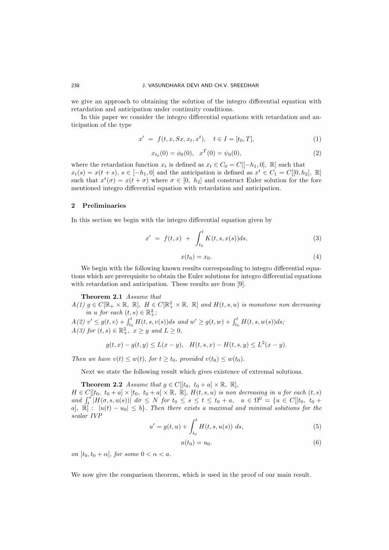
In this paper we consider the integro differential equations with retardation and an-ticipation of the type
x′ = f(t, x, Sx, xt, xt), t ∈ I = [t0, T ], (1)
xt0(0) = φ0(0), xT (0) = ψ0(0), (2)
where the retardation function xt is defined as xt ∈ C0 = C[[−h1, 0], R] such thatxt(s) = x(t + s), s ∈ [−h1, 0] and the anticipation is defined as xt ∈ C1 = C[[0, h2], R]such that xt(σ) = x(t + σ) where σ ∈ [0, h2] and construct Euler solution for the forementioned integro differential equation with retardation and anticipation.
2 Preliminaries
In this section we begin with the integro differential equation given by
x′ = f(t, x) +
∫ t
t0
K(t, s, x(s))ds, (3)
x(t0) = x0. (4)
We begin with the following known results corresponding to integro differential equa-tions which are prerequisite to obtain the Euler solutions for integro differential equationswith retardation and anticipation. These results are from [9].
Theorem 2.1 Assume thatA(1) g ∈ C[R+ × R, R], H ∈ C[R2
+ × R, R] and H(t, s, u) is monotone non decreasingin u for each (t, s) ∈ R
2+;
A(2) v′ ≤ g(t, v) +∫ t
t0H(t, s, v(s))ds and w′ ≥ g(t, w) +
∫ t
t0H(t, s, w(s))ds;
A(3) for (t, s) ∈ R2+, x ≥ y and L ≥ 0,
g(t, x)− g(t, y) ≤ L(x− y), H(t, s, x)−H(t, s, y) ≤ L2(x− y).
Then we have v(t) ≤ w(t), for t ≥ t0, provided v(t0) ≤ w(t0).
Next we state the following result which gives existence of extremal solutions.
Theorem 2.2 Assume that g ∈ C[[t0, t0 + a]× R, R],H ∈ C[[t0, t0 + a]× [t0, t0 + a]× R, R], H(t, s, u) is non decreasing in u for each (t, s)and
∫ s
t|H(σ, s, u(s))| dσ ≤ N for t0 ≤ s ≤ t ≤ t0 + a, u ∈ Ω0 = u ∈ C[[t0, t0 +
a], R] : |u(t) − u0| ≤ b. Then there exists a maximal and minimal solutions for thescalar IVP
u′ = g(t, u) +
∫ t
t0
H(t, s, u(s)) ds, (5)
u(t0) = u0. (6)
on [t0, t0 + α], for some 0 < α < a.
We now give the comparison theorem, which is used in the proof of our main result.
NONLINEAR DYNAMICS AND SYSTEMS THEORY, 12 (3) (2012) 237–250 239
Theorem 2.3 Assume that g ∈ C[R2+, R], H ∈ C[R3
+, R], H(t, s, u) is non de-
creasing in u for each (t, s) and for t ≥ t0, D−m(t) ≤ g(t,m(t)) +∫ t
t0H(t, s,m(s))ds,
where m ∈ C[R+, R] and D−m(t) = limh→0−inf [m(t+h)−m(t)
h]. Suppose that γ(t) is
the maximal solution of u′ = g(t, u(t)) +∫ t
t0H(t, s, u(s))ds, u(t0) = u0 ≥ 0, existing on
[t0,∞). Then m(t) ≤ γ(t), for t ≥ t0, provided m(t0) ≤ u0.
Before we proceed further, we state the following known result relating to integrodifferential equations, which is indirectly used in our work.
Theorem 2.4 Let E1 be an open (t, u)-set in Rn+1 and let f ∈ C[E1,R
n],K ∈ C[E1 ×R
n+,R
n+] and x(t) be a solution of (3) and (4)on some interval t0 ≤ t ≤ a0.
Then x(t) can be extended as a solution to the boundary of E1.
We now present a theorem relating to the largest interval of existence of maximalsolutions in a particular setup.
Theorem 2.5 Let the hypothesis of Theorem 2.2 hold. Suppose that the largestinterval of existence of the maximal solution r(t) of (5) and (6) is [t0, t0 + a). Thenthere is an ǫ0 > 0 such that 0 < ǫ < ǫ0, the maximal solution r(t, ǫ) of
u′ = g(t, u) +
∫ t
t0
H(t, s, u(s)) ds+ ǫ, (7)
u(t0) = u0 + ǫ ≥ 0, (8)
exists over [t0, t1] ⊂ [t0, t0 + a) and limǫ→0 r(t, ǫ) = r(t) uniformly on [t0, t1].
3 Comparison Theorems
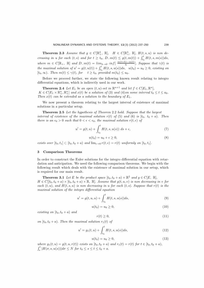
In order to construct the Euler solutions for the integro differential equation with retar-dation and anticipation. We need the following comparison theorems. We begin with thefollowing result which deals with the existence of maximal solution in our setup, whichis required for our main result.
Theorem 3.1 Let E be the product space [t0, t0 + a)× R2 and g ∈ C[E, R],
H ∈ C[[t0, t0 + a)× [t0, t0 + a)×R, R]. Assume that g(t, u, v) is non decreasing in v foreach (t, u), and H(t, s, u) is non decreasing in u for each (t, s). Suppose that r(t) is themaximal solution of the integro differential equation
u′ = g(t, u, u) +
∫ t
t0
H(t, s, u(s))ds, (9)
u(t0) = u0 ≥ 0, (10)
existing on [t0, t0 + a) andr(t) ≥ 0, (11)
on [t0, t0 + a). Then the maximal solution r1(t) of
u′ = g1(t, u) +
∫ t
t0
H(t, s, u(s))ds, (12)
u(t0) = u0 ≥ 0, (13)
where g1(t, u) = g(t, u, r(t)) exists on [t0, t0 + a) and r1(t) = r(t) for t ∈ [t0, t0 + a),∫ t
s|H(σ, s, u(s))|dσ ≤ N for t0 ≤ s ≤ t ≤ t0 + a.
240 J. VASUNDHARA DEVI AND CH.V. SREEDHAR
Proof. Consider the scalar integro differential equation (12) and (13). By Theorem2.2 there exists a maximal solution r1(t) of (12) and (13) in the interval [t0, t0+α), where0 < α < a and by Theorem 2.4 this maximal solution can be extended from [t0, t0 + α)to [t0, t0 + a). This implies that either r1(t) is defined over [t0, t0 + a) or there exists at1 < t0 + a such that
|r1(tk)| → ∞, (14)
for a certain sequence tk, such that tk → t−1 as k → ∞. Observe that
r′(t) = g(t, r(t), r(t)) +
∫ t
t0
H(t, s, r(s))ds = g1(t, r(t)) +
∫ t
t0
H(t, s, r(s))ds,
and Theorem 2.3 yields thatr(t) ≤ r1(t), (15)
as far as r1(t) exists. Now using the relations (11), (14) and (15), we have
|r1(tk)| → +∞ (16)
for some sequence tk, such that tk → t−1 as k → ∞. We shall prove that (16) does nothold. Since the largest interval of existence of maximal solution r(t) of the scalar integrodifferential equaiton (9) and (10) is [t0, t0+a), so by Theorem 2.5 there is an ǫ0 > 0 suchthat 0 < ǫ < ǫ0 and the maximal solution r(t, ǫ) of
u′ = g(t, u, u) +
∫ t
t0
H(t, s, u(s)) ds+ ǫ, (17)
u(t0) = u0 + ǫ ≥ 0, (18)
exists over [t0, t1+ν] ⊂ [t0, t0+a), ν > 0, t1+ν < t0+a. From the relations (17), (18)we get
r′(t, ǫ) > g(t, r(t, ǫ), r(t, ǫ)) +
∫ t
t0
H(t, s, r(s, ǫ))ds
and r(t0) = u0 < u0 + ǫ = r(t0, ǫ). So
r(t0) < r(t0, ǫ).
Now applying Theorem 2.1 we conclude that
r(t) < r(t, ǫ), (19)
for t ∈ [t0, t1 + ν]. Since g is non decreasing in v, we arrive at r′(t, ǫ) > g1(t, r(t, ǫ)) +∫ t
t0H(t, s, r(s, ǫ))ds, for t ∈ [t0, t1 + ν]. But
r′1(t) = g1(t, r1(t)) +
∫ t
t0
H(t, s, r1(s))ds,
for t ∈ [t0, t1] and r1(t0) = u0 < u0 + ǫ = r(t0, ǫ), so
r1(t) < r(t, ǫ),
NONLINEAR DYNAMICS AND SYSTEMS THEORY, 12 (3) (2012) 237–250 241
for t ∈ [t0, t1]. Since r(t, ǫ) exists on [t0, t1 + ν], ν > 0. This leads to a contradiction to(16). Hence r1(t) exists on [t0, t0 + a). Thus r(t) ≤ r1(t) for t ∈ [t0, t0 + a). Furthermore,
r′1(t) = g1(t, r1(t)) +
∫ t
t0
H(t, s, r1(s))ds
= g(t, r1(t), r(t)) +
∫ t
t0
H(t, s, r1(s))ds.
From the monotonic character of g in v, and from the relation (15), we get
r′1(t) = g(t, r1(t), r(t)) +
∫ t
t0
H(t, s, r1(s))ds
≤ g(t, r1(t), r1(t)) +
∫ t
t0
H(t, s, r1(s))ds.
Now using Theorem 2.3, we find that
r1(t) ≤ r(t) (20)
on t ∈ [t0, t0 + a), which implies along with the relation (15) that r1(t) = r(t) fort ∈ [t0, t0 + a).
We need the following known result in suitable form.
Theorem 3.2 Let the hypothesis of Theorem 3.1 hold and m ∈ C[[t0, t0 + a), R]such that (t,m(t), ν) ∈ E, t ∈ [t0, t0 + a) and m(t0) ≤ u0. Assume that for a fixed
Dini Derivative the inequality Dm(t) ≤ g(t,m(t), ν) +∫ t
t0H(t, s,m(s))ds, is satisfied for
t ∈ [t0, t0 + a)−S, where S denotes an at most countable subset of [t0, t0 + a). Then forall ν ≤ r(t), t ∈ [t0, t0 + a), we have m(t) ≤ r(t), for t ∈ [t0, t0 + a).
Proof. Since the hypothesis of Theorem 3.1 holds, so there exists a maximal solutionr1(t) of the scalar integro differential equation (12) and (13) with g1(t, u) = g(t, u, r(t))exists on [t0, t0 + a) and r(t) = r1(t) for t ∈ [t0, t0 + a). Let ν ≤ r(t), t ∈ [t0, t0 + a).Then using the monotonicity of g in ν we get
Dm(t) ≤ g(t,m(t), ν) +
∫ t
t0
H(t, s,m(s))ds
≤ g(t,m(t), r(t)) +
∫ t
t0
H(t, s,m(s))ds
Dm(t) ≤ g1(t,m(t)) +
∫ t
t0
H(t, s,m(s))ds,
for t ∈ [t0, t0 + a)−S, which on using Theorem 2.3 gives m(t) ≤ r(t), for t ∈ [t0, t0 + a).The following theorem is needed before we proceed further.
Theorem 3.3 Assume that m ∈ C[I, R+], g ∈ C[I × R+, R+],H ∈ C[I × I × R+, R+], H is non decreasing in u for each (t, s) and for t ∈ I = [t0, T ],
D−m(t) ≤ g(t, |m|0(t)) +∫ t
t0
H(t, s, |m|(s))ds, (21)
242 J. VASUNDHARA DEVI AND CH.V. SREEDHAR
where |m|0(t) = supt0≤s≤t|m(s)|. Suppose that r(t) = r(t, t0, u0) is the maximal solutionof the scalar integro differential equation
u′ = g(t, u) +
∫ t
t0
H(t, s, u(s))ds, (22)
u(t0) = u0 ≥ 0, (23)
existing on [t0, T ). Then m(t) ≤ r(t), t ≥ t0, provided | m(t0) |0≤ u0.
Proof. Since the largest interval of existence of maximal solution is [t0, T ) for theintegro differential equation (22) so there exists an ǫ0 > 0 such that 0 < ǫ < ǫ0, themaximal solution r(t, t0, u0, ǫ) of
u′ = g(t, u) +
∫ t
t0
H(t, s, u(s))ds+ ǫ, (24)
u(t0) = u0 + ǫ ≥ 0, (25)
existing on [t0, t1] ⊂ [t0, T ), for t1 < T and limǫ→0r(t, t0, u0, ǫ) = r(t, t0, u0) uniformlyon [t0, t1]. To prove the conclusion of the theorem, it is sufficient to show that
m(t) < r(t, t0, u0, ǫ), (26)
for t0 ≤ t ∈ I. Suppose that the relation (26) does not hold then there exists tα > t0such that m(tα) = r(tα, t0, u0, ǫ) and m(t) < r(t, t0, u0, ǫ) for t0 ≤ t < tα. this yields oncomputation,
D−m(tα) > g(tα, r(tα, t0, u0, ǫ)) +
∫ t
t0
H(tα, s, r(tα, t0, u0, ǫ))ds (27)
which is contradiction. Observe that we have used the fact that g(t, u) ≥ 0, H(t, s, u) ≥ 0implies that r(tα, t0, u0, ǫ) is non decreasing in t and
|m|0(tα) = supt0≤s≤tα |m(s)| = r(tα, t0, u0, ǫ) = m(tα),
which yields
D−m(tα) ≤ g(tα, |m|0(tα)) +∫ tα
t0
H(tα, s, |m|0(s))ds,
= g(tα, r(tα, t0, u0, ǫ)) +
∫ t
t0
H(tα, s, r(tα, t0, u0, ǫ))ds
which is contradiction to (27), and the proof is complete.
4 Euler Solutions
In this section we define an Euler solution and prove a result for its existence of integrodifferential equation with retardation and anticipation. Further we give a result whichgives conditions under which the Euler solution becomes a solution of the IVP of theintegro differential equation with retardation and anticipation.
NONLINEAR DYNAMICS AND SYSTEMS THEORY, 12 (3) (2012) 237–250 243
Consider the integro differential equation with retardation and anticipation:
x′ = f(t, x, Sx, xt, xt), (28)
xt0(0) = φ0(0), xT (0) = ψ0(0), (29)
where t ∈ I = [t0, T ], φ0 ∈ C0, ψ0 ∈ C1, f ∈ C[I × R× R× C0 × C1, R],
Sx(t) =t∫
t0
K(t, s, x)ds, K(t, s, x) ∈ C[I2 × R, R+] and C0 = C[[−h1, 0], R],
C1 = C[[0, h2], R].In order to construct the Euler Solution we consider a partition π of the interval I
and on each subinterval of the partition, we obtain a differential equation where the righthand side is a constant. This will help us to define Euler solution as a limit of a sequenceof polygonal arcs.
In order to do so we have to find a reasonable estimate of xt in the right hand sideof the differential equation (28). For this we take the anticipation as
z(t) =
xt(0), wherever | ξt(0)− φ0(0) |< M,
xt(0) +ξ(t)
j,
(30)
where j is the number of points in the partition π and
ξ(t) =
φ0(0), t ∈ [t0 − h1, t0],
φ0(0) +(ψ0(0)− φ0(0))
(T − t0)(t− t0), t ∈ [t0, T ],
ψ0(0), t ∈ [T, T + h2].
(31)
With this approximation the integro differential equation with retardation and anticipa-tion reduces to the integro differential equation with retardation only, i.e.,
x′ = f(t, x, Sx, xt, z(t)), (32)
xt0(0) = φ0(0), z(T ) = ψ0(0), (33)
for t ∈ I = [t0, T ]. Let partition of the interval [t0, T ] be given by
π = t0, t1, t2, ..., tN = T . (34)
Consider the sub interval [t0, t1] and the differential equation (32), in that subinterval.In the right hand side of (32) replace t by t0, x by x0, xt by φ0(0), z(t) by z(t0) andSx by (Sx(t0), t0) ie., in the integral replace t with t0, s with t0, x with x0, so (32)reduces to
x′ = f(t0, x0, (Sx(t0), t0), φ0(0), z(t0)). (35)
Then the right hand side of the differential equation (35) is a constant and hence (35)posses a unique solution x(t) = x(t, t0, φ0(0)) on [t0, t1].
Set x1 = x(t1) = x(t1, t0, φ0(0)). We now choose the next subinterval [t1, t2] andconsider the differential equation (32) by setting t = t1, x = x1, xt = φ1(t1), z(t) = z(t1)and Sx = (Sx(t1), t1), i.e., in the integral replace t with t1, s with t1, x with x1. Thenthe system (32) reduces to
x′ = f(t1, x1, (Sx(t1), t1), φ1(t1), z(t1)), (36)
244 J. VASUNDHARA DEVI AND CH.V. SREEDHAR
where
φ1(t) =
φ0(t), t ∈ [t0 − h1, t0],
x(t, t0, φ0(0)), t ∈ [t0, t1],(37)
z(t) =
xt1(0), | ξt1(0)− φ0(0) |< M,
xt1(0) +ξ(t1)
N + 1,
ξ(t1) = φ0(0) +(ψ0(0)− φ0(0))
(T − t0)(t1 − t0). (38)
Clearly the right hand side of (36) is a constant hence there exists a unique solutionx(t) = x(t, t1, φ1(t1)) on [t1, t2].
Set x2 = x(t2) = x(t2, t1, φ1(t1)). Again consider the integro differential equationwith retardation (32) on [t2, t3] and as earlier replacing t by t2, x by x2, xt by φ2(t2),z(t) = z(t2) and Sx by (Sx(t2), t2), i.e., in the integral replace t by t2, s by t2, x by x2.Then the system (32) reduces to
x′ = f(t2, x2, (Sx(t2), t2), φ2(t2), z(t2)), (39)
where
φ2(t) =
φ0(t), t ∈ [t0 − h1, t0],
φ1(t), t ∈ [t0, t1],
x(t, t1, φ1(t1)), t ∈ [t1, t2],
(40)
z(t) =
xt2(0), | ξt2(0)− φ0(0) |< M,
xt2(0) +ξ(t2)
N + 1,
ξ(t2) = φ0(0) +(ψ0(0)− φ0(0))
(T − t0)(t2 − t0). (41)
We observe that the right hand side of (39) is a constant and proceeding as earlierwe get a solution x(t, t2, φ2(t2)) in the interval [t2, t3]. Set x3 = x(t3) = x(t3, t2, φ2(t2)).
Now proceeding in this fashion, we construct a sequence of arcs x(t, t0, φ0(0)),x(t, t1, φ1(t1)), ..., x(t, tN−1, φN−1(tN−1)) on the sub intervals [t0, t1], [t1, t2],..., [tN−1, tN ] respectively, which is the Euler polygonal arcs defined on the partitionπ = t0, t1, t2, ..., tN = T . Thus the entire arc on I is defined by
xπ = xπ(t) = x(t, ti, φi(ti)) : ti ≤ t ≤ ti+1, i = 0, 1, 2, ..., N − 1, (42)
where
φi(t) =
φ0(t), t ∈ [t0 − h1, t0],
φ1(t), t ∈ [t0, t1],...
x(t, ti−1, φi−1(ti−1)), t ∈ [ti−1, ti].
(43)
In (42) the notation emphasizes the fact that the arc corresponds to the partition π. Thediameter µπ of the partition π is given by
µπ = maxti − ti−1 : 1 ≤ i ≤ N. (44)
NONLINEAR DYNAMICS AND SYSTEMS THEORY, 12 (3) (2012) 237–250 245
Definition 4.1 An Euler solution for the integro differential equation with retarda-tion and anticipation (28), (29) is any arc x = x(t) which is the uniform limit of Eulerpolygonal arcs xπj
, corresponding to some sequence πj such that πj → 0, as the diameterµπj
→ 0, as j → ∞.
Remark 4.1 Observe that the number of points Nj of the partition πj must tend to∞ as πj → 0 and also that the Euler arc satisfies the conditions xt0 (0) = φ0(0),xT (0) = ψ0(0).
We now state a result which guarantees the existence of an Euler solution.
Theorem 4.1 Assume that
| f(t, x, Sx, xt, zt) |≤ g(t, | x |0 (t), | z(t) |) +∫ t
t0
H(t, s, | x(s) |)ds, (45)
where f : I ×R×R×C0 ×C1 → R, K : I2 ×R → R+, g ∈ C[I ×R+ × R+, R+] is nondecreasing in t for each (u, v), is non decreasing in u for each (t, v), is non decreasingin v for each (t, u) ,H ∈ C[I2 × R+, R+] is non decreasing in t for each (s, u), is nondecreasing in s for each (t, u), is non decreasing in u for each (t, s),| x |0 (t) = maxt−h1≤t+s≤t | x(t + s) | and r(t, t0, u0) is the maximal solution of thescalar integro differential equation
u′ = g(t, u, u) +
∫ t
t0
H(t, s, u)ds, (46)
u(t0) = u0, u(T ) = ψ0(0), (47)
existing on [t0, T ] and |z(t)| ≤ r(t), and zt is the reasonable estimate of xt. Then,(a) there exists at least one Euler solution x(t) = x(t, t0, φ0(0)) of the IVP (28), (29)
which satisfies the Lipschitz condition;(b) any Euler solution x(t) of (28), (29) satisfies the relation
| x(t) − φ0(0) |≤ r(t, t0, u0)− u0, t ∈ [t0, T ], (48)
where u0 =| φ0 | .
Proof. Let π be the partition of [t0, T ] defined by (34) and let xπ = xπ(t) denotethe corresponding arc with nodes of xπ represented by x1, x2, x3, ..., xN . Writing xπ(t) =xi(t) = x(t, ti, φi(ti)), ti ≤ t ≤ ti+1, i = 0, 1, 2, ..., N − 1, where φi(ti) is given by (43)and observe that xi(ti) = xi, i = 0, 1, 2, ..., N − 1. Further for any t ∈ [ti, ti+1], we havefrom the definition of Euler solution
| x′π(t) | =| f(ti, xi, Sxi, xti(0), z(ti)) |
≤ g(ti, | xti(0) |, | z(ti) |) +∫ ti
t0
H(ti, ti, | x(ti) |)ds
thus
| x′π(t) |≤ g(ti, | xti(0) |, | z(ti) |)+∫ ti
t0
H(ti, ti, | x(ti) |)ds, i = 0, 1, 2, ..., N−1. (49)
246 J. VASUNDHARA DEVI AND CH.V. SREEDHAR
Consider the interval [t0, t1] and applying the properties of norm, integral and the nondecreasing nature of g and H , along with the fact that both g and H are non-negative,we get
| x1(t)− φ0(0) | = | φ0(0) +∫ t
t0
f(t0, x0, Sx0, xt0(0), z(t0))ds − φ0(0) |
≤∫ t
t0
| f(t0, x0, Sx0, xt0(0), z(t0)) | ds
≤∫ t
t0
[g(s, r(s), r(s)) +
∫ t
s
H(σ, s, r(s))dσ]ds
≤ r(T, t0, | φ0 |)− | φ0 |= ψ0(0)− φ0(0) =M (say).
Next consider the interval [t1, t2] again as before, using the properties of norm andintegral, the monotone character of g and H and the fact that both g and H are nonnegative, we obtain,
| x2(t)− φ0(0) | =| x1(t1) +∫ t
t1
f(t1, x1, Sx1, xt1(0), z(t1))ds − φ0(0) |
≤∫ t1
t0
| f(t0, x0, Sx0, xt0(0), z(t0)) | ds
+
∫ t
t1
| f(t1, x1, Sx1, xt1(0), z(t1)) | ds
=
∫ t
t0
[g(s, r(s), r(s))ds +
∫ t
s
H(σ, s, r(s))dσ]ds
≤ r(T, t0, | φ0 |)− | φ0 |= ψ0(0)− φ0(0) =M (say).
Proceeding in this manner, on each subinterval [ti, ti+1], we arrive at
| xi(t)− φ0(0) |≤ r(T, t0, | φ0 |)− | φ0 |=M.
Thus combining the relations of all polygonal arcs over the partition π, we deduce that
| xπ(t)− φ0(0) |≤ r(T, t0, | φ0 |)− | φ0 |=M, (50)
on [t0, T ]. Now from the relation (49), we have
| x′π(t) | ≤ g(ti, | xti(0) |, | z(ti) |) +∫ ti
t0
H(ti, ti, | x(ti) |)ds
≤ g(T, r(T ), r(T )) +
∫ t
t0
H(t, s, r(s))ds
= r′(T, t0, | φ0 |) = L (say).
We next show that xπ is Lipschitz. For this consider t0 ≤ l ≤ t ≤ T, where l ∈ [ti, ti+1]
NONLINEAR DYNAMICS AND SYSTEMS THEORY, 12 (3) (2012) 237–250 247
and t ∈ [tk, tk+1], i < k. Then
| xπ(t)− xπ(l) | =| xk +
∫ t
tk
f(tk, xk, Sxk, xtk(0), z(tk))ds
− xi +∫ l
ti
f(ti, xi, Sxi, xti(0), z(ti))ds |
+ ...+
∫ tk
tk−1
f(tk−1, xk−1, Sxk−1, xtk−1(0), z(tk−1))ds
+
∫ t
tk
f(tk, xk, Sxk, xtk(0), z(tk))ds
− xi +∫ l
ti
f(ti, xi, Sxi, xti(0), z(ti))ds |
≤∫ ti+1
ti
| f(ti, xi, Sxi, xti(0), z(ti)) | ds
+ ...+
∫ tk
tk−1
| f(tk−1, xk−1, Sxk−1, xtk−1(0), z(tk−1)) | ds
+
∫ t
tk
| f(tk, xk, Sxk, xtk(0), z(tk)) | ds
−∫ l
ti
| f(ti, xi, Sxi, xti(0), z(ti)) | ds
=
∫ t
l
[g(s, r(s), r(s)) +
∫ t
s
H(σ, s, r(s))dσ]ds
=
∫ t
l
r′(s, t0, u0)ds ≤ L(t− l),
for some ξ ∈ (l, t). This follows using the relations (45), (46), (47) along with the fact thatg(t, u, v), H(t, s, u), r(t) are positive and non decreasing. Thus xπ satisfies the Lipschitzcondition with some constant L on [t0, T ]. Now let πj be a sequence of partitions of [t0, T ]such that πj → 0 as j → ∞. Thus from the earlier construction, we get a sequence ofpolygonal arcs xπj
on [t0, T ] corresponding to each partition πj satisfying
xπj(t0) = φ0(0), | xπj
(t)− φ0(0) |≤M, | x′πj(t) |≤ L.
Hence the family xπj is equicontinuous and uniformly bounded. Then the fam-
ily xπj satisfies the hypothesis of the Ascoli–Arzela Theorem and hence we obtain a
subsequence which converges uniformly to a continuous function x(t) on [t0, T ] whichis absolutely continuous on [t0, T ]. Now using the definition of the Euler solution, weconclude that x(t) is an Euler solution for (28), (29) on [t0, T ]. To prove the relation in(b), it suffices to observe that x(t) is the uniform limit of the polygonal arcs that satisfythe relation (48) and thus inherits the property. Thus the proof is complete.
Remark 4.2 If f and K are continuous and K(t, s, x) is non decreasing in t for each(s, x), we can show that the Euler solution is a solution. This is the essence of the nextresult.
248 J. VASUNDHARA DEVI AND CH.V. SREEDHAR
Theorem 4.2 Assume that
| f(t, x, Sx, xt, zt) |≤ g(t, | x |0 (t), | z(t) |) +∫ t
t0
H(t, s, | x(s) |)ds, (51)
where g ∈ C[I × R+ × R+, R+] is non decreasing in t for each (u, v), is non decreasingin u for each (t, v), is non decreasing in v for each (t, u) ,H ∈ C[I2 × R+, R+] is nondecreasing in t for each (s, u), is non decreasing in s for each (t, u), is non decreasing inu for each (t, s), | x |0 (t) = maxt−h1≤t+s≤t | x(t + s) | and r(t, t0, u0) is the maximalsolution of the scalar integro differential equation
u′ = g(t, u, u) +
∫ t
t0
H(t, s, u)ds, (52)
u(t0) = u0, u(T ) = ψ0(0), (53)
existing on [t0, T ], |z(t)| ≤ r(t), and z(t) is the reasonable estimate of xt. Further supposethat f ∈ C[I × R× R× C0 × C1, R], K ∈ C[I2 × R,R+] is non decreasing in t for each
(s, x), maxt,s∈[t0,T ]K(t, s, x) = k1 ≤ M+φ0(0)T−t0
. Then the Euler solution x(t) is a solutionof (28), (29).
Proof. Since the hypothesis of Theorem 4.1 is satisfied so we obtain a sequence xπj
of polygonal arcs for the integro differential equation with retardation and anticipation(28), (29) that converge uniformly to an Euler solution x(t) on [t0, T ].
Let B(φ0(0),M) = (x, Sx, xt, xt) : x ∈ C[I,R], | x(t)− φ0(0) |≤M,| Sx(t)− φ0(0) |≤ k1(T − t0)− | φ0(0) |≤M, sup−h1≤s≤0 | x(t+ s)− φ0(0) |≤M,supσ∈[0,h2] | x(t + σ) − φ0(0) |≤ M, t ∈ [t0, T ]. Then, we observe that all the Euler
polygonal arcs belongs to the ball B(φ0(0),M), from the proof of Theorem 4.1, also weconclude that all these Euler arcs satisfy Lipschitz condition with some constant L. Nowsince f is continuous implies that it is uniformly continuous on compact sets I × B .Hence for any given ǫ > 0, we can find a δ > 0 such that
| t− t∗ |< δ, | x(t)−x(t∗) |< δ, | Sx(t)−Sx(t∗) |< δ, | xt−xt∗ |< δ, | xt−xt∗ |< δ,
implies| f(t, x, Sx, xt, xt)− f(t∗, x∗, Sx∗, xt∗ , x
t∗) |< ǫ,
for any t, t∗ ∈ [t0, T ] and x, x∗ ∈ C[[t0, T ],R] such that (x, Sx, xt, x
t) ∈ B(φ0(0),M). Letj be sufficiently large so that the diameter of µπj
corresponding to that j which satisfies
µπj< δ and Lµπj
< δ, k1µπj< δ, (L + M
j(T−t0))µπj
< δ. Let πj = t0, t1, t2, ..., T .Now for any t, which is not one of the infinitely many points at which xπj
(t) is a node,
then we have x′πj(t) = f(t, xπj
(t), Sxπj(t), xπjt
, z(t)) for some t with in µπj< δ of t. We
have | t−t |< δ, using the fact that xπjis Lipschitz, we get | xπj
(t)−xπj(t) |≤ L(t−t) ≤
Lµπj< δ,
| Sxπj(t)− Sxπj
(t) | = |∫ t
t0
K(t, s, xπj(s)ds −
∫ t
t0
K(t, s, xπj(s)ds |
≤∫ t
t0
| K(t, s, xπj(s) | ds < δ.
NONLINEAR DYNAMICS AND SYSTEMS THEORY, 12 (3) (2012) 237–250 249
Now consider | xπj(t+ s)− xπj
(t+ s) | for t− h1 ≤ t+ s ≤ t. Then
| xπjt(s)− xπjt
(s) | =| xπj(t+ s)− xπj
(t+ s) |< δ,
| xπjt− xπjt
| = supt0+h1≤t+s≤t | xπj(t+ s)− xπj
(t+ s) |≤ Lµπj< δ.
Also if | ξt(0)− φ0(0) |< M then | xtπj(0)− xtπj
(0) |=| xπj(t)− xπj
(t) |< δotherwise
| z(t)− z(t1) | =| xtπj(0) +
z(t)
j− z(t)
j− xtπj
(0) |≤ [L+M
j(T − t0)]µπj
< δ.
Hence we have | z(t)− z(t) |< δ. Thus by uniform continuity of f on compact sets| x′πj
(t)− f(t, xπj(t), Sxπj
(t), xπjt, z(t)) |
=| f(t, xπj(t), Sxπj
(t), xπjt, z(t))− f(t, xπj
(t), Sxπj(t), xπjt
, z(t)) |< ǫ.
Now for any t ∈ [t0, T ], consider
| xπj(t)− φ0(0)−
∫ t
t0
f(s, xπj(s), Sxπj
(s), xπjs, z(s))ds |
≤∫ t
t0
| x′πj(s)− f(s, xπj
(s), Sxπj(s), xπjs
, z(s)) | ds ≤ ǫ(T − t0).
Letting j → ∞ in the above inequality, we get
| x(t)− φ0(0)−∫ t
t0
f(s, x(s), Sx(s), xs, xs)ds | < ǫ(T − t0).
Since ǫ > 0 is arbitrary, it follows that
x(t) = φ0(0) +
∫ t
t0
f(s, x(s), Sx(s), xs, xs)ds
which implies that x(t) is continuously differentiable and hence
x′(t) = f(t, x, Sx, xt, xt)
and xt0(0) = φ0(0), xT (0) = z(T ) = ψ0(0), t0 ∈ [t0, T ]. Thus the proof is complete.
5 Conclusion
The concepts of anticipation and retardation arise naturally when modeling any goaloriented physical phenomena. Recently, integro differential equations including theseconcepts, have been studied in [6, 12]. In this paper we provided an existence result,using the concept of Euler solutions and gave criteria under which this Euler solutionbecomes a solution. In future, we propose to develop the necessary tools to obtainnumerical solutions of the considered problem.
250 J. VASUNDHARA DEVI AND CH.V. SREEDHAR
References
[1] Drici, Z., McRae, F.A. and Vasundhara Devi, J. Quasilinearization for functional dif-ferential equations with retardation and anticipation. Nonlinear Analysis (2008), doi:10.1016/j.na 2008.02.079.
[2] Bahuguna, D., Dabas, J. and Shukla, R.K. Method of Lines to Hyperbolic Integro-Differential Equations in R
n. Nonlinear Dynamics and Systems Theory 8 (4) (2008) 317–328.
[3] Jaydev Dabas. Existence and Uniqueness of Solutions to Quasilinear Integro-differentialEquations by the Method of Lines. Nonlinear Dynamics and Systems Theory 11 (4) (2011)397–410.
[4] Vasundhara Devi, J. and Sreedhar, Ch.V. Approximate Solutions and Euler Solutions forIntegro Differential Equations, accepted in Bulletin of Maratwada Mathematical Society.
[5] Vasundhara Devi, J. and Ramana Reddy, P.V. Euler Solutions for Delay Differential Equa-tions. Dynamics of Continuous Discrete and Impulsive Systems, to appear.
[6] Vasundhara Devi, J., Sreedhar, Ch.V. and Nagamani, S. Monotone iterative techniquefor integro differential equations with retardation and anticipation. Communications and
Applied Analysis 14 (4) (2010) 325–336.
[7] Reeta S. Dubey,. Existence of the Unique Solution to Abstract Second Order SemilinearIntegrodifferential Equations. Nonlinear Dynamics and Systems Theory 10 (4) (2010)375–386.
[8] Reeta S. Dubey. Existence of a Regular Solution to Quasilinear Implicit IntegrodifferentialEquations in Banach Space. Nonlinear Dynamics and Systems Theory 11 (2) (2011) 137–146.
[9] Lakshmikantham, V. and Rama Mohana Rao, M. Theory of Integro Differential Equations.Gordon and Breach Science Publishers, S.A, 1995.
[10] Lakshmikantham, V., Leela, S., Drici, Z. and McRae, F.A. Theory of Causal Differential
Equations. Atlantis Press and World Scientific, 2009.
[11] Lakshmikantham, V., GnanaBhaskar, T. and Vasundhara Devi, J. Theory of Set Differ-
ential Equations in Metric Spaces. Cambridge Scientific Publishers, 2006.
[12] Lakshmikantham, V., GnanaBhaskar, T. and Vasundhara Devi, J. Monotone iterativetechnique for functional differential equations with retardation and anticipation. Nonlinear
Analysis 66 (2007) 2237–2242.
Nonlinear Dynamics and Systems Theory, 12 (3) (2012) 251–268
Representation of the Solution for Linear System of
Delay Equations with Distributed Parameters
J. Diblik1, D. Khusainov
2∗and O. Kukharenko
2
1 Brno University of Technology Technicka 8, 616 00 Brno, Czech Republic2 Taras Shevchenko National University of Kyiv, 01601, 64 Volodymyrska str, Kyiv, Ukraine
Received: September 12, 2011; Revised: June 17, 2012
Abstract: The first boundary value problem for an autonomous system of lineardelay partial differential equations of the second order has been solved. The solutionis presented in an analytical form of formal series for the case, when matrices ofcoefficients are commutative and their eigenvalues are real and different. The obtainedsolution is studied on convergence and differentiability.
Keywords: delay partial differential equation; first boundary value problem; time
delay argument.
Mathematics Subject Classification (2010): 35C10, 35G45, 35R10.
1 Introduction
Usually, when systems of differential equations are investigated, the main attention is paidto systems of ordinary differential equations (e.g., [1,2]) or systems of partial differentialequations [3]– [7]. Aside remains the analysis of systems of partial differential equationswith delay. Their investigation is extremely rare [8]– [10].
Autonomous second-order systems of linear differential equations of with constantdelay are considered in this paper:
∂u(x,t)∂t
= a11∂2u(x,t)
∂x2 + a12∂2v(x,t)
∂x2 + b11u (x, t− τ) + b12v (x, t− τ) ,
∂v(x,t)∂t
= a21∂2u(x,t)
∂x2 + a22∂2v(x,t)
∂x2 + b21u (x, t− τ) + b22v (x, t− τ) .(1)
We assume that matrices
A =
[
a11 a12a21 a22
]
, B =
[
b11 b12b21 b22
]
∗ Corresponding author: mailto:[email protected]
c© 2012 InforMath Publishing Group/1562-8353 (print)/1813-7385 (online)/http://e-ndst.kiev.ua251
252 J. DIBLIK, D. KHUSAINOV AND O. KUKHARENKO
are normal, i.e. AA∗ = A∗A, BB∗ = B∗B, where A∗ is the conjugate transpose of A,B∗ is the conjugate transpose of B; and they satisfy the commutativity condition, i.e.,
AB = BA.
Functions u (x, t), v (x, t) are defined in a semistrip t ≥ −τ , 0 ≤ x ≤ l, where l is apositive constant, and the initial and boundary conditions are
u (0, t) = µ1 (t) , u (l, t) = µ2 (t) , v (0, t) = θ1 (t) , v (l, t) = θ2 (t) , t ≥ −τ,u (x, t) = ϕ (x, t) , v (x, t) = ψ (x, t) , 0 ≤ x ≤ l,−τ ≤ t ≤ 0.
(2)
Compatibility conditions are fulfilled:
µ1 (t) = ϕ (0, t) , µ2 (t) = ϕ (l, t) , θ1 (t) = ψ (0, t) , θ2 (t) = ψ (l, t) ,−τ ≤ t ≤ 0.
A solution of the first boundary value problem has been obtained for the case, wheneigenvalues of the matrices A and B are real and different.
2 Representation of Solution for Delay System
If the matrices A and B are normal and satisfy the commutativity condition, then,according to [11]– [13], there always exists a nonsingular matrix S, which simultaneouslyreduces matrices A and B to the Jordan forms Λ1 and Λ2:
S−1AS = Λ1, S−1BS = Λ2,
S =
[
s11 s12s21 s22
]
, S−1 =1
∆
[
s22 −s12−s21 s11
]
, ∆ = s11s22 − s12s22.(3)
Therefore by a transformation
(
u(x, t)v(x, t)
)
= S
(
ξ(x, t)η(x, t)
)
system (1) can be reduced to a form
(
∂ξ(x,t)∂t
∂η(x,t)∂t
)
= Λ1
(
∂2ξ(x,t)∂x2
∂2η(x,t)∂x2
)
+ Λ2
(
ξ (x, t− τ)η (x, t− τ)
)
, (4)
where Λ1 is the Jordan form of the matrix A and Λ2 is the Jordan form of the matrixB. The initial and boundary conditions will be
ξ (0, t) = µ1 (t) , ξ (l, t) = µ2 (t) , η (0, t) = θ1 (t) , η (l, t) = θ2 (t) , t ≥ −τ,ξ (x, t) = ϕ (x, t) , η (x, t) = ψ (x, t) , 0 ≤ x ≤ l,−τ ≤ t ≤ 0,
(5)
where(
µ1 (t)
θ1 (t)
)
= S−1
(
µ1 (t)θ1 (t)
)
,
(
µ2 (t)
θ2 (t)
)
= S−1
(
µ2 (t)θ2 (t)
)
,
(
ϕ (x, t)
ψ (x, t)
)
= S−1
(
ϕ (x, t)ψ (x, t)
)
.
NONLINEAR DYNAMICS AND SYSTEMS THEORY, 12 (3) (2012) 251–268 253
We will consider the representation of solution of the first boundary value problem forthe system (1), (2), when roots of the characteristic equations λ1, λ2, ς1, ς2 of the bothmatrices A and B are real and different, i.e. λ1 6= λ2, ς1 6= ς2. In this case, after thetransformation the system (4) decouples into two independent equations:
∂ξ(x, t)
∂t= λ1
∂2ξ(x, t)
∂x2+ ς1ξ (x, t− τ) ,
∂η(x, t)
∂t= λ2
∂2η(x, t)
∂x2+ ς2η (x, t− τ) . (6)
We will consider the first equation of system (6)
∂ξ(x, t)
∂t= λ1
∂2ξ(x, t)
∂x2+ ς1ξ (x, t− τ) (7)
with initial and boundary conditions
ξ (0, t) = µ1 (t) , ξ (l, t) = µ2 (t) , t ≥ −τ, ξ (x, t) = ϕ (x, t) , 0 ≤ x ≤ l,−τ ≤ t ≤ 0.
A solution will be in the form
ξ (x, t) = ξ0 (x, t) + ξ1 (x, t) + µ1 (t) +x
l[µ2 (t)− µ1 (t)] , (8)
where- ξ0 (x, t) is a solution of homogeneous equation
∂ξ(x, t)
∂t= λ1
∂2ξ(x, t)
∂x2+ ς1ξ (x, t− τ) (9)
with zero boundary ξ (0, t) = 0, ξ (l, t) = 0 and nonzero initial conditions ξ (x, t) =Φ (x, t), Φ (x, t) = ϕ (x, t)− µ1 (t)− x
l[µ2 (t)− µ1 (t)], −τ ≤ t ≤ 0, 0 ≤ x ≤ l.
- ξ1 (x, t) is a solution of inhomogeneous equation
∂ξ(x, t)
∂t= λ1
∂2ξ(x, t)
∂x2+ ς1ξ (x, t− τ) + F (x, t) , (10)
F (x, t) = ς1
µ1 (t− τ) +x
l[µ2 (t− τ) − µ1 (t− τ)]
− µ1 (t)−x
l
[
µ2 (t)− µ1 (t)]
with zero boundary ξ (0, t) = 0, ξ (l, t) = 0, t ≥ −τ and zero initial conditions ξ (x, t) = 0,−τ ≤ t ≤ 0, 0 ≤ x ≤ l.
2.1 Homogeneous equation
For finding the solution ξ0 (x, t) we will use the method of separation of variables. Ac-cording to this method, the solution will be in a form of product of two functionsξ0 (x, t) = X (x)T (t). After substitution in the equation (7) we obtain
X (x) T ′(t) = λ1X′′ (x) T (t) + ς1X (x) T (t− τ) .
Separating variables, we have
T ′ (t)− ς1T (t− τ)
λ1T (t)=X ′′ (x)
X (x)= −k2,
254 J. DIBLIK, D. KHUSAINOV AND O. KUKHARENKO
where k is an arbitrary constant. We will divide the obtained expression into two equa-tions
T ′(t) + λ1k2T (t)− ς1T (t− τ) = 0, X ′′ (x) + k2X (x) = 0. (11)
Solutions of the second equation from (11), which is not identically zero and satisfies zeroboundary conditions X (0) = 0, X (l) = 0, are
Xn (x) = An sinπn
lx, k2n =
(πn
l
)2
, n = 1, 2, ...
where An are arbitrary constants.Now we will consider the first of equations from (11)
T ′n(t) = −λ1
(πn
l
)2
Tn (t) + ς1Tn (t− τ) , n = 1, 2, . . . . (12)
To obtain initial conditions for each of the equations (12) we will expand the correspond-ing initial condition Φ (x, t) into series under solutions of the second equation
Φ (x, t) =
∞∑
n=1
Φn (t) sinπn
lx, (13)
Φn (t) =2
l
∫ l
0
ϕ (s, t) sinπn
lsds+
2
πn[(−1)
nµ2 (t)− µ1 (t)] , n = 1, 2, ...
Preliminary we should consider some results on linear homogeneous equations withconstant delay
x (t) = bx (t− τ) (14)
with an initial condition x (t) = β (t), −τ ≤ t ≤ 0, b ∈ R.
Definition 2.1 [14] A delay exponential function expτ b, t is a function which canbe written as
expτ b, t =
0, if −∞ < t < −τ,1, if −τ ≤ t < 0,1 + b t
1! , if 0 ≤ t < τ,. . .
1 + b t1! + b2 (t−τ)2
2! + ...+ bk [t−(k−1)τ ]k
k! , if (k − 1) τ ≤ t < kτ,(15)
a k-degree polynomial on intervals (k − 1)τ < t ≤ kτ “merged” in points t = kτ, k =0, 1, 2, ..., b = const.
Lemma 2.1 A rule of differentiation for the delay exponential function can be for-mulated in the following way:
d
dtexpτ b, t = b expτ b, t− τ . (16)
I.e., the delay exponential function is a solution of the equation (14) with unitary initialconditions x (t) ≡ 1, −τ ≤ t ≤ 0.
NONLINEAR DYNAMICS AND SYSTEMS THEORY, 12 (3) (2012) 251–268 255
Proof. Within an interval (k − 1)τ < t ≤ kτ the delay exponential function isrepresented as follows
expτ b, t = 1 + bt
1!+ b2
(t− τ)2
2!+ b3
(t− 2τ)3
3!+ ...+ bk
[t− (k − 1) τ ]k
k!.
Differentiating this function we will obtain
d
dtexpτ b, t = b+ b2
t− τ
1!+ b3
(t− 2τ)2
2!+ b4
(t− 3τ)3
3!+ ...+ bk
[t− (k − 1) τ ]k−1
(k − 1)!=
= b
1 + bt− τ
1!+ b2
(t− 2τ)2
2!+ b3
(t− 3τ)3
3!+ ...+ bk−1 [t− (k − 1) τ ]k−1
(k − 1)!
=
= b expτ b, t− τ ,Q.E.D. 2
Theorem 2.1 A solution of the equation (14), which satisfies the initial conditionx (t) = β (t), −τ ≤ t ≤ 0, can be presented as follows
x (t) = expτ b, tβ (−τ) +∫ 0
−τ
expτ b, t− τ − sβ′ (s) ds. (17)
Proof. As the expression (17) is a linear functional of the delay exponential functionexpτ b, t which, as it was shown in Lemma 2.1, is the solution of the equation (14),then the functional (17) is a solution of the homogeneous equation (14) for any functionβ (t). We will show that initial conditions are satisfied, i.e. for −τ ≤ t ≤ 0 the followingidentity is correct:
β (t) ≡ expτ b, tβ (−τ) +∫ 0
−τ
expτ b, t− τ − sβ′ (s) ds.
Then we will divide an integral from the expression (17) into two integrals:
x (t) = expτ b, tβ (−τ) +∫ t
−τ
expτ b, t− τ − sβ′ (s) ds+
+
∫ 0
t
expτ b, t− τ − sβ′ (s) ds.
Using the definition of the delay exponential function, we can obtain that- expτ b, t ≡ 1 at −τ ≤ t ≤ 0;- expτ b, t− τ − s ≡ 1 at −τ ≤ s ≤ t;- expτ b, t− τ − s ≡ 0 at t < s ≤ 0.Therefore,
x (t) = β (−τ) +∫ t
−τ
β′ (s) ds = β (−τ) + β (t)− β (−τ) = β (t) ,
Q.E.D. 2
256 J. DIBLIK, D. KHUSAINOV AND O. KUKHARENKO
Remark 2.1 Under the hypothesis of the theorem, continuous differentiability of theinitial function β(t) is required. Computing the integral in (17) by parts we obtain
x (t) = expτ b, t− τ β (0) + b
∫ 0
−τ
expτ b, t− 2τ − sβ (s) ds. (18)
The equality (18) is an integral representation of the solution under the assumption ofonly continuity of the function β(t).
Further we will consider the differential equation
x (t) = ax (t) + bx (t− τ) (19)
with an initial condition x (t) = β (t), −τ ≤ t ≤ 0, a, b ∈ R.
Theorem 2.2 A solution of the equation (19), which satisfies initial condition x (t) =β (t), −τ ≤ t ≤ 0, can be presented as
x (t) = expτ b1, t ea(t+τ)β (−τ) +∫ 0
−τ
expτ b1, t− τ − s ea(t−s) [β′ (s)− aβ (s)] ds,
(20)b1 = be−aτ .
Proof. We will make a substitution x (t) = eaty (t), where y (t) is a new unknownfunction
aeaty (t) + eaty (t) = aeaty (t) + bea(t−τ)y (t− τ) ,
y (t) = b1y (t− τ) , b1 = be−aτ . (21)
Correspondingly, the initial condition for the equation (21) is
y (t) = e−atβ (t) .
As follows from (17) a solution of the corresponding Cauchy problem for the equation(21) will be
y (t) = expτ b1, t eaτβ (−τ) +∫ 0
−τ
expτ b1, t− τ − s[
e−asβ′ (s)− ae−asβ (s)]
ds.
Again, using a substitution x (t) = eaty (t), we obtain
x (t) = expτ b1, t ea(t+τ)β (−τ) +∫ 0
−τ
expτ b1, t− τ − s ea(t−s) [β′ (s)− aβ (s)] ds,
i.e. the statement of Theorem 2.2. 2
Using the results obtained above, we will solve each of the equations (12). Accordingto the equality (20), solutions of (12) will be
Tn (t) = expτ r1, t eq1(t+τ)Φn (−τ)+
+
∫ 0
−τ
expτ r1, t− τ − s eq1(t−s) [Φ′n (s)− q1Φn (s)] ds,
NONLINEAR DYNAMICS AND SYSTEMS THEORY, 12 (3) (2012) 251–268 257
r1 = ς1eλ1(πn
l )2
τ , q1 = −λ1(πn
l
)2
.
Thus, the solution ξ0 (x, t) of the homogeneous equation (9), which satisfies zeroboundary ξ (0, t) = 0, ξ (l, t) = 0 and nonzero initial conditions ξ (x, t) = Φ (x, t), −τ ≤t ≤ 0, 0 ≤ x ≤ l, is
ξ0 (x, t) =
∞∑
n=1
expτ
ς1eλ1(πn
l )2τ , t
e−λ1(πnl )
2(t+τ)Φn (−τ) +
+
∫ 0
−τ
expτ
ς1eλ1(πn
l )2τ , t− τ − s
e−λ1( πnl )
2(t−s)
[
Φ′n (s) + λ1
(πn
l
)2
Φn (s)
]
ds
×
× sinπn
lx,
Φn (t) =2
l
∫ l
0
ϕ (s, t) sinπn
lsds+
2
πn[(−1)n µ2 (t)− µ1 (t)] , n = 1, 2, ...
2.2 Inhomogeneous equation
Further we will consider the inhomogeneous equation (10)
∂ξ(x, t)
∂t= λ1
∂2ξ(x, t)
∂x2+ ς1ξ (x, t− τ) + F (x, t) ,
F (x, t) = ς1
µ1 (t− τ) +x
l[µ2 (t− τ) − µ1 (t− τ)]
− µ1 (t)−x
l
[
µ2 (t)− µ1 (t)]
with zero boundary ξ (0, t) = 0, ξ (l, t) = 0, t ≥ −τ and zero initial conditions ξ (x, t) = 0,−τ ≤ t ≤ 0, 0 ≤ x ≤ l. We will try to find a solution in the form of series expansion interms of the functions from the previous problem, i.e. in the form
ξ1 (x, t) =
∞∑
n=1
Tn (t) sinπn
lx.
After substituting the series in the equation (10) and having equated coefficients of thesame terms, we obtain a system of the equations
T ′n (t) = −λ1
(πn
l
)2
Tn (t) + ς1Tn (t− τ) + fn (t) , n = 1, 2, ..., (22)
where
fn (t) =2
l
∫ l
0
F (s, t) sinπn
lsds =
=2
πn
[
ς1
(
(−1)n+1
µ2 (t− τ) + µ1 (t− τ))
−(
(−1)n+1
µ2 (t) + µ1 (t))]
, n = 1, 2, ....
Preliminary we will consider a linear inhomogeneous equation with a constant delay:
x (t) = ax (t) + bx (t− τ) + f (t) . (23)
We will solve the Cauchy problem for (22) with a zero initial condition x (t) ≡ 0, −τ ≤t ≤ 0, where a, b ∈ R, f : [0,∞) → R.
258 J. DIBLIK, D. KHUSAINOV AND O. KUKHARENKO
Theorem 2.3 A solution of the inhomogeneous equation (23), which satisfies zeroinitial conditions x (t) ≡ 0, −τ ≤ t ≤ 0, will be
x (t) =
∫ t
0
expτ b1, t− τ − s ea(t−s)f (s) ds, b1 = be−aτ . (24)
Proof. As in the previous case, we apply the substitution x (t) = eaty (t) and obtaina differential equation
aeaty (t) + eaty (t) = aeaty (t) + bea(t−τ)y (t− τ) + f (t) .
It will be adduced to
y (t) = b1y (t− τ) + e−atf (t) , b1 = be−aτ . (25)
We will show that the solution of the inhomogeneous equation (25), which satisfies zeroinitial condition, is
y (t) =
∫ t
0
expτ b1, t− τ − s e−asf (s) ds. (26)
Substituting (26) in the equation (25)
expτ b1, t− τ − s e−asf (s)∣
∣
s=t+ b1
∫ t
0
expτ b1, t− 2τ − s e−asf (s) ds =
= b1
∫ t−τ
0
expτ b1, t− 2τ − s e−asf (s) ds+ e−atf (t) ,
considering that
expτ b1, t− τ − s e−asf (s)∣
∣
s=t= exp b1,−τ e−atf (t) = e−atf (t) ,
and dividing the second integral into two, we obtain
e−atf (t) + b1
(∫ t−τ
0
expτ b1, t− 2τ − s e−asf (s) ds
)
+
+b1
(∫ t
t−τ
expτ b1, t− 2τ − s e−asf (s) ds
)
=
= b1
(∫ t−τ
0
expτ b1, t− 2τ − s e−asf (s) ds
)
+ e−atf (t) .
Hence
e−atf (t) + b1
(∫ t
t−τ
expτ b1, t− 2τ − s e−asf (s) ds
)
= e−atf (t) .
After substitution
t− 2τ − s = ω, s = t− τ ⇒ ω = −τ, s = t⇒ ω = −2τ
NONLINEAR DYNAMICS AND SYSTEMS THEORY, 12 (3) (2012) 251–268 259
we obtain
be−aτ
(∫ −τ
−2τ
expτ b1, ω ea(ω−t+2τ)f (t− 2τ − ω) dω
)
= 0
and identity
e−atf (t) = e−atf (t) ,
which proves correctness of the equality (26). Hence
x (t) = eaty (t) =
∫ t
0
expτ b1, t− τ − s ea(t−s)f (s) ds,
Q.E.D. 2
Corollary 2.1 A solution of the inhomogeneous equation (23) with initial conditionx (t) ≡ β (t), −τ ≤ t ≤ 0 is
x (t) = expτ b1, t ea(t+τ)β (−τ) +∫ 0
−τ
expτ b1, t− τ − s ea(t−s) [β′ (s)− aβ (s)] ds+
+
∫ t
0
expτ b1, t− τ − s ea(t−s)f (s) ds, b1 = be−aτ .
(27)
Proof. Proof is based on statements of the previous Theorems 2.2 and 2.3. 2
Using the results obtained above, a solution of each of the equations (22)
T ′n (t) = −λ1
(πn
l
)2
Tn (t) + ς1Tn (t− τ) + fn (t) , n = 1, 2, ...
can be written as
Tn (t) =
∫ t
0
expτ r1, t− τ − s eq1(t−s)fn (s) ds, r1 = ς1eλ1( πn
l )2
τ , q1 = −λ1(πn
l
)2
.
(28)Hence, a solution of the inhomogeneous equation (10) with zero boundary ξ (0, t) = 0,ξ (l, t) = 0, t ≥ −τ and zero initial conditions ξ (x, t) = 0, −τ ≤ t ≤ 0, 0 ≤ x ≤ l, is
ξ1 (x, t) =
∞∑
n=1
∫ t
0
expτ
ς1eλ1( πn
l )2τ , t− τ − s
e−λ1(πnl )
2(t−s)fn (s) ds
sinπn
lx,
fn (t) =2
πn
[
ς1
(
(−1)n+1
µ2 (t− τ) + µ1 (t− τ))
−(
(−1)n+1
µ2 (t) + µ1 (t))]
,
n = 1, 2, . . . .
260 J. DIBLIK, D. KHUSAINOV AND O. KUKHARENKO
2.3 General solution
Using all previous results, the solution of the first boundary value problem for the equa-tion (7) can be written in the form of sum:
ξ (x, t) =
∞∑
n=1
expτ
ς1eλ1(πn
l )2τ , t
e−λ1(πnl )
2(t+τ)Φn (−τ)+
+
∫ 0
−τ
expτ
ς1eλ1(πn
l )2
τ , t− τ − s
e−λ1(πnl )
2
(t−s)
[
Φ′n (s) + λ1
(πn
l
)2
Φn (s)
]
ds+
+
∫ t
0
expτ
ς1eλ1(πn
l )2
τ , t− τ − s
e−λ1(πnl )
2
(t−s)fn (s) ds
sinπn
lx+
+ µ1 (t) +x
l[µ2 (t)− µ1 (t)] ,
(29)
Φn (t) =2
l
∫ l
0
ϕ (s, t) sinπn
lsds+
2
πn[(−1)
nµ2 (t)− µ1 (t)] , n = 1, 2, ...,
fn (t) =2
πn
[
ς1
(
(−1)n+1
µ2 (t− τ) + µ1 (t− τ))
−(
(−1)n+1
µ2 (t) + µ1 (t))]
.
Similarly, the second equation from (6) has a solution:
η (x, t) =
∞∑
n=1
expτ
ς2eλ2(πn
l )2
τ , t
e−λ2(πnl )
2
(t+τ)Ψn (−τ)+
+
∫ 0
−τ
expτ
ς2eλ2(πn
l )2
τ , t− τ − s
e−λ2( πnl )
2
(t−s)
[
Ψ′n (s) + λ2
(πn
l
)2
Ψn (s)
]
ds+
+
∫ t
0
expτ
ς2eλ2(πn
l )2
τ , t− τ − s
e−λ2(πnl )
2
(t−s)gn (s) ds
sinπn
lx+
+ θ1 (t) +x
l
[
θ2 (t)− θ1 (t)]
,
(30)
Ψn (t) =2
l
∫ l
0
ψ (s, t) sinπn
lsds+
2
πn
[
(−1)nθ2 (t)− θ1 (t)
]
, n = 1, 2, ...
gn (t) =2
πn
[
ς2
(
(−1)n+1 θ2 (t− τ) + θ1 (t− τ))
−(
(−1)n+1 θ2 (t) + θ1 (t))]
.
Then solutions of the boundary value problem of the initial system (1) with theconditions (2) finally are
u (x, t) = s11ξ (x, t) + s12η (x, t) , v (x, t) = s21ξ (x, t) + s22η (x, t) , (31)
where the solutions ξ (x, t), η (x, t) of the reduced system (6) are defined in (29), (30),sij , i, j = 1, 2 are the coefficients of the matrix of transformation S.
NONLINEAR DYNAMICS AND SYSTEMS THEORY, 12 (3) (2012) 251–268 261
3 Existence Conditions for Solutions
The solution of the first boundary value problem of the equations (6) is presented in theform of formal series (29), (30). We will show that when certain conditions are satisfiedthe series converge and the representations are really the solutions of system of delaypartial differential equations.
We will consider the first equations (7).
Theorem 3.1 Let the functions Φn (t), −τ ≤ t ≤ 0 and fn (t), t ≥ 0, defined in(13), (22), satisfy the conditions
limn→+∞
max−τ≤t≤T−τ
|fn(t)| e−λ2(πnl )
2(T−(k−1)τ) = 0,
limn→+∞
e−λ2(πnl )
2(T−(k−1)τ) max
−τ≤t≤0|Φn(t)| = 0
(32)
on an interval (k − 1) τ ≤ T < kτ . Then the expression (29) is a solution of the equation(7) for t: 0 ≤ t ≤ T . And the function ξ(x, t) has a continuous first-order derivative withrespect to t and a second-order derivative with respect to x.
Proof. We will write the representation (29) as a sum of three terms:
ξ (x, t) = S1 (x, t) + S2 (x, t) + S3 (x, t) + µ1 (t) +x
l[µ2 (t)− µ1 (t)] , (33)
where
S1(x, t) =
∞∑
n=1
An(t) sinπn
lx, S2(x, t) =
∞∑
n=1
Bn(t) sinπn
lx, S3(x, t) =
∞∑
n=1
Cn(t) sinπn
lx,
An (t) = expτ
ς1eλ1(πn
l )2
τ , t
e−λ1( πnl )
2
(t+τ)Φn (−τ) ,
Bn (t) =
∫ 0
−τ
expτ
ς1eλ1(πn
l )2
τ , t− τ − s
e−λ1(πnl )
2
(t−s)×
×[
Φ′n (s) + λ1
(πn
l
)2
Φn (s)
]
ds,
Cn (t) =
∫ t
0
expτ
ς1eλ1(πn
l )2τ , t− τ − s
e−λ1(πnl )
2(t−s)fn (s) ds.
1. Firstly we will consider coefficients An (t), n = 1, 2, ... of the first series S1 (x, t).As follows from the definition of delay exponential function, formulated in (15), for anymoment of time T : (k − 1) τ ≤ T < kτ , k = 0, 1, 2, ... the following equality holds
An (T ) = expτ
ς1eλ1( πn
l )2
τ , T
e−λ1(πnl )
2
(T+τ)Φn (−τ) = e−λ1(πnl )
2
(T+τ)Φn (−τ)×
×[
1 + ς1eλ1(πn
l )2
τ T
1!+ ς21e
2λ1( πnl )
2
τ [T − τ ]
2!+ ς31e
3λ1( πnl )
2
τ [T − 2τ ]3
3!+
262 J. DIBLIK, D. KHUSAINOV AND O. KUKHARENKO
+...+ ςk1 ekλ1(πn
l )2
τ [T − (k − 1) τ ]k
k!
]
.
Hence
S1 (x, T ) =
∞∑
n=1
An (T ) sinπn
lx =
=
∞∑
n=1
e−λ1( πnl )
2(T+τ)Φn (−τ)
[
1 + ς1eλ1(πn
l )2τ T
1!+ ς21e
2λ1(πnl )
2τ [T − τ ]
2!+
+ς31e3(πn
l )2τ [T − 2τ ]
3
3!+ . . . +ςk1 e
k( πnl )
2τ [T − (k − 1) τ ]
k
k!
]
sinπn
lx =
=
∞∑
n=1
e−λ1(πnl )
2
(T+τ)Φn (−τ) sinπn
lx+ ς1
T
1!
∞∑
n=1
e−λ1(πnl )
2
TΦn (−τ) sinπn
lx+
+ς21[T − τ ]
2!
∞∑
n=1
e−λ1(πnl )
2
(T−τ)Φn (−τ) sinπn
lx+ . . .+
+ςk1[T − (k − 1) τ ]
k
k!
∞∑
n=1
e−λ1(πnl )
2(T−(k−1)τ)Φn (−τ) sin
πn
lx.
And if coefficients Φn (−τ) are such that the following condition is satisfied
limn→∞
e−λ1(πnl )
2(T−(k−1)τ) |Φn (−τ)| = 0,
then the series S1 (x, t) converges absolutely and uniformly.2. We will consider coefficients Bn (t), n = 1, 2, 3, ... of the second series S2 (x, t). We
will divide the integral into two and calculate the second integral by parts:
Bn (t) = λ1
(πn
l
)2∫ 0
−τ
expτ
ς1eλ1(πn
l )2τ , t− τ − s
e−λ1( πnl )
2(t−s)Φn (s) ds+
+
∫ 0
−τ
expτ
ς1eλ1(πn
l )2τ , t− τ − s
e−λ1(πnl )
2(t−s)Φ′
n (s) ds =
= λ1
(πn
l
)2∫ 0
−τ
expτ
ς1eλ1(πn
l )2τ , t− τ − s
e−λ1(πnl )
2(t−s)Φn (s) ds+
+expτ
ς1eλ1(πn
l )2
τ , t− τ
e−λ1(πnl )
2
tΦn (0)−
− expτ
ς1eλ1(πn
l )2τ , t
e−λ1(πnl )
2(t+τ)Φn (−τ)+
+ς1eλ1( πn
l )2
τ
∫ 0
−τ
expτ
ς1eλ1(πn
l )2
τ , t− 2τ − s
e−λ1( πnl )
2
(t−s)Φn (s) ds−
−λ1(πn
l
)2∫ 0
−τ
expτ
ς1eλ1(πn
l )2τ , t− τ − s
e−λ1(πnl )
2(t−s)Φn (s) ds =
= expτ
ς1eλ1(πn
l )2τ , t− τ
e−λ1(πnl )
2tΦn (0)−
NONLINEAR DYNAMICS AND SYSTEMS THEORY, 12 (3) (2012) 251–268 263
− expτ
ς1eλ1(πn
l )2
τ , t
e−λ1(πnl )
2
(t+τ)Φn (−τ)+
+ς1eλ1(πn
l )2
τ
∫ 0
−τ
expτ
ς1eλ1( πn
l )2
τ , t− 2τ − s
e−λ1(πnl )
2
(t−s)Φn (s) ds =
= Bn1 (t)−Bn2 (t) +Bn3 (t) .
Now we will consider the first series
Bn1 (t) = expτ
ς1eλ1(πn
l )2τ , t− τ
e−λ1( πnl )
2tΦn (0) .
By analogy with the previous case, for any moment of time T : (k − 2) τ ≤ T < (k − 1) τthe following holds:
Bn1 (T ) = expτ
ς1eλ1(πn
l )2τ , T
e−λ1(πnl )
2tΦn (0) = e−λ1(πn
l )2TΦn (0)×
×[
1 + ς1eλ1(πn
l )2τ T
1!+ ς21e
2λ1( πnl )
2τ [T − τ ]
2!+ ς31e
3λ1( πnl )
2τ [T − 2τ ]
3
3!+
+...+ ς(k−1)1 e(k−1)λ1(πn
l )2
τ [T − (k − 2) τ ](k−1)
(k − 1)!
]
.
Hence∞∑
n=1
Bn1 (T ) sinπn
lx =
∞∑
n=1
e−λ1(πnl )
2
TΦn (0)
[
1 + ς1eλ1(πn
l )2
τ T
1!+
+ς21e2λ1( πn
l )2
τ [T − τ ]
2!+ ς31e
3λ1( πnl )
2
τ [T − 2τ ]3
3!+
+...+ ς(k−1)1 e(k−1)λ1(πn
l )2τ [T − (k − 2) τ ](k−1)
(k − 1)!
]
sinπn
lx =
=
∞∑
n=1
e−λ1(πnl )
2
TΦn (0) sinπn
lx+ ς1
T
1!
∞∑
n=1
e−λ1( πnl )
2
(T−τ)Φn (0) sinπn
lx+
+ς21[T − τ ]
2!
∞∑
n=1
e−λ1(πnl )
2(T−2τ)Φn (0) sin
πn
lx+ . . .+
+ς(k−1)1
[T − (k − 2) τ ](k−1)
(k − 1)!
∞∑
n=1
e−λ1(πnl )
2
(T−(k−1)τ)Φn (0) sinπn
lx.
And if coefficients Φn (0) are such that the following condition is satisfied
limn→∞
e−λ1(πnl )
2
(T−(k−1)τ) |Φn (0)| = 0,
then the series∑∞
n=1Bn1 (T ) sinπnlx converges absolutely and uniformly.
We will consider the second series
Bn2 (t) = expτ
ς1eλ1(πn
l )2τ , t
e−λ1(πnl )
2(t+τ)Φn (−τ) = An (t) .
264 J. DIBLIK, D. KHUSAINOV AND O. KUKHARENKO
For any moment of time T : (k − 1) τ ≤ T < kτ the series∑∞
n=1Bn2 (T ) sinπnlx con-
verges absolutely and uniformly if, as follows from the previous case, coefficients Φn (−τ)are such that the following condition is satisfied
limn→∞
e−λ1(πnl )
2
(T−(k−1)τ) |Φn (−τ)| = 0,
Finally, for coefficients
Bn3 (t) = ς1eλ1(πn
l )2τ
∫ 0
−τ
expτ
ς1eλ1(πn
l )2τ , t− 2τ − s
e−λ1( πnl )
2(t−s)Φn (s) ds
at the moment of time T : (k − 1) τ ≤ T < kτ , we make a substitution T − 2τ − s = ωand obtain:
Bn3 (T ) = ς1eλ1( πn
l )2τ
∫ T−τ
T−2τ
expτ
ς1eλ1(πn
l )2τ , ω
e−λ1(πnl )
2(ω+2τ)Φn (T − 2τ − ω) dω.
Dividing the integral into two we have:
Bn3 (T ) = ς1eλ1(πn
l )2τ
∫ (k−2)τ
T−2τ
expτ
ς1eλ1(πn
l )2τ , ω
e−λ1(πnl )
2(ω+2τ)×
×Φn (T − 2τ − ω) dω+
+ς1eλ1(πn
l )2τ
∫ T−τ
(k−2)τ
expτ
ς1eλ1( πn
l )2τ , ω
e−λ1( πnl )
2(ω+2τ)Φn (T − 2τ − ω)dω.
Therefore, owing to the mean value theorem, there exist values ω1 : T − 2τ ≤ ω1 ≤(k − 2) τ , ω2 : (k − 2) τ ≤ ω2 ≤ T − τ for which the following holds:
Bn3 (T ) = ς1 (kτ − T ) e−λ1(πnl )
2
(ω1+τ) expτ
ς1eλ1( πn
l )2
τ , ω1
Φn (T − 2τ − ω1)+
+ς1 (T − (k − 1) τ) e−λ1(πnl )
2
(ω2+τ) expτ
ς1eλ1(πn
l )2
τ , ω2
Φn (T − 2τ − ω2) .
HenceBn3 (T ) = ς1 (kτ − T ) e−λ1(πn
l )2(ω1+τ)Φn (T − 2τ − ω1)×
×[
1 + ς1eλ1(πn
l )2
τ ω1
1!+ ς21e
2λ1(πnl )
2
τ [ω1 − τ ]
2!+ ς31e
3λ1(πnl )
2
τ [ω1 − 2τ ]3
3!+
+...+ ςk−21 e(k−2)λ1(πn
l )2τ [ω1 − (k − 3) τ ]
k−2
(k − 2)!
]
+
+ς1 (T − (k − 1) τ) e−λ1( πnl )
2
(ω2+τ)Φn (T − 2τ − ω2)×
×[
1 + ς1eλ1(πn
l )2τ ω2
1!+ ς21e
2λ1(πnl )
2τ [ω2 − τ ]
2!+ ς31e
3λ1(πnl )
2τ [ω2 − 2τ ]
3
3!+
+...+ ςk−11 e(k−1)λ1(πn
l )2
τ [ω2 − (k − 2) τ ]k−1
(k − 1)!
]
.
NONLINEAR DYNAMICS AND SYSTEMS THEORY, 12 (3) (2012) 251–268 265
And
∞∑
n=1
Bn3 (T ) sinπn
lx = ς1
∞∑
n=1
(kτ − T ) e−λ1(πnl )
2
(ω1+τ)Φn (T − 2τ − ω1) +
+ (T − (k − 1) τ) e−λ1( πnl )
2(ω2+τ)Φn (T − 2τ − ω2)
sinπn
lx+
+ς21
∞∑
n=1
ω1
1!(kτ − T ) e−λ1(πn
l )2ω1Φn (T − 2τ − ω1)+
+ω2
1!(T − (k − 1) τ) e−λ1(πn
l )2ω2Φn (T − 2τ − ω2)
sinπn
lx+
+ς31
∞∑
n=1
[ω1 − τ ]
2!(kτ − T ) e−λ1( πn
l )2(ω1−τ)Φn (T − 2τ − ω1)+
+[ω2 − τ ]
2!(T − (k − 1) τ) e−λ1(πn
l )2
(ω2−τ)Φn (T − 2τ − ω2)
sinπn
lx+ . . .+
+ςk−11
∞∑
n=1
[ω1 − (k − 3) τ ]k−2
(k − 2)!(kτ − T ) e−λ1(πn
l )2
(ω1−(k−3)τ)Φn (T − 2τ − ω1) +
+[ω2 − (k − 3) τ ]
k−2
(k − 2)!(T − (k − 1) τ) e−λ1(πn
l )2(ω2−(k−3)τ)Φn (T − 2τ − ω2)
sinπn
lx+
+ςk1[ω1 − (k − 2) τ ]
k−1
(k − 1)!(T − (k − 1) τ)×
×∞∑
n=1
e−λ1(πnl )
2
(ω2−(k−2)τ)Φn (T − 2τ − ω2) sinπn
lx.
If coefficients Φn (t) are such that the following condition is satisfied
limn→+∞
e−λ1(πnl )
2(T−(k−1)τ) max
−τ≤t≤0|Φn(t)| = 0,
the series∑∞
n=1Bn3 (T ) sinπnlx converges.
From the convergence of series∑∞
n=1Bn1 (T ) sinπnlx,
∑∞n=1Bn2 (T ) sin
πnlx,
∑∞n=1Bn3 (T ) sin
πnlx follows the convergence of series S2 (x, t).
3. Now we will consider coefficients Cn (t), n = 1, 2, ... of the third series S3 (x, t).For the fixed moment of time T : (k − 1)τ ≤ T < kτ we will make a substitution andwrite:
Cn (T ) =
∫ T
0
expτ
ς1eλ1( πn
l )2τ , T − τ − s
e−λ1( πnl )
2(T−s)fn (s) ds =
=
∫ T−τ
−τ
expτ
ς1eλ1(πn
l )2τ , ω
e−λ1(πnl )
2(ω+τ)fn (T − τ − ω) dω =
=
∫ 0
−τ
expτ
ς1eλ1(πn
l )2
τ , ω
e−λ1(πnl )
2
(ω+τ)fn (T − τ − ω) dω+
266 J. DIBLIK, D. KHUSAINOV AND O. KUKHARENKO
+
∫ τ
0
expτ
ς1eλ1(πn
l )2
τ , ω
e−λ1(πnl )
2
(ω+τ)fn (T − τ − ω) dω+
+
∫ 2τ
τ
expτ
ς1eλ1( πn
l )2τ , ω
e−λ1( πnl )
2(ω+τ)fn (T − τ − ω) dω+
+
∫ T−τ
(k−2)τ
expτ
ς1eλ1(πn
l )2τ , ω
e−λ1(πnl )
2(ω+τ)fn (T − τ − ω) dω.
As follows from the mean value theorem, for each of integrals there are time moments
−τ ≤ ω1 ≤ 0, 0 ≤ ω2 ≤ τ, . . . (k − 2) τ ≤ ωk ≤ T − τ,
for which the following holds:
Cn (T ) = τe−λ1( πnl )
2(ω1+τ)fn (T − τ − ω1)+
+τ[
1 + ς1eλ1(πn
l )2τ ω2
1!
]
e−λ1(πnl )
2(ω2+τ)fn (T − τ − ω2)+
+τ
[
1 + ς1eλ1( πn
l )2
τ ω3
1!+ ς21e
2λ1( πnl )
2
τ [ω3 − τ ]
2!+ ς31e
3λ1( πnl )
2
τ [ω3 − 2τ ]3
3!
]
×
×e−λ1(πnl )
2(ω3+τ)fn (T − τ − ω3) + ...+ τ
[
1 + ς1eλ1(πn
l )2τ ωk−1
1!+ ...+
+ςk−21 e(k−2)λ1( πn
l )2τ [ωk−1 − (k − 3) τ ]
k−2
(k − 2)!
]
e−λ1(πnl )
2(ωk−1+τ)fn (T − τ − ωk−1)+
+ [T − (k − 1) τ ][
1 + ς1eλ1(πn
l )2
τ ωk
1!+ ...+
+ςk−11 e(k−1)λ1(πn
l )2
τ [ωk − (k − 2) τ ]k−1
(k − 1)!
]
e−λ1(πnl )
2
(ωk+τ)fn (T − τ − ωk) .
Hence, we obtain that
S3 (x, T ) =
∞∑
n=1
Cn (T ) sinπn
lx =
∞∑
n=1
τ
k−1∑
i=1
e−λ1(πnl )
2(ωi+τ)fn (T − τ − ωi) +
+ (T − (k − 1) τ) e−λ1(πnl )
2(ωk+τ)fn (T − τ − ωk)
×
× sinπn
lx− ς1
∞∑
n=1
τk−1∑
i=2
ωi
1!e−λ1(πn
l )2ωifn (T − τ − ωi) +
+ (T − (k − 1) τ)ωk
1!e−λ1( πn
l )2ωkfn (T − τ − ωk)
sinπn
lx+
+ς21
∞∑
n=1
τk−1∑
i=3
[ωi − τ ]2
2!e−λ1(πn
l )2(ωi−τ)fn (T − τ − ωi)+
+ (T − (k − 1) τ)[ωk − τ ]2
2!e−λ1( πn
l )2
(ωk−τ)fn (T − τ − ωk)
sinπn
lx−
NONLINEAR DYNAMICS AND SYSTEMS THEORY, 12 (3) (2012) 251–268 267
+...+ ςk−21
∞∑
n=1
τ[ωk−1 − (k − 3) τ ]k−2
(k − 2)!e−λ1(πn
l )2
(ωi−(k−3)τ)fn (T − τ − ωk−1)+
+ [T − (k − 1) τ ][ωk − (k − 3) τ ]k−2
(k − 2)!e−λ1( πn
l )2
(ωk−(k−3)τ)fn (T − τ − ωk)
sinπn
lx+
+ςk−11 [T − (k − 1) τ ]
[ωk − (k − 2) τ ]k−1
(k − 1)!×
×∞∑
n=1
e−λ1( πnl )
2(ωk−(k−2)τ)fn (T − τ − ωk) sin
πn
lx.
And, if coefficients fn (t) satisfy the following condition
limn→+∞
max−τ≤t≤T−τ
|fn(t)| e−λ1(πnl )
2(T−(k−1)τ) = 0,
then the series S3(x, t) converges absolutely and uniformly.Thus it was shown that for absolute and uniform convergence of the series S1(x, t),
S2(x, t), S3(x, t) “fast reduction” on an index n of coefficients Φn (t), −τ ≤ t ≤ 0 andfn (t), 0 ≤ t ≤ T is required.
Convergence of derivatives ξ′t and ξ′′xx follows from the differentiability property ofdelay exponential function (Lemma 2.1). 2
Proof of convergence of the series which represents the solution η (x, t) is similar.
Corollary 3.1 As the solutions u (x, t), v (x, t) are linear combinations of the func-tions ξ (x, t), η (x, t), they converge absolutely and uniformly, and their representations(31) are the solution of the boundary value problem of the initial system (1), (2).
References
[1] Das, P., Mukherjee, D., Sen, A., Mukandavire, Z. and Chiyaka, C. Analysis of an In-host Model for HIV Dynamics with Saturation Effect and Discrete Time Delay. Nonlinear
Dynamics and Systems Theory 11 (2) (2011) 125–136.
[2] Zhan Su, Qingling Zhang and Wanquan Liu. Practical Stability and Controllability for aClass of Nonlinear Discrete Systems with Time Delay. Nonlinear Dynamics and Systems
Theory 10 (2) (2010) 161-174.
[3] Petrovsky, I.G. Lectures on Partial Differential Equations. Dover Publications, Inc., NewYork, 1991.
[4] Kamke, Dr. E. Handbook on ordinary differential equations. Moscow, Nauka, 1971. [Russian]
[5] Poliyanin, A.D. Handbook on linear equations of mathematical physics. Moscow, Physmath-lit, 2001. [Russian]
[6] Polyanin, A.D. and Zaitsev, V.E. Handbook of exact solutions for ordinary differential
equations. Second edition. Chapman & Hall/CRC, Boca Raton, FL, 2003.
[7] Rozhdestvenskij, B.L. and Janenko, N.N. System of quasilinear equations and their appli-
cation in gas dynamics. Moscow, Nauka, 1978. [Russian]
[8] Basse, B., Baguley, B.C., Marshall, E.S., Joseph, W.R., van Brunt, B., Wake, G.C. andWall, D.J.N. A mathematical model for analysis of the cell cycle in cell lines derived fromhuman tumours. J. Math. Biol. 47 (2003) 295–312.
268 J. DIBLIK, D. KHUSAINOV AND O. KUKHARENKO
[9] Zubik-Kowal, B. Solutions for the cell cycle in cell lines derived from human tumors. Com-
putational and Mathematical Methods in Medicine 7 (4) (2006) 215-228.
[10] Wu, J. Theory and Applications of Partial Functional Differential Equations. Springer-Verlag, New York, Inc. 1996.
[11] Gantmacher, F.R. Theory of matrices. Moscow, Nauka, 1988. [Russian]
[12] Bazilevich, U.N. Numerical decomposition methods for linear problems in mechanics. Kiev,Naukova dumka, 1987. [Russian]
[13] Horn, R. and Jonson, Ch. Matrix analysis. Moscow, Mir, 1989. [Russian]
[14] Khusainov, D.Ya. and Shuklin, G.V. On relative controllability in systems with pure delay.Applied mechanics 41(2) (2005) 118–130. [Russian]
[15] Khusainov, D.Ya. and Verejkina, M. B. Representation the Cauchy problem solution for oneclass of systems of delay PDE Bulletin of Kyiv University. Series: Physical-mathematical
sciences 4 (2007) 143–149. [Ukrainian]
[16] Tikhonov, A.N. and Samarsky, A.A. Equations of mathematical physics. Moscow, Nauka,1977. [Russian]
[17] Elsgolts, L.E. and Norkin, S.B. Introduction to the theory of differential equations with
deviating arguments. Moscow, Nauka, 1970. [Russian]
[18] Hale, J. Theory of functional differential equations. Moscow, Mir, 1984. [Russian]
[19] Kovarzh, I.V., Ivanov, A.F. and Khusainov, D.Ya. Relation between the boundary valueproblem and the Cauchy problem for delay PDE. Bulletin of Kyiv University. Series: Cy-
bernetics 8 (2007) 37–42. [Ukrainian]
Nonlinear Dynamics and Systems Theory, 12 (3) (2012) 269–277
Partial Control Design for Nonlinear Control Systems
M.H. Shafiei ∗ and T. Binazadeh
School of Electrical and Electronic Engineering, Shiraz University of Technology,Shiraz, P.O. Box 71555/313, Iran
Received: June 20, 2011; Revised: June 18, 2012
Abstract: This paper presents a general approach to design a partially stabilizingcontroller for nonlinear systems. In this approach, the nonlinear control system is di-vided into two subsystems, which are called the first and the second subsystems. Thisdivision is done based on the required stability properties of system’s states. Further-more, it is shown that partial control makes the possibility of converting the controlproblem into a simpler one by reducing the number of control input variables. Thereduced input vector (the vector that includes components of input vector appearingin the first subsystem) is designed based on the new introduced control Lyapunovfunction called partial control Lyapunov function (PCLF) to asymptotically stabilizethe first subsystem.
Keywords: partial stability; partial control; partial control Lyapunov function(PCLF).
Mathematics Subject Classification (2010): 34D20, 37N35, 70K99, 74H55,93C10, 93D15.
1 Introduction
The problem of partial stability, that is stability with respect to a part of system’s states,finds applications in many of engineering problems. In particular, partial stability arisesin the study of inertial navigation systems, spacecraft stabilization via gimbaled gyro-scopes or flywheels, electromagnetic, adaptive stabilization, guidance, etc. [1]– [14]. Inthe mentioned applications, although the plant may be unstable (in the standard con-cept), it might be partially asymptotically stable, i.e., some states may have convergentbehavior. It is in contrast to many other engineering problems where Lyapunov stability(in its standard concept) is required [17]– [20]. For example, consider the equation ofmotion for the reaction wheel pendulum depicted in Figure 1 [15]:
∗ Corresponding author: mailto:[email protected]
c© 2012 InforMath Publishing Group/1562-8353 (print)/1813-7385 (online)/http://e-ndst.kiev.ua269
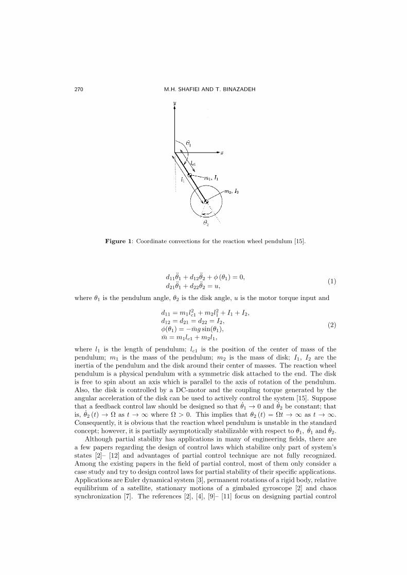
270 M.H. SHAFIEI AND T. BINAZADEH
Figure 1: Coordinate convections for the reaction wheel pendulum [15].
d11θ1 + d12θ2 + φ (θ1) = 0,
d21θ1 + d22θ2 = u,(1)
where θ1 is the pendulum angle, θ2 is the disk angle, u is the motor torque input and
d11 = m1l2c1 +m2l
21 + I1 + I2,
d12 = d21 = d22 = I2,φ(θ1) = −mg sin(θ1),m = m1lc1 +m2l1,
(2)
where l1 is the length of pendulum; lc1 is the position of the center of mass of thependulum; m1 is the mass of the pendulum; m2 is the mass of disk; I1, I2 are theinertia of the pendulum and the disk around their center of masses. The reaction wheelpendulum is a physical pendulum with a symmetric disk attached to the end. The diskis free to spin about an axis which is parallel to the axis of rotation of the pendulum.Also, the disk is controlled by a DC-motor and the coupling torque generated by theangular acceleration of the disk can be used to actively control the system [15]. Supposethat a feedback control law should be designed so that θ1 → 0 and θ2 be constant; thatis, θ2 (t) → Ω as t → ∞ where Ω > 0. This implies that θ2 (t) = Ωt → ∞ as t → ∞.Consequently, it is obvious that the reaction wheel pendulum is unstable in the standardconcept; however, it is partially asymptotically stabilizable with respect to θ1, θ1 and θ2.
Although partial stability has applications in many of engineering fields, there area few papers regarding the design of control laws which stabilize only part of system’sstates [2]– [12] and advantages of partial control technique are not fully recognized.Among the existing papers in the field of partial control, most of them only consider acase study and try to design control laws for partial stability of their specific applications.Applications are Euler dynamical system [3], permanent rotations of a rigid body, relativeequilibrium of a satellite, stationary motions of a gimbaled gyroscope [2] and chaossynchronization [7]. The references [2], [4], [9]– [11] focus on designing partial control
NONLINEAR DYNAMICS AND SYSTEMS THEORY, 12 (3) (2012) 269–277 271
and have given some way of designing. However, it is worth noting that the controlschemes posed in these references are uneasy to realize and are usable only for systemswith some special structures. In [12], a new class of nonlinear systems which is called“partially passive system” was introduced and some theorems for partial stabilizationwere developed.
In this paper, some new partial stabilization theorems for nonlinear dynamical sys-tems are posed. It is shown that partial control makes the possibility of converting thecontrol problem into a simpler one having fewer control input variables; which is one ofthe main contributions of this paper. In all of the existing papers in the field of partialcontrol, the input vector is wholly designed; but in this paper by designing the reducedinput vector, the advantage of partial control in simplifying the problem by reducingthe control variables is recognized. The system’s state is separated into two parts andaccordingly the nonlinear dynamical system is divided into two subsystems. The subsys-tems, hereafter, are referred to as the “first” and the “second” subsystems. The reducedcontrol input vector (the vector that includes components of input vector which appearin the first subsystem) is designed in such a way to guarantee asymptotic stability of thenonlinear system with respect to the first part of state vector. The design procedure isbased on selection of a proper control Lyapunov function which is called partial controlLyapunov function. It’s name is because that in this function only the first part of statesis appeared.
The remainder of this paper is arranged as follows. First, the preliminaries on partialstability/control are given in Section 2. In Section 3, the theorems for partial controldesign are presented and explained in detail. Finally, conclusions are made in Section 4.
2 Preliminaries
In this section, the definitions and notations of partial stability are introduced. Considera nonlinear system in the form;
x = f(x), x(t0) = x0, (3)
where x ∈ Rn is the state vector. Let vectors x1 and x2 denote the partitions of thestate vector, respectively. Therefore, x = (xT
1 , xT2 )
T where x1 ∈ Rn1 , x2 ∈ Rn2 andn1 + n2 = n. As a result, the nonlinear system (3) can be divided into two parts (thefirst and the second subsystems) as follows
x1(t) = F1(x1(t), x2(t)), x1(t0) = x10,x2(t) = F2(x1(t), x2(t)), x2(t0) = x20,
(4)
where x1 ∈ D ⊆ Rn1 , D is an open set including the origin, x2 ∈ Rn2 and F1 : D×Rn2 →Rn1 is such that for every x2 ∈ Rn2 , F1(0, x2) = 0 and F1(., x2) is locally Lipschitz inx1. Also, F2 : D×Rn2 → Rn2 is such that for every x1 ∈ D, F2(x1, .) is locally Lipschitzin x2, and Ix0
= [0, τx0) , 0 < τx0
≤ ∞ is the maximal interval of existence of solution(x1(t), x2(t)) of (4) ∀t ∈ Ix0
. Under these conditions, the existence and uniqueness ofsolution is ensured. Now, stability of the dynamical system (4) with respect to x1 canbe defined as follows [5]:
Definition 2.1 1. The nonlinear system (4) is Lyapunov stable with respect tox1 if for every ε > 0 and x20 ∈ Rn2 , there exists δ(ε, x20) > 0 such that ‖x10‖ < δimplies ‖x1(t)‖ < ε for all t ≥ 0.
272 M.H. SHAFIEI AND T. BINAZADEH
2. The nonlinear system (4) is asymptotically stable with respect to x1, if it is Lya-punov stable with respect to x1 and for every x20 ∈ Rn2 , there exists δ = δ(x20) > 0such that ‖x10‖ < δ implies limt→∞ x1(t) = 0.
It is important to note that this partial stability definition (which is given in [5]) isdifferent from past definitions of partial stability [1, 4]. In past definitions, it is requiredthat F1(0, 0) = 0 and F2(0, 0) = 0. Also, the initial condition of the whole system shouldbe in a neighborhood of the origin which is not required in Definition 2.1. The mainadvantage of considering the condition F1(0, x2) = 0 for every x2, is that it makes thepossibility of investigating the partial stability even if a part of system’s states goes toinfinity. Using this fact, authors of [5] present the unification of partial stability theoryfor autonomous systems and stability theory for nonlinear time-varying systems. Thisunification allows the stability theory of time-varying systems to be presented as a specialcase of autonomous partial stability theory.
In order to analyze partial stability, the following theorem and its corollary are takenfrom [5]. Note that in the following theorem, V (x1, x2) = V ′(x1, x2)F (x1, x2) where the
row vector of ∂V (x)/∂x is shown by V ′(x) and F (x1, x2) =[
FT1 (x1, x2) FT
2 (x1, x2)]T
.
Theorem 2.1 Consider the nonlinear dynamical system (4). If there exist a contin-uously differentiable function V : D×Rn2 → R and class K functions α(.) and γ(.) suchthat
V (0, x2) = 0, x2 ∈ Rn2 , (5)
α(‖x1‖) ≤ V (x1, x2), (x1, x2) ∈ D ×Rn2 , (6)
V (x1, x2) ≤ −γ(‖x1‖), (x1, x2) ∈ D ×Rn2 , (7)
then, the nonlinear dynamical system (4) is asymptotically stable with respect to x1.
Proof. See [5]. 2
Corollary 2.1 Consider the nonlinear dynamical system (4). If there exist a positivedefinite continuously differentiable function V : D → R, and a class K function γ(.) suchthat
V ′(x1)F1(x1, x2) ≤ −γ (‖x1‖) , (x1, x2) ∈ D ×Rn2 , (8)
then, the equilibrium point of the nonlinear dynamical system (4) is asymptotically stablewith respect to x1.
Now, consider the following autonomous nonlinear control system:
x1(t) = F1(x1, x2, u(x1, x2)), x1(t0) = x10,x2(t) = F2(x1, x2, u(x1, x2)), x2(t0) = x20,
(9)
where u ∈ Rm and F1 : D×Rn2 ×Rm → Rn1 is such that for every x2 ∈ Rn2 , F1(., x2, .)is locally Lipschitz in x1 and u. Also, F2 : D × Rn2 × Rm → Rn2 is such that for everyx1 ∈ D, F2(x1, ., .) is locally Lipschitz in x2 and u. These assumptions guarantee thelocal existence and uniqueness of the solution of the differential equations (9).
Definition 2.2 The nonlinear control system (9) is said to be asymptotically stabiliz-able with respect to x1, if there exists some admissible feedback control law u = k(x1, x2),which makes system (9) asymptotically stable with respect to x1.
NONLINEAR DYNAMICS AND SYSTEMS THEORY, 12 (3) (2012) 269–277 273
3 An Approach for Partial Control Design
This section presents a feasible design algorithm for partial stabilization of nonlinearsystems. Suppose the x1-subsystem in Eq. (9) is affine with respect to the control input(the x2-equation may have a general dynamical form). Therefore,
x1 = f1(x1, x2) +∑m
i=1 g1i(x1, x2)ui,
x2(t) = F2(x1, x2, u),(10)
where ui is the ith component of input vector u. Also, g1i ∈ Rn1 , for i=1,2,. . . ,m. Letdefine r = number of (g1i 6= 0)i=1,...,m. Hence, r is the number of components of inputvector which appear in x1-subsystem. Thus 0 ≤ r ≤ m. Now, with respect to the valueof r, two cases may be considered.
3.1 Case 1: r 6= 0
By augmenting the r nonzero vectors g1i in a matrix, the nonlinear system (10) can berewritten as follows;
x1 = f1(x1, x2) +G1(x1, x2)u1,x2 = F2(x1, x2, u),
(11)
where u1 ∈ Rr is the reduced version of input vector u, that contains r control variablesappearing in x1-subsystem, G1(x1, x2) is an n1 × r matrix where its columns are the rnonzero vectors g1i. In this case, the task is to find an appropriate u1, which guaranteespartial stabilization of nonlinear system (11) with respect to x1.
Theorem 3.1 Consider the nonlinear dynamical system (11). Suppose V (x1) : D →R is a positive definite continuously differentiable function (which is called partial controlLyapunov function) with the property that no solution x1 of the unforced system (11) canstay identically in the set V ′(x1) = 0 other than the trivial solution x1(t) ≡ 0. Also,suppose γ(.) is class K function. Then, the system may be asymptotically stabilizablewith respect to x1 through the following reduced input vector
u1 = k1(x1, x2) =
bT−V ′(x1)f1−γ(‖x1‖)bbT
, where bbT 6= 0,0, where bbT = 0,
(12)
where b = V ′(x1)G1(x1, x2). It is stressed that only in the points of state space x1 − x2
where bbT = 0, the following condition should be satisfied:
V ′(x1)f1(x1, x2) = −γ (‖x1‖) ∀(x1, x2), where bbT = 0. (13)
Proof. By use of the control law (12), the time derivative of V (x1) in the line ofsystem’s trajectory is
V (x1) = V ′(x1)x1
= V ′(x1)f1 + V ′(x1)G1
[
(V ′(x1)G1)T−V ′(x1)f1−γ(‖x1‖)
(V ′(x1)G1)(V ′(x1)G1)T
]
(14)
=V ′(x1)f1 + −V ′(x1)f1 − γ (‖x1‖)= −γ (‖x1‖).
274 M.H. SHAFIEI AND T. BINAZADEH
Therefore, according to Corollary 2.1, the nonlinear system (11) is asymptoticallystable with respect to x1. For the case where bbT = 0, if condition (13) is satisfied, thenby taking u1 = 0, partial stability will be achieved. 2
Note: When V ′(x1) = 0, then bbT = 0. In the points where bbT = 0, condition(13) should be satisfied, which results in γ (‖x1‖) = 0. Since, γ (.) is a class K function,thus γ (‖x1‖) = 0 ⇒ x1 = 0. Therefore, as mentioned in Theorem 3.1, V (x1) should bechosen in a way that V ′(x1) = 0 ⇒ x1 ≡ 0.
3.2 Case 2: r = 0
This situation means that there is no component of input vector in x1-subsystem. Sup-pose that x2-subsystem is affine with respect to input. Therefore,
x1 = f1(x1, x2),x2 = f2(x1, x2) +G2(x1, x2)u.
(15)
This system may be viewed as a cascade connection of two subsystems where x2 isto be viewed as an input for first subsystem. The form (15) is usually referred to asthe regular form. Assume that x2 and u both belong to Rm (in other words, n2 = m),and G2(x1, x2) is an m by m nonsingular matrix. This assumption is not so restrictiveand many design methods, which are based on regular forms, e.g., backstepping or slid-ing mode techniques use such an assumption [16]. In this case, the task is to find anappropriate u; which guarantees partial stabilization of the closed-loop system.
Theorem 3.2 Consider the nonlinear dynamical system (15). Suppose V (x1) : D →R is a partial control Lyapunov function, γ(.) is a class K function and ϕ(x1) is a smoothfunction. The design of the function ϕ(x1) is such that
V ′(x1)(f1(x1, ϕ(x1))) ≤ −γ(‖x1‖). (16)
Therefore, the nonlinear system (15) may be asymptotically stabilized with respect to x1
by the following input vector
u =G−12 [ϕ′(x1)f1 − f2]. (17)
Proof. Substitution of (17) in x2-subsystem (15) yields,
x2 = f2 +G2u= f2 +G2G
−12 [ϕ′(x1)f1 − f2]
= ϕ′(x1)f1
(18)
which results in x2 = ϕ(x1). Since the condition (16) means that the first subsystem (x1-subsystem) may be asymptotically stabilized by a virtual input in the form x2 = ϕ(x1)(according to Corollary 2.1). Therefore, the control law (17) partially stabilized thenonlinear system (15) with respect to x1. 2
3.3 Example. Partial stabilization of reaction wheel pendulum
The reaction wheel pendulum was described in Introduction. We define the states z1 =θ1, z2 = θ1, z3 = θ2 and z4 = θ2, The system’s equations (1) can be written as follows
z1 = z2,
z2 = − d22
detDφ(z1)− d12
detDu,z3 = z4,
z4 =d21
detDφ(z1) +d11
detDu,
(19)
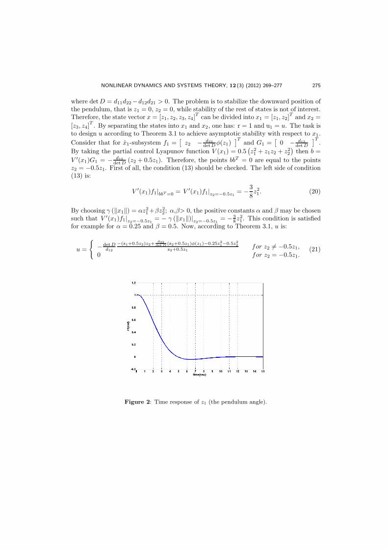
NONLINEAR DYNAMICS AND SYSTEMS THEORY, 12 (3) (2012) 269–277 275
where detD = d11d22−d12d21 > 0. The problem is to stabilize the downward position ofthe pendulum, that is z1 = 0, z2 = 0, while stability of the rest of states is not of interest.Therefore, the state vector x = [z1, z2, z3, z4]
Tcan be divided into x1 = [z1, z2]
Tand x2 =
[z3, z4]T. By separating the states into x1 and x2, one has: r = 1 and u1 = u. The task is
to design u according to Theorem 3.1 to achieve asymptotic stability with respect to x1.
Consider that for x1-subsystem f1 =[
z2 − d22
detDφ(z1)]T
and G1 =[
0 − d12
detD
]T.
By taking the partial control Lyapunov function V (x1) = 0.5(
z21 + z1z2 + z22)
then b =
V ′(x1)G1 = − d12
detD (z2 + 0.5z1). Therefore, the points bbT = 0 are equal to the pointsz2 = −0.5z1. First of all, the condition (13) should be checked. The left side of condition(13) is:
V ′(x1)f1|bbT=0 = V ′(x1)f1|z2=−0.5z1= −3
8z21 . (20)
By choosing γ (‖x1‖) = αz21+βz22 ; α,β> 0, the positive constants α and β may be chosensuch that V ′(x1)f1|z2=−0.5z1
= − γ (‖x1‖)|z2=−0.5z1= − 3
8z21 . This condition is satisfied
for example for α = 0.25 and β = 0.5. Now, according to Theorem 3.1, u is:
u =
−detDd12
−(z1+0.5z2)z2+d22
det D(z2+0.5z1)φ(z1)−0.25z2
1−0.5z2
2
z2+0.5z1for z2 6= −0.5z1,
0 for z2 = −0.5z1.(21)
Figure 2: Time response of z1 (the pendulum angle).
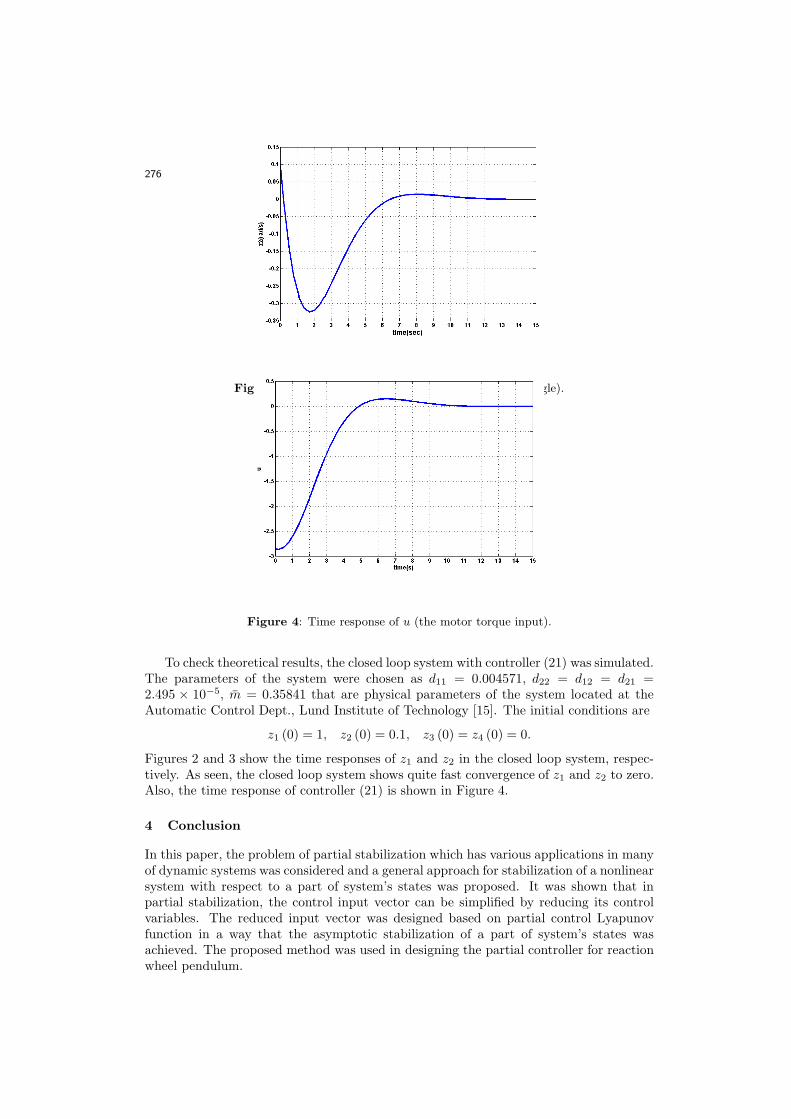
276 M.H. SHAFIEI AND T. BINAZADEH
Figure 3: Time response of z2 (rate of the pendulum angle).
Figure 4: Time response of u (the motor torque input).
To check theoretical results, the closed loop system with controller (21) was simulated.The parameters of the system were chosen as d11 = 0.004571, d22 = d12 = d21 =2.495 × 10⁻⁵, m = 0.35841 that are physical parameters of the system located at theAutomatic Control Dept., Lund Institute of Technology [15]. The initial conditions are
z1 (0) = 1, z2 (0) = 0.1, z3 (0) = z4 (0) = 0.
Figures 2 and 3 show the time responses of z1 and z2 in the closed loop system, respec-tively. As seen, the closed loop system shows quite fast convergence of z1 and z2 to zero.Also, the time response of controller (21) is shown in Figure 4.
4 Conclusion
In this paper, the problem of partial stabilization which has various applications in manyof dynamic systems was considered and a general approach for stabilization of a nonlinearsystem with respect to a part of system’s states was proposed. It was shown that inpartial stabilization, the control input vector can be simplified by reducing its controlvariables. The reduced input vector was designed based on partial control Lyapunovfunction in a way that the asymptotic stabilization of a part of system’s states wasachieved. The proposed method was used in designing the partial controller for reactionwheel pendulum.
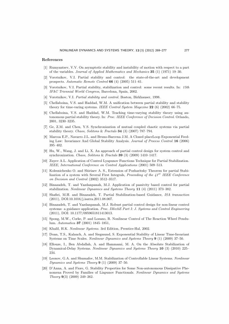
NONLINEAR DYNAMICS AND SYSTEMS THEORY, 12 (3) (2012) 269–277 277
References
[1] Rumyantsev, V.V. On asymptotic stability and instability of motion with respect to a partof the variables. Journal of Applied Mathematics and Mechanics 35 (1) (1971) 19–30.
[2] Vorotnikov, V.I. Partial stability and control: the state-of-the-art and developmentprospects. Automatic Remote Control 66 (4) (2005) 511–61.
[3] Vorotnikov, V.I. Partial stability, stabilization and control: some recent results. In: 15thIFAC Triennial World Congress, Barcelona, Spain, 2002.
[4] Vorotnikov, V.I. Partial stability and control. Boston, Birkhauser, 1998.
[5] Chellaboina, V.S. and Haddad, W.M. A unification between partial stability and stabilitytheory for time-varing systems. IEEE Control System Magezine 22 (6) (2002) 66–75.
[6] Chellaboina, V.S. and Haddad, W.M. Teaching time-varying stability theory using au-tonomous partial stability theory. In: Proc. IEEE Conference of Decision Control. Orlando,2001, 3230–3235.
[7] Ge, Z.M. and Chen, Y.S. Synchronization of mutual coupled chaotic systems via partialstability theory. Chaos, Solitons & Fractals 34 (3) (2007) 787–794.
[8] Marcoa E.P., Navarro J.L. and Bruno-Barcena J.M. A Closed placeLoop Exponential Feed-ing Law: Invariance And Global Stability Analysis. Journal of Process Control 16 (2006)395–402.
[9] Hu, W., Wang, J. and Li, X. An approach of partial control design for system control andsynchronization. Chaos, Solitons & Fractals 39 (3) (2009) 1410–1417.
[10] Zuyev A.L. Application of Control Lyapunov Functions Technique for Partial Stabilization.IEEE, International Conference on Control Applications (2001) 509–513.
[11] Kolesnichenko O. and Shiriaev A. S., Extension of Pozharitsky Theorem for partial Stabi-lization of a system with Several First Integrals, Proceeding of the 41st IEEE Conferenceon Decision and Control (2002) 3512–3517.
[12] Binazadeh, T. and Yazdanpanah, M.J. Application of passivity based control for partialstabilization. Nonlinear Dynamics and Systems Theory 11 (4) (2011) 373–382.
[13] Shafiei, M.H. and Binazadeh, T. Partial Stabilization-based Guidance, ISA transaction(2011), DOI:10.1016/j.isatra.2011.08.007.
[14] Binazadeh, T. and Yazdanpanah, M.J. Robust partial control design for non-linear controlsystems: a guidance application. Proc. IMechE Part I: J. Systems and Control Engineering(2011), DOI: 10.1177/0959651811413013.
[15] Spong, M.W., Corke, P. and Lozano, R. Nonlinear Control of The Reaction Wheel Pendu-lum. Automatica 37 (2001) 1845–1851,
[16] Khalil, H.K. Nonlinear Systems. 3rd Edition, Prentice-Hal, 2002.
[17] Doan, T.S., Kalauch, A. and Siegmund, S. Exponential Stability of Linear Time-InvariantSystems on Time Scales. Nonlinear Dynamics and Systems Theory 9 (1) (2009) 37–50.
[18] Ellouze, I., Ben Abdallah, A. and Hammami, M. A. On the Absolute Stabilization ofDynamical-Delay Systems. Nonlinear Dynamics and Systems Theory 10 (3) (2010) 225–234.
[19] Leonov, G.A. and Shumafov, M.M. Stabilization of Controllable Linear Systems. NonlinearDynamics and Systems Theory 9 (1) (2009) 37–50.
[20] D’Anna, A. and Fiore, G. Stability Properties for Some Non-autonomous Dissipative Phe-nomena Proved by Families of Liapunov Functionals. Nonlinear Dynamics and SystemsTheory 9(3) (2009) 249–262.

Nonlinear Dynamics and Systems Theory, 12 (3) (2012) 279–287
Wavelet Neural Network Based Adaptive Tracking
Control for a Class of Uncertain Nonlinear Systems
Using Reinforcement Learning
M. Sharma 1∗ and A. Verma 2
1 MediCaps Institute of Tech. and Mgmt., Indore, India2 Institute of Engineering and Technology, Indore, India
Received: May 6, 2011; Revised: March 5, 2012
Abstract: In this paper an adaptive critic based wavelet neural network (WNN)based tracking control strategy for a class of uncertain systems in continous time isproposed. The adaptive critic WNN controller comprises two WNNs: critic WNNand action WNN. The critic WNN is approximating the strategic utility function,whereas the action WNN is minimizing both the strategic utility function and theunknown nonlinear dynamic estimation errors. Adaptation laws are developed forthe online tuning of wavelets parameters. The uniformly ultimate boundedness ofthe closed-loop tracking error is verified even in the presence of WNN approximationerrors and bounded unknown disturbances, using the Lyapunov approach and withnovel weight updating rules. Finally some simulations are performed to verify theeffectiveness and performance of the theoretical development.
Keywords: wavelet neural networks; optimal control; adaptive control; reinforce-ment learning; Lyapunov functional.
1 Introduction
Typical control strategies are based on a mathematical model that captures as muchinformation as possible about the plant to be controlled. The ultimate objective is not todesign the best controller for the plant model, but for the real time plant. This objectiveis addressed by robust control theory by including in the model a set of uncertainties.Robust control techniques are applied to the plant model, augmented with uncertaintiesand candidate controllers, to analyze the stability of the actual system. This is a powerful
∗ Corresponding author: mailto:[email protected]
c© 2012 InforMath Publishing Group/1562-8353 (print)/1813-7385 (online)/http://e-ndst.kiev.ua 279
280 M. SHARMA AND A. VERMA
tool for practical controller design, but designing a controller that remains stable in thepresence of uncertainties limits the aggressiveness of the resulting controller, and canresult in suboptimal control performance [1, 2].
In this paper, the robust control techniques are combined with a reinforcement learn-ing algorithm to improve the performance of robust controller while maintaining thestability of the system. Reinforcement learning is a class of algorithms for solving multi-step, sequential decision problems by finding a policy for choosing sequences of actionsthat optimize the sum of some performance criterion over time [3]– [7].
In recent years, learning-based control methodology using Neural networks (NNs)has become an alternative to adaptive control since NNs are considered as general toolsfor modeling nonlinear systems [17]. Work on adaptive NN control using the universalNN approximation property is now pursued by several groups of researchers. By usingneural network (NN) as an approximation tool, the assumptions on linear parameterizednonlinearities in adaptive controller designing aspects have greatly been relaxed. It alsobroadens the class of the uncertain nonlinear systems which can be effectively dealt byadaptive controllers. However there are some difficulties associated with NN based con-troller. The basis functions are generally not orthogonal or redundant; i.e., the networkrepresentation is not unique and is probably not the most efficient one and the conver-gence of neural networks may not be guaranteed. Also the training procedure for NNmay be trapped in some local minima depending on the initial settings. Wavelet neuralnetworks are the modified form of the NN having the properties of space and frequencylocalization properties leading to a superior learning capabilities and fast convergence.Thus WNN based control systems can achieve better control performance than NN basedcontrol systems [8]– [10].
Adaptive actor-critic WNN-based control has emerged as a promising WNN approachdue to its potential to find approximate solutions to dynamic programming [11]– [14].In the actor-critic WNN based control a long-term system performance measure can beoptimized, in contrast to the short-term performance measure used in classical adaptiveand WNN control. While the role of the actor is to select actions, the role of thecritic is to evaluate the performance of the actor. This evaluation is used to providethe actor with a signal that allows it to improve its performance, typically by updatingits parameters along an estimate of the gradient of some measure of performance, withrespect to the actor’s parameters. The critic WNN approximates a certain strategicsutility function that is similar to a standard Bellman equation, which is taken as thelong-term performance measure of the system. The weights of action WNN are tunedonline by both the critic WNN signal and the filtered tracking error. It minimizes thestrategic utility function and uncertain system dynamic estimation errors so that theoptimal control signal can be generated [3].
This paper deals with the designing of reinforcement learning WNN based adaptivetracking controller for a class of uncertain nonlinear systems. WNN are used for approx-imating the system uncertainty as well as to optimize the performance of the controlstrategy.
The paper is organized as follows. Section 2 deals with the system preliminaries,system description is given in Section 3. WNN based controller designing aspects arediscussed in Section 4. Section 5 describes the tuning algorithm for actor-critic wavelets.The stability analysis of the proposed control scheme is given in Section 6. Effectivenessof the proposed strategy is illustrated through an example in Section 7 while Section 8concludes the paper.
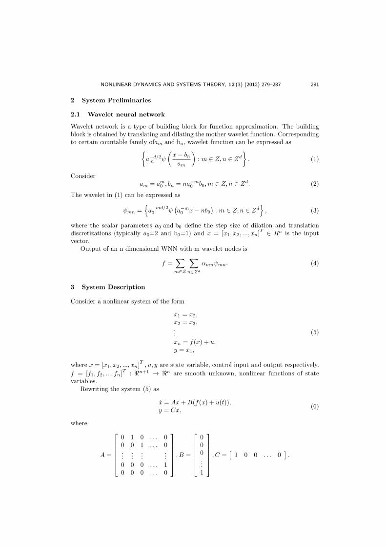
NONLINEAR DYNAMICS AND SYSTEMS THEORY, 12 (3) (2012) 279–287 281
2 System Preliminaries
2.1 Wavelet neural network
Wavelet network is a type of building block for function approximation. The buildingblock is obtained by translating and dilating the mother wavelet function. Correspondingto certain countable family ofam and bn, wavelet function can be expressed as
a−d/2m ψ
(x− bnam
): m ∈ Z, n ∈ Zd
. (1)
Consideram = am0 , bn = na−m0 b0,m ∈ Z, n ∈ Zd. (2)
The wavelet in (1) can be expressed as
ψmn =a−md/20 ψ
(a−m0 x− nb0
): m ∈ Z, n ∈ Zd
, (3)
where the scalar parameters a0 and b0 define the step size of dilation and translationdiscretizations (typically a0=2 and b0=1) and x = [x1, x2, ..., xn]
T ∈ Rn is the inputvector.
Output of an n dimensional WNN with m wavelet nodes is
f =∑m∈Z
∑n∈Zd
αmnψmn. (4)
3 System Description
Consider a nonlinear system of the form
x1 = x2,x2 = x3,...xn = f(x) + u,y = x1,
(5)
where x = [x1, x2, ..., xn]T, u, y are state variable, control input and output respectively.
f = [f1, f2, ..., fn]T
: <n+1 → <n are smooth unknown, nonlinear functions of statevariables.
Rewriting the system (5) as
x = Ax+B(f(x) + u(t)),y = Cx,
(6)
where
A =
0 1 0 . . . 00 0 1 . . . 0...
......
...0 0 0 . . . 10 0 0 . . . 0
, B =
000...1
, C =[
1 0 0 . . . 0].
282 M. SHARMA AND A. VERMA
The objective is to formulate a state feedback control law to achieve the desiredtracking performance. The control law is formulated using the transformed system (6).
Let yd = [yd, yd, . . . ,n−1yd ]T be the vector of desired tracking trajectory. The following
assumptions are taken for the systems under consideration.
Assumption 3.1 Desired trajectory yd (t) is assumed to be smooth, continuous Cn
and available for measurement.
4 Basic Controller Design Using Filtered Tracking Error
Define the state tracking error vector e(t) as
e(t) = x(t)− yd(t). (7)
The filter tracking error is defined as
r = Ke,
where K = [k1, k2, . . . kn−1, 1] is an appropriately chosen coefficient vector such thate→ 0 exponentially as < → 0. Differentiating it along the trajectory of the systems, weget
˙r = Kee+ f(x) + u− nyd . (8)
Applying the feedback linearization method, the control law is defined as
u = (nyd−f(x)−Kee− r), (9)
where Ke = [0, k1, k2, . . . , kn−1]. Substituting (9) in (8),
˙r = −r + f(x). (10)
Stability of the system (6) with the proposed control strategy will be analyzed in thesubsequent section.
5 Adaptive WNN Controller Design
A novel strategic utility function is defined as the long-term performance measure forthe system. It is approximated by the WNN critic signal. The action WNN signal isconstructed to minimize this strategic utility function by using a quadratic optimizationfunction. The critic WNN and action WNN weight tuning laws are derived. Stabilityanalysis using the Lyapunov direct method is carried out for the closed-loop system (6)with novel weight tuning updates.
5.1 Strategic utility function
The utility function p(k) = [pi(k)]mi=1 ∈ <m is defined on the basis of the filtered trackingerror r and is given by [3]:
pi(k) = 0, if r2i ≤ η,pi(k) = 1, if r2i> η,
(11)
NONLINEAR DYNAMICS AND SYSTEMS THEORY, 12 (3) (2012) 279–287 283
where pi(k) ∈ <, i = 1, 2, . . . ,m and η ∈ < is the predefined threshold, p(k) can beconsidered as the current performance index. The long term system performance measureQ′(k) ∈ <m can be defined using the binary utility function as
Q′(k) = αNp(k + 1) + αN−1p(k + 2) + . . .+ αk+1p(N) + . . . , (12)
where α ∈ < and 0 <α< 1 and N is the horizon. Above equation may be rewritten as
Q(k) = minu(k)αQ(k − 1)− αN+1p(k).
This measure is similar to standard Bellman’s equation [15].
5.1.1 Critic WNN
Q′(k)is approximated by the critic WNN by defining the prediction error as
ec(k) = Q(k)− α(Q(k − 1)− αNp(k)), (13)
where Q(k) = wT1 (k)φ1(vT1 x(k)) = wT1 (k)φ1(k), ec(k) ∈ <m, Q(k) ∈ <m is the criticsignal, w1(k) ∈ <n1×m and v1 ∈ <nm×n1 represent the weight estimates, φ1(k) ∈ <n1isthe wavelet activation function and n1 is the number of nodes in the wavelet layer. Theobjective function to be minimized by the critic NN is defined as:
Ec(k) =1
2eTc (k)ec(k). (14)
The weight update rule for the critic NN is a gradient-based adaptation, which is givenby [3]
w1(k + 1) = w1(k) + ∆w1(k),
where
∆w1(k) = α1
[−∂Ec(k)
∂w1(k)
](15)
or
w1(k + 1) = w1(k)− α1φ1(k)×(wT1 (k)φ1(k) + αN+1p(k)− αwT1 (k − 1)φ1(k − 1))T ,(16)
where α1 ∈ < is the WNN adaptation gain. The critic WNN weights are tuned by thereinforcement learning signal and discounted values of critic WNN past outputs.
5.1.2 Action WNN
The output of the action NN is to approximate the unknown nonlinear function f(x(k))and to provide an optimal control signal to be the part of the overall input u(k) as
f(k) = wT2 (k)φ2(vT2 x(k)) = wT2 (k)φ2(k), (17)
where w2(k) ∈ <n2×m and v2 ∈ <nm×n2 represent the matrix of weight estimate, φ2(k) ∈<n2 is the activation function, n2 is the number of nodes in the hidden layer. Supposethat the unknown target output-layer weight for the action WNN is w2 then we have
f(k) = wT2 (k)φ2(vT2 x(k))ε2(x(k)) = wT2 (k)φ2(k)ε2(x(k)), (18)
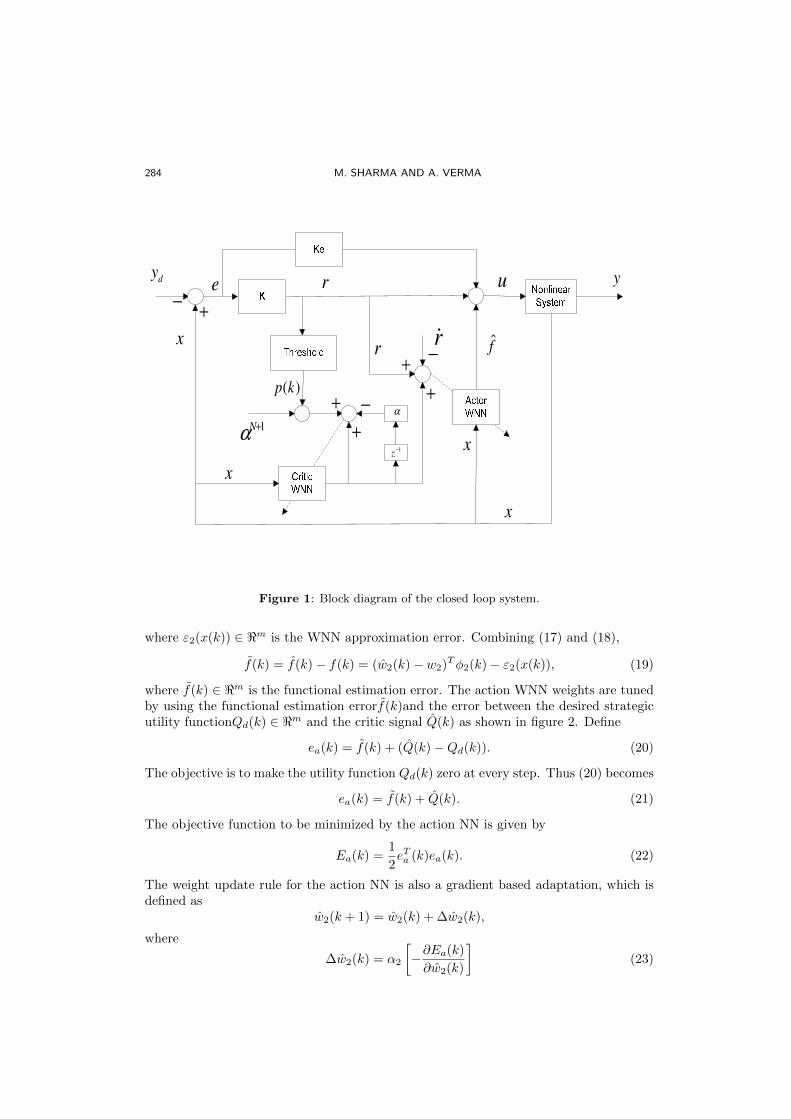
284 M. SHARMA AND A. VERMA
e
x
f
dy u y
+−
r
1z
−
α
x
x
x
( )p k
1Nα
++
−+
+
+
−r
r
Figure 1: Block diagram of the closed loop system.
where ε2(x(k)) ∈ <m is the WNN approximation error. Combining (17) and (18),
f(k) = f(k)− f(k) = (w2(k)− w2)Tφ2(k)− ε2(x(k)), (19)
where f(k) ∈ <m is the functional estimation error. The action WNN weights are tunedby using the functional estimation errorf(k)and the error between the desired strategicutility functionQd(k) ∈ <m and the critic signal Q(k) as shown in figure 2. Define
ea(k) = f(k) + (Q(k)−Qd(k)). (20)
The objective is to make the utility function Qd(k) zero at every step. Thus (20) becomes
ea(k) = f(k) + Q(k). (21)
The objective function to be minimized by the action NN is given by
Ea(k) =1
2eTa (k)ea(k). (22)
The weight update rule for the action NN is also a gradient based adaptation, which isdefined as
w2(k + 1) = w2(k) + ∆w2(k),
where
∆w2(k) = α2
[−∂Ea(k)
∂w2(k)
](23)
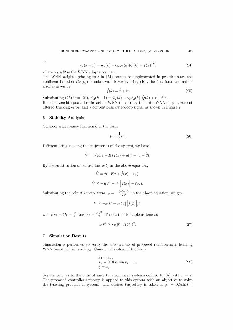
NONLINEAR DYNAMICS AND SYSTEMS THEORY, 12 (3) (2012) 279–287 285
orw2(k + 1) = w2(k)− α2φ2(k)(Q(k) + f(k))T , (24)
where α2 ∈ < is the WNN adaptation gain.The WNN weight updating rule in (24) cannot be implemented in practice since thenonlinear function f(x(k)) is unknown. However, using (10), the functional estimationerror is given by
f(k) = ˙r + r. (25)
Substituting (25) into (24), w2(k + 1) = w2(k)− α2φ2(k)(Q(k) + ˙r − r)T .Here the weight update for the action WNN is tuned by the critic WNN output, currentfiltered tracking error, and a conventional outer-loop signal as shown in Figure 2.
6 Stability Analysis
Consider a Lyapunov functional of the form
V =1
2r2. (26)
Differentiating it along the trajectories of the system, we have
V = r(Kee+K(f(x) + u(t)− vr −nyd).
By the substitution of control law u(t) in the above equation,
V = r(−Kr + f(x)− vr).
V ≤ −Kr2 + |r|∣∣∣f(x)
∣∣∣− rvr).Substituting the robust control term vr = − (ρ2+1)r
2ρ2 in the above equation, we get
V ≤ −s1r2 + s2(|r|∣∣∣f(x)
∣∣∣)2,where s1 = (K + K
2 ) and s2 =Kρ2
2 . The system is stable as long as
s1r2 ≥ s2(|r|
∣∣∣f(x)∣∣∣)2. (27)
7 Simulation Results
Simulation is performed to verify the effectiveness of proposed reinforcement learningWNN based control strategy. Consider a system of the form
x1 = x2,x2 = 0.01x1 sinx2 + u,y = x1.
(28)
System belongs to the class of uncertain nonlinear systems defined by (5) with n = 2.The proposed controller strategy is applied to this system with an objective to solvethe tracking problem of system. The desired trajectory is taken as yd = 0.5 sin t +
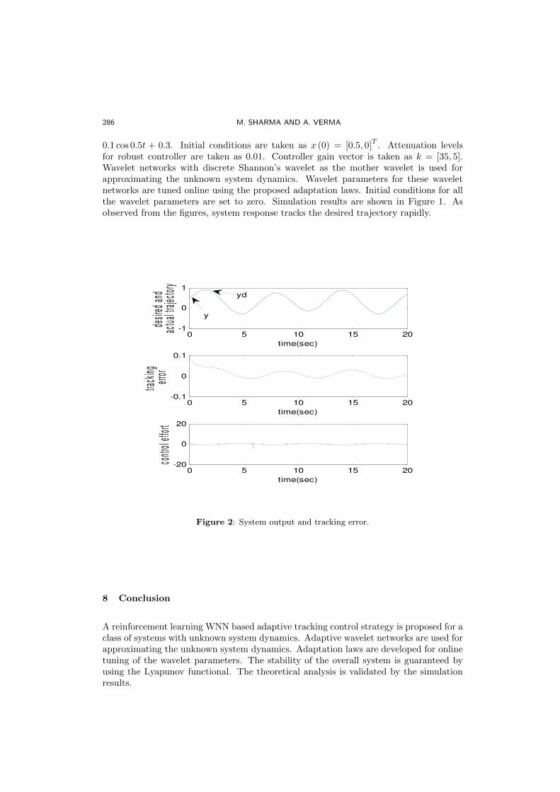
286 M. SHARMA AND A. VERMA
0.1 cos 0.5t + 0.3. Initial conditions are taken as x (0) = [0.5, 0]T
. Attenuation levelsfor robust controller are taken as 0.01. Controller gain vector is taken as k = [35, 5].Wavelet networks with discrete Shannon’s wavelet as the mother wavelet is used forapproximating the unknown system dynamics. Wavelet parameters for these waveletnetworks are tuned online using the proposed adaptation laws. Initial conditions for allthe wavelet parameters are set to zero. Simulation results are shown in Figure 1. Asobserved from the figures, system response tracks the desired trajectory rapidly.
0 5 10 15 20-1
0
1
time(sec)
desir
ed an
d ac
tual tr
ajecto
ry
0 5 10 15 20-0.1
0
0.1
time(sec)
track
ing
error
0 5 10 15 20-20
0
20
time(sec)
contr
ol eff
ort
y
yd
Figure 2: System output and tracking error.
8 Conclusion
A reinforcement learning WNN based adaptive tracking control strategy is proposed for aclass of systems with unknown system dynamics. Adaptive wavelet networks are used forapproximating the unknown system dynamics. Adaptation laws are developed for onlinetuning of the wavelet parameters. The stability of the overall system is guaranteed byusing the Lyapunov functional. The theoretical analysis is validated by the simulationresults.
NONLINEAR DYNAMICS AND SYSTEMS THEORY, 12 (3) (2012) 279–287 287
References
[1] Wen, J. W. and Liu, F. Robust Model Predictive Control for Fuzzy Systems Subject toActuator Saturation. In: Sixth International Conference on Fuzzy Systems and KnowledgeDiscovery (2009) 400–404.
[2] Chen, J. and Liu, F. Robust fuzzy control for nonlinear system with disk pole constraints.Control and Decision (2007) 983–988.
[3] He, P. and Jagannathan, S. Reinforcement learning neural-network-based controller fornonlinear discrete-time systems with input constraints. IEEE Transactions on Systems,Man, and Cybernetics. Part B: Cybernetics 37(2) (2007) 425–436.
[4] Lin, W.S., Chang, L.H. and Yang, P.C. Adaptive critic anti-slip control of wheeled au-tonomous robot. IET Control Theory Applications 1(1) 2007.
[5] Crespo, L.G. Optimal performance, robustness and reliability base designs of systems withstructured uncertainty. In: Proceeding of American Control Conference (2003) 4219–4224.
[6] Zadeh, N., Jamali, N. and Hajiloo, A. Frequency-based reliability Pareto optimum designof proportional-integral-derivative controllers for systems with probabilistic uncertainty.Journal of Systems and Control Engineering (IMECHE) 22(18) (2007) 1061–1066.
[7] Peters, J. and Schaal, S. Policy gradient methods for robotics. In: Proc. of the IEEEInternational Conference on Intelligent Robotics Systems (IROS) (2006) 2219–2225.
[8] Sharma, M., Kulkarni, A. and Puntambekar, S. Wavelet based adaptive tracking controlfor uncertain nonlinear systems with input constraints. In: Proc. of the IEEE InternationalConference on advances in recent technoiogies in communication and computing (ART-COM’09) (2009) 694–698.
[9] Zhang, Q. and Benveniste, A. Wavelet networks. IEEE Transactions on Neural Networks3(6) (1992) 889–898.
[10] Zhang, J., Walter, G.G., Miao, Y. and Lee, W. Wavelet neural networks for functionlearning. IEEE Transactions on Signal Processing 43(6) (1995) 1485–1497.
[11] Jaddu, H. and Hiraishi, K. A Wavelet Approach for Solving linear quadratic optimal controlproblems. SICE-ICASE International Joint Conference (2006) 18–21.
[12] Minu, K. K., Lineesh, M. C. and John, C.J. Wavelet Neural Networks for Nonlinear TimeSeries Analysis. Applied Mathematical Sciences 4(2010) 2485–2495.
[13] Lin, X. and Balakrishnan, S. N. Convergence analysis of adaptive critic based optimalcontrol. In: Proc. of the American Control Conference (2000) 1929–1933.
[14] Murray, J. J., Cox, C., Lendaris, G.G. and Saeks, R. Adaptive dynamic programming.IEEE Transactions on System, Man, Cybernatics 32(2) (2002) 140–153.
[15] Prokhorov, D. V. and Wunsch, D.C. Adaptive critic design. IEEE Transactions on NeuralNetworks 8(5) (1997) 997–1007.
[16] Hasselt, H. V. and Wiering, D.C. Reinforcement learning in continous action space. IEEEsymposium on approximate dynamic programming and reinforcement learning (2007) 272–279.
[17] Talmoudi, S., Abderrahim, K., Abdennour, R.B. and Ksouri, M. Multimodal approach us-ing neural networks for complex systems modelling and identification. Nonlinear Dynamicsand Systems Theory 8(3) (2008) 299–316.

Nonlinear Dynamics and Systems Theory, 12 (3) (2012) 289–302
Sum of Linear Ratios Multiobjective Programming
Problem: A Fuzzy Goal Programming Approach
Pitam Singh 1 and D. Dutta 2∗
1 Department of Mathematics, Motilal Nehru National Institute of Technology,Allahabad, India
2 Department of Mathematics, National Institute of Technology,Warangal, India
Received: August 30, 2011; Revised: July 11, 2012
Abstract: Sum of ratios optimization is an interesting field of research. This pa-per presents a solution method for sum of linear ratios multiobjective programming(SOLR – MOP) problem using the fuzzy goal programming technique. Each member-ship function of fuzzy objectives is approximated into linear function by using firstorder Taylor’s theorem about the vertex of the feasible region where the objectivefunction has maximum value. Then the resulted approximated linearized member-ship functions may be used for the formulation of fuzzy goal programming. So theproblem is solved using fuzzy goal programming technique. The efficiency of themethod is measured by numerical examples.
Keywords: multiobjective programming; fractional programming; fuzzy multiobjec-tive fractional programming; sum of ratio fractional program; fuzzy goal programming.
Mathematics Subject Classification (2010): 90C29, 90C32.
1 Introduction
Ratio criteria are used to measure the efficiency of a system in any different fields ofengineering and management sciences. The ratio optimization problem is called thefractional programming. These may be applied to different disciplines such as financialsector, inventory management, production planning, banking sector and others. Ba-sically it is used for modeling real life problems with one or more objectives such asdebt/equity, profit/cost, inventory/sales, actual cost/standard cost, output/employees,nurses/patients ratios etc. with respect to some constraints.
∗ Corresponding author: mailto:[email protected]
c© 2012 InforMath Publishing Group/1562-8353 (print)/1813-7385 (online)/http://e-ndst.kiev.ua289
290 P. SINGH AND D. DUTTA
The ratio optimization problem with linear functions and linear constraints is calledlinear fractional programming (LFP) problem. If these problems have more than oneobjective then the problem is known as multiobjective linear fractional programming(MOLFP) problem.
If the ratio optimization problem has sum of linear ratios (ratios of affine functions),then the fractional programming problem (LFP) is known as sum of linear ratios pro-gramming (SOLR-P) problem.
A general sum of linear ratios programming (SOLR-P) problem is defined in thefollowing way:
Max F (x) = Max
p∑
j
fj(x)
mj(x)
= Max
p∑
j
cT0jx+ α0j
dT0jx+ β0j
subject to
x ∈ S, x ≥ 0, (1)
where p ≥ 2, x, c0j , d0j ∈ Rn, α0j , β0j ∈ R.
The feasible region S is a nonempty, compact, convex set in Rn. The function fj(x) =cT0jx + α0j , and mj(x) = dT0jx + β0j are positive for all x ∈ S. Note that under theseassumptions, the global maximum for problem (1) is attained by at least one point in S.
If we take more than one objectives in problem (1), then the problem is known as sumof linear ratios multiobjective programming (SOLR-MOP) problem, mathematically itcan be written as:
MaxF (x) = [F1(x), F2(x), . . . Fk(x)],where
Fi(x) =
p∑
j
fij(x)
mij(x), (2)
x ∈ S, x ≥ 0, p ≥ 2, x, cij , dij ∈ Rn, αij , βij ∈ R.
and fij(x) = cTijx + αij , mij(x) = dTijx + βij are positive for all x ∈ S, where S =x : Ax (≤, =, ≥) b, x ≥ 0, x ∈ Rn, b ∈ Rm, A ∈ Rm×n, (i = 1, 2, . . . , k, j =1, 2, . . . , p)∀ x ∈ S. Here, S is assumed to be non-empty compact convex set in Rn andall Fi(x) having continuous partial derivative in the feasible region S.
Sum of ratios fractional program was one of the least researched fractional programuntil about 1990. During last decade, interest in these programs has become especiallystrong. This is because, from a practical point of view, the sum of ratios fractional pro-grams have numerous applications in the fields as discussed above but still multiobjectivesum of ratios problem has least attention.
Various solution approaches have been proposed in the literature for sum of ratiosfractional program. In [6], Cambini et. al. proposed a simplex type finite algorithm forthe case p = 2 in problem (1) and find the global optimal solution. Later, Konno et.al.[13] proposed a finite parametric simplex type algorithm for the solution of linear sumof fractional programs. They give the minimization of the sum of two ratios.
In [4], Benson presented a branch- and - bound algorithm for globally solving thenonlinear sum of ratios problem. The algorithm has reduced the computational diffi-culty by conducting branch - and - bound search in Rp space rather than Rn space andthe algorithm is applied in numerical examples for verification. Benson [3] proposeda branch - and - bound algorithm using the concave envelopes for the same problem.
NONLINEAR DYNAMICS AND SYSTEMS THEORY, 12 (3) (2012) 289–302 291
In the algorithm, upper bounds are computed by maximizing concave envelopes of asum of ratios function over intersection of the feasible region of the equivalent problemwith rectangular sets systematically subdivided as branch and bound search procedure.The convergence of the algorithm is also presented and computational advantage is alsohighlighted. Other algorithms are also presented by Benson in [2, 23, 25].
In [8], Shen et. al. solved the sum of convex - convex ratios problem with non-convexfeasible region. They used a branch bound scheme where the Lagrange duality theoryis used to obtain lower bounds and the convergence of the algorithm is also proved.Shen and Wang [5] proposed also a branch bound algorithm for globally solving the sumof ratios with coefficients. They reduced the problem in equivalent sequence of linearprogramming problem by utilizing linearization technique.
In [10], Dur et. al. gave a branch bound solution algorithm for sum of ratios prob-lem using rectangular partitions in Euclidean space of dimension p. For the boundingprocedures, they used dual constructions and the calculation of efficient points of a cor-responding multiobjective optimization problem.
Jaberipour and Khorram [11] proposed a harmony search algorithm for solving a sum- of - ratios problem. They also presented the numerical examples for demonstration,effectiveness and robustness of the proposed method and they claimed that all the solutionobtained by their method are superior to those obtained by other methods.
In [16], Kuno developed a branch- and- bound algorithm for maximizing a sum of p ≥2 linear ratios on a polytope. They embedded the problem in 2p-dimensional space andconstructed the bounding operations. The operations are carried out in p-dimensionalspace and rectangular branch bound method is used to find the solution. They alsodiscussed the convergence criteria and also reviewed some computational results.
Konno and Yamashita [15] proposed a method to minimize the sums and products oflinear fractional functions. They developed efficient deterministic algorithms for globallyminimizing the sum and the product of several linear fractional functions over a polytopeusing outer approximation algorithm in given problem. They showed that the CharnesCooper transformation plays an essential role in solving these problems. Also a simplebounding technique using linear multiplicative programming techniques has remarkableeffects on structured problems.
In [14], Konno and Fukaisi presented a practical algorithm for solving low rank linearmultiobjective programming problems and minimize the sum of product of two linearfunctions and also solved low rank linear fractional programming problems as minimiza-tion of sum of linear fractional functions over a polytope. Recently Gao et. al. [22]gave the extension of branch bound algorithm as maximization of sum of nonlinear ra-tios problem. They also presented the complexity of the problem and discussed somenumerical experiments on the extended algorithm.
In [26], Gao and Shi presented a comprehensive review on branch - and bound al-gorithms for solving sum of ratios problem and they made a comparison between twobranch-and bound approaches for solving the sum-of ratios problem. They also modifythe algorithm for nonlinear sum-of ratios problem.
Multiobjective programming problems have been extensively studied for severaldecades and the research is based on the theoretical background. As a matter of factmany ideas and approaches have their foundation in the theory of fractional program-ming. Multiobjective linear fractional programming problems using fuzzy set theory hasbeen studied in [19, 21, 27, 28 ]. Luhandjula [28] has given a solution method for MOLFPusing linguistic approach. Dutta, Rao and Tewari [27] modified linguistic approach of
292 P. SINGH AND D. DUTTA
Luhandjula [28] to solve MOLFP using fuzzy set theoretic approach. Recently, Guzeland Sivri [20] have given Taylor series approach to solve MOLFP and in [16], they de-veloped another approach. Toksari [21], developed an algorithm to solve FMOLFP byTaylor series approach and he linearized the membership functions instead of objectionfunctions.
Fuzzy set theory becomes the efficient tool for solving various types of non-linearsystems [30, 31, 32].
Our objective in this paper is to propose a simple method to the solution of sumof linear ratio multiobjective programming (SOLR-MOP)(2) problem using fuzzy goalprogramming approach. In this approach, each membership function associated witheach objective of SOLR – MOP is approximated into linear function and then it is solvedby fuzzy goal programming method. In the proposed article, we have attempted to handlemultiobjective case for sum of linear ratios using fuzzy goal programming approach whichis not attempted in the literature. The proposed algorithm is applied to three numericalexamples.
2 Sum of Linear Ratios Fuzzy multiobjective Programming Problem(SOLR-FMOP)
If an uncertain aspiration level is introduced to each of the objectives of SOLR-MOP, thenthese fuzzy objectives are called fuzzy goals. The sum of linear ratios fuzzy multiobjectiveprogramming (SOR-FMOP) problem can be defined as
Find X(x1, x2, .....xn) such that
Fi(x) / gi or Fi(x) ' gi ∀ (i = 1, 2, . . . , k, j = 1, 2, . . . , p) (3)
subject to
x ∈ S = x ∈ Rn, Ax(≤,=,≥)b, x ≥ 0with b ∈ Rm, A ∈ Rm×n,
Fi(x) =
p∑
j
cTijx+ αij
dTijx+ βij
,
where gi is the aspiration level of the ith objective Fi and /, ' indicate fuzziness of theaspiration level. The membership function µi(x) must be described for each fuzzy goal.A membership function can be explained as given below.If Fi(x) / gi, then
µi(x) =
1, if Fi(x) ≤ gi,
ti − Fi(x)
ti − gi, if gi ≤ Fi(x) ≤ ti,
0 if Fi(x) ≥ ti.
(4)
If Fi(x) ≥ gi, then
µi(x) =
1, if Fi(x) ' gi,
Fi(x) − ti
gi − ti, if ti ≤ Fi(x) ≤ gi,
0 if Fi(x) ≤ ti,
(5)
NONLINEAR DYNAMICS AND SYSTEMS THEORY, 12 (3) (2012) 289–302 293
and ti and ti are the upper tolerance limit and lower tolerance limit, respectively, for theith fuzzy goal. Then the problem (3) is called sum of linear ratios fuzzy multiobjectiveprogramming problem ( SOLR-FMOP ).
3 Goal Programming
The concept of goal programming (GP) was first introduced by Charnes and Cooperin 1961 [7] as a tool to resolve infeasible linear programming problems. Thereafter,significant methodological development of GP was made by Ignizio [18] and others. Theoverall purpose of GP is to minimize the deviations between the achievement of goalsand their aspiration levels. A typical GP is expressed as follows
Minimize
k∑
i=1
|Fi(x)− gi|
subject to (6)
x ∈ X = x ∈ Rn; Ax ≤ b, x ≥ 0,
where Fij is the linear function of the ith goal and gi is the aspiration level of the ith
goal.Let Fi(x)− gi = d+i − d−i , d−i , d
+i ≥ 0. Problem (6) can be formulated as follows
Minimize
k∑
i=1
(d+i + d−i )
subject to
Fi(x) − d+i + d−i − gi = 0, i = 1, 2, . . . k, (7)
d+i , d−i ≥ 0, x ∈ X = x ∈ Rn; Ax ≤ b, x ≥ 0,
where d−i ≥ 0, d+i ≥ 0 are, respectively under - and over - deviations of the ith goal.Problem (7) has been applied to solve many real world problems.
3.1 Fuzzy goal programming
In fuzzy goal programming approaches, the highest degree of membership function is 1.So, for the defined membership function in (4) and (5), the flexible membership goalswith aspiration levels 1 can be expressed as
Fi(x) − ti
gi − ti+ d−i − d+i = 1 or
ti − Fi(x)
ti − gi+ d−i − d+i = 1, (8)
where d−i ≥ 0, d+i ≥ 0 with d+i .d−i = 0 are, respectively, under - and over -deviations
from the aspiration levels.In conventional GP, the under- and over-deviational variables are included in the
achievement function or minimized and that depends upon the type of the objectivefunctions to be optimized.
In this approach, only the under - deviational variable d−i is required to achieve theaspired levels of the fuzzy goals. It may be noted that any over - deviation from fuzzy goal
294 P. SINGH AND D. DUTTA
indicates the full achievement of the membership value. Recently, B. B. Pal. et.al [19]proposed an efficient goal programming (GP) method for solving fuzzy multiobjectivelinear fractional programming problems.
4 Mathematical Modeling of Problem
We consider the sum of linear ratios multiobjective programming (SOLR-MOP) problemof the form:
MaxF (x) = F1(x), F2(x), . . . , Fk(x)
Fi(x) =
p∑
j
cTijx+ αij
dTijx+ βij
, (9)
where dTijx+ βij > 0, ∀ (i = 1, 2, . . . , k, j = 1, 2, . . . p)
subject to
x ∈ S = Ax ≤ b, x ≥ 0, x, cTij , dTij , ∈ Rn, b ∈ Rm,
A = (m× n) matrix, αij , βij , ∈ R.
Assume fuzzy aspiration level gi and tolerance limit (ti, ti) for each objective func-tion Fi(x). We construct the membership function for each objective function usingZimmermann max-min approach [29]. Then the problem (9) becomes
Find X(x1, x2, . . . , xn)
so as to satisfy
Fi(x) / gi
or (10)
Fi(x) ' gi
subject to x ∈ S = x ∈ Rn, Ax ≤ b, x ≥ 0 with b ∈ Rm, A ∈ Rm×n
and Fi(x) =
p∑
j
cTijx+ αij
dTijx+ βij
, where dTijx+ βij > 0, ∀ i and j,
where gi is the aspiration level of the ith objective function Fi(x). The membershipfunction µi(x), described for each fuzzy goal, is given by equation (4) and equation (5).Suppose that all Fi(x) and all of their partial derivatives of order less than or equal ton+1 are continuous on the feasible region S. So the membership functions µi(x) of eachFi(x) are having same property in the feasible region.
The proposed algorithm can be explained in three steps and linear approximation ofmembership functions is motivated by Toksari [21].
Step 1: Determine the vertex of the feasible region, x∗q = x∗
q1, x∗q2, . . . , x
∗qn for
which the ith membership function is maximized associated with the ith objectiveFi(x), ∀ i = 1, 2, . . . , k and j = 1, 2, . . . , p, where n is the number of variable and qis finite.
Step 2: Transform each fractional membership function into linear membership func-
NONLINEAR DYNAMICS AND SYSTEMS THEORY, 12 (3) (2012) 289–302 295
tion by using first order Taylor’s theorem
µi(x) = µi(x) ∼= µi(x∗q) + [(x1 − x∗
q1)∂µi(x
∗q)
∂x1+ (x2 − x∗
q2)∂µi(x
∗q)
∂x2+ . . . (11)
+ (xn − x∗qn)
∂µi(xq∗)
∂xn
] +O(h2),
µi(x) = µi(x) ∼= µi(x∗q) +
n∑
j=1
[(xj − x∗qj)
∂µi(x∗q)
∂xj
] +O(h2), (12)
where, if Fi(x) / gi, then
µi(x) =
1, if Fi(x) ≤ gi,
ti − Fi(x)
ti − gi, if gi ≤ Fi(x) ≤ ti,
0 if Fi(x) ≥ ti.
(13)
If Fi(x) ≥ gi, then
µi(x) =
1, if Fi(x) ≥ gi,
Fi(x)− ti
gi − ti, if ti ≤ Fi(x) ≤ gi,
0 if Fi(x) ≤ ti.
subject to
x ∈ X = Ax ≤ b, x ≥ 0, x, cTij , dTij , ∈ Rn, b ∈ Rm,
A = (aij)m×n, αij , βij , ∈ R.
Now in (12), these are linearized approximated membership function of fuzzy objectives.Then the problem can be solved by assuming fuzzy goals.
Step 3: Find x∗ = x∗1, x
∗2, . . . , x
∗n using fuzzy goal formulation. Apply fuzzy goal
programming approach for the linearized membership functions µi(x) in (12) of Fi. Theflexible membership goals with aspiration levels 1 can be expressed as
µi(x) + d−i − d+i = 1, (14)
where d−i , d+i ≥ 0, with d+i d
+i = 0 are respectively under- and over- deviations from the
aspiration levels.Now the fuzzy goal programming formulation can be obtained as
Minimize
k∑
i=1
d−i
subject to
µi(x)− d+i + d−i = 1, i = 1, 2, . . . k (15)
d+i , d−i ≥ 0
x ∈ S = x ∈ Rn; Ax ≤ b, x ≥ 0 with d+i .d+i = 0.
In the problem (15), S is a non empty convex bounded set having feasible points .The LPP (15) can be solved easily, which gives the efficient solution of (SOLR-MOP)
296 P. SINGH AND D. DUTTA
(3). The values of membership functions at the optimal point gives the satisfaction level(degree) of objective function to the solution.
5 Numerical Examples
Example 1: Consider a SOLR-MOP with two objective functions:
Max
x1 + 2x2
2x1 + x2 + 5+
9x1 + 2x2
7x1 + 3x2 + 1,
2x1 + 3x2 + 5
x1 + 1+
5x1 + 4x2
x1 + x2
subject to
x1 − x2 ≥ 2,
4x1 + 5x2 ≤ 25, (16)
x1 + 9x2 ≥ 9,
x1 ≥ 5,
x1, x2 ≥ 0.
It is observed that fij ≥ 0, mij ≥ 0, (i = 1, 2 and j = 1, 2) for each x in the feasibleregion.
If the fuzzy aspiration levels of the two objectives are 1.806, and 7.83, then find x inorder to satisfy the following fuzzy goals:
(
x1 + 2x2
2x1 + x2 + 5+
9x1 + 2x2
7x1 + 3x2 + 1
)
' 1.806,
(
2x1 + 3x2 + 5
x1 + 1+
5x1 + 4x2
x1 + x2
)
' 7.83.
The tolerance limits for the two fuzzy goals are (1.620, 7.05) respectively. The member-ship functions for the two fuzzy goals are
µ1(x) =
1, if F1(x) ≥ gi,
Fi(x)− ti
gi − ti, if ti ≤ Fi(x) ≤ gi,
0, if Fi(x) ≤ ti.
i.e.
µ1(x) =
1, if F1(x) ≥ 1.806,(
x1 + 2x2
2x1 + x2 + 5+
9x1 + 2x2
7x1 + 3x2 + 1
)
− 1.620
0.19, if 1.620 ≤ F1(x) ≤ 1.806,
0, if F1(x) ≤ 1.620.
(17)
µ2(x) =
1, if F2(x) ≥ 7.83,(
2x1+3x2+5x1+1 +
5x1 + 4x2
7x1 + 3x2 + 1
)
− 7.05
0.78, if 7.05≤F2(x)≤7.83,
0, if F2(x) ≤ 7.05.
(18)
NONLINEAR DYNAMICS AND SYSTEMS THEORY, 12 (3) (2012) 289–302 297
Expand the membership functions µ1(x) about point (5, 0.44) and µ2(x) about point(5, 1)
µ1(x) ∼= µ1(x) = µ1(5, 0.44) + (x1 − 5)∂µ1(5, 0.44)
∂x1+ (x2 − 0.44)
∂µ1(5, 0.44)
∂x2,
µ1(x) ∼= µ1(x) = 0.14x1 + 0.54x2 + 0.06, (19)
µ2(x) ∼= µ2(x) = µ2(5, 1) + (x1 − 5)∂µ2(5, 1)
∂x1+ (x2 − 1),
∂µ2(5, 1)
∂x2,
µ2(x) ∼= µ2(x) = −0.18x1 + 0.50x2 + 1.4. (20)
Now apply the fuzzy goal programming technique:
Minimize (d−1 + d−2 )
subject to
µ1(x)− d+1 + d−1 = 1, (21)
µ2(x)− d+2 + d−2 = 1,
d−1 , d+1 , d
−2 , d
+2 ≥ 0,
x ∈ S = x ∈ Rn; Ax ≤ b, x ≥ 0 with d+1 .d+1 = 0 andd+2 .d
+2 = 0.
Thus new LPP is obtained
Minimize (d−1 + d−2 )
subject to
0.14x1 + 0.54x2 − d+1 + d−1 = 0.94, (22)
−0.18x1 − 0.50x2 − d+2 + d−2 = −0.4,
x1 − x2 ≥ 2,
4x1 + 5x2 ≤ 25,
x1 + 9x2 ≥ 9,
x1 ≥ 5,
x1, x2 ≥ 0, with d+1 .d+1 = 0 and d+2 .d
+2 = 0.
The optimal solution of the above problem is given by x1 = 5, x2 = 1, d−1 = 0, d+1 =0.30, d−2 = 0, d+2 = 0 and the membership values are µ1 = 0.12, µ2 = 1. The optimalsolution of the problem (22) is at the point (5, 1) and minimum value is 0. The point(5, 1) is the efficient solution of the given original problem in the feasible region withoptimal values of the functions F1 = 1.643, F2 = 7.83. The membership function valuesat (5, 1) indicate that goals F1 and F2 are satisfied 12% and 100% respectively, for theobtained solution.
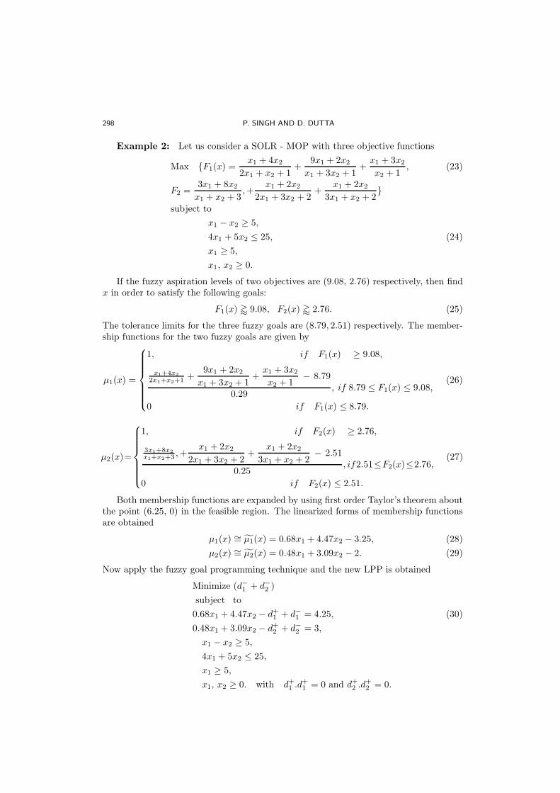
298 P. SINGH AND D. DUTTA
Example 2: Let us consider a SOLR - MOP with three objective functions
Max F1(x) =x1 + 4x2
2x1 + x2 + 1+
9x1 + 2x2
x1 + 3x2 + 1+
x1 + 3x2
x2 + 1, (23)
F2 =3x1 + 8x2
x1 + x2 + 3,+
x1 + 2x2
2x1 + 3x2 + 2+
x1 + 2x2
3x1 + x2 + 2
subject to
x1 − x2 ≥ 5,
4x1 + 5x2 ≤ 25, (24)
x1 ≥ 5,
x1, x2 ≥ 0.
If the fuzzy aspiration levels of two objectives are (9.08, 2.76) respectively, then findx in order to satisfy the following goals:
F1(x) ' 9.08, F2(x) ' 2.76. (25)
The tolerance limits for the three fuzzy goals are (8.79, 2.51) respectively. The member-ship functions for the two fuzzy goals are given by
µ1(x) =
1, if F1(x) ≥ 9.08,
x1+4x2
2x1+x2+1 +9x1 + 2x2
x1 + 3x2 + 1+
x1 + 3x2
x2 + 1− 8.79
0.29, if 8.79 ≤ F1(x) ≤ 9.08,
0 if F1(x) ≤ 8.79.
(26)
µ2(x)=
1, if F2(x) ≥ 2.76,
3x1+8x2
x1+x2+3 ,+x1 + 2x2
2x1 + 3x2 + 2+
x1 + 2x2
3x1 + x2 + 2− 2.51
0.25, if2.51≤F2(x)≤2.76,
0 if F2(x) ≤ 2.51.
(27)
Both membership functions are expanded by using first order Taylor’s theorem aboutthe point (6.25, 0) in the feasible region. The linearized forms of membership functionsare obtained
µ1(x) ∼= µ1(x) = 0.68x1 + 4.47x2 − 3.25, (28)
µ2(x) ∼= µ2(x) = 0.48x1 + 3.09x2 − 2. (29)
Now apply the fuzzy goal programming technique and the new LPP is obtained
Minimize (d−1 + d−2 )
subject to
0.68x1 + 4.47x2 − d+1 + d−1 = 4.25, (30)
0.48x1 + 3.09x2 − d+2 + d−2 = 3,
x1 − x2 ≥ 5,
4x1 + 5x2 ≤ 25,
x1 ≥ 5,
x1, x2 ≥ 0. with d+1 .d+1 = 0 and d+2 .d
+2 = 0.
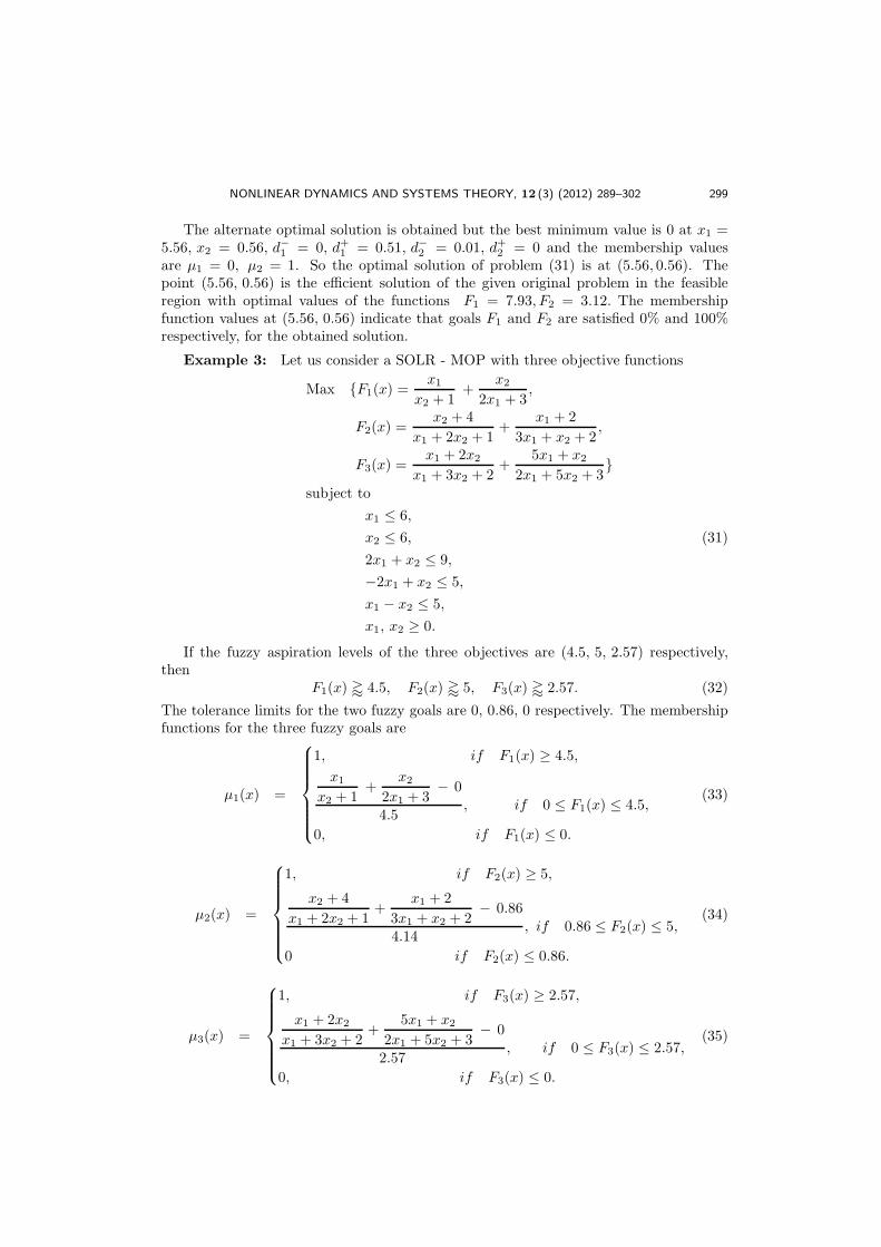
NONLINEAR DYNAMICS AND SYSTEMS THEORY, 12 (3) (2012) 289–302 299
The alternate optimal solution is obtained but the best minimum value is 0 at x1 =5.56, x2 = 0.56, d−1 = 0, d+1 = 0.51, d−2 = 0.01, d+2 = 0 and the membership valuesare µ1 = 0, µ2 = 1. So the optimal solution of problem (31) is at (5.56, 0.56). Thepoint (5.56, 0.56) is the efficient solution of the given original problem in the feasibleregion with optimal values of the functions F1 = 7.93, F2 = 3.12. The membershipfunction values at (5.56, 0.56) indicate that goals F1 and F2 are satisfied 0% and 100%respectively, for the obtained solution.
Example 3: Let us consider a SOLR - MOP with three objective functions
Max F1(x) =x1
x2 + 1+
x2
2x1 + 3,
F2(x) =x2 + 4
x1 + 2x2 + 1+
x1 + 2
3x1 + x2 + 2,
F3(x) =x1 + 2x2
x1 + 3x2 + 2+
5x1 + x2
2x1 + 5x2 + 3
subject to
x1 ≤ 6,
x2 ≤ 6, (31)
2x1 + x2 ≤ 9,
−2x1 + x2 ≤ 5,
x1 − x2 ≤ 5,
x1, x2 ≥ 0.
If the fuzzy aspiration levels of the three objectives are (4.5, 5, 2.57) respectively,then
F1(x) ' 4.5, F2(x) ' 5, F3(x) ' 2.57. (32)
The tolerance limits for the two fuzzy goals are 0, 0.86, 0 respectively. The membershipfunctions for the three fuzzy goals are
µ1(x) =
1, if F1(x) ≥ 4.5,
x1
x2 + 1+
x2
2x1 + 3− 0
4.5, if 0 ≤ F1(x) ≤ 4.5,
0, if F1(x) ≤ 0.
(33)
µ2(x) =
1, if F2(x) ≥ 5,
x2 + 4
x1 + 2x2 + 1+
x1 + 2
3x1 + x2 + 2− 0.86
4.14, if 0.86 ≤ F2(x) ≤ 5,
0 if F2(x) ≤ 0.86.
(34)
µ3(x) =
1, if F3(x) ≥ 2.57,
x1 + 2x2
x1 + 3x2 + 2+
5x1 + x2
2x1 + 5x2 + 3− 0
2.57, if 0 ≤ F3(x) ≤ 2.57,
0, if F3(x) ≤ 0.
(35)
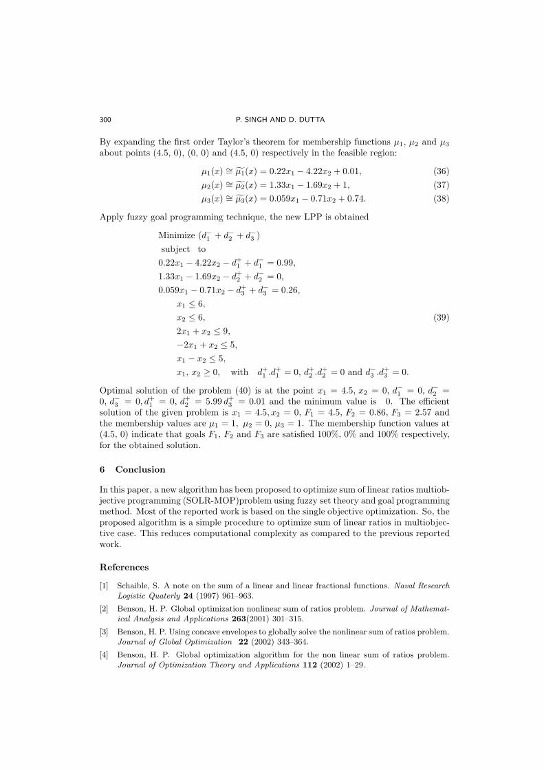
300 P. SINGH AND D. DUTTA
By expanding the first order Taylor’s theorem for membership functions µ1, µ2 and µ3
about points (4.5, 0), (0, 0) and (4.5, 0) respectively in the feasible region:
µ1(x) ∼= µ1(x) = 0.22x1 − 4.22x2 + 0.01, (36)
µ2(x) ∼= µ2(x) = 1.33x1 − 1.69x2 + 1, (37)
µ3(x) ∼= µ3(x) = 0.059x1 − 0.71x2 + 0.74. (38)
Apply fuzzy goal programming technique, the new LPP is obtained
Minimize (d−1 + d−2 + d−3 )
subject to
0.22x1 − 4.22x2 − d+1 + d−1 = 0.99,
1.33x1 − 1.69x2 − d+2 + d−2 = 0,
0.059x1 − 0.71x2 − d+3 + d−3 = 0.26,
x1 ≤ 6,
x2 ≤ 6, (39)
2x1 + x2 ≤ 9,
−2x1 + x2 ≤ 5,
x1 − x2 ≤ 5,
x1, x2 ≥ 0, with d+1 .d+1 = 0, d+2 .d
+2 = 0 and d−3 .d
+3 = 0.
Optimal solution of the problem (40) is at the point x1 = 4.5, x2 = 0, d−1 = 0, d−2 =0, d−3 = 0, d+1 = 0, d+2 = 5.99 d+3 = 0.01 and the minimum value is 0. The efficientsolution of the given problem is x1 = 4.5, x2 = 0, F1 = 4.5, F2 = 0.86, F3 = 2.57 andthe membership values are µ1 = 1, µ2 = 0, µ3 = 1. The membership function values at(4.5, 0) indicate that goals F1, F2 and F3 are satisfied 100%, 0% and 100% respectively,for the obtained solution.
6 Conclusion
In this paper, a new algorithm has been proposed to optimize sum of linear ratios multiob-jective programming (SOLR-MOP)problem using fuzzy set theory and goal programmingmethod. Most of the reported work is based on the single objective optimization. So, theproposed algorithm is a simple procedure to optimize sum of linear ratios in multiobjec-tive case. This reduces computational complexity as compared to the previous reportedwork.
References
[1] Schaible, S. A note on the sum of a linear and linear fractional functions. Naval ResearchLogistic Quaterly 24 (1997) 961–963.
[2] Benson, H. P. Global optimization nonlinear sum of ratios problem. Journal of Mathemat-ical Analysis and Applications 263(2001) 301–315.
[3] Benson, H. P. Using concave envelopes to globally solve the nonlinear sum of ratios problem.Journal of Global Optimization 22 (2002) 343–364.
[4] Benson, H. P. Global optimization algorithm for the non linear sum of ratios problem.Journal of Optimization Theory and Applications 112 (2002) 1–29.
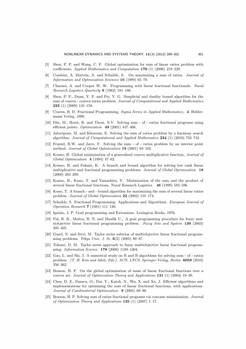
NONLINEAR DYNAMICS AND SYSTEMS THEORY, 12 (3) (2012) 289–302 301
[5] Shen, P. P. and Wang, C. F. Global optimization for sum of linear ratios problem withcoefficients, Applied Mathematics and Computation 176 (1) (2006) 219–229.
[6] Combini, A. Martein, A. and Schaible, S. On maximizing a sum of ratios. Journal ofInformation and Optimization Sciences 10 (1989) 65–79.
[7] Charnes, A. and Cooper W. W. Programming with linear fractional functionals. NavalResearch Logistics Quarterly 9 (1962) 181–186.
[8] Shen, P. P., Duan, Y. P. and Pei, Y. G. Simplicial and duality bound algorithm for thesum of convex - convex ratios problem. Journal of Computational and Applied Mathematics223 (1) (2009) 145–158.
[9] Craven, B. D. Fractional Programming, Sigma Series in Applied Mathematics, 4. Helder-mann Verlag, 1998.
[10] Dur, M., Horst, R. and Thoai, N.V. Solving sum - of - ratios fractional programs usingefficient points. Optimization 49 (2001) 447–466.
[11] Jaberipour, M. and Khorram, E. Solving the sum of ratios problem by a harmony searchalgorithm. Journal of Computational and Applied Mathematics 234 (1) (2010) 733–742.
[12] Fruend, R.W. and Jarre, F. Solving the sum - of - ratios problem by an interior pointmethod. Journal of Global Optimization 19 (2001) 83–102.
[13] Konno, H. Global minimization of a generalized convex multiplicative function, Journal ofGlobal Optimization 4 (1994) 47–62.
[14] Konno, H. and Fukaisi, K. A branch and bound algorithm for solving low rank linearmultiplicative and fractional programming problems. Journal of Global Oprimization 18(2000) 283–299.
[15] Konno, H., Kuno, T. and Yamashita, Y. Minimization of the sum and the product ofseveral linear fractional functions. Naval Research Logistics 46 (1999) 583–596.
[16] Kuno, T. A branch - and - bound algorithm for maximizing the sum of several linear ratiosproblem .Journal of Global Optimization 22 (2002) 155–174.
[17] Schaible, S. Fractional Programming: Applications and Algorithms. European Journal ofOperation Research 7 (1981) 111–120.
[18] Ignizio, J. P. Goal programming and Extensions. Lexington Books, 1976.
[19] Pal, B. B., Moitra, B. N. and Maulik U., A goal programming procedure for fuzzy mul-tiobjective linear fractional programming problem. Fuzzy Sets and System 139 (2003)395–405.
[20] Guzel, N. and Sivri, M. Taylor series solution of multiobjective linear fractional program-ming problems. Trkya Univ. J. Sc. 6(2) (2005) 80–87.
[21] Toksari, D. M. Taylor series approach to fuzzy multiobjective linear fractional program-ming. Information Science 178 (2008) 1189–1204.
[22] Gao, L. and Shi, J. A numerical study on B and B algorithms for solving sum - of - ratiosproblem . (T. H. Kim and Adeli, Eds.). ACN, LNCS, Springer-Verlag, Berlin 6059 (2010)356–362.
[23] Benson, H. P. On the global optimization of sums of linear fractional functions over aconvex set. Journal of Optimization Theory and Applications 121 (1) (2004) 19–39.
[24] Chen, D. Z., Daescu, O., Dai, Y., Katoh, N., Wu, X. and Xu, J. Efficient algorithms andimplementations for optimizing the sum of linear fractional functions, with applications.Journal of Combinatorial Optimization 9 (2005) 69–90.
[25] Benson, H. P. Solving sum of ratios fractional programs via concane minimization. Journalof Optimization Theory and Applications 135 (1) (2007) 1–17.
302 P. SINGH AND D. DUTTA
[26] Gao, L., Mishra, S. K. and Shi, J. An extension of branch- and - bound algorithm forsolving sum -of- nonlinear-ratios problem. Optimization Letters. Article in press (2010),DOI 10.1007/11590-010-0232-8.
[27] Dutta, D., Tiwari, R. N. and Rao, J. R. Multiple objective linear fractional programming.A fuzzy set theoretic approach. Fuzzy Sets and Systems 52 (1992) 39–45.
[28] Luhandjula, M. K. Fuzzy approches for multiple objective linear fractional optimization.Fuzzy Sets and Systems 13 (1984) 11–23.
[29] Zimmermann, H.J. Fuzzy programming and linear programming with several objectivefunctions. Fuzzy Sets and Systems 1 (1978) 45–55.
[30] Woon, S.F. et. al. Global Optimization method for continuous - time series sensor, Non-linear Dynamics and Systems Theory 10 (2) (2010) 175–188.
[31] Solorzano, C.R.H. et. al. Optimization of transfer of neptune. Nonlinear Dynamics andSystems Theory 8 (2) (2008) 205–211.
[32] Psillakis H. E. et. al. A simple non - linear adaptive - Fuzzy Passive - based control ofpower system. Nonlinear Dynamics and Systems Theory 7 (1) (2007) 51–67.
Nonlinear Dynamics and Systems Theory, 12 (3) (2012) 303–310
Approximate Controllability of Nonlocal Semilinear
Time-varying Delay Control Systems
N.K. Tomar ∗ and S. Kumar
Department of Mathematics, Indian Institute of Technology, Patna 800013, India.
Received: August 25, 2011; Revised: July 1, 2012
Abstract: In this work the controllability problem for a class of semilinear controlsystem with nonlocal initial conditions is considered. Under some simple conditionsthe relation between the reachable set of semilinear system and that of its corre-sponding linear system is established. In particular, approximate controllability ofsemilinear abstract control system is proved. Examples are presented to explain theapplication of the proposed result.
Keywords: infinite-dimensional spaces; semilinear time-varying delay systems; ap-
proximate controllability; nonlocal conditions.
Mathematics Subject Classification (2010): 93B05.
1 Introduction
Let (X, ‖ · ‖) be a Banach space and Ct = C([−τ, t]; X), τ > 0, 0 ≤ t ≤ T < ∞, bea Banach space of all continuous functions from [−τ, t] into X endowed with the norm||φ||Ct
= sup−τ≤η≤t
||φ(η)||. Now, consider the following nonlocal semilinear delay control
system
x′(t) = Ax(t) +Bu(t) + f(t, x(t), xb(t)) on (0, T ],
h(x) = φ on [−τ, 0], (1)
where the state variable x(·) takes values in Banach space X and the control functionu(·) belongs to Y = L2([0, T ];U), the Banach space of admissible control functions witha Banach space U . Standing assumptions on system operators are as follows:
∗ Corresponding author: mailto:[email protected]
c© 2012 InforMath Publishing Group/1562-8353 (print)/1813-7385 (online)/http://e-ndst.kiev.ua303
304 N.K. TOMAR AND S.KUMAR
(H1) A : X ⊃ D(A) → X is a linear operator such that it generates a C0-semigroup onX ,denoted by S(t) : t ≥ 0. Let M ≥ 1 and ω ≥ 0 be such that ||S(t)|| ≤ Meωt; t ≥ 0.
(H2) b : [0, T ] → [0, T ] is a map such that it satisfies the property b(t) ≤ t, ∀t ∈ [0, T ].For a continuous function x ∈ CT and t ∈ [0, T ], xb(t) ∈ C0 and is defined byxb(t)(θ) = x(b(t) + θ); θ ∈ [−τ, 0].
(H3) h : C0 → C0, and there exists a function χ ∈ C0 such that h(χ) = φ.
(H4) Nonlinear map f : [0, T ]×X × C0 → X is continuous in first variable and satisfiesthe Lipschitz-like condition in second and third argument, that is, there exists someconstant l > 0 such that ‖f(t, x(t), yb(t))− f(t, v(t), wb(t))‖ ≤ l(‖x− v‖CT
+ ‖y −w‖CT
) for all x, y, v, w ∈ CT and t ∈ [0, T ].
(H5) B : U → X is a bounded linear operator.
Semilinear differential equation (1) can be seen as an abstract formulation for manycontrol systems described by partial or functional differential equations. Here, nonlocalcondition is generally more practical for the physical measurements as compared to theclassical condition. The importance of nonlocal conditions has been discussed in the pio-neering work by Byszewski and Lakshmikantham [6,7]. Nonlocal conditions were used byDeng in [10] to describe, for instance, the diffusion phenomenon of a small amount of gasin a transparent tube. It is a well known fact that the problem of controllability of semi-linear systems in infinite-dimensional spaces can be converted into solvability problem ofa functional operator equation in appropriate Banach spaces, and fixed-point theory hasbeen widely used in the literature to establish this solvability; [2,9,14,15]. These conceptshas been extended to infinite-dimensional semilinear delay control systems with local ornonlocal initial conditions, among others, we refer to the papers [5, 17, 19, 21, 23, 24, 26]for local conditions and papers [3, 4, 13, 16] for nonlocal conditions.
The purpose of this paper is to compare the trajectory reachable set of nonlinearsystem (1) to the trajectory reachable set of its corresponding linear system [f = 0in (1)] and this is motivated by the paper of Naito and Park [19] and Ryu, Park, andKwun [21]. In particular, approximate controllability of system (1) is shown provided thecorresponding linear system is controllable. In the proof of the main controllability resultin the next section, we do not require any inequality condition, compactness of S(t), anduniform-boundedness of f . In this respect, this paper relaxes some restrictions made byearlier authors if an another simple condition is satisfied by the system operators. In thelast section, theory is illustrated with some examples.
2 The Main Results
Let us first consider the following functional delay differential system:
x′(t) = Ax(t) + f(t, x(t), xb(t)), t ∈ (0, T ],h(x) = φ, on [−τ, 0].
(2)
Definition 2.1 A solution function x ∈ CT of the integral equation
x(t) = χ(t), t ∈ [−τ, 0],
S(t)χ(0) +∫ t
0 S(t− s)f(s, x(s), xb(s))ds, t ∈ [0, T ],(3)
is called a mild solution of problem (2).
NONLINEAR DYNAMICS AND SYSTEMS THEORY, 12 (3) (2012) 303–310 305
The existence and uniqueness of the mild solution of (2) is discussed in the followingtheorem, and the proof is motivated by the work of Bahuguna and his coworkers, see[1, 11].
Theorem 2.1 If assumptions (H1)-(H4) are satisfied, then there exists a mild solu-tion of (2) on [0, T ] for some T > 0. Moreover, the mild solution is unique if and onlyif χ is unique.
Proof. We choose a T > 0 such that 2lTMeωT < 1. Define a map F from CT intoitself by
(Fx)(t) = χ(t), t ∈ [−τ, 0],
S(t)χ(0) +∫ t
0S(t− s)f(s, x(s), xb(s))ds, t ∈ [0, T ].
(4)
It is clear that F is well defined and assumption (H3) ensures a fixed point of F ont ∈ [−τ, 0]. Now we show that F is a contraction for the case when t ∈ [0, T ]. For thispurpose, consider any x, y ∈ CT , then we have
||(Fx)(t) − (Fy)(t)||X ≤ ||∫ t
0
S(t− s)(f(s, x(s), xb(s))− f(s, y(s), yb(s)))ds||X
≤ 2lTMeωT ||x− y||CT. (5)
Since 2lTMeωT < 1, F is a contraction on CT and hence by Banach Contraction PrincipleF has a unique fixed point. Obviously, the uniqueness of χ in (H3) reveals the uniquenessof the mild solution. 2
From the above result, a mild solution of the control system (1) can be written asfollows
x(t) = χ(t), t ∈ [−τ, 0],
S(t)χ(0) +∫ t
0S(t− s)[Bu(s) + f(s, x(s), xb(s))]ds, t ∈ [0, T ].
(6)
Note that, mild solution (6) depends on control functions u(·). The solution of (6)under a control u(·), denoted by x(·;u), is called the trajectory (state) function of (1)under u(·). The set of all possible trajectories, denoted by
Kα(f) := x(·;u) ∈ C([α, T ]; X) : u ∈ L2([0, T ];U), 0 < α ≤ T (7)
is called the trajectory reachable set of system (1). In particular, the set of all possibleterminal states, denoted by
KT (f) := x(T ;u) ∈ X : u ∈ L2([0, T ];U) (8)
is called the reachable set of system (1) at terminal time T .
Definition 2.2 System (1) is said to be approximate controllable on [0, T ] ifKT (f) = X , where KT (f) stands for the closure of KT (f) in X .
Now, we define two functions F : CT → L2([0, T ];X) and B1 : Y → L2([0, T ];X ] as(Fx)(t) = f(t, x(t), xb(t)), (B1u)(t) = Bu(t).
Theorem 2.2 Under assumptions (H1)-(H5) and R(F ) ⊆ R(B1), we have Kα(f) ⊇Kα(0).
306 N.K. TOMAR AND S.KUMAR
Proof. Let x(·) ∈ Kα(0), there exists a control u ∈ Y such that
x(t) = χ(t), t ∈ [−τ, 0],
S(t)χ(0) +∫ t
0S(t− s)Bu(s)ds, t ∈ [0, T ].
(9)
Due to range condition, for a given ǫ > 0 ∃ w ∈ Y such that
‖Fx−B1w‖L2([0,T ];X) ≤ ǫ. (10)
Now, let y(·) be mild solution of (1) corresponding to control u− w. Then
x(t) − y(t) =
∫ t
0
S(t− s)Bw(s)ds−∫ t
0
S(t− s)f(s, y(s), yb(t))ds
=
∫ t
0
S(t− s)(B1w − Fx)(s)ds+
∫ t
0
S(t− s)(Fx− Fy)(s)ds. (11)
Using (H4) and (10) we have
‖x(t)− y(t)‖ ≤ MeωT
∫ t
0
‖(B1w − Fx)(s)‖ds+MeωT
∫ t
0
‖(Fx− Fy)(s)‖ds
≤ MeωT√Tǫ+ 2MleωT
∫ t
0
||x− y||CTds.
(12)
This implies
||x− y||CT≤ MeωT
√Tǫ+ 2MleωT
∫ t
0
||x− y||CTds. (13)
Now, using Gronwall’s inequality it can be shown that
||x− y||CT≤ MeωT
√Tǫ exp(2lTMeωT ). (14)
From the above inequality it is clear that ||x − y||CTcan be made arbitrary small by
choosing suitable w. Hence the theorem is proved. 2
Corollary 2.1 Under assumptions of the above theorem, system (1) is approximatecontrollable if its corresponding linear system is approximate or exact controllable.
Proof. The proof is a particular case of Theorem 2.2 at α = T . 2
Remark 2.1 Fixed-point theory arguments make it necessary to assume uniformboundedness of nonlinear term f with certain inequality condition involving various sys-tem parameters, and/or compactness of semigroup T (t). But, these conditions (speciallyinequality conditions) are not easy to verify in many situations. In this paper theseconditions are replaced with a range condition R(F ) ⊂ R(B1). Note that this rangecondition is satisfied trivially for the system (1) if B is the identity operator. Obviously,Theorem 2.2 gives the controllability of system (1) when b(t) = t in the case of constantdelay, and this case is explained in Example 3.1.
NONLINEAR DYNAMICS AND SYSTEMS THEORY, 12 (3) (2012) 303–310 307
3 Application
Example 3.1 Consider the following mathematical model
∂
∂ty(t, x) =
∂2
∂x2y(t, x) + u(t, x) + (
∫ 1
0
y(t, x)dx)y(t, x)
+ (
∫ 1
0
y(t− τ, x)dx)y(t − τ, x), 0 ≤ x ≤ 1, t ∈ [0, T ], (15)
y(t, 0) = y(t, 1) = 0, t ∈ [0, T ],
1
τ
∫ 0
−τ
e2sy(s, x)ds = y0(x), 0 ≤ x ≤ 1,
where y(t, .), u(t, .), y0 ∈ L2(0, 1). If we take
(1) X = L2(0, 1) as the state space and y(t, ·) = y(t, x) : 0 ≤ x ≤ 1 as the state.
(2) input trajectory u(t, .) as the control and U = L2(0, 1) as the control space. Notethat, here X = U .
(3) A : D(A) ⊂ X → X defined by A(z) = d2zdx2 with domain D(A) =
H2(0, 1)⋂
H10 (0, 1). Then A is an infinitesimal generator of a C0-semigroup of
bounded linear operators; see [8].
(4) B = I.
(5) b(t) = t, and yb(t)(θ) ≡ y(t− τ, ·) (so this is a constant time-delay case).
(6) f : [0, T ]×X × C0 → X , T > 0 defined by
f(t, y(t, ·), yb(t)) = (
∫ 1
0
y(t, x)dx)y(t, ·) + (
∫ 1
0
y(t− τ, x)dx)y(t − τ, ·),
where 0 ≤ x ≤ 1, t ∈ [0, T ]. It is not hard to see that f satisfies (H4).
(7) h(z)(θ) = g(z) for z ∈ C0, θ ∈ [−τ, 0]; φ(θ) = y0. Here, g : C0 → X is such that
g(z)(x) = 1τ
∫ 0
−τe2sz(s, x)ds. For this definition of h, we can find a function χ ∈ C0,
given by χ(θ) = 1ky0 on [−τ, 0] with k =
∫ τ
01τe−2sds 6= 0, such that
h(χ)(θ) =1
τ
∫ 0
−τ
e2s(1
ky0)ds = y0 = φ(θ), that is, h(χ) = φ.
Then (15) resembles control system (1) and has a mild solution (6) on [−τ, T ]. Now takeY := L2([0, T ];L2(0, 1)), B1 = I : Y → Y , F : CT → Y as (Fz)(t) = f(t, z(t), zb(t)).
Then it is clear that R(F ) ⊂ R(B1). Since the corresponding linear system is approx-imate controllable; [8], system (15) is approximate controllable due to Theorem 2.2.Mathematical model (15) may be seen as the population dynamics, see [12], where
y(t, .) represents the population density at time t and the term ∂2
∂x2 y(t, x) describes theinternal migration. Moreover, the continuous functions B,D : [0, T ] → R+ given by
B(t) =∫ 1
0 y(t− τ, x)dx and D(t) =∫ 1
0 y(t, x)dx, represent average birth and death rates,respectively, τ is the delay due to pregnancy, and source term u(t, x) represents a control.
308 N.K. TOMAR AND S.KUMAR
Example 3.2 Consider the control system governed by the following semilinear heatequation
∂y(t, x)
∂t=
∂2y(t, x)
∂x2+Bu(t, x)
+ f(t, y, yb(t)); 0 < t < T, 0 < x < π, −τ ≤ θ ≤ 0,
y(t, 0) = y(t, π) = 0, t ∈ [0, T ], (16)
with the same initial condition as in the above example, where y(t, .), y0 ∈ L2(0, π).Then (16) can be converted into (1), if we take:
(1) X = L2(0, π) as the state space and y(t, .) = y(t, x) : 0 ≤ x ≤ π as the state.
(2) input trajectory u(t, .) as the control.
(3) A : D(A) ⊂ X → X defined by A(z) = d2zdx2 with domain D(A) =
H2(0, π)⋂
H10 (0, π). Then, D(A) = X and A is an infinitesimal generator of a
C0-semigroup of bounded linear operators; see [8]. Further, if we take φn(x) =(2/π)1/2 sin(nx); 0 6 x 6 π;n ∈ N, then φn is an orthonormal basis of X andφn is an eigenfunction corresponding to the eigenvalue λn = −n2 of operator A.Then the C0-semigroup generated by A has eλnt as the eigenvalues and φn as theircorresponding eigenfunctions.
(4) U = u : u =∑∞
n=2 unφn :∑∞
n=2 u2n < ∞, with norm |u|U = (
∑∞n=2 u
2n)
1/2 as thecontrol space. B is a continuous linear map from U to X defined as
Bu = 2u2φ1 +
∞∑
n=2
unφn for u =
∞∑
n=2
unφn ∈ U.
(5) b(t) = k| sin t|, k ∈ (0, 1) or b(t) = t2
1+t2.
(6) h and χ are the same as in Example 3.1.
It shows that (16) has a mild solution (6) on [−τ, T ] provided f is Lipschitz con-tinuous. Although, the same example has been discussed in [9, 18, 27] (with or with-out delay and under local conditions), but approximate controllability was proved un-der restrictions such as the uniform boundedness on f or some inequality constraints.This paper shows that the approximate controllability also follows for non-uniformbounded function f without having to satisfy any inequality constraint and withoutusing the compactness of C0-semigroup. For example, consider the function f given byf(t, z, zb(t)) = α(‖z‖CT
+ ‖zb(t)‖C0)(φ3(x) + φ4(x)), where α is a positive constant. Here
f is Lipschitz and R(F ) ⊆ R(B1). Moreover, this example shows that time-varying affer-effect and generalized nonlocal conditions can also be handled by the theorem proved in
the previous section. In the above example b(t) = k| sin t|, k ∈ (0, 1) or b(t) = t2
1+t2is a
theoretical construction but many physical and biological processes include time-varyingaffereffect phenomena in their inner dynamics, see [20].
Example 3.3 Consider the system of infinite ordinary differential equations:
dx(t)
dt= Ax(t) + u(t) + f(t, x(t), xb(t)),
l∑
i=1
cix(θi) = x0, (17)
where x(t) = (x1(t), x2(t), . . .) ∈ l2. Then (17) resembles control system (1), if we take
NONLINEAR DYNAMICS AND SYSTEMS THEORY, 12 (3) (2012) 303–310 309
(1) X = l2 as the state space and x(t) as the state.
(2) input u(t) = (u1(t), u2(t), . . .) as the control and U = l2 as the control space. Notethat, here X = U .
(3) A is a self-adjoint operator onX defined by Aei = λiei where ei is an orthonormalbasis of X and λiis a decreasing sequence of positive numbers such that lim
i→∞λi =
λ0 > 0. Then A is an infinitesimal generator of a C0-semigroup of bounded linear
operators defined by T (t)x =
(
eλ1tx1, eλ2tx2, . . .
)
.
(4) B = I and b is the same as in Example 3.2.
(5) f is defined by f(t, x(t), xb(t)) = (f1(t, x(t), xb(t)), f2(t, x(t), xb(t)), . . .), 0 ≤ t ≤ T .
(6) h(z)(θ) = g(z) for z ∈ C0, θ ∈ [−τ, 0]; φ(θ) = x0. Here, g : C0 → X is such that
g(z) =∑l
i=1 ciz(θi);−τ ≤ θ1 < θ2 < · · · < θl ≤ 0. For this definition of h, we can
find a function χ ∈ C0, given by χ(θ) = 1kx0 on [−τ, 0] with k =
∑l
i=1 ci.
The approximate controllability of the linear system corresponding to (17) has beenproved by Triggiani [25]. In [22], the approximate controllability of (17) (without delayand with local Cauchy condition) has been shown via the solvability of some operatorequations under the following conditions:
(i) The linear system is approximate controllable,(ii) A generates a compact semigroup T (t),(iii) The nonlinear operator f(t, x) satisfies the Lipschitz condition,(iv) The operator f satisfies the growth condition ‖f(x(t))‖X ≤ a‖x(t)‖X + b,
(v) System constants satisfy the constraint eλ1T√T
2 ·√
2MbT (e2MbT − 1) <e2Tλ0−1
2eλ1T√Tλ0
, where ‖T (t)‖ ≤ eλ1τ = M for 0 ≤ t ≤ T .
But due to Theorem 2.2, it follows that the system (17) is approximate controllableonly under the above conditions (i) and (iii) for nonlinear operators those satisfy therange condition, e.g. f is defined as f1(t, x(t), xb(t)) = a‖x‖ + b‖xb(t)‖ + c; a, b, andc are positive constants and fi(t, x(t), xb(t)) = 0 for all i = 2, 3, . . .. This shows thatthe inequalities such as (v) above, assumed by earlier author are not required to beconsidered.
References
[1] Bahuguna, D., Shukla, R.K. and Saxena, S. Functional Differential Equations with NonlocalConditions in Banach Spaces. Nonlinear Dynamics and Systems Theory 10(4) (2010) 317–323.
[2] Balachandran, K. and Dauer, J.P. Controllability of Nonlinear Systems in Banach Spaces:A Survey. J. Optimization Theory and Applications 115(1) (2002) 7–28.
[3] Balachandran, K., Park, J.Y. and Park, S.H. Controllability of nonlocal impulsive quasi-linear integrodifferential systems in Banach spaces. Reports on Mathematical Physics 65(2)(2010) 247–257.
[4] Benchohra, M., Gatsor, E. P., Gorniewicz, L. and Ntouyas, S.K. Controllability Results forEvolution Inclusions with Non-Local Conditions. Journal for Analysis and its Applications
22(2) (2003) 411–431.
310 N.K. TOMAR AND S.KUMAR
[5] Bouzahir, H. and Fu, X.-L. Controllability of neutral functional differential equations withinfinite delay. Acta mathematica scientia 31(1) (2011) 73–80.
[6] Byszewski, L. Theorems about the existence and uniqueness of solutions of a semilinearevolution nonlocal Cauchy problem, J. Math. Anal. Appl. 162 (1991) 494–505.
[7] Byszewski, L. and Lakshmikantham, V. Theorems about the existence and uniqueness ofsolutions of a nonlocal abstract Cauchy problem in a Banach space. Appl. Anal. 40 (1990)11–19.
[8] Curtain, R.F. and Zwart, H.J. An Introduction to infinite-dimensional linear systems the-
ory. Springer-Verlag, New York, 1995.
[9] Dauer, J. P. and Mahmudov, N. I. Approximate Controllability of Semilinear FunctionalEquations in Hilbert Spaces. J. Math. Anal. Appl. 273 (2002) 310–327.
[10] Deng, K. Exponential decay of solutions of semilinear parabolic equations with nonlocalinitial conditions. Journal of Mathematical analysis and applications. 179 (1993) 630–637.
[11] Dubey, S.A. and Bahuguna, D. Existence and regularity of solutions to nonlocal retardeddifferential equations.Applied Mathematics and Computation 215 (2009) 2413–2424.
[12] Engel, K.J. and Nagel, R. One Parameter Semigroups for Linear Evolution Equations.
Springer-Verlag, Berlin, 1995.
[13] Guo, M., Xue, X. and Li, R. Controllability of Impulsive Evolution Inclusions with NonlocalConditions. J. Optimization Theory and Application 120(2) (2004) 355–374.
[14] Jeong, J.-M. and Kim, H.-G. Controllability of Semilinear Functional IntegrodifferentialEquaions. Bull. Korean Math. Soc. 46(3) (2009) 463–475.
[15] Joshi, M.C. and Sukavanam, N. Approximate solvability of semilinear operator equations.Nonlinearity 3 (1990) 519–525.
[16] Li, G. and Xue, X. Controllability of evolution inclusions with nonlocal conditions. Applied
Mathematics and Computation 141 (2003) 375–384.
[17] Liu, B. Controllability of impulsive neutral functional differential inclusions with infinitedelay. Nonlinear Analysis 60 (2005) 1533–1552.
[18] Naito, K. Controllability of Semilinear Control Systems Dominated by the Linear Part.SIAM Journal on Control and Optimization 25 (1987) 715–722.
[19] Naito, K. and Park, J.Y. Approximate Controllability for trajectories of a delay volterracontrol syatem. J. Optimization Theory and Application 61(2) (1989) 271–279.
[20] Richard, J.-P. Time-delay systems: an overview of some recent advances and open problems.Automatica 39 (2003) 1667–1694.
[21] Ryu, J.W., Park, J.Y. and Kwun, Y.C. Approximate Controllability of delay volterra con-trol syatem. Bull. Korean Math. Soc. 30(2) (1992) 277–284.
[22] Sukavanam, N. Solvability of semilinear operator equations with growing nonlinearity. J.Math. Anal. Appl. 241 (2000) 39–45.
[23] Sukavanam, N. and Tomar, N.K. Approximate controllability of semilinear delay controlsystem. Nonlinear Func. Anal. Appl. 12 (2007) 53–59.
[24] Tomar, N.K and Sukavanam, N. Approximate controllability of non-densely defined semi-linear delayed control systems. Nonlinear Studies 18(2) (2011) 229–234.
[25] Triggiani, R. On the Stabilizability Problem in Banach Space. Journal of Mathematical
Analysis and Applications 52 (1975) 383–403.
[26] Wang, L. Approximate Controllability for semilinear differential equations with unboundeddelay. In: Control and Decision Conference CCDC 2008, Chinese.
[27] Wang, L. Approximate Controllability of Delayed Semilinear Control Systems. J. Applied
Math. and Stochastic Analysis 2005(1) (2005) 67–76.
Nonlinear Dynamics and Systems Theory, 12 (3) (2012) 311–323
Existence of Positive Solutions of a Nonlinear
Third-Order M -Point Boundary Value Problem for
p-Laplacian Dynamic Equations on Time Scales
N. Yolcu ∗ and S. Topal
Department of Mathematics, Ege University,
35100 Bornova, Izmir-Turkey
Received: May 6, 2011; Revised: July 10, 2012
Abstract: In this paper, by using fixed-point theorems in cones, we study theexistence of at least one, two and three positive solution of a nonlinear third-orderm-point p-Laplacian boundary value problem on time scale.
Keywords: time scales; nontrivial solution; fixed-point theorems.
Mathematics Subject Classification (2010): 39A10, 34B15, 34B16.
1 Introduction
We study the third-order m-point boundary value problems (MPBVP) on time scaleswith p-Laplacian,
(Φp(u∇))∇(t) + p(t)f(t, u(t)) = 0, t ∈ [0, T ]Tk∩Tk2 , (1)
u∇(ρ(0)) = 0, u(T ) = 0, u(ρ(0)) = B(
m−2∑
1
αiu(ξi)), (2)
where Φp is p-Laplacian operator, i.e. Φp(s) = |s|p−2s, p > 1 and (Φp)−1 = Φq with
1p+ 1
q= 1. Here ρ(0) < ξ1 < ξ2 < ... < ξm−2 < σ(T ).
(H1) αi ∈ [0,∞), i = 1, 2, 3... and f : [0, T ]× [0,∞) → [0,∞) is left-dense continuousfunction,
∗ Corresponding author: mailto:[email protected]
c© 2012 InforMath Publishing Group/1562-8353 (print)/1813-7385 (online)/http://e-ndst.kiev.ua311
312 NERMIN YOLCU AND SERAP TOPAL
(H2) p : [0, T ] → [0,∞) is left-dense continuous function,
(H3) B : R → R is continuous and satisfies the existence of B0 ≥ B1 > 0 such thatB0s ≤ B(s) ≤ B1s, for s ∈ [0,∞).
A time scale T is a nonempty closed subset of R. We make the blanket assumption0, T are points in T. By an interval [0, T ], we always mean the intersection of the realinterval [0, T ] with the given time scale; that is [0, T ] ∩T. For t < supT and r > inf T,define the forward jump operator σ and the backward jump operator ρ, respectively,σ(t) = infτ ∈ T|τ > t ∈ T, ρ(r) = supτ ∈ T|τ < r for all t, r ∈ T. If σ(t) > t, t issaid to be right scattered, and if ρ(r) < r, r is said to be left scattered. If σ(t) = t, t issaid to be right dense, and if ρ(r) = r, r is said to be left dense. If T has a right scat-tered minimum m, define Tk = T−m; otherwise set Tk = T. If T has a left scatteredmaximum M , define Tk = T−M; otherwise set Tk = T. Some basic definitions andtheorems on time scales can be found in the books [4, 5].
p-Laplacian problems with two point, three point and multi point boundary condi-tions for ordinary differential equations and difference equations have been studied byseveral authors (see [6, 10, 16] and the references therein). Recently, there has been muchattention paid to the existence of positive solution for second-order and third-order non-linear boundary value problems on time scales [1, 2, 9, 11, 12, 15, 17, 18]. However, to thebest of our knowledge, there are not many results concerning third-order p-Laplaciandynamic equations on time scales.
In [8], Yanging Guo, Changlang Yu, Jufang Wang considered the existence of threepositive solutions for the following m-point boundary value problems on infinite intervals
(ϕp(x′(t)))′ + φ(t)f(t, x(t), x′(t)) = 0, 0 < t <∞, (3)
x(0) =
m−2∑
1
aix′(ηi), lim
t→∞x′(t) = 0. (4)
They used Avery–Henderson fixed-point theorem on a cone to prove the existence ofthree positive solutions to the (3)− (4) nonlinear problems.
In [15], Sihua Liang, Jihui Zhang, Zhiyong Wang prove the existence of three positivesolutions for the following second order m-point boundary value problems
(Φ(p(t)u(t)))∇ + a(t)f(u(t)) = 0, t ∈ [0, T ]Tk∩Tk, (5)
u(0)−B0
(
m−2∑
1
aiu(ξi)
)
= 0, u(T ) = 0. (6)
for some dynamic equations on time scales using Legget–Williams fixed-point theorem.In [11], Zhimin He obtained the existence of at least double positive solutions of the
following three-point boundary value problems
(Φp(u∇))∇ + a(t)f(u(t)) = 0, t ∈ [0, T ], (7)
u(0)−B0(u(η)) = 0, u(T ) = 0, (8)
or
u(0) = 0, u(T ) + B1(u(η) = 0, (9)
NONLINEAR DYNAMICS AND SYSTEMS THEORY, 12 (3) (2012) 311–323 313
by using double fixed-point theorem.In [9], Wei Hang, Maoxing Liu considered the third-order nonlinear problem such
that
(Φp(u∇))∇ + a(t)f(u(t)) = 0, t ∈ [0, T ], (10)
αu(0)− βu(0) = 0, u(T ) =
m−2∑
1
aiu(ξi), u∇(0) = 0. (11)
They used the fixed-point theorem which is given by V.Lakshmikantham in [7] toprove the existence of at least one nontrivial solution to the nonlinear problem (10)−(11).
Motivated by the results [15], in this paper, we will study the existence of multiplepositive solutions of third-order p-Laplacian MPBVP (1)− (2).
The aim of this paper is to establish some simple criteria for the existence of positivesolutions of the p-Laplacian MPBVP (1) − (2). This paper is organized as follows:In Section 2 we first present some properties of the solution of the linear p-LaplacianMPBVP corresponding to (1) − (2). In Section 3, we state the fixed-point theoremsin order to prove main results and we get the existence of at least one, two and threepositive solutions for nonlinear p-Laplacian MPBVP (1)− (2).
2 Preliminaries and Lemmas
To prove main results, we will give several lemmas and the following lemmas arebased on the linear p-Laplacian MPBVP
(Φp(u∇)∇(t) + h(t) = 0, t ∈ [0, T ]Tk∩Tk2 , (12)
u∇(ρ(0)) = 0, u(ρ(0)) = B(
m−2∑
1
aiu(ξi)), u
(T ) = 0. (13)
Lemma 2.1 For h ∈ Cld([0, T ] × R), the problems (12) and (13) have the unique
solution
u(t) = B(
m−2∑
1
ai
∫ T
ξi
Φq(
∫ s
ρ(0)
h(τ)∇τ)∇s) +∫ t
ρ(0)
(
∫ T
r
Φq(
∫ s
ρ(0)
h(τ)∇τ)∇s)r. (14)
Proof. From the equation (12) we can easily obtain
u∇(s) = −Φq(
∫ s
ρ(0)
h(τ)∇τ), u(t) =
∫ T
t
Φq(
∫ s
ρ(0)
h(τ)∇τ)∇s
Therefore, we have
u(t) = u(ρ(0)) +
∫ t
ρ(0)
(
∫ T
r
Φq(
∫ s
ρ(0)
h(τ)∇τ)∇s)r.
Applying the boundary conditions (2.13) we have
u(t) = B(
m−2∑
1
ai
∫ T
ξi
Φq(
∫ s
ρ(0)
h(τ)∇τ)∇s) +∫ t
ρ(0)
(
∫ T
r
Φq(
∫ s
ρ(0)
h(τ)∇τ)∇s)r.
314 NERMIN YOLCU AND SERAP TOPAL
It is easy to see that the p-Laplacian MPBVP (Φp(u∇(t))∇ = 0, u∇(ρ(0)) = 0,
u(ρ(0)) = B(
m−2∑
1
aiu(ξi)) = 0, u(T ) = 0 has only the trival solution. Thus u is the
unique solution of (12) and (13). The proof is complete. 2
Let X denote Banach space Cld([ρ(0), T ], [0,∞)) with the norm ‖u‖ = sup |u(t)|,t ∈ [ρ(0), T ]. Define the cone P ⊂ X by
P = u ∈ X : u(t) > 0, u(t) > 0, t ∈ [ρ(0), T ], u is concave. (15)
For u ∈ P define the operator L by
Lu(t) = B(
m−2∑
1
ai
∫ T
ξi
Φq(
∫ s
ρ(0)
p(τ)f(τ, u(τ))∇τ)∇s)
+
∫ t
ρ(0)
(
∫ T
r
Φq(
∫ s
ρ(0)
p(τ)f(τ, u(τ))∇τ)∇s)r. (16)
Obviously, from the definition of L we have Lu(t) ≥ 0 and for t ∈ [ρ(0), T ] we get
(Lu)(t) =
∫ T
t
Φq(
∫ s
ρ(0)
p(τ)f(τ, u(τ))∇τ)∇s ≥ 0.
As
(Lu)∇(t) = −Φq(
∫ t
ρ(0)
p(τ)f(τ, u(τ))∇τ) ≤ 0,
then Lu is concave. Therefore L : P → P and ‖Lu‖ = sup |Lu(t)| = Lu(T ) fort ∈ [ρ(0), T ].
Also it is easy to check that L is a completely continuous operator by a standardapplication of the Arzela-Ascoli theorem.
Lemma 2.2 If u ∈ P and ‖u‖ = sup |u(t)|, t ∈ [ρ(0), T ], then
u(t) ≥ t− ρ(0)
T − ρ(0)‖u‖. (17)
Proof. It can be easily shown by the similar way as in Lemma 3.1 in the reference[14].
3 Existence of Positive Solutions
In this section we will prove the existence of multiple positive solutions of our problem.We will need also the following Krasnoselkii’s fixed-point theorem to prove the existenceof at least one positive solution of p-Laplacian MPBVP (1)–(2).
Theorem 3.1 [13] Let X be a Banach space and P ⊂ X be a cone. Assume Ω1
and Ω2 are open bounded subsets of P with 0 ∈ P, Ω1 ⊂ Ω2, and let
L : P ∩ (Ω2\Ω1) → P be a completely continuous operator such that either
(i) ‖Lu‖ ≤ ‖u‖ for u ∈ P ∩ ∂Ω1, ‖Lu‖ ≥ ‖u‖ for u ∈ P ∩ ∂Ω2;
or
(ii) ‖Lu‖ ≥ ‖u‖ for u ∈ P ∩ ∂Ω1, ‖Lu‖ ≤ ‖u‖ for P ∩ ∂Ω2 hold.
Then L has a fixed point in P ∩ (Ω2\Ω1).
NONLINEAR DYNAMICS AND SYSTEMS THEORY, 12 (3) (2012) 311–323 315
Theorem 3.2 Assume conditions (H1) − (H3) are satisfied. In addition, suppose
there exist numbers 0 < r < R <∞ such that
(i) f(τ, u(τ)) ≤ Φp(u
k1), if 0 ≤ u ≤ r,
and
(ii) f(τ, u(τ)) ≥ Φp(u
k2), if R ≤ u ≤ ∞,
where
k1 = B1
m−2∑
1
ai
∫ T
ξi
Φq(
∫ s
ρ(0)
p(τ)∇τ)∇s +∫ T
ρ(0
(
∫ T
r
Φq(
∫ s
ρ(0)
p(τ)∇τ)∇s)r,
k2 =
∫ T
ρ(0)
(
∫ T
r
Φq(
∫ s
ρ(0)
p(τ)Φp(τ
T)∇τ)∇s)r.
Then the p-Laplacian MPBVP (1)− (2) has at least one positive solution.
Proof. Define the cone P as in (15). It is also easy to check that L : P → P iscompletely continuous and LP ⊂ P . If u ∈ P with ‖u‖ = r then we get
‖Lu‖ ≤ B(
m−2∑
1
ai
∫ T
ξi
Φq(
∫ s
ρ(0)
p(τ)|f(τ, u(τ))|∇τ)∇s)
+
∫ T
ρ(0)
(
∫ T
r
Φq(
∫ s
ρ(0)
p(τ)|f(τ, u(τ))|∇τ)∇s)r
≤ B1
m−2∑
1
ai
∫ T
ξi
Φq(
∫ s
ρ(0)
p(τ)Φp(u
k1)∇τ)∇s
+
∫ T
ρ(0)
(
∫ T
r
Φq(
∫ s
ρ(0)
p(τ)Φp(u
k1)∇τ)∇s)r
=u
k1[B1
m−2∑
1
ai
∫ T
ξi
Φq(
∫ s
ρ(0)
p(τ)∇τ)∇s
+
∫ T
ρ(0)
(
∫ T
r
Φq(
∫ s
ρ(0)
p(τ)∇τ)∇s)r]
= ‖u‖.
So if we set
Ω1 = u ∈ Cld([ρ(0), T ], [0,∞)) : ‖u‖ < r,
then ‖Lu‖ ≤ ‖u‖ for u ∈ P ∩ ∂Ω1.Let us now set
Ω2 = u ∈ Cld([ρ(0), T ], [0,∞)) : ‖u‖ < R,
316 NERMIN YOLCU AND SERAP TOPAL
then for u ∈ P with ‖u‖ = R, we have
‖Lu‖ = |B(
m−2∑
1
ai
∫ T
ξi
Φq(
∫ s
ρ(0)
p(τ)f(τ, u(τ))∇τ)∇s)
+
∫ T
ρ(0)
(
∫ T
r
Φq(
∫ s
ρ(0)
p(τ)f(τ, u(τ))∇τ)∇s)r|
≥∫ T
ρ(0)
(
∫ T
r
Φq(
∫ s
ρ(0)
p(τ)|f(τ, u(τ))|∇τ)∇s)r
≥∫ T
ρ(0)
(
∫ T
r
Φq(
∫ s
ρ(0)
p(τ)Φp(u
k2)∇τ)∇s)r
≥∫ T
ρ(0)
(
∫ T
r
Φq(
∫ s
ρ(0)
p(τ)Φp(τ
T
‖u‖k2
)∇τ)∇s)r
=‖u‖k2
[
∫ T
ρ(0)
(
∫ T
r
Φq(
∫ s
ρ(0)
p(τ)Φp(τ
T)∇τ)∇s)r
= ‖u‖.
Hence ‖Lu‖ ≥ ‖u‖ for u ∈ P ∩ ∂Ω2. Thus by the first part of Theorem 3.1, L has afixed point u ∈ P ∩ (Ω2\Ω1).
Therefore the p-Laplacian MPBVP (1) − (2) has at least one positive solution. 2
Applying the following Avery–Henderson fixed point theorem, we will prove the ex-istence of at least two positive solutions to the p-Laplacian MPBVP (1)− (2).
Theorem 3.3 [3] Let P be a cone in a real Banach space X. Set
P (ψ, z) = u ∈ P : ψ(u) < zIf η and ψ are increasing, nonnegative continuous functionals on P, let θ be a nonnegative
continuous functional on P with θ(0) = 0 such that, for some positive constants z and γψ(u) ≤ θ(u) ≤ η(u) and ‖u‖ ≤ γψ(u)
for all u ∈ P (ψ, z). Suppose that there exist positive numbers x < y < z such that
θ(λu) ≤ λθ(u) for all 0 < λ < 1 and u ∈ ∂P (θ, y).If L : P (ψ, z) → P is completely continuous operator satisfying
(i) ψ(Lu) > z for all u ∈ ∂P (ψ, z)(ii) θ(Lu) < y for all u ∈ ∂P (θ, y)(iii) P (η, x) 6= ∅ and η(Lu) > x for all u ∈ ∂P (η, x). Then L has at least two fixed
points u1 and u2 such that
x < η(u1) with θ(u1) < y and y < θ(u2) with ψ(u2) < z.
Theorem 3.4 Assume (H1)− (H3) hold. Suppose there exist positive numbers x <FEy < (ξ1−ρ(0))F
(T−ρ(0))E z such that the function f satisfies the following conditions:
(i) f(s, u) > Φp(zD) for s ∈ [ξ1, T ] and u ∈ [z, T−ρ(0)
ξ1−ρ(0)z],
(ii) f(s, u) < Φp(yE) for s ∈ [ρ(0), T ] and u ∈ [0, T−ρ(0)
ξ1−ρ(0)y],
(iii) f(s, u) > Φp(xF) for s ∈ [ρ(0), ξm−2] and u ∈ [0, T−ρ(0)
ξm−2−ρ(0)x].
for some positive constants D, E and F. Then p-Laplacian MPBVP (1)− (2) has at leasttwo positive solutions u1 and u2 such that
u1(ξ1) < y and u1(ξm−2) > x, u2(ξ1) > y and u2(ξ1) < z.
NONLINEAR DYNAMICS AND SYSTEMS THEORY, 12 (3) (2012) 311–323 317
Let us define the positive constants D, E and F such that
D = B0
m−2∑
1
ai
∫ T
ξi
Φq(
∫ ξ1
ρ(0)
p(τ)∇τ)∇s +∫ ξ1
ρ(0)
(
∫ T
ξ1
Φq(
∫ ξ1
ρ(0)
p(τ)∇τ)∇s)r,
E = B1
m−2∑
1
ai
∫ T
ξi
Φq(
∫ T
ρ(0)
p(τ)∇τ)∇s +∫ ξ1
ρ(0)
(
∫ T
ρ(0)
Φq(
∫ T
ρ(0)
p(τ)∇τ)∇s)r,
F = B0
m−2∑
1
ai
∫ T
ξi
Φq(
∫ ξm−2
ρ(0)
p(τ)∇τ)∇s +∫ ξm−2
ρ(0)
(
∫ T
ξm−2
Φq(
∫ ξm−2
ρ(0)
p(τ)∇τ)∇s)r.
Proof. Define the cone P as in (15). We know L is completely continuous andLP ⊂ P . Let the nonnegative increasing continuous functionals ψ, θ and η be defined onthe cone byψ(u) = minu(t) = u(ξ1), t ∈ [ξ1, ξm−2],θ(u) = maxu(t) = u(ξ1), t ∈ [ρ(0), ξ1],η(u) = maxu(t) = u(ξm−2), t ∈ [ρ(0), ξm−2].
For each u ∈ P , ψ(u) = θ(u) ≤ η(u). In addition for each u ∈ P
ψ(u) = u(ξ1) ≥ξ1 − ρ(0)
T − ρ(0)‖u‖. (18)
Also θ(0) = 0 and we have θ(λu) = λθ(u) and for u ∈ P and λ ∈ [0, 1] .We now verify that all conditions of Theorem 3.3 are satisfied.
If u ∈ ∂P (ψ, z) then ψ(u) = mint∈[ξ1,ξm−2]u(t) = u(ξ1) = z. So we have u(t) ≥ z, for
t ∈ [ξ1, T ], and from (18) z ≤ u(t) ≤ ‖u‖ ≤ T−ρ(0)ξ1−ρ(0)z for t ∈ [ξ1, T ]. Then assumption (i)
implies f(s, u) > Φp(zD) for s ∈ [ξ1, T ].
Since Lu ∈ P we get
ψ(Lu) = Lu(ξ1)
= B(m−2∑
1
ai
∫ T
ξi
Φq(
∫ s
ρ(0)
p(τ)f(τ, u(τ))∇τ)∇s)
+
∫ ξ1
ρ(0)
(
∫ T
r
Φq(
∫ s
ρ(0)
p(τ)f(τ, u(τ))∇τ)∇s)r
> B0
m−2∑
1
ai
∫ T
ξi
Φq(
∫ s
ρ(0)
p(τ)f(τ, u(τ))∇τ)∇s
+
∫ ξ1
ρ(0)
(
∫ T
ξ1
Φq(
∫ s
ρ(0)
p(τ)f(τ, u(τ))∇τ)∇s)r
> B0
m−2∑
1
ai
∫ T
ξi
Φq(
∫ ξ1
ρ(0)
p(τ)f(τ, u(τ))∇τ)∇s
+
∫ ξ1
ρ(0)
(
∫ T
ξ1
Φq(
∫ ξ1
ρ(0)
p(τ)f(τ, u(τ))∇τ)∇s)r
318 NERMIN YOLCU AND SERAP TOPAL
>z
DB0
m−2∑
1
ai
∫ T
ξi
Φq(
∫ ξ1
ρ(0)
p(τ)∇τ)∇s
+
∫ ξ1
ρ(0)
(
∫ T
ξ1
Φq(
∫ ξ1
ρ(0)
p(τ)∇τ)∇s)r
= z.
Hence condition (i) of Theorem 3.3 is satisfied.Secondly, we show that (ii) of Theorem 3.3 is fulfilled. For this, we select u ∈ ∂P (θ, y).
Thenθ(u) = max
t∈[ρ(0),ξ1]u(t) = u(ξ1) = y.
We know from (2.17)
0 ≤ u(t) ≤ T − ρ(0)
ξ1 − ρ(0)y,
for t ∈ [ρ(0), T ]. Then assumption (ii) implies
f(s, u) < Φp(y
E),
for s ∈ [ρ(0), T ]. Therefore
θ(Lu) = Lu(ξ1)
= B(
m−2∑
1
ai
∫ T
ξi
Φq(
∫ s
ρ(0)
p(τ)f(τ, u(τ))∇τ)∇s)
+
∫ ξ1
ρ(0)
(
∫ T
r
Φq(
∫ s
ρ(0)
p(τ)f(τ, u(τ))∇τ)∇s)r
< B1
m−2∑
1
ai
∫ T
ξi
Φq(
∫ T
ρ(0)
p(τ)f(τ, u(τ))∇τ)∇s
+
∫ ξ1
ρ(0)
(
∫ T
ρ(0)
Φq(
∫ T
ρ(0)
p(τ)f(τ, u(τ))∇τ)∇s)r
<y
EB1
m−2∑
1
ai
∫ T
ξi
Φq(
∫ T
ρ(0)
p(τ)∇τ)∇s
+
∫ ξ1
ρ(0)
(
∫ T
ρ(0)
Φq(
∫ T
ρ(0)
p(τ)∇τ)∇s)r
= y.
Then condition (ii) of Theorem 3.3 holds.Finally, we verify that (iii) of Theorem 3.3 is also satisfied.
Since 0 ∈ P and x > 0, P (η, x) 6= ∅, that η(0) = 0 < x. Now let u ∈ ∂P (η, x). Then
η(u) = maxt∈[ρ(0),ξm−2]
u(t) = u(ξm−2) = x.
We know from (2.17)
0 ≤ u(t) ≤ T − ρ(0)
ξm−2 − ρ(0)x,
NONLINEAR DYNAMICS AND SYSTEMS THEORY, 12 (3) (2012) 311–323 319
for t ∈ [ρ(0), ξm−2]. Then assumption (iii) implies f(s, u) > Φp(xF) for s ∈ [ρ(0), ξm−2].
As before, we get
η(Lu) = Lu(ξm−2)
= B(
m−2∑
1
ai
∫ T
ξi
Φq(
∫ s
ρ(0)
p(τ)f(τ, u(τ))∇τ)∇s)
+
∫ ξm−2
ρ(0)
(
∫ T
r
Φq(
∫ s
ρ(0)
p(τ)f(τ, u(τ))∇τ)∇s)r
> B0
m−2∑
1
ai
∫ T
ξi
Φq(
∫ ξm−2
ρ(0)
p(τ)f(τ, u(τ))∇τ)∇s
+
∫ ξm−2
ρ(0)
(
∫ T
ξm−2
Φq(
∫ ξm−2
ρ(0)
p(τ)f(τ, u(τ))∇τ)∇s)r
>x
FB0
m−2∑
1
ai
∫ T
ξi
Φq(
∫ ξm−2
ρ(0)
p(τ)∇τ)∇s
+
∫ ξm−2
ρ(0)
(
∫ T
ξm−2
Φq(
∫ ξm−2
ρ(0)
p(τ)∇τ)∇s)r
= x.
Since all conditions of Theorem 3.3 are satisfied, the p-Laplacian MPBVP (1)− (2) hasat least two positive solutions u1 and u2 such that
x < η(u1), θ(u1) < y and y < θ(u2), ψ(u2) < z. 2
We will use the following Legget-Williams fixed point theorem to prove the existenceof at least three positive solutions to the p-Laplacian MPBVP (1)− (2).
Theorem 3.5 [14]Let P be a cone in a Banach space X. Set
P (γ, c) = u ∈ P : γ(u) < c.Let α, β and γ be three increasing nonnegative and continuous functionals on P, satis-
fying for some c > 0 and A > 0 such that
γ(u) ≤ β(u) ≤ α(u), ‖u‖ ≤ Aγ(u),for all u ∈ P (γ, c). Suppose there exist a completely continuous operator L : P (γ, c) → Pand 0 < a < b < c such that
(i) γ(Lu) < c for all u ∈ ∂P (γ, c);(ii) β(Lu) > b for all u ∈ ∂P (β, b) ;(iii) P (α, a) 6= ∅ and α(Lu) < a for all u ∈ ∂P (α, a).
Then L has at least three fixed points u1, u2, u3 ∈ P (γ, c) such that
0 ≤ α(u1) < a < α(u2), β(u2) < b < β(u3), γ(u3) < c.
Theorem 3.6 Assume that conditions (H1) − (H3) are satisfied. Suppose there
exist positive numbers a < b < c such that function f satisfies the following conditions:
(i) f(s, u) < Φp(cE) for all u ∈ [0, T−ρ(0)
ξ1−ρ(0)c],(ii) f(s, u) > Φp(
fracbD) for all u ∈ [0, T−ρ(0)ξ1−ρ(0)b],
320 NERMIN YOLCU AND SERAP TOPAL
(iii) f(s, u) < Φp(aG) for all u ∈ [0, T−ρ(0)
ξm−2−ρ(0)a].
Then there exist at least three positive solutions u1, u2, u3 of p-Laplacian MPBVP
(1.1)− (1.2) such that
0 ≤ α(u1) < a < α(u2), β(u2) < b < β(u3), γ(u3) < c.
For notational convenience, we denote G by
G = B1
m−2∑
1
ai
∫ T
ξi
Φq(
∫ T
ρ(0)
p(τ)∇τ)∇s +∫ ξm−2
ρ(0)
(
∫ T
ρ(0)
Φq(
∫ T
ρ(0)
p(τ)∇τ)∇s)r
and also we will take the constants D and E as in Theorem 3.4.
Proof. We define completely continuous operator L by (2.16). Let u ∈ ∂P (γ, c) thenLu(t) ≥ 0 for t ∈ [0, T ]. We know that L : P (γ, c) → P . Let the nonnegative increasingcontinuous functionals γ, β and α be defined on the cone by
γ(u) = maxu(t) = u(ξ1), t ∈ [ρ(0), ξ1],β(u) = minu(t) = u(ξ1), t ∈ [ξ1, ξm−2],α(u) = maxu(t) = u(ξm−2), t ∈ [ρ(0), ξm−2].
For each u ∈ P we have
γ(u) = β(u) ≤ α(u), γ(u) = u(ξ1) ≥ξ1 − ρ(0)
T − ρ(0)‖u‖.
We now show that all the conditions of Theorem 3.5 are satisfied. To make use ofproperty (i) of Theorem 3.5, we choose u ∈ ∂P (γ, c). Then γ(u) = maxt∈[ρ(0),ξ1] u(t) =
u(ξ1) = c. If we recall that ‖u‖ ≤ T−ρ(0)ξ1−ρ(0)γ(u) =
T−ρ(0)ξ1−ρ(0)c, we have for all t ∈ [ρ(0), T ]
0 ≤ u(t) ≤ T − ρ(0)
ξ1 − ρ(0)c.
Then assumption (i) of Theorem 3.6 implies f(s, u) < Φp(cE) for all s ∈ [ρ(0), T ],
γ(Lu) = Lu(ξ1)
= B(
m−2∑
1
ai
∫ T
ξi
Φq(
∫ s
ρ(0)
p(τ)f(τ, u(τ))∇τ)∇s)
+
∫ ξ1
ρ(0)
(
∫ T
r
Φq(
∫ s
ρ(0)
p(τ)f(τ, u(τ))∇τ)∇s)r
< B1
m−2∑
1
ai
∫ T
ξi
Φq(
∫ T
ρ(0)
p(τ)f(τ, u(τ))∇τ)∇s
+
∫ ξ1
ρ(0)
(
∫ T
ρ(0)
Φq(
∫ T
ρ(0)
p(τ)f(τ, u(τ))∇τ)∇s)r
<c
EB1
m−2∑
1
ai
∫ T
ξi
Φq(
∫ T
ρ(0)
p(τ)∇τ)∇s
+
∫ ξ1
ρ(0)
(
∫ T
ρ(0)
Φq(
∫ T
ρ(0)
p(τ)∇τ)∇s)r
= c.
NONLINEAR DYNAMICS AND SYSTEMS THEORY, 12 (3) (2012) 311–323 321
Hence condition (i) of Theorem 3.5 is satisfied.Secondly we show that (ii) of Theorem 3.5 is fulfilled. For this, we select u ∈ ∂P (β, b).
Then β(u) = mint∈[ξ1,ξm−2] u(t) = u(ξ1) = b. This means u(t) > b t ∈ [ξ1, T ] and since
u ∈ P , we have b ≤ u(t) ≤ ‖u‖ ≤ T−ρ(0)ξ1−ρ(0)b for all u ∈ P . So we have
b ≤ u(t) ≤ T − ρ(0)
ξ1 − ρ(0)b,
for all t ∈ [ξ1, T ]. Then assumption (ii) of Theorem 3.6 implies f(s, u) > Φp(bD) for all
s ∈ [ξ1, T ],
β(Lu) = Lu(ξ1)
= B(
m−2∑
1
ai
∫ T
ξi
Φq(
∫ s
ρ(0)
p(τ)f(τ, u(τ))∇τ)∇s)
+
∫ ξ1
ρ(0)
(
∫ T
r
Φq(
∫ s
ρ(0)
p(τ)f(τ, u(τ))∇τ)∇s)r
> B0
m−2∑
1
ai
∫ T
ξi
Φq(
∫ ξ1
ρ(0)
p(τ)f(τ, u(τ))∇τ)∇s
+
∫ ξ1
ρ(0)
(
∫ T
ξ1
Φq(
∫ ξ1
ρ(0)
p(τ)f(τ, u(τ))∇τ)∇s)r
>b
D[B0
m−2∑
1
ai
∫ T
ξi
Φq(
∫ ξ1
ρ(0)
p(τ)∇τ)∇s +∫ ξ1
ρ(0)
(
∫ T
ξ1
Φq(
∫ ξ1
ρ(0)
p(τ)∇τ)∇s)r]
= b.
Then condition (ii) of Theorem 3.5 holds.
Finally we verify that (iii) of Theorem 3.5 is also satisfied. We note that u(t) ≡ a2
is a member of P (α, a) and α(u) = a2 < a for t ∈ [ρ(0), T ]. So P (α, a) 6= ∅. Now let
u ∈ ∂P (α, a), then α(u) = a. This implies that 0 ≤ u(t) ≤ a for t ∈ [ρ(0), ξm−2]. Note
that ‖u‖ ≤ T−ρ(0)ξm−2−ρ(0)α(u) =
T−ρ(0)ξm−2−ρ(0)a for all t ∈ [ρ(0), ξm−2 ]. So
0 ≤ u(t) ≤ T − ρ(0)
ξ1 − ρ(0)a,
for all s ∈ [ρ(0), ξm−2]. As before, we get
322 NERMIN YOLCU AND SERAP TOPAL
α(Lu) = Lu(ξm−2)
= B(
m−2∑
1
ai
∫ T
ξi
Φq(
∫ s
ρ(0)
p(τ)f(τ, u(τ))∇τ)∇s)
+
∫ ξm−2
ρ(0)
(
∫ T
r
Φq(
∫ s
ρ(0)
p(τ)f(τ, u(τ))∇τ)∇s)r
< B1
m−2∑
1
ai
∫ T
ξi
Φq(
∫ T
ρ(0)
p(τ)f(τ, u(τ))∇τ)∇s
+
∫ ξm−2
ρ(0)
(
∫ T
ρ(0)
Φq(
∫ T
ρ(0)
p(τ)f(τ, u(τ))∇τ)∇s)r
<a
GB1
m−2∑
1
ai
∫ T
ξi
Φq(
∫ T
ρ(0)
p(τ)∇τ)∇s
+
∫ ξm−2
ρ(0)
(
∫ T
ρ(0)
Φq(
∫ T
ρ(0)
p(τ)∇τ)∇s)r
= a.
The condition (iii) of Theorem 3.5 is satisfied. Therefore Theorem 3.5 implies that L hasat least three fixed points which are positive solutions u1, u2, u3 ∈ P (γ, c) such that
0 ≤ α(u1) < a < α(u2), β(u2) < b < β(u3), γ(u3) < c.
The proof of Theorem 3.6 is complete. 2
We can illustrate our result which is given in Theorem 3.4 in the following example.
Example 3.1 Let T= [0, 1] ∪ [2, 3]. We consider the following p-Laplacian dynamicequation:
(Φp(u∇))∇(t) + p(t)f(t, u(t)) = 0, t ∈ [0, 3]
Tk∩Tk2 (19)
satisfying the boundary conditions
u∇(0) = 0, u(3) = 0, u(0) =
2∑
1
αiu(ξi), (20)
where p = q = 2, α1 = α2 = 12 , m = 4, p(t) ≡ 1, B0 = B1 = 1 and
f(t, u) = f(u) =
u2
104 + 610 , 0 ≤ u ≤ 103,
100.6 + 2(u− 103) , u > 103.
Taking x = 1, y = 10, z = 104, ξ1 = 12 , ξ2 = 5
2 ; it is easy to see that
D = 158 , E = 12, F = 10, x < F
Ey < F
6E z and then f(u) satisfies
f(u) > Φ2(z
D) = 5334 u ∈ [104, 6× 10⁴],
f(u) < Φ2(y
E) = 0.84 u ∈ [0, 60],
f(u) > Φ2(x
F) = 0.1 u ∈ [0,
6
5].
NONLINEAR DYNAMICS AND SYSTEMS THEORY, 12 (3) (2012) 311–323 323
The use of Theorem 3.4 implies four point BVP (19)− (20) has at least two positivesolutions u1, u2 satisfying
u1(12 ) < 10 and u1(
52 ) > 1, u2(
12 ) > 10 and u2(
52 ) < 104. 2
References
[1] Agarwal, R. P. and O’Regan, D. Triple solutions to boundary value problems on time scales.Appl. Math. Lett. 13 (2000) 7–11.
[2] Anderson, R. Solutions to second order three point problems on time scales. J. Difference
Equ. Appl. 8 (2002) 673–688.
[3] Avery, R. I. and Henderson, J. Two positive fixed points of nonlinear operators on orderedBanach spaces. Comm. Appl. Nonlinear Anal. 8 (2001) 27–36.
[4] Bohner, M. and Peterson, A. Dynamic Equations on time scales. An Introduction with
Applications. Birkhauser, 2001.
[5] Bohner, M. and Peterson, A. Advances in Dynamic Equations on Time Scales. Birkhauser,Boston, 2003.
[6] Cabada, A. Extremal solutions for the difference φ-Laplacian problem with nonlinear func-tional boundary conditions. Comput. Math. Appl. 42 (2001) 593–601.
[7] Guo, D. and Lakshmikantham, V. Nonlinear Problems in Abstract Cones. Academic Press,San Diego, 1988.
[8] Guo, Y., Yu, C. and Wang, J. Existence of three positive solutions for m-point boundaryvalue problems on infite intervals. Nonlinear Anal. 71 (3-4) (2009) 717–722.
[9] Hang, W. aand Liu, M. Existence and uniqueness of a nontrival solution for a class ofthird-order nonlinear p-Laplacian m-point eigenvalue problems on time scales. Nonlinear
Anal. 70 (5) (2009) 1877–1889.
[10] He, X. M. The existence of positive solutions of p- Laplacian equation. Acta Math. Sin. 46(4) (2003) 805–810.
[11] He, Z. Double positive solutions of three-point boundary value problems for p- Laplacianequations on time scales. J. Comput. Appl. Math. 182 (2) (2005) 304–315.
[12] Huseynov, A. On Solutions of a Nonlinear Boundary Value Problem on Time Scales. Non-
linear Dynamics and Systems Theory 9 (1) 2009 69–76.
[13] Krasnosel’skii, M. A. Positive Solutions of Operator Equations, 1964.
[14] Legget, R. W. and Williams, L. R. Multiple positive fixed points of nonlinear operators onordered Banach spaces. Indiana Univ. Math. J. 28 (1979) 673–688.
[15] Liang, S., Zhang, J. and Wang, Z. The existence of three positive solutions of m-pointboundary value problems for some dynamic equations on time scales. Math. Comput. Mod-
elling 49 (2009) 1386–1393.
[16] Liu, B. Positive solutions three-points boundary value problems for one-dimensional p-Laplacian with infinitely many singularities. Appl. Math. Lett. 17 (2004) 655–661.
[17] Song,C. and Weng, P. Multiple positive solutions for p-Laplacian functional dynamic equa-tions on time scales. Nonlinear Analysis 68 (2008) 208–215.
[18] Sun,H. R. and Li, W. T. Existence theory for positive solutions to one dimensional p-Laplacian boundary value problems on time scales. J. Differential Equations 240 (2007)217–248.

Weakly Connected Nonlinear Systems: Boundedness and Stability of Motion A.A. Martynyuk, L.N. Chernetskaya and V.A. Martynyuk Institute of Mechanics, National Academy of Sciences of Ukraine, Kyiv Straif Boulogistic Ukraine, Kyiv
This self-contained book provides systematic instructive analysis of boundedness and stability of weakly connected nonlinear systems. There are 5 chapters. In Chapter 1, mathematical foundation on theory of integral and differential inequalities, comparison techniques, direct Lyapunov method, and stability definitions for systems with small parameter are discussed in details. These results are very handy for researchers who wish to find them in their research and/or to follow the reading of the book. In Chapter 2, it contains recently developed approaches, based on the direct Lyapunov method and the comparison technique, to the investigation of boundedness of motion of weakly connected nonlinear systems with two different measures. In Chapter 3, the subject matter is on the stability of solutions of a weakly connected system of differential equations based on the direct Lyapunov method and the comparison technique. In particular, sufficient conditions for asymptotic and uniform stability are obtained by using the auxiliary vector functions. It also contains a formulation of polystability of motion of a nonlinear system with small parameter. In Chapter 4, a general approach, based on the generalization of the direct Lyapunov method combined with the asymptotic method of nonlinear mechanics, is applied to the study of stability of solutions for nonlinear systems with small perturbing forces. In Chapter 5, fundamental results on the boundedness and stability of hybrid systems with weakly connected subsystems are presented. They are obtained based on the generalization of the direct Lyapunov method, where both vector ad matrix-valued auxiliary functions are used. This is an excellent book for researchers and graduate students working in the areas of systems with a small parameter, which include nonlinear systems of weakly connected equations. It contains many fundamental results that are needed for carrying out research in the areas. This book is certainly a very welcome addition. It has made it much easier for graduate students or new researchers in the areas to gain up-to-date necessary background knowledge for starting to do research. It is also an excellent reference book for established researches.
Catalog no. K13571, January 2012, 352 pp., ISBN: 978-1-4398-7685-5, $119.95 / £76.99
To order, visit www.crcpress.com