Collective-Coordinate Analysis of Inhomogeneous

Nonlinear Klein-Gordon Field Theory

Danial Saadatmand∗ and Kurosh Javidan†

Department of Physics, Ferdowsi University of Mashhad,

91775-1436 Mashhad, Iran

November 13, 2012

Abstract

Two different sets of collective-coordinate equations for solitary so-lutions of nonlinear Klein-Gordon (NKG) model are introduced. Thecollective-coordinate equations are derived using different approachesfor adding the inhomogeneities as external potentials to the solitonequation of motion. Interaction of the NKG field with a local inhomo-geneity like a delta function potential wall as well as a delta functionpotential well is investigated using the presented collective-coordinateequations and the results of the two different models are compared.Most of the characters of the interaction are derived analytically. An-alytical results are also compared to the results of numerical simula-tions.PACS numbers: 05.45.Yv, 05.45.-a

∗Email: Da se.saadatmand.643@stu-mail.um.ac.ir†Email: Javidan@um.ac.ir

1

arX

iv:1

109.

4922

v4 [

nlin

.PS]

12

Nov

201

2

1 Introduction

Solitons are localized waves that have a nonzero energy density in a fi-nite region of space which exponentially goes to zero as one moves awayfrom this region. They appear in nonlinear classical field theories as stableand particle-like objects with finite mass and explicit structures. Therefore,finding suitable methods for studying the soliton as a point particle helpsus to find a better perspective of the soliton behaviour. On the other hand,comparing the results of such kinds of models with the results of direct nu-merical simulations determines the differences between solitons as point-likeparticles and real solitons. This topic is an interesting subject in nonlinearfield theories [1]. Solitons appear in a nonlinear medium with a fine tuningbetween nonlinear and dispersive effects. This means that they may disap-pear in the absence of this precise balance in the medium. It is clear thata real medium contains disorders and impurities. Therefore, stability andpropagation of solitons in such media are of great interest because of theirapplications and theoretical interests. In order to understand the behaviourof nonlinear excitations in a disordered system, it is important to investigatethe interaction of solitons with impurities.

Recently, some non-classical behaviours have been reported for solitonsduring the scattering from external potentials [2]. These potentials are gen-erally due to medium defects or impurities. The scattering of solitons ofintegrable systems from the potentials have been studied before[3]; but suchan investigation for non integrable systems has not been reported yet. There-fore, it is interesting to examine the methods of adding the potential to theNKG model as a non-integrable model and compare the results to thoseof integrable systems. These are strong motivations for investigating thescattering of the NKG solitons from defects.

External potentials can be added to the equation of motion using differ-ent methods. One way to do it is to add an external potential to the equationof motion as perturbative terms [2, 3]. These effects can also be taken intoaccount by making some parameters of the equation of motion to become afunction of space or time [4, 5]. Another way to indicate it is by adding anexternal potential to the field through the metric of background space-time[6, 7, 8]. This method can be used for models in which the Lagrangiansare Lorentz invariant, such as Sine-Gordon model, φ4 theory, CPN model,NKG models, etc. In this paper we will focus on the behaviour of solitonsof the NKG and try to investigate the interaction of the NKG solitons withdefects by means of two different analytical models.

Different types of the NKG models, which appear in some branches of

2

science, are important non-integrable models. These equations can be usedto describe the particle dynamics in quantum field theory. Some of theother examples of the NKG applications include, discrete gap breathers in adiatomic chain [9], dichotomous collective proton dynamics in ice [10], propa-gation and stability of relaxation modes in the Landau-Ginzburg model withdissipation[11] and pion form factor [12]. Recently, Wazwaz has proposedseveral localized solutions for the NKG equations using ”Tanh” method [13].Solitons present different trajectories during the interaction with potentials.They can either pass through or become trapped inside the potential afterthe interaction. This behaviour is very sensitive to the values of potentialparameters in the model as well as to the initial conditions of a scatteredsoliton. Since such systems are generally non-integrable, most of the re-searches are still in base of numerical studies in nonlinear field theories.The collective-coordinate approach helps us to find analytical equations forthe evolution of localized solutions, if one can construct such suitable vari-ables. We will present two sets of collective-coordinate variables which areextracted from different hypotheses [14]. These help us to talk about thevalidity of their results and predictions.

Therefore, two models for the NKG field in a space dependent potentialare presented in section 2. The two analytical models are introduced andwill be discussed in section 3. The results of the two analytical modelsare compared for potential-barrier and potential-well systems in section 4.In section 5, we will compare our analytical results with direct numericalsolutions of the equations. Some conclusions and remarks will be presentedin section 6.

2 Two Analytical Models for the NKG Soliton-Potential System

Model 1. The Lagrangian of the NKG model in (1+1) dimensions isdefined as

L =1

2∂µφ∂

µφ− U (φ) , (2.1)

where U (φ) is the potential of the field which is defined by

U (φ) = λ(x)

(1

2φ2 − 1

2φ4 +

1

8φ6). (2.2)

where λ(x) = 1+V (x). V (x) is a potential parameter and carries the effectsof the external potential. Potential V (x) is a localized function which is

3

nonzero only in a certain region of space. The equation of motion for theLagrangian (2.1) is

∂µ∂µφ+ λ(x)

(φ− 2φ3 +

3

4φ5)

= 0. (2.3)

This equation cannot be solved analytically because the potential has aspatial dependence. If we take V (x) = 0, we have the nonlinear KleinGordon equation with the following one-soliton solution [13]:

φ(x, t) =

[1 + tanh

(x−X(t)√

1− X2

)]1/2, (2.4)

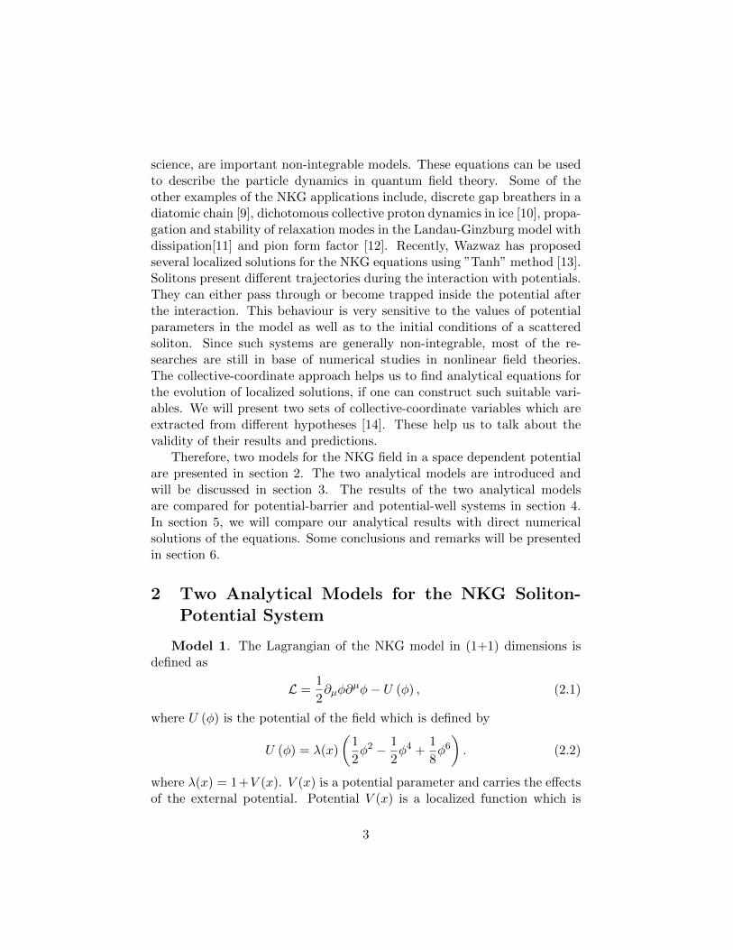
where X(t) = x0− Xt. Here, x0 and X are the soliton’s initial position and(constant) velocity, respectively. It is a kink-like solution as figure 1 shows.We intend to investigate the behaviour of kink solution (2.4) during the

Figure 1: Kink-like solution of the NKG described by equation (2.3) forx0 = 0 and X = 0.5 at t = 0.

interaction with an external potential using collective-coordinate technique.The derivation of the collective action for the motion of the vortex cen-

ters starts with the elegant idea of Manton [17]. A collective action canbe constructed by substituting the collective-vortex ansatz for the field con-figuration with vortices at Xi(t), i = 1, ..., N, into the effective field-theory

4

action and reduce the action to a function of the collective coordinates,L[Xi(t)] =

∫L (ψ (x, t,Xi(t))) [18]. It is clear that (2.4) is not the exact

solution for the equation (2.3). But it is approximate solution if V (x) is alocal weak perturbation [16].

By inserting the solution (2.4) in the Lagrangian (2.1) and using adia-batic approximation [2] we have

L =

(X2 − 1

)sech4 (x−X)

8 (1 + tanh (x−X))− λ(x)

8sech2 (x−X) (1− tanh (x−X)) .

(2.5)

In the adiabatic approximation one would suppose that the soliton veloc-ity changes in an adiabatic process. Therefore, the soliton speed changesvery slowly. Moreover, we have considered solitons with a small and slowlyvarying velocity.

Model 2. The general form of the action in an arbitrary metric is

S =

∫L(φ, ∂µφ)

√−gdnxdt, (2.6)

where ”g” is the determinant of the metric gµν(x). Therefore, we have aneffective Lagrangian Leff = L

√−g. The energy density of the system can be

calculated by varying both the field and the metric [6]. For the Lagrangianof the form (2.1) the equation of motion becomes [8, 14]

1√−g(√−g∂µ∂µφ+ ∂µφ∂

µ√−g)

+∂U(φ)

∂φ= 0. (2.7)

A space-dependent potential can be added to the Lagrangian of the systemby introducing a suitable nontrivial metric for the background space-time [6,14]. In other words, the metric carries the information about the potential.In the presence of a weak potential V (x) the suitable metric is [6, 8, 14]

gµν(x) ∼=(

1 + V (x) 00 −1

). (2.8)

By inserting the solution (2.4) in the effective Lagrangian (Leff ) with thepotential (2.2) of the NKG and using the metric (2.8), with adiabatic ap-proximation [2, 3], we have

Leff =√

1 + V (x)(

(1− V (x)) X2 − 1) sech4 ((x−X))

8 (1 + tanh (x−X))

−√

1 + V (x)

8sech2 (x−X) (1− tanh (x−X)) . (2.9)

5

For the weak potential V (x) (2.9) becomes

Leff ∼=((

1− V (x)

2

)X2 −

(1 +

V (x)

2

))sech4 ((x−X))

8 (1 + tanh (x−X))

−1 + V (x)

2

8sech2 (x−X) (1− tanh (x−X)) . (2.10)

3 Collective Coordinate for the two Models

The Lagrangian density of the soliton is described by (2.5) in model 1and (2.10) in model 2. These two equations are different in kinetic andalso potential terms. We will compare them later. The soliton internalstructure can be ommited by integrating the Lagrangian density (or Hamil-tonian density) with respect to the variable x. The integrated Lagrangianis called collective Lagrangian. After the integration, the soliton appears asa point-like particle; however, the effect of its extended nature still reflectsin the kinetic and also potential parts of the collective Lagrangian. Thedynamics of the point-like particle can be described by equations which arederived from collective Lagrangian. It is interesting to compare the resultsof the collective equations with those of direct numerical simulation of themain Lagrangian density. Let us derive the collective Lagrangian and thepoint-like particle equation of motion in the two models.

Model 1. By integrating Lagrangian (2.5) over the variable x , X(t)remains as a collective coordinate. If we take the potential V (x) = εδ(x),collective Lagrangian is derived from (2.5) as

L =1

4X2 − ε

8sech2 (X) (1 + tanh (X))− 1

2, (3.11)

where M0 = 12 is the rest mass of the soliton in this model. The effective

potential comes from equation (3.11) which is given by

U (φ) =ε

8sech2 (X) (1 + tanh (X)) +

1

2. (3.12)

The NKG solitons have a special and interesting situation which has notbeen observed in other fields. If we plot the effective potential as a functionof collective position (X), we will find that it has a spatial shift with respectto the origin. Figure 2(a) shows the effective potential as a function ofposition (X) for ε = 2. Simulations also confirm this finding for the NKGmodel. Figure 2(b) presents the shape of the potential barrier as seen by the

6

soliton which has been plotted using numerical calculation. It is a specialcharacteristic for the NKG field theory. The source of this distinction withrespect to other fields needs further consideration.

Figure 2: (a) Effective potential as a function of position with ε = 2. (b)Potential barrier as seen by the soliton in model 1 using numerical simula-tions.

The equation of motion for the variable X(t) is derived from (3.11) as

1

2X − ε

2sech2 (X)

[3

4tanh2 (X) +

1

2tanh (X)− 1

4

]= 0. (3.13)

We can define a collective force on the soliton if we look at the above equationas F = MX, where M is the rest mass of the soliton. Therefore, we have

F =ε

2sech2 (X)

[3

4tanh2 (X) +

1

2tanh (X)− 1

4

]. (3.14)

The above equation shows that the peak of the soliton moves under theinfluence of a complicated force which is a function of an external potentialand soliton position. Suppose that a soliton moves toward a potential bar-rier. Its velocity will reduce due to the effect of a repulsive force. While thesoliton is moving away, its velocity increases. Figures 3(a) and 3(b) showthe force exerted by the potential well and barrier on the soliton for ε = −4and ε = 4 respectively. This is in agreement with the observed behaviourfor the NKG model as shown in figure 2. These figures also show that thecenter of the force is not located in the origin.

7

Figure 3: (a) The force on the soliton by a potential well with ε = −4. (b)The force on the soliton by a barrier with ε = 4.

Interestingly, equation (3.13) has an exact solution for X as follows

X2 − X02

=ε

2[tanh3 (X) + tanh2 (X)− tanh (X)

− tanh3 (X0)− tanh2 (X0) + tanh (X0)], (3.15)

where X0 and X0 are the soliton’s initial position and initial velocity, re-spectively. Some of the physical features of a soliton-potential system canbe discovered using equation (3.15). Collective energy is obtainable fromLagrangian (3.11) as follows

E =1

4X2 +

ε

8sech2 (X) (1 + tanh (X)) +

1

2. (3.16)

It is the energy of a particle with the mass of M0 = 12 and the velocity

of X, where the particle moves under the influence of an external effectivepotential. By substituting X from (3.15) in the equation (3.16), it is shownthat the energy of the system is a function of soliton’s initial conditions X0

and X0 and therefore it is conserved.Model 2. The above results can be calculated using model 2. For the

Lagrangian (2.10) X(t) remains a collective coordinate if we integrate (2.10)over the variable x. If we take the potential V (x) = εδ(x), the collectiveLagrangian becomes

L =

(1

4− εsech4 (X)

16 (1− tanh (X))

)X2 − ε

8

(sech4(X)

1− tanh (X)

)− 1

2. (3.17)

8

The equation of motion for the variable X(t) is derived from (3.17):(1

2− εsech4 (X)

8 (1− tanh (X))

)X − ε

16sech2 (X)

×(−3 tanh2 (X)− 2 tanh (X) + 1

) (X2 − 2

)= 0. (3.18)

The above equation describes the soliton trajectory which moves under theinfluence of a collective force. The collective force is a function of the soli-ton’s position and velocity. X(t) can be calculated as a function of X(t) byintegrating (3.18) as follows

X2 − 2

X02 − 2

=1− εsech4(X0)

4(1−tanh(X0))

1− εsech4(X)4(1−tanh(X))

, (3.19)

where X0 and X0 are the soliton’s initial position and initial velocity, respec-tively. The energy of the soliton in the presence of the potential V (x) = εδ(x)using model 2 becomes

E =

(1

4− εsech4 (X)

16 (1− tanh (X))

)X2 +

ε

8

(sech4(X)

1− tanh (X)

)+

1

2. (3.20)

Equation (3.20) shows that the rest mass is a function of the soliton’s posi-tion in model 2. This is the source of some differences between the two mod-els which will be discussed in the next section. In section 4, some featuresof the soliton-potential dynamics are studied analytically using equations(3.19) and (3.20).

4 Comparing the Models

Potential barrier. There are two different trajectories for a solitonduring the interaction with an effective potential barrier which depend onthe soliton’s initial conditions. A soliton with a low velocity reflects backfrom the barrier and a high-velocity soliton climbs up the barrier and passesover it. So, these two situations can be distinguished by a critical velocity.The total energy of the soliton-potential is conserved in both models asmentioned before. Therefore, we can find the critical velocity with a simpleanalysis of the energy of the soliton without any numerical simulations. Both

equations (3.16) and (3.20) are reduced to E(X = ∞) = 14X0

2+ 1

2 whenthe soliton is far from the center of the delta-like potential which is located

9

at the origin. It is the energy of a particle with the mass of M0 = 12 and

velocity of X0. The energy of a soliton in the origin (X = 0) comes from

(3.16) and (3.20) for the two models: E1(X = 0) = 14X0

2+ ε

8 + 12 for model

1 and E2(X = 0) =(14 −

ε16

)X0

2+ ε

8 + 12 for model 2. The minimum energy

of soliton in this position is E = ε8 + 1

2 for the two models. On the otherhand, a soliton which comes from the infinity with initial velocity vc has theenergy of E = 1

4vc2 + 1

2 . So it is easy to calculate the critical velocity ofsoliton by comparing the energy of the soliton at the origin to its energy atinfinity. The critical velocity is calculated as vc =

√ε2 using both models.

The same result is derived by substituting X = 0 , X0 = vc , X0 = ∞ andX = 0 in (3.15) and (3.19).

Note that the critical velocity of a soliton depends on its initial positionas well as its initial velocity. For a soliton which is located at some positionlike X0 (which is not necessarily infinity) the critical velocity will not bevc =

√ε2 . So a soliton in the initial position X0 with initial velocity of X0

has the critical initial velocity if its velocity becomes zero at the top of thebarrier X = 0. Consider a soliton with initial conditions of X0 and X0. Ifwe set X = 0 and X = 0 in equations (3.15) and (3.19) then vc = X0. Thusfor model 1 we have

vc =

√− ε

2

(tanh (X0)− tanh2 (X0)− tanh3 (X0)

). (4.21)

But the critical velocity in model 2 becomes

vc =

√2ε(1− tanh(X0)− sech4(X0)

)4− 4 tanh(X0)− εsech4(X0)

. (4.22)

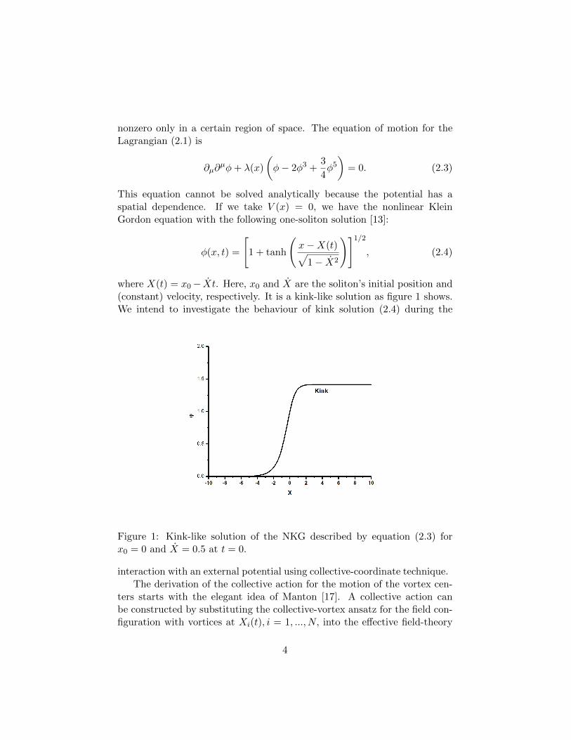
Figure 4 shows the critical velocity as a function of the potential strengthfor X0 = −1 in the two models. This figure shows that model 1 predictssmaller critical velocity compared to model 2 due to the differences betweenrest masses of these models. It is clear that a soliton with a great rest massneeds smaller velocity to reach the potential peak. The difference betweenthe rest mass of the soliton in model 1 and that of the soliton in model 2can be calculated using (3.16) and (3.20) as

4Ekinetic =εsech4(X)

16 (1− tanh(X))X2. (4.23)

The above equation shows that the two models predict equal rest mass atthe infinity. But the difference between the calculated rest mass in the two

10

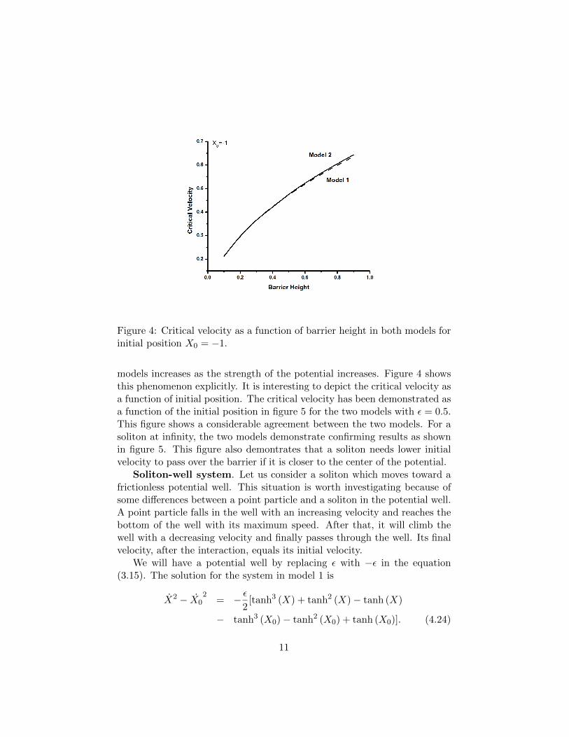
Figure 4: Critical velocity as a function of barrier height in both models forinitial position X0 = −1.

models increases as the strength of the potential increases. Figure 4 showsthis phenomenon explicitly. It is interesting to depict the critical velocity asa function of initial position. The critical velocity has been demonstrated asa function of the initial position in figure 5 for the two models with ε = 0.5.This figure shows a considerable agreement between the two models. For asoliton at infinity, the two models demonstrate confirming results as shownin figure 5. This figure also demontrates that a soliton needs lower initialvelocity to pass over the barrier if it is closer to the center of the potential.

Soliton-well system. Let us consider a soliton which moves toward africtionless potential well. This situation is worth investigating because ofsome differences between a point particle and a soliton in the potential well.A point particle falls in the well with an increasing velocity and reaches thebottom of the well with its maximum speed. After that, it will climb thewell with a decreasing velocity and finally passes through the well. Its finalvelocity, after the interaction, equals its initial velocity.

We will have a potential well by replacing ε with −ε in the equation(3.15). The solution for the system in model 1 is

X2 − X02

= − ε2

[tanh3 (X) + tanh2 (X)− tanh (X)

− tanh3 (X0)− tanh2 (X0) + tanh (X0)]. (4.24)

11

Figure 5: Critical velocity as a function of initial position in both modelsfor ε = 0.5.

Similary, for model 2 we have

X2 − 2

X02 − 2

=1 + εsech4(X0)

4(1−tanh(X0))

1 + εsech4(X)4(1−tanh(X))

. (4.25)

We can define an escape velocity instead of a critical velocity for a soliton-well system. The escape velocity is the minimum velocity for a solitonwhich can pass through a well. A soliton in an initial position X0 reachesthe infinity with a zero final velocity if its initial velocity is

Xescape1 =

√ε

2

(sech2 (X0)− tanh3 (X0) + tanh (X0)

), (4.26)

and

Xescape2 =

√2εsech4 (X0)

4− 4 tanh(X0) + εsech4(X0), (4.27)

which are calculated using models 1 and 2 respectively. In other words, asoliton which is located in the initial position X0 can escape to infinity ifits initial velocity X0 is greater than the escape velocity Xescape. Figures6 and 7 show the escape velocities from a potential well as a function of

12

the well depth (figure 6) and soliton’s initial position (figure 7) using thetwo models. Due to its bigger rest mass, the soliton in model 2 needs lowerescape velocity in comparison with the soliton in model 1. This is obviousin the equation (4.23).

Figure 6: Escape velocity as a function of the well depth in both models forinitial position X0 = −1.

Consider a soliton which moves toward the potential well with an initialvelocity X0 smaller than the escape velocity Xescape. The soliton reaches amaximum distance Xmax from the center of the potential with a zero velocityand then comes back toward the center of the potential well. Therefore, thesoliton oscillates in the well with the amplitude of Xmax. The required initialvelocity to reach Xmax is found from (4.25) for model 2 as

X0 =

√2ε(sech4X0 (1− tanhXmax)− sech4Xmax (1− tanhX0)

)(1− tanhXmax)

(4− 4 tanhX0 + εsech4X0

) . (4.28)

It is clear that the soliton oscillates around the well if its initial velocity islower than the escape velocity. The period of the oscillation can be calcu-lated numerically using equation (4.25).

13

Figure 7: Escape velocity as a function of initial position in both models forε = 0.5.

5 Analytical Results vs. Numerical Simulation

It is shown that the general behaviour of a soliton-potential system isalmost the same in models 1 and 2. However, we can find some small differ-ences between the dynamics of a soliton in the two models. It is importantto compare the results of analytical models to direct numerical solutions.Here, we will compare the analytic results of model 1 to its numerical so-lution. It is clear that the same comparison can be done for model 2. Thesoliton equation of motion for a small potential in model 1 is [18]

φtt − φxx + (1 + σδ(x))∂U

∂φ= 0. (5.29)

Both models (for a delta-like potential) have a parameter in their equationof motion which controls the strength of the external potential. It is possibleto compare the strength parameters in a specific situation by simulating andadjusting parameters in order to have the same results in different models forthat specific situation. It is expected to find approximately the same relationbetween the parameters in other situations. We found that the criticalvelocity for a soliton-barrier system is vc =

√ε2 . It is possible to adjust

the strength parameter ε in an analytical model with the same parameter in

14

(5.29) by means of vc. Numerical simulations using equation (5.29) show thesame behaviour for a critical velocity. An effective potential can be found

by interpolation of simulation results on the vc =√

εeff2 =

√α+εβ

2 . εeff is

the potential strength (as an effective parameter) in numerical simulationwhile ε is similar parameter in model 1. εeff can be found by fitting thenumerical results on a theoretical diagram as

εeffective = (0.0434± 0.01061) + (0.76462± 0.02479) ε. (5.30)

Figure 8 shows the result of simulations of equation (5.29) for the NKGmodel. Our simulations show a very good agreement between numericalresults and theoretical predictions for other features of soliton-potential in-teraction.

Figure 8: Critical velocity as a function of ε with results of simulation usingequation (5.29) and analytical model.

6 Conclusions and Remarks

Two analytical models for the interaction of the NKG solitons with deltafunction potential have been presented. The two models predict a criti-cal velocity for the soliton-barrier interaction which is a function of initialconditions and the potential identities. For a soliton-well system an escape

15

velocity has been introduced instead of the critical velocity. These mod-els are able to explain most of the features of the system analytically. Wehave observed that the center of the potential, as seen by the NKG solitons,is quite different from the real position of the potential center. Numeri-cal simulations are in agreement with theoretical predictions of the models.Our models fail to predict the narrow windows of soliton reflection fromthe potential well. So, it is expected to find a better model with a suitablecollective-coordinate method to explain this behaviour. These models canbe used to predict the soliton behaviour in the other field theories besidethe NKG model.

References

[1] Biaszak M. 1987 J. Phys. A: Math. Gen. 20 L1253-L1255

[2] Kivshar Y. S., Fei Z. and Vasquez L. 1991 Phys. Rev. Lett. 67 1177.

[3] Fei Z., Kivshar Y. S. and Vasquez L. 1992 Phys. Rev. A46 5214.

[4] Piette B., Zakrzewski W. J. and Brand J. 2005 J. Phys. A: Math. Gen.38 10403-10412.

[5] Piette B., Zakrzewski W. J. 2007 J. Phys. A: Math. Theor. 40 No 2,329-346.

[6] Kalbermann G. 1999 Phys. Lett A252 37-42

[7] Javidan K. 2006 J. Phys. A: Math. Gen. 39 No 33 10565-10574.

[8] Javidan K. 2008 Phys. Rev. E 78, 046607.

[9] A. V. Gorbach, M. Johansson, Phys. Rev. E 67, 066608 (2003).

[10] A. V. Zolotaryuk, A. V. Savin and E. N. Economou, Phys. Rev. B 57,234 (1998).

[11] M. Otwinowski, J. A. Tuszyski, and J. M. Dixon, Phys. Rev. A 45, 7263(1992).

[12] M. Bawin, M. Jaminon, Phys. Rev. C 30 (1) (1984) 331-334.

[13] Wazwaz A. M. (2006) Chaos, solitons and fractals 28 1005-1013.

[14] Saadatmand D., Javidan K. Phys. Scr. 85 (2012) 025003.

[15] N. S. Manton, Phys. Lett. B 110, 54 (1982).

[16] F. Lund, Phys. Lett. A 159, 245 (1991).

[17] Javidan K. Journal of Mathematical Physics 51, 112902 (2010).

[18] Al-Alawi Jassem H., Zakrzewski W. J. (2007) J. Phys. A 40, 11319.

16