bodenseo

Data Analysis

Numpy, Matplotlib and Pandas

byBernd Klein

© 2021 Bernd Klein

All rights reserved. No portion of this book may be reproduced or used in any manner without written permission from the copyright owner.

For more information, contact address: bernd.klein@python-course.eu

www.python-course.eu

Python CourseData Analysis With

Python by BerndKlein

Numpy Tutorial ..........................................................................................................................8Numpy Tutorial: Creating Arrays.............................................................................................17Data Type Objects, dtype..........................................................................................................36Numerical Operations on Numpy Arrays.................................................................................48Numpy Arrays: Concatenating, Flattening and Adding Dimensions .......................................68Python, Random Numbers and Probability ..............................................................................79Weighted Probabilities..............................................................................................................90Synthetical Test Data With Python.........................................................................................119Numpy: Boolean Indexing......................................................................................................136Matrix Multiplicaion, Dot and Cross Product ........................................................................143Reading and Writing Data Files .............................................................................................149Overview of Matplotlib ..........................................................................................................157Format Plots............................................................................................................................168Matplotlib Tutorial..................................................................................................................172Shading Regions with fill_between() .....................................................................................183Matplotlib Tutorial: Spines and Ticks ....................................................................................186Matplotlib Tutorial, Adding Legends and Annotations..........................................................197Matplotlib Tutorial: Subplots .................................................................................................212Exercise ....................................................................................................................................44Exercise ....................................................................................................................................44Matplotlib Tutorial: Gridspec .................................................................................................239GridSpec using SubplotSpec ..................................................................................................244Matplotlib Tutorial: Histograms and Bar Plots ......................................................................248Matplotlib Tutorial: Contour Plots .........................................................................................268Introduction into Pandas.........................................................................................................303Data Structures .......................................................................................................................305Accessing and Changing values of DataFrames.....................................................................343Pandas: groupby .....................................................................................................................361Reading and Writing Data ......................................................................................................380Dealing with NaN...................................................................................................................394

Binning in Python and Pandas................................................................................................404Expenses and Income Example ..............................................................................................465Net Income Method Example.................................................................................................478

3

N U M E R I C A L P R O G R A M M I N G W I T HP Y T H O N

NUMERICAL PROGRAMMING DEFINITION

The term "Numerical Computing" - a.k.a. numerical computing or scientific computing - can be misleading.One can think about it as "having to do with numbers" as opposed to algorithms dealing with texts forexample. If you think of Google and the way it provides links to websites for your search inquiries, you maythink about the underlying algorithm as a text based one. Yet, the core of the Google search engine isnumerical. To perform the PageRank algorithm Google executes the world's largest matrix computation.

Numerical Computing defines an area of computer science and mathematics dealing with algorithms fornumerical approximations of problems from mathematical or numerical analysis, in other words: Algorithmssolving problems involving continuous variables. Numerical analysis is used to solve science and engineeringproblems.

DATA SCIENCE AND DATA ANALYSIS

This tutorial can be used as an online course on Numerical Python as it is needed by Data Scientists and DataAnalysts.

Data science is an interdisciplinary subject which includes for example statistics and computer science,especially programming and problem solving skills. Data Science includes everything which is necessary tocreate and prepare data, to manipulate, filter and clense data and to analyse data. Data can be both structuredand unstructured. We could also say Data Science includes all the techniques needed to extract and gaininformation and insight from data.

Data Science is an umpbrella term which incorporates data analysis, statistics, machine learning and otherrelated scientific fields in order to understand and analyze data.

Another term occuring quite often in this context is "Big Data". Big Data is for sure one of the most often usedbuzzwords in the software-related marketing world. Marketing managers have found out that using this termcan boost the sales of their products, regardless of the fact if they are really dealing with big data or not. Theterm is often used in fuzzy ways.

Big data is data which is too large and complex, so that it is hard for data-processing application software todeal with them. The problems include capturing and collecting data, data storage, search the data, visualizationof the data, querying, and so on.

The following concepts are associated with big data:

• volume:the sheer amount of data, whether it will be giga-, tera-, peta- or exabytes

• velocity:the speed of arrival and processing of data

• veracity:

4

uncertainty or imprecision of data• variety:

the many sources and types of data both structured and unstructured

The big question is how useful Python is for these purposes. If we would only use Python without any specialmodules, this language could only poorly perform on the previously mentioned tasks. We will describe thenecessary tools in the following chapter.

CONNECTIONS BETWEEN PYTHON, NUMPY, MATPLOTLIB, SCIPY ANDPANDAS

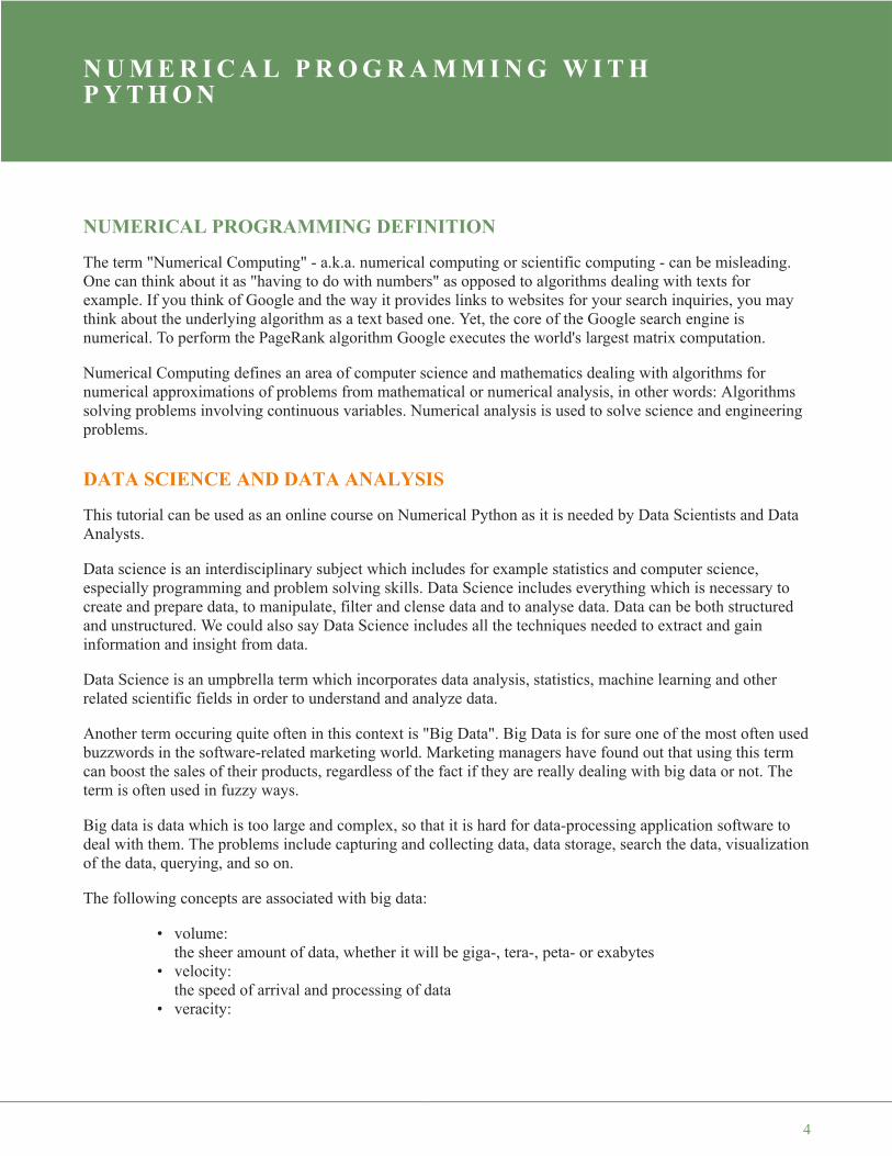
Python is a general-purpose language and as such it can and it iswidely used by system administrators for operating systemadministration, by web developpers as a tool to create dynamicwebsites and by linguists for natural language processing tasks.Being a truely general-purpose language, Python can of course -without using any special numerical modules - be used to solvenumerical problems as well. So far so good, but the crux of thematter is the execution speed. Pure Python without anynumerical modules couldn't be used for numerical tasks Matlab,R and other languages are designed for. If it comes tocomputational problem solving, it is of greatest importance toconsider the performance of algorithms, both concerning speedand data usage.

If we use Python in combination with its modules NumPy,SciPy, Matplotlib and Pandas, it belongs to the top numericalprogramming languages. It is as efficient - if not even moreefficient - than Matlab or R.

5

Numpy is a module which provides the basic data structures,implementing multi-dimensional arrays and matrices. Besidesthat the module supplies the necessary functionalities to createand manipulate these data structures. SciPy is based on top ofNumpy, i.e. it uses the data structures provided by NumPy. Itextends the capabilities of NumPy with further useful functionsfor minimization, regression, Fourier-transformation and manyothers.

Matplotlib is a plotting library for the Python programminglanguage and the numerically oriented modules like NumPy andSciPy.

The youngest child in this family of modules is Pandas. Pandasis using all of the previously mentioned modules. It's build ontop of them to provide a module for the Python language, whichis also capable of data manipulation and analysis. The specialfocus of Pandas consists in offering data structures andoperations for manipulating numerical tables and time series. The name is derived from the term "panel data".Pandas is well suited for working with tabular data as it is known from spread sheet programming like Excel.

PYTHON, AN ALTERNATIVE TO MATLAB

Python is becoming more and more the main programming language for data scientists. Yet, there are stillmany scientists and engineers in the scientific and engineering world that use R and MATLAB to solve theirdata analysis and data science problems. It's a question troubling lots of people, which language they shouldchoose: The functionality of R was developed with statisticians in mind, whereas Python is a general-purposelanguage. Nevertheless, Python is also - in combination with its specialized modules, like Numpy, Scipy,Matplotlib, Pandas and so, - an ideal programming language for solving numerical problems. Furthermore, thecommunity of Python is a lot larger and faster growing than the one from R.

The principal disadvantage of MATLAB against Python are the costs. Python with NumPy, SciPy, Matplotliband Pandas is completely free, whereas MATLAB can be very expensive. "Free" means both "free" as in "freebeer" and "free" as in "freedom"! Even though MATLAB has a huge number of additional toolboxes available,Python has the advantage that it is a more modern and complete programming language. Python is continuallybecoming more powerful by a rapidly growing number of specialized modules.

Python in combination with Numpy, Scipy, Matplotlib and Pandas can be used as a complete replacement forMATLAB.

6

7

N U M P Y T U T O R I A L

INTRODUCTION

NumPy is a module for Python. The name is an acronym for"Numeric Python" or "Numerical Python". It is pronounced/ˈnʌmpaɪ/ (NUM-py) or less often /ˈnʌmpi (NUM-pee)). It is anextension module for Python, mostly written in C. This makessure that the precompiled mathematical and numerical functionsand functionalities of Numpy guarantee great execution speed.

Furthermore, NumPy enriches the programming languagePython with powerful data structures, implementing multi-dimensional arrays and matrices. These data structuresguarantee efficient calculations with matrices and arrays. Theimplementation is even aiming at huge matrices and arrays,better know under the heading of "big data". Besides that themodule supplies a large library of high-level mathematical functions to operate on these matrices and arrays.

SciPy (Scientific Python) is often mentioned in the same breath with NumPy. SciPy needs Numpy, as it isbased on the data structures of Numpy and furthermore its basic creation and manipulation functions. Itextends the capabilities of NumPy with further useful functions for minimization, regression, Fourier-transformation and many others.

Both NumPy and SciPy are not part of a basic Python installation. They have to be installed after the Pythoninstallation. NumPy has to be installed before installing SciPy.

(Comment: The diagram of the image on the right side is the graphical visualisation of a matrix with 14 rowsand 20 columns. It's a so-called Hinton diagram. The size of a square within this diagram corresponds to thesize of the value of the depicted matrix. The colour determines, if the value is positive or negative. In ourexample: the colour red denotes negative values and the colour green denotes positive values.)

NumPy is based on two earlier Python modules dealing with arrays. One of these is Numeric. Numeric is likeNumPy a Python module for high-performance, numeric computing, but it is obsolete nowadays. Anotherpredecessor of NumPy is Numarray, which is a complete rewrite of Numeric but is deprecated as well. NumPyis a merger of those two, i.e. it is build on the code of Numeric and the features of Numarray.

COMPARISON BETWEEN CORE PYTHON AND NUMPY

8

Let's assume, we want to turn the values into degrees Fahrenheit. This is very easy to accomplish with anumpy array. The solution to our problem can be achieved by simple scalar multiplication:

When we say "Core Python", we mean Python without any special modules, i.e. especially without NumPy.

The advantages of Core Python:

• high-level number objects: integers, floating point• containers: lists with cheap insertion and append methods, dictionaries with fast lookup

Advantages of using Numpy with Python:

• array oriented computing• efficiently implemented multi-dimensional arrays• designed for scientific computation

A SIMPLE NUMPY EXAMPLE

Before we can use NumPy we will have to import it. It has to be imported like any other module:

import numpy

But you will hardly ever see this. Numpy is usually renamed to np:

import numpy as np

Our first simple Numpy example deals with temperatures. Given is a list with values, e.g. temperatures inCelsius:

cvalues = [20.1, 20.8, 21.9, 22.5, 22.7, 22.3, 21.8, 21.2, 20.9, 20.1]

We will turn our list "cvalues" into a one-dimensional numpy array:

C = np.array(cvalues)print(C)

print(C * 9 / 5 + 32)

[20.1 20.8 21.9 22.5 22.7 22.3 21.8 21.2 20.9 20.1]

[68.18 69.44 71.42 72.5 72.86 72.14 71.24 70.16 69.62 68.18]

9

The array C has not been changed by this expression:

print(C)

Compared to this, the solution for our Python list looks awkward:

fvalues = [ x*9/5 + 32 for x in cvalues]print(fvalues)

So far, we referred to C as an array. The internal type is "ndarray" or to be even more precise "C is an instanceof the class numpy.ndarray":

type(C)

In the following, we will use the terms "array" and "ndarray" in most cases synonymously.

GRAPHICAL REPRESENTATION OF THE VALUES

Even though we want to cover the module matplotlib not until a later chapter, we want to demonstrate how wecan use this module to depict our temperature values. To do this, we us the package pyplot from matplotlib.

If you use the jupyter notebook, you might be well advised to include the following line of code to prevent anexternal window to pop up and to have your diagram included in the notebook:

%matplotlib inline

The code to generate a plot for our values looks like this:

import matplotlib.pyplot as pltplt.plot(C)plt.show()

[20.1 20.8 21.9 22.5 22.7 22.3 21.8 21.2 20.9 20.1]

[68.18, 69.44, 71.42, 72.5, 72.86, 72.14, 71.24000000000001, 70.16, 69.62, 68.18]

Output: numpy.ndarray

10

The function plot uses the values of the array C for the values of the ordinate, i.e. the y-axis. The indices of thearray C are taken as values for the abscissa, i.e. the x-axis.

MEMORY CONSUMPTION: NDARRAY AND LIST

The main benefits of using numpy arrays should be smaller memory consumption and better runtimebehaviour. We want to look at the memory usage of numpy arrays in this subchapter of our turorial andcompare it to the memory consumption of Python lists.

11

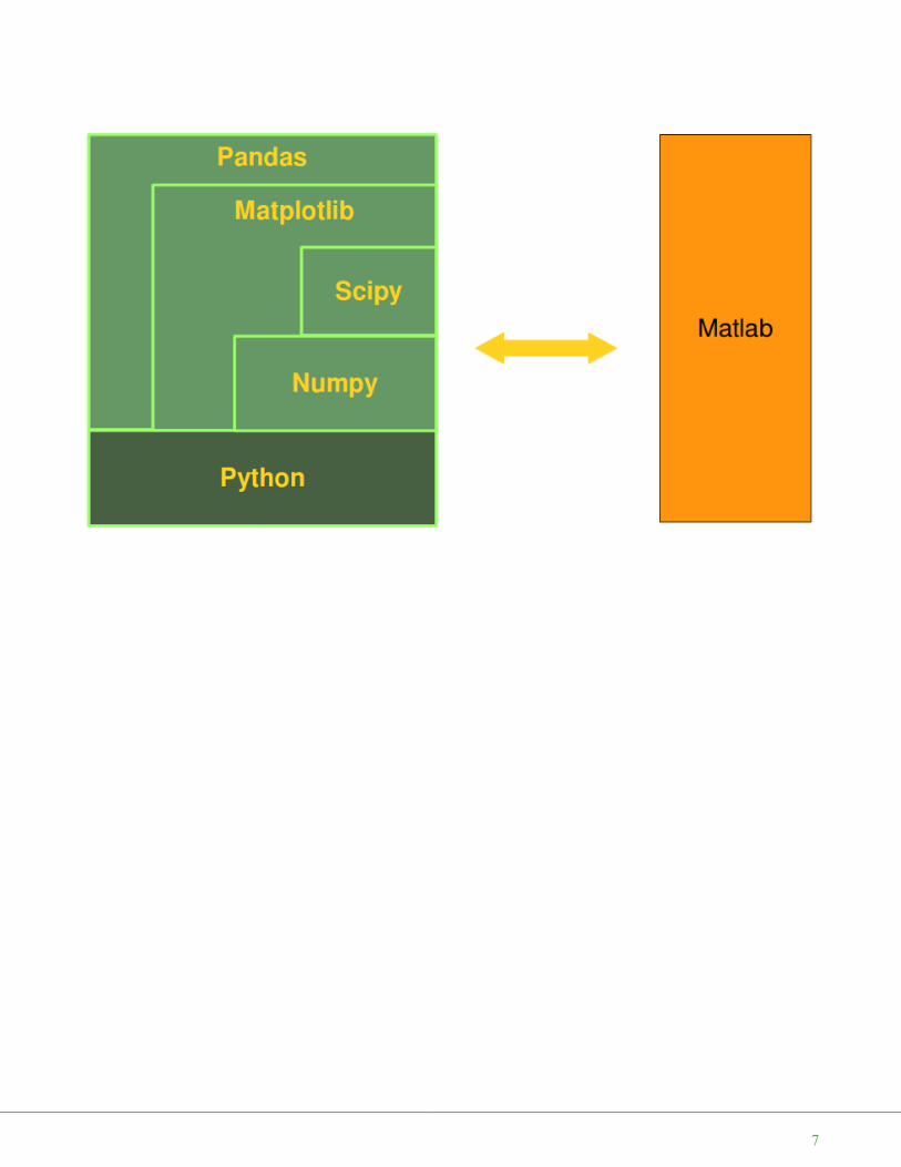
To calculate the memory consumption of the list from the above picture, we will use the function getsizeoffrom the module sys.

from sys import getsizeof as size

lst = [24, 12, 57]

size_of_list_object = size(lst) # only green boxsize_of_elements = len(lst) * size(lst[0]) # 24, 12, 57

total_list_size = size_of_list_object + size_of_elementsprint("Size without the size of the elements: ", size_of_list_object)print("Size of all the elements: ", size_of_elements)print("Total size of list, including elements: ", total_list_size)

The size of a Python list consists of the general list information, the size needed for the references to theelements and the size of all the elements of the list. If we apply sys.getsizeof to a list, we get only the sizewithout the size of the elements. In the previous example, we made the assumption that all the integerelements of our list have the same size. Of course, this is not valid in general, because memory consumptionwill be higher for larger integers.

We will check now, how the memory usage changes, if we add another integer element to the list. We alsolook at an empty list:

lst = [24, 12, 57, 42]

size_of_list_object = size(lst) # only green boxsize_of_elements = len(lst) * size(lst[0]) # 24, 12, 57, 42

total_list_size = size_of_list_object + size_of_elementsprint("Size without the size of the elements: ", size_of_list_object)print("Size of all the elements: ", size_of_elements)print("Total size of list, including elements: ", total_list_size)

lst = []print("Emtpy list size: ", size(lst))

Size without the size of the elements: 96Size of all the elements: 84Total size of list, including elements: 180

12

We can conclude from this that for every new element, we need another eight bytes for the reference to thenew object. The new integer object itself consumes 28 bytes. The size of a list "lst" without the size of theelements can be calculated with:

64 + 8 * len(lst)

To get the complete size of an arbitrary list of integers, we have to add the sum of all the sizes of the integers.

We will examine now the memory consumption of a numpy.array. To this purpose, we will have a look at theimplementation in the following picture:

We will create the numpy array of the previous diagram and calculate the memory usage:

a = np.array([24, 12, 57])print(size(a))

We get the memory usage for the general array information by creating an empty array:

e = np.array([])print(size(e))

Size without the size of the elements: 104Size of all the elements: 112Total size of list, including elements: 216Emtpy list size: 72

120

96

13

We can see that the difference between the empty array "e" and the array "a" with three integers consists in 24Bytes. This means that an arbitrary integer array of length "n" in numpy needs

96 + n * 8 Bytes

whereas a list of integers needs, as we have seen before

64 + 8 len(lst) + len(lst) 28

This is a minimum estimation, as Python integers can use more than 28 bytes.

When we define a Numpy array, numpy automatically chooses a fixed integer size. In our example "int64".We can determine the size of the integers, when we define an array. Needless to say, this changes the memoryrequirement:

a = np.array([24, 12, 57], np.int8)print(size(a) - 96)

a = np.array([24, 12, 57], np.int16)print(size(a) - 96)

a = np.array([24, 12, 57], np.int32)print(size(a) - 96)

a = np.array([24, 12, 57], np.int64)print(size(a) - 96)

TIME COMPARISON BETWEEN PYTHON LISTS AND NUMPY ARRAYS

One of the main advantages of NumPy is its advantage in time compared to standard Python. Let's look at thefollowing functions:

import timesize_of_vec = 1000

def pure_python_version():t1 = time.time()

361224

14

X = range(size_of_vec)Y = range(size_of_vec)Z = [X[i] + Y[i] for i in range(len(X)) ]return time.time() - t1

def numpy_version():t1 = time.time()X = np.arange(size_of_vec)Y = np.arange(size_of_vec)Z = X + Yreturn time.time() - t1

Let's call these functions and see the time consumption:

t1 = pure_python_version()t2 = numpy_version()

print(t1, t2)print("Numpy is in this example " + str(t1/t2) + " faster!")

It's an easier and above all better way to measure the times by using the timeit module. We will use the Timerclass in the following script.

The constructor of a Timer object takes a statement to be timed, an additional statement used for setup, and atimer function. Both statements default to 'pass'.

The statements may contain newlines, as long as they don't contain multi-line string literals.

A Timer object has a timeit method. timeit is called with a parameter number:

timeit(number=1000000)

The main statement will be executed "number" times. This executes the setup statement once, and then returnsthe time it takes to execute the main statement a "number" of times. It returns the time in seconds.

import numpy as npfrom timeit import Timer

size_of_vec = 1000

X_list = range(size_of_vec)Y_list = range(size_of_vec)

0.0010614395141601562 5.2928924560546875e-05Numpy is in this example 20.054054054054053 faster!

15

X = np.arange(size_of_vec)Y = np.arange(size_of_vec)

def pure_python_version():Z = [X_list[i] + Y_list[i] for i in range(len(X_list)) ]

def numpy_version():Z = X + Y

#timer_obj = Timer("x = x + 1", "x = 0")timer_obj1 = Timer("pure_python_version()",

"from __main__ import pure_python_version")timer_obj2 = Timer("numpy_version()",

"from __main__ import numpy_version")

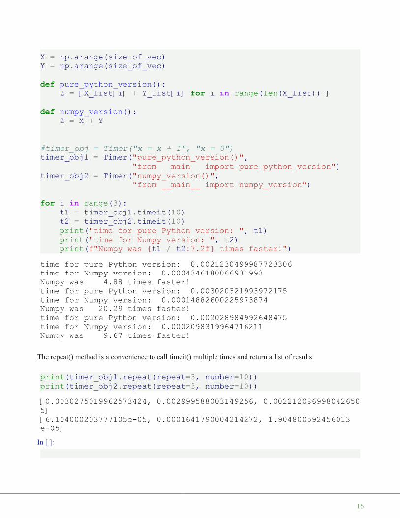
for i in range(3):t1 = timer_obj1.timeit(10)t2 = timer_obj2.timeit(10)print("time for pure Python version: ", t1)print("time for Numpy version: ", t2)print(f"Numpy was {t1 / t2:7.2f} times faster!")

The repeat() method is a convenience to call timeit() multiple times and return a list of results:

print(timer_obj1.repeat(repeat=3, number=10))print(timer_obj2.repeat(repeat=3, number=10))

In [ ]:

time for pure Python version: 0.0021230499987723306time for Numpy version: 0.0004346180066931993Numpy was 4.88 times faster!time for pure Python version: 0.003020321993972175time for Numpy version: 0.00014882600225973874Numpy was 20.29 times faster!time for pure Python version: 0.002028984992648475time for Numpy version: 0.0002098319964716211Numpy was 9.67 times faster!

[0.0030275019962573424, 0.002999588003149256, 0.0022120869980426505][6.104000203777105e-05, 0.0001641790004214272, 1.904800592456013e-05]

16

N U M P Y T U T O R I A L : C R E A T I N G A R R A Y S

We have alreday seen in the previous chapter of our Numpytutorial that we can create Numpy arrays from lists and tuples.We want to introduce now further functions for creating basicarrays.

There are functions provided by Numpy to create arrays withevenly spaced values within a given interval. One 'arange' uses agiven distance and the other one 'linspace' needs the number ofelements and creates the distance automatically.

CREATION OF ARRAYS WITH EVENLY SPACED VALUES

ARANGE

The syntax of arange:

arange([start,] stop[, step], [, dtype=None])

arange returns evenly spaced values within a given interval. The values are generated within the half-openinterval '[start, stop)' If the function is used with integers, it is nearly equivalent to the Python built-in functionrange, but arange returns an ndarray rather than a list iterator as range does. If the 'start' parameter is not given,it will be set to 0. The end of the interval is determined by the parameter 'stop'. Usually, the interval will notinclude this value, except in some cases where 'step' is not an integer and floating point round-off affects thelength of output ndarray. The spacing between two adjacent values of the output array is set with the optionalparameter 'step'. The default value for 'step' is 1. If the parameter 'step' is given, the 'start' parameter cannot beoptional, i.e. it has to be given as well. The type of the output array can be specified with the parameter 'dtype'.If it is not given, the type will be automatically inferred from the other input arguments.

import numpy as npa = np.arange(1, 10)print(a)

x = range(1, 10)

17

print(x) # x is an iteratorprint(list(x))

# further arange examples:x = np.arange(10.4)print(x)x = np.arange(0.5, 10.4, 0.8)print(x)

Be careful, if you use a float value for the step parameter, as you can see in the following example:

np.arange(12.04, 12.84, 0.08)

The help of arange has to say the following for the stop parameter: "End of interval. The interval doesnot include this value, except in some cases where step is not an integer and floating point round-offaffects the length of out . This is what happened in our example.

The following usages of arange is a bit offbeat. Why should we use float values, if we want integers asresult. Anyway, the result might be confusing. Before arange starts, it will round the start value, end value andthe stepsize:

x = np.arange(0.5, 10.4, 0.8, int)print(x)

This result defies all logical explanations. A look at help also helps here: "When using a non-integer step, suchas 0.1, the results will often not be consistent. It is better to use numpy.linspace for these cases. Usinglinspace is not an easy workaround in some situations, because the number of values has to be known.

[1 2 3 4 5 6 7 8 9]range(1, 10)[1, 2, 3, 4, 5, 6, 7, 8, 9][ 0. 1. 2. 3. 4. 5. 6. 7. 8. 9. 10.][ 0.5 1.3 2.1 2.9 3.7 4.5 5.3 6.1 6.9 7.7 8.5 9.3 10.1]

Output: array([12.04, 12.12, 12.2 , 12.28, 12.36, 12.44, 12.52, 12.6, 12.68,

12.76, 12.84])

[ 0 1 2 3 4 5 6 7 8 9 10 11 12]

18

LINSPACE

The syntax of linspace:

linspace(start, stop, num=50, endpoint=True, retstep=False)

linspace returns an ndarray, consisting of 'num' equally spaced samples in the closed interval [start, stop] or thehalf-open interval [start, stop). If a closed or a half-open interval will be returned, depends on whether'endpoint' is True or False. The parameter 'start' defines the start value of the sequence which will be created.'stop' will the end value of the sequence, unless 'endpoint' is set to False. In the latter case, the resultingsequence will consist of all but the last of 'num + 1' evenly spaced samples. This means that 'stop' is excluded.Note that the step size changes when 'endpoint' is False. The number of samples to be generated can be setwith 'num', which defaults to 50. If the optional parameter 'endpoint' is set to True (the default), 'stop' will bethe last sample of the sequence. Otherwise, it is not included.

import numpy as np# 50 values between 1 and 10:print(np.linspace(1, 10))# 7 values between 1 and 10:print(np.linspace(1, 10, 7))# excluding the endpoint:print(np.linspace(1, 10, 7, endpoint=False))[ 1. 1.18367347 1.36734694 1.55102041 1.73469388 1.91836735

2.10204082 2.28571429 2.46938776 2.65306122 2.83673469 3.02040816

3.20408163 3.3877551 3.57142857 3.75510204 3.93877551 4.12244898

4.30612245 4.48979592 4.67346939 4.85714286 5.04081633 5.2244898

5.40816327 5.59183673 5.7755102 5.95918367 6.14285714 6.32653061

6.51020408 6.69387755 6.87755102 7.06122449 7.24489796 7.42857143

7.6122449 7.79591837 7.97959184 8.16326531 8.34693878 8.53061224

8.71428571 8.89795918 9.08163265 9.26530612 9.44897959 9.63265306

9.81632653 10. ][ 1. 2.5 4. 5.5 7. 8.5 10. ][1. 2.28571429 3.57142857 4.85714286 6.14285714 7.428571438.71428571]

19

We haven't discussed one interesting parameter so far. If the optional parameter 'retstep' is set, the functionwill also return the value of the spacing between adjacent values. So, the function will return a tuple('samples', 'step'):

import numpy as npsamples, spacing = np.linspace(1, 10, retstep=True)print(spacing)samples, spacing = np.linspace(1, 10, 20, endpoint=True, retstep=True)print(spacing)samples, spacing = np.linspace(1, 10, 20, endpoint=False, retstep=True)print(spacing)

ZERO-DIMENSIONAL ARRAYS IN NUMPY

It's possible to create multidimensional arrays in numpy. Scalars are zero dimensional. In the followingexample, we will create the scalar 42. Applying the ndim method to our scalar, we get the dimension of thearray. We can also see that the type is a "numpy.ndarray" type.

import numpy as npx = np.array(42)print("x: ", x)print("The type of x: ", type(x))print("The dimension of x:", np.ndim(x))

ONE-DIMENSIONAL ARRAYS

We have already encountered a 1-dimenional array - better known to some as vectors - in our initial example.What we have not mentioned so far, but what you may have assumed, is the fact that numpy arrays arecontainers of items of the same type, e.g. only integers. The homogenous type of the array can be determinedwith the attribute "dtype", as we can learn from the following example:

F = np.array([1, 1, 2, 3, 5, 8, 13, 21])V = np.array([3.4, 6.9, 99.8, 12.8])

0.18367346938775510.473684210526315760.45

x: 42The type of x: <class 'numpy.ndarray'>The dimension of x: 0

20

print("F: ", F)print("V: ", V)print("Type of F: ", F.dtype)print("Type of V: ", V.dtype)print("Dimension of F: ", np.ndim(F))print("Dimension of V: ", np.ndim(V))

TWO- AND MULTIDIMENSIONAL ARRAYS

Of course, arrays of NumPy are not limited to one dimension. They are of arbitrary dimension. We create themby passing nested lists (or tuples) to the array method of numpy.

A = np.array([ [3.4, 8.7, 9.9],[1.1, -7.8, -0.7],[4.1, 12.3, 4.8]])

print(A)print(A.ndim)

B = np.array([ [[111, 112], [121, 122]],[[211, 212], [221, 222]],[[311, 312], [321, 322]] ])

print(B)print(B.ndim)

F: [ 1 1 2 3 5 8 13 21]V: [ 3.4 6.9 99.8 12.8]Type of F: int64Type of V: float64Dimension of F: 1Dimension of V: 1

[[ 3.4 8.7 9.9][ 1.1 -7.8 -0.7][ 4.1 12.3 4.8]]

2

[[[111 112][121 122]]

[[211 212][221 222]]

[[311 312][321 322]]]

3

21

SHAPE OF AN ARRAY

The function "shape" returns the shape of an array. The shape is a tuple ofintegers. These numbers denote the lengths of the corresponding arraydimension. In other words: The "shape" of an array is a tuple with the numberof elements per axis (dimension). In our example, the shape is equal to (6, 3),i.e. we have 6 lines and 3 columns.

x = np.array([ [67, 63, 87],[77, 69, 59],[85, 87, 99],[79, 72, 71],[63, 89, 93],[68, 92, 78]])

print(np.shape(x))

There is also an equivalent array property:

print(x.shape)

The shape of an array tells us also something about the order in which the indicesare processed, i.e. first rows, then columns and after that the further dimensions.

"shape" can also be used to change the shape of an array.

x.shape = (3, 6)print(x)

x.shape = (2, 9)print(x)

(6, 3)

(6, 3)

[[67 63 87 77 69 59][85 87 99 79 72 71][63 89 93 68 92 78]]

22

You might have guessed by now that the new shape must correspond to the number of elements of the array,i.e. the total size of the new array must be the same as the old one. We will raise an exception, if this is not thecase.

Let's look at some further examples.

The shape of a scalar is an empty tuple:

x = np.array(11)print(np.shape(x))

B = np.array([ [[111, 112, 113], [121, 122, 123]],[[211, 212, 213], [221, 222, 223]],[[311, 312, 313], [321, 322, 323]],[[411, 412, 413], [421, 422, 423]] ])

print(B.shape)

INDEXING AND SLICING

Assigning to and accessing the elements of an array is similar to other sequential data types of Python, i.e. listsand tuples. We have also many options to indexing, which makes indexing in Numpy very powerful andsimilar to the indexing of lists and tuples.

Single indexing behaves the way, you will most probably expect it:

F = np.array([1, 1, 2, 3, 5, 8, 13, 21])# print the first element of Fprint(F[0])# print the last element of Fprint(F[-1])

[[67 63 87 77 69 59 85 87 99][79 72 71 63 89 93 68 92 78]]

()

(4, 2, 3)

121

23

Indexing multidimensional arrays:

A = np.array([ [3.4, 8.7, 9.9],[1.1, -7.8, -0.7],[4.1, 12.3, 4.8]])

print(A[1][0])

We accessed an element in the second row, i.e. the row with the index 1, and the first column (index 0). Weaccessed it the same way, we would have done with an element of a nested Python list.

You have to be aware of the fact, that way of accessing multi-dimensional arrays can be highly inefficient. Thereason is that we create an intermediate array A[1] from which we access the element with the index 0. So itbehaves similar to this:

tmp = A[1]print(tmp)print(tmp[0])

There is another way to access elements of multi-dimensional arrays in Numpy: We use only one pair ofsquare brackets and all the indices are separated by commas:

print(A[1, 0])

We assume that you are familar with the slicing of lists and tuples. The syntax is the same in numpy for one-dimensional arrays, but it can be applied to multiple dimensions as well.

The general syntax for a one-dimensional array A looks like this:

A[start:stop:step]

We illustrate the operating principle of "slicing" with some examples. We start with the easiest case, i.e. theslicing of a one-dimensional array:

S = np.array([0, 1, 2, 3, 4, 5, 6, 7, 8, 9])print(S[2:5])print(S[:4])print(S[6:])

1.1

[ 1.1 -7.8 -0.7]1.1

1.1

24

print(S[:])

We will illustrate the multidimensional slicing in the following examples. The ranges for each dimension areseparated by commas:

A = np.array([[11, 12, 13, 14, 15],[21, 22, 23, 24, 25],[31, 32, 33, 34, 35],[41, 42, 43, 44, 45],[51, 52, 53, 54, 55]])

print(A[:3, 2:])

print(A[3:, :])

[2 3 4][0 1 2 3][6 7 8 9][0 1 2 3 4 5 6 7 8 9]

[[13 14 15][23 24 25][33 34 35]]

[[41 42 43 44 45][51 52 53 54 55]]

25

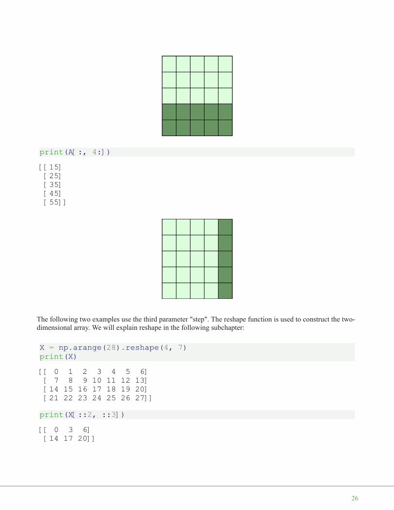
print(A[:, 4:])

The following two examples use the third parameter "step". The reshape function is used to construct the two-dimensional array. We will explain reshape in the following subchapter:

X = np.arange(28).reshape(4, 7)print(X)

print(X[::2, ::3])

[[15][25][35][45][55]]

[[ 0 1 2 3 4 5 6][ 7 8 9 10 11 12 13][14 15 16 17 18 19 20][21 22 23 24 25 26 27]]

[[ 0 3 6][14 17 20]]

26

print(X[::, ::3])

If the number of objects in the selection tuple is less than the dimension N, then : is assumedfor any subsequent dimensions:

A = np.array([ [ [45, 12, 4], [45, 13, 5], [46, 12, 6] ],

[ [46, 14, 4], [45, 14, 5], [46, 11, 5] ],[ [47, 13, 2], [48, 15, 5], [52, 15, 1] ] ])

A[1:3, 0:2] # equivalent to A[1:3, 0:2, :]

[[ 0 3 6][ 7 10 13][14 17 20][21 24 27]]

Output: array([[[46, 14, 4],[45, 14, 5]],

[[47, 13, 2],[48, 15, 5]]])

27

Attention: Whereas slicings on lists and tuples create new objects, a slicing operation on an array creates aview on the original array. So we get an another possibility to access the array, or better a part of the array.From this follows that if we modify a view, the original array will be modified as well.

A = np.array([0, 1, 2, 3, 4, 5, 6, 7, 8, 9])S = A[2:6]S[0] = 22S[1] = 23print(A)

Doing the similar thing with lists, we can see that we get a copy:

lst = [0, 1, 2, 3, 4, 5, 6, 7, 8, 9]lst2 = lst[2:6]lst2[0] = 22lst2[1] = 23print(lst)

If you want to check, if two array names share the same memory block, you can use the functionnp.may_share_memory.

np.may_share_memory(A, B)

To determine if two arrays A and B can share memory the memory-bounds of A and B are computed. Thefunction returns True, if they overlap and False otherwise. The function may give false positives, i.e. if itreturns True it just means that the arrays may be the same.

np.may_share_memory(A, S)

The following code shows a case, in which the use of may_share_memory is quite useful:

A = np.arange(12)B = A.reshape(3, 4)A[0] = 42print(B)

[ 0 1 22 23 4 5 6 7 8 9]

[0, 1, 2, 3, 4, 5, 6, 7, 8, 9]

Output: True

[[42 1 2 3][ 4 5 6 7][ 8 9 10 11]]

28

We can see that A and B share the memory in some way. The array attribute "data" is an object pointer to thestart of an array's data.

But we saw that if we change an element of one array the other one is changed as well. This fact is reflectedby may_share_memory:

np.may_share_memory(A, B)

The result above is "false positive" example for may_share_memory in the sense that somebody may thinkthat the arrays are the same, which is not the case.

CREATING ARRAYS WITH ONES, ZEROS AND EMPTY

There are two ways of initializing Arrays with Zeros or Ones. The method ones(t) takes a tuple t with theshape of the array and fills the array accordingly with ones. By default it will be filled with Ones of type float.If you need integer Ones, you have to set the optional parameter dtype to int:

import numpy as npE = np.ones((2,3))print(E)

F = np.ones((3,4),dtype=int)print(F)

What we have said about the method ones() is valid for the method zeros() analogously, as we can see in thefollowing example:

Z = np.zeros((2,4))print(Z)

Output: True

[[1. 1. 1.][1. 1. 1.]]

[[1 1 1 1][1 1 1 1][1 1 1 1]]

[[0. 0. 0. 0.][0. 0. 0. 0.]]

29

There is another interesting way to create an array with Ones or with Zeros, if it has to have the same shape asanother existing array 'a'. Numpy supplies for this purpose the methods ones_like(a) and zeros_like(a).

x = np.array([2,5,18,14,4])E = np.ones_like(x)print(E)

Z = np.zeros_like(x)print(Z)

There is also a way of creating an array with the empty function. It creates and returns a reference to a newarray of given shape and type, without initializing the entries. Sometimes the entries are zeros, but youshouldn't be mislead. Usually, they are arbitrary values.

np.empty((2, 4))

COPYING ARRAYS

NUMPY.COPY()

copy(obj, order='K')

Return an array copy of the given object 'obj'.

Parameter Meaning

obj array_like input data.

orderThe possible values are {'C', 'F', 'A', 'K'}. This parameter controls the memory layout of the copy. 'C' means C-order,

'F' means Fortran-order, 'A' means 'F' if the object 'obj' is Fortran contiguous, 'C' otherwise. 'K' means match thelayout of 'obj' as closely as possible.

[1 1 1 1 1][0 0 0 0 0]

Output: array([[0., 0., 0., 0.],[0., 0., 0., 0.]])

30

import numpy as npx = np.array([[42,22,12],[44,53,66]], order='F')y = x.copy()

x[0,0] = 1001print(x)

print(y)

print(x.flags['C_CONTIGUOUS'])print(y.flags['C_CONTIGUOUS'])

NDARRAY.COPY()

There is also a ndarray method 'copy', which can be directly applied to an array. It is similiar to the abovefunction, but the default values for the order arguments are different.

a.copy(order='C')

Returns a copy of the array 'a'.

Parameter Meaning

order The same as with numpy.copy, but 'C' is the default value for order.

import numpy as npx = np.array([[42,22,12],[44,53,66]], order='F')y = x.copy()x[0,0] = 1001print(x)

[[1001 22 12][ 44 53 66]]

[[42 22 12][44 53 66]]

FalseTrue

31

print(y)

print(x.flags['C_CONTIGUOUS'])print(y.flags['C_CONTIGUOUS'])

IDENTITY ARRAY

In linear algebra, the identity matrix, or unit matrix, of size n is the n × n square matrix with ones on the maindiagonal and zeros elsewhere.

There are two ways in Numpy to create identity arrays:

• identy• eye

THE IDENTITY FUNCTION

We can create identity arrays with the function identity:

identity(n, dtype=None)

The parameters:

Parameter Meaning

n An integer number defining the number of rows and columns of the output, i.e. 'n' x 'n'

dtype An optional argument, defining the data-type of the output. The default is 'float'

The output of identity is an 'n' x 'n' array with its main diagonal set to one, and all other elements are 0.

import numpy as npnp.identity(4)

[[1001 22 12][ 44 53 66]]

[[42 22 12][44 53 66]]

FalseTrue

32

np.identity(4, dtype=int) # equivalent to np.identity(3, int)

THE EYE FUNCTION

Another way to create identity arrays provides the function eye. This function creates also diagonal arraysconsisting solely of ones.

It returns a 2-D array with ones on the diagonal and zeros elsewhere.

eye(N, M=None, k=0, dtype=float)

Parameter Meaning

N An integer number defining the rows of the output array.

M An optional integer for setting the number of columns in the output. If it is None, it defaults to 'N'.

kDefining the position of the diagonal. The default is 0. 0 refers to the main diagonal. A positive value refers to an

upper diagonal, and a negative value to a lower diagonal.

dtype Optional data-type of the returned array.

eye returns an ndarray of shape (N,M). All elements of this array are equal to zero, except for the 'k'-thdiagonal, whose values are equal to one.

import numpy as npnp.eye(5, 8, k=1, dtype=int)

Output: array([[1., 0., 0., 0.],[0., 1., 0., 0.],[0., 0., 1., 0.],[0., 0., 0., 1.]])

Output: array([[1, 0, 0, 0],[0, 1, 0, 0],[0, 0, 1, 0],[0, 0, 0, 1]])

33

The principle of operation of the parameter 'd' of the eye function is illustrated in the following diagram:

EXERCISES:

1) Create an arbitrary one dimensional array called "v".

2) Create a new array which consists of the odd indices of previously created array "v".

3) Create a new array in backwards ordering from v.

4) What will be the output of the following code:

a = np.array([1, 2, 3, 4, 5])

Output: array([[0, 1, 0, 0, 0, 0, 0, 0],[0, 0, 1, 0, 0, 0, 0, 0],[0, 0, 0, 1, 0, 0, 0, 0],[0, 0, 0, 0, 1, 0, 0, 0],[0, 0, 0, 0, 0, 1, 0, 0]])

34

b = a[1:4]b[0] = 200print(a[1])

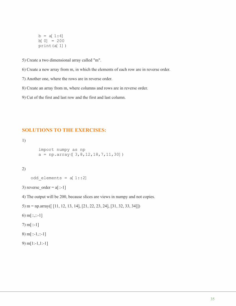
5) Create a two dimensional array called "m".

6) Create a new array from m, in which the elements of each row are in reverse order.

7) Another one, where the rows are in reverse order.

8) Create an array from m, where columns and rows are in reverse order.

9) Cut of the first and last row and the first and last column.

SOLUTIONS TO THE EXERCISES:

1)

import numpy as npa = np.array([3,8,12,18,7,11,30])

2)

odd_elements = a[1::2]

3) reverse_order = a[::-1]

4) The output will be 200, because slices are views in numpy and not copies.

5) m = np.array([ [11, 12, 13, 14], [21, 22, 23, 24], [31, 32, 33, 34]])

6) m[::,::-1]

7) m[::-1]

8) m[::-1,::-1]

9) m[1:-1,1:-1]

35

D A T A T Y P E O B J E C T S , D T Y P E

DTYPE

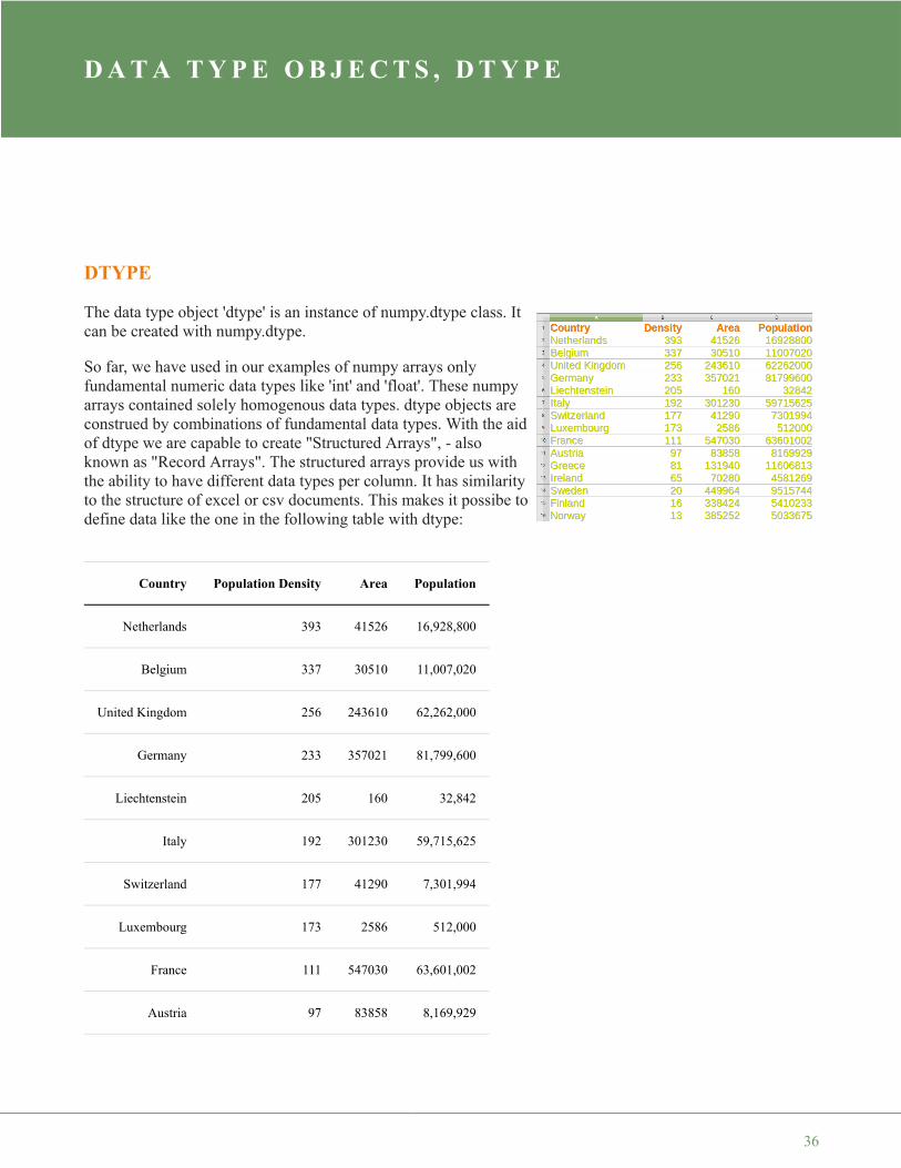
The data type object 'dtype' is an instance of numpy.dtype class. Itcan be created with numpy.dtype.

So far, we have used in our examples of numpy arrays onlyfundamental numeric data types like 'int' and 'float'. These numpyarrays contained solely homogenous data types. dtype objects areconstrued by combinations of fundamental data types. With the aidof dtype we are capable to create "Structured Arrays", - alsoknown as "Record Arrays". The structured arrays provide us withthe ability to have different data types per column. It has similarityto the structure of excel or csv documents. This makes it possibe todefine data like the one in the following table with dtype:

Country Population Density Area Population

Netherlands 393 41526 16,928,800

Belgium 337 30510 11,007,020

United Kingdom 256 243610 62,262,000

Germany 233 357021 81,799,600

Liechtenstein 205 160 32,842

Italy 192 301230 59,715,625

Switzerland 177 41290 7,301,994

Luxembourg 173 2586 512,000

France 111 547030 63,601,002

Austria 97 83858 8,169,929

36

Country Population Density Area Population

Greece 81 131940 11,606,813

Ireland 65 70280 4,581,269

Sweden 20 449964 9,515,744

Finland 16 338424 5,410,233

Norway 13 385252 5,033,675

Before we start with a complex data structure like the previous data, we want to introduce dtype in a verysimple example. We define an int16 data type and call this type i16. (We have to admit, that this is not a nicename, but we use it only here!). The elements of the list 'lst' are turned into i16 types to create the two-dimensional array A.

import numpy as npi16 = np.dtype(np.int16)print(i16)

lst = [ [3.4, 8.7, 9.9],[1.1, -7.8, -0.7],[4.1, 12.3, 4.8] ]

A = np.array(lst, dtype=i16)

print(A)

We introduced a new name for a basic data type in the previous example. This has nothing to do with thestructured arrays, which we mentioned in the introduction of this chapter of our dtype tutorial.

STRUCTURED ARRAYS

ndarrays are homogeneous data objects, i.e. all elements of an array have to be of the same data type. The datatype dytpe on the other hand allows as to define separate data types for each column.

int16[[ 3 8 9][ 1 -7 0][ 4 12 4]]

37

Now we will take the first step towards implementing the table with European countries and the informationon population, area and population density. We create a structured array with the 'density' column. The datatype is defined as np.dtype([('density', np.int)]) . We assign this data type to the variable 'dt'for the sake of convenience. We use this data type in the darray definition, in which we use the first threedensities.

import numpy as npdt = np.dtype([('density', np.int32)])

x = np.array([(393,), (337,), (256,)],dtype=dt)

print(x)

print("\nThe internal representation:")print(repr(x))

We can access the content of the density column by indexing x with the key 'density'. It looks like accessing adictionary in Python:

print(x['density'])

You may wonder that we have used 'np.int32' in our definition and the internal representation shows '<i4'. Wecan use in the dtype definition the type directly (e.g. np.int32) or we can use a string (e.g. 'i4'). So, we couldhave defined our dtype like this as well:

dt = np.dtype([('density', 'i4')])x = np.array([(393,), (337,), (256,)],

dtype=dt)print(x)

The 'i' means integer and the 4 means 4 bytes. What about the less-than sign in front of i4 in the result? Wecould have written '<i4' in our definition as well. We can prefix a type with the '<' and '>' sign. '<' means that

[(393,) (337,) (256,)]

The internal representation:array([(393,), (337,), (256,)],

dtype=[('density', '<i4')])

[393 337 256]

[(393,) (337,) (256,)]

38

the encoding will be little-endian and '>' means that the encoding will be big-endian. No prefix means that weget the native byte ordering. We demonstrate this in the following by defining a double-precision floating-point number in various orderings:

# little-endian orderingdt = np.dtype('<d')print(dt.name, dt.byteorder, dt.itemsize)

# big-endian orderingdt = np.dtype('>d')print(dt.name, dt.byteorder, dt.itemsize)

# native byte orderingdt = np.dtype('d')print(dt.name, dt.byteorder, dt.itemsize)

The equal character '=' stands for 'native byte ordering', defined by the operating system. In our case thismeans 'little-endian', because we use a Linux computer.

Another thing in our density array might be confusing. We defined the array with a list containing one-tuples.So you may ask yourself, if it is possible to use tuples and lists interchangeably? This is not possible. Thetuples are used to define the records - in our case consisting solely of a density - and the list is the 'container'for the records or in other words 'the lists are cursed upon'. The tuples define the atomic elements of thestructure and the lists the dimensions.

Now we will add the country name, the area and the population number to our data type:

dt = np.dtype([('country', 'S20'), ('density', 'i4'), ('area', 'i4'), ('population', 'i4')])population_table = np.array([

('Netherlands', 393, 41526, 16928800),('Belgium', 337, 30510, 11007020),('United Kingdom', 256, 243610, 62262000),('Germany', 233, 357021, 81799600),('Liechtenstein', 205, 160, 32842),('Italy', 192, 301230, 59715625),('Switzerland', 177, 41290, 7301994),('Luxembourg', 173, 2586, 512000),('France', 111, 547030, 63601002),('Austria', 97, 83858, 8169929),('Greece', 81, 131940, 11606813),

float64 = 8float64 > 8float64 = 8

39

('Ireland', 65, 70280, 4581269),('Sweden', 20, 449964, 9515744),('Finland', 16, 338424, 5410233),('Norway', 13, 385252, 5033675)],dtype=dt)

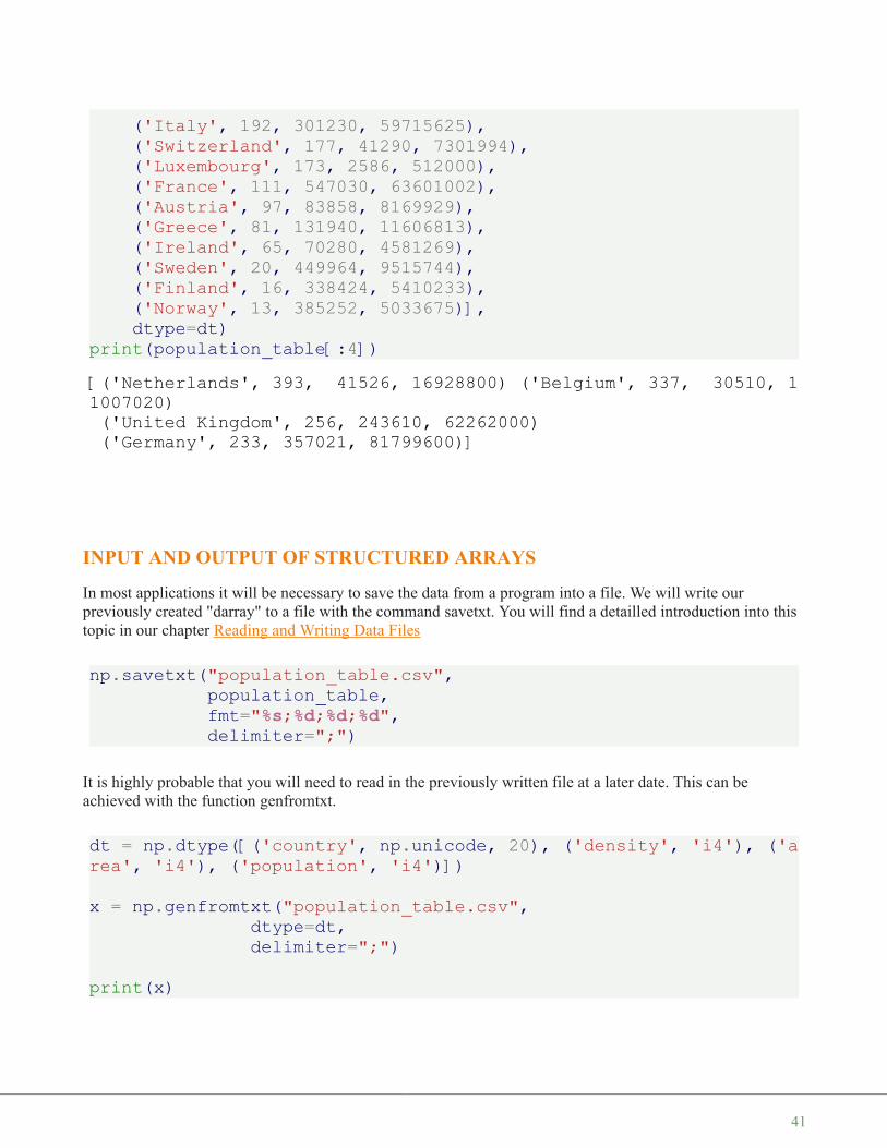
print(population_table[:4])

We can acces every column individually:

print(population_table['density'])print(population_table['country'])print(population_table['area'][2:5])

UNICODE STRINGS IN ARRAY

Some may have noticed that the strings in our previous array have been prefixed with a lower case "b". Thismeans that we have created binary strings with the definition "('country', 'S20')". To get unicode strings weexchange this with the definition "('country', np.unicode, 20)". We will redefine our population table now:

dt = np.dtype([('country', np.unicode, 20),('density', 'i4'),('area', 'i4'),('population', 'i4')])

population_table = np.array([('Netherlands', 393, 41526, 16928800),('Belgium', 337, 30510, 11007020),('United Kingdom', 256, 243610, 62262000),('Germany', 233, 357021, 81799600),('Liechtenstein', 205, 160, 32842),

[(b'Netherlands', 393, 41526, 16928800)(b'Belgium', 337, 30510, 11007020)(b'United Kingdom', 256, 243610, 62262000)(b'Germany', 233, 357021, 81799600)]

[393 337 256 233 205 192 177 173 111 97 81 65 20 16 13][b'Netherlands' b'Belgium' b'United Kingdom' b'Germany' b'Liechtenstein'b'Italy' b'Switzerland' b'Luxembourg' b'France' b'Austria' b'Gree

ce'b'Ireland' b'Sweden' b'Finland' b'Norway']

[243610 357021 160]

40

('Italy', 192, 301230, 59715625),('Switzerland', 177, 41290, 7301994),('Luxembourg', 173, 2586, 512000),('France', 111, 547030, 63601002),('Austria', 97, 83858, 8169929),('Greece', 81, 131940, 11606813),('Ireland', 65, 70280, 4581269),('Sweden', 20, 449964, 9515744),('Finland', 16, 338424, 5410233),('Norway', 13, 385252, 5033675)],dtype=dt)

print(population_table[:4])

INPUT AND OUTPUT OF STRUCTURED ARRAYS

In most applications it will be necessary to save the data from a program into a file. We will write ourpreviously created "darray" to a file with the command savetxt. You will find a detailled introduction into thistopic in our chapter Reading and Writing Data Files

np.savetxt("population_table.csv",population_table,fmt="%s;%d;%d;%d",delimiter=";")

It is highly probable that you will need to read in the previously written file at a later date. This can beachieved with the function genfromtxt.

dt = np.dtype([('country', np.unicode, 20), ('density', 'i4'), ('area', 'i4'), ('population', 'i4')])

x = np.genfromtxt("population_table.csv",dtype=dt,delimiter=";")

print(x)

[('Netherlands', 393, 41526, 16928800) ('Belgium', 337, 30510, 11007020)('United Kingdom', 256, 243610, 62262000)('Germany', 233, 357021, 81799600)]

41

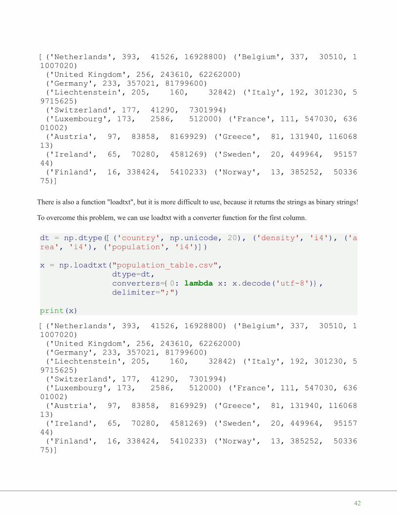
There is also a function "loadtxt", but it is more difficult to use, because it returns the strings as binary strings!

To overcome this problem, we can use loadtxt with a converter function for the first column.

dt = np.dtype([('country', np.unicode, 20), ('density', 'i4'), ('area', 'i4'), ('population', 'i4')])

x = np.loadtxt("population_table.csv",dtype=dt,converters={0: lambda x: x.decode('utf-8')},delimiter=";")

print(x)

[('Netherlands', 393, 41526, 16928800) ('Belgium', 337, 30510, 11007020)('United Kingdom', 256, 243610, 62262000)('Germany', 233, 357021, 81799600)('Liechtenstein', 205, 160, 32842) ('Italy', 192, 301230, 5

9715625)('Switzerland', 177, 41290, 7301994)('Luxembourg', 173, 2586, 512000) ('France', 111, 547030, 636

01002)('Austria', 97, 83858, 8169929) ('Greece', 81, 131940, 116068

13)('Ireland', 65, 70280, 4581269) ('Sweden', 20, 449964, 95157

44)('Finland', 16, 338424, 5410233) ('Norway', 13, 385252, 50336

75)]

[('Netherlands', 393, 41526, 16928800) ('Belgium', 337, 30510, 11007020)('United Kingdom', 256, 243610, 62262000)('Germany', 233, 357021, 81799600)('Liechtenstein', 205, 160, 32842) ('Italy', 192, 301230, 5

9715625)('Switzerland', 177, 41290, 7301994)('Luxembourg', 173, 2586, 512000) ('France', 111, 547030, 636

01002)('Austria', 97, 83858, 8169929) ('Greece', 81, 131940, 116068

13)('Ireland', 65, 70280, 4581269) ('Sweden', 20, 449964, 95157

44)('Finland', 16, 338424, 5410233) ('Norway', 13, 385252, 50336

75)]

42

EXERCISES:

Before you go on, you may take time to do some exercises to deepen the understanding of the previouslylearned stuff.

1. Exercise:Define a structured array with two columns. The first column contains the product ID, which canbe defined as an int32. The second column shall contain the price for the product. How can youprint out the column with the product IDs, the first row and the price for the third article of thisstructured array?

2. Exercise:Figure out a data type definition for time records with entries for hours, minutes and seconds.

SOLUTIONS:

Solution to the first exercise:

import numpy as npmytype = [('productID', np.int32), ('price', np.float64)]

stock = np.array([(34765, 603.76),(45765, 439.93),(99661, 344.19),(12129, 129.39)], dtype=mytype)

print(stock[1])print(stock["productID"])print(stock[2]["price"])print(stock)

Solution to the second exercise:

(45765, 439.93)[34765 45765 99661 12129]344.19[(34765, 603.76) (45765, 439.93) (99661, 344.19) (12129, 129.39)]

43

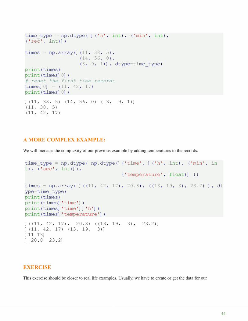
time_type = np.dtype( [('h', int), ('min', int),('sec', int)])

times = np.array([(11, 38, 5),(14, 56, 0),(3, 9, 1)], dtype=time_type)

print(times)print(times[0])# reset the first time record:times[0] = (11, 42, 17)print(times[0])

A MORE COMPLEX EXAMPLE:

We will increase the complexity of our previous example by adding temperatures to the records.

time_type = np.dtype( np.dtype([('time', [('h', int), ('min', int), ('sec', int)]),

('temperature', float)] ))

times = np.array( [((11, 42, 17), 20.8), ((13, 19, 3), 23.2) ], dtype=time_type)print(times)print(times['time'])print(times['time']['h'])print(times['temperature'])

EXERCISE

This exercise should be closer to real life examples. Usually, we have to create or get the data for our

[(11, 38, 5) (14, 56, 0) ( 3, 9, 1)](11, 38, 5)(11, 42, 17)

[((11, 42, 17), 20.8) ((13, 19, 3), 23.2)][(11, 42, 17) (13, 19, 3)][11 13][ 20.8 23.2]

44

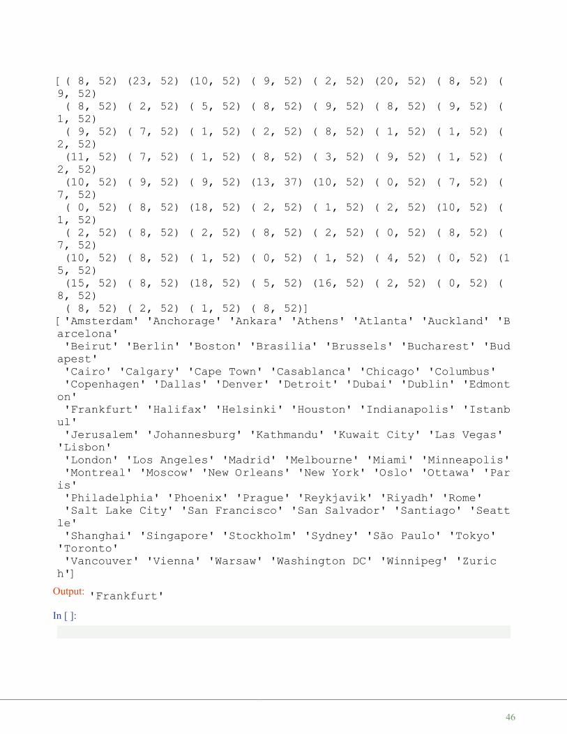
structured array from some data base or file. We will use the list, which we have created in our chapter on fileI/O "File Management". The list has been saved with the aid of pickle.dump in the file cities_and_times.pkl.

So the first task consists in unpickling our data:

import picklefh = open("cities_and_times.pkl", "br")cities_and_times = pickle.load(fh)print(cities_and_times[:30])

Turning our data into a structured array:

time_type = np.dtype([('city', 'U30'), ('day', 'U3'), ('time',[('h', int), ('min', int)])])

times = np.array( cities_and_times , dtype=time_type)print(times['time'])print(times['city'])x = times[27]x[0]

[('Amsterdam', 'Sun', (8, 52)), ('Anchorage', 'Sat', (23, 52)),('Ankara', 'Sun', (10, 52)), ('Athens', 'Sun', (9, 52)), ('Atlanta', 'Sun', (2, 52)), ('Auckland', 'Sun', (20, 52)), ('Barcelona','Sun', (8, 52)), ('Beirut', 'Sun', (9, 52)), ('Berlin', 'Sun',(8, 52)), ('Boston', 'Sun', (2, 52)), ('Brasilia', 'Sun', (5, 52)), ('Brussels', 'Sun', (8, 52)), ('Bucharest', 'Sun', (9, 52)),('Budapest', 'Sun', (8, 52)), ('Cairo', 'Sun', (9, 52)), ('Calgary', 'Sun', (1, 52)), ('Cape Town', 'Sun', (9, 52)), ('Casablanca', 'Sun', (7, 52)), ('Chicago', 'Sun', (1, 52)), ('Columbus', 'Sun', (2, 52)), ('Copenhagen', 'Sun', (8, 52)), ('Dallas', 'Sun',(1, 52)), ('Denver', 'Sun', (1, 52)), ('Detroit', 'Sun', (2, 52)), ('Dubai', 'Sun', (11, 52)), ('Dublin', 'Sun', (7, 52)), ('Edmonton', 'Sun', (1, 52)), ('Frankfurt', 'Sun', (8, 52)), ('Halifax', 'Sun', (3, 52)), ('Helsinki', 'Sun', (9, 52))]

45

In [ ]:

[( 8, 52) (23, 52) (10, 52) ( 9, 52) ( 2, 52) (20, 52) ( 8, 52) (9, 52)( 8, 52) ( 2, 52) ( 5, 52) ( 8, 52) ( 9, 52) ( 8, 52) ( 9, 52) (

1, 52)( 9, 52) ( 7, 52) ( 1, 52) ( 2, 52) ( 8, 52) ( 1, 52) ( 1, 52) (

2, 52)(11, 52) ( 7, 52) ( 1, 52) ( 8, 52) ( 3, 52) ( 9, 52) ( 1, 52) (

2, 52)(10, 52) ( 9, 52) ( 9, 52) (13, 37) (10, 52) ( 0, 52) ( 7, 52) (

7, 52)( 0, 52) ( 8, 52) (18, 52) ( 2, 52) ( 1, 52) ( 2, 52) (10, 52) (

1, 52)( 2, 52) ( 8, 52) ( 2, 52) ( 8, 52) ( 2, 52) ( 0, 52) ( 8, 52) (

7, 52)(10, 52) ( 8, 52) ( 1, 52) ( 0, 52) ( 1, 52) ( 4, 52) ( 0, 52) (1

5, 52)(15, 52) ( 8, 52) (18, 52) ( 5, 52) (16, 52) ( 2, 52) ( 0, 52) (

8, 52)( 8, 52) ( 2, 52) ( 1, 52) ( 8, 52)]

['Amsterdam' 'Anchorage' 'Ankara' 'Athens' 'Atlanta' 'Auckland' 'Barcelona''Beirut' 'Berlin' 'Boston' 'Brasilia' 'Brussels' 'Bucharest' 'Bud

apest''Cairo' 'Calgary' 'Cape Town' 'Casablanca' 'Chicago' 'Columbus''Copenhagen' 'Dallas' 'Denver' 'Detroit' 'Dubai' 'Dublin' 'Edmont

on''Frankfurt' 'Halifax' 'Helsinki' 'Houston' 'Indianapolis' 'Istanb

ul''Jerusalem' 'Johannesburg' 'Kathmandu' 'Kuwait City' 'Las Vegas'

'Lisbon''London' 'Los Angeles' 'Madrid' 'Melbourne' 'Miami' 'Minneapolis''Montreal' 'Moscow' 'New Orleans' 'New York' 'Oslo' 'Ottawa' 'Par

is''Philadelphia' 'Phoenix' 'Prague' 'Reykjavik' 'Riyadh' 'Rome''Salt Lake City' 'San Francisco' 'San Salvador' 'Santiago' 'Seatt

le''Shanghai' 'Singapore' 'Stockholm' 'Sydney' 'São Paulo' 'Tokyo'

'Toronto''Vancouver' 'Vienna' 'Warsaw' 'Washington DC' 'Winnipeg' 'Zuric

h']Output: 'Frankfurt'

46

47

N U M E R I C A L O P E R A T I O N S O N N U M P YA R R A Y S

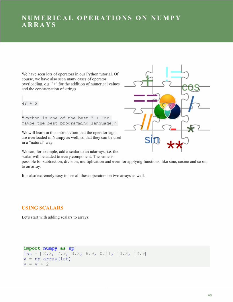
We have seen lots of operators in our Python tutorial. Ofcourse, we have also seen many cases of operatoroverloading, e.g. "+" for the addition of numerical valuesand the concatenation of strings.

42 + 5

"Python is one of the best " + "ormaybe the best programming language!"

We will learn in this introduction that the operator signsare overloaded in Numpy as well, so that they can be usedin a "natural" way.

We can, for example, add a scalar to an ndarrays, i.e. thescalar will be added to every component. The same ispossible for subtraction, division, multiplication and even for applying functions, like sine, cosine and so on,to an array.

It is also extremely easy to use all these operators on two arrays as well.

USING SCALARS

Let's start with adding scalars to arrays:

import numpy as nplst = [2,3, 7.9, 3.3, 6.9, 0.11, 10.3, 12.9]v = np.array(lst)v = v + 2

48

print(v)

Multiplication, Subtraction, Division and exponentiation are as easy as the previous addition:

print(v * 2.2)

print(v - 1.38)

print(v ** 2)print(v ** 1.5)

We started this example with a list lst, which we turned into the array v. Do you know how to perform theabove operations on a list, i.e. multiply, add, subtract and exponentiate every element of the list with a scalar?We could use a for loop for this purpose. Let us do it for the addition without loss of generality. We will addthe value 2 to every element of the list:

lst = [2,3, 7.9, 3.3, 6.9, 0.11, 10.3, 12.9]res = []for val in lst:

res.append(val + 2)

print(res)

Even though this solution works it is not the Pythonic way to do it. We will rather use a list comprehension forthis purpose than the clumsy solution above. If you are not familar with this approach, you may consult ourchapter on list comprehension in our Python course.

res = [ val + 2 for val in lst]print(res)

[ 4. 5. 9.9 5.3 8.9 2.11 12.3 14.9 ]

[ 4.4 6.6 17.38 7.26 15.18 0.242 22.66 28.38 ]

[ 0.62 1.62 6.52 1.92 5.52 -1.27 8.92 11.52]

[ 4.00000000e+00 9.00000000e+00 6.24100000e+01 1.08900000e+01

4.76100000e+01 1.21000000e-02 1.06090000e+02 1.66410000e+02][ 2.82842712e+00 5.19615242e+00 2.22044815e+01 5.99474770e+00

1.81248172e+01 3.64828727e-02 3.30564215e+01 4.63323753e+01]

[4, 5, 9.9, 5.3, 8.9, 2.11, 12.3, 14.9]

49

Even though we had already measured the time consumed by Numpy compared to "plane" Python, we willcompare these two approaches as well:

v = np.random.randint(0, 100, 1000)

%timeit v + 1

lst = list(v)

%timeit [ val + 2 for val in lst]

ARITHMETIC OPERATIONS WITH TWO ARRAYS

If we use another array instead of a scalar, the elements of both arrays will be component-wise combined:

import numpy as npA = np.array([ [11, 12, 13], [21, 22, 23], [31, 32, 33] ])B = np.ones((3,3))

print("Adding to arrays: ")print(A + B)

print("\nMultiplying two arrays: ")print(A * (B + 1))

[4, 5, 9.9, 5.3, 8.9, 2.11, 12.3, 14.9]

1000000 loops, best of 3: 1.69 µs per loop

1000 loops, best of 3: 452 µs per loop

Adding to arrays:[[ 12. 13. 14.][ 22. 23. 24.][ 32. 33. 34.]]

Multiplying two arrays:[[ 22. 24. 26.][ 42. 44. 46.][ 62. 64. 66.]]

50

"A * B" in the previous example shouldn't be mistaken for matrix multiplication. The elements are solelycomponent-wise multiplied.

MATRIX MULTIPLICATION:

For this purpose, we can use the dot product. Using the previous arrays, we can calculate the matrixmultiplication:

np.dot(A, B)

DEFINITION OF THE DOT PRODUCT

The dot product is defined like this:

dot(a, b, out=None)

For 2-D arrays the dot product is equivalent to matrix multiplication. For 1-D arrays it is the same as the innerproduct of vectors (without complex conjugation). For N dimensions it is a sum product over the last axis of 'a'and the second-to-last of 'b'::

Parameter Meaning

a array or array like argument

b array or array like argument

out'out' is an optional parameter, which must have the exact kind of what would be returned, if it was not used. This is a

performance feature. Therefore, if these conditions are not met, an exception is raised, instead of attempting to beflexible.

The function dot returns the dot product of 'a' and 'b'. If 'a' and 'b' are both scalars or both 1-D arrays then ascalar is returned; otherwise an array will returned.

It will raise a ValueError, if the shape of the last dimension of 'a' is not the same size as the shape of the

Output: array([[ 36., 36., 36.],[ 66., 66., 66.],[ 96., 96., 96.]])

51

second-to-last dimension of 'b', i.e. a.shape[-1] == b.shape[-2]

EXAMPLES OF USING THE DOT PRODUCT

We will begin with the cases in which both arguments are scalars or one-dimensional array:

print(np.dot(3, 4))x = np.array([3])y = np.array([4])print(x.ndim)print(np.dot(x, y))

x = np.array([3, -2])y = np.array([-4, 1])print(np.dot(x, y))

Let's go to the two-dimensional use case:

A = np.array([ [1, 2, 3],[3, 2, 1] ])

B = np.array([ [2, 3, 4, -2],[1, -1, 2, 3],[1, 2, 3, 0] ])

# es muss gelten:print(A.shape[-1] == B.shape[-2], A.shape[1])print(np.dot(A, B))

We can learn from the previous example that the number of columns of the first two-dimension array have tobe the same as the number of the lines of the second two-dimensional array.

12112-14

(True, 3)[[ 7 7 17 4][ 9 9 19 0]]

52

THE DOT PRODUCT IN THE 3-DIMENSIONAL CASE

It's getting really vexing, if we use 3-dimensional arrays as the arguments of dot.

We will use two symmetrical three-dimensional arrays in the first example:

import numpy as npX = np.array( [[[3, 1, 2],

[4, 2, 2],[2, 4, 1]],

[[3, 2, 2],[4, 4, 3],[4, 1, 1]],

[[2, 2, 1],[3, 1, 3],[3, 2, 3]]])

Y = np.array( [[[2, 3, 1],[2, 2, 4],[3, 4, 4]],

[[1, 4, 1],[4, 1, 2],[4, 1, 2]],

[[1, 2, 3],[4, 1, 1],[3, 1, 4]]])

R = np.dot(X, Y)

print("The shapes:")print(X.shape)print(Y.shape)print(R.shape)

print("\nThe Result R:")print(R)

53

To demonstrate how the dot product in the three-dimensional case works, we will use different arrays with

The shapes:(3, 3, 3)(3, 3, 3)(3, 3, 3, 3)

The Result R:[[[[14 19 15]

[15 15 9][13 9 18]]

[[18 24 20][20 20 12][18 12 22]]

[[15 18 22][22 13 12][21 9 14]]]

[[[16 21 19][19 16 11][17 10 19]]

[[25 32 32][32 23 18][29 15 28]]

[[13 18 12][12 18 8][11 10 17]]]

[[[11 14 14][14 11 8][13 7 12]]

[[17 23 19][19 16 11][16 10 22]]

[[19 25 23][23 17 13][20 11 23]]]]

54

non-symmetrical shapes in the following example:

import numpy as npX = np.array(

[[[3, 1, 2],[4, 2, 2]],

[[-1, 0, 1],[1, -1, -2]],

[[3, 2, 2],[4, 4, 3]],

[[2, 2, 1],[3, 1, 3]]])

Y = np.array([[[2, 3, 1, 2, 1],

[2, 2, 2, 0, 0],[3, 4, 0, 1, -1]],

[[1, 4, 3, 2, 2],[4, 1, 1, 4, -3],[4, 1, 0, 3, 0]]])

R = np.dot(X, Y)

print("X.shape: ", X.shape, " X.ndim: ", X.ndim)print("Y.shape: ", Y.shape, " Y.ndim: ", Y.ndim)print("R.shape: ", R.shape, "R.ndim: ", R.ndim)

print("\nThe result array R:\n")print(R)

55

Let's have a look at the following sum products:

i = 0for j in range(X.shape[1]):

for k in range(Y.shape[0]):for m in range(Y.shape[2]):

fmt = " sum(X[{}, {}, :] * Y[{}, :, {}] : {}"arguments = (i, j, k, m, sum(X[i, j, :] * Y[k, :, m]))print(fmt.format(*arguments))

('X.shape: ', (4, 2, 3), ' X.ndim: ', 3)('Y.shape: ', (2, 3, 5), ' Y.ndim: ', 3)('R.shape: ', (4, 2, 2, 5), 'R.ndim: ', 4)

The result array R:

[[[[ 14 19 5 8 1][ 15 15 10 16 3]]

[[ 18 24 8 10 2][ 20 20 14 22 2]]]

[[[ 1 1 -1 -1 -2][ 3 -3 -3 1 -2]]

[[ -6 -7 -1 0 3][-11 1 2 -8 5]]]

[[[ 16 21 7 8 1][ 19 16 11 20 0]]

[[ 25 32 12 11 1][ 32 23 16 33 -4]]]

[[[ 11 14 6 5 1][ 14 11 8 15 -2]]

[[ 17 23 5 9 0][ 19 16 10 19 3]]]]

56

Hopefully, you have noticed that we have created the elements of R[0], one ofter the other.

print(R[0])

This means that we could have created the array R by applying the sum products in the way above. To "prove"this, we will create an array R2 by using the sum product, which is equal to R in the following example:

R2 = np.zeros(R.shape, dtype=np.int)

for i in range(X.shape[0]):for j in range(X.shape[1]):

for k in range(Y.shape[0]):for m in range(Y.shape[2]):

R2[i, j, k, m] = sum(X[i, j, :] * Y[k, :, m])

print( np.array_equal(R, R2) )

sum(X[0, 0, :] * Y[0, :, 0] : 14sum(X[0, 0, :] * Y[0, :, 1] : 19sum(X[0, 0, :] * Y[0, :, 2] : 5sum(X[0, 0, :] * Y[0, :, 3] : 8sum(X[0, 0, :] * Y[0, :, 4] : 1sum(X[0, 0, :] * Y[1, :, 0] : 15sum(X[0, 0, :] * Y[1, :, 1] : 15sum(X[0, 0, :] * Y[1, :, 2] : 10sum(X[0, 0, :] * Y[1, :, 3] : 16sum(X[0, 0, :] * Y[1, :, 4] : 3sum(X[0, 1, :] * Y[0, :, 0] : 18sum(X[0, 1, :] * Y[0, :, 1] : 24sum(X[0, 1, :] * Y[0, :, 2] : 8sum(X[0, 1, :] * Y[0, :, 3] : 10sum(X[0, 1, :] * Y[0, :, 4] : 2sum(X[0, 1, :] * Y[1, :, 0] : 20sum(X[0, 1, :] * Y[1, :, 1] : 20sum(X[0, 1, :] * Y[1, :, 2] : 14sum(X[0, 1, :] * Y[1, :, 3] : 22sum(X[0, 1, :] * Y[1, :, 4] : 2

[[[14 19 5 8 1][15 15 10 16 3]]

[[18 24 8 10 2][20 20 14 22 2]]]

57

MATRICES VS. TWO-DIMENSIONAL ARRAYS

Some may have taken two-dimensional arrays of Numpy as matrices. This is principially all right, becausethey behave in most aspects like our mathematical idea of a matrix. We even saw that we can perform matrixmultiplication on them. Yet, there is a subtle difference. There are "real" matrices in Numpy. They are a subsetof the two-dimensional arrays. We can turn a two-dimensional array into a matrix by applying the "mat"function. The main difference shows, if you multiply two two-dimensional arrays or two matrices. We get realmatrix multiplication by multiplying two matrices, but the two-dimensional arrays will be only multipliedcomponent-wise:

import numpy as npA = np.array([ [1, 2, 3], [2, 2, 2], [3, 3, 3] ])B = np.array([ [3, 2, 1], [1, 2, 3], [-1, -2, -3] ])

R = A * Bprint(R)

MA = np.mat(A)MB = np.mat(B)

R = MA * MBprint(R)

COMPARISON OPERATORS

We are used to comparison operators from Python, when we apply them to integers, floats or strings forexample. We use them to test for True or False. If we compare two arrays, we don't get a simple True or Falseas a return value. The comparisons are performed elementswise. This means that we get a Boolean array as a

True

[[ 3 4 3][ 2 4 6][-3 -6 -9]]

[[ 2 0 -2][ 6 4 2][ 9 6 3]]

58

return value:

import numpy as npA = np.array([ [11, 12, 13], [21, 22, 23], [31, 32, 33] ])B = np.array([ [11, 102, 13], [201, 22, 203], [31, 32, 303] ])

A == B

It is possible to compare complete arrays for equality as well. We use array_equal for this purpose.array_equal returns True if two arrays have the same shape and elements, otherwise False will be returned.

print(np.array_equal(A, B))print(np.array_equal(A, A))

LOGICAL OPERATORS

We can also apply the logical 'or' and the logical 'and' to arrays elementwise. We can use the functions'logical_or' and 'logical_and' to this purpose.

a = np.array([ [True, True], [False, False]])b = np.array([ [True, False], [True, False]])print(np.logical_or(a, b))print(np.logical_and(a, b))

Output: array([[ True, False, True],[False, True, False],[ True, True, False]], dtype=bool)

FalseTrue

[[ True True][ True False]]

[[ True False][False False]]

59

APPLYING OPERATORS ON ARRAYS WITH DIFFERENT SHAPES

So far we have covered two different cases with basic operators like "+" or "*":

• an operator applied to an array and a scalar• an operator applied to two arrays of the same shape

We will see in the following that we can also apply operators on arrays, if they have different shapes. Yet, itworks only under certain conditions.

BROADCASTING

Numpy provides a powerful mechanism, called Broadcasting, which allows to perform arithmetic operationson arrays of different shapes. This means that we have a smaller array and a larger array, and we transform orapply the smaller array multiple times to perform some operation on the larger array. In other words: Undercertain conditions, the smaller array is "broadcasted" in a way that it has the same shape as the larger array.

With the aid of broadcasting we can avoid loops in our Python program. The looping occurs implicitly in theNumpy implementations, i.e. in C. We also avoid creating unnecessary copies of our data.

We demonstrate the operating principle of broadcasting in three simple and descriptive examples.

FIRST EXAMPLE OF BROADCASTING:import numpy as npA = np.array([ [11, 12, 13], [21, 22, 23], [31, 32, 33] ])B = np.array([1, 2, 3])

print("Multiplication with broadcasting: ")print(A * B)print("... and now addition with broadcasting: ")print(A + B)

60

The following diagram illustrates the way of working of broadcasting:

B is treated as if it were construed like this:

B = np.array([[1, 2, 3],] * 3)print(B)

SECOND EXAMPLE:

For this example, we need to know how to turn a row vector into a column vector:

B = np.array([1, 2, 3])B[:, np.newaxis]

Multiplication with broadcasting:[[11 24 39][21 44 69][31 64 99]]

... and now addition with broadcasting:[[12 14 16][22 24 26][32 34 36]]

[[1 2 3][1 2 3][1 2 3]]

61

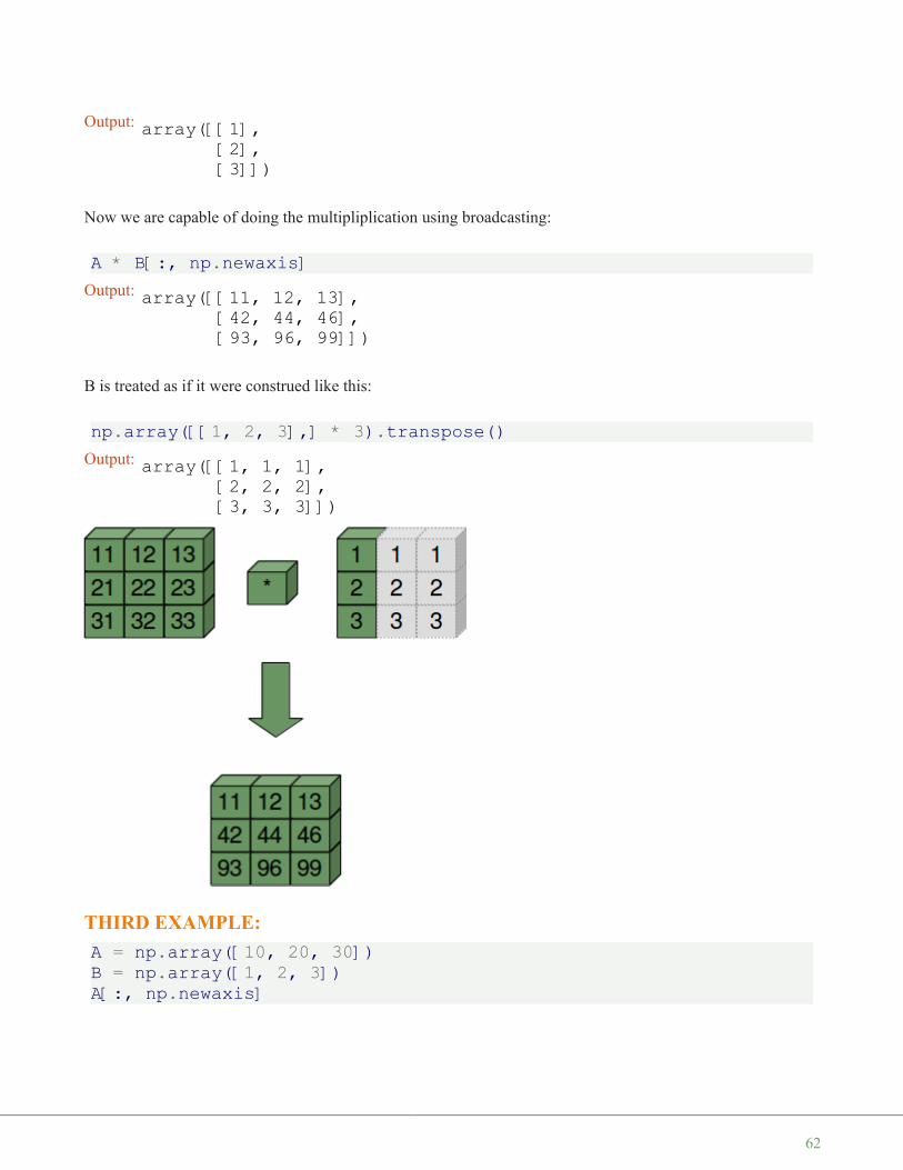
Now we are capable of doing the multipliplication using broadcasting:

A * B[:, np.newaxis]

B is treated as if it were construed like this:

np.array([[1, 2, 3],] * 3).transpose()

THIRD EXAMPLE:A = np.array([10, 20, 30])B = np.array([1, 2, 3])A[:, np.newaxis]

Output: array([[1],[2],[3]])

Output: array([[11, 12, 13],[42, 44, 46],[93, 96, 99]])

Output: array([[1, 1, 1],[2, 2, 2],[3, 3, 3]])

62

A[:, np.newaxis] * B

ANOTHER WAY TO DO IT

Doing it without broadcasting:

import numpy as npA = np.array([ [11, 12, 13], [21, 22, 23], [31, 32, 33] ])

B = np.array([1, 2, 3])

B = B[np.newaxis, :]B = np.concatenate((B, B, B))

print("Multiplication: ")print(A * B)print("... and now addition again: ")print(A + B)

Output: array([[10],[20],[30]])

Output: array([[10, 20, 30],[20, 40, 60],[30, 60, 90]])

63

Using 'tile':

import numpy as npA = np.array([ [11, 12, 13], [21, 22, 23], [31, 32, 33] ])

B = np.tile(np.array([1, 2, 3]), (3, 1))

print(B)

print("Multiplication: ")print(A * B)print("... and now addition again: ")print(A + B)

DISTANCE MATRIX

In mathematics, computer science and especially graph theory, a distance matrix is a matrix or a two-dimensional array, which contains the distances between the elements of a set, pairwise taken. The size of thistwo-dimensional array in n x n, if the set consists of n elements.

Multiplication:[[11 24 39][21 44 69][31 64 99]]

... and now addition again:[[12 14 16][22 24 26][32 34 36]]

[[1 2 3][1 2 3][1 2 3]]

Multiplication:[[11 24 39][21 44 69][31 64 99]]

... and now addition again:[[12 14 16][22 24 26][32 34 36]]

64

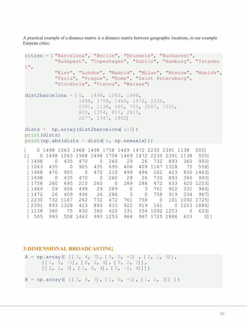
A practical example of a distance matrix is a distance matrix between geographic locations, in our exampleEurpean cities:

cities = ["Barcelona", "Berlin", "Brussels", "Bucharest","Budapest", "Copenhagen", "Dublin", "Hamburg", "Istanbu

l","Kiev", "London", "Madrid", "Milan", "Moscow", "Munich","Paris", "Prague", "Rome", "Saint Petersburg","Stockholm", "Vienna", "Warsaw"]

dist2barcelona = [0, 1498, 1063, 1968,1498, 1758, 1469, 1472, 2230,2391, 1138, 505, 725, 3007, 1055,833, 1354, 857, 2813,2277, 1347, 1862]

dists = np.array(dist2barcelona[:12])print(dists)print(np.abs(dists - dists[:, np.newaxis]))

3-DIMENSIONAL BROADCASTINGA = np.array([ [[3, 4, 7], [5, 0, -1] , [2, 1, 5]],

[[1, 0, -1], [8, 2, 4], [5, 2, 1]],[[2, 1, 3], [1, 9, 4], [5, -2, 4]]])

B = np.array([ [[3, 4, 7], [1, 0, -1], [1, 2, 3]] ])

[ 0 1498 1063 1968 1498 1758 1469 1472 2230 2391 1138 505][[ 0 1498 1063 1968 1498 1758 1469 1472 2230 2391 1138 505][1498 0 435 470 0 260 29 26 732 893 360 993][1063 435 0 905 435 695 406 409 1167 1328 75 558][1968 470 905 0 470 210 499 496 262 423 830 1463][1498 0 435 470 0 260 29 26 732 893 360 993][1758 260 695 210 260 0 289 286 472 633 620 1253][1469 29 406 499 29 289 0 3 761 922 331 964][1472 26 409 496 26 286 3 0 758 919 334 967][2230 732 1167 262 732 472 761 758 0 161 1092 1725][2391 893 1328 423 893 633 922 919 161 0 1253 1886][1138 360 75 830 360 620 331 334 1092 1253 0 633][ 505 993 558 1463 993 1253 964 967 1725 1886 633 0]]

65

B * A

We will use the following transformations in our chapter on Images Manipulation and Processing:

B = np.array([1, 2, 3])

B = B[np.newaxis, :]print(B.shape)B = np.concatenate((B, B, B)).transpose()print(B.shape)B = B[:, np.newaxis]print(B.shape)print(B)

print(A * B)

Output: array([[[ 9, 16, 49],[ 5, 0, 1],[ 2, 2, 15]],

[[ 3, 0, -7],[ 8, 0, -4],[ 5, 4, 3]],

[[ 6, 4, 21],[ 1, 0, -4],[ 5, -4, 12]]])

66

(1, 3)(3, 3)(3, 1, 3)[[[1 1 1]]

[[2 2 2]]

[[3 3 3]]][[[ 3 4 7]

[ 5 0 -1][ 2 1 5]]

[[ 2 0 -2][16 4 8][10 4 2]]

[[ 6 3 9][ 3 27 12][15 -6 12]]]

67

N U M P Y A R R A Y S : C O N C A T E N A T I N G ,F L A T T E N I N G A N D A D D I N G D I M E N S I O N S

So far, we have learned in our tutorial how to createarrays and how to apply numerical operations onnumpy arrays. If we program with numpy, we willcome sooner or later to the point, where we will needfunctions to manipulate the shape or dimension ofarrays. We wil also learn how to concatenate arrays.Furthermore, we will demonstrate the possibilities toadd dimensions to existing arrays and how to stackmultiple arrays. We will end this chapter by showingan easy way to construct new arrays by repeatingexisting arrays.

The picture shows a tesseract. A tesseract is a

hypercube in ℜ4. The tesseract is to the cube as thecube is to the square: the surface of the cube consistsof six square sides, whereas the hypersurface of thetesseract consists of eight cubical cells.

FLATTEN AND RESHAPE ARRAYS

There are two methods to flatten a multidimensional array:

• flatten()• ravel()

FLATTEN

flatten is a ndarry method with an optional keyword parameter "order". order can have the values "C", "F" and"A". The default of order is "C". "C" means to flatten C style in row-major ordering, i.e. the rightmost index"changes the fastest" or in other words: In row-major order, the row index varies the slowest, and the columnindex the quickest, so that a[0,1] follows [0,0]."F" stands for Fortran column-major ordering. "A" means preserve the the C/Fortran ordering.

import numpy as npA = np.array([[[ 0, 1],

[ 2, 3],

68

[ 4, 5],[ 6, 7]],

[[ 8, 9],[10, 11],[12, 13],[14, 15]],

[[16, 17],[18, 19],[20, 21],[22, 23]]])

Flattened_X = A.flatten()print(Flattened_X)

print(A.flatten(order="C"))print(A.flatten(order="F"))print(A.flatten(order="A"))

RAVEL

The order of the elements in the array returned by ravel() is normally "C-style".

ravel(a, order='C')

ravel returns a flattened one-dimensional array. A copy is made only if needed.

The optional keyword parameter "order" can be 'C','F', 'A', or 'K'

'C': C-like order, with the last axis index changing fastest, back to the first axis index changing slowest. "C" isthe default!

'F': Fortran-like index order with the first index changing fastest, and the last index changing slowest.

'A': Fortran-like index order if the array "a" is Fortran contiguous in memory, C-like order otherwise.

'K': read the elements in the order they occur in memory, except for reversing the data when strides arenegative.

[ 0 1 2 3 4 5 6 7 8 9 10 11 12 13 14 15 16 17 18 19 20 21 22 23][ 0 1 2 3 4 5 6 7 8 9 10 11 12 13 14 15 16 17 18 19 20 21 22 23][ 0 8 16 2 10 18 4 12 20 6 14 22 1 9 17 3 11 19 5 13 217 15 23][ 0 1 2 3 4 5 6 7 8 9 10 11 12 13 14 15 16 17 18 19 20 21 22 23]

69

print(A.ravel())

print(A.ravel(order="A"))

print(A.ravel(order="F"))

print(A.ravel(order="A"))

print(A.ravel(order="K"))

RESHAPE

The method reshape() gives a new shape to an array without changing its data, i.e. it returns a new array with anew shape.

reshape(a, newshape, order='C')

Parameter Meaning

a array_like, Array to be reshaped.

newshape int or tuple of ints

order 'C', 'F', 'A', like in flatten or ravel

X = np.array(range(24))Y = X.reshape((3,4,2))Y

[ 0 1 2 3 4 5 6 7 8 9 10 11 12 13 14 15 16 17 18 19 20 21 22 23][ 0 1 2 3 4 5 6 7 8 9 10 11 12 13 14 15 16 17 18 19 20 21 22 23][ 0 8 16 2 10 18 4 12 20 6 14 22 1 9 17 3 11 19 5 13 217 15 23][ 0 1 2 3 4 5 6 7 8 9 10 11 12 13 14 15 16 17 18 19 20 21 22 23][ 0 1 2 3 4 5 6 7 8 9 10 11 12 13 14 15 16 17 18 19 20 21 22 23]

70

CONCATENATING ARRAYS

In the following example we concatenate three one-dimensional arrays to one array. The elements of thesecond array are appended to the first array. After this the elements of the third array are appended:

x = np.array([11,22])y = np.array([18,7,6])z = np.array([1,3,5])c = np.concatenate((x,y,z))print(c)

If we are concatenating multidimensional arrays, we can concatenate the arrays according to axis. Arrays musthave the same shape to be concatenated with concatenate(). In the case of multidimensional arrays, we canarrange them according to the axis. The default value is axis = 0:

x = np.array(range(24))x = x.reshape((3,4,2))y = np.array(range(100,124))y = y.reshape((3,4,2))z = np.concatenate((x,y))print(z)

Output: array([[[ 0, 1],[ 2, 3],[ 4, 5],[ 6, 7]],

[[ 8, 9],[10, 11],[12, 13],[14, 15]],

[[16, 17],[18, 19],[20, 21],[22, 23]]])

[11 22 18 7 6 1 3 5]

71

We do the same concatenation now with axis=1:

z = np.concatenate((x,y),axis = 1)print(z)

[[[ 0 1][ 2 3][ 4 5][ 6 7]]

[[ 8 9][ 10 11][ 12 13][ 14 15]]

[[ 16 17][ 18 19][ 20 21][ 22 23]]

[[100 101][102 103][104 105][106 107]]

[[108 109][110 111][112 113][114 115]]

[[116 117][118 119][120 121][122 123]]]

72

ADDING NEW DIMENSIONS

New dimensions can be added to an array by using slicing and np.newaxis. We illustrate this technique with anexample:

x = np.array([2,5,18,14,4])y = x[:, np.newaxis]print(y)

[[[ 0 1][ 2 3][ 4 5][ 6 7][100 101][102 103][104 105][106 107]]

[[ 8 9][ 10 11][ 12 13][ 14 15][108 109][110 111][112 113][114 115]]

[[ 16 17][ 18 19][ 20 21][ 22 23][116 117][118 119][120 121][122 123]]]

[[ 2][ 5][18][14][ 4]]

73

VECTOR STACKINGA = np.array([3, 4, 5])B = np.array([1,9,0])

print(np.row_stack((A, B)))

print(np.column_stack((A, B)))np.shape(A)

A = np.array([[3, 4, 5],[1, 9, 0],[4, 6, 8]])

np.column_stack((A, A, A))

np.column_stack((A[0], A[0], A[0]))

np.dstack((A, A, A))

[[3 4 5][1 9 0]]

[[3 1][4 9][5 0]]

Output: (3,)

Output: array([[3, 4, 5, 3, 4, 5, 3, 4, 5],[1, 9, 0, 1, 9, 0, 1, 9, 0],[4, 6, 8, 4, 6, 8, 4, 6, 8]])

Output: array([[3, 3, 3],[4, 4, 4],[5, 5, 5]])

74

REPEATING PATTERNS, THE "TILE" METHOD

Sometimes, you want to or have to create a new matrix by repeating an existing matrix multiple times to createa new matrix with a different shape or even dimension. You may have for example a one-dimensional arrayarray([ 3.4]) and you want to turn it into an array array([ 3.4, 3.4, 3.4, 3.4,3.4])

In another usecase you may have a two-dimensional array like np.array([ [1, 2], [3, 4]]) ,which you intend to use as a building block to construe the array with the shape (6, 8):

array([[1, 2, 1, 2, 1, 2, 1, 2],[3, 4, 3, 4, 3, 4, 3, 4],[1, 2, 1, 2, 1, 2, 1, 2],[3, 4, 3, 4, 3, 4, 3, 4],[1, 2, 1, 2, 1, 2, 1, 2],[3, 4, 3, 4, 3, 4, 3, 4]])

The idea of construction is depicted in the following diagram:

Output: array([[[3, 3, 3],[4, 4, 4],[5, 5, 5]],

[[1, 1, 1],[9, 9, 9],[0, 0, 0]],

[[4, 4, 4],[6, 6, 6],[8, 8, 8]]])

75

If this reminds you of tiling a bathroom or a kitchen, you are on the right track: The function which Numpyprovides for this task is called "tile".

The formal syntax of tile looks like this:

tile(A, reps)

An array is constructed by repeating A the number of times given by reps.

'reps' is usually a tuple (or list) which defines the number of repetitions along the corresponding axis /directions. if we set reps to (3, 4) for example, A will be repeated 3 times for the "rows" and 4 times in thedirection of the columna. We demonstrate this in the following example:

import numpy as npx = np.array([ [1, 2], [3, 4]])np.tile(x, (3,4))

import numpy as npx = np.array([ 3.4])

y = np.tile(x, (5,))

print(y)

Output: array([[1, 2, 1, 2, 1, 2, 1, 2],[3, 4, 3, 4, 3, 4, 3, 4],[1, 2, 1, 2, 1, 2, 1, 2],[3, 4, 3, 4, 3, 4, 3, 4],[1, 2, 1, 2, 1, 2, 1, 2],[3, 4, 3, 4, 3, 4, 3, 4]])

76

In the previous tile example, we could have written y = np.tile(x, 5) as well.

If we stick to writing reps in the tuple or list form, or consider reps = 5 as an abbreviation for reps =(5,) , the following is true:

If 'reps' has length n, the dimension of the resulting array will be the maximum of n and A.ndim.

If 'A.ndim < n, 'A' is promoted to be n-dimensional by prepending new axes. So a shape (5,) array is promotedto (1, 5) for 2-D replication, or shape (1, 1, 5) for 3-D replication. If this is not the desired behavior, promote'A' to n-dimensions manually before calling this function.

If 'A.ndim > d', 'reps' is promoted to 'A'.ndim by pre-pending 1's to it.

Thus for an array 'A' of shape (2, 3, 4, 5), a 'reps' of (2, 2) is treated as (1, 1, 2, 2).

Further examples:

import numpy as npx = np.array([[1, 2], [3, 4]])print(np.tile(x, 2))

import numpy as npx = np.array([[1, 2], [3, 4]])print(np.tile(x, (2, 1)))

import numpy as npx = np.array([[1, 2], [3, 4]])print(np.tile(x, (2, 2)))

[ 3.4 3.4 3.4 3.4 3.4]

[[1 2 1 2][3 4 3 4]]

[[1 2][3 4][1 2][3 4]]

[[1 2 1 2][3 4 3 4][1 2 1 2][3 4 3 4]]

77

78

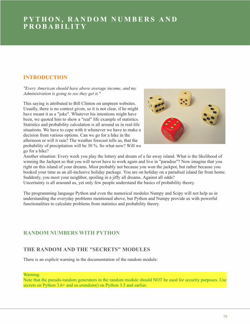
P Y T H O N , R A N D O M N U M B E R S A N DP R O B A B I L I T Y

INTRODUCTION

"Every American should have above average income, and myAdministration is going to see they get it."

This saying is attributed to Bill Clinton on umpteen websites.Usually, there is no context given, so it is not clear, if he mighthave meant it as a "joke". Whatever his intentions might havebeen, we quoted him to show a "real" life example of statistics.Statistics and probability calculation is all around us in real-lifesituations. We have to cope with it whenever we have to make adecision from various options. Can we go for a hike in theafternoon or will it rain? The weather forecast tells us, that theprobability of precipitation will be 30 %. So what now? Will wego for a hike?Another situation: Every week you play the lottery and dream of a far away island. What is the likelihood ofwinning the Jackpot so that you will never have to work again and live in "paradise"? Now imagine that youright on this island of your dreams. Most probably not because you won the jackpot, but rather because youbooked your time as an all-inclusive holiday package. You are on holiday on a paradisal island far from home.Suddenly, you meet your neighbor, spoiling in a jiffy all dreams. Against all odds?Uncertainty is all araound us, yet only few people understand the basics of probability theory.

The programming language Python and even the numerical modules Numpy and Scipy will not help us inunderstanding the everyday problems mentioned above, but Python and Numpy provide us with powerfulfunctionalities to calculate problems from statistics and probability theory.

RANDOM NUMBERS WITH PYTHON

THE RANDOM AND THE "SECRETS" MODULES

There is an explicit warning in the documentation of the random module:

Warning:Note that the pseudo-random generators in the random module should NOT be used for security purposes. Usesecrets on Python 3.6+ and os.urandom() on Python 3.5 and earlier.

79

The default pseudo-random number generator of the random module was designed with the focus onmodelling and simulation, not on security. So, you shouldn't generate sensitive information such as passwords,secure tokens, session keys and similar things by using random. When we say that you shouldn't use therandom module, we mean the basic functionalities "randint", "random", "choise" , and the likes. There is oneexception as you will learn in the next paragraph: SystemRandom

The SystemRandom class offers a suitable way to overcome this security problem. The methods of this classuse an alternate random number generator, which uses tools provided by the operating system (such as /dev/urandom on Unix or CryptGenRandom on Windows.

As there has been great concern that Python developers might inadvertently make serious security errors, -even though the warning is included in the documentaiton, - Python 3.6 comes with a new module "secrets"with a CSPRNG (Cryptographically Strong Pseudo Random Number Generator).

Let's start with creating random float numbers with the random function of the random module. Pleaseremember that it shouldn't be used to generate sensitive information:

import randomrandom_number = random.random()print(random_number)

We will show an alternative and secure approach in the following example, in which we will use the classSystemRandom of the random module. It will use a different random number generator. It uses sources whichare provided by the operating system. This will be /dev/urandom on Unix and CryptGenRandom on windows.The random method of the SystemRandom class generates a float number in the range from 0.0 (included) to1.0 (not included):

from random import SystemRandomcrypto = SystemRandom()print(crypto.random())

GENERATE A LIST OF RANDOM NUMBERS

Quite often you will need more than one random number. We can create a list of random numbers byrepeatedly calling random().

import randomdef random_list(n, secure=True):

random_floats = []if secure:

crypto = random.SystemRandom()

0.34330263184538523

0.8875057137654113

80

random_float = crypto.randomelse:

random_float = random.randomfor _ in range(n):

random_floats.append(random_float())return random_floats

print(random_list(10, secure=False))

The "simple" random function of the random module is a lot faster as we can see in the following:

%%timeitrandom_list(100)

%%timeitrandom_list(100, secure=False)

crypto = random.SystemRandom()[crypto.random() for _ in range(10)]

Alternatively, you can use a list comprehension to create a list of random float numbers:

%%timeit[crypto.random() for _ in range(100)]

[0.9702685982962019, 0.5095131905323179, 0.9324278634720967, 0.9750405405778308, 0.9750927470224396, 0.2383439553695087, 0.03591694433088444, 0.9203791901577599, 0.07793301506800698, 0.46915245764066404]

10000 loops, best of 3: 158 µs per loop

100000 loops, best of 3: 8.64 µs per loop

Output: [0.5832874631978111,0.7494815897496974,0.6982338101218046,0.5164288598133177,0.15423895558995826,0.9447842390510461,0.08095707071826808,0.5407159221282145,0.6124979567571185,0.15764744205801628]

10000 loops, best of 3: 157 µs per loop

81

The fastest and most efficient way will be using the random package of the numpy module:

import numpy as npnp.random.random(10)

%%timeitnp.random.random(100)

Warning:The random package of the Numpy module apparantly - even though it doesn't say so in the documentation -is completely deterministic, using also the Mersenne twister sequence!

RANDOM NUMBERS SATISFYING SUM-TO-ONE CONDITION

It's very easy to create a list of random numbers satisfying the condition that they sum up to one. This way, weturn them into values, which could be used as probalities. We can use any of the methods explained above tonormalize a list of random values. All we have to do is divide every value by the sum of the values. Theeasiest way will be using numpy again of course:

import numpy as nplist_of_random_floats = np.random.random(100)sum_of_values = list_of_random_floats.sum()print(sum_of_values)normalized_values = list_of_random_floats / sum_of_valuesprint(normalized_values.sum())

Output: array([ 0.0422172 , 0.98285327, 0.40386413, 0.34629582,0.25666744,

0.69242112, 0.9231164 , 0.47445382, 0.63654389,0.06781786])

The slowest run took 16.56 times longer than the fastest. This could mean that an intermediate result is being cached.100000 loops, best of 3: 2.1 µs per loop

52.35098391371.0

82

GENERATING RANDOM STRINGS OR PASSWORDS WITH PYTHON

We assume that you don't use and don't like weak passwords like "123456", "password", "qwerty" and thelikes. Believe it or not, these passwords are always ranking to 10. So you looking for a safe password? Youwant to create passwords with Python? But don't use some of the functions ranking top 10 in the searchresults, because you may use a functions using the random function of the random module.

We will define a strong random password generator, which uses the SystemRandom class. This class uses, aswe have alreay mentioned, a cryptographically strong pseudo random number generator:

from random import SystemRandomsr = SystemRandom() # create an instance of the SystemRandom class

def generate_password(length,valid_chars=None):

""" generate_password(length, check_char) -> passwordlength: the length of the created passwordcheck_char: a Boolean function used to check the validity

of a char"""if valid_chars==None:

valid_chars = "ABCDEFGHIJKLMNOPQRSTUVWXYZ"valid_chars += valid_chars.lower() + "0123456789"

password = ""counter = 0while counter < length:

rnum = sr.randint(0, 128)char = chr(rnum)if char in valid_chars:

password += chr(rnum)counter += 1

return password

print("Automatically generated password by Python: " + generate_password(15))Automatically generated password by Python: ll6Zki280gfUqMD

83

RANDOM INTEGER NUMBERS

Everybody is familar with creating random integer numbers without computers. If you roll a die, you create arandom number between 1 and 6. In terms of probability theory, we would call "the rolling of the die" anexperiment with a result from the set of possible outcomes {1, 2, 3, 4, 5, 6}. It is also called the sample spaceof the experiment.

How can we simulate the rolling of a die in Python? We don't need Numpy for this aim. "Pure" Python and itsrandom module is enough.

import randomoutcome = random.randint(1,6)print(outcome)

Let's roll our virtual die 10 times:

import random[ random.randint(1, 6) for _ in range(10) ]

We can accomplish this easier with the NumPy package random:

import numpy as npoutcome = np.random.randint(1, 7, size=10)print(outcome)

You may have noticed, that we used 7 instead of 6 as the second parameter. randint from numpy.random uses a"half-open" interval unlike randint from the Python random module, which uses a closed interval!

The formal definition:

numpy.random.randint(low, high=None, size=None)

This function returns random integers from 'low' (inclusive) to 'high' (exclusive). In other words: randint

4

Output: [2, 1, 5, 5, 6, 5, 4, 4, 1, 1]

[6 6 6 1 3 6 2 5 3 3]

84

returns random integers from the "discrete uniform" distribution in the "half-open" interval ['low', 'high'). If'high' is None or not given in the call, the results will range from [0, 'low'). The parameter 'size' defines theshape of the output. If 'size' is None, a single int will be the output. Otherwise the result will be an array. Theparameter 'size' defines the shape of this array. So size should be a tuple. If size is defined as an integer n, thisis considered to be the tuple (n,).

The following examples will clarify the behavior of the parameters:

import numpy as npprint(np.random.randint(1, 7))print(np.random.randint(1, 7, size=1))print(np.random.randint(1, 7, size=10))print(np.random.randint(1, 7, size=(10,))) # the same as the previous oneprint(np.random.randint(1, 7, size=(5, 4)))

Simulating the rolling of a die is usually not a security-relevant issue, but if you want to createcryptographically strong pseudo random numbers you should use the SystemRandom class again:

import randomcrypto = random.SystemRandom()

[ crypto.randint(1, 6) for _ in range(10) ]

We have learned how to simulate the rolling of a die with Python. We assumed that our die is fair, i.e. theprobability for each face is equal to 1/6. How can we simulate throwing a crooked or loaded die? The randintmethods of both modules are not suitable for this purpose. We will write some functions in the following textto solve this problem.

First we want to have a look at other useful functions of the random module.

5[3][1 4 3 5 5 1 5 4 5 6][2 1 4 3 2 1 6 5 3 3][[4 1 3 1][6 4 5 6][2 5 5 1][4 3 2 3][6 2 6 5]]

Output: [2, 1, 6, 4, 5, 6, 2, 5, 2, 1]

85

RANDOM CHOICES WITH PYTHON

"Having a choice" or "having choices" in real life is better than not having a choice. Even though some peoplemight complain, if they have too much of a choice. Life means making decisions. There are simple choiceslike "Do I want a boiled egg?", "Soft or Hard boiled?" "Do I go to the cinema, theater or museum? Otherchoices may have further reaching consequences like choosing the right job, study or what is the bestprogramming language to learn.

Let's do it with Python. The random module contains the right function for this purpose.This function can beused to choose a random element from a non-empty sequence.

This means that we are capable of picking a random character from a string or a random element from a list ora tuple, as we can see in the following examples. You want to have a city trip within Europe and you can'tdecide where to go? Let Python help you:

from random import choice

possible_destinations = ["Berlin", "Hamburg", "Munich","Amsterdam", "London", "Paris","Zurich", "Heidelberg", "Strasbourg","Augsburg", "Milan", "Rome"]

print(choice(possible_destinations))

The choice function of the random package of the numpy module is more convenient, because it providesfurther possibilities. The default call, i.e. no further parameters are used, behaves like choice of the randommodule:

from numpy.random import choice

print(choice(possible_destinations))

With the help of the parameter "size" we can create a numpy.ndarray with choice values:

x1 = choice(possible_destinations, size=3)print(x1)

Strasbourg

Augsburg

86

x2 = choice(possible_destinations, size=(3, 4))print(x2)

You might have noticed that the city names can have multiple occurrences. We can prevent this by setting theoptional parameter "replace" to "False":

print(choice(possible_destinations, size=(3, 4), replace=False))

Setting the "size" parameter to a non None value, leads us to the sample function.

RANDOM SAMPLES WITH PYTHON

A sample can be understood as a representative part from a larger group, usually called a "population".

The module numpy.random contains a function random_sample, which returns random floats in the half openinterval [0.0, 1.0). The results are from the "continuous uniform" distribution over the stated interval. Thisfunction takes just one parameter "size", which defines the output shape. If we set size to (3, 4) e.g., we willget an array with the shape (3, 4) filled with random elements:

import numpy as npx = np.random.random_sample((3, 4))print(x)

If we call random_sample with an integer, we get a one-dimensional array. An integer has the same effect as ifwe use a one-tuple as an argument:

['London' 'Augsburg' 'London'][['Strasbourg' 'London' 'Rome' 'Berlin']['Berlin' 'Paris' 'Munich' 'Augsburg']['Heidelberg' 'Paris' 'Berlin' 'Rome']]

[['Heidelberg' 'London' 'Milan' 'Munich']['Hamburg' 'Augsburg' 'Paris' 'Rome']['Berlin' 'Strasbourg' 'Zurich' 'Amsterdam']]

[[ 0.99824096 0.30837203 0.85396161 0.84814744][ 0.45516418 0.64925709 0.19576679 0.8124502 ][ 0.45498107 0.20100427 0.42826199 0.57355053]]

87

x = np.random.random_sample(7)print(x)

y = np.random.random_sample((7,))print(y)

You can also generate arrays with values from an arbitrary interval [a, b), where a has to be less than b. It canbe done like this:

(b - a) * random_sample() + a

Example:

a = -3.4b = 5.9

A = (b - a) * np.random.random_sample((3, 4)) + a

print(A)

The standard module random of Python has a more general function "sample", which produces samples from apopulation. The population can be a sequence or a set.

The syntax of sample:

sample(population, k)

The function creates a list, which contains "k" elements from the "population". The result list contains nomultiple occurrences, if the the population contains no multiple occurrences.

If you want to choose a sample within a range of integers, you can - or better you should - use range as theargument for the population.

In the following example we produce six numbers out of the range from 1 to 49 (inclusive). This correspondsto a drawing of the German lottery:

[ 0.07729483 0.07947532 0.27405822 0.34425005 0.2968612 0.27234156

0.41580785][ 0.19791769 0.64537929 0.02809775 0.2947372 0.5873195 0.55059448

0.98943354]

[[ 5.87026891 -0.13166798 5.56074144 3.48789786][-2.2764547 4.84050253 0.71734827 -0.7357672 ][ 5.8468095 4.56323308 0.05313938 -1.99266987]]

88

import randomprint(random.sample(range(1, 50), 6))

TRUE RANDOM NUMBERS

Have you ever played a game of dice and asked yourself, if something is wrong with the die? You rolled thedie for so many times and you still haven't got a certain value like 6 for example.

You may also have asked yourself, if the random modules of Python can create "real" or "true" randomnumbers, which are e.g. equivalent to an ideal die. The truth is that most random numbers used in computerprograms are pseudo-random. The numbers are generated in a predictable way, because the algorithm isdeterministic. Pseudo-random numbers are good enough for many purposes, but it may not be "true" randomrolling dice or lottery drawings.

The website RANDOM.ORG claims to offer true random numbers. They use the randomness which comesfrom atmospheric noise. The numbers created this way are for many purposes better than the pseudo-randomnumber algorithms typically used in computer programs.

[27, 36, 29, 7, 18, 45]

89

In the previous chapter of our tutorial, we introduced therandom module. We got to know the functions 'choice' and'sample'. We used 'choice' to choose a random element froma non-empty sequence and 'sample' to chooses k uniquerandom elements from a population sequence or set. Theprobality for all elements is evenly distributed, i.e. eachelement has of the sequences or sets have the sameprobability to be chosen. This is exactly what we want, if wesimulate the rolling of dice. But what about loaded dice?Loaded dice are designed to favor some results over othersfor whatever reasons. In our previous chapter we had a lookat the following examples:

W E I G H T E D P R O B A B I L I T I E S

INTRODUCTION

from random import choice, sample

print(choice("abcdefghij"))

professions = ["scientist", "philosopher", "engineer", "priest"]print(choice(professions))

print(choice(("beginner", "intermediate", "advanced")))

# rolling one diex = choice(range(1, 7))print("The dice shows: " + str(x))

# rolling two dice:dice = sample(range(1, 7), 2)print("The two dice show: " + str(dice))

Like we said before, the chances for the elements of the sequence to be chosen are evenly distributed. So thechances for getting a 'scientist' as a return value of the call choice(professions) is 1/4. This is out of touch with

cphilosopheradvancedThe dice shows: 4The two dice show: [6, 1]

90

reality. There are surely more scientists and engineers in the world than there are priests and philosophers. Justlike with the loaded die, we have again the need of a weighted choice.

We will devise a function "weighted_choice", which returns a random element from a sequence likerandom.choice, but the elements of the sequence will be weighted.

WEIGHTED RANDOM CHOICES

We will define now the weighted choice function. Let's assume that we have three weights, e.g. 1/5, 1/2, 3/10.We can build the cumulative sum of the weights with np.cumsum(weights).

import numpy as npweights = [0.2, 0.5, 0.3]cum_weights = [0] + list(np.cumsum(weights))print(cum_weights)

If we create a random number x between 0 and 1 by using random.random(), the probability for x to lie withinthe interval [0, cum_weights[0]) is equal to 1/5. The probability for x to lie within the interval[cum_weights[0], cum_weights[1]) is equal to 1/2 and finally, the probability for x to lie within the interval[cum_weights[1], cum_weights[2]) is 3/10.

Now you are able to understand the basic idea of how weighted_choice operates:

import numpy as npimport randomfrom random import random

def weighted_choice(objects, weights):""" returns randomly an element from the sequence of 'object

s',the likelihood of the objects is weighted accordingto the sequence of 'weights', i.e. percentages."""

weights = np.array(weights, dtype=np.float64)

[0, 0.20000000000000001, 0.69999999999999996, 1.0]

91

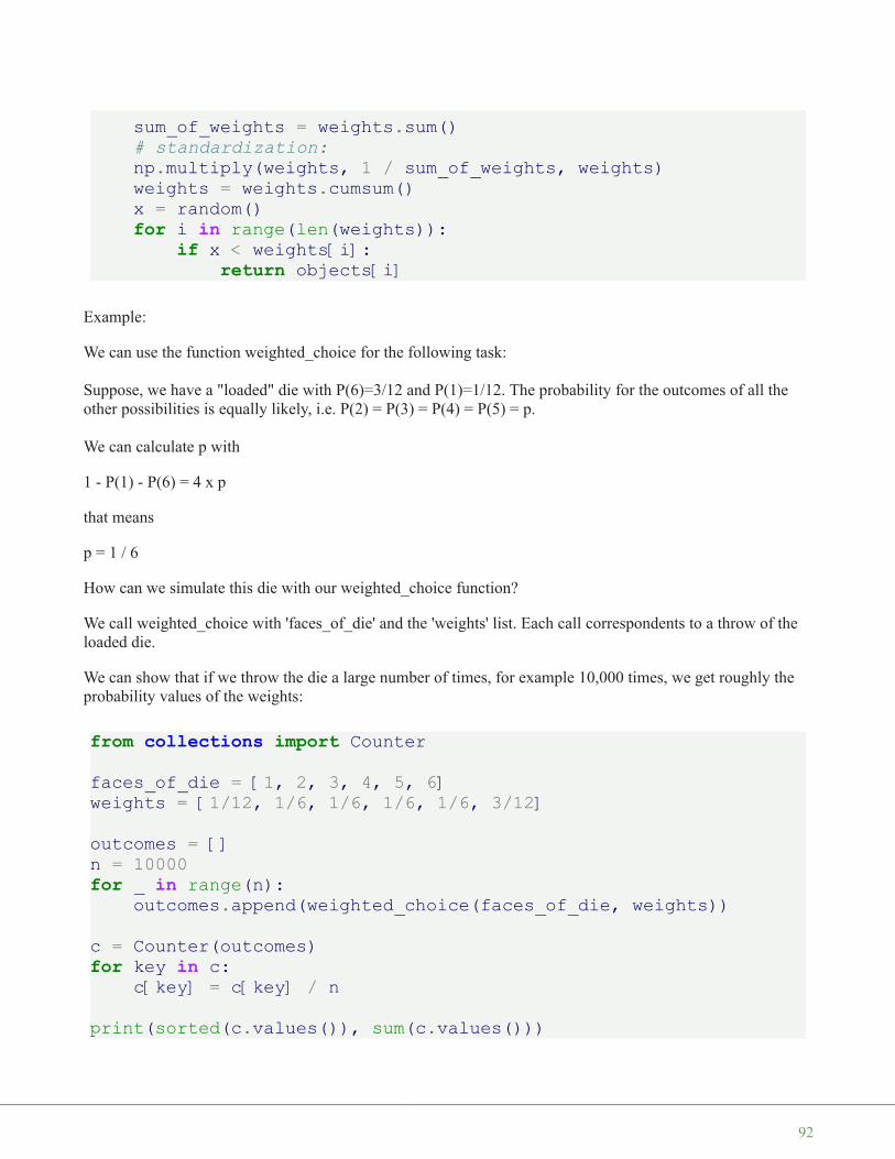
sum_of_weights = weights.sum()# standardization:np.multiply(weights, 1 / sum_of_weights, weights)weights = weights.cumsum()x = random()for i in range(len(weights)):

if x < weights[i]:return objects[i]

Example:

We can use the function weighted_choice for the following task:

Suppose, we have a "loaded" die with P(6)=3/12 and P(1)=1/12. The probability for the outcomes of all theother possibilities is equally likely, i.e. P(2) = P(3) = P(4) = P(5) = p.

We can calculate p with

1 - P(1) - P(6) = 4 x p

that means

p = 1 / 6

How can we simulate this die with our weighted_choice function?

We call weighted_choice with 'faces_of_die' and the 'weights' list. Each call correspondents to a throw of theloaded die.

We can show that if we throw the die a large number of times, for example 10,000 times, we get roughly theprobability values of the weights:

from collections import Counter

faces_of_die = [1, 2, 3, 4, 5, 6]weights = [1/12, 1/6, 1/6, 1/6, 1/6, 3/12]

outcomes = []n = 10000for _ in range(n):

outcomes.append(weighted_choice(faces_of_die, weights))

c = Counter(outcomes)for key in c:

c[key] = c[key] / n

print(sorted(c.values()), sum(c.values()))

92

We can also use list of strings with our 'weighted_choice' function.

We define a list of cities and a list with their corresponding populations. The probability of a city to be chosenshould be according to their size:

cities = ["Frankfurt","Stuttgart","Freiburg","München","Zürich","Hamburg"]

populations = [736000, 628000, 228000, 1450000, 409241, 1841179]total = sum(populations)weights = [ round(pop / total, 2) for pop in populations]print(weights)for i in range(10):

print(weighted_choice(cities, populations))

WEIGHTED RANDOM CHOICE WITH NUMPY

To produce a weighted choice of an array like object, we can also use the choice function of thenumpy.random package. Actually, you should use functions from well-established module like 'NumPy'instead of reinventing the wheel by writing your own code. In addition the 'choice' function from NumPy cando even more. It generates a random sample from a given 1-D array or array like object like a list, tuple and soon. The function can be called with four parameters:

choice(a, size=None, replace=True, p=None)

[0.0832, 0.1601, 0.1614, 0.1665, 0.1694, 0.2594] 1.0

[0.14, 0.12, 0.04, 0.27, 0.08, 0.35]FrankfurtHamburgStuttgartHamburgHamburgZürichMünchenStuttgartMünchenFrankfurt

93

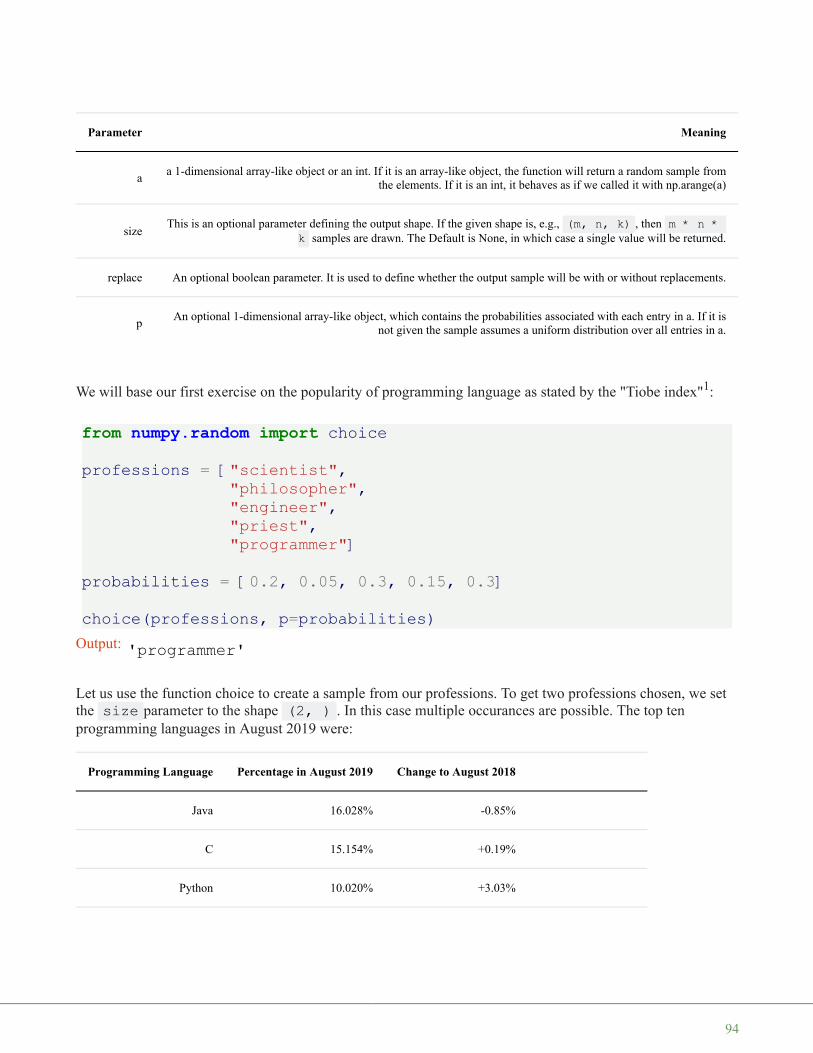
Parameter Meaning

aa 1-dimensional array-like object or an int. If it is an array-like object, the function will return a random sample from

the elements. If it is an int, it behaves as if we called it with np.arange(a)

sizeThis is an optional parameter defining the output shape. If the given shape is, e.g., (m, n, k) , then m * n *

k samples are drawn. The Default is None, in which case a single value will be returned.

replace An optional boolean parameter. It is used to define whether the output sample will be with or without replacements.

pAn optional 1-dimensional array-like object, which contains the probabilities associated with each entry in a. If it is

not given the sample assumes a uniform distribution over all entries in a.

We will base our first exercise on the popularity of programming language as stated by the "Tiobe index"1:

from numpy.random import choice

professions = ["scientist","philosopher","engineer","priest","programmer"]

probabilities = [0.2, 0.05, 0.3, 0.15, 0.3]

choice(professions, p=probabilities)

Let us use the function choice to create a sample from our professions. To get two professions chosen, we setthe size parameter to the shape (2, ) . In this case multiple occurances are possible. The top tenprogramming languages in August 2019 were:

Programming Language Percentage in August 2019 Change to August 2018

Java 16.028% -0.85%

C 15.154% +0.19%

Python 10.020% +3.03%

Output: 'programmer'

94

Programming Language Percentage in August 2019 Change to August 2018

C++ 6.057% -1.41%

C# 3.842% +0.30%

Visual Basic .NET 3.695% -1.07%

JavaScript 2.258% -0.15%

PHP 2.075% -0.85%

Objective-C 1.690% +0.33%

SQL 1.625% -0.69%

Ruby 1.316% +0.13%

programming_languages = ["Java", "C", "Python", "C++"]weights = np.array([16, 15.2, 10, 6.1])

# normalizationweights /= sum(weights)print(weights)

for i in range(10):print(choice(programming_languages, p=weights))

[0.33826638 0.32135307 0.21141649 0.12896406]JavaC++PythonPythonCC++CCPythonC

95

WEIGHTED SAMPLE

In the previous chapter on random numbers and probability, we introduced the function 'sample' of the module'random' to randomly extract a population or sample from a group of objects liks lists or tuples. Every objecthad the same likelikhood to be drawn, i.e. to be part of the sample.

In real life situation there will be of course situation in which every or some objects will have differentprobabilities. We will start again by defining a function on our own. This function will use the previouslydefined 'weighted_choice' function.

def weighted_sample(population, weights, k):"""This function draws a random sample (without repeats)of length k from the sequence 'population' accordingto the list of weights"""sample = set()population = list(population)weights = list(weights)while len(sample) < k:

choice = weighted_choice(population, weights)sample.add(choice)index = population.index(choice)weights.pop(index)population.remove(choice)weights = [ x / sum(weights) for x in weights]

return list(sample)

Example using the sample function:

Let's assume we have eight candies, coloured "red", "green", "blue", "yellow", "black", "white", "pink", and"orange". Our friend Peter will have the "weighted" preference 1/24, 1/6, 1/6, 1/12, 1/12, 1/24, 1/8, 7/24 forthes colours. He is allowed to take 3 candies:

candies = ["red", "green", "blue", "yellow", "black", "white", "pink", "orange"]weights = [ 1/24, 1/6, 1/6, 1/12, 1/12, 1/24, 1/8, 7/24]for i in range(10):

print(weighted_sample(candies, weights, 3))

96

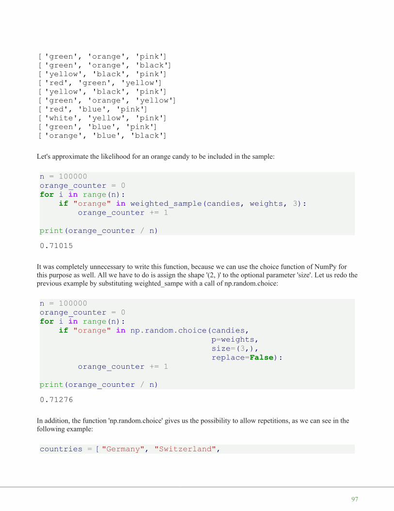
Let's approximate the likelihood for an orange candy to be included in the sample:

n = 100000orange_counter = 0for i in range(n):

if "orange" in weighted_sample(candies, weights, 3):orange_counter += 1

print(orange_counter / n)

It was completely unnecessary to write this function, because we can use the choice function of NumPy forthis purpose as well. All we have to do is assign the shape '(2, )' to the optional parameter 'size'. Let us redo theprevious example by substituting weighted_sampe with a call of np.random.choice:

n = 100000orange_counter = 0for i in range(n):

if "orange" in np.random.choice(candies,p=weights,size=(3,),replace=False):

orange_counter += 1

print(orange_counter / n)

In addition, the function 'np.random.choice' gives us the possibility to allow repetitions, as we can see in thefollowing example:

countries = ["Germany", "Switzerland",

['green', 'orange', 'pink']['green', 'orange', 'black']['yellow', 'black', 'pink']['red', 'green', 'yellow']['yellow', 'black', 'pink']['green', 'orange', 'yellow']['red', 'blue', 'pink']['white', 'yellow', 'pink']['green', 'blue', 'pink']['orange', 'blue', 'black']

0.71015

0.71276

97

"Austria", "Netherlands","Belgium", "Poland","France", "Ireland"]

weights = np.array([83019200, 8555541, 8869537,17338900, 11480534, 38413000,67022000, 4857000])

weights = weights / sum(weights)

for i in range(4):print(np.random.choice(countries,

p=weights,size=(3,),replace=True))

CARTESIAN CHOICE

The function cartesian_choice is named after the Cartesian product from set theory

CARTESIAN PRODUCT

The Cartesian product is an operation which returns a set from multiple sets. The result set from the Cartesianproduct is called a "product set" or simply the "product".

For two sets A and B, the Cartesian product A × B is the set of all ordered pairs (a, b) where a ∈ A and b ∈ B:

A x B = { (a, b) | a ∈ A and b ∈ B }

If we have n sets A1, A2, ... An, we can build the Cartesian product correspondingly:

A1 x A2 x ... x An = { (a1, a2, ... an) | a1 ∈ A1, a2 ∈ A2, ... an ∈ An]

The Cartesian product of n sets is sometimes called an n-fold Cartesian product.

CARTESIAN CHOICE: CARTESIAN_CHOICE

We will write now a function cartesian_choice, which takes an arbitrary number of iterables as arguments and

['Germany' 'Belgium' 'France']['Poland' 'Poland' 'Poland']['Germany' 'Austria' 'Poland']['France' 'France' 'France']

98

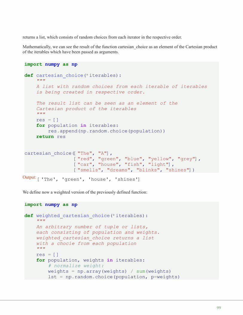
returns a list, which consists of random choices from each iterator in the respective order.

Mathematically, we can see the result of the function cartesian_choice as an element of the Cartesian productof the iterables which have been passed as arguments.

import numpy as npdef cartesian_choice(*iterables):

"""A list with random choices from each iterable of iterablesis being created in respective order.

The result list can be seen as an element of theCartesian product of the iterables"""res = []for population in iterables:

res.append(np.random.choice(population))return res

cartesian_choice(["The", "A"],["red", "green", "blue", "yellow", "grey"],["car", "house", "fish", "light"],["smells", "dreams", "blinks", "shines"])

We define now a weighted version of the previously defined function:

import numpy as npdef weighted_cartesian_choice(*iterables):

"""An arbitrary number of tuple or lists,each consisting of population and weights.weighted_cartesian_choice returns a listwith a chocie from each population"""res = []for population, weights in iterables:

# normalize weight:weights = np.array(weights) / sum(weights)lst = np.random.choice(population, p=weights)

Output: ['The', 'green', 'house', 'shines']

99

res.append(lst)return res

determiners = (["The", "A", "Each", "Every", "No"],[0.3, 0.3, 0.1, 0.1, 0.2])

colours = (["red", "green", "blue", "yellow", "grey"],[0.1, 0.3, 0.3, 0.2, 0.2])

nouns = (["water", "elephant", "fish", "light", "programming language"],

[0.3, 0.2, 0.1, 0.1, 0.3])nouns2 = (["of happiness", "of chocolate", "of wisdom", "of challenges", "of air"],

[0.5, 0.2, 0.1, 0.1, 0.1])verb_phrases = (["smells", "dreams", "thinks", "is made of"],

[0.4, 0.3, 0.2, 0.1])

print("It may or may not be true:")for i in range(10):

res = weighted_cartesian_choice(determiners,colours,nouns,verb_phrases,nouns2)

print(" ".join(res) + ".")

We check in the following version, if the "probabilities" are all right:

import randomdef weighted_cartesian_choice(*iterables):

"""A list with weighted random choices from each iterable of iter

ables

It may or may not be true:A grey light smells of happiness.The green water smells of happiness.A blue water smells of air.The green elephant dreams of happiness.A yellow fish smells of happiness.The grey elephant dreams of air.No grey programming language dreams of air.Every blue elephant smells of happiness.A blue light smells of air.The grey programming language dreams of happiness.

100

is being created in respective order"""res = []for population, weight in iterables:

lst = weighted_choice(population, weight)res.append(lst)

return res

determiners = (["The", "A", "Each", "Every", "No"],[0.3, 0.3, 0.1, 0.1, 0.2])

colours = (["red", "green", "blue", "yellow", "grey"],[0.1, 0.3, 0.3, 0.2, 0.2])

nouns = (["water", "elephant", "fish", "light", "programming language"],

[0.3, 0.2, 0.1, 0.1, 0.3])nouns2 = (["of happiness", "of chocolate", "of wisdom", "of challenges", "of air"],

[0.5, 0.2, 0.1, 0.1, 0.1])verb_phrases = (["smells", "dreams", "thinks", "is made of"],

[0.4, 0.3, 0.2, 0.1])

print("It may or may not be true:")sentences = []for i in range(10000):

res = weighted_cartesian_choice(determiners,colours,nouns,verb_phrases,nouns2)

sentences.append(" ".join(res) + ".")

words = ["smells", "dreams", "thinks", "is made of"]from collections import Counterc = Counter()for sentence in sentences:

for word in words:if word in sentence:

c[word] += 1

wsum = sum(c.values())for key in c:

print(key, c[key] / wsum)

101

RANDOM SEED

A random seed, - also called "seed state", or just "seed" - is a numberused to initialize a pseudorandom number generator. When we calledrandom.random() we expected and got a random number between 0and 1. random.random() calculates a new random number by using thepreviously produced random number. What about the first time we userandom in our program? Yes, there is no previously created randomnumber. If a random number generator is called for the first time, it willhave to create a first "random" number.

If we seed a pseudo-random number generator, we provide a first"previous" value. A seed value corresponds to a sequence of generatedvalues for a given random number generator. If you use the same seedvalue again, you get and you can rely on getting the same sequence ofnumbers again.

The seed number itself doesn't need to be randomly chosen so that thealgorithm creates values which follow a probability distribution in apseudorandom manner. Yet, the seed matters in terms of security. If youknow the seed, you could for example generate the secret encryption key which is based on this seed.

Random seeds are in many programming languages generated from the state of the computer system, which isin lots of cases the system time.

This is true for Python as well. Help on random.seed says that if you call the function with None or noargument it will seed "from current time or from an operating system specific randomness source if available."

import randomhelp(random.seed)

It may or may not be true:thinks 0.2015is made of 0.1039smells 0.4016dreams 0.293

102

The seed functions allows you to get a determined sequence of random numbers. You can repeat thissequence, whenever you need it again, e.g. for debugging purposes.

import randomrandom.seed(42)

for _ in range(10):print(random.randint(1, 10), end=", ")

print("\nLet's create the same random numbers again:")random.seed(42)for _ in range(10):

print(random.randint(1, 10), end=", ")

RANDOM NUMBERS IN PYTHON WITH GAUSSIAN AND NORMALVARIATEDISTRIBUTION

We want to create now 1000 random numbers between 130 and 230 that have a gaussian distribution with themean value mu set to 550 and the standard deviation sigma is set to 30.

Help on method seed in module random:

seed(a=None, version=2) method of random.Random instanceInitialize internal state from hashable object.

None or no argument seeds from current time or from an operating

system specific randomness source if available.

For version 2 (the default), all of the bits are used if *a* is a str,

bytes, or bytearray. For version 1, the hash() of *a* is used instead.

If *a* is an int, all bits are used.

2, 1, 5, 4, 4, 3, 2, 9, 2, 10,Let's create the same random numbers again:2, 1, 5, 4, 4, 3, 2, 9, 2, 10,

103

from random import gauss

n = 1000

values = []frequencies = {}

while len(values) < n:value = gauss(180, 30)if 130 < value < 230:

frequencies[int(value)] = frequencies.get(int(value), 0)+ 1

values.append(value)

print(values[:10])

The following program plots the random values, which we have created before. We haven't covered matplotlibso far, so it's not necessary to understand the code:

%matplotlib inline

import matplotlib.pyplot as pltfreq = list(frequencies.items())freq.sort()

plt.plot(*list(zip(*freq)))

[173.49123947564414, 183.47654360102564, 186.96893210720162, 214.90676059797428, 199.69909520396007, 183.31521532331496, 157.85035192965537, 149.56012897536849, 187.39026585633607, 219.33242481612143]

104

We do the same now with normvariate instead of gauss:

from random import normalvariate

n = 1000

values = []frequencies = {}

while len(values) < n:value = normalvariate(180, 30)if 130 < value < 230:

frequencies[int(value)] = frequencies.get(int(value), 0)+ 1

values.append(value)

freq = list(frequencies.items())freq.sort()

plt.plot(*list(zip(*freq)))

Output: [<matplotlib.lines.Line2D at 0x7f282554a828>]

105

EXERCISE WITH ZEROS AND ONES

It might be a good idea to write the following function as an exercise yourself. The function should be calledwith a parameter p, which is a probabilty value between 0 and 1. The function returns a 1 with a probability ofp, i.e. ones in p percent and zeros in (1 - p) percent of the calls:

import randomdef random_ones_and_zeros(p):

""" p: probability 0 <= p <= 1returns a 1 with the probability p

"""x = random.random()if x < p:

return 1else:

return 0

Let's test our little function:

n = 1000000sum(random_ones_and_zeros(0.8) for i in range(n)) / n

Output: [<matplotlib.lines.Line2D at 0x7f2824fef1d0>]

106

It might be a great idea to implement a task like this with a generator. If you are not familar with the way ofworking of a Python generator, we recommend to consult our chapter on generators and iterators of ourPython tutorial.

import randomdef random_ones_and_zeros(p):

while True:x = random.random()yield 1 if x < p else 0

def firstn(generator, n):for i in range(n):

yield next(generator)n = 1000000sum(x for x in firstn(random_ones_and_zeros(0.8), n)) / n

Our generator random_ones_and_zeros can be seen as a sender, which emits ones and zeros with a probabilityof p and (1-p) respectively.

We will write now another generator, which is receiving this bitstream. The task of this new generator is toread the incoming bitstream and yield another bitstream with ones and zeros with a probability of 0.5 without

knowing or using the probability p. It should work for an arbitrary probability value p.2

def ebitter(bitstream):while True:

bit1 = next(bitstream)

bit2 = next(bitstream)

if bit1 + bit2 ==1:

bit3 = next(bitstream)if bit2 + bit3 == 1:

yield 1else:

yield 0

def ebitter2(bitstream):

Output: 0.800609

Output: 0.799762

107

bit1 = next(bitstream)bit2 = next(bitstream)bit3 = next(bitstream)while True:

if bit1 + bit2 == 1:if bit2 + bit3 == 1:

yield 1else:

yield 0bit1, bit2, bit3 = bit2, bit3, next(bitstream)

n = 1000000sum(x for x in firstn(ebitter(random_ones_and_zeros(0.8)), n)) / n

n = 1000000sum(x for x in firstn(ebitter2(random_ones_and_zeros(0.8)), n)) /n

Underlying theory:

Our first generator emits a bitstream B0, B1, B2,...

We check now an arbitrary pair of consecutive Bits Bi, Bi+1, ...

Such a pair can have the values 01, 10, 00 or 11. The probability P(01) = (p-1) x p and probability P(10) = p x(p-1), so that the combined probabilty that the two consecutive bits are either 01 or 10 (or the sum of the twobits is 1) is 2 x (p-1) x p

Now we look at another bit Bi+2. What is the probability that both

Bi + Bi+1 = 1

and

Bi+1 + Bi+2 = 1?

The possible outcomes satisfying these conditions and their corresponding probabilities can be found in thefollowing table:

Probability Bi Bi+1 Bi+2

Output: 0.49975

Output: 0.500011

108

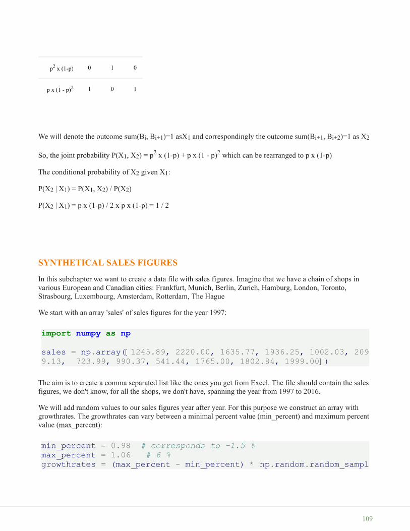
p2 x (1-p) 0 1 0

p x (1 - p)2 1 0 1

We will denote the outcome sum(Bi, Bi+1)=1 asX1 and correspondingly the outcome sum(Bi+1, Bi+2)=1 as X2

So, the joint probability P(X1, X2) = p2 x (1-p) + p x (1 - p)2 which can be rearranged to p x (1-p)

The conditional probability of X2 given X1:

P(X2 | X1) = P(X1, X2) / P(X2)

P(X2 | X1) = p x (1-p) / 2 x p x (1-p) = 1 / 2

SYNTHETICAL SALES FIGURES

In this subchapter we want to create a data file with sales figures. Imagine that we have a chain of shops invarious European and Canadian cities: Frankfurt, Munich, Berlin, Zurich, Hamburg, London, Toronto,Strasbourg, Luxembourg, Amsterdam, Rotterdam, The Hague

We start with an array 'sales' of sales figures for the year 1997:

import numpy as npsales = np.array([1245.89, 2220.00, 1635.77, 1936.25, 1002.03, 2099.13, 723.99, 990.37, 541.44, 1765.00, 1802.84, 1999.00])

The aim is to create a comma separated list like the ones you get from Excel. The file should contain the salesfigures, we don't know, for all the shops, we don't have, spanning the year from 1997 to 2016.

We will add random values to our sales figures year after year. For this purpose we construct an array withgrowthrates. The growthrates can vary between a minimal percent value (min_percent) and maximum percentvalue (max_percent):

min_percent = 0.98 # corresponds to -1.5 %max_percent = 1.06 # 6 %growthrates = (max_percent - min_percent) * np.random.random_sampl

109

e(12) + min_percentprint(growthrates)

To get the new sales figures after a year, we multiply the sales array "sales" with the array "growthrates":

sales * growthrates

To get a more sustainable sales development, we change the growthrates only every four years.

This is our complete program, which saves the data in a file called sales_figures.csv:

import numpy as npfh = open("sales_figures.csv", "w")

fh.write("Year, Frankfurt, Munich, Berlin, Zurich, Hamburg, London, Toronto, Strasbourg, Luxembourg, Amsterdam, Rotterdam, The Hague\n")sales = np.array([1245.89, 2220.00, 1635.77, 1936.25, 1002.03, 2099.13, 723.99, 990.37, 541.44, 1765.00, 1802.84, 1999.00])

for year in range(1997, 2016):line = str(year) + ", " + ", ".join(map(str, sales))fh.write(line + "\n")if year % 4 == 0:

min_percent = 0.98 # corresponds to -1.5 %max_percent = 1.06 # 6 %growthrates = (max_percent - min_percent) * np.random.ran

dom_sample(12) + min_percent#growthrates = 1 + (np.random.rand(12) * max_percent - ne

gative_max) / 100sales = np.around(sales * growthrates, 2)

fh.close()

[ 1.03476561 1.00885095 1.00614899 1.05164581 1.0307091 0.98822763

0.99366872 1.05810125 1.04798573 1.02784796 1.05035899 1.02262023]

Output: array([ 1289.20412146, 2239.649113 , 1645.82833205, 2036.24919608,

1032.80143634, 2074.41825668, 719.40621318, 1047.91173209,

567.42139317, 1814.15165757, 1893.62920988, 2044.21783979])

110

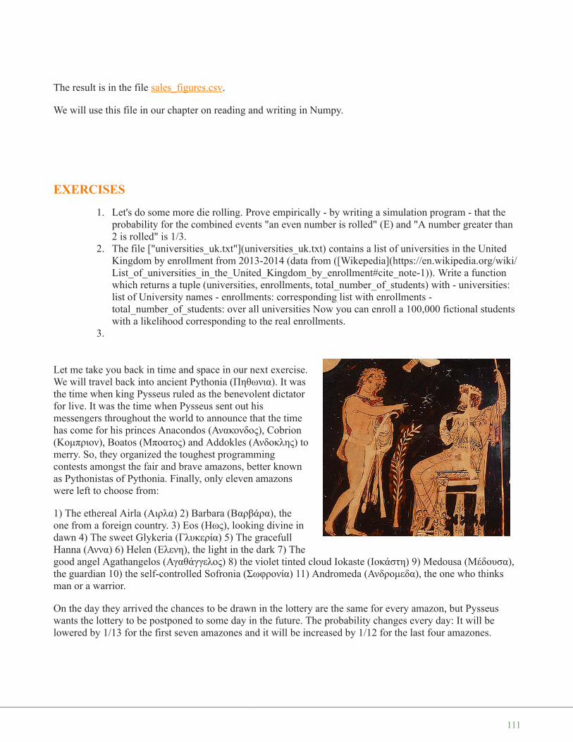
The result is in the file sales_figures.csv.

We will use this file in our chapter on reading and writing in Numpy.

EXERCISES

1. Let's do some more die rolling. Prove empirically - by writing a simulation program - that theprobability for the combined events "an even number is rolled" (E) and "A number greater than2 is rolled" is 1/3.

2. The file ["universities_uk.txt"](universities_uk.txt) contains a list of universities in the UnitedKingdom by enrollment from 2013-2014 (data from ([Wikepedia](https://en.wikipedia.org/wiki/List_of_universities_in_the_United_Kingdom_by_enrollment#cite_note-1)). Write a functionwhich returns a tuple (universities, enrollments, total_number_of_students) with - universities:list of University names - enrollments: corresponding list with enrollments -total_number_of_students: over all universities Now you can enroll a 100,000 fictional studentswith a likelihood corresponding to the real enrollments.

3.

Let me take you back in time and space in our next exercise.We will travel back into ancient Pythonia (Πηθωνια). It wasthe time when king Pysseus ruled as the benevolent dictatorfor live. It was the time when Pysseus sent out hismessengers throughout the world to announce that the timehas come for his princes Anacondos (Ανακονδος), Cobrion(Κομπριον), Boatos (Μποατος) and Addokles (Ανδοκλης) tomerry. So, they organized the toughest programmingcontests amongst the fair and brave amazons, better knownas Pythonistas of Pythonia. Finally, only eleven amazonswere left to choose from:

1) The ethereal Airla (Αιρλα) 2) Barbara (Βαρβάρα), theone from a foreign country. 3) Eos (Ηως), looking divine indawn 4) The sweet Glykeria (Γλυκερία) 5) The gracefullHanna (Αννα) 6) Helen (Ελενη), the light in the dark 7) Thegood angel Agathangelos (Αγαθάγγελος) 8) the violet tinted cloud Iokaste (Ιοκάστη) 9) Medousa (Μέδουσα),the guardian 10) the self-controlled Sofronia (Σωφρονία) 11) Andromeda (Ανδρομεδα), the one who thinksman or a warrior.

On the day they arrived the chances to be drawn in the lottery are the same for every amazon, but Pysseuswants the lottery to be postponed to some day in the future. The probability changes every day: It will belowered by 1/13 for the first seven amazones and it will be increased by 1/12 for the last four amazones.

111

How long will the king have to wait until he can be more than 90 percent sure that his princes Anacondos,Cobrion, Boatos and Addokles will be married to Iokaste, Medousa, Sofronia and Andromeda?

</li>

</ol>

SOLUTIONS TO OUR EXERCISES1.

from random import randint

outcomes = [ randint(1, 6) for _ in range(10000)]

even_pips = [ x for x in outcomes if x % 2 == 0]greater_two = [ x for x in outcomes if x > 2]

combined = [ x for x in outcomes if x % 2 == 0 and x > 2]

print(len(even_pips) / len(outcomes))print(len(greater_two) / len(outcomes))print(len(combined) / len(outcomes))

• At first we will write the function "process_datafile" to process our data file:

def process_datafile(filename):""" process_datafile -> (universities,

enrollments,total_number_of_students)

universities: list of University namesenrollments: corresponding list with enrollmentstotal_number_of_students: over all universities

"""

universities = []enrollments = []with open(filename) as fh:

0.50610.67190.3402

112

total_number_of_students = 0fh.readline() # get rid of descriptive first linefor line in fh:

line = line.strip()*praefix, undergraduates, postgraduates, total = lin

e.rsplit()university = praefix[1:]total = int(total.replace(",", ""))enrollments.append(total)universities.append(" ".join(university))total_number_of_students += total

return (universities, enrollments, total_number_of_students)

Let's start our function and check the results:

universities, enrollments, total_students = process_datafile("universities_uk.txt")

for i in range(14):print(universities[i], end=": ")print(enrollments[i])

print("Total number of students onrolled in the UK: ", total_students)

We want to enroll now a virtual student randomly to one of the universities. To get a weighted list suitable forour weighted_choice function, we have to normalize the values in the list enrollments:

normalized_enrollments = [ students / total_students for students

Open University in England: 123490University of Manchester: 37925University of Nottingham: 33270Sheffield Hallam University: 33100University of Birmingham: 32335Manchester Metropolitan University: 32160University of Leeds: 30975Cardiff University: 30180University of South Wales: 29195University College London: 28430King's College London: 27645University of Edinburgh: 27625Northumbria University: 27565University of Glasgow: 27390Total number of students onrolled in the UK: 2299380

113

in enrollments]

# enrolling a virtual student:print(weighted_choice(universities, normalized_enrollments))

We have been asked by the exercise to "enroll" 100,000 fictional students. This can be easily accomplishedwith a loop:

from collections import Counter

outcomes = []n = 100000for i in range(n):

outcomes.append(weighted_choice(universities, normalized_enrollments))

c = Counter(outcomes)

print(c.most_common(20))

</li>•

The bunch of amazons is implemented as a list, while we choose a set for Pysseusses favorites. The weights atthe beginning are 1/11 for all, i.e. 1/len(amazons).

Every loop cycle corresponds to a new day. Every time we start a new loop cycle, we will draw "n" samples ofPythonistas to calculate the ratio of the number of times the sample is equal to the king's favorites divided bythe number of times the sample doesn't match the king's idea of daughter-in-laws. This corresponds to the

University of Dundee

[('Open University in England', 5529), ('University of Manchester', 1574), ('University of Nottingham', 1427), ('University of Birmingham', 1424), ('Sheffield Hallam University', 1410), ('Manchester Metropolitan University', 1408), ('Cardiff University', 1334),('University of Leeds', 1312), ('University of South Wales', 1264), ('University of Plymouth', 1218), ('University College London', 1209), ('Coventry University', 1209), ('University of the West of England', 1197), ('University of Edinburgh', 1196), ("King'sCollege London", 1183), ('University of Glasgow', 1181), ('University of Central Lancashire', 1176), ('Nottingham Trent University', 1174), ('University of Sheffield', 1160), ('Northumbria University', 1154)]

114

probability "prob". We stop the first time, the probability is equal or larger than 0.9.

We can use both the function "weighted_same" and "weighted_sample_alternative" to do the drawing.

import timeamazons = ["Airla", "Barbara", "Eos",

"Glykeria", "Hanna", "Helen","Agathangelos", "Iokaste","Medousa", "Sofronia","Andromeda"]

weights = [ 1/len(amazons) for _ in range(len(amazons)) ]

Pytheusses_favorites = {"Iokaste", "Medousa","Sofronia", "Andromeda"}

n = 1000counter = 0

prob = 1 / 330days = 0factor1 = 1 / 13factor2 = 1 / 12

start = time.clock()while prob < 0.9:

for i in range(n):the_chosen_ones = weighted_sample_alternative(amazons, wei

ghts, 4)if set(the_chosen_ones) == Pytheusses_favorites:

counter += 1prob = counter / ncounter = 0weights[:7] = [ p - p*factor1 for p in weights[:7] ]weights[7:] = [ p + p*factor2 for p in weights[7:] ]weights = [ x / sum(weights) for x in weights]days += 1

print(time.clock() - start)

print("Number of days, he has to wait: ", days)2.870792999999999Number of days, he has to wait: 33

115

Teh value for the number of days differs, if n is not large enough.

The following is a solutions without round-off errors. We will use Fraction from the module fractions.

import timefrom fractions import Fraction

amazons = ["Airla", "Barbara", "Eos","Glykeria", "Hanna", "Helen","Agathangelos", "Iokaste","Medousa", "Sofronia","Andromeda"]

weights = [ Fraction(1, 11) for _ in range(len(amazons)) ]

Pytheusses_favorites = {"Iokaste", "Medousa","Sofronia", "Andromeda"}

n = 1000counter = 0

prob = Fraction(1, 330)days = 0factor1 = Fraction(1, 13)factor2 = Fraction(1, 12)

start = time.clock()while prob < 0.9:

#print(prob)for i in range(n):

the_chosen_ones = weighted_sample_alternative(amazons, weights, 4)

if set(the_chosen_ones) == Pytheusses_favorites:counter += 1

prob = Fraction(counter, n)counter = 0weights[:7] = [ p - p*factor1 for p in weights[:7] ]weights[7:] = [ p + p*factor2 for p in weights[7:] ]weights = [ x / sum(weights) for x in weights]days += 1

print(time.clock() - start)

print("Number of days, he has to wait: ", days)

116

We can see that the solution with fractions is beautiful but very slow. Whereas the greater precision doesn'tplay a role in our case.

So far, we haven't used the power of Numpy. We will do this in the next implementation of our problem:

import timeimport numpy as npamazons = ["Airla", "Barbara", "Eos",

"Glykeria", "Hanna", "Helen","Agathangelos", "Iokaste","Medousa", "Sofronia","Andromeda"]

weights = np.full(11, 1/len(amazons))

Pytheusses_favorites = {"Iokaste", "Medousa","Sofronia", "Andromeda"}

n = 1000counter = 0

prob = 1 / 330days = 0factor1 = 1 / 13factor2 = 1 / 12

start = time.clock()while prob < 0.9:

for i in range(n):the_chosen_ones = weighted_sample_alternative(amazons, wei

ghts, 4)if set(the_chosen_ones) == Pytheusses_favorites:

counter += 1prob = counter / ncounter = 0weights[:7] = weights[:7] - weights[:7] * factor1weights[7:] = weights[7:] + weights[7:] * factor2weights = weights / np.sum(weights)

35.920345Number of days, he has to wait: 33

117

#print(weights)days += 1

print(time.clock() - start)

print("Number of days, he has to wait: ", days)

FOOTNOTES:

1 The TIOBE index or The TIOBE Programming Community index is - according to the website "an indicatorof the popularity of programming languages. The index is updated once a month. The ratings are based on thenumber of skilled engineers world-wide, courses and third party vendors. Popular search engines such asGoogle, Bing, Yahoo!, Wikipedia, Amazon, YouTube and Baidu are used to calculate the ratings. It isimportant to note that the TIOBE index is not about the best programming language or the language in whichmost lines of code have been written."

2 I am thankful to Dr. Hanno Baehr who introduced me to the problem of "Random extraction" whenparticipating in a Python training course in Nuremberg in January 2014. Hanno outlined some bits of thetheoretical framework. During a night session in a pub called "Zeit & Raum" (english: "Time & Space") Iimplemented a corresponding Python program to back the theoretical solution empirically.

4.930090000000007Number of days, he has to wait: 33

118

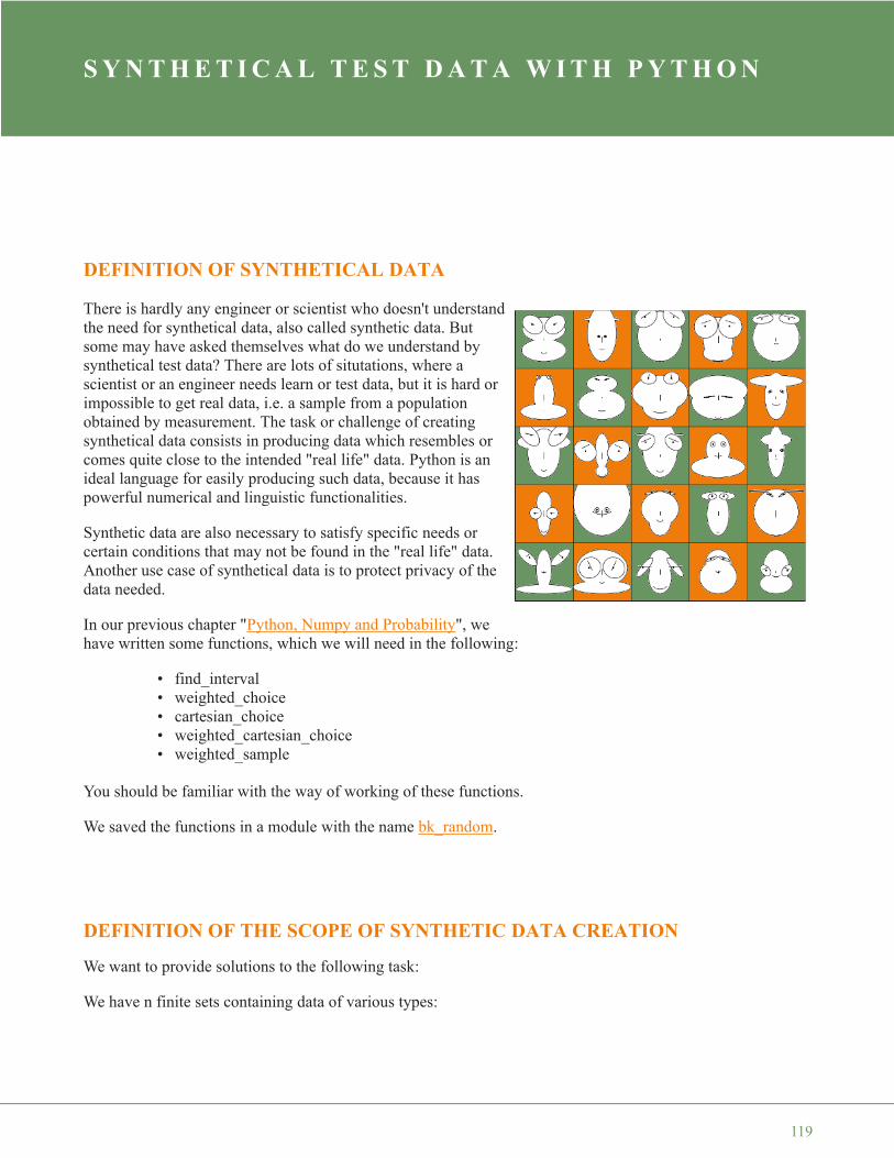
S Y N T H E T I C A L T E S T D A T A W I T H P Y T H O N

DEFINITION OF SYNTHETICAL DATA

There is hardly any engineer or scientist who doesn't understandthe need for synthetical data, also called synthetic data. Butsome may have asked themselves what do we understand bysynthetical test data? There are lots of situtations, where ascientist or an engineer needs learn or test data, but it is hard orimpossible to get real data, i.e. a sample from a populationobtained by measurement. The task or challenge of creatingsynthetical data consists in producing data which resembles orcomes quite close to the intended "real life" data. Python is anideal language for easily producing such data, because it haspowerful numerical and linguistic functionalities.

Synthetic data are also necessary to satisfy specific needs orcertain conditions that may not be found in the "real life" data.Another use case of synthetical data is to protect privacy of thedata needed.

In our previous chapter "Python, Numpy and Probability", wehave written some functions, which we will need in the following:

• find_interval• weighted_choice• cartesian_choice• weighted_cartesian_choice• weighted_sample

You should be familiar with the way of working of these functions.

We saved the functions in a module with the name bk_random.

DEFINITION OF THE SCOPE OF SYNTHETIC DATA CREATION

We want to provide solutions to the following task:

We have n finite sets containing data of various types:

119

D1, D2, ... Dn

The sets Di are the data sets from which we want to deduce our synthetical data.

In the actual implementation, the sets will be tuples or lists for practical reasons.

The process of creating synthetic data can be defined by two functions "synthesizer" and "synthesize".Usually, the word synthesizer is used for a computerized electronic device which produces sound. Oursynthesizer produces strings or alternatively tuples with data, as we will see later.

The function synthesizer creates the function synthesize:

synthesize = synthesizer( (D1, D2, ... Dn) )

The function synthesize, - which may also be a generator like in our implementation, - takes no arguments andthe result of a function call sythesize() will be

• a list or a tuple t = (d1, d2, ... dn) where di is drawn at random from Di• or a string which contains the elements str(d1), str(d2), ... str(dn) where di is also drawn at

random from Di

Let us start with a simple example. We have a list of firstnames and a list of surnames. We want to hireemployees for an institute or company. Of course, it will be a lot easier in our synthetical Python environmentto find and hire specialsts than in real life. The function "cartesian_choice" from the bk_random module andthe concatenation of the randomly drawn firstnames and surnames is all it takes.

import bk_randomfirstnames = ["John", "Eve", "Jane", "Paul",

"Frank", "Laura", "Robert","Kathrin", "Roger", "Simone","Bernard", "Sarah", "Yvonne"]

surnames = ["Singer", "Miles", "Moore","Looper", "Rampman", "Chopman","Smiley", "Bychan", "Smith","Baker", "Miller", "Cook"]

number_of_specialists = 15

employees = set()while len(employees) < number_of_specialists:

employee = bk_random.cartesian_choice(firstnames, surnames)employees.add(" ".join(employee))

print(employees)

120

This was easy enough, but we want to do it now in a more structured way, using the synthesizer approach wementioned before. The code for the case in which the parameter "weights" is not None is still missing in thefollowing implementation:

import bk_randomfirstnames = ["John", "Eve", "Jane", "Paul",

"Frank", "Laura", "Robert","Kathrin", "Roger", "Simone","Bernard", "Sarah", "Yvonne"]

surnames = ["Singer", "Miles", "Moore","Looper", "Rampman", "Chopman","Smiley", "Bychan", "Smith","Baker", "Miller", "Cook"]

def synthesizer( data, weights=None, format_func=None, repeats=True):

"""data is a tuple or list of lists or tuples containing thedataweights is a list or tuple of lists or tuples with thecorresponding weights of the data lists or tuplesformat_func is a reference to a function which defineshow a random result of the creator function will be formated.If None, "creator" will return the list "res".If repeats is set to True, the results of helper will not be u

nique"""

def synthesize():if not repeats:

memory = set()while True:

res = bk_random.cartesian_choice(*data)if not repeats:

sres = str(res)while sres in memory:

res = bk_random.cartesian_choice(*data)sres = str(res)

{'Laura Smith', 'Yvonne Miles', 'Sarah Cook', 'Jane Smith', 'PaulMoore', 'Jane Miles', 'Jane Looper', 'Frank Singer', 'Frank Miles', 'Jane Cook', 'Frank Chopman', 'Laura Cook', 'Yvonne Bychan','Eve Miles', 'Simone Cook'}

121

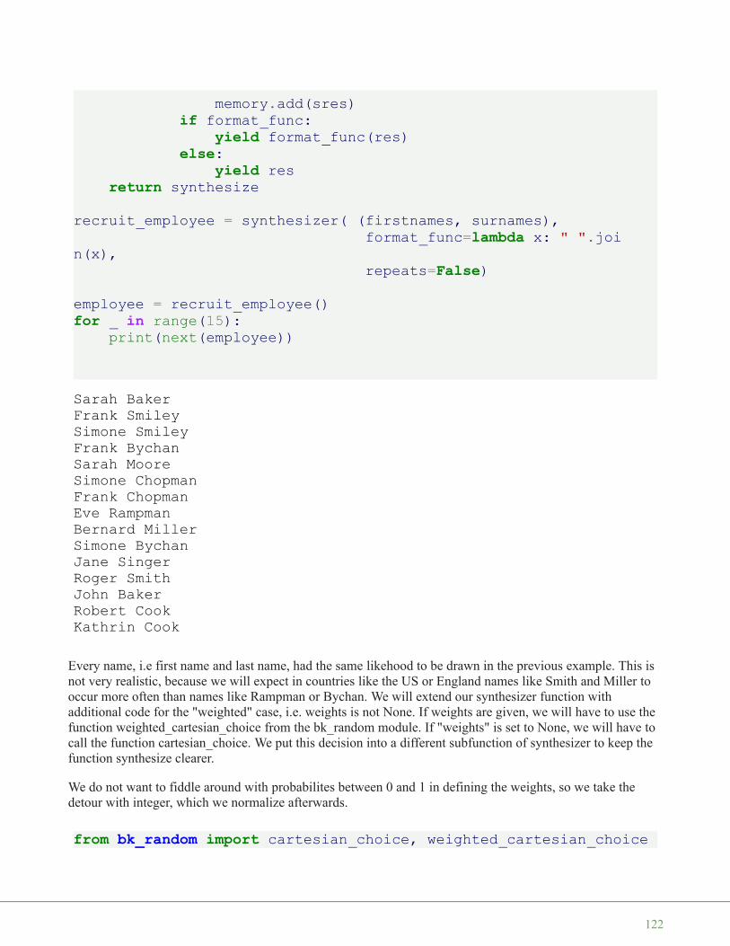
memory.add(sres)if format_func:

yield format_func(res)else:

yield resreturn synthesize

recruit_employee = synthesizer( (firstnames, surnames),format_func=lambda x: " ".joi

n(x),repeats=False)

employee = recruit_employee()for _ in range(15):

print(next(employee))

Every name, i.e first name and last name, had the same likehood to be drawn in the previous example. This isnot very realistic, because we will expect in countries like the US or England names like Smith and Miller tooccur more often than names like Rampman or Bychan. We will extend our synthesizer function withadditional code for the "weighted" case, i.e. weights is not None. If weights are given, we will have to use thefunction weighted_cartesian_choice from the bk_random module. If "weights" is set to None, we will have tocall the function cartesian_choice. We put this decision into a different subfunction of synthesizer to keep thefunction synthesize clearer.

We do not want to fiddle around with probabilites between 0 and 1 in defining the weights, so we take thedetour with integer, which we normalize afterwards.

from bk_random import cartesian_choice, weighted_cartesian_choice

Sarah BakerFrank SmileySimone SmileyFrank BychanSarah MooreSimone ChopmanFrank ChopmanEve RampmanBernard MillerSimone BychanJane SingerRoger SmithJohn BakerRobert CookKathrin Cook

122

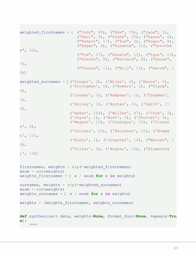
weighted_firstnames = [ ("John", 80), ("Eve", 70), ("Jane", 2),("Paul", 8), ("Frank", 20), ("Laura", 6),("Robert", 17), ("Zoe", 3), ("Roger", 8),("Edgar", 4), ("Susanne", 11), ("Dorothe

e", 22),("Tim", 17), ("Donald", 12), ("Igor", 15),("Simone", 9), ("Bernard", 8), ("Sarah",

7),("Yvonne", 11), ("Bill", 12), ("Bernd", 1

0)]

weighted_surnames = [('Singer', 2), ('Miles', 2), ('Moore', 5),('Strongman', 5), ('Romero', 3), ("Yiang",

4),('Looper', 1), ('Rampman', 1), ('Chopman',

1),('Smiley', 1), ('Bychan', 1), ('Smith', 15

0),('Baker', 144), ('Miller', 87), ('Cook', 5),('Joyce', 1), ('Bush', 5), ('Shorter', 6),('Wagner', 10), ('Sundigos', 10), ('Firenz

e', 8),('Puttner', 20), ('Faulkner', 10), ('Bowma

n', 11),('Klein', 1), ('Jungster', 14), ("Warner", 1

4),('Tiller', 9), ('Wogner', 10), ('Blumentha

l', 16)]

firstnames, weights = zip(*weighted_firstnames)wsum = sum(weights)weights_firstnames = [ x / wsum for x in weights]

surnames, weights = zip(*weighted_surnames)wsum = sum(weights)weights_surnames = [ x / wsum for x in weights]

weights = (weights_firstnames, weights_surnames)

def synthesizer( data, weights=None, format_func=None, repeats=True):

"""

123

"data" is a tuple or list of lists or tuples containing thedata.

"weights" is a list or tuple of lists or tuples with thecorresponding weights of the data lists or tuples.

"format_func" is a reference to a function which defineshow a random result of the creator function will be formated.If None,the generator "synthesize" will yield the list "res".

If "repeats" is set to True, the output values yielded by"synthesize" will not be unique."""

def choice(data, weights):if weights:

return weighted_cartesian_choice(*zip(data, weights))else:

return cartesian_choice(*data)

def synthesize():if not repeats:

memory = set()while True:

res = choice(data, weights)if not repeats:

sres = str(res)while sres in memory:

res = choice(data, weights)sres = str(res)

memory.add(sres)if format_func:

yield format_func(res)else:

yield resreturn synthesize

recruit_employee = synthesizer( (firstnames, surnames),weights = weights,format_func=lambda x: " ".join(x),repeats=False)

employee = recruit_employee()

124

for _ in range(12):print(next(employee))

WINE EXAMPLE

Let's imagine that you have to describe a dozen wines. Mostprobably a nice imagination for many, but I have to admit that itis not for me. The main reason is that I am not a wine drinker!

We can write a little Python program, which will use oursynthesize function to create automatically "sophisticatedcriticisms" like this one:

This wine is light-bodied with a conveniently juicy bouquetleading to a lingering flamboyant finish!

Try to find some adverbs, like "seamlessly", "assertively", andsome adjectives, like "fruity" and "refined", to describe thearoma.

If you have defined your lists, you can use the synthesizefunction.

Here is our solution, in case you don't want to do it on your own:

import bk_randombody = ['light-bodied', 'medium-bodied', 'full-bodied']

adverbs = ['appropriately', 'assertively', 'authoritatively','compellingly', 'completely', 'continually',

Frank BakerFrank SmithEve SmithDorothee BakerJohn SmithBill BushJohn SundigosLaura BlumenthalZoe SmithIgor BakerBill MillerEve Baker

125

'conveniently', 'credibly', 'distinctively','dramatically', 'dynamically', 'efficiently','energistically', 'enthusiastically', 'fungibly','globally', 'holisticly', 'interactively','intrinsically', 'monotonectally', 'objectively','phosfluorescently', 'proactively', 'professionally','progressively', 'quickly', 'rapidiously','seamlessly', 'synergistically', 'uniquely']

noun = ['aroma', 'bouquet', 'flavour']

aromas = ['angular', 'bright', 'lingering', 'butterscotch','buttery', 'chocolate', 'complex', 'earth', 'flabby','flamboyant', 'fleshy', 'flowers', 'food friendly','fruits', 'grass', 'herbs', 'jammy', 'juicy', 'mocha','oaked', 'refined', 'structured', 'tight', 'toast','toasty', 'tobacco', 'unctuous', 'unoaked', 'vanilla','velvetly']

example = """This wine is light-bodied with a completely butterybouquet leading to a lingering fruity finish!"""

def describe(data):body, adv, adj, noun, adj2 = dataformat_str = "This wine is %s with a %s %s %s\nleading to"format_str += " a lingering %s finish!"return format_str % (body, adv, adj, noun, adj2)

t = bk_random.cartesian_choice(body, adverbs, aromas, noun, aromas)

data = (body, adverbs, aromas, noun, aromas)synthesize = synthesizer( data, weights=None, format_func=describe, repeats=True)criticism = synthesize()

for i in range(1, 13):print("{0:d}. wine:".format(i))print(next(criticism))print()

126

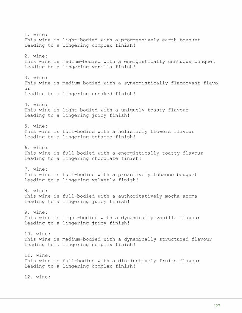
1. wine:This wine is light-bodied with a progressively earth bouquetleading to a lingering complex finish!

2. wine:This wine is medium-bodied with a energistically unctuous bouquetleading to a lingering vanilla finish!

3. wine:This wine is medium-bodied with a synergistically flamboyant flavourleading to a lingering unoaked finish!

4. wine:This wine is light-bodied with a uniquely toasty flavourleading to a lingering juicy finish!

5. wine:This wine is full-bodied with a holisticly flowers flavourleading to a lingering tobacco finish!

6. wine:This wine is full-bodied with a energistically toasty flavourleading to a lingering chocolate finish!

7. wine:This wine is full-bodied with a proactively tobacco bouquetleading to a lingering velvetly finish!

8. wine:This wine is full-bodied with a authoritatively mocha aromaleading to a lingering juicy finish!

9. wine:This wine is light-bodied with a dynamically vanilla flavourleading to a lingering juicy finish!

10. wine:This wine is medium-bodied with a dynamically structured flavourleading to a lingering complex finish!

11. wine:This wine is full-bodied with a distinctively fruits flavourleading to a lingering complex finish!

12. wine:

127

EXERCISE: INTERNATIONAL DISASTER OPERATION

It would be gorgeous, if the problem described in this exercise,would be purely synthetic, i.e. there would be no furthercatastophes in the world. Completely unrealistic, but a nicedaydream. So, the task of this exercise is to provide syntheticaltest data for an international disaster operation. The countriestaking part in this mission might be e.g. France, Switzerland,Germany, Canada, The Netherlands, The United States, Austria,Belgium and Luxembourg.

We want to create a file with random entries of aides. Each lineshould consist of:

UniqueIdentifier, FirstName, LastName, Country, Field

For example:

001, Jean-Paul, Rennier, France, Medical Aid002, Nathan, Bloomfield, Canada, Security Aid003, Michael, Mayer, Germany, Social Worker

For practical reasons, we will reduce the countries to France, Italy, Switzerland and Germany in the followingexample implementation:

from bk_random import cartesian_choice, weighted_cartesian_choice

countries = ["France", "Switzerland", "Germany"]

w_firstnames = { "France" : [ ("Marie", 10), ("Thomas", 10),("Camille", 10), ("Nicolas", 9),("Léa", 10), ("Julien", 9),("Manon", 9), ("Quentin", 9),("Chloé", 8), ("Maxime", 9),("Laura", 7), ("Alexandre", 6),("Clementine", 2), ("Grégory", 2),("Sandra", 1), ("Philippe", 1)],

"Switzerland": [ ("Sarah", 10), ("Hans", 10),("Laura", 9), ("Peter", 8),

This wine is medium-bodied with a conveniently tight aromaleading to a lingering chocolate finish!

128

("Mélissa", 9), ("Walter", 7),("Océane", 7), ("Daniel", 7),("Noémie", 6), ("Reto", 7),("Laura", 7), ("Bruno", 6),("Eva", 2), ("Urli", 4),("Sandra", 1), ("Marcel", 1)],

"Germany": [ ("Ursula", 10), ("Peter", 10),("Monika", 9), ("Michael", 8),("Brigitte", 9), ("Thomas", 7),("Stefanie", 7), ("Andreas", 7),("Maria", 6), ("Wolfgang", 7),("Gabriele", 7), ("Manfred", 6),("Nicole", 2), ("Matthias", 4),("Christine", 1), ("Dirk", 1)],

"Italy" : [ ("Francesco", 20), ("Alessandro", 19),("Mattia", 19), ("Lorenzo", 18),("Leonardo", 16), ("Andrea", 15),("Gabriele", 14), ("Matteo", 14),("Tommaso", 12), ("Riccardo", 11),("Sofia", 20), ("Aurora", 18),("Giulia", 16), ("Giorgia", 15),("Alice", 14), ("Martina", 1

3)]}

w_surnames = { "France" : [ ("Matin", 10), ("Bernard", 10),("Camille", 10), ("Nicolas", 9),("Dubois", 10), ("Petit", 9),

("Durand", 8), ("Leroy", 8),("Fournier", 7), ("Lambert", 6),("Mercier", 5), ("Rousseau", 4),("Mathieu", 2), ("Fontaine", 2),("Muller", 1), ("Robin", 1)],

"Switzerland": [ ("Müller", 10), ("Meier", 10),("Schmid", 9), ("Keller", 8),("Weber", 9), ("Huber", 7),("Schneider", 7), ("Meyer", 7),("Steiner", 6), ("Fischer", 7),("Gerber", 7), ("Brunner", 6),("Baumann", 2), ("Frei", 4),("Zimmermann", 1), ("Moser", 1)],

"Germany": [ ("Müller", 10), ("Schmidt", 10),("Schneider", 9), ("Fischer", 8),("Weber", 9), ("Meyer", 7),("Wagner", 7), ("Becker", 7),

129

("Schulz", 6), ("Hoffmann", 7),("Schäfer", 7), ("Koch", 6),("Bauer", 2), ("Richter", 4),("Klein", 2), ("Schröder", 1)],

"Italy" : [ ("Rossi", 20), ("Russo", 19),("Ferrari", 19), ("Esposito", 18),("Bianchi", 16), ("Romano", 15),("Colombo", 14), ("Ricci", 14),("Marino", 12), ("Grecco", 11),("Bruno", 10), ("Gallo", 12),("Conti", 16), ("De Luca", 15),("Costa", 14), ("Giordano", 13),("Mancini", 14), ("Rizzo", 13),("Lombardi", 11), ("Moretto", 9)]}

# separate names and weightssynthesize = {}identifier = 1for country in w_firstnames:

firstnames, weights = zip(*w_firstnames[country])wsum = sum(weights)weights_firstnames = [ x / wsum for x in weights]w_firstnames[country] = [firstnames, weights_firstnames]

surnames, weights = zip(*w_surnames[country])wsum = sum(weights)weights_surnames = [ x / wsum for x in weights]w_surnames[country] = [surnames, weights_firstnames]

synthesize[country] = synthesizer( (firstnames, surnames),(weights_firstnames,weights_surnames),

format_func=lambda x: " ".join(x),

repeats=False)nation_prob = [("Germany", 0.3),

("France", 0.4),("Switzerland", 0.2),("Italy", 0.1)]

profession_prob = [("Medical Aid", 0.3),("Social Worker", 0.6),("Security Aid", 0.1)]

helpers = []

130

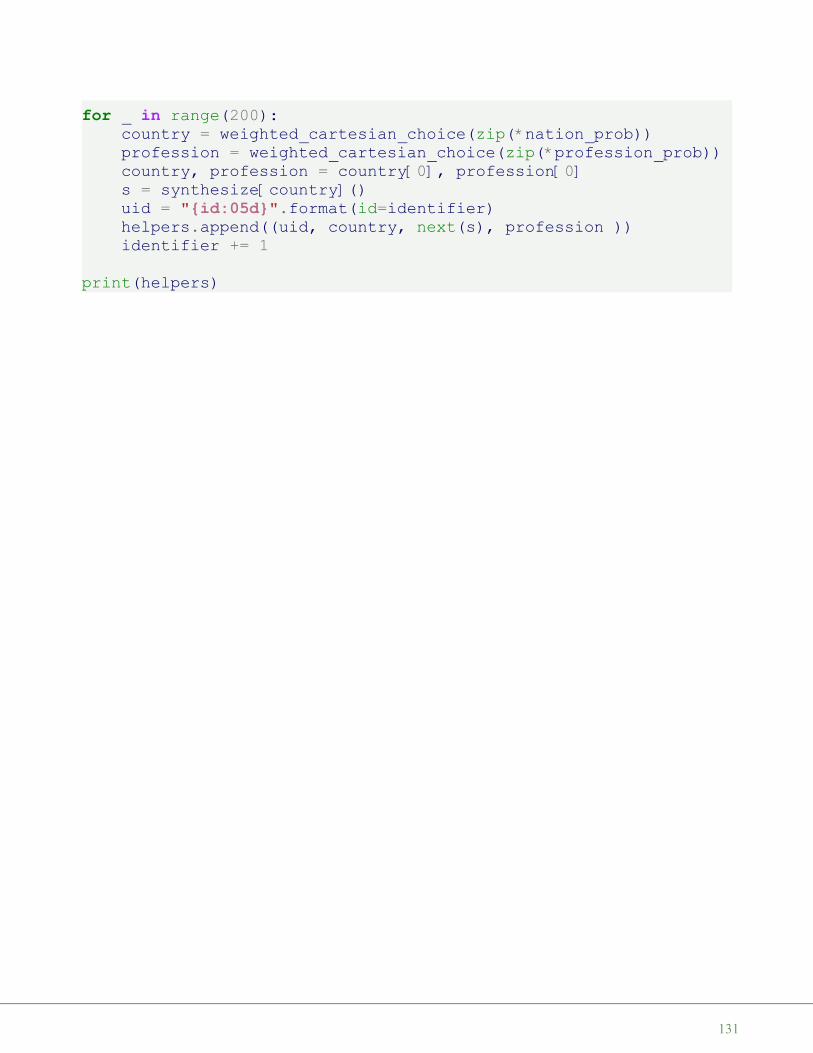
for _ in range(200):country = weighted_cartesian_choice(zip(*nation_prob))profession = weighted_cartesian_choice(zip(*profession_prob))country, profession = country[0], profession[0]s = synthesize[country]()uid = "{id:05d}".format(id=identifier)helpers.append((uid, country, next(s), profession ))identifier += 1

print(helpers)

131

[('00001', 'Germany', 'Brigitte Wagner', 'Social Worker'), ('00002', 'France', 'Chloé Muller', 'Medical Aid'), ('00003', 'Switzerland', 'Laura Steiner', 'Medical Aid'), ('00004', 'France', 'Laura Matin', 'Medical Aid'), ('00005', 'France', 'Léa Fontaine', 'Social Worker'), ('00006', 'Switzerland', 'Océane Meyer', 'Social Worker'), ('00007', 'France', 'Léa Fournier', 'Social Worker'), ('00008', 'France', 'Marie Matin', 'Social Worker'), ('00009', 'France', 'Laura Durand', 'Security Aid'), ('00010', 'France', 'Maxime Dubois', 'Social Worker'), ('00011', 'France', 'Nicolas Mercier','Social Worker'), ('00012', 'Italy', 'Mattia Gallo', 'Medical Aid'), ('00013', 'France', 'Quentin Leroy', 'Social Worker'), ('00014', 'Germany', 'Wolfgang Koch', 'Medical Aid'), ('00015', 'France', 'Manon Matin', 'Social Worker'), ('00016', 'Switzerland', 'Mélissa Schneider', 'Social Worker'), ('00017', 'Germany', 'Thomas Koch', 'Social Worker'), ('00018', 'Germany', 'Wolfgang Schäfer', 'Medical Aid'), ('00019', 'Germany', 'Peter Schäfer', 'Security Aid'), ('00020', 'Italy', 'Alice Costa', 'Medical Aid'), ('00021','Switzerland', 'Océane Steiner', 'Social Worker'), ('00022', 'France', 'Manon Durand', 'Medical Aid'), ('00023', 'Switzerland', 'Daniel Meier', 'Social Worker'), ('00024', 'France', 'Laura Fournier', 'Social Worker'), ('00025', 'Switzerland', 'Daniel Schneider', 'Security Aid'), ('00026', 'Germany', 'Maria Weber', 'Social Worker'), ('00027', 'Switzerland', 'Sarah Weber', 'Medical Aid'),('00028', 'Germany', 'Wolfgang Weber', 'Social Worker'), ('00029', 'Germany', 'Michael Fischer', 'Social Worker'), ('00030', 'Germany', 'Stefanie Hoffmann', 'Social Worker'), ('00031', 'France','Laura Mercier', 'Social Worker'), ('00032', 'France', 'Nicolas Leroy', 'Social Worker'), ('00033', 'Germany', 'Peter Becker', 'Social Worker'), ('00034', 'France', 'Maxime Petit', 'Social Worker'), ('00035', 'France', 'Maxime Matin', 'Security Aid'), ('00036', 'Germany', 'Stefanie Becker', 'Medical Aid'), ('00037', 'France', 'Laura Petit', 'Social Worker'), ('00038', 'Switzerland', 'Hans Fischer', 'Social Worker'), ('00039', 'France', 'Nicolas Leroy', 'Medical Aid'), ('00040', 'France', 'Léa Matin', 'Social Worker'), ('00041', 'Switzerland', 'Bruno Fischer', 'Social Worker'),('00042', 'France', 'Julien Dubois', 'Medical Aid'), ('00043', 'France', 'Alexandre Petit', 'Social Worker'), ('00044', 'France', 'Camille Camille', 'Social Worker'), ('00045', 'France', 'Camille Rousseau', 'Medical Aid'), ('00046', 'France', 'Julien Lambert', 'Social Worker'), ('00047', 'France', 'Léa Dubois', 'Social Worker'), ('00048', 'Italy', 'Lorenzo Mancini', 'Security Aid'), ('00049', 'Germany', 'Ursula Hoffmann', 'Social Worker'), ('00050', 'Germany', 'Brigitte Meyer', 'Medical Aid'), ('00051', 'France', 'Sandra Lambert', 'Social Worker'), ('00052', 'Italy', 'Alice Rizzo','Medical Aid'), ('00053', 'France', 'Chloé Nicolas', 'Social Worker'), ('00054', 'Germany', 'Gabriele Schröder', 'Social Worker'),

132

('00055', 'France', 'Thomas Durand', 'Medical Aid'), ('00056', 'France', 'Léa Dubois', 'Medical Aid'), ('00057', 'France', 'Maxime Mercier', 'Social Worker'), ('00058', 'Germany', 'Peter Schmidt','Social Worker'), ('00059', 'France', 'Quentin Durand', 'Social Worker'), ('00060', 'France', 'Camille Petit', 'Social Worker'), ('00061', 'Switzerland', 'Laura Schmid', 'Medical Aid'), ('00062', 'Italy', 'Gabriele Lombardi', 'Social Worker'), ('00063', 'Switzerland', 'Peter Meier', 'Medical Aid'), ('00064', 'Switzerland', 'Reto Huber', 'Medical Aid'), ('00065', 'Italy', 'Matteo Mancini', 'Medical Aid'), ('00066', 'France', 'Marie Petit', 'Social Worker'),('00067', 'Germany', 'Manfred Hoffmann', 'Medical Aid'), ('00068', 'Germany', 'Brigitte Schmidt', 'Medical Aid'), ('00069', 'France', 'Manon Matin', 'Medical Aid'), ('00070', 'France', 'Nicolas Petit', 'Social Worker'), ('00071', 'France', 'Léa Petit', 'SocialWorker'), ('00072', 'Germany', 'Monika Schulz', 'Social Worker'),('00073', 'Italy', 'Mattia Rizzo', 'Social Worker'), ('00074', 'Italy', 'Sofia Colombo', 'Social Worker'), ('00075', 'Germany', 'Michael Schäfer', 'Medical Aid'), ('00076', 'Germany', 'Matthias Hoffmann', 'Social Worker'), ('00077', 'Germany', 'Wolfgang Schneider', 'Social Worker'), ('00078', 'France', 'Julien Dubois', 'Social Worker'), ('00079', 'Germany', 'Peter Fischer', 'Social Worker'), ('00080', 'France', 'Julien Leroy', 'Social Worker'), ('00081', 'France', 'Julien Bernard', 'Social Worker'), ('00082', 'Germany', 'Michael Schmidt', 'Social Worker'), ('00083', 'France', 'Manon Bernard', 'Social Worker'), ('00084', 'Switzerland', 'Hans Huber', 'Security Aid'), ('00085', 'Germany', 'Monika Schneider', 'Medical Aid'), ('00086', 'Switzerland', 'Noémie Müller', 'Security Aid'), ('00087', 'Switzerland', 'Sarah Gerber', 'Medical Aid'), ('00088', 'Germany', 'Thomas Müller', 'Medical Aid'), ('00089', 'Switzerland', 'Sarah Weber', 'Medical Aid'), ('00090', 'France', 'Laura Petit', 'Medical Aid'), ('00091', 'Switzerland', 'Sarah Gerber', 'Medical Aid'), ('00092', 'Switzerland', 'Reto Schmid', 'Medical Aid'), ('00093', 'Germany', 'Monika Schneider', 'Medical Aid'), ('00094', 'France', 'Quentin Matin', 'Social Worker'), ('00095', 'Italy', 'Aurora Colombo', 'Social Worker'), ('00096', 'Germany', 'Ursula Meyer', 'Social Worker'), ('00097', 'Germany', 'Manfred Weber', 'Social Worker'), ('00098', 'Italy', 'Giulia Ferrari','Medical Aid'), ('00099', 'France', 'Thomas Muller', 'Social Worker'), ('00100', 'Switzerland', 'Daniel Schneider', 'Medical Aid'),('00101', 'France', 'Maxime Camille', 'Medical Aid'), ('00102', 'France', 'Laura Petit', 'Social Worker'), ('00103', 'Germany', 'Manfred Schmidt', 'Medical Aid'), ('00104', 'Italy', 'Martina Lombardi', 'Social Worker'), ('00105', 'Switzerland', 'Sarah Baumann', 'Medical Aid'), ('00106', 'Switzerland', 'Bruno Gerber', 'Security Aid'), ('00107', 'Switzerland', 'Laura Müller', 'Social Worker'),('00108', 'Germany', 'Andreas Weber', 'Social Worker'), ('00109',

133

'Switzerland', 'Hans Fischer', 'Social Worker'), ('00110', 'Switzerland', 'Daniel Meyer', 'Social Worker'), ('00111', 'France', 'Julien Rousseau', 'Security Aid'), ('00112', 'Switzerland', 'Reto Schmid', 'Social Worker'), ('00113', 'Switzerland', 'Urli Schneider', 'Social Worker'), ('00114', 'France', 'Grégory Rousseau', 'Medical Aid'), ('00115', 'France', 'Marie Durand', 'Social Worker'),('00116', 'France', 'Léa Durand', 'Social Worker'), ('00117', 'France', 'Camille Matin', 'Medical Aid'), ('00118', 'Germany', 'Wolfgang Schneider', 'Social Worker'), ('00119', 'France', 'Julien Matin', 'Social Worker'), ('00120', 'France', 'Marie Leroy', 'Social Worker'), ('00121', 'Switzerland', 'Mélissa Brunner', 'Security Aid'), ('00122', 'Germany', 'Ursula Schneider', 'Social Worker'),('00123', 'France', 'Camille Mercier', 'Social Worker'), ('00124', 'France', 'Julien Camille', 'Social Worker'), ('00125', 'Switzerland', 'Laura Schmid', 'Medical Aid'), ('00126', 'France', 'Camille Durand', 'Social Worker'), ('00127', 'France', 'Marie Camille', 'Medical Aid'), ('00128', 'Germany', 'Monika Wagner', 'SocialWorker'), ('00129', 'Italy', 'Giorgia Esposito', 'Security Aid'),('00130', 'France', 'Clementine Mercier', 'Social Worker'), ('00131', 'France', 'Marie Matin', 'Social Worker'), ('00132', 'Switzerland', 'Noémie Brunner', 'Medical Aid'), ('00133', 'France', 'Nicolas Leroy', 'Security Aid'), ('00134', 'France', 'Camille Camille', 'Social Worker'), ('00135', 'Germany', 'Wolfgang Fischer', 'Medical Aid'), ('00136', 'Germany', 'Brigitte Müller', 'Medical Aid'), ('00137', 'Germany', 'Peter Schneider', 'Social Worker'), ('00138', 'Switzerland', 'Laura Schneider', 'Medical Aid'), ('00139', 'France', 'Chloé Rousseau', 'Social Worker'), ('00140', 'Italy', 'Alice De Luca', 'Medical Aid'), ('00141', 'France', 'Thomas Bernard', 'Social Worker'), ('00142', 'Italy', 'Francesco Grecco','Medical Aid'), ('00143', 'Switzerland', 'Peter Frei', 'Medical Aid'), ('00144', 'France', 'Philippe Mercier', 'Security Aid'), ('00145', 'Germany', 'Monika Meyer', 'Social Worker'), ('00146', 'France', 'Alexandre Lambert', 'Medical Aid'), ('00147', 'Switzerland', 'Sarah Brunner', 'Security Aid'), ('00148', 'Germany', 'Wolfgang Schneider', 'Social Worker'), ('00149', 'Germany', 'Manfred Müller', 'Social Worker'), ('00150', 'France', 'Léa Dubois', 'Medical Aid'), ('00151', 'Switzerland', 'Reto Schmid', 'Medical Aid'),('00152', 'France', 'Manon Lambert', 'Social Worker'), ('00153','France', 'Chloé Fournier', 'Social Worker'), ('00154', 'France','Grégory Bernard', 'Social Worker'), ('00155', 'Italy', 'Martina Bruno', 'Social Worker'), ('00156', 'France', 'Marie Nicolas', 'Social Worker'), ('00157', 'Italy', 'Giorgia Romano', 'Social Worker'), ('00158', 'France', 'Thomas Mercier', 'Security Aid'), ('00159', 'Germany', 'Manfred Richter', 'Social Worker'), ('00160', 'Germany', 'Wolfgang Schäfer', 'Social Worker'), ('00161', 'Germany','Peter Müller', 'Security Aid'), ('00162', 'Switzerland', 'Océane

134

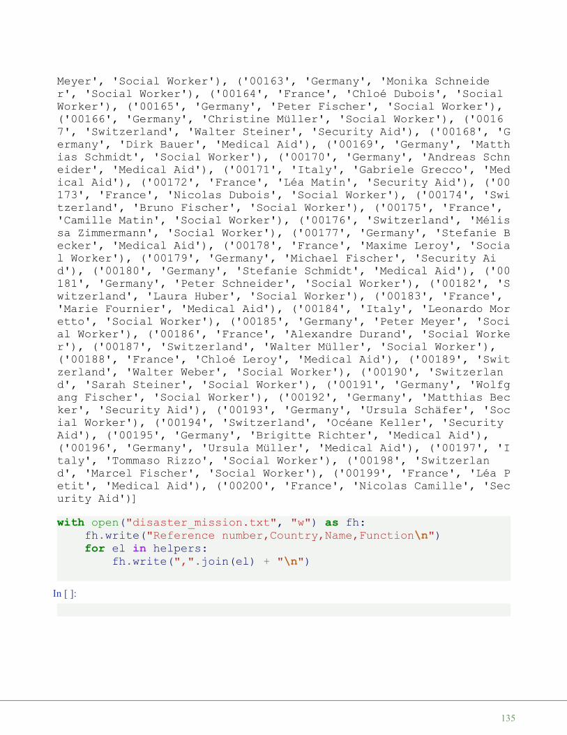
with open("disaster_mission.txt", "w") as fh:fh.write("Reference number,Country,Name,Function\n")for el in helpers:

fh.write(",".join(el) + "\n")

In [ ]:

Meyer', 'Social Worker'), ('00163', 'Germany', 'Monika Schneider', 'Social Worker'), ('00164', 'France', 'Chloé Dubois', 'SocialWorker'), ('00165', 'Germany', 'Peter Fischer', 'Social Worker'),('00166', 'Germany', 'Christine Müller', 'Social Worker'), ('00167', 'Switzerland', 'Walter Steiner', 'Security Aid'), ('00168', 'Germany', 'Dirk Bauer', 'Medical Aid'), ('00169', 'Germany', 'Matthias Schmidt', 'Social Worker'), ('00170', 'Germany', 'Andreas Schneider', 'Medical Aid'), ('00171', 'Italy', 'Gabriele Grecco', 'Medical Aid'), ('00172', 'France', 'Léa Matin', 'Security Aid'), ('00173', 'France', 'Nicolas Dubois', 'Social Worker'), ('00174', 'Switzerland', 'Bruno Fischer', 'Social Worker'), ('00175', 'France','Camille Matin', 'Social Worker'), ('00176', 'Switzerland', 'Mélissa Zimmermann', 'Social Worker'), ('00177', 'Germany', 'Stefanie Becker', 'Medical Aid'), ('00178', 'France', 'Maxime Leroy', 'Social Worker'), ('00179', 'Germany', 'Michael Fischer', 'Security Aid'), ('00180', 'Germany', 'Stefanie Schmidt', 'Medical Aid'), ('00181', 'Germany', 'Peter Schneider', 'Social Worker'), ('00182', 'Switzerland', 'Laura Huber', 'Social Worker'), ('00183', 'France','Marie Fournier', 'Medical Aid'), ('00184', 'Italy', 'Leonardo Moretto', 'Social Worker'), ('00185', 'Germany', 'Peter Meyer', 'Social Worker'), ('00186', 'France', 'Alexandre Durand', 'Social Worker'), ('00187', 'Switzerland', 'Walter Müller', 'Social Worker'),('00188', 'France', 'Chloé Leroy', 'Medical Aid'), ('00189', 'Switzerland', 'Walter Weber', 'Social Worker'), ('00190', 'Switzerland', 'Sarah Steiner', 'Social Worker'), ('00191', 'Germany', 'Wolfgang Fischer', 'Social Worker'), ('00192', 'Germany', 'Matthias Becker', 'Security Aid'), ('00193', 'Germany', 'Ursula Schäfer', 'Social Worker'), ('00194', 'Switzerland', 'Océane Keller', 'SecurityAid'), ('00195', 'Germany', 'Brigitte Richter', 'Medical Aid'),('00196', 'Germany', 'Ursula Müller', 'Medical Aid'), ('00197', 'Italy', 'Tommaso Rizzo', 'Social Worker'), ('00198', 'Switzerland', 'Marcel Fischer', 'Social Worker'), ('00199', 'France', 'Léa Petit', 'Medical Aid'), ('00200', 'France', 'Nicolas Camille', 'Security Aid')]

135

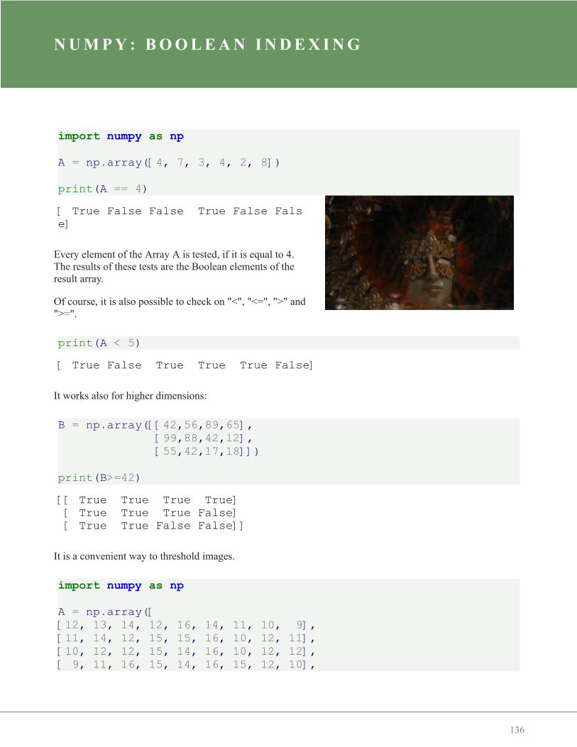
N U M P Y : B O O L E A N I N D E X I N G

import numpy as npA = np.array([4, 7, 3, 4, 2, 8])

print(A == 4)

Every element of the Array A is tested, if it is equal to 4.The results of these tests are the Boolean elements of theresult array.

Of course, it is also possible to check on "<", "<=", ">" and">=".

print(A < 5)

It works also for higher dimensions:

B = np.array([[42,56,89,65],[99,88,42,12],[55,42,17,18]])

print(B>=42)

It is a convenient way to threshold images.

import numpy as npA = np.array([[12, 13, 14, 12, 16, 14, 11, 10, 9],[11, 14, 12, 15, 15, 16, 10, 12, 11],[10, 12, 12, 15, 14, 16, 10, 12, 12],[ 9, 11, 16, 15, 14, 16, 15, 12, 10],

[ True False False True False False]

[ True False True True True False]

[[ True True True True][ True True True False][ True True False False]]

136

[12, 11, 16, 14, 10, 12, 16, 12, 13],[10, 15, 16, 14, 14, 14, 16, 15, 12],[13, 17, 14, 10, 14, 11, 14, 15, 10],[10, 16, 12, 14, 11, 12, 14, 18, 11],[10, 19, 12, 14, 11, 12, 14, 18, 10],[14, 22, 17, 19, 16, 17, 18, 17, 13],[10, 16, 12, 14, 11, 12, 14, 18, 11],[10, 16, 12, 14, 11, 12, 14, 18, 11],[10, 19, 12, 14, 11, 12, 14, 18, 10],[14, 22, 12, 14, 11, 12, 14, 17, 13],[10, 16, 12, 14, 11, 12, 14, 18, 11]])

B = A < 15B.astype(np.int)

If you have a close look at the previous output, you will see, that it the upper case 'A' is hidden in the array B.

FANCY INDEXING

We will index an array C in the following example by using a Boolean mask. It is called fancy indexing, ifarrays are indexed by using boolean or integer arrays (masks). The result will be a copy and not a view.

In our next example, we will use the Boolean mask of one array to select the corresponding elements ofanother array. The new array R contains all the elements of C where the corresponding value of (A<=5) isTrue.

Output: array([[1, 1, 1, 1, 0, 1, 1, 1, 1],[1, 1, 1, 0, 0, 0, 1, 1, 1],[1, 1, 1, 0, 1, 0, 1, 1, 1],[1, 1, 0, 0, 1, 0, 0, 1, 1],[1, 1, 0, 1, 1, 1, 0, 1, 1],[1, 0, 0, 1, 1, 1, 0, 0, 1],[1, 0, 1, 1, 1, 1, 1, 0, 1],[1, 0, 1, 1, 1, 1, 1, 0, 1],[1, 0, 1, 1, 1, 1, 1, 0, 1],[1, 0, 0, 0, 0, 0, 0, 0, 1],[1, 0, 1, 1, 1, 1, 1, 0, 1],[1, 0, 1, 1, 1, 1, 1, 0, 1],[1, 0, 1, 1, 1, 1, 1, 0, 1],[1, 0, 1, 1, 1, 1, 1, 0, 1],[1, 0, 1, 1, 1, 1, 1, 0, 1]])

137

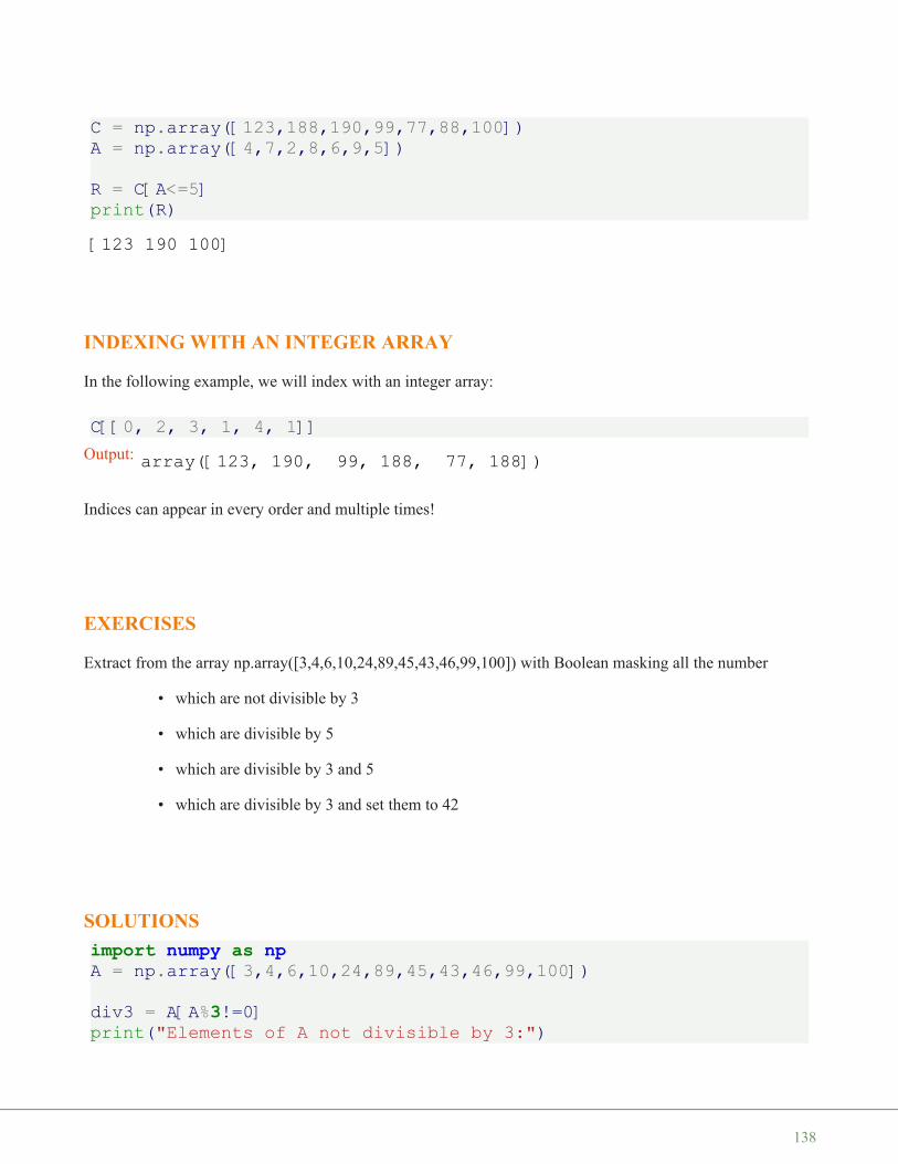
C = np.array([123,188,190,99,77,88,100])A = np.array([4,7,2,8,6,9,5])

R = C[A<=5]print(R)

INDEXING WITH AN INTEGER ARRAY

In the following example, we will index with an integer array:

C[[0, 2, 3, 1, 4, 1]]

Indices can appear in every order and multiple times!

EXERCISES

Extract from the array np.array([3,4,6,10,24,89,45,43,46,99,100]) with Boolean masking all the number

• which are not divisible by 3

• which are divisible by 5

• which are divisible by 3 and 5

• which are divisible by 3 and set them to 42

SOLUTIONSimport numpy as npA = np.array([3,4,6,10,24,89,45,43,46,99,100])

div3 = A[A%3!=0]print("Elements of A not divisible by 3:")

[123 190 100]

Output: array([123, 190, 99, 188, 77, 188])

138

print(div3)

div5 = A[A%5==0]print("Elements of A divisible by 5:")print(div5)

print("Elements of A, which are divisible by 3 and 5:")print(A[(A%3==0) & (A%5==0)])print("------------------")

#

A[A%3==0] = 42print("""New values of A after setting the elements of A,which are divisible by 3, to 42:""")print(A)

NONZERO AND WHERE

There is an ndarray method called nonzero and a numpy method with this name. The two functions areequivalent.

For an ndarray a both numpy.nonzero(a) and a.nonzero() return the indices of the elements of a that are non-zero. The indices are returned as a tuple of arrays, one for each dimension of 'a'. The corresponding non-zerovalues can be obtained with:

a[numpy.nonzero(a)]

import numpy as npa = np.array([[0, 2, 3, 0, 1],

Elements of A not divisible by 3:[ 4 10 89 43 46 100]Elements of A divisible by 5:[ 10 45 100]Elements of A, which are divisible by 3 and 5:[45]------------------New values of A after setting the elements of A,which are divisible by 3, to 42:[ 42 4 42 10 42 89 42 43 46 42 100]

139

[1, 0, 0, 7, 0],[5, 0, 0, 1, 0]])

print(a.nonzero())

If you want to group the indices by element, you can use transpose:

transpose(nonzero(a))

A two-dimensional array is returned. Every row corresponds to a non-zero element.

np.transpose(a.nonzero())

The corresponding non-zero values can be retrieved with:

a[a.nonzero()]

The function 'nonzero' can be used to obtain the indices of an array, where a condition is True. In the followingscript, we create the Boolean array B >= 42:

B = np.array([[42,56,89,65],[99,88,42,12],[55,42,17,18]])

print(B >= 42)

np.nonzero(B >= 42) yields the indices of the B where the condition is true:

(array([0, 0, 0, 1, 1, 2, 2]), array([1, 2, 4, 0, 3, 0, 3]))

Output: array([[0, 1],[0, 2],[0, 4],[1, 0],[1, 3],[2, 0],[2, 3]])

Output: array([2, 3, 1, 1, 7, 5, 1])

[[ True True True True][ True True True False][ True True False False]]

140

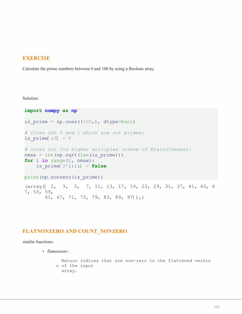
EXERCISE

Calculate the prime numbers between 0 and 100 by using a Boolean array.

Solution:

import numpy as npis_prime = np.ones((100,), dtype=bool)

# Cross out 0 and 1 which are not primes:is_prime[:2] = 0

# cross out its higher multiples (sieve of Eratosthenes):nmax = int(np.sqrt(len(is_prime)))for i in range(2, nmax):

is_prime[2*i::i] = Falseprint(np.nonzero(is_prime))

FLATNONZERO AND COUNT_NONZERO

similar functions:

• flatnonzero :

Return indices that are non-zero in the flattened version of the input

array.

(array([ 2, 3, 5, 7, 11, 13, 17, 19, 23, 29, 31, 37, 41, 43, 47, 53, 59,

61, 67, 71, 73, 79, 83, 89, 97]),)

141

• count_nonzero :

Counts the number of non-zero elements in the input array.

142

M A T R I X M U L T I P L I C A I O N , D O T A N D C R O S SP R O D U C T

Distorted Abacus In the previous chapter of our introduction in NumPy wehave demonstrated how to create and change Arrays. In this chapter wewant to show, how we can perform in Python with the module NumPy allthe basic Matrix Arithmetics like

• Matrix addition• Matrix subtraction• Matrix multiplication• Scalar product• Cross product• and lots of other operations on matrices

The arithemtic standard Operators

• +• -• *• /

• %

are applied on the elements, this means that the arrays have to have the same size.

import numpy as npx = np.array([1, 5, 2])y = np.array([7, 4, 1])x + y

x * y

In [ ]:

x - yx / y

Output: array([8, 9, 3])

Output: array([ 7, 20, 2])

Output: array([0.14285714, 1.25 , 2. ])

143

x % y

VECTOR ADDITION AND SUBTRACTION

Many people know vector additionand subtraction from physics, to beexact from the parallelogram offorces. It is a method for solving(or visualizing) the results ofapplying two forces to an object.

The addition of two vectors, in ourexample (see picture) x and y, maybe represented graphically byplacing the start of the arrow y atthe tip of the arrow x, and thendrawing an arrow from the start (tail) of x to the tip (head) of y. The new arrow drawn represents the vector x+ y

x = np.array([3, 2])y = np.array([5, 1])z = x + yz

Subtracting a vector is the same as addingits negative. So, the difference of thevectors x and y is equal to the sum of x and-y: x - y = x + (-y) Subtraction of twovectors can be geometrically defined asfollows: to subtract y from x, we place theend points of x and y at the same point,and then draw an arrow from the tip of y tothe tip of x. That arrow represents thevector x - y, see picture on the right side.

Mathematically, we subtract the corresponding components of vector y from the vector x.

SCALAR PRODUCT / DOT PRODUCT

In mathematics, the dot product is an algebraic operation that takes two coordinate vectors of equal size andreturns a single number. The result is calculated by multiplying corresponding entries and adding up those

Output: array([1, 1, 0])

Output: array([8, 3])

144

products. The name "dot product" stems from the fact that the centered dot "·" is often used to designate thisoperation. The name "scalar product" focusses on the scalar nature of the result. of the result.

Definition of the scalar product:

We can see from the definition of the scalar product that it can be used to calculate the cosine of the anglebetween two vectors.

Calculation of the scalar product:

Finally, we want to demonstrate how to calculate the scalar product in Python:

x = np.array([1, 2, 3])y = np.array([-7, 8, 9])np.dot(x, y)

dot = np.dot(x ,y)x_modulus = np.sqrt((x*x).sum())y_modulus = np.sqrt((y*y).sum())cos_angle = dot / x_modulus / y_modulus # cosine of angle betweenx and yangle = np.arccos(cos_angle)angle

angle * 360 / 2 / np.pi # angle in degrees

In [ ]:

36>>> dot = np.dot(x,y)>>> x_modulus = np.sqrt((x*x).sum())>>> y_modulus = np.sqrt((y*y).sum())>>> cos_angle = dot / x_modulus / y_modulus # cosine of angle betw

Output: 36

Output: 0.808233789010825

Output: 46.308384970187326

145

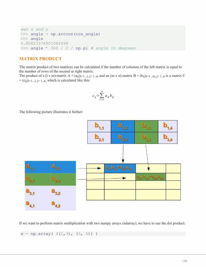
een x and y>>> angle = np.arccos(cos_angle)>>> angle0.80823378901082499>>> angle * 360 / 2 / np.pi # angle in degrees

MATRIX PRODUCT

The matrix product of two matrices can be calculated if the number of columns of the left matrix is equal tothe number of rows of the second or right matrix.The product of a (l x m)-matrix A = (aij)i=1...l, j= 1..m and an (m x n)-matrix B = (bij)i=1...m, j= 1..n is a matrix C= (cij)i=1...l, j= 1..n, which is calculated like this:

The following picture illustrates it further:

If we want to perform matrix multiplication with two numpy arrays (ndarray), we have to use the dot product:

x = np.array( ((2,3), (3, 5)) )

146

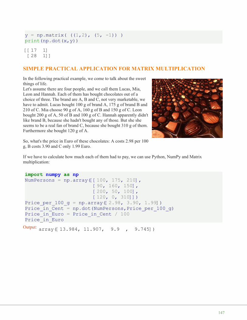
y = np.matrix( ((1,2), (5, -1)) )print(np.dot(x,y))

SIMPLE PRACTICAL APPLICATION FOR MATRIX MULTIPLICATION

In the following practical example, we come to talk about the sweetthings of life.Let's assume there are four people, and we call them Lucas, Mia,Leon and Hannah. Each of them has bought chocolates out of achoice of three. The brand are A, B and C, not very marketable, wehave to admit. Lucas bought 100 g of brand A, 175 g of brand B and210 of C. Mia choose 90 g of A, 160 g of B and 150 g of C. Leonbought 200 g of A, 50 of B and 100 g of C. Hannah apparently didn'tlike brand B, because she hadn't bought any of those. But she sheseems to be a real fan of brand C, because she bought 310 g of them.Furthermore she bought 120 g of A.

So, what's the price in Euro of these chocolates: A costs 2.98 per 100g, B costs 3.90 and C only 1.99 Euro.

If we have to calculate how much each of them had to pay, we can use Python, NumPy and Matrixmultiplication:

import numpy as npNumPersons = np.array([[100, 175, 210],

[90, 160, 150],[200, 50, 100],[120, 0, 310]])

Price_per_100_g = np.array([2.98, 3.90, 1.99])Price_in_Cent = np.dot(NumPersons,Price_per_100_g)Price_in_Euro = Price_in_Cent / 100Price_in_Euro

[[17 1][28 1]]

Output: array([13.984, 11.907, 9.9 , 9.745])

147

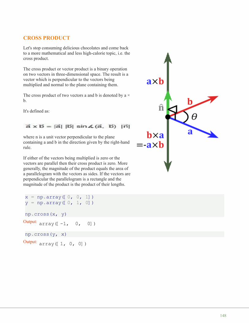
CROSS PRODUCT

Let's stop consuming delicious chocolates and come backto a more mathematical and less high-calorie topic, i.e. thecross product.

The cross product or vector product is a binary operationon two vectors in three-dimensional space. The result is avector which is perpendicular to the vectors beingmultiplied and normal to the plane containing them.

The cross product of two vectors a and b is denoted by a ×b.

It's defined as:

where n is a unit vector perpendicular to the planecontaining a and b in the direction given by the right-handrule.

If either of the vectors being multiplied is zero or thevectors are parallel then their cross product is zero. Moregenerally, the magnitude of the product equals the area ofa parallelogram with the vectors as sides. If the vectors areperpendicular the parallelogram is a rectangle and themagnitude of the product is the product of their lengths.

x = np.array([0, 0, 1])y = np.array([0, 1, 0])

np.cross(x, y)

np.cross(y, x)

Output: array([-1, 0, 0])

Output: array([1, 0, 0])

148

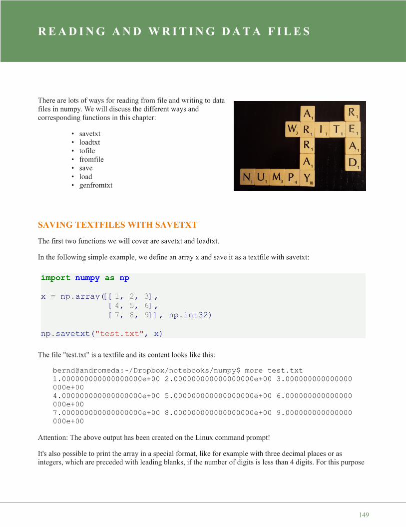
R E A D I N G A N D W R I T I N G D A T A F I L E S

There are lots of ways for reading from file and writing to datafiles in numpy. We will discuss the different ways andcorresponding functions in this chapter:

• savetxt• loadtxt• tofile• fromfile• save• load• genfromtxt

SAVING TEXTFILES WITH SAVETXT

The first two functions we will cover are savetxt and loadtxt.

In the following simple example, we define an array x and save it as a textfile with savetxt:

import numpy as npx = np.array([[1, 2, 3],

[4, 5, 6],[7, 8, 9]], np.int32)

np.savetxt("test.txt", x)

The file "test.txt" is a textfile and its content looks like this:

bernd@andromeda:~/Dropbox/notebooks/numpy$ more test.txt1.000000000000000000e+00 2.000000000000000000e+00 3.000000000000000000e+004.000000000000000000e+00 5.000000000000000000e+00 6.000000000000000000e+007.000000000000000000e+00 8.000000000000000000e+00 9.000000000000000000e+00

Attention: The above output has been created on the Linux command prompt!

It's also possible to print the array in a special format, like for example with three decimal places or asintegers, which are preceded with leading blanks, if the number of digits is less than 4 digits. For this purpose

149

we assign a format string to the third parameter 'fmt'. We saw in our first example that the default delimeter isa blank. We can change this behaviour by assigning a string to the parameter "delimiter". In most cases thisstring will consist solely of a single character but it can be a sequence of character, like a smiley " :-) " as well:

np.savetxt("test2.txt", x, fmt="%2.3f", delimiter=",")np.savetxt("test3.txt", x, fmt="%04d", delimiter=" :-) ")

The newly created files look like this:

bernd@andromeda:~/Dropbox/notebooks/numpy$ more test2.txt1.000,2.000,3.0004.000,5.000,6.0007.000,8.000,9.000bernd@andromeda:~/Dropbox/notebooks/numpy$ more test3.txt0001 :-) 0002 :-) 00030004 :-) 0005 :-) 00060007 :-) 0008 :-) 0009

The complete syntax of savetxt looks like this:

savetxt(fname, X, fmt='%.18e', delimiter=' ', newline='\n', header='', footer='', comments='# ')

Parameter Meaning

X array_like Data to be saved to a text file.

fmt

str or sequence of strs, optionalA single format (%10.5f), a sequence of formats, or a multi-format string, e.g. 'Iteration %d -- %10.5f', in which

case 'delimiter' is ignored. For complex 'X', the legal options for 'fmt' are:a) a single specifier, "fmt='%.4e'", resulting in numbers formatted like "' (%s+%sj)' % (fmt, fmt)"

b) a full string specifying every real and imaginary part, e.g. "' %.4e %+.4j %.4e %+.4j %.4e %+.4j'" for 3 columnsc) a list of specifiers, one per column - in this case, the real and imaginary part must have separate specifiers, e.g.

"['%.3e + %.3ej', '(%.15e%+.15ej)']" for 2 columns

delimiter A string used for separating the columns.

newline A string (e.g. "\n", "\r\n" or ",\n") which will end a line instead of the default line ending

header A String that will be written at the beginning of the file.

footer A String that will be written at the end of the file.

comments A String that will be prepended to the 'header' and 'footer' strings, to mark them as comments. The hash tag '#' is

150

Parameter Meaning

used as the default.

LOADING TEXTFILES WITH LOADTXT

We will read in now the file "test.txt", which we have written in our previous subchapter:

y = np.loadtxt("test.txt")print(y)

y = np.loadtxt("test2.txt", delimiter=",")print(y)

Nothing new, if we read in our text, in which we used a smiley to separator:

y = np.loadtxt("test3.txt", delimiter=" :-) ")print(y)

It's also possible to choose the columns by index:

y = np.loadtxt("test3.txt", delimiter=" :-) ", usecols=(0,2))print(y)

[[ 1. 2. 3.][ 4. 5. 6.][ 7. 8. 9.]]

[[ 1. 2. 3.][ 4. 5. 6.][ 7. 8. 9.]]

[[ 1. 2. 3.][ 4. 5. 6.][ 7. 8. 9.]]

[[ 1. 3.][ 4. 6.][ 7. 9.]]

151

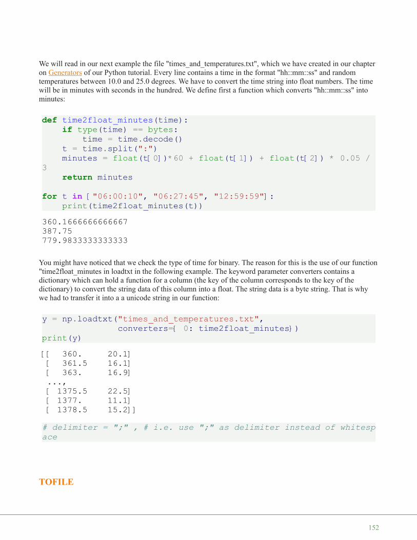
We will read in our next example the file "times_and_temperatures.txt", which we have created in our chapteron Generators of our Python tutorial. Every line contains a time in the format "hh::mm::ss" and randomtemperatures between 10.0 and 25.0 degrees. We have to convert the time string into float numbers. The timewill be in minutes with seconds in the hundred. We define first a function which converts "hh::mm::ss" intominutes:

def time2float_minutes(time):if type(time) == bytes:

time = time.decode()t = time.split(":")minutes = float(t[0])*60 + float(t[1]) + float(t[2]) * 0.05 /

3return minutes

for t in ["06:00:10", "06:27:45", "12:59:59"]:print(time2float_minutes(t))

You might have noticed that we check the type of time for binary. The reason for this is the use of our function"time2float_minutes in loadtxt in the following example. The keyword parameter converters contains adictionary which can hold a function for a column (the key of the column corresponds to the key of thedictionary) to convert the string data of this column into a float. The string data is a byte string. That is whywe had to transfer it into a a unicode string in our function:

y = np.loadtxt("times_and_temperatures.txt",converters={ 0: time2float_minutes})

print(y)

# delimiter = ";" , # i.e. use ";" as delimiter instead of whitespace

TOFILE

360.1666666666667387.75779.9833333333333

[[ 360. 20.1][ 361.5 16.1][ 363. 16.9]...,[ 1375.5 22.5][ 1377. 11.1][ 1378.5 15.2]]

152

tofile is a function to write the content of an array to a file both in binary, which is the default, and text format.

A.tofile(fid, sep="", format="%s")

The data of the A ndarry is always written in 'C' order, regardless of the order of A.

The data file written by this method can be reloaded with the function fromfile() .

Parameter Meaning

fid can be either an open file object, or a string containing a filename.

sepThe string 'sep' defines the separator between array items for text output. If it is empty (''), a binary file is written,

equivalent to file.write(a.tostring()).

formatFormat string for text file output. Each entry in the array is formatted to text by first converting it to the closest

Python type, and then using 'format' % item.

Remark:

Information on endianness and precision is lost. Therefore it may not be a good idea to use the function toarchive data or transport data between machines with different endianness. Some of these problems can beovercome by outputting the data as text files, at the expense of speed and file size.

dt = np.dtype([('time', [('min', int), ('sec', int)]),('temp', float)])

x = np.zeros((1,), dtype=dt)x['time']['min'] = 10x['temp'] = 98.25print(x)

fh = open("test6.txt", "bw")x.tofile(fh)

FROMFILE

fromfile to read in data, which has been written with the tofile function. It's possible to read binarydata, if the data type is known. It's also possible to parse simply formatted text files. The data from the file isturned into an array.

[((10, 0), 98.25)]

153

The general syntax looks like this:

numpy.fromfile(file, dtype=float, count=-1, sep='')

Parameter Meaning

file 'file' can be either a file object or the name of the file to read.

dtypedefines the data type of the array, which will be constructed from the file data. For binary files, it is used to

determine the size and byte-order of the items in the file.

count defines the number of items, which will be read. -1 means all items will be read.

sepThe string 'sep' defines the separator between the items, if the file is a text file. If it is empty (''), the file will be

treated as a binary file. A space (" ") in a separator matches zero or more whitespace characters. A separatorconsisting solely of spaces has to match at least one whitespace.

fh = open("test4.txt", "rb")

np.fromfile(fh, dtype=dt)

import numpy as npimport os# platform dependent: difference between Linux and Windows#data = np.arange(50, dtype=np.int)

data = np.arange(50, dtype=np.int32)data.tofile("test4.txt")

fh = open("test4.txt", "rb")# 4 * 32 = 128fh.seek(128, os.SEEK_SET)

Output: array([((4294967296, 12884901890), 1.0609978957e-313),((30064771078, 38654705672), 2.33419537056e-313),((55834574860, 64424509454), 3.60739284543e-313),((81604378642, 90194313236), 4.8805903203e-313),((107374182424, 115964117018), 6.1537877952e-313),((133143986206, 141733920800), 7.42698527006e-313),((158913789988, 167503724582), 8.70018274493e-313),((184683593770, 193273528364), 9.9733802198e-313)],

dtype=[('time', [('min', '<i8'), ('sec', '<i8')]), ('temp', '<f8')])

154

x = np.fromfile(fh, dtype=np.int32)print(x)

Attention:

It can cause problems to use tofile and fromfile for data storage, because the binary files generatedare not platform independent. There is no byte-order or data-type information saved by tofile . Data canbe stored in the platform independent .npy format using save and load instead.

BEST PRACTICE TO LOAD AND SAVE DATA

The recommended way to store and load data with Numpy in Python consists in using load and save. We alsouse a temporary file in the following :

import numpy as npprint(x)

from tempfile import TemporaryFile

outfile = TemporaryFile()

x = np.arange(10)np.save(outfile, x)

outfile.seek(0) # Only needed here to simulate closing & reopening filenp.load(outfile)

AND YET ANOTHER WAY: GENFROMTXT

[32 33 34 35 36 37 38 39 40 41 42 43 44 45 46 47 48 49]

[32 33 34 35 36 37 38 39 40 41 42 43 44 45 46 47 48 49]Output: array([0, 1, 2, 3, 4, 5, 6, 7, 8, 9])

155

There is yet another way to read tabular input from file to create arrays. As the name implies, the input file issupposed to be a text file. The text file can be in the form of an archive file as well. genfromtxt can process thearchive formats gzip and bzip2. The type of the archive is determined by the extension of the file, i.e. '.gz' forgzip and bz2' for an bzip2.

genfromtxt is slower than loadtxt, but it is capable of coping with missing data. It processes the file data in twopasses. At first it converts the lines of the file into strings. Thereupon it converts the strings into the requesteddata type. loadtxt on the other hand works in one go, which is the reason, why it is faster.

RECFROMCSV(FNAME, **KWARGS)

This is not really another way to read in csv data. 'recfromcsv' basically a shortcut for

np.genfromtxt(filename, delimiter=",", dtype=None)

156

O V E R V I E W O F M A T P L O T L I B

INTRODUCTION

Matplotlib is a plotting library like GNUplot. The mainadvantage towards GNUplot is the fact that Matplotlib is aPython module. Due to the growing interest in python thepopularity of matplotlib is continually rising as well.

Another reason for the attractiveness of Matplotlib lies in thefact that it is widely considered to be a perfect alternative toMATLAB, if it is used in combination with Numpy and Scipy.Whereas MATLAB is expensive and closed source, Matplotlibis free and open source code. It is also object-oriented and canbe used in an object oriented way. Furthermore it can be usedwith general-purpose GUI toolkits like wxPython, Qt, andGTK+. There is also a procedural "pylab", which designed toclosely resemble that of MATLAB. This can make it extremelyeasy for MATLAB users to migrate to matplotlib.

Matplotlib can be used to create publication quality figures in avariety of hardcopy formats and interactive environments acrossplatforms.

Another characteristic of matplotlib is its steep learning curve, which means that users usually make rapidprogress after having started. The officicial website has to say the following about this: "matplotlib tries tomake easy things easy and hard things possible. You can generate plots, histograms, power spectra, bar charts,errorcharts, scatterplots, etc, with just a few lines of code."

A FIRST EXAMPLE: LINE PLOT

We will start with a simple graph , which is as simple as simple can be. A graph in matplotlib is a two- orthree-dimensional drawing showing a relationship by means of points, a curve, or amongst others a series ofbars. We have two axis: The horizontal X-axis is representing the independent values and the vertical Y-axiscorresponds to the depended values.

We will use the pyplot submodule of matplotlib. pyplot provides a procedural interface to the object-orientedplotting library of matplotlib.Its plotting commands are chosen in a way that they are similar to Matlab both in naming and with thearguments.

157

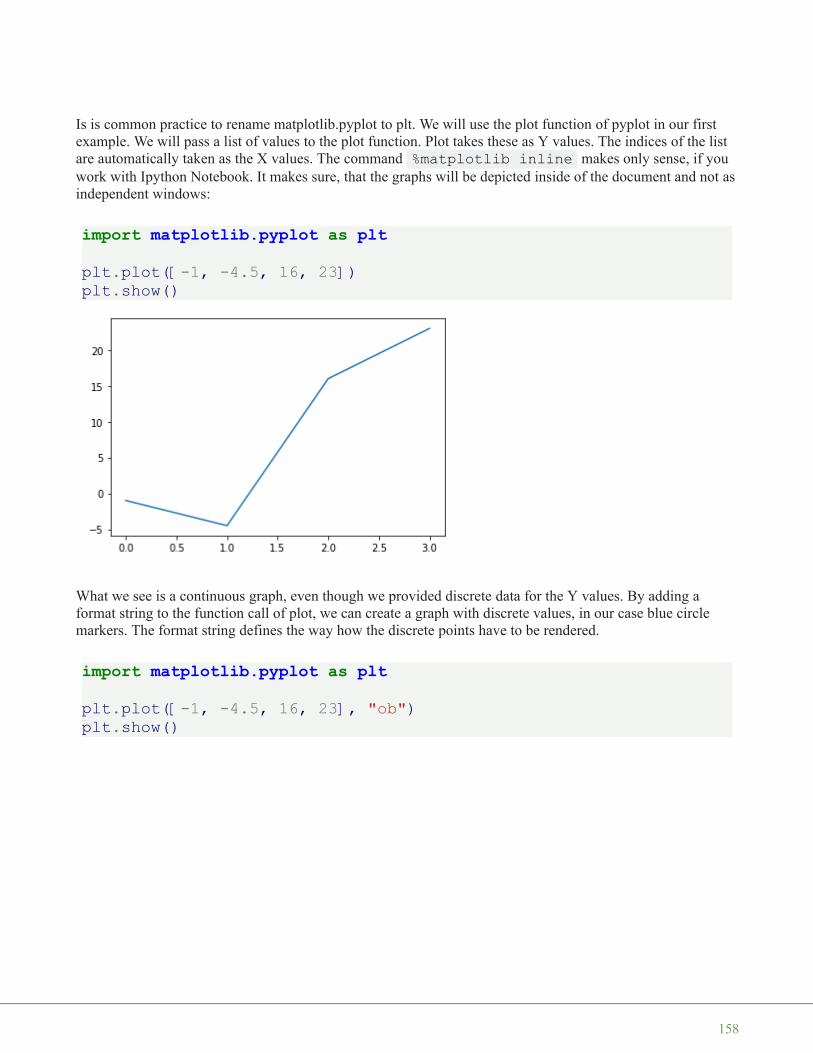
Is is common practice to rename matplotlib.pyplot to plt. We will use the plot function of pyplot in our firstexample. We will pass a list of values to the plot function. Plot takes these as Y values. The indices of the listare automatically taken as the X values. The command %matplotlib inline makes only sense, if youwork with Ipython Notebook. It makes sure, that the graphs will be depicted inside of the document and not asindependent windows:

import matplotlib.pyplot as pltplt.plot([-1, -4.5, 16, 23])plt.show()

What we see is a continuous graph, even though we provided discrete data for the Y values. By adding aformat string to the function call of plot, we can create a graph with discrete values, in our case blue circlemarkers. The format string defines the way how the discrete points have to be rendered.

import matplotlib.pyplot as pltplt.plot([-1, -4.5, 16, 23], "ob")plt.show()

158

With only a little bit of input we were capable in the previous examples to create plots. Yet, the plots missedsome information. Usually, we would like to give a name to the 'x' and 'y' values. Furthermore, the wholegraph should have a title. We demonstate this in the following example:

import matplotlib.pyplot as pltdays = range(1, 9)celsius_values = [25.6, 24.1, 26.7, 28.3, 27.5, 30.5, 32.8, 33.1]

fig, ax = plt.subplots()ax.plot(days, celsius_values)ax.set(xlabel='Day',

ylabel='Temperature in Celsius',title='Temperature Graph')

plt.show()

159

MULTIPLE PLOTS IN ONE GRAPH

We saw that the plot function is needed to plot a figure or better the figures, because there may be morethan one.

We can specify an arbitrary number of x, y, fmt groups in a one plot function. We will extend our previoustemperature example to demonstrate this. We provide two lists with temperature values, one for the minimumand one for the maximum values:

import matplotlib.pyplot as pltdays = list(range(1,9))celsius_min = [19.6, 24.1, 26.7, 28.3, 27.5, 30.5, 32.8, 33.1]celsius_max = [24.8, 28.9, 31.3, 33.0, 34.9, 35.6, 38.4, 39.2]

fig, ax = plt.subplots()

ax.set(xlabel='Day',ylabel='Temperature in Celsius',title='Temperature Graph')

ax.plot(days, celsius_min,days, celsius_min, "oy",days, celsius_max,days, celsius_max, "or")

plt.show()

160

We could have used four plot calls in the previous code instead of one, even though this is not very attractive:

import matplotlib.pyplot as pltdays = list(range(1, 9))celsius_min = [19.6, 24.1, 26.7, 28.3, 27.5, 30.5, 32.8, 33.1]celsius_max = [24.8, 28.9, 31.3, 33.0, 34.9, 35.6, 38.4, 39.2]

fig, ax = plt.subplots()

ax.set(xlabel='Day',ylabel='Temperature in Celsius',title='Temperature Graph')

ax.plot(days, celsius_min)ax.plot(days, celsius_min, "oy")ax.plot(days, celsius_max)ax.plot(days, celsius_max, "or")

plt.show()

161

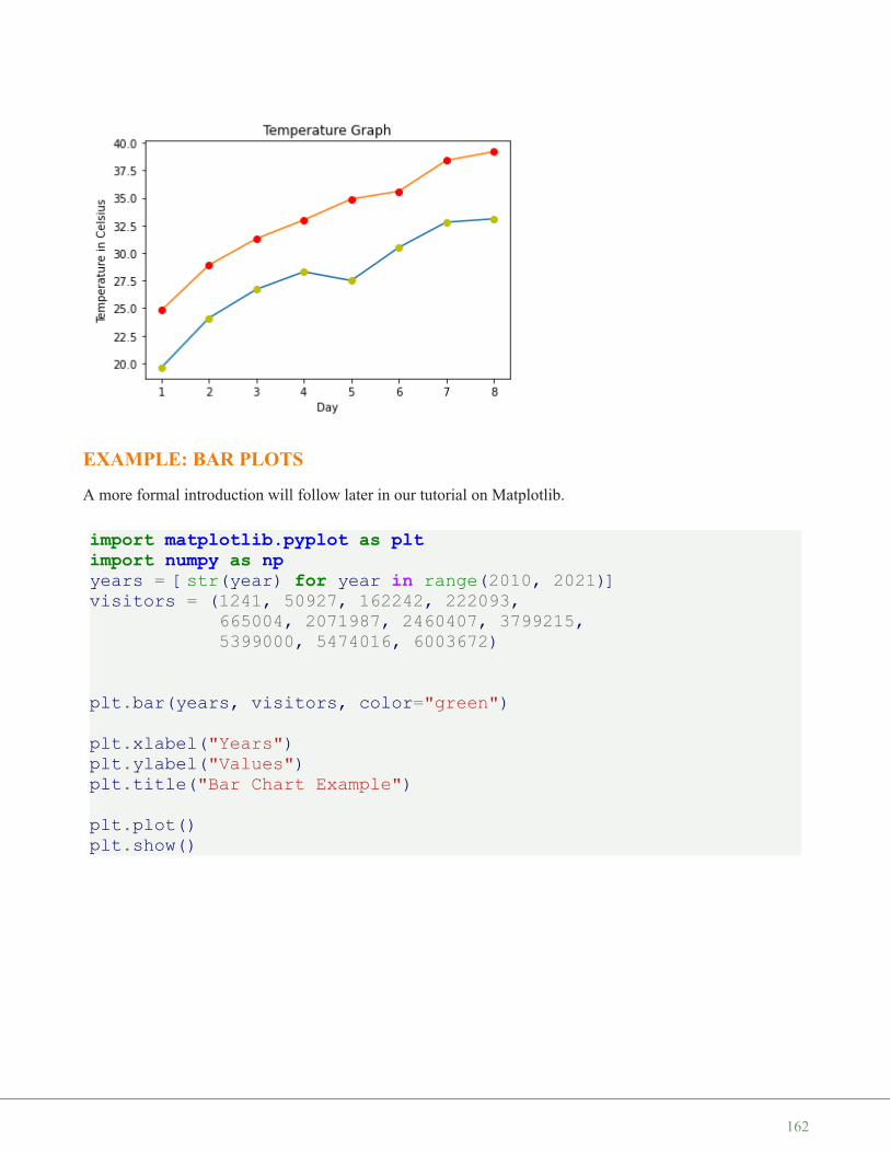
EXAMPLE: BAR PLOTS

A more formal introduction will follow later in our tutorial on Matplotlib.

import matplotlib.pyplot as pltimport numpy as npyears = [str(year) for year in range(2010, 2021)]visitors = (1241, 50927, 162242, 222093,

665004, 2071987, 2460407, 3799215,5399000, 5474016, 6003672)

plt.bar(years, visitors, color="green")

plt.xlabel("Years")plt.ylabel("Values")plt.title("Bar Chart Example")

plt.plot()plt.show()

162

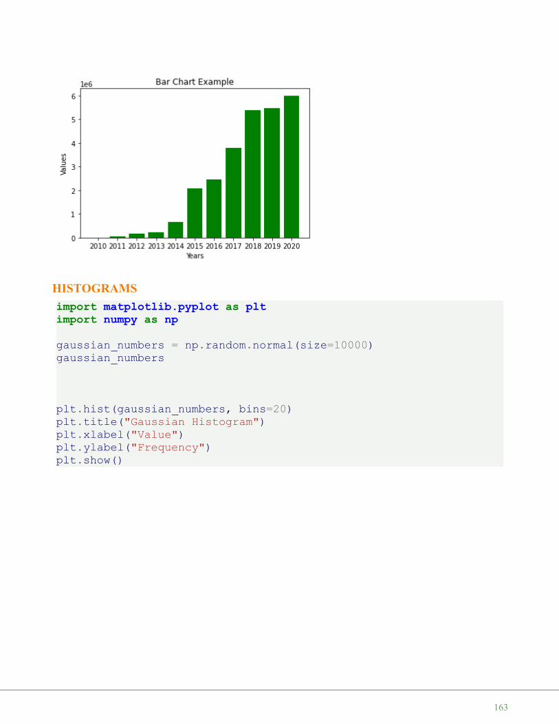
HISTOGRAMSimport matplotlib.pyplot as pltimport numpy as npgaussian_numbers = np.random.normal(size=10000)gaussian_numbers

plt.hist(gaussian_numbers, bins=20)plt.title("Gaussian Histogram")plt.xlabel("Value")plt.ylabel("Frequency")plt.show()

163

SCATTER PLOTSimport matplotlib.pyplot as pltimport numpy as npx = np.arange(0, 11)

y1 = np.random.randint(2, 7, (11,))y2 = np.random.randint(9, 14, (11,))y3 = np.random.randint(15, 25, (11,))

# Markers: https://matplotlib.org/api/markers_api.html

plt.scatter(x, y1)plt.scatter(x, y2, marker='v', color='r')plt.scatter(x, y3, marker='^', color='m')plt.title('Scatter Plot Example')plt.show()

164

STACK PLOTSimport matplotlib.pyplot as pltidxes = [ 1, 2, 3, 4, 5, 6, 7, 8, 9]y1 = [23, 42, 33, 43, 8, 44, 43, 18, 21]y2 = [9, 31, 25, 14, 17, 17, 42, 22, 28]y3 = [18, 29, 19, 22, 18, 16, 13, 32, 21]

plt.stackplot(idxes,y1, y2, y3)

plt.title('Stack Plot Example')

plt.show()

165

PIE CHARTSimport matplotlib.pyplot as plt# Pie chart, where the slices will be ordered and plotted counter-clockwise:labels = 'C', 'Python', 'Java', 'C++', 'C#'sizes = [13.38, 11.87, 11.74, 7.81, 4.41]explode = (0, 0.1, 0, 0, 0) # only "explode" the 2nd slice (i.e.'Hogs')

fig1, ax1 = plt.subplots()ax1.pie(sizes, explode=explode, labels=labels, autopct='%1.1f%%',

shadow=True, startangle=0)ax1.axis('equal') # Equal aspect ratio ensures that pie is drawnas a circle.

plt.title('TIOBE Index for May 2021')plt.show()

# Pie chart, where the slices will be ordered and plotted counter-clockwise:labels = 'C', 'Python', 'Java', 'C++', 'C#', 'others'sizes = [13.38, 11.87, 11.74, 7.81, 4.41]sizes.append(100 - sum(sizes))explode = (0, 0.1, 0, 0, 0, 0) # only "explode" the 2nd slice(i.e. 'Hogs')

fig1, ax1 = plt.subplots()ax1.pie(sizes, explode=explode, labels=labels, autopct='%1.1f%%',

shadow=True, startangle=0)

166

ax1.axis('equal') # Equal aspect ratio ensures that pie is drawnas a circle.

plt.title('TIOBE Index for May 2021')plt.show()

167

F O R M A T P L O T S

FORMAT PARAMETERimport matplotlib.pyplot as pltplt.plot([-1, -4.5, 16, 23])plt.show()

What we see is a continuous graph, even though we provided discrete data for the Y values. By adding aformat string to the function call of plot, we can create a graph with discrete values, in our case blue circlemarkers. The format string defines the way how the discrete points have to be rendered.

import matplotlib.pyplot as pltplt.plot([-1, -4.5, 16, 23], "ob")plt.show()

168

THE FORMAT PARAMETER OF PYPLOT.PLOT

We have used "ob" in our previous example as the format parameter. It consists of two characters. The firstone defines the line style or the dicrete value style, i.e. the markers, while the second one chooses a colour forthe graph. The order of the two characters could have been reversed, i.e. we could have written it as "bo" aswell. If the format parameter is not given, as in the first example, the default value is "b-", i.e. a solid blue line.

The following format string characters are accepted to control the line style or marker:

=============================================character description============================================='-' solid line style'--' dashed line style'-.' dash-dot line style':' dotted line style'.' point marker',' pixel marker'o' circle marker'v' triangle_down marker'^' triangle_up marker'<' triangle_left marker'>' triangle_right marker'1' tri_down marker'2' tri_up marker'3' tri_left marker'4' tri_right marker's' square marker'p' pentagon marker

169

'*' star marker'h' hexagon1 marker'H' hexagon2 marker'+' plus marker'x' x marker'D' diamond marker'd' thin_diamond marker'|' vline marker'_' hline marker===============================================

The following color abbreviations are supported:

==================character color=================='b' blue'g' green'r' red'c' cyan'm' magenta'y' yellow'k' black'w' white==================

As you may have guessed already, you can add X values to the plot function. We will use the multiples of 3starting at 3 below 22 as the X values of the plot in the following example:

import matplotlib.pyplot as plt# our X values:days = list(range(0, 22, 3))print("Values of days:", days)# our Y values:celsius_values = [25.6, 24.1, 26.7, 28.3, 27.5, 30.5, 32.8, 33.1]

plt.plot(days, celsius_values)plt.show()

170

... and once more with discrete values:

plt.plot(days, celsius_values, 'bo')plt.show()

Values of days: [0, 3, 6, 9, 12, 15, 18, 21]

171

M A T P L O T L I B T U T O R I A L

MATPLOTLIB OBJECT HIERARCHY AND IMPORTANT TERMS

Matplotlib is hierarchically organized. In the previous chapter,we didn't made use of this structure. All we used was a simpleplot like plt.plot([2, 5, 9]) which is implicitlybuilding the necessary structures. We didn't have to know aboutthe underlying hierarchical structure. in this chapter of ourtutorial we will explain the underlying object hierarchy. We willalso demonstrate how to use it to plot graphs and work with thecreated axes.

A matplotlib object is a tree-like structure of matplotlib objectswhich build a "hierarchy". The top of the tree-like structure ofmatplotlib objects is the figure object. A figure can be seenas the container which contains one or more plots. The plots arecalled axes in matplotlib jargon. Axes is the plural of theword "axis", which gives us a misleading idea. We can thinkabout "axes" as a synonym for the word "plot". The followingdiagram shows a figure with one axes:

As we have already mentioned a figure may also contain more than one axes:

172

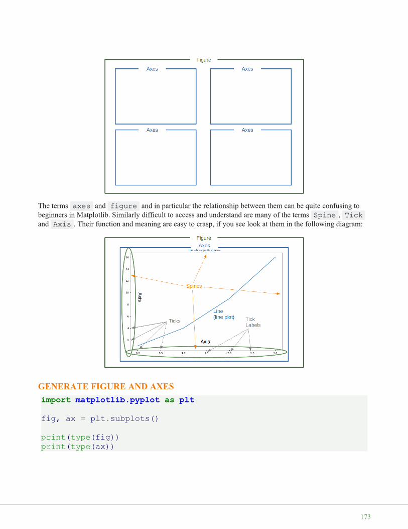
The terms axes and figure and in particular the relationship between them can be quite confusing tobeginners in Matplotlib. Similarly difficult to access and understand are many of the terms Spine , Tickand Axis . Their function and meaning are easy to crasp, if you see look at them in the following diagram:

GENERATE FIGURE AND AXESimport matplotlib.pyplot as pltfig, ax = plt.subplots()

print(type(fig))print(type(ax))

173

The function subplots can be used to create a figure and a set of subplots. In our previous example, wecalled the function without parameters which creates a figure with a single included axes. we will see laterhow to create more than one axes with subplots .

We will demonstrate in the following example, how we can go on with these objects to create a plot. We cansee that we apply plot directly on the axis object ax . This leaves no possible ambiguity as in theplt.plot approach:

import matplotlib.pyplot as plt# Data for plottingX = [2, 4, 6, 8, 10]Y = [1, 4, 9, 19, 39]

fig, ax = plt.subplots()ax.plot(X, Y)

<class 'matplotlib.figure.Figure'><class 'matplotlib.axes._subplots.AxesSubplot'>

174

LABELS ON AXES

We can improve the appearance of our graph by adding labels to the axes. We also want to give our plot aheadline or let us call it a title to stay in the terminology of Matplotlib. We can accomplish this by usingthe set method of the axis object ax :

import matplotlib.pyplot as pltdays = list(range(1,9))celsius_values = [25.6, 24.1, 26.7, 28.3, 27.5, 30.5, 32.8, 33.1]

fig, ax = plt.subplots()ax.plot(days, celsius_values)ax.set(xlabel='Day',

ylabel='Temperature in Celsius',title='Temperature Graph')

plt.show()

Output: [<matplotlib.lines.Line2D at 0x7f5dbe7b6dd8>]

175

THE PLOT FUNCTION

The plot function is needed to plot a figure or better the figures, because there may be more than one.When plot is run in ipython with its pylab mode, it displays all figures and returns to the ipython prompt.When we run it in non-interactive mode, - which is the case, when we run a Python program - it displays allfigures and blocks until the figures have been closed.

We can specify an arbitrary number of x, y, fmt groups in a plot function. We will extend our previoustemperature example to demonstrate this. We provide two lists with temperature values, one for the minimumand one for the maximum values:

import matplotlib.pyplot as pltdays = list(range(1,9))celsius_min = [19.6, 24.1, 26.7, 28.3, 27.5, 30.5, 32.8, 33.1]celsius_max = [24.8, 28.9, 31.3, 33.0, 34.9, 35.6, 38.4, 39.2]

fig, ax = plt.subplots()

ax.set(xlabel='Day',ylabel='Temperature in Celsius',title='Temperature Graph')

ax.plot(days, celsius_min,days, celsius_min, "oy",days, celsius_max,days, celsius_max, "or")

176

plt.show()

We could have used for plot calls in the previous code instead of one, even though this is not very attractive:

import matplotlib.pyplot as pltdays = list(range(1, 9))celsius_min = [19.6, 24.1, 26.7, 28.3, 27.5, 30.5, 32.8, 33.1]celsius_max = [24.8, 28.9, 31.3, 33.0, 34.9, 35.6, 38.4, 39.2]

fig, ax = plt.subplots()

ax.set(xlabel='Day',ylabel='Temperature in Celsius',title='Temperature Graph')

ax.plot(days, celsius_min)ax.plot(days, celsius_min, "oy")ax.plot(days, celsius_max)ax.plot(days, celsius_max, "or")

plt.show()

177

CHECKING AND DEFINING THE RANGE OF AXES

We can also check and define the range of the axes with the function axis. If you call it without arguments itreturns the current axis limits:

import matplotlib.pyplot as pltdays = list(range(1, 9))celsius_values = [25.6, 24.1, 26.7, 28.3, 27.5, 30.5, 32.8, 33.1]

fig, ax = plt.subplots()ax.plot(days, celsius_values)ax.set(xlabel='Day',

ylabel='Temperature in Celsius',title='Temperature Graph')

print("The current limits for the axes are:")print(ax.axis())print("We set the axes to the following values:")xmin, xmax, ymin, ymax = 0, 10, 14, 45print(xmin, xmax, ymin, ymax)ax.axis([xmin, xmax, ymin, ymax])plt.show()

178

"LINSPACE" TO DEFINE X VALUES

We will use the Numpy function linspace in the following example. linspace can be used to create evenlyspaced numbers over a specified interval.

import numpy as npimport matplotlib.pyplot as pltX = np.linspace(-2 * np.pi, 2 * np.pi, 50, endpoint=True)F1 = 3 * np.sin(X)F2 = np.sin(2*X)F3 = 0.3 * np.sin(X)

fig, ax = plt.subplots()

startx, endx = -2 * np.pi - 0.1, 2*np.pi + 0.1starty, endy = -3.1, 3.1ax.axis([startx, endx, starty, endy])

ax.plot(X, F1, X, F2, X, F3)# discrete points:ax.plot(X, F1, 'ro', X, F2, 'bx')plt.show()

The current limits for the axes are:(0.6499999999999999, 8.35, 23.650000000000002, 33.550000000000004)We set the axes to the following values:0 10 14 45

179

CHANGING THE LINE STYLE

The linestyle of a plot can be influenced with the linestyle or ls parameter of the plot function. It can be set toone of the following values:'-', '--', '-.', ':', 'None', ' ', ''

We can use linewidth to set the width of a line as the name implies.

import numpy as npimport matplotlib.pyplot as pltX = np.linspace(0, 2 * np.pi, 50, endpoint=True)F1 = 3 * np.sin(X)F2 = np.sin(2*X)F3 = 0.3 * np.sin(X)F4 = np.cos(X)

fig, ax = plt.subplots()ax.plot(X, F1, color="blue", linewidth=2.5, linestyle="-")ax.plot(X, F2, color="red", linewidth=1.5, linestyle="--")ax.plot(X, F3, color="green", linewidth=2, linestyle=":")ax.plot(X, F4, color="grey", linewidth=2, linestyle="-.")plt.show()

180

SCATTER PLOTS IN MATPLOTLIB

We will learn now how to draw single points in Matplotlib.

import matplotlib.pyplot as pltfig, ax = plt.subplots()ax.scatter(3, 7, s=42)

import matplotlib.pyplot as pltimport numpy as npX = np.random.randint(0, 100, (20,))Y = np.random.randint(0, 100, (20,))

Output: <matplotlib.collections.PathCollection at 0x7fd1ee805e20>

181

fig, ax = plt.subplots()ax.scatter(X, Y, s=42)

Output: <matplotlib.collections.PathCollection at 0x7fd1edfa16d0>

182

S H A D I N G R E G I O N S W I T H F I L L _ B E T W E E N ( )

It is possible to shade or colorize regions between two curves. We are filling the region between the X axis andthe graph of sin(2*X) in the following example:

import numpy as npimport matplotlib.pyplot as pltn = 256X = np.linspace(-np.pi,np.pi,n,endpoint=True)Y = np.sin(2*X)

fig, ax = plt.subplots()ax.plot (X, Y, color='blue', alpha=1.0)ax.fill_between(X, 0, Y, color='blue', alpha=.2)plt.show()

The general syntax of fill_between:

fill_between(x, y1, y2=0, where=None, interpolate=False, **kwargs)

The parameters of fill_between:

183

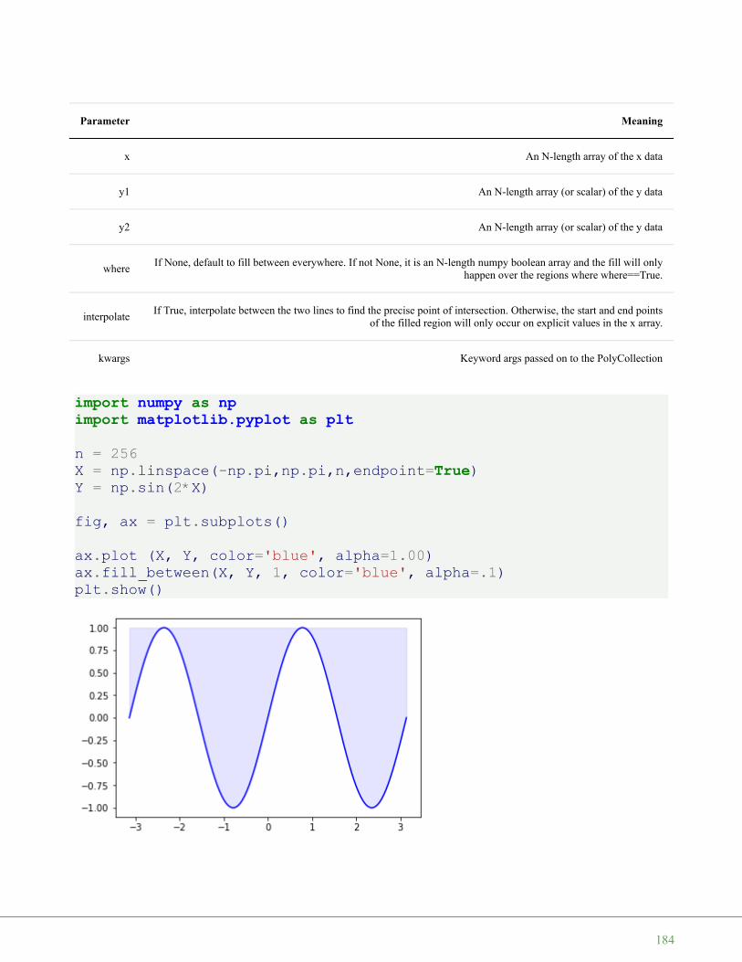
Parameter Meaning

x An N-length array of the x data

y1 An N-length array (or scalar) of the y data

y2 An N-length array (or scalar) of the y data

whereIf None, default to fill between everywhere. If not None, it is an N-length numpy boolean array and the fill will only

happen over the regions where where==True.

interpolateIf True, interpolate between the two lines to find the precise point of intersection. Otherwise, the start and end points

of the filled region will only occur on explicit values in the x array.

kwargs Keyword args passed on to the PolyCollection

import numpy as npimport matplotlib.pyplot as pltn = 256X = np.linspace(-np.pi,np.pi,n,endpoint=True)Y = np.sin(2*X)

fig, ax = plt.subplots()

ax.plot (X, Y, color='blue', alpha=1.00)ax.fill_between(X, Y, 1, color='blue', alpha=.1)plt.show()

184

185

M A T P L O T L I B T U T O R I A L : S P I N E S A N DT I C K S

MOVING THE BORDER LINES AND POLISHING UP THE AXES NOTATIONS

The word spine is most commonly known as the backbone or spinalcord of the human skeleton. Another meaning stands for a book'sjacket. Our picture on the right side shows the spines of a cactus,artistically changed into something which looks like a ribcage. You willhardly find the usage of the word spine of matplotlib in adictionary. Spines in matplotlib are the lines connecting the axis tickmarks and noting the boundaries of the data area.

We will demonstrate in the following that the spines can be placed atarbitrary positions.

We will move around the spines in the course of this chapter so that theform a 'classical' coordinate syste. One where we have a x axis and a yaxis and both go through the origin i.e. the point (0, 0)

We will show the naming of the spines in the following diagram:

186

We will move the spines to build a 'classical' coordinate system. To this purpose we turn the top and rightspine invisible and move the bottom and left one around:

# the next "inline" statement is only needed,# if you are working with "ipython notebook"%matplotlib inline

import numpy as npimport matplotlib.pyplot as pltX = np.linspace(-2 * np.pi, 2 * np.pi, 70, endpoint=True)F1 = np.sin(2* X)F2 = (2*X**5 + 4*X**4 - 4.8*X**3 + 1.2*X**2 + X + 1)*np.exp(-X**2)

fig, ax = plt.subplots()

# making the top and right spine invisible:ax.spines['top'].set_color('none')ax.spines['right'].set_color('none')

187

# moving bottom spine up to y=0 position:ax.xaxis.set_ticks_position('bottom')ax.spines['bottom'].set_position(('data',0))

# moving left spine to the right to position x == 0:ax.yaxis.set_ticks_position('left')ax.spines['left'].set_position(('data',0))

ax.plot(X, F1, X, F2)

plt.show()

CUSTOMIZING TICKS

Matplotlib has so far - in all our previous examples - automatically taken over the task of spacing points on theaxis. We can see for example that the X axis in our previous example was numbered -6. -4, -2, 0,2, 4, 6 , whereas the Y axis was numbered -1.0, 0, 1.0, 2.0, 3.0

xticks is a method, which can be used to get or to set the current tick locations and the labels. The same is truefor yticks:

import matplotlib.pyplot as pltfig, ax = plt.subplots()

xticks = ax.get_xticks()xticklabels = ax.get_xticklabels()print(xticks, xticklabels)for i in range(6):

print(xticklabels[i])

188

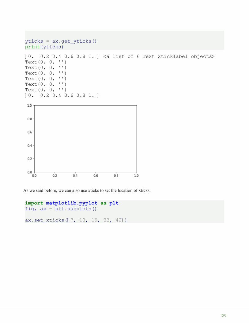
yticks = ax.get_yticks()print(yticks)

As we said before, we can also use xticks to set the location of xticks:

import matplotlib.pyplot as pltfig, ax = plt.subplots()

ax.set_xticks([7, 13, 19, 33, 42])

[0. 0.2 0.4 0.6 0.8 1. ] <a list of 6 Text xticklabel objects>Text(0, 0, '')Text(0, 0, '')Text(0, 0, '')Text(0, 0, '')Text(0, 0, '')Text(0, 0, '')[0. 0.2 0.4 0.6 0.8 1. ]

189

Now, we will set both the locations and the labels of the xticks:

import matplotlib.pyplot as pltfig, ax = plt.subplots()

ax.set_xticks([7, 13, 19, 33, 42])ax.set_xticklabels(['Berlin', 'London', 'Hamburg', 'Toronto'])

Output: [<matplotlib.axis.XTick at 0x7f8a1e5bd080>,<matplotlib.axis.XTick at 0x7f8a1e5bdd68>,<matplotlib.axis.XTick at 0x7f8a1e2237b8>,<matplotlib.axis.XTick at 0x7f8a1e592a20>,<matplotlib.axis.XTick at 0x7f8a1e5921d0>]

190

Let's get back to our previous example with the trigonometric functions. Most people might consider factors ofPi to be more appropriate for the X axis than the integer labels:

import numpy as npimport matplotlib.pyplot as pltX = np.linspace(-2 * np.pi, 2 * np.pi, 70, endpoint=True)X = np.linspace(-2 * np.pi, 2 * np.pi, 70, endpoint=True)F1 = np.sin(X**2)F2 = X * np.sin(X)

fig, ax = plt.subplots()

# making the top and right spine invisible:ax.spines['top'].set_color('none')ax.spines['right'].set_color('none')# moving bottom spine up to y=0 position:ax.xaxis.set_ticks_position('bottom')ax.spines['bottom'].set_position(('data',0))# moving left spine to the right to position x == 0:ax.yaxis.set_ticks_position('left')ax.spines['left'].set_position(('data',0))

ax.set_xticks( [-6.28, -3.14, 3.14, 6.28])ax.set_yticks([-3, -1, 0, +1, 3])

Output: [Text(0, 0, 'Berlin'),Text(0, 0, 'London'),Text(0, 0, 'Hamburg'),Text(0, 0, 'Toronto')]

191

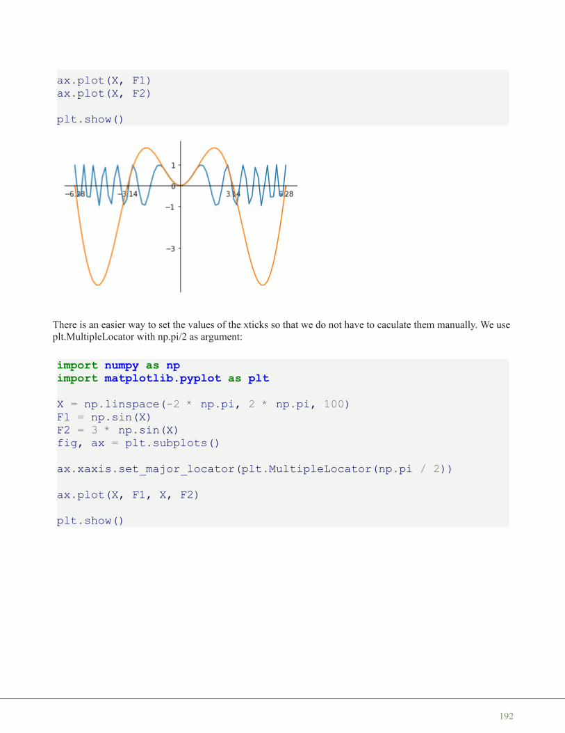
ax.plot(X, F1)ax.plot(X, F2)

plt.show()

There is an easier way to set the values of the xticks so that we do not have to caculate them manually. We useplt.MultipleLocator with np.pi/2 as argument:

import numpy as npimport matplotlib.pyplot as pltX = np.linspace(-2 * np.pi, 2 * np.pi, 100)F1 = np.sin(X)F2 = 3 * np.sin(X)fig, ax = plt.subplots()

ax.xaxis.set_major_locator(plt.MultipleLocator(np.pi / 2))

ax.plot(X, F1, X, F2)

plt.show()

192

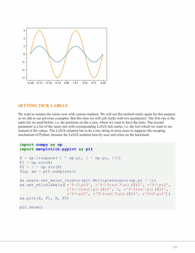
SETTING TICK LABELS

We want to rename the xticks now with custom markers. We will use the method xticks again for this purposeas we did in our previous examples. But this time we will call xticks with two parameters: The first one is thesame list we used before, i.e. the positions on the x axis, where we want to have the ticks. The secondparameter is a list of the same size with corresponding LaTeX tick marks, i.e. the text which we want to seeinstead of the values. The LaTeX notation has to be a raw string in most cases to suppress the escapingmechanism of Python, because the LaTeX notation heavily uses and relies on the backslash.

import numpy as npimport matplotlib.pyplot as pltX = np.linspace(-2 * np.pi, 2 * np.pi, 100)F1 = np.sin(X)F2 = 3 * np.sin(X)fig, ax = plt.subplots()

ax.xaxis.set_major_locator(plt.MultipleLocator(np.pi / 2))ax.set_xticklabels([r'$-2\pi$', r'$-\frac{3\pi}{2}$', r'$-\pi$',

r'$-\frac{\pi}{2}$', 0, r'$\frac{\pi}{2}$',r'$+\pi$', r'$\frac{3\pi}{2}$', r'$+2\pi$'])

ax.plot(X, F1, X, F2)

plt.show()

193

ADJUSTING THE TICKLABELS

We want to increase the legibility of the ticklabels. We will increase the font size, and we will render them ona semi transparant background.

print(ax.get_xticklabels())

for xtick in ax.get_xticklabels():print(xtick)

labels = [xtick.get_text() for xtick in ax.get_xticklabels()]print(labels)

Let's increase the fontsize and make the font semi transparant:

import numpy as npimport matplotlib.pyplot as pltX = np.linspace(-2 * np.pi, 2 * np.pi, 170, endpoint=True)

<a list of 4 Text xticklabel objects>

Text(-6.28, 0, '$-2\\pi$')Text(-3.14, 0, '$-\\pi$')Text(3.14, 0, '$+\\pi$')Text(6.28, 0, '$+2\\pi$')

['$-2\\pi$', '$-\\pi$', '$+\\pi$', '$+2\\pi$']

194

F1 = np.sin(X**3 / 2)

fig, ax = plt.subplots()

ax.xaxis.set_major_locator(plt.MultipleLocator(np.pi / 2))ax.set_xticklabels([r'$-2\pi$', r'$-\frac{3\pi}{2}$', r'$-\pi$',

r'$-\frac{\pi}{2}$', 0, r'$\frac{\pi}{2}$',r'$+\pi$', r'$\frac{3\pi}{2}$', r'$+2\pi$'])

for xtick in ax.get_xticklabels():xtick.set_fontsize(18)xtick.set_bbox(dict(facecolor='white', edgecolor='None', alph

a=0.7 ))

for ytick in ax.get_yticklabels():ytick.set_fontsize(14)ytick.set_bbox(dict(facecolor='white', edgecolor='None', alph

a=0.7 ))

ax.plot(X, F1, label="$sin(x)$")

ax.legend(loc='lower left')

plt.show()

195

196

M A T P L O T L I B T U T O R I A L , A D D I N G L E G E N D SA N D A N N O T A T I O N S

ADDING A LEGEND

This chapter of our tutorial is about legends. Legends are theclassical stories from ancient Greece or other places which areusually devoured by adolescents. They have to read it and this iswhere the original meaning comes from. The word legendstems from Latin and it means in Latin "to be read". So we cansay legends are the things in a graph or plot which have to beread to understand the plot. It gives us valuable informationabout the visualized data.

Before legends have been used in mathematical graphs, theyhave been used in maps. Legends - as they are found in maps -describe the pictorial language or symbology of the map.Legends are used in line graphs to explain the function or thevalues underlying the different lines of the graph.

We will demonstrate in the following simple example how wecan place a legend on a graph. A legend contains one or more entries. Every entry consists of a key and alabel.

The pyplot function

legend(*args, **kwargs)

places a legend on the axes.

All we have to do to create a legend for lines, which already exist on the axes, is to simply call the function"legend" with an iterable of strings, one for each legend item.

We have mainly used trigonometric functions in our previous chapter. For a change we want to use nowpolynomials. We will use the Polynomial class which we have defined in our chapter Polynomials.

# the module polynomials can be downloaded from# https://www.python-course.eu/examples/polynomials.pyfrom polynomials import Polynomialimport numpy as npimport matplotlib.pyplot as pltp = Polynomial(-0.8, 2.3, 0.5, 1, 0.2)p_der = p.derivative()

197

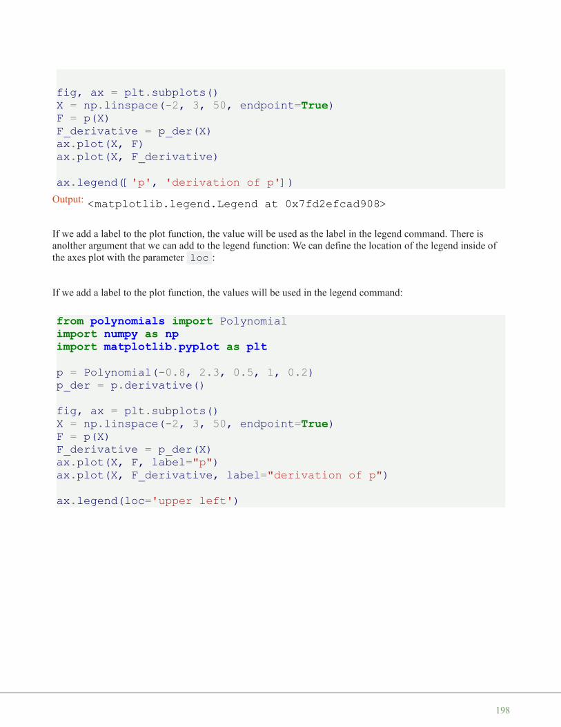
fig, ax = plt.subplots()X = np.linspace(-2, 3, 50, endpoint=True)F = p(X)F_derivative = p_der(X)ax.plot(X, F)ax.plot(X, F_derivative)

ax.legend(['p', 'derivation of p'])

If we add a label to the plot function, the value will be used as the label in the legend command. There isanolther argument that we can add to the legend function: We can define the location of the legend inside ofthe axes plot with the parameter loc :

If we add a label to the plot function, the values will be used in the legend command:

from polynomials import Polynomialimport numpy as npimport matplotlib.pyplot as pltp = Polynomial(-0.8, 2.3, 0.5, 1, 0.2)p_der = p.derivative()

fig, ax = plt.subplots()X = np.linspace(-2, 3, 50, endpoint=True)F = p(X)F_derivative = p_der(X)ax.plot(X, F, label="p")ax.plot(X, F_derivative, label="derivation of p")

ax.legend(loc='upper left')

Output: <matplotlib.legend.Legend at 0x7fd2efcad908>

198

It might be even more interesting to see the actual function in mathematical notation in our legend. Ourpolynomial class is capable of printing the function in LaTeX notation.

print(p)print(p_der)

We can also use LaTeX in our labels, if we include it in '$' signs.

from polynomials import Polynomialimport numpy as npimport matplotlib.pyplot as pltp = Polynomial(2, 3, -4, 6)p_der = p.derivative()

fig, ax = plt.subplots()X = np.linspace(-2, 3, 50, endpoint=True)F = p(X)F_derivative = p_der(X)ax.plot(X, F, label="$" + str(p) + "$")ax.plot(X, F_derivative, label="$" + str(p_der) + "$")

ax.legend(loc='upper left')

Output: <matplotlib.legend.Legend at 0x7fd2efc15cf8>

-0.8x^4 + 2.3x^3 + 0.5x^2 + 1x^1 + 0.2-3.2x^3 + 6.8999999999999995x^2 + 1.0x^1 + 1

199

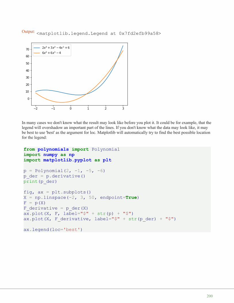
In many cases we don't know what the result may look like before you plot it. It could be for example, that thelegend will overshadow an important part of the lines. If you don't know what the data may look like, it maybe best to use 'best' as the argument for loc. Matplotlib will automatically try to find the best possible locationfor the legend:

from polynomials import Polynomialimport numpy as npimport matplotlib.pyplot as pltp = Polynomial(2, -1, -5, -6)p_der = p.derivative()print(p_der)

fig, ax = plt.subplots()X = np.linspace(-2, 3, 50, endpoint=True)F = p(X)F_derivative = p_der(X)ax.plot(X, F, label="$" + str(p) + "$")ax.plot(X, F_derivative, label="$" + str(p_der) + "$")

ax.legend(loc='best')

Output: <matplotlib.legend.Legend at 0x7fd2efb99a58>

200

We will go back to trigonometric functions in the following examples. These examples show that

loc='best'

can work pretty well:

import numpy as npimport matplotlib.pyplot as pltX = np.linspace(-2 * np.pi, 2 * np.pi, 70, endpoint=True)F1 = np.sin(0.5*X)F2 = -3 * np.cos(0.8*X)

plt.xticks( [-6.28, -3.14, 3.14, 6.28],[r'$-2\pi$', r'$-\pi$', r'$+\pi$', r'$+2\pi$'])

plt.yticks([-3, -1, 0, +1, 3])plt.plot(X, F1, label="$sin(0.5x)$")plt.plot(X, F2, label="$-3 cos(0.8x)$")plt.legend(loc='best')

plt.show()

6x^2 - 2x^1 - 5Output: <matplotlib.legend.Legend at 0x7fd2ef370f60>

201

import numpy as npimport matplotlib.pyplot as pltX = np.linspace(-2 * np.pi, 2 * np.pi, 70, endpoint=True)F1 = np.sin(0.5*X)F2 = 3 * np.cos(0.8*X)

plt.xticks( [-6.28, -3.14, 3.14, 6.28],[r'$-2\pi$', r'$-\pi$', r'$+\pi$', r'$+2\pi$'])

plt.yticks([-3, -1, 0, +1, 3])plt.plot(X, F1, label="$sin(0.5x)$")plt.plot(X, F2, label="$3 cos(0.8x)$")plt.legend(loc='best')

plt.show()

202

ANNOTATIONS

The visualizations of function plots often makes annotations necessary. This means we draw the readersattentions to important points and areas of the plot. To this purpose we use texts, labels and arrows. We havealready used axis labels and titles for this purpose, but these are 'annotations' for the whole plot. We can easilyannotate points inside the axis or on the graph with the annotate method of an axes object. In anannotation, there are two points to consider: the location being annotated represented by the argument xy andthe location of the text xytext. Both of these arguments are (x,y) tuples.

We demonstrate how easy it is in matplotlib to to annotate plots in matplotlib with the annotate method. Wewill annotate the local maximum and the local minimum of a function. In its simplest form annotatemethod needs two arguments annotate(s, xy) , where s is the text string for the annotation and xxis the position of the point to be annotated:

from polynomials import Polynomialimport numpy as npimport matplotlib.pyplot as pltp = Polynomial(1, 0, -12, 0)p_der = p.derivative()

fig, ax = plt.subplots()X = np.arange(-5, 5, 0.1)F = p(X)

F_derivative = p_der(X)ax.grid()

maximum = (-2, p(-2))minimum = (2, p(2))ax.annotate("local maximum", maximum)ax.annotate("local minimum", minimum)

ax.plot(X, F, label="p")ax.plot(X, F_derivative, label="derivation of p")

ax.legend(loc='best')plt.show()

203

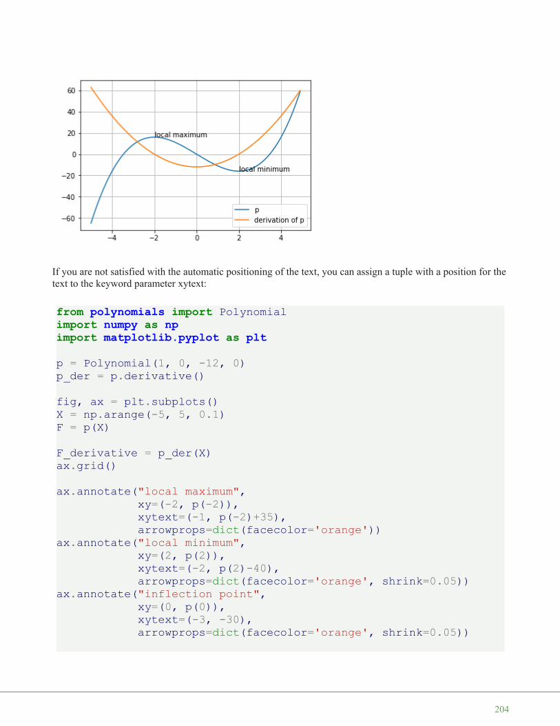
If you are not satisfied with the automatic positioning of the text, you can assign a tuple with a position for thetext to the keyword parameter xytext:

from polynomials import Polynomialimport numpy as npimport matplotlib.pyplot as pltp = Polynomial(1, 0, -12, 0)p_der = p.derivative()

fig, ax = plt.subplots()X = np.arange(-5, 5, 0.1)F = p(X)

F_derivative = p_der(X)ax.grid()

ax.annotate("local maximum",xy=(-2, p(-2)),xytext=(-1, p(-2)+35),arrowprops=dict(facecolor='orange'))

ax.annotate("local minimum",xy=(2, p(2)),xytext=(-2, p(2)-40),arrowprops=dict(facecolor='orange', shrink=0.05))

ax.annotate("inflection point",xy=(0, p(0)),xytext=(-3, -30),arrowprops=dict(facecolor='orange', shrink=0.05))

204

ax.plot(X, F, label="p")ax.plot(X, F_derivative, label="derivation of p")

ax.legend(loc='best')plt.show()

We have to provide some informations to the parameters of annotate, we have used in our previous example.

Parameter Meaning

xy coordinates of the arrow tip

xytext coordinates of the text location

The xy and the xytext locations of our example are in data coordinates. There are other coordinate systemsavailable we can choose. The coordinate system of xy and xytext can be specified string values assigned toxycoords and textcoords. The default value is 'data':

String Value Coordinate System

figure points points from the lower left corner of the figure

figure pixels pixels from the lower left corner of the figure

figure fraction 0,0 is lower left of figure and 1,1 is upper right

axes points points from lower left corner of axes

205

String Value Coordinate System

axes pixels pixels from lower left corner of axes

axes fraction 0,0 is lower left of axes and 1,1 is upper right

data use the axes data coordinate system

Additionally, we can also specify the properties of the arrow. To do so, we have to provide a dictionary ofarrow properties to the parameter arrowprops:

arrowprops key description

width the width of the arrow in points

headlength The length of the arrow head in points

headwidth the width of the base of the arrow head in points

shrink move the tip and base some percent away from the annotated point and text

**kwargs any key for matplotlib.patches.Polygon, e.g., facecolor

Of course, the sinus function has "boring" and interesting values. Let's assume that you are especiallyinterested in the value of 3 ∗ sin(3 ∗ pi /4).

import numpy as npprint(3 * np.sin(3 * np.pi/4))

The numerical result doesn't look special, but if we do a symbolic calculation for the above expression we get3

√2. Now we want to label this point on the graph. We can do this with the annotate function. We want to

annotate our graph with this point.

import numpy as npimport matplotlib.pyplot as pltX = np.linspace(-2 * np.pi, 2 * np.pi, 100)F1 = np.sin(X)

2.121320343559643

206

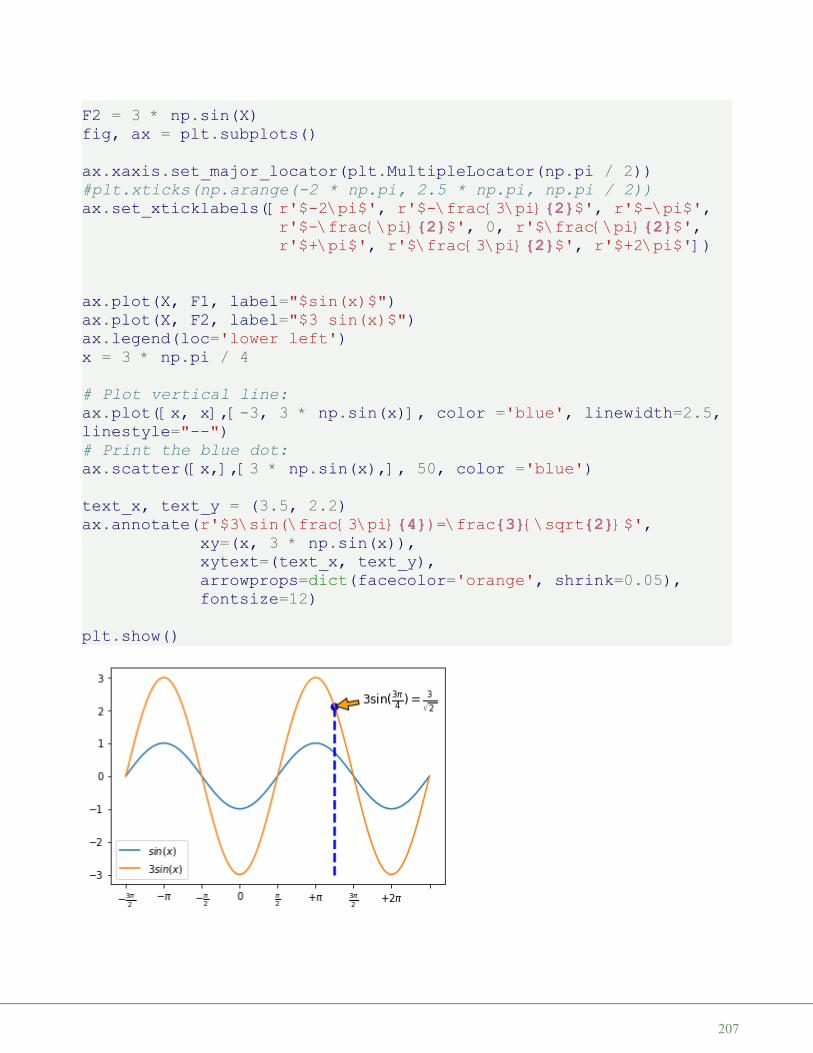
F2 = 3 * np.sin(X)fig, ax = plt.subplots()

ax.xaxis.set_major_locator(plt.MultipleLocator(np.pi / 2))#plt.xticks(np.arange(-2 * np.pi, 2.5 * np.pi, np.pi / 2))ax.set_xticklabels([r'$-2\pi$', r'$-\frac{3\pi}{2}$', r'$-\pi$',

r'$-\frac{\pi}{2}$', 0, r'$\frac{\pi}{2}$',r'$+\pi$', r'$\frac{3\pi}{2}$', r'$+2\pi$'])

ax.plot(X, F1, label="$sin(x)$")ax.plot(X, F2, label="$3 sin(x)$")ax.legend(loc='lower left')x = 3 * np.pi / 4

# Plot vertical line:ax.plot([x, x],[-3, 3 * np.sin(x)], color ='blue', linewidth=2.5,linestyle="--")# Print the blue dot:ax.scatter([x,],[3 * np.sin(x),], 50, color ='blue')

text_x, text_y = (3.5, 2.2)ax.annotate(r'$3\sin(\frac{3\pi}{4})=\frac{3}{\sqrt{2}}$',

xy=(x, 3 * np.sin(x)),xytext=(text_x, text_y),arrowprops=dict(facecolor='orange', shrink=0.05),fontsize=12)

plt.show()

207

SOME MORE CURVE SKETCHING

There is anothe example, in which we play around with the arrows and annoate the extrema.

import numpy as npimport matplotlib.pyplot as pltX = np.linspace(-4.1, 3.1, 150, endpoint=True)F = X**5 + 3*X**4 - 11*X**3 - 27*X**2 + 10*X + 24

fig, ax = plt.subplots()ax.plot(X, F)

minimum1 = -1.5264814, -7.051996717492152minimum2 = 2.3123415793720303, -81.36889464201387ax.annotate("minima",

xy=minimum1,xytext=(-1.5, -50),arrowprops=dict(arrowstyle="->",

connectionstyle="angle3,angleA=0,angleB=-90"))ax.annotate(" ",

xy=minimum2,xytext=(-0.7, -50),arrowprops=dict(arrowstyle="->",

connectionstyle="angle3,angleA=0,angleB=-90"))

maximum1 = -3.35475845886632, 56.963107876630595maximum2 = .16889828232847673, 24.868343482875485ax.annotate("maxima", xy=maximum1,

xytext=(-1.5, 30),arrowprops=dict(arrowstyle="->",

connectionstyle="angle3,angleA=0,angleB=-90"))ax.annotate(" ", xy=maximum2,

xytext=(-0.6, 30),arrowprops=dict(arrowstyle="->",

connectionstyle="angle3,angleA=0,angleB=-90"))

zeroes = -4, -2, -1, 1, 3for zero in zeroes:

zero = zero, 0

208

ax.annotate("Zeroes",xy=zero,color="orange",bbox=dict(boxstyle="round", fc="none", ec="gree

n"),xytext=(1, 40),arrowprops=dict(arrowstyle="->", color="orange",

connectionstyle="angle3,angleA=0,angleB=-90"))

plt.show()

The following program visualizes the various arrowstyles:

import matplotlib.pyplot as plt

def demo_con_style(ax, connectionstyle):x1, y1 = 0.3, 0.2x2, y2 = 0.8, 0.6

ax.plot([x1, x2], [y1, y2], ".")ax.annotate("",

xy=(x1, y1), xycoords='data',xytext=(x2, y2), textcoords='data',arrowprops=dict(arrowstyle="->", color="0.5",

shrinkA=5, shrinkB=5,patchA=None, patchB=None,connectionstyle=connectionstyle))

209

ax.text(.05, .95, connectionstyle.replace(",", ",\n"),transform=ax.transAxes, ha="left", va="top")

fig, axs = plt.subplots(3, 5, figsize=(8, 4.8))demo_con_style(axs[0, 0], "angle3,angleA=90,angleB=0")demo_con_style(axs[1, 0], "angle3,angleA=0,angleB=90")demo_con_style(axs[0, 1], "arc3,rad=0.")demo_con_style(axs[1, 1], "arc3,rad=0.3")demo_con_style(axs[2, 1], "arc3,rad=-0.3")demo_con_style(axs[0, 2], "angle,angleA=-90,angleB=180,rad=0")demo_con_style(axs[1, 2], "angle,angleA=-90,angleB=180,rad=5")demo_con_style(axs[2, 2], "angle,angleA=-90,angleB=10,rad=5")demo_con_style(axs[0, 3], "arc,angleA=-90,angleB=0,armA=30,armB=30,rad=0")demo_con_style(axs[1, 3], "arc,angleA=-90,angleB=0,armA=30,armB=30,rad=5")demo_con_style(axs[2, 3], "arc,angleA=-90,angleB=0,armA=0,armB=40,rad=0")demo_con_style(axs[0, 4], "bar,fraction=0.3")demo_con_style(axs[1, 4], "bar,fraction=-0.3")demo_con_style(axs[2, 4], "bar,angle=180,fraction=-0.2")

for ax in axs.flat:ax.set(xlim=(0, 1), ylim=(0, 1), xticks=[], yticks=[], aspec

t=1)fig.tight_layout(pad=0.2)

plt.show()

210

211

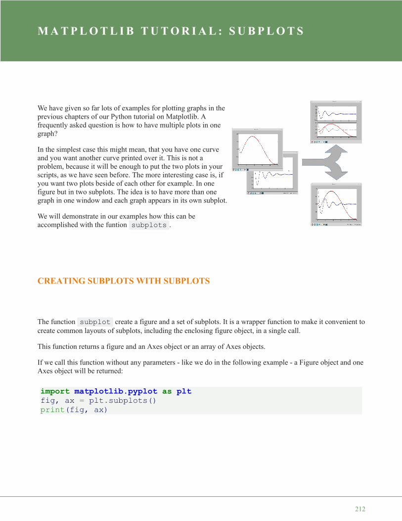
M A T P L O T L I B T U T O R I A L : S U B P L O T S

We have given so far lots of examples for plotting graphs in theprevious chapters of our Python tutorial on Matplotlib. Afrequently asked question is how to have multiple plots in onegraph?

In the simplest case this might mean, that you have one curveand you want another curve printed over it. This is not aproblem, because it will be enough to put the two plots in yourscripts, as we have seen before. The more interesting case is, ifyou want two plots beside of each other for example. In onefigure but in two subplots. The idea is to have more than onegraph in one window and each graph appears in its own subplot.

We will demonstrate in our examples how this can beaccomplished with the funtion subplots .

CREATING SUBPLOTS WITH SUBPLOTS

The function subplot create a figure and a set of subplots. It is a wrapper function to make it convenient tocreate common layouts of subplots, including the enclosing figure object, in a single call.

This function returns a figure and an Axes object or an array of Axes objects.

If we call this function without any parameters - like we do in the following example - a Figure object and oneAxes object will be returned:

import matplotlib.pyplot as pltfig, ax = plt.subplots()print(fig, ax)

212

The parameter of subplots function are:

subplots(nrows=1, ncols=1, sharex=False, sharey=False, squeeze=True,subplot_kw=None, gridspec_kw=None, **fig_kw)

Parameter Meaning

nrows, ncolsint, optional, default: 1

Number of rows/columns of the subplot grid.

sharex

bool or {'none', 'all', 'row', 'col'}, default: FalseControls sharing of properties among x ( sharex ) axis: If sharex is set to True or all , the x-axis will

be shared among all subplots. If sharex is set to False or none , each x-axis of a subplot will beindependent. If it is set to row , each subplot row will share an x-axis. If it is set to col , each subplot column

will share an x-axis.

sharey

analogue to sharexWhen subplots have a shared x-axis along a column, only the x tick labels of the bottom subplot are created.

Similarly, when subplots have a shared y-axis along a row, only the y tick labels of the first column subplot arecreated.

squeezebool, optional, default: True

If squeeze is set to True , extra dimensions are squeezed out from the returned Axes object

numinteger or string, optional, default: None

A .pyplot.figure keyword that sets the figure number or label.

subplot_kwdict, optional

Dict with keywords passed to the ~matplotlib.figure.Figure.add_subplot call used to create each

Figure(432x288) AxesSubplot(0.125,0.125;0.775x0.755)

213

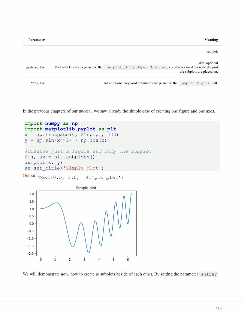
Parameter Meaning

subplot.

gridspec_kwdict, optional

Dict with keywords passed to the ~matplotlib.gridspec.GridSpec constructor used to create the gridthe subplots are placed on.

**fig_kw All additional keyword arguments are passed to the .pyplot.figure call.

In the previous chapters of our tutorial, we saw already the simple case of creating one figure and one axes.

import numpy as npimport matplotlib.pyplot as pltx = np.linspace(0, 2*np.pi, 400)y = np.sin(x**2) + np.cos(x)

#Creates just a figure and only one subplotfig, ax = plt.subplots()ax.plot(x, y)ax.set_title('Simple plot')

We will demonstrate now, how to create to subplots beside of each other. By setting the parameter sharey

Output: Text(0.5, 1.0, 'Simple plot')

214

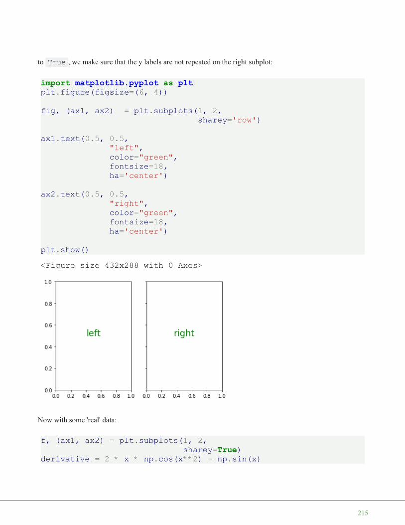
to True , we make sure that the y labels are not repeated on the right subplot:

import matplotlib.pyplot as pltplt.figure(figsize=(6, 4))

fig, (ax1, ax2) = plt.subplots(1, 2,sharey='row')

ax1.text(0.5, 0.5,"left",color="green",fontsize=18,ha='center')

ax2.text(0.5, 0.5,"right",color="green",fontsize=18,ha='center')

plt.show()

Now with some 'real' data:

f, (ax1, ax2) = plt.subplots(1, 2,sharey=True)

derivative = 2 * x * np.cos(x**2) - np.sin(x)

<Figure size 432x288 with 0 Axes>

215

ax1.plot(x, y)ax1.set_title('Sharing Y axis')ax2.plot(x, derivative)

We demonstrate in the following example how to create a subplot for polar plotting. We achieve this bycreating a key polar in the the subplot_kw dictionary and set it to True :

fig, ax = plt.subplots(1, subplot_kw=dict(polar=True))ax.plot(x, np.sin(x) * np.cos(x), "--g")

Output: [<matplotlib.lines.Line2D at 0x7fc9509f7a90>]

Output: [<matplotlib.lines.Line2D at 0x7fc9519bb650>]

216

The first two parameters of subplots define the numbers of rows and columns respectively. Wedemonstrate this in the following example. To demonstrate the structure we use the text method of the axisobjects. We use it to put the

import matplotlib.pyplot as pltrows, cols = 2, 3fig, ax = plt.subplots(rows, cols,

sharex='col',sharey='row')

for row in range(rows):for col in range(cols):

ax[row, col].text(0.5, 0.5,str((row, col)),color="green",fontsize=18,ha='center')

plt.show()

import matplotlib.pyplot as plt#plt.figure(figsize=(6, 4))

fig, ax = plt.subplots(2,sharex='col', sharey='row')

ax[0].text(0.5, 0.5,"top",color="green",

217

fontsize=18,ha='center')

ax[1].text(0.5, 0.5,"bottom",color="green",fontsize=18,ha='center')

plt.show()

We will create now a similar structure with two subplots on top of each other containing polar plots:

fig, axes = plt.subplots(2, 2, subplot_kw=dict(polar=True))axes[0, 0].plot(x, y)axes[0, 1].plot(x, np.sin(x**2) + np.cos(x**3))axes[1, 0].plot(x, np.cos(x) * np.sin(x**2))axes[1, 1].plot(x, derivative, "g--")

218

Now with titles for subplots:

import numpy as npimport matplotlib.pyplot as pltplt.figure(figsize=(6, 4))

def f(x):return np.sin(x) - x * np.cos(x)

def fp(x):""" The derivative of f """return x * np.sin(x)

X = np.arange(-5, 5.0, 0.05)

fig, ax = plt.subplots(2,sharex='col', sharey='row')

ax[0].plot(X, f(X), 'bo', X, f(X), 'k')ax[0].set(title='The function f')

ax[1].plot(X, fp(X), 'go', X, fp(X), 'k')ax[1].set(xlabel='X Values', ylabel='Y Values',

title='Derivative Function of f')

plt.show()

Output: [<matplotlib.lines.Line2D at 0x7fc9506cdad0>]

219

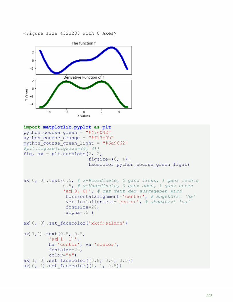
import matplotlib.pyplot as pltpython_course_green = "#476042"python_course_orange = "#f17c0b"python_course_green_light = "#6a9662"#plt.figure(figsize=(6, 4))fig, ax = plt.subplots(2, 2,

figsize=(6, 4),facecolor=python_course_green_light)

ax[0, 0].text(0.5, # x-Koordinate, 0 ganz links, 1 ganz rechts0.5, # y-Koordinate, 0 ganz oben, 1 ganz unten'ax[0, 0]', # der Text der ausgegeben wirdhorizontalalignment='center', # abgekürzt 'ha'verticalalignment='center', # abgekürzt 'va'fontsize=20,alpha=.5 )

ax[0, 0].set_facecolor('xkcd:salmon')

ax[1,1].text(0.5, 0.5,'ax[1, 1]',ha='center', va='center',fontsize=20,color="y")

ax[1, 0].set_facecolor((0.8, 0.6, 0.5))ax[0, 1].set_facecolor((1, 1, 0.5))

<Figure size 432x288 with 0 Axes>

220

ax[1, 1].set_facecolor(python_course_green)plt.show()

Let us get rid of the ticks again. This time we cannot use plt.xticks(()) and plt.yticks(()) .We have to use the set_xticks(()) and set_yticks(()) methods instead.

Activating all subplot of the 2x2 grid looks like this:

import matplotlib.pyplot as pltpython_course_green = "#476042"fig = plt.figure(figsize=(6, 4))sub1 = plt.subplot(2, 2, 1)sub1.set_xticks(())sub1.set_yticks(())sub1.text(0.5, 0.5, 'subplot(2,2,1)', ha='center', va='center',

size=20, alpha=.5)

sub2 = plt.subplot(2, 2, 2)sub2.set_xticks(())sub2.set_yticks(())sub2.text(0.5, 0.5, 'subplot(2,2,2)', ha='center', va='center',

size=20, alpha=.5)

sub3 = plt.subplot(2, 2, 3)sub3.set_xticks(())sub3.set_yticks(())sub3.text(0.5, 0.5, 'subplot(2,2,3)', ha='center', va='center',

size=20, alpha=.5)

221

sub4 = plt.subplot(2, 2, 4, facecolor=python_course_green)sub4.set_xticks(())sub4.set_yticks(())sub4.text(0.5, 0.5, 'subplot(2,2,4)', ha='center', va='center',

size=20, alpha=.5, color="y")

fig.tight_layout()plt.show()

The previous examples are solely showing how to create a subplot design. Usually, you want to write Pythonprograms using Matplotlib and its subplot features to depict some graphs. We will demonstrate how topopulate the previous subplot design with some example graphs:

import numpy as npfrom numpy import e, pi, sin, exp, cosimport matplotlib.pyplot as pltdef f(t):

return exp(-t) * cos(2*pi*t)

def fp(t):return -2*pi * exp(-t) * sin(2*pi*t) - e**(-t)*cos(2*pi*t)

def g(t):return sin(t) * cos(1/(t+0.1))

def g(t):

222

return sin(t) * cos(1/(t))

python_course_green = "#476042"fig = plt.figure(figsize=(6, 4))

t = np.arange(-5.0, 1.0, 0.1)

sub1 = fig.add_subplot(221) # instead of plt.subplot(2, 2, 1)sub1.set_title('The function f') # non OOP: plt.title('The function f')sub1.plot(t, f(t))

sub2 = fig.add_subplot(222, facecolor="lightgrey")sub2.set_title('fp, the derivation of f')sub2.plot(t, fp(t))

t = np.arange(-3.0, 2.0, 0.02)sub3 = fig.add_subplot(223)sub3.set_title('The function g')sub3.plot(t, g(t))

t = np.arange(-0.2, 0.2, 0.001)sub4 = fig.add_subplot(224, facecolor="lightgrey")sub4.set_title('A closer look at g')sub4.set_xticks([-0.2, -0.1, 0, 0.1, 0.2])sub4.set_yticks([-0.15, -0.1, 0, 0.1, 0.15])sub4.plot(t, g(t))

plt.plot(t, g(t))

plt.tight_layout()plt.show()

223

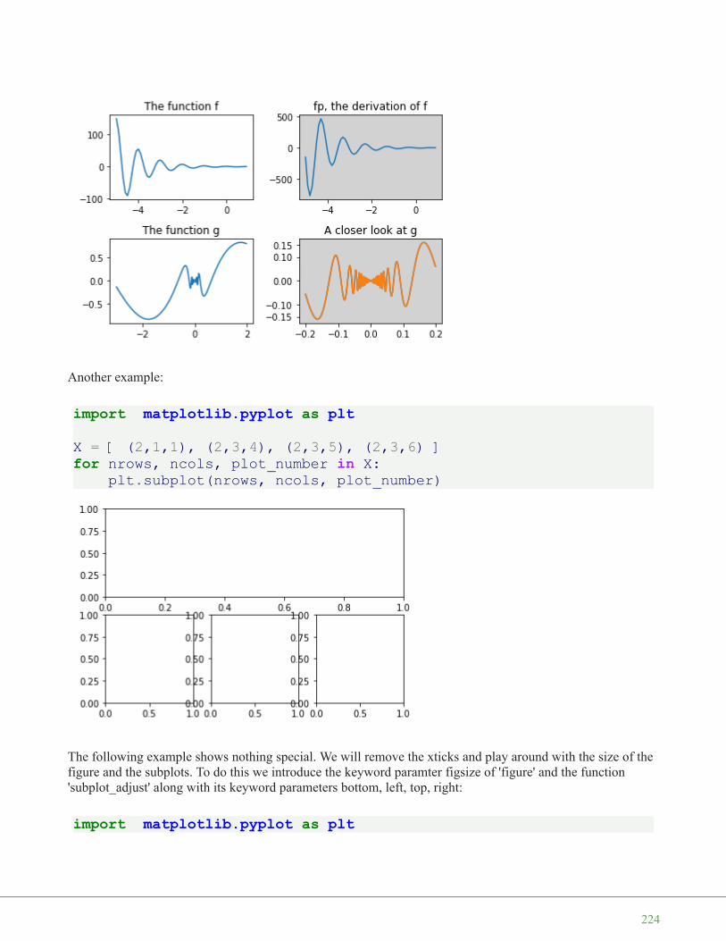
Another example:

import matplotlib.pyplot as pltX = [ (2,1,1), (2,3,4), (2,3,5), (2,3,6) ]for nrows, ncols, plot_number in X:

plt.subplot(nrows, ncols, plot_number)

The following example shows nothing special. We will remove the xticks and play around with the size of thefigure and the subplots. To do this we introduce the keyword paramter figsize of 'figure' and the function'subplot_adjust' along with its keyword parameters bottom, left, top, right:

import matplotlib.pyplot as plt

224

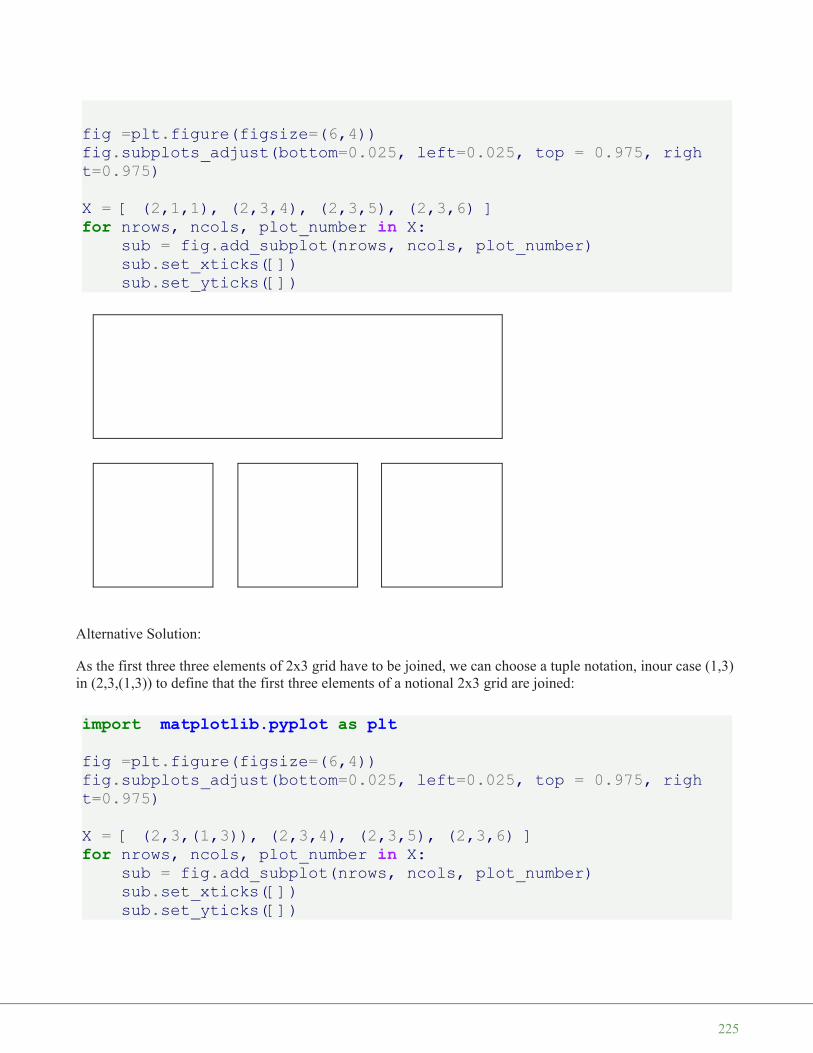
fig =plt.figure(figsize=(6,4))fig.subplots_adjust(bottom=0.025, left=0.025, top = 0.975, right=0.975)

X = [ (2,1,1), (2,3,4), (2,3,5), (2,3,6) ]for nrows, ncols, plot_number in X:

sub = fig.add_subplot(nrows, ncols, plot_number)sub.set_xticks([])sub.set_yticks([])

Alternative Solution:

As the first three three elements of 2x3 grid have to be joined, we can choose a tuple notation, inour case (1,3)in (2,3,(1,3)) to define that the first three elements of a notional 2x3 grid are joined:

import matplotlib.pyplot as pltfig =plt.figure(figsize=(6,4))fig.subplots_adjust(bottom=0.025, left=0.025, top = 0.975, right=0.975)

X = [ (2,3,(1,3)), (2,3,4), (2,3,5), (2,3,6) ]for nrows, ncols, plot_number in X:

sub = fig.add_subplot(nrows, ncols, plot_number)sub.set_xticks([])sub.set_yticks([])

225

226

E X E R C I S E

How can you create a subplotdesign of a 3x2 design, where the complete first column is spanned?

Solution:

import matplotlib.pyplot as pltX = [ (1,2,1), (3,2,2), (3,2,4), (3,2,6) ]for nrows, ncols, plot_number in X:

plt.subplot(nrows, ncols, plot_number)plt.xticks([])plt.yticks([])

227

E X E R C I S E

Create a subplot layout for the following design:

Solution:

import matplotlib.pyplot as pltX = [ (4,2,1),(4,2,2), (4,2,3), (4,2,5), (4,2,(4,6)), (4,1,4)]plt.subplots_adjust(bottom=0, left=0, top = 0.975, right=1)for nrows, ncols, plot_number in X:

plt.subplot(nrows, ncols, plot_number)plt.xticks([])plt.yticks([])

plt.show()

228

SUBPLOTS WITH GRIDSPEC

'matplotlib.gridspec' contains a class GridSpec. It can be used as an alternative to subplot to specify thegeometry of the subplots to be created. The basic idea behind GridSpec is a 'grid'. A grid is set up with anumber of rows and columns. We have to define after this, how much of the grid a subplot should span.

The following example shows the the trivial or simplest case, i.e. a 1x1 grid

import matplotlib.pyplot as pltfrom matplotlib.gridspec import GridSpec

fig = plt.figure()gs = GridSpec(1, 1)ax = fig.add_subplot(gs[0,0])

plt.show()

229

We could have used some of the parameters of Gridspec, e.g. we can define, that our graph should begin at 20% from the bottom and 15 % to the left side of the available figure area:

import matplotlib.pyplot as pltfrom matplotlib.gridspec import GridSpec

fig = plt.figure()gs = GridSpec(1, 1,

bottom=0.2,left=0.15,top=0.8)

ax = fig.add_subplot(gs[0,0])

plt.show()

The next example shows a complexer example with a more elaborate grid design:

230

import matplotlib.gridspec as gridspecimport matplotlib.pyplot as pltplt.figure(figsize=(6, 4))G = gridspec.GridSpec(3, 3)

axes_1 = plt.subplot(G[0, :])axes_1.set_xticks(())axes_1.set_yticks(())axes_1.text(0.5, 0.5, 'Axes 1',

ha='center', va='center',size=24, alpha=.5)

axes_2 = plt.subplot(G[1, :-1])axes_2.set_xticks(())axes_2.set_yticks(())axes_2.text(0.5, 0.5, 'Axes 2',

ha='center', va='center',size=24, alpha=.5)

axes_3 = plt.subplot(G[1:, -1])axes_3.set_xticks(())axes_3.set_yticks(())axes_3.text(0.5, 0.5, 'Axes 3',

ha='center', va='center',size=24, alpha=.5)

axes_4 = plt.subplot(G[-1, 0])axes_4.set_xticks(())axes_4.set_yticks(())axes_4.text(0.5, 0.5, 'Axes 4',

ha='center', va='center',size=24, alpha=.5)

axes_5 = plt.subplot(G[-1, -2])axes_5.set_xticks(())axes_5.set_yticks(())axes_5.text(0.5, 0.5, 'Axes 5',

ha='center', va='center',size=24, alpha=.5)

plt.tight_layout()plt.show()

231

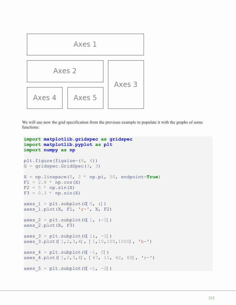
We will use now the grid specification from the previous example to populate it with the graphs of somefunctions:

import matplotlib.gridspec as gridspecimport matplotlib.pyplot as pltimport numpy as npplt.figure(figsize=(6, 4))G = gridspec.GridSpec(3, 3)

X = np.linspace(0, 2 * np.pi, 50, endpoint=True)F1 = 2.8 * np.cos(X)F2 = 5 * np.sin(X)F3 = 0.3 * np.sin(X)

axes_1 = plt.subplot(G[0, :])axes_1.plot(X, F1, 'r-', X, F2)

axes_2 = plt.subplot(G[1, :-1])axes_2.plot(X, F3)

axes_3 = plt.subplot(G[1:, -1])axes_3.plot([1,2,3,4], [1,10,100,1000], 'b-')

axes_4 = plt.subplot(G[-1, 0])axes_4.plot([1,2,3,4], [47, 11, 42, 60], 'r-')

axes_5 = plt.subplot(G[-1, -2])

232

axes_5.plot([1,2,3,4], [7, 5, 4, 3.8])

plt.tight_layout()plt.show()

A PLOT INSIDE OF ANOTHER PLOTimport numpy as npimport matplotlib.pyplot as pltfig = plt.figure()

X = [1, 2, 3, 4, 5, 6, 7]Y = [1, 3, 4, 2, 5, 8, 6]

axes1 = fig.add_axes([0.1, 0.1, 0.9, 0.9]) # main axesaxes2 = fig.add_axes([0.2, 0.6, 0.4, 0.3]) # inset axes

# main figureaxes1.plot(X, Y, 'r')axes1.set_xlabel('x')axes1.set_ylabel('y')axes1.set_title('title')

# insertaxes2.plot(Y, X, 'g')axes2.set_xlabel('y')axes2.set_ylabel('x')axes2.set_title('title inside');

233

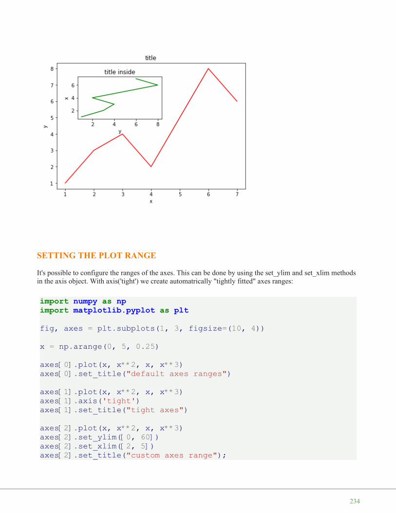
SETTING THE PLOT RANGE

It's possible to configure the ranges of the axes. This can be done by using the set_ylim and set_xlim methodsin the axis object. With axis('tight') we create automatrically "tightly fitted" axes ranges:

import numpy as npimport matplotlib.pyplot as pltfig, axes = plt.subplots(1, 3, figsize=(10, 4))

x = np.arange(0, 5, 0.25)

axes[0].plot(x, x**2, x, x**3)axes[0].set_title("default axes ranges")

axes[1].plot(x, x**2, x, x**3)axes[1].axis('tight')axes[1].set_title("tight axes")

axes[2].plot(x, x**2, x, x**3)axes[2].set_ylim([0, 60])axes[2].set_xlim([2, 5])axes[2].set_title("custom axes range");

234

LOGARITHMIC SCALE

It is also possible to set a logarithmic scale for one or both axes. This functionality is in fact only oneapplication of a more general transformation system in Matplotlib. Each of the axes' scales are set seperatelyusing set_xscale and set_yscale methods which accept one parameter (with the value "log" in this case):

import numpy as npimport matplotlib.pyplot as pltfig = plt.figure()ax = fig.add_subplot(1, 1, 1)

x = np.arange(0, 5, 0.25)

ax.plot(x, x**2, x, x**3)

ax.set_yscale("log")

plt.show()

235

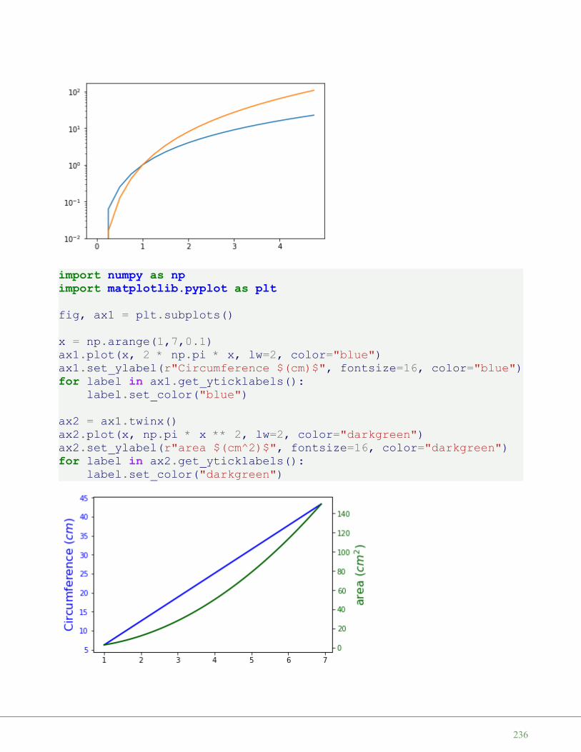
import numpy as npimport matplotlib.pyplot as pltfig, ax1 = plt.subplots()

x = np.arange(1,7,0.1)ax1.plot(x, 2 * np.pi * x, lw=2, color="blue")ax1.set_ylabel(r"Circumference $(cm)$", fontsize=16, color="blue")for label in ax1.get_yticklabels():

label.set_color("blue")

ax2 = ax1.twinx()ax2.plot(x, np.pi * x ** 2, lw=2, color="darkgreen")ax2.set_ylabel(r"area $(cm^2)$", fontsize=16, color="darkgreen")for label in ax2.get_yticklabels():

label.set_color("darkgreen")

236

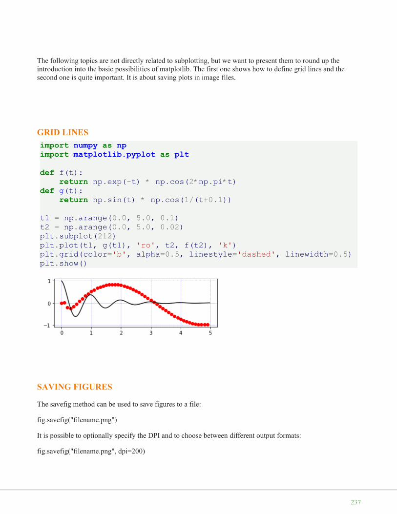
The following topics are not directly related to subplotting, but we want to present them to round up theintroduction into the basic possibilities of matplotlib. The first one shows how to define grid lines and thesecond one is quite important. It is about saving plots in image files.

GRID LINESimport numpy as npimport matplotlib.pyplot as pltdef f(t):

return np.exp(-t) * np.cos(2*np.pi*t)def g(t):

return np.sin(t) * np.cos(1/(t+0.1))

t1 = np.arange(0.0, 5.0, 0.1)t2 = np.arange(0.0, 5.0, 0.02)plt.subplot(212)plt.plot(t1, g(t1), 'ro', t2, f(t2), 'k')plt.grid(color='b', alpha=0.5, linestyle='dashed', linewidth=0.5)plt.show()

SAVING FIGURES

The savefig method can be used to save figures to a file:

fig.savefig("filename.png")

It is possible to optionally specify the DPI and to choose between different output formats:

fig.savefig("filename.png", dpi=200)

237

Output can be generated in the formats PNG, JPG, EPS, SVG, PGF and PDF.

238

M A T P L O T L I B T U T O R I A L : G R I D S P E C

We have seen in the last chapter of ourPython tutorial on Matplotlib how tocreate a figure with multiple axis orsubplot. To create such figures we usedthe subplots function. We willdemonstrate in this chapter how thesubmodule of matplotlib gridspeccan be used to specify the location of thesubplots in a figure. In other words, itspecifies the location of the subplots in agiven GridSpec . GridSpecprovides us with additional control overthe placements of subplots, also the themargins and the spacings between theindividual subplots. It also allows us thecreation of axes which can spread overmultiple grid areas.

We create a figure and four containing axes in the following code. We have covered this in our previouschapter.

import matplotlibimport matplotlib.pyplot as pltimport matplotlib.gridspec as gridspecfig, axes = plt.subplots(ncols=2, nrows=2, constrained_layout=True)

239

We will create the previous example now by using GridSpec. At first, we have to create a figure object andafter this a GridSpec object. We pass the figure object to the parameter figure of GridSpec . The axesare created by using add_subplot . The elements of the gridspec are accessed the same way as numpyarrays.

import matplotlibimport matplotlib.pyplot as pltimport matplotlib.gridspec as gridspecfig = plt.figure(constrained_layout=True)spec = gridspec.GridSpec(ncols=2, nrows=2, figure=fig)ax1 = fig.add_subplot(spec[0, 0])ax2 = fig.add_subplot(spec[0, 1])ax3 = fig.add_subplot(spec[1, 0])ax4 = fig.add_subplot(spec[1, 1])

240

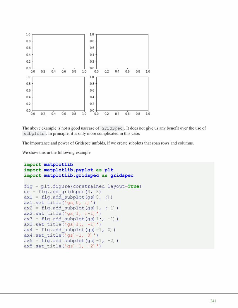
The above example is not a good usecase of GridSpec . It does not give us any benefit over the use ofsubplots . In principle, it is only more complicated in this case.

The importance and power of Gridspec unfolds, if we create subplots that span rows and columns.

We show this in the following example:

import matplotlibimport matplotlib.pyplot as pltimport matplotlib.gridspec as gridspecfig = plt.figure(constrained_layout=True)gs = fig.add_gridspec(3, 3)ax1 = fig.add_subplot(gs[0, :])ax1.set_title('gs[0, :]')ax2 = fig.add_subplot(gs[1, :-1])ax2.set_title('gs[1, :-1]')ax3 = fig.add_subplot(gs[1:, -1])ax3.set_title('gs[1:, -1]')ax4 = fig.add_subplot(gs[-1, 0])ax4.set_title('gs[-1, 0]')ax5 = fig.add_subplot(gs[-1, -2])ax5.set_title('gs[-1, -2]')

241

:mod: ~matplotlib.gridspec is also indispensable for creating subplots of different widths via acouple of methods.

The method shown here is similar to the one above and initializes a uniform grid specification, and then usesnumpy indexing and slices to allocate multiple "cells" for a given subplot.

fig = plt.figure(constrained_layout=True)spec = fig.add_gridspec(ncols=2, nrows=2)optional_params = dict(xy=(0.5, 0.5),

xycoords='axes fraction',va='center',ha='center')

ax = fig.add_subplot(spec[0, 0])ax.annotate('GridSpec[0, 0]', **optional_params)fig.add_subplot(spec[0, 1]).annotate('GridSpec[0, 1:]', **optional_params)fig.add_subplot(spec[1, 0]).annotate('GridSpec[1:, 0]', **optional_params)fig.add_subplot(spec[1, 1]).annotate('GridSpec[1:, 1:]', **optional_params)

Output: Text(0.5, 1.0, 'gs[-1, -2]')

242

Another option is to use the width_ratios and height_ratios parameters. These keywordarguments are lists of numbers. Note that absolute values are meaningless, only their relative ratios matter.That means that width_ratios=[2, 4, 8] is equivalent to width_ratios=[1, 2, 4] withinequally wide figures. For the sake of demonstration, we'll blindly create the axes within for loops since wewon't need them later.

fig5 = plt.figure(constrained_layout=True)widths = [2, 3, 1.5]heights = [1, 3, 2]spec5 = fig5.add_gridspec(ncols=3, nrows=3, width_ratios=widths,

height_ratios=heights)for row in range(3):

for col in range(3):ax = fig5.add_subplot(spec5[row, col])label = 'Width: {}\nHeight: {}'.format(widths[col], height

s[row])ax.annotate(label, (0.1, 0.5), xycoords='axes fraction', v

a='center')

Output: Text(0.5, 0.5, 'GridSpec[1:, 1:]')

243

G r i d S p e c u s i n gS u b p l o t S p e cYou can create GridSpec from the :class: ~matplotlib.gridspec.SubplotSpec , in which case itslayout parameters are set to that of the location of the given SubplotSpec.

Note this is also available from the more verbose .gridspec.GridSpecFromSubplotSpec .

fig10 = plt.figure(constrained_layout=True)gs0 = fig10.add_gridspec(1, 2)

gs00 = gs0[0].subgridspec(2, 3)gs01 = gs0[1].subgridspec(3, 2)

for a in range(2):for b in range(3):

fig10.add_subplot(gs00[a, b])fig10.add_subplot(gs01[b, a])

244

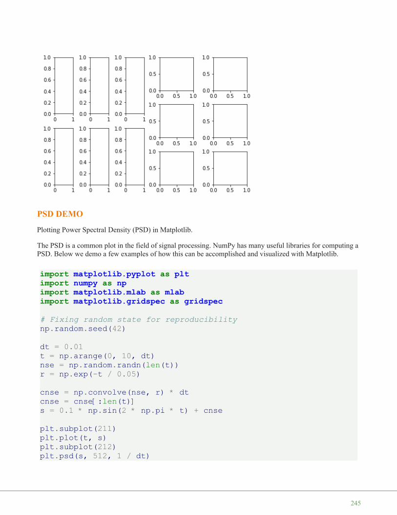
PSD DEMO

Plotting Power Spectral Density (PSD) in Matplotlib.

The PSD is a common plot in the field of signal processing. NumPy has many useful libraries for computing aPSD. Below we demo a few examples of how this can be accomplished and visualized with Matplotlib.

import matplotlib.pyplot as pltimport numpy as npimport matplotlib.mlab as mlabimport matplotlib.gridspec as gridspec# Fixing random state for reproducibilitynp.random.seed(42)

dt = 0.01t = np.arange(0, 10, dt)nse = np.random.randn(len(t))r = np.exp(-t / 0.05)

cnse = np.convolve(nse, r) * dtcnse = cnse[:len(t)]s = 0.1 * np.sin(2 * np.pi * t) + cnse

plt.subplot(211)plt.plot(t, s)plt.subplot(212)plt.psd(s, 512, 1 / dt)

245

plt.show()

This type of flexible grid alignment has a wide range of uses. I most often use it when creating multi-axeshistogram plots like the ones shown here:

# Create some normally distributed datamean = [0, 0]cov = [[1, 1], [1, 2]]x, y = np.random.multivariate_normal(mean, cov, 3000).T

# Set up the axes with gridspecfig = plt.figure(figsize=(6, 6))grid = plt.GridSpec(4, 4, hspace=0.2, wspace=0.2)main_ax = fig.add_subplot(grid[:-1, 1:])y_hist = fig.add_subplot(grid[:-1, 0], xticklabels=[], sharey=main_ax)x_hist = fig.add_subplot(grid[-1, 1:], yticklabels=[], sharex=main_ax)

# scatter points on the main axesmain_ax.plot(x, y, 'ok', markersize=3, alpha=0.2)

# histogram on the attached axesx_hist.hist(x, 40, histtype='stepfilled',

orientation='vertical', color='gray')x_hist.invert_yaxis()

y_hist.hist(y, 40, histtype='stepfilled',

246

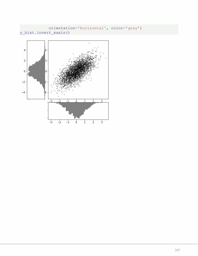
orientation='horizontal', color='gray')y_hist.invert_xaxis()

247

M A T P L O T L I B T U T O R I A L : H I S T O G R A M S A N DB A R P L O T S

It's hard to imagine that you open a newspaper or magazinwithout seeing some bar charts or histograms telling youabout the number of smokers in certain age groups, thenumber of births per year and so on. It's a great way todepict facts without having to use too many words, but onthe downside they can be used to manipulate or lie withstatistics as well. They provide us with quantitativeinformation on a wide range of topics. Bar charts andcolumn charts clearly show us the ranking of our toppoliticians. They also inform about consequences of certainbehavior: smoking or not smoking. Advantages anddisadvantages of various activities. Income distributions and so on. On the one hand, they serve as a source ofinformation for us to see our own thinking and acting in statistical comparison with others, on the other handthey also - by perceiving them - change our thinking and acting in many cases.

However, we are primarily interested in how to create charts and histograms in this chapter. A splendid way tocreate such charts consists in using Python in combination with Matplotlib.

What is a histogram? A formal definition can be: It's a graphical representation of a frequency distribution ofsome numerical data. Rectangles with equal width have heights with the associated frequencies.

If we construct a histogram, we start with distributing the range of possible x values into usually equal sizedand adjacent intervals or bins.

We start now with a practical Python program. We create a histogram with random numbers:

import matplotlib.pyplot as pltimport numpy as npgaussian_numbers = np.random.normal(size=10000)gaussian_numbers

plt.hist(gaussian_numbers)plt.title("Gaussian Histogram")plt.xlabel("Value")plt.ylabel("Frequency")plt.show()

Output: array([-0.80404388, -2.77483865, -2.26510843, ..., -0.6985082 ,

1.21066701, 0.4700107 ])

248

We have seen that the function hist (actually matplotlib.pyplot.hist) computes the histogram values and plotsthe graph. It also returns a tuple of three objects (n, bins, patches):

n, bins, patches = plt.hist(gaussian_numbers)

n[i] contains the number of values of gaussian numbers that lie within the interval with the boundaries bins [i]and bins [i + 1]:

print("n: ", n, sum(n))

So n is an array of frequencies. The last return value of hist is a list of patches, which corresponds to therectangles with their properties:

n: [ 5. 61. 385. 1254. 2728. 3012. 1839. 585. 115. 16.]10000.0

249

print("patches: ", patches)for i in range(10):

print(patches[i])

Let's take a closer look at the return values. To create the histogram array gaussian_numbers are divided intoequal intervals, i.e. the "bins". The interval limits calculated by hist are obtained in the second component ofthe return tuple. In our example, they are denoted by the variable bins:

n, bins, patches = plt.hist(gaussian_numbers)print("n: ", n, sum(n))print("bins: ", bins)for i in range(len(bins)-1):

print(bins[i+1] -bins[i])print("patches: ", patches)print(patches[1])print(patches[2])

patches: <BarContainer object of 10 artists>Rectangle(xy=(-4.08653, 0), width=0.79308, height=5, angle=0)Rectangle(xy=(-3.29345, 0), width=0.79308, height=61, angle=0)Rectangle(xy=(-2.50037, 0), width=0.79308, height=385, angle=0)Rectangle(xy=(-1.70729, 0), width=0.79308, height=1254, angle=0)Rectangle(xy=(-0.914206, 0), width=0.79308, height=2728, angle=0)Rectangle(xy=(-0.121126, 0), width=0.79308, height=3012, angle=0)Rectangle(xy=(0.671954, 0), width=0.79308, height=1839, angle=0)Rectangle(xy=(1.46503, 0), width=0.79308, height=585, angle=0)Rectangle(xy=(2.25811, 0), width=0.79308, height=115, angle=0)Rectangle(xy=(3.05119, 0), width=0.79308, height=16, angle=0)

250

Let's increase the number of bins. 10 bins is not a lot, if you imagine, that we have 10,000 random values. Todo so, we set the keyword parameter bins to 100:

plt.hist(gaussian_numbers, bins=100)plt.show()

n: [ 5. 61. 385. 1254. 2728. 3012. 1839. 585. 115. 16.]10000.0bins: [-4.08652622 -3.29344612 -2.50036601 -1.7072859 -0.9142058 -0.12112569

0.67195442 1.46503452 2.25811463 3.05119474 3.84427484]0.79308010673299910.79308010673299870.79308010673299870.79308010673299910.79308010673299910.79308010673299820.79308010673299910.79308010673299910.79308010673299910.7930801067329982patches: <BarContainer object of 10 artists>Rectangle(xy=(-3.29345, 0), width=0.79308, height=61, angle=0)Rectangle(xy=(-2.50037, 0), width=0.79308, height=385, angle=0)

251

Indem wir den Parameter orientation auf vertical setzen, können wir das Histogramm auch seitwärts ausgeben:

plt.hist(gaussian_numbers,bins=100,orientation="horizontal")

plt.show()

Another important keyword parameter of hist is density, which replaces the deprecated normed parameter. Ifset to true, the first component - that is, the frequencies - of the return tuple is normalized to form a probabilitydensity, i. the area (or the integral) under the histogram makes the sum 1

n, bins, patches = plt.hist(gaussian_numbers,bins=100,density=True)

plt.show()

252

print("Area below the integral: ", np.sum(n * np.diff(bins)))

If both the parameters 'density' and 'stacked' are set to 'True', the sum of the histograms is normalized to 1.With the parameters edgecolor and color we can define the line color and the color of the surfaces:

plt.hist(gaussian_numbers,bins=100,density=True,stacked=True,edgecolor="#6A9662",color="#DDFFDD")

plt.show()

Okay, you want to see the data depicted as a plot of cumulative values? We can plot it as a cumulative

Area below the integral: 1.0

253

distribution function by setting the parameter 'cumulative'.

plt.hist(gaussian_numbers,bins=100,stacked=True,cumulative=True)

plt.show()

BAR PLOTS

Now we come to one of the most commonly used chart types, well known even among non-scientists. A barchart is composed of rectangles that are perpendicular to the x-axis and that rise up like columns. The width ofthe rectangles has no mathematical meaning.

bars = plt.bar([1, 2, 3, 4], [1, 4, 9, 16])bars[0].set_color('green')plt.show()

254

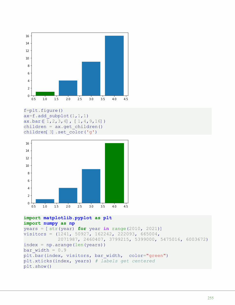
f=plt.figure()ax=f.add_subplot(1,1,1)ax.bar([1,2,3,4], [1,4,9,16])children = ax.get_children()children[3].set_color('g')

import matplotlib.pyplot as pltimport numpy as npyears = [str(year) for year in range(2010, 2021)]visitors = (1241, 50927, 162242, 222093, 665004,

2071987, 2460407, 3799215, 5399000, 5475016, 6003672)index = np.arange(len(years))bar_width = 0.9plt.bar(index, visitors, bar_width, color="green")plt.xticks(index, years) # labels get centeredplt.show()

255

BARPLOTS WITH CUSTOMIZED TICKSfrom matplotlib.ticker import FuncFormatterimport matplotlib.pyplot as pltimport numpy as npdef millions(x, pos):

'The two args are the value and tick position'#return '$%1.1fM' % (x * 1e-6)return f'${x * 1e-6:1.1f}M'

formatter = FuncFormatter(millions)

years = ('US', 'EU', 'China', 'Japan','Germany', 'UK', 'France', 'India')

GDP = (20494050, 18750052, 13407398, 4971929,4000386, 2828644, 2775252, 2716746)

fig, ax = plt.subplots()ax.yaxis.set_major_formatter(formatter)ax.bar(x=np.arange(len(GDP)), # The x coordinates of the bars.

height=GDP, # the height(s) of the varscolor="green",align="center",tick_label=years)

ax.set_ylabel('GDP in $')ax.set_title('Largest Economies by nominal GDP in 2018')plt.show()

256

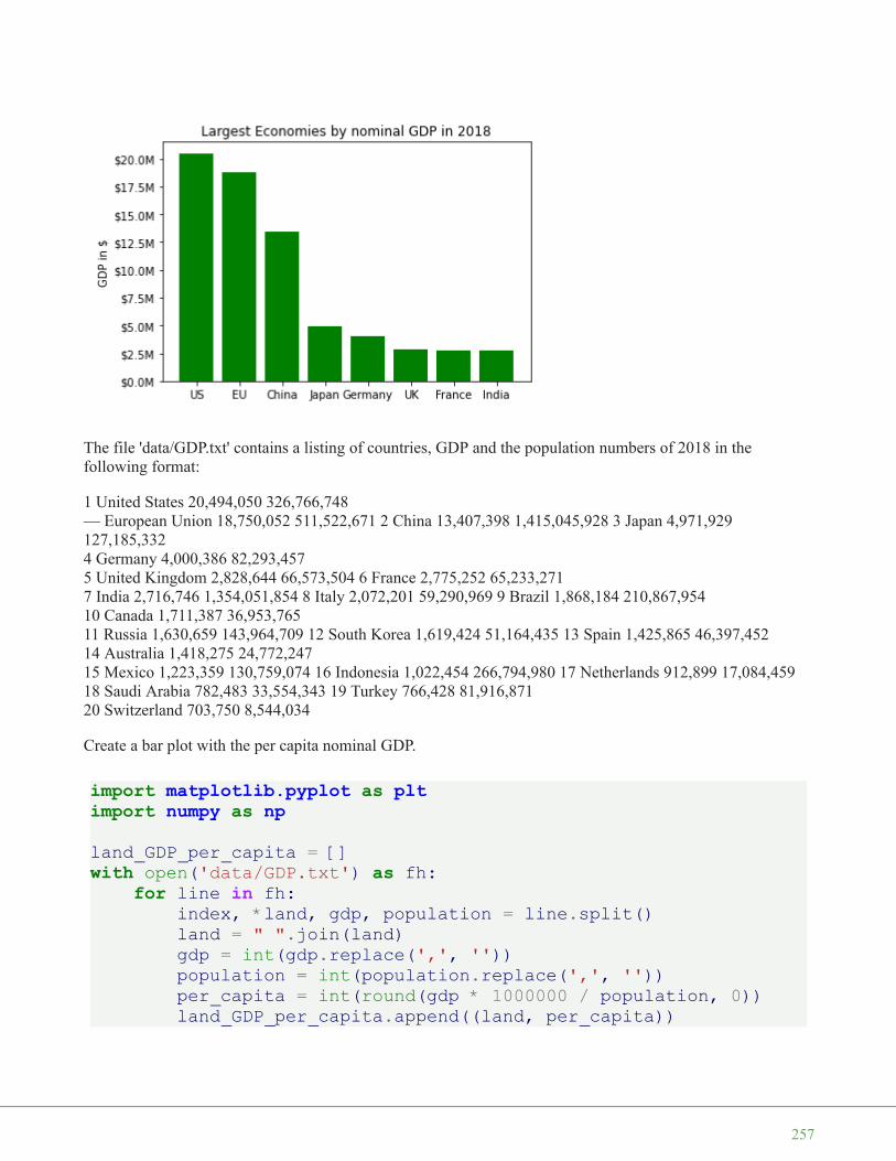
The file 'data/GDP.txt' contains a listing of countries, GDP and the population numbers of 2018 in thefollowing format:

1 United States 20,494,050 326,766,748— European Union 18,750,052 511,522,671 2 China 13,407,398 1,415,045,928 3 Japan 4,971,929127,185,3324 Germany 4,000,386 82,293,4575 United Kingdom 2,828,644 66,573,504 6 France 2,775,252 65,233,2717 India 2,716,746 1,354,051,854 8 Italy 2,072,201 59,290,969 9 Brazil 1,868,184 210,867,95410 Canada 1,711,387 36,953,76511 Russia 1,630,659 143,964,709 12 South Korea 1,619,424 51,164,435 13 Spain 1,425,865 46,397,45214 Australia 1,418,275 24,772,24715 Mexico 1,223,359 130,759,074 16 Indonesia 1,022,454 266,794,980 17 Netherlands 912,899 17,084,45918 Saudi Arabia 782,483 33,554,343 19 Turkey 766,428 81,916,87120 Switzerland 703,750 8,544,034

Create a bar plot with the per capita nominal GDP.

import matplotlib.pyplot as pltimport numpy as npland_GDP_per_capita = []with open('data/GDP.txt') as fh:

for line in fh:index, *land, gdp, population = line.split()land = " ".join(land)gdp = int(gdp.replace(',', ''))population = int(population.replace(',', ''))per_capita = int(round(gdp * 1000000 / population, 0))land_GDP_per_capita.append((land, per_capita))

257

land_GDP_per_capita.sort(key=lambda x: x[1], reverse=True)countries, GDP_per_capita = zip(*land_GDP_per_capita)

fig = plt.figure(figsize=(6,5), dpi=200)left, bottom, width, height = 0.1, 0.3, 0.8, 0.6ax = fig.add_axes([left, bottom, width, height])

ax.bar(x=np.arange(len(GDP_per_capita)), # The x coordinates of the bars.

height=GDP_per_capita, # the height(s) of the varscolor="green", align="center",tick_label=countries)

ax.set_ylabel('in thousands of $')#ax.set_xticks(rotation='vertical')ax.set_title('Largest Economies by nominal GDP in 2018')plt.xticks(rotation=90)plt.show()

258

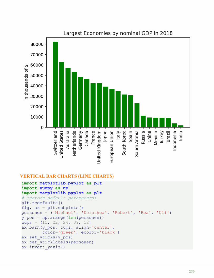
VERTICAL BAR CHARTS (LINE CHARTS)import matplotlib.pyplot as pltimport numpy as npimport matplotlib.pyplot as plt# restore default parameters:plt.rcdefaults()fig, ax = plt.subplots()personen = ('Michael', 'Dorothea', 'Robert', 'Bea', 'Uli')y_pos = np.arange(len(personen))cups = (15, 22, 24, 39, 12)ax.barh(y_pos, cups, align='center',

color='green', ecolor='black')ax.set_yticks(y_pos)ax.set_yticklabels(personen)ax.invert_yaxis()

259

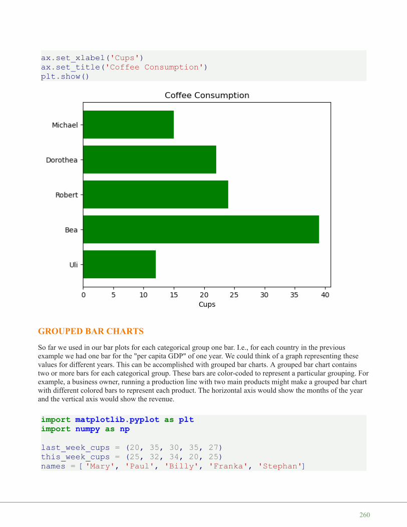
ax.set_xlabel('Cups')ax.set_title('Coffee Consumption')plt.show()

GROUPED BAR CHARTS

So far we used in our bar plots for each categorical group one bar. I.e., for each country in the previousexample we had one bar for the "per capita GDP" of one year. We could think of a graph representing thesevalues for different years. This can be accomplished with grouped bar charts. A grouped bar chart containstwo or more bars for each categorical group. These bars are color-coded to represent a particular grouping. Forexample, a business owner, running a production line with two main products might make a grouped bar chartwith different colored bars to represent each product. The horizontal axis would show the months of the yearand the vertical axis would show the revenue.

import matplotlib.pyplot as pltimport numpy as nplast_week_cups = (20, 35, 30, 35, 27)this_week_cups = (25, 32, 34, 20, 25)names = ['Mary', 'Paul', 'Billy', 'Franka', 'Stephan']

260

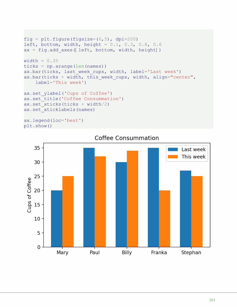
fig = plt.figure(figsize=(6,5), dpi=200)left, bottom, width, height = 0.1, 0.3, 0.8, 0.6ax = fig.add_axes([left, bottom, width, height])

width = 0.35ticks = np.arange(len(names))ax.bar(ticks, last_week_cups, width, label='Last week')ax.bar(ticks + width, this_week_cups, width, align="center",

label='This week')

ax.set_ylabel('Cups of Coffee')ax.set_title('Coffee Consummation')ax.set_xticks(ticks + width/2)ax.set_xticklabels(names)

ax.legend(loc='best')plt.show()

261

EXERCISE

The file data/german_election_results.txt contains four election result of Germany.

Create a bar chart graph with data.

import matplotlib.pyplot as pltimport numpy as npparties = ('CDU/CSU', 'SPD', 'FDP', 'Grüne', 'Die Linke', 'AfD')

election_results_per_year = {}with open('data/german_election_results.txt') as fh:

fh.readline()for line in fh:

year, *results = line.rsplit()election_results_per_year[year] = [float(x) for x in resul

ts]

election_results_per_party = list(zip(*election_results_per_year.values()))

fig = plt.figure(figsize=(6,5), dpi=200)left, bottom, width, height = 0.1, 0.1, 0.8, 0.8ax = fig.add_axes([left, bottom, width, height])

years = list(election_results_per_year.keys())width = 0.9 / len(parties)ticks = np.arange(len(years))

for index, party in enumerate(parties):ax.bar(ticks+index*width, election_results_per_party[index], w

idth, label=party)

ax.set_ylabel('Percentages of Votes')ax.set_title('German Elections')ax.set_xticks(ticks + 0.45)ax.set_xticklabels(years)

ax.legend(loc='best')plt.show()

262

We change the previous code by adding the following dictionary:

colors = {'CDU/CSU': "black", 'SPD': "r", 'FDP': "y",'Grüne': "green", 'Die Linke': "purple", 'AfD': "blue"}

We also change the creation of the bar code by assigning a color value to the parameter ‚color‘:

for index, party in enumerate(parties):ax.bar(ticks+index*width,

election_results_per_party[index],width,label=party,color=colors[parties[index]])

263

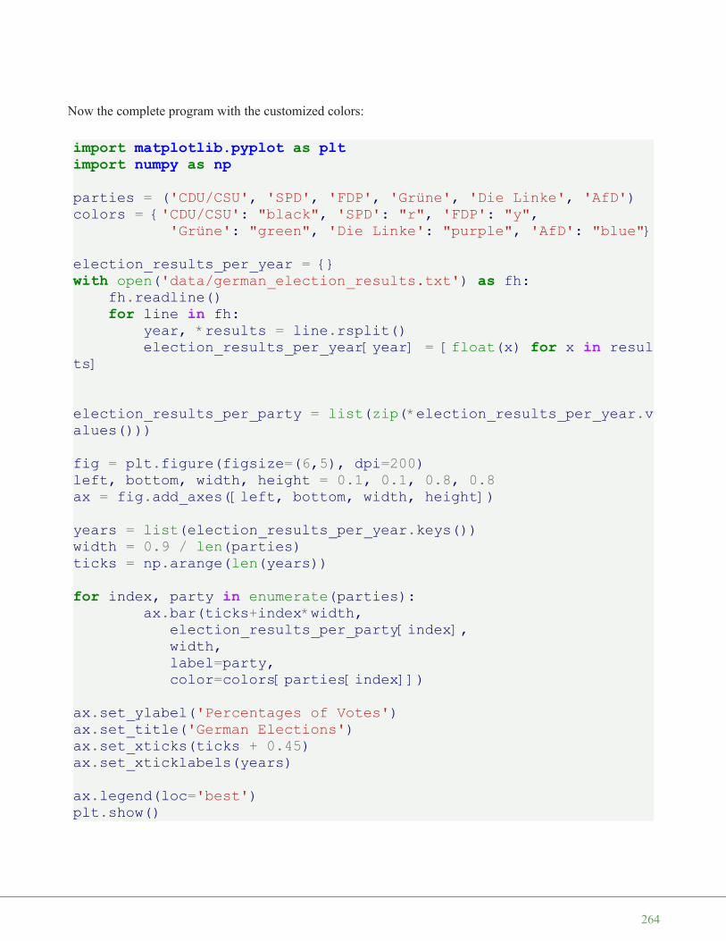
Now the complete program with the customized colors:

import matplotlib.pyplot as pltimport numpy as npparties = ('CDU/CSU', 'SPD', 'FDP', 'Grüne', 'Die Linke', 'AfD')colors = {'CDU/CSU': "black", 'SPD': "r", 'FDP': "y",

'Grüne': "green", 'Die Linke': "purple", 'AfD': "blue"}

election_results_per_year = {}with open('data/german_election_results.txt') as fh:

fh.readline()for line in fh:

year, *results = line.rsplit()election_results_per_year[year] = [float(x) for x in resul

ts]

election_results_per_party = list(zip(*election_results_per_year.values()))

fig = plt.figure(figsize=(6,5), dpi=200)left, bottom, width, height = 0.1, 0.1, 0.8, 0.8ax = fig.add_axes([left, bottom, width, height])

years = list(election_results_per_year.keys())width = 0.9 / len(parties)ticks = np.arange(len(years))

for index, party in enumerate(parties):ax.bar(ticks+index*width,

election_results_per_party[index],width,label=party,color=colors[parties[index]])

ax.set_ylabel('Percentages of Votes')ax.set_title('German Elections')ax.set_xticks(ticks + 0.45)ax.set_xticklabels(years)

ax.legend(loc='best')plt.show()

264

STACKED BAR CHARS

As an alternative to grouped bar charts stacked bar charts can be used.

The stacked bar chart stacks bars that represent different groups on top of each other. The height of theresulting bar shows the combined result or summation of the individual groups.

Stacked bar charts are great to depict the total and at the same time providing a view of how the single partsare related to the sum.

Stacked bar charts are not suited for datasets where some groups have negative values. In such cases, groupedbar charts are the better choice.

import matplotlib.pyplot as plt

265

import numpy as npcoffee = np.array([5, 5, 7, 6, 7])tea = np.array([1, 2, 0, 2, 0])water = np.array([10, 12, 14, 12, 15])names = ['Mary', 'Paul', 'Billy', 'Franka', 'Stephan']

fig = plt.figure(figsize=(6,5), dpi=200)left, bottom, width, height = 0.2, 0.1, 0.7, 0.8ax = fig.add_axes([left, bottom, width, height])

width = 0.35ticks = np.arange(len(names))ax.bar(ticks, tea, width, label='Coffee', bottom=water+coffee)ax.bar(ticks, coffee, width, align="center", label='Tea',

bottom=water)ax.bar(ticks, water, width, align="center", label='Water')

266

Output: <BarContainer object of 5 artists>

267

M A T P L O T L I B T U T O R I A L : C O N T O U R P L O T S

CONTOUR PLOT

A contour line or isoline of a function of two variables is acurve along which the function has a constant value.

It is a cross-section of the three-dimensional graph of thefunction f(x, y) parallel to the x, y plane.

Contour lines are used e.g. in geography and meteorology.

In cartography, a contour line joins points of equal elevation(height) above a given level, such as mean sea level.

We can also say in a more general way that a contour line ofa function with two variables is a curve which connects points with the same values.

CREATING A "MESHGRID"

268

# the following line is only necessary if working with "ipython notebook"%matplotlib inline

import matplotlib.pyplot as pltimport numpy as npn, m = 7, 7start = -3

x_vals = np.arange(start, start+n, 1)y_vals = np.arange(start, start+m, 1)X, Y = np.meshgrid(x_vals, y_vals)

print(X)print(Y)

269

We can visulize our meshgridif we add the following code to our previous program:

fig, ax = plt.subplots()

ax.scatter(X, Y, color="green")ax.set_title('Regular Grid, created by Meshgrid')ax.set_xlabel('x')ax.set_ylabel('y')plt.show()

import numpy as npxlist = np.linspace(-3.0, 3.0, 3)ylist = np.linspace(-3.0, 3.0, 4)

[[-3 -2 -1 0 1 2 3][-3 -2 -1 0 1 2 3][-3 -2 -1 0 1 2 3][-3 -2 -1 0 1 2 3][-3 -2 -1 0 1 2 3][-3 -2 -1 0 1 2 3][-3 -2 -1 0 1 2 3]]

[[-3 -3 -3 -3 -3 -3 -3][-2 -2 -2 -2 -2 -2 -2][-1 -1 -1 -1 -1 -1 -1][ 0 0 0 0 0 0 0][ 1 1 1 1 1 1 1][ 2 2 2 2 2 2 2][ 3 3 3 3 3 3 3]]

270

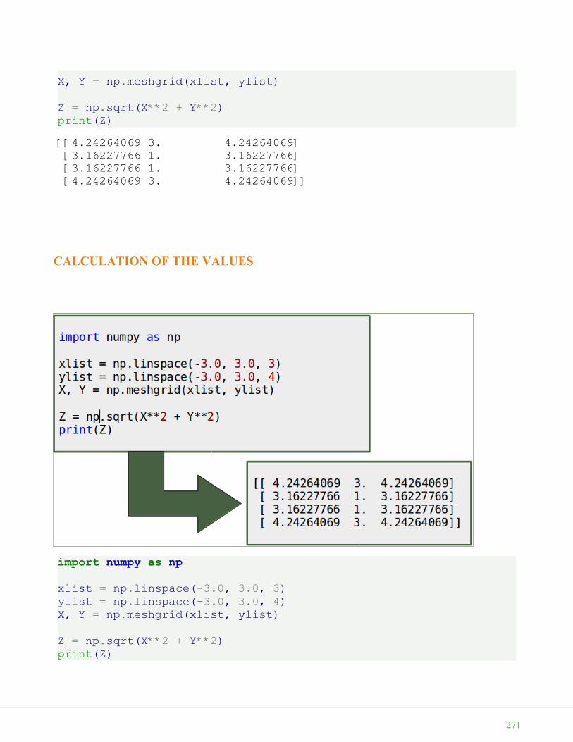
X, Y = np.meshgrid(xlist, ylist)

Z = np.sqrt(X**2 + Y**2)print(Z)

CALCULATION OF THE VALUES

import numpy as npxlist = np.linspace(-3.0, 3.0, 3)ylist = np.linspace(-3.0, 3.0, 4)X, Y = np.meshgrid(xlist, ylist)

Z = np.sqrt(X**2 + Y**2)print(Z)

[[4.24264069 3. 4.24264069][3.16227766 1. 3.16227766][3.16227766 1. 3.16227766][4.24264069 3. 4.24264069]]

271

fig = plt.figure(figsize=(6,5))left, bottom, width, height = 0.1, 0.1, 0.8, 0.8ax = fig.add_axes([left, bottom, width, height])

Z = np.sqrt(X**2 + Y**2)cp = ax.contour(X, Y, Z)ax.clabel(cp, inline=True,

fontsize=10)ax.set_title('Contour Plot')ax.set_xlabel('x (cm)')ax.set_ylabel('y (cm)')plt.show()

CHANGING THE COLOURS AND THE LINE STYLEimport matplotlib.pyplot as plt

[[4.24264069 3. 4.24264069][3.16227766 1. 3.16227766][3.16227766 1. 3.16227766][4.24264069 3. 4.24264069]]

272

plt.figure()cp = plt.contour(X, Y, Z, colors='black', linestyles='dashed')plt.clabel(cp, inline=True,

fontsize=10)plt.title('Contour Plot')plt.xlabel('x (cm)')plt.ylabel('y (cm)')plt.show()

FILLED CONTOURSimport matplotlib.pyplot as pltimport numpy as npfig = plt.figure(figsize=(6,5))left, bottom, width, height = 0.1, 0.1, 0.8, 0.8ax = fig.add_axes([left, bottom, width, height])

start, stop, n_values = -8, 8, 800

x_vals = np.linspace(start, stop, n_values)y_vals = np.linspace(start, stop, n_values)X, Y = np.meshgrid(x_vals, y_vals)

273

Z = np.sqrt(X**2 + Y**2)

cp = plt.contourf(X, Y, Z)plt.colorbar(cp)

ax.set_title('Contour Plot')ax.set_xlabel('x (cm)')ax.set_ylabel('y (cm)')plt.show()

INDIVIDUAL COLOURSimport numpy as npimport matplotlib.pyplot as pltxlist = np.linspace(-3.0, 3.0, 100)ylist = np.linspace(-3.0, 3.0, 100)X, Y = np.meshgrid(xlist, ylist)Z = np.sqrt(X**2 + Y**2)

plt.figure()

274

contour = plt.contour(X, Y, Z)plt.clabel(contour, colors = 'k', fmt = '%2.1f', fontsize=12)c = ('#ff0000', '#ffff00', '#0000FF', '0.6', 'c', 'm')contour_filled = plt.contourf(X, Y, Z, colors=c)plt.colorbar(contour_filled)

plt.title('Filled Contours Plot')plt.xlabel('x (cm)')plt.ylabel('y (cm)')plt.savefig('contourplot_own_colours.png', dpi=300)plt.show()

LEVELS

The levels were decided automatically by contour and contourf so far. They can be defined manually, byproviding a list of levels as a fourth parameter. Contour lines will be drawn for each value in the list, if we usecontour. For contourf, there will be filled colored regions between the values in the list.

In [ ]:

import numpy as npimport matplotlib.pyplot as pltxlist = np.linspace(-3.0, 3.0, 100)ylist = np.linspace(-3.0, 3.0, 100)

275

X, Y = np.meshgrid(xlist, ylist)

Z = np.sqrt(X ** 2 + Y ** 2 )plt.figure()

levels = [0.0, 0.2, 0.5, 0.9, 1.5, 2.5, 3.5]contour = plt.contour(X, Y, Z, levels, colors='k')plt.clabel(contour, colors = 'k', fmt = '%2.1f', fontsize=12)contour_filled = plt.contourf(X, Y, Z, levels)plt.colorbar(contour_filled)

plt.title('Plot from level list')plt.xlabel('x (cm)')plt.ylabel('y (cm)')plt.show()

The last example of this chapter will be a "lovely" contour plot:

In [ ]:

import matplotlib.pyplot as pltimport numpy as npy, x = np.ogrid[-1:2:100j, -1:1:100j]plt.contour(x.ravel(),

y.ravel(),x**2 + (y-((x**2)**(1.0/3)))**2,[1],colors='red',)

plt.axis('equal')plt.show()

In [ ]:

276

I M A G E P R O C E S S I N G

INTRODUCTION

It has never been easier to take a picture than it istoday. All you normally need is a cell phone. Theseare the essentials to take and view a picture. Takingphotos is free if we don't include the cost of themobile phone, which is often bought for otherpurposes anyway. A generation ago, amateur and realartists needed specialized and often expensiveequipment, and the cost per image was far from free.

We take photos to preserve great moments of our lifein time. "Pickled memories" ready to be "opened" inthe future at will.

Similar to pickling, we need to use the rightpreservatives. Of course, the mobile phone alsooffers us a range of image processing software, but assoon as we have to process a large amount of photos,we need other tools. This is when programming andPython come into play. Python and its modules suchas Numpy, Scipy, Matplotlib and other specialmodules offer the optimal functionality to cope withthe flood of images.

In order to provide you with the necessary knowledge, this chapter of our Python tutorial deals with basicimage processing and manipulation. For this purpose we use the modules NumPy, Matplotlib and SciPy.

We start with the scipy package misc . The helpfile says that scipy.misc contains "various utilities thatdon't have another home". For example, it also contains a few images, such as the following:

from scipy import miscimport matplotlib.pyplot as pltascent = misc.ascent()plt.gray()plt.imshow(ascent)plt.show()

277

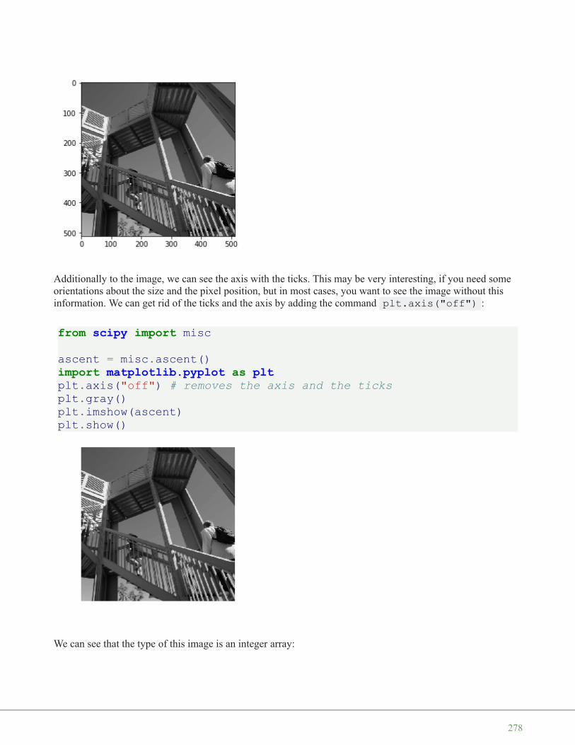
Additionally to the image, we can see the axis with the ticks. This may be very interesting, if you need someorientations about the size and the pixel position, but in most cases, you want to see the image without thisinformation. We can get rid of the ticks and the axis by adding the command plt.axis("off") :

from scipy import misc

ascent = misc.ascent()import matplotlib.pyplot as pltplt.axis("off") # removes the axis and the ticksplt.gray()plt.imshow(ascent)plt.show()

We can see that the type of this image is an integer array:

278

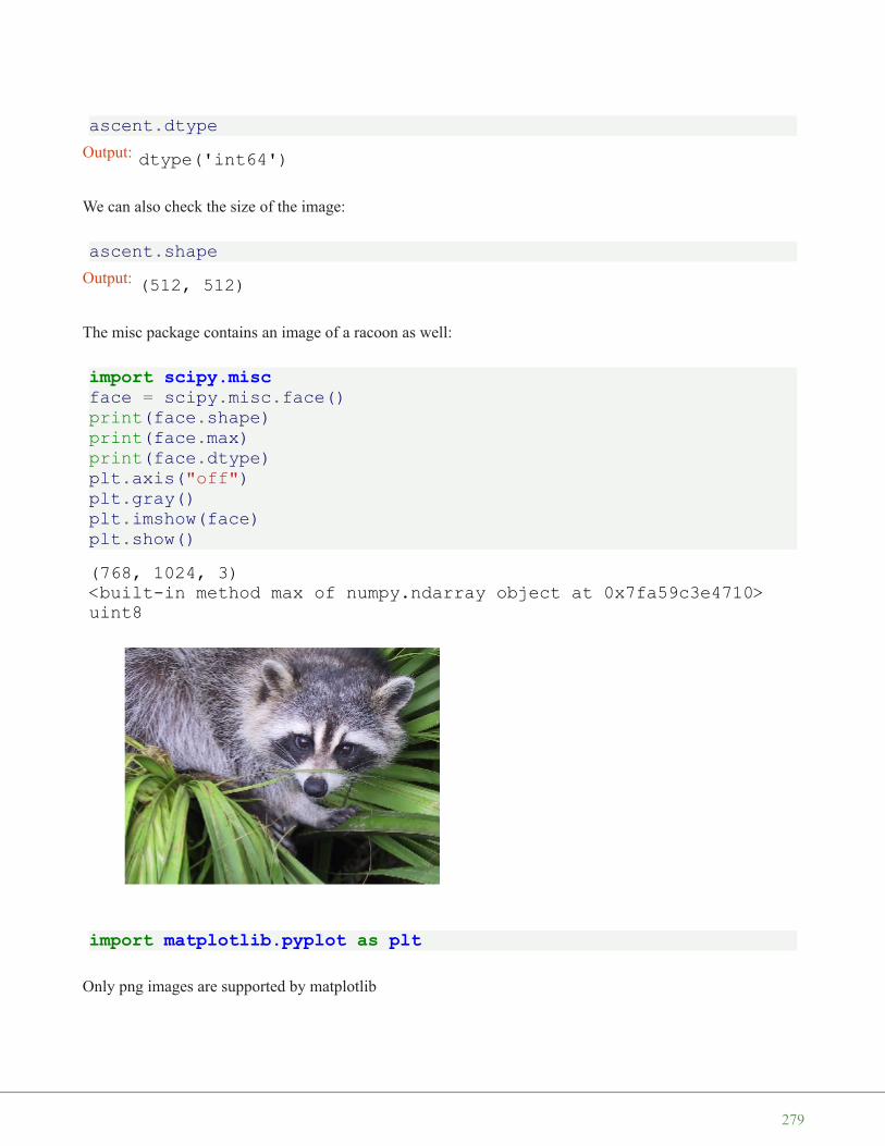
ascent.dtype

We can also check the size of the image:

ascent.shape

The misc package contains an image of a racoon as well:

import scipy.miscface = scipy.misc.face()print(face.shape)print(face.max)print(face.dtype)plt.axis("off")plt.gray()plt.imshow(face)plt.show()

import matplotlib.pyplot as plt

Only png images are supported by matplotlib

Output: dtype('int64')

Output: (512, 512)

(768, 1024, 3)<built-in method max of numpy.ndarray object at 0x7fa59c3e4710>uint8

279

img = plt.imread('frankfurt.png')print(img[:3])

plt.axis("off")imgplot = plt.imshow(img)

lum_img = img[:,:,1]

[[[0.4117647 0.5686275 0.8 ][0.40392157 0.56078434 0.7921569 ][0.40392157 0.5686275 0.79607844]...[0.48235294 0.62352943 0.81960785][0.47843137 0.627451 0.81960785][0.47843137 0.62352943 0.827451 ]]

[[0.40784314 0.5647059 0.79607844][0.40392157 0.56078434 0.7921569 ][0.40392157 0.5686275 0.79607844]...[0.48235294 0.62352943 0.81960785][0.47843137 0.627451 0.81960785][0.48235294 0.627451 0.83137256]]

[[0.40392157 0.5686275 0.79607844][0.40392157 0.5686275 0.79607844][0.40392157 0.5686275 0.79607844]...[0.48235294 0.62352943 0.81960785][0.48235294 0.62352943 0.81960785][0.4862745 0.627451 0.83137256]]]

280

print(lum_img)

plt.axis("off")imgplot = plt.imshow(lum_img)

TINT, SHADE AND TONE

Now, we will show how to tint an image. Tint is an expression from colour theory and an often used techniqueby painters. Thinking about painters and not think about the Netherlands is hard to imagine. So we will use apicture with Dutch windmills in our next example. (The image has been taken at Kinderdijk, a village in theNetherlands, about 15 km east of Rotterdam and about 50 kilometres from Den Haag (The Hague). It's aUNESCO World Heritage Site since 1997.)

windmills = plt.imread('windmills.png')

[[0.5686275 0.56078434 0.5686275 ... 0.62352943 0.627451 0.62352943][0.5647059 0.56078434 0.5686275 ... 0.62352943 0.627451 0.627

451 ][0.5686275 0.5686275 0.5686275 ... 0.62352943 0.62352943 0.627

451 ]...[0.31764707 0.32941177 0.32941177 ... 0.30588236 0.3137255 0.317

64707][0.31764707 0.3137255 0.32941177 ... 0.3019608 0.32156864 0.337

2549 ][0.31764707 0.3019608 0.33333334 ... 0.30588236 0.32156864 0.333

33334]]

281

plt.axis("off")plt.imshow(windmills)

We want to tint the image now. This means we will "mix" our colours with white. This will increase thelightness of our image. For this purpose, we write a Python function, which takes an image and a percentagevalue as a parameter. Setting 'percentage' to 0 will not change the image, setting it to one means that the imagewill be completely whitened:

import numpy as npimport matplotlib.pyplot as pltdef tint(imag, percent):

"""imag: the image which will be shadedpercent: a value between 0 (image will remain unchanged

and 1 (image will completely white)"""tinted_imag = imag + (np.ones(imag.shape) - imag) * percentreturn tinted_imag

windmills = plt.imread('windmills.png')

tinted_windmills = tint(windmills, 0.8)plt.axis("off")plt.imshow(tinted_windmills)

Output: <matplotlib.image.AxesImage at 0x7fa59c2479d0>

282

A shade is the mixture of a color with black, which reduces lightness.

import numpy as npimport matplotlib.pyplot as plt

def shade(imag, percent):"""imag: the image which will be shadedpercent: a value between 0 (image will remain unchanged

and 1 (image will be blackened)"""tinted_imag = imag * (1 - percent)return tinted_imag

windmills = plt.imread('windmills.png')

tinted_windmills = shade(windmills, 0.7)plt.imshow(tinted_windmills)

Output: <matplotlib.image.AxesImage at 0x7fa59c30f350>

283

def vertical_gradient_line(image, reverse=False):"""We create a horizontal gradient line with the shape (1, imag

e.shape[1], 3))The values are incremented from 0 to 1, if reverse is False,otherwise the values are decremented from 1 to 0."""number_of_columns = image.shape[1]if reverse:

C = np.linspace(1, 0, number_of_columns)else:

C = np.linspace(0, 1, number_of_columns)C = np.dstack((C, C, C))return C

horizontal_brush = vertical_gradient_line(windmills)tinted_windmills = windmills * horizontal_brushplt.axis("off")plt.imshow(tinted_windmills)

Output: <matplotlib.image.AxesImage at 0x7fa59c3b8050>

284

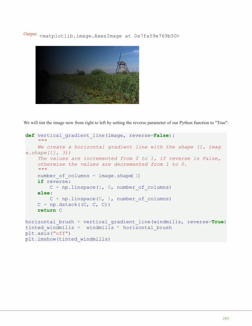
We will tint the image now from right to left by setting the reverse parameter of our Python function to "True":

def vertical_gradient_line(image, reverse=False):"""We create a horizontal gradient line with the shape (1, imag

e.shape[1], 3))The values are incremented from 0 to 1, if reverse is False,otherwise the values are decremented from 1 to 0."""number_of_columns = image.shape[1]if reverse:

C = np.linspace(1, 0, number_of_columns)else:

C = np.linspace(0, 1, number_of_columns)C = np.dstack((C, C, C))return C

horizontal_brush = vertical_gradient_line(windmills, reverse=True)tinted_windmills = windmills * horizontal_brushplt.axis("off")plt.imshow(tinted_windmills)

Output: <matplotlib.image.AxesImage at 0x7fa59e769b50>

285

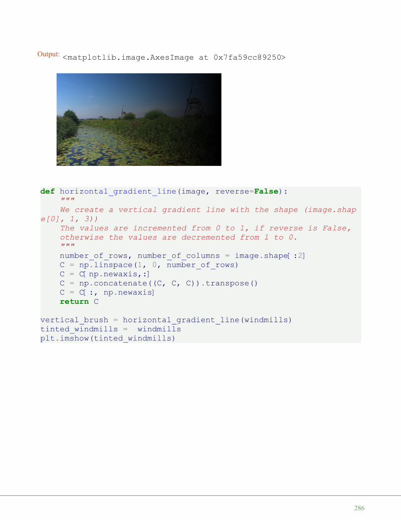
def horizontal_gradient_line(image, reverse=False):"""We create a vertical gradient line with the shape (image.shap

e[0], 1, 3))The values are incremented from 0 to 1, if reverse is False,otherwise the values are decremented from 1 to 0."""number_of_rows, number_of_columns = image.shape[:2]C = np.linspace(1, 0, number_of_rows)C = C[np.newaxis,:]C = np.concatenate((C, C, C)).transpose()C = C[:, np.newaxis]return C

vertical_brush = horizontal_gradient_line(windmills)tinted_windmills = windmillsplt.imshow(tinted_windmills)

Output: <matplotlib.image.AxesImage at 0x7fa59cc89250>

286

A tone is produced either by the mixture of a color with gray, or by both tinting and shading.

charlie = plt.imread('Chaplin.png')plt.gray()print(charlie)plt.imshow(charlie)

Output: <matplotlib.image.AxesImage at 0x7fa59c227dd0>

287

colored = np.dstack((charlie*0.1, charlie*1, charlie*0.5))

plt.imshow(colored)

[[0.16470589 0.16862746 0.1764706 ... 0. 0.0. ][0.16078432 0.16078432 0.16470589 ... 0. 0.

0. ][0.15686275 0.15686275 0.16078432 ... 0. 0.

0. ]...[0. 0. 0. ... 0. 0.

0. ][0. 0. 0. ... 0. 0.

0. ][0. 0. 0. ... 0. 0.

0. ]]Output: <matplotlib.image.AxesImage at 0x7fa59c18f810>

288

tinting gray scale images: http://scikit-image.org/docs/dev/auto_examples/plot_tinting_grayscale_images.html

We will use different colormaps in the following example. The colormaps can be found inmatplotlib.pyplot.cm.datad:

plt.cm.datad.keys()

Output: <matplotlib.image.AxesImage at 0x7fa59c0f9890>

289

import numpy as npimport matplotlib.pyplot as pltcharlie = plt.imread('Chaplin.png')

# colormaps plt.cm.datad# cmaps = set(plt.cm.datad.keys())cmaps = {'afmhot', 'autumn', 'bone', 'binary', 'bwr', 'brg',

'CMRmap', 'cool', 'copper', 'cubehelix', 'Greens'}

X = [(4, 3, 1, (1, 0, 0)),(4, 3, 2, (0.5, 0.5, 0)),(4, 3, 3, (0, 1, 0)),(4, 3, 4, (0, 0.5, 0.5)),(4, 3, (5, 8), (0, 0, 1)),(4, 3, 6, (1, 1, 0)),

Output: dict_keys(['Blues', 'BrBG', 'BuGn', 'BuPu', 'CMRmap', 'GnBu', 'Greens', 'Greys', 'OrRd', 'Oranges', 'PRGn', 'PiYG', 'PuBu', 'PuBuGn', 'PuOr', 'PuRd', 'Purples', 'RdBu', 'RdGy', 'RdPu', 'RdYlBu', 'RdYlGn', 'Reds', 'Spectral', 'Wistia', 'YlGn', 'YlGnBu', 'YlOrBr', 'YlOrRd', 'afmhot', 'autumn', 'binary', 'bone', 'brg', 'bwr', 'cool', 'coolwarm', 'copper', 'cubehelix', 'flag', 'gist_earth', 'gist_gray', 'gist_heat', 'gist_ncar', 'gist_rainbow', 'gist_stern', 'gist_yarg', 'gnuplot', 'gnuplot2', 'gray', 'hot', 'hsv', 'jet', 'nipy_spectral', 'ocean', 'pink', 'prism', 'rainbow', 'seismic', 'spring', 'summer', 'terrain', 'winter', 'Accent', 'Dark2', 'Paired', 'Pastel1', 'Pastel2', 'Set1', 'Set2', 'Set3', 'tab10', 'tab20', 'tab20b', 'tab20c', 'Blues_r', 'BrBG_r', 'BuGn_r', 'BuPu_r', 'CMRmap_r', 'GnBu_r', 'Greens_r', 'Greys_r', 'OrRd_r', 'Oranges_r', 'PRGn_r', 'PiYG_r', 'PuBu_r', 'PuBuGn_r','PuOr_r', 'PuRd_r', 'Purples_r', 'RdBu_r', 'RdGy_r', 'RdPu_r', 'RdYlBu_r', 'RdYlGn_r', 'Reds_r', 'Spectral_r', 'Wistia_r', 'YlGn_r', 'YlGnBu_r', 'YlOrBr_r', 'YlOrRd_r', 'afmhot_r', 'autumn_r', 'binary_r', 'bone_r', 'brg_r', 'bwr_r', 'cool_r', 'coolwarm_r', 'copper_r', 'cubehelix_r', 'flag_r', 'gist_earth_r', 'gist_gray_r', 'gist_heat_r', 'gist_ncar_r', 'gist_rainbow_r', 'gist_stern_r', 'gist_yarg_r', 'gnuplot_r', 'gnuplot2_r', 'gray_r', 'hot_r', 'hsv_r', 'jet_r', 'nipy_spectral_r', 'ocean_r', 'pink_r', 'prism_r', 'rainbow_r', 'seismic_r', 'spring_r', 'summer_r', 'terrain_r', 'winter_r', 'Accent_r', 'Dark2_r', 'Paired_r', 'Pastel1_r', 'Pastel2_r', 'Set1_r', 'Set2_r', 'Set3_r', 'tab10_r', 'tab20_r', 'tab20b_r','tab20c_r'])

290

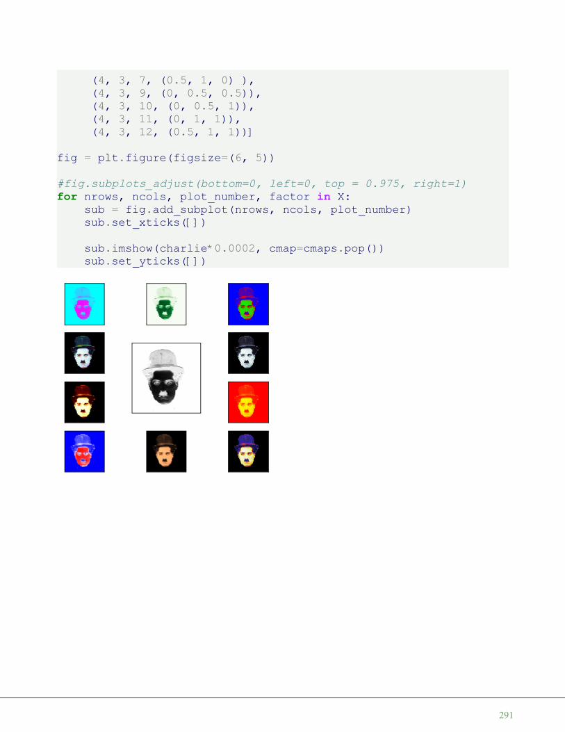
(4, 3, 7, (0.5, 1, 0) ),(4, 3, 9, (0, 0.5, 0.5)),(4, 3, 10, (0, 0.5, 1)),(4, 3, 11, (0, 1, 1)),(4, 3, 12, (0.5, 1, 1))]

fig = plt.figure(figsize=(6, 5))

#fig.subplots_adjust(bottom=0, left=0, top = 0.975, right=1)for nrows, ncols, plot_number, factor in X:

sub = fig.add_subplot(nrows, ncols, plot_number)sub.set_xticks([])

sub.imshow(charlie*0.0002, cmap=cmaps.pop())sub.set_yticks([])

291

I M A G E P R O C E S S I N G T E C H N I Q U E S

INTRODUCTION

As you may have noticed, each of our pages in our varioustutorials are introduced by eye candy pictures, which havecreated with great care to enrich the content. One of thoseimages has been the raison d'être of this chapter. We want todemonstrate how we created the picture for our chapter onDecorators. The idea was to play with decorators in "reallife", small icons with images of small workers painting aroom and on the other hand blending this with the "at" sign,the Python symbol for decorator. It is also a good exampleof how to create a watermark.

We will demonstrate in this chapter the whole process chainof how we created this image. The picture on the right sideof the current page has also been created the same way butuses a director's chair on a small painters background as awatermark instead of the at sign.

At first, we write a function "imag_tile" for tiling imagesboth in horizontal and in vertical direction. We will use thisto create the background of our image.

Then we show how to cut out with slicing a cutout or anexcerpt of an image. We will use the shade function, whichwe introduced in our previous chapter on image processing, to shade our image.

Finally, we will use the original image, the shaded image, plus an image with a binary at sign with theconditional numpy where function to create the final image. The final image contains the at sign as awatermark, cut out from the shaded image.

TILING AN IMAGE

The function imag_tile, which we are going to design, can be best explained with the following diagram:

292

The function imag_tile

imag_tile(img, n, m)

creates a tiled image by appending an image "img" m times in horizontal direction. After this we append thestrip image consisting of m img images n times in vertical direction.

In the following code, we use a picture of painting decorators as the tile image:

%matplotlib inline

import matplotlib.pyplot as plt

293

import matplotlib.image as mpimgimport numpy as npdef imag_tile(img, n, m=1):

"""The image "img" will be repeated n times invertical and m times in horizontal direction."""

if n == 1:tiled_img = img

else:lst_imgs = []for i in range(n):

lst_imgs.append(img)tiled_img = np.concatenate(lst_imgs, axis=1 )

if m > 1:lst_imgs = []for i in range(m):

lst_imgs.append(tiled_img)tiled_img = np.concatenate(lst_imgs, axis=0 )

return tiled_img

basic_pattern = mpimg.imread('decorators_b2.png')

decorators_img = imag_tile(basic_pattern, 3, 3)

plt.axis("off")plt.imshow(decorators_img)

294

An image is a 3-dimensional numpy ndarray.

type(basic_pattern)

The first three rows of our image basic_pattern look like this:

basic_pattern[:3]

Output: <matplotlib.image.AxesImage at 0x7f0c1a6ff390>

Output: numpy.ndarray

295

The innermost lists of our image contain the pixels. We have three values corresponding the the R, G, and Bvalues, this means that we have a 24-bit RGB PNG image, eight bits for each of R, G, B.

PNG images might also consist of 32-bit images (RGBA). The fourth value "A" will be used for transparancy,single channel grayscale.

It's easy to access indivual pixels by indexing, e.g. the pixel in row 100 and column 20:

basic_pattern[100, 28]

As we have seen, the pixels are float (float32) values between 0 and 1. Matplotlib plotting can handle bothfloat32 and uint8 for PNG images. For all other formats it will be only uint8.

Output: array([[[1., 1., 1.],[1., 1., 1.],[1., 1., 1.],...,[1., 1., 1.],[1., 1., 1.],[1., 1., 1.]],

[[1., 1., 1.],[1., 1., 1.],[1., 1., 1.],...,[1., 1., 1.],[1., 1., 1.],[1., 1., 1.]],

[[1., 1., 1.],[1., 1., 1.],[1., 1., 1.],...,[1., 1., 1.],[1., 1., 1.],[1., 1., 1.]]], dtype=float32)

Output: array([0.9019608, 0.8901961, 0.8627451], dtype=float32)

296

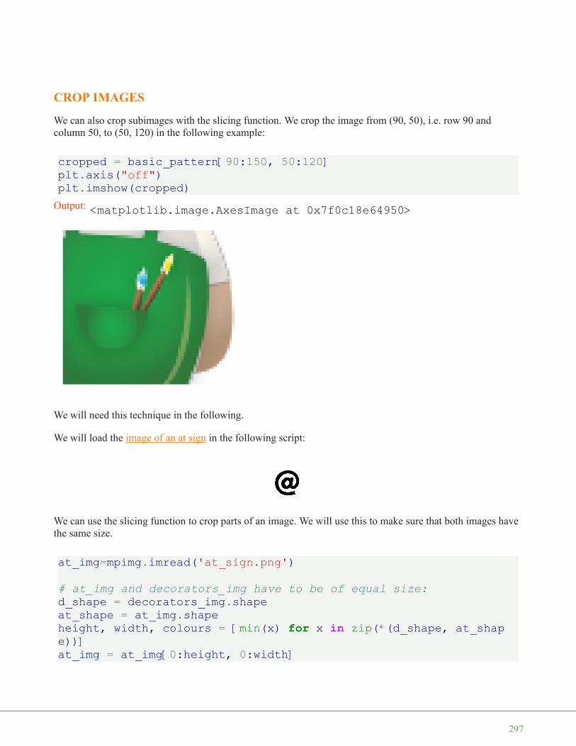
CROP IMAGES

We can also crop subimages with the slicing function. We crop the image from (90, 50), i.e. row 90 andcolumn 50, to (50, 120) in the following example:

cropped = basic_pattern[90:150, 50:120]plt.axis("off")plt.imshow(cropped)

We will need this technique in the following.

We will load the image of an at sign in the following script:

We can use the slicing function to crop parts of an image. We will use this to make sure that both images havethe same size.

at_img=mpimg.imread('at_sign.png')

# at_img and decorators_img have to be of equal size:d_shape = decorators_img.shapeat_shape = at_img.shapeheight, width, colours = [min(x) for x in zip(*(d_shape, at_shape))]at_img = at_img[0:height, 0:width]

Output: <matplotlib.image.AxesImage at 0x7f0c18e64950>

297

SHADE AN IMAGE

We define a function "shade" in the following script. "shade" takes two parameters. The first one "imag" is theimage, which will be shaded and the second one is the shading factor. It can be a value between 0 and 1. If thefactor is set to 0, imag will remain unchanged. If set to one, the image will be completetely blackened.

def shade(imag, percent):"""imag: the image which will be shadedpercent: a value between 0 (image will remain unchanged

and 1 (image will be blackened)"""tinted_imag = imag * (1 - percent)return tinted_imag

tinted_decorator_img = shade(decorators_img, 0.5)plt.imshow(tinted_decorator_img)print(tinted_decorator_img[:3])

298

[[[0.5 0.5 0.5][0.5 0.5 0.5][0.5 0.5 0.5]...[0.5 0.5 0.5][0.5 0.5 0.5][0.5 0.5 0.5]]

[[0.5 0.5 0.5][0.5 0.5 0.5][0.5 0.5 0.5]...[0.5 0.5 0.5][0.5 0.5 0.5][0.5 0.5 0.5]]

[[0.5 0.5 0.5][0.5 0.5 0.5][0.5 0.5 0.5]...[0.5 0.5 0.5][0.5 0.5 0.5][0.5 0.5 0.5]]]

299

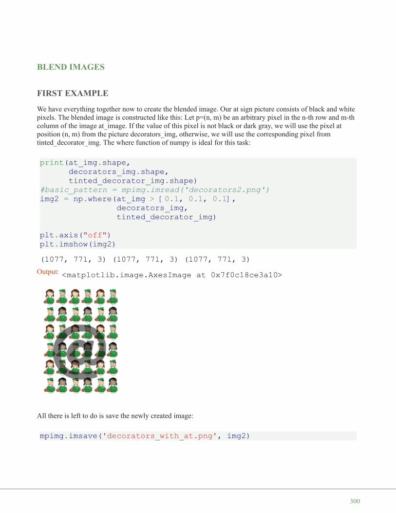
BLEND IMAGES

FIRST EXAMPLE

We have everything together now to create the blended image. Our at sign picture consists of black and whitepixels. The blended image is constructed like this: Let p=(n, m) be an arbitrary pixel in the n-th row and m-thcolumn of the image at_image. If the value of this pixel is not black or dark gray, we will use the pixel atposition (n, m) from the picture decorators_img, otherwise, we will use the corresponding pixel fromtinted_decorator_img. The where function of numpy is ideal for this task:

print(at_img.shape,decorators_img.shape,tinted_decorator_img.shape)

#basic_pattern = mpimg.imread('decorators2.png')img2 = np.where(at_img > [0.1, 0.1, 0.1],

decorators_img,tinted_decorator_img)

plt.axis("off")plt.imshow(img2)

All there is left to do is save the newly created image:

mpimg.imsave('decorators_with_at.png', img2)

(1077, 771, 3) (1077, 771, 3) (1077, 771, 3)Output: <matplotlib.image.AxesImage at 0x7f0c18ce3a10>

300

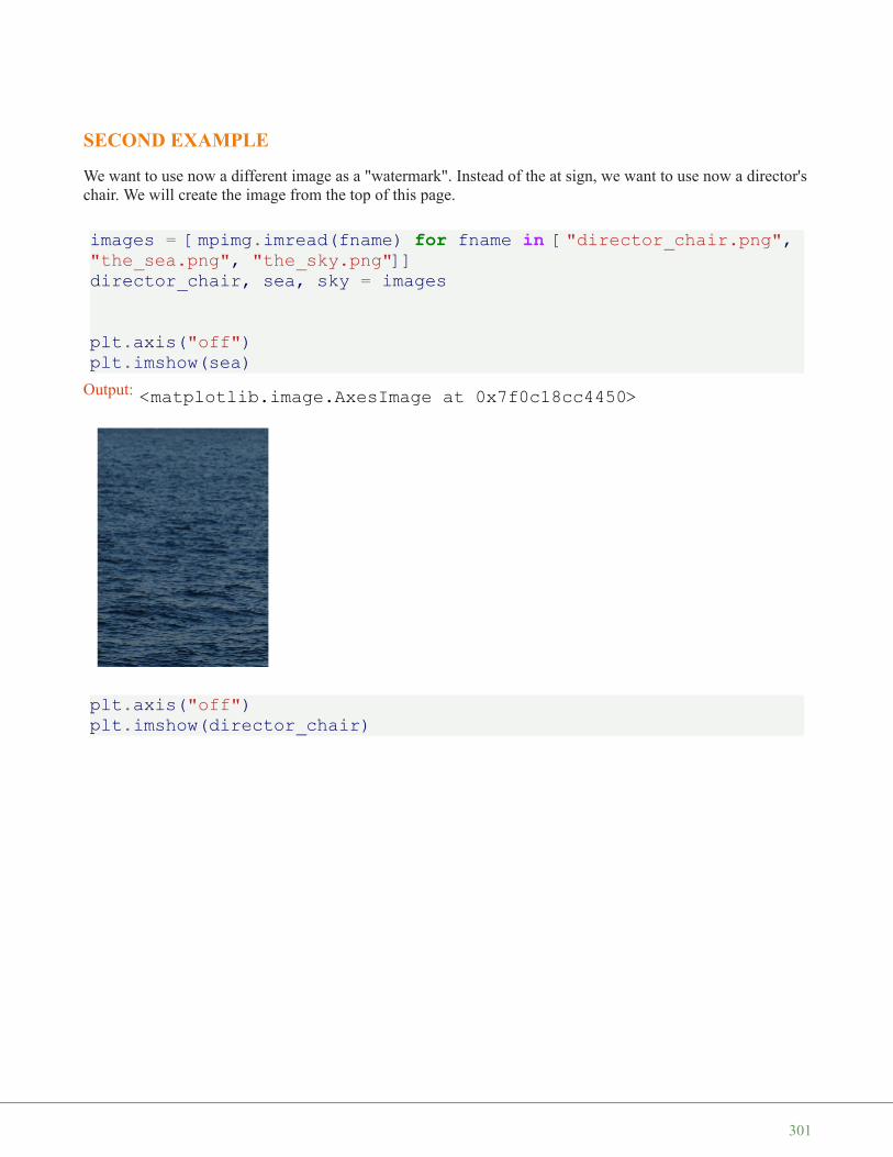
SECOND EXAMPLE

We want to use now a different image as a "watermark". Instead of the at sign, we want to use now a director'schair. We will create the image from the top of this page.

images = [mpimg.imread(fname) for fname in ["director_chair.png","the_sea.png", "the_sky.png"]]director_chair, sea, sky = images

plt.axis("off")plt.imshow(sea)

plt.axis("off")plt.imshow(director_chair)

Output: <matplotlib.image.AxesImage at 0x7f0c18cc4450>

301

In the following, we blend together the images director_chair, decorators_img and sea by using where ofnumpy once more:

#sea2 = mpimg.imread('the_sea2.png')img = np.where(director_chair > [0.9, 0.9, 0.9],

decorators_img,sea)

plt.axis("off")plt.imshow(img)mpimg.imsave('decorators_with_chair.png', img)

We could have used "Image.open" from PIL instead of mpimg.imread from matplotlib to read in the pictures.There is a crucial difference or a potential "problem" between these two ways: The image we get from imreadhas values between 0 and 1, whereas Image.open consists of values between 0 and 255. So we might have todivide all the pixels by 255, if we have to work with an image read in by mpimg.imread:

Output: <matplotlib.image.AxesImage at 0x7f0c18423850>

302

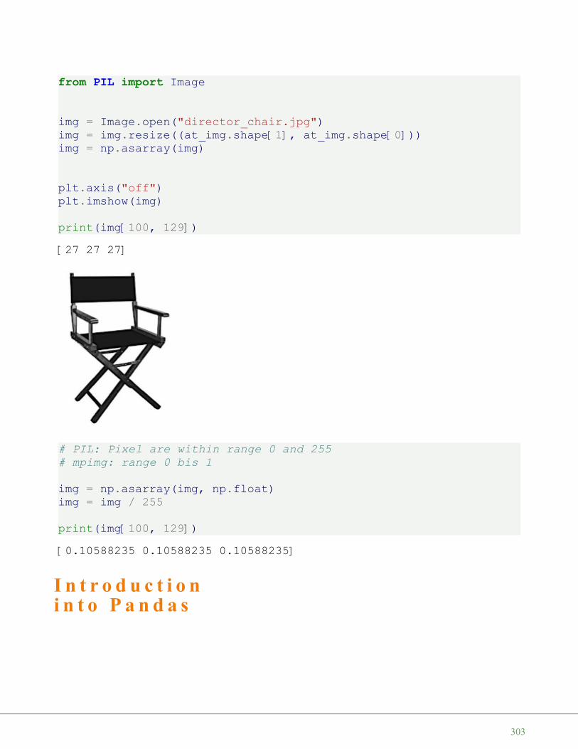
from PIL import Image

img = Image.open("director_chair.jpg")img = img.resize((at_img.shape[1], at_img.shape[0]))img = np.asarray(img)

plt.axis("off")plt.imshow(img)

print(img[100, 129])

# PIL: Pixel are within range 0 and 255# mpimg: range 0 bis 1

img = np.asarray(img, np.float)img = img / 255

print(img[100, 129])

I n t r o d u c t i o ni n t o P a n d a s

[27 27 27]

[0.10588235 0.10588235 0.10588235]

303

The pandas we are writing about in this chapter havenothing to do with the cute panda bears. Endearing bearsare not what our visitors expect in a Python tutorial.Pandas is the name for a Python module, which isrounding up the capabilities of Numpy, Scipy andMatplotlab. The word pandas is an acronym which isderived from "Python and data analysis" and "panel data".

There is often some confusion about whether Pandas is analternative to Numpy, SciPy and Matplotlib. The truth isthat it is built on top of Numpy. This means that Numpy isrequired by pandas. Scipy and Matplotlib on the otherhand are not required by pandas but they are extremelyuseful. That's why the Pandas project lists them as"optional dependency".

Pandas is a software library written for the Python programming language. It is used for data manipulation andanalysis. It provides special data structures and operations for the manipulation of numerical tables and timeseries. Pandas is free software released under the three-clause BSD license.

304

D A T A S T R U C T U R E S

We will start with the following two important data structures of Pandas:

• Series and• DataFrame

SERIES

A Series is a one-dimensional labelled array-like object. It is capable of holding any data type, e.g. integers,floats, strings, Python objects, and so on. It can be seen as a data structure with two arrays: one functioning asthe index, i.e. the labels, and the other one contains the actual data.

We define a simple Series object in the following example by instantiating a Pandas Series object with a list.We will later see that we can use other data objects for example Numpy arrays and dictionaries as well toinstantiate a Series object.

import pandas as pdS = pd.Series([11, 28, 72, 3, 5, 8])S

We haven't defined an index in our example, but we see two columns in our output: The right column containsour data, whereas the left column contains the index. Pandas created a default index starting with 0 going to 5,which is the length of the data minus 1.

We can directly access the index and the values of our Series S:

print(S.index)print(S.values)

If we compare this to creating an array in numpy, we will find lots of similarities:

Output: 0 111 282 723 34 55 8dtype: int64

RangeIndex(start=0, stop=6, step=1)[11 28 72 3 5 8]

305

import numpy as npX = np.array([11, 28, 72, 3, 5, 8])print(X)print(S.values)# both are the same type:print(type(S.values), type(X))

So far our Series have not been very different to ndarrays of Numpy. This changes, as soon as we startdefining Series objects with individual indices:

fruits = ['apples', 'oranges', 'cherries', 'pears']quantities = [20, 33, 52, 10]S = pd.Series(quantities, index=fruits)S

A big advantage to NumPy arrays is obvious from the previous example: We can use arbitrary indices.

If we add two series with the same indices, we get a new series with the same index and the correpondingvalues will be added:

fruits = ['apples', 'oranges', 'cherries', 'pears']

S = pd.Series([20, 33, 52, 10], index=fruits)S2 = pd.Series([17, 13, 31, 32], index=fruits)print(S + S2)print("sum of S: ", sum(S))

The indices do not have to be the same for the Series addition. The index will be the "union" of both indices. If

[11 28 72 3 5 8][11 28 72 3 5 8]<class 'numpy.ndarray'> <class 'numpy.ndarray'>

Output: apples 20oranges 33cherries 52pears 10dtype: int64

apples 37oranges 46cherries 83pears 42dtype: int64sum of S: 115

306

an index doesn't occur in both Series, the value for this Series will be NaN:

fruits = ['peaches', 'oranges', 'cherries', 'pears']fruits2 = ['raspberries', 'oranges', 'cherries', 'pears']

S = pd.Series([20, 33, 52, 10], index=fruits)S2 = pd.Series([17, 13, 31, 32], index=fruits2)print(S + S2)

In principle, the indices can be completely different, as in the following example. We have two indices. One isthe Turkish translation of the English fruit names:

fruits = ['apples', 'oranges', 'cherries', 'pears']

fruits_tr = ['elma', 'portakal', 'kiraz', 'armut']

S = pd.Series([20, 33, 52, 10], index=fruits)S2 = pd.Series([17, 13, 31, 32], index=fruits_tr)print(S + S2)

INDEXING

It's possible to access single values of a Series.

print(S['apples'])

cherries 83.0oranges 46.0peaches NaNpears 42.0raspberries NaNdtype: float64

apples NaNarmut NaNcherries NaNelma NaNkiraz NaNoranges NaNpears NaNportakal NaNdtype: float64

20

307

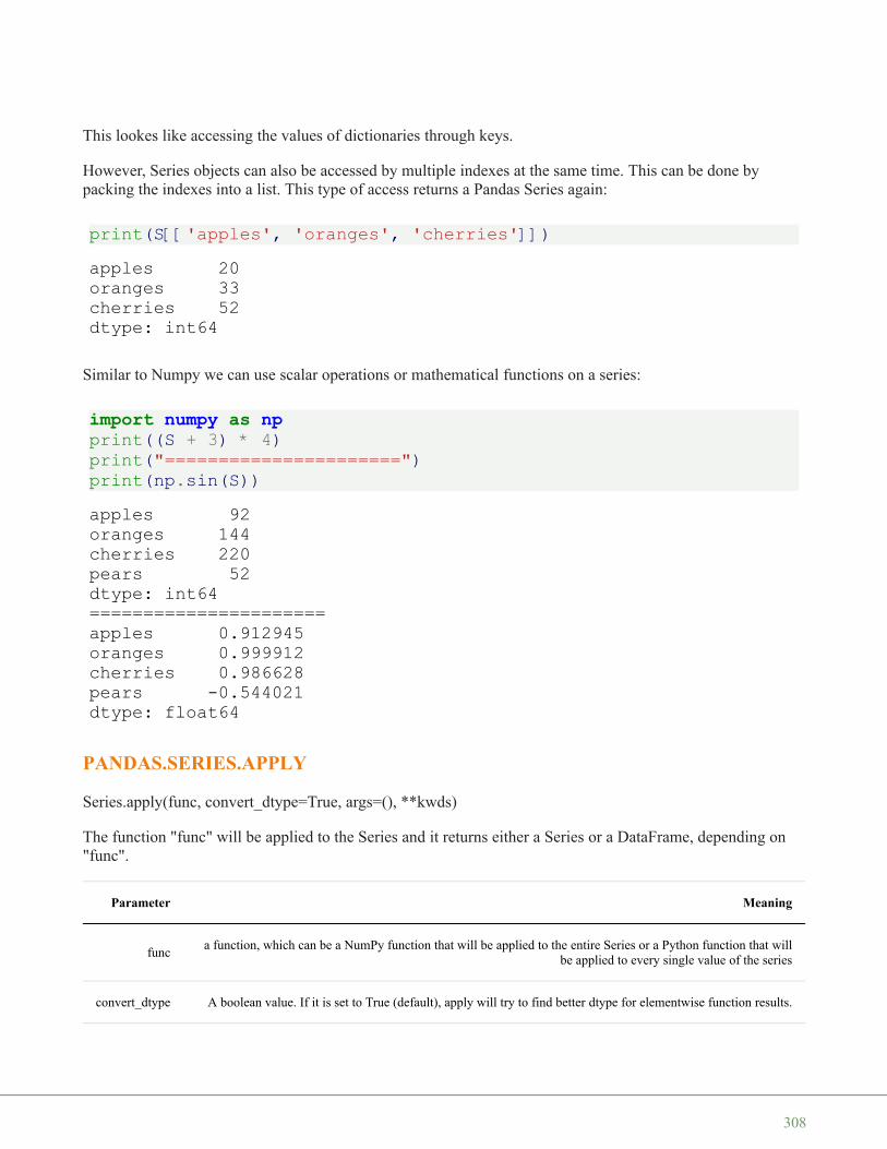
This lookes like accessing the values of dictionaries through keys.

However, Series objects can also be accessed by multiple indexes at the same time. This can be done bypacking the indexes into a list. This type of access returns a Pandas Series again:

print(S[['apples', 'oranges', 'cherries']])

Similar to Numpy we can use scalar operations or mathematical functions on a series:

import numpy as npprint((S + 3) * 4)print("======================")print(np.sin(S))

PANDAS.SERIES.APPLY

Series.apply(func, convert_dtype=True, args=(), **kwds)

The function "func" will be applied to the Series and it returns either a Series or a DataFrame, depending on"func".

Parameter Meaning

funca function, which can be a NumPy function that will be applied to the entire Series or a Python function that will

be applied to every single value of the series

convert_dtype A boolean value. If it is set to True (default), apply will try to find better dtype for elementwise function results.

apples 20oranges 33cherries 52dtype: int64

apples 92oranges 144cherries 220pears 52dtype: int64======================apples 0.912945oranges 0.999912cherries 0.986628pears -0.544021dtype: float64

308

Parameter Meaning

If False, leave as dtype=object

args Positional arguments which will be passed to the function "func" additionally to the values from the series.

**kwds Additional keyword arguments will be passed as keywords to the function

Example:

S.apply(np.log)

We can also use Python lambda functions. Let's assume, we have the following task. The test the amount offruit for every kind. If there are less than 50 available, we will augment the stock by 10:

S.apply(lambda x: x if x > 50 else x+10 )

FILTERING WITH A BOOLEAN ARRAY

Similar to numpy arrays, we can filter Pandas Series with a Boolean array:

S[S>30]

A series can be seen as an ordered Python dictionary with a fixed length.

"apples" in S

Output: apples 2.995732oranges 3.496508cherries 3.951244pears 2.302585dtype: float64

Output: apples 30oranges 43cherries 52pears 20dtype: int64

Output: oranges 33cherries 52dtype: int64

309

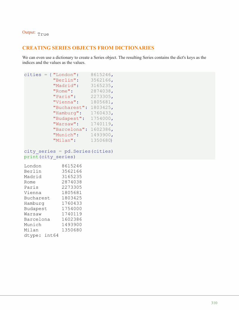
CREATING SERIES OBJECTS FROM DICTIONARIES

We can even use a dictionary to create a Series object. The resulting Series contains the dict's keys as theindices and the values as the values.

cities = {"London": 8615246,"Berlin": 3562166,"Madrid": 3165235,"Rome": 2874038,"Paris": 2273305,"Vienna": 1805681,"Bucharest": 1803425,"Hamburg": 1760433,"Budapest": 1754000,"Warsaw": 1740119,"Barcelona": 1602386,"Munich": 1493900,"Milan": 1350680}

city_series = pd.Series(cities)print(city_series)

Output: True

London 8615246Berlin 3562166Madrid 3165235Rome 2874038Paris 2273305Vienna 1805681Bucharest 1803425Hamburg 1760433Budapest 1754000Warsaw 1740119Barcelona 1602386Munich 1493900Milan 1350680dtype: int64

310

NAN - MISSING DATA

One problem in dealing with data analysistasks consists in missing data. Pandasmakes it as easy as possible to work withmissing data.

If we look once more at our previousexample, we can see that the index of ourseries is the same as the keys of thedictionary we used to create thecities_series. Now, we want to use anindex which is not overlapping with thedictionary keys. We have already seenthat we can pass a list or a tuple to thekeyword argument 'index' to define theindex. In our next example, the list (ortuple) passed to the keyword parameter'index' will not be equal to the keys. Thismeans that some cities from thedictionary will be missing and two cities("Zurich" and "Stuttgart") don't occur in the dictionary.

my_cities = ["London", "Paris", "Zurich", "Berlin","Stuttgart", "Hamburg"]

my_city_series = pd.Series(cities,index=my_cities)

my_city_series

Due to the Nan values the population values for the other cities are turned into floats. There is no missing datain the following examples, so the values are int:

my_cities = ["London", "Paris", "Berlin", "Hamburg"]

my_city_series = pd.Series(cities,index=my_cities)

my_city_series

Output: London 8615246.0Paris 2273305.0Zurich NaNBerlin 3562166.0Stuttgart NaNHamburg 1760433.0dtype: float64

311

THE METHODS ISNULL() AND NOTNULL()

We can see, that the cities, which are not included in the dictionary, get the value NaN assigned. NaN standsfor "not a number". It can also be seen as meaning "missing" in our example.

We can check for missing values with the methods isnull and notnull:

my_cities = ["London", "Paris", "Zurich", "Berlin","Stuttgart", "Hamburg"]

my_city_series = pd.Series(cities,index=my_cities)

print(my_city_series.isnull())

print(my_city_series.notnull())

CONNECTION BETWEEN NAN AND NONE

We get also a NaN, if a value in the dictionary has a None:

d = {"a":23, "b":45, "c":None, "d":0}S = pd.Series(d)print(S)

Output: London 8615246Paris 2273305Berlin 3562166Hamburg 1760433dtype: int64

London FalseParis FalseZurich TrueBerlin FalseStuttgart TrueHamburg Falsedtype: bool

London TrueParis TrueZurich FalseBerlin TrueStuttgart FalseHamburg Truedtype: bool

312

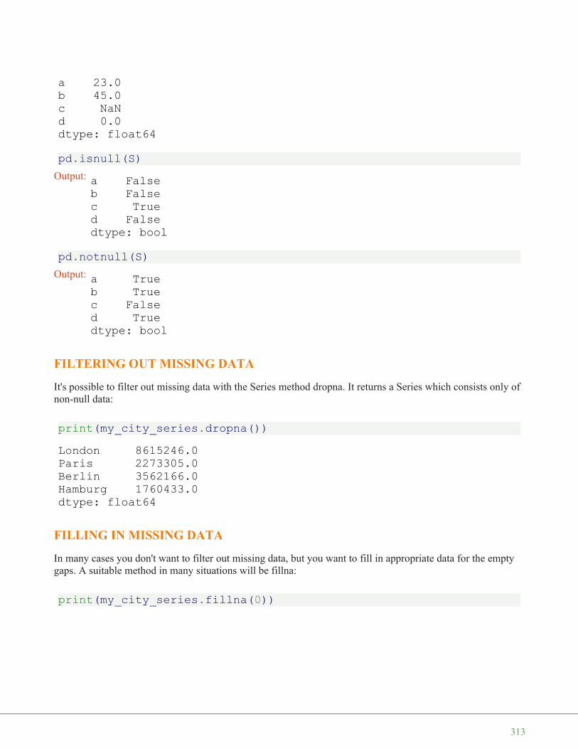
pd.isnull(S)

pd.notnull(S)

FILTERING OUT MISSING DATA

It's possible to filter out missing data with the Series method dropna. It returns a Series which consists only ofnon-null data:

print(my_city_series.dropna())

FILLING IN MISSING DATA

In many cases you don't want to filter out missing data, but you want to fill in appropriate data for the emptygaps. A suitable method in many situations will be fillna:

print(my_city_series.fillna(0))

a 23.0b 45.0c NaNd 0.0dtype: float64

Output: a Falseb Falsec Trued Falsedtype: bool

Output: a Trueb Truec Falsed Truedtype: bool

London 8615246.0Paris 2273305.0Berlin 3562166.0Hamburg 1760433.0dtype: float64

313

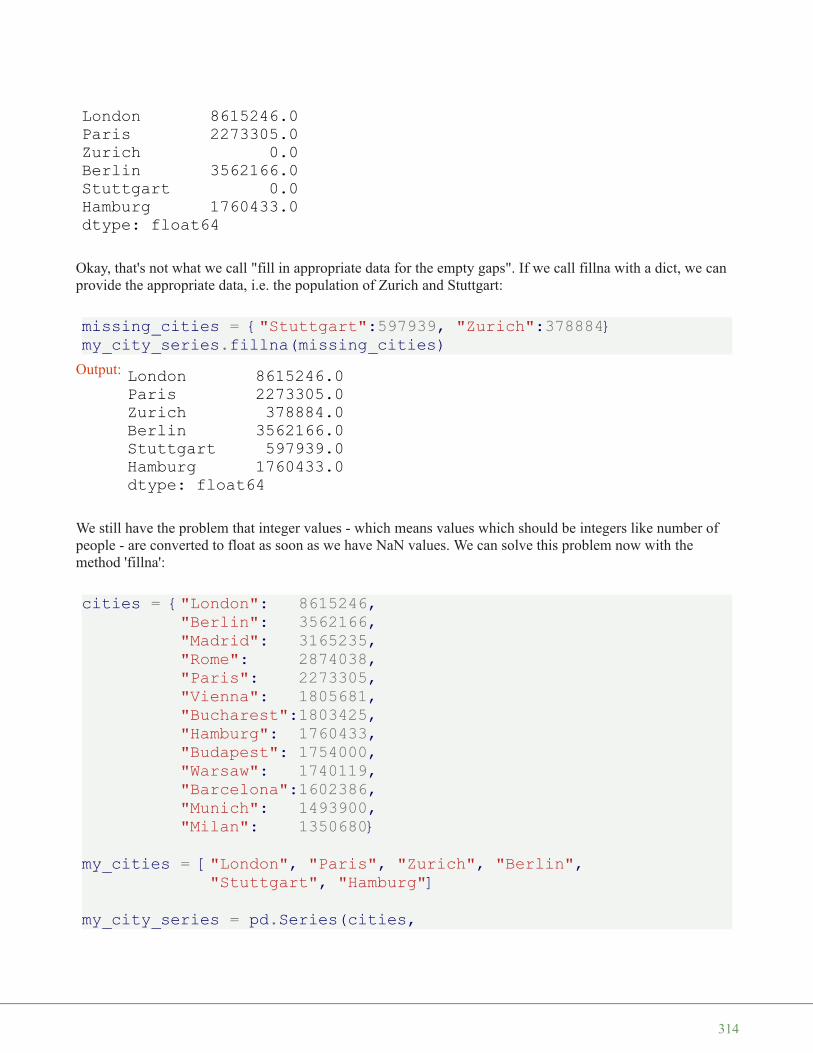
Okay, that's not what we call "fill in appropriate data for the empty gaps". If we call fillna with a dict, we canprovide the appropriate data, i.e. the population of Zurich and Stuttgart:

missing_cities = {"Stuttgart":597939, "Zurich":378884}my_city_series.fillna(missing_cities)

We still have the problem that integer values - which means values which should be integers like number ofpeople - are converted to float as soon as we have NaN values. We can solve this problem now with themethod 'fillna':

cities = {"London": 8615246,"Berlin": 3562166,"Madrid": 3165235,"Rome": 2874038,"Paris": 2273305,"Vienna": 1805681,"Bucharest":1803425,"Hamburg": 1760433,"Budapest": 1754000,"Warsaw": 1740119,"Barcelona":1602386,"Munich": 1493900,"Milan": 1350680}

my_cities = ["London", "Paris", "Zurich", "Berlin","Stuttgart", "Hamburg"]

my_city_series = pd.Series(cities,

London 8615246.0Paris 2273305.0Zurich 0.0Berlin 3562166.0Stuttgart 0.0Hamburg 1760433.0dtype: float64

Output: London 8615246.0Paris 2273305.0Zurich 378884.0Berlin 3562166.0Stuttgart 597939.0Hamburg 1760433.0dtype: float64

314

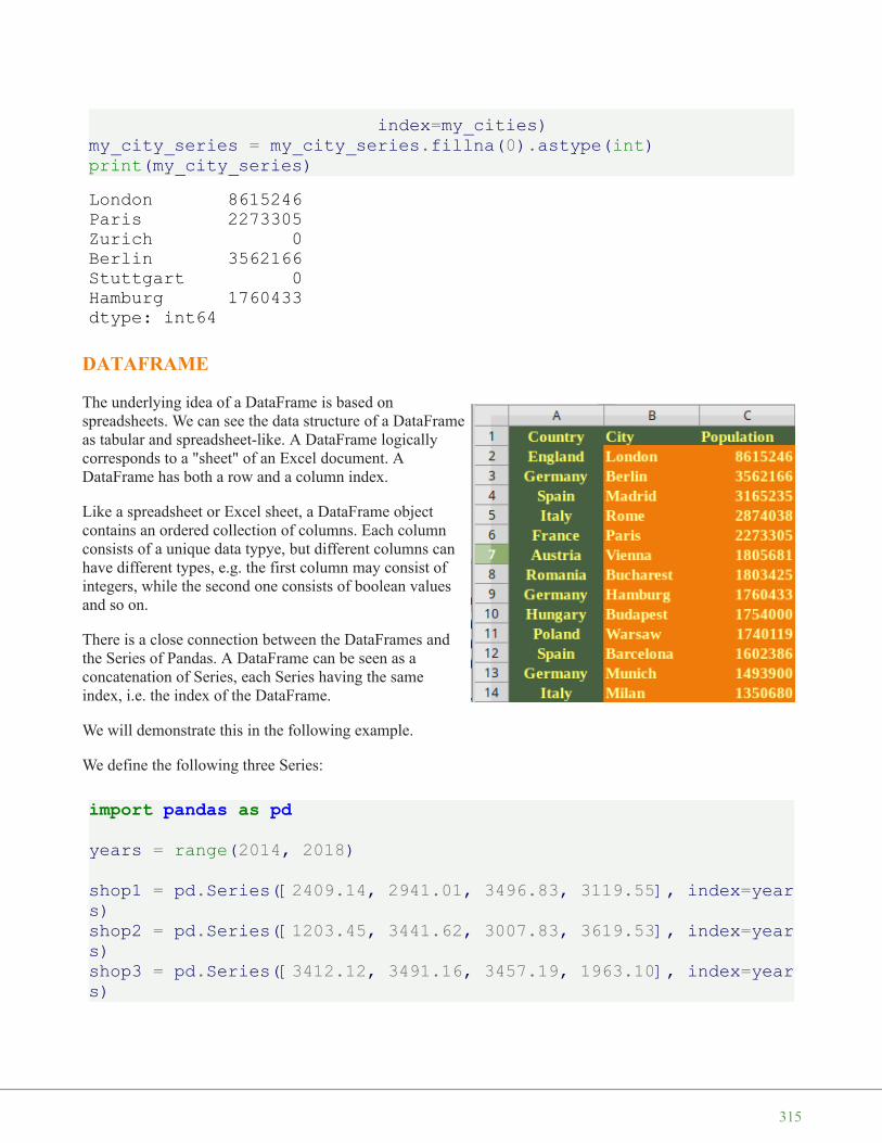
index=my_cities)my_city_series = my_city_series.fillna(0).astype(int)print(my_city_series)

DATAFRAME

The underlying idea of a DataFrame is based onspreadsheets. We can see the data structure of a DataFrameas tabular and spreadsheet-like. A DataFrame logicallycorresponds to a "sheet" of an Excel document. ADataFrame has both a row and a column index.

Like a spreadsheet or Excel sheet, a DataFrame objectcontains an ordered collection of columns. Each columnconsists of a unique data typye, but different columns canhave different types, e.g. the first column may consist ofintegers, while the second one consists of boolean valuesand so on.

There is a close connection between the DataFrames andthe Series of Pandas. A DataFrame can be seen as aconcatenation of Series, each Series having the sameindex, i.e. the index of the DataFrame.

We will demonstrate this in the following example.

We define the following three Series:

import pandas as pdyears = range(2014, 2018)

shop1 = pd.Series([2409.14, 2941.01, 3496.83, 3119.55], index=years)shop2 = pd.Series([1203.45, 3441.62, 3007.83, 3619.53], index=years)shop3 = pd.Series([3412.12, 3491.16, 3457.19, 1963.10], index=years)

London 8615246Paris 2273305Zurich 0Berlin 3562166Stuttgart 0Hamburg 1760433dtype: int64

315

What happens, if we concatenate these "shop" Series? Pandas provides a concat function for this purpose:

pd.concat([shop1, shop2, shop3])

This result is not what we have intended or expected. The reason is that concat used 0 as the default for theaxis parameter. Let's do it with "axis=1":

shops_df = pd.concat([shop1, shop2, shop3], axis=1)shops_df

Let's do some fine sanding by giving names to the columns:

cities = ["Zürich", "Winterthur", "Freiburg"]shops_df.columns = citiesprint(shops_df)

# alternative way: give names to series:shop1.name = "Zürich"

Output: 2014 2409.142015 2941.012016 3496.832017 3119.552014 1203.452015 3441.622016 3007.832017 3619.532014 3412.122015 3491.162016 3457.192017 1963.10dtype: float64

Output:

0 1 2

2014 2409.14 1203.45 3412.12

2015 2941.01 3441.62 3491.16

2016 3496.83 3007.83 3457.19

2017 3119.55 3619.53 1963.10

316

shop2.name = "Winterthur"shop3.name = "Freiburg"

print("------")shops_df2 = pd.concat([shop1, shop2, shop3], axis=1)print(shops_df2)

This was nice, but what kind of data type is our result?

print(type(shops_df))

This means, we can arrange or concat Series into DataFrames!

DATAFRAMES FROM DICTIONARIES

A DataFrame has a row and column index; it's like a dict of Series with a common index.

cities = {"name": ["London", "Berlin", "Madrid", "Rome","Paris", "Vienna", "Bucharest", "Hamburg","Budapest", "Warsaw", "Barcelona","Munich", "Milan"],

"population": [8615246, 3562166, 3165235, 2874038,2273305, 1805681, 1803425, 1760433,1754000, 1740119, 1602386, 1493900,1350680],

"country": ["England", "Germany", "Spain", "Italy","France", "Austria", "Romania","Germany", "Hungary", "Poland", "Spain","Germany", "Italy"]}

Zürich Winterthur Freiburg2014 2409.14 1203.45 3412.122015 2941.01 3441.62 3491.162016 3496.83 3007.83 3457.192017 3119.55 3619.53 1963.10------

Zürich Winterthur Freiburg2014 2409.14 1203.45 3412.122015 2941.01 3441.62 3491.162016 3496.83 3007.83 3457.192017 3119.55 3619.53 1963.10

<class 'pandas.core.frame.DataFrame'>

317

city_frame = pd.DataFrame(cities)city_frame

RETRIEVING THE COLUMN NAMES

It's possible to get the names of the columns as a list:

city_frame.columns.values

CUSTOM INDEX

We can see that an index (0,1,2, ...) has been automatically assigned to the DataFrame. We can also assign a

Output:

name population country

0 London 8615246 England

1 Berlin 3562166 Germany

2 Madrid 3165235 Spain

3 Rome 2874038 Italy

4 Paris 2273305 France

5 Vienna 1805681 Austria

6 Bucharest 1803425 Romania

7 Hamburg 1760433 Germany

8 Budapest 1754000 Hungary

9 Warsaw 1740119 Poland

10 Barcelona 1602386 Spain

11 Munich 1493900 Germany

12 Milan 1350680 Italy

Output: array(['name', 'population', 'country'], dtype=object)

318

custom index to the DataFrame object:

ordinals = ["first", "second", "third", "fourth","fifth", "sixth", "seventh", "eigth","ninth", "tenth", "eleventh", "twelvth","thirteenth"]

city_frame = pd.DataFrame(cities, index=ordinals)city_frame

REARRANGING THE ORDER OF COLUMNS

We can also define and rearrange the order of the columns at the time of creation of the DataFrame. Thismakes also sure that we will have a defined ordering of our columns, if we create the DataFrame from a

Output:

name population country

first London 8615246 England

second Berlin 3562166 Germany

third Madrid 3165235 Spain

fourth Rome 2874038 Italy

fifth Paris 2273305 France

sixth Vienna 1805681 Austria

seventh Bucharest 1803425 Romania

eigth Hamburg 1760433 Germany

ninth Budapest 1754000 Hungary

tenth Warsaw 1740119 Poland

eleventh Barcelona 1602386 Spain

twelvth Munich 1493900 Germany

thirteenth Milan 1350680 Italy

319

dictionary. Dictionaries are not ordered, as you have seen in our chapter on Dictionaries in our Python tutorial,so we cannot know in advance what the ordering of our columns will be:

city_frame = pd.DataFrame(cities,columns=["name",

"country","population"])

city_frame

We change both the column order and the ordering of the index with the function reindex with thefollowing code:

city_frame.reindex(index=[0, 2, 4, 6, 8, 10, 12, 1, 3, 5, 7, 9, 1

Output:

name country population

0 London England 8615246

1 Berlin Germany 3562166

2 Madrid Spain 3165235

3 Rome Italy 2874038

4 Paris France 2273305

5 Vienna Austria 1805681

6 Bucharest Romania 1803425

7 Hamburg Germany 1760433

8 Budapest Hungary 1754000

9 Warsaw Poland 1740119

10 Barcelona Spain 1602386

11 Munich Germany 1493900

12 Milan Italy 1350680

320

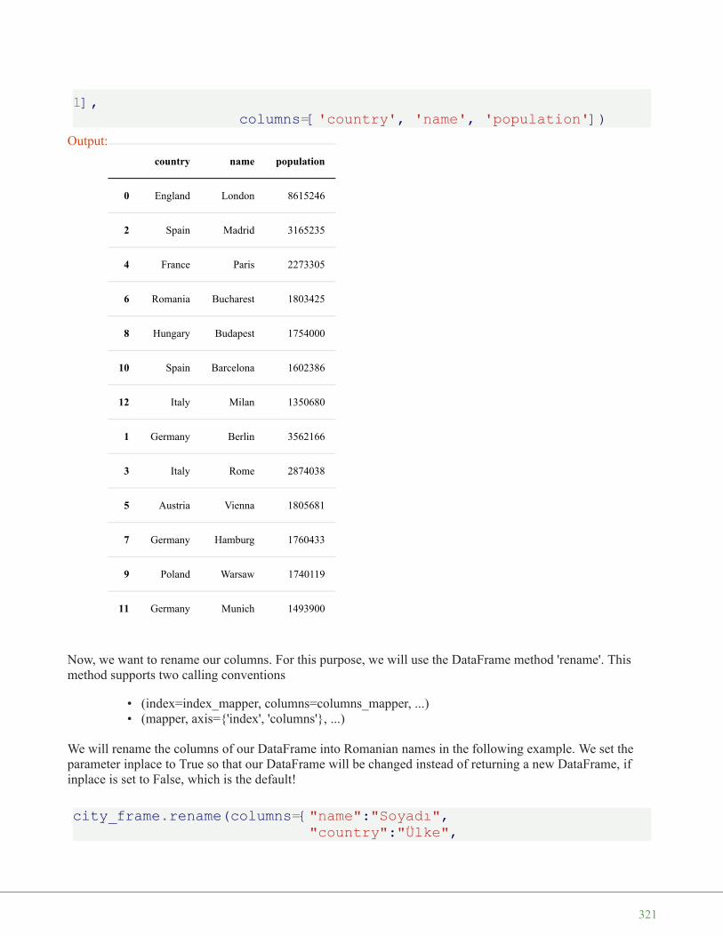
1],columns=['country', 'name', 'population'])

Now, we want to rename our columns. For this purpose, we will use the DataFrame method 'rename'. Thismethod supports two calling conventions

• (index=index_mapper, columns=columns_mapper, ...)• (mapper, axis={'index', 'columns'}, ...)

We will rename the columns of our DataFrame into Romanian names in the following example. We set theparameter inplace to True so that our DataFrame will be changed instead of returning a new DataFrame, ifinplace is set to False, which is the default!

city_frame.rename(columns={"name":"Soyadı","country":"Ülke",

Output:

country name population

0 England London 8615246

2 Spain Madrid 3165235

4 France Paris 2273305

6 Romania Bucharest 1803425

8 Hungary Budapest 1754000

10 Spain Barcelona 1602386

12 Italy Milan 1350680

1 Germany Berlin 3562166

3 Italy Rome 2874038

5 Austria Vienna 1805681

7 Germany Hamburg 1760433

9 Poland Warsaw 1740119

11 Germany Munich 1493900

321

"population":"Nüfus"},inplace=True)

city_frame

EXISTING COLUMN AS THE INDEX OF A DATAFRAME

We want to create a more useful index in the following example. We will use the country name as the index,i.e. the list value associated to the key "country" of our cities dictionary:

city_frame = pd.DataFrame(cities,columns=["name", "population"],index=cities["country"])

city_frame

Output:

Soyadı Ülke Nüfus

0 London England 8615246

1 Berlin Germany 3562166

2 Madrid Spain 3165235

3 Rome Italy 2874038

4 Paris France 2273305

5 Vienna Austria 1805681

6 Bucharest Romania 1803425

7 Hamburg Germany 1760433

8 Budapest Hungary 1754000

9 Warsaw Poland 1740119

10 Barcelona Spain 1602386

11 Munich Germany 1493900

12 Milan Italy 1350680

322

Alternatively, we can change an existing DataFrame. We can us the method set_index to turn a column into anindex. "set_index" does not work in-place, it returns a new data frame with the chosen column as the index:

city_frame = pd.DataFrame(cities)city_frame2 = city_frame.set_index("country")print(city_frame2)

Output:

name population

England London 8615246

Germany Berlin 3562166

Spain Madrid 3165235

Italy Rome 2874038

France Paris 2273305

Austria Vienna 1805681

Romania Bucharest 1803425

Germany Hamburg 1760433

Hungary Budapest 1754000

Poland Warsaw 1740119

Spain Barcelona 1602386

Germany Munich 1493900

Italy Milan 1350680

323

We saw in the previous example that the set_index method returns a new DataFrame object and doesn't changethe original DataFrame. If we set the optional parameter "inplace" to True, the DataFrame will be changed inplace, i.e. no new object will be created:

city_frame = pd.DataFrame(cities)city_frame.set_index("country", inplace=True)print(city_frame)

ACCESSING ROWS VIA INDEX VALUES

So far we have accessed DataFrames via the columns. It is often necessary to select certain rows via the indexnames. We will demonstrate now, how we can access rows from DataFrames via the locators 'loc' and 'iloc'.We will not cover 'ix' because it is deprecated and will be removed in the future.

name populationcountryEngland London 8615246Germany Berlin 3562166Spain Madrid 3165235Italy Rome 2874038France Paris 2273305Austria Vienna 1805681Romania Bucharest 1803425Germany Hamburg 1760433Hungary Budapest 1754000Poland Warsaw 1740119Spain Barcelona 1602386Germany Munich 1493900Italy Milan 1350680

name populationcountryEngland London 8615246Germany Berlin 3562166Spain Madrid 3165235Italy Rome 2874038France Paris 2273305Austria Vienna 1805681Romania Bucharest 1803425Germany Hamburg 1760433Hungary Budapest 1754000Poland Warsaw 1740119Spain Barcelona 1602386Germany Munich 1493900Italy Milan 1350680

324

We select all the German cities in the following example by using 'loc'. The result is a DataFrame:

city_frame = pd.DataFrame(cities,columns=("name", "population"),index=cities["country"])

print(city_frame.loc["Germany"])

It is also possible to simultaneously extracting rows by chosen more than on index labels. To do this we use alist of indices:

print(city_frame.loc[["Germany", "France"]])

We will also need to select pandas DataFrame rows based on conditions, which are applied to column values.We can use the operators '>', '=', '=', '<=', '!=' for this purpose. We select all cities with a population of morethan two million in the following example:

condition = city_frame.population>2000000condition

name populationGermany Berlin 3562166Germany Hamburg 1760433Germany Munich 1493900

name populationGermany Berlin 3562166Germany Hamburg 1760433Germany Munich 1493900France Paris 2273305

Output: England TrueGermany TrueSpain TrueItaly TrueFrance TrueAustria FalseRomania FalseGermany FalseHungary FalsePoland FalseSpain FalseGermany FalseItaly FalseName: population, dtype: bool

325

We can use this Boolean DataFrame condition with loc to finally create the selection:

print(city_frame.loc[condition])

It is also possible to logically combine more than one condition with & and | :

condition1 = (city_frame.population>1500000)condition2 = (city_frame['name'].str.contains("m"))print(city_frame.loc[condition1 & condition2])

We use a logical or | in the following example to see all cities of the Pandas DataFrame, where either thecity name contains the letter 'm' or the population number is greater than three million:

condition1 = (city_frame.population>3000000)condition2 = (city_frame['name'].str.contains("m"))print(city_frame.loc[condition1 | condition2])

ADDING ROWS TO A DATAFRAMEmilan = ['Milan', 1399860]city_frame.iloc[-1] = milancity_frame.loc['Switzerland'] = ['Zurich', 415215]city_frame

name populationEngland London 8615246Germany Berlin 3562166Spain Madrid 3165235Italy Rome 2874038France Paris 2273305

name populationItaly Rome 2874038Germany Hamburg 1760433

name populationEngland London 8615246Germany Berlin 3562166Spain Madrid 3165235Italy Rome 2874038Germany Hamburg 1760433

326

ACCESSING ROWS BY POSITION

The iloc method of a Pandas DataFrame object can be used to select rows and columns by number, i.e. inthe order that they appear in the data frame. iloc allows selections of the rows, as if they were numberedby integers 0 , 1 , 2 , ....

We demonstrate this in the following example:

df = city_frame.iloc[3]print(df)

Output:

name population

England London 8615246

Germany Berlin 3562166

Spain Madrid 3165235

Italy Rome 2874038

France Paris 2273305

Austria Vienna 1805681

Romania Bucharest 1803425

Germany Hamburg 1760433

Hungary Budapest 1754000

Poland Warsaw 1740119

Spain Barcelona 1602386

Germany Munich 1493900

Italy Milan 1399860

Switzerland Zurich 415215

327

To get a DataFrame with selected rows by numbers, we use a list of integers. We can see that we can changethe order of the rows and we are also able to select rows multiple times:

df = city_frame.iloc[[3, 2, 0, 5, 0]]print(df)

SUM AND CUMULATIVE SUM

The DataFrame object of Pandas provides a method to sum both columns and rows. Before we will explain theusage of the sum method, we will create a new DataFrame object on which we will apply our examples. Wewill start by creating an empty DataFrame without columns but an index. We populate this DataFrame byadding columns with random values:

years = range(2014, 2019)cities = ["Zürich", "Freiburg", "München", "Konstanz", "Saarbrücken"]shops = pd.DataFrame(index=years)for city in cities:

shops.insert(loc=len(shops.columns),column=city,value=(np.random.uniform(0.7, 1, (5,)) * 1000).ro

und(2))

print(shops)

Let's apply sum to the DataFrame shops :

name Romepopulation 2874038Name: Italy, dtype: object

name populationItaly Rome 2874038Spain Madrid 3165235England London 8615246Austria Vienna 1805681England London 8615246

Zürich Freiburg München Konstanz Saarbrücken2014 872.51 838.22 961.17 934.99 796.422015 944.47 943.27 862.66 784.23 770.942016 963.22 859.97 818.13 965.38 995.742017 866.11 731.42 811.37 955.21 836.362018 790.95 837.39 941.92 735.93 837.23

328

shops.sum()

We can see that it summed up all the columns of our DataFrame. What about calculating the sum of the rows?We can do this by using the axis parameter of sum .

shops.sum(axis=1)

You only want to the the sums for the first, third and the last column and for all the years:

s = shops.iloc[:, [0, 2, -1]]print(s)print("and now the sum:")print(s.sum())

Of course, you could have also have achieved it in the following way, if the column names are known:

shops[["Zürich", "München", "Saarbrücken"]].sum()

Output: Zürich 4504.85Freiburg 4182.09München 3999.67Konstanz 4557.86Saarbrücken 4608.05dtype: float64

Output: 2014 4226.302015 4458.912016 4696.462017 4186.202018 4284.65dtype: float64

Zürich München Saarbrücken2014 780.38 952.88 854.932015 968.05 807.03 894.872016 990.00 803.41 991.152017 815.45 734.82 950.402018 950.97 701.53 916.70and now the sum:Zürich 4504.85München 3999.67Saarbrücken 4608.05dtype: float64

329

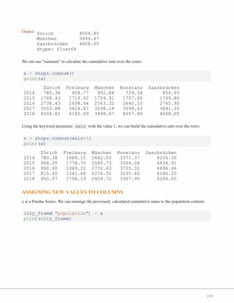
We can use "cumsum" to calculate the cumulative sum over the years:

x = shops.cumsum()print(x)

Using the keyword parameter axis with the value 1, we can build the cumulative sum over the rows:

x = shops.cumsum(axis=1)print(x)

ASSIGNING NEW VALUES TO COLUMNS

x is a Pandas Series. We can reassign the previously calculated cumulative sums to the population column:

city_frame["population"] = xprint(city_frame)

Output: Zürich 4504.85München 3999.67Saarbrücken 4608.05dtype: float64

Zürich Freiburg München Konstanz Saarbrücken2014 780.38 908.77 952.88 729.34 854.932015 1748.43 1719.42 1759.91 1707.65 1749.802016 2738.43 2698.64 2563.32 2640.33 2740.952017 3553.88 3424.87 3298.14 3599.63 3691.352018 4504.85 4182.09 3999.67 4557.86 4608.05

Zürich Freiburg München Konstanz Saarbrücken2014 780.38 1689.15 2642.03 3371.37 4226.302015 968.05 1778.70 2585.73 3564.04 4458.912016 990.00 1969.22 2772.63 3705.31 4696.462017 815.45 1541.68 2276.50 3235.80 4186.202018 950.97 1708.19 2409.72 3367.95 4284.65

330

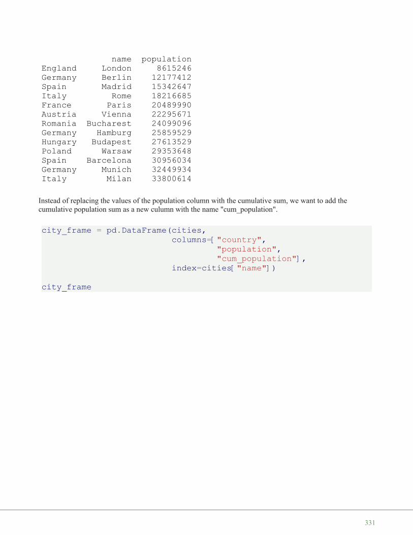
Instead of replacing the values of the population column with the cumulative sum, we want to add thecumulative population sum as a new culumn with the name "cum_population".

city_frame = pd.DataFrame(cities,columns=["country",

"population","cum_population"],

index=cities["name"])

city_frame

name populationEngland London 8615246Germany Berlin 12177412Spain Madrid 15342647Italy Rome 18216685France Paris 20489990Austria Vienna 22295671Romania Bucharest 24099096Germany Hamburg 25859529Hungary Budapest 27613529Poland Warsaw 29353648Spain Barcelona 30956034Germany Munich 32449934Italy Milan 33800614

331

We can see that the column "cum_population" is set to Nan, as we haven't provided any data for it.

We will assign now the cumulative sums to this column:

city_frame["cum_population"] = city_frame["population"].cumsum()city_frame

Output:

country population cum_population

London England 8615246 NaN

Berlin Germany 3562166 NaN

Madrid Spain 3165235 NaN

Rome Italy 2874038 NaN

Paris France 2273305 NaN

Vienna Austria 1805681 NaN

Bucharest Romania 1803425 NaN

Hamburg Germany 1760433 NaN

Budapest Hungary 1754000 NaN

Warsaw Poland 1740119 NaN

Barcelona Spain 1602386 NaN

Munich Germany 1493900 NaN

Milan Italy 1350680 NaN

332

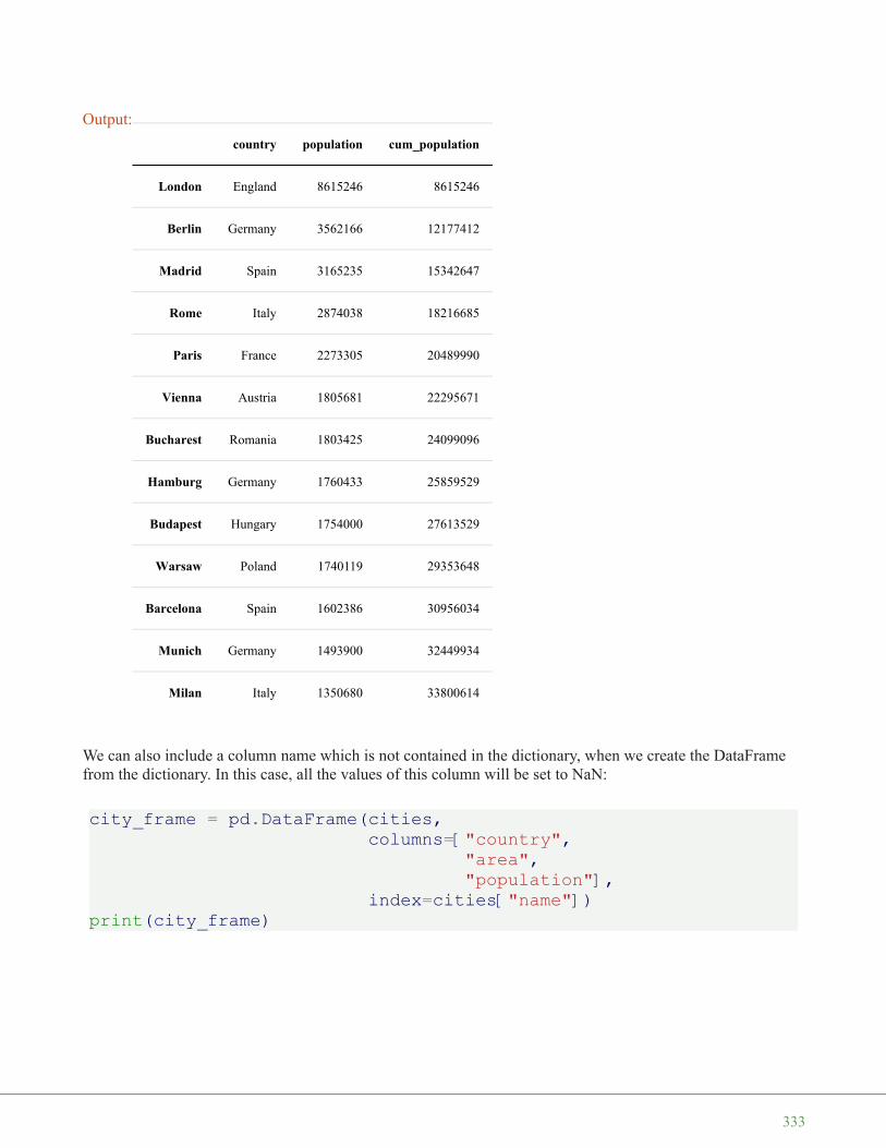
We can also include a column name which is not contained in the dictionary, when we create the DataFramefrom the dictionary. In this case, all the values of this column will be set to NaN:

city_frame = pd.DataFrame(cities,columns=["country",

"area","population"],

index=cities["name"])print(city_frame)

Output:

country population cum_population

London England 8615246 8615246

Berlin Germany 3562166 12177412

Madrid Spain 3165235 15342647

Rome Italy 2874038 18216685

Paris France 2273305 20489990

Vienna Austria 1805681 22295671

Bucharest Romania 1803425 24099096

Hamburg Germany 1760433 25859529

Budapest Hungary 1754000 27613529

Warsaw Poland 1740119 29353648

Barcelona Spain 1602386 30956034

Munich Germany 1493900 32449934

Milan Italy 1350680 33800614

333

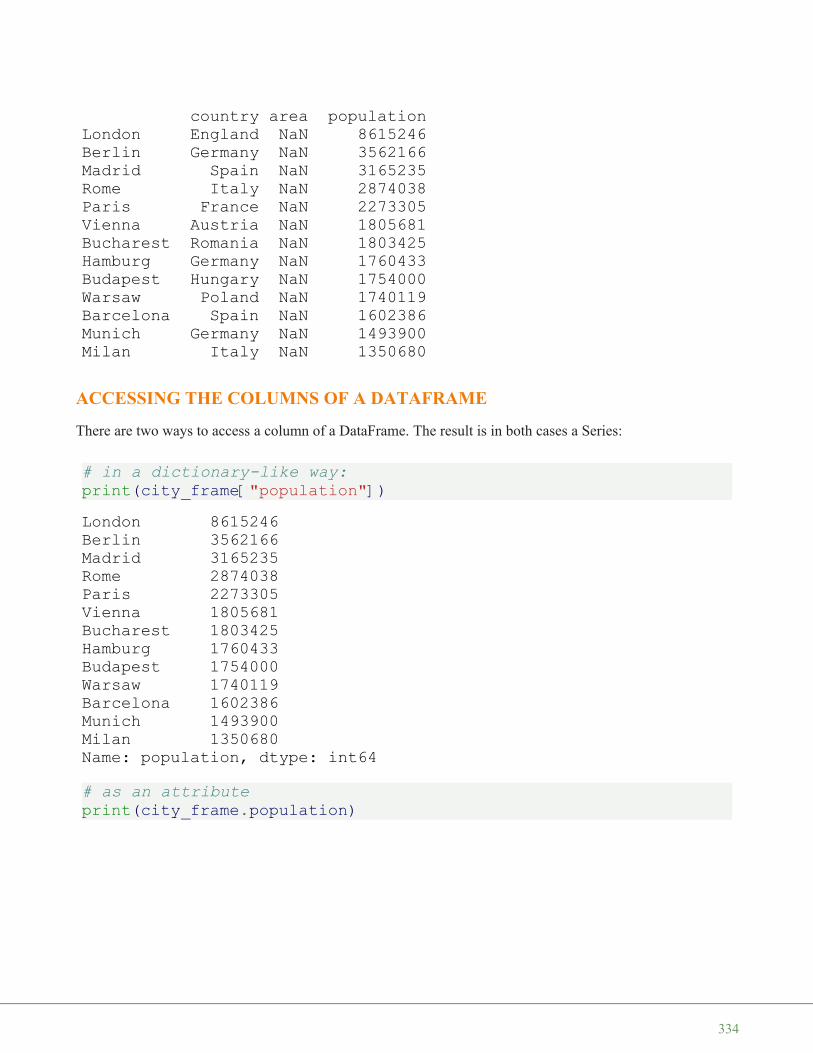
ACCESSING THE COLUMNS OF A DATAFRAME

There are two ways to access a column of a DataFrame. The result is in both cases a Series:

# in a dictionary-like way:print(city_frame["population"])

# as an attributeprint(city_frame.population)

country area populationLondon England NaN 8615246Berlin Germany NaN 3562166Madrid Spain NaN 3165235Rome Italy NaN 2874038Paris France NaN 2273305Vienna Austria NaN 1805681Bucharest Romania NaN 1803425Hamburg Germany NaN 1760433Budapest Hungary NaN 1754000Warsaw Poland NaN 1740119Barcelona Spain NaN 1602386Munich Germany NaN 1493900Milan Italy NaN 1350680

London 8615246Berlin 3562166Madrid 3165235Rome 2874038Paris 2273305Vienna 1805681Bucharest 1803425Hamburg 1760433Budapest 1754000Warsaw 1740119Barcelona 1602386Munich 1493900Milan 1350680Name: population, dtype: int64

334

print(type(city_frame.population))

city_frame.population

From the previous example, we can see that we have not copied the population column. "p" is a view on thedata of city_frame.

ASSIGNING NEW VALUES TO A COLUMN

The column area is still not defined. We can set all elements of the column to the same value:

city_frame["area"] = 1572print(city_frame)

London 8615246Berlin 3562166Madrid 3165235Rome 2874038Paris 2273305Vienna 1805681Bucharest 1803425Hamburg 1760433Budapest 1754000Warsaw 1740119Barcelona 1602386Munich 1493900Milan 1350680Name: population, dtype: int64

<class 'pandas.core.series.Series'>

Output: London 8615246Berlin 3562166Madrid 3165235Rome 2874038Paris 2273305Vienna 1805681Bucharest 1803425Hamburg 1760433Budapest 1754000Warsaw 1740119Barcelona 1602386Munich 1493900Milan 1350680Name: population, dtype: int64

335

In this case, it will be definitely better to assign the exact area to the cities. The list with the area values needsto have the same length as the number of rows in our DataFrame.

# area in square km:area = [1572, 891.85, 605.77, 1285,

105.4, 414.6, 228, 755,525.2, 517, 101.9, 310.4,181.8]

# area could have been designed as a list, a Series, an array ora scalar

city_frame["area"] = areaprint(city_frame)

country area populationLondon England 1572 8615246Berlin Germany 1572 3562166Madrid Spain 1572 3165235Rome Italy 1572 2874038Paris France 1572 2273305Vienna Austria 1572 1805681Bucharest Romania 1572 1803425Hamburg Germany 1572 1760433Budapest Hungary 1572 1754000Warsaw Poland 1572 1740119Barcelona Spain 1572 1602386Munich Germany 1572 1493900Milan Italy 1572 1350680

country area populationLondon England 1572.00 8615246Berlin Germany 891.85 3562166Madrid Spain 605.77 3165235Rome Italy 1285.00 2874038Paris France 105.40 2273305Vienna Austria 414.60 1805681Bucharest Romania 228.00 1803425Hamburg Germany 755.00 1760433Budapest Hungary 525.20 1754000Warsaw Poland 517.00 1740119Barcelona Spain 101.90 1602386Munich Germany 310.40 1493900Milan Italy 181.80 1350680

336

SORTING DATAFRAMES

Let's sort our DataFrame according to the city area:

city_frame = city_frame.sort_values(by="area", ascending=False)print(city_frame)

Let's assume, we have only the areas of London, Hamburg and Milan. The areas are in a series with the correctindices. We can assign this series as well:

city_frame = pd.DataFrame(cities,columns=["country",

"area","population"],

index=cities["name"])

some_areas = pd.Series([1572, 755, 181.8],index=['London', 'Hamburg', 'Milan'])

city_frame['area'] = some_areasprint(city_frame)

country area populationLondon England 1572.00 8615246Rome Italy 1285.00 2874038Berlin Germany 891.85 3562166Hamburg Germany 755.00 1760433Madrid Spain 605.77 3165235Budapest Hungary 525.20 1754000Warsaw Poland 517.00 1740119Vienna Austria 414.60 1805681Munich Germany 310.40 1493900Bucharest Romania 228.00 1803425Milan Italy 181.80 1350680Paris France 105.40 2273305Barcelona Spain 101.90 1602386

337

INSERTING NEW COLUMNS INTO EXISTING DATAFRAMES

In the previous example we have added the column area at creation time. Quite often it will be necessary toadd or insert columns into existing DataFrames. For this purpose the DataFrame class provides a method"insert", which allows us to insert a column into a DataFrame at a specified location:

insert(self, loc, column, value, allow_duplicates=False)`The parameters are specified as:

Parameter Meaning

loc int

This value should be withinthe range 0 <= loc <= len(columns)

column the column name

value can be a list, a Series an array or a scalar

allow_duplicates

If allow_duplicates is False,an Exception will be raised,

if column is already containedin the DataFrame.

city_frame = pd.DataFrame(cities,columns=["country",

"population"],index=cities["name"])

country area populationLondon England 1572.0 8615246Berlin Germany NaN 3562166Madrid Spain NaN 3165235Rome Italy NaN 2874038Paris France NaN 2273305Vienna Austria NaN 1805681Bucharest Romania NaN 1803425Hamburg Germany 755.0 1760433Budapest Hungary NaN 1754000Warsaw Poland NaN 1740119Barcelona Spain NaN 1602386Munich Germany NaN 1493900Milan Italy 181.8 1350680

338

idx = 1city_frame.insert(loc=idx, column='area', value=area)city_frame

CREATING A DATAFRAME BY APPENDING ROWSimport pandas as pdfrom numpy.random import randint

df = pd.DataFrame(columns=['lib', 'qty1', 'qty2'])for i in range(5):

df.loc[i] = ['name' + str(i)] + list(randint(10, size=2))

Output:

country area population

London England 1572.00 8615246

Berlin Germany 891.85 3562166

Madrid Spain 605.77 3165235

Rome Italy 1285.00 2874038

Paris France 105.40 2273305

Vienna Austria 414.60 1805681

Bucharest Romania 228.00 1803425

Hamburg Germany 755.00 1760433

Budapest Hungary 525.20 1754000

Warsaw Poland 517.00 1740119

Barcelona Spain 101.90 1602386

Munich Germany 310.40 1493900

Milan Italy 181.80 1350680

339

df

DATAFRAME FROM NESTED DICTIONARIES

A nested dictionary of dicts can be passed to a DataFrame as well. The indices of the outer dictionary aretaken as the the columns and the inner keys. i.e. the keys of the nested dictionaries, are used as the rowindices:

growth = {"Switzerland": {"2010": 3.0, "2011": 1.8, "2012": 1.1,"2013": 1.9},

"Germany": {"2010": 4.1, "2011": 3.6, "2012":0.4, "2013": 0.1},

"France": {"2010":2.0, "2011":2.1, "2012": 0.3, "2013": 0.3},

"Greece": {"2010":-5.4, "2011":-8.9, "2012":-6.6, "2013": -3.3},

"Italy": {"2010":1.7, "2011": 0.6, "2012":-2.3,"2013":-1.9}

}growth_frame = pd.DataFrame(growth)growth_frame

Output:

lib qty1 qty2

0 name0 1 8

1 name1 5 6

2 name2 9 9

3 name3 8 8

4 name4 7 0

340

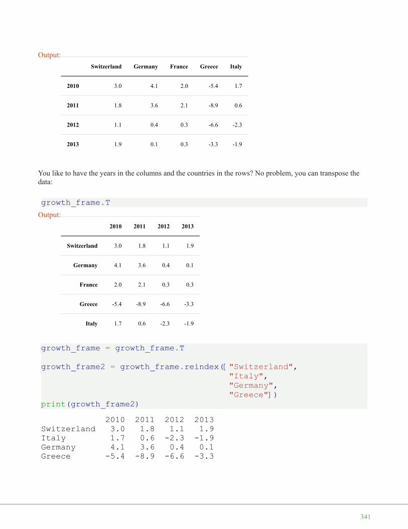
You like to have the years in the columns and the countries in the rows? No problem, you can transpose thedata:

growth_frame.T

growth_frame = growth_frame.T

growth_frame2 = growth_frame.reindex(["Switzerland","Italy","Germany","Greece"])

print(growth_frame2)

Output:

Switzerland Germany France Greece Italy

2010 3.0 4.1 2.0 -5.4 1.7

2011 1.8 3.6 2.1 -8.9 0.6

2012 1.1 0.4 0.3 -6.6 -2.3

2013 1.9 0.1 0.3 -3.3 -1.9

Output:

2010 2011 2012 2013

Switzerland 3.0 1.8 1.1 1.9

Germany 4.1 3.6 0.4 0.1

France 2.0 2.1 0.3 0.3

Greece -5.4 -8.9 -6.6 -3.3

Italy 1.7 0.6 -2.3 -1.9

2010 2011 2012 2013Switzerland 3.0 1.8 1.1 1.9Italy 1.7 0.6 -2.3 -1.9Germany 4.1 3.6 0.4 0.1Greece -5.4 -8.9 -6.6 -3.3

341

FILLING A DATAFRAME WITH RANDOM VALUES:import numpy as npnames = ['Frank', 'Eve', 'Stella', 'Guido', 'Lara']index = ["January", "February", "March",

"April", "May", "June","July", "August", "September","October", "November", "December"]

df = pd.DataFrame((np.random.randn(12, 5)*1000).round(2),columns=names,index=index)

dfOutput:

Frank Eve Stella Guido Lara

January -2452.01 -91.03 -122.31 -750.05 931.99

February -874.08 -189.72 628.49 -392.53 342.06

March -1222.37 -1125.60 -826.90 -107.74 -831.32

April 1333.69 1468.56 -1537.82 -743.23 624.10

May 802.27 -1444.17 84.38 -376.80 256.64

June -762.07 207.63 -476.06 -2068.54 -1614.25

July -1172.28 -2582.39 -351.16 -555.88 -21.40

August -468.52 -665.97 833.53 -1650.37 -426.07

September -788.57 408.96 -652.73 346.99 875.78

October 92.81 699.84 251.47 872.04 415.53

November 558.65 -1699.90 -949.95 212.92 -1874.80

December -646.58 -35.22 -1018.20 -644.35 776.56

342

A C C E S S I N G A N D C H A N G I N G V A L U E S O FD A T A F R A M E S

We have seen in the previous chapters of our tutorial manyways to create Series and DataFrames. We also learnedhow to access and replace complete columns. This chapterof our Pandas and Python tutorial will show various waysto access and change selectively values in PandasDataFrames and Series. We will show ways how to changesingle value or values matching strings or regularexpressions.

For this purpose we will learn to know the methods loc ,at and replace

We will work with the following DataFrame structure inour examples:

import pandas as pdfirst = ('Mike', 'Dorothee', 'Tom', 'Bill', 'Pete', 'Kate')last = ('Meyer', 'Maier', 'Meyer', 'Mayer', 'Meyr', 'Mair')job = ('data analyst', 'programmer', 'computer scientist',

'data scientist', 'accountant', 'psychiatrist')language = ('Python', 'Perl', 'Java', 'Java', 'Cobol', 'Brainfuck')

df = pd.DataFrame(list(zip(last, job, language)),columns =['last', 'job', 'language'],index=first)

df

343

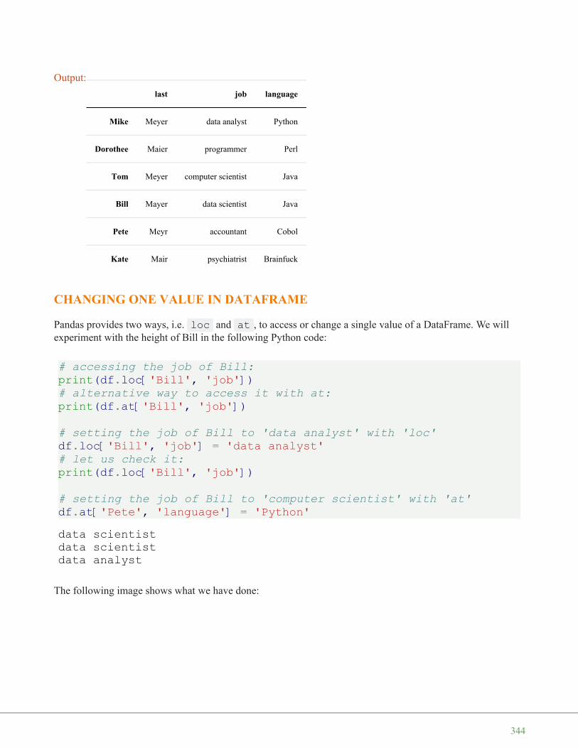
CHANGING ONE VALUE IN DATAFRAME

Pandas provides two ways, i.e. loc and at , to access or change a single value of a DataFrame. We willexperiment with the height of Bill in the following Python code:

# accessing the job of Bill:print(df.loc['Bill', 'job'])# alternative way to access it with at:print(df.at['Bill', 'job'])

# setting the job of Bill to 'data analyst' with 'loc'df.loc['Bill', 'job'] = 'data analyst'# let us check it:print(df.loc['Bill', 'job'])

# setting the job of Bill to 'computer scientist' with 'at'df.at['Pete', 'language'] = 'Python'

The following image shows what we have done:

Output:

last job language

Mike Meyer data analyst Python

Dorothee Maier programmer Perl

Tom Meyer computer scientist Java

Bill Mayer data scientist Java

Pete Meyr accountant Cobol

Kate Mair psychiatrist Brainfuck

data scientistdata scientistdata analyst

344

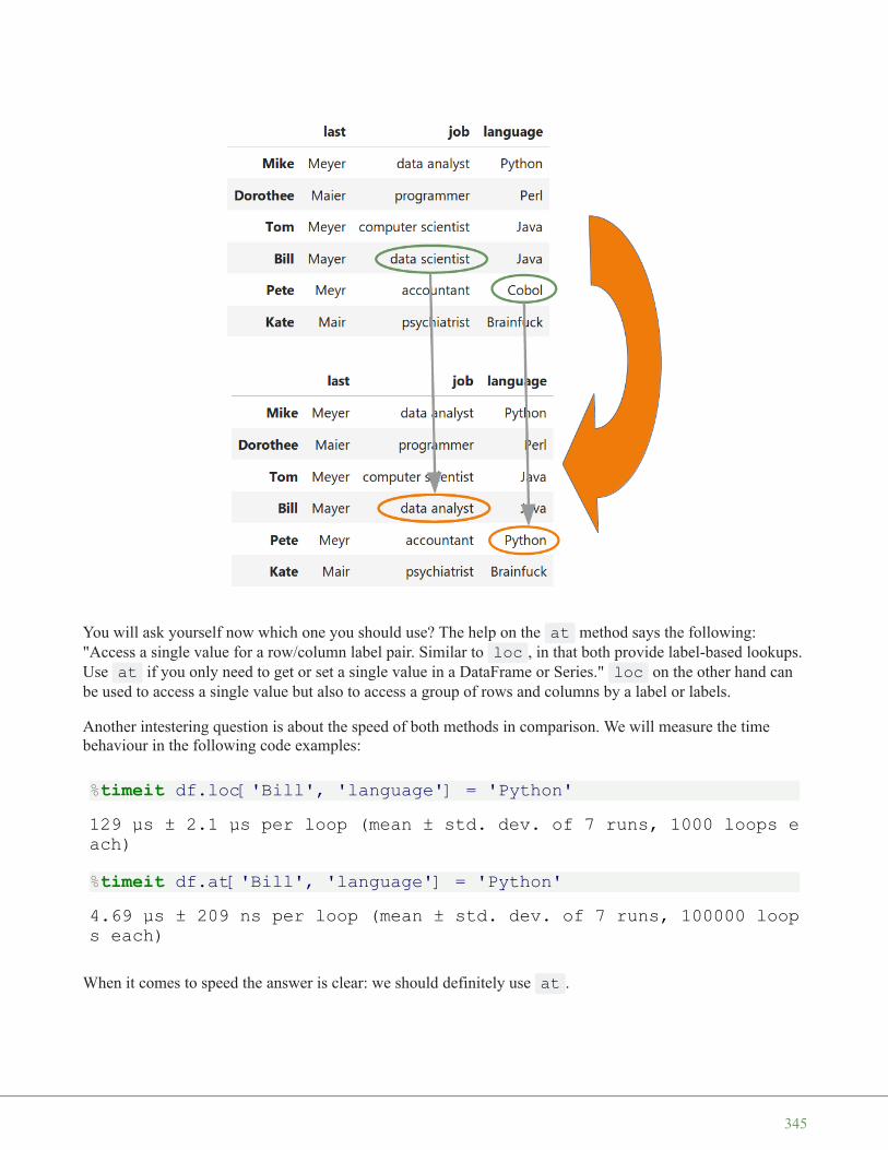
You will ask yourself now which one you should use? The help on the at method says the following:"Access a single value for a row/column label pair. Similar to loc , in that both provide label-based lookups.Use at if you only need to get or set a single value in a DataFrame or Series." loc on the other hand canbe used to access a single value but also to access a group of rows and columns by a label or labels.

Another intestering question is about the speed of both methods in comparison. We will measure the timebehaviour in the following code examples:

%timeit df.loc['Bill', 'language'] = 'Python'

%timeit df.at['Bill', 'language'] = 'Python'

When it comes to speed the answer is clear: we should definitely use at .

129 µs ± 2.1 µs per loop (mean ± std. dev. of 7 runs, 1000 loops each)

4.69 µs ± 209 ns per loop (mean ± std. dev. of 7 runs, 100000 loops each)

345

REPLACE

The syntax of replace :

replace(self,to_replace=None,value=None,inplace=False,limit=None,regex=False,method='pad')

This method replaces values given in to_replace with value . This differs from updating with .locor .iloc , which requires you to specify a location to update with some value. With replace it is possible toreplace values in a Series or DataFrame without knowing where they occur.

replace works both with Series and DataFrames.

We will explain the way of working of the method replace by discussing the different data types of theparameter to_replace individually:

TO_REPLACE CAN BE NUMERIC VALUE, STRING OR REGULAREXPRESSION:

DataType processing

numericnumeric values in the DataFrame (or Series) which are equal to to_replace will be replaced with parameter

value

strIf the parameter to_replace consists of a string, all the strings of the DataFrame (or Series) which exactly match

this string will be replaced by the value of the parameter value

regexAll strings inside of the DataFrame (or Series) which match the regular expression of to_replace will be replaced

with value

Let's start with a Series example. We will change one value into another one. Be aware of the fact thatreplace by default creates a copy of the object in which all the values are replaced. This means that the

parameter inplace is set to False by default.

s = pd.Series([27, 33, 13, 19])s.replace(13, 42)

346

If we really want to change the object s is referencing, we should set the inplace parameter to True :

s = pd.Series([27, 33, 13, 19])s.replace(13, 42, inplace=True)s

We can also change multiple values into one single value, as you can see in the following example.

s = pd.Series([0, 1, 2, 3, 4])s.replace([0, 1, 2], 42, inplace=True)s

We will show now, how replace can be used on DataFrames. For this purpose we will recreate the examplefrom the beginning of this chapter of our tutorial. It will not be exactly the same though. More people havelearned Python now, but unfortunately somebody has put in some spelling errors in the word Python. Pete hasbecome a programmer now:

import pandas as pdfirst = ('Mike', 'Dorothee', 'Tom', 'Bill', 'Pete', 'Kate')last = ('Meyer', 'Maier', 'Meyer', 'Mayer', 'Meyr', 'Mair')job = ('data analyst', 'programmer', 'computer scientist',

'data scientist', 'programmer', 'psychiatrist')language = ('Python', 'Perl', 'Java', 'Pithon', 'Pythen', 'Brainfuck')

Output: 0 271 332 423 19dtype: int64

Output: 0 271 332 423 19dtype: int64

Output: 0 421 422 423 34 4dtype: int64

347

df = pd.DataFrame(list(zip(last, job, language)),columns =['last', 'job', 'language'],index=first)

df

Both ambitious Dorothee and enthusiastic Pete have finished a degree in Computer Science in the meantime.So we have to change our DataFrame accodingly:

df.replace("programmer","computer scientist",inplace=True)

df

Output:

last job language

Mike Meyer data analyst Python

Dorothee Maier programmer Perl

Tom Meyer computer scientist Java

Bill Mayer data scientist Pithon

Pete Meyr programmer Pythen

Kate Mair psychiatrist Brainfuck

348

TO_REPLACE CAN BE A LIST CONSISTING OF STR, REGEX OR NUMERICOBJECTS:

to_replace can be a list consisting of str, regex or numeric objects. If both the values of to_replaceand value are both lists, they must be the same length.

First, if to_replace and value are both lists, they must be the same length. Second, ifregex=True then all of the strings in both lists will be interpreted as regexs otherwise they will match

directly. We slightly changed our DataFrame for the next example. The first names build a column now!

df = pd.DataFrame(list(zip(first, last, job, language)),columns =['first', 'last', 'job', 'language'])

df

Output:

last job language

Mike Meyer data analyst Python

Dorothee Maier computer scientist Perl

Tom Meyer computer scientist Java

Bill Mayer data scientist Pithon

Pete Meyr computer scientist Pythen

Kate Mair psychiatrist Brainfuck

Output:

first last job language

0 Mike Meyer data analyst Python

1 Dorothee Maier programmer Perl

2 Tom Meyer computer scientist Java

3 Bill Mayer data scientist Pithon

4 Pete Meyr programmer Pythen

5 Kate Mair psychiatrist Brainfuck

349

'Mike' and 'Tom' are abbreviations of the real first names, so we will change them now. We are also glad toannounce that Dorothee finally migrated from Perl to Python:

df.replace(to_replace=['Mike', 'Tom', 'Perl'],value= ['Michael', 'Thomas', 'Python'],inplace=True)

df

USING REGULAR EXPRESSIONS

Now it is time to do something about the surnames in our DataFrame. All these names sound the same - atleast for German speakers. Let us assume that we just found out that they should all be spelled the same, i.e.Mayer. Now the time has come for regular expression. The parameter to_replace can also be used withregular expressions. We will use a regular expression to unify the surnames. We will also fix the misspellingsof Python:

df.replace(to_replace=[r'M[ea][iy]e?r', r'P[iy]th[eo]n'],value=['Mayer', 'Python'],regex=True,inplace=True)

df

Output:

first last job language

0 Michael Meyer data analyst Python

1 Dorothee Maier programmer Python

2 Thomas Meyer computer scientist Java

3 Bill Mayer data scientist Pithon

4 Pete Meyr programmer Pythen

5 Kate Mair psychiatrist Brainfuck

350

TO_REPLACE CAN BE A DICT

Dictionaries can be used to specify different replacement values for different existing values. For example,{'a': 'b', 'y': 'z'} replaces the value 'a' with 'b' and 'y' with 'z'. To use a dict in this way thevalue parameter should be None .

Ìf replace is applied on a DataFrame, a dict can specify that different values should be replaced indifferent columns. For example, {'a': 1, 'b': 'z'} looks for the value 1 in column 'a' and the value'z' in column 'b' and replaces these values with whatever is specified in value . The value parametershould not be None in this case. You can treat this as a special case of passing two lists except that you arespecifying the column to search in.

If we use nested dictionaries like {'A': {'foo': 'bar'}} , they are interpreted like this: look incolumn 'A' for the value 'foo' and replace it with 'bar'. The value parameter has to be None in this case.

df = pd.DataFrame({'A': [0, 1, 2, 3, 4],'B': ['foo', 'bar', 'bloo', 'blee', 'bloo'],'C': ['green', 'red', 'blue', 'yellow', 'gree

n']})

df.replace(to_replace={"A": {0: 42, 3: 33}, 'B': {'bloo': 'vloo'}},

inplace=True)df

Output:

first last job language

0 Michael Mayer data analyst Python

1 Dorothee Mayer programmer Python

2 Thomas Mayer computer scientist Java

3 Bill Mayer data scientist Python

4 Pete Mayer programmer Python

5 Kate Mayer psychiatrist Brainfuck

351

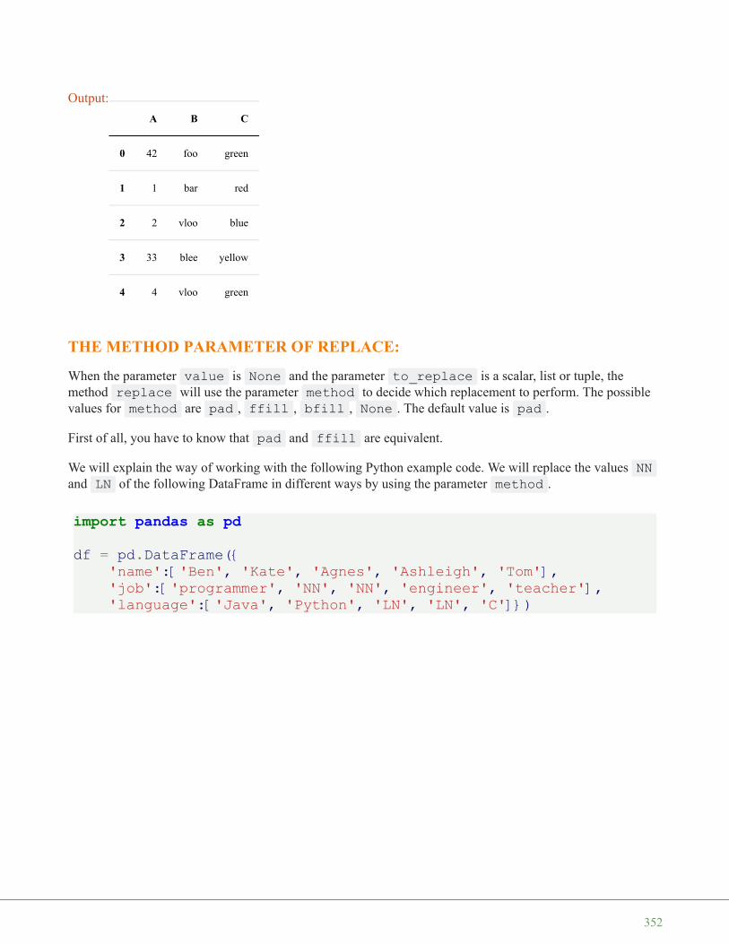
THE METHOD PARAMETER OF REPLACE:

When the parameter value is None and the parameter to_replace is a scalar, list or tuple, themethod replace will use the parameter method to decide which replacement to perform. The possiblevalues for method are pad , ffill , bfill , None . The default value is pad .

First of all, you have to know that pad and ffill are equivalent.

We will explain the way of working with the following Python example code. We will replace the values NNand LN of the following DataFrame in different ways by using the parameter method .

import pandas as pddf = pd.DataFrame({

'name':['Ben', 'Kate', 'Agnes', 'Ashleigh', 'Tom'],'job':['programmer', 'NN', 'NN', 'engineer', 'teacher'],'language':['Java', 'Python', 'LN', 'LN', 'C']})

Output:

A B C

0 42 foo green

1 1 bar red

2 2 vloo blue

3 33 blee yellow

4 4 vloo green

352

We will start with changing the 'NN' values by using ffill in the parameter method :

The picture above shows how the following call to replace . In words: Every occurrence of NN in thejob column will have to be replaced. The value is defined by the parameter method . ffill means

'forward fill', i.e. we will take the preceding value to the first NN as the fill value. This is why we will replacethe values by 'programmer':

# method is backfilldf.replace(to_replace='NN',

value=None,method='ffill')

353

Instead of using a single value for to_replace we can also use a list or tuple. We will replace in thefollowing all occurrences of NN and LN accordingly, as we can see in the following picture:

df.replace(to_replace=['NN', 'LN'],value=None,method='ffill')

Output:

name job language

0 Ben programmer Java

1 Kate programmer Python

2 Agnes programmer LN

3 Ashleigh engineer LN

4 Tom teacher C

354

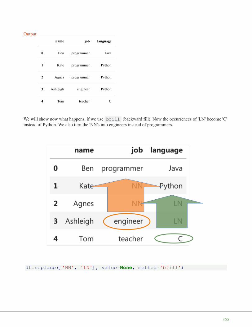
We will show now what happens, if we use bfill (backward fill). Now the occurrences of 'LN' become 'C'instead of Python. We also turn the 'NN's into engineers instead of programmers.

df.replace(['NN', 'LN'], value=None, method='bfill')

Output:

name job language

0 Ben programmer Java

1 Kate programmer Python

2 Agnes programmer Python

3 Ashleigh engineer Python

4 Tom teacher C

355

df.replace('NN',value=None,inplace=True,method='bfill')

df.replace('LN',value=None,inplace=True,method='ffill')

df

OTHER EXAMPLES

We will present some more examples, which are taken from the help file of loc :

df = pd.DataFrame([[1, 2], [4, 5], [7, 8]],index=['cobra', 'viper', 'sidewinder'],columns=['max_speed', 'shield'])

Output:

name job language

0 Ben programmer Java

1 Kate engineer Python

2 Agnes engineer C

3 Ashleigh engineer C

4 Tom teacher C

Output:

name job language

0 Ben programmer Java

1 Kate engineer Python

2 Agnes engineer Python

3 Ashleigh engineer Python

4 Tom teacher C

356

df

Single label. Note this returns the row as a Series:

df.loc['viper']

List of labels. Note using [[]] returns a DataFrame:

df.loc[['viper', 'sidewinder']]

Single label for row and column

df.loc['cobra', 'shield']

Slice with labels for row and single label for column. As mentioned above, note that both the start and stop ofthe slice are included.

df.loc['cobra':'viper', 'max_speed']

Output:

max_speed shield

cobra 1 2

viper 4 5

sidewinder 7 8

Output: max_speed 4shield 5Name: viper, dtype: int64

Output:

max_speed shield

viper 4 5

sidewinder 7 8

Output: 2

357

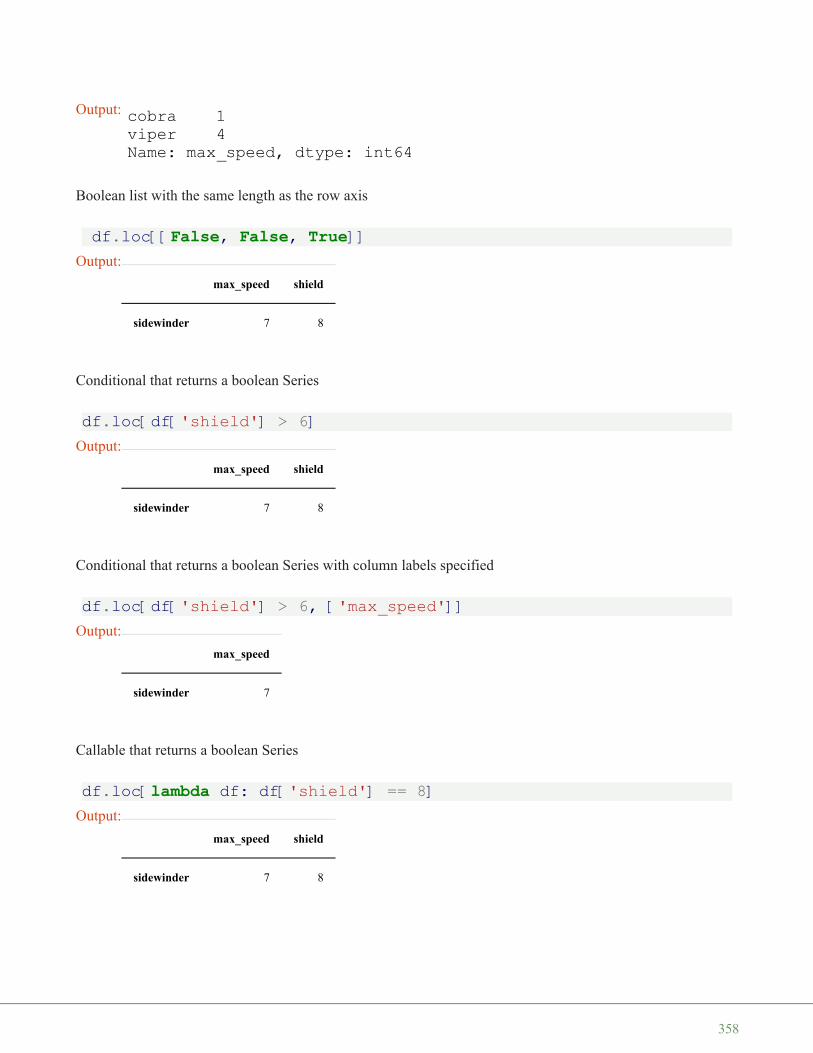
Boolean list with the same length as the row axis

df.loc[[False, False, True]]

Conditional that returns a boolean Series

df.loc[df['shield'] > 6]

Conditional that returns a boolean Series with column labels specified

df.loc[df['shield'] > 6, ['max_speed']]

Callable that returns a boolean Series

df.loc[lambda df: df['shield'] == 8]

Output: cobra 1viper 4Name: max_speed, dtype: int64

Output:

max_speed shield

sidewinder 7 8

Output:

max_speed shield

sidewinder 7 8

Output:

max_speed

sidewinder 7

Output:

max_speed shield

sidewinder 7 8

358

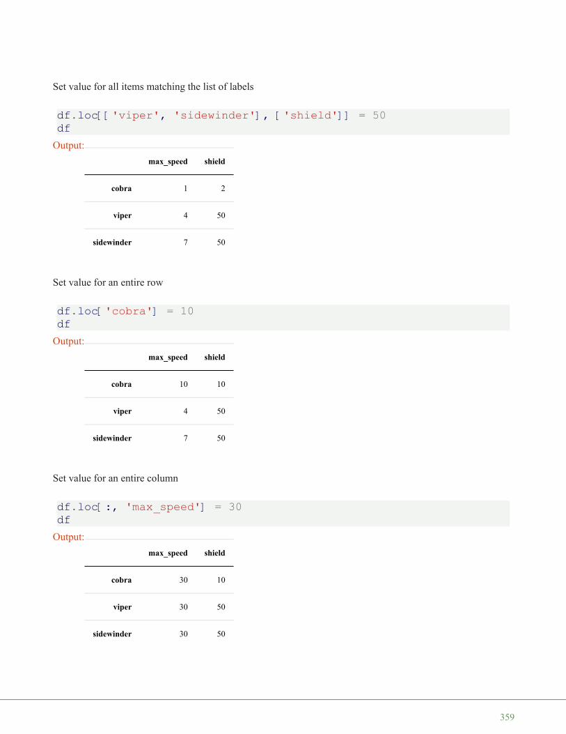
Set value for all items matching the list of labels

df.loc[['viper', 'sidewinder'], ['shield']] = 50df

Set value for an entire row

df.loc['cobra'] = 10df

Set value for an entire column

df.loc[:, 'max_speed'] = 30df

Output:

max_speed shield

cobra 1 2

viper 4 50

sidewinder 7 50

Output:

max_speed shield

cobra 10 10

viper 4 50

sidewinder 7 50

Output:

max_speed shield

cobra 30 10

viper 30 50

sidewinder 30 50

359

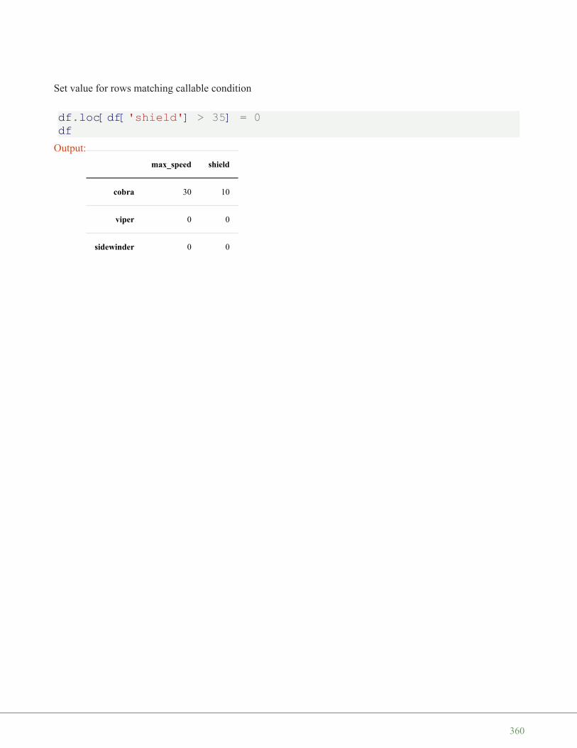
Set value for rows matching callable condition

df.loc[df['shield'] > 35] = 0df

Output:

max_speed shield

cobra 30 10

viper 0 0

sidewinder 0 0

360

P A N D A S : G R O U P B Y

This chapter of our Pandas tutorial deals with an extremelyimportant functionality, i.e. groupby . It is not reallycomplicated, but it is not obvious at first glance and issometimes found to be difficult. Completely wrong, as weshall see. It is also very important to become familiar with'groupby' because it can be used to solve importantproblems that would not be possible without it. ThePandas groupby operation involves some combinationof splitting the object, applying a function, and combiningthe results. We can split a DataFrame object into groupsbased on various criteria and row and column-wise, i.e.using axis .

'Applying' means

• to filter the data,• transform the data or• aggregate the data.

groupby can be applied to Pandas Series objects andDataFrame objects! We will learn to understand how it works with many small practical examples in thistutorial.

GOUPBY WITH SERIES

We create with the following Python program a Series object with an index of size nvalues . The indexwill not be unique, because the strings for the index are taken from the list fruits , which has less elementsthan nvalues :

import pandas as pdimport numpy as npimport randomnvalues = 30# we create random values, which will be used as the Series values:values = np.random.randint(1, 20, (nvalues,))fruits = ["bananas", "oranges", "apples", "clementines", "cherries", "pears"]fruits_index = np.random.choice(fruits, (nvalues,))

s = pd.Series(values, index=fruits_index)

361

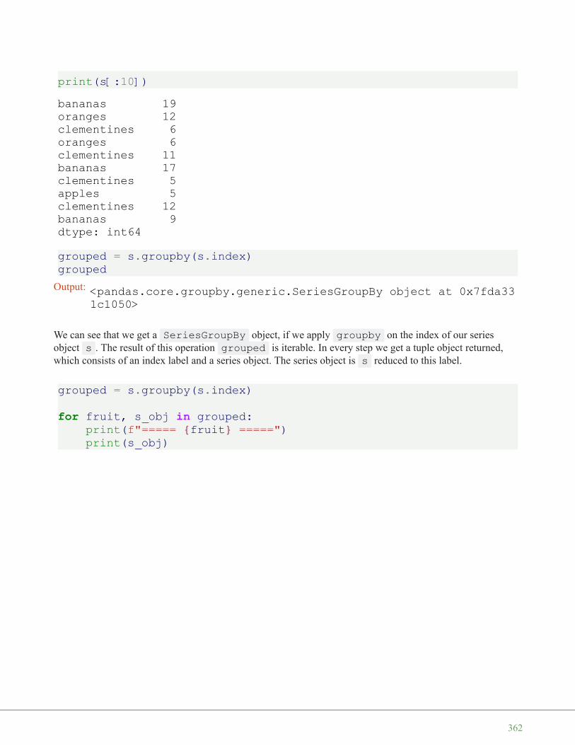
print(s[:10])

grouped = s.groupby(s.index)grouped

We can see that we get a SeriesGroupBy object, if we apply groupby on the index of our seriesobject s . The result of this operation grouped is iterable. In every step we get a tuple object returned,which consists of an index label and a series object. The series object is s reduced to this label.

grouped = s.groupby(s.index)

for fruit, s_obj in grouped:print(f"===== {fruit} =====")print(s_obj)

bananas 19oranges 12clementines 6oranges 6clementines 11bananas 17clementines 5apples 5clementines 12bananas 9dtype: int64

Output: <pandas.core.groupby.generic.SeriesGroupBy object at 0x7fda331c1050>

362

We could have got the same result - except for the order - without using `` groupby '' with the followingPython code.

===== apples =====apples 5apples 17apples 9apples 16apples 9dtype: int64===== bananas =====bananas 19bananas 17bananas 9bananas 13bananas 7bananas 16bananas 11bananas 18bananas 13dtype: int64===== cherries =====cherries 12dtype: int64===== clementines =====clementines 6clementines 11clementines 5clementines 12clementines 12clementines 6dtype: int64===== oranges =====oranges 12oranges 6oranges 9dtype: int64===== pears =====pears 18pears 9pears 10pears 10pears 1pears 16dtype: int64

363

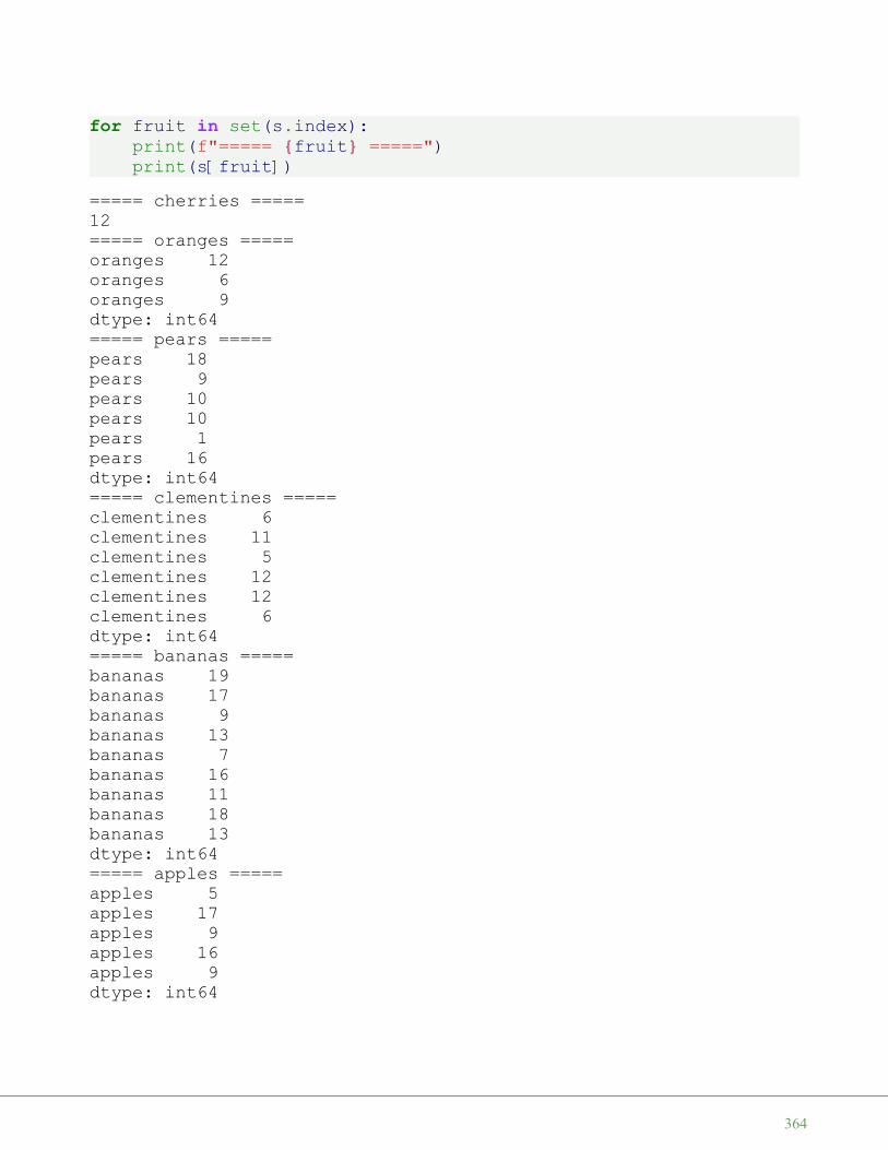
for fruit in set(s.index):print(f"===== {fruit} =====")print(s[fruit])

===== cherries =====12===== oranges =====oranges 12oranges 6oranges 9dtype: int64===== pears =====pears 18pears 9pears 10pears 10pears 1pears 16dtype: int64===== clementines =====clementines 6clementines 11clementines 5clementines 12clementines 12clementines 6dtype: int64===== bananas =====bananas 19bananas 17bananas 9bananas 13bananas 7bananas 16bananas 11bananas 18bananas 13dtype: int64===== apples =====apples 5apples 17apples 9apples 16apples 9dtype: int64

364

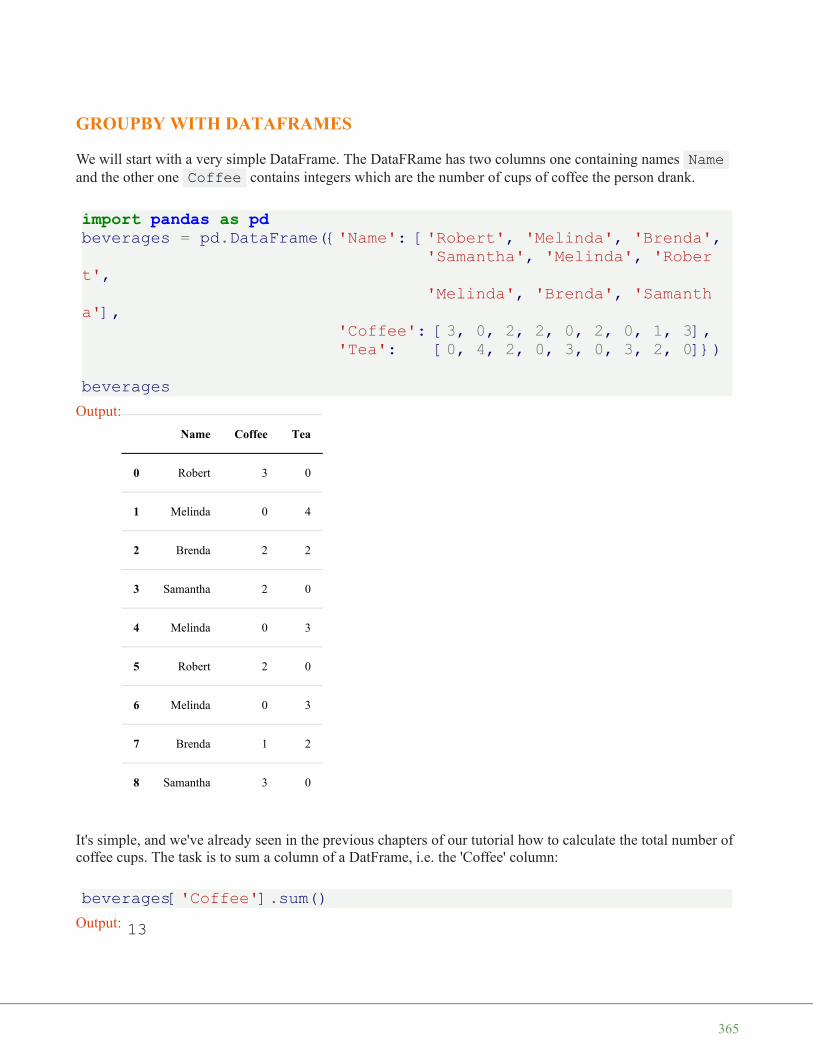
GROUPBY WITH DATAFRAMES

We will start with a very simple DataFrame. The DataFRame has two columns one containing names Nameand the other one Coffee contains integers which are the number of cups of coffee the person drank.

import pandas as pdbeverages = pd.DataFrame({'Name': ['Robert', 'Melinda', 'Brenda',

'Samantha', 'Melinda', 'Robert',

'Melinda', 'Brenda', 'Samantha'],

'Coffee': [3, 0, 2, 2, 0, 2, 0, 1, 3],'Tea': [0, 4, 2, 0, 3, 0, 3, 2, 0]})

beverages

It's simple, and we've already seen in the previous chapters of our tutorial how to calculate the total number ofcoffee cups. The task is to sum a column of a DatFrame, i.e. the 'Coffee' column:

beverages['Coffee'].sum()

Output:

Name Coffee Tea

0 Robert 3 0

1 Melinda 0 4

2 Brenda 2 2

3 Samantha 2 0

4 Melinda 0 3

5 Robert 2 0

6 Melinda 0 3

7 Brenda 1 2

8 Samantha 3 0

Output: 13

365

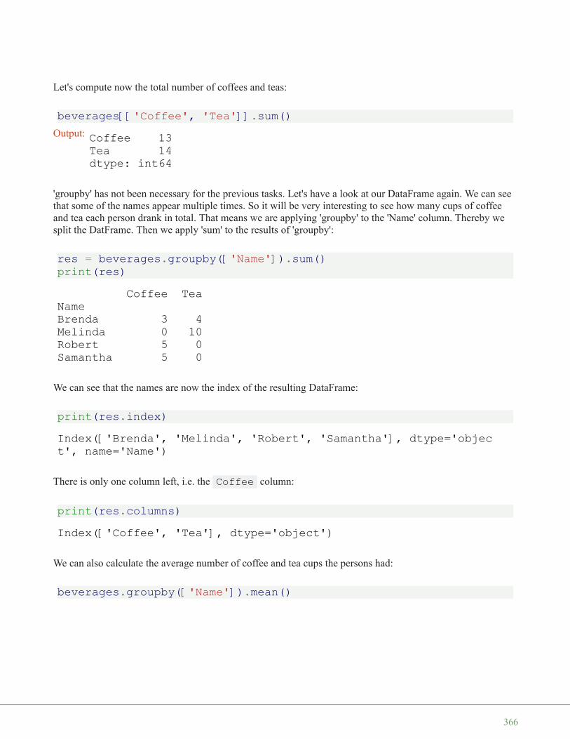
Let's compute now the total number of coffees and teas:

beverages[['Coffee', 'Tea']].sum()

'groupby' has not been necessary for the previous tasks. Let's have a look at our DataFrame again. We can seethat some of the names appear multiple times. So it will be very interesting to see how many cups of coffeeand tea each person drank in total. That means we are applying 'groupby' to the 'Name' column. Thereby wesplit the DatFrame. Then we apply 'sum' to the results of 'groupby':

res = beverages.groupby(['Name']).sum()print(res)

We can see that the names are now the index of the resulting DataFrame:

print(res.index)

There is only one column left, i.e. the Coffee column:

print(res.columns)

We can also calculate the average number of coffee and tea cups the persons had:

beverages.groupby(['Name']).mean()

Output: Coffee 13Tea 14dtype: int64

Coffee TeaNameBrenda 3 4Melinda 0 10Robert 5 0Samantha 5 0

Index(['Brenda', 'Melinda', 'Robert', 'Samantha'], dtype='object', name='Name')

Index(['Coffee', 'Tea'], dtype='object')

366

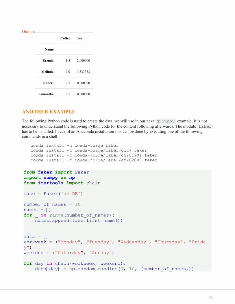
ANOTHER EXAMPLE

The following Python code is used to create the data, we will use in our next groupby example. It is notnecessary to understand the following Python code for the content following afterwards. The module fakerhas to be installed. In cae of an Anaconda installation this can be done by executing one of the followingcommands in a shell:

conda install -c conda-forge fakerconda install -c conda-forge/label/gcc7 fakerconda install -c conda-forge/label/cf201901 fakerconda install -c conda-forge/label/cf202003 faker

from faker import Fakerimport numpy as npfrom itertools import chain

fake = Faker('de_DE')

number_of_names = 10names = []for _ in range(number_of_names):

names.append(fake.first_name())

data = {}workweek = ("Monday", "Tuesday", "Wednesday", "Thursday", "Friday")weekend = ("Saturday", "Sunday")

for day in chain(workweek, weekend):data[day] = np.random.randint(0, 10, (number_of_names,))

Output:

Coffee Tea

Name

Brenda 1.5 2.000000

Melinda 0.0 3.333333

Robert 2.5 0.000000

Samantha 2.5 0.000000

367

data_df = pd.DataFrame(data, index=names)data_df

print(names)

names = ('Ortwin', 'Mara', 'Siegrun', 'Sylvester', 'Metin', 'Adeline', 'Utz', 'Susan', 'Gisbert', 'Senol')data = {'Monday': np.array([0, 9, 2, 3, 7, 3, 9, 2, 4, 9]),

'Tuesday': np.array([2, 6, 3, 3, 5, 5, 7, 7, 1, 0]),'Wednesday': np.array([6, 1, 1, 9, 4, 0, 8, 6, 8, 8]),'Thursday': np.array([1, 8, 6, 9, 9, 4, 1, 7, 3, 2]),'Friday': np.array([3, 5, 6, 6, 5, 2, 2, 4, 6, 5]),'Saturday': np.array([8, 4, 8, 2, 3, 9, 3, 4, 9, 7]),'Sunday': np.array([0, 8, 7, 8, 9, 7, 2, 0, 5, 2])}

data_df = pd.DataFrame(data, index=names)data_df

Output:

Monday Tuesday Wednesday Thursday Friday Saturday Sunday

Kenan 0 0 5 9 2 2 9

Jovan 9 1 5 1 0 0 0

Stanislaus 6 7 5 1 1 5 3

Adelinde 2 2 5 8 7 4 9

Cengiz 2 7 3 8 4 6 9

Edeltraud 4 7 9 9 7 9 7

Sara 7 1 7 0 7 8 3

Gerda 9 8 7 0 8 5 8

Tilman 5 1 9 4 7 5 5

Roswita 1 8 5 3 5 3 9

['Kenan', 'Jovan', 'Stanislaus', 'Adelinde', 'Cengiz', 'Edeltraud', 'Sara', 'Gerda', 'Tilman', 'Roswita']

368

We will demonstrate with this DataFrame how to combine columns by a function.

def is_weekend(day):if day in {'Saturday', 'Sunday'}:

return "Weekend"else:

return "Workday"

for res_func, df in data_df.groupby(by=is_weekend, axis=1):print(df)

Output:

Monday Tuesday Wednesday Thursday Friday Saturday Sunday

Ortwin 0 2 6 1 3 8 0

Mara 9 6 1 8 5 4 8

Siegrun 2 3 1 6 6 8 7

Sylvester 3 3 9 9 6 2 8

Metin 7 5 4 9 5 3 9

Adeline 3 5 0 4 2 9 7

Utz 9 7 8 1 2 3 2

Susan 2 7 6 7 4 4 0

Gisbert 4 1 8 3 6 9 5

Senol 9 0 8 2 5 7 2

369

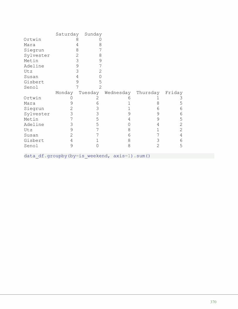
data_df.groupby(by=is_weekend, axis=1).sum()

Saturday SundayOrtwin 8 0Mara 4 8Siegrun 8 7Sylvester 2 8Metin 3 9Adeline 9 7Utz 3 2Susan 4 0Gisbert 9 5Senol 7 2

Monday Tuesday Wednesday Thursday FridayOrtwin 0 2 6 1 3Mara 9 6 1 8 5Siegrun 2 3 1 6 6Sylvester 3 3 9 9 6Metin 7 5 4 9 5Adeline 3 5 0 4 2Utz 9 7 8 1 2Susan 2 7 6 7 4Gisbert 4 1 8 3 6Senol 9 0 8 2 5

370

EXERCISES

EXERCISE 1

Calculate the average prices of the products of the following DataFrame:

import pandas as pdd = {"products": ["Oppilume", "Dreaker", "Lotadilo",

"Crosteron", "Wazzasoft", "Oppilume","Dreaker", "Lotadilo", "Wazzasoft"],

"colours": ["blue", "blue", "blue","green", "blue", "green","green", "green", "red"],

"customer_price": [2345.89, 2390.50, 1820.00,3100.00, 1784.50, 2545.89,2590.50, 2220.00, 2084.50],

"non_customer_price": [2445.89, 2495.50, 1980.00,3400.00, 1921.00, 2645.89,

Output:

Weekend Workday

Ortwin 8 12

Mara 12 29

Siegrun 15 18

Sylvester 10 30

Metin 12 30

Adeline 16 14

Utz 5 27

Susan 4 26

Gisbert 14 22

Senol 9 24

371

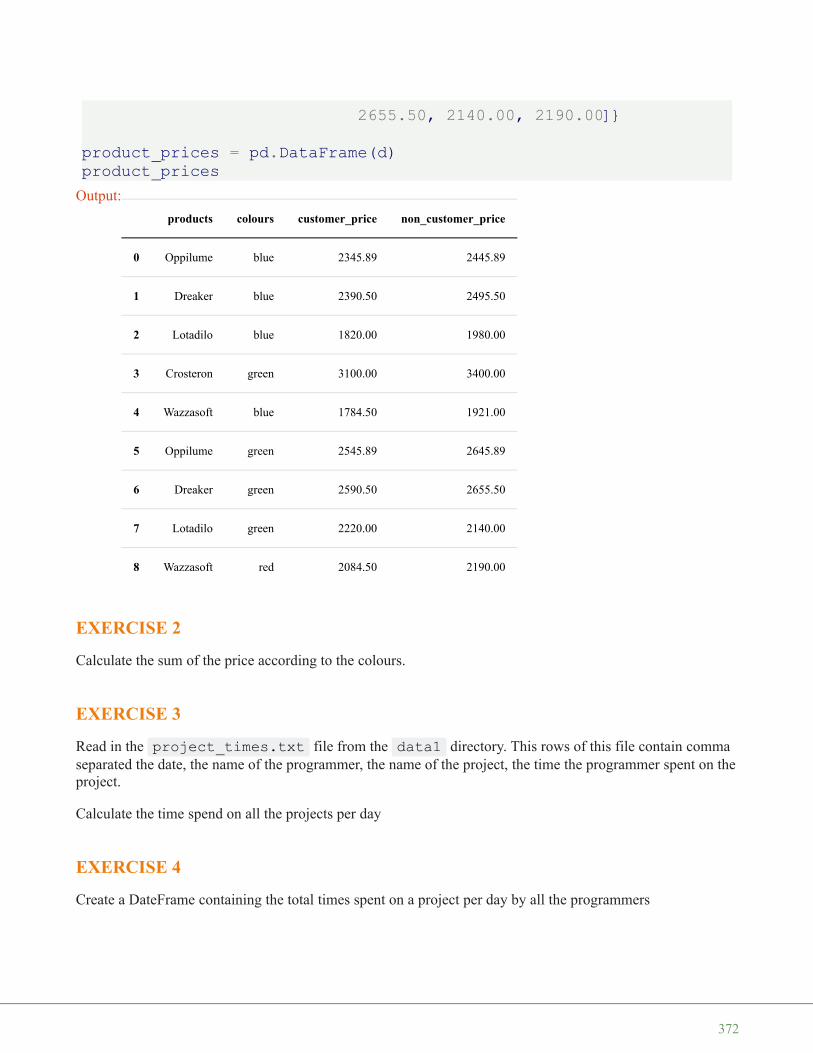
2655.50, 2140.00, 2190.00]}

product_prices = pd.DataFrame(d)product_prices

EXERCISE 2

Calculate the sum of the price according to the colours.

EXERCISE 3

Read in the project_times.txt file from the data1 directory. This rows of this file contain commaseparated the date, the name of the programmer, the name of the project, the time the programmer spent on theproject.

Calculate the time spend on all the projects per day

EXERCISE 4

Create a DateFrame containing the total times spent on a project per day by all the programmers

Output:

products colours customer_price non_customer_price

0 Oppilume blue 2345.89 2445.89

1 Dreaker blue 2390.50 2495.50

2 Lotadilo blue 1820.00 1980.00

3 Crosteron green 3100.00 3400.00

4 Wazzasoft blue 1784.50 1921.00

5 Oppilume green 2545.89 2645.89

6 Dreaker green 2590.50 2655.50

7 Lotadilo green 2220.00 2140.00

8 Wazzasoft red 2084.50 2190.00

372

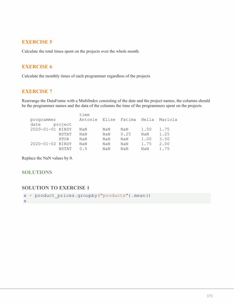
EXERCISE 5

Calculate the total times spent on the projects over the whole month.

EXERCISE 6

Calculate the monthly times of each programmer regardless of the projects

EXERCISE 7

Rearrange the DataFrame with a MultiIndex consisting of the date and the project names, the columns shouldbe the programmer names and the data of the columns the time of the programmers spent on the projects.

timeprogrammer Antonie Elise Fatima Hella Marioladate project2020-01-01 BIRDY NaN NaN NaN 1.50 1.75

NSTAT NaN NaN 0.25 NaN 1.25XTOR NaN NaN NaN 1.00 3.50

2020-01-02 BIRDY NaN NaN NaN 1.75 2.00NSTAT 0.5 NaN NaN NaN 1.75

Replace the NaN values by 0.

SOLUTIONS

SOLUTION TO EXERCISE 1x = product_prices.groupby("products").mean()x

373

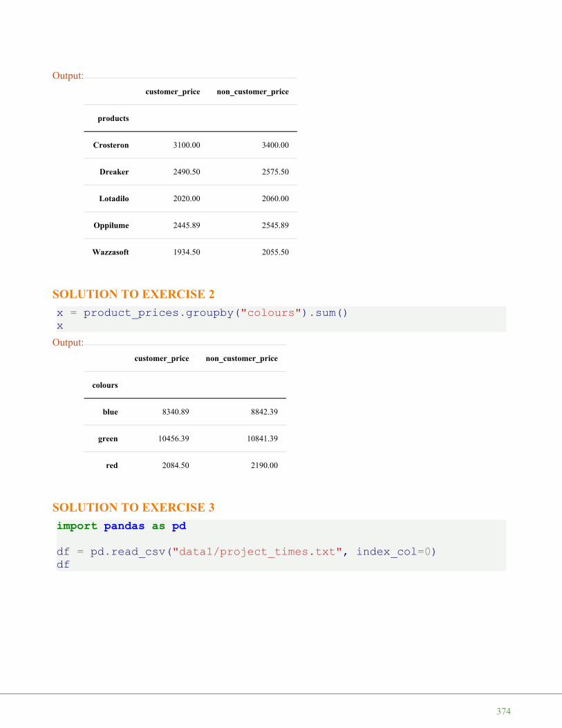
SOLUTION TO EXERCISE 2x = product_prices.groupby("colours").sum()x

SOLUTION TO EXERCISE 3import pandas as pddf = pd.read_csv("data1/project_times.txt", index_col=0)df

Output:

customer_price non_customer_price

products

Crosteron 3100.00 3400.00

Dreaker 2490.50 2575.50

Lotadilo 2020.00 2060.00

Oppilume 2445.89 2545.89

Wazzasoft 1934.50 2055.50

Output:

customer_price non_customer_price

colours

blue 8340.89 8842.39

green 10456.39 10841.39

red 2084.50 2190.00

374

times_per_day = df.groupby(df.index).sum()print(times_per_day[:10])

Output:

programmer project time

date

2020-01-01 Hella XTOR 1.00

2020-01-01 Hella BIRDY 1.50

2020-01-01 Fatima NSTAT 0.25

2020-01-01 Mariola NSTAT 0.50

2020-01-01 Mariola BIRDY 1.75

... ... ... ...

2030-01-30 Antonie XTOR 0.50

2030-01-31 Hella BIRDY 1.25

2030-01-31 Hella BIRDY 1.75

2030-01-31 Mariola BIRDY 1.00

2030-01-31 Hella BIRDY 1.00

17492 rows × 3 columns

timedate2020-01-01 9.252020-01-02 6.002020-01-03 2.502020-01-06 5.752020-01-07 15.002020-01-08 13.252020-01-09 10.252020-01-10 17.002020-01-13 4.752020-01-14 10.00

375

SOLUTION TO EXERCISE 4times_per_day_project = df.groupby([df.index, 'project']).sum()print(times_per_day_project[:10])

SOLUTION TO EXERCISE 5df.groupby(['project']).sum()

SOLUTION TO EXERCISE 6df.groupby(['programmer']).sum()

timedate project2020-01-01 BIRDY 3.25

NSTAT 1.50XTOR 4.50

2020-01-02 BIRDY 3.75NSTAT 2.25

2020-01-03 BIRDY 1.00NSTAT 0.25XTOR 1.25

2020-01-06 BIRDY 2.75NSTAT 0.75

Output:

time

project

BIRDY 9605.75

NSTAT 8707.75

XTOR 6427.50

376

SOLUTION TO EXERCISE 7x = df.groupby([df.index, 'project', 'programmer']).sum()

x = x.unstack()x

Output:

time

programmer

Antonie 1511.25

Elise 80.00

Fatima 593.00

Hella 10642.00

Mariola 11914.75

377

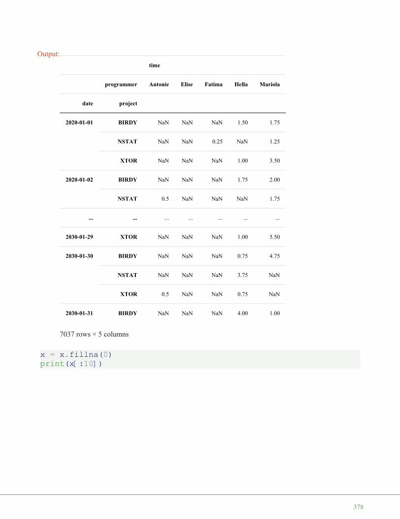
x = x.fillna(0)print(x[:10])

Output:

time

programmer Antonie Elise Fatima Hella Mariola

date project

2020-01-01 BIRDY NaN NaN NaN 1.50 1.75

NSTAT NaN NaN 0.25 NaN 1.25

XTOR NaN NaN NaN 1.00 3.50

2020-01-02 BIRDY NaN NaN NaN 1.75 2.00

NSTAT 0.5 NaN NaN NaN 1.75

... ... ... ... ... ... ...

2030-01-29 XTOR NaN NaN NaN 1.00 5.50

2030-01-30 BIRDY NaN NaN NaN 0.75 4.75

NSTAT NaN NaN NaN 3.75 NaN

XTOR 0.5 NaN NaN 0.75 NaN

2030-01-31 BIRDY NaN NaN NaN 4.00 1.00

7037 rows × 5 columns

378

timeprogrammer Antonie Elise Fatima Hella Marioladate project2020-01-01 BIRDY 0.00 0.0 0.00 1.50 1.75

NSTAT 0.00 0.0 0.25 0.00 1.25XTOR 0.00 0.0 0.00 1.00 3.50

2020-01-02 BIRDY 0.00 0.0 0.00 1.75 2.00NSTAT 0.50 0.0 0.00 0.00 1.75

2020-01-03 BIRDY 0.00 0.0 1.00 0.00 0.00NSTAT 0.25 0.0 0.00 0.00 0.00XTOR 0.00 0.0 0.00 0.50 0.75

2020-01-06 BIRDY 0.00 0.0 0.00 2.50 0.25NSTAT 0.00 0.0 0.00 0.00 0.75

379

R E A D I N G A N D W R I T I N G D A T A

All the powerful data structures like the Series and theDataFrames would avail to nothing, if the Pandas modulewouldn't provide powerful functionalities for reading inand writing out data. It is not only a matter of having afunctions for interacting with files. To be useful to datascientists it also needs functions which support the mostimportant data formats like

• Delimiter-separated files, like e.g. csv• Microsoft Excel files• HTML• XML• JSON

DELIMITER-SEPARATED VALUES

Most people take csv files as a synonym for delimter-separated values files. They leave the fact out of accountthat csv is an acronym for "comma separated values",which is not the case in many situations. Pandas also uses"csv" and contexts, in which "dsv" would be moreappropriate.

Delimiter-separated values (DSV) are defined and storedtwo-dimensional arrays (for example strings) of data byseparating the values in each row with delimiter characters defined for this purpose. This way of implementingdata is often used in combination of spreadsheet programs, which can read in and write out data as DSV. Theyare also used as a general data exchange format.

We call a text file a "delimited text file" if it contains text in DSV format.

For example, the file dollar_euro.txt is a delimited text file and uses tabs (\t) as delimiters.

READING CSV AND DSV FILES

Pandas offers two ways to read in CSV or DSV files to be precise:

• DataFrame.from_csv• read_csv

There is no big difference between those two functions, e.g. they have different default values in some casesand read_csv has more paramters. We will focus on read_csv, because DataFrame.from_csv is kept insidePandas for reasons of backwards compatibility.

380

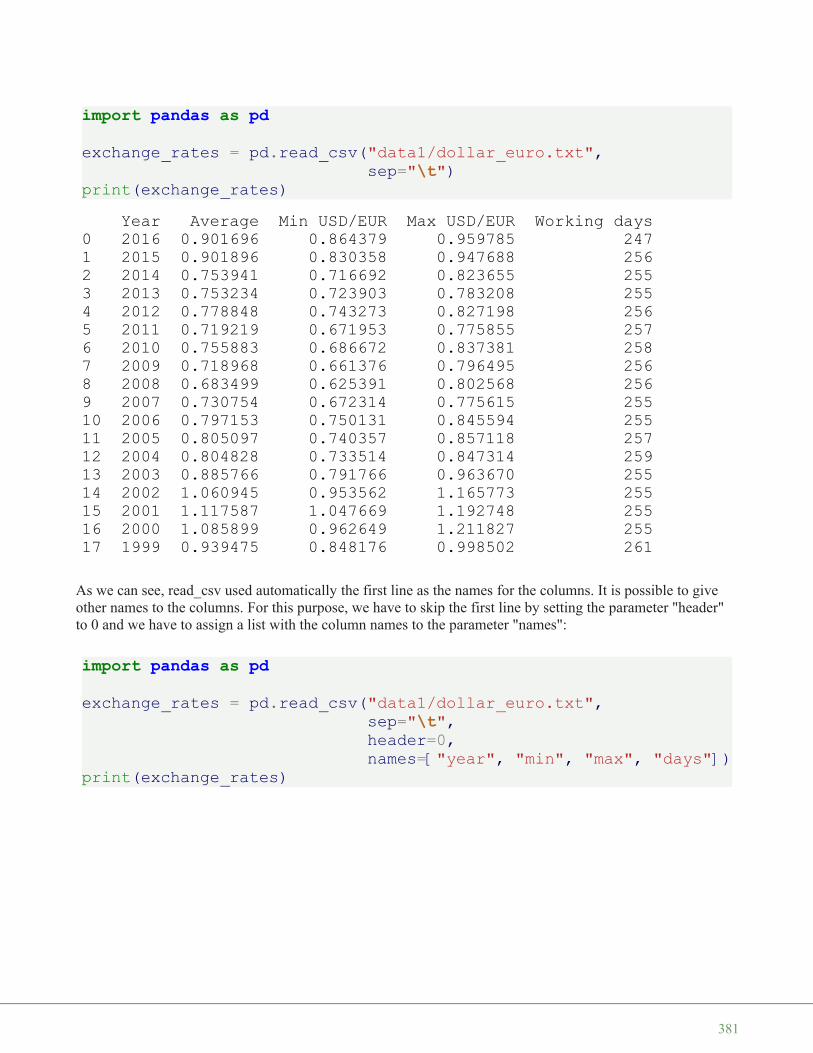
import pandas as pdexchange_rates = pd.read_csv("data1/dollar_euro.txt",

sep="\t")print(exchange_rates)

As we can see, read_csv used automatically the first line as the names for the columns. It is possible to giveother names to the columns. For this purpose, we have to skip the first line by setting the parameter "header"to 0 and we have to assign a list with the column names to the parameter "names":

import pandas as pdexchange_rates = pd.read_csv("data1/dollar_euro.txt",

sep="\t",header=0,names=["year", "min", "max", "days"])

print(exchange_rates)

Year Average Min USD/EUR Max USD/EUR Working days0 2016 0.901696 0.864379 0.959785 2471 2015 0.901896 0.830358 0.947688 2562 2014 0.753941 0.716692 0.823655 2553 2013 0.753234 0.723903 0.783208 2554 2012 0.778848 0.743273 0.827198 2565 2011 0.719219 0.671953 0.775855 2576 2010 0.755883 0.686672 0.837381 2587 2009 0.718968 0.661376 0.796495 2568 2008 0.683499 0.625391 0.802568 2569 2007 0.730754 0.672314 0.775615 25510 2006 0.797153 0.750131 0.845594 25511 2005 0.805097 0.740357 0.857118 25712 2004 0.804828 0.733514 0.847314 25913 2003 0.885766 0.791766 0.963670 25514 2002 1.060945 0.953562 1.165773 25515 2001 1.117587 1.047669 1.192748 25516 2000 1.085899 0.962649 1.211827 25517 1999 0.939475 0.848176 0.998502 261

381

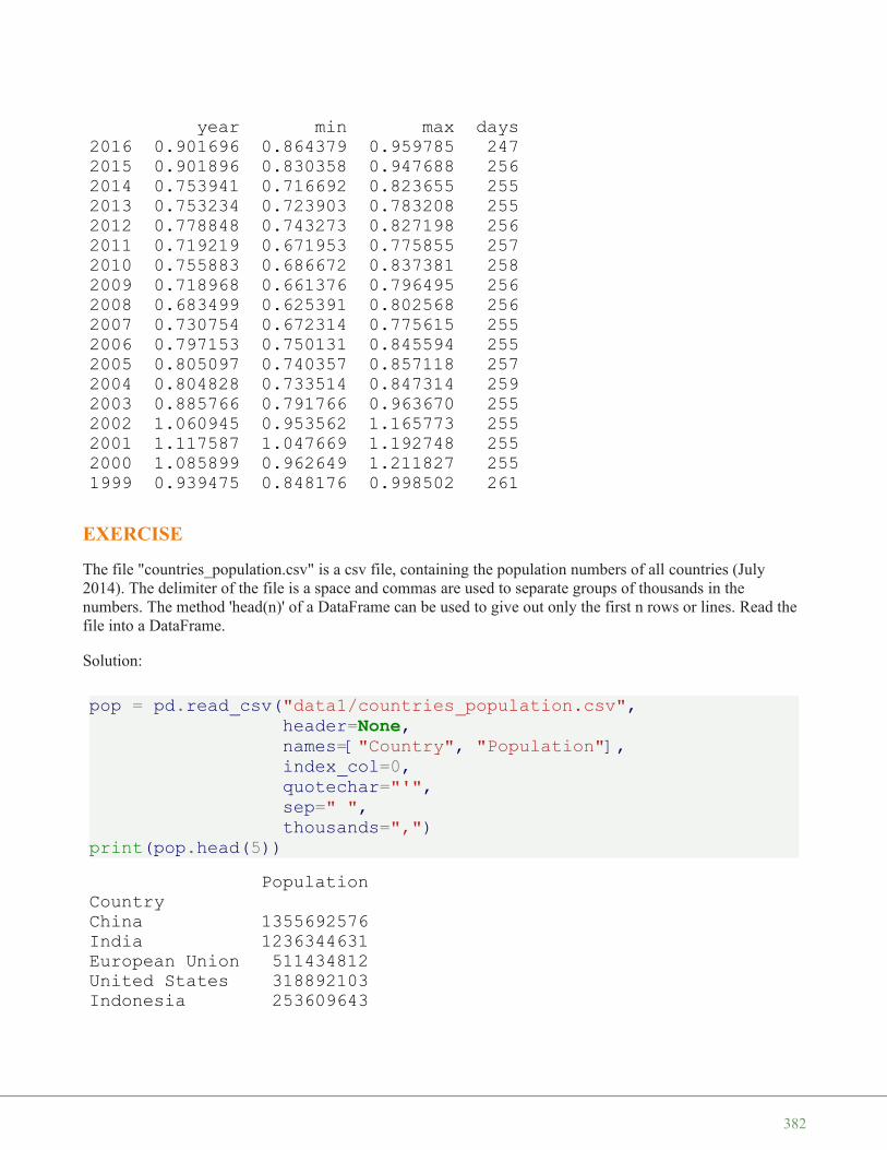
EXERCISE

The file "countries_population.csv" is a csv file, containing the population numbers of all countries (July2014). The delimiter of the file is a space and commas are used to separate groups of thousands in thenumbers. The method 'head(n)' of a DataFrame can be used to give out only the first n rows or lines. Read thefile into a DataFrame.

Solution:

pop = pd.read_csv("data1/countries_population.csv",header=None,names=["Country", "Population"],index_col=0,quotechar="'",sep=" ",thousands=",")

print(pop.head(5))

year min max days2016 0.901696 0.864379 0.959785 2472015 0.901896 0.830358 0.947688 2562014 0.753941 0.716692 0.823655 2552013 0.753234 0.723903 0.783208 2552012 0.778848 0.743273 0.827198 2562011 0.719219 0.671953 0.775855 2572010 0.755883 0.686672 0.837381 2582009 0.718968 0.661376 0.796495 2562008 0.683499 0.625391 0.802568 2562007 0.730754 0.672314 0.775615 2552006 0.797153 0.750131 0.845594 2552005 0.805097 0.740357 0.857118 2572004 0.804828 0.733514 0.847314 2592003 0.885766 0.791766 0.963670 2552002 1.060945 0.953562 1.165773 2552001 1.117587 1.047669 1.192748 2552000 1.085899 0.962649 1.211827 2551999 0.939475 0.848176 0.998502 261

PopulationCountryChina 1355692576India 1236344631European Union 511434812United States 318892103Indonesia 253609643

382

WRITING CSV FILES

We can create csv (or dsv) files with the method "to_csv". Before we do this, we will prepare some data tooutput, which we will write to a file. We have two csv files with population data for various countries.countries_male_population.csv contains the figures of the male populations andcountries_female_population.csv correspondingly the numbers for the female populations. We will create anew csv file with the sum:

column_names = ["Country"] + list(range(2002, 2013))male_pop = pd.read_csv("data1/countries_male_population.csv",

header=None,index_col=0,names=column_names)

female_pop = pd.read_csv("data1/countries_female_population.csv",header=None,index_col=0,names=column_names)

population = male_pop + female_poppopulation

383

Output:

2002 2003 2004 2005 2006 2007 2008 2009

Country

Australia 19640979.0 19872646 20091504 20339759 20605488 21015042 21431781 21874920

Austria 8139310.0 8067289 8140122 8206524 8265925 8298923 8331930 8355260

Belgium 10309725.0 10355844 10396421 10445852 10511382 10584534 10666866 10753080

Canada NaN 31361611 31372587 31989454 32299496 32649482 32927372 33327337

CzechRepublic 10269726.0 10203269 10211455 10220577 10251079 10287189 10381130 10467542

Denmark 5368354.0 5383507 5397640 5411405 5427459 5447084 5475791 5511451

Finland 5194901.0 5206295 5219732 5236611 5255580 5276955 5300484 5326314

France 59337731.0 59630121 59900680 62518571 62998773 63392140 63753140 64366962

Germany 82440309.0 82536680 82531671 82500849 82437995 82314906 82217837 82002356

Greece 10988000.0 11006377 11040650 11082751 11125179 11171740 11213785 11260402

Hungary 10174853.0 10142362 10116742 10097549 10076581 10066158 10045401 10030975

Iceland 286575.0 288471 290570 293577 299891 307672 315459 319368

Ireland 3882683.0 3963636 4027732 4109173 4209019 4239848 4401335 4450030

Italy 56993742.0 57321070 57888245 58462375 58751711 59131287 59619290 60045068

Japan 127291000.0 127435000 127620000 127687000 127767994 127770000 127771000 127692000

Korea 47639618.0 47925318 48082163 48138077 48297184 48456369 48606787 48746693

Luxembourg 444050.0 448300 451600 455000 469086 476187 483799 493500

Mexico 101826249.0 103039964 104213503 103001871 103946866 104874282 105790725 106682518

Netherlands 16105285.0 16192572 16258032 16305526 16334210 16357992 16405399 16485787

384

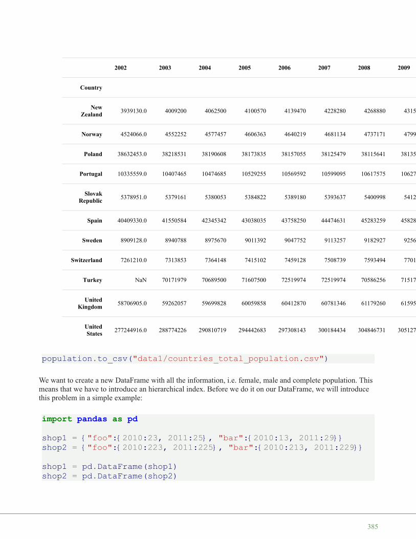
population.to_csv("data1/countries_total_population.csv")

We want to create a new DataFrame with all the information, i.e. female, male and complete population. Thismeans that we have to introduce an hierarchical index. Before we do it on our DataFrame, we will introducethis problem in a simple example:

import pandas as pdshop1 = {"foo":{2010:23, 2011:25}, "bar":{2010:13, 2011:29}}shop2 = {"foo":{2010:223, 2011:225}, "bar":{2010:213, 2011:229}}

shop1 = pd.DataFrame(shop1)shop2 = pd.DataFrame(shop2)

2002 2003 2004 2005 2006 2007 2008 2009

Country

NewZealand 3939130.0 4009200 4062500 4100570 4139470 4228280 4268880 4315840

Norway 4524066.0 4552252 4577457 4606363 4640219 4681134 4737171 4799252

Poland 38632453.0 38218531 38190608 38173835 38157055 38125479 38115641 38135876

Portugal 10335559.0 10407465 10474685 10529255 10569592 10599095 10617575 10627250

SlovakRepublic 5378951.0 5379161 5380053 5384822 5389180 5393637 5400998 5412254

Spain 40409330.0 41550584 42345342 43038035 43758250 44474631 45283259 45828172

Sweden 8909128.0 8940788 8975670 9011392 9047752 9113257 9182927 9256347

Switzerland 7261210.0 7313853 7364148 7415102 7459128 7508739 7593494 7701856

Turkey NaN 70171979 70689500 71607500 72519974 72519974 70586256 71517100

UnitedKingdom 58706905.0 59262057 59699828 60059858 60412870 60781346 61179260 61595094

UnitedStates 277244916.0 288774226 290810719 294442683 297308143 300184434 304846731 305127551

385

both_shops = shop1 + shop2print("Sales of shop1:\n", shop1)print("\nSales of both shops\n", both_shops)

shops = pd.concat([shop1, shop2], keys=["one", "two"])shops

We want to swap the hierarchical indices. For this we will use 'swaplevel':

shops.swaplevel()shops.sort_index(inplace=True)shops

Sales of shop1:foo bar

2010 23 132011 25 29

Sales of both shopsfoo bar

2010 246 2262011 250 258

Output:

foo bar

one 2010 23 13

2011 25 29

two 2010 223 213

2011 225 229

386

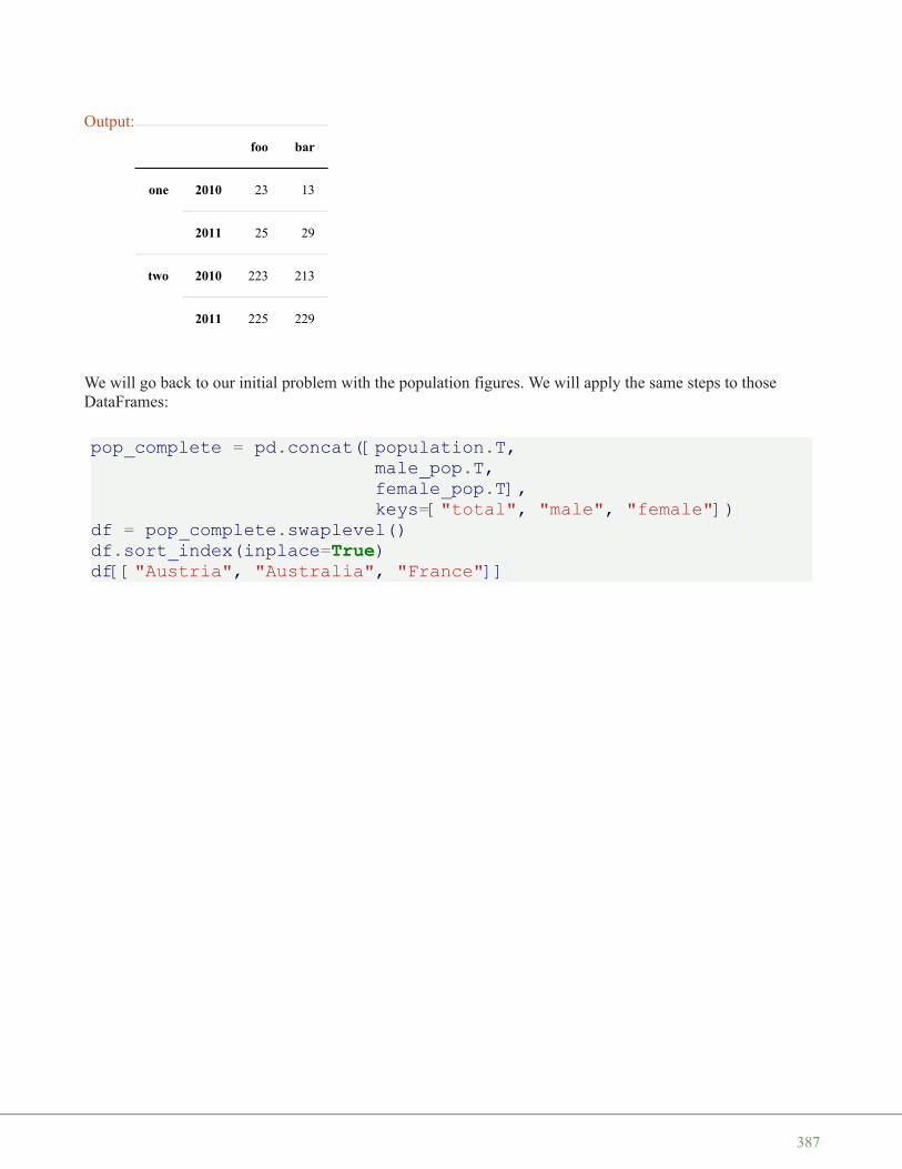
We will go back to our initial problem with the population figures. We will apply the same steps to thoseDataFrames:

pop_complete = pd.concat([population.T,male_pop.T,female_pop.T],keys=["total", "male", "female"])

df = pop_complete.swaplevel()df.sort_index(inplace=True)df[["Austria", "Australia", "France"]]

Output:

foo bar

one 2010 23 13

2011 25 29

two 2010 223 213

2011 225 229

387

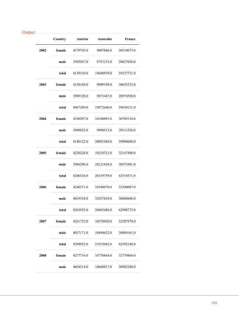
Output:

Country Austria Australia France

2002 female 4179743.0 9887846.0 30510073.0

male 3959567.0 9753133.0 28827658.0

total 8139310.0 19640979.0 59337731.0

2003 female 4158169.0 9999199.0 30655533.0

male 3909120.0 9873447.0 28974588.0

total 8067289.0 19872646.0 59630121.0

2004 female 4190297.0 10100991.0 30789154.0

male 3949825.0 9990513.0 29111526.0

total 8140122.0 20091504.0 59900680.0

2005 female 4220228.0 10218321.0 32147490.0

male 3986296.0 10121438.0 30371081.0

total 8206524.0 20339759.0 62518571.0

2006 female 4246571.0 10348070.0 32390087.0

male 4019354.0 10257418.0 30608686.0

total 8265925.0 20605488.0 62998773.0

2007 female 4261752.0 10570420.0 32587979.0

male 4037171.0 10444622.0 30804161.0

total 8298923.0 21015042.0 63392140.0

2008 female 4277716.0 10770864.0 32770860.0

male 4054214.0 10660917.0 30982280.0

388

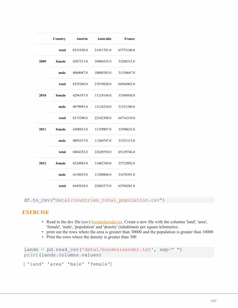
df.to_csv("data1/countries_total_population.csv")

EXERCISE

• Read in the dsv file (csv) bundeslaender.txt. Create a new file with the columns 'land', 'area','female', 'male', 'population' and 'density' (inhabitants per square kilometres.

• print out the rows where the area is greater than 30000 and the population is greater than 10000• Print the rows where the density is greater than 300

lands = pd.read_csv('data1/bundeslaender.txt', sep=" ")print(lands.columns.values)

Country Austria Australia France

total 8331930.0 21431781.0 63753140.0

2009 female 4287213.0 10986535.0 33208315.0

male 4068047.0 10888385.0 31158647.0

total 8355260.0 21874920.0 64366962.0

2010 female 4296197.0 11218144.0 33384930.0

male 4079093.0 11124254.0 31331380.0

total 8375290.0 22342398.0 64716310.0

2011 female 4308915.0 11359807.0 33598633.0

male 4095337.0 11260747.0 31531113.0

total 8404252.0 22620554.0 65129746.0

2012 female 4324983.0 11402769.0 33723892.0

male 4118035.0 11280804.0 31670391.0

total 8443018.0 22683573.0 65394283.0

['land' 'area' 'male' 'female']

389

# swap the columns of our DataFrame:lands = lands.reindex(columns=['land', 'area', 'female', 'male'])lands[:2]

lands.insert(loc=len(lands.columns),column='population',value=lands['female'] + lands['male'])

lands[:3]

lands.insert(loc=len(lands.columns),column='density',value=(lands['population'] * 1000 / lands['area']).ro

und(0))

lands[:4]

Output:

land area female male

0 Baden-Württemberg 35751.65 5465 5271

1 Bayern 70551.57 6366 6103

Output:

land area female male population

0 Baden-Württemberg 35751.65 5465 5271 10736

1 Bayern 70551.57 6366 6103 12469

2 Berlin 891.85 1736 1660 3396

Output:

land area female male population density

0 Baden-Württemberg 35751.65 5465 5271 10736 300.0

1 Bayern 70551.57 6366 6103 12469 177.0

2 Berlin 891.85 1736 1660 3396 3808.0

3 Brandenburg 29478.61 1293 1267 2560 87.0

390

print(lands.loc[(lands.area>30000) & (lands.population>10000)])

READING AND WRITING EXCEL FILES

It is also possible to read and write Microsoft Excel files. The Pandas functionalities to read and write Excelfiles use the modules 'xlrd' and 'openpyxl'. These modules are not automatically installed by Pandas, so youmay have to install them manually!

We will use a simple Excel document to demonstrate the reading capabilities of Pandas. The documentsales.xls contains two sheets, one called 'week1' and the other one 'week2'.An Excel file can be read in with the Pandas function "read_excel". This is demonstrated in the followingexample Python code:

excel_file = pd.ExcelFile("data1/sales.xls")

sheet = pd.read_excel(excel_file)sheet

The document "sales.xls" contains two sheets, but we only have been able to read in the first one with"read_excel". A complete Excel document, which can consist of an arbitrary number of sheets, can becompletely read in like this:

land area female male population density0 Baden-Württemberg 35751.65 5465 5271 10736 300.01 Bayern 70551.57 6366 6103 12469 177.09 Nordrhein-Westfalen 34085.29 9261 8797 18058 530.0

Output:

Weekday Sales

0 Monday 123432.980000

1 Tuesday 122198.650200

2 Wednesday 134418.515220

3 Thursday 131730.144916

4 Friday 128173.431003

391

docu = {}for sheet_name in excel_file.sheet_names:

docu[sheet_name] = excel_file.parse(sheet_name)

for sheet_name in docu:print("\n" + sheet_name + ":\n", docu[sheet_name])

We will calculate now the avarage sales numbers of the two weeks:

average = docu["week1"].copy()average["Sales"] = (docu["week1"]["Sales"] + docu["week2"]["Sales"]) / 2print(average)

We will save the DataFrame 'average' in a new document with 'week1' and 'week2' as additional sheets as well:

writer = pd.ExcelWriter('data1/sales_average.xlsx')document['week1'].to_excel(writer,'week1')document['week2'].to_excel(writer,'week2')average.to_excel(writer,'average')writer.save()writer.close()

week1:Weekday Sales

0 Monday 123432.9800001 Tuesday 122198.6502002 Wednesday 134418.5152203 Thursday 131730.1449164 Friday 128173.431003

week2:Weekday Sales

0 Monday 223277.9800001 Tuesday 234441.8790002 Wednesday 246163.9729503 Thursday 241240.6934914 Friday 230143.621590

Weekday Sales0 Monday 173355.4800001 Tuesday 178320.2646002 Wednesday 190291.2440853 Thursday 186485.4192034 Friday 179158.526297

392

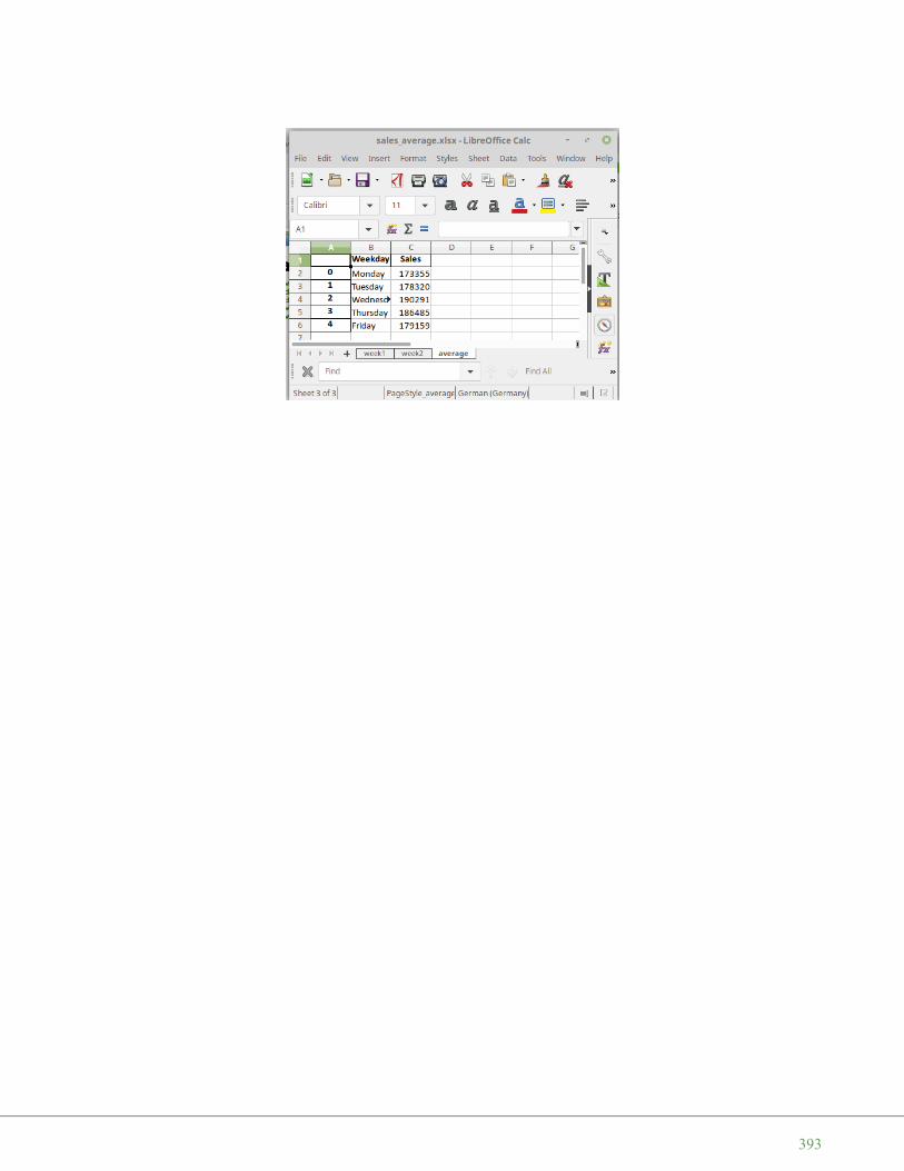
393

D E A L I N G W I T H N A N

INTRODUCTION

NaN was introduced, at least officially, bythe IEEE Standard for Floating-PointArithmetic (IEEE 754). It is a technicalstandard for floating-point computationestablished in 1985 - many years beforePython was invented, and even a longertime befor Pandas was created - by theInstitute of Electrical and ElectronicsEngineers (IEEE). It was introduced tosolve problems found in many floatingpoint implementations that made themdifficult to use reliably and portably.

This standard added NaN to the arithmeticformats: "arithmetic formats: sets ofbinary and decimal floating-point data,which consist of finite numbers (includingsigned zeros and subnormal numbers),infinities, and special 'not a number' values (NaNs)"

'NAN' IN PYTHON

Python knows NaN values as well. We can create it with "float":

n1 = float("nan")n2 = float("Nan")n3 = float("NaN")n4 = float("NAN")print(n1, n2, n3, n4)

"nan" is also part of the math module since Python 3.5:

nan nan nan nan

394

import mathn1 = math.nanprint(n1)print(math.isnan(n1))

Warning: Do not perform comparison between "NaN" values or "Nan" values and regular numbers. A simpleor simplified reasoning is this: Two things are "not a number", so they can be anything but most probably notthe same. Above all there is no way of ordering NaNs:

print(n1 == n2)print(n1 == 0)print(n1 == 100)print(n2 < 0)

NAN IN PANDAS

EXAMPLE WITHOUT NANS

Before we will work with NaN data, we will process a file without any NaN values. The data filetemperatures.csv contains the temperature data of six sensors taken every 15 minuts between 6:00 to 19.15o'clock.

Reading in the data file can be done with the read_csv function:

import pandas as pddf = pd.read_csv("data1/temperatures.csv",

sep=";",decimal=",")

df.loc[:3]

nanTrue

FalseFalseFalseFalse

395

We want to calculate the avarage temperatures per measuring point over all the sensors. We can use theDataFrame method 'mean'. If we use 'mean' without parameters it will sum up the sensor columns, which isn'twhat we want, but it may be interesting as well:

df.mean()

average_temp_series = df.mean(axis=1)print(average_temp_series[:8])

sensors = df.columns.values[1:]# all columns except the time column will be removed:df = df.drop(sensors, axis=1)print(df[:5])

Output:

time sensor1 sensor2 sensor3 sensor4 sensor5 sensor6

0 06:00:00 14.3 13.7 14.2 14.3 13.5 13.6

1 06:15:00 14.5 14.5 14.0 15.0 14.5 14.7

2 06:30:00 14.6 15.1 14.8 15.3 14.0 14.2

3 06:45:00 14.8 14.5 15.6 15.2 14.7 14.6

Output: sensor1 19.775926sensor2 19.757407sensor3 19.840741sensor4 20.187037sensor5 19.181481sensor6 19.437037dtype: float64

0 13.9333331 14.5333332 14.6666673 14.9000004 15.0833335 15.1166676 15.2833337 15.116667dtype: float64

396

We will assign now the average temperature values as a new column 'temperature':

# best practice:df = df.assign(temperature=average_temp_series) # inplace optionnot available

# alternatively:#df.loc[:,"temperature"] = average_temp_series

df[:3]

EXAMPLE WITH NANS

We will use now a data file similar to the previous temperature csv, but this time we will have to cope withNaN data, when the sensors malfunctioned.

We will create a temperature DataFrame, in which some data is not defined, i.e. NaN.

We will use and change the data from the the temperatures.csv file:

import pandas as pdtemp_df = pd.read_csv("data1/temperatures.csv",

sep=";",index_col=0,decimal=",")

temp_df[:8]

time0 06:00:001 06:15:002 06:30:003 06:45:004 07:00:00

Output:

time temperature

0 06:00:00 13.933333

1 06:15:00 14.533333

2 06:30:00 14.666667

397

We will randomly assign some NaN values into the data frame. For this purpose, we will use the wheremethod from DataFrame. If we apply where to a DataFrame object df, i.e. df.where(cond, other_df), it willreturn an object of same shape as df and whose corresponding entries are from df where the correspondingelement of cond is True and otherwise are taken from other_df.

Before we continue with our task, we will demonstrate the way of working of where with some simpleexamples:

s = pd.Series(range(5)) s.where(s > 0)

import numpy as npA = np.random.randint(1, 30, (4, 2))

df = pd.DataFrame(A, columns=['Foo', 'Bar'])m = df % 2 == 0df.where(m, -df, inplace=True)df

Output:

sensor1 sensor2 sensor3 sensor4 sensor5 sensor6

time

06:00:00 14.3 13.7 14.2 14.3 13.5 13.6

06:15:00 14.5 14.5 14.0 15.0 14.5 14.7

06:30:00 14.6 15.1 14.8 15.3 14.0 14.2

06:45:00 14.8 14.5 15.6 15.2 14.7 14.6

07:00:00 15.0 14.9 15.7 15.6 14.0 15.3

07:15:00 15.2 15.2 14.6 15.3 15.5 14.9

07:30:00 15.4 15.3 15.6 15.6 14.7 15.1

07:45:00 15.5 14.8 15.4 15.5 14.6 14.9

398

For our task, we need to create a DataFrame 'nan_df', which consists purely of NaN values and has the sameshape as our temperature DataFrame 'temp_df'. We will use this DataFrame in 'where'. We also need aDataFrame with the conditions "df_bool" as True values. For this purpose we will create a DataFrame withrandom values between 0 and 1 and by applying 'random_df < 0.8' we get the df_bool DataFrame, in whichabout 20 % of the values will be True:

random_df = pd.DataFrame(np.random.random(size=temp_df.shape),columns=temp_df.columns.values,index=temp_df.index)

nan_df = pd.DataFrame(np.nan,columns=temp_df.columns.values,index=temp_df.index)

df_bool = random_df<0.8

df_bool[:5]

Output:

Foo Bar

0 18 -5

1 22 -7

2 14 -3

3 16 -23

Output:

sensor1 sensor2 sensor3 sensor4 sensor5 sensor6

time

06:00:00 True True True True True True

06:15:00 True True True False True True

06:30:00 True True True True True False

06:45:00 True True True True False True

07:00:00 True True True True True True

399

Finally, we have everything toghether to create our DataFrame with distrubed measurements:

disturbed_data = temp_df.where(df_bool, nan_df)

disturbed_data.to_csv("data1/temperatures_with_NaN.csv")disturbed_data[:10]

USING DROPNA ON THE DATAFRAME

'dropna' is a DataFrame method. If we call this method without arguments, it will return an object where everyrow is ommitted, in which data are missing, i.e. some value is NaN:

df = disturbed_data.dropna()df

Output:

sensor1 sensor2 sensor3 sensor4 sensor5 sensor6

time

06:00:00 14.3 13.7 14.2 14.3 13.5 13.6

06:15:00 14.5 14.5 14.0 NaN 14.5 14.7

06:30:00 14.6 15.1 14.8 15.3 14.0 NaN

06:45:00 14.8 14.5 15.6 15.2 NaN 14.6

07:00:00 15.0 14.9 15.7 15.6 14.0 15.3

07:15:00 NaN 15.2 14.6 15.3 15.5 14.9

07:30:00 15.4 15.3 15.6 15.6 14.7 NaN

07:45:00 15.5 14.8 15.4 15.5 14.6 14.9

08:00:00 15.7 15.6 15.9 16.2 15.4 15.4

08:15:00 15.9 15.8 15.9 NaN 16.0 16.2

400

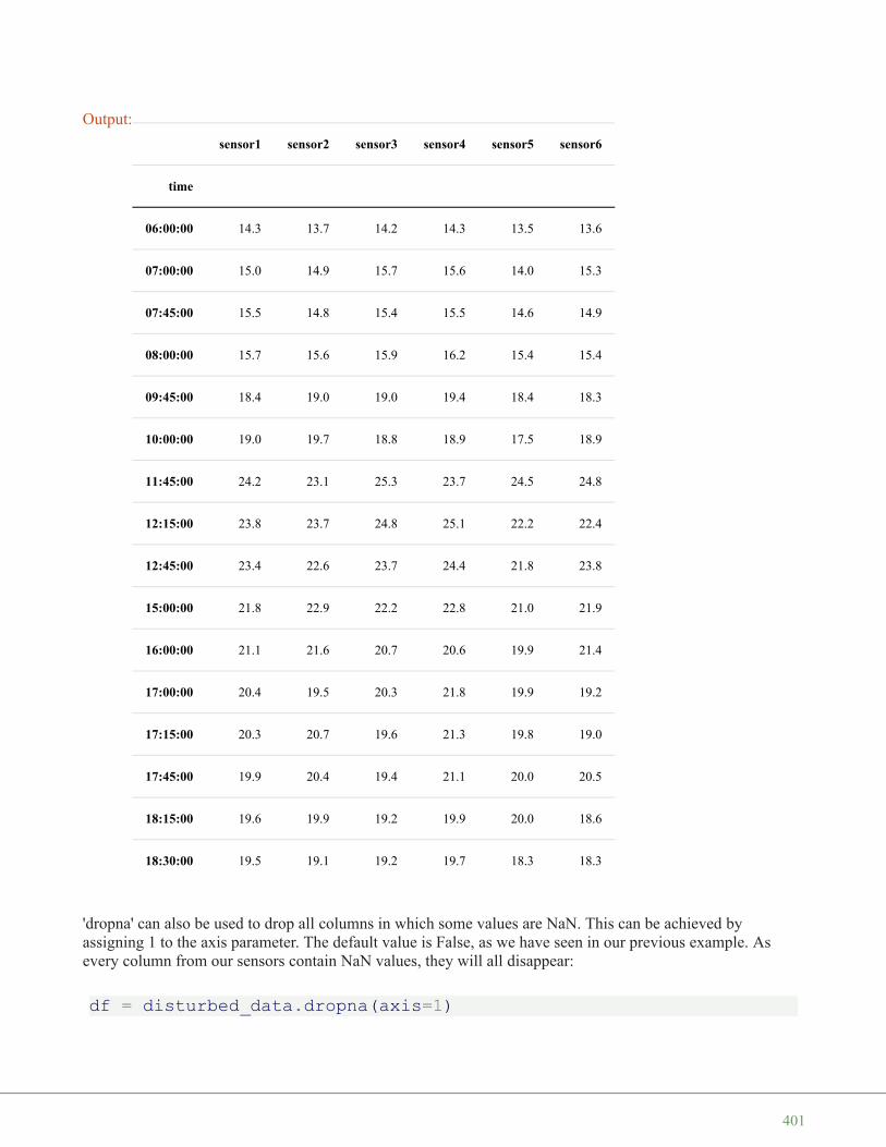
'dropna' can also be used to drop all columns in which some values are NaN. This can be achieved byassigning 1 to the axis parameter. The default value is False, as we have seen in our previous example. Asevery column from our sensors contain NaN values, they will all disappear:

df = disturbed_data.dropna(axis=1)

Output:

sensor1 sensor2 sensor3 sensor4 sensor5 sensor6

time

06:00:00 14.3 13.7 14.2 14.3 13.5 13.6

07:00:00 15.0 14.9 15.7 15.6 14.0 15.3

07:45:00 15.5 14.8 15.4 15.5 14.6 14.9

08:00:00 15.7 15.6 15.9 16.2 15.4 15.4

09:45:00 18.4 19.0 19.0 19.4 18.4 18.3

10:00:00 19.0 19.7 18.8 18.9 17.5 18.9

11:45:00 24.2 23.1 25.3 23.7 24.5 24.8

12:15:00 23.8 23.7 24.8 25.1 22.2 22.4

12:45:00 23.4 22.6 23.7 24.4 21.8 23.8

15:00:00 21.8 22.9 22.2 22.8 21.0 21.9

16:00:00 21.1 21.6 20.7 20.6 19.9 21.4

17:00:00 20.4 19.5 20.3 21.8 19.9 19.2

17:15:00 20.3 20.7 19.6 21.3 19.8 19.0

17:45:00 19.9 20.4 19.4 21.1 20.0 20.5

18:15:00 19.6 19.9 19.2 19.9 20.0 18.6

18:30:00 19.5 19.1 19.2 19.7 18.3 18.3

401

df[:5]

Let us change our task: We only want to get rid of all the rows, which contain more than one NaN value. Theparameter 'thresh' is ideal for this task. It can be set to the minimum number. 'thresh' is set to an integer value,which defines the minimum number of non-NaN values. We have six temperature values in every row. Setting'thresh' to 5 makes sure that we will have at least 5 valid floats in every remaining row:

cleansed_df = disturbed_data.dropna(thresh=5, axis=0)cleansed_df[:7]

Output:

time

06:00:00

06:15:00

06:30:00

06:45:00

07:00:00

Output:

sensor1 sensor2 sensor3 sensor4 sensor5 sensor6

time

06:00:00 14.3 13.7 14.2 14.3 13.5 13.6

06:15:00 14.5 14.5 14.0 NaN 14.5 14.7

06:30:00 14.6 15.1 14.8 15.3 14.0 NaN

06:45:00 14.8 14.5 15.6 15.2 NaN 14.6

07:00:00 15.0 14.9 15.7 15.6 14.0 15.3

07:15:00 NaN 15.2 14.6 15.3 15.5 14.9

07:30:00 15.4 15.3 15.6 15.6 14.7 NaN

402

Now we will calculate the mean values again, but this time on the DataFrame 'cleansed_df', i.e. where we havetaken out all the rows, where more than one NaN value occurred.

average_temp_series = cleansed_df.mean(axis=1)sensors = cleansed_df.columns.valuesdf = cleansed_df.drop(sensors, axis=1)

# best practice:df = df.assign(temperature=average_temp_series) # inplace optionnot availabledf[:6]

Output:

temperature

time

06:00:00 13.933333

06:15:00 14.440000

06:30:00 14.760000

06:45:00 14.940000

07:00:00 15.083333

07:15:00 15.100000

403

B I N N I N G I N P Y T H O N A N D P A N D A S

INTRODUCTION

Data binning, which is also known as bucketing ordiscretization, is a technique used in data processing andstatistics. Binning can be used for example, if there aremore possible data points than observed data points. Anexample is to bin the body heights of people into intervalsor categories. Let us assume, we take the heights of 30people. The length values can be between - roughlyguessing - 1.30 metres to 2.50 metres. Theoretically, thereare 120 different cm values possible, but we can have atmost 30 different values from our sample group. One wayto group them could be to put the measured values intobins ranging from 1.30 - 1.50 metres, 1.50 - 1.70 metres,1.70 - 1.90 metres and so on. This means that the originaldata values, will be assigned to a bin into wich they fitaccording to their size. The original values will bereplaced by values representing the corresponding intervals. Binning is a form of quantization.

Bins do not necessarily have to be numerical, they can be categorical values of any kind, like "dogs", "cats","hamsters", and so on.

Binning is also used in image processing, binning. It can be used to reduce the amount of data, by combiningneighboring pixel into single pixels. kxk binning reduces areas of k x k pixels into single pixel.

Pandas provides easy ways to create bins and to bin data. Before we describe these Pandas functionalities, wewill introduce basic Python functions, working on Python lists and tuples.

BINNING IN PYTHON

The following Python function can be used to create bins.

def create_bins(lower_bound, width, quantity):""" create_bins returns an equal-width (distance) partitionin

g.

404

It returns an ascending list of tuples, representing the intervals.

A tuple bins[i], i.e. (bins[i][0], bins[i][1]) with i >0

and i < quantity, satisfies the following conditions:(1) bins[i][0] + width == bins[i][1](2) bins[i-1][0] + width == bins[i][0] and

bins[i-1][1] + width == bins[i][1]"""

bins = []for low in range(lower_bound,

lower_bound + quantity*width + 1, width):bins.append((low, low+width))

return bins

We will create now five bins (quantity=5) with a width of 10 (width=10) starting from 10 (lower_bound=10):

bins = create_bins(lower_bound=10,width=10,quantity=5)

bins

The next function 'find_bin' is called with a list or tuple of bin 'bins', which have to be two-tuples or lists oftwo elements. The function finds the index of the interval, where the value 'value' is contained:

def find_bin(value, bins):""" bins is a list of tuples, like [(0,20), (20, 40), (40, 6

0)],binning returns the smallest index i of bins so thatbin[i][0] <= value < bin[i][1]

"""

for i in range(0, len(bins)):if bins[i][0] <= value < bins[i][1]:

return ireturn -1

from collections import Counter

Output: [(10, 20), (20, 30), (30, 40), (40, 50), (50, 60), (60, 70)]

405

bins = create_bins(lower_bound=50,width=4,quantity=10)

print(bins)

weights_of_persons = [73.4, 69.3, 64.9, 75.6, 74.9, 80.3,78.6, 84.1, 88.9, 90.3, 83.4, 69.3,52.4, 58.3, 67.4, 74.0, 89.3, 63.4]

binned_weights = []

for value in weights_of_persons:bin_index = find_bin(value, bins)print(value, bin_index, bins[bin_index])binned_weights.append(bin_index)

frequencies = Counter(binned_weights)print(frequencies)[(50, 54), (54, 58), (58, 62), (62, 66), (66, 70), (70, 74), (74,78), (78, 82), (82, 86), (86, 90), (90, 94)]73.4 5 (70, 74)69.3 4 (66, 70)64.9 3 (62, 66)75.6 6 (74, 78)74.9 6 (74, 78)80.3 7 (78, 82)78.6 7 (78, 82)84.1 8 (82, 86)88.9 9 (86, 90)90.3 10 (90, 94)83.4 8 (82, 86)69.3 4 (66, 70)52.4 0 (50, 54)58.3 2 (58, 62)67.4 4 (66, 70)74.0 6 (74, 78)89.3 9 (86, 90)63.4 3 (62, 66)Counter({4: 3, 6: 3, 3: 2, 7: 2, 8: 2, 9: 2, 5: 1, 10: 1, 0: 1,2: 1})

406

BINNING WITH PANDAS

The module Pandas of Python provides powerful functionalities for the binning of data. We will demonstratethis by using our previous data.

BINS USED BY PANDAS

We used a list of tuples as bins in our previous example. We have to turn this list into a usable data structurefor the pandas function "cut". This data structure is an IntervalIndex. We can do this withpd.IntervalIndex.from_tuples:

import pandas as pdbins2 = pd.IntervalIndex.from_tuples(bins)

"cut" is the name of the Pandas function, which is needed to bin values into bins. "cut" takes many parametersbut the most important ones are "x" for the actual values und "bins", defining the IntervalIndex. "x" can be any1-dimensional array-like structure, e.g. tuples, lists, nd-arrays and so on:

categorical_object = pd.cut(weights_of_persons, bins2)print(categorical_object)

The result of the Pandas function "cut" is a so-called "Categorical object". Each bin is a category. Thecategories are described in a mathematical notation. "(70, 74]" means that this bins contains values from 70 to74 whereas 70 is not included but 74 is included. Mathematically, this is a half-open interval, i.e. nn interval inwhich one endpoint is included but not the other. Sometimes it is also called an half-closed interval.

We had also defined the bins in our previous chapter as half-open intervals, but the other way round, i.e. leftside closed and the right side open. When we used pd.IntervalIndex.from_tuples, we could have defined the"openness" of this bins by setting the parameter "closed" to one of the values:

• 'left': closed on the left side and open on the right• 'right': (The default) open on the left side and closed on the right• 'both': closed on both sides• 'neither': open on both sides

To have the same behaviour as in our previous chapter, we will set the parameter closed to "left":

bins2 = pd.IntervalIndex.from_tuples(bins, closed="left")

[(70, 74], (66, 70], (62, 66], (74, 78], (74, 78], ..., (58, 62],(66, 70], (70, 74], (86, 90], (62, 66]]Length: 18Categories (11, interval[int64]): [(50, 54] < (54, 58] < (58, 62]< (62, 66] ... (78, 82] < (82, 86] < (86, 90] < (90, 94]]

407

categorical_object = pd.cut(weights_of_persons, bins2)print(categorical_object)

OTHER WAYS TO DEFINE BINS

We used an IntervalIndex as a bin for binning the weight data. The function "cut" can also cope with two otherkinds of bin representations:

• an integer:defining the number of equal-width bins in the range of the values "x". The

range of "x" is extended by .1% on each side to include the minimum

and maximum values of "x".

• sequence of scalars:Defines the bin edges allowing for non-uniform

width. No extension of the range of "x" is done.

categorical_object = pd.cut(weights_of_persons, 18)

print(categorical_object)

sequence_of_scalars = [ x[0] for x in bins]sequence_of_scalars.append(bins[-1][1])print(sequence_of_scalars)categorical_object = pd.cut(weights_of_persons,

sequence_of_scalars,right=False)

print(categorical_object)

[[70, 74), [66, 70), [62, 66), [74, 78), [74, 78), ..., [58, 62),[66, 70), [74, 78), [86, 90), [62, 66)]Length: 18Categories (11, interval[int64]): [[50, 54) < [54, 58) < [58, 62)< [62, 66) ... [78, 82) < [82, 86) < [86, 90) < [90, 94)]

[(71.35, 73.456], (69.244, 71.35], (62.928, 65.033], (75.561, 77.667], (73.456, 75.561], ..., (56.611, 58.717], (67.139, 69.244], (73.456, 75.561], (88.194, 90.3], (62.928, 65.033]]Length: 18Categories (18, interval[float64]): [(52.362, 54.506] < (54.506, 56.611] < (56.611, 58.717] < (58.717, 60.822] ... (81.878, 83.983]< (83.983, 86.089] < (86.089, 88.194] < (88.194, 90.3]]

408

BIN COUNTS AND VALUE COUNTS

The next and most interesting question is now how we can see the actual bin counts. This can be accomplishedwith the function "value_counts":

pd.value_counts(categorical_object)

"categorical_object.codes" provides you with a labelling of the input values into the binning categories:

labels = categorical_object.codeslabels

categories is the IntervalIndex of the categories of the label indices:

categories = categorical_object.categoriescategories

[50, 54, 58, 62, 66, 70, 74, 78, 82, 86, 90, 94][[70, 74), [66, 70), [62, 66), [74, 78), [74, 78), ..., [58, 62),[66, 70), [74, 78), [86, 90), [62, 66)]Length: 18Categories (11, interval[int64]): [[50, 54) < [54, 58) < [58, 62)< [62, 66) ... [78, 82) < [82, 86) < [86, 90) < [90, 94)]

Output: [74, 78) 3[66, 70) 3[86, 90) 2[82, 86) 2[78, 82) 2[62, 66) 2[90, 94) 1[70, 74) 1[58, 62) 1[50, 54) 1[54, 58) 0dtype: int64

Output: array([ 5, 4, 3, 6, 6, 7, 7, 8, 9, 10, 8, 4, 0,2, 4, 6, 9,

3], dtype=int8)

Output: IntervalIndex([[50, 54), [54, 58), [58, 62), [62, 66), [66, 70) ... [74, 78), [78, 82), [82, 86), [86, 90), [90, 94)],

closed='left',dtype='interval[int64]')

409

Correspondence from weights data to bins:

for index in range(len(weights_of_persons)):label_index = labels[index]print(weights_of_persons[index], label_index, categories[labe

l_index] )

categorical_object.categories

NAMING BINS

Let's imagine, we have an University, which confers three levels of Latin honors depending on the grade pointaverage (GPA):

• "summa cum laude" requires a GPA above 3.9• "magna cum laude" if the GPA is above 3.8• "cum laude" if the GPA of 3.6 or above

degrees = ["none", "cum laude", "magna cum laude", "summa cum laude"]student_results = [3.93, 3.24, 2.80, 2.83, 3.91, 3.698, 3.731, 3.2

73.4 5 [70, 74)69.3 4 [66, 70)64.9 3 [62, 66)75.6 6 [74, 78)74.9 6 [74, 78)80.3 7 [78, 82)78.6 7 [78, 82)84.1 8 [82, 86)88.9 9 [86, 90)90.3 10 [90, 94)83.4 8 [82, 86)69.3 4 [66, 70)52.4 0 [50, 54)58.3 2 [58, 62)67.4 4 [66, 70)74.0 6 [74, 78)89.3 9 [86, 90)63.4 3 [62, 66)

Output: IntervalIndex([[50, 54), [54, 58), [58, 62), [62, 66), [66, 70) ... [74, 78), [78, 82), [82, 86), [86, 90), [90, 94)],

closed='left',dtype='interval[int64]')

410

5, 3.24, 3.82, 3.22]

student_results_degrees = pd.cut(student_results, [0, 3.6, 3.8,3.9, 4.0], labels=degrees)pd.value_counts(student_results_degrees)

Let's have a look at the individual degrees of each student:

labels = student_results_degrees.codescategories = student_results_degrees.categories

for index in range(len(student_results)):label_index = labels[index]print(student_results[index], label_index, categories[label_in

dex] )

Output: none 6summa cum laude 2cum laude 2magna cum laude 1dtype: int64

3.93 3 summa cum laude3.24 0 none2.8 0 none2.83 0 none3.91 3 summa cum laude3.698 1 cum laude3.731 1 cum laude3.25 0 none3.24 0 none3.82 2 magna cum laude3.22 0 none

411

P A N D A S T U T O R I A L : M U L T I - L E V E LI N D E X I N G

INTRODUCTION

We learned the basic concepts of Pandasin our previous chapter of our tutorial onPandas. We introduced the data structures

• Series and• DataFrame

We also learned how to create and manipulate the Series and DataFrame objects in numerous Pythonprograms.

Now it is time to learn some further aspects of theses data structures in this chapter of our tutorial.

We will start with advanced indexing possibilities in Pandas.

ADVANCED OR MULTI-LEVEL INDEXING

Advanced or multi-level indexing is available both for Series and for DataFrames. It is a fascinating way ofworking with higher dimensional data, using Pandas data structures. It's an efficient way to store andmanipulate arbitrarily high dimension data in 1-dimensional (Series) and 2-dimensional tabular (DataFrame)structures. In other words, we can work with higher dimensional data in lower dimensions. It's time to presentan example in Python:

import pandas as pdcities = ["Vienna", "Vienna", "Vienna",

"Hamburg", "Hamburg", "Hamburg","Berlin", "Berlin", "Berlin","Zürich", "Zürich", "Zürich"]

index = [cities, ["country", "area", "population","country", "area", "population","country", "area", "population","country", "area", "population"]]

print(index)

data = ["Austria", 414.60, 1805681,

[['Vienna', 'Vienna', 'Vienna', 'Hamburg', 'Hamburg', 'Hamburg','Berlin', 'Berlin', 'Berlin', 'Zürich', 'Zürich', 'Zürich'], ['country', 'area', 'population', 'country', 'area', 'population', 'country', 'area', 'population', 'country', 'area', 'population']]

412

"Germany", 755.00, 1760433,"Germany", 891.85, 3562166,"Switzerland", 87.88, 378884]

city_series = pd.Series(data, index=index)print(city_series)

We can access the data of a city in the following way:

print(city_series["Vienna"])

We can also access the information about the country, area or population of a city. We can do this in two ways:

print(city_series["Vienna"]["area"])

The other way to accomplish it:

print(city_series["Vienna", "area"])

We can also get the content of multiple cities at the same time by using a list of city names as the key:

Vienna country Austriaarea 414.6population 1805681

Hamburg country Germanyarea 755population 1760433

Berlin country Germanyarea 891.85population 3562166

Zürich country Switzerlandarea 87.88population 378884

dtype: object

country Austriaarea 414.6population 1805681dtype: object

414.6

414.6

413

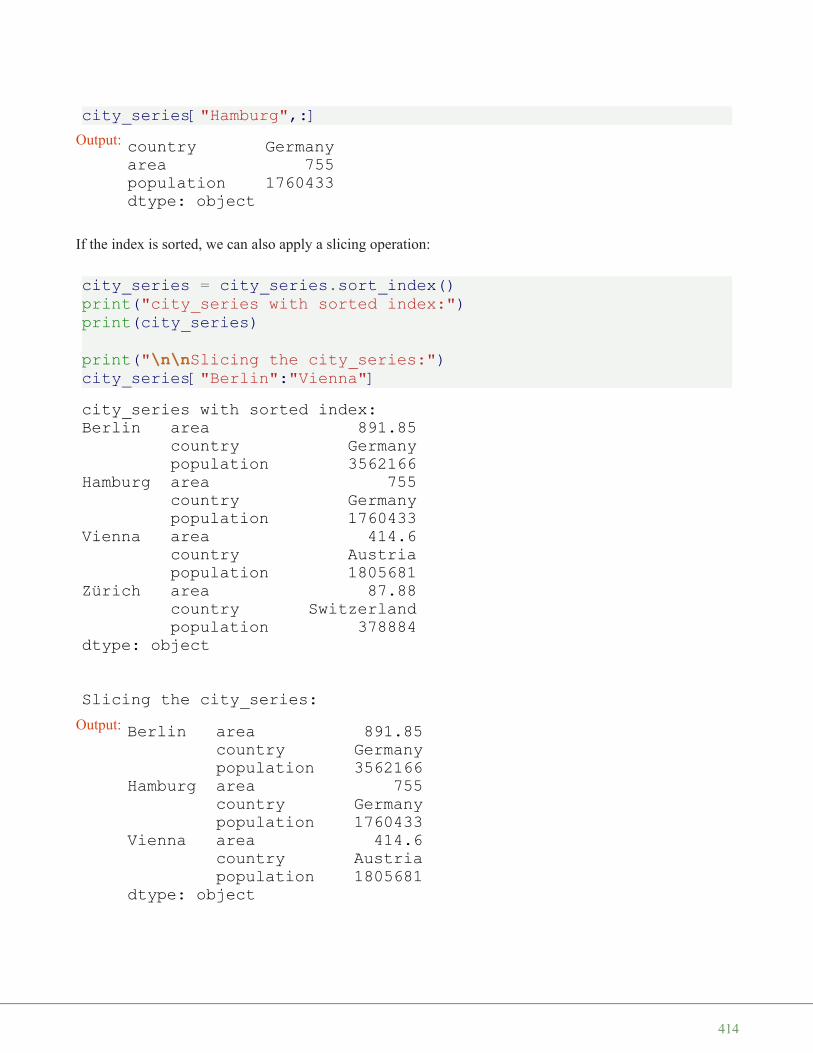
city_series["Hamburg",:]

If the index is sorted, we can also apply a slicing operation:

city_series = city_series.sort_index()print("city_series with sorted index:")print(city_series)

print("\n\nSlicing the city_series:")city_series["Berlin":"Vienna"]

Output: country Germanyarea 755population 1760433dtype: object

city_series with sorted index:Berlin area 891.85

country Germanypopulation 3562166

Hamburg area 755country Germanypopulation 1760433

Vienna area 414.6country Austriapopulation 1805681

Zürich area 87.88country Switzerlandpopulation 378884

dtype: object

Slicing the city_series:Output: Berlin area 891.85

country Germanypopulation 3562166

Hamburg area 755country Germanypopulation 1760433

Vienna area 414.6country Austriapopulation 1805681

dtype: object

414

In the next example, we show that it is possible to access the inner keys as well:

print(city_series[:, "area"])

SWAPPING MULTIINDEX LEVELS

It is possible to swap the levels of a MultiIndex with the method swaplevel:

swaplevel(self, i=-2, j=-1, copy=True)Swap levels i and j in a MultiIndex

Parameters----------i, j : int, string (can be mixed)

Level of index to be swapped. Can pass level name as string.The indexes 'i' and 'j' are optional, and default tothe two innermost levels of the index

Returns-------swapped : Series

city_series = city_series.swaplevel()city_series.sort_index(inplace=True)city_series

Berlin 891.85Hamburg 755Vienna 414.6Zürich 87.88dtype: object

415

Output: area Berlin 891.85Hamburg 755Vienna 414.6Zürich 87.88

country Berlin GermanyHamburg GermanyVienna AustriaZürich Switzerland

population Berlin 3562166Hamburg 1760433Vienna 1805681Zürich 378884

dtype: object

416

D A T A V I S U A L I Z A T I O N W I T H P A N D A S

INTRODUCTIONIt is seldom a good idea topresent your scientific orbusiness data solely in rowsand columns of numbers. Werather use various kinds ofdiagrams to visualize ourdata. This makes thecommunication of informationmore efficiently and easy tograsp. In other words, itmakes complex data moreaccessible and understandable.The numerical data can begraphically encoded with linecharts, bar charts, piecharts, histograms,scatterplots and others.

We have already seen the powerful capabilities of for creating publication-quality plots. Matplotlib is a low-level tool to achieve this goal, because youhave to construe your plots by adding up basic components, like legends, ticklabels, contours and so on.Pandas provides various plotting possibilities, which make like a lot easier.

We will start with an example for a line plot.

LINE PLOT IN PANDAS

SERIESBoth the Pandas Series and DataFrame objects support a plot method.

You can see a simple example of a line plot with for a Series object. We use asimple Python list "data" as the data for the range. The index will be used forthe x values, or the domain.

import pandas as pddata = [100, 120, 140, 180, 200, 210, 214]s = pd.Series(data, index=range(len(data)))

s.plot()

417

It is possible to suppress the usage of the index by setting the keywordparameter "use_index" to False. In our example this will give us the same result:

s.plot(use_index=False)

We will experiment now with a Series which has an index consisting ofalphabetical values.

fruits = ['apples', 'oranges', 'cherries', 'pears']quantities = [20, 33, 52, 10]S = pd.Series(quantities, index=fruits)S.plot()

LINE PLOTS IN DATAFRAMESWe will introduce now the plot method of a DataFrame. We define a dcitionary withthe population and area figures. This dictionary can be used to create theDataFrame, which we want to use for plotting:

Output: <matplotlib.axes._subplots.AxesSubplot at 0x7fe98be8a710>

Output: <matplotlib.axes._subplots.AxesSubplot at 0x7fe98be8a710>

Output: <matplotlib.axes._subplots.AxesSubplot at 0x7fe98be8a710>

418

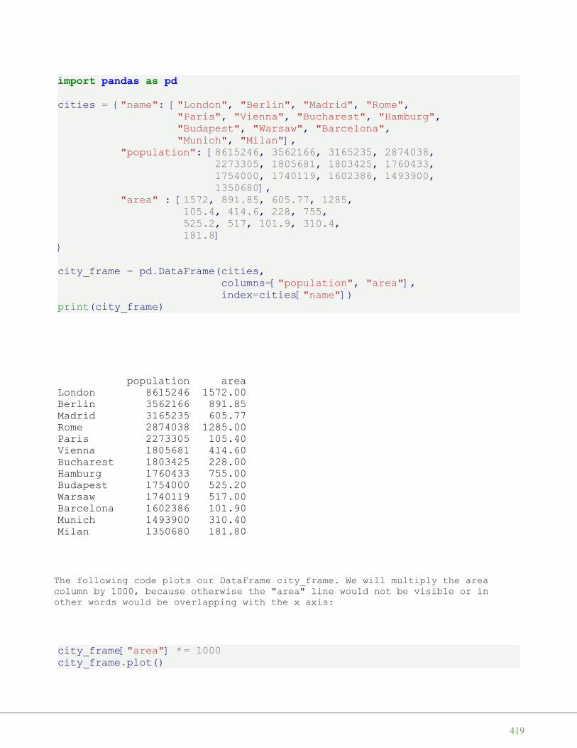
import pandas as pdcities = {"name": ["London", "Berlin", "Madrid", "Rome",

"Paris", "Vienna", "Bucharest", "Hamburg","Budapest", "Warsaw", "Barcelona","Munich", "Milan"],

"population": [8615246, 3562166, 3165235, 2874038,2273305, 1805681, 1803425, 1760433,1754000, 1740119, 1602386, 1493900,1350680],

"area" : [1572, 891.85, 605.77, 1285,105.4, 414.6, 228, 755,525.2, 517, 101.9, 310.4,181.8]

}

city_frame = pd.DataFrame(cities,columns=["population", "area"],index=cities["name"])

print(city_frame)

The following code plots our DataFrame city_frame. We will multiply the areacolumn by 1000, because otherwise the "area" line would not be visible or inother words would be overlapping with the x axis:

city_frame["area"] *= 1000city_frame.plot()

population areaLondon 8615246 1572.00Berlin 3562166 891.85Madrid 3165235 605.77Rome 2874038 1285.00Paris 2273305 105.40Vienna 1805681 414.60Bucharest 1803425 228.00Hamburg 1760433 755.00Budapest 1754000 525.20Warsaw 1740119 517.00Barcelona 1602386 101.90Munich 1493900 310.40Milan 1350680 181.80

419

This plot is not coming up to our expectations, because not all the city namesappear on the x axis. We can change this by defining the xticks explicitly with"range(len((city_frame.index))". Furthermore, we have to set use_index to True,so that we get city names and not numbers from 0 to len((city_frame.index):

city_frame.plot(xticks=range(len(city_frame.index)),use_index=True)

Now, we have a new problem. The city names are overlapping. There is remedy athand for this problem as well. We can rotate the strings by 90 degrees. Thenames will be printed vertically afterwards:

city_frame.plot(xticks=range(len(city_frame.index)),use_index=True,rot=90)

USING TWIN AXESWe multiplied the area column by 1000 to get a proper output. Instead of this, wecould have used twin axes. We will demonstrate this in the following example. We

Output: <matplotlib.axes._subplots.AxesSubplot at 0x7fe9b13f2c50>

Output: <matplotlib.axes._subplots.AxesSubplot at 0x7fe983cd72e8>

Output: <matplotlib.axes._subplots.AxesSubplot at 0x7fe98bbf6c88>

420

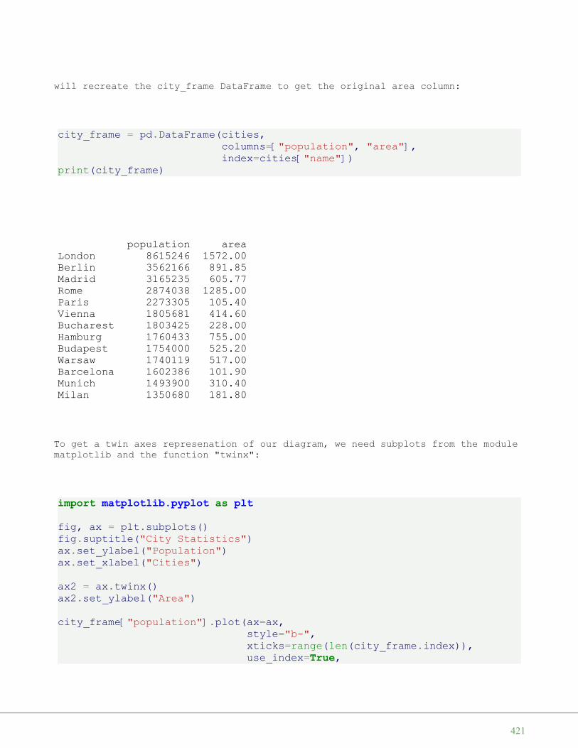
will recreate the city_frame DataFrame to get the original area column:

city_frame = pd.DataFrame(cities,columns=["population", "area"],index=cities["name"])

print(city_frame)

To get a twin axes represenation of our diagram, we need subplots from the modulematplotlib and the function "twinx":

import matplotlib.pyplot as pltfig, ax = plt.subplots()fig.suptitle("City Statistics")ax.set_ylabel("Population")ax.set_xlabel("Cities")

ax2 = ax.twinx()ax2.set_ylabel("Area")

city_frame["population"].plot(ax=ax,style="b-",xticks=range(len(city_frame.index)),use_index=True,

population areaLondon 8615246 1572.00Berlin 3562166 891.85Madrid 3165235 605.77Rome 2874038 1285.00Paris 2273305 105.40Vienna 1805681 414.60Bucharest 1803425 228.00Hamburg 1760433 755.00Budapest 1754000 525.20Warsaw 1740119 517.00Barcelona 1602386 101.90Munich 1493900 310.40Milan 1350680 181.80

421

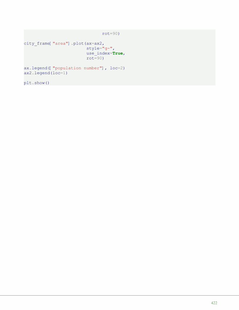
rot=90)

city_frame["area"].plot(ax=ax2,style="g-",use_index=True,rot=90)

ax.legend(["population number"], loc=2)ax2.legend(loc=1)

plt.show()

422

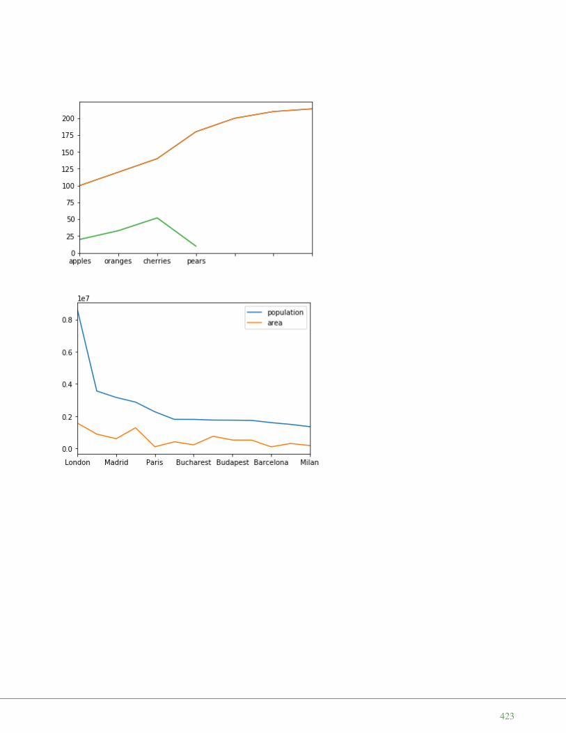
423

424

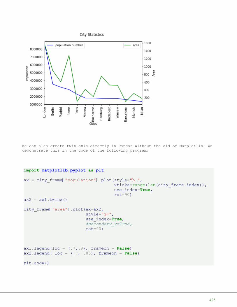
We can also create twin axis directly in Pandas without the aid of Matplotlib. Wedemonstrate this in the code of the following program:

import matplotlib.pyplot as pltax1= city_frame["population"].plot(style="b-",

xticks=range(len(city_frame.index)),use_index=True,rot=90)

ax2 = ax1.twinx()

city_frame["area"].plot(ax=ax2,style="g-",use_index=True,#secondary_y=True,rot=90)

ax1.legend(loc = (.7,.9), frameon = False)ax2.legend( loc = (.7, .85), frameon = False)plt.show()

425

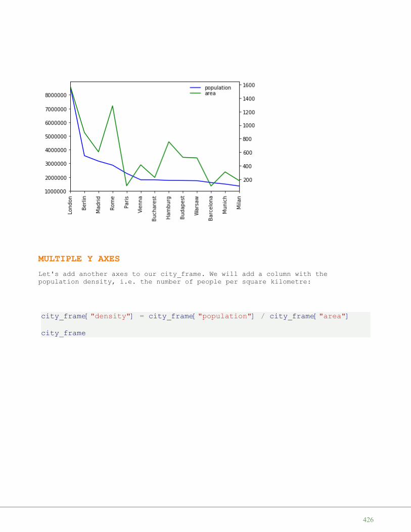
MULTIPLE Y AXESLet's add another axes to our city_frame. We will add a column with thepopulation density, i.e. the number of people per square kilometre:

city_frame["density"] = city_frame["population"] / city_frame["area"]

city_frame

426

427

Output:

population area density

London 8615246 1572.00 5480.436387

Berlin 3562166 891.85 3994.131300

Madrid 3165235 605.77 5225.143206

Rome 2874038 1285.00 2236.605447

Paris 2273305 105.40 21568.358634

Vienna 1805681 414.60 4355.236372

Bucharest 1803425 228.00 7909.758772

Hamburg 1760433 755.00 2331.699338

Budapest 1754000 525.20 3339.680122

Warsaw 1740119 517.00 3365.800774

Barcelona 1602386 101.90 15725.083415

Munich 1493900 310.40 4812.822165

Milan 1350680 181.80 7429.482948

428

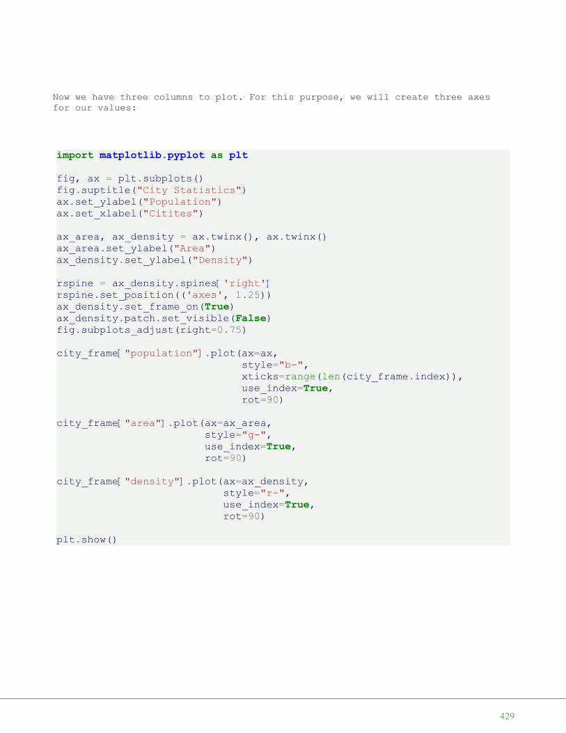
Now we have three columns to plot. For this purpose, we will create three axesfor our values:

import matplotlib.pyplot as pltfig, ax = plt.subplots()fig.suptitle("City Statistics")ax.set_ylabel("Population")ax.set_xlabel("Citites")

ax_area, ax_density = ax.twinx(), ax.twinx()ax_area.set_ylabel("Area")ax_density.set_ylabel("Density")

rspine = ax_density.spines['right']rspine.set_position(('axes', 1.25))ax_density.set_frame_on(True)ax_density.patch.set_visible(False)fig.subplots_adjust(right=0.75)

city_frame["population"].plot(ax=ax,style="b-",xticks=range(len(city_frame.index)),use_index=True,rot=90)

city_frame["area"].plot(ax=ax_area,style="g-",use_index=True,rot=90)

city_frame["density"].plot(ax=ax_density,style="r-",use_index=True,rot=90)

plt.show()

429

A MORE COMPLEX EXAMPLEWe use the previously gained knowledge in the following example. We use a filewith visitor statistics from our website python-course.eu. The content of thefile looks like this:

Month Year "Unique visitors" "Number of visits" Pages Hits Bandwidth UnitJun 2010 11 13 42 290 2.63 MBJul 2010 27 39 232 939 9.42 MBAug 2010 75 87 207 1,096 17.37 MBSep 2010 171 221 480 2,373 39.63 MB

...

Apr 2018 434,346 663,327 1,143,762 7,723,268 377.56 GBMay 2018 402,390 619,993 1,124,517 7,307,779 394.72 GBJun 2018 369,739 573,102 1,034,335 6,773,820 386.60 GBJul 2018 352,670 552,519 967,778 6,551,347 375.86 GBAug 2018 407,512 642,542 1,223,319 7,829,987 472.37 GBSep 2018 463,937 703,327 1,187,224 8,468,723 514.46 GBOct 2018 537,343 826,290 1,403,176 10,013,025 620.55 GBNov 2018 514,072 781,335 1,295,594 9,487,834 642.16 GB

430

%matplotlib inline

import pandas as pddata_path = "data1/"data = pd.read_csv(data_path + "python_course_monthly_history.txt",

quotechar='"',thousands=",",delimiter=r"\s+")

def unit_convert(x):value, unit = xif unit == "MB":

value *= 1024elif unit == "GB":

value *= 1048576 # i.e. 1024 **2return value

b_and_u= data[["Bandwidth", "Unit"]]bandwidth = b_and_u.apply(unit_convert, axis=1)

del data["Unit"]data["Bandwidth"] = bandwidth

month_year = data[["Month", "Year"]]month_year = month_year.apply(lambda x: x[0] + " " + str(x[1]),

axis=1)data["Month"] = month_yeardel data["Year"]

data.set_index("Month", inplace=True)del data["Bandwidth"]

data[["Unique visitors", "Number of visits"]].plot(use_index=True,rot=90,xticks=range(1, len(da

ta.index),4))

431

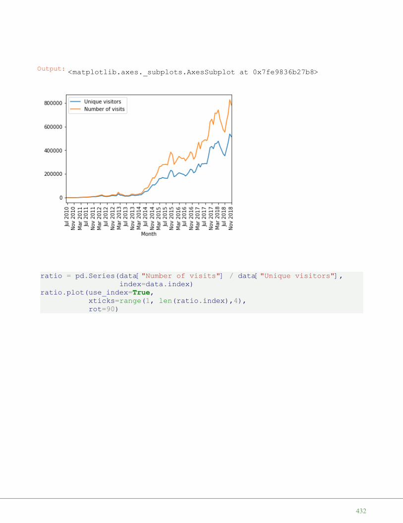
ratio = pd.Series(data["Number of visits"] / data["Unique visitors"],index=data.index)

ratio.plot(use_index=True,xticks=range(1, len(ratio.index),4),rot=90)

Output: <matplotlib.axes._subplots.AxesSubplot at 0x7fe9836b27b8>

432

CONVERTING STRING COLUMNS TO FLOATSIn the folder "data1", we have a file called

"tiobe_programming_language_usage_nov2018.txt"

with a ranking of programming languages by usage. The data has been collected andcreated by TIOBE in November 2018.

The file looks like this:

Position "Language" Percentage1 Java 16.748%2 C 14.396%3 C++ 8.282%4 Python 7.683%5 "Visual Basic .NET" 6.490%6 C# 3.952%7 JavaScript 2.655%8 PHP 2.376%9 SQL 1.844%

The percentage column contains strings with a percentage sign. We can get rid ofthis when we read in the data with read_csv. All we have to do is define aconverter function, which we to read_csv via the converters dictionary, whichcontains column names as keys and references to functions as values.

Output: <matplotlib.axes._subplots.AxesSubplot at 0x7fe9838e5860>

433

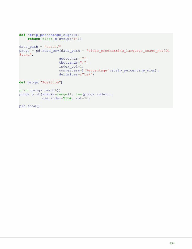
def strip_percentage_sign(x):return float(x.strip('%'))

data_path = "data1/"progs = pd.read_csv(data_path + "tiobe_programming_language_usage_nov2018.txt",

quotechar='"',thousands=",",index_col=1,converters={'Percentage':strip_percentage_sign},delimiter=r"\s+")

del progs["Position"]

print(progs.head(6))progs.plot(xticks=range(1, len(progs.index)),

use_index=True, rot=90)

plt.show()

434

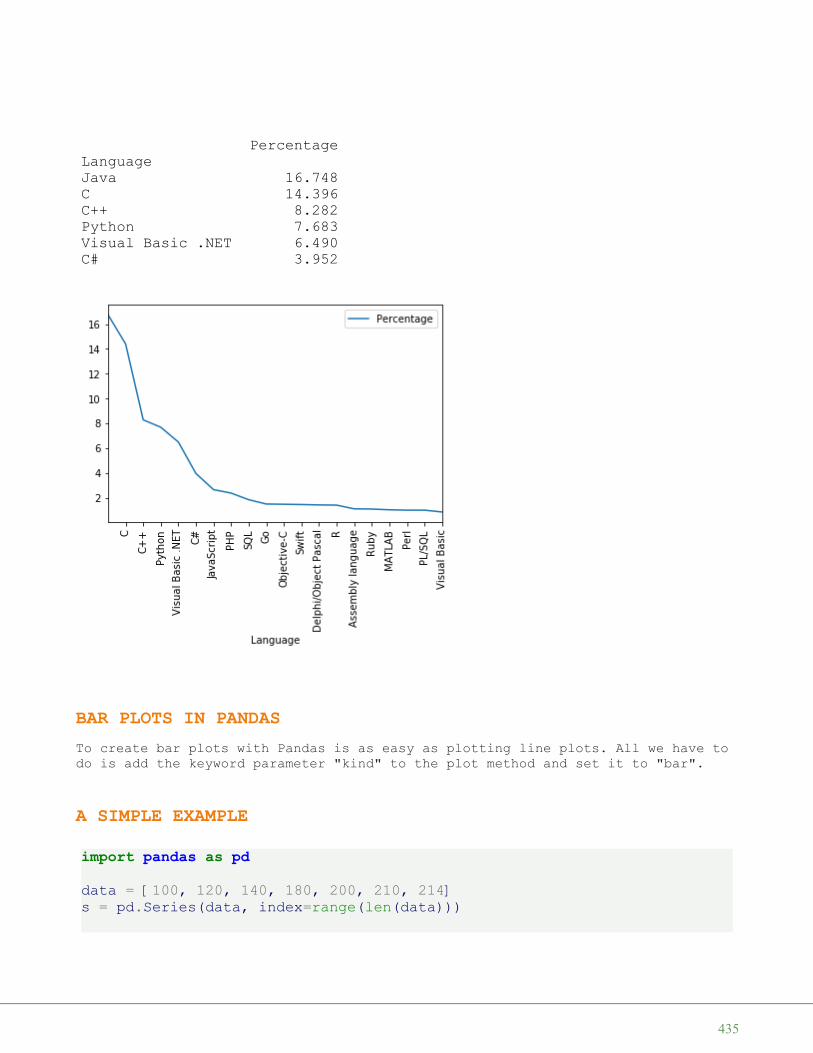
BAR PLOTS IN PANDASTo create bar plots with Pandas is as easy as plotting line plots. All we have todo is add the keyword parameter "kind" to the plot method and set it to "bar".

A SIMPLE EXAMPLEimport pandas as pddata = [100, 120, 140, 180, 200, 210, 214]s = pd.Series(data, index=range(len(data)))

PercentageLanguageJava 16.748C 14.396C++ 8.282Python 7.683Visual Basic .NET 6.490C# 3.952

435

s.plot(kind="bar")

BAR PLOT FOR PROGRAMMING LANGUAGE USAGELet's get back to our programming language ranking. We will printout now a barplot of the six most used programming languages:

progs[:6].plot(kind="bar")

Output: <matplotlib.axes._subplots.AxesSubplot at 0x7fe98349a5c0>

436

Now the whole chart with all programming languages:

progs.plot(kind="bar")

Output: <matplotlib.axes._subplots.AxesSubplot at 0x7fe983ac05c0>

437

COLORIZE A BAR PLOTIt is possible to colorize the bars indivually by assigning a list to the keywordparameter color:

my_colors = ['b', 'r', 'c', 'y', 'g', 'm']progs[:6].plot(kind="bar",

color=my_colors)

Output: <matplotlib.axes._subplots.AxesSubplot at 0x7fe983a84208>

438

PIE CHART DIAGRAMS IN PANDASA simple example:

import pandas as pdfruits = ['apples', 'pears', 'cherries', 'bananas']series = pd.Series([20, 30, 40, 10],

index=fruits,name='series')

series.plot.pie(figsize=(6, 6))

Output: <matplotlib.axes._subplots.AxesSubplot at 0x7fe9834509e8>

439

fruits = ['apples', 'pears', 'cherries', 'bananas']

series = pd.Series([20, 30, 40, 10],index=fruits,name='series')

explode = [0, 0.10, 0.40, 0.7]series.plot.pie(figsize=(6, 6),

explode=explode)

Output: <matplotlib.axes._subplots.AxesSubplot at 0x7fe9832fe048>

440

We will replot the previous bar plot as a pie chart plot:

import matplotlib.pyplot as pltmy_colors = ['b', 'r', 'c', 'y', 'g', 'm']progs.plot.pie(subplots=True,

legend=False)

Output: <matplotlib.axes._subplots.AxesSubplot at 0x7fe983370198>

441

It looks ugly that we see the y label "Percentage" inside our pie plot. We canremove it by calling "plt.ylabel('')"

import matplotlib.pyplot as pltmy_colors = ['b', 'r', 'c', 'y', 'g', 'm']progs.plot.pie(subplots=True,

legend=False)plt.ylabel('')

Output: array([<matplotlib.axes._subplots.AxesSubplot object at 0x7fe9832440b8>], dtype=object)

442

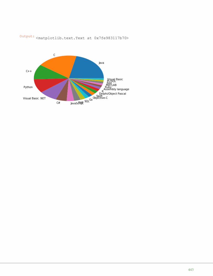
Output: <matplotlib.text.Text at 0x7fe983117b70>

443

P Y T H O N , D A T E A N D T I M E

INTRODUCTIONPython provides richfunctionalities for dealingwith date and time data. Thestandard libraries containsthe modules

• time• calendar• datetime

These modules supply classesfor manipulating dates andtimes in both simple andcomplex ways.

Especially, the datetime classwill be very important for thetimeseries of Pandas.

PYTHON STANDARDMODULES FOR TIME DATAThe most important modules ofPython dealing with time arethe modules time ,calendar and datetime .

The datetime module providesvarious classes, methods andfunctions to deal with dates,times, and time intervals.

The datetime module providesthe following classes:

• The instances of the date class represent dates, whereas the year canrange between 1 and 9999.

• The instances of the datetime class are made up both by a date and atime.

• The time class implements time objects.• The timedelta class is used to hold the differences between two times

or two date objects.• The tzinfo class is used to implement timezone support for time and

datetime objects.

Let's start with a date object.

444

THE DATE CLASSfrom datetime import date

x = date(1993, 12, 14)print(x)

We can instantiate dates in the range from January 1, 1 to December 31, 9999.This can be inquired from the attributes min and max :

from datetime import date

print(date.min)print(date.max)

We can apply various methods to the date instance above.The method toordinal returns the proleptic Gregorian ordinal. The prolepticGregorian calendar is produced by extending the Gregorian calendar backward todates preceding its official introduction in 1582. January 1 of year 1 is day 1.

x.toordinal()

1993-12-14

0001-01-019999-12-31

445

It is possible to calculate a date from a ordinal by using the class method"fromordinal":

date.fromordinal(727911)

If you want to know the weekday of a certain date, you can calculate it by usingthe method weekday:

x.weekday()

date.today()

We can access the day, month and year with attributes:

Output: 727911

Output: datetime.date(1993, 12, 14)

Output: 1

Output: datetime.date(2017, 4, 12)

446

print(x.day)print(x.month)print(x.year)

THE TIME CLASSThe time class is similarly organized than the date class.

from datetime import time

t = time(15, 6, 23)print(t)

The possible times range between:

print(time.min)print(time.max)

14121993

15:06:23

00:00:0023:59:59.999999

447

Accessing 'hour', 'minute' and 'second':

t.hour, t.minute, t.second

Each component of a time instance can be changed by using 'replace':

t = t.replace(hour=11, minute=59)t

We can render a date as a C-style like string, corresponding to the C ctimefunction:

x.ctime()

THE DATETIME CLASSThe datetime module provides us with functions and methods for manipulatingdates and times. It supplies functionalities for date and time arithmetic, i.e.

Output: (15, 6, 23)

Output: datetime.time(11, 59, 23)

Output: 'Tue Dec 14 00:00:00 1993'

448

addition and subtraction. Another focus of the implementation is on attributeextraction for output manipulation and formatting.

There are two kinds of date and time objects:

• naive• aware

If a time or date object is naive it doesn't contain information to compare orlocate itself relative to other date or time objects. The semantics, if such anaive object belongs to a certain time zone, e.g. Coordinated Universal Time(UTC), local time, or some other timezone is contained in the logic of theprogram.

An aware object on the other hand possesses knowledge of the time zone it belongsto or the daylight saving time information. This way it can locate itselfrelative to other aware objects.

How can you tell if a datetime object t is aware?

t is aware if t.tzinfo is not None and t.tzinfo.utcoffset(t) is not None.Both conditions have to be fulfilled

On the other hand an object t is naive if t.tzinfo is None ort.tzinfo.utcoffset(t) is None

Let's create a datetime object:

from datetime import datetimet = datetime(2017, 4, 19, 16, 31, 0)t

t is naive, because the following is True:

t.tzinfo == None

Output: datetime.datetime(2017, 4, 19, 16, 31)

449

We will create an aware datetime object from the current date. For this purposewe need the module pytz. pytz is a module, which brings the Olson tz databaseinto Python. The Olson timezones are nearly completely supported by this module.

from datetime import datetimeimport pytzt = datetime.now(pytz.utc)

We can see that both t.tzinfo and t.tzinfo.utcoffset(t) are different from None,so t is an aware object:

t.tzinfo, t.tzinfo.utcoffset(t)

from datetime import datetime, timedelta as deltandays = 15start = datetime(1991, 4, 30)dates = [start - delta(days=x) for x in range(0, ndays)]dates

Output: True

Output: (<UTC>, datetime.timedelta(0))

450

DIFFERENCES BETWEEN TIMESLet's see what happens, if we subtract to datetime objects:

from datetime import datetime

delta = datetime(1993, 12, 14) - datetime(1991, 4, 30)delta, type(delta)

The result of the subtraction of the two datetime objects is a timedelta object,as we can see from the example above.

We can get information about the number of days elapsed by using the attribute'days':

delta.days

Output: [datetime.datetime(1991, 4, 30, 0, 0),datetime.datetime(1991, 4, 29, 0, 0),datetime.datetime(1991, 4, 28, 0, 0),datetime.datetime(1991, 4, 27, 0, 0),datetime.datetime(1991, 4, 26, 0, 0),datetime.datetime(1991, 4, 25, 0, 0),datetime.datetime(1991, 4, 24, 0, 0),datetime.datetime(1991, 4, 23, 0, 0),datetime.datetime(1991, 4, 22, 0, 0),datetime.datetime(1991, 4, 21, 0, 0),datetime.datetime(1991, 4, 20, 0, 0),datetime.datetime(1991, 4, 19, 0, 0),datetime.datetime(1991, 4, 18, 0, 0),datetime.datetime(1991, 4, 17, 0, 0),datetime.datetime(1991, 4, 16, 0, 0)]

Output: (datetime.timedelta(959), datetime.timedelta)

451

t1 = datetime(2017, 1, 31, 14, 17)t2 = datetime(2015, 12, 15, 16, 59)delta = t1 - t2delta.days, delta.seconds

It is possible to add or subtract a timedelta to adatetime object to calculate a new datetime object by adding or subtracting thedelta in days:

from datetime import datetime, timedeltad1 = datetime(1991, 4, 30)d2 = d1 + timedelta(10)print(d2)print(d2 - d1)

d3 = d1 - timedelta(100)print(d3)d4 = d1 - 2 * timedelta(50)print(d4)

Output: 959

Output: (412, 76680)

1991-05-10 00:00:0010 days, 0:00:001991-01-20 00:00:001991-01-20 00:00:00

452

It is also possible to add days and minutes to t datetime object:

from datetime import datetime, timedeltad1 = datetime(1991, 4, 30)d2 = d1 + timedelta(10,100)print(d2)print(d2 - d1)

CONVERT DATETIME OBJECTS TO STRINGSThe easiest way to convert a datetime object into a string consists in using str.

s = str(d1)s

CONVERSION WITH STRFTIMEThe method call datetime.strftime(format) return a string representing the dateand time, controlled by an explicit format string. A complete list of formattingdirectives can be found at strftime:

print(d1.strftime('%Y-%m-%d'))print("weekday: " + d1.strftime('%a'))print("weekday as a full name: " + d1.strftime('%A'))

1991-05-10 00:01:4010 days, 0:01:40

Output: '1991-04-30 00:00:00'

453

# Weekday as a decimal number, where 0 is Sunday# and 6 is Saturdayprint("weekday as a decimal number: " + d1.strftime('%w'))

Formatting months:

# Day of the month as a zero-padded decimal number.# 01, 02, ..., 31print(d1.strftime('%d'))# Month as locale’s abbreviated name.# Jan, Feb, ..., Dec (en_US);# Jan, Feb, ..., Dez (de_DE)print(d1.strftime('%b'))

# Month as locale’s full name.# January, February, ..., December (en_US);# Januar, Februar, ..., Dezember (de_DE)print(d1.strftime('%B'))

# Month as a zero-padded decimal number.# 01, 02, ..., 12print(d1.strftime('%m'))

1991-04-30weekday: Tueweekday as a full name: Tuesdayweekday as a decimal number: 2

30AprApril04

454

CREATING DATETIME OBJECTS FROM STRINGSWe can use strptime to create new datetime object by parsing a string containinga data and time. The arguments of strptime are the string to be parsed and aformat specification.

from datetime import datetimet = datetime.strptime("30 Nov 00", "%d %b %y")print(t)

dt = "2007-03-04T21:08:12"datetime.strptime( dt, "%Y-%m-%dT%H:%M:%S" )

dt = '12/24/1957 4:03:29 AM'dt = datetime.strptime(dt, '%m/%d/%Y %I:%M:%S %p')dt

We can create an English date string on a Linux machine with the Shell command

LC_ALL=en_EN.utf8 date

2000-11-30 00:00:00

Output: datetime.datetime(2007, 3, 4, 21, 8, 12)

Output: datetime.datetime(1957, 12, 24, 4, 3, 29)

455

dt = 'Wed Apr 12 20:29:53 CEST 2017'dt = datetime.strptime(dt, '%a %b %d %H:%M:%S %Z %Y')print(dt)

Though datetime.strptime is an easy way to parse a date with a known format, itcan be quote complicated and cumbersome to write every time a new specificationstring for new date formats.

Using the parse method from dateutil.parser:

from dateutil.parser import parse

parse('2011-01-03')

parse('Wed Apr 12 20:29:53 CEST 2017')

2017-04-12 20:29:53

Output: datetime.datetime(2011, 1, 3, 0, 0)

Output: datetime.datetime(2017, 4, 12, 20, 29, 53, tzinfo=tzlocal())

456

P Y T H O N , P A N D A S A N D T I M E S E R I E S

INTRODUCTIONOur next chapter of our PandasTutorial deals with timeseries. A time series is aseries of data points, whichare listed (or indexed) intime order. Usually, a timeseries is a sequence ofvalues, which are equallyspaced points in time.Everything which consists ofmeasured data connected withthe corresponding time can beseen as a time series.Measurements can be takenirregularly, but in most casestime series consist of fixedfrequencies. This means thatdata is measured or taken in aregular pattern, i.e. forexample every 5 milliseconds,every 10 seconds, or very hour.Often time series are plotted as line charts.

In this chapter of our tutorial on Python with Pandas, we will introduce thetools from Pandas dealing with time series. You will learn how to cope with largetime series and how modify time series.

Before you continue reading it might be useful to go through our tutorial on thestandard Python modules dealing with time processing, i.e. datetime, time andcalendar:

TIME SERIES IN PANDAS AND PYTHONWe could define a Pandas Series, which is built with an index consisting of timestamps.

import numpy as npimport pandas as pdfrom datetime import datetime, timedelta as deltandays = 10start = datetime(2017, 3, 31)dates = [start - delta(days=x) for x in range(0, ndays)]

457

values = [25, 50, 15, 67, 70, 9, 28, 30, 32, 12]

ts = pd.Series(values, index=dates)ts

Let's check the type of the newly created time series:

type(ts)

What does the index of a time series look like? Let's see:

ts.index

Output: 2017-03-31 252017-03-30 502017-03-29 152017-03-28 672017-03-27 702017-03-26 92017-03-25 282017-03-24 302017-03-23 322017-03-22 12dtype: int64

Output: pandas.core.series.Series

458

We will create now another time series:

values2 = [32, 54, 18, 61, 72, 19, 21, 33, 29, 17]

ts2 = pd.Series(values2, index=dates)

It is possible to use arithmetic operations on time series like we did with otherseries. We can for example add the two previously created time series:

ts + ts2

Arithmetic mean between both Series, i.e. the values of the series:

Output: DatetimeIndex(['2017-03-31', '2017-03-30', '2017-03-29', '2017-03-28',

'2017-03-27', '2017-03-26', '2017-03-25', '2017-03-24',

'2017-03-23', '2017-03-22'],dtype='datetime64[ns]', freq=None)

Output: 2017-03-31 572017-03-30 1042017-03-29 332017-03-28 1282017-03-27 1422017-03-26 282017-03-25 492017-03-24 632017-03-23 612017-03-22 29dtype: int64

459

(ts + ts2) / 2

As with other series the indices don't have to be the same.

import pandas as pdfrom datetime import datetime, timedelta as delta

ndays = 10

start = datetime(2017, 3, 31)dates = [start - delta(days=x) for x in range(0, ndays)]

start2 = datetime(2017, 3, 26)dates2 = [start2 - delta(days=x) for x in range(0, ndays)]

values = [25, 50, 15, 67, 70, 9, 28, 30, 32, 12]values2 = [32, 54, 18, 61, 72, 19, 21, 33, 29, 17]

ts = pd.Series(values, index=dates)ts2 = pd.Series(values2, index=dates2)

ts + ts2

Output: 2017-03-31 28.52017-03-30 52.02017-03-29 16.52017-03-28 64.02017-03-27 71.02017-03-26 14.02017-03-25 24.52017-03-24 31.52017-03-23 30.52017-03-22 14.5dtype: float64

460

CREATE DATE RANGESThe date_range method of the pandas module can be used to generate aDatetimeIndex:

import pandas as pdindex = pd.date_range('12/24/1970', '01/03/1971')index

We have passed a start and an end date to date_range in our previous example. Itis also possible to pass only a start or an end date to the function. In thiscase, we have to determine the number of periods to generate by setting thekeyword parameter 'periods':

Output: 2017-03-17 NaN2017-03-18 NaN2017-03-19 NaN2017-03-20 NaN2017-03-21 NaN2017-03-22 84.02017-03-23 93.02017-03-24 48.02017-03-25 82.02017-03-26 41.02017-03-27 NaN2017-03-28 NaN2017-03-29 NaN2017-03-30 NaN2017-03-31 NaNdtype: float64

Output: DatetimeIndex(['1970-12-24', '1970-12-25', '1970-12-26', '1970-12-27',

'1970-12-28', '1970-12-29', '1970-12-30', '1970-12-31',

'1971-01-01', '1971-01-02', '1971-01-03'],dtype='datetime64[ns]', freq='D')

461

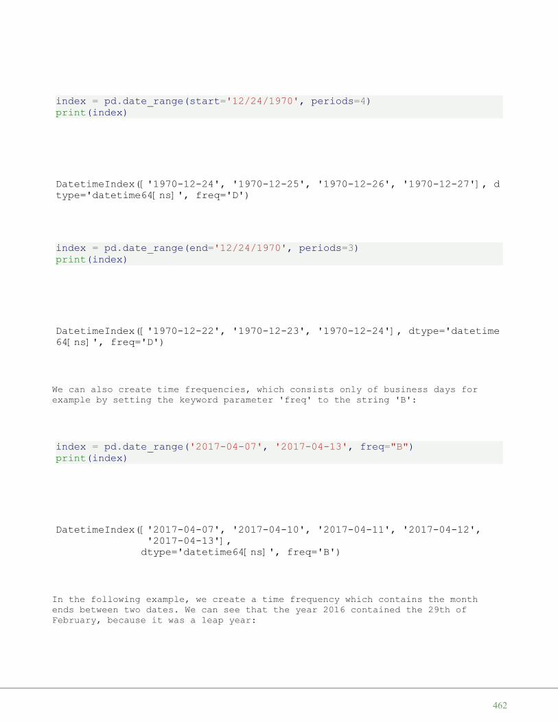
index = pd.date_range(start='12/24/1970', periods=4)print(index)

index = pd.date_range(end='12/24/1970', periods=3)print(index)

We can also create time frequencies, which consists only of business days forexample by setting the keyword parameter 'freq' to the string 'B':

index = pd.date_range('2017-04-07', '2017-04-13', freq="B")print(index)

In the following example, we create a time frequency which contains the monthends between two dates. We can see that the year 2016 contained the 29th ofFebruary, because it was a leap year:

DatetimeIndex(['1970-12-24', '1970-12-25', '1970-12-26', '1970-12-27'], dtype='datetime64[ns]', freq='D')

DatetimeIndex(['1970-12-22', '1970-12-23', '1970-12-24'], dtype='datetime64[ns]', freq='D')

DatetimeIndex(['2017-04-07', '2017-04-10', '2017-04-11', '2017-04-12','2017-04-13'],

dtype='datetime64[ns]', freq='B')

462

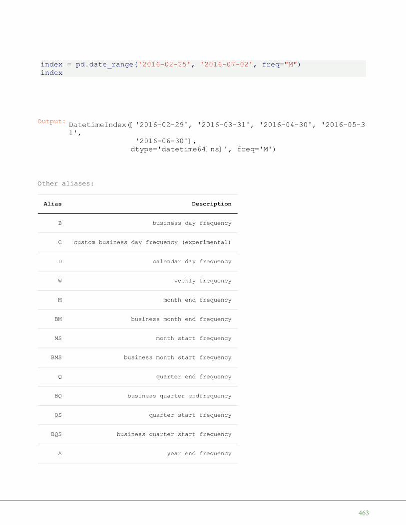
index = pd.date_range('2016-02-25', '2016-07-02', freq="M")index

Other aliases:

Alias Description

B business day frequency

C custom business day frequency (experimental)

D calendar day frequency

W weekly frequency

M month end frequency

BM business month end frequency

MS month start frequency

BMS business month start frequency

Q quarter end frequency

BQ business quarter endfrequency

QS quarter start frequency

BQS business quarter start frequency

A year end frequency

Output: DatetimeIndex(['2016-02-29', '2016-03-31', '2016-04-30', '2016-05-31',

'2016-06-30'],dtype='datetime64[ns]', freq='M')

463

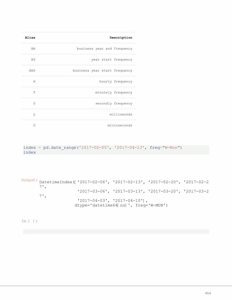
Alias Description

BA business year end frequency

AS year start frequency

BAS business year start frequency

H hourly frequency

T minutely frequency

S secondly frequency

L milliseonds

U microseconds

index = pd.date_range('2017-02-05', '2017-04-13', freq="W-Mon")index

In [ ]:

Output: DatetimeIndex(['2017-02-06', '2017-02-13', '2017-02-20', '2017-02-27',

'2017-03-06', '2017-03-13', '2017-03-20', '2017-03-27',

'2017-04-03', '2017-04-10'],dtype='datetime64[ns]', freq='W-MON')

464

E X P E N S E S A N D I N C O M E E X A M P L E

In this chapter of our Pandastutorial we will deal withsimple Expense and Incometables for private usage. Somesay that if you want to manageyour money successfully youwill have to track your incomeand expenses. Monitoring theflow of money is important tounderstand your financialsituation. You need to knowexactly how much is coming inand going out. This article isnot meant to convince you ofthe necessity of doing this.The main focus is rather onthe possibilities offered byPython and Pandas to programthe necessary tools.

We will start with a smallexample, suitable for privatepurposes and the followingchapter of our tutorialcontinues with a moreextensive example suitable forsmall businesses.

PRIVATE BUDGETING WITHPYTHON AND PANDASLet us assume that you have already a csv file containing your expenses andincome over a certain period of time. This journal may look like this:

Date;Description;Category;Out;In2020-06-02;Salary Frank;Income;0;4896.442020-06-03;supermarket;food and beverages;132.40;02020-06-04;Salary Laura;Income;0;4910.142929-06-04;GreenEnergy Corp., (electricity);utility;87.34;02020-06-09;water and sewage;utility;60.56;02020-06-10;Fitness studio, Jane;health and sports;19.00;02020-06-11;payment to bank;monthly redemption payment;1287.43;02020-06-12;LeGourmet Restaurant;restaurants and hotels;145.00;02020-06-13;supermarket;food and beverages;197.42;02020-06-13;Pizzeria da Pulcinella;restaurants and hotels;60.00;02020-06-26;supermarket;food and beverages;155.42;02020-06-27;theatre tickets;education and culture;125;0

465

2020-07-02;Salary Frank;Income;0;4896.442020-07-03;supermarket;food and beverages;147.90;02020-07-05;Salary Laura;Income;0;4910.142020-07-08;Golf Club, yearly payment;health and sports;612.18;02020-07-09;house insurance;insurances and taxes;167.89;02020-07-10;Fitness studio, Jane;health and sports;19.00;02020-07-10;supermarket;food and beverages;144.12;02020-07-11;payment to bank;monthly redemption payment;1287.43;02020-07-18;supermarket;food and beverages;211.24;02020-07-13;Pizzeria da Pulcinella;restaurants and hotels;33.00;02020-07-23;Cinema;education and culture;19;02020-07-25;supermarket;food and beverages;186.11;0

The above mentioned csv file is saved under the name expenses_and_income.csv inthe folder data . It is easy to read it in with Pandas as we can see in ourchapter Pandas Data Files:

import pandas as pdexp_inc = pd.read_csv("data1/expenses_and_income.csv", sep=";")exp_inc

466

467

Output:

Date Description Category Out In

0 2020-06-02 Salary Frank Income 0.00 4896.44

1 2020-06-03 supermarket food andbeverages 132.40 0.00

2 2020-06-04 Salary Laura Income 0.00 4910.14

3 2929-06-04 GreenEnergy Corp.,(electricity) utility 87.34 0.00

4 2020-06-09 water and sewage utility 60.56 0.00

5 2020-06-10 Fitness studio, Jane health and sports 19.00 0.00

6 2020-06-11 payment to bankmonthly

redemptionpayment

1287.43 0.00

7 2020-06-12 LeGourmet Restaurant restaurants andhotels 145.00 0.00

8 2020-06-13 supermarket food andbeverages 197.42 0.00

9 2020-06-13 Pizzeria daPulcinella

restaurants andhotels 60.00 0.00

10 2020-06-26 supermarket food andbeverages 155.42 0.00

468

Date Description Category Out In

11 2020-06-27 theatre tickets education andculture 125.00 0.00

12 2020-07-02 Salary Frank Income 0.00 4896.44

13 2020-07-03 supermarket food andbeverages 147.90 0.00

14 2020-07-05 Salary Laura Income 0.00 4910.14

15 2020-07-08 Golf Club, yearlypayment health and sports 612.18 0.00

16 2020-07-09 house insurance insurances andtaxes 167.89 0.00

17 2020-07-10 Fitness studio, Jane health and sports 19.00 0.00

18 2020-07-10 supermarket food andbeverages 144.12 0.00

19 2020-07-11 payment to bankmonthly

redemptionpayment

1287.43 0.00

20 2020-07-18 supermarket food andbeverages 211.24 0.00

21 2020-07-13 Pizzeria daPulcinella

restaurants andhotels 33.00 0.00

22 2020-07-23 Cinema education andculture 19.00 0.00

469

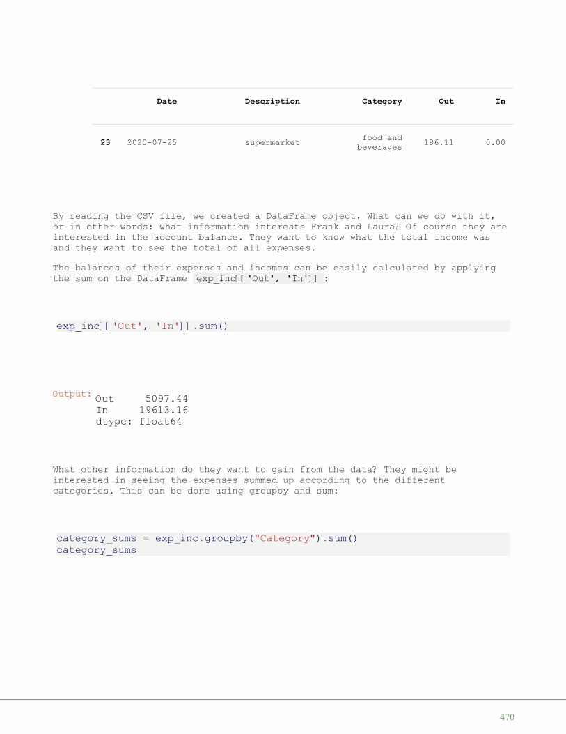
By reading the CSV file, we created a DataFrame object. What can we do with it,or in other words: what information interests Frank and Laura? Of course they areinterested in the account balance. They want to know what the total income wasand they want to see the total of all expenses.

The balances of their expenses and incomes can be easily calculated by applyingthe sum on the DataFrame exp_inc[['Out', 'In']] :

exp_inc[['Out', 'In']].sum()

What other information do they want to gain from the data? They might beinterested in seeing the expenses summed up according to the differentcategories. This can be done using groupby and sum:

category_sums = exp_inc.groupby("Category").sum()category_sums

Date Description Category Out In

23 2020-07-25 supermarket food andbeverages 186.11 0.00

Output: Out 5097.44In 19613.16dtype: float64

470

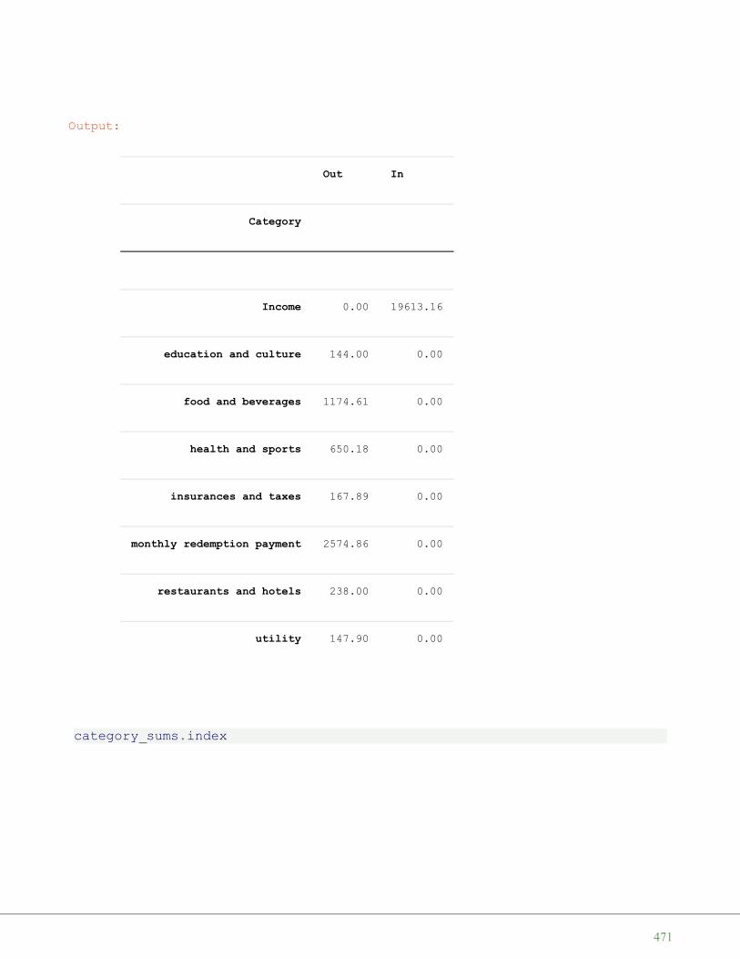
category_sums.index

Output:

Out In

Category

Income 0.00 19613.16

education and culture 144.00 0.00

food and beverages 1174.61 0.00

health and sports 650.18 0.00

insurances and taxes 167.89 0.00

monthly redemption payment 2574.86 0.00

restaurants and hotels 238.00 0.00

utility 147.90 0.00

471

import matplotlib.pyplot as pltax = category_sums.plot.bar(y="Out")plt.xticks(rotation=45)

We can also display this as a pie chart:

Output: Index(['Income', 'education and culture', 'food and beverages','health and sports', 'insurances and taxes','monthly redemption payment', 'restaurants and hotels', 'uti

lity'],dtype='object', name='Category')

Output: (array([0, 1, 2, 3, 4, 5, 6, 7]), <a list of 8 Text xticklabel objects>)

472

ax = category_sums.plot.pie(y="Out")ax.legend(loc="upper left", bbox_to_anchor=(1.5, 1))

Alternatively, we can create the same pie plot with the following code:

ax = category_sums["Out"].plot.pie()ax.legend(loc="upper left", bbox_to_anchor=(1.5, 1))

Output: <matplotlib.legend.Legend at 0x7fe20d953fd0>

473

If you imagine that you will have to type in all the time category names like"household goods and service" or "rent and mortgage interest", you will agreethat it is very likely to have typos in your journal of expenses and income.

So it will be a good idea to use numbers (account numbers) for your categories.The following categories are available in our example.

The following categories are provided:

Category Account Number

rent and mortgage interest 200

insurances and taxes 201

food and beverages 202

education and culture 203

transport 204

health and sports 205

household goods and services 206

Output: <matplotlib.legend.Legend at 0x7fe20d90c810>

474

Category Account Number

clothing 207

communications 208

restaurants and hotels 209

utility ( heating, electricity, water, and garbage) 210

other expenses 211

income 400

We can implement this as a dictionary mapping categories into account numbers:

category2account = {'monthly redemption payment': '200','insurances and taxes': '201','food and beverages': '202','education and culture': '203','transport': '204','health and sports': '205','household goods and services': '206','clothing': '207','communications': '208','restaurants and hotels': '209','utility': '210','other expenses': '211','Income': '400'}

The next step is to replace our "clumsy" category names with the account numbers.The replace method of DataFrame is ideal for this purpose. We can replace allthe occurrences of the category names in our DataFrame by the correspondingaccount names:

exp_inc.replace(category2account, inplace=True)exp_inc.rename(columns={"Category": "Accounts"}, inplace=True)exp_inc[:5]

475

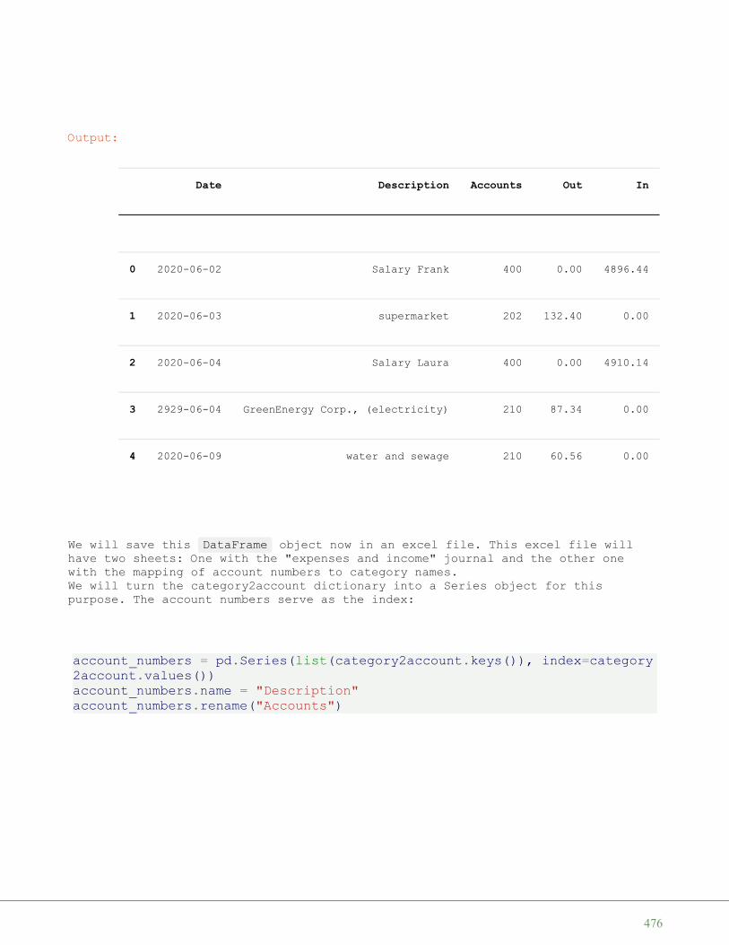
We will save this DataFrame object now in an excel file. This excel file willhave two sheets: One with the "expenses and income" journal and the other onewith the mapping of account numbers to category names.We will turn the category2account dictionary into a Series object for thispurpose. The account numbers serve as the index:

account_numbers = pd.Series(list(category2account.keys()), index=category2account.values())account_numbers.name = "Description"account_numbers.rename("Accounts")

Output:

Date Description Accounts Out In

0 2020-06-02 Salary Frank 400 0.00 4896.44

1 2020-06-03 supermarket 202 132.40 0.00

2 2020-06-04 Salary Laura 400 0.00 4910.14

3 2929-06-04 GreenEnergy Corp., (electricity) 210 87.34 0.00

4 2020-06-09 water and sewage 210 60.56 0.00

476

exp_inc.insert(1, "accounts", account_numbers)

with pd.ExcelWriter('data1/expenses_and_income_2020.xlsx') as writer:account_numbers.to_excel(writer, "account numbers")exp_inc.to_excel(writer, "journal")writer.save()

Output: 200 monthly redemption payment201 insurances and taxes202 food and beverages203 education and culture204 transport205 health and sports206 household goods and services207 clothing208 communications209 restaurants and hotels210 utility211 other expenses400 IncomeName: Accounts, dtype: object

477

N E T I N C O M E M E T H O D E X A M P L E

The Net Income Method (inGermany known asEinnahmeüberschussrechnung,EÜR) is a simplified profitdetermination method. UnderGerman law, self-employedpersons such as doctors,lawyers, architects and othershave the choice of submittingannual accounts or using thesimple net income method. Whatwe present in this chapter ofour Pandas tutorial will notonly be interesting for smallcompanies, especially inGermany and EU countries, butalso for other countries inthe world as well.

We are mainly interested inintroducing the different waysin which pandas and python can solve such problems. We show what it is all aboutto monitor the flow of money and in this way to better understand the financialsituation. The algorithms can also be used for tax purposes. But be warned, thisis a very general treatment of the matter and needs to be adjusted to the actualtax situation in your country. Although it is mainly based on German law, wecannot guarantee its accuracy! So, before you actually use it, you have to makesure that it is suitable for your situation and the tax laws of your country.

Very often a Microsoft Excel file is used for mainting a journal file of thefinancial transactions.In the data1 folder there is a file that contains an Excel filenet_income_method_2020.xlsx with the accounting data of a fictitious company.We could have used simple texts files like csv as well.

JOURNAL FILEThis excel document contains two data sheets: One with the actual data "journal"and one with the name "account numbers", which contains the mapping from theaccount numbers to the description.

478

We will read this excel file into two DataFrame objects:

479

import pandas as pdwith pd.ExcelFile("data1/net_income_method_2020.xlsx") as xl:

accounts2descr = xl.parse("account numbers",index_col=0)

journal = xl.parse("journal",index_col=0,

)

journal.index = pd.to_datetime(journal.index)journal.index

480

The first one is the tab "account numbers" which contains the mapping from theaccount numbers to the description of the accounts:

Output: DatetimeIndex(['2020-04-02', '2020-04-02', '2020-04-02', '2020-04-02',

'2020-04-02', '2020-04-02', '2020-04-05', '2020-04-05',

'2020-04-05', '2020-04-05', '2020-04-09', '2020-04-09',

'2020-04-10', '2020-04-10', '2020-04-10', '2020-04-10',

'2020-04-10', '2020-04-10', '2020-04-13', '2020-04-13',

'2020-04-13', '2020-04-26', '2020-04-26', '2020-04-26',

'2020-04-26', '2020-04-27', '2020-05-03', '2020-05-03',

'2020-05-03', '2020-05-03', '2020-05-05', '2020-05-05',

'2020-05-08', '2020-05-09', '2020-05-10', '2020-05-11',

'2020-05-11', '2020-05-11', '2020-05-11', '2020-05-11',

'2020-05-13', '2020-05-18', '2020-05-25', '2020-05-25',

'2020-06-01', '2020-06-02', '2020-06-03', '2020-06-03',

'2020-06-04', '2020-06-04', '2020-06-09', '2020-06-10',

'2020-06-10', '2020-06-11', '2020-06-11', '2020-06-11',

'2020-06-11', '2020-06-11', '2020-06-12', '2020-06-13',

'2020-06-13', '2020-06-26', '2020-06-26', '2020-06-27',

'2020-07-02', '2020-07-03', '2020-07-05', '2020-07-05',

'2020-07-08', '2020-07-09', '2020-07-10', '2020-07-10',

'2020-07-10', '2020-07-10', '2020-07-10', '2020-07-10',

'2020-07-11', '2020-07-11', '2020-07-13', '2020-07-18',

'2020-07-23', '2020-07-23', '2020-07-25', '2020-07-25',

'2020-07-27', '2020-07-26', '2020-07-28'],dtype='datetime64[ns]', name='date', freq=None)

481

accounts2descr

482

483

Output:

description

account

4400 revenue plant Munich

4401 revenue plant Frankfurt

4402 revenue plant Berlin

2010 souvenirs

2020 clothes

2030 other articles

2050 books

2100 insurances

2200 wages

2300 loans

2400 hotels

2500 petrol

484

The second data sheet "journal" contains the actual journal entries:

journal[:10]

description

account

2600 telecommunication

2610 internet

485

Output:

accountnumber

documentnumber description tax

rategrossamount

date

2020-04-02 4402 8983233038 Zurkan, Köln 19 4105.98

2020-04-02 2010 57550799 Birmann,Souvenirs 19 -1890.00

2020-04-02 2200 14989004 wages 0 -17478.23

2020-04-02 2500 12766279 Filling Station,Petrol 19 -89.40

2020-04-02 4400 3733462359 EnergyCom,Hamburg 19 4663.54

2020-04-02 4402 7526058231 Enoigo,Strasbourg 19 2412.82

2020-04-05 4402 1157284466 Qbooks, Frankfurt 7 2631.42

2020-04-05 4402 7009463592 Qbooks, Köln 7 3628.45

2020-04-05 2020 68433353 Jamdon, Clothes 19 -1900.00

2020-04-05 2010 53353169 Outleg, Souvenirs 19 -2200.00

486

There are many ways to analyze this data. We can for example sum up all theaccounts:

account_sums = journal[["account number", "gross amount"]].groupby("account number").sum()account_sums

487

488

Output:

gross amount

account number

2010 -4090.00

2020 -10500.80

2030 -1350.00

2050 -900.00

2100 -612.00

2200 -69912.92

2300 -18791.92

2400 -1597.10

2500 -89.40

2600 -492.48

2610 -561.00

4400 37771.84

489

ACCOUNT CHARTSWhat about showing a pie chart of these sums? We encounter one problem: Piecharts cannot contain negative values. However this is not a real problem. We cansplit the accounts into income and expense accounts. Of course, this correspondsmore to what we really want to see.

CHARTS FOR THE INCOME ACCOUNTSWe create a DataFrame with the income accounts:

income_accounts = account_sums[account_sums["gross amount"] > 0]income_accounts

gross amount

account number

4401 69610.35

4402 61593.99

490

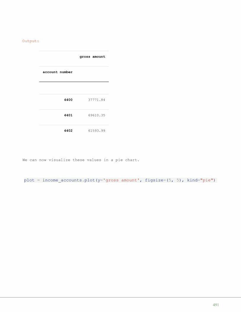
We can now visualize these values in a pie chart.

plot = income_accounts.plot(y='gross amount', figsize=(5, 5), kind="pie")

Output:

gross amount

account number

4400 37771.84

4401 69610.35

4402 61593.99

491

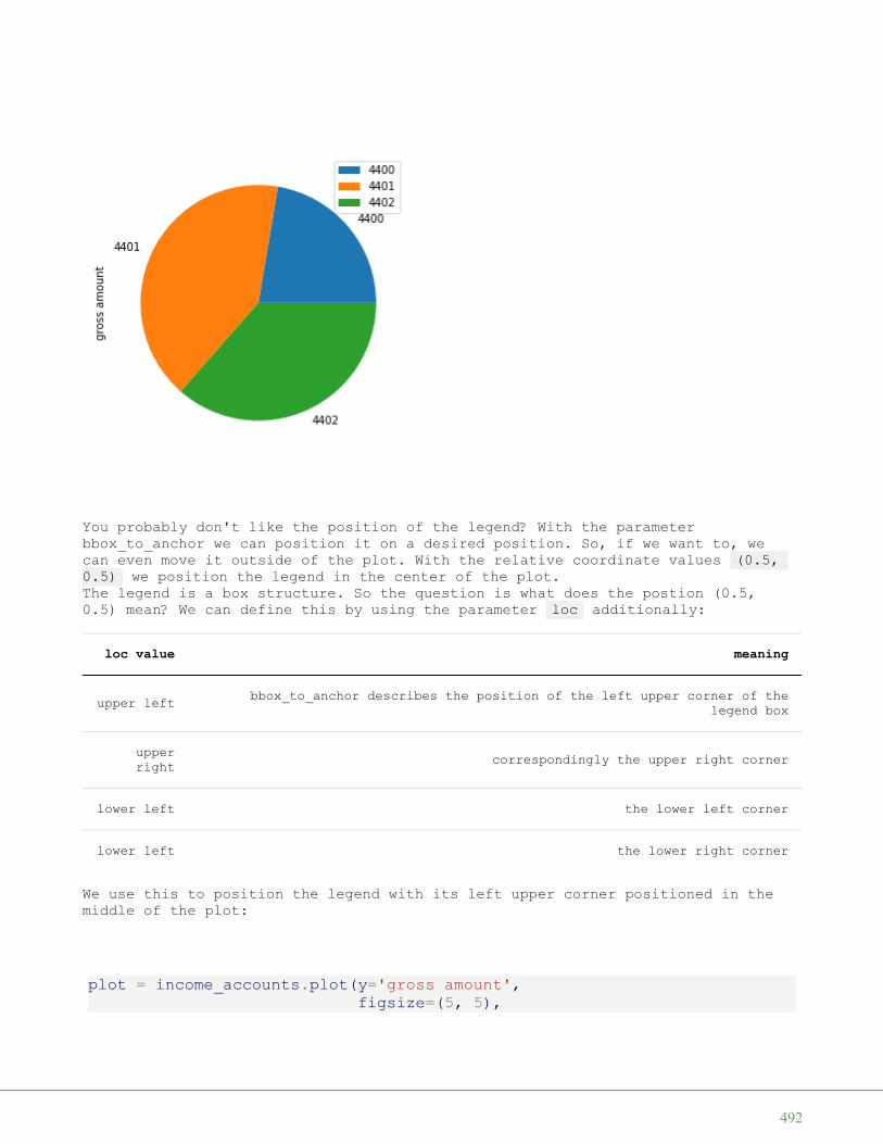
You probably don't like the position of the legend? With the parameterbbox_to_anchor we can position it on a desired position. So, if we want to, wecan even move it outside of the plot. With the relative coordinate values (0.5,0.5) we position the legend in the center of the plot.The legend is a box structure. So the question is what does the postion (0.5,0.5) mean? We can define this by using the parameter loc additionally:

loc value meaning

upper left bbox_to_anchor describes the position of the left upper corner of thelegend box

upperright correspondingly the upper right corner

lower left the lower left corner

lower left the lower right corner

We use this to position the legend with its left upper corner positioned in themiddle of the plot:

plot = income_accounts.plot(y='gross amount',figsize=(5, 5),

492

kind="pie")plot.legend(bbox_to_anchor=(0.5, 0.5),

loc="upper left")

Now we position the lower right corner of the legend into the center of the plot:

plot = income_accounts.plot(y='gross amount', figsize=(5, 5), kind="pie")plot.legend(bbox_to_anchor=(0.5, 0.5),

loc="lower right")

Output: <matplotlib.legend.Legend at 0x7f172ca03a90>

493

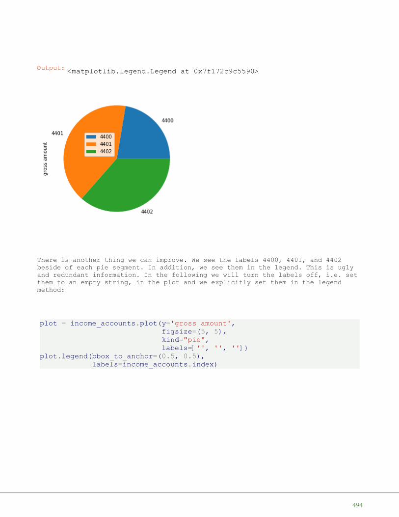
There is another thing we can improve. We see the labels 4400, 4401, and 4402beside of each pie segment. In addition, we see them in the legend. This is uglyand redundant information. In the following we will turn the labels off, i.e. setthem to an empty string, in the plot and we explicitly set them in the legendmethod:

plot = income_accounts.plot(y='gross amount',figsize=(5, 5),kind="pie",labels=['', '', ''])

plot.legend(bbox_to_anchor=(0.5, 0.5),labels=income_accounts.index)

Output: <matplotlib.legend.Legend at 0x7f172c9c5590>

494

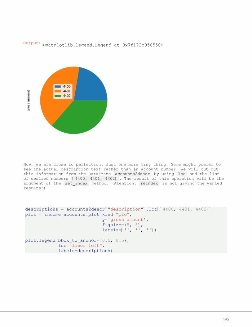
Now, we are close to perfection. Just one more tiny thing. Some might prefer tosee the actual description text rather than an account number. We will cut outthis information from the DataFrame accounts2descr by using loc and the listof desired numbers [4400, 4401, 4402] . The result of this operation will be theargument of the set_index method. (Atention: reindex is not giving the wantedresults!)

descriptions = accounts2descr["description"].loc[[4400, 4401, 4402]]plot = income_accounts.plot(kind="pie",

y='gross amount',figsize=(5, 5),labels=['', '', ''])

plot.legend(bbox_to_anchor=(0.5, 0.5),loc="lower left",labels=descriptions)

Output: <matplotlib.legend.Legend at 0x7f172c956550>

495

Would you prefer a bar chart? No problem, we just have to set the parameterkind to bar instead of pie :

plot = income_accounts.plot(y='gross amount',figsize=(5, 5),kind="bar",legend=False)

Output: <matplotlib.legend.Legend at 0x7f172c8ba8d0>

496

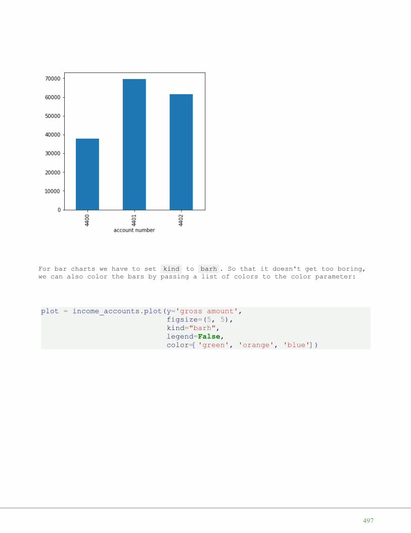
For bar charts we have to set kind to barh . So that it doesn't get too boring,we can also color the bars by passing a list of colors to the color parameter:

plot = income_accounts.plot(y='gross amount',figsize=(5, 5),kind="barh",legend=False,color=['green', 'orange', 'blue'])

497

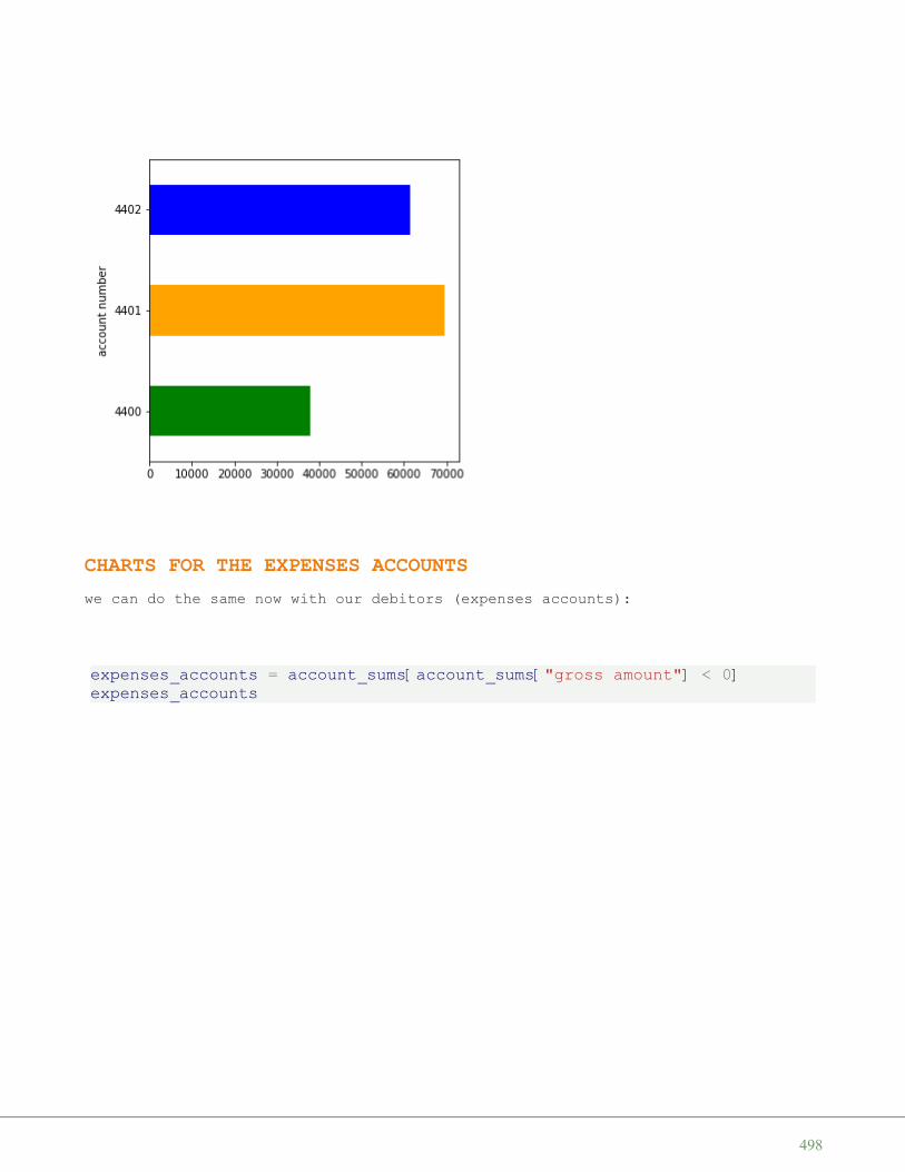
CHARTS FOR THE EXPENSES ACCOUNTSwe can do the same now with our debitors (expenses accounts):

expenses_accounts = account_sums[account_sums["gross amount"] < 0]expenses_accounts

498

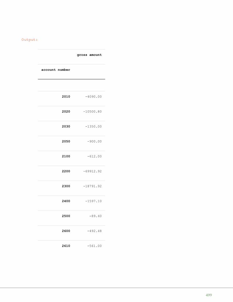
Output:

gross amount

account number

2010 -4090.00

2020 -10500.80

2030 -1350.00

2050 -900.00

2100 -612.00

2200 -69912.92

2300 -18791.92

2400 -1597.10

2500 -89.40

2600 -492.48

2610 -561.00

499

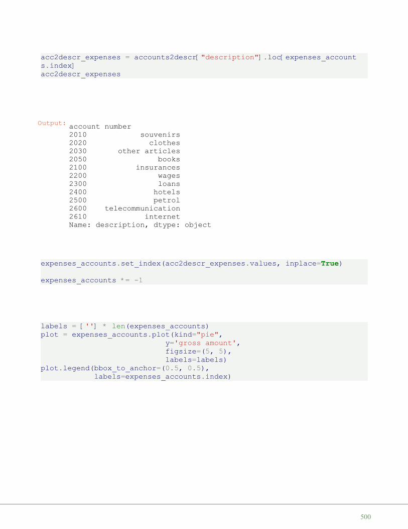
acc2descr_expenses = accounts2descr["description"].loc[expenses_accounts.index]acc2descr_expenses

expenses_accounts.set_index(acc2descr_expenses.values, inplace=True)expenses_accounts *= -1

labels = [''] * len(expenses_accounts)plot = expenses_accounts.plot(kind="pie",

y='gross amount',figsize=(5, 5),labels=labels)

plot.legend(bbox_to_anchor=(0.5, 0.5),labels=expenses_accounts.index)

Output: account number2010 souvenirs2020 clothes2030 other articles2050 books2100 insurances2200 wages2300 loans2400 hotels2500 petrol2600 telecommunication2610 internetName: description, dtype: object

500

TAX SUMSWe will sum up the amount according to their tax rate.

journal.drop(columns=["account number"])

Output: <matplotlib.legend.Legend at 0x7f172868f0d0>

501

502

Output:

documentnumber description tax

rategrossamount

date

2020-04-02 8983233038 Zurkan, Köln 19 4105.98

2020-04-02 57550799 Birmann, Souvenirs 19 -1890.00

2020-04-02 14989004 wages 0 -17478.23

2020-04-02 12766279 Filling Station, Petrol 19 -89.40

2020-04-02 3733462359 EnergyCom, Hamburg 19 4663.54

... ... ... ... ...

2020-07-25 5204418668 BoKoData, Bodensee,Konstanz 19 3678.38

2020-07-25 85241331 Hotel, Konstanz 7 -583.00

2020-07-27 26865618 Hotel, Franfurt 7 -450.00

2020-07-26 5892708524 Oscar Zopvar KG,Luxemburg 19 2589.80

2020-07-28 1633775505 Oscar Zopvar KG,Luxemburg 19 3578.46

503

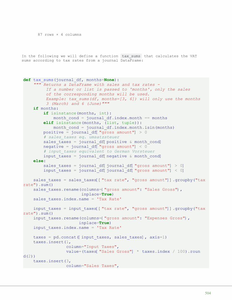
In the following we will define a function tax_sums that calculates the VATsums according to tax rates from a journal DataFrame:

def tax_sums(journal_df, months=None):""" Returns a DataFrame with sales and tax rates -

If a number or list is passed to 'months', only the salesof the corresponding months will be used.Example: tax_sums(df, months=[3, 6]) will only use the months3 (March) and 6 (June)"""

if months:if isinstance(months, int):

month_cond = journal_df.index.month == monthselif isinstance(months, (list, tuple)):

month_cond = journal_df.index.month.isin(months)positive = journal_df["gross amount"] > 0# sales_taxes eq. umsatzsteuersales_taxes = journal_df[positive & month_cond]negative = journal_df["gross amount"] < 0# input_taxes equivalent to German Vorsteuerinput_taxes = journal_df[negative & month_cond]

else:sales_taxes = journal_df[journal_df["gross amount"] > 0]input_taxes = journal_df[journal_df["gross amount"] < 0]

sales_taxes = sales_taxes[["tax rate", "gross amount"]].groupby("taxrate").sum()

sales_taxes.rename(columns={"gross amount": "Sales Gross"},inplace=True)

sales_taxes.index.name = 'Tax Rate'

input_taxes = input_taxes[["tax rate", "gross amount"]].groupby("taxrate").sum()

input_taxes.rename(columns={"gross amount": "Expenses Gross"},inplace=True)

input_taxes.index.name = 'Tax Rate'

taxes = pd.concat([input_taxes, sales_taxes], axis=1)taxes.insert(1,

column="Input Taxes",value=(taxes["Sales Gross"] * taxes.index / 100).roun

d(2))taxes.insert(3,

column="Sales Taxes",

87 rows × 4 columns

504

value=(taxes["Expenses Gross"] * taxes.index / 100).round(2))

return taxes.fillna(0)

tax_sums(journal)

stsum_5 = tax_sums(journal, months=5)stsum_6 = tax_sums(journal, months=6)stsum_5

Output:

Expenses Gross Input Taxes Sales Gross Sales Taxes

Tax Rate

0 -90102.20 0.00 8334.43 -0.00

7 -3847.10 786.85 11240.71 -269.30

19 -14948.32 28386.20 149401.04 -2840.18

505

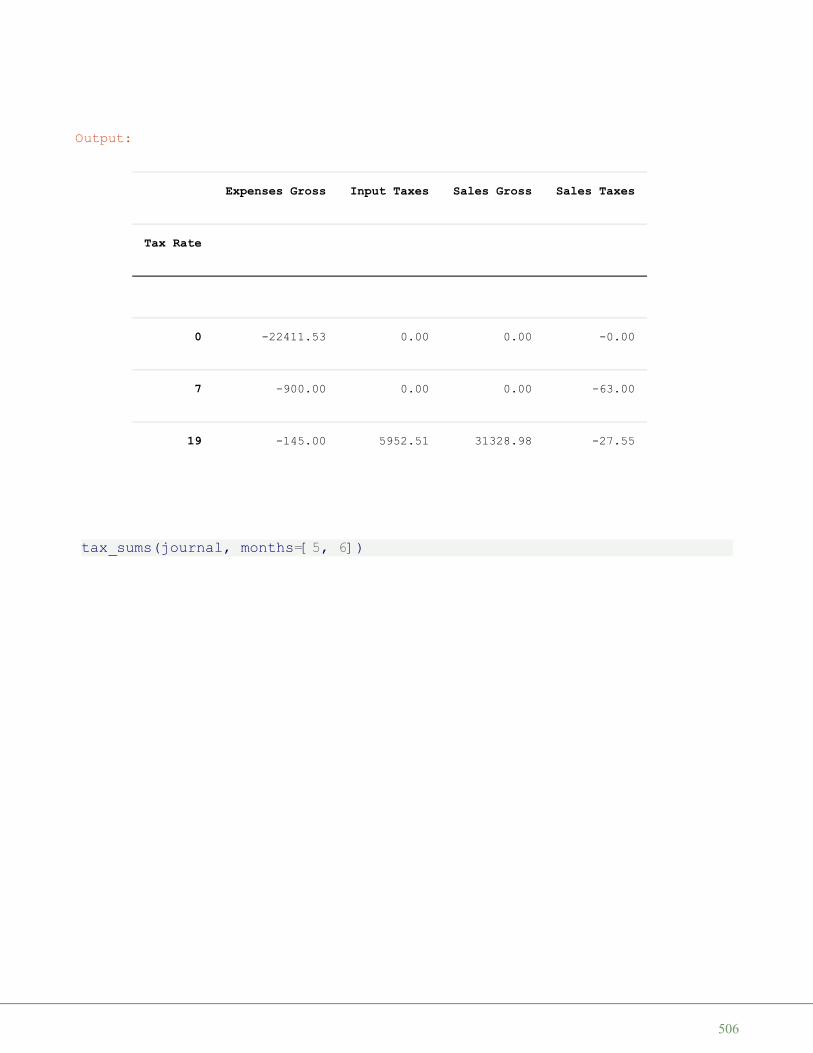
tax_sums(journal, months=[5, 6])

Output:

Expenses Gross Input Taxes Sales Gross Sales Taxes

Tax Rate

0 -22411.53 0.00 0.00 -0.00

7 -900.00 0.00 0.00 -63.00

19 -145.00 5952.51 31328.98 -27.55

506

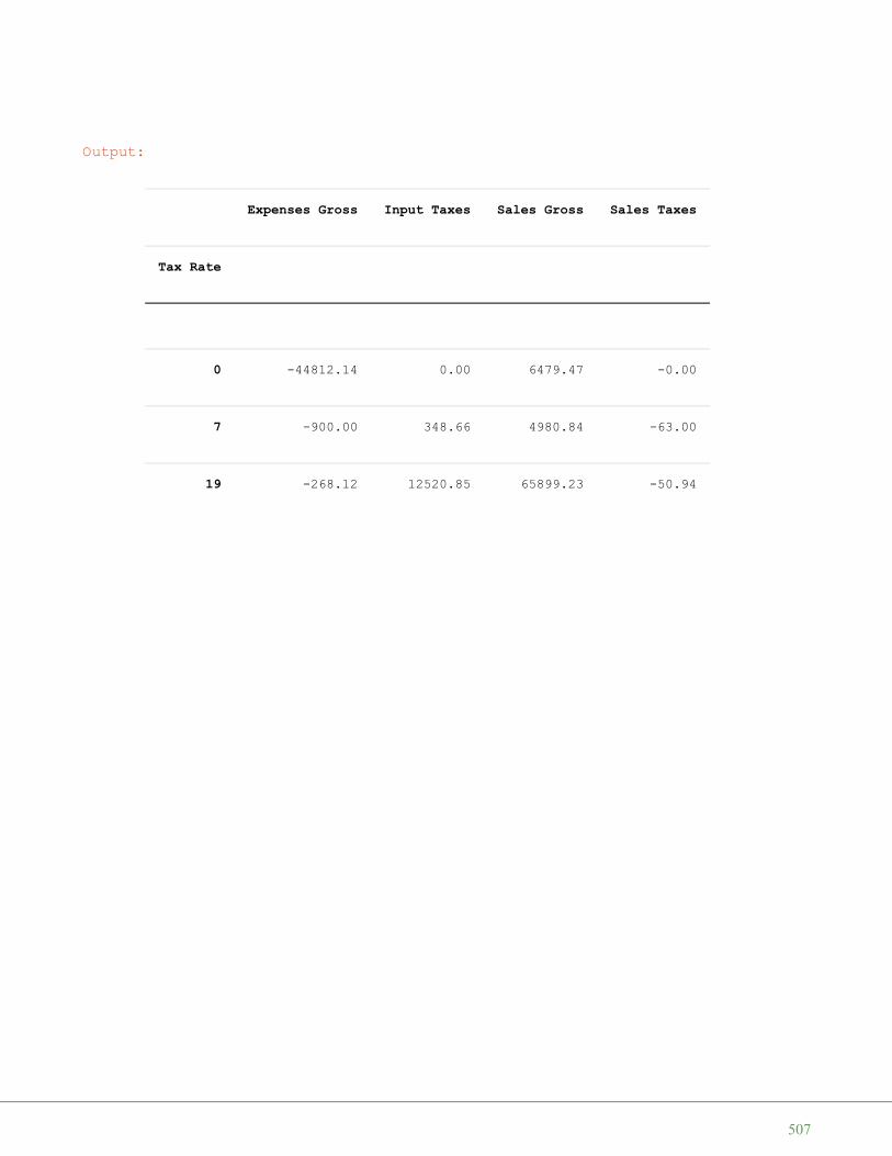
Output:

Expenses Gross Input Taxes Sales Gross Sales Taxes

Tax Rate

0 -44812.14 0.00 6479.47 -0.00

7 -900.00 348.66 4980.84 -63.00

19 -268.12 12520.85 65899.23 -50.94

507

L I N E A R C O M B I N A T I O N

DEFINITIONSA linear combination in mathematics is anexpression constructed from a set of terms bymultiplyingeach term by a constant and adding the results.

Example of a linear combination:

a · x + b · y is a linear combination of x and ywith a and b constants.

Generally;

p = λ1 · x1 + λ2 ·x2 … λn · xn

p is the scalar product of the values x1, x2 … xn and

λ1, λ2 … λn are called scalars.

In most applications x1, x2 … xn are vectors andthe lambdas areintegers or real numbers. (For those, who prefer it mor formally: x1, x2 …xn ∈ V and V is a vector space, and

λ1, λ2 … λn ∈ K with K being a field)

</p>

LINEAR COMBINATIONS IN PYTHONThe vector y = (3.21, 1.77, 3.65) can be easily written as a linear combinationof the unit vectors(0,0,1), (0,1,0) and (1,0,0):

(3.21, 1.77, 3.65) = 3.21 · (1,0,0) + 1.77 (0,1,0) + 3.65 · (0,0,1)

508

We can do the calculation with Python, using the module numpy:

import numpy as npx = np.array([[0, 0, 1],

[0, 1, 0],[1, 0, 0]])

y = ([3.65, 1.55, 3.42])scalars = np.linalg.solve(x, y)scalars

The previous example was very easy, because we could work out the result in ourhead. What about writing our vector y = (3.21, 1.77, 3.65) as a linearcombination of the vectors (0,1,1), (1,1,0) and (1,0,1)? It looks like this inPython:

import numpy as npx = np.array([[0, 1, 1],

[1, 1, 0],[1, 0, 1]])

y = ([3.65, 1.55, 3.42])scalars = np.linalg.solve(x, y)scalars

ANOTHER EXAMPLEAny integer between -40 and 40 can be written as a linear combination of 1, 3, 9,

Output: array([3.42, 1.55, 3.65])

Output: array([0.66, 0.89, 2.76])

509

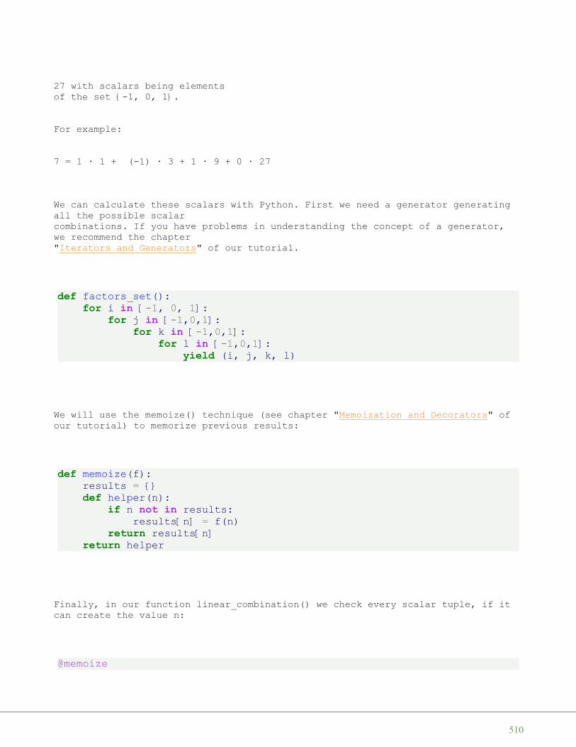
27 with scalars being elementsof the set {-1, 0, 1}.

For example:

7 = 1 · 1 + (-1) · 3 + 1 · 9 + 0 · 27

We can calculate these scalars with Python. First we need a generator generatingall the possible scalarcombinations. If you have problems in understanding the concept of a generator,we recommend the chapter"Iterators and Generators" of our tutorial.

def factors_set():for i in [-1, 0, 1]:

for j in [-1,0,1]:for k in [-1,0,1]:

for l in [-1,0,1]:yield (i, j, k, l)

We will use the memoize() technique (see chapter "Memoization and Decorators" ofour tutorial) to memorize previous results:

def memoize(f):results = {}def helper(n):

if n not in results:results[n] = f(n)

return results[n]return helper

Finally, in our function linear_combination() we check every scalar tuple, if itcan create the value n:

@memoize

510

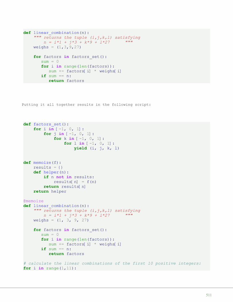
def linear_combination(n):""" returns the tuple (i,j,k,l) satisfying

n = i*1 + j*3 + k*9 + l*27 """weighs = (1,3,9,27)

for factors in factors_set():sum = 0for i in range(len(factors)):

sum += factors[i] * weighs[i]if sum == n:

return factors

Putting it all together results in the following script:

def factors_set():for i in [-1, 0, 1]:

for j in [-1, 0, 1]:for k in [-1, 0, 1]:

for l in [-1, 0, 1]:yield (i, j, k, l)

def memoize(f):results = {}def helper(n):

if n not in results:results[n] = f(n)

return results[n]return helper

@memoizedef linear_combination(n):

""" returns the tuple (i,j,k,l) satisfyingn = i*1 + j*3 + k*9 + l*27 """

weighs = (1, 3, 9, 27)

for factors in factors_set():sum = 0for i in range(len(factors)):

sum += factors[i] * weighs[i]if sum == n:

return factors

# calculate the linear combinations of the first 10 positive integers:for i in range(1,11):

511

print(linear_combination(i))

(1, 0, 0, 0)(-1, 1, 0, 0)(0, 1, 0, 0)(1, 1, 0, 0)(-1, -1, 1, 0)(0, -1, 1, 0)(1, -1, 1, 0)(-1, 0, 1, 0)(0, 0, 1, 0)(1, 0, 1, 0)

512