PNNL-19710

American Recovery and Reinvestment Act (ARRA) Federal Energy Management Program Technical Assistance Project 282

Renewable Energy Opportunities at Fort Gordon, Georgia BK Boyd WJ Gorrissen JR Hand JA Horner AC Orrell BJ Russo MR Weimar JL Williamson RJ Nesse August 2010

DISCLAIMER

This report was prepared as an account of work sponsored by an agency of the United States Government. Neither the United States Government nor any agency thereof, nor Battelle Memorial Institute, nor any of their employees, makes any warranty, express or implied, or assumes any legal liability or responsibility for the accuracy, completeness, or usefulness of any information, apparatus, product, or process disclosed, or represents that its use would not infringe privately owned rights. Reference herein to any specific commercial product, process, or service by trade name, trademark, manufacturer, or otherwise does not necessarily constitute or imply its endorsement, recommendation, or favoring by the United States Government or any agency thereof, or Battelle Memorial Institute. The views and opinions of authors expressed herein do not necessarily state or reflect those of the United States Government or any agency thereof.

PACIFIC NORTHWEST NATIONAL LABORATORY

operated by BATTELLE

for the UNITED STATES DEPARTMENT OF ENERGY

under Contract DE-AC05-76RL01830

Printed in the United States of America

Available to DOE and DOE contractors from the Office of Scientific and Technical Information,

P.O. Box 62, Oak Ridge, TN 37831-0062; Ph: (865) 576-8401 Fax: (865) 576-5728

Email: reports@adonis.osti.gov

Available to the public from the National Technical Information Service, U.S. Department of Commerce, 5285 Port Royal Rd., Springfield, VA 22161

Ph: (800) 553-6847 Fax: (703) 605-6900

Email: orders@ntis.fedworld.gov Online ordering: http://www.ntis.gov/ordering .htm

This document was printed on recycled paper. (9/2003)

PNNL-19710

American Recovery and Reinvestment Act (ARRA) Federal Energy Management Program Technical Assistance Project 282 Renewable Energy Opportunities at Fort Gordon, Georgia BK Boyd WJ Gorrissen JR Hand JA Horner AC Orrell BJ Russo MR Weimar JL Williamson RJ Nesse August 2010 Prepared for U.S. Department of Energy Federal Energy Management Program and the U.S. Army Installation Management Command, Southeast Region under Contract DE-AC05-76RL01830 Pacific Northwest National Laboratory Richland, Washington 99352

iii

Executive Summary

This document provides an overview of renewable resource potential at Fort Gordon, based primarily upon analysis of secondary data sources supplemented with limited on-site evaluations. This effort focuses on grid-connected generation of electricity from renewable energy sources and also on ground source heat pumps for heating and cooling buildings. The effort was funded by the American Recovery and Reinvestment Act (ARRA) as follow-on to the 2005 Department of Defense (DoD) Renewables Assessment. The site visit to Fort Gordon took place on March 9, 2010.

At this time, there are renewable technologies that show economic potential at Fort Gordon. Project feasibility is based on installation-specific resource availability and energy costs and projections based on accepted life-cycle cost methods (Appendix A). The most promising opportunities are ground source heat pumps and a waste-to-energy plant using regional municipal solid waste.

Ground Source Heat Pumps Ground source heat pumps (GSHPs) were evaluated using the data from the 2005 Facility Energy Decision System (FEDS) assessment for Fort Gordon. Open-loop, horizontal closed-loop, and vertical closed-loop configurations were analyzed for all buildings included in that assessment. Simple paybacks range from 4.1 to 26.2 years (for results with savings-to-investment ratios greater than 1.0), depending on the building type and technology evaluated. Ground source heat pumps should also always be considered for new construction, which is typically more economic than retrofit applications. Detailed ground source heat pump results are provided in Appendix D.

Waste-to-Energy There is sufficient municipal solid waste in the area to build an economic waste-to-energy plant at Fort Gordon. There are four landfills within 60 miles of Fort Gordon that collect nearly 657,000 tons per year, which is expected to remain constant in the future. Some of this waste could be available for energy generation, with savings-to-investment ratios ranging from 1.6 to 1.7, and internal rates of return (IRR) ranging from 10% to nearly 13%, depending on the size of the plant and technology used (e.g., combustion or gasification). Further details can be found in Appendix B.

Other Renewable Resources Other renewable technologies did not prove to be cost-effective under current conditions and assumptions. Other biomass resources (including crop residues, animal waste, dedicated crops, regional wood waste, mill residue, landfill gas, and wastewater treatment plant sludge) were found to be too scarce in the Fort Gordon area or too expensive to transport to consider a generation project (Appendix B). Geothermal power generation requiring new wells to be drilled was found to be a poor economic option as well (Appendix C). Solar projects are not likely to be cost-effective in the near future either, requiring an electricity cost of about 28¢/kWh to generate a 10% IRR (Appendix E). Lastly, the wind resource at Fort Gordon is insufficient for an

iv

economic wind project (Appendix F). With the average wind speed of 4.1 m/s, electricity would need to cost 57¢/kWh to obtain a 10% internal rate of return.

Renewable resources with promising economic potential are summarized in Table 1. The impact of ground source heat pumps depends on the extent of technology deployment. Many building groups were found to be promising candidates for retrofits, particularly those using fuel oil and propane. There were several buildings consuming natural gas that were found to be good candidates, and new construction and locations with failed heating and cooling equipment, or buildings undergoing major renovations should be considerations, as well. Additionally, if Fort Gordon were to develop a waste-to-energy project with site waste combined with all wastes going to Augusta-Richmond County Landfill, it could provide about 377 GWh of electricity, or 191% of the FY 2009 electrical consumption at Fort Gordon.

Increasing use of renewable energy makes sense for the Army. The goal of this report is to help Army personnel make sense of renewable energy opportunities at Fort Gordon.

Table 1: Summary of Promising Renewable Energy Projects at Fort Gordon

RenewableResource and

Technology

ResourceEstimate

Earliest Output Figures of Merit

FinancingMechanisms

Evaluated

Location--Requirements Key Assumptions Next Steps

Comments

Ground Source Heat Pump

(Thermal Energy)

To be determined.

2011

ECIP scenario: 5-26 year payback

UESC/ESPC scenario: 6-20 year

payback

ECIPUESC/ESPC

Space near building for heat exchange

wells or loop.

Soil data from 2007 study of Brems Barracks is sufficient to provide a preliminary screening.

Pursue retrofits in buildings that were found

to be economically feasible; focus initially on buildings served by fuel oil and propane. Secure funding to add GSHPs to

new construction.

Municipal Waste-to-Energy Plant

using Combustion or Gasification Technologies

31 - 51 MW(using Gordon,

Augusta-Richmond, or Three Rivers Landfill MSW)

2013

ECIP scenario: 1.6-1.7 SIR, 8.2-9.0 year

payback at 5.5¢/kWh

IPP scenario: 10.6-12.7% IRR at

5.5¢/kWh

(function of technology and

plant size)

ECIPIPP

A 5-acre site near major roads, a utility substation, water, sewage, and an

appropriate industrial infrastructure, plus feedstock storage

space.

MSW available for WTE plant, and can be brought

on site.

Plant location can be secured on Fort Gordon.

Tipping fees of $30-35/ton available with MSW delivery to plant.

Confirm waste availability and tipping fees.

Economics are highly dependent upon tipping fee available from waste

providers.

Goo

d Po

tent

ial

defin

itely

wor

th p

ursu

ing

SIR = savings-to-investment ratio ECIP = Energy Conservation Investment Program IPP = independent power producer UESC = Utility Energy Services Contract ESPC = Energy Savings Performance Contract MSW = municipal solid waste WTE = waste-to-energy

Greenhouse Gas Emissions The emissions from a waste-to-energy plant will depend on the type of plant selected and will offset electricity purchased from Georgia Power. A DOD-owned WTE combustion plant located on Fort Gordon would contribute about 0.54 kg net CO2 equivalent per kWh generated. A DOD-owned WTE gasification plant located on Fort Gordon would contribute about 0.17 kg net CO2 equivalent per kWh generated.

v

Emission reductions from GSHPs are typically achieved by replacing a fossil fuel heating source with electricity and providing a more efficient heating and cooling system, and vary depending on the loads in the building, the fuel replaced, and the type of heat pump system installed. If all cost-effective open-loop projects were implemented, the total CO2 savings would be approximately 5,705 tons per year. Likewise, if only cost-effective vertical closed-loop systems were pursued, the total CO2 savings would be approximately 341 tons per year. In reality, Fort Gordon will likely implement a mix of GSHP configurations, and a portion of potential projects will not be feasible because of land use or groundwater restrictions.

vi

vii

Table of Contents

Executive Summary ......................................................................................................................................... iii

Ground Source Heat Pumps ............................................................................................................... iii

Waste-to-Energy ................................................................................................................................. iii

Other Renewable Resources .............................................................................................................. iii

Introduction....................................................................................................................................................... 1

Overview of Federal and DoD Renewable Requirements ............................................................................... 3

Analysis of Renewables at Fort Gordon .......................................................................................................... 5

Approach for Identifying, Analyzing, and Implementing Renewable Energy Projects ........................ 5

Importance of Financing Mechanisms for Project Feasibility ............................................................. 6

The Political and Economic Environment for Renewables at Fort Gordon ......................................... 7

Fort Gordon Energy Characterization .................................................................................... 7

State Incentives for Renewable Project Development ........................................................... 7

Federal Incentives for Renewable Project Development ....................................................... 8

Results and Recommendations ....................................................................................................................... 9

Ground Source Heat Pump Findings and Recommendations ............................................................ 9

Waste-to-Energy Findings and Recommendations .......................................................................... 11

Biomass Findings and Recommendations ....................................................................................... 12

Solar Energy Findings and Recommendations ................................................................................ 12

Wind Energy Findings and Recommendations ................................................................................. 13

Geothermal Power Plant Findings and Recommendations .............................................................. 13

Main Report Sources of Information ................................................................................................. 15

Appendix A: Business Case Analysis Approach .......................................................................................... A-1

Appendix B: Analysis of Biomass and Waste-to-Energy Opportunities ....................................................... B-1

Appendix C: Analysis of Geothermal Power Plant Opportunities ................................................................ C-1

Appendix D: Analysis of Ground Source Heat Pump Opportunities ............................................................ D-1

Appendix E: Analysis of Solar Opportunities ................................................................................................ E-1

Appendix F: Analysis of Wind Opportunities ................................................................................................ F-1

viii

Figures

Figure A-1: FATE2-P Methodology ........................................................................................................... A-5 Figure C-1: Estimated temperature at 4 km depth for Eastern United States .......................................... C-3 Figure E-1: Dual-Axis Tracking PV Array .................................................................................................. E-1 Figure E-2: Integrated PV on Rooftop ....................................................................................................... E-2 Figure E-3: Fort Huachuca Stirling Engine Solar Dish .............................................................................. E-2 Figure E-4: Solar Insolation Levels (NREL 2008) ..................................................................................... E-4 Figure E-5: Average Daily Insolation at Fort Gordon ................................................................................ E-6

Tables

Table 1: Summary of Promising Renewable Energy Projects at Fort Gordon ........................................... iv Table 2: Legislated Renewable Energy Targets for DoD ............................................................................ 3 Table 3: Summary of Fort Gordon Renewable Energy Opportunities ......................................................... 9 Table 4: Simple Payback Period for Building Groups Analyzed in FEDS for GSHPs* .............................. 10 Table 5: Waste near Fort Gordon .............................................................................................................. 11 Table 6: Fort Gordon WTE Results ............................................................................................................ 12 Table 7: Economic Results for Solar Technologies at Fort Gordon........................................................... 13 Table 8: Economic Assessment of Wind Power ........................................................................................ 13 Table 9: Geothermal Performance, Cost, and Economic Characteristics .................................................. 14 Table 10. Emissions Reduction from Proposed GSHP Projects. ............................................................... 14 Table A-1: Renewable Electricity Generation Tax Credits ....................................................................... A-3 Table A-2: MACRS Depreciation Rates for Renewable Energy Projects ................................................ A-3 Table A-3: Discount Rate Assumptions in the ECIP Model ..................................................................... A-4 Table B-1: Crops and Biomass Production near Fort Gordon ................................................................. B-5 Table B-2: Waste near Fort Gordon ......................................................................................................... B-8 Table B-3: Economic Assumptions, constant $2009 ............................................................................. B-10 Table B-4: Fort Gordon WTE Results .................................................................................................... B-11 Table C-1: Geothermal Performance, Cost, and Economic Characteristics ............................................ C-4 Table D-1: Building Groups Analyzed in FEDS for GSHPs ..................................................................... D-2 Table D-2: Buildings Analyzed in FEDS for GSHPs* ............................................................................... D-4 Table D-3: Simple Payback Period for Building Groups Analyzed in FEDS for GSHPs* ........................ D-8 Table D-4: Detailed GSHP Economic Results ......................................................................................... D-9 Table E-1: Monthly Averaged Insolation Incident on a South-facing Tilted Surface at Fort Gordon (kWh/m2/day) ............................................................................................................................................. E-5 Table E-2: Roof-Integrated Membrane PV Analysis at Fort Gordon ....................................................... E-8 Table E-3: Solar Electric Production by System Type at Fort Gordon .................................................... E-8 Table E-4: Monthly Average RTP Charges for Solar ............................................................................... E-9 Table E-5: Economic Results for Solar Technologies at Fort Gordon ................................................... E-10 Table F-1: Classes of Wind Power Density at 50 Meters .......................................................................... F-3 Table F-2: Summary of Wind Resource Data ........................................................................................... F-4 Table F-3: Performance, Cost, and Economic Characteristics ................................................................. F-5 Table F-4: Economic Assessment of Wind Power .................................................................................... F-5

1

Introduction

On Feb. 13, 2009, Congress passed the American Recovery and Reinvestment Act (ARRA) of 2009 at the urging of President Obama, who signed it into law 4 days later. A direct response to the economic crisis, the Recovery Act has three immediate goals:

• Create new jobs and save existing ones • Spur economic activity and invest in long-term growth • Foster unprecedented levels of accountability and transparency in government spending1

Pacific Northwest National Laboratory (PNNL) has been directed to conduct detailed analyses of the potential for electricity generation at selected U.S. Army installations, in accordance with similar analysis performed for the U.S. Army Installation Management Command (IMCOM). To be comparable in scope, this study used the same approach as the studies conducted under IMCOM funding. The goal of the analyses is to identify economically feasible opportunities for generation of electricity from renewable resources—generation that is significant enough to warrant connection to the grid and/or to contribute in a meaningful way to the aggressive renewable energy goals of the Army and the Department of Defense (DoD).

.

In 2005, PNNL led a study to identify utility-scale electricity generation opportunities at DoD installations. That study focused on solar, wind, and geothermal. A limited number of attractive large-scale commercial opportunities were identified, and their implementation is now being pursued. The study also identified a number of potential smaller opportunities that needed to be investigated further before project implementation decisions could be made.

This analysis of opportunities at Fort Gordon is one of the suite of analyses being conducted at Army installations as follow-on to the 2005 study. The goal is to revisit potential renewable opportunities, updating the analysis for changes in economics, incentives, knowledge about the available renewable resource, and other factors. It is focused on any size project greater than 1 MW. In addition, PNNL evaluated the potential for biomass, waste-to-energy, and retrofitting heating and cooling systems in existing buildings with ground source heat pumps (GSHPs). Retrofitting with GSHPs is obviously not an electricity generation opportunity, but it is an opportunity for significant energy savings and replacement of fossil fuels across DoD, and can contribute toward some renewable goals. As part of the analysis, PNNL was directed to lay out the steps necessary to implement the project opportunities that are identified.

The overall findings of this analysis are summarized in the main body of the report. The business case approach that underlies the analysis of each renewable technology is documented in Appendix A. Appendix B describes the analysis conducted on biomass and waste-to-energy technologies. Appendix C describes the geothermal analysis; Appendix D, the GSHP analysis; Appendix E, the solar analysis; and Appendix F, the wind energy analysis.

1 http://www.recovery.gov/

2

3

Overview of Federal and DoD Renewable Requirements

The Army needs to satisfy multiple goals and constraints while securing its energy supplies—focusing on procurement of the lowest-cost energy that meets high reliability standards and minimum vulnerability to interruption from natural or intentional causes. Overlaid on this challenge is the need to comply with a series of somewhat contradictory statutes and policies, as laid out in Table 2. These include:

• Energy Policy Act (EPAct) Section 203

•

. This law mandates the minimum contribution of renewable electricity to an installation’s total electricity consumption. The target fractions are 3% for FY 2007 through FY 2009, 5% through FY 2012, and not less than 7.5% beginning in FY 2013.

Executive Order (EO) 13423

•

. The Executive Order reiterates the EPAct goals; however, it uses a different basis than EPAct for measuring and crediting progress. For example, renewable thermal energy counts toward the renewable goal.

National Defense Authorization Act (NDAA)

•

. The NDAA codifies DoD’s voluntary goal of 25% by 2025, but does not include any interim targets. Renewable thermal energy counts toward the renewable goal.

Energy Independence and Security Act (EISA)

. EISA established two additional renewable goals for new buildings and retrofits. One requires 30% of domestic hot water to be supplied from solar energy, and the other requires all fossil fuels used in buildings to be displaced by 2030. This is not a power generation goal like the others, but is important to note.

Table 2: Legislated Renewable Energy Targets for DoD

EPAct Section 203

Executive Order 13423

National Defense Authorization

Act

Energy Independence

and Security Act

Target / Goal

Increasing targets reaching 7.5% of electric energy

from renewables

7.5% of electric energy from

renewables; 50% from new (post-1998)

sources

Equivalent of 25% of electric energy from renewables

30% of hot water demand from

solar

Target Dates 2013 2013 2025 All new

construction / major renovations

Mandatory? Yes Yes No Yes

Considers thermal energy “renewable”? No Yes Yes N/A

This assessment is primarily for renewable energy provision and retrofit applications in existing buildings. Accordingly, potential in new building construction is mentioned only in passing. The Department of Energy (DOE) is responsible for developing guidance for EPAct and EO 13423. DOE’s guidelines for EO compliance, unlike EPAct, allow credit for renewable energy

4

that reduces electricity use from thermal sources; however, it adds a requirement that at least 50% of renewable energy must come from “new” resources: those put into service after January 1, 1999.

Congress did not provide a definition of “renewable” in the NDAA language, and DOE is not responsible for establishing DoD or Army policies to achieve the goals in the NDAA. The current Army energy strategy and associated draft renewable policy takes an expansive view of renewables that encompasses thermal energy from renewable sources. As a result, the Army needs to proceed in a way that makes sense for the Army in a good faith effort to satisfy Congressional, Administration, and Pentagon mandates and directives. The expectation is that the Army will meet the stricter definitions of EPAct on its way to meeting the much higher renewable goals of the NDAA.

5

Analysis of Renewables at Fort Gordon

PNNL’s renewable energy analysis includes a preliminary assessment based on readily available resources, a site visit to present the preliminary findings and gather additional information, and a concluding assessment, which is documented in this report.

The site visit to Fort Gordon took place on March 9, 2010 with Ron Nesse and Brian Boyd attending for PNNL. Fort Gordon personnel at the briefing included Bonnie Terrill (Energy Engineer), Jim Sloan (Environmental Division), Steve Willard (Environmental Director), Michael Sarber (Director MWR), and Glenn Stubblefield (Operations & Maintenance Manager). Separate discussions were held with Kathy Riley (Environmental Protection Specialist) and John Wellborn (Compliance Branch Chief) during the site visit, and subsequent information was provided by Allen Braswell (Installation Forester and Wildlife Fire Program Manager).

Approach for Identifying, Analyzing, and Implementing Renewable Energy Projects Renewable energy resources are unlike conventional resources because the “fuel” is essentially free. However, harnessing this free resource requires substantial investment in resource exploration, characterization, and collection; project development; and ongoing maintenance and operation. A renewable resource is like purchasing a new car with a lifetime of fuel as part of the purchase agreement. First costs are much higher, but total cost may be (should be) lower over the long run.

Economic development of renewable energy depends upon:

• Access to a renewable resource,

• Development costs, and

• Financing that is economically attractive and allowed by Federal and DoD regulations.

Each of these is critically important.

Obviously, a renewable resource has to be available and accessible to be developed. The best resources are those with the greatest potential for displacing conventional fuels or power supplies. Development cost, however, is the great equalizer, and a project based upon an excellent resource that is located many miles away may be inferior to a project based upon a lesser resource nearby. For example, an excellent wind resource far from an adequate transmission line may be less attractive than an inferior resource adjacent to a transmission line. Similarly, waste resources that could be used in a central plant may not be economic, even if they are “free,” if the transportation, handling, and storage costs are greater than the cost of continued use of conventional heating fuels.

Development costs are relatively comparable for similar size projects, irrespective of resource quality. This is why the quality of the resource is so important—namely for the same investment, you get more out of a high quality resource than a lower quality one. But, development costs also include access to transmission capacity for shipping power to users, or alternatively, access to a retail customer. This is a critical difference, because power shipped

6

over transmission lines has to compete against the prevailing wholesale price for power from conventional resources. Typically, renewables are not competitive in these markets, unless a buyer specifically demands renewable power. On the other hand, if the power can be used on site to displace power purchased from the local utility, it competes against that customer’s retail power price or utility rate. Because retail power prices include costs for transmission, distribution, and administrative costs, they are higher than wholesale power prices and make competing renewable projects more attractive economically.

It is important that economic analyses of renewable energy opportunities use realistic data on avoided energy costs, project costs, and available incentive funds, if any. A common analytic mistake is the use of average cost per kWh—the so-called “blended” rate. Using the blended rate will lead to inaccurate results when the renewable resource is intermittent (like wind and solar) because intermittent resources cannot be guaranteed to reduce peak demand. Even non-intermittent resources may not result in reduced peak demand because of periodic maintenance shutdowns and unscheduled outages. The economic analyses in this report use only the energy component of the power bill to evaluate intermittent resources, which is admittedly conservative. The blended rate is used for economic analysis of base-load resources.

Additionally, the installation’s utility may impose a standby or other fee in the face of a major on-site generation project that needs to be reflected in the project’s cost calculation. The analyses conducted here make no assumptions regarding standby charges, because those are typically assessed on a project-by-project basis.

The economic analyses in this report used two perspectives: Energy Conservation Investment Program (ECIP) funding and third-party financing. Under the latter arrangement, power is sold from large generation projects through a contract that is commonly called a power purchase agreement or PPA. This analysis assumed an internal rate of return (IRR) of 10% is the minimum required to attract a developer. GSHPs can be third-party financed through utility energy services contracts (UESCs) or energy savings performance contracts (ESPCs). These are implemented by a third party but result in government ownership. The ECIP analyses assumed projects were not cost-effective if the savings-to-investment ratio (SIR) was less than 1.0. These two options are the lowest-cost among all the options typically available to Army customers.

Importance of Financing Mechanisms for Project Feasibility Financing is a critical determinant of development costs because the high first costs are sensitive to financial factors such as incentive payments, tax breaks, and interest rates. Incentive payments and tax breaks reduce first costs, lowering both the overall project cost and interest costs. Because financing is so critical, project economics (payback rates, life-cycle costs, etc.) constitute the best initial screen for project potential. That screen needs to reflect various financing alternatives, which in turn, helps energy managers decide on the best project development approach.

This study focuses on “utility-scale” projects on the premise that if a good renewable resource exists at a site, it should be developed to its maximum potential. Projects smaller than 1 MW are not analyzed because of their small contribution to renewable goals and their poor economics compared to larger projects. These large projects typically exceed any realistic expectation for

7

appropriated funding, and so the assessments focus on commercial (third-party) development of projects. Besides funding limitations, there are other reasons that these large projects should be implemented by third-party investors—under current DoD philosophy, resource development is not a core DoD mission and should be left to the private sector. In addition, private developers can take advantage of tax credits and they value renewable energy credits (RECs) more highly than the Army does. As a result, letting the developers claim tax credits and retain RECs, if available, will reduce the cost of energy to the installation if the developer is selling power from the project to the site.

The Political and Economic Environment for Renewables at Fort Gordon Fort Gordon Energy Characterization

Fort Gordon is provided electricity by Georgia Power. The site consumed a total of 197,579 MWh (23 MWaverage) in FY09. Fort Gordon is a summer-peaking facility, with a 2009 peak consumption of 18,533 MWh in July, and a 2009 peak demand of about 33 MWpeak

Georgia Power charges Fort Gordon for electricity through the real time pricing hour ahead (RTP-HA-2) rate schedule. Real time pricing schedules have variable rates for each hour of each day. Between FY07 through FY09, the electric rate at Fort Gordon varied from 1.72¢/kWh to 36.96¢/kWh. Because real time pricing rates can be relatively volatile compared to fixed-rate schedules, the rate analysis examined rates for FY07 through FY09. Over this range, the average value of electricity purchased by Fort Gordon was about 5.5¢/kWh, and there is no demand charge. This average value was used for base-load renewable energy resources, which are not intermittent. These resources include biomass, waste-to-energy, and geothermal.

in August. The total electricity bill in FY09 was $12.9 million.

Solar and wind are intermittent resources, and the output profile for systems that harvest these resources may not match Fort Gordon’s energy demand profile. Consequently, wind was assumed to displace energy valued at 4.76¢/kWh, which is the site’s simple average electric rate over FY07 through FY09. Solar systems naturally produce more energy during the summer and daytime periods than in the winter or at dusk and night. Consequently, solar energy was assumed to displace energy ranging in value from 5.84¢/kWh to 6.05¢/kWh depending on the technology considered. For additional detail regarding the value of energy for solar renewable systems, see Appendix E.

State Incentives for Renewable Project Development

State incentives for renewable energy in Georgia include a Clean Energy Tax Credit, a potential production incentive from Georgia Power, a sales tax exemption for biomass and a net metering rule limited to 100 kW (DSIRE 2010). Thus, on-site distributed power cannot be sized much larger than the fort requires. The biomass sales tax exemption was the most valuable for the renewable energy resources in this study. The Clean Energy Tax Credit provides a 35% investment tax credit for solar photovoltaic (PV), wind, and biomass. The credit is limited to $500,000. For modeling purposes, PNNL calculated the percentage of the limit for each technology and applied it as the amount of energy tax credit. Thus, a $4,000/kW PV system would receive a 12.5% investment tax credit.

8

Georgia Power offers a $0.1831/kWh production incentive to anyone selling solar power to the utility. The language indicated that the power actually had to be sold to Georgia Power so PNNL did not include the incentive. Biomass receives a 100% exemption from Georgia’s sales tax. The exemption amounts to a 7% reduction in costs for biomass projects. The exemption does not apply to municipal solid waste. Georgia’s net metering rule is limited to 100 kW. Thus, on-site distributed power cannot be sized much larger than the fort requires. A sales tax of 7% (GDOR 2009b) was applied where appropriate in this analysis. State corporate income taxes of 6% were applied (GDOR 2010). A property tax rate of 1.2% was assumed. Georgia’s property tax assessment is 40 % of fair market value. (GDOR 2009a).

Federal Incentives for Renewable Project Development

Federal incentives for renewable energy include investment tax credits for corporations, significantly accelerated depreciation of equipment, and production tax credits. A 30% tax credit is available for PV projects, and 10% for geothermal and biomass electricity projects, with no incentive limits. The credits may be taken on equipment placed in service prior to January 1, 2017. Wind is not eligible for the business energy tax credit. The tax basis for depreciation must be reduced by the amount of any Federal subsidy used in the financing of the eligible equipment.

Depreciation for most renewable energy equipment qualifies for significantly accelerated depreciation. For solar, wind, and geothermal, the modified accelerated cost recovery system (MACRS) provides for 5-year recovery of the cost of equipment. The 5-year recovery period does not apply to biomass or WTE equipment.

The renewable energy production tax credit (PTC), originally established in 1992, and provides a tax credit for each kilowatt-hour of electricity produced. The PTC is 2.1¢/kWh for wind, geothermal, and closed-loop biomass (biomass that is grown with the sole purpose of being used to generate energy), and can be taken for 10 years. The PTC is 1.1¢/kWh for electricity produced from open-loop biomass and municipal solid waste resources, and can be taken for 5 years. Solar electricity generation has been excluded for equipment placed in service after December 2005. The PTC has been allowed to lapse and has then been renewed several times.

Available tax incentives reduce the first-year costs of qualified renewable projects. The lower first cost also reduces the amount of money that must be borrowed to develop a project and thus, the associated interest and carrying costs. The combination reduces the delivered cost of power if developed by a private party with a tax obligation. Government-owned projects do not benefit from tax-based incentives. All of the PPA analyses conducted in this report assume that the PTC and other tax credits will be available when the equipment is placed in service.

9

Results and Recommendations

A summary of analysis results is presented in Table 3, broken down into economic (green) or uneconomic (red) projects. The underlying analyses and recommendations for each of these technologies and potential projects are provided in the following subsections.

Table 3: Summary of Fort Gordon Renewable Energy Opportunities Renewable

Resource andTechnology

ResourceEstimate

Earliest Output Figures of Merit

FinancingMechanisms

Evaluated

Location--Requirements Key Assumptions Next Steps

Comments

Ground Source Heat Pump

(Thermal Energy)

To be determined.

2011

ECIP scenario: 5-26 year payback

UESC/ESPC scenario: 6-20 year

payback

ECIPUESC/ESPC

Space near building for heat exchange

wells or loop.

Soil data from 2007 study of Brems Barracks is sufficient to provide a preliminary screening.

Pursue retrofits in buildings that were found

to be economically feasible; focus initially on buildings served by fuel oil and propane. Secure funding to add GSHPs to

new construction.

Municipal Waste-to-Energy Plant

using Combustion or Gasification Technologies

31 - 51 MW(using Gordon,

Augusta-Richmond, or Three Rivers Landfill MSW)

2013

ECIP scenario: 1.6-1.7 SIR, 8.2-9.0 year

payback at 5.5¢/kWh

IPP scenario: 10.6-12.7% IRR at

5.5¢/kWh

(function of technology and

plant size)

ECIPIPP

A 5-acre site near major roads, a utility substation, water, sewage, and an

appropriate industrial infrastructure, plus feedstock storage

space.

MSW available for WTE plant, and can be brought

on site.

Plant location can be secured on Fort Gordon.

Tipping fees of $30-35/ton available with MSW delivery to plant.

Confirm waste availability and tipping fees.

Economics are highly dependent upon tipping fee available from waste

providers.

Cellulosic Biomass Energy

Plant36 MW 2013

8.42¢/kWh projected electric generation rate

IPP

A 5-acre site near major roads, a utility substation, water, sewage, and an

appropriate industrial infrastructure, plus feedstock storage

space.

Regional wood waste is unavailable at present.

Site resources are unavailable because of

existing sales agreements.

Nothing unless regional or site resources

become available.

Utility-Grade Solar Electric Power

Plant

1.0 MW of roof-integrated PV

generating 1,454 MWh

annually; 1.0 MW single-axis

system generating 1,828 MWh annually.

NA

ECIP scenario: 0.2 SIR, 60-80 year

payback at 6.05¢/kWh

IPP scenario: 10% IRR at 28.0-40.0¢/kWh

(depending on technology)

ECIPIPP

Rooftops, especially where replacing roofs. Also open ground area near

high-voltage power lines, away from obstruction by

shadows or danger of vandalism.

Adequate space is available for PV array.

Locations providing ideal solar insolation on a flat

surface.

If large incentives become available or

there is a rate increase, the feasibility of a solar

project should be reevaluated.

Utility Grade Wind Farm

1.5 MW installed

capacity at 13.7% capacity

factor

NA

ECIP scenario: negative SIR, 623-

year payback at 4.76¢/kWh

IPP scenario: 10% IRR at 27.75¢/kWh

ECIPIPP

Within 1 mile of transmission line.

Avoid airport interference.

Project would be located far enough away from the on-site airport and close enough to transmission

for interconnection.

Nothing unless large incentives become

available or there is a significant rate increase.

High Temperature Geothermal

Generation PlantNA NA NA NA NA

No geothermal resources currently exist.

Nothing unless available geothermal resource is

discovered.

N

o Im

med

iate

Pot

entia

lw

ithou

t sub

stan

tial c

hang

e in

tech

nolo

gy o

r cos

t of p

urch

ased

ene

rgy

Goo

d Po

tent

ial

defin

itely

wor

th p

ursu

ing

Ground Source Heat Pump Findings and Recommendations The cost-effectiveness of retrofitting existing heating, ventilating, and air conditioning (HVAC) systems with GSHPs on Fort Gordon was evaluated using the Facility Energy Decision System

10

(FEDS) building energy modeling program. FEDS analyzed open-loop, horizontal closed-loop, and vertical closed-loop GSHPs for representative buildings on Fort Gordon. For a number of situations, ground source heat pumps were preliminarily found to be appropriate for Fort Gordon. These findings, summarized in Table 4, are driven predominantly by the low cost of electricity at Fort Gordon during the winter coupled with the relatively high cost of natural gas, propane, and fuel oil. Fort Gordon’s nearly balanced heating and cooling loads also help GSHP cost-effectiveness.

Table 4: Simple Payback Period for Building Groups Analyzed in FEDS for GSHPs*

Group ID Use Type

Alternative Financing (UESC/ESPC)

Appropriated Financing (ECIP)

Open Horz.** Vert.† Open Horz.** Vert. †

10a 1940-50 Small Administration 18.2 - - 13.7 - -

10b 1960 Small Administration 11.1 - - 10.9 13.5 -

10c 1960 Medium Administration 6.4 13.1 17.1 5.1 10.4 14.3

10e 1970-80 Administration 12.4 12.1 - 9.7 14.7 19.2

10f 1990 Very Large Administration 15.0 - - 12.3 - -

21a Clinics 10.6 8.0 12.6 9.8 15.2 11.2

21bl Hospital (floors 1-3) 7.5 - - 7.5 26.2 -

21bu Hospital (floors 4-13) 7.9 - - 7.9 26.1 -

30b-1 Mixed Army Lodging 7.7 13.1 20.2 7.0 10.6 -

30sf-1 Single Family Housing - - - - 13.3 -

30sf-2 1-Story Duplex Family Housing - - - - 16.2 -

30sf-4 4-Plex Family Housing - - - - 14.6 -

30sf-5 6-Plex Family Housing - - - - 15.6 -

40a 1940-50 Storage 8.5 9.4 13.7 7.3 8.1 11.7

40b 1970-80 Storage 9.1 8.6 12.0 15.6 14.1 10.5

50c Maintenance - - - 14.2 - -

60a Dining Hall 8.8 - - 6.6 14.1 -

60b Exchange/Security 8.2 10.7 18.1 6.6 12.2 15.4

80a Bathrooms/Recreation Centers 13.5 - - 14.7 17.0 -

80b Miscellaneous MWR 10.4 12.9 16.3 8.7 10.2 13.6

* Building groups with no economically feasible projects are not included in this list ** Horizontal † Vertical The simple payback values presented are the average for all buildings with economic projects within that group. It is recommended to pursue further retrofits where building dynamics and soil properties are favorable; many were found to be promising. New construction should

11

always be considered for life-cycle cost effectiveness. Detailed results are provided in Appendix D.

Waste-to-Energy Findings and Recommendations MSW was found to be an economic option for generating a significant amount of renewable electricity at Fort Gordon. Waste disposed within 60 miles of Fort Gordon totals 656,627 tons per year, and is expected to remain constant in the future. The regional landfills are summarized, with their respective tipping fees, in Table 5.

Table 5: Waste near Fort Gordon

Site Collection Location

Miles from

Gordon Tipping Fee ($)

Assumed Cost

Savings ($)

Available MSW

(tons/year)

Potential Electricity Generation

(MW)*

Fort Gordon Fort Gordon, GA 0 $34.25 $34.25 5,193 0.6

Augusta-Richmond County Landfill Augusta, GA 5 $33.44 $16.72 348,552 38.1

Three Rivers Landfill, Aiken County SC

Granitville, SC 20 $35.00 $17.00 280,860 30.8

Jefferson County Landfill

Louisville, GA 27 $33.44 $16.72 14,640 1.6

Washington County Landfill

Lincolnton, GA 33 $33.44 $16.72 7,382 0.8

TOTAL 656,627 71.9

* Potential generation is based on combustion technology.

Fort Gordon’s waste, combined with waste from Augusta-Richmond County Landfill and Three Rivers Landfill, was evaluated for economic feasibility as feedstock for either a combustion or a gasification WTE project. Project economics will depend on the availability and price of waste, and the actual plant size, capital costs, and operating costs. The most cost-effective analyzed scenarios are presented in Table 5. They have SIRs ranging from 1.6 to 1.7, and IRRs ranging from 10% to almost 13%.

It is recommended to consider pursuing a WTE project at Fort Gordon. To do this, Fort Gordon must determine the amount of regional MSW that is actually available for a WTE plant, and verify the associated tipping fees. The economics depend greatly on capturing a portion of the tipping fee. Detailed results are provided in Appendix B.

12

Table 6: Fort Gordon WTE Results

Waste Source Fort Gordon and

Augusta-Richmond County Landfill

Fort Gordon and Augusta-Richmond

County Landfill

Fort Gordon and Three Rivers

Landfill

Fort Gordon and Three Rivers

Landfill

Technology Combustion Gasification Combustion Gasification

Plant Size 38.4 MW 50.7 MW 30.9 MW 40.9 MW

Feedstock Amount 353,745 tons/yr 353,745 tons/yr 286,053 tons/yr 286,053 tons/yr

Total Plant Cost $2,877/kW $3,407/kW $3,004/kW $3,557/kW

Capital Cost $2,688/kW $3,184/kW $2,807/kW $3,324/kW

Sales Tax $188/kW $223/kW $197/kW $233/kW

Fixed O&M Cost $87/kW $59/kW $90/kW $68/kW

Variable O&M Cost -0.8¢/kWh -0.9¢/kWh -0.8¢/kWh -0.9¢/kWh

Feedstock Cost -$16.98/ton -$16.98/ton -$17.31/ton -$17.31/ton

SIR 1.6 1.7 1.7 1.6

Simple Payback 8.7 years 8.5 years 8.2 years 9.0 years

Internal Rate of Return (IRR), No Financing

12.68% 11.34% 12.07% 10.57%

Biomass Findings and Recommendations The availability of animal waste, industrial waste, landfill gas, and wastewater treatment plant (WWTP) sludge is inadequate to consider a large biomass generation project. Other potentially available biomass fuels, including crop residue, dedicated biomass crops, and logging slash do not support economic electricity generation at this time, although logging slash (wood waste) may have project potential in the future.

Using only off-site slash for a renewable biomass plant, there are sufficient resources for a 36-MW plant that could produce electricity at 8.42¢/kWh, which is close to Fort Gordon’s current rate but not competitive. The economics are marginal and regional and site resources have existing agreements making them unavailable at present. See Appendix B for more details.

Solar Energy Findings and Recommendations At current electricity prices and solar PV capital costs, PV systems did not prove to be economic. Fort Gordon’s solar resource was found to be 1,810 kWhsolar/m2/year on a south-facing, latitude-tilted surface. Ground-mounted fixed-angle PV, axis-tracking PV, and building-integrated roof-mounted PV were all far too expensive for the amount of energy that could be produced. Table 7 shows the detailed economic results for the ECIP funding and third-party financing analyses for these PV technologies. Even with carbon taxes and renewable energy credits (REC) sales, these projects would be difficult to justify. See Appendix E for analysis details.

13

Table 7: Economic Results for Solar Technologies at Fort Gordon

Ground-Mounted Fixed-Tilt PV

Ground-Mounted Axis-Tracking PV

Roof-Mounted CdTe PV Roof-Mounted Si PV

Equipment Cost Assumptions ($/kW) $5,625 $6,625 $4,000 $4,500

SIR 0.18 0.17 0.25 0.21

Simple Payback (yr) 81 84 58 68 Cost of Electricity at 10% IRR (¢/kWh) 40.0 38.7 28.0 34.0

Fixed O&M ($/net kW) $20 $33 $20 $20

Fort Gordon should continue to monitor the market conditions affecting solar energy, especially the price of solar RECs. Advances in PV technology are expected to produce less expensive solar cells, although rising demand may negate some of these advances. Rising energy rates may be most effective for solar electric to become economically feasible.

Wind Energy Findings and Recommendations The wind resource at Fort Gordon is not sufficient for an economically feasible wind project. With a wind speed of 5.0 m/s, a commercial energy cost of 28¢/kWh would be required to provide a 10% IRR, which is an unrealistic rate for Fort Gordon to pay or to expect from the sale of renewable energy credits (RECs). Using ECIP funding, the SIR is negative and the payback is over 623 years (see Table 8). If incentives become available or electricity rates increase, large-scale wind should be re-evaluated. This analysis is detailed in Appendix F.

Table 8: Economic Assessment of Wind Power

Financing Scenario

Energy Cost

(¢/kWh) IRR ECIP SIR

Simple Payback (years)

ECIP 4.76 n/a 0 623

IPP 27.75 10% n/a n/a

Geothermal Power Plant Findings and Recommendations According to existing data, Fort Gordon lacks naturally occurring hot water/steam fields and elevated temperatures at economic depths (less than 3000 m). The analysis assumed that electricity transmission lines located on or near a potential geothermal development area would be available to transmit power without substantial additional investment. The economic results of this scenario are shown in Table 9.

14

Table 9: Geothermal Performance, Cost, and Economic Characteristics

Assumed Temperature at

3,000 meters

Capacity Factor

Technology Type

Project Size

Estimated Annual

Production

Average Cost of Energy

Total Capital Cost

145o 96% F (63°C) Binary 10 MW 84,154 MWh 5.5¢/kWh $13,402/kW

Geothermal power should not be pursued unless promising resources are found. Detailed results are provided in Appendix C.

Greenhouse Gas Emissions

Implementing an onsite MSW WTE plant could affect the total greenhouse gas emissions generated and reported for Fort Gordon. If the plant is developed, owned, and operated by a third party, the emissions will be the responsibility of the owner and Fort Gordon will not be required to obtain air permits or report emissions for the plant. If Fort Gordon owns and operates the plant, emissions generated from the plant will have to be reported; the amount of electricity generated from a combustion plant will contribute about 1.22 kg/kWh output. A gasification plant would produce less, at about 0.85 kg/kWh, depending how the emissions are controlled and how the syngas is used (EPA 2009). This electricity will offset electricity purchased from Georgia Power with an emissions factor of 0.68 kg/kWh (EPA 2010). Therefore, a DOD-owned WTE combustion plant located on Fort Gordon would contribute about 0.54 kg net CO2 equivalent per kWh generated. A DOD-owned WTE gasification plant located on Fort Gordon would contribute about 0.17 kg net CO2 equivalent per kWh generated. These are estimated values and do not consider emissions control equipment or specific types of energy conversion equipment.

This analysis identified ground-source heat pumps as a potential cost-effective retrofit. Emission reductions are typically achieved by replacing a fossil fuel heating source with electricity and providing a more efficient heating and cooling system. The emissions reductions depends on the loads in the building, the fuel replaced, the type of systems installed. Table 10 shows the expected emissions reduction from proposed GSHP projects at Fort Gordon.

Table 10. Emissions Reduction from Proposed GSHP Projects.

Total Annual CO2 Savings (tons/yr)

Total Floorspace of

potential GSHP projects

Increase in Electricity

Use (MMBtu/yr)

Decrease in Fossil Fuel

Use (MMBtu/yr)

Horizontal 2,754 4,519,403 43,534 184,152 Open-Loop

5,705 4,439,080 32,863 191,071

Vertical 341 104,396 950 6,271

If all cost-effective open-loop projects were implemented and no constrictions were found (like groundwater restrictions, well field limitations), the total CO2 savings would be approximately 5,705 tons per year. Alternatively, if only cost-effective vertical closed-loop systems were pursued and no restrictions were found, the total CO2 savings would be approximately 341 tons

15

per year. The discrepancy between these two figures reflects the fact that many more cost-effective open-loop systems were identified than vertical systems. In reality, Fort Gordon will likely implement a mix of GSHP configurations. It is also likely that a large portion of potential projects will not be feasible due to land use or groundwater restrictions. Nevertheless, these figures provide an estimate of the potential CO2 savings if GSHPs are aggressively pursued.

Main Report Sources of Information

DSIRE. 2010. “Georgia Incentives/Policies for Renewables and Efficiency.” http://www.dsireusa.org/incentives/index.cfm?re=1&ee=1&spv=0&st=0&srp=1&state=GA. Accessed February 2010.

EPA-Environmental Protection Agency. 2009. “Part 98-Mandatory Greenhouse Gas Reporting.” Federal Register Rules and Regulations. Vol. 74, No. 209. Accessed September 2010 at http://www.google.com/url?sa=t&source=web&cd=2&ved=0CBkQFjAB&url=http%3A%2F%2Fwww.epa.gov%2Fclimatechange%2Femissions%2Fdownloads09%2FGHG-MRR-FinalRule.pdf&ei=1ks2TMvuPOT3ngfroplK&usg=AFQjCNE93UxmKPqxgojqOuMhdeGqcLFcaA (last updated October 30, 2009).

EPA-Environmental Protection Agency. 2010. “How Clean is the Electricity I Use? – Power Profiler.” Clean Energy. Accessed September 2010 at http://www.epa.gov/cleanenergy/energy-and-you/how-clean.html (last updated July 19, 2010).

GDOR – Georgia Department of Revenue. 2010. “Corporation Tax Return.” Georgia Form 600 rev 2/10, Accessed on 3/5/2010 at https://etax.dor.ga.gov/inctax/corporate_tax_index_page.aspx

GDOR – Georgia Department of Revenue. 2009. “Georgia County Ad Valorum, Tax Digest Millage Rates.” Local Government Services Division, PTS-R006-OD. November 2009. GDOR – Georgia Department of Revenue. 2009. “Sales Tax Rate, Effective January 1, 2010.” http://www.etax.dor.ga.gov/salestax/index.aspx

16

APPENDIX A

Business Case Analysis Approach

A-1

Appendix A: Business Case Analysis Approach

Overall Basis for Project Economic Feasibility The renewable projects considered in this analysis need to compare favorably against the future commercial price of electricity to be purchased by Fort Gordon to be economically feasible. Fort Gordon obtains its electricity from Georgia Power. The site consumed a total of 197,579 MWh (23 MWaverage) in FY09. Fort Gordon is a summer-peaking facility, with a 2009 peak consumption of 18,533 MWh in July, and a 2009 peak demand of about 33 MWpeak

Georgia Power charges Fort Gordon for electricity through the real time pricing hour ahead (RTP-HA-2) rate schedule. Real time pricing schedules have variable rates for each hour of each day. Between FY07 through FY09, the electric rate at Fort Gordon varied from 1.72¢/kWh to 36.96¢/kWh. Because real time pricing rates can be relatively volatile compared to fixed-rate schedules, the rate analysis examined rates for FY07 through FY09. Over this range, the average value of electricity purchased by Fort Gordon was about 5.5¢/kWh, and there is no demand charge. This average value was used for base-load renewable energy resources, which are not intermittent. These resources include biomass, waste-to-energy, and geothermal.

in August. The total electricity bill in FY 2009 was $12.9 million.

Solar and wind are intermittent resources, and the output profile for systems that harvest these resources may not match Fort Gordon’s energy demand profile. Consequently, wind was assumed to displace energy valued at 4.76¢/kWh, which is the site’s simple average electric rate over FY07 through FY09. Solar systems naturally produce more energy during the summer and daytime periods than in the winter or at dusk and night. Consequently, solar energy was assumed to displace energy ranging in value from 5.84¢/kWh to 6.05¢/kWh depending on the technology considered. For additional detail regarding the value of energy for solar renewable systems, see Appendix E.

All but one of the analyses was conducted using the Financial Analysis Tool for Electric Energy Projects financial analysis model (FATE2-P), described later in this appendix. The analysis for ground source heat pumps was conducted using the Federal Energy Decision System (FEDS) model, also described in this appendix.

Analytic Approaches In assessing the economic feasibility of renewable energy projects at Fort Gordon, PNNL generally evaluated two business case alternatives, (1) investment by an independent power producer (IPP), and (2) Energy Conservation Investment Program (ECIP) funding. These two funding sources have the best returns on Federal investments among the available alternatives. Two other alternatives were examined when conditions were also favorable, (3) the utility energy services contract (UESC), and (4) the energy savings performance contract (ESPC).

Under an IPP scenario, an independent power producer will generally fund, construct, and operate a renewable energy facility, selling power into the competitive marketplace and/or directly to the site that hosts the energy project. This scenario is generally economic when the third-party investor can take advantage of substantial Federal and state incentives. The

A-2

incentives depend on the type of renewable energy generated and may include production tax credits, investment tax credits, substantially accelerated tax depreciation of assets, reductions in sales taxes, and exemption from property tax.

ECIP is one standard DoD approach for making energy efficiency and renewable energy investments using Federally appropriated funding. ECIP investment awards are made based upon savings to investment ratio (SIR) and simple payback criteria. ECIP funding is limited, and is awarded on a competitive basis within the Army—only the most economic projects can be assured funding. The approach used in the analyses follows the Federal life-cycle cost (LCC) methodology and procedures in 10 CFR, Part 436, Subpart A. The LCC calculations are based on the Federal Energy Management Program (FEMP) discount rates and energy price escalation rates updated on April 1, 2009.

The UESC and ESPC are very similar approaches, where a third party invests in an energy project on the Federal facility in return for a share of the energy savings that result. The major difference is that under an UESC, the third party is a utility—generally the utility providing energy to the Federal facility. Under ESPC, the investment party is a non-utility, generally an engineering firm that specializes in energy projects. Under UESC and ESPC, the third party must be repaid out of each year’s operational dollars, and the investment must be repaid within the lifetime of the asset. Generally, UESC is more feasible than ESPC because utilities can obtain capital less expensively than can the ESPC contractor. But not all utilities fund UESC projects and the types of projects funded may be limited, opening the door for ESPC. The UESC/ESPC cannot generally capture depreciation or tax incentives that would be afforded an independent power producer.

Independent Power Producer Assumptions In addition to capital and operating costs, project feasibility for the IPP is dependent on Federal and state tax incentives, interest rates, inflation rates, and required rates of return discussed in the following sections.

Federal Incentives for Renewable Energy

Federal incentives for renewable energy include investment tax credits for corporations, production tax credits, and significantly accelerated depreciation of equipment. Combining the incentives with attractive market prices can, in certain cases, lead to feasible renewable energy projects.

Tax Credits

Table A-1 shows which tax credits (investment or production) are applicable to which resources, as of the writing of this report. Investment, or business, tax credits provide credits against income tax for qualifying assets. Financial crisis emergency legislation lengthened the investment tax credit period by 8 years to January 1, 2017 (H.R. 1424 2008). The renewable energy production tax credit (PTC) provides a per-kWh-produced tax credit for electricity generated. The PTC has been allowed to lapse and then been renewed several times. All of the analyses assume it will be available when the equipment is placed in service.

A-3

Table A-1: Renewable Electricity Generation Tax Credits

Solar PV Wind Geothermal Biomass Municipal Solid Waste

Investment Tax Credit 30% 30%, small-

scale only1 10%1 10%3 10%3

Production Tax Credit

3

Excluded for equipment placed

in service after December 2005

2.1¢/kWh

2

for 10 yrs

2.1¢/kWh2

for 10 yrs

2.1¢/kWh for 10 yrs (closed-loop)2

2, 1.1¢/kWh for 5 yrs (open-loop)

1.1¢/kWh for 5 yrs2

Notes

2

No incentive limits.

Both credits cannot be

taken at the same time. No other incentive

limits.

Both credits cannot be taken at the same time. Closed-loop biomass is grown with the sole purpose of being used to generate energy;

open-loop is waste materials.

1 (DSIRE 2009a) 2 (H.R. 6111 2006) 3

Any Federal subsidy used in the financing of the eligible equipment, including tax credits, reduces the tax basis for depreciation (26 USC § 48). The basis of the facility is eligible for 50% of the total energy tax credit taken (JCT 2007).

(JCT 2007)

Depreciation

Most renewable energy equipment qualifies for significantly accelerated depreciation using the modified accelerated cost recovery system (MACRS). According to 168(e)(3)(B)(vi), most renewable energy production facilities would qualify for 5-year accelerated depreciation (US Treasury 2009).

Table A-2 provides the depreciation rates used in the model for 5-year property. The rates reflect the use of the 3/4-year convention. The basis is reduced by 50% of any energy investment tax taken (JCT 2007).

Table A-2: MACRS Depreciation Rates for Renewable Energy Projects

Year 1 Year 2 Year 3 Year 4 Year 5 Year 6

35% 26% 15.6% 11.01% 11.01% 1.38%

Georgia-Specific Incentives and Taxes

State incentives for renewable energy in Georgia include a Clean Energy Tax Credit, a potential production incentive from Georgia Power, a sales tax exemption for biomass and a not so favorable net metering law (DSIRE 2010). The biomass sales tax exemption was the most valuable for the renewable energy resources in this study. The Clean Energy Tax Credit provides a 35% investment tax credit for solar PV, wind, and biomass. The credit is limited to $500,000. For modeling purposes, PNNL calculated the percentage of the limit for each technology and applied it as the amount of energy tax credit. Thus, a $4,000/kW PV system would receive a 12.5% investment tax credit.

A-4

Georgia Power offers a $0.1831/kWh production incentive to anyone selling solar power to the utility. The language indicated that the power actually had to be sold to Georgia Power so PNNL didn’t include the incentive. Biomass receives a 100 % exemption from Georgia’s sales tax. The exemption amounts to a 7 % reduction in costs for biomass projects. The exemption doesn’t apply to municipal solid waste. Georgia’s net metering rule is limited to 100 kW. Thus, on-site distributed power cannot be sized much larger than the fort requires.

A sales tax of 7% (GDOR 2009b) was applied where appropriate in this analysis. State corporate income taxes of 6% were applied (GDOR 2010). A property tax rate of 1.2% was assumed. Georgia’s property tax assessment is 40 % of fair market value. (GDOR 2009a).

Other Independent Power Producer Assumptions

The minimum after-tax internal rate of return (IRR) used in the analysis of IPP opportunities was 10%. The typical after-tax rate of return for most third-party developers is closer to 15%, but there appears to be a suite of renewable energy developers willing to accept a lower return. Both costs and prices were assumed to escalate with an inflation rate of 1.2%.

Energy Conservation Investment Projects The assumptions for ECIP are driven by FEMP. Table A-3 lays out the discount rates underlying the model as of April 2009. The real and nominal rates for DOE/FEMP imply a 1.2% inflation rate. New discount rates were obtained from Rushing and Lippiatt (2009).

Table A-3: Discount Rate Assumptions in the ECIP Model

Discount Rate DOE FEMP OMB 3-year OMB 5-year OMB 7-year OMB 10-year

OMB 30-year

real 3.0% 2.1% 2.3% 2.4% 2.6% 2.8%

nominal 4.2% 3.3% 3.5% 3.6% 3.8% 4.0%

FATE2-P Model Description The FATE2-P (Financial Analysis Tool for Electric Energy Projects) financial analysis model was used to evaluate the feasibility of renewable energy projects at Fort Gordon. The spreadsheet model was developed by Princeton Economic Research, Inc. and the National Renewable Energy Laboratory for the U.S. Department of Energy. FATE2-P can be used to develop pro forma financial statements for a utility using a revenue requirements approach or an IPP using the discounted rate of return approach. Both approaches are diagrammed in Figure A-1. Other models produce very similar results given the same inputs. The revenue requirements approach follows a cost-based utility revenue requirements analysis, and the IPP approach uses a market-based discounted cash flow return. The FATE2-P model has been updated by PNNL to include the Military Construction (MILCON) ECIP Module in addition to the rate of return methodology. The model has been used to model improved technology designs, resource variability, and favorable tax treatment on renewable energy products. The advantage this model has over other models is that it is already suited for handling all of the renewable energy

A-5

technologies in this study through one model, thus providing results on a comparable basis across all technologies.

Figure A-1: FATE2-P Methodology

Private Ownership Rate of Return Methodology

The Private Ownership Rate of Return Module (IPP) develops an annual after-tax cash flow based on the revenues defined in the power purchase contract and costs associated with constructing and operating the generation facility. The goal of this approach is to capture the relevant investment costs after-tax and compare them with the net cash flow from the after-tax investment over time. The model contains sections to capture the relevant costs of construction, including the debt and equity capital accumulation to purchase the investment and the associated payback of debt and equity capital. In addition, the model has sections associated with revenue generation, cash flow, an income statement, and associated statements to calculate tax liabilities to capture after-tax cash flow. The financing section includes several pertinent sections including sources and uses, construction and debt accumulation, reserve funds requirements, debt schedule, amortization of debt fees, and debt service coverage ratios.

The Sources and Uses of Funds section shows the allocation of construction funds between components and sources of those funds. Uses of funds include construction cost, AFUDC (allowances for funds used during construction), and underwriters’ fees for both debt and equity.

The construction and debt accumulation statement is capable of handling a 6-year construction period starting at any date. Any construction draw schedule can be used for 1 to 6 years. An equal percentage draw schedule for each year of any given construction length is the default.

A-6

The model contains major maintenance and debt-service reserve funds. Both types of accounts generate interest income that becomes a part of the income statement through a drawn-off interest calculation. The model does not currently calculate a working capital reserve account. Such an account would add interest costs to the cost statement in addition to the interest costs on the capital investment.

The debt schedule allows three types of financing: level payment, bullet, and customized. Level payment is customary for projects that have adequate cash flow to satisfy debt coverage payments and are of short duration. Customized is required when certain years fall below the minimums set by the investment banking industry.

Cash flow statements can be constructed for up to 30 years of revenue generation plus the 6-year construction time frame.

The Revenue Module contains a variable capacity factor that must be filled in by the analyst to capture depletion of the geothermal fields or the capacity of wind or the other renewable energy resources. This section also allows for secondary energy by-product credits (such as for steam if it has value), and up to six different types of subsidy payments, if available. The model also accepts after-tax production credits, if available, and includes interest on reserves.

Cash expenses statements include standard operations and maintenance (O&M) costs (both fixed and variable), general and administrative (G&A), insurance, and land fees. There is major maintenance expense along with a reserve fund dedicated to covering the major maintenance when it occurs. Up to two different fuel costs can be entered. There is also an entry for royalty fees associated with geothermal.

The earnings statement in this model calculates earnings and taxes based on a tax table. Operating income is calculated by subtracting cash and operating expenses from revenue, as described in the section above. Taxable income is determined by subtracting cash and non-cash expenses such as interest, depreciation, amortization of fees, IDC (interest during construction) and depletion allowances. Taxes paid and tax credits received are netted and after-tax book income is calculated. The net taxes paid become a part of the cash flow.

The model includes straight-line and MACRS depreciation approaches, with mid-quarter convention depreciation tables. Straight-line allows for the calculation of book basis value of assets and liabilities, while MACRS allows for the taxable basis of the investment.

The model amortizes debt-related fees over 15 years and equity organizational fees over 5 years. Equity tax advice is expensed in the first year, and equity broker fees are excluded.

The model calculates depletion allowances on geothermal projects. The model also depletes certain AFUDC when appropriate.

Income tax and other tax statements are prepared for Federal and state taxes paid as well as tax credits earned. Tax calculations include excise taxes, Federal, state and local taxes. Depreciation calculations used to capture after-tax cash flow can use either straight-line

A-7

or MACRS. There is also a section to incorporate local property taxes and special tax assessments.

The assumptions section is fairly extensive and covers construction costs, debt acquisition, equity acquisition, capacity factors, fixed and variable O&M inputs, financial factors such as interest rates, G&A expenses, real escalation in O&M charges, unfired fuel assumptions, byproduct credits, asset life, inflation rates, tax rates, property tax rates, insurance, investment tax credits, AFUDC, local gross receipts tax, and special property tax assessments.

Total plant cost (overnight) is divided into: sales tax; rotor, gearbox, generator; tower and civil work; controls, transformer, interconnect; design/engineering; permitting/environmental, construction labor and supervision; contingency; home office overhead; real escalation in construction cost; miscellaneous depreciable cost (last year of construction); sales tax on miscellaneous depreciable cost; land cost; and startup cost.

ECIP Module

The FATE2-P model also includes a life-cycle cost module based on the Buildings Life-Cycle Cost (BLCC) model (produced by the National Institute of Standards and Technology) and a MILCON ECIP module, which in turn fills out Form 1391. The ECIP module currently reflects 2009 forecast discount and inflation rates. The ECIP module provides values for first-year savings, simple payback, total discounted operational savings, SIR, and adjusted IRR.

The Facility Energy Decision System (FEDS) Model FEDS is a building energy modeling software developed by PNNL to support the economic analysis of efficiency technologies at large, multi-building sites. Building characteristics are entered into the model using as much detail as possible, and the model uses the given information to make inferences for the remaining characteristics. Multiple sets of building data can be entered into the same model, so that an entire site can be represented at once. The optimization cycle uses data about the location of the site and the energy prices entered into the model to determine cost-effective retrofits for each set of building data, and to calculate costs and savings. The suggested retrofits can range from lighting to building envelope to HVAC, covering all aspects of a building’s energy use and considering interactive effects. In addition, the model can be adjusted to consider just one type of retrofit. In this renewable analysis conducted at Fort Gordon, GSHPs were the only technology analyzed.

Business Case Analysis Sources of Information DSIRE. 2009a. “Federal Incentive for Renewables and Efficiency: Business Energy Tax Credit.” http://www.dsireusa.org/library/includes/incentive2.cfm?Incentive_Code=US02F&State=federal&currentpageid=1&ee=1&re=1. Accessed February 2009.

DSIRE. 2010. “Georgia Incentives/Policies for Renewables and Efficiency.” http://www.dsireusa.org/incentives/index.cfm?re=1&ee=1&spv=0&st=0&srp=1&state=GA. Accessed February 2010.

A-8

GDOR – Georgia Department of Revenue. 2010. “Corporation Tax Return.” Georgia Form 600 rev 2/10, Accessed on 3/5/2010 at https://etax.dor.ga.gov/inctax/corporate_tax_index_page.aspx

GDOR – Georgia Department of Revenue. 2009. “Georgia County Ad Valorum, Tax Digest Millage Rates.” Local Government Services Division, PTS-R006-OD. November 2009.

GDOR – Georgia Department of Revenue. 2009. “Sales Tax Rate, Effective January 1, 2010.” http://www.etax.dor.ga.gov/salestax/index.aspx

H.R. 1424. 2008. “Emergency Economic Stabilization Act of 2008. “Enrolled Bill.” http://www.govtrack.us/congress/billtext.xpd?bill=h110-1424. Accessed October 2008.

H.R. 6111. 2006. “Tax Relief and Health Care Act of 2006” (Enrolled as Agreed to or Passed by Both House and Senate). Section 207. December 2006. www.cms.hhs.gov/PQRI/Downloads/PQRITaxReliefHealthCareAct.pdf.

JCT – Joint Committee on Taxation. 2007. Description of the Chairman’s Modification to the Provisions of the “Heartland, Habitat, Harvest and Horticulture Act of 2007” (JCX-96-07). Available at http://www.jct.gov/publications.html?func=select&id=19.

Rushing, AS and BC Lippiatt. 2009. “Energy Price Indices and Discount Factors for Life-Cycle Cost Analysis – April 2009.” NISTIR 85-3273-23 (Rev. 5/09). US Department of Commerce, National Institute for Standards and Technology, Washington D.C. May 2009.

United States Code. “26 USC § 48. Title 26. Internal Revenue Code. Subtitle A – Income Taxes. Chapter 1 – Normal Taxes and Surtaxes. Subchapter A – Determination of Tax Liability. Part IV – Credits Against Tax. SubPart E – Rules for Computing Investment Credit.”

U.S. Treasury – United States Department of the Treasury. 2009. Publication 946: How to Depreciate Property. Internal Revenue Service. Washington, D.C. Available at http://www.irs.gov/app/picklist/list/publicationsNoticesPdf.html (last updated April 26, 2010).

APPENDIX B

Analysis of Biomass and Waste-to-Energy Opportunities

B-1

Appendix B: Analysis of Biomass and Waste-to-Energy Opportunities

Biomass and Waste-to-Energy Technology The term “biomass” refers to renewable fuels used for power production that include agricultural waste, forest and wood processing waste, animal waste, industrial waste, dedicated biomass crops, and methane from landfills and wastewater treatment plants. Waste-to-energy (WTE) is similar, but includes municipal solid waste (MSW) and construction and demolition (C&D) waste as fuel sources. These feedstocks qualify as renewable sources for Energy Policy Act of 1992 (EPAct) compliance purposes, but some states and alternative goals have different feedstock requirements. While biomass and WTE projects may be very different as to their sources, fuel collection modes, and fuel cost profiles, in the end, energy production often relies on similar technologies.

The primary technologies for producing electricity rely upon steam turbines, gas turbines, or combined cycle turbine generators. Generators are energized by steam produced from direct combustion of raw material, or a synthetic gas (syngas) produced through anaerobic digestion or gasification. Direct combustion and anaerobic digestion technologies are mature and have been proven commercially. Gasification technologies are newer to the market, but are promising based on a number of successful installations. Anaerobic digestion is widely used but primarily for smaller applications in rural and municipal projects rather than large commercial installations.

Combustion systems burn biomass to produce steam in a boiler, turning a turbine connected to a generator. This method of producing electricity is quite inefficient, at about 20 to 30%. In these systems, combustion products tend to form deposits on the heat transfer surfaces, increasing maintenance requirements and decreasing the lifetime of these surfaces as a result of corrosion and erosion. Ash has to be collected and removed from the system. The variability of incoming feedstock in terms of its composition and moisture content can present problems in combustion systems, most notably with MSW and mixed feeds. Systems that use a more homogeneous feedstock benefit from more complete combustion, which increases efficiency and reduces combustion waste products and emissions. Various boiler designs try to address these issues.

Gasification is more efficient than combustion, but the technologies employed are not as mature or common in commercial operation. The two basic types of gasification are direct-fired (aerobic) and indirect-fired (anaerobic). Gasification uses oxygen (direct-fired systems only), steam, heat, and pressure to break down organic materials to produce syngas, which is primarily hydrogen and carbon monoxide. Syngas is cleaned to remove impurities, then is used to generate electricity in a gas turbine or fuel cell, or is used to produce transportation fuels and/or commercially valuable chemicals. The syngas resulting from direct-fired systems has a lower heating value than the syngas from indirect-fired systems, and requires significant upgrading and processing to be used as fuel. The inorganic materials are discharged as inert solids that can often be used for another purpose. There are many types of gasification designs that use different amounts of oxygen and steam at different stages and temperatures, producing different amounts of waste heat, syngas, and solids.

B-2

Plasma melting is one gasification process just now entering the commercial market for use with MSW. Although it has a short track record, it is worth considering because of its positive attributes for use on a military facility. The plasma melter uses a plasma torch to decompose the material being gasified, resulting in a much higher temperature and more complete reaction. This new technology produces only syngas from the organics, molten metal from any metals, and a hard glass-like substance from the inorganics. Gaseous emissions are released and scrubbed to remove pollutants, and the solid waste can be sold and used for other commercial purposes, such as construction material. Ash collected from syngas cleaning can be fed back into the plasma melter. Hazardous materials can also be gasified in this process, sealing the toxic substances into the solid waste with no potential for leaching (EvTec 2002).

Digesters tend to be smaller systems and are typically used just for biomass. They are usually located at the biomass source, such as farms with significant amounts of animal manure and wastewater treatment facilities. Digesters break down biomass in warm, wet environments to produce methane, which can be captured as fuel for generating electricity. Aerobic digesters are common in developing countries for production of heating and cooking fuel in rural areas. Anaerobic digesters limit the amount of oxygen in the gasification process, producing gas with a higher concentration of methane, which is better for power production. Because of the smaller size of digester systems, electricity is typically generated using fuel cells, microturbines, or reciprocating engines.

Methane is also produced through anaerobic digestion in landfills as the garbage underground breaks down. It has been left in the ground, but the risk of fire and greenhouse gas emissions has led the Environmental Protection Agency (EPA) to require landfills to remove the methane. The methane could be used in an electricity generation system if the economics are positive. The most economic opportunities for landfill methane capture and use are in cases where the landfill already has a collection system in place, is active or recently closed (methane production tapers off as landfills age), and has sufficient waste (typically at least 1 million tons) to generate a significant amount of methane. The landfill must be lined as well, to prevent water intrusion into the landfill that stifles digestion of the waste and methane production and to prevent the methane from migrating into the surrounding soil. New landfills are typically lined by regulation; many older ones are not. Methane production even from large landfills is relatively low; as a result, power facilities that use it are typically small systems located on-site using fuel cells, microturbines, or reciprocating engines.

For all of these technologies, except landfill gas, a power plant will require feedstock storage space, feedstock preparation equipment, feed equipment, processing equipment, product cleaning and collection equipment, electricity generation equipment, ash and waste storage space, water for steam and cooling, and emissions control equipment. The specific infrastructure and space required for each of these depends on the type of feedstock and process used, the amount of feedstock used, and existing site conditions. As an example, one plasma gasification project evaluated could process 250 tons of MSW per day in an 80-foot by 175-foot area, not including storage space. However, permanent systems with infrastructure typically need up to 5 acres.

Some feedstocks require year-round storage, because they are only available seasonally (e.g., crop residue); some feedstocks are available almost continuously and require less storage space (e.g., MSW). A feedstock available continuously may need about 20 days of fuel stored in case

B-3

of supply interruption, which can use about 40 acres of land, depending on the overall size of the plant. Most plants only store 3 to 5 days of fuel on site, requiring about 4 to 5 acres. Feedstocks available only once or twice a year will need hundreds of acres of land. Some feedstocks can be compressed into uniform-sized pellets, to simplify storage, transport, and combustion. However, the pelletization can add 20% to fuel costs. Storage areas may have to be located some distance away from the plant because of site constraints, but nearby storage is preferred to reduce operational costs.

Emissions control requirements depend upon the process used and on regulations affecting the site. Some gasification processes (with gas scrubbers) produce no criteria pollutants, such as SOX and NOX

The capital cost of biomass plants ranges from about $1,500 to $7,000/kW, depending upon scale and specific technologies used (Aabakken 2006). Smaller projects cost much more, resulting in higher energy costs, while larger project cost less per kW, resulting in more affordable energy costs. Direct combustion technologies tend to be both larger and less capital-intensive than those based on syngas. Digesters tend to have a higher unit cost, primarily because of their smaller size. Operation and maintenance (O&M) for digesters is also more expensive, costing about 2.0¢/kWh, compared to about 1.0¢/kWh for combustion plants (Aabakken 2006). The advantage for digesters is the low cost of fuel, which is typically free local waste (e.g., sewage sludge, manure).

. However, air emissions are inevitable if the resulting syngas is burned in a conventional power generator. Emissions from any power producing facility will be an environmental concern. Consideration will have to be made regarding the approach to any proposed project. Plants owned and operated by third parties will qualify for separate permitting, and so that may be the best opportunity for Fort Gordon.

Even a “free” feedstock such as crop wastes, which is not currently collected nor located at one site, does not guarantee a successful project, because collection, transportation, and storage costs can be, and often are, economically prohibitive. The economics of MSW projects are typically more attractive than other biomass projects because fuel is often delivered free or even accompanied by payment in the form of a tipping fee. Most landfills are operated or franchised by a local government. Many of these derive operating revenues from fees that are added to the actual operating costs of the landfill. As a result, the tipping fee may be inflated over actual costs and therefore not an accurate representation of costs that can be avoided.

Biomass and Waste-to-Energy Analysis Approach The critical factor in determining feasibility for biomass energy generation is feedstock availability. There are a number of potential feedstocks that were evaluated for use at Fort Gordon. The following questions were asked about each feedstock:

• Does this material exist in the surrounding region within 60 miles? (The maximum economic transport distance is assumed to be 30 to 60 miles.)

• How much is available within this area, on average? Is availability constant or variable, depending on crop rotation cycles and/or market conditions?

B-4

• How much is available for use as a feedstock? Availability is based on the feedstock being able to be collected and the lack of competing uses or markets. For example, wheat straw is typically left in the field to protect and rebuild the soil. If it is collected, the resulting bales may have higher value as animal bedding than as fuel, creating a competing market for what was otherwise a waste material on the ground.

• How much electricity can be produced from the available biomass? This is a function of the quantity of material available, moisture content, and its relative heat value.

In this analysis, if the power available from a feedstock were less than 1 MW, it was not considered a feasible resource. The narrowed list of possible feedstocks was then evaluated on a simple economic basis. Feedstock costs were estimated based on tipping fees, collection costs, transportation costs, current market rates, and other relevant information. Other operational costs and construction costs were estimated by scaling existing plant data for the three primary technology types. Based on the amount of feedstock available and the size of plant required, a levelized cost of electricity was estimated for each.

For any options that are reasonably close to being cost-effective, further economic analysis was completed, including evaluating tax credits, other incentives, different financing options, and ranges of feedstock sources and amounts. A weighted average cost of 5.5¢/kWh for the past 3 fiscal years was used as the target cost of electricity for this economic analysis.

PNNL staff created a new tool that supports analyses of various plant sizes, costs, and fuel sources in a generic manner. This facilitates “what if” analyses where critical information about fuel source and cost is unavailable. The result is an estimate of what power from a project would cost using available data and staff assessments for missing data. It also allows staff to reverse engineer an answer using Fort Gordon’s power cost as a given. Specifically, the tool can be set up to provide an estimate of what size plant and fuel cost is needed to produce power for less than the current and projected future power rate. Data from a 2003 National Renewable Energy Laboratory (Bain et al. 2003) study of biomass fuels was used to initiate the analytic tool. The 2003 study costs were converted into 2009 dollars and scaled according to varying plant sizes following the methodology used in the study. Any size plant can be evaluated and any value can be varied to test for financial feasibility. The tool was only used for preliminary screening, as it does not address taxes or incentives. These economic factors have a significant impact on project feasibility, especially if the power project will not be owned and operated by the government.

If the analysis resulted in highly uneconomic estimated costs, the option was rejected. For any options that appeared to be reasonably close to cost-effective in the screening tool, further economic analysis was completed, including evaluating tax credits, other incentives, different financing options, and ranges of feedstock sources and amounts. Any risks or potential issues associated with these remaining project options were noted, to present all considerations surrounding an implementation decision. When possible, these were quantified.

Biomass and Waste Resource Characterization The following biomass and waste types were assessed for potential as feedstocks.

B-5

• Agricultural (crop residues, animal waste, dedicated biomass crops)

• Forest (thinnings, logging slash)

• Industrial (mill residue, other industry waste)

• Waste (MSW, C&D waste, landfill gas, biogas or biosolids from wastewater treatment plants).

Agricultural Biomass

The United States Department of Agriculture (USDA) has a database of agricultural production information by county and state. Information was gathered here about crop and livestock production.

Crop Residue

Crop residues are the plant remains in the field after harvest. Some crops have more residues than others; some, like hay, have no residues at all because the entire plant is harvested. A certain amount of residue left on the soil minimizes erosion and maintains nutrients in the soil, and can provide habitats for game animals. However, too much residue can inhibit growth of a new crop. Depending on tilling practices, climate, crop type, soil type, and slope of the land, residue may or may not be available for removal. In general, conventional till practices need more residue than no-till practices; warm wet climates need more residue than cold dry climates; corn fields need more residue than wheat fields; coarse, well-drained soils need more residue than poorly-drained, heavy clay soils; and steeper slopes need more residue than flat land. In addition, crop residue availability is dependent on competing uses, like cattle feed, and seasonal yields, which can change dramatically from year to year.

In 2008 in counties within 60 miles of Fort Gordon, the major crops harvested that leave residues were wheat, corn, rye, and cotton (NASS 2010). See Table B-1 for the number of bushels and amount of residue produced on an annual basis. Available residue for biomass energy generation will be somewhere between these values and zero. A rule of thumb is that about 30% of the residues can be collected. However, these numbers will have to be verified on a farm-by-farm basis for a more accurate analysis.

Table B-1: Crops and Biomass Production near Fort Gordon

Bushels Produced

Tons Residue Remaining

Tons Collectable Residue

Potential Electricity Generation

Wheat 2,465,000 125,832 37,750 4.5 MW Corn 5,096,000 141,025 42,307 5.1 MW Rye 87,400 4,370 1,311 0.2 MW Cotton 75,500 (bales) 7,550 6,795 0.8 MW Total 7,723,900 278,777 88,163 10.6 MW

It would cost about $10/ton to transport the residues to the plant, and about $10/ton for the farmer’s collection effort. Therefore, crop residue feedstock cost is about $20/ton. Using all crops together to gain the most benefit from economy of scale, the most cost-effective biomass option would be gasification, producing electricity at 12.7¢/kWh. This is more expensive than Fort Gordon’s blended marginal rate (5.5¢/kWh), making it an unattractive option to pursue at this time.

B-6

Furthermore, crop residue may not be a reliable energy resource because of varying crop yields and alternative markets. Availability is dependent on seasonal yields, which can change dramatically with crop rotation, market conditions, and weather patterns. Availability is also dependent on competing uses, including livestock feed, which often pays almost $42/ton for corn stover and over $21/ton for wheat straw (Gallagher 2003), and may be located closer to the source. Therefore, it is not recommended to pursue wheat, corn, rye, or cotton residues at this time.

Animal Waste

Manure from cattle, swine, and poultry farms is generally reclaimed from animal housing and feeding areas and used as fertilizer for crops. This has become a problem because of over-application. Bad odors and groundwater contamination are forcing farmers to find other ways to dispose of manure. Furthermore, greenhouse gas emissions are now more strictly regulated, so emissions from manure must be controlled. Anaerobic digestion technologies can turn wet manure into energy, and often can be used with existing collection and treatment systems. Poultry waste can be used directly in combustion or gasification systems because it has lower moisture content than cow or swine manure.

According to the USDA National Agricultural Statistics Service, in 2009 there were no known swine or poultry farms in the area. All of the cattle reported were either beef cattle or pastured (NASS 2010). In general, it is safe to assume all beef cattle are pastured, as well. Manure in pastures is not good feedstock material because it is not typically collected (increasing the costs and decreasing the heating value as it dries in the field). Only the manure from cattle on a feedlot can be assumed to be available for electricity generation. Therefore, using animal waste as a feedstock for electricity generation is not viable at this time.

Dedicated Crops

The most common dedicated energy crops include switchgrass, hybrid poplar, willow coppice, and other short rotation woody crops (SRWC). Energy crops are fast-growing plants that can be harvested for use as energy in various forms. Switchgrass is a native prairie grass that grows best in warm dry climates like the Midwest. SRWC need lots of water and do well in colder climates like the Northeast. They need at least 16 inches of rainfall per year, or need to be located on a body of water. Using dedicated crops as biomass is an option, but they are not always a readily available resource. Rather, agricultural land where the crops can be grown is the resource to be evaluated, and the feedstock cost would be based on the cost to farm that land, harvest the resource, and deliver it to the generation plant on post.

Switchgrass and hybrid popular are the most likely energy crops that would grow well near Fort Gordon. According to De La Torre Ugarte et al. (2003), the production costs of switchgrass in the Fort Gordon region would range from $17.87/ton to $23.70/ton, with an average of $18.90/ton. Hybrid poplar production would range from $23.95/ton to $30.13/ton, averaging $26.88/ton. To use this material in a biomass plant on site, a transportation cost of $10/ton would be added to the production cost. In addition, compensation for the farmer would be required, unless Fort Gordon produced the energy crops itself.

Switchgrass would be the most economic feedstock choice; at this price with no compensation, it would require a 1,230-MW gasification plant to generate cost-effective electricity (at 5.5¢/kWh),

B-7

using over 5 million tons of switchgrass per year. Because of the land area required for that feedstock production, unknown sources of feedstock, and necessary utility involvement for that size plant, dedicated energy crops are not a realistic biomass option.

Forest Thinnings and Logging Slash

Logging slash includes branches, stumps, and other material that is generated during logging practices but left behind because it is not useful to the loggers seeking large tree trunks. Once this slash is cut and left on the forest floor, it dries out, becoming good fuel for fires. It also can get in the way of machinery during replanting efforts. Sometimes it is gathered into small piles and burned in a controlled manner to reduce the risk of widespread forest fire, but this practice pollutes the air and may be restricted by air quality regulations. Instead, it can be collected and transported to a biomass facility where the emissions can be controlled and the wood waste can be used to generate energy.

Fort Gordon has large areas of forested land, and currently has an agreement in place to sell standing green timber for harvesting as fuel wood chips. Beyond the current sales agreement, additional operators have expressed interest in purchasing fuel wood from Fort Gordon, so the future of these sales is promising. The debris left after harvesting is also chipped for fuel, and the remaining residues are burned. Annual quantities for the residues burned are unknown, but it is feasible the debris could be used by a plant on the installation. However, regulations stipulate forest products with commercial value cannot be given away, disposed of, or used by the installation without fair market value reimbursement to the forestry account (Braswell 2010).

Forested areas near Fort Gordon produced 251,012 tons of collectable slash in 2007 (Forest Service 2010), assuming a 50% recovery factor.

It would cost about $10/ton to transport this off-site wood waste to an on-site biomass plant and about $2/ton for the collection effort, for a total of $12/ton (Haq 2002). If the off-site slash were available for a biomass plant on Fort Gordon, about 36 MW could be generated at 8.42¢/kWh, which is close to Fort Gordon’s current rate, but not competitive. The economics are marginal, and the likelihood any of these resources will become available depends on the market conditions for other wood product industries in the region. Regional interest in bio-fuels is growing, and recently it was announced there will be a biomass plant developed by Oglethorpe EMC in Warrenton, Georgia, which is approximately 40 miles west of Fort Gordon (Braswell 2010). Growing demand for biomass resources elevates the acquisition costs, negatively impacting the economics. Therefore, because of marginal economic results, the existing sales agreement to sell site resources, and strong regional demand, it is not recommended to pursue wood waste at this time.

Industrial Biomass

Industrial biomass includes mill residue, food processing waste, textile waste, or waste from other specialized operations. There are many types of mills that use wood to produce various products, including lumber, shake and shingle, pulp, veneer and plywood, log chips, and posts, poles, and pilings. These processes generate waste in the form of sawdust and wood pieces, which are useful materials. In fact, most mill residue is currently used for fiber, fuel, or other uses.

B-8

Mills do exist in the area surrounding Fort Gordon, but currently almost all of the byproducts are used for other purposes, primarily fiber and fuel (Forest Service 2010). Therefore, mill residue is not an available resource. However, if Fort Gordon could provide a competitive price for the residue, some may become available. On the other hand, a competitive price would reduce the economic feasibility of using mill residues.

There are no other large industrial facilities in the Fort Gordon area that generate waste usable for biomass.

Waste Biomass

Municipal Solid and Urban Wood Waste

MSW and C&D waste are being generated at greater rates each year while landfills are filling up, resulting in greater hauling distances and increasing prices for waste disposal. Recycling is one way to reduce the strain on landfills; using the waste to generate energy is another. Some recyclables, like metals, must be separated out before waste is used for energy generation. All carbon-based materials, however, can be used to generate energy.

Fort Gordon’s cantonment area produced 5,193 tons of MSW during FY 2009 (Riley 2010). Within 60 miles of Fort Gordon, there are operating landfills in Augusta, Louisville, Lincolnton, and Granitville, South Carolina. Waste disposed in this area totals about 656,627 tons per year (GDCA 2010, SCDHEC 2010), and is expected to remain constant in the future. These landfills are summarized, with their respective tipping fees (GDCA 2010, SCDHEC 2010), in Table B-2.

Table B-2: Waste near Fort Gordon

Site Collection Location

Miles from

Gordon Tipping Fee ($)

Assumed Cost

Savings ($)

Available MSW

(tons/year)

Potential Electricity Generation

(MW)*

Fort Gordon Fort Gordon, GA 0 $34.25 $34.25 5,193 0.6

Augusta-Richmond County Landfill Augusta, GA 5 $33.44 $16.72 348,552 38.1

Three Rivers Landfill, Aiken County SC

Granitville, SC 20 $35.00 $17.00 280,860 30.8

Jefferson County Landfill

Louisville, GA 27 $33.44 $16.72 14,640 1.6

Washington County Landfill

Lincolnton, GA 33 $33.44 $16.72 7,382 0.8

TOTAL 656,627 71.9

*Potential generation is based on combustion technology.

The assumed cost savings for each site is discounted 50% from the tipping fee, to account for any additional transportation needs and incentives to deliver waste to a new location. Tipping fees fund recycling programs and other waste management operations, so the city or county would want to retain a portion of the revenue to continue operating these programs.

Fort Gordon’s waste and all waste in the area were evaluated here as potential sources of feedstock. Depending on contracts, plans, capacity needs, and economic issues at each landfill or transfer station, none or all waste may actually be available. If these evaluated options are not

B-9

feasible, other sources should be considered. Each landfill’s waste could be an option for use as feedstock, either separately or in combination with other sources, including combinations of partial waste from more than one location.

Commercial C&D waste is often primarily comprised of concrete, asphalt, or other materials that do not break down easily, thus it is typically not available for energy generation. The amount of available C&D waste is unknown at this time for the region surrounding Fort Gordon. Furthermore, these materials often require separation in woody and non-woody materials to be used in a WTE facility, adding capital costs for the separation equipment. If a WTE project is pursued in the future, C&D waste should be re-evaluated as a feedstock, keeping in mind that there will be additional costs associated with separating the waste.

The technologies considered for waste conversion include combustion and gasification, and some options were found to be cost-effective in the screening analysis. See the Findings section below for the economic analysis of using MSW for electricity generation.

Landfill Gas

Methane generated from decomposing waste is a combustible pollutant that must be controlled. It is typically vented or collected and flared to avoid buildup and danger of explosion. Collected methane can be used as a fuel to generate heat or electricity.

There have been no active landfills at Fort Gordon for 20 years (Willard 2010). Additionally, there are no landfills within a reasonable distance to pursue an external source of landfill gas, making this resource unavailable at this time.

Wastewater Treatment Plant Sludge

Wastewater treatment plant (WWTP) sludge is what remains after wastewater is treated and the clean water is returned to the ground or other body of water. It has high energy content when dried, but the drying process is energy-intensive and necessary before transportation. Sludge is similar in substance to manure; it is a very watered-down substance that is best processed on site, where methane is generated with anaerobic digestion. Therefore, only on-site sources of sludge are reasonable to use for energy generation.

Because wastewater produced at Fort Gordon is sent off-site for treatment, there is no sludge available for use as a feedstock.

Biomass and Waste-to-Energy: Economic and Other Analysis Parameters Data used in this analysis were obtained from local sources when possible, and the economic assumptions were generally conservative. Our assumptions are presented in the report. However, any significant changes to important assumptions may change outcomes—opportunities that are marginally economic in this report may no longer be economic if the values are changed significantly.

Biomass and WTE options were analyzed using Energy Conservation Investment Program (ECIP) and independent power producer (IPP) funding scenarios. Cost-effectiveness for ECIP projects is determined with savings-to-investment ratio (SIR) values, and the internal rate of

B-10

return (IRR) shows whether the IPP scenario is cost-effective. The economic assumptions used to analyze each scenario, including available incentives, are listed in Table B-3. The assumptions that vary per scenario are listed below with the results. The average cost of electricity that Fort Gordon would pay for the renewable energy was assumed to be 5.5¢/kWh.

Table B-3: Economic Assumptions, constant $2009

Economic Factors

Inflation 1.2%

Interest Rate 10.0%

Debt/Equity Ratio N/A

Real Discount Rate 3.0%

Tax Considerations

Federal Depreciation MACRS

Federal Tax Rate 35%

State Income Tax Rate 6.0%

State Sales Tax 7.0%

Property Tax Rate 1.2%

Incentives

Federal Production Tax Credit $0.011/kWh

State Production Tax Credit $0.00/kWh

Federal Energy Tax Credit 0%

State Energy Tax Credit 0%

Utility Rebate $0/kW

Technology

Plant Life* 30 years

Capacity Factor (basis net kW output): Total System** 85%

Real Escalation in Construction Cost 0%

Misc. Depreciable Cost (last year of construction) $0

Sales Tax on Misc. Depreciation Cost $0

Land Cost $0/kW

Startup Cost $0/kW

* 20 years for Landfill Gas Project ** 90% for Landfill Gas Project

B-11

Findings: Biomass and Waste-to-Energy Opportunities The availability of animal waste, mill residue, other industrial waste, landfill gas, and WWTP sludge are all inadequate to consider a large biomass generation project. Other potentially available biomass fuels, including crop residue, dedicated energy crops, and forest biomass, could not support economic electricity generation at this time.

Municipal Solid Waste

MSW is the best option for generating a significant amount of electricity at Fort Gordon’s electric rate. Fort Gordon’s waste, combined with waste from Augusta-Richmond County Landfill, and Three Rivers Landfill, were evaluated for economic feasibility as WTE projects—each as a combustion or gasification project. Project economics will depend on the availability and price of waste, and actual plant size, capital costs, and operating costs. The most cost-effective analyzed scenarios are presented in Tables B-4. They have SIRs ranging between 1.6 and 1.7, and IRRs ranging from 10.57% to 12.68%.

Table B-4: Fort Gordon WTE Results

Waste Source Fort Gordon and

Augusta-Richmond County Landfill

Fort Gordon and Augusta-Richmond

County Landfill

Fort Gordon and Three Rivers

Landfill

Fort Gordon and Three Rivers

Landfill

Technology Combustion Gasification Combustion Gasification

Plant Size 38.4 MW 50.7 MW 30.9 MW 40.9 MW

Feedstock Amount 353,745 tons/yr 353,745 tons/yr 286,053 tons/yr 286,053 tons/yr

Total Plant Cost $2,877/kW $3,407/kW $3,004/kW $3,557/kW

Capital Cost $2,688/kW $3,184/kW $2,807/kW $3,324/kW

Sales Tax $188/kW $223/kW $197/kW $233/kW

Fixed O&M Cost $87/kW $59/kW $90/kW $68/kW

Variable O&M Cost -0.8¢/kWh -0.9¢/kWh -0.8¢/kWh -0.9¢/kWh

Feedstock Cost -$16.98/ton -$16.98/ton -$17.31/ton -$17.31/ton

SIR 1.6 1.7 1.7 1.6

Simple Payback 8.7 years 8.5 years 8.2 years 9.0 years

Internal Rate of Return (IRR), No Financing

12.68% 11.34% 12.07% 10.57%

These scenarios illustrate economically feasible options available to Fort Gordon based on preliminary resource assessments. The assumptions used for waste availability (size of the plant) and the baseline cost metrics are critical to the economic results. If there are any changes to these assumptions, some options may become less attractive or possibly eliminated from

B-12

consideration. There are economic options, however, and an MSW WTE plant should be pursued.

MSW Waste-to-Energy: Next steps Using site and regional MSW to generate electricity appears to be a viable option for Fort Gordon and should be pursued. The following steps must occur to implement a WTE project.

• Gain support from stakeholders at Fort Gordon. Meet with all interested parties, including Georgia Power Company, and assign roles and responsibilities and set a path forward.

• Quantify the amount of MSW that is actually available for use in a WTE facility, and verify what tipping fee(s) will accompany the waste.

• Perform legal and regulatory reviews, including an investigation of the issues involved with routine feedstock delivery to Fort Gordon.

• Assess environmental impacts of implementing a combustion or gasification WTE plant. Projected emissions need to be reviewed with the site classified as a non-attainment area.

• Determine potential locations for a WTE facility. A site is needed that is large enough for the conversion equipment, feedstock preparation, and access; has water and other utilities available; can be accessed by trucks for feedstock delivery; and can be connected to the electric grid. Additionally, the plant location will need to be at a location where it does not impact Fort Gordon training practices.

• Interview developers to assess their potential interest in developing this WTE project. Investigate sources of financing. Once the development interest is secured, plans can proceed with the design and final economic calculations.

Biomass and Waste-to-Energy Sources of Information Aabakken, J. 2006. Power Technologies Energy Data Book. National Renewable Energy Laboratory. Fourth Edition. NREL/TP-620-39728. Golden, Colorado. August 2006.

Bain, RL, WA Amos, M Downing, RL Perlack. 2003. Biopower Technical Assessment: State of the Industry and Technology. National Renewable Energy Laboratory. NREL/TP-510-33123. Golden, Colorado. March 2003.

Braswell, A. 2010. E-mail message from Allen Braswell (Fort Gordon, Installation Forester and Wildlife Fire Program Manager) to Brian Boyd (Pacific Northwest National Laboratory), “RE: Renewable Resources applicable to Ft Gordon (UNCLASSIFIED)”, March 10, 2010, Richland, Washington.

De La Torre Ugarte, DG, ME Walsh, H Shapouri, SP Slinsky. 2000. The Economic Impacts of Bioenergy Crop Production on U.S. Agriculture. University of Tennessee Agricultural Policy Analysis Center. Knoxville, Tennessee. July 2000.

B-13

EvTEC - Environmental Technology Evaluation Center. 2002. “Environmental Technology Verification Report for the Plasma Enhanced Melter.” Civil Engineering Research Foundation. Washington, D.C. December 2002.

Forest Service. 2009. “Forest Inventory & Analysis Mapmaker Program on Timber Products Output Studies.” United States Department of Agriculture. Accessed October 2009 at http://www.fia.fs.fed.us/program-features/tpo/ (last updated October 26, 2009).

Gallagher, P, M Dikeman, J Fritz, E Wailes, W Gauther, and H Shapouri. 2003. Biomass from Crop Residues: Cost and Supply Estimates. United States Department of Agriculture, Office of the Chief Economist. Washington, D.C. February 2003. Accessed June 2010 at http://www.usda.gov/oce/reports/energy/AER819.pdf.

GDCA – Georgia Department of Community Affairs. 2010. 2008 Solid Waste Management Annual Report. Accessed February 26, 2010 at http://www.dca.state.ga.us/development/Research/programs/swar2008.asp

Haq, Zia. 2002. Biomass for Electricity Generation. Energy Information Administration. Accessed February 2010 at http://www.eia.doe.gov/oiaf/analysispaper/biomass/.

IEA Energy Technology Essentials. 2007. Biomass for Power Generation and CHP. January 2007. Accessed February 2010 at http://www.iea.org/textbase/techno/essentials3.pdf.

NASS – National Agricultural Statistics Service. 2009. “Quick Stats.” United States Department of Agriculture. Accessed October 2009 at http://www.nass.usda.gov/Data_and_Statistics/Quick_Stats/.

Riley, Kathy. 2010. Fort Gordon Environmental Protection Specialist. Personal communications. March 2010.

SCDHEC – South Carolina Department of Health and Environmental Control. 2010. Annual Reports. Accessed February 26, 2010 at http://www.scdhec.gov/environment/lwm/recycle/annual_report.htm (last updated January 31, 2010)

Willard, Steve. 2010. Fort Gordon Environmental Director. Personal communications. March 2010.

B-14

APPENDIX C

Analysis of Geothermal Plant Opportunities

C-1

Appendix C: Analysis of Geothermal Power Plant Opportunities

Geothermal Power Plant Technology Geothermal power plants use steam from hot water reservoirs found deep below the Earth's surface. The steam rotates a turbine that activates a generator, producing electricity. There are three commercial types of geothermal power plants used to generate electricity (dry steam, flash steam, and binary cycle), and several newer technologies are entering the marketplace (hot dry rock and engineered geothermal systems). The type of plant depends on the state of the fluid (whether it is steam, hot water, or mixed) and its temperature.

• Dry Steam power plants use underground steam piped directly from wells to the power plant, where it passes through separators to remove small particles before it is directed into a turbine/generator unit. There are only two known underground resources of steam in the United States: The Geysers in northern California and Yellowstone National Park in Wyoming. The only dry steam plants in the country are at The Geysers.

• Flash Steam power plants use geothermal resources that produce high-temperature hot water or a combination of steam and hot water. This very hot water (reservoirs greater than 360°F or 182°C) flows up through wells in the ground under its own pressure. As it flows upward and the pressure decreases, some of the hot water boils (flashes) into steam. The steam is then separated from the water and used to power a turbine/generator. Leftover water and condensed steam are injected back into the reservoir, making this a sustainable resource. Depending on the temperature resource, it may be possible to use a second flash tank, where more steam at a lower pressure is separated for generation (double flash plant).

• Binary Cycle power plants utilize a second fluid in a closed cycle to operate the turbine, instead of direct geothermal steam. These plants operate on water at lower temperatures of about 225°-360°F (107°-182°C). The heat from the hot water is used to boil a working fluid, usually an organic compound with a low boiling point. The working fluid is vaporized in a heat exchanger and used to turn a turbine. The water is then injected back into the ground to be reheated. The water and the working fluid are kept separated during the whole process, so there is minor or no contamination. The advantage of the binary cycle plant is that it can operate with lower temperature water by using working fluids that have an even lower boiling point than water. Binary power plants are available in smaller scales such as 200 to 1,000 kW.

• Hot Dry Rock (HDR) geothermal production utilizes high temperature rocks found deep (several kilometers) below the surface by pumping high-pressure water down a borehole into a heat zone. The water captures the heat of the rock by traveling through fractures until it is forced out a second borehole and used to generate electricity. Once the water has cooled, it is pumped back underground to heat up again. This process is most easily utilized in locations with natural geothermal systems with existing cracks or pore spaces.

• Engineered or Enhanced Geothermal Systems (EGS) are similar to HDR systems. In locations where there are few cracks and connected pore spaces, or little to no cracks or

C-2

connectivity, cracks can be created or enhanced. The advantage of HDR or EGS is that geothermal resources can be captured for production in non-tectonically active regions. This technology is still very new and expensive.

Geothermal Energy Analysis Approach In the 2005 DoD Renewable Energy Assessment, the Navy’s Geothermal Office was responsible for the DoD geothermal power assessment. That task was subcontracted to Innovative Technical Solutions, Inc. (ITSI). The Navy and ITSI ranked installations based on their assessment of potential. The utility grade geothermal assessment included 18 installations identified by DoD. Of those installations, five sites were found to have high potential for utility-grade systems. Fort Gordon was not found to be one of five sites with high potential for the occurrence of utility-grade geothermal systems, nor was it among the 23 sites that have potential for direct use applications (ITSI 2003).

Funding limited the number of sites that could be inspected and assessed. ITSI visited some locations and collected information through site inspections (for things like hot springs), field measurements, and review of temperature readings from water well drilling logs. This information was compiled in site reports and used to recommend further analysis, typically the drilling of test wells to measure temperature and assess subsurface conditions. Drilling test wells is the next in a progression of steps and is generally very expensive, on the order of $1 million per well.

This analysis utilized the information available from the DoD study, in addition to other readily available sources, to determine if the following conditions exist. These conditions demonstrate utility-grade geothermal potential:

• Existing power plant operation or developer activity

• One or more wells tested with temperatures in excess of 212°F (100°C) logged downhole (at depths less than 3,000 m)

• Demonstrated high fluid flow rates on the order of 1,000 gallons per minute (gpm) per MW

• Heat flow rates greater than 80 mW/m2

• Other exploration data and information available (≥ 212°F (100°C) not proven).

(milliWatts per square meter)

Since the 2005 DoD geothermal assessment, additional research and development has been done on other geothermal development techniques that may be applicable to additional installations. This new information is interpreted for economic applicability.

Geothermal Resource Characterization Geothermal resources include hot springs, geysers, and underground resources of pressurized water and steam accessible via wells, as well as dry steam, hot water, hot dry rocks, and low-temperature geothermal heat. A known geothermal resource area is an area in which the geology, nearby discoveries, competitive interests, or other indicators show that potential for extraction of geothermal steam or associated geothermal resources are sufficient to warrant consideration.

C-3

For commercial use, it is necessary to have a geothermal reservoir capable of providing hydrothermal (hot water and steam) resources with sufficiently high flow rates. Successful geothermal electrical power generation requires fluid flow rates equal to or greater than 1,000 gpm per MW. For example, 1.5 MW of electricity at a reservoir temperature of 300°F (149°C) requires a flow rate of about 1,000 gpm (McKenna 2006).

Geothermal plants operate in regions with high heat flow rates. Heat flow values above 80 mW/m2 are considered characteristic of a viable geothermal resource. Productive heat flows are generally greater than 150 mW/m2 (Blackwell et al. 2003). According to the Geothermal Map of the United States (SMU 2010), the heat flow in the Fort Gordon region appears to be 55-59 mW/m2

Utility-grade geothermal energy requires temperatures in excess of 212°F (100°C) at depths less than 3 km. From the Geothermal Temperature at Depth Map published by the Idaho National Laboratory (INL 2005) it is observed that the temperature at 4 km depth is about 212-230°F (100-110°C). This correlates to a temperature at 3 km depth of about 140-158°F (60-70°C), confirming the lack of geothermal resources (Figure C-1).

, indicating low potential.

Figure C-1: Estimated temperature at 4 km depth for Eastern United States

Borehole geothermal data for the southeastern United States is available from the Geothermal Laboratory at Southern Methodist University. The nearest borehole for which measured heat flow data is available is located approximately 27 miles east of Fort Gordon. The thermal gradient observed for this borehole down to 604 m depth is approximately 15°C/km, which is far below the value of some identified resources (50°C/km).

C-4

Geothermal Power Plants: Economic and Other Analysis Parameters Geothermal power costs are influenced by capital costs for land, drilling, and the physical plant. Capital costs vary over a wide range per installed kW. Capital costs for flash steam plants tend to be less expensive than binary plants. Plant life spans are typically 30 to 45 years.

Capital costs include: • Initial development work: land leasing, exploration, permitting, test well costs • Infrastructure: roads, water supply, utilities • Well field drilling: production wells in addition to already-drilled confirmation wells • Steam and brine gathering system: pipes and brine separation equipment • Power plant: physical equipment for energy conversion, including substation • Interconnection: link of the power plant substation to the transmission corridor • Soft costs: developers’ fees, overhead, financing costs, legal fees, etc.

Geothermal wells are drilled to depths of 200 to 1,500 meters for low- and medium-temperature systems. For high-temperature systems, wells are drilled 700 to 3,000 meters deep. Each well costs $1 million to $4 million to drill and a geothermal field may consist of between 10 and 100 wells.

The project cost is also affected by the cost of operation and maintenance (O&M), the amount of power generated, and the market value of the power. Operating costs range from 0.4 to 2.6¢/kWh for conventional geothermal power plants (Shibaki 2003, Hance 2005). Operating plants at over 90% capacity will result in higher O&M costs. Larger plant size means lower per-kWh operating costs.

Findings: Geothermal Power Plant Opportunities According to existing data, Fort Gordon lacks naturally occurring hot water/steam fields and elevated temperatures at economic depths (less than 3000 m). Economic calculations included in this analysis accounted for current federal geothermal incentives – a 2.1¢/kWh renewable energy production credit and a 5-year accelerated depreciation.

The analysis assumed that electricity transmission lines located on or near a potential Fort Gordon geothermal development area would be available to transmit power without substantial additional investment.

Table C-1: Geothermal Performance, Cost, and Economic Characteristics

Assumed Temperature at

3,000 meters

Capacity Factor

Technology Type

Project Size

Estimated Annual

Production

Average Cost of Energy

Total Capital Cost

145o 96% F (63°C) Binary 10 MW 84,154 MWh 5.5¢/kWh $13,402/kW

C-5

Geothermal Power Plants: Next Steps Because the geothermal resource near Fort Gordon is absent, no immediate action should be taken unless the overall situation changes dramatically. Considering the geology of the area in which Fort Gordon is located, it is unlikely that there will be any changes in the near future.

Geothermal Power Plant Sources of Information Blackwell D, K Wisian, M Richards, M Leidig, R Smith, and J McKenna. 2003. Geothermal Resource Analysis and Structure of Basin and Range Systems, Especially Dixie Valley Geothermal Field, Nevada. Southern Methodist University Department of Geological Sciences. Dallas, Texas. June 2003. http://www.osti.gov/energycitations/servlets/purl/813485-smnwbs/native/813485.PDF.

Hance CN. 2005. “Factors Affecting Costs of Geothermal Power Development.” Geothermal Energy Association. Washington, D.C. August 2005. http://www.geo-energy.org/publications/reports/Factors%20Affecting%20Cost%20of%20Geothermal%20Power%20Development%20-%20August%202005.pdf.

INL – Idaho National Laboratory. 2005. Temperature at Depth Maps for the Continental United States. “Estimated Temperature at 3 Kilometers.” April 2005. http://geothermal.id.doe.gov/maps/.

ITSI – Innovative Technical Solutions. 2003. “Geothermal Energy Resource Assessment on Military Lands.” Prepared for NAWS China Lake. Walnut Creek, California. October 2003. http://www.geothermal.org/GEO_0001.PDF.

McKenna JR. 2006. “Increasing Electrical Power Capacity for Military Applications.” U.S. Army Corps of Engineers Engineer Research & Development Center. Vicksburg, Mississippi. http://www.smu.edu/geothermal/Oil&Gas/Mckenna_Army%20Corps.pdf.

Shibaki M. 2003. “Geothermal Energy for Electric Power.” A Renewable Energy Policy Project (REPP) Issue Brief. Washington, D.C. December 2003. http://www.crest.org/articles/static/1/binaries/Geothermal_Issue_Brief.pdf.

SMU – Southern Methodist University Geothermal Lab. 2010. SMU Geothermal Databases. SMU Geothermal Laboratory, Dallas, Texas. Accessed January, 2010 at http://smu.edu/geothermal/georesou/usa.htm.

C-6

APPENDIX D

Analysis of Ground Source Heat Pump Opportunities

D-1

Appendix D: Analysis of Ground Source Heat Pump Opportunities

Ground Source Heat Pump Technology Ground source heat pumps (GSHPs) use the stable temperatures of the Earth and groundwater to improve the coefficient of performance of heating and cooling applications for buildings. Common GSHP configurations include open-loop, horizontal closed-loop, and vertical closed-loop.

Open-loop systems use open wells or bodies of water as direct heat transfer mediums to provide cool temperatures in the summer and warm temperatures in the winter. Heat transfer is only needed once, at the building, because groundwater is used directly, and the limited drilling and trenching results in a lower first cost. It should be noted that there is concern about the permitting process for open-loop systems.

Closed-loop systems use heat transfer fluid inside a sealed pipe to exchange heat with the earth. Closed-loop systems have lower pumping requirements and are more efficient than open-loop systems. However, soil type and moisture content is more critical to the performance of these systems, and the trenching and drilling significantly increases first cost. Horizontal loops require trenching, so that all the piping lies at the same depth in the ground.

Vertical closed-loop GSHPs are deployed in vertical boreholes, and are the most efficient configuration.

GSHPs are applicable in almost any building with both heating and cooling. They can be used in buildings as small as 100 square feet, or up to 1 million square feet. Multiple GSHPs can be used in a single building to meet the load, or the same ground loop can be shared between buildings.

To install GSHPs at a building, the surrounding area will have certain prerequisites, depending on the type of GSHP. Open-loop GSHPs need a water source and sink. The source can be a well or open body of water. To discharge this water, the sink can be a secondary well, the open body of water used as the source, another body of water, or a storm drain. Water volume requirements depend on the size of GSHP installed, but typically between 1.5 and 3.0 gallons per minute are needed per cooling ton. This greatly affects the feasibility of open-loop systems in some areas, as do local codes and regulations. Many locations do not want to risk groundwater depletion or contamination.

Horizontal closed-loop GSHPs have a different limiting factor: sufficient land area. The heat transfer for these systems occurs in pipes laid in trenches that are between 100 and 400 feet long per cooling ton, spaced between 6 and 12 feet apart. The soil characteristics and number of pipes per trench determine the pipe length; more pipes (up to six) per trench save land space but require more piping.

Where significant land area or water volumes are not available, vertical closed-loop GSHPs may be the only option. In these systems, the heat transfer pipes are placed vertically in the ground, at depths of between 75 and 300 feet. Some land area is still required, because the pipe wells

D-2

need to be spaced at least 15 to 20 feet apart, and 200 to 600 feet of piping are needed per cooling ton.

Ground Source Heat Pump Analysis Approach For the purposes of this assessment, GSHPs were evaluated using the data from the 2005 Facility Energy Decision System (FEDS) assessment for Fort Gordon. Open-loop, horizontal closed-loop, and vertical closed-loop configurations were analyzed for all buildings included in that assessment.

The FEDS building energy model was used to develop a representation of Fort Gordon based upon a 2005 PNNL data-gathering trip. Based on these results, site judgment can be used to determine cost-effectiveness of retrofitting the newer buildings. This approach provides a reliable first cut to determine whether GSHPs might be economically feasible. It narrows the range of possibilities for potential projects, resulting in a list of building types that are worthwhile to investigate in more detail.

Site-specific TMY (typical meteorological year) weather data and the following soil/ground characteristics were used in the calculations:

• Soil Thermal Diffusivity: 0.035 ft2

• Overburden depth: 20 ft /hr

• Bedrock thermal conductivity: 1.52 Btu/(hr·ft·°F)

These values are based on the results of a 2007 soil study at Brems Barracks by Ewbank and Associates. For buildings that are not close to Brems Barracks, the values are sufficient to provide an initial screening tool for potential projects but actual testing to evaluate soil characteristics will be necessary before actual project costs and returns can be determined.

Building data were entered for groups of similar buildings, based on age, size, and use type, Table D-1 shows the general characteristics of buildings in each group and Table D-2 shows which buildings are in each group (groups in which no buildings were found to be economic candidates for GSHPs have been left off of Table D-2 for brevity). This model was updated with current fuel, equipment, and labor prices, and fuel use information to determine cost-effectiveness for GSHPs across the site. The model does not consider site limitations like land area or water source availability (for closed and open loops, respectively). The assumption is that there are sufficient thermal sources/sinks in place.

Table D-1: Building Groups Analyzed in FEDS for GSHPs

Group ID

Building Group Description Example Building Use Type Average

Size (sf) Average Vintage

Number of Buildings

Represented

1 Overhead Protection 4206 1978 25 506

2 Family Housing Carports 466 1973 136 C0806

10a 1940-50 Small Administration 3,256 1950 62 39706

10b 1960 Small Administration 4,454 1967 56 21604

10c 1960 Medium Administration 15,386 1968 14 21706

D-3

Group ID

Building Group Description Example Building Use Type Average

Size (sf) Average Vintage

Number of Buildings

Represented

10d 1960-70 Large Administration 48,032 1968 15 21721

10e 1970-80 Administration 4,404 1981 92 24409

10f 1990 Very Large Administration 87,744 1996 3 33720

10g High Electric Very Large Administration 144,810 1978 3 25810

21a Clinics 8,551 1974 23 21712

21bl Hospital (floors 1-3) 333,579 1975 1 300

21bu Hospital (floors 4-13) 289,103 1975 1 300

23a Electronics 9,585 1979 18 24801

23b Back Hall- Electronics 89,920 1988 1 24701

23c Luketina Hall- Electronics 40,080 1992 1 20400

23d Cobb Hall 80,149 1985 1 25801

30b-1 Mixed Army Lodging 23,733 1971 16 37300

30b-3 Rolling Pin Barracks 41,503 1968 23 21708

30b-5 Boxcar Barracks 20,197 1977 21 25411

30b-6 1988 Barracks 33,626 1988 7 24413

30b-7 1990-2000 Barracks 35,242 1999 10 19737

30b-8 Recreational Billets 833 1970 34 60

30sf-1 Single Family Housing 2,038 1956 34 34

30sf-2 1-Story Duplex Family Housing 2,734 1972 134 1644

30sf-3 2-Story Duplex Family Housing 3,000 1971 73 800

30sf-4 4-Plex Family Housing 1,452 1969 252 1627

30sf-5 6-Plex Family Housing 1,406 1968 176 1741

40a 1940 Storage 5,314 1944 52 2225

40b 1970-80 Storage 3,507 1982 71 40101

40c Hazardous Material Storage 760 1984 56 10701

50c Maintenance 10,947 1989 26 20801

50d Plants/Treatment Facilities 2,062 1975 60 41103

60a Dining Hall 10,432 1971 16 21709

60b Exchange/Security 14,430 1980 16 31300

60c Commissary 92,224 1979 1 37200

80a Bathrooms/Recreation Centers 6,814 1968 36 21713

80b Miscellaneous MWR 8,543 1973 21 21610

23e Communications Shelters 100 1987 40 25801

D-4

Table D-2: Buildings Analyzed in FEDS for GSHPs*

Group ID Use Type Building Numbers

10a 1940-50 Small Administration

40707, 38801, 38717, 38715, 40709, 38804, 38803, 39716, 39714, 39712, 39706, 40711, 40705, 39704, 39801, 38711, 38709, 38707, 38802, 39702, 39717, 39715, 39701, 38718, 38716, 38714, 38712, 38710, 38708, 38706, 38704, 39713, 39711, 39709, 39707, 39705, 39703, 39708, 38702, 39720, 39719, 39718,

10b 1960 Small Administration

0T028, 0T009, 0T015, 45, 0T034, 0T039, 0T035, 39211, 40200, 39111, 458, 510, 39115, 39125, 39107, 40201, 40202, 41101, 41102, 41103, 41105, 41201, 41202, 41203, 40203, 41204, 39119, 36300, 40113, 40114, 19113, 19114, 40109, 40110, 39110, 39121, 39122, 39123, 39124, 40121, 40122, 40123, 39006

10c 1960 Medium Administration 25706, 33500

10e 1980 Administration

G001B, G001C, 0T008, 0T040, 13405, GH002, G0001, 21803, 0T038, 571, 573, 25202, T001, T002, T003, T004, T032, 502, 0T043, 14303, 576, 0T043, 14303, 576, 0T036, 0T026, 25108, 25109, 25110, 25111, 25112, 25113, 25204, 0T006, 0T007, 0T022, 0T030, 570, 572, 0964A, 25414, 25422, 25426, 25429, 28422, 28434, 0T014, 402, 520, 0T014, 403, 520, 0T042, 511, 25114, 0T017, 0T041, 0T011, 28412, 28431, 508, 308, 0T048, 11307, 357, 0T029, 26309, 0T054, 13302, 0T053, 13804, 994, 24403, 24408, 24409, 24410, 24411, 25525, 28510, 33412, 13401, 21407, 25526, 24402, 14500, 319, 28423, 25423, 44401, 25424, 28424, 14600

10f 1990 Very Large Administration 14401, 43400

21a Clinics 298, 505, 38703, 33512, 38713, 39710, 299, 501, 500, 280, 29701, 39109, 40006, 40701, 28705, 25501, 322, 301, 320

21bl Hospital (floors 1-3) 300

21bu Hospital (floors 4-13) 300

30b-1 Mixed Army Lodging 34503, 34504, 34601, 34605, 34506, 18404, 6, 39005, 39010, 40005, 37302, 37300, 315, 317, 250, 36700

30sf-1 Single Family Housing 4, 1, 3, 8, 10, 11, 12, 13, 14, 15, 16, 17, 18, 19, 20, 21, 22, 23, 25, 26, 27, 30, 9, 24, 28, 29, 2, 31, 32, 33, 34, 751, 753, 5

30sf-2 1-Story Duplex Family Housing

1909, 1626, 1649, 1735, 1736, 1738, 1739, 1740, 1744, 1808, 1810, 1812, 1813, 1814, 1815, 1816, 1817, 1818, 1841, 1847, 1849, 1869, 1929, 1931, 1934, 1942, 1949, 1969, 1971, 1973, 1975, 766, 1902, 1905, 1913, 1643, 1654, 1801, 1803, 1804, 1806, 1820, 1834, 1863, 1922, 1944, 1947, 1955, 1964, 1644, 1647, 1652, 1706, 1742, 1746, 1822, 1831, 1836, 1865, 1870, 1924, 1926, 1932, 1945, 1970, 1972, 2020, 2021, 2024, 2026, 2028, 2031, 2032, 2050, 2051, 2057, 2059, 2000, 2001, 2002, 2004, 2005, 2006, 2010, 2011, 2013, 2014, 2015, 2040, 2045, 2047, 2060, 2061, 2062, 2070, 2072, 2075, 2080, 2081, 2083, 2085, 2086, 800, 802, 803, 804, 806, 810, 812, 815, 817, 820, 821, 822, 823, 825, 826, 827, 828, 830, 831, 832, 833, 834, 835, 836, 837, 838, 840, 841, 842, 843, 844, 845

30sf-4 4-Plex Family Housing

1602, 1622, 1623, 1624, 1641, 1722, 1723, 1724, 1730, 1731, 1901, 1904, 1650, 1651, 1708, 1811, 1832, 1843, 1850, 1867, 1872, 1925, 1927, 1930, 1943, 1951, 1961, 1962, 1727, 1748, 1750, 1915, 1627, 1628, 1629, 1707, 1966, 1645, 1952, 1953, 1954, 758, 765, 768, 1656, 1701, 1729, 1912, 1642, 1648, 1733, 1802, 1838, 1842, 1845, 1866, 1873, 1921, 1928, 1933, 1941, 1948, 1950

D-5

Group ID Use Type Building Numbers

30sf-5 6-Plex Family Housing 1601, 1655, 1657, 1721, 1728, 1741, 1745, 1837, 1851, 1862, 1868, 1956, 1963, 1968, 1703, 1704, 1705, 1725, 1749, 1630, 1861, 1965, 1967, 1603, 1621, 1702, 1726, 761, 771

40a 1940-50 Storage

13, 20802, 34511, 968, 2408, 561, 410, 25104, 2402, 8301, D2062, 521, 966, 406, 15905, 36714, 440, D2052, 449, 390, D2030, 408, 988, 12809, 2223, 2224, 2225, 2312, 2314, 2316, 2320, 2322, 2324, 2326, 2328, 2329, 2330, 2331, 2303, 2323, 2325, 2327, 2226, 2227, 2228, 2229, 2231, 2310, 2333, 2301, 2222, 2332

40b 1970-80 Storage

2406, 21314, 19749, 485, 36716, 574, OT005, OT020, 14604, D2059, 12, 311, R0271, D2055, D2056, D2068, D2070, 81319, 50, OT016, 0964B, 575, 25106, 36715, 47, 457, 960, 987, 965, 969, 34507, 11, R0277, R0427, R0437, R0447, 14307, 39001, 40001, OT019, 484, 995, 476, 482, 39103, 40103, 40107, 39007, 40125, 100, 534, 13800, 11303, 324, 12307, 13402, 12300, 91200, 40101, 40102, 40124, 11601, 2318, 35206, 2410, 982, 2432, 2212, 12810

50c Maintenance 22806, 23801, 23808, 2405, 20801, 562, 21804, 461, 41205, 21805, 21806, 21807, OT031, OT021, 358, 25305, 25303, 10300, 14501, 13803, 14601, 14603, 14602, 14608, 13700, 26305

60a Dining Hall 8, 35402, 102, 39105, 39117, 40127, 24414, 18402, 18400

60b Exchange/Security 34505, 40007, 2131, 36200, 35202, 34508, 35201, 31300, 35203, 36302, 32420, 35200, 38200

80a Bathrooms/Recreation Centers

21, 539, 541, 468, 471, 5, 20, OT023, OT027, 422, 42, 70, 513, 25101, OT012, OT050, 19230, 36710, 15, 40119, 25510, 19140, 45400, 45410, 36709, 465, 420, 424, 32200, 15500, 36708

80b Miscellaneous MWR 32101, 14, 464, 48, 40115, 49300, 100, 39127, 537, 39102, 39101, 533, 28414, 32100, 29300, 33200

* Building groups with no economically feasible projects are not included in this list

Ground Source Heat Pump Resource Characterization GSHP assessments using FEDS have been completed at many sites in the past using the same analytic approach. In general, conditions favoring replacement of existing heating and cooling systems with GSHPs include:

Replacing old equipment. Equipment at the end of its useful life that will soon be replaced provides further economic incentive for GSHP installations, particularly if existing ductwork can be reused.

More extreme climates. Cold winters, hot summers, or large daily temperature swings allow GSHPs to operate more efficiently than other electric cooling and heating systems. The cost of heating operation is comparable to non-electric heating systems.

High cost of non-electric fuels. If electricity is less than approximately 3.5 times as expensive than other fuels, GSHPs will generally be cost-effective. If no other fuel option is available and electric costs are high, GSHPs will be less expensive to operate than air-source heat pumps.

D-6

GSHPs are often not cost-effective in a building that:

Does not have both cooling and heating. A building needs to be heated and cooled to take advantage of the GSHP efficiency in both modes. However, most of the savings are realized in the heating mode, so buildings with no cooling can still benefit from GSHPs.

Does not currently have ductwork. Installing a new air distribution system in addition to the conditioning equipment generally adds too much cost for a GSHP retrofit, unless the building is modified to allow zone level heat pumps to be used in conjunction with a water loop connecting the terminal units to a shared ground loop.

Is newer. Newer buildings (less than about 4 years old) generally have fairly efficient equipment (or at least the performance has not yet degraded significantly). As a result, premature replacement with a GSHP is generally uneconomic. In addition, the building envelope tends to be better, lengthening payback duration.

Is located in a mild climate. An air-source heat pump has many of the benefits of a GSHP, except in extreme temperature conditions. Moderate temperature conditions are often not sufficient to justify replacement of air-source heat pumps.

Uses an air-source heat pump. An air-source heat pump has many of the benefits of a GSHP except in extreme temperature conditions. These extreme temperature conditions often are not enough to justify replacement.

Is connected to a central energy plant (unless the CEP will be abandoned). Although central energy systems are often considered to be large energy wasters, on a building-by-building basis (which does not account for distribution losses), it is difficult to justify replacement. Centralized chiller plants can use larger, more efficient water-cooled units and can stage several chillers to run closer to full load (which is the most efficient mode).

Ground Source Heat Pumps: Economic and Other Analysis Parameters FEDS allows two primary financing options: appropriated funding (using Energy Conservation Investment Program, or ECIP, funds) and alternative financing (utility energy services contract (UESC) or energy saving performance contract (ESPC)). The parameters for alternative financing can be adjusted to match the options available to the site. For this assessment, a project life of 25 years and a third-party interest rate of 5% were used.

FEDS uses the site electric rate schedule and energy costs to determine fuel costs and savings for GSHP retrofits. The entire rate schedule is entered into the modeling software so that consumption and demand can be calculated on a time-of-use basis. Hourly real time price data from 2007 through 2010 was used to characterize Fort Gordon’s time-of-use electric rates. Fort Gordon’s real time rates vary significantly according to the season, the time of day, and the day of the week (weekday versus weekend). As such, the real time pricing rates were characterized by the following rate schedule:

D-7

Winter Weekdays

o 2400 to 0700: 3.890 ¢/kWh o 0800 to 1300: 4.779 ¢/kWh o 1300 to 2200: 5.233 ¢/kWh o 2200 to 2400: 4.098 ¢/kWh

Weekend o 2300 to 1100: 3.8217 ¢/kWh o 1100 to 2300: 4.674 ¢/kWh

Summer Weekdays

o 2400 to 1100: 4.539 ¢/kWh o 1100 to 1400: 8.705 ¢/kWh o 1400 to 1900: 9.839 ¢/kWh o 1900 to 2400: 5.718 ¢/kWh

Weekend o 2300 to 1200: 4.406 ¢/kWh o 1200 to 2300: 6.223 ¢/kWh

A propane cost of 1.61 $/gallon (17.67 $/MMBtu), a natural gas cost of 1.266 $/therm (12.66 $/MMBtu), and a fuel oil cost of 2.39 $/gallon (17.23 $/MMBtu) were used for this analysis. These numbers are based on historical trends for Fort Gordon and were obtained from AEWRS.

Findings: Ground Source Heat Pumps For a number of situations, ground source heat pumps were preliminarily found to be appropriate for Fort Gordon. These finding (Table D-3) are driven predominantly by the low cost of electricity at Fort Gordon during the winter coupled with the relatively high cost of natural gas, propane, and fuel oil. Fort Gordon’s nearly balanced heating and cooling loads also help GSHP cost effectiveness.

The simple pay back values presented in Table D-3 are the average for all buildings with economic projects within that group. Some of the building groups in Table D-3 contain buildings served by different fuels or with other noteworthy differences. In certain cases, ground source heat pumps were only economic in a small portion of the buildings in a building group. To find the economic characteristics for buildings with specific heating and cooling technologies within a group, reference Table D-4, which contains the economic results for each building configuration examined. The system costs per square foot for the analysis seen in Table D-3 are as follows:

• Average cost per ft2 for open loop GSHP systems: $3.85 • Average cost per ft2 for horizontal loop GSHP systems: $6.41 • Average cost per ft2 for vertical loop GSHP systems: $11.58

D-8

Please note that these costs should be used only as rough reference since heating and cooling loads (on a per square foot basis) can vary drastically between buildings.

Table D-3: Simple Payback Period for Building Groups Analyzed in FEDS for GSHPs*

Group ID Use Type

Alternative Financing (UESC/ESPC)

Appropriated Financing (ECIP)

Open Horz.** Vert.† Open Horz.** Vert. †

10a 1940-50 Small Administration 18.2 - - 13.7 - -

10b 1960 Small Administration 11.1 - - 10.9 13.5 -

10c 1960 Medium Administration 6.4 13.1 17.1 5.1 10.4 14.3

10e 1970-80 Administration 12.4 12.1 - 9.7 14.7 19.2

10f 1990 Very Large Administration 15.0 - - 12.3 - -

21a Clinics 10.6 8.0 12.6 9.8 15.2 11.2

21bl Hospital (floors 1-3) 7.5 - - 7.5 26.2 -

21bu Hospital (floors 4-13) 7.9 - - 7.9 26.1 -

30b-1 Mixed Army Lodging 7.7 13.1 20.2 7.0 10.6 -

30sf-1 Single Family Housing - - - - 13.3 -

30sf-2 1-Story Duplex Family Housing - - - - 16.2 -

30sf-4 4-Plex Family Housing - - - - 14.6 -

30sf-5 6-Plex Family Housing - - - - 15.6 -

40a 1940-50 Storage 8.5 9.4 13.7 7.3 8.1 11.7

40b 1970-80 Storage 9.1 8.6 12.0 15.6 14.1 10.5

50c Maintenance - - - 14.2 - -

60a Dining Hall 8.8 - - 6.6 14.1 -

60b Exchange/Security 8.2 10.7 18.1 6.6 12.2 15.4

80a Bathrooms/Recreation Centers 13.5 - - 14.7 17.0 -

80b Miscellaneous MWR 10.4 12.9 16.3 8.7 10.2 13.6

* Building groups with no economically feasible projects are not included in this list **Horizontal † Vertical

Within each building group, there are various factors that will influence the economics. One of the most important factors is the current fuel type. In general, the payback periods for GSHPs in buildings served by fuel oil and propane were better than buildings served by a central plant. As such, buildings with fuel oil and propane are likely the best candidates for GSHP retrofits. There were also many buildings with natural gas that were found to be good candidates. Buildings currently served by the northern CEP were not considered for GSHPs because of recent upgrades to the plant. Again, Table D-4 contains economic analysis for specific building set and fuel use combinations.

D-9

Table D-4: Detailed GSHP Economic Results

Funding Source

Building Set Description

Group ID

Current Heating/Cooling Technology Retrofit Technology

Payback Period (years)

Savings to Investment

Ratio

Installed Capital Cost

($)

Alternative 1940-50's Small Administration 10a Propane Conventional Furnace

/ Electric Package Unit Open-Loop GSHP 18.2 1.3 1,043,758

Appropriated 1940-50's Small Administration 10a Propane Conventional Furnace

/ Electric Package Unit Open-Loop GSHP 13.7 1.3 1,043,758

Appropriated 1960's Small Administration 10b

Natural Gas Conventional Furnace / Electric Package

Unit

Horizontal Closed-Loop GSHP 13.5 1.2 2,157,104

Appropriated 1960's Small Administration 10b

Central Hot Water Air Handling Unit / Central

Chilled Water Air Handling Unit

Open-Loop GSHP 21.3 1.3 709,438

Alternative 1960's Small Administration 10b

Natural Gas Conventional Furnace / Electric Package

Unit Open-Loop GSHP 11.1 1.6 1,448,110

Appropriated 1960's Small Administration 10b

Natural Gas Conventional Furnace / Electric Package

Unit Open-Loop GSHP 8.8 1.8 1,448,110

Alternative 1960's Medium Administration 10c

Distillate Oil Conventional Boiler / Electric Package

Unit

Horizontal Closed-Loop GSHP 9.9 2.1 42,903

Appropriated 1960's Medium Administration 10c

Distillate Oil Conventional Boiler / Electric Package

Unit

Horizontal Closed-Loop GSHP 8.2 2.8 42,903

Alternative 1960's Medium Administration 10c

Natural Gas Conventional Boiler / Electric Package

Unit

Horizontal Closed-Loop GSHP 14 1.1 214,516

Appropriated 1960's Medium Administration 10c

Natural Gas Conventional Boiler / Electric Package

Unit

Horizontal Closed-Loop GSHP 10.9 1.6 214,516

Alternative 1960's Medium Administration 10c

Distillate Oil Conventional Boiler / Electric Package

Unit Open-Loop GSHP 4.9 5 21,863

Appropriated 1960's Medium Administration 10c

Distillate Oil Conventional Boiler / Electric Package

Unit Open-Loop GSHP 4.1 5.5 21,863

Alternative 1960's Medium Administration

10c Natural Gas Conventional Boiler / Electric Package

Unit Open-Loop GSHP 6.8 2.6 109,317

Appropriated 1960's Medium Administration 10c

Natural Gas Conventional Boiler / Electric Package

Unit Open-Loop GSHP 5.4 3.2 109,317

Alternative 1960's Medium Administration 10c

Distillate Oil Conventional Boiler / Electric Package

Unit

Vertical Closed-Loop GSHP 17.1 1.2 77,316

Appropriated 1960's Medium Administration 10c

Distillate Oil Conventional Boiler / Electric Package

Unit

Vertical Closed-Loop GSHP 14.3 1.6 77,316

Alternative 1970-80's Administration 10e Distillate Oil Conventional

Boiler / Electric Package Horizontal Closed-Loop

GSHP 13.2 1.6 147,494

D-10

Funding Source

Building Set Description

Group ID

Current Heating/Cooling Technology Retrofit Technology

Payback Period (years)

Savings to Investment

Ratio

Installed Capital Cost

($)

Unit

Appropriated 1970-80's Administration 10e

Distillate Oil Conventional Boiler / Electric Package

Unit

Horizontal Closed-Loop GSHP 10.5 2.2 147,494

Appropriated 1970-80's Administration 10e

Natural Gas Conventional Furnace / Electric Package

Unit

Horizontal Closed-Loop GSHP 17.2 1 1,720,768

Alternative 1970-80's Administration 10e Propane Conventional Furnace

/ Electric Package Unit Horizontal Closed-Loop

GSHP 11.7 1.7 393,318

Appropriated 1970-80's Administration 10e Propane Conventional Furnace

/ Electric Package Unit Horizontal Closed-Loop

GSHP 10 1.7 393,318

Alternative 1970-80's Administration

10e Distillate Oil Conventional Boiler / Electric Package

Unit Open-Loop GSHP 8.7 2.8 100,186

Appropriated 1970-80's Administration 10e

Distillate Oil Conventional Boiler / Electric Package

Unit Open-Loop GSHP 7 3.2 100,186

Alternative 1970-80's Administration 10e

Natural Gas Conventional Furnace / Electric Package

Unit Open-Loop GSHP 15 1.2 1,168,837

Appropriated 1970-80's Administration 10e

Natural Gas Conventional Furnace / Electric Package

Unit Open-Loop GSHP 11.3 1.5 1,168,837

Alternative 1970-80's Administration 10e Propane Conventional Furnace

/ Electric Package Unit Open-Loop GSHP 7.8 3 267,163

Appropriated 1970-80's Administration 10e Propane Conventional Furnace

/ Electric Package Unit Open-Loop GSHP 6.6 2.5 267,163

Appropriated 1970-80's Administration 10e

Distillate Oil Conventional Boiler / Electric Package

Unit

Vertical Closed-Loop GSHP 19.2 1.2 279,500

Appropriated 1990's Very Large Administration 10f

Central Hot Water Air Handling Unit / Central

Chilled Water Air Handling Unit

Open-Loop GSHP 22.8 1.2 239,893

Alternative 1990's Very Large Administration 10f

Natural Gas Conventional Boiler / Electric Water-

Cooled Reciprocating Chiller Open-Loop GSHP 15 1.2 331,281

Appropriated 1990's Very Large Administration 10f

Natural Gas Conventional Boiler / Electric Water-

Cooled Reciprocating Chiller Open-Loop GSHP 9.3 1.7 331,281

Appropriated Clinics 21a

Central Hot Water Air Handling Unit / Central

Chilled Water Air Handling Unit

Horizontal Closed-Loop GSHP 22 1.2 1,013,147

Appropriated Clinics 21a Natural Gas Conventional

Furnace / Electric Package Unit

Horizontal Closed-Loop GSHP 13.3 1.3 238,387

D-11

Funding Source

Building Set Description

Group ID

Current Heating/Cooling Technology Retrofit Technology

Payback Period (years)

Savings to Investment

Ratio

Installed Capital Cost

($)

Alternative Clinics 21a Propane Conventional Furnace / Electric Package Unit

Horizontal Closed-Loop GSHP 8 2.5 238,387

Appropriated Clinics 21a Propane Conventional Furnace / Electric Package Unit

Horizontal Closed-Loop GSHP 7 2.4 238,387

Alternative Clinics 21a

Central Hot Water Air Handling Unit / Central

Chilled Water Air Handling Unit

Open-Loop GSHP 14 1.4 664,931

Appropriated Clinics 21a

Central Hot Water Air Handling Unit / Central

Chilled Water Air Handling Unit

Open-Loop GSHP 14 1.9 664,931

Alternative Clinics 21a Natural Gas Conventional

Furnace / Electric Package Unit

Open-Loop GSHP 10.9 1.7 156,454

Appropriated Clinics 21a Natural Gas Conventional

Furnace / Electric Package Unit

Open-Loop GSHP 8.6 2 156,454

Alternative Clinics 21a Propane Conventional Furnace / Electric Package Unit Open-Loop GSHP 5.2 4.5 156,454

Appropriated Clinics 21a Propane Conventional Furnace / Electric Package Unit Open-Loop GSHP 4.6 3.6 156,454

Alternative Clinics 21a Propane Conventional Furnace

/ Electric Package Unit Vertical Closed-Loop

GSHP 12.6 1.6 387,839

Appropriated Clinics 21a Propane Conventional Furnace / Electric Package Unit

Vertical Closed-Loop GSHP 11.2 1.5 387,839

Appropriated Hospital (floors 1-3) 21bl

Central Hot Water Air Handling Unit / Central

Chilled Water Air Handling Unit

Horizontal Closed-Loop GSHP 26.2 1 2,723,156

Alternative Hospital (floors 1-3)

21bl

Central Hot Water Air Handling Unit / Central

Chilled Water Air Handling Unit

Open-Loop GSHP 7.5 2.5 897,617

Appropriated Hospital (floors 1-3) 21bl

Central Hot Water Air Handling Unit / Central

Chilled Water Air Handling Unit

Open-Loop GSHP 7.5 3.3 897,617

Appropriated Hospital (floors 4-13)

21bu

Central Hot Water Air Handling Unit / Central

Chilled Water Air Handling Unit

Horizontal Closed-Loop GSHP

26.1 1 2,505,422

Alternative Hospital (floors 4-13) 21bu

Central Hot Water Air Handling Unit / Central

Chilled Water Air Handling Unit

Open-Loop GSHP 7.9 2.2 862,834

Appropriated Hospital (floors 4-13) 21bu

Central Hot Water Air Handling Unit / Central

Chilled Water Air Handling Open-Loop GSHP 7.9 2.9 862,834

D-12

Funding Source

Building Set Description

Group ID

Current Heating/Cooling Technology Retrofit Technology

Payback Period (years)

Savings to Investment

Ratio

Installed Capital Cost

($)

Unit

Alternative Cobb Hall 23d

Central Hot Water Air Handling Unit / Central

Chilled Water Air Handling Unit

Open-Loop GSHP 12.9 1.5 212,391

Appropriated Cobb Hall 23d

Central Hot Water Air Handling Unit / Central

Chilled Water Air Handling Unit

Open-Loop GSHP 12.9 2 212,391

Alternative Mixed Army Lodging 30b-1 Distillate Oil Conventional Boiler / Electric Package

Unit

Horizontal Closed-Loop GSHP 10.8 1.9 344,176

Appropriated Mixed Army Lodging 30b-1 Distillate Oil Conventional Boiler / Electric Package

Unit

Horizontal Closed-Loop GSHP 9 1.8 344,176

Alternative Mixed Army Lodging 30b-1 Natural Gas Conventional Boiler / Electric Package

Unit

Horizontal Closed-Loop GSHP 14.9 1 622,795

Appropriated Mixed Army Lodging 30b-1 Natural Gas Conventional Boiler / Electric Package

Unit

Horizontal Closed-Loop GSHP 11.7 1.4 622,795

Alternative Mixed Army Lodging 30b-1

Central Hot Water Air Handling Unit / Central

Chilled Water Air Handling Unit

Open-Loop GSHP 15.6 1.3 196,069

Appropriated Mixed Army Lodging 30b-1

Central Hot Water Air Handling Unit / Central

Chilled Water Air Handling Unit

Open-Loop GSHP 15.6 1.7 196,069

Alternative Mixed Army Lodging 30b-1 Distillate Oil Conventional Boiler / Electric Package

Unit Open-Loop GSHP 5.4 4.5 179,020

Appropriated Mixed Army Lodging 30b-1 Distillate Oil Conventional Boiler / Electric Package

Unit Open-Loop GSHP 4.5 3.6 179,020

Appropriated Mixed Army Lodging 30b-1 Electric Conventional Furnace / Electric Package Unit Open-Loop GSHP 13.2 1 117,881

Alternative Mixed Army Lodging 30b-1 Natural Gas Conventional Boiler / Electric Package

Unit Open-Loop GSHP 7.3 2.4 323,941

Appropriated Mixed Army Lodging 30b-1 Natural Gas Conventional Boiler / Electric Package

Unit Open-Loop GSHP 5.8 2.7 323,941

Alternative Mixed Army Lodging 30b-1 Distillate Oil Conventional Boiler / Electric Package

Unit

Vertical Closed-Loop GSHP 20.2 1 677,040

Appropriated Rolling Pin Barracks 30b-3

Central Hot Water Air Handling Unit / Central

Chilled Water Air Handling Unit

Horizontal Closed-Loop GSHP 18.5 1.4 5,107,791

D-13

Funding Source

Building Set Description

Group ID

Current Heating/Cooling Technology Retrofit Technology

Payback Period (years)

Savings to Investment

Ratio

Installed Capital Cost

($)

Alternative Rolling Pin Barracks 30b-3

Central Hot Water Air Handling Unit / Central

Chilled Water Air Handling Unit

Open-Loop GSHP 8.4 2.2 2,452,190

Appropriated Rolling Pin Barracks 30b-3

Central Hot Water Air Handling Unit / Central

Chilled Water Air Handling Unit

Open-Loop GSHP 8.4 2.9 2,452,190

Appropriated 1990-2000's Barracks 30b-7

Central Hot Water Air Handling Unit / Central

Chilled Water Air Handling Unit

Horizontal Closed-Loop GSHP 16.9 1 1,205,860

Alternative 1990-2000's Barracks 30b-7

Central Hot Water Air Handling Unit / Central

Chilled Water Air Handling Unit

Open-Loop GSHP 8.1 1.6 613,745

Appropriated 1990-2000's Barracks 30b-7

Central Hot Water Air Handling Unit / Central

Chilled Water Air Handling Unit

Open-Loop GSHP 8.1 2.1 613,745

Appropriated Single Family Housing

30sf-1

Natural Gas Conventional Furnace / Electric Package

Unit

Horizontal Closed-Loop GSHP 13.3 1.3 365,800

Appropriated 1-Story Duplex Family Housing

30sf-2

Natural Gas Conventional Furnace / Electric Package

Unit

Horizontal Closed-Loop GSHP 16.2 1.1 1,576,201

Appropriated 4-Plex Family Housing

30sf-4

Natural Gas Conventional Furnace / Electric Package

Unit

Horizontal Closed-Loop GSHP 14.6 1.1 1,725,304

Appropriated 6-Plex Family Housing

30sf-5

Natural Gas Conventional Furnace / Electric Package

Unit

Horizontal Closed-Loop GSHP 15.6 1.1 1,309,864

Alternative 1940's Storage 40a Propane Conventional Furnace / Electric Package Unit

Horizontal Closed-Loop GSHP 9.4 2.2 176,724

Appropriated 1940's Storage 40a Propane Conventional Furnace / Electric Package Unit

Horizontal Closed-Loop GSHP 8.1 2.8 176,724

Alternative 1940's Storage 40a Propane Conventional Furnace / Electric Package Unit

Open-Loop GSHP 8.5 2.9 160,103

Appropriated 1940's Storage 40a Propane Conventional Furnace / Electric Package Unit Open-Loop GSHP 7.3 3.1 160,103

Alternative 1940's Storage 40a Propane Conventional Furnace / Electric Package Unit

Vertical Closed-Loop GSHP 13.7 1.5 264,774

Appropriated 1940's Storage 40a Propane Conventional Furnace / Electric Package Unit

Vertical Closed-Loop GSHP 11.7 1.9 264,774

Appropriated 1970-80's Storage 40b Natural Gas Conventional

Furnace / Electric Package Unit

Horizontal Closed-Loop GSHP 14.6 1.2 348,091

Appropriated 1970-80's Storage 40b Natural Gas Conventional

Furnace / Electric Package Horizontal Closed-Loop

GSHP 14.8 1.2 378,360

D-14

Funding Source

Building Set Description

Group ID

Current Heating/Cooling Technology Retrofit Technology

Payback Period (years)

Savings to Investment

Ratio

Installed Capital Cost

($)

Unit

Alternative 1970-80's Storage 40b Propane Conventional Furnace / Electric Package Unit

Horizontal Closed-Loop GSHP 8.6 2.4 30,269

Appropriated 1970-80's Storage 40b Propane Conventional Furnace / Electric Package Unit

Horizontal Closed-Loop GSHP 7.5 2.3 30,269

Appropriated 1970-80's Storage 40b Natural Gas Conventional

Furnace / Electric Package Unit

Open-Loop GSHP 16.2 1.1 351,566

Alternative 1970-80's Storage 40b Propane Conventional Furnace / Electric Package Unit Open-Loop GSHP 9.1 2.7 30,571

Appropriated 1970-80's Storage 40b Propane Conventional Furnace / Electric Package Unit Open-Loop GSHP 16.4 1.1 382,137

Appropriated 1970-80's Storage 40b Propane Conventional Furnace / Electric Package Unit Open-Loop GSHP 7.9 2.1 30,571

Alternative 1970-80's Storage 40b Propane Conventional Furnace / Electric Package Unit

Vertical Closed-Loop GSHP 12 1.7 43,119

Appropriated 1970-80's Storage 40b Propane Conventional Furnace / Electric Package Unit

Vertical Closed-Loop GSHP 10.5 1.6 43,119

Appropriated Maintenance 50c Natural Gas Conventional

Furnace / Electric Package Unit

Open-Loop GSHP 14.2 1.2 477,533

Appropriated Dining Hall 60a Natural Gas Conventional Boiler / Electric Package

Unit

Horizontal Closed-Loop GSHP 14.1 1.1 1,031,313

Alternative Dining Hall 60a Natural Gas Conventional Boiler / Electric Package

Unit Open-Loop GSHP 8.8 2 506,648

Appropriated Dining Hall 60a Natural Gas Conventional Boiler / Electric Package

Unit Open-Loop GSHP 6.6 2.3 506,648

Alternative Exchange/Security 60b Distillate Oil Conventional Furnace / Electric Package

Unit

Horizontal Closed-Loop GSHP 10.7 2 159,254

Appropriated Exchange/Security 60b Distillate Oil Conventional Furnace / Electric Package

Unit

Horizontal Closed-Loop GSHP 9 2.6 159,254

Appropriated Exchange/Security 60b Natural Gas Conventional

Furnace / Electric Package Unit

Horizontal Closed-Loop GSHP 12.6 1.4 1,652,258

Alternative Exchange/Security 60b Distillate Oil Conventional Furnace / Electric Package

Unit Open-Loop GSHP 5.8 4.3 88,163

Appropriated Exchange/Security 60b Distillate Oil Conventional Furnace / Electric Package

Unit Open-Loop GSHP 4.9 4.7 88,163

Alternative Exchange/Security 60b Natural Gas Conventional

Furnace / Electric Package Unit

Open-Loop GSHP 8.6 2.1 914,690

D-15

Funding Source

Building Set Description

Group ID

Current Heating/Cooling Technology Retrofit Technology

Payback Period (years)

Savings to Investment

Ratio

Installed Capital Cost

($)

Appropriated Exchange/Security 60b Natural Gas Conventional

Furnace / Electric Package Unit

Open-Loop GSHP 6.8 2.5 914,690

Alternative Exchange/Security 60b Distillate Oil Conventional Furnace / Electric Package

Unit

Vertical Closed-Loop GSHP 18.1 1.2 280,752

Appropriated Exchange/Security 60b Distillate Oil Conventional Furnace / Electric Package

Unit

Vertical Closed-Loop GSHP 15.4 1.5 280,752

Appropriated Bathrooms/Recreation Centers 80a

Natural Gas Conventional Furnace / Electric Package

Unit

Horizontal Closed-Loop GSHP 17 1 720,015

Appropriated Bathrooms/Recreation Centers 80a

Central Hot Water Air Handling Unit / Central

Chilled Water Air Handling Unit

Open-Loop GSHP 20.5 1.3 696,502

Alternative Bathrooms/Recreation Centers 80a

Natural Gas Conventional Furnace / Electric Package

Unit Open-Loop GSHP 13.5 1.3 452,140

Appropriated Bathrooms/Recreation Centers 80a

Natural Gas Conventional Furnace / Electric Package

Unit Open-Loop GSHP 10.2 1.6 452,140

Alternative Miscellaneous MWR 80b Distillate Oil Conventional Boiler / Electric Package

Unit

Horizontal Closed-Loop GSHP 9.5 2.2 38,216

Appropriated Miscellaneous MWR 80b Distillate Oil Conventional Boiler / Electric Package

Unit

Horizontal Closed-Loop GSHP 7.9 2.4 38,216

Alternative Miscellaneous MWR 80b Natural Gas Conventional Boiler / Electric Package

Unit

Horizontal Closed-Loop GSHP 13.2 1.2 738,848

Appropriated Miscellaneous MWR 80b Natural Gas Conventional Boiler / Electric Package

Unit

Horizontal Closed-Loop GSHP 10.3 1.6 738,848

Alternative Miscellaneous MWR 80b

Central Hot Water Air Handling Unit / Central

Chilled Water Air Handling Unit

Open-Loop GSHP 17.2 1.2 328,970

Appropriated Miscellaneous MWR 80b

Central Hot Water Air Handling Unit / Central

Chilled Water Air Handling Unit

Open-Loop GSHP 17.2 1.5 328,970

Alternative Miscellaneous MWR 80b Distillate Oil Conventional Boiler / Electric Package

Unit Open-Loop GSHP 6.1 4 25,305

Appropriated Miscellaneous MWR 80b Distillate Oil Conventional Boiler / Electric Package

Unit Open-Loop GSHP 5.1 3.7 25,305

Alternative Miscellaneous MWR 80b Natural Gas Conventional Boiler / Electric Package

Unit Open-Loop GSHP 8.4 2.1 489,238

D-16

Funding Source

Building Set Description

Group ID

Current Heating/Cooling Technology Retrofit Technology

Payback Period (years)

Savings to Investment

Ratio

Installed Capital Cost

($)

Appropriated Miscellaneous MWR 80b Natural Gas Conventional Boiler / Electric Package

Unit Open-Loop GSHP 6.7 2.4 489,238

Alternative Miscellaneous MWR 80b Distillate Oil Conventional Boiler / Electric Package

Unit

Vertical Closed-Loop GSHP 16.2 1.3 67,853

Appropriated Miscellaneous MWR 80b Distillate Oil Conventional Boiler / Electric Package

Unit

Vertical Closed-Loop GSHP 13.6 1.4 67,853

D-17

Ground Source Heat Pumps: Next Steps Fort Gordon should consider the presented results and choose buildings to investigate in detail. For projects that were found to be cost effective, determine whether site conditions seem appropriate for a GSHP system (space for wells, etc.). Depending on the funding source (i.e., ECIP projects should be at least $750,000 in capital cost), project size should be taken into consideration and multiple projects may need to be pooled together to meet funding requirements. Start with the projects with the best economic results, as presented in Table D-3. Table D-2 can be used to find the building numbers associated with each building group. Fort Gordon expressed interest in pursuing GSHP projects in the 38,000, 39,000, and 14,000 areas. Many cost-effective projects were identified in these areas.

For potential projects, collect detailed building and surrounding land area information such as: Soil Conductivity Data (closed loops only) Water table depth at location of proposed systems (open loops only) Land availability (closed loop systems) Source and sink availability/regulatory limitations (open loop only)

Once buildings have been selected, these buildings can then be put into a project proposal, and experienced designers in the area can be contacted to develop detailed project designs. Precise building-specific soil characteristics will be necessary for actual project design. In addition to pursuing those building types that were found to be cost-effective, Fort Gordon should analyze new construction projects, failed heating and cooling equipment, and major renovations to determine if additional opportunities for GSHPs exist. For new construction, conduct soil tests during site excavations. Work with designers to incorporate GSHPs early in the process. Choose a method of funding as necessary and make sure it is available.

Ground Source Heat Pump Sources of Information FEMP – Federal Energy Management Program. 2001. Federal Technology Alert: Ground Source Heat Pumps Applied to Federal Facilities – Second Edition. DOE/EE-0245, Federal Energy Management Program, U.S. Department of Energy, Washington, DC. Accessed May 2010 at http://www1.eere.energy.gov/femp/pdfs/FTA_gshp.pdf.

Goetzler W, R Zogg, H Lisle, and J Burgos. 2009. Ground Source Heat Pumps: Overview of Market Status, Barriers to Adoption, and Options for Overcoming Barriers. Prepared by Navigant Consulting, Inc. for the U.S. Department of Energy, Energy Efficiency and Renewable Energy Geothermal Technologies Program, Washington, DC. Accessed May 2010 at http://www1.eere.energy.gov/geothermal/pdfs/gshp_overview.pdf. Hughes P. 2008. Geothermal (Ground-Source) Heat Pumps: Market Status, Barriers to Adoption, and Actions to Overcome Barriers. ORNL/TM-2008/232, Energy and Transportation Science Division, Oak Ridge National Laboratory, Oak Ridge, TN. Accessed May 2010 at http://www1.eere.energy.gov/geothermal/pdfs/ornl_ghp_study.pdf.

D-18

APPENDIX E

Analysis of Solar Opportunities

E-1

Appendix E: Analysis of Solar Opportunities

Solar Technology There is a wide range of solar technologies and applications available for energy generation. Solar technologies can be classified by the specific technique used for converting solar energy into useful energy. Solar energy is unique in that the sun’s energy, or insolation, can be captured to provide electrical energy, heating energy (solar thermal), or a combination of both.

Solar technologies can be further categorized by their scale. Large-scale solar projects can be massive in scope with hundreds of collectors and an energy output expressed in hundreds of kilowatts. Smaller-scale projects, often at the building level, are also possible and may be more desirable because of land area limitations, aesthetics considerations, or for energy security. Certain solar technologies, like PV, can be either large-scale or small-scale, while technologies like solar hot water heaters are only found at the building level.

Solar Electric

Solar electric collectors are either photovoltaic (PV) arrays or concentrating solar arrays. There are three major PV array subcategories, as follows:

Flat Panel. Arrays of PV modules mounted on racks either at ground level or on rooftops at a fixed angle. Generally, this angle is equal to the location’s latitude. On rooftops, the angle can be the angle of the rooftop or an angle set by specialized mounting brackets attached to the roof. In addition, there are two common PV technologies on the market, silicon PV and cadmium telluride (CdTe) “thin film” PV. Other PV technologies such as gallium arsenide (GaAs) and copper-indium selenide (CIGS) are available, but uncommon.

Axis-Tracking. PV arrays can be mounted on an assembly that moves throughout the day and keeps the array positioned at an optimum angle to maximize the captured sunlight (Figure E-1). An axis-tracking system can be either single- or dual-axis in nature. A single-axis tracking system typically has a fixed tilt that elevates the panel off the ground and the system follows the sun’s trajectory across the sky. These systems are able to collect more sunlight than non-tracking systems. A dual-axis tracking system allows the panels to rotate along two axes, which maximizes the panel’s ability to harvest solar energy. However, these systems are more complex and impose additional operations and maintenance costs compared to flat panel assemblies. Figure E-1: Dual-Axis Tracking PV Array

E-2

Integrated PV Panel. PV panels can also be integrated with building roofing material, which can provide a cleaner look than stand-alone panels. Integrated PV panels can come as replacements for standard shingles, metal standing-seam roofing, and membrane roofing for flat roofs (Figure E-2). The lack of tilt usually prevents the system from optimizing its electricity generation. However, the lower capital costs of these systems can make them more cost-effective than other PV systems. One problem with roof-mounted systems is that the panels can be easily obscured by snow or other detritus unless they are regularly cleaned.

Concentrating solar power (CSP) systems use mirrors, lenses, and other optical devices to concentrate the sun’s energy onto a receiver. The high temperatures generated by the focused sunlight can then be used for energy production. There are four primary configurations of thermal CSP systems:

Solar Dish. A solar dish system employs an engine that is able to harvest thermal energy to generate electricity. These dual-axis tracking systems use dish-like concentrators to focus thermal energy on a point where a heat engine is mounted. Stirling engines are frequently used in solar dish applications (Figure E-3). Most systems are several kilowatts to tens of kilowatts in size.

Solar Power Tower. A solar power tower system uses large arrays of mirrors, or heliostats, to concentrate the sun’s energy on a central receiver tower to produce steam that drives a generator. Thermal storage allows the system to store excess thermal energy for use at dusk and into the evening. Most existing or planned commercial solar power tower plants are larger than 10 MW.

Solar Trough. When used for power generation, these large arrays concentrate the sun’s energy onto a pipe containing a liquid that is used to generate steam that drives a generator. These systems use single-axis tracking mirrors or reflectors orientated along the north-south axis and are sensitive to the slope of the ground as a result of the need to pump the liquid through the collector tubes. Cogeneration and thermal storage are options for this technology as well. Solar trough plants are typically 40 MW or larger.

Figure E-3: Fort Huachuca Stirling Engine Solar Dish

Figure E-2: Integrated PV on Rooftop

E-3

Concentrating PV. In a CPV system, mirrors and/or lenses focus sunlight onto a small area of PV material. Typically, this PV material is more sophisticated and costs more than the PV material used in most conventional solar cells. However, these advanced PV cells are also more efficient and are capable of absorbing insolation levels equivalent to dozens to hundreds of suns. While there are several commercial, small-scale CPV arrays and a handful of medium-scale utility demonstration projects, this technology is still too immature to be considered.

Thermal CSP plants are still in various stages of development. While thermal CSP plants are somewhat unproven compared to traditional PV plants, they have the potential to deliver large quantities of energy at competitive prices. Thermal concentrating power systems were not considered for this assessment because the available direct normal insolation is less than the 6.75 kWh/m2/day threshold typically cited for CSP viability. Direct normal insolation is a subset of the total insolation levels that excludes the indirect (diffuse) insolation, which is reflected from clouds or the ground, because this insolation cannot be concentrated. Fort Gordon has an average direct normal insolation level of 4.73 kWh/m2/day, which is below the 6.75 kWh/m2/day target (NASA 2010).

Solar Thermal

Rather than electricity as the end product, solar energy can also be used to directly heat air in the form of transpired solar collectors (i.e., solar walls), water that is used for space heating, or water that is used for service hot water (SHW) or swimming pools. These solar energy systems can be cost-competitive even when PV is not. However, solar thermal projects do not count towards the EPAct mandate and therefore are excluded from this analysis.

Daylighting fixtures are also becoming an increasingly important part of energy management. Modern versions of traditional skylights have better insulating properties and light dispersion. Light shelves, atriums, and solar tubes are other examples of daylighting fixtures. Again, these are solar-based systems that can offset electricity consumption when properly implemented, but they do not generate electricity themselves. Although daylighting retrofits can be economic, daylighting is most cost-effective when implemented during a building’s planning phase. Like the above-mentioned solar thermal technologies, daylighting technologies do not count towards the EPAct mandate.

Solar Analysis Approach The analytic approach for the solar energy assessment consists of the following steps: Identify solar potential—Use established sources to determine seasonal and annual solar

radiation for the site. Determine utility perspective—Obtain electric rate tariff information, evaluate state and

local regulations, and identify grants, incentives, and other support. Identify potential development areas— Study existing electrical transmission system and

identify installation-specific sites and potential users of generated energy. Determine applicable solar technology— Evaluate solar electric technologies including

both large-scale (approximately 1+ MW) applications, such as an array of ground-

E-4

mounted PV panels, and small-scale (30 kW to 500 kW) applications, such as roof-mounted PV systems.

Develop project economics—Determine project capital investment requirements, project operations and maintenance costs, and estimate economic value of expected electric production based on selected solar technology and market prices.

Solar Resource Characterization The Southeast region of the U.S. experiences insolation levels ranging between 4.0 to 5.5 kWh/m2/day. From a resource perspective, Fort Gordon is positioned in a region of moderately high solar potential. Figure E-4 displays the annual mean horizontal insolation on a south facing, latitude-tilted collector.

Figure E-4: Solar Insolation Levels (NREL 2008)

The solar resource potential was estimated using the National Air and Space Administration’s (NASA) surface meteorology and solar energy (SSE) data and Natural Resources Canada’s RETScreen analysis software. The SSE data set is a continuous and consistent 10-year global climatology of insolation and meteorology data on a 1° by 1° grid system. Although the SSE data within a particular grid cell are not necessarily representative of a particular microclimate or point within the cell, the data are considered to be the average over the entire area of the cell. That estimate should be sufficiently accurate for preliminary feasibility studies of new renewable energy projects. In addition, the SSE database provides year-to-year variability in terms of 10-year maximums and minimums for a number of parameters.

In Table E-1, the average solar insolation data is shown for several different surface orientations including: a flat roof surface, a flat panel with a tilt equal to the latitude, a dual-axis tracking

E-5

panel, a flat, wall-mounted panel, and direct normal insolation. Average monthly insolation values are provided in kWh/m2/day for the following conditions: • Tilt 0 – Collector installed at a 0° tilt (i.e., on a flat surface such as a roof). • Tilt (lat-15) – A tilt of latitude minus 15° would favor energy production in the summer

when the sun is higher. • Tilt lat – Tilting a PV array at an angle equal to the latitude is a generally accepted way to

optimize annual electricity production. • Tilt (lat+15) – A tilt of latitude plus 15° would favor energy production in the winter when

the sun is lower. • Tilt 90 – Collector installed against a vertical surface (i.e., wall). • Single-Axis Tracking – A collector capable of tracking the sun’s path over the course of the

day, which helps maximize its energy production.

Table E-1: Monthly Averaged Insolation Incident on a South-facing Tilted Surface at Fort Gordon (kWh/m2/day)

Jan Feb Mar Apr May Jun Jul Aug Sep Oct Nov Dec Annual

Average

Tilt 0 2.6 3.5 4.5 5.7 6.1 6.4 6.1 5.5 4.8 4.1 3.0 2.5 4.6 Tilt 18 3.4 4.2 5.0 5.9 6.0 6.1 5.9 5.6 5.1 4.8 3.8 3.2 4.9 Tilt 33 3.8 4.5 5.1 5.7 5.7 5.6 5.5 5.4 5.2 5.1 4.2 3.7 5.0 Tilt 48 4.0 4.6 5.0 5.3 5.0 4.9 4.8 4.9 4.9 5.1 4.4 3.9 4.7 Tilt 90 3.5 3.6 3.4 3.0 2.4 2.2 2.3 2.6 3.1 3.9 3.7 3.5 3.1 Single-Axis Tracking

4.5 5.4 6.4 7.2 7.3 7.2 7.0 6.8 6.4 6.5 5.1 4.4 6.2

As shown, a flat collector tilted at 33° (tilt lat) has an average yearly solar potential of 5.0 kWhsolar/m2/day. A single-axis tracking PV array will receive 6.2 kWhsolar/m2/day of incident solar radiation. Figure E-4 shows this incident solar radiation on a flat roof surface (0° tilt), a fixed array (latitude tilt), and a single-axis tracking array at Fort Gordon.

E-6

Figure E-5: Average Daily Insolation at Fort Gordon

Siting Considerations for PV Arrays Compared to most renewable energy technologies, PV panels have a fair degree of siting flexibility. As previously mentioned, an array can be mounted on the ground or upon existing buildings and structures. Potential site needs to be free of any objects, such as trees or buildings, which may cast a shadow on the array. Also, the system will require an inverter to convert the DC power output into AC power. Inverters can be located indoors or outdoors, although indoor locations will provide more shelter and help ensure inverter longevity and performance. For projects larger than 25 kW, multiple inverters are used to optimize the system’s efficiency as well as provide redundancy. If any projects of this scale were considered, space would need to be secured for the inverter bank.

A typical 1-kW PV array may range in size from 8 to 9 m2; however, a larger array requires access space as well as spacing between the rows of panels to avoid self-shading and will subsequently require a greater amount of space per installed kW. For example, a 30-kW array would likely require 550 square meters, and a 100-kW array may require nearly 2000 square meters, assuming the PV array occupies 50% of the space. Panels mounted on slanted roofs can usually be more tightly grouped because of a decrease in self-shading potential. In addition, large arrays can produce considerable amounts of energy and require siting near existing high voltage power lines.

Fort Gordon appears to have a moderate amount of open space for ground-mounted PV. Possible sites that appear to have sufficient open space and are relativity free from shading include:

• the empty fields north of 4th Infantry Division Rd and west of 6th Ave,

E-7

• the cleared fields northwest of Brainard Ave and 19th St,

• the cleared area northwest of 108th Ave and 16th St.

There are additional spaces spread throughout Fort Gordon that are suitable for a PV array. The terrain is generally flat, but is frequently heavily wooded. The primary disadvantage of these areas is the increased expense of land preparation for a PV array. The available space near the cantonment area suggests that considering more remote areas may not be necessary.

Findings: Solar Electric Production

Solar conversion is an inefficient process; typical PV cells have a conversion efficiency ranging from 10% to 20%. Taking into account the annual solar potential and the efficiency of a typical PV system, each fixed-angle, latitude-tilted MW of installed PV would be expected to produce 1,466,000 kWhelectric at Fort Gordon. The system would have a capacity factor of 16.7%.

A single-axis tracking PV array can produce significantly more electricity than a stationary PV array, resulting in a higher output per unit surface area, and has a much flatter energy output profile during the day. The tracking racks increase the cost of installation by approximately $1 to $2 per installed watt. A 1 MW single-axis tracking array would produce 1,828,000 kWhelectric annually at Fort Gordon. The system would have a capacity factor of 20.9%.

A building mounted PV array installed on a flat roof at Fort Gordon would be expected to produce between 1,356,000 to 1,454,000 kWhelectric annually per 1 MW of installed capacity depending on the PV technology. The system would have a capacity factor of 15.9 to 16.6% depending on the PV technology. Satellite imagery shows that the five largest viable roofs on post have approximately 12,210 square meters of open roof area, which could host approximately 2,280 kW of integrated roof-membrane PV material, producing approximately 3,094 MWhelectric annually.

Table E-2 lists the five largest, feasible building rooftops on Fort Gordon considered in this study. It was assumed that only 50% of the rooftop space would be available for silicon PV modules because of commonly encountered roof obstructions such as HVAC systems or vents, the need to preserve access paths across the roof, and shading from nearby buildings, trees, or parapet walls.

E-8

Table E-2: Roof-Integrated Membrane PV Analysis at Fort Gordon

Building Number

Net Roof Area (m2)

Potential Installed Capacity (kW)

Energy Output (MWh/yr)

21401 4,180 781 1,060

25810 2,730 510 692

14401 2,140 400 542

20400 1,660 310 420

25801 1,500 280 380

Total 12,210 2,281 3,094

A summary of the solar electric production can be found in Table E-3.

Table E-3: Solar Electric Production by System Type at Fort Gordon

System Type Assumed

PV Module Efficiency

Solar Insolation

(kWhsolar/m2/yr)

Electric Production

(kWhelectric/yr)

Specific Yield,

(kWh/m2)

Capacity Factor

1 MW South-Facing,

Latitude Tilt 18.7% 1,810 1,466,000 274 16.7%

1 MW Single-Axis Tracking 18.7% 2,260 1,828,000 342 20.9%

1 MW Roof Mounted Silicon PV 18.7% 1,670 1,356,000 254 15.5%

1 MW Roof Mounted CdTe Thin

Film PV 11.0% 1,670 1,454,000 160 16.6%

Findings: Solar Project Economics Based on current average solar system costs and the projected performance for the various solar system configurations, life-cycle costs were developed for solar technologies under two funding scenarios, as described in Appendix A:

• Appropriated, using Energy Conservation Investment Program (ECIP) funds, and

• Third-party financing via an independent power producer (IPP).

Cost-effective ECIP projects have savings-to-investment ratio (SIR) values greater than 1.0, while a 10% internal rate of return (IRR) shows whether the IPP scenario is cost-effective. Third-party financing utilizes a third party to develop, fund, and own the projects under a power purchase agreement (PPA) or other vehicle. The third party, being a private company or utility, could take advantage of tax credits for renewable energy projects and may also sell the renewable energy credits (RECs), which in turn lower the cost required to pay for the electricity. Building-integrated PV can also be developed by a third party to take advantage of government incentives.

Fort Gordon’s real-time pricing (RTP) tariff changes the cost of electricity hourly. Therefore, electricity from PV will displace energy at differing values depending when it is generated. To

E-9

determine the average marginal cost of energy that a PV system would displace, an in-depth analysis of the real-time pricing and annual PV system output was conducted. RTP data was collected and analyzed for FY06 through part of FY10. Because the prices are highly volatile, several years of data were used to “characterize” the electric costs and smooth out some of this volatility. The price of energy was averaged for each hour of each month, and these average prices were then weighted with the hourly insolation average for a given month. Hourly insolation values are directly proportional to a PV system’s hourly energy output. The weighted average prices were used in the economic analysis for each system type.

Table E-4 displays the average cost of energy while a PV system is producing energy (i.e., while the sun is available for power production) for any given month, as well as annually. Naturally, the value of the energy produced peaks in the summer, when energy prices are greatest and the PV systems are producing the greatest quantities of energy.

Table E-4: Monthly Average RTP Charges for Solar

South-Facing, Latitude

Tilt ¢/kWh

Flat Roof, ¢/kWh

Axis-Tracking,

¢/kWh

January 2.7 2.0 2.6 February 2.9 2.3 2.7 March 3.8 3.5 3.8 April 4.8 5.0 4.8 May 4.9 5.6 5.0 June 12.8 15.2 13.1 July 8.9 10.4 9.1 August 14.5 15.8 14.7 September 5.9 5.7 5.8 October 3.8 3.2 3.9 November 3.0 2.2 2.8 December 2.2 1.6 2.1 Weighted Average 5.84 6.05 5.87

At this time, none of the systems considered are cost-competitive with this rate. The combination of the moderate solar resource, moderately low-cost energy, and high system capital costs is the principle barrier to economic solar power generation at Fort Gordon. The SIR and simple payback for the ECIP scenario, the cost of electricity at a 10% IRR for the third-party financing scenario, and the assumed system costs are shown in Table E-5 for each technology. This analysis assumed a 3.0% discount rate, a 1.2% general inflation rate, and a 0.5% annual electric inflation rate. The 3.0% discount rate is a typical value used for net present value (NPV) calculation while the 1.2% general inflation rate is based upon national statistics.

E-10

Table E-5: Economic Results for Solar Technologies at Fort Gordon

Ground-Mounted Fixed-Tilt PV

Ground-Mounted Axis-Tracking PV

Roof-Mounted CdTe PV Roof-Mounted Si PV

Equipment Cost Assumptions ($/kW) $5,625 $6,625 $4,000 $4,500

SIR 0.18 0.17 0.25 0.21

Simple Payback (yr) 81 84 58 68 Cost of Electricity at 10% IRR (¢/kWh) 40.0 38.7 28.0 34.0

Fixed O&M ($/net kW) $20 $33 $20 $20

Solar: Next Steps Solar energy projects are not cost-effective at this time because of Fort Gordon’s moderate solar energy resource, moderately low electric rates, and current PV capital costs. Therefore, no action needs to be taken at this time, but Fort Gordon should continue to monitor the market conditions affecting solar energy. Advances in PV technology are expected to produce less expensive solar cells, although rising demand for PV may negate some of the potential price drop. Rising energy rates may do the most to tip the scales in favor of solar electric. Probably the most important factor in making solar electric work at a Federal installation is identifying key partners – a private developer, a utility, or both – that can provide funding, capture tax incentives, purchase or market RECs, enter into PPAs, and provide other project support.

Solar Sources of Information DOE - U.S. Department of Energy. 1997. Renewable Energy Technology Characterizations – December 1997 – Solar Parabolic Trough. TR-109496, Office of Utility Technologies, Energy Efficiency and Renewable Energy, U.S. Department of Energy and Electric Power Research Institute, Inc., Washington, DC. Accessed May 2010 at http://www1.eere.energy.gov/ba/pba/tech_characterizations.html.

DOE - U.S. Department of Energy. 1997. Renewable Energy Technology Characterizations – December 1997 – Solar Power Tower. TR-109496, Office of Utility Technologies, Energy Efficiency and Renewable Energy, U.S. Department of Energy and Electric Power Research Institute, Inc., Washington, DC. Accessed May 2010 at http://www1.eere.energy.gov/ba/pba/tech_characterizations.html.

DOE - U.S. Department of Energy. 1997. Renewable Energy Technology Characterizations – December 1997 – Solar Dish Engine. TR-109496, Office of Utility Technologies, Energy Efficiency and Renewable Energy, U.S. Department of Energy and Electric Power Research Institute, Inc., Washington, DC. Accessed May 2010 at http://www1.eere.energy.gov/ba/pba/tech_characterizations.html.

Emerging Energy Research, LTD. 2007. Global Concentrating Solar Power Markets and Strategies, 2007-2020. Emerging Energy Research, LTD., Cambridge, MA.

Minister of Natural Resources Canada. 2008. RETscreen Clean Energy Project Analysis Software. RETScreen International Clean Energy Decision Support Centre, Minister of Natural

E-11

Resources Canada, Ottawa, Ontario, Canada. Accessed May 2010 at http://www.retscreen.net (last updated March 3, 2010).

National Aeronautics and Space Administration Surface meteorology and Solar Energy Database. 2010. Accessed May 2010 at http://eosweb.larc.nasa.gov/cgi-bin/sse.

NREL - National Renewable Energy Laboratory. 2008. U.S. Solar Resource Map. Accessed November 2009 at http://www.nrel.gov/gis/solar.html.

Sargent & Lundy Consulting Group. 2003. Assessment of Parabolic Trough and Power Tower Solar Technology Cost and Performance Forecasts. NREL/SR-550-34440, prepared by Sargent & Lundy LLC Consulting Group for the National Renewable Energy Laboratory, Chicago, IL.

Stoddard L, J Abiecunas, and R O'Connell. 2006. Economic, Energy, and Environmental Benefits of Concentrating Solar Power in California. NREL/SR-550-39291, prepared by Black & Veatch for the National Renewable Energy Laboratory, Overland Park, KS. Wiser R, G Barbose and C Peterman. 2009. Tracking the Sun: The Installed Cost of Photovoltaics in the U.S. from 1998-2007. LBNL-1516E, Environmental Energy Technologies Division, Lawrence Berkeley National Laboratory, Berkeley, CA. Accessed May 2010 at http://eetd.lbl.gov/ea/ems/re-pubs.html.

E-12

APPENDIX F

Analysis of Wind Opportunities

F-1

Appendix F: Analysis of Wind Opportunities

Wind Technology There is a vast wind resource in the United States. The American Wind Energy Association states that domestic wind resources, which are economically feasible in at least 46 states, could theoretically supply all of the nation’s electricity needs (AWEA 2007). At the current time, however, less than 2% of the nation’s power is generated from wind, though electricity generation from wind power projects continues to increase. In 2008, wind power projects accounted for 42% of all the new generating capacity installed in the United States, up from 2% of installed capacity in 2004 (AWEA 2009).

Wind projects, often referred to as wind farms, can be categorized by scale. Large, utility-scale projects tend to be 50 MW and above, with the world’s largest single wind farm being in Texas at over 700 MW. Smaller-sized projects (less than 50 MW) are often referred to as community wind projects or distributed generation (DG) projects. Community wind projects involve local ownership structures, often with corporate partners taking advantage of the Federal production tax credit. DG projects are designed to offset the owner’s retail electricity purchases by producing power that is used on site, with any surplus sold to a commercial utility.

Wind turbines come in many different sizes and configurations. Wind turbines in the U.S. generally employ the Danish configuration - a horizontal-axis, three-bladed rotor, an upwind orientation, and an active yaw system to keep the rotor oriented into the wind.

Utility-scale turbines for bulk power production tend to be 660 kW to 3 MW in size. Hub heights can range from 50 meters (164 feet) to 80 meters (262 feet). Industrial turbines for consumer and remote grid production are found in the range of 50 kW to 250 kW. Hub heights range between 25 meters (80 feet) and 40 meters (131 feet). Residential-scale wind turbines are used for remote power, battery charging, or net-metering generation. These turbines tend to be 400 watts to 50 kW. For turbines greater than 1 kW, the hub heights range from 12 meters (40 feet) to 36 meters (120 feet).

The land required for a single utility-scale wind turbine is typically 3 acres, including access roads, turbine base, and other equipment. A wind turbine located on a ridgeline in hilly terrain will require less area than one on flat land, as little as 2 acres per MW. The proper spacing of turbines is essential to reduce wake interference and optimize the wind resource. In open flat terrain, a utility-scale wind plant will require a buffer space of about 60 acres per MW of installed capacity.

Although more difficult to finance and lacking in economies of scale, smaller-sized wind generation projects offer some potential benefits over large-scale wind farms:

A smaller project is often easier to permit and may be less likely to interfere with other land uses (including military missions).

On-site power generation that is integrated into the site electrical system provides energy security.

F-2

It may be possible to avoid building a costly substation if a suitably-sized power interconnection is located near a promising site for wind turbines.

Wind Analysis Approach

2005 DoD Assessment Approach

The DoD Renewables Study relied upon wind resource maps developed by the National Renewable Energy Laboratory (NREL), maps developed by independent companies, and PNNL’s Wind Energy Resource Atlas of the United States

Updated Wind Analysis Approach

to identify the installations with best potential for commercial-scale wind farms. The DoD analysis used the highest resolution map available for each state to quantify the wind resource on the military land in that state. Over 70 Army and Air Force installations were reviewed with respect to both wind resource and compatibility with the installation’s mission. About 20 installations with potential for projects were selected for follow-on detailed assessments. Fort Gordon was not included in this study.

For this updated analysis, PNNL used the following approach to analyze the economic potential for wind energy at Fort Gordon. More detail on the financing scenarios, generic analytic approach, and economic and other parameters used in this analysis are documented in Appendix A of this report.

(1) Wind resource maps were analyzed.

(2) Existing on-site interconnection and transmission capacity and availability were evaluated.

(3) Local wind developer activity in the area was surveyed to assess potential interest in developing projects.

(4) Available turbine models were evaluated to establish cost and performance parameters.

(5) Total project cost was estimated, including project development, generation equipment, balance of plant construction, interconnection and transmission, operation and maintenance (O&M), taxes, and tax credits and other policy incentives.

(6) Economic feasibility was determined utilizing different financing scenarios: independent power producer (IPP) and Energy Conservation Investment Program (ECIP).

(7) Project feasibility was determined and next steps recommended.

Wind Resource Characterization According to industry standards developed as part of the Wind Energy Resource Atlas of the United States, there are seven main classes of wind power, as shown in Table F-1.

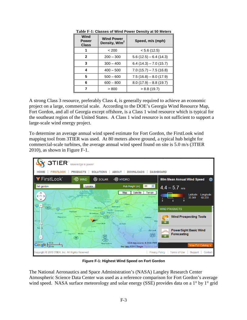
F-3

Table F-1: Classes of Wind Power Density at 50 Meters Wind

Power Class

Wind Power Density, W/m2 Speed, m/s (mph)

1 < 200 < 5.6 (12.5)

2 200 – 300 5.6 (12.5) – 6.4 (14.3)

3 300 – 400 6.4 (14.3) – 7.0 (15.7)

4 400 – 500 7.0 (15.7) – 7.5 (16.8)

5 500 – 600 7.5 (16.8) – 8.0 (17.9) 6 600 – 800 8.0 (17.9) – 8.8 (19.7)

7 > 800 > 8.8 (19.7)

A strong Class 3 resource, preferably Class 4, is generally required to achieve an economic project on a large, commercial scale. According to the DOE’s Georgia Wind Resource Map, Fort Gordon, and all of Georgia except offshore, is a Class 1 wind resource which is typical for the southeast region of the United States. A Class 1 wind resource is not sufficient to support a large-scale wind energy project.

To determine an average annual wind speed estimate for Fort Gordon, the FirstLook wind mapping tool from 3TIER was used. At 80 meters above ground, a typical hub height for commercial-scale turbines, the average annual wind speed found on site is 5.0 m/s (3TIER 2010), as shown in Figure F-1.

Figure F-1: Highest Wind Speed on Fort Gordon

The National Aeronautics and Space Administration’s (NASA) Langley Research Center Atmospheric Science Data Center was used as a reference comparison for Fort Gordon’s average wind speed. NASA surface meteorology and solar energy (SSE) provides data on a 1° by 1° grid

F-4

system, based on wind speed data over a 10-year period from July 1983 to June 1993. According to this source, the annual average wind speed in the Fort Gordon area is 3.8 m/s at 50 meters with a +/- 11% variation (NASA 2009).

Table F-2 summarizes Fort Gordon’s wind resource.

Table F-2: Summary of Wind Resource Data

Location Source Wind Speed

Fort Gordon, Georgia

State Wind Resource Map Class 1 (0.0 – 5.7 m/s at 50 m)

FirstLook tool from 3TIER 4.4 – 5.7 m/s at 80 m, 4.0 – 5.2 m/s at 50 m

NASA SSE data 3.8 m/s at 50 m

Siting Considerations The primary siting consideration for wind projects is transmission availability and the capacity of those lines. Projects need to be located within approximately 1 mile of existing transmission lines, or new lines will need to be constructed at considerable cost.

This analysis does not include any transmission costs and assumes that existing transmission lines are available to transmit power without substantial additional investment. It is also assumed that an on-site wind project would not trigger new standby or other fees from the local utility. But because wind is intermittent, the utility may have interconnection requirements to ensure grid stability and to ensure there is reliable power for the installation.

Another consideration is potential interference with airport operations. The Federal Aviation Administration (FAA) requires notice of proposed construction for a project that meets certain criteria so that it can determine if there would be adverse impacts to air navigation safety. One of the triggering criteria is whether the project would be located within 20,000 feet (3.8 miles) or less of an existing public or military airport. When selecting an area for a wind project, it would be best to avoid this potential interference issue by locating the project outside of the 20,000-foot range. Any wind project developed on-site would need to carefully consider this concern. An additional FAA criterion that would necessitate a Notice of Proposed Construction is any construction or alteration of more than 200 feet (61 meters) in height above ground level. This criterion applies regardless of the distance from the proposed project to an airport.

In response to the filing of a Notice of Proposed Construction, the FAA can either require modifications be made to the project or a “No Hazard to Air Navigation” determination can be issued and the wind project can proceed.

Wind: Economic and Other Analysis Parameters This assessment considered the current federal wind incentives: a 2.1¢/kWh renewable energy production tax credit (PTC) and 5-year accelerated depreciation. State-specific incentives for Georgia are discussed in Appendix A. During the original DoD renewable energy assessment in 2005, the installed cost of capital was approximately $1,400/kW; at the current time, prices range from $1,700 to $2,600/kW because

F-5

of high demand and increased costs for components. The capital cost was assumed to be $2,321/kW (including incentives) for this economic assessment. Because a wind energy project would provide intermittent power to the installation, the economics of a wind project are evaluated against the installation’s direct energy charge to exclude demand and other fixed charges.

Further details on the analysis methodology and the economic and incentive parameters are documented in Appendix A, and the assumptions used are listed in Table F-3.

Table F-3: Performance, Cost, and Economic Characteristics

Location Fort Gordon, Georgia

Conditions Standard: 1.225 kg/m3 density, 0°F, 0 ft elevation

Assumed Average Wind Speed 5.0 m/s at 80 m Net Capacity Factor 13.7% Turbine Type 1.5 MW, 77 m rotor, 80 m hub Project Size 1 turbine, 1.5 MW total Estimated Net Annual Energy Production 1,795,676 kWh / yr

Energy Charge 4.76¢/kWh Total Capital Cost $2,321 / kW Fixed O&M Cost $60 / kW 5-year accelerated depreciation Included Federal 2.1¢/kWh PTC Included RECs Not Included Transmission Costs Not Included

Findings: Wind The various energy cost scenarios were evaluated for ECIP eligibility and IPP project potential. To qualify for ECIP funding, a project must achieve a savings-to-investment ratio (SIR) of 1.0, and its payback is also examined. For the IPP evaluation, the commercial cost of energy was calculated to obtain an internal rate of return (IRR) of 10%. This was used as the minimum IRR required to attract the interest of a wind power project developer. Table F-4 lists the results of these analyses.

Table F-4: Economic Assessment of Wind Power

Financing Scenario

Energy Cost

(¢/kWh) IRR ECIP SIR

Simple Payback (years)

ECIP 4.76 n/a 0 623

IPP 27.75 10% n/a n/a

F-6

Wind: Next Steps As a result of the poor wind resource and unfavorable economics, Fort Gordon should not pursue a large-scale wind power project. Fort Gordon’s energy rates would have to drastically increase to make a wind project economically attractive given the area’s poor wind resource. The economic analysis of this report used the energy charge of 4.76¢/kWh. In order to reach a 10% IRR with the 5.0 m/s wind speed, even with the available incentives in Georgia, the energy rate would have to increase to 27.75¢/kWh. This is a huge rate increase and unlikely to happen.

Wind Sources of Information

3TIER. 2010. FirstLook. Accessed February 2010 at http://www.3tier.com/firstlook/.

American Wind Energy Association. 2007. “Wind Power Today.” Washington, D.C. http://www.awea.org/pubs/factsheets/WindPowerToday_2007.pdf.

American Wind Energy Association. 2008. “Wind Power Outlook.” Washington, D.C. http://www.awea.org/pubs/documents/Outlook_2008.pdf.

NREL - National Renewable Energy Laboratory. 2009. Georgia Wind Resource Map. Accessed January 2010 at http://www.windpoweringamerica.gov/images/windmaps/ga_50m_800.jpg (last updated April 10, 2009).

Federal Aviation Administration. 2007. Advisory Circular (AC 70/7460-1K) Obstruction Marking and Lighting. Effective: February 2, 2007. http://www.airweb.faa.gov/Regulatory_and_Guidance_Library/rgAdvisoryCircular.nsf/0/b993dcdfc37fcdc486257251005c4e21/$FILE/AC70_7460_1K.pdf.

Conover K, KJ Smith, TM Jurotich. November 15, 2004. U.S. Department of Defense Renewable Energy Assessment Report of Wind Energy Potential On and Near Military Installations. Global Energy Concepts, Kirkland, Washington. Subcontract No: LAM-3-32257-01.

NASA Langley Research Center. 2009. Surface meteorology and Solar Energy. Atmospheric Science Data Center. Accessed January 2010 at http://eosweb.larc.nasa.gov/sse/ (last updated August 28, 2009).

Pacific Northwest Laboratory. 1986. Wind Energy Resource Atlas of the United States. Solar Technical Information Program & Solar Energy Research Institute. Golden, Colorado. http://rredc.nrel.gov/wind/pubs/atlas/atlas_index.html.