PHYSICAL REVIEW E 85, 021908 (2012)

Nonlinear-dynamics theory of up-down transitions in neocortical neural networks

Maryam Ghorbani,1 Mayank Mehta,1,2,3,4 Robijn Bruinsma,1 and Alex J. Levine1,5

1Department of Physics and Astronomy, University of California, Los Angeles, Los Angeles, California 90095-1547, USA2Department of Neurology, Department of Neurobiology, University of California, Los Angeles, Los Angeles, California 90095-1547, USA

3Integrative Center for Learning and Memory, University of California, Los Angeles, Los Angeles, California 90095-1547, USA4Keck Center for Neurophysics, University of California, Los Angeles, Los Angeles, California 90095-1547, USA

5Department of Chemistry and Biochemistry, University of California, Los Angeles, Los Angeles, California 90095-1547, USA(Received 7 July 2011; revised manuscript received 30 November 2011; published 13 February 2012)

The neurons of the neocortex show ∼1-Hz synchronized transitions between an active up state and a quiescentdown state. The up-down state transitions are highly coherent over large sections of the cortex, yet they areaccompanied by pronounced, incoherent noise. We propose a simple model for the up-down state oscillationsthat allows analysis by straightforward dynamical systems theory. An essential feature is a nonuniform networkgeometry composed of groups of excitatory and inhibitory neurons with strong coupling inside a group and weakcoupling between groups. The enhanced deterministic noise of the up state appears as the natural result of theproximity of a partial synchronization transition. The synchronization transition takes place as a function of thelong-range synaptic strength linking different groups of neurons.

DOI: 10.1103/PhysRevE.85.021908 PACS number(s): 87.19.L−, 05.45.−a, 87.18.Sn

I. INTRODUCTION

The theory of dynamical systems has been widely appliedto analyze the activity of neurons. A variety of simple modelequations that describe the electrical potential and ioniccurrents associated with the firing of a neuronal action potentialspike exhibit a form of bifurcation [1]. Most bifurcation typespossible for two-component dynamical systems have beenobserved for different types of neurons in different sections ofthe brain [2]. The model equations are enormously simplifiedbut the bifurcation classification incorporates general math-ematical principles that have more general validity than theequations themselves. The application of dynamical systemstheory to networks of coupled neurons is currently a very activearea of research, in particular, in the context of synchronizationbetween networks. Simple neural circuits, such as the onethat regulates the breathing rhythm, can be readily analyzed,again by applying the methods of dynamical systems theory tosimplified equations [2]. However, analyzing the functionallycomplex neural circuitry of the cortex is obviously much morechallenging. A full theory of cortical neural dynamics should,for example, address far-reaching questions such as the natureof computation executed by spike-timing.

In this paper, we focus instead on the application ofdynamical systems theory to collective neural activity insidethe cortex section of the brain. An important and common wayto characterize the collective activity of the cortex is presentedby the electroencephalograph (EEG). An EEG records voltagefluctuations [3] measured on the surface of the skull. Similarsignals, called local field potentials (LFPs), are measured bymicrowires inserted into the cortex. EEG and LFP recordingsreflect the average activity of a large ensemble (>104) ofneurons surrounding the measurement sites. The signalstypically span a frequency range between 0.1 and 300 Hz witha spectral power that increases with decreasing frequency [4].

A striking feature of cortical EEGs and LFPs recordedduring slow-wave sleep and anesthesia is regular, large-scaleoscillations with a low-frequency range (0.5–2 Hz) and largeamplitude (∼1 mV in EEG). They are known as delta

oscillations or slow-wave-sleep (SWS) oscillations [5]. Theoscillations are coherent across large parts of the cortex andcan also be seen in measurements of the membrane potentialsof individual neurons [5–7]. Figure 1 shows an example of anintracellular recording of the membrane potential of a singleneuron (from Ref. [8]) taken during a period of slow EEGoscillations.

The recording shows that the membrane potential of an indi-vidual neuron undergoes repetitive transitions from a quiescent“down” state to a noisy “up” state with a number of spikes. Theresting potential of a neuron with respect to the surroundingextracellular fluid is around −70 mV. During a down state, aneuron has a membrane potential a few mV below this restingpotential and is said to be hyperpolarized. Next, if the cell is de-polarized beyond a threshold of around −55 mV, it will start tofire action potentials (∼100-mV amplitude, ∼1-ms duration)that will travel down the axon. Figure 1 shows that during anup state, a cell occasionally fires an action potential. As shownin Fig. 2, the action potentials, also known as spikes, travelfrom the cell body (“soma”) down the axon to another neuron.

The terminals of the axon are connected by synapticjunctions to the dendrites of the other neuron (see the insetof Fig. 2). If the initial neuron was excitatory, then the signalhas a depolarizing effect, known as an excitatory postsynapticpotential (EPSP). If the initial neuron was inhibitory, thenthe signal typically has a hyperpolarizing effect, known as aninhibitory postsynaptic potential (IPSP). The total dendriticinput determines whether or not the membrane potential ofthe second neuron will be sufficiently depolarized for it toreach spiking threshold [5]. In a well-connected networkof excitatory neurons, positive feedback between differentexcitatory neurons would produce a burst of action potentialfirings with a frequency in the 10–100 Hz range. In the up statethis does not happen: The (mean) membrane potential remainsa few mV below the firing threshold and, on average, a neuronwill fire at most one action potential during an up state [8].Control of the level of positive feedback is clearly a necessaryfeature of up states.

021908-11539-3755/2012/85(2)/021908(14) ©2012 American Physical Society

GHORBANI, MEHTA, BRUINSMA, AND LEVINE PHYSICAL REVIEW E 85, 021908 (2012)

FIG. 1. Whole cell (WC) recording from Ref. [8] of the mem-brane potential of layer 2/3 pyramidal neurons of a rat. The up-downstate oscillations have an average period of about 1 s. The “up” stateshave a mean amplitude of about +20 mV relative to the membranepotential in the “down” state and they show noisy fluctuations due toa rapid barrage of postsynaptic potentials. In the less noisy “down”states, the neurons are hyperpolarized with a mean potential of−71 mV. The number of action potentials fired by a neuron perup state is typically small, on the order of one. For example, in thelower trace (WC2), we see a single action potential (narrow spike)produced during the second and fourth of the five up states shown.

The repeated cycling between the up-state and down-statepotentials is known as up-down state (UDS) oscillations[4]. Under the influence of several anesthetics and duringthe slow-wave sleep, large-amplitude, 0.5–2 Hz oscillationsare present in the EEG in many species including humans,primates, and rodents. These oscillations can also be seenin the neocortical LFP reflecting synchronous changes inthe membrane potentials of large neuronal ensembles. Dur-ing these slow oscillations the neural activity, such as themembrane potential and spiking probability, exhibit bistabilitysuch that large ensembles of neurons synchronously maketransitions between a more depolarized and more active upstate, and a less depolarized and less active down state[5,10]. All types of neurons in the neocortex, including theexcitatory and inhibitory neurons’ membrane potentials, showvirtually synchronous transitions. In other words, excitatoryand inhibitory neurons become more active in the up state andless active in the down state [11–13].

Due to their reliable synchrony across many brain areasand neural types, the up-down state transitions have been usedto probe the functional connectivity and dynamics of corticalcircuits. They could explain some amount of variability ofneural responses to stimuli [8,14–16]. Further, it is believedthat during the UDS the neocortex and hippocampus interactto facilitate the long-term consolidation of recently formedmemories [17–26]. Early studies described the UDS in termsof the membrane potential of excitatory neurons. Later studiesshowed that during UDS, the spiking probabilities of bothexcitatory and inhibitory neurons changes synchronously.Hence, UDS can also be detected using the firing rates of largeensembles of neurons [27–30], which results in concomitanttwo-state oscillations in the LFP [19,21,31,32].

FIG. 2. (Color online) Drawing of a pair of neurons. When themembrane potential of the body (“soma”) of the neuron at the topexceeds the firing threshold, an action potential is generated thattravels along the axon of the first neuron to the dendrites of thesecond neuron. Inset: A synaptic junction between an axonal terminalof one cell and the dendrite of a second neuron. When the electricalsignal reaches the terminal, neurotransmitters are released into thesynaptic cleft and they bind with neuroreceptors in the postsynapticneuron. This generates an excitatory postsynaptic potential (EPSP)that is depolarizing if the signal comes from an excitatory neuronand an inhibitory postsynaptic potential (IPSP) that is typicallyhyperpolarizing if it comes from an inhibitory neuron. (Image fromRef. [9].)

Observations on UDS oscillations can be summarized asfollows.

(i) In the active (up) state of the cycle, individual neo-cortical neurons fire rarely, with a typical rate that is lessthan 1 Hz [8]. The cell body receives from its dendrites anavalanche of EPSPs and IPSPs, which explains the noise inthe up state in Fig. 1. The mean membrane potential of theneuron remains somewhat below threshold in the up state, asalready mentioned [8]. One of the questions we will addressis how membrane potentials can be regulated in a robust wayto lie just below the firing threshold.

(ii) In the less active (down) state, the membrane potentialof all neuron types is in a prolonged hyperpolarized state withlittle evidence of EPSPs and IPSPs [5,8]. Neurons rarely firea spike during the down state. Thus the membrane potential isessentially biphasic, shuttling between two values during theup-down states.

(iii) The up-state activity is regulated by the inhibitoryneurons. Pharmacological reduction in the level of inhibition

021908-2

NONLINEAR-DYNAMICS THEORY OF UP-DOWN . . . PHYSICAL REVIEW E 85, 021908 (2012)

results in increased spiking [8]. Complete suppression ofinhibition results in an up state state with no up-down stateand almost continuous spiking.

(iv) The UDS oscillations are synchronous over largeportions of the cortex [8]. The duration of the up state andthe oscillation period show significant variability from cycleto cycle.

The precise mechanism(s) that terminates an up stateafter about 1 s has not been completely determined. Thecandidate mechanism we focus on here is dendritic spikefrequency adaptation (DSFA) [33,37]: Incoming action po-tentials produce an increase in the outward conductance of thedendritic membrane. Experiments report that spike frequencyadaptation is shown by virtually all the cortical excitatoryneurons, but rarely by the inhibitory neurons. This increasedconductance, which may be due to activation of K+ channelsor to a local increase of Ca2+, reduces the ability of thedendritic synaptic junctions of excitatory neurons to generatepostsynaptic potentials. DSFA may also be due to the depletionof neurotransmitters in the synaptic clefts.

The UDS oscillations pose a puzzle for a dynamical systemsdescription: They combine collective, highly synchronizedregularity with pronounced noise in individual neurons. Thisswitching between up and down states appears not to beexternally regulated, which would have been the simplestexplanation. Qualitatively similar slow oscillations—althoughof lower frequency—are also seen in vitro in isolated, small(<mm2) slices of the neocortex [6]. For the same reason, theup-state noise is also of an intrinsic nature: Individual neuronsare essentially deterministic so the noise, as the up-down stateswitching, must be a collective property of an ensemble ofneurons. Simple models of coupled oscillatory networks reportthat when the coupling strength is increased, one encounterssynchronization through phase locking, as exhibited, forexample, by the Kuramoto Model [2,38]. It is difficult tosee, however, how one can reconcile the deterministic noisepresent during the up states with the regularity of the collectiveswitching between the up and down states.

In this paper we present a simple theoretical framework forup-down state dynamics of cortical neural circuits consistentwith the features (i)–(iv) listed above. The model is basedon DSFA but does not rely on any detailed properties ofDFSA [37]. We only assume that (i) synaptic activity in theup state progressively reduces the ability of excitatory (but notinhibitory) neurons to respond to depolarizing synaptic inputs,resulting in the termination of the up state, and (ii) that duringthe down state, a separate process, such as the activity of Ca2+pumps, slowly restores the ability of a neuron to respond tosynaptic input. This results in a gradually increased excitabilityof the network and an eventual transition to the up state.

There are several possible sources of such adaptation:synaptic, somatic, and dendritic. In vitro studies show thatall three mechanisms are present in the excitatory neurons.There is little evidence that these three occur in a majorityof neocortical inhibitory neurons. This unequal short-termdynamics is the key ingredient responsible for the terminationof up states in our model. We believe that all three ofthem can contribute to this process. Further, given the verylow firing rates of excitatory neurons (∼1 Hz), excitatoryneurons will fire about one spike per up state, which would

not result in a substantial amount of synaptic and somaticadaptation. However, thousands of excitatory inputs terminateon the dendrites. The dendrites of excitatory neurons havevoltage-gated channels, many of which are similar to thosein the soma, such as the voltage-gated potassium channels,that are responsible for spike frequency adaptation. Hence,we hypothesize that the summation of a large number ofexcitatory inputs on excitatory neurons’ dendrites results inthe depolarization of dendrites in the up state, which islikely to engage the dendritic spike frequency adaptationmechanism. The inhibitory synapses mostly terminate on thesoma so the dendritic mechanisms would not influence muchthe inhibitory-inhibitory (I-I) and inhibitory-excitatory (E-I)synapses. Hence we hypothesize that the dendrites wouldbe far more active than either the synapses or the somain the adaptation of the excitability of the excitatory butnot the inhibitory neurons. Further, most inhibitory neurons’soma do not show spike frequency adaptation so excitatory-inhibitory (I-E) synapses would not show adaptation either.Thus the dendritic spike frequency adaptation mechanism islikely to influence the excitatory-excitatory (E-E) synapses.In this simple averaged neuron model, we have modeled thisphenomenon by the adaptation of E-E synapses, which resultsin an effective decay of excitatory synapses with increasingduration in the up state. This does not rule out the contributionof other mechanisms to adaptation.

The central result of our paper is that for nonuniformnetworks composed of groups of excitatory and inhibitoryneurons with strong coupling inside each group but weakcoupling between groups, we encounter a partial synchro-nization transition associated with the onset of coherent UDSoscillations at very weak “long-range” synaptic coupling.Strong deterministic noise appears near the synchronizationthreshold due to dephased oscillatory activity of the individualnetworks. As the coupling strength increases, synchronizationof all up-state activity does take place via a Kuramoto-typetransition, but this requires making the long-range synapticstrength equal to the short-range synaptic strength. Up-statedeterministic noise disappears in this limit.

The paper is organized as follows. In Sec. II we present themodel. In Sec. III, we discuss the dynamics and phase diagramfor the case of a uniform network of neurons. In Sec. IVwe examine the properties of coupled groups of neurons andpresent the evidence for a synchronization transition combinedwith the appearance of deterministic noise in the up states.

II. POINT-NEURON MODEL WITH ADAPTATION

In this section we present the equations for a network ofneurons in the presence of DSFA. Excitatory neurons will berepresented by two dynamical variables: a “fast” membranepotential v(t) of the soma of the neuron and a “slow” adaptationparameter c(t) that measures the degree of adaptation of thedendrites of the excitatory neurons to prolonged input. Incontrast, inhibitory neurons are represented only by a fastmembrane potential with no adaptation variable. The DSFAprocess is described as follows. In the down-state part of thecycle, the adaptation level c(t) is sufficiently high for excitatoryneurons to be unable to stimulate other excitatory neurons.Neural activity dies down and only very weak, residual, firing

021908-3

GHORBANI, MEHTA, BRUINSMA, AND LEVINE PHYSICAL REVIEW E 85, 021908 (2012)

activity remains. The time scale for the down part of thecycle is determined by the recovery time of the adaptationprocess, which is taken to be in the range of seconds (e.g., thetime scale required for pumping out excess Ca2+). When c(t)has been sufficiently reduced, excitatory neurons can start toactivate each other, initiated by a low residual firing activity.Excitatory postsynaptic potentials (EPSPs) are generated as aresult. Inhibitory neurons become active as well and start togenerate inhibitory postsynaptic potentials (IPSPs), with themembrane potential v(t) of both types of neurons remainingbelow threshold. The adaptation parameter now starts to risedue to EPSPs generated by excitatory neurons. This graduallysuppresses the up-state positive feedback between excitatoryneurons causing the up state to die down, after which the cyclestarts again.

A. Model equations

We will separately discuss the rate equations obeyed by v(t)and c(t). The membrane potential vn

e (t) of the nth excitatoryneuron of the network is assumed to obey—apart from theDSFA process—the conventional rate equation of the pointneuron model:dvn

e

dt= − 1

τe

vne +

∑m

J nmee (cn)rm

(vm

e

) +∑

k

J nkei rk

(vk

i

). (2.1)

Inhibitory neurons obey a similar equation:

dvni

dt= − 1

τi

vni +

∑k

J nkii rk

(vk

i

) +∑m

J nmie rm

(vm

e

). (2.2)

Note that there is no dependence on the adaptation variable inEq. (2.2). The spiking rate tracks the time-averaged subthresh-old membrane potential, as evidenced by a vast amount ofliterature. Thus vk

e,i is the time-averaged subthreshold potentialof the kth excitatory (e) or inhibitory (i) neuron.

In these two equations, the first term on the right-hand side(RHS) represents the relaxation of the membrane potentialto its equilibrium value. The membrane relaxation timeconstants τe and τi (with τe ∼ 20 ms for excitatory neuronsand τi ∼ 10 ms for inhibitory neurons) are much shorter thanthe time scale of the up-down state oscillations. The restingpotential will be assumed to be the same for all neurontypes and all potentials will be measured with respect to thecommon resting potential. Positive and negative values for v

thus correspond to depolarized and hyperpolarized membranepotentials, respectively. The second and third terms on theRHS represents the rate of change of the membrane potentialdue to EPSPs and IPSPs. The sums are over all neuronsm that make a synaptic connection to neuron n. Here, rn

is the voltage-dependent firing rate of neuron n. Next, thestrengths of synaptic connections from neuron m to neuronn are given by the matrix elements J nm (superscripts willalways refer to the neuron index). Positive (negative) entriescorrespond to excitatory (inhibitory) input. The subscripts ee,ii, ie, and ei of the matrix elements denote, respectively,synaptic connections from excitatory to excitatory neurons(Jee, positive), from inhibitory to inhibitory neurons (Jii ,negative), from excitatory to inhibitory (Jie, positive), andfrom inhibitory to excitatory junctions (Jei , negative). Onlythe excitatory-excitatory synapses are assumed to be subject

to DSFA so only Jee(c) depends on the adaptation parameter.For these excitatory-excitatory matrix entries, the synapticstrength will be assumed to rapidly decrease if the adaptationparameter c exceeds a threshold c∗. We will assume asigmoidal dependence on c:

Jee(c) = Jee(0)

1 + exp[(c − c∗)/gc]. (2.3)

The parameter gc, the width of the transition region, can bevaried to examine the dependence of up-down state dynamicson the sharpness of the onset of adaptation. In the numericalresults discussed below, we took gc equal to 3 and verified thatour results were not qualitatively altered when we allowed gc tovary. The parameter c∗ is the value of the adaptation parameterwhere the synaptic strength has dropped by a factor of 2 fromits maximum value Jee(0) (we used c∗ = 10). Recall from ourearlier discussion that one should expect c to oscillate aroundc∗. We will use the maximum synaptic strength Jee(0) as thecentral control parameter. It measures the maximum possiblepositive feedback between excitatory neurons. The particularfunctional form of Eq. (2.3) would follow from a two-state“open-closed” model [39] for adaptation but the precise formis not essential. Next, the dependence of the firing rate of aneuron on its membrane potential will be assumed to be of astandard form

r(ve,i) = rm

1 + exp[−(ve,i − v∗)/ge,i]. (2.4)

Here, rm (∼70 Hz) is the maximal firing rate in a completelydepolarized state while v∗ is the threshold firing potential.We find that ge > gi (i.e., the firing rate dependence on themembrane potential is sharper for the inhibitory neurons thanit is for the excitatory ones) is required to ensure the stabilityof the UDS oscillations within the model. This remains to betested and constitutes a prediction necessary for the validity ofour approach. The assumption is consistent with the commonobservation that inhibitory neurons typically have higher firingrates than excitatory neurons in vivo. For the numerical workpresented here, we fix ge = 5 mV for excitatory neurons andgi = 2 mV for inhibitory neurons.

For the rate equation of the adaptation parameter forexcitatory-excitatory synapses, we use a description similarto that of Fuhrmann et al. [36]:

dcn

dt= − 1

τc

cn + �c∑m

rme

(vm

e

). (2.5)

Here, cm represents the mean adaptation level of the excitatory-excitatory synapses of excitatory neuron m. The adaptationrecovery time τ c will be taken to be 0.5 s. The sum on the RHSis over the excitatory neurons that make a synaptic junctionwith neuron n. The increase of the mean adaptation parameter�c per incoming action potential will be a second importantcontrol parameter.

III. UNIFORM NETWORKS OF EXCITATORY ANDINHIBITORY NEURONS

In this section we will examine the equations presented inSec. II, first analytically and then numerically, for the case oftwo coupled, uniform networks. The first network is composed

021908-4

NONLINEAR-DYNAMICS THEORY OF UP-DOWN . . . PHYSICAL REVIEW E 85, 021908 (2012)

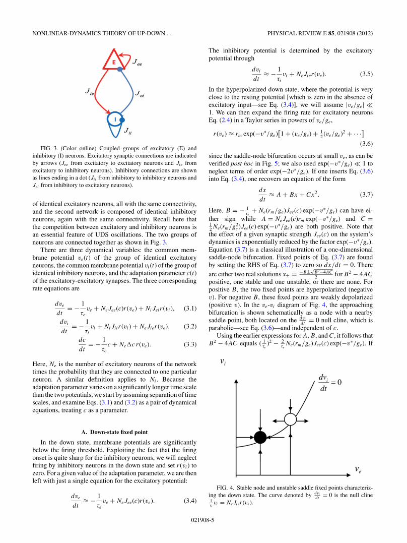
FIG. 3. (Color online) Coupled groups of excitatory (E) andinhibitory (I) neurons. Excitatory synaptic connections are indicatedby arrows (Jee from excitatory to excitatory neurons and Jie fromexcitatory to inhibitory neurons). Inhibitory connections are shownas lines ending in a dot (Jii from inhibitory to inhibitory neurons andJei from inhibitory to excitatory neurons).

of identical excitatory neurons, all with the same connectivity,and the second network is composed of identical inhibitoryneurons, again with the same connectivity. Recall here thatthe competition between excitatory and inhibitory neurons isan essential feature of UDS oscillations. The two groups ofneurons are connected together as shown in Fig. 3.

There are three dynamical variables: the common mem-brane potential ve(t) of the group of identical excitatoryneurons, the common membrane potential vi(t) of the group ofidentical inhibitory neurons, and the adaptation parameter c(t)of the excitatory-excitatory synapses. The three correspondingrate equations are

dve

dt= − 1

τe

ve + NeJee(c)r(ve) + NiJeir(vi), (3.1)

dvi

dt= − 1

τi

vi + NiJiir(vi) + NeJier(ve), (3.2)

dc

dt= − 1

τc

c + Ne�c r(ve). (3.3)

Here, Ne is the number of excitatory neurons of the networktimes the probability that they are connected to one particularneuron. A similar definition applies to Ni . Because theadaptation parameter varies on a significantly longer time scalethan the two potentials, we start by assuming separation of timescales, and examine Eqs. (3.1) and (3.2) as a pair of dynamicalequations, treating c as a parameter.

A. Down-state fixed point

In the down state, membrane potentials are significantlybelow the firing threshold. Exploiting the fact that the firingonset is quite sharp for the inhibitory neurons, we will neglectfiring by inhibitory neurons in the down state and set r(vi) tozero. For a given value of the adaptation parameter, we are thenleft with just a single equation for the excitatory potential:

dve

dt≈ − 1

τe

ve + NeJee(c)r(ve). (3.4)

The inhibitory potential is determined by the excitatorypotential through

dvi

dt≈ − 1

τi

vi + NeJier(ve). (3.5)

In the hyperpolarized down state, where the potential is veryclose to the resting potential [which is zero in the absence ofexcitatory input—see Eq. (3.4)], we will assume |ve/ge| �1. We can then expand the firing rate for excitatory neuronsEq. (2.4) in a Taylor series in powers of ve/ge,

r(ve) ≈ rm exp(−v∗/ge)[1 + (ve/ge) + 1

2 (ve/ge)2 + · · ·](3.6)

since the saddle-node bifurcation occurs at small ve, as can beverified post hoc in Fig. 5; we also used exp(−v∗/ge) � 1 toneglect terms of order exp(−2v∗/ge). If one inserts Eq. (3.6)into Eq. (3.4), one recovers an equation of the form

dx

dt≈ A + Bx + Cx2. (3.7)

Here, B = − 1τe

+ Ne(rm/ge)Jee(c) exp(−v∗/ge) can have ei-ther sign while A = NeJee(c)rm exp(−v∗/ge) and C =12Ne(rm/g2

e )Jee(c) exp(−v∗/ge) are both positive. Note thatthe effect of a given synaptic strength Jee(c) on the system’sdynamics is exponentially reduced by the factor exp(−v∗/ge).Equation (3.7) is a classical illustration of a one-dimensionalsaddle-node bifurcation. Fixed points of Eq. (3.7) are foundby setting the RHS of Eq. (3.7) to zero so dx/dt = 0. Thereare either two real solutions x± = −B±√

B2−4AC2 for B2 − 4AC

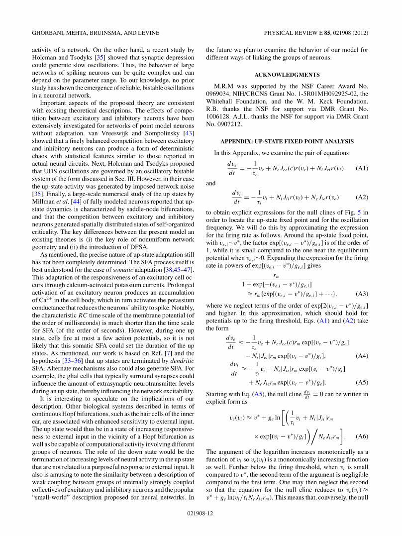
positive, one stable and one unstable, or there are none. Forpositive B, the two fixed points are hyperpolarized (negativev). For negative B, these fixed points are weakly depolarized(positive v). In the ve-vi diagram of Fig. 4, the approachingbifurcation is shown schematically as a node with a nearbysaddle point, both located on the dvi

dt= 0 null cline, which is

parabolic—see Eq. (3.6)—and independent of c.Using the earlier expressions for A, B, and C, it follows that

B2 − 4AC equals ( 1τe

)2 − 2τe

Ne(rm/ge)Jee(c) exp(−v∗/ge). If

FIG. 4. Stable node and unstable saddle fixed points characteriz-ing the down state. The curve denoted by dvi

dt= 0 is the null cline

1τi

vi = NeJier(ve).

021908-5

GHORBANI, MEHTA, BRUINSMA, AND LEVINE PHYSICAL REVIEW E 85, 021908 (2012)

FIG. 5. (Color online) (a) Null clines of the excitatory and inhibitory potentials during an up state (upper solid circle). The up state ischaracterized by a stable spiral fixed point. A down-state saddle-node pair (solid and open circle) has just appeared by a saddle-node bifurcationso the system is bistable. (b) As the adaptation parameter c continues to increase, the saddle begins to move rightward along the vi = 0null cline and will eventually annihilate the up-state fixed point. (c) Null clines at the saddle-node bifurcation that destabilized the up state.(d) Up-down states of the uniform network model. Parameters were tuned so (i) the up-state potential remains somewhat below the firingthreshold of 30 mV and (ii) the decay time of the up-state weakly overdamped oscillation is long compared to the period. The system is closeto a Hopf bifurcation where the up-state activity would turn into a limit cycle.

Jee(c) is increased, B2 − 4AC decreases and the two fixedpoints merge when the synaptic strength reaches a criticalvalue

J ∗ ∼ ge

2Neτerm

exp(v∗/ge). (3.8)

For Jee(c) larger than J ∗ there are no fixed points associatedwith the down state. Both inhibitory and excitatory potentialsthen flow to an up-state fixed point close to the firing threshold,as discussed below.

B. Up-state fixed point

Start from an initial state where there are no down-statefixed points (so B2 < 4AC). The rate equations cause thesystem to flow to the up-state fixed point. In that regime, theadaptation parameter is (slowly) increasing. This leads to aslow decrease of Jee(c) and thus of B. Eventually B falls below−2

√AC and the down-state saddle-node pair reappears. This

does not terminate the up state, however. The mathematicalanalysis of the up-state fixed point is more involved than thatof the down-state fixed point and is give in the Appendix. Here,we will illustrate the results combining numerical solution withsimple arguments.

Figure 5(a) shows the numerically obtained null clinesdvi

dt= 0 and dve

dt= 0 for a value of c in the ve-vi diagram where

the down-state saddle-node pair has just reappeared (analyticexpressions for the null clines are given in the Appendix).

In Figs. 5(a) and 5(b), the up-state fixed point is shown asthe top intersection of the two null clines, somewhat below thefiring threshold at 30 mV. A pair of down-state fixed pointshas just appeared at the lower left-hand corner in Fig. 5(a).The evolution of those fixed points with increasing c is shownin Fig. 5(b). In the Appendix the membrane potentials of theup-state fixed point are shown to be

v∗i − v∗ ≈ −gi ln[τirmNiJie|Jei |/Jee(c)gi], (3.9a)

v∗e − v∗ ≈ −ge ln(τirmNeJie/gi). (3.9b)

Note that Eq. (3.9a) but not (3.9b) depends on the adaptationparameter. Equation (3.10) shows for what combination ofsynaptic strengths the operating point of the network areset somewhat below the firing threshold v∗: The dimen-sionless parameters �i ≡ [τirmNiJie|Jei |/Jee(c)gi] and �e ≡(τirmNeJie/gi) both have to exceed one. In that case thefixed-point potentials are located roughly within a distancegi,e of the firing threshold.

This last result is important. Because the logarithmicfunction is only weakly dependent on its argument, locating

021908-6

NONLINEAR-DYNAMICS THEORY OF UP-DOWN . . . PHYSICAL REVIEW E 85, 021908 (2012)

the fixed point somewhat below the firing threshold is quite“robust:” The fixed point hardly shifts if the synaptic strengthsare changed as long as the two parameters exceed one.Individual neurons do not have a “natural” setting for themembrane potential to be pegged a bit below the firingthreshold. The stability of this setting is produced here bythe interplay between the excitatory and inhibitory neurons.Note that by allowing these parameters to drop below one, italso is possible to significantly “turn up” the firing rate, asmight happen during awakening.

In a linear stability analysis of this fixed point (v∗e ,v

∗i ), small

deviations around the new fixed point are described by(δve

δvi

)=

(a11 a12

a21 a22

)(δve

δvi

). (3.10)

Here, a11 = − 1τe

+ NeJee(c)r ′(v∗e ), a12 = NiJeir

′(v∗i ), a21 =

NeJier′(v∗

e ), and a22 = − 1τi

+ NiJiir′(v∗

i ). The eigenvalues

λ1,2 = Tr±√

Tr2−4�

2 , with Tr = a11 + a22 the trace and � =a11a22 − a12a21 the determinant, determine the fate of smalldeviations of the fixed point. The slope of the dvi

dt= 0 null

cline must exceed the slope of the dve

dt= 0 null cline at

the fixed point in order for there to be an intersection [seeFig. 5(a)]. The equation for the dvi

dt= 0 null cline is, according

to Eq. (3.10), a11δve + a12δvi = 0, and that of the dve

dt= 0

null cline a21δve + a22δvi = 0. The dvi

dt= 0 null cline has the

largest slope if (− a11a12

) is less than (− a21a22

). According to this lastcondition, the sign of the determinant � = a11a22 − a12a21 hasto be positive, keeping in mind that both a11/a12 and a21/a22

are negative. This means that the eigenvalues either are bothreal with the same sign—in which case the fixed point is againa node—or that they are complex conjugates, in which casethe trajectories must spiral either in or out. Drawing the flowvectors in Fig. 5(b) produces spiral trajectories correspondingto overdamped oscillations. The eigenvalues are complexconjugates, which means that Tr2 − 4� must be negative.

The imaginary part � = 12

√4� − Tr2 of the eigenvalue is the

frequency scale of the oscillations in the up state. For negativevalues of the trace, the real part of the eigenvalues is negative

and the up-state fixed point corresponds to a stable spiral. Theflow lines spiral inward to the fixed point with a characteristictime scale equal to −2/Tr. For positive values of the trace,the flow lines spiral outward and approach a limit cycle: Thepoint Tr = 0 marks a Hopf bifurcation. The “critical regime,”with Tr small compared to the oscillation frequency �, is theappropriate operating point for the start of the up-state period,in a theory of up-state activity with persistent oscillatoryactivity due to competition between inhibitory and excitatoryneurons.

In the Appendix, the matrix elements are shown to be givenapproximately by

a11 ≈ − 1

τe

+ 1

τi

(gi

ge

)Jee(c)

Jie

, (3.11)

a12 ≈ − 1

τi

Jee(c)

Jie

, (3.12)

a22 ≈ − 1

τi

− 1

τi

|Jii |Jee(c)

Jie|Jei | , (3.13)

a21 ≈ 1

τi

. (3.14)

The decay rate of the oscillation is given by

−Tr ≈ 1

τe

+ 1

τi

− 1

τi

Jee(c)

Jie

[(gi

ge

)− |Jii |

|Jei |]

. (3.15)

Setting the trace to zero is possible only if the inhibitory-inhibitory synaptic coupling is sufficiently weak compared tothe coupling between inhibitory and excitatory neurons, i.e.,if |Jii |

|Jei | < ( gi

ge). Assuming that this is the case, the condition of

vanishing trace is

Jee(c)

Jie

≈(

τi

τe

+ 1

)/[(gi

ge

)− |Jii |

|Jei |]

. (3.16)

If this condition is not quite obeyed, then the decay rateof the oscillation is equal to the trace. Note that increasingthe adaptation parameter increases the decay rate of theoscillation, an effect visible in Fig. 5(c). Assuming that thetrace has been set to zero, the resulting oscillation frequency� ≈ √

(a11a22 − a12a21) is

� ≈ 1

τi

√[τi

τe

−(

gi

ge

)Jee(c)

Jie

] (1 + |Jii |Jee(c)

Jie|Jei |)

+(

Jee(c)

Jie

) (gi

ge

). (3.17)

A particular simple case occurs when one can neglectinhibitory-inhibitory coupling (i.e., Jii = 0). In that case wefind that the oscillation frequency

� ≈ 1√τeτi

(3.18)

is set by the geometrical mean of the excitatory and inhibitorymembrane relaxation times, which is in the range of 10–100 Hz. The full solution with corrections due to the small,but nonzero, Jii is shown in the Appendix. Examining thatsolution, we note that the oscillation frequency is generically

larger than the geometric mean [Eq. (3.18)], but decreasestoward that value near the termination of the up state.

We now consider the termination of the up state in moredetail. An increase in the adaptation parameter c causes Jee(c)to decrease and the oscillation frequency to decrease. This isshown most simply by noting that the magnitude of the traceincreases and must be included in the oscillation frequency

since � = 12

√4� − Tr2. The spiral fixed point turns into a

stable node when Tr2 = 4�, at which point the eigenvalues ofthe matrix become real and oscillations stop. At the same time,the unstable fixed point moves up along the null cline dvi

dt= 0,

021908-7

GHORBANI, MEHTA, BRUINSMA, AND LEVINE PHYSICAL REVIEW E 85, 021908 (2012)

as discussed above in Fig. 4. As discussed in the Appendix,the unstable fixed point is marked by a logarithmic singularityof the null cline.

The unstable fixed point fuses with the up-state fixed pointwhen the two null clines share a common tangent, which isthe case when � = 0. This marks a new bifurcation where theup-state fixed point disappears. Figure 5(c) shows an examplewhere the stable and unstable fixed points have just fusedthrough a saddle-node bifurcation. In the Appendix we showthat this bifurcation is determined by the condition that Jee(c)drops below a threshold J ∗

ee ≡ (geτi/giτe)Jie. For values ofJee(c) below J ∗

ee, the flow lines drive the system back to thestable down-state fixed point, after which the cycle starts again.

A picture emerges of a sequence of up-down state oscilla-tions as a periodic cycle where an unstable fixed point shuttlesup and down the dvi

dt= 0 null cline, alternatingly destroying

the down-state and the up-state stable fixed points through aseries of repeated saddle-node bifurcations. In order to verifythis analysis, we carried out a numerical analysis of the fullset of equations. Figure 5(c) shows two successive periods,computed numerically. The coexistence of the two stable fixedpoints separated by an unstable fixed point, shown by the firstarrow, corresponds to Fig. 5(a). The unstable fixed point slidesup the null cline and, at the point indicated by the second arrow,at the end of the up cycle, it annihilates the stable fixed pointof the up state, corresponding to Fig. 5(b), consistent with ouranalysis. For the choice of parameters for Fig. 5(c), the up-stateoscillations clearly are weakly underdamped with |Tr| � �:The system is close to a Hopf bifurcation. The excitatory andinhibitory oscillations track each other while the adaptationparameter slowly oscillates around the set point c∗=10.

The sequence of up-down states of Fig. 5(c) appears tobe strictly periodic, but this is not the case. If one tracksthe trajectory over many successive cycles in the vi-ve

plane, computed numerically, then an irregular precession ofoscillatory orbits is encountered, shown in Fig. 6(a).

This irregular precession is in fact visible in a plot of thefiring rate, as shown in Fig. 6(b). The fact that the orbits

FIG. 6. (Color online) (a) Trajectory of the excitatory andinhibitory potentials for the same parameters as Fig. 5 but now formany periods. The up-state activity shows as a spiral trajectory endingat the up-state fixed point at the upper right-hand corner. The failure ofthe up-state orbits to close means that the system cannot be describedperfectly as two dimensional (see text). The down-state fixed pointis at the lower left-hand corner. (b) The precession of the potentialmaxima is visible in the firing rate, which is dominated by the maximaof the potential.

FIG. 7. (Color online) Membrane potential as a function of timeif the excitatory synaptic strength slowly increases.

in the ve-vi fail to close exactly must mean, according tothe Poincare-Bendixson theorem [1], that, notwithstanding thedifference in time scales between the adaptation parameterand the rapid up-state oscillations, the dynamics cannot bedescribed by only two coupled equations. However, Fig. 5(c)demonstrates that these effects are difficult to see in a recordingof the membrane potential.

One could speculate that this model for up-down stateoscillations could be used as a simple description for thegradual awakening from deep sleep (or anesthesia) by aslow increase of the positive feedback between excitatoryneurons, i.e., by increasing the synaptic strength Jee(0) linkingexcitatory neurons. We assume that Jee(0) slowly increasesas animals become more awake. This could be mediated by avariety of cellular mechanisms. For example, neuromodulatorschange neural excitability as well as short-term plasticity.The neuromodulator concentrations change with behavioralstate and thus can alter the strength of neural connectivity.This modulation can influence differentially the excitatoryand inhibitory neurons. For instance, acetylcholine alters theexcitatory neurons’ spike frequency adaptation and cholinergiclevels change with the sleep-wake cycle. Dopamine has adistinct effect on excitatory and inhibitory inputs. As shown inFig. 7, the model predicts that the UDS period shortens whenJee(0) increases, while the fraction of time spent in the downstate goes to zero.

There is a point where the down state completely disap-pears, leaving the system permanently in the up state, still withrapid oscillations due to the feedback between excitatory andinhibitory neurons. These are in fact features that have beenreported in studies of awakening and, in a future publication,we will compare theory and experiment.

An important problem with the uniform network descrip-tion of this section is that the computed activity of the up-statepotential is much more regular than the measured noisyup-state activity displayed in Fig. 1. In fact, there is littleresemblance between Figs. 1 and 5(c). In the next section, wewill show that network geometry plays a crucial role in termsof up-state activity.

IV. SYNCHRONIZATION TRANSITION

In this section we will examine the model for the simplestcase of a nonuniform network: two weakly coupled networkpairs, each of the form discussed in Sec. II. The two couplednetwork pairs (1 and 2) are shown in Fig. 8.

021908-8

NONLINEAR-DYNAMICS THEORY OF UP-DOWN . . . PHYSICAL REVIEW E 85, 021908 (2012)

FIG. 8. (Color online) Two weakly coupled, uniform networks ofexcitatory and inhibitory neurons.

The synaptic strengths of network 2 are indicated byprimes. The two network pairs are assumed to have the samenumber of excitatory and inhibitory neurons. Note that only“long-range” excitatory-excitatory and excitatory-inhibitoryconnections are included: All excitatory neurons of networkpair 1 are coupled to all excitatory neurons of network pair 2with the same “long-range” synaptic strength J

coupee and to all

inhibitory neurons of network 2 by the synaptic strength Jcoupie

(and vice versa). The two coupled network pairs are describedby six rate equations:

dve

dt= − 1

τe

ve + NeJee(c)r(ve) + NiJeir(vi)

+NeJcoupee (c)r(v′

e), (4.1)

dvi

dt= − 1

τi

vi + NiJiir(vi) + NeJier(ve) + NeJcoupie r(v′

e),

(4.2)dc

dt= − 1

τc

c + Ne�c r(ve) + Ne�c r(v′

e), (4.3)

dv′e

dt= − 1

τe

v′e + NeJ

′ee(c′)r(v′

e) + NiJ′eir(v′

i)

+NeJcoupee (c′)r(ve), (4.4)

dv′i

dt= − 1

τi

v′i + NiJ

′ii r(v′

i) + NeJ′ier(v′

e)

+NeJcoupie r(ve), (4.5)

dc′

dt= − 1

τc

c′ + Ne�c r(v′e) + Ne�c r(ve). (4.6)

The long-range excitatory-excitatory connections Jcoupee (c) de-

pend on the adaptation parameter again according to Eq. (2.3).In order to characterize the degree of synchronicity betweenthese two networks, we introduce a correlation coefficient

κij = 〈vivj 〉 − 〈vi〉〈vj 〉√(〈vi2〉 − 〈vi〉2)(〈vj2〉 − 〈vj 〉2)

(4.7)

FIG. 9. (Color online) Correlation coefficient κε for the excitatorypotential of two networks of Fig. 8 as a function of the long-rangeexcitatory-excitatory synaptic strength J coup

ee (0) for two differentvalues of the long-range excitatory-inhibitory synaptic strength J

coupie .

A partial synchronization transition takes place when J coupee (0) is of

the order of 10−2 mV, about two orders of magnitude less than theshort-range synaptic strengths (about 1 mV). Full synchronizationrequires an increase of J coup

ee (0) to about 1 mV.

for the membrane potentials of neuron i and j . The correlationcoefficient is equal to zero if vi(t) is completely uncorrelatedwith vj (t) and one if the two are fully correlated [e.g., ifvi(t) is proportional to vj (t)]. Figure 9 shows the correlationcoefficient between the potentials of excitatory neurons in thetwo networks as a function of the long-range synaptic strengthJ

coupee (0) for two different values of J

coupie .

An abrupt synchronicity transition takes place for valuesof the long-range synaptic strength J

coupee (0) that are nearly

two orders of magnitude less than the short-range synapticstrength J

coupee (0). As could be expected, the critical value of

Jcoupee (0) is lowest if the inhibitory coupling J

coupie between

the two networks is zero. If Jcoupie = 0 and if J

coupee (0) is less

than 0.02 mV, then correlation is negligible. Between 0.03 and0.04 mV, the correlation coefficient rises to about 0.8. A furtherincrease of the correlation coefficient to (nearly) 1 requires afurther increase of J

coupee (0) to about 1 mV, comparable to the

“short-range” excitatory synaptic strength in the up state, so anincrease by more than a decade. Relatively large values of J

coupie

do not change these observations, except for a mild increaseof the synchronization threshold and a (puzzling) sharp dropin correlation just beyond the threshold.

Figure 10 shows three periods of the coupled networks forJ

coupee (0) values just beyond the sharp increase of the correlation

coefficient. The up-down state sequence of the two networkpairs are indeed locked together. In particular, the onset timesof the up states are nearly exactly the same. This is not true forthe termination of the up states: For the second and third cycles,network 2 remains in the up state after network 1 has switchedto the down state. The minima of the potentials in the respective

021908-9

GHORBANI, MEHTA, BRUINSMA, AND LEVINE PHYSICAL REVIEW E 85, 021908 (2012)

FIG. 10. (Color online) Excitatory and inhibitory potential of thetwo coupled networks close to the synchronization transition. Theonset of the up state is synchronized but the decay of the up stateis not. The period of the oscillations and the duration of the downstate show significant statistical variation. The up-state activity isstochastic, with little correlation between the two networks.

down states are again synchronized, however. Synchronizationis thus established in the down-state part of the cycle. Next,note that the durations of the up and down states are variable,as is the case for actual UDS oscillations (see Fig. 1).Finally, the up-state potential variations no longer performthe weakly underdamped harmonic oscillations of Sec. III,but instead appear to be highly stochastic, with pronounceddifferences between different cycles, another feature consistentwith Fig. 1. Up-state activity during the first period has thecharacter of a noisy limit cycle. During the second and thirdperiod, an initial limit cycle appears to change to weaklyunderdamped noisy oscillation. The inhibitory and excitatorypotentials within each of the two networks remain correlated,but for the high-frequency up-state activity there appears tobe little or no correlation between the two networks. The 20%reduction of the network-network correlation coefficient belowits maximum value after the synchronization transition is acombination of this incoherence plus the differences in thedecay times of the up states noted earlier.

We can analyze the partial synchronization transition andspecifically the effect coupling two UDS oscillators has onsuppressing the coherent ringing in the up state by examiningthe power spectrum of ve(t). We first do this for a single UDSoscillator and then for two UDS oscillators, coupled so thatthey are partially synchronized, as discussed above. In Fig. 11we plot first a representative trace of the excitatory neurons’membrane potential and then the power spectrum (amplitudeversus frequency) of that signal measured at 1000 Hz inoverlapping 1-s time windows, using a Hamming filter tosuppress the amplitude leakage into the side lobes [40]. Theamplitude (in arbitrary units) is shown by a color (grayscale)

FIG. 11. (Color online) The upper panel shows a representativetrace of the membrane potential of the excitatory neurons in a singleUDS ocscillator and the power spectral density of the signal measuredin a one second window—see text for details. The up states of thesingle UDS oscillator show a peak in the power spectrum around75 Hz, consistent with our analysis. See Eq. (3.18). In the lowerpanel, this peak is lost in the coupled UDS oscillator system, whichshows a broad power spectrum in the up states.

code, with the “hotter” colors representing higher amplitudes.The upper panel corresponds to a single UDS oscillatorand shows pronounced ringing at a frequency predicted byEq. (3.18). The lower panel, showing the analogous datafor two coupled UDS oscillators shows that, due to partialsynchronization, the up-state signal now has broad frequencycontent, demonstrating the suppression of that ringing. Theup and down states of the two oscillators, however, remainin phase. Comparing the observed frequency content of theup state in the coupled UDS oscillator model in the partialsynchronization regime to experimental data may prove to bea useful way to further constrain model parameters.

The large difference between the values of Jcoupee (0) re-

quired for up-down synchronization as compared to completesynchronization can be understood by a simple fixed-pointanalysis. Assume first that both systems are located at thedown-state stable fixed point, with similar values for the adap-tation parameter. Then assume that network 2 but not network1 passes through a saddle-node bifurcation, destabilizing thedown-state fixed point. The excitatory potential of network 1then obeys

dve

dt≈ − 1

τe

ve + NeJee(c)r(ve) + NeJcoupee (c)〈r(v′

e)〉. (4.8)

Here, 〈r(v′e)〉 is the average up-state firing rate of network

pair 2 (about 5 Hz, say). Expanding again in powers of ve, we

021908-10

NONLINEAR-DYNAMICS THEORY OF UP-DOWN . . . PHYSICAL REVIEW E 85, 021908 (2012)

recover the earlier saddle-node bifurcation equation dxdt

≈ A +Bx + Cx2 with B and C the same value as before. However,

A = NeJee(c)[rb + rm exp(−v∗/ge)] + NeJcoupee (c)〈r(v′

e)〉.(4.9)

In order for the long-range network-network coupling totrigger a second saddle-node bifurcation in network pair 1,a critical long-range coupling constant is needed of

J coupee (0)∗ = Jee(0)

[rm exp(−v∗/ge)

r(v′e)

]. (4.10)

The factor in brackets is just the ratio between the firing ratesin the up and in the down states, about 10−2 for our estimates.It is immediately clear that very weak long-range interactionssuffice to synchronize the saddle-node bifurcations of the UDSoscillations.

Turning to the termination of the up state, assume thatthe two networks both are in the up state with no coherencebetween the up-state oscillations (see below). For network 1,we average over the up-state activity of network 2 (and viceversa) so

dve

dt= − 1

τe

ve + NeJee(c)r(ve) + NiJeir(vi)

+NeJcoupee (c)〈r(v′

e)〉2, (4.11)

dvi

dt= − 1

τi

vi + NiJiir(vi) + NeJier(ve) + NeJcoupie 〈r(v′

e)〉2.

(4.12)

If network 2 undergoes the up-state saddle-node bifurcation,and stops firing, then the last terms of the two equationsare removed. Will this again trigger a second saddle-nodebifurcation in network 1? The term NeJ

coupee (c)〈r(v′

e)〉2 doesincrease the separation of the excitatory potential saddle-nodepair and its suppression could trigger the second bifurcation.However, it is clear from Eq. (4.11) that this shift is significantonly if J

coupee (c) is roughly comparable in magnitude to Jee(c).

It is thus clear why the up-down states are synchronized at thestart of the up state by weak network-network coupling but notat the end of the up states.

Is this consistent with uncorrelated deterministic noise inthe up state? Extending the linear stability analysis of Sec. IIIto the two coupled networks gives⎛

⎜⎜⎜⎝δve

δvi

δv′e

δv′i

⎞⎟⎟⎟⎠ =

⎛⎜⎜⎜⎝

a11 a12

a21 a22

a13 0

a23 0

a31 0

a32 0

a′11 a′

12

a′21 a′

22

⎞⎟⎟⎟⎠

⎛⎜⎜⎜⎝

δve

δvi

δv′e

δv′i

⎞⎟⎟⎟⎠ , (4.13)

where we retained the earlier notation of the unperturbed2 × 2 matrices for the unperturbed matrix elements of the4 × 4 matrix. The new matrix elements coupling the networksare a13 ≈ a31 ≈ NeJ

coupee (c) rm

geand a23 ≈ a32 ≈ NeJ

coupei

rm

ge. We

will examine the effects of weak coupling between the twonetworks perturbatively in terms of a small parameter ε =a13 = a23 = a31 = a32 (for simplicity, we equated the long-range coupling parameters). For ε = 0, the vectors

⇀

r 1(t) =(δve,δvi) and

⇀

r 2(t) = (δv′e,δv

′i) perform, as before, oscillations

with frequencies �1,2 = 12

√4�1,2 − Tr2

1,2 and damping rates Tr1,2.Both oscillations are, by assumption, very weakly damped with�1,2 � Tr1,2. The frequency difference (�1 − �2) betweenthe two networks is assumed to be of the order of thefrequencies themselves. � and Tr refer here to the determinant

and trace of the matrices↔M1 = ( a11 a12

a21 a22) and

↔M2 = (

a′11 a′

12a′

21 a′22

).

We will look for solutions of Eq. (4.13) of the form r1,2(t) = A1,2expiϕ1,2(t). Here, A1,2 are normalized eigenvectors of the

two matrices↔M1,2 with eigenvalues λ1,2. After inserting this

expression into Eq. (4.13), one finds that the phase differenceχ = Re(ϕ1 − ϕ2) between the two networks obeys

dχ

dt≈ (�1 − �2) + ε�0 cos (χ − χ0) . (4.14)

Here, we neglected corrections to the frequency difference(�1 − �2) of the order of ε. We also assumed times smallcompared to −1/Tr1,2. The dimensionless factors �0 andχ0 are both of the order of 1. They are determined by the

matrix elements of↔M1,2 and the initial conditions of the

oscillation. Equation (4.14) is the equation of motion of adriven pendulum. The solution is well known: The averagevalue of dχ/dt is nonzero as long as the absolute value of(�1 − �2) exceeds the absolute value of ε �0. This meansthat two oscillations are not synchronized. At |�1 − �2| =|ε�0|, there is an infinite-period bifurcation below where theaverage value of dχ/dt goes zero. Beyond this point, the twooscillations are synchronized. At the transition point J

coupee is

comparable to Jee. In general, if the coupled networks arenot synchronized, then the superposition of oscillations atdifferent frequencies produces a noisy signal in the up-statepotential. Synchronization of the up-state oscillations througha Kuramoto-type transition [41] suppresses this noise, but itwould require the long-range matrix elements coupling the twonetworks, such as J

coupee , to be comparable to the short-range

matrix elements, such as Jee.

V. CONCLUSIONS

In summary, we have proposed a set of simple dynamicalsystem descriptions for the UDS oscillations that combinessynchronicity with up-state deterministic noise. The model ap-pears to capture qualitatively the features of UDS oscillationslisted in the Introduction. According to this model, the UDSoscillations are in near proximity to a partial synchronizationtransition characterized by pronounced deterministic noise,closely resembling the phase transition of statistical physics.The equations are sufficiently simple that they allow for ananalytical treatment. We are currently carrying experimentalstudies of the cortex under conditions of gradual awakeningto test the model quantitatively. While adaptation can getcontributions from both synaptic and cellular sources, ourhypothesis is that it is the dendritic mechanism that is morerelevant for the up-down transitions. Since each dendrite getsinputs from hundreds of synapses, our current model, basedon the average activity of neurons, is likely to work even whena network of spiking neurons is considered, which will bediscussed elsewhere. In a recent study, Sussillo et al. [42] haveshown that short-term plasticity of synapses can stabilize the

021908-11

GHORBANI, MEHTA, BRUINSMA, AND LEVINE PHYSICAL REVIEW E 85, 021908 (2012)

activity of a network. On the other hand, a recent study byHolcman and Tsodyks [35] showed that synaptic depressioncould generate slow oscillations. Thus, the behavior of largenetworks of spiking neurons can be quite complex and candepend on the parameter range. To our knowledge, no priorstudy has shown the emergence of reliable, bistable oscillationsin a neuronal network.

Important aspects of the proposed theory are consistentwith existing theoretical descriptions. The effects of compe-tition between excitatory and inhibitory neurons have beenextensively investigated for networks of point model neuronswithout adaptation. van Vreeswijk and Sompolinsky [43]showed that a finely balanced competition between excitatoryand inhibitory neurons can produce a form of deterministicchaos with statistical features similar to those reported inactual neural circuits. Next, Holcman and Tsodyks proposedthat UDS oscillations are governed by an oscillatory bistablesystem of the form discussed in Sec. III. However, in their casethe up-state activity was generated by imposed network noise[35]. Finally, a large-scale numerical study of the up states byMillman et al. [44] of fully modeled neurons reported that up-state dynamics is characterized by saddle-node bifurcations,and that the competition between excitatory and inhibitoryneurons generated spatially distributed states of self-organizedcriticality. The key differences between the present model anexisting theories is (i) the key role of nonuniform networkgeometry and (ii) the introduction of DFSA.

As mentioned, the precise nature of up-state adaptation stillhas not been completely determined. The SFA process itself isbest understood for the case of somatic adaptation [38,45–47].This adaptation of the responsiveness of an excitatory cell oc-curs through calcium-activated potassium currents. Prolongedactivation of an excitatory neuron produces an accumulationof Ca2+ in the cell body, which in turn activates the potassiumconductance that reduces the neurons’ ability to spike. Notably,the characteristic RC time scale of the membrane potential (ofthe order of milliseconds) is much shorter than the time scalefor SFA (of the order of seconds). However, during one upstate, cells fire at most a few action potentials, so it is notlikely that this somatic SFA could set the duration of the upstates. As mentioned, our work is based on Ref. [7] and thehypothesis [33–36] that up states are terminated by dendriticSFA. Alternate mechanisms also could also generate SFA. Forexample, the glial cells that typically surround synapses couldinfluence the amount of extrasynaptic neurotransmitter levelsduring an up state, thereby influencing the network excitability.

It is interesting to speculate on the implications of ourdescription. Other biological systems described in terms ofcontinuous Hopf bifurcations, such as the hair cells of the innerear, are associated with enhanced sensitivity to external input.The up state would thus be in a state of increasing responsive-ness to external input in the vicinity of a Hopf bifurcation aswell as be capable of computational activity involving differentgroups of neurons. The role of the down state would be thetermination of increasing levels of neural activity in the up statethat are not related to a purposeful response to external input. Italso is amusing to note the similarity between a description ofweak coupling between groups of internally strongly coupledcollectives of excitatory and inhibitory neurons and the popular“small-world” description proposed for neural networks. In

the future we plan to examine the behavior of our model fordifferent ways of linking the groups of neurons.

ACKNOWLEDGMENTS

M.R.M was supported by the NSF Career Award No.0969034, NIH/CRCNS Grant No. 1-5R01MH092925-02, theWhitehall Foundation, and the W. M. Keck Foundation.R.B. thanks the NSF for support via DMR Grant No.1006128. A.J.L. thanks the NSF for support via DMR GrantNo. 0907212.

APPENDIX: UP-STATE FIXED POINT ANALYSIS

In this Appendix, we examine the pair of equations

dve

dt= − 1

τe

ve + NeJee(c)r(ve) + NiJeir(vi) (A1)

and

dvi

dt= − 1

τi

vi + NiJiir(vi) + NeJier(ve) (A2)

to obtain explicit expressions for the null clines of Fig. 5 inorder to locate the up-state fixed point and for the oscillationfrequency. We will do this by approximating the expressionfor the firing rate as follows. Around the up-state fixed point,with ve,i∼v∗, the factor exp[(ve,i − v∗)/ge,i] is of the order of1, while it is small compared to the one near the equilibriumpotential when ve,i∼0. Expanding the expression for the firingrate in powers of exp[(ve,i − v∗)/ge,i] gives

rm

1 + exp[−(ve,i − v∗)/ge,i]

≈ rm{exp[(ve,i − v∗)/ge,i] + · · ·}, (A3)

where we neglect terms of the order of exp[2(ve,i − v∗)/ge,i]and higher. In this approximation, which should hold forpotentials up to the firing threshold, Eqs. (A1) and (A2) takethe form

dve

dt≈ − 1

τe

ve + NeJee(c)rm exp[(ve − v∗)/ge]

−Ni |Jei |rm exp[(vi − v∗)/gi], (A4)dvi

dt≈ − 1

τi

vi − Ni |Jii |rm exp[(vi − v∗)/gi]

+NeJierm exp[(ve − v∗)/ge]. (A5)

Starting with Eq. (A5), the null cline dvi

dt= 0 can be written in

explicit form as

ve(vi) ≈ v∗ + ge ln

[(1

τi

vi + Ni |Jii |rm

× exp[(vi − v∗)/gi]

)/NeJierm

]. (A6)

The argument of the logarithm increases monotonically as afunction of vi so ve(vi) is a monotonically increasing functionas well. Further below the firing threshold, when vi is smallcompared to v∗, the second term of the argument is negligiblecompared to the first term. One may then neglect the secondso that the equation for the null cline reduces to ve(vi) ≈v∗ + ge ln(vi/τiNeJierm). This means that, conversely, the null

021908-12

NONLINEAR-DYNAMICS THEORY OF UP-DOWN . . . PHYSICAL REVIEW E 85, 021908 (2012)

cline is an exponential function of ve:

vi(ve) ≈ τiNeJierm exp[(ve − v∗)/ge]. (A7)

Equation (A7), in fact, fails for negative potentials (i.e., thehyperpolarized state) when the argument of the logarithmapproaches zero. If, on the other hand, the potential approachesthe firing threshold, Eq. (A7) fails as well. In this regime, onecan neglect the first term in the argument of the logarithm ofEq. (A5), which produces a linear relationship

ve(vi) ≈ v∗ + (ge/gi)(vi − v∗) + ge ln(Ni |Jii |/NeJie). (A8)

For our estimated values, the slope ge/gi of the null cline isabout 5/2. The exponential regime can be seen in the dvi

dt= 0

null clines of Figs. 5(a)–5(c) for potentials less than about15 mV. A quasilinear regime is seen for larger potentialsbut the predicted slope is too high compared with Eq. (A8).This is of course to be expected since higher-order terms inexp[(ve,i − v∗)/ge,i] should not be neglected for potentialsexceeding the firing threshold. We will use Eq. (A6) whendiscussing the fixed points that lie in the intermediate rangesomewhat below the firing threshold.

Next we turn to the null cline dve

dt= 0. Using the same steps

as before, one obtains

vi(ve) ≈ v∗ + gi ln

[(− 1

τe

ve + NeJee(c)rm

× exp[(ve − v∗)/ge]

)/Ni |Jei |rm

]. (A9)

The change in sign of the first term of the argument hasimportant effects because the argument of the logarithm mustbe positive. There are two separate “branches” for which thisis the case. First, for very small potentials, the first term insidethe large parentheses is smaller than the second term, in whichcase the argument is positive. Next, for larger potentials thesecond term exceeds the first term, as in the previous case, andthe argument is positive as well. In between the two branches,which are obvious in Figs. 5(b) and 5(c), there is no solution.It is also clear from Fig. 5 that, for the up-state fixed point,we must focus on the second branch. Keeping only the secondterm in Eq. (A9) gives a linear null cline:

vi(ve) ≈ v∗ + (gi/ge)(ve − v∗) + gi ln[NeJee(c)/Ni |Jei |].(A10)

The slope (gi/ge) is of the order of 2/5. A quasilinearregime indeed can be seen in Fig. 5, with a slope slightlylarger than 2/5. The linear approximation works well forhigher potentials, but fails for smaller potentials when theargument of the logarithm approaches zero when the vi(ve)null cline has a logarithmic singularity. The two logarithmicsingularities are located at solutions of the equation ve =−geW (−γ0), where W (z) is the Lambert function [definedimplicitly through z = W (z)expW (z)]. The quantity γ0 =[NeJee(c)τerm/ge] exp(−v∗/ge) is dimensionless and smallcompared to one in the limit that v∗ � ge. The Lambertfunction is double valued for negative arguments larger than−1/e. Choose the W−1 branch: The other branch correspondsto a regime of small potentials. In the limit of small γ 0, one canapproximate W−1(−x) ≈ lnx. The location of the logarithmic

singularity is then

v+e = v∗ − geln [NeJee(c)τerm/ge] . (A11)

One can (crudely) represent the null cline dve

dt= 0 by the linear

relation Eq. (A9), but terminate this relation at a vertical linethat mimics the singularity at ve = v+

e . Figures 5(b) and 5(c)show that the location of the logarithmic singularity actuallymarks the location of an unstable fixed point.

If we represent the null cline dvi

dt= 0 by the exponential

relation Eq. (A7), one finds that the up-state fixed point is givenin terms of a Lambert function as v∗

i = −giW (−γ1). Hereγ1 = [NiτirmJie|Jei |/Jee(c)gi] exp(−v∗/gi) is again a smalldimensionless parameter. Using the same approximation forthe Lambert function as before gives

v∗i − v∗ = −gi ln [τirmNiJie|Jei |/Jee(c)gi] . (A12)

Using this in the linear relation for the null cline gives the othercoordinate of the up-state fixed point,

v∗e − v∗ ≈ −geln (τirmNeJie/gi) , (A13)

which is the result quoted in the main text. This analysis isonly valid as long as ve exceeds the location of the unstablefixed point v+

e where there is a logarithmic singularity in thenull cline. The condition for the two fixed points to fuse isfound by equating the location of the singularity with that ofthe fixed point. This gives rise to a critical synaptic strengthJ ∗

ee ≡ (geτi/τegi)Jie for excitatory neurons.Finally, we turn to the fixed-point oscillations. From

Eqs. (A4) and (A5) it follows that the matrix elements are

a11 ≈ − 1

τe

+ NeJee(c)(rm/ge) exp[(v∗e − v∗)/ge], (A14)

a12 ≈ −Ni |Jei |(rm/gi) exp[(vi − v∗)/gi], (A15)

a22 ≈ − 1

τi

− Ni |Jii |(rm/gi) exp[(v∗i − v∗)/gi], (A16)

a21 ≈ NeJie(rm/ge) exp[(v∗e − v∗)/ge]. (A17)

Inserting the up-state fixed-point coordinates gives simpleexpressions for the matrix elements associated with smalldeviations from the fixed point:

a11 ≈ − 1

τe

+ 1

τi

(gi

ge

)Jee(c)

Jie

, (A18)

a12 ≈ − 1

τi

Jee(c)

Jie

, (A19)

a22 ≈ − 1

τi

− 1

τi

|Jii |Jee(c)

Jie|Jei | , (A20)

a21 ≈ 1

τi

(gi

ge

). (A21)

In the main text we discussed that strong oscillatory behavioris possible only if the trace of the matrix is nearly zero. Interms of the matrix elements, the trace is given by

Tr ≈ − 1

τe

− 1

τi

+ 1

τi

Jee(c)

Jie

[(gi

ge

)− |Jii |

|Jei |]

. (A22)

Setting the trace to zero is possible only if inhibitory-inhibitory synaptic coupling is sufficiently weak comparedto the coupling between inhibitory and excitatory neurons sothat |Jii |

|Jei | < ( gi

ge). Assuming that this holds, we must demand

021908-13

GHORBANI, MEHTA, BRUINSMA, AND LEVINE PHYSICAL REVIEW E 85, 021908 (2012)

thatJee(c)

Jie

≈(

τi

τe

+ 1

) / [(gi

ge

)− |Jii |

|Jei |]

. (A23)

If this condition is not obeyed then the decay rate is the inverseof the trace. Assuming that the trace has been set to zero, theoscillation frequency � ≈ √

(a11a22 − a12a21) is

� ≈ 1

τi

√[τi

τe

−(

gi

ge

)Jee(c)

Jie

] (1 + |Jii |Jee(c)

Jie|Jei |)

+(

Jee(c)

Jie

)(gi

ge

). (A24)

A particular simple case is when one can neglect inhibitory-inhibitory coupling (Jii = 0) when

� ≈ 1√τeτi

, (A25)

as quoted in the main text.

[1] For an introduction to bifurcation theory, see Steven H.Strogatz, Nonlinear Dynamics And Chaos: With ApplicationsTo Physics, Biology, Chemistry, And Engineering (WestviewPress, Cambridge, MA, 1994). We use its notation andterminology.

[2] For an overview, see E. M. Izhikevich, Dynamical Systems inNeuroscience: The Geometry of Excitability and Bursting (MITPress, Cambridge, MA, 2007).

[3] G. Buzsaki, Rhythms of the Brain (Oxford University Press, NewYork, 2006).

[4] C. J. Wilson and Y. Kawaguchi, J. Neurosci. 16, 2397 (1996).[5] M. Steriade, A. Nunez, and F. J. Amzica, J. Neurosci. 13, 3252

(1993).[6] D. Plenz and S.T. Kitai, J. Neurosci. 18, 266 (1998).[7] M. V. Sanchez-Vives, L. G. Nowak, and D. A. McCormick,

J. Neurosci. 20, 4286 (2000).[8] C. C. H. Petersen, T. T. G. Hahn, M. Mehta, A. Grinvald, and

B. Sackmann, Proc. Natl. Acad. Sci USA 100, 13638 (2003).[9] Image from [http://www.wikipedia.org/wiki/Neuron].

[10] R. Cowan and C. Wilson, J. Neurophysiol. 71, 17 (1994).[11] M. V. Sanchez-Vives and D. A. McCormick, Nat. Neurosci. 3,

1027 (2000).[12] Y. Shu, A. Hausenstaub, and D. A. McCormick, Nature (London)

423, 288 (2003).[13] B. Haider, A. Durque, A. R. Hasenstaub, and D. A. McCormick,

J. Neurosci. 26, 4535 (2006).[14] J. Anderson, I. Lampl, I. Reichova, M. Carandini, and D. Ferster,

Nat. Neurosci. 3, 617 (2000).[15] B. Haider, A. Duque, A. R. Hasenstaub, Y. Yu, and D. A.

McCormick, J. Neurophysiol. 97, 4186 (2007).[16] C. Curto, S. Sakata, S. Marguet, V. Itskov, and K. D. Harris,

J. Neurosci. 29, 10600 (2009).[17] R. Stickgold, Nature (London) 437, 1272 (2005).[18] L. Marshall, H. Helgadottir, M. Molle, and J. Born, Nature

(London) 444, 610 (2006).[19] T. T. Hahn, B. Sakman, and M. R. Mehta, Nat. Neurosci. 9, 1359

(2006).[20] T. Wolansky, E. Clement, S. Peters, and M. Palczak, J. Neurosci.

26, 6213 (2006).[21] Y. Isomura, A. Sirota, S. Ozen, S. Montgomeery, and

K. Mizuseki, Neuron 52, 871 (2006).[22] D. Contreras and M. Steriade, J. Neurosci. 15, 604 (1995).[23] M. Molle, L. Marshall, S. Gais, and J. Born, J. Neurosci. 22,

10941 (2002).

[24] F. P. Battaglia, G. R. Sutherland, and B. L. McNaughton, Learn.Mem. 11, 694 (2004).

[25] M. Molle, O. Yeshenk, L. Marshall, S. J. Sara, and J. Born,J. Neurophysiol. 96, 62 (2006).

[26] M. R. Mehta, Nat. Neurosci. 10, 13 (2007).[27] D. Ji and M. A. Wilson, Nat. Neurosci. 10, 100 (2007).[28] Z. Chen, S. Vijayan, R. Barbieri, M. A. Wilson, and E. N. Brown,

Neural Comput. 21, 1797 (2009).[29] S. Tokdar, P. Xi, R. C. Kelly, and R. E. Kass, J. Comput.

Neurosci. 29, 203 (2010).[30] M. V. Sanchez-Vives, M. Mattia, A. Compte, M. Perez-Zabalza,

and M. Winogrard, J. Neurophysiol. 104, 1314 (2010).[31] T. T. Hahn, B. Sakmann, and M. R. Mehta, Proc. Natl. Acad.

Sci. USA 104, 5169 (2007).[32] J. M. McFarland, T. T. G. Hahn, B. Sakmann, and M. R. Mehta,

PLoS One 6, e21606 (2011).[33] M. V. Tsodyks and H. Markram, Proc. Natl. Acad. Sci. USA 94,

719 (1997).[34] R. W. Pace, D. D. Mackay, J. L. Feldman, and C. A. Del Negro,

J. Physiol. London 580, 485 (2007).[35] D. Holcman and M. Tsodyks, PLoS Comput. Biol. 2, 174

(2006).[36] G. Fuhrmann, H. Markham, and M. Tsodyks, J. Neurophysiol.

88, 761 (2002).[37] D. J. Schwab, R. F. Bruinsma, J. L. Feldman, and A. J. Levine,

Phys. Rev. E 82, 051911 (2010).[38] P. A. Schwartzkroin and C. E. Stafstrom, Science 210, 1125

(1980).[39] Meyer B. Jackson, Molecular and Cellular Biophysics

(Cambridge University Press, Cambridge, UK, 2006).[40] F. J. Harris, Proc. IEEE 66, 51 (1978).[41] Juan A. Acebron, L. L. Bonilla, Perez Vicente, J. Conrad,

Felix Ritort, and Renato Spigler, Rev. Mod. Phys. 77, 137(2005).

[42] D. Sussillo, T. Toyoizumi, and W. Maass, J. Neurophysiol. 97,4079 (2007).

[43] C. van Vreeswijk and H. Sompolinsky, Neural Comput. 10, 1321(1998); Science 274, 1724 (1996).

[44] D. Millman, S. Mihalas, A. Kirkwood, and E. Niebur, Nat. Phys.6, 801 (2010).

[45] B. E. Alger and R. A. Nicoll, Science 210, 1122 (1980).[46] J. R. Hotson and D. A. Prince, J. Neurophysiol. 43, 409 (1980).[47] Yu Shan, D. Huang, W. Singer, and D. Nikolic, Cereb. Cortex

18, 2891 (2008).

021908-14