LINEAR AND NONLINEAR INTRADAY DYNAMICS BETWEEN THE EUROSTOXX-50 AND ITS FUTURES CONTRACT

Luisa Nieto Dpt. Finanzas y Contabilidad, Universitat Jaume I

nieto@cofin.uji.es

Mª Dolores Robles Dpt. Fundamentos de Análisis Económico II, UCM

eccua20@sis.ucm.es

Angeles Fernández Dpt. Finanzas y Contabilidad, Universitat Jaume I

afernand@cofin.uji.es

Resumen Nos planteamos analizar el comportamiento dinámico lineal y no lineal de los rendimientos intradía del índice bursátil Eurostoxx50 y de su contrato de futuro, los cuales debido a su relativa juventud, no han sido previamente analizados. Realizamos el estudio tanto desde la perspectiva individual como conjunta. Los resultados del contraste BDS indican que las variables no son iid y que la dinámica individual no lineal detectada no puede explicarse únicamente por la presencia de heteroscedasticidad condicional. Para el estudio de las relaciones dinámicas entre los precios de ambos mercados permitimos que el proceso de ajuste ante desequilibrios de la relación de cointegración a largo plazo sea no lineal. Constatamos que el Eurostoxx50 y su contrato de futuro están cointegrados y que el proceso de ajuste no es lineal. Finalmente, encontramos que los flujos de información entre mercados son bidireccionales tanto en el ámbito lineal como en el no lineal.

Abstract We set out to analyse the linear and nonlinear dynamic behaviour of intraday returns in the Eurostoxx 50 index and its futures contract which, given their relatively recent appearance, have not yet been analysed. We shall develop our study both from an individual and from a combined approach. The results of the BDS test indicate that the variables are not iid and that the detected nonlinear individual dynamics cannot solely be explained by the presence of conditional heteroskedasticity. For the study of the dynamic relationships between both markets’ prices, we allow the adjustment process to the imbalance of the long term cointegration relationship to be nonlinear. We find cointegration with a nonlinear adjustment process. Finally, we show that the information flow is bidirectional both in the linear as well as in the nonlinear sphere. Key words: Nonlinearity, BDS, Nonlinear error correction mechanism, Nonlinear causality, Eurostoxx50, Index futures. Acknowledgements: The authors wish to thank Walter Enders for his invaluable remarks on the use of his methodology as well as Abhay Abhyankar for generously sharing Professor Craig Hiemstra’s software. We also thank Stoxx Limited for providing us with the data corresponding to the Eurostoxx50 index, and Deutsche Börse for the data of the futures contract. Finally we wish to thank Fundació Caixa Castelló-Bancaixa (P1.1B 2000/17) for the provided financing. The authors remain fully responsible for any existing mistake.

1.- INTRODUCTION The purpose of this work is to investigate the intraday relationships between the

Eurostoxx50 index and its futures contract. Since its creation in 1998, this index has become

one of the main indicators of the activity of the European stock markets. Our objective is

twofold. On the one hand, we are interested to learn about the temporal behaviour of each of

the series, on the other hand, also about the kind of existing dynamic relationships among

them. Our analysis considers the possibility that the series present nonlinear dynamics both

individually and in the relationship that links them.

The relationship between a stock index and its futures contract has been

comprehensively studied in the financial literature, be it to verify the process of price

discovery, to establish the optimum hedging strategy, or to test the fulfilment of the cost-of-

carry theory and the non arbitrage condition. Most of these works imply the hypothesis that

the temporal relationships between both variables are linear.

However, it has become clear over the last years that nonlinear processes can be

found behind the different financial variables. Savit (1988) argues that financial markets are

an example of dynamic systems which present nonlinearities, whereas Hsieh (1991) claims

that price fluctuations of financial assets, which are higher than could be expected under the

hypothesis of normal distribution of returns, are due to the existence of nonlinearities.

Applying different methods, many authors have analysed and detected nonlinear

behaviours in financial variables. The test put forward by Brock, Dechert and Scheinkman

(1987) (BDS) is no doubt one of the most widely used ones. With it one can test the null

hypothesis that the series is iid against the alternative that it shows some kind of dynamic

structure, be it linear, nonlinear or chaotic. Among those works which have used this test

stand out Yang and Brorsen (1993, 1994) for futures contracts; Abhyankar (1997) with

different stock indices; Hsieh (1989, 1991, 1993) for currencies, the S&P500 index and

futures contracts on currencies respectively; Gao and Wang (1999) for futures contracts on

currencies.

From this perspective, the first aim of this work is to study separately the linear and

nonlinear dynamics of intraday returns in the European index Eurostoxx-50 and those of its

futures market, considering the possibility that the nonlinear behaviour might be explained

by the presence of conditional heteroskedasticity. The results seem to point at the existence

of a nonlinear dynamic in both series which is not fully explained by the presence of

GARCH structures on its own.

1

On the other hand, linear relationships between the spot and futures price of stock

indices have attracted increased attention over the last decade. Without meaning to be

exhaustive1, we can highlight the works of Fleming, et. al. (1996) and Wahab and Lashgary

(1993) which study the cointegration and the relationships of linear Granger causality

between the S&P 500 and its futures contract; Grunbiechler, et. al. (1994) study the lead-lag

linear relationships between the German DAX index and its futures contract; Booth, et. al.

(1993) distinguish between short and long term causality between the Finnish FOX index

and its futures contract. In Spain, Nieto, et. al. (1998). In general, they all establish a

cointegration relationship between the spot and futures value of the indices. Likewise, they

detect Granger causality though, in this case, the results vary slightly depending on the

analysed market and the frequency of the data.

Baek and Brock (1992) revealed that the Granger causality test does not prove

powerful enough to detect nonlinear relationships which may be relevant for series which

individually present nonlinear behaviours. Hiemstra and Jones (1994) suggest a

nonparametric method based on the work of Baek and Brock (1992) in order to analyse

nonlinear causality between the industrial Dow Jones and the volume in the New York Stock

Exchange. This method was applied to futures markets by Abhyankar (1998) to test the

existence of nonlinear causality between the returns of the FT-SE 100 and that of its futures

contract; and by Fujihara and Mougoue (1997), and Moose and Silvapulle (2000) for the

price and the volume of different futures contracts on oil.

Therefore, the existence of nonlinear structures in the returns of the Eurostoxx-50 and

those of its futures market leads us to consider the likely existence of nonlinear Granger

causality relationships between both variables. Our results, similarly to the aforementioned

works, present significant evidence of bidirectional Granger causality, both linear and

nonlinear between the returns of both series.

The assumption of linearity may also be very restrictive when cointegration

relationships are analysed. Pippenger and Goering (2000) argue that the effect of the

transaction costs on the arbitrage activity, together with the sheer nature of the inventories

control and the governmental market regulation may lead to asymmetries in the adjustment

processes towards long term balance. In this line, Dwyer, et. al. (1996) show how the

existence of nonlinear dynamics between the S&P 500 and its futures contract may be

1 A more detailed revision can be found in Abhyankar (1998).

2

explained by a cost-of-carry model which adds nonlinear transaction costs for different

arbitrage groups.

Over the last years, threshold cointegration models have been suggested in order to

detect these sort of phenomena. In them, the linearity assumption of the adjustment towars

the equilirbium is relaxed, allowing this to be asymmetrical. So, Balke and Fomby (1997)

and Pippenger and Goering (2000) and, on the financial side, Enders and Granger (1998) and

Enders and Silkos (2001) establish threshold cointegration between different short and long

term interest rates. The main problem of this approach is the need to define explicitly the

nature of the asymmetry, which in practice results in a wide variety of suggested models for

whose distinction no unanimous criteria have yet been laid down. Moreover, in the cases

with little information available, a priori, the estimated model may present a specification

error. So as to solve these shortages, Enders and Ludlow (2000) and Ludlow and Enders

(2000) developed a technique which allows to test the existence of cointegration without the

need to specify the kind of nonlinear adjustment with respect to long term balance

deviations. These authors suggest a modification of the Engle and Granger (1987)

cointegration test, allowing long term balance deviations to follow a nonlinear process.

We apply the methodology of Ludlow and Enders (2000) in our analysis of the

cointegration relationships between the Eurostoxx50 and its futures contract. The results

show nonlinearity in the error correction model which must be taken into account to model

correctly the relationship between the prices of both assets. Nevertheless, there is no

evidence of any significant improvement in the forecast of such prices.

The rest of the paper is structured as follows. In the next section, we analyse the

linear and nonlinear individual dynamics of the series. In section 3, we analyse cointegration

and causality between spots and futures of the Eurostoxx-50. Finally, in section 4 we present

the main conclusions.

2.- INDIVIDUAL ANALYSIS OF THE SERIES

The data sample is made up of 7,546 intraday observations of the spot and futures

prices of the Eurostoxx-50, with a fifteen-minute frequency, from 2nd Nov. 1998 to 30th Nov.

1999. The index data was provided by Stoxx Limited, and the data on the futures contract by

Deutsche Börse.

3

In the analysis we use the first 6,342 observations. The observations of the two last

months of the sample are saved for forecast exercises (1,204 observations). During the

studied period of time, the futures contract was traded from 10 a.m. to 5 p.m. The trading

volume during the first months of the sample is relatively low, specially during the first

minutes of the session. It is for this reason that we eliminate the observations corresponding

to the opening, so that the first daily observation is taken at 10.15 a.m.. This also allows us to

eliminate the influence of the overnigth returns. So, each trading session is represented by 28

observations.

[Insert Table I]

Table I shows the statistics which describe the log of both series and their returns

rate, calculated as 100* . )/(ln 1−tt SS

As one can observe, both returns series are far from normal, being their kurtosis

coefficients well above 3. The first order correlation coefficient suggests that the log

variables are not stationary, whereas the returns are.

Two unit root tests are carried out to confirm this point: Dikey and Fuller ADF

(1979) and Philips and Perron PP (1988). The results (Table II) show clearly a unit root both

in the log of the Eurostoxx-50 index and in its futures contract, whereas the returns series are

clearly stationary.

[Insert Table II]

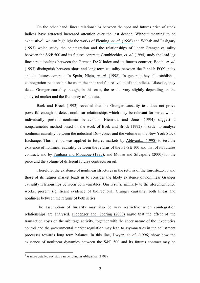
In order to tes the kind of temporal dependence which the analysed series present,

both linear and nonlinear temporal dependence tests will be used. The statistics of Ljung and

Box (1979) will be used for the first kind of dependence. This tests the null of the absence of

serial correlation with the statistics:

∑= −

+=k

1i

2

Tr

2)T(TQ(p)i

i , (1)

where T is the size of the sample and ri is the simple i-order correlation coefficient. In

this null (1) follows a distribution with k degrees of freedom2χ 2.

2 When this test is applied to the residuals of an ARMA(p,q) model, the degrees of freedom of the χ2 change to k-p-q.

4

The application of this test for a correlation order equalling 28 leads to the rejection

of the absence of correlation for spot returns. As for futures, the null is rejected at the 5%

significance level, but not at the 1%.

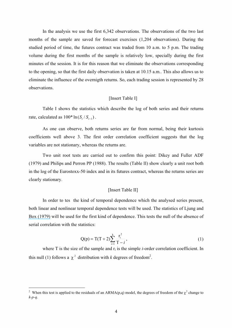
Two different tests, Q2 and BDS, will be used to test the presence of nonlinear

temporal dependence. The Q2 test was suggested by McLeod and Li (1983) to detect, among

others, nonlinear Garch structures. Given a temporal series xt (t=1,...,T), the statistics is:

∑= −

+=k

1i

22

TR

2)T(T(p)Qi

i , (2)

where and ∑∑−

=−

−

=

−−−=iT

ttit

iT

tti zxzxzxR

1

222

1

22 )(/)()( ∑=

=T

ttx

Tz

1

21 .

For the null of correlation absence, this statistics has a distribution with k degrees

of freedom

2χ3. The results of the application of this test to the returns series (Table III) show

clearly the presence of GARCH linear dependence.

As for the BDS test, it was suggested by Brock, Dechert and Scheinkman (1987) and

revised by Brock, Dechert, Scheinkman and LeBaron (1996). It allows to test when a

temporal series is independent and identically distributed (iid). It may be used to test whether

a model suits a specific temporal series, since it detects any structure in the error term, be it

linear, nonlinear or chaotic.

Given the temporal series xt (t=1,...,T), they are considered segments of the same

size, called M-stories and defined as: , where M is the

dimension. From these M-stories, the integral correlation C

)x,,x,x,x()x( 1t2t1ttt ++++= mm …

m(l) of m dimension and l

distance is defined as:

,))(x,)(x(I)T)(1T(

2)(C1T

T, jmjiI

ilm mmmm

l ∑+−≤≤≤−+−

= (3)

where Il(.) is the indicator function:

.)(x,)x(if0)(x,)x(if1

))(x,)(x(I

≥

<=

lmmlmm

mmji

jijil

where ||.|| indicates the maximum norm. The BDS test for an m fix dimension, an l distance

and a T sample size is:

3 See previous footnote.

5

,)(

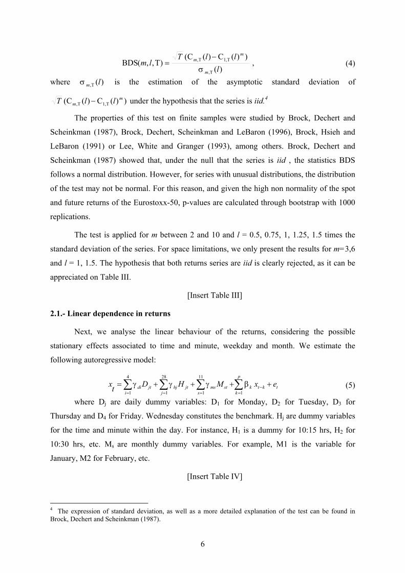
))(C)(C()T,,(BDS

T,

T,1T,

lllT

lmm

mm

σ

−= (4)

where is the estimation of the asymptotic standard deviation of )(T, lmσ

))(C( T,m

m lT C)( ,1T l − under the hypothesis that the series is iid.4

The properties of this test on finite samples were studied by Brock, Dechert and

Scheinkman (1987), Brock, Dechert, Scheinkman and LeBaron (1996), Brock, Hsieh and

LeBaron (1991) or Lee, White and Granger (1993), among others. Brock, Dechert and

Scheinkman (1987) showed that, under the null that the series is iid , the statistics BDS

follows a normal distribution. However, for series with unusual distributions, the distribution

of the test may not be normal. For this reason, and given the high non normality of the spot

and future returns of the Eurostoxx-50, p-values are calculated through bootstrap with 1000

replications.

The test is applied for m between 2 and 10 and l = 0.5, 0.75, 1, 1.25, 1.5 times the

standard deviation of the series. For space limitations, we only present the results for m=3,6

and l = 1, 1.5. The hypothesis that both returns series are iid is clearly rejected, as it can be

appreciated on Table III.

[Insert Table III]

2.1.- Linear dependence in returns

Next, we analyse the linear behaviour of the returns, considering the possible

stationary effects associated to time and minute, weekday and month. We estimate the

following autoregressive model:

4 28 11

1 1 1 1

p

di jt hj jt ms st k t k ti j s k

x D H M xt γ γ γ β −= = = =

= + + +∑ ∑ ∑ ∑ e+

(5)

where Dj are daily dummy variables: D1 for Monday, D2 for Tuesday, D3 for

Thursday and D4 for Friday. Wednesday constitutes the benchmark. Hj are dummy variables

for the time and minute within the day. For instance, H1 is a dummy for 10:15 hrs, H2 for

10:30 hrs, etc. Ms are monthly dummy variables. For example, M1 is the variable for

January, M2 for February, etc.

[Insert Table IV]

4 The expression of standard deviation, as well as a more detailed explanation of the test can be found in Brock, Dechert and Scheinkman (1987).

6

For the estimation of the models, we use the variance-covariance matrix suggested by

Newey and West (1987, 1994) to prevent the effect of possible heteroskedasticity and

residual autocorrelation. Ten lags are used for their estimation. The results obtained in the

estimation (Table IV) can be summarised as follows:

After a first estimation, we decided to eliminate the monthly dummy variables for not

being significant.

Not every day has a significant effect5. For both markets, the returns are significantly

lower on Tuesdays. As for the spot market, the returns seem to be higher on Mondays

(Fridays for futures).

In both markets, the returns are significantly negative between 15:45 hrs and 16:15

hrs and become significantly positive in the last half hour of the market6.

In both models, 12-order autoregressive structures are estimated. We opt to include

all the lags, regardless of their significance, so as to detect the complete linear behaviour of

both returns series.

Table V shows the diagnosis of temporal dependence in the residuals of the estimated

linear models. Both the Q(28) statistics and the LM test for 2-order autocorrelation indicate

that the existing linear structure in both returns series has been appropriately captured7.

[Insert Table V]

Nevertheless, the remaining applied tests indicate that the returns show nonlinear

temporal dependence. The Q2(28) and ARCH(5) tests [LM test to detect conditional

heteroskedasticity8, suggested by Engle(1982)] indicate that such nonlinearity may be

associated to nonlinear behaviours in variance.

To confirm this last point, we apply the third moment test, suggested by Hsieh

(1989). This tries to detect nonlinear behaviour in temporal series by exploiting the

difference between additive and multiplicative nonlinear dependence. The first of them

5 Daily dummy variables with a t-ratio over a unit remain in the model. 6 All intraday variables are included regardless of their significance. 7 The LM p-order autocorrelation test is calculated as TR2 of a regression of the model residuals on the explanatory variables and their p first lags. Under the no autocorrelation null, it is distributed as a χ2 with p degrees of freedom. 8 The ARCH-LM p-order test is calculated as TR2 of a regression of the squared model residuals on their p squared first lags Under the non conditional heteroskedasticity null, it is distributed as a χ2 with p degrees of freedom. If applied to the diagnosis of a GARCH model, it is calculated for the squared standardised residuals.

7

makes reference to the nonlinearity found in the mean of the process, whereas with the

second, that nonlinearity only enters through the variance

Starting from the filtered temporal series, ut, i.e., the residuals of the xt linear model,

the additive nonlinearity implies that 0)u,,u,x,,xu( 11 =−−−− kttktttE …… , whereas with

multiplicative nonlinearity 0)u,,u,x,,xu( 11 ≠−−−− kttktttE ……

),(uuu jiρ

. Hsieh (1989) defines

, which equals zero the null hypothesis of multiplicative

nonlinearity for every i . is estimated with:

3uuu /)uuu(),( ujtittEji σρ −−=

0, >j

2/32tuuu u),(

T

1uuu

T

1

∑

∑= −− /jtittjir , (6)

which is asymptotically distributed under the null as a zero mean normal and ω variance. The asymptotic test statistic is

6u/),( σji

9:

,),(

3 uuu

uuur

jirTMT

σ= (7)

where σ is an estimation consisting in ( ) . uuur

2/16u/),( σω ji

Table VI shows the results obtained applying this test to the residuals of the

previously estimated linear models. The statistics is calculated for i, j values between 1 and

5. As it can be observed, the null hypothesis of multiplicative nonlinearity is not rejected in

any case, what seems to indicate that the nonlinear dependence found may be due to the

presence of conditional heteroskedasticity in the series.

[Insert Table VI]

2.2.- Models for the nonlinear dependence of the returns

Given the results obtained, the following objective is to model the nonlinear

behaviour detected in the series through GARCH models. Starting from the AR specification

for the returns of the previous section, the residuals of both models are analysed to identify

the most suitable GARCH structure10, after which we decide to estimate the GJR-

GARCH(1,1) model, suggested by Glosten et al. (1993). This allows to detect asymmetrical

effects on the variance11. The final specification of the estimated models is:

9 For more detailed information about this test see Hsieh (1989). 10 Besides the ARCH-LM and Q2(28) tests, presented in the previous section, we also apply the test suggested by Engle and NG (1993) to detect the leverage effect on volatility, as well as the simple and partial autocorrelation functions of the squared residuals of the AR model. 11 The volatility reaction is higher when against negative rather than positive surprises.

8

),0(~,xMHDx 24

1

28

1 1

11

1t

i jt

p

ktktk

sstmsjthjitdit hNee∑ ∑ ∑∑

= = =−

=

++++= βγγγ (8)

∑∑∑===

−−− +++++=11

1

11

1

4

1

211

21

-1-t

2110

2t MHDS

sstms

sjthj

sitdittt heeh γγγβδαα , (9)

where S-t is a dummy variable that takes the value of 1 when the residual in t is

negative and zero for another case. Variables Di, Hj and Ms are the dummies defined in the

previous section. These variables allow to consider possible day-of-the-week effects and

month effects on the variance. Additionally, the intraday dummies are included to detect any

possible behavioural U-shaped type patterns in the volatility.

[Insert Table VII]

The results obtained are shown on Table VII. For space limitations, we only present

the model for the variance since the mean model shows few differences with the models

estimated in the previous section. Given the high nonlinearity of the residuals, we opt to use

the variance-covariance matrix, suggested by Bollerslev and Wooldrige (1992) and robust to

non normality problems. Both models are estimated through maximum likelihood, using the

BHHH algorithm by Bernd, et al. (1974). The main results can be summarised in the

following aspects:

After an initial estimation, it was decided to eliminate those dummies which proved

insignificant in the variance model, since their presence in it slows down the convergence of

the estimation algorithm.

An asymmetrical effect is to be found in both models, though higher for the spot

market. The response of the volatility to bad news is five times higher than the effect of good

news in the spot market, and about three times higher in the futures market.

For the spot, the volatility persistence degree, calculated as α + , is higher (0.89

against 0.62 in the futures). This result implies that the volatility has the property of mean

reversion, more pronounced in the futures market.

11 β

The variance level seems to be higher on Thursdays in the spot market, whereas on

Mondays it drops significantly in the futures market. Volatility follows a U-shaped type

behaviour in both models, with significantly higher volatility levels at the start and end of

the session, and generally lower ones in the intervening hours.

9

The effects associated to the month are significant in the variance, whereas none are

found in the mean model. January, February and December show higher volatility levels,

while this volatility drops significantly in the intervening months.

Table VIII shows the diagnosis of the temporal dependence in the residuals of the

estimated GARCH models. The Q(28) test confirms that the linear behaviour of both series

has been appropriately captured. The remaining tests are calculated on the standarized

residuals. The Q2(28) and ARCH(1) and ARCH(10) tests indicate the presence of nonlinear

temporal dependence in the standarized residual of the spot returns model, but not in the

futures model.

[Insert Table VIII]

The results of the BDS test indicate that the standarized residuals of both models are

not iid at the 5% of significance, although those of the spot GARCH model do seem to be iid

at the 1%, when the dimension is given value 312. With a 6 dimension, the rejection of the

null becomes clearer.

Finally, the results of the third moment test (Table IX) indicate that, except for some

i,j pairs, the null of multiplicative nonlinearity is rejected in both markets, with a stronger

rejection in the spot series than in the futures series. All of this implies the existence of

residual multiplicative nonlinear dynamic which has not been detected with the estimated

GARCH models. A possible explanation of this result may be found in the existence of

nonlinear relationships between both series. This dynamic, which has not been taken into

account in their individual analysis, is introduced in the next section.

[Insert Table IX]

3.- DYNAMIS BETWEEN THE INDEX AND ITS FUTURES CONTRACT

We now study the dynamic behaviour of the Eurostoxx-50 stock index and that of its

futures market as a whole. First, in our cointegration analysis, we allow the ECM, which

eliminates the deviations of the variables from their position of long term balance, to follow

a nonlinear adjustment process in the short term equations. This is possible applying the first

order Fourier approach, suggested by Ludlow and Enders (2000). Secondly, besides studying

the relationships of Linear Granger causality between the returns of both variables, we test

12 It is remarkable that the null cannot be rejected for a 2 dimension, regardless of the value of l in any of the markets.

10

the existence of nonlinear causality relationships using the contrast suggested by Hiemstra

and Jones (1994).

3.1.- Cointegration Analysis and Short Term Equations

Enders and Ludlow (2000) develop a technique that allows to test the existence of

cointegration without having to specify the kind of nonlinear adjustment to the long term

balance deviations13. These authors suggest an modification of the cointegration test of

Engle and Granger (1987), allowing long term balance deviations to follow this kind of

nonlinear process:

1

11

( )p

t t i t ii

e t e eα γ−

− −=

= + ∆∑ tε+ (10)

No specification of the functional form of α is required, since this can be

approximated by a sufficiently long Fourier series. Enders and Ludlow (2000) suggest:

( )t

0 1 12 2 ( ) sen cosk kt a a t b

T Tπ π

α = + + t (11)

where: k is a round number of the T/2 interval.

The key lies in that using equation (10), rather than determining a certain kind of

specific nonlinear adjustment, the problem is reduced to finding the most suitable values of

a0, a1, b1, k.14 These authors prove that the sufficient and necessary condition for the

adjustment process not to be explosive, or, in other words, for the variables to be

cointegrated is:

| a0 | < 1 + r2 / 4 for r ≤ 2 r a b= +1

212 (12)

The cointegration test with nonlinear adjustment is carried out in two stages: In the

first stage, we estimate the long term relationship between those variables capable of being

cointegrated, which are the value of the Eurostoxx-50 index and the price of its futures

contract in our analysis. The results are:

tF̂ = 0.19 + 0.98 Ct (32.81) (1356.02)

(13)

where: Ft is the futures price; Ct is the index value; t statistics in brackets.

13 Enders and Ludlow (2000) extend the work of Ludlow and Enders (2000) on ARMA estimation with Fourier coefficients, treating cointegration relationships explicitly. 14 The test of Engle and Granger (1987) is the specific case of a1, b1 equalling zero.

11

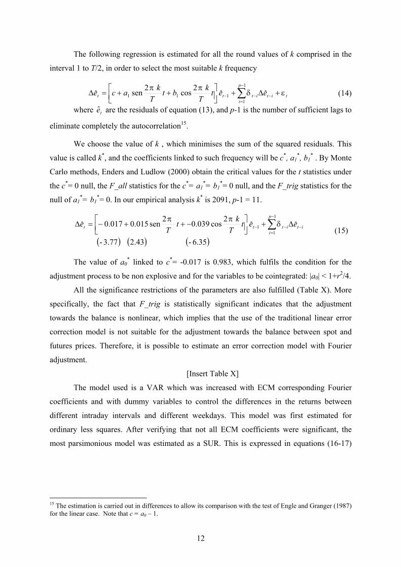
The following regression is estimated for all the round values of k comprised in the

interval 1 to T/2, in order to select the most suitable k frequency

t

p

iitittt eet

Tkbt

Tkace εδ

ππ+∆+

++=∆ ∑

−

=−−−

1

1111 ˆˆ

2cos 2sen ˆ (14)

where are the residuals of equation (13), and p-1 is the number of sufficient lags to

eliminate completely the autocorrelation

et

15.

We choose the value of k , which minimises the sum of the squared residuals. This

value is called k*, and the coefficients linked to such frequency will be c*, a1*, b1

* . By Monte

Carlo methods, Enders and Ludlow (2000) obtain the critical values for the t statistics under

the c*= 0 null, the F_all statistics for the c*= a1*= b1

*= 0 null, and the F_trig statistics for the

null of a1*= b1

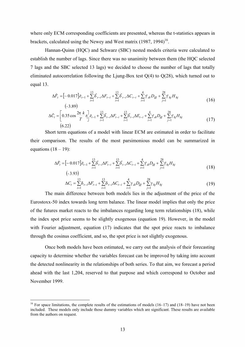
*= 0. In our empirical analysis k* is 2091, p-1 = 11.

( ) ( ) ( )6.35- 2.43 3.77-

ˆˆ 2cos 039.0 2sen 015.0017.0ˆ

1

11 ∑

−

=−−− ∆+

−++−=∆

p

iitittt eet

Tkt

Te δ

ππ (15)

The value of a0

* linked to c*= -0.017 is 0.983, which fulfils the condition for the

adjustment process to be non explosive and for the variables to be cointegrated: |a0| < 1+r2/4.

All the significance restrictions of the parameters are also fulfilled (Table X). More

specifically, the fact that F_trig is statistically significant indicates that the adjustment

towards the balance is nonlinear, which implies that the use of the traditional linear error

correction model is not suitable for the adjustment towards the balance between spot and

futures prices. Therefore, it is possible to estimate an error correction model with Fourier

adjustment.

[Insert Table X]

The model used is a VAR which was increased with ECM corresponding Fourier

coefficients and with dummy variables to control the differences in the returns between

different intraday intervals and different weekdays. This model was first estimated for

ordinary less squares. After verifying that not all ECM coefficients were significant, the

most parsimonious model was estimated as a SUR. This is expressed in equations (16-17)

15 The estimation is carried out in differences to allow its comparison with the test of Engle and Granger (1987) for the linear case. Note that c = a0 – 1.

12

where only ECM corresponding coefficients are presented, whereas the t-statistics appears in

brackets, calculated using the Newey and West matrix (1987, 1994)16.

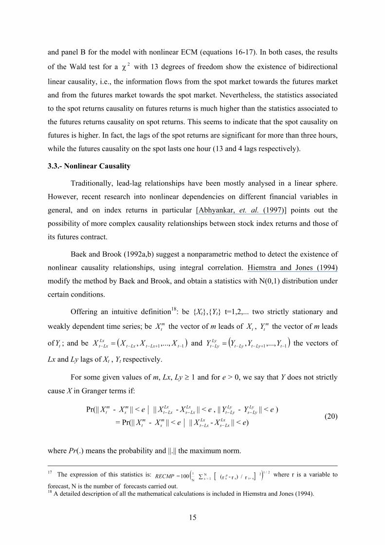
Hannan-Quinn (HQC) and Schwarz (SBC) nested models criteria were calculated to

establish the number of lags. Since there was no unanimity between them (the HQC selected

7 lags and the SBC selected 13 lags) we decided to choose the number of lags that totally

eliminated autocorrelation following the Ljung-Box test Q(4) to Q(28), which turned out to

equal 13.

[ ]

( ) 3.89-

ˆˆˆˆˆ 017.0ˆ28

1

4

1

13

1

13

11 ∑∑∑∑

===−−

=−−− ++∆+∆+−=∆

jhjhj

idi

iitit

iitittt HitDCFeF γγδδ

(16)

( ) 6.22

ˆˆˆˆˆ 2cos 35.0ˆ

28

1

4

1

13

1

13

11 ∑∑∑∑

===−−

=−−− ++∆+∆+

=∆

jhjhj

idi

iitit

iitittt HitDEFet

TkC γγδδ

π (17)

Short term equations of a model with linear ECM are estimated in order to facilitate

their comparison. The results of the most parsimonious model can be summarized in

equations (18 – 19):

[ ]

( ) 3.93-

ˆˆˆˆˆ 017.0ˆ28

1

4

1

13

1

13

11 ∑∑∑∑

===−−

=−−− ++∆+∆+−=∆

jhjhj

idi

iitit

iitittt HitDCFeF γγδδ

(18)

28

1

4

1

13

1

13

1∑∑∑∑===

−−=

−− ++∆+∆=∆j

hjhji

dii

ititi

ititt HitDCFC γγδδ (19)

The main difference between both models lies in the adjustment of the price of the

Eurostoxx-50 index towards long term balance. The linear model implies that only the price

of the futures market reacts to the imbalances regarding long term relationships (18), while

the index spot price seems to be slightly exogenous (equation 19). However, in the model

with Fourier adjustment, equation (17) indicates that the spot price reacts to imbalance

through the cosinus coefficient, and so, the spot price is not slightly exogenous.

Once both models have been estimated, we carry out the analysis of their forecasting

capacity to determine whether the variables forecast can be improved by taking into account

the detected nonlinearity in the relationships of both series. To that aim, we forecast a period

ahead with the last 1,204, reserved to that purpose and which correspond to October and

November 1999.

16 For space limitations, the complete results of the estimations of models (16–17) and (18–19) have not been included. These models only include those dummy variables which are significant. These results are available from the authors on request.

13

We calculate the mean squared error in percentages (RECMP)17 to compare the

forecasting capacity. The results of this analysis indicate that, as far as forecast is concerned,

this does not improve, being the RECMP of both models identical. (0.1844 for spot and

0.2014 for futures).

3.2.- Linear Causality

When two or more variables are cointegrated, it is necessary to distinguish between

short and long term Granger causality. Long term causality [Granger 1986)] is the result of

including all variables lagged by one period in the ECM. This causality will always occur at

least in one direction since, according to Granger representation theorem, if two variables are

cointegrated, at least one of them must respond to the deviations of the long term balance

relationship. In other words, the ECM must be significant in, at least, one of both short term

equations. Long term causality will be linear when the ECM is linear and nonlinear should

the ECM include any nonlinear expression.

In the case of the Eurostoxx-50, the index value causes its futures contract returns

linearly in the long term, since the index enters linearly in the ECM of the futures returns

equation (equation 16). On the other hand, the price of the futures contract causes the long

term index returns nonlinearly, since the coefficient associated to the cosinus in the ECM of

the index returns equation is significant. (equation 17).

Linear Granger causality (1969), also known as short term linear causality, analyses

the temporal information flows in a linear context. Using a more formal definition, a variable

is said to cause another, if the introduction of the lags of the causal variable in the model of

the caused variable improves the forecast of the caused variable.

To test the existence of short term causality, we start from a VAR model and carry

out a combined significance test of the lags of the causal variable in the equation of the

caused variable. The null to test “X does not cause Y in the short term”, is equivalent to

testing that the coefficients associated to the lags of Y in the equation of X equal zero.

[Insert Table XI]

Table XI shows the results of the short term linear causality tests for both models

estimated in the previous section: panel A for the model with linear ECM (equations 18-19),

14

and panel B for the model with nonlinear ECM (equations 16-17). In both cases, the results

of the Wald test for a with 13 degrees of freedom show the existence of bidirectional

linear causality, i.e., the information flows from the spot market towards the futures market

and from the futures market towards the spot market. Nevertheless, the statistics associated

to the spot returns causality on futures returns is much higher than the statistics associated to

the futures returns causality on spot returns. This seems to indicate that the spot causality on

futures is higher. In fact, the lags of the spot returns are significant for more than three hours,

while the futures causality on the spot lasts one hour (13 and 4 lags respectively).

2χ

3.3.- Nonlinear Causality

Traditionally, lead-lag relationships have been mostly analysed in a linear sphere.

However, recent research into nonlinear dependencies on different financial variables in

general, and on index returns in particular [Abhyankar, et. al. (1997)] points out the

possibility of more complex causality relationships between stock index returns and those of

its futures contract.

Baek and Brook (1992a,b) suggest a nonparametric method to detect the existence of

nonlinear causality relationships, using integral correlation. Hiemstra and Jones (1994)

modify the method by Baek and Brook, and obtain a statistics with N(0,1) distribution under

certain conditions.

Offering an intuitive definition18: be {Xt},{Yt} t=1,2,... two strictly stationary and

weakly dependent time series; be the vector of m leads of , the vector of m leads

of ; and be and

Xtm

1 ,...,+Lx

Xt Ytm

Yt ( )1, −−−− = ttLxtLx

Lxt XXXX ( )1−−− = tLytLy

Lyt YY 1 ,...,+Ly, −tYY the vectors of

Lx and Ly lags of Xt , Yt respectively.

For some given values of m, Lx, Ly ≥ 1 and for e > 0, we say that Y does not strictly

cause X in Granger terms if:

Pr(|| - || < e Xtm Xs

m || - || < e , || - || < e ) Xt LxLx− Xs Lx

Lx− Yt Ly

Ly− Ys Ly

Ly−

= Pr(|| - || < e Xtm Xs

m || - || < e) Lxt LxX − Xs Lx

Lx−

(20)

where Pr(.) means the probability and ||.|| the maximum norm.

17 The expression of this statistics is: RECMP where r is a variable to

forecast, N is the number of forecasts carried out. [ ]( )r / )r - r( 100 = st+ss

2 N1=sN

1 2/1p∑

18 A detailed description of all the mathematical calculations is included in Hiemstra and Jones (1994).

15

The modified causality test by Baek and Brook determines whether the conditional

probability that two arbitrary vectors of m length remain within an e distance (given that the

corresponding vectors of Lx lags are within that distance) is influenced by the corresponding

lags vector Ly. In other words, testing if the lagged values of Y are capable of forecasting the

present value of X.

In practice, expression (20) is implemented using integral correlation. This ‘counts’

the number of times that both vectors are one within a specific distance of the other.

Hiemstra and Jones (1994) argue that a positive and significant value of the statistics

suggests that the lagged values of Y help to forecast X, whereas a negative and significant

value of the statistics suggests that the knowledge of the lagged values of Y blurs the forecast

of X. For this reason, they maintain that the critical values corresponding to a right-tail must

be used.

Besides, Hiemstra and Jones (1994) argue that, when carrying out the nonlinear

Granger causality test between two variables, it is advisable to eliminate the possible linear

forecasting power of the variables by means of a VAR model. In this way, any increase in

the forecasting power of a residuals series on the other can be regarded as nonlinear

forecasting power. For this reason, in our empirical analysis of the nonlinear causality test

between the returns of the Eurostoxx-50 and those of its futures market, we have used the

standarized residuals of the VAR models estimated in section 3.1 (equations 16-17 and 18-

19)19.

The modified Baek and Brook test requires from the researcher to choose the m lead

values, the Lx Ly lags and the scale parameter e. Since no references are made in the existing

literature on how to select the optimum values, we follow Hiemstra and Jones (1994), and

fix m = 1, e = 1.5 times the standard deviation (equalling 1 in this case, as they are

standarized series) and the same number of lags for both series so that Lx=Ly takes values

between 1 and 10, which allows us to test the existence of nonlinear causality during a

maximum interval of two and a half hours20.

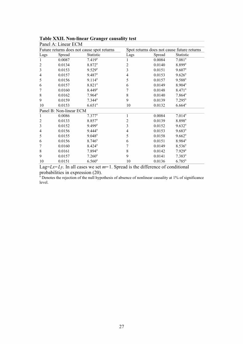
[Insert Table XII]

Table XII shows the results of the modified Baek and Brook test, applied to the

residuals of the VAR models corresponding to the returns of the Eurostoxx-50 index and the

19 Linear causality tests on these residuals confirm the absence of causality between both series. 20 It was also calculated for e=1 and e = 0.5, obtaining similar results.

16

returns of its futures contract: panel A for the model with linear ECM (equations 18-19) and

panel B for the model with nonlinear ECM (equations 16-17). Unanimously, and regardless

of the path taken in the adjustment of imbalances regarding the long term relationship, all

statistics indicate the existence of bidirectional short term nonlinear causality between the

returns of both markets. This result is repeated for all the lags considered. None of the

normalized statistics is below 6.56, which seems to be a very strong piece of evidence in

favour of the existence of nonlinear causality in both directions.

For short term nonlinear causality, we cannot observe that either market leads the

other, unlike the results for linear causality. These results agree with those obtained by

Abhyankar (1998) for the FT-SE 100 index and its futures market.

4.- CONCLUSIONS

The main objective of this study has been to analyse the individual and combined

behaviour of the Eurostoxx-50 and its futures contract. It has become evident that nonlinear

dynamics exist in the returns which cannot solely be explained by the presence of

conditional heteroskedasticity.

First of all, we carried out a BDS test both on the returns series linearly filtered

considering intraday stationarities, weekday and month, and on the returns series filtered by

GARCH effects. The results of such tests indicate that the variables are not iid in both cases

This result coincides with the existing literature on the behaviour of several financial series.

As for the dynamic analysis of the relationships between spot and futures markets,

we highlight the existence of cointegration between the prices of the Eurostoxx 50 and its

futures contract. Following Enders and Ludlow (2000), we have proved that the adjustment

process is nonlinear in the model of the adjustments against imbalances in the long term

relationship. The results of this model show that the traditional linear ECM, more restrictive

that the Fourier adjustment, is not more suitable as, in this case, the spot price seems to be a

slightly exogenous variable, whereas the use of a more flexible Fourier adjustment

demonstrates that the spot price responds to imbalance by means of the cosinus coefficient.

This result indicates that the model with linear ECM fails to explain the adjustment process

of both markets in all its complexity.

17

Finally, in the study of causal relationships, and following Hiemstra and Jones

(1994), we distinguish between linear and nonlinear Granger causality, establishing that the

information flows are bidirectional both in the linear and in the nonlinear sphere.

Remarkably, as for short term nonlinear causality, neither market seems to lead the other

which could be due to the low levels of futures volume due to the youth of the futures

contract. These results as a whole prove the importance of considering the existence of

nonlinear relationships between the financial variables studied. Nevertheless, we are aware

that the econometric tests applied show the existence of nonlinear dynamics empirically but

fail to explain theoretically and formally the nature of such dynamics.

18

REFERENCES Abhyankar, A. (1998): “Linear and nonlinear Granger causality: Evidence from the UK

stock index futures market”, The Journal of Futures Market, 18: 519-540.

Abhyankar, A. (1992): , “A nonparametric test for independence of multivariate time series”, Statistica Sinica, 2: 137-156.

Abhyankar, A.; Copeland, L. S.; Wong, W. (1997): “Uncovering nonlinear structure in real-time stock market indexes: The S&P 500, the DAX, the Nikkei 225 and the FT-SE 100”, Journal of Business Economics and Statistics, 15: 1-14.

Baek, E.; Brook, W. (1992): “A general test for nonlinear Granger causality: Bivariate model”, Working Paper, Iowa State Unversity and University of Wisconsin, Madison

Balke, N. S.; Fomby, T. B. (1997): “Threshold cointegration”, International Economic Review, 38: 627-645.

Berndt, E. K.; Hall, B. H.; Hall, R. E.; Haussman, J. A. (1974): “ Estimation and inference in nonlinear structure models”, Annals of Economic and Social Measurement, 4: 653-665.

Blasco, N.; Santamaria, R. (1996): “Testing memory patterns in the Spanis stock market”, Applied Financial Economics, 6: 401-411.

Bollerslev, T.; Wooldridge J. M. (1992): “Quasi-Maximum likelihood estimation and inference in dynamic models with time varying covariances”, Econometric Reviews, 11: 143-172.

Booth, G. G.; Martikainen, T.; Puttonen, V. (1993): “The international lead-lag effect between market returns: Comparison of stock index futures and cash markets”, Journal of International Financial Markets, Institutions and Money, 3: 59-71.

Brock, W. A.; Hsieh, D. A.; LeBaron, B. (1991): Nonlinear dynamics, chaos and instability, Cambridge, MA: The MIT press.

Brock, W., W. Dechert and J. Scheinkman, (1987) “A test for independence based on the correlation dimension”, Working Paper, University of Wisconsin at Madison, University of Houston, and University of Chicago.

Brock, W.; Dechert, D.; Sheinkman, J.; LeBaron, B. (1996): “A test for independence based on the correlation dimension” Econometric Reviews, 15: 197-235.

Dickey, D A; Fuller W A (1979): “Distribution of the estimators for autoregressive time series with a unit root”, Journal of the American Statistical Association, 74: 427-431.

Dwyer, G. P.; Locke, P.; Yu, W. (1996): “Index arbitrage and nonlinear dynamics between the S&P500 futures and cash”, Review of Financial Studies, 9: 353-387.

Enders, W.; Granger, C.W. (1998): “Unit root test and asymmetric adjustment with an exemple using the term structure of interest rates”, Journal of Business and Economic Statistics, 16: 304-311.

Enders, W.; Loudlow, J. (2000): “Non-linear decay: Tests for an attractor using a Fourier approximation”, Iowa State University, (Mimeo)

Enders. W.; Silkos, P. L. (2001): “Cointegration and threshold adjustment”, Journal of Business and Economic and Statistics, 19: 166-176.

19

Engle, R. F. (1982): “Autoregressive conditional heteroskedasticity with estimates of the variance of U.K. inflation”, Econometrica, 50: 987-1008.

Engle, R. F.; Granger, C. W. J. (1987): “Cointegration and error correction: Representation, estimation and testing”, Econometrica, 55: 251-276.

Engle, R. F.; Ng V. K. (1993): “Measuring and testing the impact of news on volatility”, Journal of Finance, 48: 1022-1082.

Fleming, J.; Ostdiek, B: ; Whaley, R. (1996): “Trading costs and the relative rates of price discovery in stock, futures and option markets”, The Journal of Futures Markets, 16: 353-387.

Fujihara, R.; Mougoue, M. (1997): “An examination of linear and nonlinear causal relationships betwenn price variability and volume in petroleum futures markets”, Journal of Futures Markets, 17: 385-416.

Gao, A. H.; Wang, G. H. K. (1999):“Modelling non linear dynamics of daily futures prices change”, The Journal of Futures Markets, 19: 325-351.

Glosten, L. R.; Jaganathan, R.; Runkle, D. (1993): “On the relation between the expected value and the volatility of the normal excess return on stocks”, Journal of Finance, 48: 1779-1801.

Granger , C. W. J. (1969): “Investigating causal relations by econometric models and cross-spectral methods”, Econometrica, 37: 424-438.

Granger , C. W. J. (1986): “Some recent developments in a concept of causality”, Journal of Econometrics, 39: 199-211.

Grunbichler, A.; Longstaff, F.; West, E. (1987): “Electronic screen trading and the transmission of information: An empirical examination”, Journal of Financial Intermediation, 3: 166-187.

Hiemstra, C.; Jones, J. D. (1994): “Testing for linear and nonlinear Granger causality in the stock price-volume relation”, The Journal of Finance, 49 (5): 1639-1664.

Hsieh, D. A. (1989): “Testing for nonlinear dependence in daily foreign exchange rate”, Journal of Business, 62: 339-368.

Hsieh, D. A. (1991), “Chaos and nonlinear dynamics: Application to financial markets” Journal of Finance, 46: 1839-1876.

Hsieh, D. A. (1993), “Implications of nonlinear dynamics of financial risk management”, Journal of Finance and Quantitative Analysis, 28: 41-64.

Lee, T.; White, H.; Granger, C. (1993): “Testing for neglected nonlinearity in time series models: A comparison of neural network method and alternative tests” Journal of Econometrics, 56: 269-290.

Ljung, G.; Box, G. (1979): “On a measure of lack of fit in time series models” Biometrika, 66: 265-270.

Ludlow, J.; Enders, W. (2000): “Estimating non-linear ARMA models using a Fourier coefficients”, International Journal of Forecasting, 16: 333-347.

MacKinnon, J. G. (1991): “Critical values for cointegration tests” en Long-run Economic Relationships: Readings in Cointegration, editado por R F Engle y C W J Granger, Oxford University Press.

20

McLeod, A I; Li, W K (1983).”Diagnostic checking ARMA time series models using squared-residual autocorrelations” Journal of Time Series Analysis, 4: 269-273.

Mossa, I. A.; Silvapulle, P. (2000): “The price-volume relationship in the crude oil futures market: Some results based on linear and nonlinear causality testing”, International Review of Economics and Finance, 9: 11-30.

Newey, W.; West, K. (1987): “Hypothesis testing with efficient method of moments estimation”, International Economic Review, 28: 777-787.

Newey, W.; West, K. (1994): “Automatic lag selection in covariance matrix estimation”, Review of Economic Studies, 61: 631-653.

Nieto, L.; Fernández, A; Muñoz, M.J. (1998): “Market efficiency in the Spanish derivatives markets: An empirical analysis”, International Advances in Economic Research, 4: 349-355.

Phillips, P. C. B.; Perron, P. (1988): “Testing for a unit root in time series regression”, Biometrika, 75: 335-346.

Pippenger, M. K.; Goering, G. E. (2000): “Additional results on the power of unit root and cointegration tests under threshold processes”, Applied Economic Letters¸7: 641-644.

Savit, R. (1988): “When random is not random: An introduction to chaos in market prices”, Journal of Futures Markets, 8: 271-290.

Wahab, M.; Lashigari, M. (1993): “Price discovery and error correction in stock index and stock index futures markets: A cointegration approach”, The Journal of Futures Markets, 13: 711-42.

Yang, S. R.; Brorsen, B. W. (1993):“Nonlinear dynamics of daily futures prices: conditional heteroskedasticity or chaos?”, The Journal of Futures Markets, 13: 175-191.

Yang, S. R.; Brorsen, B. W. (1994):“Daily futures price changes and nonlinear dynamics”, Structural Change and Economic Dynamics, 5: 111-132.

21

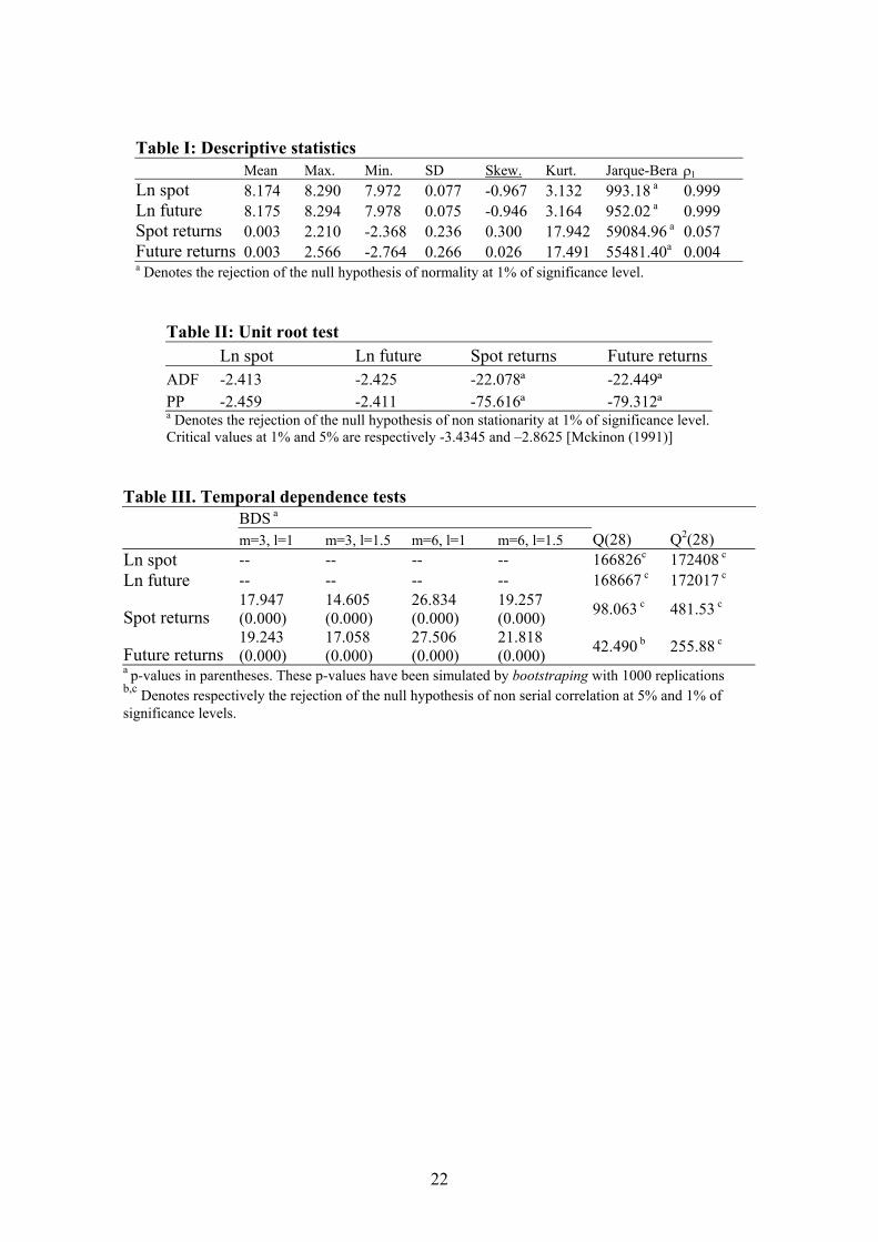
Table I: Descriptive statistics Mean Max. Min. SD Skew. Kurt. Jarque-Bera ρ1 Ln spot 8.174 8.290 7.972 0.077 -0.967 3.132 993.18 a 0.999 Ln future 8.175 8.294 7.978 0.075 -0.946 3.164 952.02 a 0.999 Spot returns 0.003 2.210 -2.368 0.236 0.300 17.942 59084.96 a 0.057 Future returns 0.003 2.566 -2.764 0.266 0.026 17.491 55481.40a 0.004 a Denotes the rejection of the null hypothesis of normality at 1% of significance level.

Table II: Unit root test Ln spot Ln future Spot returns Future returns ADF -2.413 -2.425 -22.078ª -22.449ª PP -2.459 -2.411 -75.616ª -79.312ª a Denotes the rejection of the null hypothesis of non stationarity at 1% of significance level. Critical values at 1% and 5% are respectively -3.4345 and –2.8625 [Mckinon (1991)]

Table III. Temporal dependence tests BDS a m=3, l=1 m=3, l=1.5 m=6, l=1 m=6, l=1.5 Q(28) Q2(28) Ln spot -- -- -- -- 166826c 172408 c Ln future -- -- -- -- 168667 c 172017 c

Spot returns 17.947 (0.000)

14.605 (0.000)

26.834 (0.000)

19.257 (0.000) 98.063 c 481.53 c

Future returns 19.243 (0.000)

17.058

(0.000) 27.506

(0.000) 21.818

(0.000) 42.490 b 255.88 c a p-values in parentheses. These p-values have been simulated by bootstraping with 1000 replications b,c Denotes respectively the rejection of the null hypothesis of non serial correlation at 5% and 1% of significance levels.

22

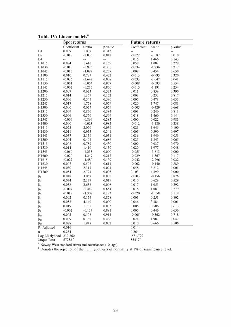
Table IV: Linear modelsa Spot returns Future returns Coefficient t-ratio p-value Coefficient t-ratio p-value D1 0.009 1.009 0.313 -- -- -- D2 -0.018 -2.036 0.042 -0.022 -2.587 0.010 D4 -- -- -- 0.015 1.466 0.143 H1015 0.074 1.410 0.159 0.058 1.082 0.279 H1030 -0.015 -0.926 0.355 -0.034 -1.236 0.217 H1045 -0.015 -1.087 0.277 0.008 0.454 0.650 H1100 0.010 0.787 0.432 -0.013 -0.995 0.320 H1115 -0.036 -2.642 0.008 -0.033 -2.047 0.041 H1130 -0.001 -0.054 0.957 -0.008 -0.593 0.554 H1145 -0.002 -0.215 0.830 -0.015 -1.191 0.234 H1200 0.007 0.623 0.533 0.011 0.859 0.390 H1215 0.014 1.367 0.172 0.003 0.232 0.817 H1230 0.006 0.545 0.586 0.005 0.478 0.633 H1245 0.017 1.758 0.079 0.020 1.747 0.081 H1300 0.000 0.027 0.979 -0.005 -0.429 0.668 H1315 0.009 0.870 0.384 0.003 0.240 0.811 H1330 0.006 0.570 0.569 0.018 1.460 0.144 H1345 -0.009 -0.869 0.385 0.000 0.022 0.983 H1400 0.000 -0.023 0.982 -0.012 -1.180 0.238 H1415 0.025 2.070 0.039 0.021 1.646 0.100 H1430 0.011 0.953 0.341 0.005 0.390 0.697 H1445 0.037 2.159 0.031 0.036 1.949 0.051 H1500 0.004 0.404 0.686 0.025 1.845 0.065 H1515 0.008 0.789 0.430 0.000 0.037 0.970 H1530 0.014 1.410 0.159 0.020 1.977 0.048 H1545 -0.060 -4.235 0.000 -0.055 -3.813 0.000 H1600 -0.020 -1.249 0.212 -0.029 -1.567 0.117 H1615 -0.027 -1.480 0.139 -0.042 -2.296 0.022 H1630 0.007 0.508 0.611 -0.002 -0.140 0.889 H1645 0.030 2.317 0.021 0.058 3.212 0.001 H1700 0.054 2.794 0.005 0.103 4.890 0.000 β1 0.048 3.067 0.002 -0.003 -0.156 0.876 β2 0.034 2.339 0.019 0.010 0.629 0.529 β3 0.038 2.636 0.008 0.017 1.055 0.292 β4 -0.007 -0.449 0.654 0.016 1.083 0.279 β5 -0.019 -1.302 0.193 -0.020 -1.558 0.119 β6 0.002 0.154 0.878 0.003 0.251 0.802 β7 0.052 4.140 0.000 0.046 3.384 0.001 β8 0.019 1.735 0.083 0.006 0.506 0.613 β9 -0.002 -0.137 0.891 0.006 0.446 0.656 β10 0.002 0.108 0.914 -0.005 -0.362 0.718 β11 0.009 0.730 0.466 0.024 1.987 0.047 β12 0.028 1.948 0.052 0.010 0.666 0.506 R2 Adjusted 0.016 0.014 σ 0.234 0.264 Log Likelyhood 230.260 -531.790 Jarque-Bera 57752 b 55417b a Newey-West standard errors and covariances (10 lags). b Denotes the rejection of the null hypothesis of normality at 1% of significance level.

23

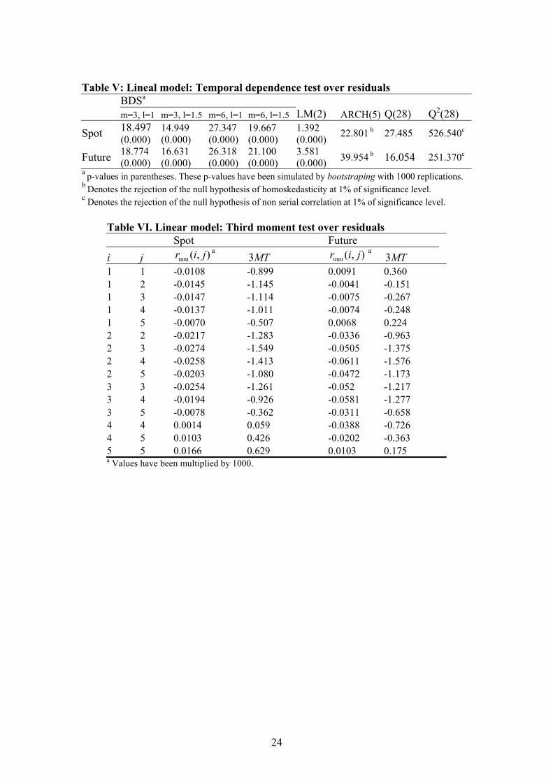
Table V: Lineal model: Temporal dependence test over residuals BDSa m=3, l=1 m=3, l=1.5 m=6, l=1 m=6, l=1.5 LM(2) ARCH(5) Q(28) Q2(28)

Spot 18.497 (0.000)

14.949 (0.000)

27.347 (0.000)

19.667 (0.000)

1.392 (0.000) 22.801 b 27.485 526.540c

Future 18.774 (0.000)

16.631 (0.000)

26.318 (0.000)

21.100 (0.000)

3.581 (0.000) 39.954 b 16.054 251.370c

a p-values in parentheses. These p-values have been simulated by bootstraping with 1000 replications. b Denotes the rejection of the null hypothesis of homoskedasticity at 1% of significance level. c Denotes the rejection of the null hypothesis of non serial correlation at 1% of significance level.

Table VI. Linear model: Third moment test over residuals Spot Future i j ),(uuu jir a MT3 ),(uuu jir a MT3 1 1 -0.0108 -0.899 0.0091 0.360 1 2 -0.0145 -1.145 -0.0041 -0.151 1 3 -0.0147 -1.114 -0.0075 -0.267 1 4 -0.0137 -1.011 -0.0074 -0.248 1 5 -0.0070 -0.507 0.0068 0.224 2 2 -0.0217 -1.283 -0.0336 -0.963 2 3 -0.0274 -1.549 -0.0505 -1.375 2 4 -0.0258 -1.413 -0.0611 -1.576 2 5 -0.0203 -1.080 -0.0472 -1.173 3 3 -0.0254 -1.261 -0.052 -1.217 3 4 -0.0194 -0.926 -0.0581 -1.277 3 5 -0.0078 -0.362 -0.0311 -0.658 4 4 0.0014 0.059 -0.0388 -0.726 4 5 0.0103 0.426 -0.0202 -0.363 5 5 0.0166 0.629 0.0103 0.175 a Values have been multiplied by 1000.

24

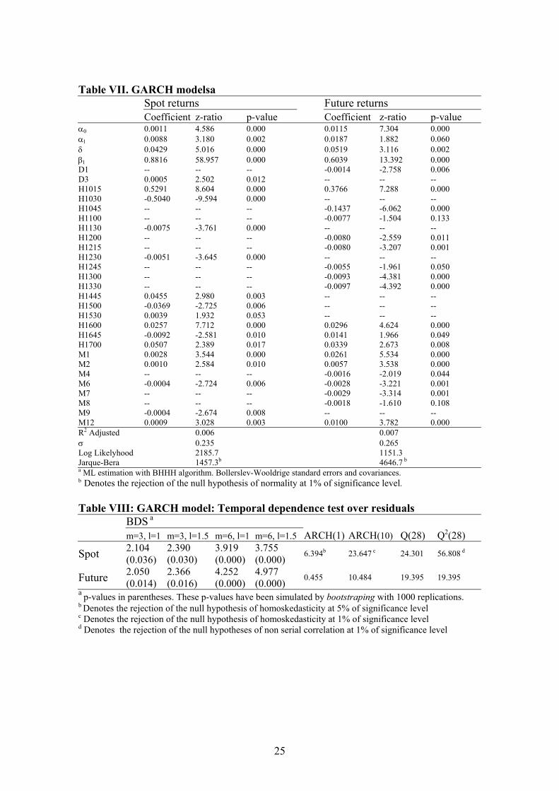
Table VII. GARCH modelsa Spot returns Future returns Coefficient z-ratio p-value Coefficient z-ratio p-value α0 0.0011 4.586 0.000 0.0115 7.304 0.000 α1 0.0088 3.180 0.002 0.0187 1.882 0.060 δ 0.0429 5.016 0.000 0.0519 3.116 0.002 β1 0.8816 58.957 0.000 0.6039 13.392 0.000 D1 -- -- -- -0.0014 -2.758 0.006 D3 0.0005 2.502 0.012 -- -- -- H1015 0.5291 8.604 0.000 0.3766 7.288 0.000 H1030 -0.5040 -9.594 0.000 -- -- -- H1045 -- -- -- -0.1437 -6.062 0.000 H1100 -- -- -- -0.0077 -1.504 0.133 H1130 -0.0075 -3.761 0.000 -- -- -- H1200 -- -- -- -0.0080 -2.559 0.011 H1215 -- -- -- -0.0080 -3.207 0.001 H1230 -0.0051 -3.645 0.000 -- -- -- H1245 -- -- -- -0.0055 -1.961 0.050 H1300 -- -- -- -0.0093 -4.381 0.000 H1330 -- -- -- -0.0097 -4.392 0.000 H1445 0.0455 2.980 0.003 -- -- -- H1500 -0.0369 -2.725 0.006 -- -- -- H1530 0.0039 1.932 0.053 -- -- -- H1600 0.0257 7.712 0.000 0.0296 4.624 0.000 H1645 -0.0092 -2.581 0.010 0.0141 1.966 0.049 H1700 0.0507 2.389 0.017 0.0339 2.673 0.008 M1 0.0028 3.544 0.000 0.0261 5.534 0.000 M2 0.0010 2.584 0.010 0.0057 3.538 0.000 M4 -- -- -- -0.0016 -2.019 0.044 M6 -0.0004 -2.724 0.006 -0.0028 -3.221 0.001 M7 -- -- -- -0.0029 -3.314 0.001 M8 -- -- -- -0.0018 -1.610 0.108 M9 -0.0004 -2.674 0.008 -- -- -- M12 0.0009 3.028 0.003 0.0100 3.782 0.000 R2 Adjusted 0.006 0.007 σ 0.235 0.265 Log Likelyhood 2185.7 1151.3 Jarque-Bera 1457.3b 4646.7 b a ML estimation with BHHH algorithm. Bollerslev-Wooldrige standard errors and covariances. b Denotes the rejection of the null hypothesis of normality at 1% of significance level.

Table VIII: GARCH model: Temporal dependence test over residuals BDS a m=3, l=1 m=3, l=1.5 m=6, l=1 m=6, l=1.5 ARCH(1) ARCH(10) Q(28) Q2(28)

Spot 2.104 (0.036)

2.390 (0.030)

3.919 (0.000)

3.755 (0.000) 6.394b 23.647 c 24.301 56.808 d

Future 2.050 (0.014)

2.366 (0.016)

4.252 (0.000)

4.977 (0.000) 0.455 10.484 19.395 19.395

a p-values in parentheses. These p-values have been simulated by bootstraping with 1000 replications. b Denotes the rejection of the null hypothesis of homoskedasticity at 5% of significance level c Denotes the rejection of the null hypothesis of homoskedasticity at 1% of significance level d Denotes the rejection of the null hypotheses of non serial correlation at 1% of significance level

25

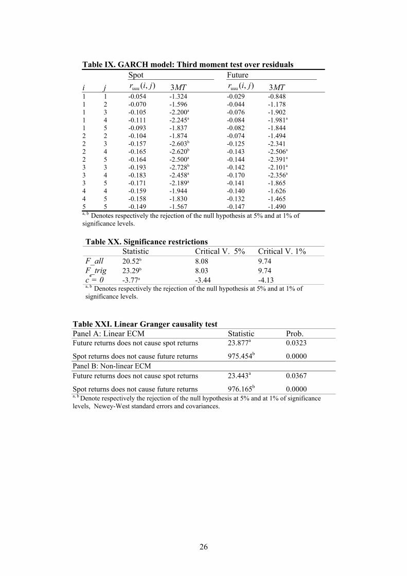
Table IX. GARCH model: Third moment test over residuals Spot Future i j ),(uuu jir MT3 ),(uuu jir MT3 1 1 -0.054 -1.324 -0.029 -0.848 1 2 -0.070 -1.596 -0.044 -1.178 1 3 -0.105 -2.200a -0.076 -1.902 1 4 -0.111 -2.245a -0.084 -1.981a 1 5 -0.093 -1.837 -0.082 -1.844 2 2 -0.104 -1.874 -0.074 -1.494 2 3 -0.157 -2.603b -0.125 -2.341 2 4 -0.165 -2.620b -0.143 -2.506a 2 5 -0.164 -2.500a -0.144 -2.391a 3 3 -0.193 -2.728b -0.142 -2.101a 3 4 -0.183 -2.458a -0.170 -2.356a 3 5 -0.171 -2.189a -0.141 -1.865 4 4 -0.159 -1.944 -0.140 -1.626 4 5 -0.158 -1.830 -0.132 -1.465 5 5 -0.149 -1.567 -0.147 -1.490 a, b Denotes respectively the rejection of the null hypothesis at 5% and at 1% of significance levels.

Table XX. Significance restrictions Statistic Critical V. 5% Critical V. 1% F_all 20.52b 8.08 9.74 F_trig 23.29b 8.03 9.74 c*= 0 -3.77a -3.44 -4.13 a, b Denotes respectively the rejection of the null hypothesis at 5% and at 1% of significance levels.

Table XXI. Linear Granger causality test Panel A: Linear ECM Statistic Prob. Future returns does not cause spot returns 23.877a 0.0323 Spot returns does not cause future returns 975.454b 0.0000 Panel B: Non-linear ECM Future returns does not cause spot returns 23.443a 0.0367 Spot returns does not cause future returns 976.165b 0.0000 a, b Denote respectively the rejection of the null hypothesis at 5% and at 1% of significance levels, Newey-West standard errors and covariances.

26

27

Table XXII. Non-linear Granger causality test Panel A: Linear ECM Future returns does not cause spot returns Spot returns does not cause future returns Lags Spread Statistic Lags Spread Statistic 1 0.0087 7.419a 1 0.0084 7.081a 2 0.0134 8.872a 2 0.0140 8.899a 3 0.0153 9.529a 3 0.0151 9.607a 4 0.0157 9.487a 4 0.0153 9.626a 5 0.0156 9.114a 5 0.0157 9.588a 6 0.0157 8.821a 6 0.0149 8.904a 7 0.0160 8.449a 7 0.0148 8.471a 8 0.0162 7.964a 8 0.0140 7.864a 9 0.0159 7.344a 9 0.0139 7.295a 10 0.0153 6.651a 10 0.0132 6.664a Panel B: Non-linear ECM 1 0.0086 7.377a 1 0.0084 7.014a 2 0.0133 8.857a 2 0.0139 8.898a 3 0.0152 9.499a 3 0.0152 9.632a 4 0.0156 9.444a 4 0.0153 9.683a 5 0.0155 9.048a 5 0.0158 9.662a 6 0.0156 8.746a 6 0.0151 8.984a 7 0.0160 8.424a 7 0.0149 8.536a 8 0.0161 7.894a 8 0.0142 7.929a 9 0.0157 7.260a 9 0.0141 7.383a 10 0.0151 6.560a 10 0.0136 6.785a Lag=Lx=Ly. In all cases we set m=1. Spread is the difference of conditional probabilities in expression (20). a Denotes the rejection of the null hypothesis of absence of nonlinear causality at 1% of significance level.