
Long-Lived Information and Intraday Patterns
28
Transcript of Long-Lived Information and Intraday Patterns

Long-Lived Information and Intraday Patterns�
Kerry Back
Olin School of Business
Washington University in St. Louis
St. Louis, MO 63130
Hal Pedersen
Faculty of Management
181 Freedman Crescent
University of Manitoba
Winnipeg, Manitoba R3T 5V4
CANADA
First draft: July, 1994
Current draft: July 17, 1995
�This paper comprised part of the second author's Ph.D. thesis at Washington Univer-
sity in St. Louis. He gratefully acknowledges support from a Society of Actuaries Ph.D.
Grant. We are grateful for numerous helpful comments from participants at seminars at
the University of Iowa, the University of Michigan, Vanderbilt University, Northwestern
University, and the Workshop on Mathematical Problems in Finance at the Institute for
Advanced Studies.

Long-Lived Information and Intraday Patterns
Abstract
This paper studies the e�ect of clustering of liquidity trades on intraday
patterns of volatility and market depth when private information is long-
lived. The assumption of long-lived information allows us to distinguish
between the patterns of information arrival and information use. Our results
are: (i) volatility follows the same pattern as liquidity trading, (ii) there are
no systematic patterns in the price impacts of orders, and (iii) the timing
of information arrival is is unimportant. Result (i) is the same as that
obtained by Admati and P eiderer (1988) in a model of short-lived private
information, but (ii) and (iii) are di�erent.

It is well documented that there are systematic intraday patterns in the
volatility of security prices and the volume of trading. In a widely cited
paper, Admati and P eiderer (1988) o�er an explanation of these patterns:
clustering in time of liquidity-motivated trades induces clustering of informa-
tion acquisition and informed trading, which generates the same clustering
of information-driven price changes. The clustering of information acquisi-
tion takes the form of more traders collecting information in some parts of
the day than in others. When more traders collect (and use) information,
the order process is more informative; thus, price volatility is greater.
It seems implausible to us that the number of agents collecting infor-
mation varies systematically over the day. It seems more plausible that the
intensity with which agents trade on their information may vary systemat-
ically. However, this distinction is impossible to make within the Admati-
P eiderer model, because private information has a short lifespan in that
model. Admati and P eiderer assume multiple public announcements occur
each day, each of which reveals all the information collected privately earlier.
The purpose of the present paper is to examine the e�ect of clustering of
liquidity trades in a model of long-lived private information, to see whether
such clustering generates the same clustering of information use as opposed
to information acquisition, and to determine the implications of such a model
for volatility and market depth. In the model we investigate, which is a
generalization of the continuous-time model studied in Kyle (1985) and Back
(1992), there is only a single informed trader. The absence of competition
gives this trader a great deal of exibility regarding the timing of his trades.
Thus, in a sense, our model is at the opposite extreme of the Admati-
1

P eiderer model, in which informed traders have no discretion regarding
when they trade (because their information lasts only one period).
Our results can be summarized as follows: (i) the informativeness of
orders and the volatility of prices follow the same pattern as liquidity trading,
(ii) there are no systematic patterns in the price impacts of orders, and (iii)
given the total amount of private information, the pattern of information
ow to the informed trader is irrelevant. The �rst result is the same as
Admati and P eiderer's, but the second and third are di�erent. A particular
consequence of (i) and (iii) is that clustering of liquidity trades induces
clustering of information use (and hence volatility), without implying the
same clustering of information acquisition.
We specify exogenously the information ow to the informed trader. One
can think of the informed trader as committing to information collection at
the beginning of the model. An implication of (ii) and (iii) is that the
trader will be indi�erent among information arrival processes that provide
the same total amount of information. Market depth, volatility, and the
costs of liquidity traders are also independent of the pattern of information
arrival.
We also take the pattern of liquidity trading to be exogenously speci�ed.
However, result (ii) implies that the expected execution costs of liquidity
traders do not depend on the timing of their trades. Hence, the liquidity
traders can be interpreted as either discretionary or nondiscretionary.
Result (ii) is the implication of our model that di�ers most signi�cantly
from Admati and P eiderer's. In the Admati-P eiderer model, both liquid-
ity traders and informed traders are motivated to concentrate their trades
2

in certain periods because execution costs { the price impacts of trades { are
low in those periods. Given the U-shaped patterns of volume and volatility
found on the New York Stock Exchange,1 this would imply an inverted U-
shape for execution costs. However, bid-ask spreads have a U-shaped pattern
(Wood and McInish, 1992). Accounting for the probability of transacting
within the spread, Madhavan, Richardson and Roomans (1994) �nd that
execution costs rise steadily over the day. Neither the Admati-P eiderer
model nor our model can generate either a U-shaped pattern or an up-
ward sloping pattern. Our result is consistent with Ferguson, Mann, and
Schneck (1993), who �nd no relationship in foreign exchange futures mar-
kets between volume and volatility on the one hand and execution costs on
the other. Our result also has some support from Foster and Viswanathan
(1993), who �nd no association between volume and the adverse selection
component of trading costs for two of the three sets of stocks they examine
(the least actively traded and moderately actively traded deciles). However,
Foster and Viswanathan �nd a positive association between volume and the
adverse selection component for the most actively traded stocks, which is
inconsistent with both our result and Admati and P eiderer's. Apparently,
neither our model nor Admati and P eiderer's can explain the empirical
patterns in execution costs.2
The model is described in Part I. Part II presents the results, and Part III
concludes the paper.
3

I The Model
Trading occurs over an interval [0; 1]. This period can be interpreted as a
single day, a part of a day, or several days. The risk-free rate is taken to
be zero. During the period [0; 1], orders for a risky asset are submitted by
a single informed trader and uninformed \liquidity traders" to risk-neutral
competitive market makers, who set prices and clear the market. An an-
nouncement at time 1 reveals the asset value, which is a �nite-variance ran-
dom variable ~v. Prior to that time, competition between the market makers
forces the price to equal the conditional expectation of ~v, given the market
makers' information. Their information consists of the history of combined
informed and liquidity-motivated orders. We want to �nd the optimal trad-
ing strategy for the informed trader and the equilibrium price-adjustment
rule for the market makers.
The model is more general than that studied by Kyle (1985) and Back
(1992) in two respects: (i) the informed trader learns over time about ~v, and
(ii) the volatility of liquidity trading is time-varying.
To model (i), assume there is a su�cient statistic S(t) for the informed
trader's information at each time t, in the sense that his conditional expec-
tation of ~v at time t equals f(t; S(t)) for some function f . Take f to be
strictly monotone in S, so increases in S represent good news for the asset.
Assume S(0) is normally distributed with mean zero and that S follows a
Gaussian process:
dS(t) = �s(t)dWs(t); (1)
where �s is a deterministic and continuous function of time, and Ws is a
4

Wiener process. A special case is �s � 0, in which case our information
structure is the same as Kyle's (1985).3 The deterministic volatility �2s(t) is
a feature of any Gaussian �ltering model.
When �2s(t) is large, the agent is learning a lot. To understand this, note
that the variance of S(1) is varS(0) +R1
0�2s(t) dt. This variance represents
the uncertainty the market would have regarding the informed agent's signal
at time 1, if the market learned nothing before time 1. When �2s(t) is large,
the uncertainty is increasing at a high rate, re ecting the fact that the agent
is learning at a high rate.
To model (ii), denote the cumulative orders of liquidity traders through
time t by Z(t), and assume the process Z is a Gaussian process:
Z(0) = 0 and dZ(t) = �z(t)dWz(t); (2)
where �z is a deterministic, strictly positive, continuous function of time,
and Wz is a Wiener process independent of Ws and ~v.4
We now introduce an assumption regarding the parameters of the model.
Assume that
varS(0) > supt
R1
t�2s(u) duR
1
t�2z(u) du
�
Z1
0
�2z(u) du �
Z1
0
�2s(u) du: (3)
Particular cases in which (3) is satis�ed are when �2s � 0 or when �2s and �2z
are constants. In each of these cases, the right-hand side of (3) is zero. Each
of these particular cases is a generalization of Kyle (1985). Assumption
(3) does not seem too restrictive, but we will comment on its role in the
concluding section of the paper.
The scale of the signal process S is arbitrary, so we will choose a scale
that simpli�es the notation. Given a signal process S as de�ned above, set
5

S = bzS=bs, where b2s � varS(0) +
R1
0�2sdt and b2z �
R1
0�2zdt: Note that b
2s
is the variance of S(1) and hence a measure of the total amount of private
information. Likewise, b2z is the variance of Z(1) and hence a measure of the
total amount of liquidity trading.5 For the rescaled signal process S, we have
var S(1) � b2s = b2z. This rescaling also a�ects the function f . Speci�cally,
f(x) � E[~vjS(1) = x] = E[~vjS(1) = bsx=bz] = f(bsx=bz):
Assumption (3) holds for S if and only if it holds for S. Henceforth, we will
work with S and f , but drop the \hats." Note that this convention means
we have b2s = b2z (which allows us to avoid writing a factor bs=bz that would
otherwise appear throughout the de�nition of the equilibrium).
The remainder of the model description essentially follows Back (1992).
LetX(t) denote the number of shares acquired by the informed trader during
[0; t], and set Y (t) = X(t) + Z(t). Market makers observe Y , which is the
combined informed and liquidity trades, so their information structure is
the �ltration FY = fFY (t)g, where FY (t) = �fY (u)j0 � u � tg: De�ne
a pricing rule to be a function (t; y) 7! P (t; y) : [0; 1] � < ! <. Given
a particular trading strategy for the informed trader, call a pricing rule P
competitive if the condition
P (t; Y (t)) = E[~vjFY (t)] (4)
is satis�ed for all t. Note that we are taking the price at each time t to
depend only on Y (t) rather than on the entire history of Y through time t.
We will prove that there is a rule of this form satisfying (4).
The informed trader observes the asset price and signal process. For
6

technical reasons, it is convenient to suppose that he also observes the liq-
uidity trades. We will justify this later by showing that the asset price can be
inverted to compute the liquidity trades.6 The information structure of the
informed trader is therefore assumed to be the �ltration F = fF(t)g, where
F(t) = �fS(u); Z(u)j0 � u � tg: In order to simplify the analysis we will
restrict the informed trader to trading strategies that are absolutely continu-
ous; i.e., trading in rates.7 Consequently, we assume that X(t) =R t0�(u) du;
for some process � adapted to F. We need to impose some constraint on the
informed agent's strategy in order to rule out the analogue of the \doubling
strategies" that exist in competitive models (Harrison and Kreps, 1979). A
constraint that su�ces is:
Z1
0
EY (t)4 dt <1 and
Z1
0
Ef(X(t) + Z(1))4 dt <1: (5)
Let P denote an arbitrary pricing rule. The end of period wealth accruing
to the informed trader from an application of a trading strategy � in the
face of this pricing rule is
W (1) =
Z1
0
[~v � P (u; Y (u))]�(u) du; (6)
where, as explained before,
Y (u) = Z(u) +
Z u
0
�(t) dt: (7)
Given a price rule P , a trading strategy for the informed agent is optimal if it
maximizes the expected value of W (1) over all trading strategies satisfying
(5). An equilibrium is a pair (P; �) such that P is a competitive pricing rule
given � and such that � is an optimal trading strategy given P.
7

II Results
The equilibrium is de�ned in the following theorem. It is unique within a
certain class, which we will not describe explicitly here [see Back (1992)]. In
this theorem, and henceforth, we write f(s) for f(1; s) � E[~vjS(1) = s].
Theorem. De�ne
�(t) =
Z1
t
[�2z(u)� �2s(u)] du; (8)
�(t) = �2z(t)S(t)� Y (t)
�(t): (9)
The trading strategy � is well de�ned by (9) in the sense that there exists
a unique solution (�; Y ) to the system consisting of (9) and (7). Given the
trading strategy (9), the distribution of S(t) conditional on FY (t) is normal
with mean Y (t) and variance �(t). Let �(t; y; �) denote the density function
for the normal distribution with mean y and varianceR1
t�2z(u) du. De�ne
P (t; y) =
Z1
�1
f(s)�(t; y; s) ds: (10)
The pair (P; �) is an equilibrium. In this equilibrium, the price evolves as
dP (t; Y (t)) = �(t; Y (t)) dY (t); (11)
where
�(t; y) �@
@yP (t; y): (12)
If f is continuously di�erentiable with E[f 0(S(1))] < 1; then the process
�(t; Y (t)) is a martingale relative to the market makers' information struc-
ture FY .
8

Notice that P (t; y) de�ned by (10) is strictly monotone in y, by virtue of
the monotonicity of f . Therefore, the informed trader can invert P (t; Y (t))
at each time t to compute Y (t). Since he knows his own orders X(t), this
reveals Z(t), justifying the assumption made in Part I regarding his infor-
mation.
The proof of the theorem is in the appendix, but we will explain the
essence of the argument here. Market makers at each time t are trying to
estimate f(S(1)). Since S(1) equals S(t) plus an independent increment,
market makers need to estimate S(t). It turns out that, when the informed
agent trades according to (9), the distribution of S(t) conditional on the
market makers' information at time t is normal with mean Y (t) and vari-
ance �(t). This is proven via the Kalman �lter. Hence, given the market
makers' information, S(1) is distributed normally with mean Y (t) and vari-
anceR1
t�2z(u) du. Thus, the price de�ned by (10) is
P (t; Y (t)) �
Z1
�1
f(s)�(t; Y (t); s) ds = E[f(S(1))jFY (t)];
which implies the pricing rule satis�es the equilibrium condition. As for the
optimality of the trading strategy (9), the key fact is that Y (t) � S(t)! 0
as t ! 1, when (9) is followed. This implies P (t; Y (t)) ! f(S(1)), so the
price is \right" by time 1. We can show that this is the only requirement
for optimality. This fact is implicit in Kyle's (1985) argument and is made
explicit in Back (1992). Given the risk neutrality, it is not unexpected that
many optima exist simultaneously.
To interpret the equilibrium, we begin by observing that, as in Admati-
P eiderer (1988), clustering of liquidity trades leads to clustering of informed
9

trades, information ow to the market, and price volatility. That informed
trades follow the same pattern as liquidity trades is evident from the factor
�2z(t) in the trading strategy (9). The information ow to the market can
be seen by looking at the change in the market's uncertainty about S(t). As
stated in the theorem, the conditional variance of S(t) is �(t), and from (8)
we have
�0(t) = �2s(t)� �2z(t):
The two components of �0(t) capture the two reasons that the market's
uncertainty regarding S(t) changes over time. If no information were com-
municated to the market via orders, the uncertainty would grow over time
at rate �2s(t), because of the change in S(t) itself. Since � actually changes
at rate �2s(t)� �2z(t), the term �2z(t) must represent the rate at which infor-
mation is communicated via orders. Thus, it is the time pattern of liquidity
trading that determines the rate at which information is communicated to
the market. Furthermore, the rate of information ow to the market de-
termines the volatility of prices. Indeed, the volatility of prices is given
by
dP dP = �2 dY dY = �2 dZ dZ = �2�2z dt:
Therefore, Admati and P eiderer's result that concentration of liquidity
trades leads to the same concentration of volatility holds in our model also.
We now turn to the properties that distinguish our model from Admati
and P eiderer's. The �rst di�erence is that the timing of information ow
to the informed trader is irrelevant in our model. Notice that the pricing
rule is completely determined by the joint distribution of ~v and S(1), acting
10

through f , and by the function �2z , acting through �. Hence, given the joint
distribution of ~v and S(1), the pricing rule does not depend on any other
characteristics of the information process S. The same is therefore true for
�(t; Y (t)), which is the reciprocal of what Kyle terms \market depth," and
for the variance of price changes. Furthermore, the same must be true for the
expected pro�ts of the informed trader and the expected execution costs of
liquidity traders. These quantities depend on the total amount of informa-
tion but do not depend on the pattern of information arrival. The basis for
this irrelevance result is that in equilibrium the informed trader \smooths"
his use of information. The factor (S(t)�Y (t))=�(t) in the trading strategy
(9) represents the private information of the informed trader, normalized to
have unit conditional variance. By virtue of this normalization, the trading
of the informed agent does not depend on the amount of private information,
as measured by the conditional variance. Thus, the pattern of information
communication to the market does not depend on the pattern of information
acquisition by the informed trader.
The second di�erence is the fact that in our model �(t; Y (t)) is a mar-
tingale. In Admati and P eiderer, � follows a pattern opposite to that of
volume and volatility. The martingale property here follows from the fact
that the pattern of informed trading precisely tracks that of liquidity trad-
ing, due to the factor �2z(t) in the trading strategy (9). Intuitively, the
probability that an order is informed in our model does not change sys-
tematically over time, so the sensitivity of prices to orders does not change
systematically.
A �nal di�erence is that, in the equilibrium of our model, liquidity
11

traders are indi�erent about when they trade. The aggregate execution
cost of the liquidity traders is de�ned as
Z1
0
dZ dP =
Z1
0
� dZ dY =
Z1
0
� dZ dZ =
Z1
0
��2z dt:
The expected aggregate execution cost is
E
�Z1
0
�(t; Y (t))�2z (t) dt
�= �� varZ(1);
where �� is the constant E[�(t; Y (t))]. Therefore, the expected aggregate
execution cost depends only on the total amount of liquidity trading, as
measured by varZ(1), and not on the pattern of liquidity trading.
If ~v and S(1) have a joint normal distribution, then market depth is
constant, as in Kyle (1985). This is illustrated in the following.
Example. Assume ~v = �v + ~", where ~" is distributed normally with mean
zero and variance �2" . Assume the signal process reveals ~" at time 1. Then,
as de�ned in Part I, the normalized signal at time 1 is S(1) = bz~"=�", and
f(s) = �v + �"s=bz. Set � = �"=bz . Then the equilibrium pricing rule (10) is
P (t; y) = �v + �y:
Since � is constant, actual as well as expected execution costs are indepen-
dent of the pattern of liquidity trading. Furthermore, volatility is a constant
multiple of �2z . Let (t) denote the conditional variance of the random vari-
able E[~vjF(t)] given FY (t). In this model, we have E[~vjF(t)] = �v + �S(t),
so (t) = �2�(t). Therefore,
1
�=
p�(t)p(t)
:
12

As in Kyle (1985, p. 1317), market depth (the reciprocal of �) is \inversely
proportional to the amount of private information (in the sense of an error
variance) which has not yet been incorporated into prices." In Kyle, \mar-
ket depth is proportional to the amount of noise trading," but here it is
proportional to p�(t) =
sZ1
t
[�2z(u)� �2s(u)] du:
III Conclusion
We have shown that in a dynamic Kyle model with a single risk-neutral
informed trader, the volatility of prices follows the same pattern as liquidity
trading and is una�ected by the pattern of information arrival. The re-
ciprocal of market depth (Kyle's � parameter) is a martingale. The model
delivers the observed coincidence of high volatility with high volume without
requiring the number of traders collecting information to vary systematically
over the day.
We assumed there is nontrivial private information at the beginning of
the trading period [see (3)]. The reason for this is as follows. The informed
trader will want to make unbounded trades unless the � parameter is a
martingale, so in equilibrium there cannot be systematic changes in � over
time. In order for this to be consistent with equilibrium, the information
content of orders must be constant over time. This is apparently impossible
if there is no private information, or too little private information, at the
beginning of the trading period.
The willingness to use information at a constant rate is one manifestation
13
of the patience of the informed trader in this model. If the trader faced
competition from other informed traders, or if he were risk averse, it might
be consistent with equilibrium for the � parameter to vary in systematic
ways. This is an interesting issue for future research.
14
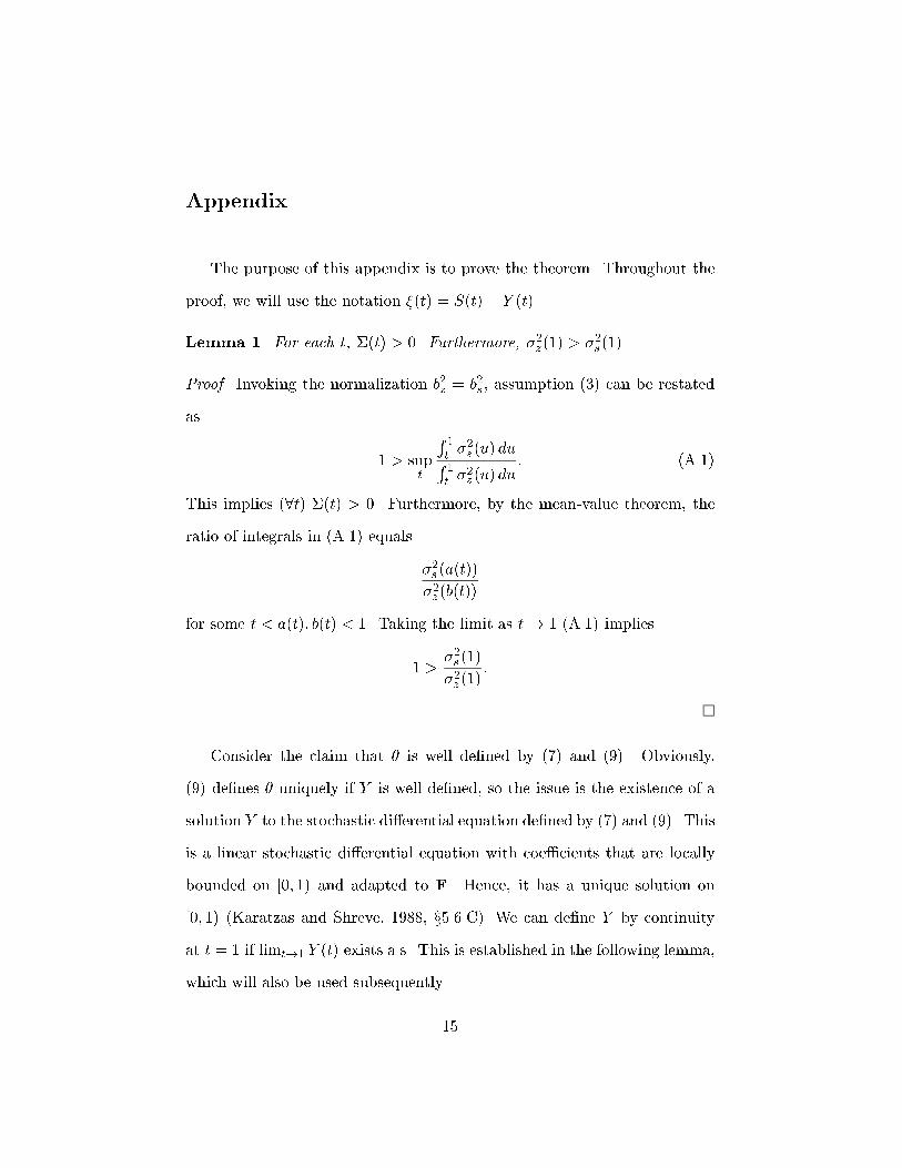
Appendix
The purpose of this appendix is to prove the theorem. Throughout the
proof, we will use the notation �(t) = S(t)� Y (t).
Lemma 1. For each t, �(t) > 0. Furthermore, �2z(1) > �2s(1).
Proof. Invoking the normalization b2z = b2s, assumption (3) can be restated
as
1 > supt
R1
t�2s(u) duR
1
t�2z(u) du
: (A.1)
This implies (8t) �(t) > 0. Furthermore, by the mean-value theorem, the
ratio of integrals in (A.1) equals
�2s(a(t))
�2z(b(t))
for some t < a(t); b(t) < 1. Taking the limit as t! 1 (A.1) implies
1 >�2s(1)
�2z(1):
Consider the claim that � is well de�ned by (7) and (9). Obviously,
(9) de�nes � uniquely if Y is well de�ned, so the issue is the existence of a
solution Y to the stochastic di�erential equation de�ned by (7) and (9). This
is a linear stochastic di�erential equation with coe�cients that are locally
bounded on [0; 1) and adapted to F. Hence, it has a unique solution on
[0; 1) (Karatzas and Shreve, 1988, x5.6.C). We can de�ne Y by continuity
at t = 1 if limt!1 Y (t) exists a.s. This is established in the following lemma,
which will also be used subsequently.
15

Lemma 2. Given the trading strategy (9), limt!1 Y (t) = S(1) a.s.
Proof. The claim is that limt!1 �(t) = 0 a.s. The process � satis�es the
stochastic di�erential equation
d�(t) =��2z(t)
�(t)�(t) dt+ �z(t) dWz(t)� �s(t) dWs(t):
This may be rewritten as
d�(t) =��2z(t)
�(t)�(t) dt+ �(t) dW (t); (A.2)
where �2(t) � �2z(t) + �2s(t); and W is a standard Wiener process.
The solution of the stochastic di�erential equation (A.2) with initial
condition �(0) = S(0) is (Karatzas and Shreve, 1988, x5.6C)
�(t) = ��1(t)
�S(0) +
Z t
0
�(u)�(u) dW (u)
�;
where
�(t) � exp
�Z t
0
�2z(u)��1(u) du
�:
Here, and in the following argument, the inverse notation �1 denotes the
reciprocal. The desired result �(t)! 0 a.s. as t! 1 will follow from showing
��1(t)! 0 (A.3)
and
��1(t)
Z t
0
�(u)�(u) dW (u)! 0a.s. (A.4)
as t! 1. In the proofs of these results, we will use without further comment
the facts that �2z(�) and �2(�) are continuous, strictly positive functions and
hence are bounded above and bounded away from zero. Likewise, �2z(�) �
16

�2s(�) is bounded above, and it is bounded away from zero on a neighborhood
of t = 1 by virtue of continuity and Lemma 1.
To prove (A.3), it su�ces to show thatR t0��1(u) du !1. An applica-
tion of the mean-value theorem gives, for each u and some u� 2 [u; 1],
�(u) = ��0(u�)(1 � u) = [�2z(u�)� �2s(u
�)](1� u) � a(1� u)
for some constant a. Therefore
Z t
0
��1(u) du � a�1Z t
0
(1� u)�1 du!1:
It remains to establish (A.4). It su�ces to show that
��1(t)
Z t
0
�(u) dW (u)! 0a.s.
Applying the law of the iterated logarithm to the continuous local martingaleR t0�(u) dW (u) (Durrett, 1984, p. 77) gives
lim supt!1
R t0�(u)dW (u)q
2R t0�2(u) du � log log
R t0�2(u) du
= 1:
Hence, it su�ces to show that
��1(t)
s2
Z t
0
�2(u) du � log log
Z t
0
�2(u) du! 0;
equivalently,
2R t0�2(u) du � log log
R t0�2(u) du
�2(t)! 0: (A.5)
This follows from (A.3) unless
Z t
0
�2(u) du!1; (A.6)
17

so suppose (A.6) holds.
The proof of (A.5) now follows from repeated application of l'Hopital's
rule. A �rst application, combined with dropping bounded factors and terms
known to converge to zero, shows that it su�ces to establish
log logR t0�2(u) du
1=�(t)! 0:
A second application, again dropping bounded factors, shows that it su�ces
to establish
�2(t)�2(t)R t0�2(u) du � log
R t0�2(u) du
! 0:
A third application shows that it su�ces to establish
�2s(t)�(t)
1 + logR t0�2(u) du
! 0;
and this is clearly true.
We now establish the claim regarding the FY (t)-conditional distribution
of S(t).
Lemma 3. For each t, the FY (t)-conditional distribution of S(t) is normal
with mean Y (t) and variance �(t).
Proof. We have
d�(t) = ��(t)�(t) dt� �z(t) dWz(t) + �s(t) dWs(t);
dY (t) = �(t)�(t) dt + �z(t) dWz(t);
where �(t) = �2z(t)=�(t). These are the state (or signal) and observation
equations, in the terminology of �ltering. Conditional on FY (t), �(t) is
18

normally distributed. We will denote its conditional mean by �(t) and its
conditional variance by ��(t). Therefore, S(t) is conditionally normal with
mean �(t) + Y (t) and variance ��(t).
The Kalman-Bucy �ltering equation for �(t) is8
d�(t) = ��(t)�(t)dt+1
�z(t)[�(t)��(t)� �2z(t)] d�(t); (A.7)
with initial condition �(0) = E[S(0)] = 0. In (A.7), � denotes a Wiener
process (the innovations process). The variance process �� satis�es the
di�erential equation
d
dt��(t) = �2�(t)��(t) + �2z(t) + �2s(t)�
1
�2z(t)[�(t)��(t)� �2z(t)]
2
and initial condition
��(0) = var �(0) = �20 :
This Riccati equation is well known to have a unique solution. It is easy to
check that it is solved by �� = �, which shows that � is the conditional
variance of S(t).
Substituting �� = � into (A.7), it becomes
d�(t) = ��(t)�(t) dt:
The unique solution of this with initial condition �(0) = 0 is � � 0. Hence,
the conditional mean of S(t) is Y (t).
The next two lemmas establish that (P; �) is an equilibrium.
Lemma 4. Given the trading strategy (9), the pricing rule (10) is compet-
itive.
19

Proof. Using successively the facts that Y (1) = S(1) a.s., the fact that S
has independent zero-mean increments, and Lemma 3, we obtain
E[Y (1)jFY (t)] = E[S(1)jFY (t)]
= E[S(t)jFY (t)]
= Y (t):
Hence, Y is a martingale relative to the �ltration FY . L�evy's theorem
(Karatzas and Shreve, 1988, p. 157) therefore implies that the processes
(Y;FY ) and (Z;FZ) are equivalent in law. Successively applying the law of
iterated expectations, the fact that Y (1) = S(1) a.s., and this equivalence
in law gives
E[~vjFY (t)] = E[f(S(1))jFY (t)]
= E[f(Y (1))jFY (t)]
=
Z1
�1
f(y)�(t; Y (t); y) dy;
which completes the proof.
Lemma 5. Given the pricing rule (10), the trading strategy (9) is optimal.
Proof. Let � denote a generic trading strategy for the informed trader. The
proof depends on establishing a sharp upper bound on the expected wealth
of the informed trader. De�ne
j(s; y) =
Z s
y
(f(s)� f(x)) dx:
20

Let �(t; s; �) denote the density function for the normal distribution with
mean s and varianceR1
t�2s(u) du. For t < 1, de�ne
J(t; s; y) =
Z1
�1
Z1
�1
j(s0; y0)�(t; s; s0)�(t; y; y0) ds0 dy0: (A.8)
Set J(1; s; y) = j(s; y). The function J is continuous at t = 1 (Karatzas and
Shreve, 1988, p. 255).
In the following, we omit writing the arguments of the various functions
and use subscripts on J to denote partial derivatives. Obviously,
(8 y) J(1; s; y) > J(1; s; s) = 0; (A.9)
with equality holding if and only if y = s. Also, one can di�erentiate (A.8)
to obtain9
Jt +1
2�2sJss +
1
2�2zJyy = 0: (A.10)
Applying Ito's Lemma and making use of equation (A.10) we �nd that
J(1; S(1); Y (1)) � J(0; S(0); 0) =Z1
0
Js�s dWs +
Z1
0
Jy� dt+
Z1
0
Jy�z dWz:
Upon applying the expectation operator, the two stochastic integrals
against the Wiener processes vanish,10 and this equation becomes
E
��
Z1
0
Jy� dtjF(0)
�= J(0; S(0); 0) �E [J(1; S(1); Y (1))jF(0)] :
A direct calculation shows that
�Jy = E[~vjF(t)] � P:
21

By iterated expectations, we can write the informed trader's optimization
problem as
max�
E
�Z1
0
fE[~vjF(u)] � P (u; Y (u))g�(u) du
�: (A.11)
Therefore, the objective function takes the value
J(0; S(0); 0) �E[J(1; S(1); Y (1))jF(0)] � J(0; S(0); 0);
with, from (A.9), equality obtaining if and only if S(1) = Y (1) a.s. Since, by
Lemma 2, this equality holds for the strategy (9), that strategy is optimal.
Equation (11) follows from Ito's Lemma, noting that the dt terms cancel
(the explanation is the same as in footnote 9). We can write P (t; y) as
Z1
�1
f(y + u)�(t; 0; u) du:
The assumptions regarding the derivative of f guarantee that we can di�er-
entiate this with respect to y under the integral operator. This gives
�(t; y) =
Z1
�1
f 0(y + u)�(t; 0; u) du:
It follows that �(t; Z(t)) = E[f 0(Z(1))jFZ(t)]. Given the equality of the laws
of (Z;FZ) and (Y;FY ) (see the proof of Lemma 4), this implies �(t; Y (t)) is
the martingale E[f 0(Y (1))jFY (t)].
22

References
Admati, A., and P. P eiderer, 1988, A theory of intraday patterns: Volume
and price variability, Review of Financial Studies 1, 3-40.
Back, K., 1992, Insider trading in continuous time, Review of Financial
Studies 5, 387-409.
Brock, W., and A. Kleidon, 1992, Periodic market closure and trading vol-
ume: A model of intraday bids and asks, Journal of Economic Dynamics
and Control 16, 451-489.
Durrett, R., 1984, Brownian Motion and Martingales in Analysis (Wads-
worth, Belmont, California).
Ferguson, M., Mann, S., and L. Schneck, 1993, Concentrated trading in
the foreign exchange futures markets: Discretionary liquidity trading or
market closure (Division of Economic Analysis, Commodity Futures Trading
Commission, Washington, D.C.).
Foster, F. D., and S. Viswanathan, 1993, Variations in trading volume, re-
turn volatility, and trading costs: Evidence on recent price formation models,
Journal of Finance 48, 187-211.
Grossman, S. J., 1981, An introduction to the theory of rational expectations
under asymmetric information, Review of Economic Studies 48, 541-559.
Harrison, J. M., and D. M. Kreps, 1979, Martingales and arbitrage in mul-
tiperiod securities markets, Journal of Economic Theory 20, 381-408.
Jain, P. C., and G.-H. Joh, 1988, The dependence between hourly prices and
trading volume, Journal of Financial and Quantitative Analysis 23, 269-283.
Kallianpur, G., 1980, Stochastic Filtering Theory (Springer-Verlag, New
York).
Karatzas, I., and S. E. Shreve, 1988, Brownian Motion and Stochastic Cal-
culus (Springer-Verlag, New York).
Kyle, A. S., 1985, Continuous auctions and insider trading, Econometrica
53, 1315-1335.
23

McInish, T. H., and R. A. Wood, 1992, An analysis of intraday patterns in
bid/ask spreads for NYSE stocks, Journal of Finance 47, 753-764.
Madhavan, A., Richardson, M., and M. Roomans, 1994, Why do security
prices change? A transaction-level analysis of NYSE stocks (working paper).
Wood, R. A., McInish, T. H., and J. K. Ord, 1985, An investigation of
transactions data for NYSE stocks, Journal of Finance 723-741.
24
Notes
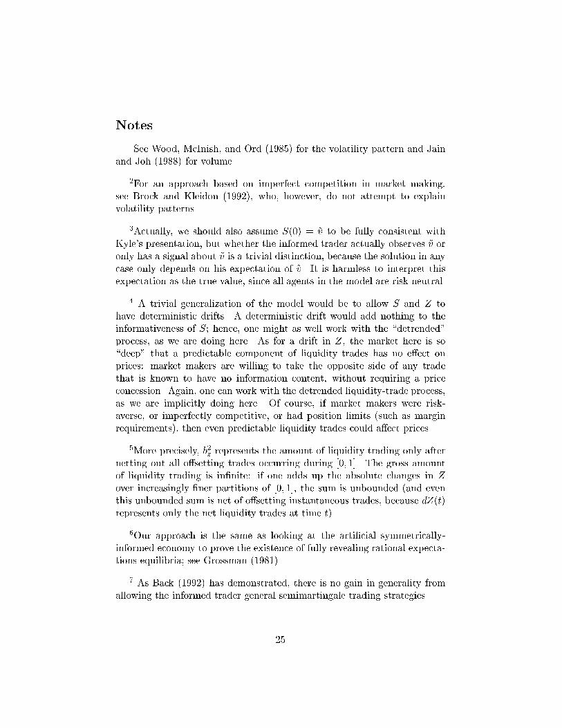
1See Wood, McInish, and Ord (1985) for the volatility pattern and Jain
and Joh (1988) for volume.
2For an approach based on imperfect competition in market making,
see Brock and Kleidon (1992), who, however, do not attempt to explain
volatility patterns.
3Actually, we should also assume S(0) = ~v to be fully consistent with
Kyle's presentation, but whether the informed trader actually observes ~v or
only has a signal about ~v is a trivial distinction, because the solution in any
case only depends on his expectation of ~v. It is harmless to interpret this
expectation as the true value, since all agents in the model are risk neutral.
4 A trivial generalization of the model would be to allow S and Z to
have deterministic drifts. A deterministic drift would add nothing to the
informativeness of S; hence, one might as well work with the \detrended"
process, as we are doing here. As for a drift in Z, the market here is so
\deep" that a predictable component of liquidity trades has no e�ect on
prices: market makers are willing to take the opposite side of any trade
that is known to have no information content, without requiring a price
concession. Again, one can work with the detrended liquidity-trade process,
as we are implicitly doing here. Of course, if market makers were risk-
averse, or imperfectly competitive, or had position limits (such as margin
requirements), then even predictable liquidity trades could a�ect prices.
5More precisely, b2z represents the amount of liquidity trading only after
netting out all o�setting trades occurring during [0; 1]. The gross amount
of liquidity trading is in�nite: if one adds up the absolute changes in Z
over increasingly �ner partitions of [0; 1], the sum is unbounded (and even
this unbounded sum is net of o�setting instantaneous trades, because dZ(t)
represents only the net liquidity trades at time t).
6Our approach is the same as looking at the arti�cial symmetrically-
informed economy to prove the existence of fully revealing rational expecta-
tions equilibria; see Grossman (1981).
7 As Back (1992) has demonstrated, there is no gain in generality from
allowing the informed trader general semimartingale trading strategies.
25

8 See Kallianpur (1980, x10.2). The state and observation equations are
written in Kallianpur's notation as A0(t) = 0; A1(t) = ��(t); A2(t) = 0;
C0(t) = 0; C1(t) = �(t); C2(t) = 0; B(t) = [��z(t); �s(t)]; and D(t) =
[�z(t); 0]:
9See Karatzas and Shreve (1988, p. 254). Note that their regularity
condition (4.3.3), which justi�es di�erentiating (A.8) through the integral
operator, follows from Ef(Z(1))2 = Ef(S(1))2 = E~v2 <1 and the bound
j(s; y) � (s� y)(f(s)� f(y)).
10As explained in footnote 9, we can calculate Jy and Js by di�erentiating
through the integral operator in (A.8). The conditions ER1
0J2y dt <1 and
ER1
0J2s dt <1 follow from the bound on j in footnote 9 and the constraint
(5), and these conditions imply that the stochastic integrals are martingales.
26