Nonlinear Dynhttps://doi.org/10.1007/s11071-021-06297-3

ORIGINAL PAPER

Leveraging circuit theory and nonlinear dynamics for theefficiency improvement of energy harvesting

Michele Bonnin · Fabio L. Traversa · Fabrizio Bonani

Received: 17 September 2020 / Accepted: 6 February 2021© The Author(s) 2021

Abstract We study the performance of vibrationalenergy harvesting systems with piezoelectric and mag-netic inductive transducers, assuming the power ofexternal disturbance concentrated around a specific fre-quency. Both linear and nonlinear harvester models areconsidered. We use circuit theory and equivalent cir-cuits to show that a large improvement in both the har-vested energy and the power efficiency is obtained, forlinear systems, through a proper reactive modificationof the load. For nonlinear systems, we use methods ofnonlinear dynamics to derive analytical formulae forthe output voltage, the harvested energy and the powerefficiency.We show that also for the nonlinear case, themodified load significantly boosts the performance.

Keywords Energy harvesting · Nonlinear oscillators ·Equivalent circuits ·Loadmatching · Power efficiency ·Nonlinear resonance

M. Bonnin (B) · F. BonaniDipartimento di Elettronica e Telecomunicazioni,Politecnico di Torino, Turin, Italye-mail: michele.bonnin@polito.it

F. Bonanie-mail: fabrizio.bonani@polito.it

F. L. TraversaMemComputing Inc., San Diego, CA, USAe-mail: ftraversa@memcpu.com

1 Introduction

Bolstered by the rapid deployment of the Industry 4.0paradigm, the proliferation of Internet of Things (IoT)applications is expected to reach 31 billion connecteddevices by 2020, and 75 billion devices by 2025 [1].At the very foundation of IoT lies the idea that a net-work of devices with embedded electronics, sensors,actuators and software are connected and interact viathe Internet [2–4]. Among the many challenges posedby IoT, the problem of how to supply power to thisnetwork of wireless nodes is of paramount importance.Although the power needed to operate each device issmall, typically in the microwatt to milliwatt range,their huge number, their often remote and difficult toaccess location and their ongoingminiaturizationmakeold fashioned solutions, e.g., batteries, quite rarely aviable approach. A striking example are wearable sys-tems, which are both portable and wireless, and thuswhere batteries would be an obvious choice. Unfortu-nately, the progress in energy storage density has, forthe moment, been unable to keep the pace and batteriesremain, with respect to other electronic components,bulky and heavy [5,6].

A significant literature body, see, e.g., [7–9], sug-gests that electronic systems capable to wirelesslyexchange not only information but also energy mayrepresent a valid alternative. Yet another solution isto design systems capable of self-powering, by scav-enging energy from the surrounding environment. Thecollected power can be used as a direct power source,

123

M. Bonnin et al.

or at least to extend the battery lifespan for those sys-tems where continuous operation without maintenanceis required. The set of technical solutions exploitingthis idea is referred to as energy harvesting [10–12].

Energy harvesting (EH) technologies exploit differ-ent physical principles, depending upon the externalpower source to be tapped. Irrespective of the work-ing principle, a common issue of EH apparatuses is thelimited power density of the source. However, althoughnegligible at the macroscale, energy dispersed in theenvironment is significant at the microscale, makingEH technologies a viable solution to powering smallautonomous devices.

Among the many possible sources, kinetic energyplays a very prominent role, because of its compar-atively large power density and its widespread avail-ability. Kinetic energy exists in the form of mechanicalvibrations, regular or random displacements and driv-ing forces. It can be found in mechanical structures,due to impacts or periodic motions, in buildings andbridges, due to traffic and wind, in vehicles, due toroad asperity and engine induced vibrations, as well asin human body motion [13–16].

Kinetic energy harvesters rely on some kind of oscil-lating structure to capture vibrations, and on a trans-ducer that converts kinetic energy into electrical power.Linear energy harvesters require a fine tuning of theoscillator’s resonant frequency, to match the spectralrange of environmental vibrations where most of theenergy is concentrated. In many applications, this isa key limiting factor, due to geometrical and dimen-sional constraints. In fact, the rule of thumb is thatthe smaller is the size of an object, the larger its res-onant frequency will be. Thus, it is very difficult todesign energy harvesters that are both miniaturized andthat work efficiently at low frequencies, making, forinstance, the realization of wearable electronics thatscavenge energy from human body motion very chal-lenging. In this respect, it has been suggested that non-linear oscillators can perform better than linear ones[17–22]. When compared to their linear counterparts,nonlinear energy harvesters show a wider steady-statefrequency bandwidth and may exhibit multi-stabilityand even chaotic dynamics, thus suggesting that theycan be more efficient especially in random and non-stationary vibratory environments [23–26].

Oscillators periodically exchange energy betweentwodifferent forms.The losses takingplace during eachoscillation cycle, both dissipated by internal resistances

and delivered to the load, can be significantly less thanthe total energy involved in the oscillation. For exam-ple, an LC oscillator characterized by a quality factorQ loses approximately a fraction 1/Q of its energy peroscillation cycle. The remaining power bounces backand forth between the source and the load. It is wellknown fromcircuit theory that, in order tomaximize thepower efficiency, it is necessary to minimize the powerthat merely flows in the circuit with no useful contri-bution, a procedure known as power factor correction.

In this paper, we apply circuit theory and nonlin-ear dynamics methods to improve the efficiency of EHsystems. We study the equivalent circuits (ECs) fortwo well-known energy harvesters: piezoelectric andmagnetic inductive. Using circuit theory, we show thatfor linear harvesters, a simple modification of the loadinspired by previous works [27–31] allows to improvethemaximumcollected power and the power efficiency.In the nonlinear case, using nonlinear dynamics meth-ods we solve the state equations and find analyticalformulae for the harvested power and the power effi-ciency.We show that, similarly to the linear case, prop-erly modifying the load increases both the harvestedpower and the power efficiency.

The paper is organized as follows. In Sect. 2,we present the harvester models and ECs for bothpiezoelectric- and magnetic induction-based devices,showing how nonlinearities in the mechanical part(stiffness of the rod and in the springs, respectively)can be accounted for in the circuit equations. In Sect. 3,we investigate the linear limit. We apply standard cir-cuit theory to solve the governing equations, and weshow how the harvested energy and power efficiencycan bemaximized by a proper adaptation of the load. InSect. 4, we study the nonlinear case. We show that thegoverning equations can be put in a standard form, validfor both the piezoelectric- and themagnetic inductance-based harvesters.We use tools of nonlinear dynamics tosolve the state equations, and we derive analytical for-mulae for the harvested power and power efficiency.Weshow that even for the nonlinear harvester, the adaptedload outperforms a purely resistive load. Finally, Sect. 5is devoted to conclusions.

2 Harvester modeling

An EH device for mechanical vibration scavenging iscomposed by an oscillator that captures kinetic energy

123

Leveraging circuit theory and nonlinear dynamics

Piezoelectriclayers

Inertialmass

Motion

xm

support

V ibrating

support

V ibrating

Load

Staticload

Fig. 1 Schematic representation of a piezoelectric energy har-vester

from environmental vibrations, and by a transducer,responsible for the conversion of kinetic energy intousable electrical power. Transducers may exploit dif-ferent physical principles for energy conversion includ-ing piezoelectric, magnetic induction and electrostatictransduction methods.

2.1 Piezoelectric energy harvester

A schematic representation of a piezoelectric energyharvester is shown in Fig. 1.

A simple piezoelectric energy harvester is composedby a cantilever beam, covered by a layer of piezoelec-tric material, fixed at one end to a moving support withan inertial mass m at the opposite end to increase theoscillation amplitude. Vibrations of the support pro-duce oscillations of the cantilever, inducing mechani-cal stress and strain in the piezoelectric material thatare converted into electrical currents.

A more sophisticated setup is shown in Fig. 1[23,32]. A thin beam covered by piezoelectric layersand with an inertial massm is clamped at both ends. Anexternal static load can be applied to one end, to tunethe natural frequency of the beam and to introduce acubic nonlinearity. Under the influence of an externaldynamic excitation, the beam undergoes oscillationsaround a static position defined by the axial load. Ifthe mass of the cantilever and the effect of gravity areneglected, the equation of motion for the mechanicalsystem reads [18,33]

m x = −U ′(x) − γ x − kv v(t) + Fin (1)

where x is the displacement from the vertical equilib-rium position, U (x) is the elastic potential of the can-

+−

+−

R1 C1L1

vin(t)kv v2

+ v1 −

kc i1

C2 +

−v2

i1Load

Mechanical system Electrical domain

i2a

Fig. 2 EC for the piezoelectric harvester

tilever beam and the prime denotes the first derivative,γ is the friction coefficient, kv v(t) describes the actionof the piezoelectric layer onto the mechanical system(v(t) is the transducer voltage), and Fin is the externalperturbation.

The energy of ambient vibrations is typically spreadover a wide frequency range, suggesting to model per-turbation as white Gaussian noise. However, such ran-dom process can be represented as a superposition ofharmonic (sinusoidal) signals with random phases andfrequencies [34]. For the sake of simplicity, we con-sider here a vibration energy concentrated around asingle frequency, and thus, we model vibrations as asimple harmonic driving force.

The piezoelectric device is characterized by an inter-nal capacitanceC2, an internal resistance, here assumedto be negligible for the sake of simplicity, and a cou-pling with the mechanical part represented by param-eter kc.

The EC for the electromechanical system is shownin Fig. 2, where the parallel branches on the right rep-resent the piezoelectric device, feeding a generic load.

Applying Kirchhoff voltage law (KVL) to the leftloop yields

q1 = − 1

L1v1(q1) − R1

L1q1 − kv

L1v2 + 1

L1vin (2)

where q1 = i1(t), and v1(q1) is the voltage–chargecharacteristic of the capacitor C1. It is straightfor-ward to verify that (1) and (2) are equivalent providedx = q1, m = L1, U ′(x) = v1(q1), γ = R1, Fin = vinand v = v2.

Application of Kirchhoff current law (KCL) to nodea on the right yields

v2 = kcC2

q1 − 1

C2i2 (3)

Usually, purely resistive loads are considered [18,33]. However, we will show that both the harvestedpower and the harvester efficiency can be significantlyboosted if the load has a reactive component.

123

M. Bonnin et al.

N S

Coil

Spring Spring

Magnet

Motion

Load

V ibrating

supportsupport

V ibrating

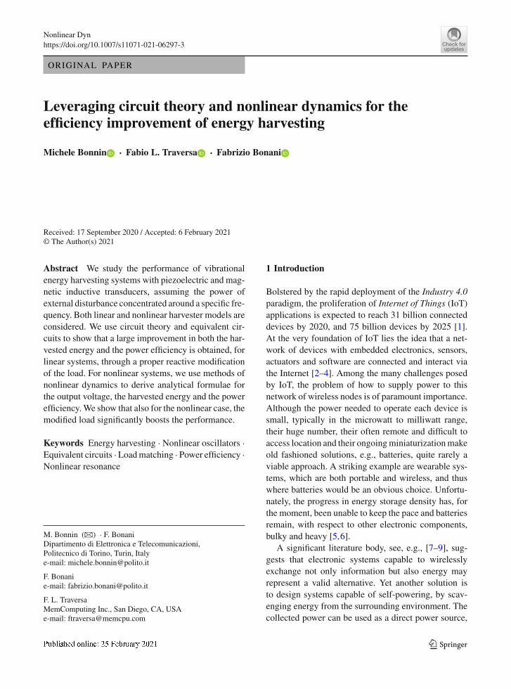
Fig. 3 Schematic representation of an electromagnetic energyharvester

+−

+−

R1 C1L1

vin(t)r1 i2

+ v1 −

r2 i1

+

−v2

i1

Load

Mechanical system Electrical domain

i2

+−

L2

Fig. 4 EC for the electromagnetic harvester

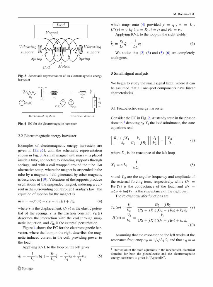
2.2 Electromagnetic energy harvester

Examples of electromagnetic energy harvesters aregiven in [35,36], with the schematic representationshown in Fig. 3. A small magnet with massm is placedinside a tube, connected to vibrating supports throughsprings, and with a coil wrapped around the tube. Analternative setup, where the magnet is suspended in thetube by a magnetic field generated by other magnets,is described in [19]. Vibrations of the supports produceoscillations of the suspended magnet, inducing a cur-rent in the surrounding coil through Faraday’s law. Theequation of motion for the magnet is

m y = −U ′(y) − c y − r1 i(t) + Fin (4)

where y is the displacement, U (y) is the elastic poten-tial of the springs, c is the friction constant, r1i(t)describes the interaction with the coil through mag-netic induction, and Fin is the external perturbation.

Figure 4 shows the EC for the electromagnetic har-vester, where the loop on the right describes the mag-netic induced current in the coil, providing power tothe load.

Applying KVL to the loop on the left gives

q1 = − 1

L1v1(q1) − R1

L1q1 − r1

L1i2 + 1

L1vin (5)

which maps onto (4) provided y = q1, m = L1,U ′(y) = v1(q1), c = R1, i = i2 and Fin = vin

Applying KVL to the loop on the right yields

i2 = r2L2

q1 − 1

L2v2 (6)

We notice that (2)–(3) and (5)–(6) are completelyanalogous.

3 Small signal analysis

We begin to study the small signal limit, where it canbe assumed that all one-port components have linearcharacteristics.

3.1 Piezoelectric energy harvester

Consider the EC in Fig. 2. At steady state in the phasordomain,1 denoting by Y2 the load admittance, the stateequations read

[R1 + j X1 kv

−kc G2 + j B2

] [I1V2

]=

[Vin0

](7)

where X1 is the reactance of the left loop

X1 = ωL1 − 1

ωC1(8)

ω and Vin are the angular frequency and amplitude ofthe external forcing term, respectively, while G2 =Re{Y2} is the conductance of the load, and B2 =ωC2 + Im{Y2} is the susceptance of the right part.

The relevant transfer functions are

Yin(ω) = I1Vin

= G2 + j B2

(R1 + j X1)(G2 + j B2) + kv kc(9)

H(ω) = V2Vin

= kc(R1 + j X1)(G2 + j B2) + kv kc

(10)

Assuming that the resonator on the left works at theresonance frequency ω0 = 1/

√L1C1 and that ω0 = ω

1 Derivation of the state equations in the mechanical–electricaldomains for both the piezoelectric and the electromagneticenergy harvesters is given in “Appendix”.

123

Leveraging circuit theory and nonlinear dynamics

to maximize energy collection, using phasors and (10),the average power delivered to the load is

Pout =1

2Re[V2 I ∗

2 ] = 1

2G2 |V2|2 = 1

2G2 |H |2 |Vin|2

=1

2

G2k2cK 2 + R2

1B22

|Vin|2 (11)

where K = R1G2 + kvkc. Conversely, using (9) theaverage power injected by the voltage source is

Pin =1

2Re[Vin I ∗

1 ] = 1

2Re[Y ∗

in] |Vin|2

=1

2

G2K + R1B22

K 2 + R21B

22

|Vin|2 (12)

so that the power efficiency reads

ηpz = PoutPin

= G2k2cG2K + R1B2

2

(13)

As a result, both the average dissipated power Poutand the power efficiency ηpz are maximized whenthe susceptance B2 is null.2 This condition cannot beattained by a resistive load, as customarily assumed [20,33,35–37]. Conversely, maximum dissipated powerand efficiency are achieved if the load is composedby a resistor R2 = 1/G2 connected in parallel withan inductor L2 with inductance L2 = 1/(ω2

0C2) =L1C1/C2, as shown in Fig. 8 b. In this case, the circuitin Fig. 2 is composed by two resonators with the sameresonant frequency connected through the controlledsources.

A realistic transducer model must represent a pas-sive element, so that it does not supply energy to the restof the circuit. According to the passive sign convention[38], the average power dissipated by the controlledsources is

Pkv + Pkc = 1

2(kv − kc)Re{V2 I ∗

1 }

= 1

2(kv − kc)Re{H(ω) Y ∗

in(ω)}|Vin|2 (14)

2 We do not consider here the case R1 → 0 Ω . For R1 → 0,R2 would be the only resistive load in the circuit, and all activepower supplied by the sourcewould be delivered to the load, with100% efficiency irrespective of the values of parameters L1, C1,C2 and R2.

In particular, at the resonance frequency

Pkv + Pkc = 1

2(kv − kc)

G2 kc(R1 G2 + kvkc)2

|Vin|2 (15)

Equation (15) implies that the transducer is passive ifand only if kv ≥ kc. Considering that dissipation isaccounted for by R1, it can be assumed that the trans-ducer’s energy balance is null for all frequencies, thusimplying kv = kc. For this reason, in many modelsone parameter only is used to describe the transducer[23,31,39].

Maximumaverage dissipated power is obtainedwiththe load conductance

G2 = k2vR1

(16)

corresponding to a maximum average absorbed power

Pmaxout = |Vin|2

8R1(17)

and to the expected 50% efficiency [38].Efficiencyhigher than50%canobviously be attained,

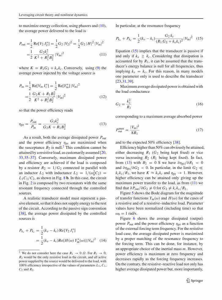
either decreasing R1 (G2 being kept fixed) or viceversa increasing R2 (R1 being kept fixed). In fact,from (13) with B2 = 0 S we have ∂ηpz/∂R1 < 0and ∂ηpz/∂G2 < 0. In particular, in the limit G2 �kckv/R1, we have K ≈ kvkc and ηpz → 1. However,higher efficiency can be attained only giving up themaximum power transfer to the load, as from (11) wefind that ∂Pout/∂G2 = 0 for G2 = kckv/R1.

Figure 5 shows the Bode diagram for the magnitudeof transfer functions Yin(ω) and H(ω) for the cases ofa resistive and of a resistive–inductive load. Parametervalues have been normalized (including time) so thatω0 = 1 rad/s.

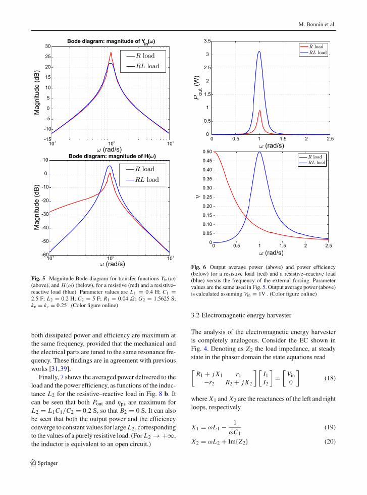
Figure 6 shows the average dissipated (output)power Pout and the power efficiency ηpz as a functionof the external forcing term frequency. For the resistiveload case, the average dissipated power is maximizedby a proper matching of the resonance frequency tothe forcing term. This can be done, for instance, byan appropriate choice of the inertial mass m. However,power efficiency is maximum at zero frequency anddecreases rapidly as the forcing frequency increases.On the contrary, the resistive–reactive load not only hashigher average dissipated power but, more importantly,

123

M. Bonnin et al.

10-1 100 101-15

-10

-5

0

5

10

15

20

25

30Bode diagram: magnitude of Yin( )

(rad/s)

Mag

nitu

de (d

B)

(rad/s)

Mag

nitu

de (d

B)

Bode diagram: magnitude of H( )

10-1 100 101-60

-50

-40

-30

-20

-10

0

10

Fig. 5 Magnitude Bode diagram for transfer functions Yin(ω)

(above), and H(ω) (below), for a resistive (red) and a resistive–reactive load (blue). Parameter values are L1 = 0.4 H; C1 =2.5 F; L2 = 0.2 H; C2 = 5 F; R1 = 0.04 Ω; G2 = 1.5625 S;kv = kc = 0.25 . (Color figure online)

both dissipated power and efficiency are maximum atthe same frequency, provided that the mechanical andthe electrical parts are tuned to the same resonance fre-quency. These findings are in agreement with previousworks [31,39].

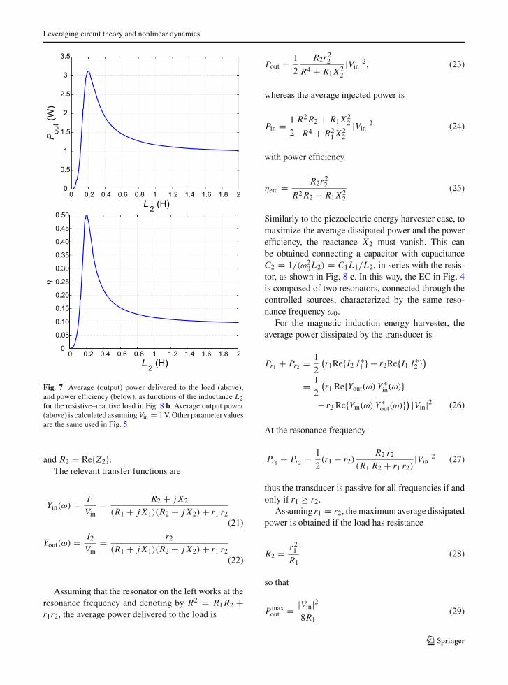
Finally, 7 shows the averaged power delivered to theload and the power efficiency, as functions of the induc-tance L2 for the resistive–reactive load in Fig. 8 b. Itcan be seen that both Pout and ηpz are maximum forL2 = L1C1/C2 = 0.2 S, so that B2 = 0 S. It can alsobe seen that both the output power and the efficiencyconverge to constant values for large L2, correspondingto the values of a purely resistive load. (For L2 → +∞,the inductor is equivalent to an open circuit.)

0 0.5 1 1.5 2 2.50

0.5

1

1.5

2

2.5

3

3.5

(rad/s)

Pou

t(W

)

0

0.05

0.10

0.15

0.20

0.25

0.30

0.35

0.40

0.45

0.50

0 0.5 1 1.5 2 2.5(rad/s)

Fig. 6 Output average power (above) and power efficiency(below) for a resistive load (red) and a resistive–reactive load(blue) versus the frequency of the external forcing. Parametervalues are the same used in Fig. 5. Output average power (above)is calculated assuming Vin = 1V . (Color figure online)

3.2 Electromagnetic energy harvester

The analysis of the electromagnetic energy harvesteris completely analogous. Consider the EC shown inFig. 4. Denoting as Z2 the load impedance, at steadystate in the phasor domain the state equations read

[R1 + j X1 r1

−r2 R2 + j X2

] [I1I2

]=

[Vin0

](18)

where X1 and X2 are the reactances of the left and rightloops, respectively

X1 = ωL1 − 1

ωC1(19)

X2 = ωL2 + Im{Z2} (20)

123

Leveraging circuit theory and nonlinear dynamics

0 0.2 0.4 0.6 0.8 1 1.2 1.4 1.6 1.8 20

0.5

1

1.5

2

2.5

3

3.5

L 2 (H)

Pou

t(W

)

0 0.2 0.4 0.6 0.8 1 1.2 1.4 1.6 1.8 20

0.05

0.10

0.15

0.20

0.25

0.30

0.35

0.40

0.45

0.50

L 2 (H)

Fig. 7 Average (output) power delivered to the load (above),and power efficiency (below), as functions of the inductance L2for the resistive–reactive load in Fig. 8 b. Average output power(above) is calculated assumingVin = 1V.Other parameter valuesare the same used in Fig. 5

and R2 = Re{Z2}.The relevant transfer functions are

Yin(ω) = I1Vin

= R2 + j X2

(R1 + j X1)(R2 + j X2) + r1 r2(21)

Yout(ω) = I2Vin

= r2(R1 + j X1)(R2 + j X2) + r1 r2

(22)

Assuming that the resonator on the left works at theresonance frequency and denoting by R2 = R1R2 +r1r2, the average power delivered to the load is

Pout = 1

2

R2r22R4 + R1X2

2

|Vin|2, (23)

whereas the average injected power is

Pin = 1

2

R2R2 + R1X22

R4 + R21X

22

|Vin|2 (24)

with power efficiency

ηem = R2r22R2R2 + R1X2

2

(25)

Similarly to the piezoelectric energy harvester case, tomaximize the average dissipated power and the powerefficiency, the reactance X2 must vanish. This canbe obtained connecting a capacitor with capacitanceC2 = 1/(ω2

0L2) = C1L1/L2, in series with the resis-tor, as shown in Fig. 8 c. In this way, the EC in Fig. 4is composed of two resonators, connected through thecontrolled sources, characterized by the same reso-nance frequency ω0.

For the magnetic induction energy harvester, theaverage power dissipated by the transducer is

Pr1 + Pr2 = 1

2

(r1Re{I2 I ∗

1 } − r2Re{I1 I ∗2 })

= 1

2

(r1 Re{Yout(ω) Y ∗

in(ω)}− r2 Re{Yin(ω) Y ∗

out(ω)}) |Vin|2 (26)

At the resonance frequency

Pr1 + Pr2 = 1

2(r1 − r2)

R2 r2(R1 R2 + r1 r2)

|Vin|2 (27)

thus the transducer is passive for all frequencies if andonly if r1 ≥ r2.

Assuming r1 = r2, themaximum average dissipatedpower is obtained if the load has resistance

R2 = r21R1

(28)

so that

Pmaxout = |Vin|2

8R1(29)

123

M. Bonnin et al.

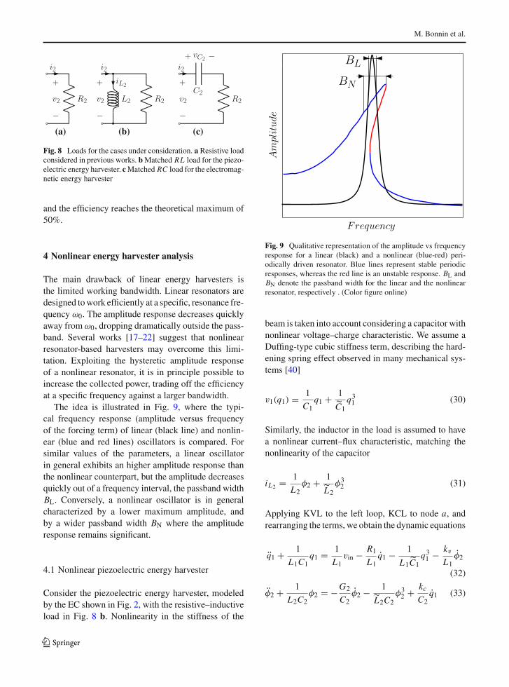
(a) (b) (c)

Fig. 8 Loads for the cases under consideration. a Resistive loadconsidered in previous works. bMatched RL load for the piezo-electric energy harvester. cMatched RC load for the electromag-netic energy harvester

and the efficiency reaches the theoretical maximum of50%.

4 Nonlinear energy harvester analysis

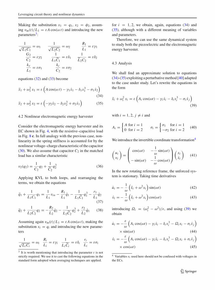
The main drawback of linear energy harvesters isthe limited working bandwidth. Linear resonators aredesigned towork efficiently at a specific, resonance fre-quency ω0. The amplitude response decreases quicklyaway from ω0, dropping dramatically outside the pass-band. Several works [17–22] suggest that nonlinearresonator-based harvesters may overcome this limi-tation. Exploiting the hysteretic amplitude responseof a nonlinear resonator, it is in principle possible toincrease the collected power, trading off the efficiencyat a specific frequency against a larger bandwidth.

The idea is illustrated in Fig. 9, where the typi-cal frequency response (amplitude versus frequencyof the forcing term) of linear (black line) and nonlin-ear (blue and red lines) oscillators is compared. Forsimilar values of the parameters, a linear oscillatorin general exhibits an higher amplitude response thanthe nonlinear counterpart, but the amplitude decreasesquickly out of a frequency interval, the passband widthBL. Conversely, a nonlinear oscillator is in generalcharacterized by a lower maximum amplitude, andby a wider passband width BN where the amplituderesponse remains significant.

4.1 Nonlinear piezoelectric energy harvester

Consider the piezoelectric energy harvester, modeledby the EC shown in Fig. 2, with the resistive–inductiveload in Fig. 8 b. Nonlinearity in the stiffness of the

Amplitude

F requency

BL

BN

Fig. 9 Qualitative representation of the amplitude vs frequencyresponse for a linear (black) and a nonlinear (blue-red) peri-odically driven resonator. Blue lines represent stable periodicresponses, whereas the red line is an unstable response. BL andBN denote the passband width for the linear and the nonlinearresonator, respectively . (Color figure online)

beam is taken into account considering a capacitor withnonlinear voltage–charge characteristic. We assume aDuffing-type cubic stiffness term, describing the hard-ening spring effect observed in many mechanical sys-tems [40]

v1(q1) = 1

C1q1 + 1

C1q31 (30)

Similarly, the inductor in the load is assumed to havea nonlinear current–flux characteristic, matching thenonlinearity of the capacitor

iL2 = 1

L2φ2 + 1

L2φ32 (31)

Applying KVL to the left loop, KCL to node a, andrearranging the terms, we obtain the dynamic equations

q1 + 1

L1C1q1 = 1

L1vin − R1

L1q1 − 1

L1C1q31 − kv

L1φ2

(32)

φ2 + 1

L2C2φ2 = −G2

C2φ2 − 1

L2C2φ32 + kc

C2q1 (33)

123

Leveraging circuit theory and nonlinear dynamics

Making the substitution x1 = q1, x2 = φ2, assum-ing vin(t)/L1 = εA cos(ω t) and introducing the newparameters3:

1√L1C1

= ω11√L2C2

= ω2R1

L1= εγ1

G2

C2= εγ2

1

L1C1= εδ1

1

L2C2= εδ2

kv

L1= εσ1

kcC2

= εσ2

equations (32) and (33) become

x1 + ω21 x1 = ε

(A cos(ω t) − γ1 x1 − δ1x

31 − σ1 x2

)(34)

x2 + ω22 x2 = ε

(−γ2 x2 − δ2x

32 + σ2 x1

)(35)

4.2 Nonlinear electromagnetic energy harvester

Consider the electromagnetic energy harvester and itsEC shown in Fig. 4, with the resistive–capacitive loadin Fig. 8 c. In full analogy with the previous case, non-linearity in the spring stiffness is accounted for by thenonlinear voltage–charge characteristic of the capacitor(30). We also assume that capacitor C2 in the matchedload has a similar characteristic

v2(q2) = 1

C2q2 + 1

C2q32 (36)

Applying KVL to both loops, and rearranging theterms, we obtain the equations

q1 + 1

L1C1q1 = 1

L1vin − R1

L1q1 − 1

L1C1q31 − r1

L1q2

(37)

q2 + 1

L2C2q2 = − R2

L2q2 − 1

L2C2q32 + r2

L2q1 (38)

Assuming again vin(t)/L1 = εA cos(ω t), making thesubstitution xi = qi and introducing the new parame-ters

1√LiCi

= ωiRi

Li= εγi

1

Li Ci= εδi

riLi

= εσi

3 It is worth mentioning that introducing the parameter ε is notstrictly required. We use it to cast the following equations in thestandard form adopted when averaging techniques are applied.

for i = 1, 2, we obtain, again, equations (34) and(35), although with a different meaning of variablesand parameters.

Therefore, we can use the same dynamical systemto study both the piezoelectric and the electromagneticenergy harvester.

4.3 Analysis

We shall find an approximate solution to equations(34)-(35) exploiting a perturbativemethod [40] adaptedto the case under study. Let’s rewrite the equations inthe form

xi + ω2i xi = ε

(Ai cos(ωt) − γi xi − δi x

3i − σi x j

)(39)

with i = 1, 2, j = i and

Ai ={A for i = 10 for i = 2

σi ={

σ1 for i = 1−σ2 for i = 2

(40)

We introduce the invertible coordinate transformation4

(uivi

)=

⎛⎜⎝

cos(ωt) − 1

ωsin(ωt)

− sin(ωt) − 1

ωcos(ωt)

⎞⎟⎠

(xixi

)(41)

In the new rotating reference frame, the unforced sys-tem is stationary. Taking time derivatives

ui = − 1

ω

(xi + ω2xi

)sin(ωt) (42)

vi = − 1

ω

(xi + ω2xi

)cos(ωt) (43)

introducing Ωi = (ω2i − ω2)/ε, and using (39) we

obtain

ui = − ε

ω

(Ai cos(ωt) − γi xi − δi x

3i − Ωi xi − σi x j

)

× sin(ωt) (44)

vi = − ε

ω

(Ai cos(ωt) − γi xi − δi x

3i − Ωi xi + σi x j

)

× cos(ωt) (45)

4 Variables vi used here should not be confused with voltages inthe ECs.

123

M. Bonnin et al.

Inverting (41) and substituting into (44)–(45), weobtain a system of non-autonomous ordinary differen-tial equations in the unknowns ui and vi .

For small value of ε, Eqs. (44) and (45) can be aver-aged introducing a limited error. Integrating each func-tionwith respect to t from0 toT = 2π/ωwhile holdingui and vi constant, we obtain the autonomous system5

ui = − ε

2ω

(γi ω ui + 3

4δi (u

2i + v2i )vi + Ωivi + σi ω u j

)

(46)

vi = − ε

2ω

(Ai + γi ω vi − 3

4δi (u

2i + v2i )ui − Ωi ui

+σi ω v j)

(47)

Introducing polar coordinates

ui = ai cosϕi vi = ai sin ϕi , (48)

a straightforward calculation gives

ai = − ε

2ω

(Ai sin ϕi + γi ω ai + σi ω a j cos(ϕi − ϕ j )

)(49)

ϕi = − ε

2ω

(Ωi − Ai

aicosϕi + 3

4δi a

2i

+ σiωa j

aisin(ϕi − ϕ j )

)(50)

The equilibrium points of equations (49) and (50)correspond to oscillations of constant amplitude in theoriginal equations. They are found solving the system(ψ = ϕ2 − ϕ1)

A sin ϕ1 + γ1ω a1 + σ1ω a2 cosψ = 0 (51)

γ2ω a2 − σ2ω a1 cosψ = 0 (52)

− A cosϕ1 + 3

4δ1 a

31 + Ω1a1 − σ1ω a2 sinψ = 0

(53)

3

4δ2 a

32 + Ω2a2 − σ2ω a1 sinψ = 0 (54)

Equations (52) and (54) imply

cosψ = γ2

σ2

a2a1

(55)

5 With some abuse of notation, we use the same symbols ui andvi to denote also the averaged quantities.

sinψ =34δ2a

32 + Ω2 a2σ2ωa1

(56)

Squaring and summing, we obtain the first equation forthe steady-state amplitudes

γ 22 ω2a22 +

(3

4δ2a

32 + Ω2a2

)2

− σ 22 ω2a21 = 0 (57)

Substituting (55) and (56) into (51) and (53), respec-tively, rearranging the terms, squaring and summing,we find the second amplitude equation

− A2a21 +(

γ1ωa21 + γ2ω

σ1

σ2a22

)2

+

+(3

4δ1a

41 + Ω1a

21 − σ1

σ2a2

(3

4δ2a

32 + Ω2a2

))2

= 0

(58)

The nonlinear algebraic system (57)–(58) can be solvednumerically, finding the steady-state amplitudes a1 anda2. These, in turn, allow to compute the phase shifts ϕ1

andϕ2 through (55)–(56), and finally the state variables

i1(t) = x1(t) = −ωa1 sin(ωt + ϕ1) (59)

v2(t)i2(t)

}= x2(t) = −ωa2 sin(ωt + ϕ2)

{for pzfor em

(60)

The average injected power for both the piezoelec-tric and the electromagnetic energy harvester is

Pin = 1

T

∫ T

0vin(t) q1(t)dt

= − εA L1ωa1T

∫ T

0sin(ωt + ϕ1) cos(ωt)dt

= − εAL1ω a12

sin ϕ1 = εL1ω2

2σ2

(γ1σ2a

21 + γ2σ1a

22

)(61)

where the inverse of (41) has been used, together with(51) and (55).

The average dissipated power for the piezoelectricharvester is

Ppzout = 1

T

∫ T

0

v2(t)2

R2dt

= ω2a22T R2

∫ T

0sin2(ωt + ϕ2)dt = ω2a22

2R2(62)

123

Leveraging circuit theory and nonlinear dynamics

0.2 0.4 0.6 0.8 1 1.2 1.4 1.6 1.8 20

5

10

15

20

25A

mpl

itude

(A)

0(rad/s)

Fig. 10 Input current amplitude for the nonlinear coupled res-onators. Lines derive from the theoretical analysis, while sym-bols result from numerical simulations: Blue circles refer to theresistive–inductive load. Parameters are δ1 = 0.1, δ2 = 0.5,Vin = 1 V, and other parameters are the same as in Fig. 5 . (Colorfigure online)

with power efficiency

ηpz = σ2 G2 a22εL1

(γ1σ2a21 + γ2σ1a22

) (63)

For the electromagnetic energy harvester, the aver-age dissipated power is

Pemout = 1

T

∫ T

0R2 q2(t)

2dt = ω2R2a222

(64)

with power efficiency

ηem = σ2 R2 a22εL1

(γ1σ2a21 + γ2σ1a22

) (65)

To confirm our theoretical prediction, we have per-formed extensive numerical simulations. The followingresults refer to the case of the piezoelectric EH model.Based on the analogy shown at the beginning of thissection, the results can be easily adapted to the case ofelectromagnetic energy harvester.

Figures 10 and 11 show the amplitude response forthe current i1(t) and the voltage v2(t), respectively, asa function of the voltage source angular frequency ω,for the piezoelectric nonlinear energy harvester.

As expected, both curves show the hysteretic behav-ior due to the nonlinear stiffness. Stability and bifurca-

0 0.2 0.4 0.6 0.8 1 1.2 1.4 1.6 1.8 20

1

1.2

1.4

(rad/s)

Am

plitu

de (V

)

0.2

0.4

0.6

0.8

Fig. 11 Output voltage amplitude comparison for a nonlin-ear resonator-based energy harvester: Resistive load versusresistive–inductive load. Black diamonds refer to the resistiveload. Parameters are the same as in Fig. 10

tion analysis for the averaged system are determinedcomputing the eigenvalues of the Jacobian matrix ofsystem (49)–(50). For small values of the forcing fre-quency, there is only one solution, which is a stableequilibrium point of the averaged system and corre-sponds to stable periodic oscillations of i1(t) and v2(t)(increasing full black line), with the same period ofthe forcing term. At the critical value ωSN1 � 1.31,a saddle node bifurcation, identified by a null eigen-value, occurs. Two new, initially coincident, equilib-rium points emerge that separate and become distinctwhenω is further increased. The smaller amplitude cor-responds to a stable equilibrium point (decreasing fullline), while the larger amplitude is a saddle (dashedline). At the critical value ωSN2 � 1.57 rad/s, theunstable saddle collides with the larger, stable equi-librium point, and they vanish through a second sad-dle node bifurcation. The small, stable equilibriumpoint ultimately survives as the only solution. The-oretical predictions of our perturbation approach arecompared with the results obtained from the numericalintegration of equations (32)-(33) (symbols). Numer-ical solutions were obtained applying a continuationmethod, using the solution for a certain value of theforcing frequency as the initial condition for the follow-ing value of this parameter. Obviously, the saddle-typelimit cycle cannot be detected neither through forwardnor backward time integration.Moreover, as the param-eter ω approaches the critical value ωSN2 , it becomes

123

M. Bonnin et al.

increasingly difficult to follow the large stable solu-tion, because its basin of attraction becomes smaller(this solution and the unstable saddle-type limit cycleget closer to each other), and trajectories are attractedtoward the small stable limit cycle.

For comparison purposes, Fig. 11 also shows theoutput voltage for the resistive load case. This valuehas been calculated solving numerically the ODE sys-tem (2)-(3) for the resistive load. The output voltagecurve shows a clear resemblance to the linear case,though with a high, long right tale. This behavior is dueto the resonance between the output voltage v2(t) andthe nonlinear hysteretic behavior of the current i1(t).The maximum amplitude is also shifted toward higherfrequency values. More importantly, the matched RLload case clearly outperforms the resistive load case ina wide frequency interval.

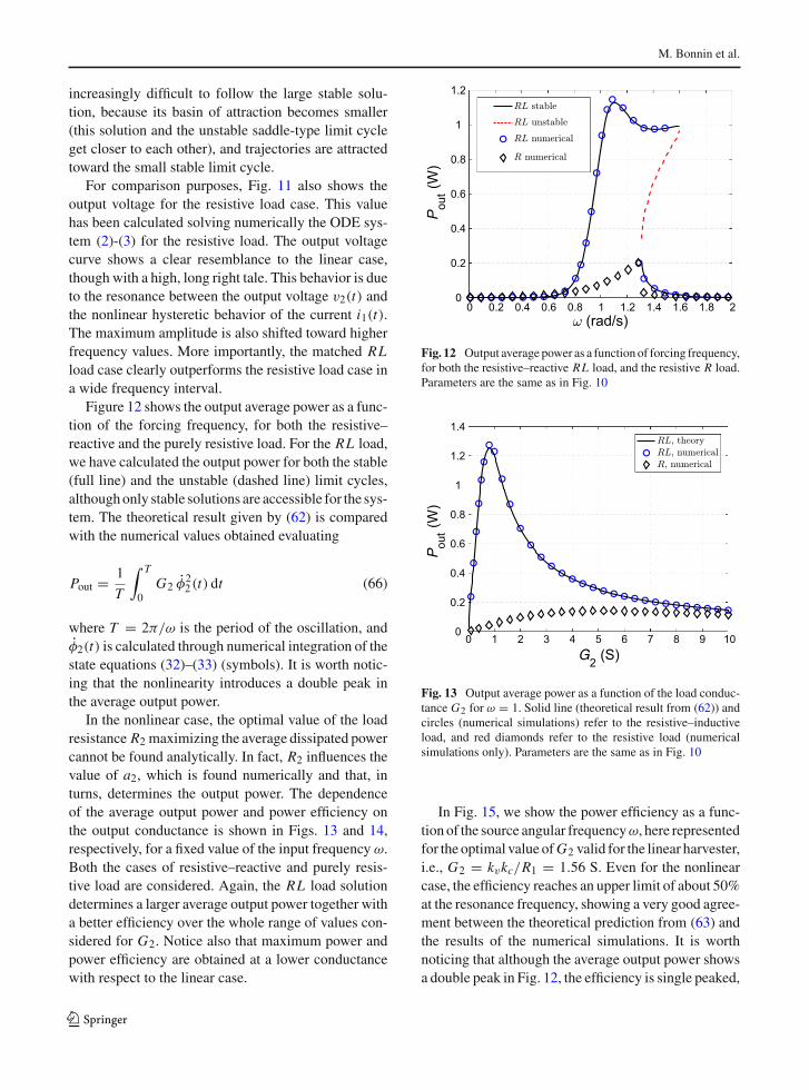
Figure 12 shows the output average power as a func-tion of the forcing frequency, for both the resistive–reactive and the purely resistive load. For the RL load,we have calculated the output power for both the stable(full line) and the unstable (dashed line) limit cycles,althoughonly stable solutions are accessible for the sys-tem. The theoretical result given by (62) is comparedwith the numerical values obtained evaluating

Pout = 1

T

∫ T

0G2 φ2

2(t) dt (66)

where T = 2π/ω is the period of the oscillation, andφ2(t) is calculated through numerical integration of thestate equations (32)–(33) (symbols). It is worth notic-ing that the nonlinearity introduces a double peak inthe average output power.

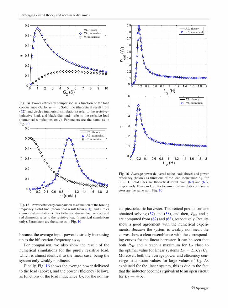
In the nonlinear case, the optimal value of the loadresistance R2 maximizing the average dissipated powercannot be found analytically. In fact, R2 influences thevalue of a2, which is found numerically and that, inturns, determines the output power. The dependenceof the average output power and power efficiency onthe output conductance is shown in Figs. 13 and 14,respectively, for a fixed value of the input frequency ω.Both the cases of resistive–reactive and purely resis-tive load are considered. Again, the RL load solutiondetermines a larger average output power together witha better efficiency over the whole range of values con-sidered for G2. Notice also that maximum power andpower efficiency are obtained at a lower conductancewith respect to the linear case.

0 0.2 0.4 0.6 0.8 1 1.2 1.4 1.6 1.8 20

0.2

0.4

0.6

0.8

1

1.2

(rad/s)

Pou

t(W

)

Fig. 12 Output average power as a function of forcing frequency,for both the resistive–reactive RL load, and the resistive R load.Parameters are the same as in Fig. 10

0 1 2 3 4 5 6 7 8 9 100

0.2

0.4

0.6

0.8

1

1.2

1.4

G2 (S)

Pou

t(W

)

Fig. 13 Output average power as a function of the load conduc-tance G2 for ω = 1. Solid line (theoretical result from (62)) andcircles (numerical simulations) refer to the resistive–inductiveload, and red diamonds refer to the resistive load (numericalsimulations only). Parameters are the same as in Fig. 10

In Fig. 15, we show the power efficiency as a func-tion of the source angular frequencyω, here representedfor the optimal value ofG2 valid for the linear harvester,i.e., G2 = kvkc/R1 = 1.56 S. Even for the nonlinearcase, the efficiency reaches an upper limit of about 50%at the resonance frequency, showing a very good agree-ment between the theoretical prediction from (63) andthe results of the numerical simulations. It is worthnoticing that although the average output power showsa double peak in Fig. 12, the efficiency is single peaked,

123

Leveraging circuit theory and nonlinear dynamics

0 1 2 3 4 5 6 7 8 9 100

0.1

0.2

0.3

0.4

0.5

0.6

G2 (S)

Fig. 14 Power efficiency comparison as a function of the loadconductance G2 for ω = 1. Solid line (theoretical result from(62)) and circles (numerical simulations) refer to the resistive–inductive load, and black diamonds refer to the resistive load(numerical simulations only). Parameters are the same as inFig. 10

0 0.2 0.4 0.6 0.8 1 1.2 1.4 1.6 1.8 20

0.1

0.2

0.3

0.4

0.5

0.6

(rad/s)

Fig. 15 Power efficiency comparison as a function of the forcingfrequency. Solid line (theoretical result from (63)) and circles(numerical simulations) refer to the resistive–inductive load, andred diamonds refer to the resistive load (numerical simulationsonly). Parameters are the same as in Fig. 10

because the average input power is strictly increasingup to the bifurcation frequency ωSN2 .

For comparison, we also show the result of thenumerical simulations for the purely resistive load,which is almost identical to the linear case, being thesystem only weakly nonlinear.

Finally, Fig. 16 shows the average power deliveredto the load (above), and the power efficiency (below),as functions of the load inductance L2, for the nonlin-

0 0.2 0.4 0.6 0.8 1 1.2 1.4 1.6 1.8

0.1

0.2

0.3

0.4

0.5

0.6

0.7

0.8

0.9

20

L 2 (H)

Pou

t(W

)

0 0.2 0.4 0.6 0.8 1 1.2 1.4 1.6 1.8 20

0.1

0.2

0.3

0.4

0.5

0.6

L 2 (H)

Fig. 16 Average power delivered to the load (above) and powerefficiency (below) as functions of the load inductance L2, forω = 1. Solid lines are theoretical result from (62) and (63),respectively. Blue circles refer to numerical simulations. Param-eters are the same as in Fig. 10

ear piezoelectric harvester. Theoretical predictions areobtained solving (57) and (58), and then, Pout and η

are computed from (62) and (63), respectively. Resultsshow a good agreement with the numerical experi-ments. Because the system is weakly nonlinear, thecurves show a clear resemblance with the correspond-ing curves for the linear harvester. It can be seen thatboth Pout and η reach a maximum for L2 close tothe optimal value for linear systems L2 = L1C1/C2.Moreover, both the average power and efficiency con-verge to constant values for large values of L2. Asexplained for the linear system, this is due to the factthat the inductor becomes equivalent to an open circuitfor L2 → +∞.

123

M. Bonnin et al.

5 Conclusions

We have analyzed vibrational energy harvesting sys-tems with piezoelectric and magnetic inductive trans-ducers, assuming the power of external disturbanceconcentrated around a specific frequency.

Typically, energy harvesters are modeled as oscil-lators, either linear or nonlinear, coupled to first-ordersystems that describe the transducer’s dynamics. Forlinear harvester, we used circuit theory to show that theharvested energy can be maximized by a proper match-ing of the load, usually assumed to be a simple resistor.Analogously to the power factor correction procedure,a reactive passive component can be added that max-imizes the average power delivered to the load. As aresult, the energy harvester is modeled by two coupledoscillators that must be designed to have the same res-onance frequency. This solution allows for maximumpower collection by the non-degenerate resistive loadin the presence of finite losses of the harvester. More-over, the maximum 50% efficiency under maximumpower transfer condition can be achieved at the sameresonant frequency.

For the nonlinear system, we used nonlinear dynam-ics methods to derive analytical formulae for the out-put, the harvested energy and the power efficiency. Infull analogy with the linear case, modifying the loadincreases the harvested energy and power efficiency.As opposed to the linear case, however, the efficiencycan reach values above 50%, again assuming realisticvalues for both the load and the harvester losses.

Funding Open access funding provided byPolitecnico di Torinowithin the CRUI-CARE Agreement.

Compliance with ethical standard

Conflict of interest The authors declare that they have no con-flict of interest.

Open Access This article is licensed under a Creative Com-mons Attribution 4.0 International License, which permitsuse, sharing, adaptation, distribution and reproduction in anymedium or format, as long as you give appropriate credit to theoriginal author(s) and the source, provide a link to the CreativeCommons licence, and indicate if changes were made. Theimages or other third party material in this article are includedin the article’s Creative Commons licence, unless indicatedotherwise in a credit line to the material. If material is notincluded in the article’s Creative Commons licence and yourintended use is not permitted by statutory regulation or exceedsthe permitted use, you will need to obtain permission directly

from the copyright holder. To view a copy of this licence, visithttp://creativecommons.org/licenses/by/4.0/.

Appendix: State equations for the electrical domain

In this “Appendix,” we derive the state equationsfor both the mechanical and electrical domains ofthe piezoelectric and the electromagnetic energy har-vesters.

For the piezoelectric energy harvester, the stateequations for the electromechanical system are (1), (3)that we rewrite in the form

x = − U ′(x)m

− γ

mx − kv

mv2 + 1

mFin (67a)

v2 = kcC2

x − 1

C2i2 (67b)

For the resistive load in Fig. 8 a, i2 = G2v2, thusobtaining the electromechanical model equations in[18,33]. For the RL load in Fig. 8 b, applying KCLyields i2 = G2v + iL2 . Using the constitutive relationfor the inductor φ2 = L2iL2 , and the flux–voltage rela-tionship φ2 = v, equations (67) become

x = − U ′(x)m

− γ

mx − kv

mφ2 + 1

mFin (68a)

φ2 = kcC2

x − 1

L2C2φ2 − G2

C2φ2 (68b)

For the electromagnetic energy harvester, the elec-tromechanical equations are (4) and (6) that we rewritein the form

y = − U ′(y)m

− c

my − r1

mi2 + Fin

m(69a)

i2 = r2L2

y − v2

L2(69b)

For the resistive load in Fig. 8 a, v2 = R2i2.For the RC load in Fig. 8 c, applying KVL yields

v2 = R2i2 + vC2 . Using the constitutive relation forthe capacitor q2 = C2vC2 , and the current–charge rela-tionship q2 = i2, equation (69) becomes

y = − U ′(y)m

− c

my − r1

mq2 + Fin

m(70a)

q2 = r2L2

y − 1

L2C2q2 − R2

L2q2 (70b)

123

Leveraging circuit theory and nonlinear dynamics

References

1. Internet of things (IoT) connected devices installed baseworldwide from 2015 to 2025. https://www.statista.com/statistics/471264/iot-number-of-connected-devices-worldwide/. Accessed: 2020, July 19

2. Ashton, K., et al.: That ‘internet of things’ thing. RFID J.22(7), 97–114 (2009)

3. Atzori, L., Iera, A., Morabito, G.: The internet of things: Asurvey. Comput. Netw. 54(15), 2787–2805 (2010)

4. Tan, L., Wang, N.: Future internet: the internet of things. In:2010 3rd International Conference on Advanced ComputerTheory and Engineering (ICACTE), volume 5, pp. V5–376.IEEE (2010)

5. Paradiso, J.A., Starner, T.: Energy scavenging for mobileand wireless electronics. IEEE Pervasive Comput. 4(1),18–27 (2005)

6. Yang, G.-Z. (ed.): Body Sensor Networks, vol. 1. Springer,Berlin (2006)

7. Kurs, A., Karalis, A., Moffatt, R., Joannopoulos, J.D.,Fisher, P., Soljacic, M.: Wireless power transfer via stronglycoupled magnetic resonances. Science 317(5834), 83–86(2007)

8. Cannon, B.L., Hoburg, J.F., Stancil, D.D., Goldstein,S.C.: Magnetic resonant coupling as a potential means forwireless power transfer to multiple small receivers. IEEETrans. Power Electron. 24(7), 1819–1825 (2009)

9. Sample, A.P., Meyer, D.T., Smith, J.R.: Analysis, exper-imental results, and range adaptation of magneticallycoupled resonators for wireless power transfer. IEEE Trans.Industr. Electron. 58(2), 544–554 (2010)

10. Roundy, S., Wright, P.K., Rabaey, J.M.: Energy Scavengingfor Wireless Sensor Networks. Springer, Berlin (2003)

11. Priya, S., Inman, D.J.: Energy Harvesting Technologies,vol. 21. Springer, Berlin (2009)

12. Erturk, A., Inman, D.J.: Piezoelectric Energy Harvesting.Wiley, Hoboken (2011)

13. Khaligh, A., Zeng, P., Zheng, C.: Kinetic energy harvestingusing piezoelectric and electromagnetic technologies-stateof the art. IEEE Trans. Industr. Electron. 57(3), 850–860(2009)

14. Vocca, H., Neri, I., Travasso, F., Gammaitoni, L.: Kineticenergy harvesting with bistable oscillators. Appl. Energy97, 771–776 (2012)

15. Wen, X., Yang, W., Jing, Q., Wang, Z.L.: Harvestingbroadband kinetic impact energy from mechanical trigger-ing/vibration and water waves. ACS Nano 8(7), 7405–7412(2014)

16. Fu, Y., Ouyang, H., Davis, R.B.: Nonlinear dynamics andtriboelectric energy harvesting from a three-degree-of-freedom vibro-impact oscillator. Nonlinear Dyn. 92(4),1985–2004 (2018)

17. Cottone, F., Vocca, H., Gammaitoni, L.: Nonlinear energyharvesting. Phys. Rev. Lett. 102(8), 080601 (2009)

18. Gammaitoni, L., Neri, I., Vocca, H.: Nonlinear oscillatorsfor vibration energy harvesting. Appl. Phys. Lett. 94(16),164102 (2009)

19. Mann, B.P., Sims, N.D.: Energy harvesting from thenonlinear oscillations of magnetic levitation. J Sound Vib.319(1–2), 515–530 (2009)

20. Gammaitoni, L., Neri, I., Vocca, H.: The benefits of noiseand nonlinearity: extracting energy from random vibrations.Chem. Phys. 375(2), 435–438 (2010)

21. Daqaq, M.F.: Response of uni-modal duffing-type har-vesters to random forced excitations. J. Sound Vib. 329(18),3621–3631 (2010)

22. Bonnin,M., Traversa, F.L., Bonani, F.: Analysis of influenceof nonlinearities and noise correlation time in a single-DOFenergy-harvesting system via power balance description.Nonlinear Dyn. 100(1), 119–133 (2020)

23. Daqaq, M.F.: On intentional introduction of stiffnessnonlinearities for energy harvesting under white Gaussianexcitations. Nonlinear Dyn. 69(3), 1063–1079 (2012)

24. Ming, X., Li, X.: Two-step approximation procedure forrandom analyses of tristable vibration energy harvestingsystems. Nonlinear Dyn. 98(3), 2053–2066 (2019)

25. Daqaq, M.F., Crespo, R.S., Ha, S.: On the efficacy of charg-ing a battery using a chaotic energy harvester. NonlinearDyn. 99(2), 1525–1537 (2020)

26. Yan, Z., Sun, W., Hajj, M.R., Zhang, W., Tan, T.: Ultra-broadband piezoelectric energy harvesting via bistablemulti-hardening and multi-softening. Nonlinear Dyn. 100,1057–1077 (2020)

27. Renno, J.M., Daqaq, M.F., Inman, D.J.: On the optimalenergy harvesting from a vibration source. J. Sound Vib.320(1–2), 386–405 (2009)

28. Abdelmoula, H., Abdelkefi, A.: Ultra-wide bandwidthimprovement of piezoelectric energy harvesters throughelectrical inductance coupling. Eur. Phys. J. Spec. Top.224(14–15), 2733–2753 (2015)

29. Yan, B., Zhou, S., Litak, G.: Nonlinear analysis of thetristable energy harvester with a resonant circuit for perfor-mance enhancement. Int. J. Bifurc. Chaos 28(07), 1850092(2018)

30. Huang, D., Zhou, S., Litak, G.: Analytical analysis of thevibrational tristable energy harvester with a RL resonantcircuit. Nonlinear Dyn. 97(1), 663–677 (2019)

31. Zhou, S., Tianjun, Yu.: Performance comparisons of piezo-electric energy harvesters under different stochastic noises.AIP Adv. 10(3), 035033 (2020)

32. Masana, D.J., Daqaq, M.F.: Electromechanical modelingand nonlinear analysis of axially loaded energy harvesters.J. Vib. Acoust. 133(1), (2011)

33. Lefeuvre, E., Badel, A., Richard, C., Petit, L., Guyomar,D.: A comparison between several vibration-poweredpiezoelectric generators for standalone systems. Sens.Actuators A 126(2), 405–416 (2006)

34. Loo, C., Secord, N.: Computer models for fading channelswith applications to digital transmission. IEEE Trans. Veh.Technol. 40(4), 700–707 (1991)

35. Kwon, S.-D., Park, J., Law, K.: Electromagnetic energyharvester with repulsively stacked multilayer magnetsfor low frequency vibrations. Smart Mater. Struct. 22(5),055007 (2013)

36. Kucab, K., Górski, G., Mizia, J.: Energy harvesting in thenonlinear electromagnetic system. Eur. Phys. J. Spec. Top.224(14–15), 2909–2918 (2015)

37. Gammaitoni, L.: There’s plenty of energy at the bot-tom (micro and nano scale nonlinear noise harvesting).Contemp. Phys. 53(2), 119–135 (2012)

123

M. Bonnin et al.

38. Chua, L.O., Desoer, C.A., Kuh, E.S.: Linear and NonlinearCircuits. McGraw-Hill, New York (1987)

39. Yang, Z., Erturk, A., Jean, Z.: On the efficiency of piezo-electric energy harvesters. Extreme Mech. Lett. 15, 26–37(2017)

40. Guckenheimer, J., Holmes, P.: Nonlinear Oscillations,Dynamical Systems, and Bifurcations of Vector Fields, vol.42. Springer, Berlin (2013)

Publisher’s Note Springer Nature remains neutral with regardto jurisdictional claims in published maps and institutional affil-iations.

123