Nonlinear dynamics in infant respiration
221
-
Upload
independent -
Category
Documents
-
view
3 -
download
0
Transcript of Nonlinear dynamics in infant respiration

Nonlinear dynamics in infant
respiration
Michael Small
BSc (Hons) UWA
This thesis is presented for the degree of
Doctor of Philosophy
of The University of Western Australia
Department of Mathematics.
1998

ii

iii
To Sylvia.

iv

v
Abstract
Using inductance plethysmography it is possible to obtain a non-invasive measure-
ment of the chest and abdominal cross-sectional area. These measurements are \rep-
resentative" of the instantaneous lung volume. This thesis describes an analysis of the
breathing patterns of human infants during quiet sleep using techniques of nonlinear
dynamical systems theory. The purpose of this study is to determine if these tech-
niques may be used to extend our understanding of the human respiratory system and
its development during the �rst few months of life. Ultimately, we wish to use these
techniques to detect and diagnose abnormalities and illness (such as apnea and sudden
infant death syndrome) from recordings of respiratory e�ort during natural sleep.
Previous applications of dynamical systems theory to biological systems have been
primarily concerned with the estimation of dynamic invariants: correlation dimension,
Lyapunov exponents, entropy and algorithmic complexity. However, estimating these
numbers is has not proven useful in general. The study described in this thesis focuses on
building models from time-series recordings and using these models to deduce properties
of the underlying dynamical system. We apply a correlation dimension estimation
algorithm in conjunction with well known surrogate data techniques and conclude that
the respiratory system is not linear. To elucidate the nature of the nonlinearity within
this complex system we apply a new type of radial basis modelling algorithm (cylindrical
basis modelling) and generate new nonlinear surrogate data.
New nonlinear radial (cylindrical) basis modelling techniques have been developed
by the author to accurately model this data. This thesis presents new results concerning
the use of correlation integral based statistics for surrogate data hypothesis testing. This
extends the scope of surrogate data techniques to include hypotheses concerned with
broad classes of nonlinear systems. We conclude that the human respiratory system
behaves as a periodic oscillator with two or three degrees of freedom. This system is
shown to exhibit cyclic amplitude modulation (CAM) during quiet sleep.
By examining the eigenvalues of �xed points exhibited by our models, and the
qualitative features of the asymptotic behaviour of these models we �nd further evidence
to support this hypothesis. An analysis of Poincar�e sections and the stability of the
periodic orbits of these models demonstrates that CAM is present in models of almost
all data sets. Models which do not exhibit CAM often exhibit chaotic �rst return maps.
Some models are shown to exhibit period doubling bifurcations in the �rst return map.
To quantify the period and strength of CAM we suggest a new statistic based on an
information theoretic reduction of linear models. The models we utilise o�er substantial
simpli�cation of autoregressive models and provide superior results. We show that the
period of CAM present before a sigh and the period of subsequent periodic breathing
are the same. This suggests that CAM is ubiquitous but only evident during periodic
breathing. Physiologically, CAM may be linked to an autoresucitation mechanism. We

vi
observe a signi�cantly increased incidence of CAM in infants at risk of sudden infant
death syndrome and a higher incidence of CAM during apneaic episodes of bronchopul-
monary dysplasic infants.

vii
Contents
iii
Abstract v
List of Tables xi
List of Figures xiii
List of Publications xv
Acknowledgements xvii
I Introduction 1
1 Exordium 3
1.1 Dynamics of respiration . . . . . . . . . . . . . . . . . . . . . . . . . . . 5
1.1.1 Physiology . . . . . . . . . . . . . . . . . . . . . . . . . . . . . . 5
1.1.2 Pathology . . . . . . . . . . . . . . . . . . . . . . . . . . . . . . . 7
1.1.3 Chaos and physiology . . . . . . . . . . . . . . . . . . . . . . . . 8
1.1.4 Mathematical models of respiration . . . . . . . . . . . . . . . . . 10
1.1.5 Periodic respiration . . . . . . . . . . . . . . . . . . . . . . . . . 12
1.1.6 Motivation . . . . . . . . . . . . . . . . . . . . . . . . . . . . . . 13
1.2 Data collection . . . . . . . . . . . . . . . . . . . . . . . . . . . . . . . . 14
1.2.1 Experimental methodology . . . . . . . . . . . . . . . . . . . . . 14
1.2.2 Data . . . . . . . . . . . . . . . . . . . . . . . . . . . . . . . . . . 16
1.3 Thesis outline . . . . . . . . . . . . . . . . . . . . . . . . . . . . . . . . . 16
II Techniques from dynamical systems theory 19
2 Attractor reconstruction from time series 21
2.1 Reconstruction . . . . . . . . . . . . . . . . . . . . . . . . . . . . . . . . 21
2.1.1 Embedding dimension de . . . . . . . . . . . . . . . . . . . . . . 22
2.1.2 Embedding lag � . . . . . . . . . . . . . . . . . . . . . . . . . . . 23
2.2 Correlation dimension . . . . . . . . . . . . . . . . . . . . . . . . . . . . 24
2.2.1 Generalised dimension . . . . . . . . . . . . . . . . . . . . . . . . 25
2.2.2 The Grassberger-Procaccia algorithm . . . . . . . . . . . . . . . 26
2.2.3 Judd's algorithm . . . . . . . . . . . . . . . . . . . . . . . . . . . 27
2.3 Radial basis modelling . . . . . . . . . . . . . . . . . . . . . . . . . . . . 29
2.3.1 Radial basis functions . . . . . . . . . . . . . . . . . . . . . . . . 29
viii
2.3.2 Minimum description length principle . . . . . . . . . . . . . . . 30
2.3.3 Pseudo linear models . . . . . . . . . . . . . . . . . . . . . . . . . 33
3 The method of surrogate data 37
3.1 The rationale and language of surrogate data . . . . . . . . . . . . . . . 37
3.2 Linear surrogates . . . . . . . . . . . . . . . . . . . . . . . . . . . . . . . 39
3.3 Cycle shu�ed surrogates . . . . . . . . . . . . . . . . . . . . . . . . . . . 40
III Analysis of infant respiration 43
4 Surrogate analysis 45
4.1 On surrogate analysis . . . . . . . . . . . . . . . . . . . . . . . . . . . . 45
4.1.1 Test statistics . . . . . . . . . . . . . . . . . . . . . . . . . . . . . 46
4.1.2 AAFT surrogates revisited . . . . . . . . . . . . . . . . . . . . . 47
4.1.3 Generalised nonlinear null hypotheses . . . . . . . . . . . . . . . 48
4.1.4 The \pivotalness" of dynamic measures . . . . . . . . . . . . . . 49
4.2 Correlation dimension as a pivotal test statistic | linear hypotheses . . 50
4.2.1 Linear hypotheses . . . . . . . . . . . . . . . . . . . . . . . . . . 52
4.2.2 Calculations . . . . . . . . . . . . . . . . . . . . . . . . . . . . . . 53
4.2.3 Results . . . . . . . . . . . . . . . . . . . . . . . . . . . . . . . . 58
4.3 Correlation dimension as a pivotal test statistic | nonlinear hypothesis 59
4.3.1 Nonlinear hypotheses . . . . . . . . . . . . . . . . . . . . . . . . 60
4.3.2 Calculations . . . . . . . . . . . . . . . . . . . . . . . . . . . . . . 61
4.3.3 Results . . . . . . . . . . . . . . . . . . . . . . . . . . . . . . . . 63
4.4 Conclusion . . . . . . . . . . . . . . . . . . . . . . . . . . . . . . . . . . 63
5 Embedding | Optimal values for respiratory data 65
5.1 Embedding strategies . . . . . . . . . . . . . . . . . . . . . . . . . . . . . 65
5.2 Calculation of de . . . . . . . . . . . . . . . . . . . . . . . . . . . . . . . 66
5.3 Calculation of � . . . . . . . . . . . . . . . . . . . . . . . . . . . . . . . . 67
5.3.1 Representative values of � . . . . . . . . . . . . . . . . . . . . . . 67
5.3.2 Two dimensional embeddings . . . . . . . . . . . . . . . . . . . . 67
6 Nonlinear modelling 75
6.1 Modelling respiration . . . . . . . . . . . . . . . . . . . . . . . . . . . . . 76
6.1.1 Data . . . . . . . . . . . . . . . . . . . . . . . . . . . . . . . . . . 76
6.1.2 Modelling . . . . . . . . . . . . . . . . . . . . . . . . . . . . . . . 78
6.2 Improvements . . . . . . . . . . . . . . . . . . . . . . . . . . . . . . . . . 79
6.2.1 Basis functions . . . . . . . . . . . . . . . . . . . . . . . . . . . . 80
6.2.2 Directed basis selection . . . . . . . . . . . . . . . . . . . . . . . 81
6.2.3 Description length . . . . . . . . . . . . . . . . . . . . . . . . . . 82

ix
6.2.4 Maximum likelihood . . . . . . . . . . . . . . . . . . . . . . . . . 84
6.2.5 Linear modelling selection of embedding strategy . . . . . . . . . 84
6.2.6 Simplifying embedding strategies . . . . . . . . . . . . . . . . . . 85
6.3 Results . . . . . . . . . . . . . . . . . . . . . . . . . . . . . . . . . . . . . 85
6.3.1 Improved modelling . . . . . . . . . . . . . . . . . . . . . . . . . 85
6.3.2 E�ect of individual alterations . . . . . . . . . . . . . . . . . . . 89
6.3.3 Modelling results . . . . . . . . . . . . . . . . . . . . . . . . . . . 90
6.4 Problematic data . . . . . . . . . . . . . . . . . . . . . . . . . . . . . . . 93
6.4.1 Non-Gaussian noise . . . . . . . . . . . . . . . . . . . . . . . . . 94
6.4.2 Non-identically distributed noise . . . . . . . . . . . . . . . . . . 94
6.5 Genetic algorithms . . . . . . . . . . . . . . . . . . . . . . . . . . . . . . 94
6.5.1 Review . . . . . . . . . . . . . . . . . . . . . . . . . . . . . . . . 94
6.5.2 Model optimisation . . . . . . . . . . . . . . . . . . . . . . . . . . 96
6.5.3 Results . . . . . . . . . . . . . . . . . . . . . . . . . . . . . . . . 97
6.6 Conclusion . . . . . . . . . . . . . . . . . . . . . . . . . . . . . . . . . . 100
7 Visualisation, �xed points, and bifurcations 103
7.1 Visualisation . . . . . . . . . . . . . . . . . . . . . . . . . . . . . . . . . 103
7.2 Phase space . . . . . . . . . . . . . . . . . . . . . . . . . . . . . . . . . . 107
7.2.1 Results . . . . . . . . . . . . . . . . . . . . . . . . . . . . . . . . 108
7.3 Flow . . . . . . . . . . . . . . . . . . . . . . . . . . . . . . . . . . . . . . 110
7.4 Bifurcation diagrams . . . . . . . . . . . . . . . . . . . . . . . . . . . . . 115
7.5 Conclusion . . . . . . . . . . . . . . . . . . . . . . . . . . . . . . . . . . 116
8 Correlation dimension estimates 119
8.1 Methods . . . . . . . . . . . . . . . . . . . . . . . . . . . . . . . . . . . . 120
8.1.1 Subjects . . . . . . . . . . . . . . . . . . . . . . . . . . . . . . . . 120
8.1.2 Data collection . . . . . . . . . . . . . . . . . . . . . . . . . . . . 120
8.2 Data analysis . . . . . . . . . . . . . . . . . . . . . . . . . . . . . . . . . 121
8.2.1 Dimension estimation . . . . . . . . . . . . . . . . . . . . . . . . 121
8.2.2 Linear surrogates . . . . . . . . . . . . . . . . . . . . . . . . . . . 121
8.2.3 Cycle shu�ed surrogates . . . . . . . . . . . . . . . . . . . . . . . 122
8.2.4 Nonlinear surrogates . . . . . . . . . . . . . . . . . . . . . . . . . 122
8.3 Results . . . . . . . . . . . . . . . . . . . . . . . . . . . . . . . . . . . . . 124
8.3.1 Dimension estimation . . . . . . . . . . . . . . . . . . . . . . . . 124
8.3.2 Linear surrogates . . . . . . . . . . . . . . . . . . . . . . . . . . . 128
8.3.3 Cycle shu�ed surrogates . . . . . . . . . . . . . . . . . . . . . . . 128
8.3.4 Nonlinear surrogates . . . . . . . . . . . . . . . . . . . . . . . . . 132
8.4 Discussion . . . . . . . . . . . . . . . . . . . . . . . . . . . . . . . . . . . 134
x
9 Reduced autoregressive modelling 137
9.1 Introduction . . . . . . . . . . . . . . . . . . . . . . . . . . . . . . . . . . 137
9.2 Tidal volume . . . . . . . . . . . . . . . . . . . . . . . . . . . . . . . . . 139
9.2.1 Subjects . . . . . . . . . . . . . . . . . . . . . . . . . . . . . . . . 139
9.2.2 Pre-processing . . . . . . . . . . . . . . . . . . . . . . . . . . . . 139
9.3 Autoregressive modelling . . . . . . . . . . . . . . . . . . . . . . . . . . . 141
9.3.1 Estimation of (a; b) . . . . . . . . . . . . . . . . . . . . . . . . . . 143
9.4 Reduced autoregressive modelling . . . . . . . . . . . . . . . . . . . . . . 143
9.4.1 Autoregressive models . . . . . . . . . . . . . . . . . . . . . . . . 145
9.4.2 Description length . . . . . . . . . . . . . . . . . . . . . . . . . . 146
9.4.3 Analysis . . . . . . . . . . . . . . . . . . . . . . . . . . . . . . . . 147
9.4.4 Data processing . . . . . . . . . . . . . . . . . . . . . . . . . . . . 148
9.5 Experimental results . . . . . . . . . . . . . . . . . . . . . . . . . . . . . 149
9.5.1 CAM detected using RARM . . . . . . . . . . . . . . . . . . . . 149
9.5.2 RAR modelling results . . . . . . . . . . . . . . . . . . . . . . . . 150
9.5.3 Veri�cation of RARM algorithm with surrogate analysis . . . . . 151
9.5.4 Prevalence of CAM and apnea . . . . . . . . . . . . . . . . . . . 151
9.5.5 Pre-apnea periodicities . . . . . . . . . . . . . . . . . . . . . . . . 154
9.6 Conclusion . . . . . . . . . . . . . . . . . . . . . . . . . . . . . . . . . . 157
10 Quasi-periodic dynamics 161
10.1 Floquet theory . . . . . . . . . . . . . . . . . . . . . . . . . . . . . . . . 161
10.2 Poincar�e sections . . . . . . . . . . . . . . . . . . . . . . . . . . . . . . . 164
10.3 Remarks . . . . . . . . . . . . . . . . . . . . . . . . . . . . . . . . . . . . 168
IV Conclusion 171
11 Conclusion 173
11.1 Summary . . . . . . . . . . . . . . . . . . . . . . . . . . . . . . . . . . . 173
11.2 Extensions . . . . . . . . . . . . . . . . . . . . . . . . . . . . . . . . . . . 176
V Appendices 179
A Results of linear surrogate calculations 181
B Floquet theory calculations 187
Bibliography 191

xi
List of Tables
5.1 Calculation of � . . . . . . . . . . . . . . . . . . . . . . . . . . . . . . . . 68
6.1 Algorithmic performance . . . . . . . . . . . . . . . . . . . . . . . . . . . 88
6.2 Periodic behaviour . . . . . . . . . . . . . . . . . . . . . . . . . . . . . . 93
6.3 GA performance . . . . . . . . . . . . . . . . . . . . . . . . . . . . . . . 99
9.1 Detection of CAM using RARM . . . . . . . . . . . . . . . . . . . . . . 150
9.2 Results of the calculations to detect periodicities . . . . . . . . . . . . . 152
9.3 Prevalence of CAM and apnea . . . . . . . . . . . . . . . . . . . . . . . 154
9.4 CAM after sigh and RARM . . . . . . . . . . . . . . . . . . . . . . . . . 156
A.1 Hypothesis testing with standard surrogate tests . . . . . . . . . . . . . 186
B.1 Calculation of the stability of the periodic orbits of models . . . . . . . 189

xii

xiii
List of Figures
1.1 Publications of dynamical systems theory in medical literature . . . . . 4
1.2 Periodic breathing . . . . . . . . . . . . . . . . . . . . . . . . . . . . . . 8
2.1 A time lag embedding . . . . . . . . . . . . . . . . . . . . . . . . . . . . 27
2.2 Correlation dimension from the distribution of inter-point distances . . . 28
2.3 Description length as a function of model size . . . . . . . . . . . . . . . 31
3.1 Generation of cycle shu�ed surrogates . . . . . . . . . . . . . . . . . . . 40
4.1 Probability distribution for correlation dimension estimates of AR(2) pro-
cesses . . . . . . . . . . . . . . . . . . . . . . . . . . . . . . . . . . . . . 54
4.2 Probability density for correlation dimension estimates of a monotonic
nonlinear transformation of AR(2) processes . . . . . . . . . . . . . . . . 55
4.3 Experimental data . . . . . . . . . . . . . . . . . . . . . . . . . . . . . . 56
4.4 Probability density for correlation dimension estimates for surrogates of
experimental data . . . . . . . . . . . . . . . . . . . . . . . . . . . . . . 57
4.5 Experimental data . . . . . . . . . . . . . . . . . . . . . . . . . . . . . . 61
4.6 Probability density for correlation dimension estimates for nonlinear sur-
rogates of experimental data . . . . . . . . . . . . . . . . . . . . . . . . . 62
5.1 False nearest neighbours . . . . . . . . . . . . . . . . . . . . . . . . . . . 66
5.2 E�ect of � on the shape of an embedding . . . . . . . . . . . . . . . . . 69
5.3 Parameter r . . . . . . . . . . . . . . . . . . . . . . . . . . . . . . . . . . 70
5.4 Dependence of shape of embedding on � and r . . . . . . . . . . . . . . 71
6.1 Data . . . . . . . . . . . . . . . . . . . . . . . . . . . . . . . . . . . . . . 76
6.2 Periodic breathing . . . . . . . . . . . . . . . . . . . . . . . . . . . . . . 77
6.3 Initial modelling results . . . . . . . . . . . . . . . . . . . . . . . . . . . 79
6.4 Improved modelling results . . . . . . . . . . . . . . . . . . . . . . . . . 85
6.5 Cylindrical basis model . . . . . . . . . . . . . . . . . . . . . . . . . . . 86
6.6 Short term behaviour . . . . . . . . . . . . . . . . . . . . . . . . . . . . 87
6.7 Periodic breathing . . . . . . . . . . . . . . . . . . . . . . . . . . . . . . 90
6.8 Surrogate calculations . . . . . . . . . . . . . . . . . . . . . . . . . . . . 92
6.9 E�ect of parameter values on the genetic algorithm . . . . . . . . . . . . 98
7.1 Small basis functions . . . . . . . . . . . . . . . . . . . . . . . . . . . . . 104
7.2 Big basis functions . . . . . . . . . . . . . . . . . . . . . . . . . . . . . . 105
7.3 The function f(y; y; : : : ; y) for three models of a respiratory data set . . 107
7.4 A sample model . . . . . . . . . . . . . . . . . . . . . . . . . . . . . . . . 109
7.5 Periodic model ow . . . . . . . . . . . . . . . . . . . . . . . . . . . . . . 111

xiv
7.6 Chaotic model ow . . . . . . . . . . . . . . . . . . . . . . . . . . . . . . 112
7.7 Model ow . . . . . . . . . . . . . . . . . . . . . . . . . . . . . . . . . . 113
7.8 The bifurcation diagram . . . . . . . . . . . . . . . . . . . . . . . . . . . 114
8.1 Cycle shu�ed surrogates . . . . . . . . . . . . . . . . . . . . . . . . . . . 123
8.2 Correlation dimension estimates . . . . . . . . . . . . . . . . . . . . . . . 125
8.3 Dimension estimate for subject 8 . . . . . . . . . . . . . . . . . . . . . . 126
8.4 Dimension estimate for subject 2 . . . . . . . . . . . . . . . . . . . . . . 127
8.5 Linear surrogate calculations . . . . . . . . . . . . . . . . . . . . . . . . 129
8.6 Surrogate data . . . . . . . . . . . . . . . . . . . . . . . . . . . . . . . . 130
8.7 Dimension estimates for cycle randomised surrogates . . . . . . . . . . . 131
8.8 Nonlinear surrogate dimension estimates . . . . . . . . . . . . . . . . . . 133
9.1 Derivation of the tidal volume time series . . . . . . . . . . . . . . . . . 140
9.2 Stability diagram for equation (9.1) . . . . . . . . . . . . . . . . . . . . . 142
9.3 Surrogate data comparison of the estimates of (a2+4b) and a2from data
to algorithm 0 surrogates . . . . . . . . . . . . . . . . . . . . . . . . . . 144
9.4 Reduced autoregressive modelling algorithm . . . . . . . . . . . . . . . . 148
9.5 The surrogate data calculation for one data set . . . . . . . . . . . . . . 153
9.6 Pre-apnea periodicities . . . . . . . . . . . . . . . . . . . . . . . . . . . . 155
10.1 Free run prediction from a model with uniform embedding . . . . . . . . 163
10.2 Iterates of the Poincar�e section . . . . . . . . . . . . . . . . . . . . . . . 165
10.3 First return map for a large neighbourhood . . . . . . . . . . . . . . . . 166
10.4 First return map for a small neighbourhood . . . . . . . . . . . . . . . . 167

xv
List of Publications
� M. Small and K. Judd, `Comparison of new nonlinear modelling techniques with
applications to infant respiration', Physica D, Nonlinear Phenomena 117 (1998),
283{298.
� M. Small and K. Judd, `Detecting nonlinearity in experimental data', International
Journal of Bifurcation and Chaos 8 (1998), 1231{1244.
� M. Small and K. Judd, `Pivotal statistics for non-constrained realizations of com-
posite null hypotheses in surrogate data analysis', Physica D, Nonlinear Phenom-
ena 120 (1998), 386{400. In press.
� M. Small and K. Judd, `A tool for the analysis of periodic experimental data',
Physical Review E, Statistical Physics, Plasmas, Fluids, and Related Interdisci-
plinary Topics. (1999). In press.
� M. Small, K. Judd, M. Lowe, and S. Stick, `Is breathing in infants chaotic? Di-
mension estimates for respiratory patterns during quiet sleep', Journal of Applied
Physiology 86 (1999), 359{376.
� M. Small, K. Judd, and A. Mees, `Testing time series for nonlinearity', Statistics
and Computing (1998). Submitted.
� M. Small, K. Judd, and S. Stick, `Linear modelling techniques detect periodic
respiratory behaviour in infants during regular breathing in quiet sleep', American
Journal of Respiratory and Critical Care Medicine 153 (1996), A79. (abstract,
conference proceedings).
� M. Small and K. Judd, `Using surrogate data to test for nonlinearity in experimen-
tal data', in International Symposium on Nonlinear Theory and its Applications,
2, pp. 1133{1136 (Research Society of Nonlinear Theory and its Applications,
IEICE, 1997). (conference proceedings).

xvi
xvii
Acknowledgements
I wish to thank my wife, Sylvia, for encouraging this endeavour, for believing that
it was actually worthwhile, and for telling me so when I couldn't see the light.
I wish to thank my supervisors, Dr Kevin Judd and Dr Stephen Stick for their
invaluable guidance and in�nite patience. I gratefully acknowledge Dr Judd's patient
explanations of minimum description length, pl timeseries (the radial basis modelling
code), and correlation dimension. Without Dr. Stick's initial interest in the application
of nonlinear dynamical system theory to the human infant respiratory system, this
project would never have commenced. I thank Dr Stick for patiently explaining enough
physiology to me to give me a basic grasp of the human respiratory system. I am
grateful for the opportunity to conduct data collection during daytime and overnight
sleep studies at Princess Margaret Hospital and thank Dr Stick for trusting a (former)
pure mathematician with human babies.
For much of the data in this thesis I am indebted to Madeleine Lowe and the nursing
sta� at the sleep lab at Princess Margaret Hospital. Madeleine has been responsible for
organised suitable sleep studies, recruiting and running the longitudinal study included
in this thesis, and explaining any aspect of human physiology which I still did not
understand. I must also thank the nursing sta� at Princess Margaret Hospital for
accommodating my equipment and research during overnight sleep studies.
I wish to thank Professor Alistair Mees for organising regular CADO research meet-
ings, and encouraging the participation of all postgraduate students. I wish to thank
my fellow postgraduate students. In particular, I wish to thank David Walker for often
pointing out the extreme obvious, and occasionally the not so obvious. I also thank
Stuart Allie, for, among other things, explaining the subtleties of LATEX and UNIX.
Furthermore, I wish to thank the other postgraduate and former postgraduate students
in CADO, the department of mathematics, and the university at large, for, many gen-
erally helpful comments and the occasional beer. I would also like to thank Professor
Marius Gerber and postgraduate students in the Department of Applied Mathematics
at Stellenbosch University for their hospitality and many helpful conversations.
I wish to thank the Institute for Child Health Research and the Australian Sudden
Infant Death Syndrome Council and acknowledge their �nancial support during the
initial 12 months of this project. Subsequent funding was provided, through a University
Postgraduate Award, by the the University of Western Australia.
Finally, I wish to thank my family and friends for all their support. I thank my father
in law Mr Lester Lee for lending me his copy of Dorland's Pocket Medical Dictionary
for the last three and a half years. I thank my parents for giving me the opportunity
to demonstrate that I don't really have to get a real job. I thank my friends, the Reid
Co�ee shop, and the Broadway Tavern for much co�ee, the occasional cigarette, and
many beers. For everything else, I again thank my wife.

xviii

1
Part I
Introduction


3CHAPTER 1
Exordium
Since the popularisation of dynamical systems theory and \chaos" there has been a
steady increase in interest in applications of these methods within the biological and
medical sciences | most notably in the analysis on electroencephalogram and electro-
cardiogram recordings. In particular, there is a vast amount of literature on applica-
tions of estimates of correlation dimension using (most commonly) the Grassberger and
Procaccia algorithm. Figure 1.1 demonstrates the proliferation of work on dynamical
systems theory in the medical literature1 since the �rst use of \chaos" in its present con-
text, and Grassberger and Procaccia's publication of a correlation dimension estimation
algorithm.
Rapp, Schmah and Mees [108] provide a compelling argument for the application of
modern dynamical systems theory. They argue that traditional models, what they call
Newtonian models, are fundamental to most of science since the seventeenth century.
These methods are the (di�erential) equation based models of (dynamical) systems.
One has a set of exact equations describing a dynamical system. It is generally possible
to solve these equations and obtain a solution (closed form, series, or numeric). One
may then make observations about the original dynamical system from this solution.
Unfortunately, arriving at the initial set of equations can be di�cult and, in general,
one will be unable to do so. The alternative, and the approach we follow here, is to
collect data from the dynamical system and arrive at conclusions based on these data.
In general one will collect data, build a (numerical) model of these data, and use that
model as an approximation to the solution of the obscured Newtonian model. Hence
one may: (i) collect data; (ii) model that data set; (iii) con�rm the \goodness" of that
model by comparing properties of the model to data; and, �nally (iv) use that model to
deduce properties of a hypothesised generic underlying dynamical system not apparent
from data. It is the fourth stage of this process that is most important and can lead to
insight about the original system.
This thesis presents an analysis of the respiration of sleeping human infants, using,
primarily, the techniques of dynamical systems theory. Despite the mass of work on
the applications of these methods to the analysis of electroencephalogram and elec-
trocardiogram data, work on the dynamical system theoretic analysis of the human
respiratory system is far from comprehensive. Previous studies of the analysis of hu-
man respiration using these techniques have mainly centred on estimates of correlation
dimension. These studies conclude that the infant respiratory system is either possibly
chaotic or de�nitely not and do so in about equal proportions. As Rapp [107] observed,
to conclude that a phenomenon is chaotic is both di�cult and often irrelevant. The
1These data are based on keyword searches using Medline. Medline is an electronic catalogue of
scienti�c journals produced by the United States National Library of Medicine. It covers topics including
clinical medicine and physiology, and catalogues over 3600 journals.

4 Chapter 1. Exordium
1970 1980 1990 20000
50
100
150
200
250
300
350"chaos"
1970 1980 1990 20000
50
100
150Dimension Estimates
Figure 1.1: Publications of dynamical systems theory in medical literature:
The number of publications by year in the medical literature on applications of dynam-
ical systems theory. The plot on the left is for all papers containing one of the phrases
\chaos", \chaotic", or \nonlinear dynamics" (in the title or abstract) in the medical
journals indexed by Medline. The entry for 1974 (the �rst entry) includes all publica-
tions over the period 1963{1974. A number of these publications may be references to
\chaos" in another context | this author makes no claim about the content of all of
these publications. The plot on the right shows the number of publications containing
the phrase \correlation dimension" or \fractal" over the same period. Grassberger and
Procaccia's paper [44] on estimation of correlation dimension was published in 1983. It
is far less likely that either \correlation dimension" of \fractal" could be used in any
other context. Both plots show an exponential growth in publications. However, one
must bear in mind that publication bias would limit the number of publications in any
new �eld.
e�ect of a �nite amount of data corrupted by noise can make the accurate estimation
of correlation integral based dynamic measure both di�cult and unreliable.
In this thesis we identify nonlinearity within normal respiration, build numerical
models from data collected from sleeping infants, and deduce properties of the respira-
tory system from these models. In addition to dynamical systems theory and nonlinear
modelling techniques we employ the method of surrogate data. Surrogate data tech-
niques can be used to generate a probability distribution of test statistic values to test
the hypothesis that observed data were generated by various classes of linear systems.
The major results of this thesis concern: (i) the application of a new correlation di-
mension estimation algorithm; (ii) the application of existing surrogate data techniques;
(iii) improvements to existing modelling algorithms to produce satisfactory nonlinear
models of respiratory data; (iv) nonlinear surrogate data in general and a new type of
nonlinear surrogate data based on nonlinear models; (v) the application of nonlinear

1.1. Dynamics of respiration 5
surrogate data as a form of hypothesis testing to respiratory data; (vi) a new linear
modelling technique and the application of this technique to detect cyclic amplitude
modulation in respiratory data; and (vii) the application of techniques of dynamical
systems theory utilising the information contained in models of those data.
We show that the respiration of infants during sleep is inconsistent with simple linear
models, or models with correlation only within a single cycle. We show that complex
nonlinear modelling algorithms can produce models which are consistent with the res-
piratory system of sleeping infants. We use correlation dimension to show that this
system has two or three dimensional attractor with additional high dimensional small
scale structure. This two or three dimensional attractor is consistent with a model of
respiration as a periodic orbit with quasi-periodic amplitude modulation. We show that
the dynamical systems which we use to model respiration are characterised by a stable
focus and a stable periodic or quasi-periodic orbit. This quasi-periodic orbit exhibits
a �rst return map with either a stable focus a periodic orbit or chaos. Using nonlin-
ear models and linear models derived from information theory we demonstrated that
cyclic uctuations in the amplitude of the respiratory signal cyclic amplitude modula-
tion (CAM) is ubiquitous but only usually evident in long time series or during episodes
of periodic-type breathing. We show that CAM exhibits a period similar to that of
periodic breathing (Cheyne-Stokes respiration) and is more commonly observed in the
quiet (non-apneaic) respiratory traces of infants su�ering from pronounced central ap-
nea than of normals. Whilst for infants with bronchopulmonary dysplasia CAM is most
common during time series which exhibit apnea. We also present evidence of stretching
and folding type chaotic dynamics (similar to that exhibited by the R�ossler system) in
some models of respiration and period doubling bifurcations in the �rst return map.
In section 1.1 we present a brief review of the respiratory system and the applica-
tion of mathematical techniques to the analysis of this system. Section 1.2 describes
the experimental protocol and summarises the data we have collected, and section 1.3
provides an outline for the body of this thesis.
1.1 Dynamics of respiration
In this section we present a brief review of the human respiratory system and a small
amount of associated medical terminology. We review some of the extensive literature
on the applications of dynamical system theory to physiological system. Finally, we
describe some of the traditional mathematical methods used to analyse this system and
the physiological motivation for our approach.
1.1.1 Physiology Respiration is the complex process by which oxygen is inhaled
and carbon dioxide is exhaled. The purpose of this section is not to describe this process
in detail, but to provide an overview of the important points for the present discussion.
For more detail see, for example, [53, 72]. For a more technical discussion see [59].
6 Chapter 1. Exordium
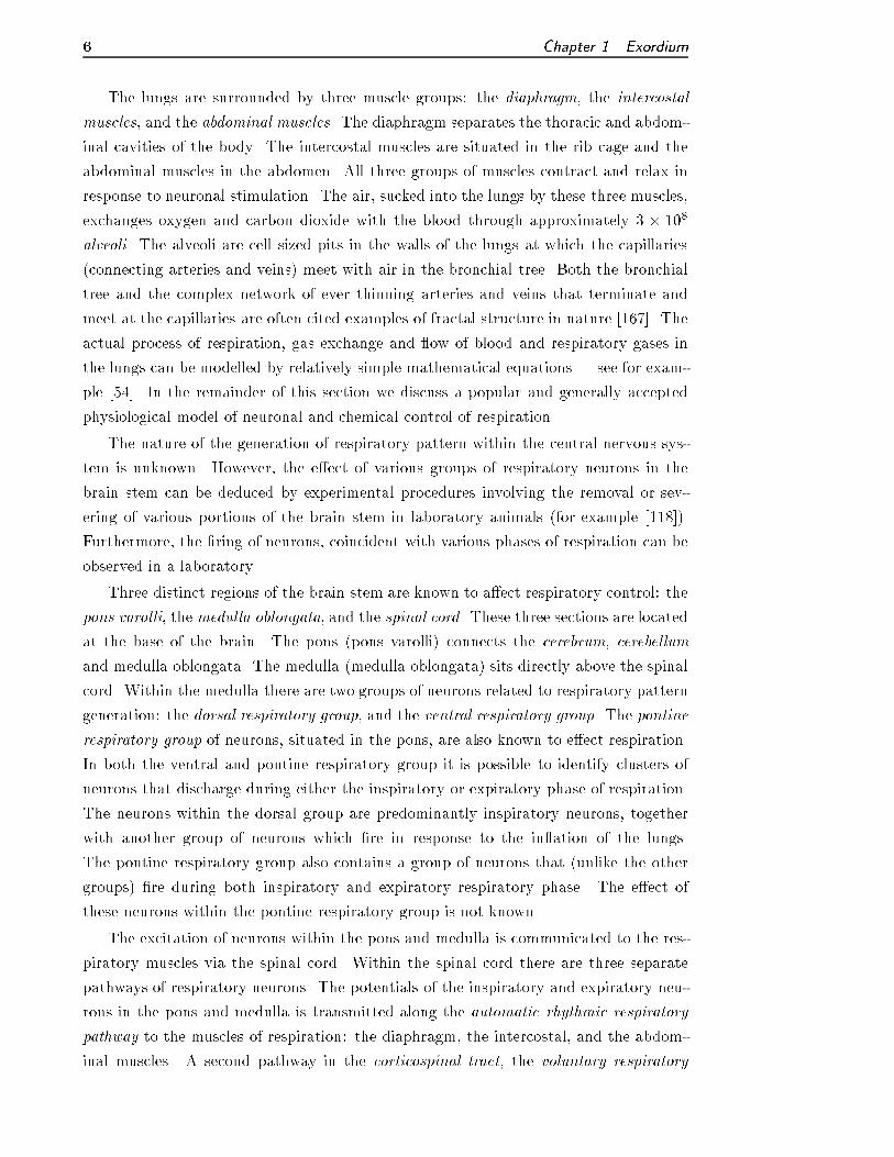
The lungs are surrounded by three muscle groups: the diaphragm, the intercostal
muscles, and the abdominal muscles. The diaphragm separates the thoracic and abdom-
inal cavities of the body. The intercostal muscles are situated in the rib cage and the
abdominal muscles in the abdomen. All three groups of muscles contract and relax in
response to neuronal stimulation. The air, sucked into the lungs by these three muscles,
exchanges oxygen and carbon dioxide with the blood through approximately 3 � 108
alveoli. The alveoli are cell sized pits in the walls of the lungs at which the capillaries
(connecting arteries and veins) meet with air in the bronchial tree. Both the bronchial
tree and the complex network of ever thinning arteries and veins that terminate and
meet at the capillaries are often cited examples of fractal structure in nature [167]. The
actual process of respiration, gas exchange and ow of blood and respiratory gases in
the lungs can be modelled by relatively simple mathematical equations | see for exam-
ple [54]. In the remainder of this section we discuss a popular and generally accepted
physiological model of neuronal and chemical control of respiration.
The nature of the generation of respiratory pattern within the central nervous sys-
tem is unknown. However, the e�ect of various groups of respiratory neurons in the
brain stem can be deduced by experimental procedures involving the removal or sev-
ering of various portions of the brain stem in laboratory animals (for example [118]).
Furthermore, the �ring of neurons, coincident with various phases of respiration can be
observed in a laboratory.
Three distinct regions of the brain stem are known to a�ect respiratory control: the
pons varolli, the medulla oblongata, and the spinal cord. These three sections are located
at the base of the brain. The pons (pons varolli) connects the cerebrum, cerebellum
and medulla oblongata. The medulla (medulla oblongata) sits directly above the spinal
cord. Within the medulla there are two groups of neurons related to respiratory pattern
generation: the dorsal respiratory group, and the ventral respiratory group. The pontine
respiratory group of neurons, situated in the pons, are also known to e�ect respiration.
In both the ventral and pontine respiratory group it is possible to identify clusters of
neurons that discharge during either the inspiratory or expiratory phase of respiration.
The neurons within the dorsal group are predominantly inspiratory neurons, together
with another group of neurons which �re in response to the in ation of the lungs.
The pontine respiratory group also contains a group of neurons that (unlike the other
groups) �re during both inspiratory and expiratory respiratory phase. The e�ect of
these neurons within the pontine respiratory group is not known.
The excitation of neurons within the pons and medulla is communicated to the res-
piratory muscles via the spinal cord. Within the spinal cord there are three separate
pathways of respiratory neurons. The potentials of the inspiratory and expiratory neu-
rons in the pons and medulla is transmitted along the automatic rhythmic respiratory
pathway to the muscles of respiration: the diaphragm, the intercostal, and the abdom-
inal muscles. A second pathway in the corticospinal tract, the voluntary respiratory

1.1. Dynamics of respiration 7
pathway is associated with voluntary (conscious) respiratory action. A third pathway,
the automatic tonic respiratory pathway, located adjacent to the automatic rhythmic
respiratory pathway, has unknown e�ect.
This completes a discussion of the transmission from brain stem to lung of the respi-
ratory pattern. However, the system is further complicated by a form of feedback loop.
The vagus (or vagal nerve) is the tenth (of twelve) major cranial nerves and originates
from the medulla oblongata. The vagal nerve splits into thirteen branches including
the bronchial, superior laryngeal, and recurrent laryngeal nerves which terminate at the
bronchi, the larynx, and the pharynx respectively. Pulmonary stretch receptors located
in the bronchi and trachea sense the state of muscle tone, and therefore air ow, in
these areas. This information is transmitted, indirectly, back along the vagus to the
brain stem and the respiratory motor neurons located there. The phenomenon of the
vagus as a form of feedback mechanism is well known, its exact e�ect is not. Sammon
[118] has shown that the correlation dimension of respiratory activity decreases in rats
after vagotomy.
In addition to feedback via the vagal nerve of information concerning air ow in the
trachea the respiratory system receives input from other sources including the peripheral
arterial chemoreceptors. The peripheral arterial chemoreceptors are located on the
common carotid artery at the point where it splits into two. The carotid artery is
connected via the aorta to the left ventricle of the heart. These chemoreceptors measure
the concentration of oxygen in the blood and transmit this information to the respiratory
pattern generator in the brain stem. There are also many other e�ects on respiration
including, for example, temperature dependent e�ects which have been hypothesised to
be related to incidence of sudden infant death [33].
Hence, the �ring of neurons in the pons and medulla generate potentials that are
transmitted through the spinal cord to the muscle surrounding the lungs. The lungs,
acting as a set of bellows draw air into and expel it from them. Whilst in the lungs,
oxygen is absorbed from the air and carbon dioxide is disgorged from the blood. The air
ow through the bronchi and trachea, and the oxygen concentration in the blood e�ect
pulmonary stretch receptors and chemoreceptors. These receptors indirectly transmit
this information via the vagus back to neurons in the brain stem. Additional information
concerning the environment and the state of activity of an individual also, indirectly
act on the respiratory motor neurons in the brain stem.
The exact manner in which respiratory pattern is generated in the central nervous
system is not known. The purpose of the automatic tonic respiratory pathway in the
spinal column and some groups of respiratory neurons in the pons and medulla are also
unknown.
1.1.2 Pathology Finally, we move from a discussion of control of respiration to
highlight several important phenomena often evident in infants. The �rst is periodic

8 Chapter 1. Exordium
0 50 100 150 200−2
0246
time (sec.)
Ms2t4
Figure 1.2: Periodic breathing: An example of periodic breathing in an infant. At
approximately 110 seconds the respiratory pattern switches from regular quiet breathing
to periodic breathing.
or Cheyne-Stokes breathing. Periodic breathing is the regular periodic uctuation in
the amplitude of respiration from zero to normal respiratory levels. This phenomenon
typically occurs over a period of 10{20 seconds and is common during sleep for healthy
infants. There is, however, some evidence that infants with near miss sudden infant
death have abnormally high levels of periodic breathing [66].
Secondly, sleep apnea is the cessation of breathing for a period of several seconds
during natural sleep. There are two distinct types of apnea, central apnea and obstructive
apnea. Central apnea is caused by the muscles of the lungs stopping the normal rhythm
because of lack of input from the neural pattern generator. Obstructive sleep apnea is
caused by a blockage of the airway and is often associated with snoring. Central apnea
is of far greater relevance to a study of the control of breathing. Again, short apneaic
episodes are not uncommon in normal, healthy infants. Some factors that have been
shown to contribute to increased apnea include an increase body temperature and sleep
deprivation [40].
Finally, bronchopulmonary dysplasia (BPD) is a common phenomenon among in-
fants | particularly as a complication in the treatment of respiratory distress syndrome
(RDS). Respiratory distress syndrome is caused by an infant being born whilst the respi-
ratory system is still incapable of functioning outside the womb. This is usually treated
with forms of arti�cial respiration, respiratory aids or the administration of oxygen. A
common side e�ect of this treatment is bronchopulmonary dysplasia. Infants exhibiting
bronchopulmonary dysplasia will generally have respiratory di�culty and insu�cient
oxygenation of the blood [72].
1.1.3 Chaos and physiology As �gure 1.1 demonstrates there is a plethora
of publications on various applications of dynamical systems theory in general, and
correlation dimension speci�cally, to physiological systems. In this section we do not
o�er a complete review of this literature. Instead we present a representative selection
of publications across the �elds of medicine and physiology along with some more exotic

1.1. Dynamics of respiration 9
applications.
The majority of papers published in this �eld | especially less recent publications |
concentrate on the estimation of correlation dimension, or some variant. Particularly, in
electroencephalography and clinical neurophysiology correlation dimension has become
a common tool of analysis, for example [3, 10, 52, 87, 94, 105, 111, 112, 146, 151, 154].
In particular, the paper of Theiler [151] and Theiler and Rapp [154] o�ers a critical
appraisal of the techniques of dimension estimation and the application of surrogate
data techniques. Birbaumer and others [10] have compared correlation dimension es-
timates of electroencephalogram signals whilst listening to classical and contemporary
music | and concluded that classical music generates a response with higher correlation
dimension.
There is also large number of publication on the analysis of electrocardiographic
signals [9, 38, 39, 56, 88, 128, 129, 132, 147, 156, 158, 168]. A paper from Storella and
colleagues [147] gives a simple demonstration of the e�ectiveness of these techniques. In
this paper, Storella and colleagues show that the response of complexity and variance
of heart rate variability to anaesthesia are di�erent and demonstrate the complexity
is more sensitive to changes in the cardiovascular system than heart rate variability.
Gar�nkel and others [38, 39] have demonstrated an e�ective method for controlling
cardiac arrythmias induced in rabbits. The implications of these methods for patients
with heart conditions is signi�cant [22]. Estimation of correlation dimension has also
found application in the analysis of uctuations in blood pressure [165], characterising
the behaviour of the olfactory bulb [130, 131], and in analysis of optokinetic nystagmus
[123], parathyroid hormone secretion [100] and diastolic heart sounds [91]. Ikeguchi and
colleagues have analysed the dimensional complexity of Japanese vowel sounds [58].
Apart from correlation dimension estimation other studies have estimated the en-
tropy of physiological process [83, 96] and the entropy of rat movement in a con�ned
space [93]. Lippman and colleagues [78, 79] have applied the techniques of nonlinear
forecasting to electrocardiogram signals. Using these methods they \clean" the electro-
cardiographic data of abnormal heart beats [78], and apply nonlinear forecasting as a
form of characterisation of electrocardiograms [79]. Hoyer and others [56] also apply
methods of nonlinear prediction.
Of course, there is also a substantial amount of literature concerning the analysis of
respiratory signals using the techniques of nonlinear dynamical systems theory [16, 17,
23, 32, 35, 95, 114, 115, 116, 117, 118, 166].
Donaldson [23] used estimates of Lyapunov exponents to conclude that resting respi-
ration is chaotic. However, this study was unable to distinguish a nonlinear dynamical
system from linearly �ltered noise.
Pilgram [95] presents an analysis of correlation dimension estimates during REM
sleep and utilises linear surrogate techniques. This study concluded that breathing
during REM sleep is chaotic.

10 Chapter 1. Exordium
Webber and Zbilut [166] demonstrate the application of recurrence plot techniques
to respiratory and skeletal motor data.
Cleave and colleagues [16, 17] present a theoretical analysis of the respiratory re-
sponse to a sigh [16], and demonstrate the existence of a Hopf bifurcation in a feedback
model of respiration [17]. A similar analysis of the response of the respiratory sys-
tem to sighs [32] �tted a second order damped oscillator to response curves. Fowler
and colleagues [35] have proposed a singular value decomposition type method to �lter
respiratory oscillations.
Sammon and colleagues [114, 115, 116, 117, 118] give a comprehensive analysis of
respiration in rats and the e�ect of vagotomy on this respiration. From their observa-
tions they concluded that, in anaesthetised, vagotomised, rats the respiratory system
behaves as an oscillator with a single degree of freedom. With the vagus intact however,
respiratory behaviour was more complex, exhibiting low-order chaos which the authors
speculated, was due to feedback from various types of pulmonary a�erent activity.
1.1.4 Mathematical models of respiration The simplest models of the respi-
ratory system are those of gas exchange in the lungs [54]. One can model the absorption
of oxygen into, and the excretion of carbon dioxide from the blood in the lungs. These
models are based on the ideal gas law, rates of absorption and solubility between gas
and liquid, and conservation of matter. These simple equations provide a good model
of the exchange between gases in air and blood in the lung. Models of the control of
respiration which explain observable phenomena such as periodic breathing are more
sophisticated.
Fundamental to many such models is an oscillatory driving signal, a group of neurons
or a cerebral control centre. This provides the driving force for the respiratory motion.
Such a model was proposed by van der Pol in 1926 [157] 2 and latter generalised [31].
Some form of periodic orbit, or Hopf bifurcation (for example [17]), is central to many
models of respiration.
The Mackey-Glass equations [81] are �rst order delay di�erential equations which
model physiological systems. These equations were proposed in a general context and
were shown to exhibit qualitative features of respiration, including Cheyne-Stokes res-
piration (periodic breathing). An extension to this system which takes into account the
cerebral control centre driving respiration has also been shown to provide similar results
[74].
Sammon [114] gives a detailed analysis of a second order ordinary di�erential equa-
tion for the central respiratory pattern generator and shows that the eigenvalues of a
�xed point of that system can generate a variety of behaviours consistent with respi-
ration. In another paper Sammon presents a more complex multivariate model of the
2Van der Pol's discussion was in the general context of \relaxation oscillators, particularly in electric
circuits and cardiac rhythm.

1.1. Dynamics of respiration 11
respiratory pattern generator [115]. Others have proposed damped oscillator models of
the respiratory response to a sigh [16, 32] and feedback models of the respiratory system
[17].
In a series of papers Levine, Cleave and colleagues [16, 17, 77, 76] have proposed
successive di�erential equation models of the respiratory system. Their simplest model
[16, 17] incorporated blood gas concentration feedback and was represented by three
di�erential equations. This model exhibited Hopf bifurcations under some circumstance
[17]. Subsequent models incorporated �ve [77] and eight [76] di�erential equations.
These models indicate that periodic breathing was a consequence of small changes in
model parameters, and may be a reaction to hypoxic conditions. Decreased oxygenation
was shown to trigger the onset of periodic breathing.
The majority of work in modelling respiration appears in the bioengineering liter-
ature, [68] provides an overview of some recent developments. Many of these studies
model the concentration of gases in blood and not the respiratory motion of the lungs.
Hoppensteadt and Waltman [55] proposed a model of carbon dioxide concentration in
blood which was able to mimic some qualitative features of Cheyne-Stokes breathing. A
similar model of carbon dioxide concentration was also reported by Vielle and Chauvet
[159]. Cooke and Turi [20] have suggested a simple delay equation model of respira-
tory control and present an analysis of that model of the respiratory control system.
A control system model of respiration is also described by Longobardo and colleagues
[80]. This model was able to reproduce some qualitative features of sleep apnea and
Cheyne-Stokes breathing. Grodins and colleagues [46] describe a complex series of di�er-
ential and di�erence equations modelling gas transportation and exchange, blood ow,
and ventilatory behaviour. A computer implementation of these equations was able to
produce some qualitative features of the respiratory system. Finally, Khoo and others
[69, 70] have presented general models of periodic breathing as a result of respiratory
instability.
All these models are based on equations governing various physical processes. These
equations are determined by the investigators and based on what they consider ap-
propriate characteristics of the system. However, the respiratory system, its neuronal
control and the e�ect of other external and internal forces is doubtless more compli-
cated than any of these models. Our approach is somewhat di�erent. We use a model
construction method based upon the fundamental theorems of Takens (see section 2.1).
By assuming the presence of a Markov process other authors have constructed hidden
Markov models [26, 71] of data. Coast and colleagues [18, 19] have applied hidden
Markov models to electrocardiographic signals during arrhythmia. By building hidden
Markov models of di�erent types of beats exhibited by the electrocardiogram signals
of one subject they were able to calculate the most likely model for a given (new)
beat and use this to classify heart beats. Radons and colleagues [106] have applied
similar methods to the analysis of electroencephalogram measurements of a monkey's

12 Chapter 1. Exordium
visual cortex. In this study hidden Markov models were used to classify the response to
di�ering visual stimuli of a 30 electrode array implanted in a monkey's visual cortex.
Altenatively, nonlinear stochastic time series models with a feedback device may be
employed to model respiratory oscillations. These techniques are described by Priestly
[103]. Priestly connects a threshold autoregressive process and bilinear models using
feedback. These techniques may adequately mimic the irregular almost periodic oscil-
lations observed in respiratory oscillations.
An approach similar to those described above could be employed here, however we
do not employ these methods but build radial basis models. Radial basis models are
more compliant to the techniques of nonlinear dynamical systems theory. There have
been many published works demonstrating the application of the radial basis modelling
techniques utilised in this thesis, to dynamical systems theory. Judd and Mees [62]
demonstrate the application of radial basis modelling to the modelling of sunspot dy-
namics. In a very recent paper [64] they apply radial basis modelling techniques to
model sunspot dynamics and Japanese vowel sounds. Cao, Mees and Judd [13] have
demonstrated the application of these method to modelling and predicting with non-
stationary time series. Finally, Judd and Mees [63] demonstrates the presence of a
Shil'nikov bifurcation [124, 125, 126] mechanism in the chaotic motion of a vibrating
string.
1.1.5 Periodic respiration In section 1.1.2 we described the physiological phe-
nomenon known as periodic breathing. In chapter 9 we will introduce a new technique
to detect faint periodic patterns in noisy time series and demonstrate that cyclic uc-
tuations in the amplitude of respiration during normal quiet sleep is a ubiquitous phe-
nomenon. Hence it is relevant at this stage to brie y review other researchers e�orts to
detect cyclic uctuation in the amplitude of respiration.
Fleming and co-workers [32, 34] demonstrated age dependent periodic uctuation
in amplitude in response to a spontaneous sigh in infants. This was achieved by �tting
di�erential equations modelling a decaying oscillator to the experimentally measured
response. They found that the period of oscillations increased with age and the damping
increases then decreases.
Brusil, Waggener and colleagues [11, 12, 162, 160, 164, 161] applied a comb �lter
technique to detect periodic uctuations of amplitude in the respiration of adults at
simulated extreme altitude [12, 160] and in premature infants [162, 164, 161]. They
found that in premature infants the period of uctuations was related to the duration
of apnea. The comb �lter technique they applied was a series of course grained band pass
�lters applied to a synthetic signal derived from abdominal cross-section recordings. The
comb �lter is e�ectively equivalent to a frequency averaged Fourier spectral estimate.
In another series of studies Hathorn [49, 50, 51] investigated periodic changes in
ventilation of new born infants (less than one week old). Hathorn applied Fourier

1.1. Dynamics of respiration 13
spectral and autocorrelation estimates to quantify amplitude and frequency uctua-
tions. Furthermore, using a sliding window technique they investigated the e�ects of
non-stationarity. By splitting the frequency components of ventilation into high and
low frequency Hathorn showed a stronger coherence between respiratory oscillations
and heart rate in quiet sleep [51]. Hathorn's investigations were based on analysis of
time/breath amplitude analysis whereas the analysis we perform in this thesis is of
breath number/breath amplitude data. Furthermore, the infants we examine in this
study vary over a wider range of ages (up to six months).
Finley and Nugent [29] applied spectral techniques to demonstrate that new born
infants exhibit a frequency modulation in normal respiration (during quiet sleep) of
approximately the same frequency as periodic breathing.
A series of other studies by other various groups [30, 43, 75, 101] have also demon-
strated some periodic uctuations in amplitude of respiratory e�ort in either resting
adults [43, 75, 101] or sleeping infants [30].
1.1.6 Motivation The simplest model of respiratory control is described in sec-
tion 1.1.1. Respiration is governed by discrete \pacemaker" cells with intrinsic activity
that drives other respiratory neurons. The output of various respiratory centres or pools
of motor neurons is then organised by a pattern generator. An alternative approach
implies that networks of cells with oscillatory behaviour interact in a complex way to
produce respiratory rhythms which are either further organised by a pattern generator
or might be self-organising [28]. The purpose and behaviour of many groups of neu-
rons in the respiratory control centres and there interaction is still unknown and so this
approach is essentially a further complication of the description given in section 1.1.1.
Advances in neurobiology have allowed recordings to be made from individual neu-
rons and groups of neurons in the brain. Using these techniques, various studies have
demonstrated that the concept of discrete respiratory centres made up of neurons with
speci�c functions de�ned by the nature of a particular \centre" is obsolete [28]. Whilst
there is organisation of neurons into functional networks or pools these are not neces-
sarily anatomically discrete. Also, there are con icting data in regard to the presence
of a speci�c pattern generator. Given the complexity of the connections between the
various groups of oscillating, respiratory-related neurons, and the capacity for inter-
actions between simple oscillating systems to produce complex behaviour, we believe
that information about the organisation of respiratory control can be determined using
dynamical systems theory. In essence, the argument that there is a simple \pattern gen-
erator" that co-ordinates the output from various \respiratory centres" is unnecessary
if the output from interacting networks is dynamical and self-organising.
Other authors have applied techniques derived from dynamical system theory to
respiratory systems with some success. These studies are summarised in sections 1.1.3
and 1.1.4. In particular, Cleave and colleagues [17] have demonstrated the possible

14 Chapter 1. Exordium
existence of Hopf bifurcations in the response of the respiratory system to sighs. Sam-
mon and others [114, 115, 116, 117, 118] give a comprehensive analysis of respiration
in rats using the techniques of dynamical system theory. Numerous other authors have
presented evidence of chaos in correlation dimension and Lyapunov exponent estimates
for respiratory data.
Recent physiological studies [57] have suggested that immature or abnormal devel-
opment of the respiratory control centres in the brain stem may be a contributing factor
to sudden infant death syndrome (SIDS). It is hypothesised [57] that infants at risk of
SIDS do not have a properly developed respiratory control and are therefore unable to
respond to pathological and physiological stresses (such as hypoxia, airway obstruction,
and hypercapnia). However this study has been unable to �nd distinctions between
\normal" and \at risk" infants which can be used to diagnose risk of sudden infant
death. This method has been unable to detect subtle variation between subjects which
the techniques of nonlinear dynamical system theory may.
1.2 Data collection
The experimental protocol of all the studies described in this thesis are basically iden-
tical. For these studies we collected measurements proportional to the cross-sectional
area of the abdomen of infants during natural sleep. To do this we used standard non-
invasive inductive plethysmography techniques which will be described in more detail
latter. Such measurements are a gauge of lung volume. The abdominal signal is not
necessarily proportional to lung volume but the signal is su�cient for our purposes3.
Moreover, present methods are not capable of dealing well with multichannel data and
therefore use of both rib and abdominal signal to approximate actual lung volume is
di�cult. Of the available measurements we found that the abdominal cross section was
the easiest to measure experimentally.
These studies were conducted in a sleep laboratory during day time and overnight
sleep studies at Princess Margaret Hospital for Children4 . These studies had approval
from the ethics committee of Princess Margaret Hospital and the University of Western
Australia Board of Postgraduate Research Studies. The parents of the subjects of these
studies were informed of the procedure, and its purpose, and had given consent.
1.2.1 Experimental methodology An inductance plethysmograph provides a
non-invasive measurement of cross-sectional area. It consists of a thin wire loop wrapped
in an elasticised band. This is placed (in this study) around the abdomen of a sleeping
infant. A small electrical (AC) voltage potential is created at the ends of this wire
3Takens' embedding theorem [148] (and therefore the methods of this chapter, see section 2.1) only
require a C2 (smooth) function of a measurement of the system.4Department of Respiratory Medicine, Princess Margaret Hospital for Children, Subiaco, WA, Aus-
tralia 6008.

1.2. Data collection 15
generating an alternating current in the loop. Voltage v and current { in an inductor
are related by [89]
v =d(L{)
dt(1.1)
where L is the inductance. Inductance in a wire loop is given by [89]
L =�A
`(1.2)
where A and ` are the area enclosed by, and length of, the wire. The permeability � is
a constant electromagnetic property of the medium. Substituting (1.2) into (1.1), one
gets
v =�
`
�dA
dt{+A
d{
dt
�:
Let { = I0 cos (!2�t) where ! is the frequency of the alternating current source, and so,
v =�
`I0
�dA
dtcos
� !
2�t��A
!
2�sin
� !
2�t��
:
Let v = V0 cos (!2�t + �), and a trivial trigonometric identity yields
V0 cos � =�
`I0dA
dt
V0 sin � =�
`I0A
!
2�
and therefore
V0 =�I0
2�`
sA2!2 + 4�2
�dA
dt
�2
: (1.3)
However A! � 2� dAdt
so V0 ��I0A!
2�`. Hence, the magnitude of the current is inversely
proportional to the cross sectional area of the wire loop.
In addition to the inductance plethysmograph, polysomnographic criterion are used
to score sleep state [7]. A polysomnogram consists of a series of separate pieces of
equipment to measure eye movement, brain activity, respiration, muscle movement and
blood gas concentrations. Typically a polysomnogram consists of electroencephalogram
(EEG), electrooculogram (EOG), electromyogram (EMG) and electrocardiogram (ECG)
to measure brain activity, eye movement, muscle tone and heart rate. An oximeter
is employed to measure blood oxygen saturation (the concentration of oxygen in the
blood), nasal and oral thermistors measure temperature change at nose and mouth
(this is related to the quantity of air exhaled), and plethysmography is used to record
rib and abdominal movement. For a detailed discussion of sleep studies see [85].
The un�ltered analogue signal from the inductance plethysmograph5 is passed
through a DC ampli�er and 12 bit analogue to digital converter (sampling at 50Hz).
5Non-invasive Monitoring systems, (NIMS) Inc; trading through Sensor medics, Yorba Linda, CA.,
USA.

16 Chapter 1. Exordium
The digital data were recorded in ASCII format directly to hard disk on an IBM com-
patible 286 microcomputer using LABDAT and ANADAT software packages6. These
data were then transferred to Unix workstations at the University of Western Australia
for analysis using MATLAB7 and C programs.
By amplifying the output of the inductance plethysmograph before digitisation our
data occupy at least 10 bits of the AD convertor. Hence, error due to digitisation is less
than 2�11 < 0:0005. Errors due to the approximation involved in the derivation of (1.3)
are substantial less than digitisation e�ects. Our data are sampled at 50Hz, however,
tests at higher sampling rates indicate that there is no signi�cant aliasing e�ect.
The only practical limitation on the length of time for which data could be collected
is the period that the infant remains asleep and still. The cross sectional area of the
lung varies with the position of the infant. However, in this study we are interested
only in the variation due to the breathing and so we have been careful to avoid artifact
due to changes in position or band slippage. We have made observations of up to two
hours that are free from signi�cant movement artifacts, although typically observations
are in the range �ve to thirty minutes.
1.2.2 Data The data collected for this thesis consists primarily of two sections.
A longitudinal study was conducted with nineteen healthy infants studied at 1, 2, 4 and
6 months of age. These studies were performed exclusively during the day. Data from
this study we designate as group A.
In a separate study, a group of 32 infants and young children admitted to Princess
Margaret Hospital were studied during overnight sleep studies arranged for other pur-
poses. Of these subjects 28 were under 24 months of age. Most were su�ering from
either bronchopulmonary dysplasia (8 of 32) or central (13) or obstructive (4) sleep
apnea. These data are subdivided according to the clinical reasons for the sleep study.
Infants su�ering from clinical apnea we designate as group B, those with bronchopul-
monary dysplasia we designate as group C, the remainder are group D.
1.3 Thesis outline
This thesis is organised into four separate parts: (I) this introduction; (II) a summary
of the required mathematical background; (III) the analysis of infant respiration; and
(IV) the conclusion.
Part II contains two chapters, chapter 2 covers background material from the �eld
of nonlinear dynamical systems theory. Chapter 2 describes general reconstruction
techniques, Takens' embedding theorem, correlation dimension, correlation dimension
estimation, and radial basis modelling. The second part of this summary, chapter 3,
6RHT-InfoDat, Montreal, Quebec, Canada.7The Math Works, Inc., 24 Prime Park Way, Natick, MA., USA.

1.3. Thesis outline 17
describes the method of surrogate data and summarises some terminology and theory
commonly applied in the literature.
Part III is the dynamical systems analysis of respiration in human infants during
natural sleep. This part describes the methods employed, the theory developed and the
results obtained. All of the new results of this thesis are described in this part. Part III
of the thesis is split into eight chapters.
Chapter 4 concerns surrogate data techniques. This chapter describes various meth-
ods of surrogate generation and provides some comparison between them. Some general
theory concerning the pivotalness of correlation dimension estimates is developed and
some numerical calculations con�rming these results is presented. In this chapter we
present a new result concerning the conditions which ensure a test statistic is pivotal.
Using this result we show many statistics based on dynamical system theory are asymp-
totically pivotal. In particular, we demonstrate that correlation dimension estimated
using the algorithm described by Judd [60, 61] provides a pivotal test statistic for classes
of linear and nonlinear surrogates.
In chapter 5 we provide a brief summary of the application of various methods de-
scribed in section 2.1 to choose the parameters of time delay embeddings. The results
of this section are primarily concerned with demonstrating the estimation of embedding
parameters for respiratory data using existing techniques. For two dimensional embed-
dings we apply a novel approach to demonstrate the dependence on the shape of the
embedded data on embedding parameters. We use this to suggest an appropriate value
of embedding lag.
The modelling methods developed for this thesis are discussed in chapter 6. This
chapter also describes the e�ectiveness of the modelling method employed. This chapter
develops the necessary theory and methodology to describe the modelling methods we
employ. We show that successive alterations to an earlier modelling algorithm eventually
produce models which exhibit many qualitative and quantitative similarities to data.
The modelling algorithm is based on methods discussed by Judd and Mees [62], however
the application of this algorithm to respiratory recordings and the alterations to this
algorithm are original. Using these new improvements to this existing algorithm we are
able to demonstrate CAM during quiet breathing and show that it has the same period
as periodic breathing following a sigh.
Chapter 7 describes, in more detail, some results of the application of the modelling
methods of chapter 6. This chapter analyses the nature of the dynamics present in
the models of respiratory data and presents evidence of period doubling bifurcations
in some models of infant respiration. Evidence of stretching and folding of trajectories
is also presented. The results presented in this chapter are a new application of ex-
isting techniques of dynamical systems theory to the analysis of nonlinear models. By
analysing properties of cylindrical basis models we are able to infer characteristics of
the dynamical system which generated the observed data.

18 Chapter 1. Exordium
The results of chapter 8 are based largely on a paper published in the physiological
literature. This chapter describes the analysis of infant respiration using the tools we
have developed and described so far. We use correlation dimension estimation, linear
and nonlinear surrogate analysis and cylindrical basis modelling to conclude that infant
respiration is likely to be a two to three dimensional system with at least two periodic
(or quasi-periodic) driving mechanisms and additional complexity. Furthermore, this
system is modelled well by the cylindrical basis modelling methods we describe. The
application of these methods to the analysis of infants respiration and the conclusions
we reach are new.
Chapter 9 describes calculations to detect this second periodic source (the cyclic
amplitude modulation) present in the infant respiratory system. This chapter em-
ploys new linear modelling techniques derived from the nonlinear modelling methods
described in chapter 6 and information theoretic measurement of \structure" described
in that chapter. These calculations detect the presence of a cyclic amplitude modula-
tion of approximately the same period as periodic breathing and we conclude that this
phenomenon represents a ubiquitous driving mechanism present during regular respira-
tion but most notable only during periodic breathing. This is the �rst evidence of the
presence of CAM during quiet respiration in all infants.
Finally, chapter 10 describes the application of nonlinear methods: Floquet theory
and Poincar�e sections to detect cyclic amplitude modulation from models of respira-
tion. The results of this chapter con�rm an earlier assertion that the respiratory system
exhibits a periodic, or quasi-periodic amplitude modulation. In data where cyclic am-
plitude modulation is not evident the �rst return map exhibits a stable focus.
The �nal part of this thesis contains one section and is a summary and conclusion.

19
Part II
Techniques from dynamical
systems theory


21CHAPTER 2
Attractor reconstruction from time series
In this chapter we describe the reconstruction of an unknown dynamical system from
data. The general techniques described here may be found in many references: [2]
discusses reconstruction techniques and [98] is a summary of radial basis modelling
techniques. In section 2.1 we describe attractor reconstruction and Takens' embedding
theorem. Section 2.2 is a discussion of correlation dimension estimation and section 2.3
is concerned with radial basis modelling and description length [110]. In chapter 3 we
will review existing hypothesis testing methods using surrogate data.
2.1 Reconstruction
Attractor reconstruction using the method of time delays is now widely applied, we
will brie y describe the key points of this technique and the methods we utilise to select
an appropriate embedding strategy.
Let M be a compact m dimensional manifold, Z : M 7�! M a C2 vector �eld on
M , and h : M 7�! R a C2 function (the measurement function). The vector �eld
Z gives rise to an associated evolution operator ( ow) �t : M 7�! M . If zt 2 M is
the state at time t then the state at some latter time t + � is given by zt+� = �� (zt).
Observations of this state can be made so that at time t we observe h(zt) 2 R and at
time t+ � we can make a second measurement h(�� (zt)) = h(zt+� ). Taken's embedding
theorem [148] guarantees that given the above situation, the system generated by the
map �Z;h : M 7�! R2m+1 where
�Z;h(zt) := (h(zt); h(��(zt)); : : : ; h(�2m�(zt))) (2.1)
= (h(zt); h(zt+�); : : : ; h(zt+2m�))
is an embedding. By embedding we mean that the asymptotic behaviour of �Z;h(zt) and
zt are di�eomorphic.
We can apply this result to reconstruct from a time series of experimental observa-
tions fytgNt=1 (where yt = h(zt)) a system which1 is (asymptotically) di�eomorphic to
that which generated the underlying dynamics. We produce from our scalar time series
y1; y2; y3; : : :; yN
a de-dimensional vector time series via the embedding (2.1)
yt�� 7�! vt = (yt�� ; yt�2� ; : : : ; yt�de�) 8t > de�:
To perform this transformation one must �rst identify the embedding lag � and the em-
bedding dimension de2. We describe the selection of suitable values of these parameters
1Subject to the usual restrictions of �nite data and observational error.2A su�cient condition on de is that it must exceed 2m + 1 where m is the attractor dimension.
However, to estimatem, one must already have embedded the time series. Any values of � is theoretically
acceptable, however, for �nite noisy data it is preferable to select an \optimal" value.

22 Chapter 2. Attractor reconstruction from time series
in the following paragraphs.
An embedding depends on two parameters, the lag � and the embedding dimen-
sion de. For an embedding to be suitable for successful estimation of dimension and
modelling of the system dynamics, one must choose suitable values of these parame-
ters. The following two subsections discuss some commonly used methods to estimate
embedding lag � and embedding dimension de.
2.1.1 Embedding dimension de Takens embedding theorem [90, 148] and more
recently work of Grebogi [21]3 give su�cient conditions on de. Unfortunately, the con-
ditions require a prior knowledge of the fractal dimension of the object under study.
In practice one could guess a suitable value for de by successively embedding in higher
dimensions and looking for consistency of results; this is the method that is generally em-
ployed. However, other methods, such as the false nearest neighbour technique [27, 150],
are now available to suggest the value of de.
False Nearest Neighbours Suitable bounds on de can be deduced by using false near-
est neighbour analysis [67]. The rationale of false nearest neighbour techniques is the
following. One embeds a scalar time series yt in increasingly higher dimensions, at each
stage comparing the number of pairs of vectors vt and vNNt (the nearest neighbour of
vt) which are close when embedded in Rn but not close in Rn+1. Each point
vt = (yt�� ; yt�2� ; : : : ; yt�n� )
has a nearest neighbour
vNNt = (yt0�� ; yt0�2� ; : : : ; yt0�n� ):
When one has a large amount of data the distance (Euclidean norm will do) between vt
and vNNt should be small. If these two points are genuine neighbours then they became
close due to the system dynamics and should separate (relatively) slowly. However,
these two points may have become close because the embedding in Rn has produced
trajectories that cross (or become close) due to the embedding and not the system dy-
namics4. For each pair of neighbours vt and vNNt in Rn one can increase the embedding
dimension by one so that
bvt = (yt�� ; yt�2� ; : : : ; yt�n� ; yt�(n+1)�)
and
dvNNt = (yt0�� ; yt0�2� ; : : : ; yt0�n� ; yt0�(n+1)� )
3Grebogi gives a su�cient condition on the value of de necessary to estimate the correlation dimension
of an attractor, not to avoid all possible self intersections.4The standard example is the embedding of motion around a �gure 8 in two dimension. At the
crossing point in the centre of the �gure trajectories cross. However, one can imagine if this was
embedded in three dimensions then these trajectories may not intersect.

2.1. Reconstruction 23
may or may not still be close. The increase in the distance between these two point is
given only by the di�erence between the last components
kbvt � dvNNt k2 � kvt � vNN
t k2 = (yt�(n+1)� � yt0�(n+1)� )2:
One will typically calculate the normalised increase to the distance between these two
points and determine that two points are false nearest neighbours if
jyt�(n+1)� � yt0�(n+1)� j
kvt � vNNt k
� RT :
A suitable values of RT depends on the spatial distribution of the embedded data vt.
If RT is too small then true near neighbours will be counted as false, if RT is too large
then some false near neighbours will not be included. Typically 10 � RT � 30, the
calculations in this thesis all have a value of RT = 15. One must ensure that the chosen
value of RT is suitable for the spatial distribution of the data under consideration |
this may be done by trialling a variety of values of RT . By determining if the closest
neighbour to each point is false one can then calculate the proportion of false nearest
neighbours for a given embedding dimension n.
We can then choose as the embedding dimension de the minimum value of n for which
the proportion of points which satisfy the above condition is below some small threshold.
In this thesis we set this threshold to be 1%, however, this value is entirely arbitrary.
Typically one could expect the proportion of points satisfying this to gradually decrease
as the embedded data is \unfolded" in increasing embedding dimension and eventually
plateau at a relatively low level.
2.1.2 Embedding lag � Any value of � is theoretically acceptable, but the shape
of the embedded time series will depend critically on the choice of � and it is wise to
select a value of � which separates the data as much as possible. One typically is
concerned with the evolution of the dynamics in phase space. By ensuring that the
data are maximally spread in phase space the vector �eld will be maximally smooth.
Spreading the data out minimises possibly sharp changes in direction amoungst the
data. From a topological view-point, spreading data maximally makes �ne features of
phase space (and the underlying attractor) more easily discernible.
General studies in nonlinear time series [2] suggest the �rst minimum of the mutual
information criterion [102, 110], the �rst zero of the autocorrelation function [104] or
one of several other criteria to choose � . Our experience and numerical experiments
suggest that selecting a lag approximately equal to one quarter of the approximate
period of the time series produce comparable results to the autocorrelation function
but is more expedient. Note that the �rst zero of the autocorrelation function will be
approximately the same as one quarter of the approximate period if the data are almost
periodic. Numerical experiments with these data show that either of these methods
produce superior results to the mutual information criterion (MIC). We will consider
each of these methods in turn.

24 Chapter 2. Attractor reconstruction from time series
Autocorrelation De�ne the sample autocorrelation of a scalar time series yt of N
measurements to be
�(T ) =
PNn=1(yn+T � �y)(yn � �y)PN
n=1(yn � �y)2
where �y = 1N
PNn=1 yn is the sample mean. The smallest positive value of T for which
�(T ) � 0 is often used as embedding lag. For data which exhibits strong periodic
component it suggests a value for which the successive coordinates of the embedded
data will be virtually uncorrelated whilst still being close (temporally). We stress that
a choice of T such that the sample autocorrelation is zero is purely prescriptive. Sample
autocorrelation is only an estimate of the autocorrelation of the underlying process,
however the sample autocorrelation is su�cient for estimating time lag.
Mutual information A competing criterion relies on the information theoretic con-
cept of mutual information, the mutual information criterion (MIC). In the context of
a scalar time series the information I(T ) can be de�ned by
I(T ) =NXn=1
P (yn; yn+T ) log2P (yn; yn+T )
P (yn)P (yn+T );
where P (yn; yn+T ) is the probability of observing yn and yn+T , and P (yn) is the proba-
bility of observing yn. I(T ) is the amount of information we have about yn by observing
yn+T , and so one sets � to be the �rst local minima of I(T ).
Approximate period The rationale of these previous two methods is to choose the
lag so that the coordinate components of vt are reasonably uncorrelated while still being
\close" to one another. When the data exhibit strong periodicity | as is the case with
respiratory patterns | a value of � that is one quarter of the length of the average
breath generally gives a good embedding. This lag is approximately the same as the
time of the �rst zero of the autocorrelation function. Coordinates produced by this
method are within a few breaths of each other (even in relatively high dimensional em-
beddings) whilst being spread out as much as possible over a single breath. Moreover,
for embedding in three or four dimensions (as will be suggested by false nearest neigh-
bour techniques) the data are spread out over one half to three quarters of a breath.
This means that the coordinates of a single point in the three or four dimensional vector
time series vt represents most of the information for an entire breath. This choice of
lag is extremely easy to calculate and for the data sets that we consider it also seems
to give much more reliable results than the mutual information criterion.
2.2 Correlation dimension
We are accustomed to thinking of real world objects as one, two or three dimen-
sional. However, there exist complex mathematical objects, called fractals, that have
non-integer dimension, a so called fractal dimension. Many real world phenomena, in

2.2. Correlation dimension 25
particular chaotic dynamical systems, can be observed to have properties of a frac-
tal, including a non-integer dimension. A meaningful de�nition of fractal dimension
comes from a generalisation, or extension, of well known properties of integer dimension
objects.
Most applications of correlation dimension to physiological sciences have utilised the
Grassberger and Procaccia algorithm. However, in this thesis we employ a new algo-
rithm, which is technically more complex, but is in practice more reliable and less prone
to misinterpretation. Unlike previous estimation methods this new algorithm recog-
nises that the dimension of an object (its structural complexity) may vary depending
on how closely you examine it. Hence the value of the estimate of correlation dimension
may change with scale. It therefore o�ers a more informative and accurate estimate of
dimension.
Computing correlation dimension dc as a function of scale dc("0) can tell us much
more about the structure of an object, for example, it can indicate the presence of large
scale \periodic" motion and simultaneously detect smaller scale, higher dimensional,
\chaotic" motion and noise. Quoting a single number as the correlation dimension of
a data set ignores much of this information, in many respects it produces an \average
dimension". Plots of dimension as a function of scale are particularly important when
studying complex physiological behaviour because they yield far more information than
a single estimate at a �xed scale.
2.2.1 Generalised dimension Once we have embedded the data properly we
wish to measure the complexity of the \cloud" of points vt. The measure we use in this
paper is the correlation dimension.
We de�ne the correlation dimension by generalising the concept of integer dimension
to fractal objects with non-integer dimension. In dimensions of one, two, three or more
it is easily established, and intuitively obvious, that a measure of volume V (") (e.g.
length, area, volume and hyper-volume) varies as
V (") / "d; (2.2)
where " is a length scale (e.g. the length of a cube's side or the radius of a sphere) and
d is the dimension of the object. For a general fractal it is natural to assume a relation
like equation (2.2) holds true, in which case its dimension is given by,
d �logV (")
log ": (2.3)
Let fvtgNt=1 be an embedding of a time series in Rde . De�ne the correlation function,
CN ("), by
CN (") =
�N
2
��1 X0�i<j�N
I(kvi � vjk < "): (2.4)

26 Chapter 2. Attractor reconstruction from time series
Here I(X) is a function whose value is 1 if condition X is satis�ed and 0 otherwise, and
k � k is the usual distance function in Rde . The sumP
i I(kvi � vjk < ") is the number
of points within a distance " of vj . If the points vi are distributed uniformly within
an object, then this sum is proportional to the volume of the intersection of a sphere
of radius " with the object and CN(") is proportional to the average of such volumes.
Comparing with equation (2.2) one expects that
CN(") / "dc ;
where dc is the dimension of the object. The correlation integral is de�ned as
limN!1 CN("). De�ne the correlation dimension dc by
dc = lim"!0
limN!1
logCN(")
log ": (2.5)
The curious normalisation of CN (") is chosen so that rather than CN (") being an
estimate of the expected number of points of an object within a radius " of a point,
it is instead an estimate of the probability that two points chosen at random on the
object are within a distance " of each other. The di�erence between the expectation
and the probability is only a constant of proportionality if the points were distributed
uniformly, and this constant vanishes in the limit of equation (2.5). The reason for
choosing the probability rather than the expectation is that the concept of dimension
still makes sense, indeed generalises, to situations where the sample points vi are not
distributed uniformly within the object. For a more detailed discussion of the general
situation, see Judd [60].
2.2.2 The Grassberger-Procaccia algorithm The method most often em-
ployed to estimate the correlation dimension is the Grassberger-Procaccia algorithm
[45]5 . In this method one calculates the correlation function and plots logCN(") against
log ". The gradient of this graph in the limit as "! 0 should approach the correlation
dimension. Unfortunately, when using a �nite amount of data the graph will jump about
irregularly for small values of ". To avoid this one instead looks at the behaviour of this
graph for moderately small ". A typical correlation integral plot will contain a \scaling
region" over which the slope of logCN(") remains relatively constant. A common way
to examine the slope in the scaling region is to numerically di�erentiate (or �t a line to)
the plot of log " against logCN ("). This ought to produce a function which is constant
over the scaling region, and its value on this region should be the correlation dimension
(see Fig. 2.2).
5For example, studies of heart rate [129, 132, 156, 168], electroencephalogram [3, 9, 83, 87, 94,
111, 112], parathyroid hormone secretion [100] and optico-kinetic nystagmus [123] have all utilised the
Grassberger-Procaccia algorithm, or some variant of it.

2.2. Correlation dimension 27
2000 4000 6000 8000 10000 12000−10
0
10
n
x(n)
Data
−10 −5 0 5 10−10
−5
0
5
10
x(n−19)
x(n)
−100
10
−100
10−10
−5
0
5
10
x(n−38)x(n)
x(n−
19)
Figure 2.1: A time lag embedding: One of the data sets used in our calculation,
together with the time lag embedding in 2 and 3 dimensions. The time lag used was 19
data points (380ms).
2.2.3 Judd's algorithm Unfortunately, as Judd [60] points out there are several
problems with this procedure. The most obvious of these is that the choice of the scaling
region is entirely subjective (Fig. 2.2). For many data sets a slight change in the region
used can lead to substantially di�erent results. Judd assumes that locally the attractor
can be modelled as the Cartesian cross product of a bounded connected subset of a
smooth manifold and a \Cantor-like" set. Judd demonstrates that for such objects
(which include smooth manifolds and many fractals), a better description of CN(") is
that for " less than some "0
CN(") � "dcq(");
where q(") is a polynomial of order t, the topological dimension of the set. Consequently
we consider correlation dimension dc as a function of "0 and write dc("0), and call this
the dimension at the scale "0.
The Grassberger-Procaccia method assumes that CN(") / "dc , but this new method
allows for the presence of a further polynomial term that takes into account variations
of the slope within and outside of a scaling region. This new method dispenses with
the need for a scaling region and substitutes a single scale parameter "0. This has
an interesting bene�t. For many natural objects the dimension is not the same at all
length scales. If one observes a large river stone its surface at it largest length scale

28 Chapter 2. Attractor reconstruction from time series
−6 −5 −4 −3 −2 −10
5
10
15
distance
log(
occu
panc
y)
Distribution of interpoint distances
−6 −5 −4 −3 −2 −10
2
4
distance
Derivative
Figure 2.2: Correlation dimension from the distribution of inter-point dis-
tances: The logarithm of the distribution of inter-point distances, and an approxima-
tion to the derivative for one of our sets of data embedded in three dimensions. The
approximate derivative is a smoothed numerical di�erence. This calculation used the
same data set as �gure 2.1, embedded in 3 dimensions with a lag of 19 data points
(380ms). Even with well behaved data and a smooth approximately monotonic distri-
bution of inter-point distances the choice of scaling region is still subjective.

2.3. Radial basis modelling 29
is very nearly two-dimensional, but at smaller length scales one can discern the details
of grains which add to the complexity and increase the dimension at smaller scales.
Consequently, it is natural to consider dimension dc as a function of "0 and write dc("0).
By allowing our dimension to be a function of scale we produce estimates that
are both more accurate and more informative. We avoid some of the approximation
necessary to de�ne correlation dimension as a single number and we can extract more
detailed information about the changes in dimension with scale. For an alternative
treatment of this algorithm see, for example [58]. The issue of \lacunarity" in the
attractor is also considered in [144].
2.3 Radial basis modelling
This section provides a brief overview of radial basis modelling and the methods
utilised in this thesis. In particular the section brie y reviews the methods described
by Judd and Mees [62] to build a radial basis model of variable size from data.
2.3.1 Radial basis functions From a scalar time series fytgNt=1 we embed the
data in Rde� (the values of de and � will be selected as in section 2.1, for reasons which
will become apparent we choose to embed in Rde� notRde) as in the proceeding sections
vt = (yt�1; yt�2; : : : ; yt�de�) 8t > de�:
From this we wish to �t a model f : Rde� 7�! R
yt = f(vt) + �t
where �t � N(0; �2). We assume that the model f captures the dynamics of the un-
derlying system and that the model prediction errors �t can be modelled as additive
Gaussian noise. Assuming additive Gaussian noise is a substantial simpli�cation of the
most general possible situation. Choice of error model is an extremely important is-
sue, and in some situations extremely di�cult. For our purposes the simpli�cation to
additive Gaussian noise is su�cient.
Observe that by using a time-delay embedding the only new component of vt+1 that
the model needs to predict is yt. The general form of the function f is
f(v) =nX
j=1
�j�(kv � cjk)
where � : R+ 7�! R is a �xed function. In this situation f is known as a radial basis
function. For a discussion of radial basis functions and possible choices of � see Powell
[98]. There a several common choices of �, most of which are monotonic decreasing
functions6. We o�er a slight generalisation of the functional form described above by
6With the exception of cubic functions s3. Other commonly used basis functions include Gaussian
e�s2 (these are the foundation of the basis functions employed here) and thin plate splines s
2 log s,
among others.

30 Chapter 2. Attractor reconstruction from time series
including an additional scaling factor, and call a function of the form
f(v) =nX
j=1
�j�(kv � cjk
rj) (2.6)
(where rj > 0) a radial basis function. In general the selection of the parameters �j ,
cj (the centres of the jth basis function) and rj (the radius of that basis function) is
a complex nonlinear optimisation problem. They can however, be selected to minimise
the mean sum of squares prediction error of the model f . The parameter n cannot.
To optimise over the model size n we introduce the information theoretic concept of
description length.
2.3.2 Minimum description length principle Roughly speaking the descrip-
tion length of a particular model of a time series is proportional to the number of bytes
of information required to reconstruct the original time series7. That is, if one was
to transmit a description of the data then the description length of the data is the
compression gained by describing the model parameters and the model prediction error.
Obviously if the time series does not suit the class of models being considered then
the most economical way to do this would be to simply transmit the data. If however,
there is a model that �ts the data well then it is better to describe the model in addition
to the (minor) deviations of the time series from that predicted by the model (see
�gure 2.3). Thus description length o�ers a way to tell which model is most e�ective.
Our encoding of description length is identical to that outlined by Judd and Mees [62]
and follows the ideas described by Rissanen [110]. Roughly speaking the description
length is given by an expression of the form
(Description length) � (number of data)�
log (Sum of squares of prediction errors) +
(Penalty for number and accuracy of parameters) :
The approach of Judd and Mees is to calculate the description length penalty of
the model as the penalty from the parameters �j . The parameters cj and rj are given
at no cost. In section 6.2.3 we address this short coming. For the present discussion
we assume, as Judd and Mees have, that the only parameters required to describe the
model are �j for j = 1; 2; : : : ; k.
Rissanen [110] suggest an optimal encoding for a oating point binary number �j =
0:a1a2a3 : : : anj�2mj . If �j is the j
th model parameter and �j that parameter truncated
to nj binary bits, then the di�erence between �j and �j will be at most �j = 2�nj . We
call �j the precision of the parameter �j . Hence to encode �j we need to encode the
binary mantissa a1a2a3 : : :anj and the exponentmj , two integers. The method employed
by Judd and Mees to encode integers is that suggest by Rissanen. The integer p may be
7To within some arbitrary (possibly the machine) precision.

2.3. Radial basis modelling 31
Des
crip
tion
leng
th (
bits
)
model parameters
Model description length
Description length of
Description length of
Model Size (number of parameters)
modelling errors
Figure 2.3: Description length as a function of model size: A plot of the expected
behaviour of description length as a function of model size k of (see equation (2.13)).
For k = 0 there is no model and the description length of the model prediction errors is
the description length of the data. As k increases the description length of the modelling
error decreases as the model starts to �t the data. The description length of the model
parameters increases as more model parameters are added. Eventually the additional
model parameters are unimportant and do not greatly increase the description length
of the model parameters, at this stage the description length of the modelling errors
approaches zero (in the limit when the system is over determined). The optimal model
should be the model for which the model description length (the sum of the description
lengths of the model parameters and the modelling errors) is minimal.

32 Chapter 2. Attractor reconstruction from time series
encoded in log2 p bits, but to do so one must �rst encode the length of this code. That
is, if one was to send the code for p the receiver of that code needs to be told how long
the code is. But the code length is itself a binary integer and the length of that code
must also be speci�ed. Hence the integer p can be encoded as a code word of length
L�(p) = dlog2 ce+ dlog2 pe+ dlog2 dlog2 pee+ dlog2 dlog2 dlog2 peee+ : : :
bits. This sequence continues until the last term is either 0 or 1, dxe is the smallest
integer not less than x, and dlog2 ce is an additional cost associated with small integers.
Hence the cost of encoding �j is given by
L(�j) = L�(1
�j) + L�(dlog2 (2maxf�j ; 1=�jg)e)
bits. Making a substitution of nats for bits, one arrives at the cost of encoding all the
parameters as
L(�) =kX
j=1
L�(d1
�je) +
kXj=1
L�(dln (2maxf�j ; 1=�jg)e) (2.7)
nats. The factor of 2 is the additional cost of the sign of �j .
To perform the necessary maximisation it is necessary to simplify equation (2.7).
Judd and Mees argue that the repeated log log : : : terms are slowly varying and so
the �P
ln �j terms dominates. The exponent can be simpli�ed by assuming that the
parameters only take values within some �xed range and so the exponent cost is �xed.
One then has
~L(�) =kX
j=1
ln
�j(2.8)
as an approximation to (2.7). The factor is a constant related to the assumed range
of the exponent.
With equation (2.8) we are now ready to derive the minimum description length of a
radial basis model (2.6). The description length of a data set z given a model described
by the parameters � (and some others which we ignore for the present) is
L(z; �) = L(zj�) + L(�) (2.9)
where L(zj�) = � ln P (zj�) is the data code length. This code length is simply the nega-
tive log likelihood of the data under the assumed distribution and (under the assumption
of Gaussianity, �t � N(0; �2)) is given by � ln�
1(2��2)n=2
e��T �=2�2
�. We assume, as Judd
and Mees do, that the optimal values of �j are small and � will not be too far from the
maximum likelihood value �̂ which optimises L(zj�) over �. Furthermore
L(zj�) � L(zj�̂) + 12�
TQ� (2.10)

2.3. Radial basis modelling 33
where Q = D��L(zj�̂). From (2.9) and (2.10) one gets
L(z; �) � L(zj�̂) + 12�
TQ� + k ln �kX
j=1
ln �j (2.11)
as the approximation to be minimised. This minimisation yields
(Q�)j = 1=�j (2.12)
for every j. Let �̂j denote the values of �j corresponding to the solution of (2.12), then
as an approximation to the description length of a given model we have
L(zj�̂) + (12 + ln )k�kX
j=1
ln �̂j : (2.13)
Calculation of description length for this modelling algorithm require knowledge of
Q = D��L(aj�̂), we will discuss this in section 2.3.3. Note that L(zj�̂) is the description
length of the model prediction errors and will decrease with increasing model size. The
last two terms of 2.13 are the description length of the model parameters and will
increase with model size.
Two other criteria for model selection are the Akaike criterion [4]
�2 log (maximum likelihood) + 2k; (2.14)
and the Schwarz criterion [122]
� log (maximum likelihood) + 12k logN: (2.15)
One can see that (2.13) is a generalisation of both (2.14) and (2.15)8. Having introduced
our modelling criterion in the following section we discuss the model selection algorithm.
2.3.3 Pseudo linear models The function f which we wish to �t will in general
be of the form (2.6). However this function may also necessarily include a�ne terms,
so let us rewrite f as
f(v) =nX
j=1
�j�j(v) (2.16)
where the �j are arbitrary functions of the vector variable. These are the basis functions
of the model f and the problem is to select the set f�1; �2; : : : ; �ng, which minimises
the description length (2.13). In practice we will restrict �j to be one of several function
from a broad class: radial basis functions as in equation (2.6), linear functions of the
coordinate components of v, and a constant function. Furthermore to minimise (2.13)
over all functions of the form (2.16) (even if �j are a particularly restricted class) is a
8The maximum likelihood of (2.14) and (2.15) is given by � ln (maximum likelihood) = L(zj�̂).
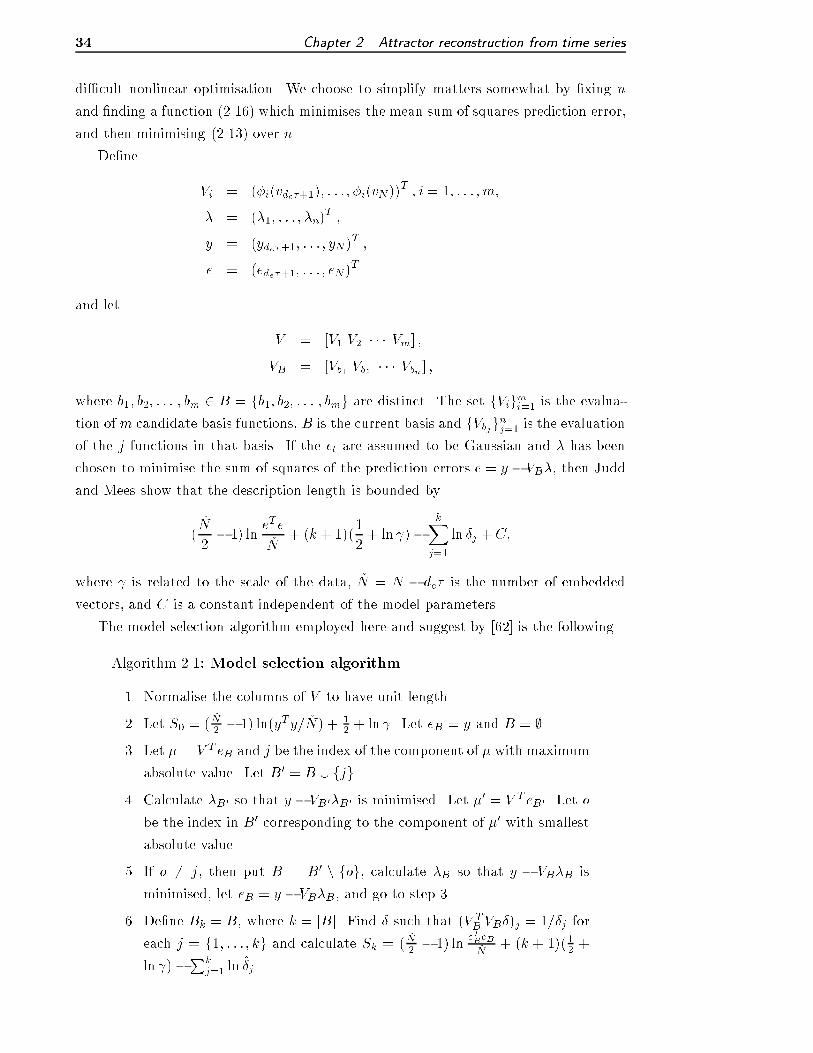
34 Chapter 2. Attractor reconstruction from time series
di�cult nonlinear optimisation. We choose to simplify matters somewhat by �xing n
and �nding a function (2.16) which minimises the mean sum of squares prediction error,
and then minimising (2.13) over n.
De�ne
Vi = (�i(vde�+1); : : : ; �i(vN))T ; i = 1; : : : ; m;
� = (�1; : : : ; �n)T ;
y = (yde�+1; : : : ; yN)T ;
e = (ede�+1; : : : ; eN)T
and let
V = [V1 V2 � � � Vm] ;
VB = [Vb1 Vb2 � � � Vbn ] ;
where b1; b2; : : : ; bm 2 B = fb1; b2; : : : ; bmg are distinct. The set fVigmi=1 is the evalua-
tion of m candidate basis functions, B is the current basis and fVbjgnj=1 is the evaluation
of the j functions in that basis. If the �t are assumed to be Gaussian and � has been
chosen to minimise the sum of squares of the prediction errors e = y � VB�, then Judd
and Mees show that the description length is bounded by
(�N
2� 1) ln
eTe�N
+ (k + 1)(1
2+ ln )�
kXj=1
ln �j + C;
where is related to the scale of the data, �N = N � de� is the number of embedded
vectors, and C is a constant independent of the model parameters.
The model selection algorithm employed here and suggest by [62] is the following.
Algorithm 2.1: Model selection algorithm.
1. Normalise the columns of V to have unit length.
2. Let S0 = (�N2 � 1) ln(yTy= �N) + 1
2 + ln . Let eB = y and B = ;.
3. Let � = V T eB and j be the index of the component of � with maximum
absolute value. Let B0 = B [ fjg.
4. Calculate �B0 so that y � VB0�B0 is minimised. Let �0 = V T eB0. Let o
be the index in B0 corresponding to the component of �0 with smallest
absolute value.
5. If o 6= j, then put B = B0 n fog, calculate �B so that y � VB�B is
minimised, let eB = y � VB�B, and go to step 3.
6. De�ne Bk = B, where k = jBj. Find � such that (V TB VB�)j = 1=�j for
each j = f1; : : : ; kg and calculate Sk = (�N2 � 1) ln
eTBeB�N
+ (k + 1)(12 +
ln )�Pk
j=1 ln �̂j .

2.3. Radial basis modelling 35
7. If some stopping condition has not been meet, then go to step 3.
8. Take the basis Bk such that Sk is minimum as the optimal model.
Note that the �j that satisfy (2.12) are calculated at step 6. Typically one will con-
tinue increasing k until it is clear that the minimum of Sk has been reached. Depending
on the modelling situation the stopping condition may be k = m (in the case of reduced
autoregressive models, discussed in chapter 9), or Sk+` > Sk for 1 � ` � L (for the
general nonlinear modelling problem of this chapter and chapter 6).

36 Chapter 2. Attractor reconstruction from time series

37CHAPTER 3
The method of surrogate data
Nonlinear measures such as correlation dimension, Lyapunov exponents, and nonlinear
prediction error are often applied to time series with the intention of identifying the
presence of nonlinear, possibly chaotic behaviour (see for example [14, 120, 158] and the
references therein). Estimating these quantities and making unequivocal classi�cation
can prove di�cult and the method of surrogate data [152] is often employed to provide
some rigor and certainty. Surrogate methods proceed by comparing the value of (non-
linear) statistics for the data and the approximate distribution for various classes of
linear systems and by doing so one can test if the data have some characteristics which
are distinct from stochastic linear systems. Surrogate analysis provides a regime to test
speci�c hypotheses about the nature of the system responsible for data, nonlinear mea-
sures provide an estimate of some quantitative attribute of the system1. In this section,
we introduce some terminology and review some common methods of generating linear
surrogates.
3.1 The rationale and language of surrogate data
The general procedure of surrogate data methods has been described by Theiler and
colleagues [151, 152, 153, 154] and Takens [149]. The principle of surrogate data is the
following. One �rst assumes that the data come from some speci�c class of dynamical
process, possibly �tting a parametric model to the data. One then generates surrogate
data from this hypothetical process and calculates various statistics of the surrogates
and original data. The surrogate data will give the expected distribution of statistic
values and one can check that the original data have a typical value. If the original data
have atypical statistics, then we reject the hypothesis that the process that generated the
original data are of the assumed class. One always progresses from simple and speci�c
assumptions to broader and more sophisticated models if the data are inconsistent with
the surrogate data.
Let � be a speci�c hypothesis and F� the set of all processes (or systems) consistent
with that hypothesis. Let z 2 RN be a time series (consisting ofN scalar measurements)
under consideration, and let T : RN ! U be a statistic which we will use to test the
hypothesis � that z was generated by some process F 2 F�. Surrogate data sets zi, i =
1; 2; : : : are generated from z (and are the same length as z) and are consistent with the
hypothesis � being tested. Generally U will be in R and one can discriminate between
the data z and surrogates zi consistent with the hypothesis given the approximate
probability density pT;F (t) = Prob(T (zi) < t), i.e. the probability density of T given F .
In a recent paper, Theiler [153] suggests that there are two fundamentally di�erent
types of test statistics: pivotal; and non-pivotal.
1Because nonlinear measures are of particular interest they are often used as the discriminating
statistic in surrogate data hypothesis testing

38 Chapter 3. The method of surrogate data
De�nition 3.1:A test statistic T is pivotal if the probability density pT;F is
the same for all processes F consistent with the hypotheses; otherwise it is
non-pivotal.
Similarly there are two di�erent types of hypotheses: simple hypotheses and composite
hypotheses.
De�nition 3.2: A hypothesis is simple if the set of all processes consistent
with the hypothesis F� is singleton. Otherwise the hypothesis is composite.
When one has a composite hypothesis the problem is not only to generate surrogates
consistent with F (a particular process) but also to estimate F 2 F�. Theiler argues
that it is highly desirable to use a pivotal test statistic if the hypothesis is composite.
In the case when the hypothesis is composite, one must specify F | unless the test
statistic T is pivotal, in which case pT;F is the same for all F 2 F�. In cases when
non-pivotal statistics are to be applied to composite hypotheses (as most interesting
hypotheses are), Theiler suggests that a constrained realisation scheme be employed.
De�nition 3.3: Let F̂ 2 F� be the process estimated from the data z, and
let zi be a surrogate data set generated from Fi 2 F�. Let F̂i 2 F� be the
process estimated from zi, then a surrogate zi is a constrained realisation if
F̂i = F̂ . Otherwise it is non-constrained.
That is, as well as generating surrogates that are typical realisations of a model of the
data, one should ensure that the surrogates are realisations of a process that gives iden-
tical estimates of the parameters (of that process) to the estimates of those parameters
from the data.
For example, let � be the hypothesis that z is generated by linearly �ltered i.i.d. (in-
dependently and identically distributed) noise. Surrogates for z could be generated by
estimating (or even guessing) the best linear model (from z) and generating realisations
from this assumed model. These surrogates would be non-constrained. Constrained
realisation surrogates can be generated by shu�ing the phases of the Fourier transform
of the data (this produces a random data set with the same power spectra, and hence
autocorrelation as the data). Autocorrelation, nonlinear prediction error, or rank dis-
tribution statistics (standard deviation or higher moments) would be non-pivotal test
statistics. The probability distribution of statistic values would depend on the form of
the noise source and type of linear �lter. However, correlation dimension or Lyapunov
exponents would be pivotal test statistics, the problem is to be able to produce a pivotal
estimate of these quantities. The probability distribution of these quantities will be the
same for all processes so exactly what estimate one makes of the linear model and i.i.d.
noise source is not important. For a more complete discussion see Theiler [153].
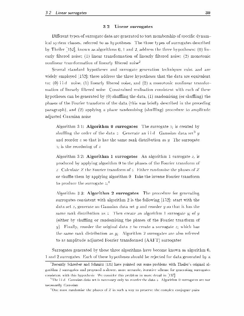
3.2. Linear surrogates 39
3.2 Linear surrogates
Di�erent types of surrogate data are generated to test membership of speci�c dynam-
ical system classes, referred to as hypotheses. The three types of surrogates described
by Theiler [152], known as algorithms 0, 1 and 2, address the three hypotheses: (0) lin-
early �ltered noise; (1) linear transformation of linearly �ltered noise; (2) monotonic
nonlinear transformation of linearly �ltered noise2.
Several standard hypotheses and surrogate generation techniques exist and are
widely employed [152]; these address the three hypotheses that the data are equivalent
to: (0) i.i.d. noise, (1) linearly �ltered noise, and (2) a monotonic nonlinear transfor-
mation of linearly �ltered noise. Constrained realisation consistent with each of these
hypotheses can be generated by (0) shu�ing the data, (1) randomising (or shu�ing) the
phases of the Fourier transform of the data (this was brie y described in the preceding
paragraph), and (2) applying a phase randomising (shu�ing) procedure to amplitude
adjusted Gaussian noise.
Algorithm 3.1: Algorithm 0 surrogates. The surrogate zi is created by
shu�ing the order of the data z. Generate an i.i.d. Gaussian data set3 y
and reorder z so that is has the same rank distribution as y. The surrogate
zi is the reordering of z.
Algorithm 3.2: Algorithm 1 surrogates. An algorithm 1 surrogate zi is
produced by applying algorithm 0 to the phases of the Fourier transform of
z. Calculate Z the Fourier transform of z. Either randomise the phases of Z
or shu�e them by applying algorithm 0. Take the inverse Fourier transform
to produce the surrogate zi4.
Algorithm 3.3: Algorithm 2 surrogates. The procedure for generating
surrogates consistent with algorithm 2 is the following [152]: start with the
data set z, generate an Gaussian data set y and reorder y so that it has the
same rank distribution as z. Then create an algorithm 1 surrogate yi of y
(either by shu�ing or randomising the phases of the Fourier transform of
y). Finally, reorder the original data z to create a surrogate zi which has
the same rank distribution as yi. Algorithm 2 surrogates are also referred
to as amplitude adjusted Fourier transformed (AAFT) surrogates.
Surrogates generated by these three algorithms have become known as algorithm 0,
1 and 2 surrogates. Each of these hypotheses should be rejected for data generated by a
2Recently Schreiber and Schmitz [121] have pointed out some problems with Theiler's original al-
gorithm 2 surrogates and proposed a slower, more accurate, iterative scheme for generating surrogates
consistent with this hypothesis. We consider this problem in more detail in [137].3The i.i.d. Gaussian data set is necessary only to reorder the data z. Algorithm 0 surrogates are not
necessarily Gaussian.4One must randomise the phases of Z in such a way to preserve the complex conjugate pairs.

40 Chapter 3. The method of surrogate data
0 100 200 300 400 500 600 700 800 900 1000
−2
0
2
(c)
0 100 200 300 400 500 600 700 800 900 1000
−2
0
2
(b)
0 100 200 300 400 500 600 700 800 900 1000
−2
0
2
(a)
Figure 3.1: Generation of cycle shu�ed surrogates: An illustration of the method
by which cycle shu�ed surrogates are generated. Plot (a) shows a section of data, split
at the peaks into its individual cycles. The second plot shows these cycles shu�ed, note
the discontinuity in plot (b). Plot (c) has a vertical shift on the individual cycles to
remove the discontinuity in (b) | this has be replaced by non-stationarity.
nonlinear system. However, rejecting these hypotheses does not necessarily indicate the
presence of a nonlinear system, only that it is unlikely that the data are generated by
a monotonic nonlinear transformation of linearly �ltered noise. The system could, for
example, involve a non-monotonic transformation or non Gaussian or state dependent
noise.
3.3 Cycle shu�ed surrogates
In the case of a periodic signal it would be useful to be able to determine the presence
of temporal correlation between cycles. In recent papers Theiler [151] (and also Theiler
and Rapp [154]) address this problem and propose that a logical choice of surrogate
for strongly periodic data, such as epileptic electroencephalogram signals, should also
be periodic. To achieve this Theiler decomposes the signal into cycles, and shu�es

3.3. Cycle shu�ed surrogates 41
the individual cycles. In a statistical framework the \block bootstrap" is proposed by
K�unsch [73]. K�unsch's algorithm decomposes and shu�es \blocks" of a data set.
Theiler's hypothesis for strongly periodic signals is rather simple, but in many ways
powerful. Theiler proposes that surrogates generated by shu�ing the cycles addresses
the hypothesis that there is no dynamical correlation between cycles.
Algorithm 3.4: Cycle shu�ed surrogates. Split the signal z into its
individual cycles (identify the location of the peak, or some other convenient
point within each cycle). Randomly reorder the cycles and form a new time
series zi by concatenating the individual cycles. If the original time series z is
even slightly non-stationary then then individual cycles will almost certainly
have to be shifted vertically to preserve the \continuity" of the original time
series z. See �gure 3.1.
In some respect this algorithm is analogous to algorithm 0, except that it tests
temporal correlation between cycles, not data points. We have examined the correlation
between cycles directly, by reducing each cycle to a single measurement [133, 139] (this
is covered in some detail in chapter 9). It is then possible not only to test algorithm 0
type hypotheses but also algorithm 1 and 2. However, reducing each cycle to a single
measurement can result in substantial loss of information. Furthermore this technique
addresses a slightly di�erent hypothesis, for this reason we do not consider such a
procedure in this review.

42 Chapter 3. The method of surrogate data

43
Part III
Analysis of infant respiration


45CHAPTER 4
Surrogate analysis
In the last two chapters we reviewed state space reconstruction methods and surrogate
data techniques common in the scienti�c literature. We intend to apply these techniques
to reconstruct the dynamics of the human infant respiratory system and determine the
nature of nonlinear behaviour present.
Chapter 5 discusses some issues concerning the estimation of embedding parameters
de and � to produce optimal reconstruction of the original dynamical system. Chapter 6
will discuss the modelling of this reconstructed system and present some new results and
modelling techniques that will allow us to build accurate nonlinear models of the dy-
namics of this system. However, to determine if noise driven simulations of these models
are su�ciently similar to the data we apply surrogate data techniques and utilise these
model simulations as nonlinear surrogates. Hence, in this section we extend current sur-
rogate data techniques to the regime of nonlinear hypothesis testing. We suggest some
conditions on the models and test statistics which will allow the application of surrogate
data techniques using non-constrained surrogates (produced as model simulations) and
we examine a pivotal test statistic based on the correlation integral.
4.1 On surrogate analysis
Surrogate analysis enables us to test whether the dynamics are consistent with lin-
early �ltered noise or a nonlinear dynamical system. We wish to apply the techniques
of surrogate analysis to infant respiratory data using correlation dimension as a dis-
criminatory test statistic1. We expect to reject the simple linear hypotheses and later
attempt to generate an acceptable nonlinear null hypothesis. Surrogate data analysis
is not, however, entirely straightforward. Theiler's original work on surrogate methods
[152] (see chapter 3), suggested a \hierarchy" of hypotheses that should be tested with
a \battery" of test statistics. More recent work [151, 154] has demonstrated that not all
test statistics are equally good. Furthermore, not all hypotheses are as straightforward,
or interesting, as they may appear. It is possible that one of the surrogate generat-
ing algorithms is awed [121] and the choice of test statistic and surrogate generation
algorithm should be made very carefully [153].
Existing surrogate methods are largely non-parametric and concerned with reject-
ing the hypothesis that a given data set is generated by some form of linear system.
We suggest a new type of surrogate generation method which is both parametric and
nonlinear. In general we are unable to identify a given time series as either chaotic or
simply nonlinear. Instead we address the simpler set of hypotheses that the data are
consistent with a noise driven nonlinear system of a particular form. We model the
data using methods described in chapters 2 and 6 (see also [62, 135]) and generate noise
driven simulations from that model. Using correlation dimension (or another nonlinear
1We present this analysis in chapter 8.

46 Chapter 4. Surrogate analysis
statistic) we are then able determine which properties are common to both data and
model.
In this section we cover some preliminary issues concerning surrogate data. We
discuss the suitability of various test statistics, some issues speci�c to algorithm 2 sur-
rogates, and a generalisation to nonlinear hypothesis testing. The remainder of this
chapter is concerned with the \pivotalness" of nonlinear measures based on the correla-
tion integral. The \pivotalness" of nonlinear measures is a vital issue to the application
of nonlinear surrogate data for hypothesis testing.
4.1.1 Test statistics To compare the data to surrogates a suitable test statistic
must be selected. To be e�ective for hypothesis testing a test statistic must be able to be
estimated reliably (it must be estimated consistently) and provide good discriminatory
power. If a test statistic provides, in its own right, useful information about the data
then this is a further bene�t of a wise choice of test statistic. Such a statistic must
measure a nontrivial invariant of a dynamical system that is independent of the way
surrogates are generated.
It is necessary that a test statistic not be invariant with respect to a given hypotheses.
That is, we do not want that for every data set z and every realisation zi of any Fi 2 F�
that T (z) = T (zi). The test statistic must measure something which is independent of
the surrogate generation method.
Unfortunately not all interesting test statistics are pivotal and constrained real-
isation schemes can be extremely nontrivial2. Furthermore, the nonlinear surrogate
generation method we propose in section 4.1.3 is a parametric modelling method that
utilises a stochastic search algorithm | it is de�nitely not a constrained realisation
method, and no related constrained method seems evident3.
In this section we brie y discuss our test statistic. We have chosen to use correlation
dimension because it is a measure of great signi�cance and has been the subject of much
attention. Neither of these qualities will ensure that correlation dimension is a good
test statistic for hypothesis testing. However, we will proceed to show that correlation
dimension can be estimated consistently and o�ers good discriminatory power as a test
statistic for hypothesis testing.
Correlation dimension, as we have de�ned it in section 2.2, is a function of "0 (see
�gure 8.7 and 8.8 for examples of correlation dimension curves). There are several
obvious ways to compare these curves. On many occasions, however, it is su�cient to
compare the value of dimension for some �xed values of "0, and this is the method we
2Theiler [153] gives examples of constrained realisation schemes for linear hypotheses, namely algo-
rithm 0, 1 and 2.3We have found it exceedingly di�cult to produce consistent estimates of parameters of a model of
a single data set (this is the subject of chapter 6). Given that we are not guaranteed the estimates of
these parameters are the same with each iteration of our modelling algorithm it is unlikely that one can
construct a constrained realisation algorithm based on these modelling methods.

4.1. On surrogate analysis 47
use. Other possibilities include the mean value of the dimension estimate, or the slope
of the line of best �t. More sophisticated methods are statistical tests such as the �2 test
or the Kolmogorov-Smirnov statistic applied to the distribution of inter-point distances
to determine if the distributions are the same.
The Kolmogorov-Smirnov test The distribution of inter-point distances CN(") (2.4)
is the probability that two points vi, vj on the attractor are less than a distance "
apart. For two distributions of inter-point distances CN("), and ~CN(") the Kolmogorov-
Smirnov test measures the maximum absolute di�erence between the distributions
max"jCN(")� ~CN(")j:
The �2 test The �2 test is a measure of the di�erence between an observed distri-
bution ~CN(") and the expected distribution CN("). The �2 test assumes some discrete
distribution and compares the expected distribution to a set of experimental obser-
vations. The correlation dimension algorithm we employ imposes a binning on the
distribution CN("). Let pi denote the expect probability of a random inter-point dis-
tance falling in the ith bin (calculated from CN(")), let Ni denote the number of inter
point distances in the ith bin (from ~CN (")), and let n denote the number of inter-point
distances. Then the �2 statistic is given by
Xi
(Ni � npi)2
npi:
Details of these tests can be found in most introductory statistics texts, see for example
[8].
Noise dimension An alternative to comparing correlation dimension curves in terms
of the distribution of inter-point distances is to extract some important (scalar) statistic
from dc("0). One such statistic is the noise dimension. The expected value of dc at scale
"0 is given by [61]
d̂c � dn � dndn + 2
"20
where dn is the noise dimension. By taking a Taylor series approximation one gets that
d̂c � (dn � dndn + 2
)� 2dn
dn + 2log "20:
Using this expression one can �t a line d̂c � m log "20 + b to the correlation dimension
curve to estimate dn � �2 mm+2 .
4.1.2 AAFT surrogates revisited Schreiber and Schmitz [121] have recently
raised concerns about aspects of algorithm 2 surrogates. Although z and zi have (by
construction) identical probability distributions they will not, in general, have identi-
cal Fourier spectra (and therefore autocorrelation). To overcome this they propose an
iterative version of the AAFT algorithm. Convergence to the same Fourier spectra is

48 Chapter 4. Surrogate analysis
not guaranteed under this method either, but their results seem to indicate a closer
agreement between power spectra. Using standard AAFT surrogate generation tech-
niques we have found that although estimates of the power spectra (through whichever
numerical scheme one chooses) may not agree very closely, autocorrelation �(�) does |
at least for small to moderately large values of � .
Recently, further concerns have also been raised over the application of algorithm
2 surrogates for almost periodic data [145] (data with a strong periodic component).
However, numerical experiments with the data used in this thesis [134, 137] demonstrate
that the di�erence between the probability distributions estimated with the algorithm
2 technique and more technical methods [121, 145] is minimal.
4.1.3 Generalised nonlinear null hypotheses Hypothesis testing with surro-
gate data is, essentially a modelling process. To test if the data are consistent with a
particular hypothesis one �rst builds a model that is consistent with that hypothesis
and has the same properties as the original data, then one generates surrogate data
from the model and checks that the original data are typical under the hypothesis by
comparing it to the surrogate data. For surrogates generated by algorithm 0, 1 or 2 the
model used is linear. Each of these surrogate tests addresses a hypothesis that the data
are either linear, or some (linear, or monotonic nonlinear) transformation of a linear
process. Although nonlinear, the hypothesis addressed by shu�ing cycles is that there
is no long term temporal structure.
To address the hypothesis that the data come from a noise driven nonlinear system,
we build a nonlinear model and generate surrogate data (noise driven simulations). The
nonlinear model that we build from the data is a cylindrical basis model by the methods
of [62, 135] (see chapters 2 and 6). Cylindrical basis models are a generalisation of radial
basis models that allow for a variable embedding [64]. Cylindrical basis models are used
because they are known to be e�ective in modelling a variety of nonlinear dynamical
systems and the author has at his disposal a sophisticated software implementation of
this modelling method. The hypothesis we wish to test is that the data are consistent
with a nonlinear system that can be described by a cylindrical basis model and that the
data of such a system can be modelled adequately using the algorithms we use. Rejection
of the hypothesis could imply that the data cannot be described by a cylindrical basis
model, or that the modelling algorithm failed to build an accurate model. We return to
discuss this hypothesis in section 4.1.1.
Building a nonlinear model of data is a decidedly nontrivial process. In section 2.3 we
introduced the general form (2.16) of these models and we discussed some detail of the
modelling algorithm. Chapter 6 suggests some re�nement to this modelling algorithm
to produce improved results.
The conclusions that can be drawn from testing with these nonlinear models are
several. Surrogate data hypothesis testing can indicate that our data are not consistent

4.1. On surrogate analysis 49
with a nonlinear system of the type generated by our modelling procedure. Furthermore,
this is a test of the modelling procedure itself. If the hypothesis cannot be rejected on
the basis of our analysis then this will indicate that the model we have built is an
accurate model of the data, with respect to correlation dimension. Failure to reject
the null hypothesis can indicate successful and accurate modelling of the data. Even if
correlation dimension cannot distinguish between data and surrogate, other measures,
for example largest Lyapunov exponent, may.
There is one important caveat. Our methods do not test for the presence of a general
nonlinear periodic orbit (for example). They only test for the presence of a nonlinear
periodic orbit that can be accurately modelled as the sum of cylindrical basis functions of
the form described in section 2.3.3. This is not particularly restrictive since experience
has shown that such functions can model a wide range of phenomena [62, 63, 64].
4.1.4 The \pivotalness" of dynamic measures Theiler and Prichard [153]
argue that by using algorithms that generate constrained realisations to generate surro-
gates, one is free to use almost any statistic one wishes. On the other hand if one does
not use such methods to generate surrogates, it is necessary to select a statistic which
has exactly the same distribution of statistic values for all realisations consistent with
the hypothesis being tested. When generating nonlinear surrogates, we suggest that
it may be easier to use a pivotal test statistic, and choose realisations of any process
consistent with that hypothesis as representative. With such a statistic it would be
possible to build a nonlinear model (usually with reference to the data) and generate
(noise driven) simulations from that model as surrogates.
However, with this approach it is necessary to check that the probability distribution
of the test statistic is independent of the particular model we have built, or determine
for which models the distribution is the same. We can only test a hypothesis as broad
as the set of all processes which have the same probability distribution of test statistic
values. For example, if the distribution of the test statistic is di�erent for every model
then the only hypothesis we can test is that the data are consistent with a speci�c
model. However, if all models within some class (for example, two dimensional periodic
orbits) have the same distribution of statistic values then the hypothesis which we can
test with realisations from any one of these models is much broader (for example, the
hypothesis that the system has a two dimensional periodic orbit).
Unlike Theiler's algorithm 0, 1 and 2 surrogates, when testing with nonlinear sur-
rogates (simulations of a model) the hypothesis being tested is not known a priori, but
will be determined by the \pivotalness" of the test statistic. To illustrate our approach
we choose to use correlation dimension. Other statistics, particularly measures derived
from dynamical system theory that are invariant under di�eomorphisms and can be
consistently estimated (i.e. any quantity one can reliably estimate from a time-delay

50 Chapter 4. Surrogate analysis
embedding4) may serve equally well. It is important to show that the statistic being
estimated can be estimated consistently. We choose to use correlation dimension as a
test statistic because we have a reliable algorithm to estimate it, that is well understood
[37, 60, 61]. Neither correlation dimension nor the algorithm we employ to estimate it
are necessarily unique in their suitability as test statistics.
For hypotheses such as those addressed by nonlinear models one must determine the
hypothesis for which the test is pivotal. If F� is the set of all noise driven processes then
dc(") will not be pivotal. However, if we restrict ourselves to F~� � F� where T is pivotal
on F~� then the problem is resolved. To do this we simply rephrase the hypothesis to
be that the data are generated by a noise driven nonlinear function (modelled by a
cylindrical basis model) of dimension d. For example this allows us to test if the data
are generated by a periodic orbit with 2 degrees of freedom driven by Gaussian noise.
The rest of this chapter will be concerned with presenting some new theoretical
and experimental results concerning the application of correlation dimension as a test
statistic for speci�c (linear and nonlinear) hypotheses. This is largely based on orig-
inal work published in [137], [134, 143] provide reviews of some of these techniques.
We show that correlation dimension is a useful test statistic for linear surrogates gen-
erated by traditional [152] or more naive (parametric) methods, as well as nonlinear
surrogates generated as noise driven simulations of nonlinear parametric models. We
demonstrate the application of correlation dimension as a test statistic for nonlinear
hypothesis testing with speci�c experimental data sets. In sections 4.2 and 4.3 we dis-
cuss new results concerning the \pivotalness" of correlation dimension for linear and
nonlinear surrogates. In chapter 8 we demonstrate the application of these methods
with some experimental data collected from sleeping infants.
4.2 Correlation dimension as a pivotal test statistic | linear hypotheses
The linear processes consistent with the hypotheses addressed by algorithm 0, 1 and
2 are all forms of �ltered noise, and hence in�nite dimensional. That is, the correlation
dimension will be in�nite. We will argue that a dimension estimation algorithm which
relies on a time delay embedding will (or should) produce the same probability density
of estimates of correlation dimension for any data set consistent with one of these
hypotheses. To do this in general we could invoke Takens' embedding theorem [148].
Takens' theorem ensures that a time delay embedding scheme will produce faithful
reconstruction of an attractor (provided de > 2dc + 1) if the measurement function is
C2. When dc is �nite, one simply needs a su�ciently large value of de. In the case when
dc is in�nite, Takens' theorem no longer applies. However if dc is in�nite (or indeed if
dc > de) the embedded time series will \�ll" the embedding space. If the time series is of
in�nite length then the dimension dc of the embedded time series will then be equal to
de. If the time series is �nite then the dimension dc of the embedded time series will be
4In particular statistics based on the correlation integral.

4.2. Correlation dimension as a pivotal test statistic | linear hypotheses 51
less than de5. For a moderately small embedding dimension this di�erence is typically
not great and is dependent on the estimation algorithm and the length of the time series,
and independent of the particular realisation. Hence, if the correlation dimension dc
of all surrogates consistent with the hypothesis under consideration exceeds de then
correlation dimension is a pivotal test statistic for that value of de.
An examination of the \pivotalness" of the correlation integral (and therefore cor-
relation dimension) can be found in a recent paper of Takens [149]. Takens' approach
is to observe that, if � and �0 are two distance functions in the embedded space X (we
consider X = Rn, Takens considers a general compact q-dimensional manifold) and k
is some constant and for all x; y 2 X
k�1�(x; y) � �0(x; y) � k�(x; y) (4.1)
then the correlation integral limN!1 CN(") with respect to either distance function
is similarly bounded and hence the correlation dimension with respect to each metric
will be the same. This result is independent of the conditions of Takens' embedding
theorem (i.e. that n > 2dc + 1 for X = Rn). Hence if we (for example) embed a
stochastic signal in Rn the correlation dimension will have the same value with respect
to the two di�erent distance functions � and �0. To show that dc is pivotal for the various
linear hypotheses addressed by algorithm 0, 1 and 2 it is only necessary to show that
various transformations can be applied to a realisation of such processes which have the
a�ect of producing i.i.d. noise and are equivalent to a bounded change of metric as in
(4.1).
Our approach is to show that surrogates consistent with each of the three standard
linear hypotheses are at most a C2 function from Gaussian noise N(0; 1). A C2 function
on a bounded set (a bounded attractor or a �nite time series) distorts distance only by
a bounded factor (as in equation (4.1)) and so the correlation dimension is invariant.
We therefore have the following new result.
Proposition 4.1: The correlation dimension dc is a pivotal test statistic
for a hypothesis � if 8F1; F2 2 F� and embeddings �1;2 : R 7�! X1;2 there
exists an invertible C2 function f : X1 7�! X2 such that 8 t f(�1(F1(t))) =�2(F2(t)).
Proof: The proof of this proposition is outlined in the proceeding argu-
ments. Let F1; F2 2 F� be particular processes consistent with a given
hypothesis and F1(t) and F2(t) realisations of those processes. We have that
8tf(�1(F1(t))) = �2(F2(t)), and so if �1(x1); �1(y1) 2 X1 and �2(x2); �2(y2) 2X2 are points on the embeddings �1 and �2 of F1(t) and F2(t) respectively,
then f(�1(x1)) = �2(x2) and f(�1(y1)) = �2(y2). Let �2 be a distance
5This is particularly likely for a short time series and large embedding dimension.
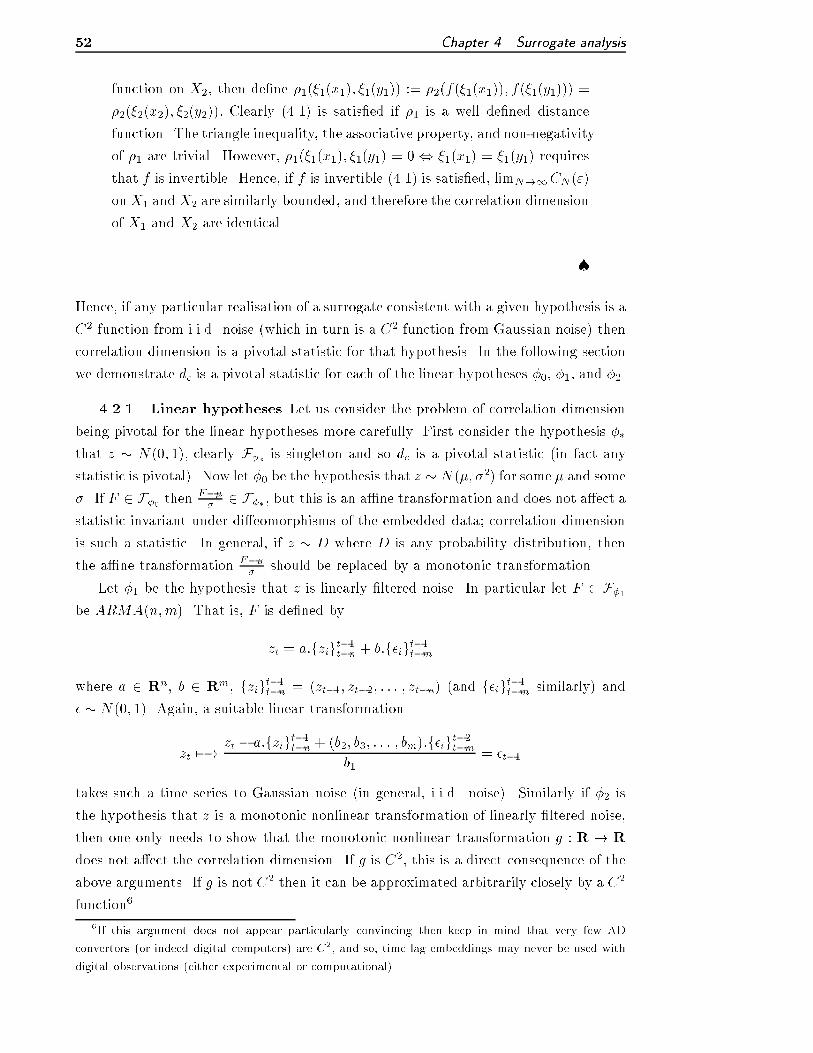
52 Chapter 4. Surrogate analysis
function on X2, then de�ne �1(�1(x1); �1(y1)) := �2(f(�1(x1)); f(�1(y1))) =
�2(�2(x2); �2(y2)): Clearly (4.1) is satis�ed if �1 is a well de�ned distance
function. The triangle inequality, the associative property, and non-negativity
of �1 are trivial. However, �1(�1(x1); �1(y1) = 0 , �1(x1) = �1(y1) requires
that f is invertible. Hence, if f is invertible (4.1) is satis�ed, limN!1CN(")
onX1 and X2 are similarly bounded, and therefore the correlation dimension
of X1 and X2 are identical.
�
Hence, if any particular realisation of a surrogate consistent with a given hypothesis is a
C2 function from i.i.d. noise (which in turn is a C2 function from Gaussian noise) then
correlation dimension is a pivotal statistic for that hypothesis. In the following section
we demonstrate dc is a pivotal statistic for each of the linear hypotheses �0, �1, and �2.
4.2.1 Linear hypotheses Let us consider the problem of correlation dimension
being pivotal for the linear hypotheses more carefully. First consider the hypothesis ��that z � N(0; 1), clearly F�� is singleton and so dc is a pivotal statistic (in fact any
statistic is pivotal). Now let �0 be the hypothesis that z � N(�; �2) for some � and some
�. If F 2 F�0 thenF��� 2 F�� , but this is an a�ne transformation and does not a�ect a
statistic invariant under di�eomorphisms of the embedded data; correlation dimension
is such a statistic. In general, if z � D where D is any probability distribution, then
the a�ne transformation F��� should be replaced by a monotonic transformation.
Let �1 be the hypothesis that z is linearly �ltered noise. In particular let F 2 F�1
be ARMA(n;m). That is, F is de�ned by
zt = a:fzigt�1t�n + b:f�igt�1t�m
where a 2 Rn, b 2 Rm, fzigt�1t�n = (zt�1; zt�2; : : : ; zt�n) (and f�igt�1t�m similarly) and
� � N(0; 1). Again, a suitable linear transformation
zt 7�!zt � a:fzigt�1t�n + (b2; b3; : : : ; bm):f�igt�2t�m
b1= �t�1
takes such a time series to Gaussian noise (in general, i.i.d. noise). Similarly if �2 is
the hypothesis that z is a monotonic nonlinear transformation of linearly �ltered noise,
then one only needs to show that the monotonic nonlinear transformation g : R ! R
does not a�ect the correlation dimension. If g is C2, this is a direct consequence of the
above arguments. If g is not C2 then it can be approximated arbitrarily closely by a C2
function6.
6If this argument does not appear particularly convincing then keep in mind that very few AD
convertors (or indeed digital computers) are C2, and so, time lag embeddings may never be used with
digital observations (either experimental or computational).

4.2. Correlation dimension as a pivotal test statistic | linear hypotheses 53
The above arguments do not guarantee that the correlation dimension dc("0) esti-
mated by Judd's algorithm will be a pivotal statistic, it only implies that the actual
correlation dimension will be. The technical details of Judd's algorithm have been con-
sidered elsewhere [60, 61], and an independent evaluation of this algorithm is given by
Galka and colleagues [37]. Provided one chooses a suitably small scale "0 the statistic
dc("0) will be (asymptotically) pivotal. The above argument, in conjunction with tech-
nical results concerning Judd's algorithm [37, 60, 61], imply that correlation dimension
estimated by this algorithm is pivotal and the estimates are consistent.
4.2.2 Calculations Estimates of the probability density of correlation dimension
for various linear surrogates are shown in �gures 4.1, 4.2 and 4.4. Figures 4.1 and 4.2
compare the estimates of pT;F (t) for various classes of simple and composite hypotheses
concerned with algorithm 1 (�gure 4.1) and 2 (�gure 4.2). Figure 4.4 compares di�erent
constrained and non-constrained realisation techniques for the experimental data of
�gure 4.3. In each case the probability density of correlation dimension pdc("0);F (t)
was estimated for �xed values of "0 by linearly interpolating the individual correlation
dimension estimates to get an ensemble of values of dc("0) from which pdc("0);F (t) is
estimated following methods described by [127]. The ensemble of probability density
estimates were then used to calculate the contour plots of pdc("0);F (t) for all values of "0
for which our correlation dimension estimation algorithms converged.
Figures 4.1 and 4.2 show that the probability density of correlation dimension is
independent of which particular form of linear �ltering one applies. In both �gure 4.1
and �gure 4.2, the �rst panel shows an estimate of the probability density function
(p.d.f.) of correlation dimension for realisations given a particular (in �gure 4.2, mono-
tonic nonlinearly �ltered) autoregressive process; the second panel shows an estimate
of the p.d.f. from surrogates of one of the realisations in the �rst panel. The third and
fourth panels show estimates of the p.d.f. of correlation dimension for realisations of
di�erent (stable) autoregressive processes.
The probability density plot for AAFT (algorithm 2) surrogates is virtually iden-
tical to that for di�erent realisations of a single process, and for random processes.
This agreement is particularly strong between the �rst two panels of each �gure (dis-
tinct realisations of one process and surrogates of a single realisation). The slightly
greater variation with the third and fourth panels is most probably a result of the scal-
ing properties of our estimates of correlation dimension. However, this only produces
convergence of the correlation dimension estimates at di�erent scales "0, not distinct
probability distributions. The plots only fail to agree for values of "0 for which an es-
timate of dc("0) was not obtained. The panels in �gure 4.1 show precise agreement for
the range �2 <� log("0) <� �1:8, in �gure 4.2 the range is �5 <� log("0) <� �3:7. Outsidethese ranges one or more of the panels correspond to surrogates that failed to produce
convergence of the correlation dimension algorithm at that particular scale.

54 Chapter 4. Surrogate analysis
−2.4 −2.2 −2 −1.8
4
4.5
5
log(epsilon0)
corr
elat
ion
dim
ensi
on(i)
−2.4 −2.2 −2 −1.8
4
4.5
5
log(epsilon0)
corr
elat
ion
dim
ensi
on
(ii)
−2.4 −2.2 −2 −1.8
4
4.5
5
log(epsilon0)
corr
elat
ion
dim
ensi
on
(iii)
−2.4 −2.2 −2 −1.8
4
4.5
5
log(epsilon0)
corr
elat
ion
dim
ensi
on
(iv)
Figure 4.1: Probability distribution for correlation dimension estimates of
AR(2) processes: Shown are contour plots which represent the probability density
of correlation dimension estimate for various values of "0. Figure (i) is the probability
distribution function (p.d.f.) for various realisations of the AR(2) process xn�0:4xn�1+0:7xn�2 = �n, �n � N(0; 1), �gure (ii) shows the p.d.f. for AAFT surrogates of one of
these processes. Figure (iii) and (iv) are for random (stable) AR(2) processes. In each
of these two calculations �1 and �2 were selected uniformly (subject to j�1j; j�2j < 1)
and the autoregressive process is xn+(�1+�2)xn�1+�1�2xn�2 = �n, �n � N(0; 1) (see
[104]). In the third plot �1; �2 2 R, in the fourth �1; �2 2 C. For each calculation 50
realisations of 4000 points were calculated, and their correlation dimension calculated for
embedding dimension de = 3; 4; 5; 10; 15 (shown are the results for de = 5) using a 10000
bin histogram to estimate the density of inter-point distances, the other calculations
produced similar results. Note, for some values of "0 (particularly in (iii)) our dimension
estimation algorithm did not provide a value for dc("0). This does not indicate that
the estimate of the probability density of correlation dimension are distinct, only that
we were unable to estimate correlation dimension. In each case our calculations show a
very good agreement between the p.d.f. of dc("0) for all values of "0 for which a reliable
estimate could be obtained.

4.2. Correlation dimension as a pivotal test statistic | linear hypotheses 55
−5 −4.5 −4 −3.51.4
1.6
1.8
2
2.2
2.4
log(epsilon0)
corr
elat
ion
dim
ensi
on
(i)
−5 −4.5 −4 −3.51.4
1.6
1.8
2
2.2
2.4
log(epsilon0)
corr
elat
ion
dim
ensi
on
(ii)
−5 −4.5 −4 −3.51.4
1.6
1.8
2
2.2
2.4
log(epsilon0)
corr
elat
ion
dim
ensi
on
(iii)
−5 −4.5 −4 −3.51.4
1.6
1.8
2
2.2
2.4
log(epsilon0)
corr
elat
ion
dim
ensi
on
(iv)
Figure 4.2: Probability density for correlation dimension estimates of a mono-
tonic nonlinear transformation of AR(2) processes: Shown are contour plots
which represent the probability density of correlation dimension estimate for various
values of "0. Similar to �gure 4.1, the four plots are of the p.d.f. of dc("0) for: (i) var-
ious realisations of the AR(2) process xn � 0:4xn�1 + 0:7xn�2 = �n, �n � N(0; 1),
observed by g(x) = x3; (ii) AAFT surrogates of one of these processes; (iii) ran-
dom (stable) AR(2) processes observed by g(x) = x3; (iv) random (stable, pseudo-
periodic) AR(2) process observed by g(x) = x3. For these last two calculations �1 and
�2 were selected uniformly (subject to j�1j; j�2j < 1) and the autoregressive process
is xn + (�1 + �2)xn�1 + �1�2xn�2 = �n, �n � N(0; 1). In (iii) �1; �2 2 R, in (iv)
�1; �2 2 C. In each calculation 50 realisations of 4000 points were calculated, and their
correlation dimension calculated for de = 3; 4; 5; 10; 15 (shown are the results for de = 5,
the other calculations produced similar results) using a 10000 bin histogram to estimate
the distribution of inter-point distances. In each case our calculations show a very good
agreement between the p.d.f. of dc("0) for all values of "0 for which a reliable estimate
could be obtained. Similar results were also obtained using g(x) = sign(x)jxj1=4 as anobservation function.

56 Chapter 4. Surrogate analysis
0 500 1000 1500 2000 2500 3000 3500 4000−2
−1
0
1
2(a) Abdominal movement
0 500 1000 1500 2000 2500 3000 3500 4000−6
−4
−2
0
2
4(b) Electrocardiogram
Figure 4.3: Experimental data: The abdominal rib movement and electrocardiogram
signal for an 8 month old male child in rapid eye movement (REM) sleep. The 4000
data points were sampled at 50Hz, and digitised using a 12 bit analogue to digital
convertor during a sleep study at Princess Margaret Hospital for Children, Subiaco,
Western Australia. These data are from group A (section 1.2.2).
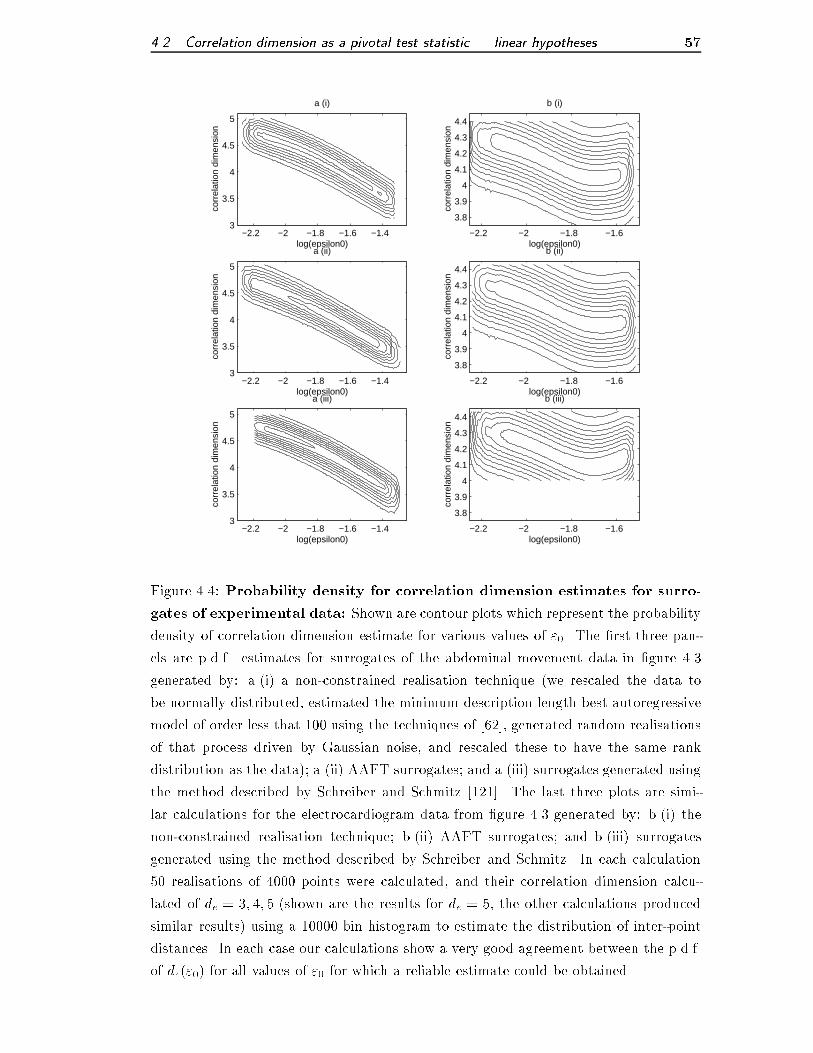
4.2. Correlation dimension as a pivotal test statistic | linear hypotheses 57
−2.2 −2 −1.8 −1.6 −1.43
3.5
4
4.5
5
log(epsilon0)
corr
elat
ion
dim
ensi
on
a (i)
−2.2 −2 −1.8 −1.6 −1.43
3.5
4
4.5
5
log(epsilon0)
corr
elat
ion
dim
ensi
on
a (ii)
−2.2 −2 −1.8 −1.6 −1.43
3.5
4
4.5
5
log(epsilon0)
corr
elat
ion
dim
ensi
on
a (iii)
−2.2 −2 −1.8 −1.6
3.8
3.9
4
4.1
4.2
4.3
4.4
log(epsilon0)
corr
elat
ion
dim
ensi
on
b (i)
−2.2 −2 −1.8 −1.6
3.8
3.9
4
4.1
4.2
4.3
4.4
log(epsilon0)
corr
elat
ion
dim
ensi
on
b (ii)
−2.2 −2 −1.8 −1.6
3.8
3.9
4
4.1
4.2
4.3
4.4
log(epsilon0)
corr
elat
ion
dim
ensi
on
b (iii)
Figure 4.4: Probability density for correlation dimension estimates for surro-
gates of experimental data: Shown are contour plots which represent the probability
density of correlation dimension estimate for various values of "0. The �rst three pan-
els are p.d.f. estimates for surrogates of the abdominal movement data in �gure 4.3
generated by: a.(i) a non-constrained realisation technique (we rescaled the data to
be normally distributed, estimated the minimum description length best autoregressive
model of order less that 100 using the techniques of [62], generated random realisations
of that process driven by Gaussian noise, and rescaled these to have the same rank
distribution as the data); a.(ii) AAFT surrogates; and a.(iii) surrogates generated using
the method described by Schreiber and Schmitz [121]. The last three plots are simi-
lar calculations for the electrocardiogram data from �gure 4.3 generated by: b.(i) the
non-constrained realisation technique; b.(ii) AAFT surrogates; and b.(iii) surrogates
generated using the method described by Schreiber and Schmitz. In each calculation
50 realisations of 4000 points were calculated, and their correlation dimension calcu-
lated of de = 3; 4; 5 (shown are the results for de = 5, the other calculations produced
similar results) using a 10000 bin histogram to estimate the distribution of inter-point
distances. In each case our calculations show a very good agreement between the p.d.f.
of dc("0) for all values of "0 for which a reliable estimate could be obtained.

58 Chapter 4. Surrogate analysis
There is substantial di�erence between the probability densities shown in �gure 4.1
and those for �gure 4.2. The di�erence results from the di�erent observation function
g(x) = x3 in �gure 4.27. This indicates a di�erence in the results of the dimension
estimation algorithm, the nonlinear transformation g has changed the scale of structure
present in the original process, and so yields di�erent values of dc("0). This indicates
that correlation dimension is not pivotal over F�2 , however, provided one can make a
reasonable estimate of the process F 2 F�2 which generated z then T is pivotal for the
restricted class F ~�2where F 2 F ~�2
� F�28. Note that the range of values of � log "0
shown in �gures 4.1 and 4.2 are quite distinct, the correlation dimension algorithm does
not produce di�erent probability density functions, it has only failed to produce an
estimate at some scales.
Figure 4.4 gives a comparison of the probability distribution for two di�erent data
sets with various di�erent surrogate generation methods. In each column the �rst panel
shows results for a non-constrained surrogate generation method (we estimated the
parameters of the best autoregressive model and generated simulations from it, see the
caption of �gure 4.4), and constrained surrogate methods suggested by Theiler (panel
ii) and Schreiber and Schmitz (panel iii). The surrogates generated by either simple
parameter estimation methods, the AAFTmethod or the method suggested by Schreiber
and Schmitz9 produced almost identical results. Hence in this example any surrogate
generation method will serve equally well, provided the surrogates are not completely
di�erent from the data. This con�rms our earlier arguments and calculations with
stochastic processes.
4.2.3 Results The close agreement between the probability density estimates in
the �rst two panels of each of �gures 4.1 and 4.2 and panels a.(i)-(iii) and b.(i)-(iii) in
�gure 4.4 indicate that the surrogate generation methods suggested by Theiler [152] and
those of Schreiber and Schmitz [121] generate surrogates for which dc("0) is pivotal. This
should be the case as these are all constrained realisation techniques (with the possible
exception of algorithm 2 surrogates [121]). The agreement between all four panels in
�gure 4.1 (and similarly between all four panels in �gure 4.2) indicate that dc("0) is
virtually pivotal when � is the hypothesis that the data are linearly �ltered noise or
a particular monotonic nonlinear transformation of linearly �ltered noise. There are
minor di�erences between the various panels in each �gure, but these are only a result
of the estimate of dc("0) not converging.
7We also repeated the calculations of �gure 4.2 with g(x) = sign(x)jxj1=4 (note that this function is
not C2) and obtained another set of similar results. All the individual probability density plots were
the same, but they were di�erent from those in �gures 4.1 and 4.2.8One would expect that the nonlinear transformation g would be fairly similar for all F 2 F ~�2
.
From our calculations it appears su�cient to ensure that the data and surrogates have identical rank
distributions.9We iterated the algorithm described in [121] 1000 times to generate each surrogate.

4.3. Correlation dimension as a pivotal test statistic | nonlinear hypothesis 59
The di�erence between the results of �gure 4.1 and those of �gure 4.2 indicate that
our estimate of correlation dimension is not pivotal for the hypotheses that the data are
any monotonic nonlinear transformation of linearly �ltered noise. The scale dependent
properties of dc("0) have altered the value of this statistic for various observation func-
tions g. The linear models built to estimate pdc("0);F produced estimates of correlation
dimension which closely agreed with those from the constrained surrogate generation
methods. This indicates that a non-constrained realisation technique can do as well as
a constrained one.
Correlation dimension estimates dc("0) are not pivotal for the set of all processes
consistent with the hypothesis that the data are a monotonic nonlinear transformation
of linearly �ltered noise (otherwise all the probability density estimate in �gures 4.1,
4.2, and 4.4 would be identical). However, the p.d.f. of dc("0) for various realisations
are similar enough to allow for the use of some more general non-constrained surrogate
generation methods (such as the parametric model estimation we employ in �gure 4.4
panel a.(i) and b.(i), and possibly the method suggested in [149]). Furthermore the
p.d.f. of dc values for the surrogate generation methods of Schreiber and Schmitz [121]
and Theiler [152] are identical.
The di�erence in the results between �gures 4.1, 4.2, and 4.4 is most likely a result
of the di�erent choice of observation function g a�ecting the scaling properties of the
correlation dimension estimate. By ensuring the rank distribution of the data and sur-
rogate are the same (as in �gure 4.4, panels a.(i) and b.(i)) one can generate surrogates
for which dc is pivotal. Alternatively one could choose a statistic without such sensitive
scale dependence. However, for nonlinear hypothesis testing the author believes that
sensitivity to scaling properties is an important feature of this particular test statistic.
4.3 Correlation dimension as a pivotal test statistic | nonlinear
hypothesis
Beyond applying these linear hypotheses one may wish to ask more speci�c questions;
are the data consistent with (for example) a noise driven periodic orbit? In particular,
a hypothesis similar to this is treated by Theiler's cycle shu�ed surrogates (section
3.3), we apply this method in sections 8.2.3 and 8.3.3. In this section we focus on more
general hypotheses. An experimental application of these methods has been presented
elsewhere and will appear latter in this thesis. In chapter 8 we test the hypothesis
that infant respiration during quiet sleep is distinct from a noise driven (or chaotic)
quasi-periodic, toroidal, or ribbon attractor (with more than two identi�able periods).
Such an apparently abstract hypothesis can have real value, these results have been
con�rmed with observations of cyclic amplitude modulation in the breathing of sleeping
infants [133, 140] (chapters 8 and 9) during quiet sleep and in the resting respiration of
adults at high altitude [160].

60 Chapter 4. Surrogate analysis
To apply such complex hypotheses we build cylindrical basis models using a min-
imum description length criterion (see section 2.3 and chapter 6) and generate noise
driven simulations (surrogate data sets) from these models. This modelling scheme
has been successful in modelling a wide variety of nonlinear phenomena. However, it
involves a stochastic search algorithm. This method of surrogate generation does not
produce surrogates that can be used with a constrained realisation scheme10, and so a
pivotal statistic is needed.
4.3.1 Nonlinear hypotheses It is important to determine if the data are gen-
erated by a process consistent with a speci�c model or a general class of models. To do
this we need to determine exactly how representative a particular model is for a given
test statistic | how big is the set F� for which T is pivotal? By comparing a data set
and surrogates generated by a speci�c model, are we just testing the hypothesis that a
process consistent with this speci�c model generated the data or can we infer a broader
class of models? In either case (unlike constrained realisation linear surrogates), it is
likely that the hypothesis being tested will be determined by the results of the mod-
elling procedure and therefore depend on the particular data set one has. Many of the
arguments of section 4.2 apply here as well; the hypothesis one can test will be as broad
as the class of all systems with distance function bounded by equation (4.1) (in the case
of correlation integral based test statistics). In particular proposition 4.1 holds | an
invertible C2 function will yield only a bounded change in the correlation integral.
Consider the other side of the problem. We want T to be a pivotal test statistic
for the hypothesis �, where � is a broad class of nonlinear dynamical processes. For
example, if F� is the set of all noise driven processes then dc("0) will not be pivotal.
However, if we are able to restrict ourselves to F~� � F� where T is pivotal on F~�
then the problem is resolved. To do this we simply rephrase the hypothesis to be that
the data are generated by a noise driven nonlinear function (modelled by a cylindrical
basis model) of dimension d. For example, this would allow one to test if the data are
consistent with a periodic orbit with 2 degrees of freedom driven by Gaussian noise.
Furthermore, the scale dependent properties of our estimate of dc("0) provide some
sensitivity to the size (relative to the size of the data) of structures of a particular
dimension. This is a much more useful hypothesis than that the process is noisy and
nonlinear | if this was our hypothesis, then what would be the alternative? Because of
the complexity of our dimension estimation algorithm and the class of nonlinear models
it is necessary to compare calculations of the probability density of the test statistic
for various models. Having done so one cannot make any general claims about the
\pivotalness" of a given statistic. However, for a given data set it is possible to compare
the probability distributions of a test statistic for various classes of nonlinear models
10If we are unable to estimate the model parameters consistently (from a single data set) then we are
certainly not going to be able to produce a surrogate which yields the same estimates of parameters as
the data.

4.3. Correlation dimension as a pivotal test statistic | nonlinear hypothesis 61
0 200 400 600 800 1000 1200 1400 1600−2
−1
0
1
2
3
4Abdominal movement
Figure 4.5: Experimental data: The abdominal rib movement for an 2 month old
female child in quiet (stage 3{4) sleep. The 1600 data points were sampled at 12.5Hz
(to ease the computational load involved in building the cylindrical basis model this
has been reduced from 50Hz), and digitised using a 12 bit analogue to digital convertor
during a sleep study at Princess Margaret Hospital for Children, Subiaco, Western
Australia. These data are from group A (section 1.2.2) and is the same data set as
illustrated in �gure 6.1.
and depending on the \pivotalness" of the statistics determine the hypothesis being
tested.
4.3.2 Calculations Figure 4.6 presents some experimental results from the data
of �gure 4.5. We have estimated the probability density for an ensemble of models and
for particular models from an experimental data set.
We employ a di�erent data set here for illustration purposes11 these data are far more
non-stationary than that in �gure 4.3, and proves to be a greater modelling challenge.
These calculations con�rm that the distribution of correlation dimension estimates for
di�erent realisation of one model are the same as for di�erent realisations of many
models. The models used in this calculation were selected to have simulations with
asymptotically stable periodic orbits. Models of this data set produce simulations with
either asymptotic stable periodic orbits or �xed points (the second behaviour is clearly
an inappropriate model of respiration). The p.d.f. of dc for all models therefore exhibits
two modes. We are only concerned with a unimodal distribution at any one time.
Figure 4.6 (ii), (iii) and (iv) show the probability density for particular models se-
lected from the ensemble of models used in (i). Panel (iii) is the result of the calculations
for the model which gave the smallest estimate of dc("0) for log("0) = 1:8 in (i), that is
11These calculations have also been repeated with the data in �gure 4.3 and equivalent conclusions
were reached.

62 Chapter 4. Surrogate analysis
−3 −2.5 −2 −1.5
1.6
1.8
2
2.2
2.4
2.6
log(epsilon0)
corr
elat
ion
dim
ensi
on(iv)
−3 −2.5 −2 −1.5
1.6
1.8
2
2.2
2.4
2.6
log(epsilon0)
corr
elat
ion
dim
ensi
on
(iii)
−3 −2.5 −2 −1.5
1.6
1.8
2
2.2
2.4
2.6
log(epsilon0)
corr
elat
ion
dim
ensi
on
(ii)
−3 −2.5 −2 −1.5
1.6
1.8
2
2.2
2.4
2.6
log(epsilon0)
corr
elat
ion
dim
ensi
on
(i)
Figure 4.6: Probability density for correlation dimension estimates for non-
linear surrogates of experimental data: Shown are contour plots which represent
the probability density of correlation dimension estimate for various values of "0. The
data used in this calculation is illustrated in �gure 4.5. The �gures are p.d.f. estimates
for surrogates generated from: (i) realisations of distinct models; (ii) realisations for one
of the models used in (i) with approximately the median value of correlation dimension
(dc("0) for log "0 = �1:8); (iii) realisations for the model used in (i) with the minimum
value of correlation dimension; (iv) realisations for the model used in (i) with the max-
imum value of correlation dimension. In each calculation 50 realisations of 4000 points
were calculated, and their correlation dimension calculated of de = 3; 4; 5 (shown are
the results for de = 5, the other calculations produced equivalent results) using a 10000
bin histogram to estimate the distribution of inter-point distances. In each case our
calculations show a very good agreement between the p.d.f. of dc("0) for all values of
"0 for which a reliable estimate could be obtained.

4.4. Conclusion 63
the model that generated the simulation with the lowest dimension. Panel (iv) is the
result of the calculations for the model which gave the highest dimension estimate in
(i). Panel (ii) corresponds to the median dimension estimate in (i). Despite this, all
these probability densities are very nearly the same; there is no low bias in (iii) and
no high bias in (iv). This indicates that dc("0) is (asymptotically) pivotal, simulations
from any (periodic) model of the data will produce the same estimate of the probability
distribution of dc("0). Hence one may build a single model of the data, estimate the
distribution of dc("0), and use that distribution to test the hypothesis that the data was
generated by a process of the same general form as the model (this is the procedure
followed in chapter 8).
4.3.3 Results The preceding calculations indicate that parametric nonlinear
models of the data can be used to produce a pivotal class of functions when using
correlation dimension as the statistic. That is, estimating the distribution of correla-
tion dimension estimates for di�erent models of a single set of (infant respiratory) data is
equivalent to estimating the distribution of distinct realisation of a single model. Models
which produced low (or high) correlation dimension estimates in �gure 4.6 (i) did not
produce estimates with lower or higher values of correlation dimension any more often
than a more typical model. Indeed, they generated estimates with the same distribution
of values.
In general one may, build nonlinear models of a data set and generate many noise
driven simulation from each of these models and compare the distributions of a test
statistic for each model and for broader groups of models (based on qualitative features,
such as �xed points or periodic orbits, of these models). By comparing the value of the
test statistic for the data to each of these distribution (for groups of models) one may
either accept or reject the hypothesis that the data was generated by a process with the
same qualitative features as the models used to generate a given p.d.f.
4.4 Conclusion
We have suggested an extension of surrogate generation techniques to nonlinear
parametric modelling. By applying traditional surrogate tests as well as building non-
linear models one has a powerful aid to classifying the hypothesised generic dynamics
underlying a time series.
When extending the linear non-parametric surrogate tests suggested previously to
the case of nonlinear parametric modelling it is necessary to ensure that the test statistic
employed is suitably pivotal. Dynamic measures such as correlation dimension ensure
\pivotalness" provided the hypothesis is restricted to a particular class of dynamical
system. However one must be able to estimate these quantities reliably .
We have argued that any dynamic measure is a pivotal statistic for a very wide
range of standard (linear) and nonlinear hypotheses addressed by surrogate data anal-

64 Chapter 4. Surrogate analysis
ysis. However, one must be able to estimate this quantity consistently from data. We
have at our disposal a very powerful and useful method of estimating correlation dimen-
sion dc("0) as a function of scale "0. The details of this method have been considered
elsewhere [60, 61] and an examination of the accuracy of this method may be found
in, for example, [37]. Some scaling properties of this estimate prevent it from being
pivotal over as wide a range of di�erent process as the true correlation dimension if it
could be calculated12. However, this statistic is still pivotal for a large enough class of
processes to be an e�ectively pivotal test statistic for surrogate analysis. Rescaling the
surrogates to have the same rank distribution as the data produced su�ciently good
results for the linear surrogates in section 4.2. Estimates of dc("0) are pivotal over the
sets of surrogates produced by algorithm 0, 1 and 2, and over the class of nonlinear
surrogates generated by simulations of cylindrical basis models.
This gives us a quick, e�ective and informative method for testing the hypotheses
suggested by algorithm 0, 1, and 2 surrogates. Furthermore, it relieves the concerns
raised by Schreiber and Schmitz [121]. If the test statistic is (asymptotically) pivotal
it doesn't matter if the power spectrum of surrogate and data are not identical (this
is only a requirement of a constrained realisation scheme). The correlation dimension
estimates of a monotonic nonlinear transformation of linearly �ltered noise will have
the same probability distribution regardless of exactly what the power spectrum is.
With the help of minimum description length pseudo-linear modelling techniques
(section 2.3) correlation dimension also provides a useful statistic to test membership
of particular classes of nonlinear dynamical processes. The hypothesis being tested is
in uenced by the results of the modelling procedure and cannot be determined a priori.
After checking that all models have the same distribution of test statistic values and are
representative of the data (in the sense that the models produce simulations that have
qualitative features of the data), one is able to build a single nonlinear model of the
data and test the hypothesis that the data was generated from a process in the class of
dynamical processes that share the characteristics (such as periodic structure) of that
model.
In many cases the models described in section 2.3 are not su�ciently similar to
respiratory data. Chapter 5 described selection of embedding parameters and chapter
6 introduce some new improvements to this modelling procedures to produce superior
results. Chapters 7, 8, and 10 discuss applications of this improved modelling algorithm.
12The author believes that this may be a useful feature of this version of correlation dimension.
The scale dependent properties of this algorithm mean that the algorithm may be able to di�erentiate
between systems with identical correlation dimension. For example, rescaling the data with an instan-
taneous nonlinear transformation will produce a di�erent estimate of dc("0) (at least for large "0) but
not change the actual (asymptotic, "0 ! 0) value of dc. This would allow one to di�erentiate between
(for example) di�erent shaped 2 dimensional periodic orbits.

65CHAPTER 5
Embedding | Optimal values for respiratory data
Before we describe the application of radial basis modelling to infant respiration and
the new modelling algorithm we use, it is necessary to consider some further aspects
of embedding and delay reconstruction. In chapter 2 we introduced a general time
delay embedding and discussed some features of these embeddings. In particularly,
we introduced several methods to estimate the parameters � and de of the time delay
embedding. In this chapter we will brie y describe the techniques utilised in this thesis
to estimate the embedding parameters. First we will expand on several alternative
embedding strategies. In section 5.2 we discuss the estimation of embedding dimension
and in section 5.3 we discuss the choice of embedding lag.
5.1 Embedding strategies
The usual time delay embedding was described in chapter 2. However, in this thesis
we will generalise this further, and to do so we need to introduce some additional
terminology.
De�nition 5.1: An embedding of the form (yt; yt�� ; yt�2� ; : : : ; yt�(d�1)�)we call a d dimensional uniform embedding with lag � .
This is the usual time delay embedding. We call this a uniform embedding in anticipa-
tion of the following de�nitions.
De�nition 5.2: A nonuniform embedding is one of the form
(yt�`1 ; yt�`2 ; yt�`3 ; : : : ; yt�`d)
where `i < `j for all i < j.
This is an obvious extension of a uniform embedding. Nonuniform embeddings are
of particular use when the time series has several di�erent time scales of dynamics
or several fundamental cycle lengths. For example, the often cited sunspot data have
been found to be best modelled with an embedding of the form yt+1 = f(yt; yt�1; yt�8)[64, 62].
De�nition 5.3: A variable embedding strategy is one for which the em-
bedding is di�erent for di�erent parts of phase space. This de�nition is
somewhat ambiguous, general variable embeddings will be discussed more
in chapter 6
Variable embedding strategies are useful for data that represents a model with more
detail in some parts of phase space than in others. For example the Lorenz attractor
[65] is mostly two dimensional, except for the central more complicated region. A
comprehensive discussion of the nature of these di�erent embeddings may be found in
[64].

66 Chapter 5. Embedding | Optimal values for respiratory data
0 5 10 150
0.1
0.2
0.3
0.4
0.5
0.6
0.7
0.8
embedding dimension
prop
ortio
n of
fals
e ne
ares
t nei
ghbo
rs
Figure 5.1: False nearest neighbours: False nearest neighbour calculation for the
data illustrated in �gure 6.1 (1600 points sampled at 12:5 Hz) embedded with a time
delay embedding, � = 5. (RT = 15). The location and level of the plateau illustrated
in this �gure is typical for our infant respiratory data.
5.2 Calculation of de
Numerical experiments indicate that four dimensions are su�cient to remove false
nearest neighbours (see section 2.1.1) from the data, see �gure 5.1. Furthermore, it is
at approximately this embedding dimension that the correlation dimension estimates
appear to plateau. Taken's su�cient condition on successful reconstruction of the at-
tractor by embedding requires the de > 2dc + 1 where dc is the correlation dimension
of the attractor. For our data, with 3 < dc � 4 (see chapter 8), this would suggest that
d > 8 is necessary. However, embedding in this dimension o�ers no improvement to the
modelling process and our false nearest neighbour calculations indicate a much smaller
value of d is su�cient.
For our calculations of correlation dimension we use a wide range of embedding
dimension from 2 to 9 (chapter 8). This range covers both the value suggested by our
calculations of false nearest neighbours and also the su�cient conditions of Takens'

5.3. Calculation of � 67
embedding theorem. For building nonlinear models (chapter 6) we use a variety of
di�erent embedding strategies. In the case of a uniform embedding we embedded in at
least 4 dimensions, the variable embeddings we utilise in chapter 6 embed in a much
higher dimension1 dimensions | satisfying the su�cient conditions of Takens' theorem.
5.3 Calculation of �
In this section we discuss selection of embedding lag � for uniform embeddings. We
compare the various methods of calculating this parameter (described in section 2.1.2)
and consider some detail of two dimensional embeddings.
5.3.1 Representative values of � There are two main methods [107] for choos-
ing an appropriate value of the lag � ; the �rst zero of the autocorrelation function [5, 6]
and the �rst minimum of the mutual information [2, 36, 82]. The rationale of both of
them, however, is to choose the lag so that the coordinate components of vt are rea-
sonably uncorrelated while still being \close" to one another. Table 5.1 gives examples
of representative values of lags calculated by each of these methods. When the data
exhibits strong periodicity a value of � that is one quarter of the period generally gives
a good embedding. This lag is approximately the same as the time of the �rst zero of
the autocorrelation function. This choice of lag is extremely easy to calculate and for
the data sets that we consider it also seems to give much more reliable results than the
mutual information criterion.
5.3.2 Two dimensional embeddings An earlier study of respiratory data [24]
suggested a characteristic di�erence in the embedding pattern produced by di�erent
recordings. When embedded in 2 dimensions with a lag calculated as one quarter of the
approximate period some recordings had an approximately square shape whilst others
had, in general a triangular appearance. Figure 5.2 gives an example of these two
shapes. However, this feature is due primarily to the choice of � and is also avoided
by viewing the embedding in at least 3 dimensions. This a�ect can also be associated
with data that remain relatively constant (usually on expiration) for a long period of
time. In either case, the embeddings shown in �gure 5.2 panel (a) and (b) appear to be
di�eomorphic. In this section we brie y present a new analysis of this phenomenon to
show the reason for the apparent distinction between the embedded shape in �gure 5.2
(a) and (b).
Let r be the fraction of the total time spent on the expiratory phase of respiration,
and for simplicity let us assume a saw tooth wave form, as in �gure 5.3. The generali-
sation to general respiratory wave forms is trivial and obvious. Let � be the embedding
lag. The shape of the embedding will now depend only on the relative values of � and
�. In general we consider four separate cases: (i) � < r; 1� r; (ii) 1 � r < � < r; (iii)
1This method builds a model of the form xt+1 = f(xt; xt�1; xt�2; : : : ; xt�de��1) and is therefore,
(globally) an embedding in Rde� where � is the embedding lag.
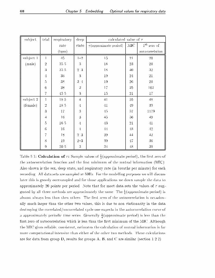
68 Chapter 5. Embedding | Optimal values for respiratory data
subject trial respiratory sleep calculated value of �
rate state 1
4(approximate period) MIC 1st zero of
(bpm) autocorrelation
subject 1 1 45 1{2 15 21 20
(male) 2 35.5 3 18 23 20
3 35.5 2{3 18 40 32
4 36 3 19 24 21
5 38 3{4 19 26 20
6 38 2 17 25 102
7 45.5 3 15 21 17
subject 2 1 18.5 4 41 55 48
(female) 2 18.5 4 41 49 39
3 17 3 45 57 1179
4 16 3 45 56 49
5 16.5 4 43 21 41
6 16 4 44 48 42
7 18 2{3 39 44 42
8 19 2{3 39 47 36
9 20.5 3 34 48 39
Table 5.1: Calculation of � : Sample values of 14(approximate period), the �rst zero of
the autocorrelation function and the �rst minimum of the mutual information (MIC).
Also shown is the sex, sleep state, and respiratory rate (in breaths per minute) for each
recording. All data sets are sampled at 50Hz. For the modelling purposes we will discuss
later this is grossly oversampled and for those applications we down sample the data to
approximately 20 points per period. Note that for most data sets the values of � sug-
gested by all three methods are approximately the same. The 14(approximate period) is
almost always less than then others. The �rst zero of the autocorrelation is occasion-
ally much larger than the other two values, this is due to non stationarity in the data
destroying the correlated/uncorrelated cycle one expects in the autocorrelation curve of
a approximately periodic time series. Generally 14(approximate period) is less than the
�rst zero of autocorrelation which is less than the �rst minimum of the MIC. Although
the MIC gives reliable, consistent, estimates the calculation of mutual information is far
more computational intensive than either of the other two methods. These calculations
are for data from group D, results for groups A, B, and C are similar (section 1.2.2).

5.3. Calculation of � 69
4
5
6 4.5 5 5.5
4
4.5
5
5.5
6
x1 x2
x3
(c)
4 4.5 5 5.5 64
4.5
5
5.5
6(a)
−10 −5 0 5 10−8
−6
−4
−2
0
2
4
6(b)
Figure 5.2: E�ect of � on the shape of an embedding: Panel (a) and (b) are
two dimensional embeddings of di�erent data sets, panel (c) is a (projection of a) three
dimensional embedding of the data of panel (a). The data (and choice of embedding lag)
for panel (a) and (c) are the same, panel (b) is a di�erent data set with a di�erent value of
embedding lag. Note the distinctive shape of (a) and (b). However, this is due primarily
to the choice of � (relative to r, see �gure 5.3 and shape of inspiratory/expiratory cycle.

70 Chapter 5. Embedding | Optimal values for respiratory data
r
1-r
1
0 100 200 300 400 500 600 700 800 900 10004
5
6
Figure 5.3: Parameter r: The parameter r is the fraction of the total time spent on
the expiratory phase of respiration. The data shown in the top panel is far from the
saw tooth waveform we approximate it by. This is the most extreme situation, and will
e�ectively add an extra phase to the dynamics of the embedded data | a section of
phase space with slow moving dynamics as all coordinates have similar values.

5.3. Calculation of � 71
D
A
D
BC
C
B
D
C
A
B
t
y
y
yy
y
y
ty
y
t t
A
t- τ τ
t- τ t- τ
t-
(i)
AB
C
D(ii)
(iii) (iv)
Figure 5.4: Dependence of shape of embedding on � and r: Panel (i), (ii), (iii),
and (iv) represent the four situations described in the text. Each section is denoted
(consistent with the text) by A, B, C, and D. Note that, for increasing values of �
(relative to r) the embedding produces a self intersection when 1 � r < � < r or
r < � < 1�r. Note that in panel (ii) and (iii) the simple periodic motion is not embeddedsatisfactorily in R2 | one has self intersections which a 3 dimensional embedding would
be required to remove (for those values of �).

72 Chapter 5. Embedding | Optimal values for respiratory data
r < � < 1� r; and (iv) r; 1� r < � . In normal respiration we have that r > 1� r and
increasing � will cause a transition from (i) to (ii) to (iv). We will now describe each of
these four situations, �gure 5.4 illustrates these results.
(i.) � < r; 1 � r. The two dimensional embedding will have four separate sections,
where
A: both the coordinates yt and yt�� are on the expiratory phase of the respira-
tory cycle.
B: yt is on the inspiratory phase and yt�� is on the preceding expiratory phase.
C: both yt and yt�� are on the inspiratory phase.
D: yt is on the expiratory phase and yt�� is on the preceding inspiratory phase.
(ii.) 1� r < � < r. The two dimensional embedding will have four separate sections,
namely
A: both the coordinates yt and yt�� are on the inspiratory phase of the respira-
tory cycle.
B: yt is on the expiratory phase and yt�� is on the preceding inspiratory phase.
C: yt is on a new inspiratory phase whilst yt�� is on the preceding inspiratory
phase.
D: yt is on the inspiratory phase and yt�� is on the preceding expiratory phase.
(iii.) r < � < 1� r. The two dimensional embedding will have four separate sections,
namely
A: both the coordinates yt and yt�� are on the expiratory phase of the respira-
tory cycle.
B: yt is on the inspiratory phase and yt�� is on the preceding expiratory phase.
C: yt is on a new expiratory phase whilst yt�� is on the preceding expiratory
phase.
D: yt is on the expiratory phase and yt�� is on the preceding inspiratory phase.
(iv.) 1� r; r < � . In this case the four sections are
A: yt is on the expiratory phase and yt�� is on the preceding inspiratory phase.
B: yt and yt�� are on successive inspiratory phases.
C: yt is on the new inspiratory phase and yt�� is on the preceding expiratory
phase.
D: yt and yt�� are on successive expiratory phases.

5.3. Calculation of � 73
Hence the embedding will generally have a rectangular appearance. However if
1� r < � < r or r < � < 1� r the embedded data will (in 2 dimensions) have crossings
of trajectories. In general one expects that r � 1�r and so if � is one quarter of a period(� = 0:25) this situation is avoided and one has an acceptable embedding. However,
if r � 14 or 1 � r � 1
4 then the embedding will be either be triangular (the case when
r = 14 or 1� r = 1
4) or have self intersections. Hence, when choosing an embedding we
should select � = 14(approximate period) and ensure that � < min(r; 1� r).

74 Chapter 5. Embedding | Optimal values for respiratory data

75CHAPTER 6
Nonlinear modelling
This chapter describes an attempt to accurately model the respiratory patterns of human
infants using new nonlinear modelling techniques. In chapters 2 and 5 we discussed
methods to reconstruct the attractor of a time series from data. Chapters 3 and 4
describe methods one may employ to deduce nonlinear determinism in experimental
data. In this chapter we describe necessary modi�cations to the modelling algorithm
described in section 2.3 and [62] to accurately model the nonlinear dynamics of the
human respiratory system. We have evidence to suggest the presence of nonlinearity in
the respiration of sleeping infants [136, 140]1. To produce adequate nonlinear models
we found that present methods (section 2.3) have to be improved substantially. This
chapter describes the author's improvements to the existing algorithm.
We have identi�ed periodic uctuation in regular breathing pattern of sleeping in-
fants using linear modelling techniques [133] (see chapter 9). An accurate, reliable and
replicable method of building nonlinear models may further aid the identi�cation of
such subtle periodicities and give some insight into the mechanisms generating them.
Just as a di�erential equation model of a system can lead to greater understanding,
so too can numerical, nonlinear models. The detection of this respiratory uctuation
is described in chapter 9. Chapter 7, 8 and 10 describe applications of the modelling
algorithm presented in this chapter.
Initially we used a radial basis modelling algorithm described by Judd and Mees [62]
to model recordings of the abdominal movements of sleeping infants. Although these
radial basis models give accurate short term predictions, they were not entirely satis-
factory in the sense that simulations of the models failed to exhibit some characteristics
of the original signals. After some alteration of the model building algorithm, much
better results were obtained; simulations of the models exhibit signals that are nearly
indistinguishable from the original signals.
In this chapter we �rst describe the time series we will model, a review of the
nonlinear modelling methods of Judd and Mees [62] may be found in section 2.3. We
identify some failings of simulations of models produced by this algorithm; suggest new
modi�cations that may overcome these problems; and �nally demonstrate the improved
results we have obtained.
We have used data collected from sleeping infants to estimate the correlation dimen-
sion of the respiratory patterns [136, 140], and to identify cyclic amplitude modulation
(CAM) in respiration during quiet sleep [133]. This work will be discussed in chapters 8
and 9. These studies concluded that linear modelling techniques were unable to model
the dynamics of human respiration2. Furthermore, by comparing the correlation dimen-
1This work is presented in chapter 8.2By calculating correlation dimension dc("0) for data embedded in R3, R4 and R5 as a test statistic
surrogate analysis of 27 recordings of infant respiration from 10 infants concluded that the data were

76 Chapter 6. Nonlinear modelling
160 180 200 220 240 260 280 300 320−5
0
5
10
time(seconds)
Abd
. Are
a
Figure 6.1: Data: The data we use in our calculations. The solid line represents the
data set from which we build our radial basis models. The horizontal axis is time elapsed
from the start of data collection and the vertical axis is the output from the analogue to
digital convertor (proportional to cross-sectional area measured by inductance plethys-
mography). Note the sigh (at about 300 seconds) and the onset of periodic breathing
following this. The data represented as a solid line is also shown in �gure 4.5 and is
from group A (section 1.2.2).
sion estimates for the data and surrogates we were able to demonstrate that simulations
from radial basis models produced dimension estimates that closely resembled that of
the data (chapter 8). This implies that nonlinear models are more accurately modelling
the data than are linear models. However, these nonlinear models appeared to have
di�culty with some data sets, most notably those with substantial noise contamina-
tion and data exhibiting non-stationarity. In this section we attempt to improve the
modelling techniques.
6.1 Modelling respiration
In this section we introduce the data set that we will attempt to model. In chapter
2.1 we described the use of correlation dimension estimation and false nearest neighbour
techniques to determine a suitable embedding dimension and examined three alterna-
tive criteria for embedding lag to deduce an appropriate value. Sections 5.2 and 5.3
demonstrated the calculation of typical values of de and � for reconstruction via time
delay embedding. In the following section we brie y describe the data we will exam-
ine in this chapter. In section 6.1.2 we use these embedding techniques to reconstruct
the dynamical system from these data and apply the nonlinear modelling technique
described in section 2.3 and examine the weaknesses of the result.
6.1.1 Data For much of the following sections we illustrate the calculation and
comparison using just one recording, selected because it is a \typical" representation of
a range of important dynamical features. The data set we use (see �gure 6.1) is from a
inconsistent with each of the linear hypotheses addressed by Theiler and colleagues [152].
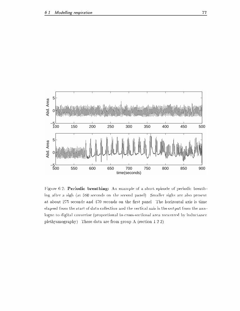
6.1. Modelling respiration 77
500 550 600 650 700 750 800 850 900−5
0
5
time(seconds)
Abd
. Are
a
100 150 200 250 300 350 400 450 500−5
0
5
Abd
. Are
a
Figure 6.2: Periodic breathing: An example of a short episode of periodic breath-
ing after a sigh (at 580 seconds on the second panel). Smaller sighs are also present
at about 275 seconds and 470 seconds on the �rst panel. The horizontal axis is time
elapsed from the start of data collection and the vertical axis is the output from the ana-
logue to digital convertor (proportional to cross-sectional area measured by inductance
plethysmography). These data are from group A (section 1.2.2).

78 Chapter 6. Nonlinear modelling
section of approximately 10 minutes of respiration of a two month old female in quiet
(stage 3{4) sleep. These data exhibits a physiological phenomenon of great interest
to respiratory specialists known as periodic breathing [66, 85]. Periodic breathing is
simply extreme CAM | the minimum amplitude decreases to zero. Figure 6.2 shows
an example of periodic breathing. In all other respects these data are typical of many
of our recordings. The section which we examine �rst is from a period of quiet sleep
preceding the onset of periodic breathing (see �gure 6.1). All data used in this chapter
is from group A (section 1.2.2).
6.1.2 Modelling We attempt to build the best model of the form
yt+1 = f(zt) + "t
where "t is the model prediction error and f : Rd 7! R is of the form
f(zt) = �0 +nXi=1
�iyt�`i +mXj=1
�j+n+1�
�kzt � cjkrj
�; (6.1)
where rj and �j are scalar constants, 1 � `i < `i+1 � d� are integers and cj are arbitrary
points in Rd. The integer parameters n and m are selected to minimise the description
length [110] as described in [62]. Here �(�) represents the class of radial basis functionfrom which the model will be built. We choose to use Gaussian basis functions because
they appear to be capable of modelling a wide variety of phenomena. This model, and
an algorithm to �t it to data, have been described in section 2.3.
The data set consists of 20000 points sampled at 50Hz. This is oversampled for our
purposes and we thin the data set to one in four points and truncate it to a length of
1600 (see �gure 6.1). Using the techniques of section 2.1 and the results of sections 5.2
and 5.3, we set d = 4 and choose � = 5.
Trials with the modelling algorithm as described in [62] produced some problems
with the model simulations (see �gure 6.3). None of the simulations look like the data.
When periodic orbits are evident they are still unlike the data; the waveform is sym-
metric, whereas the data have a de�nite asymmetry. Moreover the free run predictions
from these models often exhibit stable �xed points. This is extremely undesirable as it
is evidently not an accurate representation of the dynamics of respiration | breathing
does not tend to a �xed point, usually.
The remainder of this chapter shall be concerned with addressing these problems.
These problems are the result of three main de�ciencies in the initial modelling algo-
rithm: (i) it over �ts the data; (ii) it does not produce appropriate simulations; and
(iii) models are not consistent or reproducible. We will attempt to improve upon these
problems whilst considering the many competing criteria for a good model.

6.2. Improvements 79
0 100 200 300 400−2
0
2
Abd
. Are
a
Abd
. Are
a
t t
Simulation
0 100 200 300 400−2
0
2Free run prediction
Figure 6.3: Initial modelling results: Free run prediction and noise driven simulation
of a radial basis model. The plot on the left is a free run prediction with no noise, on the
right is a simulation driven by Gaussian noise at 10% of the root-mean-square prediction
error (qPt
i=1 "2i =pN). The horizontal axis is yt for t = 1; : : : ; 500, the vertical axis is
the output from the analogue to digital convertor (proportional to cross-sectional area
measured by inductance plethysmography). From 30 trials 27 of them exhibited �xed
points.
6.2 Improvements
Before we can attempt to improve our modelling procedure we must be clear on
what we mean by improvement. There are several criteria that might be imposed to
achieve a \good" model.
Modelling criteria measure quantities such as the number of parameters in the model,
its prediction error and description length. It is desirable to have a model with few
parameters, a small description length and a small root mean square prediction error.
Algorithmic criteria are concerned with optimising the modelling algorithm, to en-
sure that it searches the broadest possible range of basis functions as e�ciently as
possible. Unfortunately a larger search space comes at the expense of more computa-
tion.
Qualitative criteria consider properties of the dynamics of models; for example, the
behaviour observed in the simulations of the model. In modelling breathing, for example,
we expect something like stable periodic (or quasi-periodic) solutions; divergence or
stable �xed points seem unlikely. Furthermore, we expect the shape of the periodic
solution to closely match the shape of the data and to occupy the same region of phase
space.
Modelling results should also be reproducible and representative. It does not seem
unreasonable to expect consistent, repeatable results from a modelling algorithm, both
qualitatively and quantitatively. Reproducibility can be examined by repeatedly mod-
elling a single data set. Furthermore, the model should be representative in that when
making many simulations of the model, we ought to obtain time series of which the
original data are representative. Representativity can be measured with the assistance
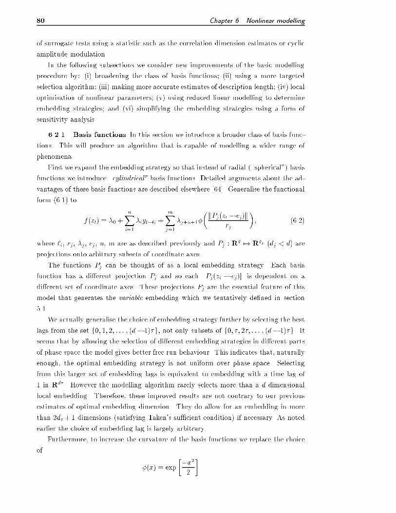
80 Chapter 6. Nonlinear modelling
of surrogate tests using a statistic such as the correlation dimension estimates or cyclic
amplitude modulation.
In the following subsections we consider new improvements of the basic modelling
procedure by: (i) broadening the class of basis functions; (ii) using a more targeted
selection algorithm; (iii) making more accurate estimates of description length; (iv) local
optimisation of nonlinear parameters; (v) using reduced linear modelling to determine
embedding strategies; and (vi) simplifying the embedding strategies using a form of
sensitivity analysis.
6.2.1 Basis functions In this section we introduce a broader class of basis func-
tions. This will produce an algorithm that is capable of modelling a wider range of
phenomena.
First we expand the embedding strategy so that instead of radial (\spherical") basis
functions we introduce \cylindrical" basis functions. Detailed arguments about the ad-
vantages of these basis functions are described elsewhere [64]. Generalise the functional
form (6.1) to
f(zt) = �0 +nXi=1
�iyt�`i +mXj=1
�j+n+1�
�kPj(zt � cj)krj
�; (6.2)
where `i, rj, �j , cj , n, m are as described previously and Pj : Rd 7! Rdj (dj < d) are
projections onto arbitrary subsets of coordinate axes.
The functions Pj can be thought of as a local embedding strategy. Each basis
function has a di�erent projection Pj and so each kPj(zt � cj)k is dependent on a
di�erent set of coordinate axes. These projections Pj are the essential feature of this
model that generates the variable embedding which we tentatively de�ned in section
5.1.
We actually generalise the choice of embedding strategy further by selecting the best
lags from the set f0; 1; 2; : : : ; (d� 1)�g, not only subsets of f0; �; 2�; : : : ; (d� 1)�g. Itseems that by allowing the selection of di�erent embedding strategies in di�erent parts
of phase space the model gives better free run behaviour. This indicates that, naturally
enough, the optimal embedding strategy is not uniform over phase space. Selecting
from this larger set of embedding lags is equivalent to embedding with a time lag of
1 in Rd� . However the modelling algorithm rarely selects more than a d dimensional
local embedding. Therefore, these improved results are not contrary to our previous
estimates of optimal embedding dimension. They do allow for an embedding in more
than 2dc + 1 dimensions (satisfying Taken's su�cient condition) if necessary. As noted
earlier the choice of embedding lag is largely arbitrary.
Furthermore, to increase the curvature of the basis functions we replace the choice
of
�(x) = exp
��x22
�

6.2. Improvements 81
by
~�(x; %) = exp
�(1� %)
x%
%
�
where 1 < % < R is the curvature3 and 1�%% is a correction factor so that 1p
2�
R1�1 ~�(x; %)dx=
1. Hence, maintaining consistent notation
~�(x; %) = �
s2(1� %)
%x%2
!;
and the basis functions become functions of the form
�
s2(1� %j)
%j
kPj(zt � cj)krj
%j2
!
where
�(x) = exp�x22
:
Broadening the class of basis functions has increased the complexity of the search
algorithm. Hopefully it will also have broadened the search space su�ciently to encom-
pass functions which can more accurately model the data. To overcome this increased
search space we consider a more e�cient search algorithm.
6.2.2 Directed basis selection The method of Judd and Mees [62] involves
randomly generating a large set of basis functions f�(kz�cjkrj)gj = f�jgj and evaluating
them at each point of the embedded time series z to give the matrix V = [�1j�2j � � � j�M ].
Following an iterative scheme they repeatedly select columns from this matrix (and the
corresponding candidate basis function) to add to the optimal model. This is the model
selection algorithm described in section 2.3.3.
Instead, we select a new set of candidate basis functions f�jgj (and a new matrix
V ) at each expansion of the optimal model. We then identify the column k of V
that best �ts the residuals (orthogonal to the previously selected basis functions) and
select the corresponding basis function �k . All the other candidate basis functions
f�jgj=1;::: ;M ;j 6=k are ignored and forgotten at the next iteration. Because a new set
of basis functions are selected at each expansion, all the candidate basis functions are
much more appropriately placed4. We have the following algorithm.
Algorithm 6.1: Revised model selection algorithm.
1. Normalise the columns of V to have unit length.
3To prevent large values of the second derivative of f it is necessary to provide an upper bound R
on %.4Basis functions are selected according to either a uniform distribution or the probability distribution
induced by the magnitude of the modelling prediction error.

82 Chapter 6. Nonlinear modelling
2. Let S0 = (�N2 � 1) ln(yTy= �N) + 1
2 + ln . Let eB = y and VB = ;.3. Let � = V T eB and j be the index of the component of � with maximum
absolute value. Let V 0B = VB [ fVjg.
4. Generate a new matrix V containing a new set of candidate basis func-
tions fVigmi=1. Normalise V .5. Calculate �B0 so that y � VB�B0 is minimised. Let �0 = V TeB0 . Let o
be the index in B0 corresponding to the component of �0 with smallest
absolute value.
6. If o 6= jVBj, then put VB = V 0B n fVog, calculate �B so that y� VB�B is
minimised, let eB = y � VB�B, and go to step 3.
7. De�ne Bk = VB, where k = jVBj. Find � such that (V TB VB�)j = 1=�j
for each j = f1; : : : ; kg and calculate Sk = (�N2 �1) ln
eTBeB�N
+(k+1)(12+
ln )�Pkj=1 ln �̂j .
8. If some stopping condition has not been meet, then go to step 3.
9. Take the basis Bk such that Sk is minimum as the optimal model.
Note that the explication of this algorithm contains a slight abuse of notation, VB
is both the set of basis functions fVjgkj=1 and the matrix [V1jV2j � � � jVk]. Note that,
the essential di�erence between this and algorithm 2.1 is that step 4 generates a new
set of candidate basis functions each time. As a consequence it is necessary to keep
track of the basis functions in the model VB5, and not just indices B. The improvement
in modelling achieved by this will require greater computation time. Furthermore the
selection of basis functions that more closely �t the data may, possibly, increase the
number of basis functions allowed by the description length criterion. To alleviate this
problem we introduce a harsher more precise version of description length.
6.2.3 Description length The minimum description length criterion, suggested
by Rissanen [110], is used by Judd and Mees [62] to prevent over �tting. This is the
description length criterion described in section 2.3.2. However, the original implemen-
tation of minimum description length used by Judd and Mees only provides a descrip-
tion length penalty for the coe�cient �j of each of the radial basis functions (and linear
terms). Each basis function also has a radius rj and coordinates cj which must also be
speci�ed to some precision, and hence should also be included in the description length
calculation.
In [62] �j is �j truncated to some �nite precision �j , then the description length is
expressed as
L(z; �) = L(zj�) + L(�) (6.3)
5In practice one will need to record the parameters which determine these basis functions.

6.2. Improvements 83
where
L(zj�) = � ln P (zj�)
is the description length of the model prediction errors (the negative log likelihood of
the errors) and
L(�) �m+n+1Xj=1
ln
�j
is the description length of the truncated parameters, is an inconsequential constant.
We generalise equation (6.3) and include the �nite precisions of rj and cj . Let �
represent the vector of all the model parameters (�j, cj , and rj) and � the truncation
of those parameters to precision �. Then
L(z;�) = L(zj�) + L(�) (6.4)
where
L(�) �(d+2)m+n+1X
j=1
ln
�j:
Now the problem becomes one of choosing � to minimise (6.4). By assuming that
� is not far from the maximum likelihood solution �̂ (see section 6.2.4) one can deduce
that
L(z;�) � L(zj�̂) + 1
2�TQ�+ k ln �
kXj=1
ln �j ; (6.5)
where k = ((d+ 2)m+ n+ 1). Minimising (6.5) gives (as in [62]),
(Q�)j = 1=�j
where Q = D��L(zj�) is the second derivative of the negative log likelihood, with
respect to all the parameters.
Although algebraically complicated, this expression can be solved relatively e�-
ciently by numerical methods. However, by assuming that the precision of the radii and
the position of the basis function must be approximately the same6, one can circumvent
a great deal of the computational di�culty, and simply calculate the precision of rj |
assuming the same values for the corresponding precisions of the coordinates cj .
Much of the computational complexity of calculating description length could be
avoided by utilising the Schwarz criterion (2.15). Indeed, from experience it appears that
the Schwarz criterion gives comparable size models. However, Schwarz' criterion does
not take into account the relative accuracy of di�erent basis functions | an important
feature of minimum description length.
6Since a slight change in radius will a�ect the evaluation of a basis function over phase space in the
same way as an equal small change in the position of the basis function.

84 Chapter 6. Nonlinear modelling
6.2.4 Maximum likelihood Once the best (according to sensitivity analysis)
basis function has been selected we improve on its placement by attempting to maximise
the likelihood
P (zj�; �2) = 1
(2��2)N=2exp
(y � V �)T (y � V �)
2�2
where y � V � = " is the model prediction error, and �2 is the variance of the (assumed
to be) Gaussian error. By setting �2 =Pt
i=1 "2i =N and taking logarithms one gets that
lnP (zj�) = N
2+ ln
�2�
N
�N=2
+ ln
tX
i=1
"2i
!N=2
: (6.6)
To maximise the likelihood we optimise equation (6.6) by di�erentiating
ln (tX
i=1
"2i )N=2
with respect to rj , cj , and �j . This calculation is algebraically messy, but computation-
ally straightforward provided a good optimisation package is used7.
6.2.5 Linear modelling selection of embedding strategy Allowing di�erent
embedding strategies from such a wide class (due to the expansion of the class of basis
functions in section 6.2.1) increases the computational complexity of the modelling
process. However, to circumvent this we note that for Gaussian basis functions the �rst
order Taylor Series expansion gives
�
�kPj(zt � cj)krj
�= �
0@qPd�
i=1 pi(zt � cj)2
rj
1A
�d�Xi=1
�
� jpi(zt � cj)jrj
�(6.7)
where pi : Rd� 7! R is the coordinate projection onto the i-th coordinate. We then
build a minimum description length model of the residual of the form (6.7). That
is, we select the columns ofh�� jpi(zt�cj)j
rj
�id�i=1
which yield the model with minimum
description length. From this we deduce that the basis functions selected are a good
indication of an appropriate embedding strategy. Hence, if the minimum description
length model consists of the basis functions��
� jp`(zt � cj)jrj
��`2f`1;`2;::: ;`dj g
then we use the embedding strategy f`1; `2; : : : ; `djg. Although this method is ap-
proximate it is hoped that this will provide useful and e�cient innovation within the
modelling algorithm.
7Many potentially useful optimisation packages are available via the internet. At the time of
writing this thesis, a list of public domain and commercial optimisation routines was available
from the URL http://www.isa.utl.pt/matemati/mestrado/io/nlp.html, and from the newsgroup
sci.op-research. In this thesis the author uses an algorithm by Powell [97, 99].
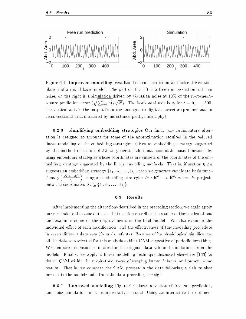
6.3. Results 85
0 100 200 300 400−2
0
2
Abd
. Are
a
Abd
. Are
a
t t
Simulation
0 100 200 300 400−2
0
2Free run prediction
Figure 6.4: Improved modelling results: Free run prediction and noise driven sim-
ulation of a radial basis model. The plot on the left is a free run prediction with no
noise, on the right is a simulation driven by Gaussian noise at 10% of the root-mean-
square prediction error (qPt
i=1 "2i =pN). The horizontal axis is yt for t = 0; : : : ; 500,
the vertical axis is the output from the analogue to digital convertor (proportional to
cross-sectional area measured by inductance plethysmography).
6.2.6 Simplifying embedding strategies Our �nal, very rudimentary alter-
ation is designed to account for some of the approximation required in the reduced
linear modelling of the embedding strategies. Given an embedding strategy suggested
by the method of section 6.2.5 we generate additional candidate basis functions by
using embedding strategies whose coordinates are subsets of the coordinates of the em-
bedding strategy suggested by the linear modelling methods. That is, if section 6.2.5
suggests an embedding strategy f`1; `2; : : : ; `djg then we generate candidate basis func-
tions �� jPi(zt�cj)j
rj
�using all embedding strategies Pi : R
d 7�! Rdi where Pi projects
onto the coordinates Xi � f`1; `2; : : : ; `djg.
6.3 Results
After implementing the alterations described in the preceding section, we again apply
our methods to the same data set. This section describes the results of these calculations
and examines some of the improvements in the �nal model. We also examine the
individual e�ect of each modi�cation. and the e�ectiveness of this modelling procedure
in seven di�erent data sets (from six infants). Because of its physiological signi�cance,
all the data sets selected for this analysis exhibit CAM suggestive of periodic breathing.
We compare dimension estimates for the original data sets and simulations from the
models. Finally, we apply a linear modelling technique discussed elsewhere [133] to
detect CAM within the respiratory traces of sleeping human infants, and present some
results. That is, we compare the CAM present in the data following a sigh to that
present in the models built from the data preceding the sigh.
6.3.1 Improved modelling Figure 6.4 shows a section of free run prediction,
and noisy simulation for a \representative" model. Using an interactive three dimen-

86 Chapter 6. Nonlinear modelling
Figure 6.5: Cylindrical basis model: A pictorial representation of the interactive
3 dimensional viewer we used. The axes range from �1:715415 to 3:079051, the
same range of values as the data. The point (�1:7;�1:7;�1:7) is in the front cen-
tre, foreground. The cylinders, prisms and sphere represent the placement (cj) and
size (rj) of di�erent basis functions with di�erent embedding strategies: the X , Y ,
and Z coordinates shown correspond to yt, yt�5, and yt�15 respectively. The colour-
ing of the basis functions represents the value of the coe�cients (�j). This repre-
sentation will be discussed in more detail in section 7.1. The corresponding URL is
http://maths.uwa.edu.au/�watchman/thesis/vrml/3Dmodel.vrml.

6.3. Results 87
Abd
. Are
a
time (seconds)0 20 40 60 80 100 120 140 160 180 200
−1.5
−1
−0.5
0
0.5
1
1.5
Figure 6.6: Short term behaviour: Comparison of simulation and data. The solid
line for the data, the dot-dashed is a free run prediction, the dashed is a simulation
driven by noise (20% ofqPt
i=1 "2i =pN). The initial conditions for the arti�cial sim-
ulations are identical and are taken from the data. The vertical axis is the output
from the analogue to digital convertor (proportional to cross-sectional area measured
by inductance plethysmography).
sional viewer (see �gure 6.58) it is possible to determine that these models also have
many more common structural characteristics than those created in section 6.1.2. The
size, placement, shape and local embedding dimensions of the basis functions of the
models have many similarities. Some observations regarding the physical characteris-
tics of these models is presented in section 7.1
Importantly, all of these models have similar free run behaviour. The free run
predictions are as large (in amplitude) as the data; this was a substantial problem
with the original modelling procedure. Moreover, the free run behaviour with noise
appears more \realistic" and the shape of the simulations mimic very closely that of
the data. Figure 6.6 shows a short segment of a simulation, along with the data. Note
the similarities in the shape of the prediction and the data. Finally, the simulations
exhibit a measurable cyclic amplitude modulation which we use in section 6.3.3 to infer
the presence of cyclic amplitude modulation in the original time series.
8All the three dimensional �gures represented in this thesis are also available on the inter-
net as three dimensional object �les. An index of all these �gures is currently accessible at
http://maths.uwa.edu.au/�watchman/thesis/vrml/vrmls.html.

88 Chapter 6. Nonlinear modelling
Modelling
nonlinear
RMSerror
MDL
Freerun
CPUtime
method
parameters �qPti=
1"2i = pN �
amplitude
(seconds)
A
12.5�2.4
0.135�0.016
-1086�157
0.00�0.91
155.7�61.88
A+B
12.5�2.4
0.113�0.011
-1090�155
1.22�31.90
152.7�57.08
A+B+C
24.5�4.3
0.104�0.015
-1123�198
1.58�1.04
308.4�94.74
A+B+D
10.7�2.3
0.122�0.016
-975�191
0.34�24.91
391.2�295.2
A+B+C+D
14.5�3.5
0.123�0.018
-909�210
1.50�1.09
781�540.8
A+B+C+D+E
9.5�2.9
0.141�0.012
-735�131
1.59�1.31
1152�851.9
A+B+C+D+F
13.7�3.6
0.126�0.009
-870�81
1.31�17.48
2773�1100
A+B+C+D+E+F
11.0�3.1
0.117�0.013
-990�119
1.17�17.94
2945�1294
A+B+C+D+E+F+G
11.4�3.2
0.117�0.011
-980�110
1.87�1.00
2663�944.9
Table6.1:Algorithmicperformance:Comparisonofthemodellingalgorithmwithvarious\improvements".Thesevendi�erentmodelling
proceduresaretheinitialroutinedescribedbyJuddandMees,andsixalterationsdescribedinsection6.2.Modellingmethodsare:(A)the
initialmethod;(B)extendedbasisfunctionsandembeddingstrategies;(C)directedbasisselection;(D)exactdescriptionlength;(E)local
optimisationofnonlinearmodelparameters;(F)reducedlinearmodellingtoselectembeddingstrategies;and(G)simplifyingembedding
strategies.Resultsarefrom
30attemptsatmodellingdatadescribedinsection6.1.1and�gure6.1.Thenumbersquotedare(mean
value)�(standarddeviation).CalculationswereperformedonaSiliconGraphicsIndyrunningat133MHzwith16MbytesofRAM.These
calculationsareidenticaltothoseof[135],exceptthattheCPUtimehasbeenrecalculatedonaSiliconGraphics02(180MHzclockspeedwith
64MbytesofRAM)fordirectcomparisontotheresultsoftable6.3.CPUtimeismeasureinsecondsusingMATLAB'scputimecommand.

6.3. Results 89
6.3.2 E�ect of individual alterations Table 6.1 lists some characteristics of
models built from the data in �gure 6.1 using various methods. The di�erent modelling
strategies are: (A) the initial method (described in section 6.1.2); (B) extended basis
functions and embedding strategies (section 6.2.1); (C) directed basis selection (6.2.2);
(D) more accurate approximation to description length (6.2.3); (E) local optimisation of
nonlinear model parameters (6.2.4); (F) reduced linear modelling to select embedding
strategies (6.2.5); and, (G) simplifying embedding strategies (6.2.6). These alterations
to the algorithm were progressively added in various combinations and characteristics
of the observed models measured.
The initial procedure (A) produced very bad free run predictions; 27 out of 30 trials
produced simulations with �xed points. Extending the class of basis functions and
adding cylindrical basis functions (B) vastly improved this (only 8 out of 30 simulations
did not have periodic (or quasi-periodic) orbits). Most of the periodic orbits in these
simulations were smaller than the data (did not occupy the same part of phase space)
and one divergent simulation was observed (hence the large standard deviation in table
6.1). This approach decreased the prediction error without a�ecting either the model
size or description length (clearly, the required precision of the parameters was greater).
Directed basis selection (C) greatly increased the size of the model and decreased
error whilst improving free run behaviour | not only in amplitude but also shape.
The increase in computational time could almost entirely be due to the greater model
size. Improving the description length calculation (D) decreased the model size whilst,
predictably increasing prediction error. This also caused a surprising increase in calcu-
lation time | an indication of the computational di�culty solving (Q�)j = 1=�j when
Q is the second derivative with respect to all the model parameters (or at least � and
r). Because there is a harsh penalty these models are far less likely to be over �tting
the data. Combining the improved description length calculation and directed basis
selection produced models comparable in both size and �tting error to before either al-
teration was implemented (A+B). However, free run behaviour had an amplitude closer
to the mean amplitude of the data and exhibited an asymmetric waveform similar to
the data.
Addition of the nonlinear optimisation (E) and local linear modelling (F) routines
caused the greatest increase to computational time. Individually these methods did
not o�er any considerable improvement to the other model characteristics. However
many of the statistics indicate a decrease in the variation between trials. Combined,
these modi�cations gave a slight improvement in prediction error and description length
whilst making the model smaller. They produced more realistic simulations although
the amplitude was smaller than that of the data.
Finally, the simple procedure of checking that simpler embedding strategies would
not produce better (or equally good) results (G) caused a substantial improvement.
This is perhaps due in part to the previous optimisation and local linear methods, par-

90 Chapter 6. Nonlinear modelling
450 500 550 600 650 700−10
−5
0
5
10
time (sec)
Abd
. Are
a
subjectM
Figure 6.7: Periodic breathing: An example of periodic behaviour in one of our data
sets. The solid region was used to build a nonlinear radial basis model. Note that
periodic breathing begins immediately after the sigh. The vertical axis is the output
from the analogue to digital convertor (proportional to cross-sectional area measured
by inductance plethysmography). These data are also illustrated as part of a longer
recording in �gure 6.2.
ticularly the approximate nature of the local linear modelling. Removing coordinates
helped produce some appreciable improvement in suitability of the embedding strate-
gies suggested by the approximate local linear methods. The local linear methods often
produce a high dimensional local embedding (many signi�cant coordinates); eliminat-
ing some of these will usually only slightly increase the prediction error. This simple
addition increases the amplitude to a realistic level (approximately 1:9 whilst the mean
breath size for the data is about 2:3 9) whilst decreasing the proportion of �xed point
and divergent trajectories to the lowest level (8 and 0 of the 30 models, respectively)
without appreciably changing the description length, prediction error, or model size
whilst decreasing slightly the calculation time (and variance in calculation time). Fur-
thermore, these models have far more structural similarities (in the size and placement
of basis functions) than the previous models have, indicating that these model are far
more consistent.
The remainder of this section is devoted to some applications of these modelling
methods and tests of their representability.
6.3.3 Modelling results From over 200 recordings of 19 infants, we identi�ed
seven data sets from six infants for more careful analysis. All seven of these data sets
include a sigh followed by a period of breathing exhibiting cyclic amplitude modulation
(CAM). Our present discussion examines the analysis of these data sets.
In this section we examine the free run behaviour of data sets created from seven
models of seven data sets from six sleeping infants. We compare the correlation dimen-
9Note, however that the data are slightly non-stationary whilst the model is not. Non-stationary
models of this data are described in section 7.4.

6.3. Results 91
sion of the data and simulations from models. Following this we compare the period
of CAM detected in the free run predictions from the models to that visually evident
after a sigh. Figure 6.7 illustrates one of the data sets used in our analysis. This is
the only set of data to exhibit periodic breathing, the others merely exhibited strong
amplitude modulation after the sigh for 25{60 seconds (� 15{30 breaths). Nevertheless
the change that the respiratory system undergoes after a large sigh is of great interest to
respiratory physiologists. We examine the system before and after a sigh to determine
evident physiological similarities in the mechanics of breathing.
For each of our seven data sets, we identify the location of the sigh, and extract data
sets of 1501 points spanning 120 seconds preceding the sigh. From these data sets the
respiratory rate of each recording was established and the period of respiration deduced.
Each data set was embedded in R4 with a lag equivalent to the integer closest to one
quarter of the approximate period. We then applied our modelling algorithm.
Surrogate analysis To determine exactly how similar data and model simulations are
we employ an obvious generalisation of the surrogate data analysis used by Theiler [152].
The principle of surrogate data is discussed in chapter 3 and 4.
In the present context, we are not interested in determining what type of system
generated the data | at least not at present. A simpler null hypothesis (for example
[151, 154]) consistent with the data does not concern us here. What is of greater
interest to us is determining if the models really do behave like the data. By calculating
models and generating free-run predictions from those models, we are in fact generating
surrogate data. The similarity of the value of various statistics applied to data and
surrogate can be used to gauge the accuracy of the model. Figure 6.8 shows calculations
of correlation dimension estimates (following the methods of Judd [60, 61]) for data and
surrogate.
Our calculations indicate a very close agreement between the correlation dimension
of the data and that of the simulations. In 6 of the 7 data sets the correlation dimension
estimate dc("0) for the data is within two standard deviations of the mean value of dc("0)
estimated from the ensemble of surrogates for all values of "0 for which both converged.
In the remaining data set the value of correlation dimension di�ered by more than 2
standard deviations only at the smallest values of "0 (the �nest detail in the data).
In all calculations dc("0) for the data is within three standard deviations of the mean
value of dc("0) estimated from the ensemble of surrogates. With respect to correlation
dimension our models are producing results virtually indistinguishable from the data.
Detection of CAM Previously [133] we have used a form of reduced autoregressive
modelling (RARM) to detect CAM in the regular breathing of infants during quiet
sleep (this will be discussed in chapter 9). We apply nonlinear modelling methods here
with two aims in mind: to demonstrate the accuracy of our modelling methods; and
to further demonstrate that CAM evident during periodic breathing and in response to
apnea or sigh is also present during quiet, regular breathing.

92 Chapter 6. Nonlinear modelling
−3 −2 −1 02
3
4
5
(nor
mal
ised
) dc
de=4; lag=7.−2.5 −2 −1.5 −1 −0.52
3
4
(nor
mal
ised
) dc
de=3; lag=7.
−2 −1.5 −1 −0.5 02
4
6
8
(nor
mal
ised
) dc
Bs2t8
de=5; lag=7.
−3 −2 −1 0 11
2
3
(nor
mal
ised
) dc
de=3; lag=10.
−2 −1 0 11
2
3
4(n
orm
alis
ed)
dc
de=4; lag=10.
−2 −1 0 11
2
3
4
(nor
mal
ised
) dc
Ms1t6
de=5; lag=10.
Figure 6.8: Surrogate calculations: Comparison of dimension estimates for data
and surrogates. The three �gures on the left are dimension estimates (for embedding
dimension from 3 to 5, shown from top to bottom) for a model of Bs2t8. The right
three plots are similar results for a model of Ms1t6. All surrogates are simulation
driven by Gaussian noise with a standard deviation of half the root mean square one
step prediction error. Each picture contains one dimension estimate for the data (solid
line), and thirty surrogates (dotted). The two data sets used in these calculations are
shown in �gures 6.1 and 6.7, respectively.

6.4. Problematic data 93
subject sex age model CAM in free run CAM after sigh
(months) size (breaths) (seconds) (breaths) (seconds)
A(As4t2) male 6 8(7) 5{6y 14y 5 25
Bb(Bs2t8) female 2 7(6) 6 9 6 9
Bb(Bs3t1) 6(5) 5 10 5 10
G(Gs2t4) female 2 4(3) 5 11 5 9
H(Hs1t2) male 1 5(3) 8{9y 11y 9 13
M(Ms1t6) female 1 6(4) none none 5 14.5
R(Rs2t4) male 2 8(6) 9 18 8 16
Table 6.2: Periodic behaviour: Comparison of CAM after apnea (apparent to visual
inspection), the second set of results, and CAM detected in the models limit cycle,
the �rst set of results. Data sets Ms1t6 and Bs2t8 exhibited periodic breathing. For
each data set marked cyclic amplitude modulation (CAM) occurred after a sigh and
was measured by inspection. Radial basis models were built on a section of quiet sleep
preceding the sigh, noise free limit cycles exhibited periodicities that were measured
in both time and breaths from the simulation. Limit cycles marked with a y were notstrictly periodic but rather exhibited a chaotic behaviour. Model size is m+ n(m), see
equation 6.2.
We have built nonlinear models following the methods outlined in this paper of
the regular respiration of six sleeping infants immediately preceding seven sighs and
the consequential onset of periodic or CAM respiration. For each of these models we
produce simulations both driven by Gaussian noise, and without noise. The noiseless
simulations approach a stable periodic (or chaotic, quasi-periodic) orbit which may
exhibit slight CAM. Table 6.2 summarises the results of these calculations.
In all but one data set CAM was present in the free run prediction of the nonlinear
model. The absence of CAM in one model may either indicate a lack of measurable
CAM in the data or a poor model (these data are illustrated in �gure 6.7). All other
data sets produced nonlinear models that exhibited CAM, the period of which matched
that observed after a sigh during visually apparent CAM.
6.4 Problematic data
Even using the new modelling improvements suggested here some data will produce
results which are inadequate. Usually the noise driven simulations or the free run
predictions will be unsatisfactory. In these situations it is usually a problem with the
model being unable to reproduce the form of the noise of the original system. The
model assumes i.i.d. Gaussian noise. The noise may be non-Gaussian, or non-identically
distributed.

94 Chapter 6. Nonlinear modelling
6.4.1 Non-Gaussian noise Although the modelling algorithm described above
assumes additive noise of the form N(0; �2) an adequate �t may be produced for data
with non-normal errors. In such a situation it is necessary to then estimate the distribu-
tion of prediction errors from the model and use this estimate to generate noise according
to the assumed distribution. Having estimated the distribution P (e) = Prob(�t < e)
(following the methods described by Silverman [127]) one may generate random variates
�t � P (e) as follows. Ensure that the distribution is bounded �t 2 [a; b] and generate
(e0; p0) 2 [a; b]� [0; 1] uniformly. If p0 � P (e0) then let � = e0 otherwise, select a new
pair (e0; p0) 2 [a; b]� [0; 1].
6.4.2 Non-identically distributed noise If the noise source is not i.i.d. then
the problem is not only to estimate the distribution p(e) but to estimate the ensemble
of state space dependent distributions p(e; v) = Prob(�t < ejvt = v). A substantial
simpli�cation to this problem is introduced in [140] (see chapter 8) to produce su�ciently
accurate results. One simply assumes �t � N(0; �(vt)2) and then only needs to estimate
�(vt).
6.5 Genetic algorithms
Genetic algorithms (GA) are a stochastic approach to optimisation of an objective
function, without calculating the derivative of that function. They are loosely analogous
to the concepts of inheritance, evolution and survival of the �ttest. Because these
algorithms do not require the evaluation of the derivative of an objective function they
may be particularly useful to �t a radial basis model to a data set. First we will review
the general idea of genetic algorithms and describe the application of this approach to
our modelling problem.
6.5.1 Review There are many introductory texts in mathematics and computer
science which cover the theory and application of genetic algorithms (for example [15,
86, 109]). We will brie y review the main ideas in this method. Given the general
optimisation problem.
max f(x)
subject to x 2 X
a genetic algorithm will perform a stochastic search of X for an optimum value of f . Let
G0 � X be an initial population of candidate solutions. From Gk a genetic algorithm
will generate a new population Gk+1 according to simple rules analogous to the basic
concepts of inheritance, breeding, and mutation. Hence, Gk is called the kth generation.
To do this one works not in the space X but in some representation X̂ of that
space. One requires that there exists a bijective map m : X 7�! X̂ such that for all
x 2 X the representation m(x) consists of a �xed �nite number of symbols from a �nite
alphabet. For example an n place binary representation would consist of a string of n

6.5. Genetic algorithms 95
symbols from the set 0; 1. For X = R this is the obvious representation to choose. A
binary representation such as this is the most commonly employed but not necessarily
the only representation one may choose. Hence m(x) = a1a2a3a4 : : :an where ai 2 Afor i = 1; 2; 3; : : : ; n. and A is a �nite set of symbols (the alphabet). The n symbols
that describe m(x) (and therefore x) are analogous to a gene string in genetics and are
called genes.
For every organism xj 2 Gk de�ne the probability pj =f(xj)P
x2Gkf(x)
10. A mating pool
Mk is generated from Gk by selecting each xj with probability pj . Organisms are then
selected from Mk for mating. There are several rule for mating to organisms x; y 2 Gk.
Let m(x) = a1a2a3 : : : an and m(y) = b1b2b3 : : : bn. The simplest approach is to select a
random integer l and produce the o�spring
a1a2a3 : : : al�1b1 : : : bn and
b1b2b3 : : : bl�1al : : :an
of m(x) and m(y). Alternatively one may cross the representations twice (e�ectively
repeat the above operation for l1 and l2, l1 6= l2) or interchange every second symbol.
Each mating of two parent organisms will produce two o�spring. The method we employ
is a generalisation of this scheme we assign a probability pC the crossover rate11 and
cross the representations m(x) = a1a2a3 : : : an and m(y) = b1b2b3 : : : bn at the position
` with probability pC for ` = 1; 2; : : : ; n.
By mating the organisms in Mk one produces a new pool of organisms �Mk. From
this pool one mutates every gene of every organism with some (low) probability pM , a
mutated gene is replaced with another symbol from the alphabet A. This new set of
organisms is the next generation Gk+1. Hence we have the following algorithm.
Algorithm 6.2: Genetic algorithm (GA).
1. Let G0 � X be the initial population of organisms. Let k = 0. Let x̂
be the �ttest individual in G0. That is, f(x̂) � f(x) 8 x 2 G0.
2. Evaluate f(xj) for all xj 2 Gk and calculate the pj . If f(x) > f(x̂) for
any x 2 Gk then replace x̂ with x.
3. Select a mating pool Mk according to the probability distribution
Prob(xj 2Mk) = pj :
4. Mate pairs of organisms from Mk to produce �Mk .
5. For each gene ai of each organisms m(x) = a1a2 : : :an in �Mk, replace
the symbol ai with another symbol �ai 2 Anai with probability pM .
10One does not need to employ this particular probability (and often it may be inappropriate to
do so). In general it is only necessary to ensure that pj is such thatP
j pj = 1, pj � 0 8 j, and
pi > pj , f(xi) > f(xj).11Typically [86] 0:5 � pC � 0:8.

96 Chapter 6. Nonlinear modelling
6. Denote the new population as Gk+1. Increase k by one.
7. If stopping condition has not been met go to step 2.
8. Let x̂ be the optimum solution with the value of the objective function
given by f(x̂).
To perform this optimisation it is important to note that there are several parameters
involved. The probability pM and the size of the populations Gk and Mk must be
speci�ed as must the stopping condition and rules for selection for breeding and breeding.
Furthermore one must select an appropriate �tness function and encoding m of the
population. Both of these can have a critical e�ect on the performance of the algorithm.
Furthermore the general genetic algorithm will allow for a proportion of individual alive
at generate k to survive to generate k+ 1 (for a discussion of this and other details see
[42]).
6.5.2 Model optimisation The �rst and most important concern with genetic
algorithms in this context is the following. In general one will wish to optimise over
X � Rd. To do this one may bound and partition X (equivalently replace f by f̂ such
that f̂ is constant over small partitions of X ) and only optimise over the discrete and
�nite set X̂ . To do this it is natural to assume a binary representation for X with a
�xed precision. Points on the partition grid may then be represented by �xed length
binary strings. However, we must concern ourselves with a slightly more complicated
search space. We may apply genetic algorithms to either select the best model M of
a �xed size k or the best model of any size. That is we have one of the following two
problems.
max eT e (6.8)
subject to M 2 Mk
where e is the prediction error of model M and Mk is the set of all models of size k.
Or,
max L(z;M) (6.9)
subject to M 2 M
where L(z;M) is the description length of the given data set z for the model M and
M =S1k=0Mk.
Problem (6.8) is exactly that which we address in section 6.2.4 with a deterministic
search algorithm. If one was to instead minimise L(z;M) subject to M 2 Mk one
could tackle a slightly more general problem. However, this modi�ed problem and 6.9
are computationally very expensive. Both require the evaluation of the description
length (solving (2.12)) at each and every model in the population for each generation.
Furthermore, the search spaceM of (6.9) must be restricted toSKk=0Mk (whereK � 1)

6.5. Genetic algorithms 97
to bound the length of representations of each model. Finally, the calculation and
storage of a large number of possible models at each generation could be particularly
prohibitive.
The implementation we choose is a substantial simpli�cation of (6.8), namely
max eTe (6.10)
subject to �k 2 �
Where �k is the kth basis function of a model M 2 Mk (the set �1; : : :�k�1 is �xed) and
� is the set of all possible basis functions. If one selects Gaussian radial basis functions
we may take � = f(cj; rj) : cj 2 Rd; rj 2 R+g 12. To generate a bounded �nite
representation we must replace � by a �nite set ~� = fcj ; rj) : cj 2 B1�B2� : : :Bd; rj 2B0g where Bi is a bounded �nite precision (discrete) subset of an interval on the real
line (for example the b bit binary representation of an interval).
The obvious representation of �j 2 ~� is the b(d+1) bit binary string obtained by con-
catenating the binary representation of cj and rj . For each basis function this will pro-
duce a string representing b(d+1) genes. However, with a slight abuse of the genetic al-
gorithm described above we may express �j as the d+1 genes f(cj)1; (cj)2; : : : ; (cj)d; rjg.This substantial decreases the complexity of implementing a code for the bijection m
but may also limit the power of the genetic algorithm. However, this representation
is somewhat natural as one may suspect that changing a single component of cj or rj
would produce su�cient innovation to make the search e�ective. This is the method we
implement.
6.5.3 Results In this section we present some results of the application of the GA
described in section 6.5.2 to the radial basis modelling problem. We present the outcome
of this algorithm compared to the original genetic algorithm and some experimental
results concerning the e�ectiveness of the algorithm to improve the objective function
| including the selection of the parameters of the GA.
Figure 6.9 shows the results of calculations to determine appropriate parameter val-
ues for the genetic algorithm. Table 6.3 reproduces the results of table 6.1 with the
addition of a genetic algorithm. In general the GA does not improve the modelling
procedure signi�cantly. The number of nonlinear parameters is generally lower and the
RMS error and MDL are generally larger for models implemented with a genetic algo-
rithm. One exception to this is the models produced with reduced linear modelling to
select embedding strategies (F). Models that include reduced linear modelling to select
embedding strategy but neither local optimisation (E) or simpli�cation of embedding
strategies (G) bene�t signi�cantly from the GA. This indicates that the GA only be-
comes necessary with the additional complexity of the search space as a result of, the
12The generalisation to the form of the basis functions discussed in section 6.2.1 only require additional
parameters in this representation. In this case one has � = f(cj; rj ; %j; Pj) : cj 2 Rd; rj 2 R+; %j 2
(1; R); Pj : Rd 7�! R
dj g.

98 Chapter 6. Nonlinear modelling
0.20.4
0.60.8
1
0.00001
0.0001
0.001
0.01
0.1 1.06
1.08
1.1
1.12
1.14
1.16
1.18
crossovermutation
impr
ovem
ent
Figure 6.9: E�ect of parameter values on the genetic algorithm: Shown is the
relative improvement in the �tness function for various values of the mutation rate pM
and the crossover rate pC . The �tness function we used in this trial was the sensitivity
of a basis function �(x). If e is the model prediction error for the model without the
inclusion of the basis function � and �(x) is the value that function over the data
x, the the sensitivity is given by �(x)Te. For each pair of parameter values the GA
optimisation was performed 150 times with 50 basis functions in the GA optimisation
pool.

6.5. Genetic algorithms 99
Modelling
nonlinear
RMSerror
MDL
Freerun
CPUtime
method
parameters
� qP t i=
1"2 i=
p N�
amplitude
(seconds)
A
8.867�1.655
0.1352�0.01673
-1091�154.8
0.2272�0.7844
152.6�49.97
A+B
8.867�1.889
0.1135�0.01112
-1084�147
4.212�18.14
138.3�46.63
A+B+C
20.23�8.299
0.122�0.008937
-875.3�48.38
1.884�0.824
952.7�413.3
A+B+D
7.633�2.697
0.1231�0.0194
-959.9�221.5
0.813�0.8685
532.7�464.1
A+B+C+D
11.3�3.914
0.1321�0.006673
-792.5�34.8
1.952�0.8122
1043�710
A+B+C+D+E
6.633�3.068
0.1441�0.005938
-706.4�31.93
6.836�30.65
1495�991
A+B+C+D+F
14.43�4.248
0.1112�0.008021
-1022�71.99
7.382�32.79
3519�1333
A+B+C+D+E+F
8.6�3.276
0.1181�0.01082
-986.4�108.7
10.17�36.01
3690�1611
A+B+C+D+E+F+G
10.57�4.569
0.1125�0.0121
-1038�129.2
8.796�25.14
4786�2946
Table6.3:GAperformance:Comparisonofthemodellingalgorithmwithvarious\improvements".Theseresultsallincludeanadditional
geneticalgorithmtooptimisethecandidatebasisfunctions.Thesevendi�erentmodellingproceduresaretheinitialroutinedescribedby
JuddandMees,andsixalterationsdescribedinsection6.2.Modellingmethodsare:(A)theinitialmethod;(B)extendedbasisfunctionsand
embeddingstrategies;(C)directedbasisselection;(D)exactdescriptionlength;(E)localoptimisationofnonlinearmodelparameters;(F)
reducedlinearmodellingtoselectembeddingstrategies;and(G)simplifyingembeddingstrategies.Resultsarefrom30attemptsatmodelling
thedatadescribedinsection6.1.1and�gure6.1.Thenumbersquotedare(meanvalue)�(standarddeviation).Calculationswereperformed
onaSiliconGraphicsO2runningat180MHzwith64MbytesofRAM.CPUtimeismeasureinsecondsusingMATLAB'scputimecommand.

100 Chapter 6. Nonlinear modelling
approximate nature of, the reduced linear modelling techniques to determine embed-
ding strategies. The free run amplitude of models produced with a GA tend to exhibit a
greater variation, far more divergent simulations and less realistic periodic orbits. There
is a signi�cant but irregular increase to computation time due to the implementation of
the GA.
6.6 Conclusion
We have successfully modi�ed and applied pseudo-linear modelling techniques sug-
gested by Judd and Mees [62] to respiratory data from human infants. We found that the
initial modelling procedure had some di�culties capturing all the anticipated features
of respiratory motion (they weren't periodic). Some new alterations to the algorithm
proposed by the author and a considerable increase to computational time provided re-
sults which display dynamics very similar to those observed during respiration of infants
in quiet sleep (not only did the models exhibit a periodic limit cycle, but its shape was
very similar to the data).
Correlation dimension and the methods of surrogate data demonstrated that the
models did indeed produce simulations with qualitative dynamical features indistin-
guishable from the data. Short term free run predictions appeared to behave similarly
to the data. And, most signi�cantly, we were able to deduce the presence of CAM in
sections of quiet sleep preceding sighs by observing this behaviour in free run predictions
of models built from these data. This supports our observations from linear models of
tidal volume (see chapter 9) and the observation of a (greater than) two dimensional
attractor in reconstructions from data (chapter 8).
Based on the results of section 6.3 we are able to deduce that some of the alterations
(speci�cally extending the class of basis functions, and directed basis selection) improved
short term prediction. Other alterations reduced the size of the model (accurate ap-
proximation to description length) and improved free run dynamics (extending the class
of basis function, local optimisation and linear modelling methods to predict embedding
strategies). A combination of these methods is required to produce an accurate model
of the dynamics.
Section 6.5 described an implementation of a genetic algorithm to further improve
the modelling results. This was not successful. The genetic algorithm failed to produce
signi�cant improvements to the modelling results, except when applied in conjunction
with the local linear modelling scheme (F) to determine embedding strategies. This
is most probably due to the vast increase in the search space produced by these local
linear techniques, and the approximate nature of them.
We conclude that the modelling methods presented here and in [62] are capable of
accurately modelling breathing dynamics (along with a wide variety of other phenomena,
see for example [63]). Furthermore, we have presented some evidence that the CAM

6.6. Conclusion 101
present during periods of periodic breathing (when tonic drive is reduced) is also present,
but more di�cult to observe, during eupnea (normal respiration).

102 Chapter 6. Nonlinear modelling
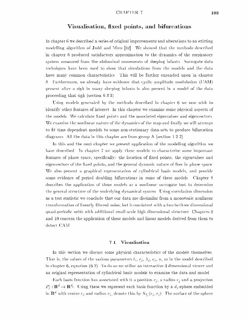
103CHAPTER 7
Visualisation, �xed points, and bifurcations
In chapter 6 we described a series of original improvements and alterations to an existing
modelling algorithm of Judd and Mees [62]. We showed that the methods described
in chapter 6 produced satisfactory approximation to the dynamics of the respiratory
system measured from the abdominal movements of sleeping infants. Surrogate data
techniques have been used to show that simulations from the models and the data
have many common characteristics. This will be further expanded upon in chapter
8. Furthermore, we already have evidence that cyclic amplitude modulation (CAM)
present after a sigh in many sleeping infants is also present in a model of the data
proceeding that sigh (section 6.3.3).
Using models generated by the methods described in chapter 6 we now wish to
identify other features of interest. In this chapter we examine some physical aspects of
the models. We calculate �xed points and the associated eigenvalues and eigenvectors.
We examine the nonlinear nature of the dynamics of the map and �nally we will attempt
to �t time dependent models to some non-stationary data sets to produce bifurcation
diagrams. All the data in this chapter are from group A (section 1.2.2).
In this and the next chapter we present application of the modelling algorithm we
have described. In chapter 7 we apply these models to characterise some important
features of phase space, speci�cally: the location of �xed points, the eigenvalues and
eigenvectors of the �xed points, and the general dynamic nature of ow in phase space.
We also present a graphical representation of cylindrical basis models, and provide
some evidence of period doubling bifurcations in some of these models. Chapter 8
describes the application of these models as a nonlinear surrogate test to determine
the general structure of the underlying dynamical system. Using correlation dimension
as a test statistic we conclude that our data are dissimilar from a monotonic nonlinear
transformation of linearly �ltered noise, but is consistent with a two to three dimensional
quasi-periodic orbit with additional small scale high dimensional structure. Chapters 9
and 10 concern the application of these models and linear models derived from them to
detect CAM.
7.1 Visualisation
In this section we discuss some physical characteristics of the models themselves.
That is, the values of the various parameters `i, rj , �j , cj , n, m in the model described
in chapter 6, equation (6.2). To do so we utilise an interactive 3 dimensional viewer and
an original representation of cylindrical basis models to examine the data and model.
Each basis function has associated with it a position cj , a radius rj and a projection
Pj : Rd 7! Rdj . Using these we represent each basis function by a dj-sphere embedded
in Rd with centre cj and radius rj , denote this by Sdj (cj; rj). The surface of the sphere

104 Chapter 7. Visualisation, �xed points, and bifurcations
Figure 7.1: Small basis functions: A three dimensional representation of the ba-
sis functions selected to model the data shown in �gure 6.1 with the modelling al-
gorithm described by Judd and Mees [62]. The spheres represent the individual ba-
sis functions. The embedding used is (yt; yt�5; yt�10). Note the small basis func-
tion on the left of the picture which would have very localised e�ect. The corre-
sponding computer �le, created with SceneViewer (VRML) is located at the URL
http://maths.uwa.edu.au/�watchman/thesis/vrml/small blobs.vrml.

7.1. Visualisation 105
Figure 7.2: Big basis functions: A three dimensional representation of a typi-
cal model created by the methods described in chapter 6. This is a model of the
same data set as �gure 7.1. The embedding strategy used is (yt; yt�1; yt�2). Note
that there are fewer and larger basis functions (speci�cally the cylinder on the right
and the large sphere to the left) than in �gure 7.1. Furthermore, these basis func-
tions represent a nonuniform embedding. Three cylinders are aligned along the
same co-ordinate axis. This represents the same embedding strategy. The corre-
sponding computer �le, created with SceneViewer (VRML) is located at the URL
http://maths.uwa.edu.au/�watchman/thesis/vrml/big blobs.vrml.

106 Chapter 7. Visualisation, �xed points, and bifurcations
is given by
Sdj (cj ; rj) =
(x 2 Rd : �j(x) = �
s2(1� %j)
%j
kPj(x� cj)k
rj
%j
2
!= 1
)
where �j is the jth basis function. We project this surface to a 3 dimensional subspace
of Rd and draw Sdj(cj ; rj) as the corresponding sphere, cylinder or prism. Furthermore,
Sdj (cj; rj) is coloured according to the value of �j . Using this representation one is able
to view a projection of the model in Rd into R3. In chapter 6, �gure 6.5 illustrates such
a representation for one model of the data illustrated in �gure 6.1.
Using these techniques we notice several interesting features of these models. Models
built using the description length criteria introduced in [62] tend to have a lot of little
basis functions covering only a small number of data points (typically 1{3). Often, these
basis functions will also exhibit extreme1 values of �j . These basis functions therefore
may only have a very local e�ect and are possibly not important to the dynamics of
the original system. They serve only to correct the model at a (very) few embedded
points. One could therefore exclude such basis functions from the model and use the
model produced only as the sum of the larger basis functions. However, this is exactly
equivalent to the harsher description length criterion introduced in section 6.2.3. Figure
7.1 shows an example of a model produced by such methods. Models produced after
implementing the improvements discussed in chapter 6 have fewer small basis functions.
A more perplexing feature of the models produced after implementing the improve-
ments of chapter 6 is that they are more likely to exhibit particularly large basis functions
| having radii several times larger than the data. These functions would certainly be
only very slightly nonlinear over the range of the data one is �tting and therefore could
be used to �t very slight nonlinearity in the model. Figure 7.2 shows an example of such
a situation. One may also note something that should be apparent by examining the
projections Pj . Very often models of a single data set will always exhibit the majority
of the basis functions aligned along a speci�c set of coordinate axes. There is an obvious
preference for some embedding strategies over others.
This preference for particular embedding strategies is a comforting and not partic-
ularly surprising consequence of the fact that some of the embedding coordinates have
a stronger e�ect on the future evolution than others [64]. Furthermore, the range of
di�erent positions and nature of basis functions is far less in the models produced by the
methods of chapter 6 than those suggested by [64]. This gives additional evidence that
the methods discussed in chapter 6 are more repeatable than the original algorithm.
1Typically the value of �j for a small basis function over a single data point will be several orders of
magnitude larger than the corresponding coe�cients of the \larger" basis functions.

7.2. Phase space 107
−2 0 2−1
−0.5
0
0.5
y−2 0 2
−1
−0.5
0
0.5
y−2 0 2
−1
−0.5
0
0.5
y
f(y,
y,...
,y)−
y
Figure 7.3: The function f(y; y; : : : ; y) for three models of a respiratory data
set: This �gure shows three plots of f(y; y; : : : ; y) � y against y for three models of
the same data set. These three plots are typical of the range of results for models of
this data set and for models of any set of respiratory data. Note that although they
exhibit a range of di�erent behaviours they all have one �xed point in the same general
location. The di�erent results elsewhere are due to the fact that the line (y; y; : : : ; y) is
generally located far from the data | in most cases the data sets we have recorded do
not tend to a �xed point.
7.2 Phase space
Given a model of the form
zt+1 = F (zt)
, (yt+1; yt; : : : ; yt�(d�2)) = (f(zt); yt; : : : ; yt�(d�2))
for the vector variable zt = (yt; yt�1; : : : ; yt�(d�1)) a fundamental property of the func-
tion F and the dynamics it produces is the values of z0 such that z0 = F (z0), the �xed
points of F . By examining the associated values of the eigenvalues and eigenvectors of
the linearisation DFz0 at z0 one may determine the local stability of F . For a discussion
of this see [47].
The �xed points of the map F will be points of the form z0 = (y0; y0; y0; : : : ; y0) such
that y0 = f(y0; y0; : : : ; y0). To �nd the �xed points of F it is simply a matter of solving
a scalar function of a single variable. Figure 7.3 gives examples of typical behaviour
of this function for models of infant respiration. For each �xed point z0 of F one may

108 Chapter 7. Visualisation, �xed points, and bifurcations
linearise about z0 and calculate the eigenvalues and eigenvectors of the derivative of F .
DzF (z)jz=z0 =
266666664
dfdy1jz=z0
dfdy2jz=z0 : : : df
dyd�1jz=z0
dfdydjz=z0
1 0 : : : 0 0
0 1 : : : 0 0...
.... . .
......
0 0 : : : 1 0
377777775
=
266666664
dfdz jz=z0
Id�1
0
0...
0
377777775
where z = (y1; y2; : : : ; yd) and Id�1 denotes the (d� 1)� (d� 1) identity matrix. The
eigenvalues �i can be calculated as the solutions of
det(DzF (z)jz=z0 � �iI) = 0; i = 1; 2; : : : ; d
and the corresponding eigenvectors from
DzF (z)jz=z0vi = �ivi:
7.2.1 Results Data from 16 healthy infants were recorded during quiet sleep on
four separate occasions at 1, 2, 4 and 6 months of age. These data are from group A
(section 1.2.2). For each of 56 data sets of respiratory movement during quiet sleep we
built a cylindrical basis model following the methods described in chapter 6. All these
models exhibited a periodic or quasi-periodic limit cycle2, and they all had at least
one �xed point. Only 10 of the models exhibited more than one �xed point. All data
sets exhibited a �xed point situated approximately in the centre of the (quasi-)periodic
orbit. The line f(y; y; : : : ; y) = y will pass through the periodic orbit. In 52 cases
the leading (largest) eigenvalue �1 of that �xed point was complex with Re (�1) < 13.
The remaining 4 models had a largest eigenvalue which was real with j�1j � 14. This
indicates that in almost all cases these models exhibit a stable focus. The 4 exceptions
also exhibited some rotational e�ect but not in the direction of the largest eigenvalue.
Whilst these results are important it must be noted that the �xed point is situated far
from the data (see �gure 7.4). Hence we should conclude that these models typically
have a stable focus situated approximately in the \centre" of the \quasi-periodic orbit"
of the data.2By quasi-periodic limit cycle we mean a quasi-periodic orbit asymptotically covering the surface of
a solid homeomorphic to a torus. That is, trajectories lie on the surface of a torus like solid and are
typically not self intersecting.3However j�1j > 1 in 51 cases4The values were �1 = �0:914; 0:859; 1:204;�1:488.

7.2. Phase space 109
Figure 7.4: A sample model: The data set and the location of the �xed point
(the small dot in the centre) of a model of that data set. The lines radiat-
ing from the �xed point represent the direction of (the real component of) the
leading eigenvectors together with the relative magnitude of the eigenvalues. A
three dimensional computer �le representation of this �gure is located at the URL
http://maths.uwa.edu.au/�watchman/thesis/vrml/fixedpts.vrml.

110 Chapter 7. Visualisation, �xed points, and bifurcations
7.3 Flow
Characterising the behaviour at the �xed points of the model F is important, but
it is also particularly di�cult. The data from which the model is built are situated
far from the �xed point. The behaviour which is of greater signi�cance, and easier
to examine5 is that near the data. A noisy periodic or quasi periodic orbit is present
in almost every model of every stationary (or \nearly stationary") data set. In this
section we present a new qualitative analysis of some features of that behaviour and
the asymptotic approach to the limit cycle of these models. The model F is a map
(discrete dynamical system). This map has been calculated to approximate the ow of
the underlying (undoubtedly) continuous dynamical system of the human respiratory
system. We use the map of the model F to approximate this ow.
Figure 7.5 shows a typical ow for a model exhibiting a periodic orbit. This is the
type of behaviour exhibited by most models of most data sets which exhibit periodic
orbits. Models exhibiting quasi-periodic orbits exhibit behaviour more similar to that
of �gure 7.6. Note that in �gure 7.5 the initially small ball of points is squashed to
a two dimensional subset of this embedding space and stretched away from the limit
cycle. Furthermore, this \stretching" is nonlinear and creates a bend in the \tail" of
the set of points.
Figure 7.6 shows an example of a more complicated behaviour. One can see that the
initial ball of points is attened stretched and bent due to the more rapid movement of
the point near the quasi-periodic orbit. The set of points is then folded and eventually
squashed down upon itself (at the top right hand corner of the illustration) in a manner
analogous to the stretching and folding of the baker's map [25]. The baker's map
f : [0; 1]� [0; 1) 7�! [0; 1]� [0; 1) can be de�ned by
f(x; y) =
((a1x;
yb1); y < b1
(a2(1� x); 1�yb2); y � b1
where a1+ a2 < 1 and b1+ b2 = 1 6. This phenomenon is also similar to the continuous
stretching and folding exhibited by the R�ossler system [113, 41]. Figure 7.7 compares
the e�ects of the maps used in �gure 7.5 and �gure 7.6.

7.3. Flow 111
Figure 7.5: Periodic model ow: Every second iteration of a small ball of points
as it approaches the limit cycle (the solid lines) of a model of the data set of �gure
6.1 (the small dots). The embedding used is (yt; yt�5; yt�10). This plot shows every
second iteration of a small ball of points from the initial state to the 24th iteration.
Note that as the ball is iterated it is squashed down onto two directions and stretched
along the limit cycle. The stretching appears initially to by away from the limit cy-
cle (indicating an unstable, and unobservable limit cycle) however the stretching is
actually along a direction which moved toward the limit cycle (see the left hand side
of the �gure). Furthermore the tail of the \comet like" shape is bent by the slower
dynamics away from the limit cycle. The corresponding computer �le is located at
http://maths.uwa.edu.au/�watchman/thesis/vrml/flow1.iv.

112 Chapter 7. Visualisation, �xed points, and bifurcations
Figure 7.6: Chaotic model ow: Every second iteration of a small ball of points as it
approaches the limit cycle (the solid lines) of a model of the data set of �gure 6.1 (the
small dots). The embedding used is (yt; yt�5; yt�10). This plot shows every second itera-
tion of a small ball of points from the initial state to the 24th iteration. Note the stretch-
ing and folding behaviour. The initial ball of points is stretched and folded to resemble
a boomerang (front, bottom, centre of the �gure) the \wings" of which are then folded
in on themselves (top, right corner of the limit cycle). The corresponding computer �le
is located at http://maths.uwa.edu.au/�watchman/thesis/vrml/flow2.iv.

7.3. Flow 113
−0.65 −0.6 −0.55 −0.5 −0.45 −0.4
−0.4−0.35
−0.3−0.25
−0.2−0.15
−0.2
0
x1x2
x3
−1.1−1.05
−1−0.95
−0.9
−1.2−1.1
−1−0.9−1.2
−1
−0.8
x1x2
x3
−1.2−1
−0.8
−1.4−1.2
−1−0.8
−0.6−1.5
−1
−0.5
x1x2
x3
Figure 7.7: Model ow: The three plots are (from top to bottom): the initial ball of
points used in �gure 7.5 and 7.6; the 24th iteration of the ball of points under the map
of �gure 7.5; and the 24th iteration of the same points under the map of �gure 7.6.
The embedding used is (yt; yt�5; yt�10). Note that the map of �gure 7.5 simply attens
stretches and bends the initial ball, the map of �gure 7.6 actually folds these points.

114 Chapter 7. Visualisation, �xed points, and bifurcations
2 2.125 2.25 2.375 2.51
1.5
2
2.5
(c)
−1.71541 −0.516798 0.681818 1.88043 3.079050
1
2
3
(b)
0 20 40 60 80 100 1200
2
4
6(a
)
2.25 2.28125 2.3125 2.34375 2.3751
1.5
2
2.5
bifurcation parameter
(d)
Figure 7.8: The bifurcation diagram: Panel (a) shows the tidal volume (the di�er-
ence between peak inspiration and expiration) of the 131 breaths that occurred during
the data set used to build the model. The data set is the same as that shown in �g-
ure 6.1. Each of panel (b), (c), and (d) show the asymptotic values of tidal volume
which occurred in free run predictions (no noise) of the model for �xed values of the
bifurcation parameter �(t). The horizontal axis is �(t). Panels (c) and (d) are enlarge-
ments of plots (b) and (c), respectively. The region of the enlargement is shown by the
dashed vertical lines. The horizontal axes in (a) is breath number, but this corresponds
to the value of �(t) shown in (b).

7.4. Bifurcation diagrams 115
7.4 Bifurcation diagrams
Models of the form discussed in chapter 6 are stationary and work under the as-
sumption that the data are stationary. However in many complex systems, including
physiological ones, this is not always the case. These models may be generalised so that
instead of
zt+1 = F (zt)
= (f(zt); yt; : : : ; yt�(d�2))
as in (7.2) one builds a new model in which time is explicitly a parameter
zt+1 = F (zt; �(t)) (7.1)
= (f(zt; �(t)); yt; : : : ; yt�(d�2)):
The nonlinear modelling algorithm one uses to �t F (actually f) to the data should
be able to model the transformation � so that one can build a model zt+1 = F (xt; t).
However, for ease of computation we apply an a�ne transformation � to t so that
�(1) = min (yt) and �(N) = max (yt). One may think of �(t) as the bifurcation parameter
of the model F and in general choose � to be a nonlinear transformation that represents
the changing behaviour of the system. It need not even be monotonic. A similar
approach has been applied by Judd and Mees [63] to model the chaotic motion of a
string and infer the presence of a Shil'nikov mechanism [41, 124, 125, 126].
This additional parameter has the e�ect of adding an extra dimension and stretching
out the data in phase space. Hence the original (quasi-)periodic orbit occupied by the
data has become a thin helix through phase space and the problems associated with
modelling it have also increased. However, in this section we build a model of the form
(7.1). The data set we use is the same as in chapter 6. It has been illustrated in �gure
6.1. From this data set we build a model with the bifurcation parameter �(t) constrained
to be a simple a�ne transformation of sample time. From this model we �xed �(�t) and
observed the asymptotic behaviour of F (�; �(�t)). The results of �gure 7.8 clearly show
that the amplitude of the limit cycle (equivalently, the Poincar�e section of F (�; �(�t)))
undergoes a period doubling bifurcation and degenerates to chaos precisely before the
sigh in this recording and the onset of apnea [65].
Repeated application of this modelling method to the same data set was unable to
produce identical results. Similar results were obtained but not with identical features
5At least in a qualitative sense. In chapter 10 we discuss a quantitative analysis of this behaviour
and the problems inherent in those approaches. Chapter 9 presents a method of linear approximation
which has lead to substantial success.6The baker's map is a two dimensional, injective variant on the tent map
f(x) =
(2x; x < 1
2
2� 2x; x � 12
However, the baker's map is discontinuous. The phenomenon we observe in �gure 7.6 is continuous.
116 Chapter 7. Visualisation, �xed points, and bifurcations
and not on every occasion. Hence, although this is an interesting and particularly ap-
pealing phenomenon we are tempted to treat it as an artifact of the modelling process,
and not representative of the data. These calculations show that such a spectacular
bifurcation o�ers an acceptable model for respiration prior to the onset of apnea. This
model exhibits qualitative and quantitative features of the data, simulations from this
model has the same features as the data. Hopf bifurcations have been o�ered by other
authors [17] as an explanation for phenomena, including periodic breathing, in respi-
ration. Unlike our models, these systems are constructed to share some qualitative
features with the data and have (by construction) the necessary bifurcation. The pe-
riod doubling bifurcation we observe in �gure 7.8 is not a consequence of the form of
model we choose to examine, it is a property of the �t of equation (7.1) to the data.
We are not programming these features into the model, we extract them from the data.
We believe that the model which produced the bifurcation diagram of �gure 7.8 o�ers
a far superior �t to this data. It shares more qualitative similarities with the data
the possible arti�cial systems. However, it is not the only acceptable explanation | in
chapter 6 we showed that models with no explicit time-dependence o�ered a satisfactory
representation of this data set.
7.5 Conclusion
In this chapter we presented a characterisation of several features of the hypothesised
generic dynamics of respiration based upon the qualitative and quantitative features
of models of respiratory data. We demonstrated a new method by which one can
visualise these complex cylindrical basis models, and using this we drew conclusion
about the modelling algorithm itself. In particular, we demonstrated that the modelling
method described by Judd and Mess [62] often over �ts the data. Some basis functions
had an e�ect on only a very few number of data points | fewer than the number of
parameters required to specify those basis functions. We demonstrated that not only
did the modelling methods described in chapter 6 avoid this but they were more able to
�t particularly large basis functions to account for subtly slight nonlinearities evident
in the data.
In section 7.2 we made some general comments about the nature of the phase space
of models of these data. In general these models will exhibit a periodic or quasi periodic
orbit and at least on �xed point. That �xed point (on the line f(y; y; : : : ; y) = y)
will lie in the \centre" of the periodic orbit and has complex eigenvalues with the
magnitude of the real part less than one (in almost all cases this occurs with the largest
eigenvalues). Hence the �xed point of this system exhibits a stable focus in at least
two directions. Using a three dimensional viewer we made a qualitative examination of
features of this (quasi-)periodic orbit and showed two typical type of behaviours. One
associated with periodic orbits, and one with chaotic quasi-periodic orbits. For models
exhibiting periodic orbits we showed the presence of stretching and twisting as points

7.5. Conclusion 117
approach the attracting set. For models which exhibit chaotic quasi-periodic orbits
this behaviour is further exaggerated, the stretching and twisting becomes stretching
and folding in a manner analogous to the baker's map. The analysis of these features
has been mainly qualitative, in chapter 9 and chapter 10 we examine some linear and
nonlinear (respectively) quantitative methods of describing features associated with
cyclic amplitude modulation (CAM).
Finally, we built a new type of cylindrical basis model, extending the methods of
chapter 6 and incorporating time as a state variable. Some of these models exhibited
complex time dependent behaviour, and in models built on data recorded immediately
before a sigh and switching to periodic breathing we demonstrated the presence of a
period doubling bifurcation leading to chaos.

118 Chapter 7. Visualisation, �xed points, and bifurcations
119CHAPTER 8
Correlation dimension estimates
This chapter describes and summarises a study of infant breathing using data analysis
techniques derived from dynamical systems theory. We apply correlation dimension
estimation techniques (section 2.2), linear surrogate tests (chapter 3), and nonlinear
surrogate tests (chapter 4) using cylindrical basis models (chapter 6) to data of infant
respiratory patterns. Such techniques have been useful for examining other complex
physiological rhythms such as heart rate, electroencephalogram, parathyroid hormone
secretion and optico-kinetic nystagmus and can distinguish variations that are random
from those that are deterministic. Section 1.1.3 is a critical discussion of recent applica-
tions of these techniques. A similar study with di�erent data was reported in [136], in
this chapter we describe a generalisation of the study reported in [140]. Some of these
methods were presented in a preliminary form in [133].
Most studies of the dynamical behaviour of biological systems have used fractal
dimension estimation to try to establish that a system's behaviour is chaotic or to
classify distinct types of behaviour by their complexity. Recent studies have suggested
that respiration in man is chaotic. If that is the case, then techniques derived from DST
should allow the dynamical structure of respiratory behaviour to be better described
thus improving our understanding of the control of breathing.
However, these earlier studies have important limitations. Most studies have used
the Grassberger and Procaccia algorithm [44, 45] for estimating fractal dimension, which
is simple and easy to implement. Unfortunately, it is now recognised [60, 107] that
this algorithm has some technical problems that can lead to misinterpretations of data
(see section 2.2). The most serious problems occur with small data sets or when the
system incorporates a substantial noise component. The study reported here employs
the estimation algorithm of Judd [60] to determine fractal dimension. This analysis
is technically more complex, but is in practice more reliable, more robust under the
restrictions of �nite data, and less prone to misinterpretation. Estimates of fractal
dimension are used in identifying the dynamical system that produced the data we have
measured.
From dimension estimations we conclude that the dynamics of breathing during
quiet sleep are consistent with a large scale, low dimensional system with a substantial
small scale, high dimensional component i.e., a periodic orbit with a few (perhaps two
or three) degrees of freedom supplemented by smaller more complex uctuations.
The nature of the low dimensional system is investigated further by constructing
surrogate data, which enabled us to test whether the dynamics were consistent with
linearly �ltered noise or a nonlinear dynamical system. When testing for nonlinear
dynamics one also needs to admit the possibility of some combination of linear and
nonlinear, deterministic and stochastic components. Our class of nonlinear dynamical
systems must also include linear systems and admit the possibility of a noise component.

120 Chapter 8. Correlation dimension estimates
The nonlinear models we use here to test for nonlinear determinism include such a
combination of linear and nonlinear, deterministic and stochastic e�ects (chapter 6).
Our results show clearly that in almost all cases, the dynamics are best described as a
low-dimensional nonlinear dynamical system being driven by a high-dimensional noise
source. In all cases where such a model is inconsistent with the data, the measured data
have strong indications of non-stationarity, that is, the breathing patterns changed
during the recording (for example, a sudden switch to periodic breathing occurred).
Following a brief introduction to the new dimension estimation algorithm, we de-
scribe the experimental methodology, including a description of our surrogate data
generation methods. Finally, we discuss the dimension calculations and the results of
the hypothesis testing using the surrogate data sets.
8.1 Methods
Using standard non-invasive inductive plethysmography techniques we obtained a
measurement proportional to the cross sectional area of the chest or abdomen, which is
a gauge of the lung volume (see section 1.2). The present study collected measurements
of the cross-sectional area of the abdomen of infants during natural sleep. The study
was approved by the Princess Margaret Hospital ethics committee.
8.1.1 Subjects Ten healthy infants were studied at 2 months of age, in the sleep
laboratory at Princess Margaret Hospital.1 Data recorded from these infants constitute
group A (section 1.2.2).
8.1.2 Data collection The experimental scheme is described in section 1.2. In
this section we make some relevant observations about the collection of data for this
study.
The 27 observations used to calculate dimension where selected based on sleep state
(quiet, stage 3� 4 sleep) and then on the basis of su�cient stationarity and a minimum
of four minutes in length. From each of these 240 seconds of stationary data (the
240 seconds which had the most stationary moving average) were used to calculate
dimension. All 27 observations used to calculate dimension are between 240 and 360
seconds, those used to identify CAM are between 400 and 1400 seconds.
In contrast to the study by Pilgram and colleagues [95], that examined breathing
in REM sleep, we have studied infants in quiet sleep. From measurements of electroen-
cephalogram, electromyogram and electrooculogram, sleep stage was determined using
standard polysomnographic criteria [7]. During quiet sleep breathing often appears rel-
atively regular. The possibly chaotic features of most interest are the small variations
1The study reported in [136] employed more data over a wider range of physiological conditions. In
that study thirteen healthy infants where studied at 1 month of age, in the sleep laboratory at Princess
Margaret Hospital. A further nine infants where studied at 2 months. Eight of the infants where studied
at both ages. Data were collected and analysed from infant in all sleep states at 2 di�erent ages. In the
study described here all calculations are performed on 2 month old infants in quiet sleep (stage 3{4).

8.2. Data analysis 121
from this regular periodic behaviour. Because we wish to observe such �ne detail we did
not �lter signals. The analogue output of the respiratory plethysmograph (operating
in its DC mode) has no built in �ltering. Filtering methods, such as linear �lters and
singular-value decomposition methods [95], can remove some features that we wish to
observe. Furthermore, �ltering (even to avoid aliasing) has been shown in some cases
to lead to erroneous identi�cation of chaos [84, 92].
8.2 Data analysis
In this study we employed three main analysis methods: correlation dimension es-
timation and surrogate data analysis. This section will provide a description of these
methods as they are applied here. The mathematical detail has been described in the
preceding chapters. First we discuss correlation dimension estimation and then we will
provide an overview of surrogate data techniques.
8.2.1 Dimension estimation For a detailed discussion of generalised fractal
dimension and estimation of correlation dimension dc see section 2.2.
The estimation algorithm used for the calculations in this chapter is described in
detail by Judd [60, 61], an alternative treatment may be found in (for example) [58].
One important advantage of the new method is that it is possible to calculate error
bars for dimension estimates. The con�dence intervals on the dimension the algorithm
provides are dependent on the length of the time series.
For each time series the dimension was calculated for time-delay embedding (see
section 2.1) in 2, 3, 4, 5, 7, and 9 dimensions. A far greater range than necessary,
but one which encompasses suitable values of embedding dimension suggested by false
nearest neighbour methods (section 2.1.1).
Hence, for each data set our dimension estimation methods produced a graph with
many lines on it. Each line on the graph is the dimension estimate for the same data set
with a di�erent embedding dimension. These lines are a plot of the change in correlation
dimension (vertical axis) with scale (horizontal). Scale is calculated as the logarithm of
\viewing scale", so moving to the right on a plot indicates increasing scale. The right
hand end of the plots is the estimate of dimension at the largest scale (the most obvious
features) whereas the left hand end is the dimension estimate at the smallest scale (the
�nest details).
8.2.2 Linear surrogates Estimating the dimension of the data set gave valuable
information about the geometric structure of that data, but dimension estimation alone
is not enough to give a sure indication of the presence of low dimensional chaos or even
nonlinear dynamics. Any experimentally obtained data will include some observational
noise and when added to a deterministic linear process, can produce dimension estimates
not dissimilar to the results of our calculations.

122 Chapter 8. Correlation dimension estimates
To determine if our results indicate the presence of anything more complicated than a
noisy linear system we employed the surrogate data methods described by Theiler [152].
Standard linear surrogate techniques were discussed at some length in chapter 3
8.2.3 Cycle shu�ed surrogates Similarly we generated surrogates according
to Theiler's cycle randomising method [151, 154] (section 3.3) to test for any temporal
correlation between cycles. Unlike epileptic electroencephalogram signals (which have
regular sharp spikes) many data sets do not have a convenient point at which to break
the cycles. It is important to separate the cycles at points which will not introduce
non-di�erentiability that is not present in the original data. For our data we split the
data at maximum and minimum value, as respiratory data have reasonably at peaks
and troughs. We also split mid inspiration (inhalation) as the gradient is fairly constant
over this part of the respiratory cycle.
To split the cycles we �rst must decide on an appropriate place to break them. Three
obvious candidates are at the peak and trough values (where the data are relatively
at) and mid inspiration (where the gradient is steep and almost constant). Figure 8.1
illustrates these three di�erent methods for a relatively regular data set (irregular data
results in more non-stationary surrogates).
8.2.4 Nonlinear surrogates For each set of data we have calculated its corre-
lation dimension. Using a slight generalisation of the modelling algorithm described in
chapter 6 we constructed a cylindrical basis model of the data. We build a model of the
form
yt+1 = f(vt) + g(vt)�t; (8.1)
where vt is a d-dimensional embedding the scalar time series yt and �t are Gaussian ran-
dom variates. Observe that by using a time-delay embedding the only new component
of vt+1 that the model needs to predict is yt+1 (for these models embedding lag � = 1).
Both f and g are distinct functions of the form
a0 +dX
i=0
biyt�i +nX
j=1
�j exp
�1� �j�j
�kPj(vt � �j)k
�j
��j�; (8.2)
where a0, bi, �j , �j and �j are scalar constants, �j are arbitrary points in Rd and Pj
are projections onto arbitrary subsets of coordinate components. Such a model is called
a pseudo-linear model with variable embedding and variance correction. For computa-
tional simplicity we set �j = 2 for all j in the function g. The precise meaning of most of
these parameters is not important, the parameters can change greatly without a�ecting
the actual behaviour of the model. Some models of the form described in chapter 6
left non-identically distributed modelling errors (section 6.4.2). These models implied
that the system exhibited state dependent noise. Models of the form 8.1 produced
simulations (noise driven free run predictions) su�ciently similar to the data.

8.2. Data analysis 123
0 500 1000 1500
−2.5
−2
data
0 500 1000 1500
−2.5
−2
Shuffled − maximum
0 500 1000 1500
−2.5
−2
Shuffled − mean value
0 500 1000 1500
−2.5
−2
Shuffled − minimum
Figure 8.1: Cycle shu�ed surrogates: Examples of cycle shu�ed surrogates and
the data used to generate them. The three surrogates have had the cycles split at the
peak, mid inspiration (upwards movement), and at the trough. Note that the data
are slightly more stationary than the surrogates. These surrogates are typical of those
generated from this data set. In many other data sets however the stationarity was more
pronounced in the surrogates whose cycles were split at the troughs. Most data sets
exhibited greatest non-stationarity in surrogates generated by splitting at the peaks.
The degree of stationarity is re ected in the correlation dimension estimates (see �gure
8.7).

124 Chapter 8. Correlation dimension estimates
The embedding parameters utilised in these models are the same as those described
in section 2.1. We build cylindrical basis models with a time delay embedding using
de = 4 and � = 14(approximate period) � (�rst zero of autocorrelation) according to
the methods described in chapter 2 and 5.
These models will typically produce free run predictions (iterated predictions with-
out noise) that exhibit periodic or almost periodic orbits. The addition of dynamic
noise will produce simulations (iterated predictions with noise) that exhibit behaviour
similar in appearance to the experimental data. Figure 8.6 gives an example of some
data generated by the methods we use. From each model we generate surrogates as
noise driven simulations of that model. Some theoretical concerns with this type of
surrogate generation was discussed in chapter 4. We demonstrated that statistics based
on the correlation integral are pivotal (proposition 4.1) provided they can be reliably
estimated. In the analysis described here we calculated the correlation dimension curve
for each set of surrogate data for each of de = 3; 4; 5.
We expect our data to be most consistent with some type of nonlinear dynamical
system. Before considering this type of surrogate it is necessary to determine if a
simpler description of the data would be su�cient. To do this we compared our data to
surrogates generated by the traditional (linear) methods (see section 3.2). Many studies
in biological sciences have employed these traditional surrogate methods (in particular
[3, 100, 118, 156, 168]). These methods determine if experimental data are signi�cantly
di�erent from speci�c (broad) categories of linear systems. In addition to these linear
surrogate tests, we applied a new more complicated nonlinear surrogate test [137, 134].
This method was used to determine if the data are distinguishable from that generated
by a broad class of nonlinear models (see section 4.1.3 and 4.3).
8.3 Results
We �rst present our results from applying our dimension estimation algorithm. Fol-
lowing this we describe the results of our surrogate data and RARM calculations.
8.3.1 Dimension estimation The results of the calculations of dc("0), as shown
in �gure 8.2, can be summarised as follows. All calculations fall into two broad cat-
egories. Most of the estimates of dc("0) produced curves that increase, more or less
linearly, with decreasing scale log "0 but some showed an initial decrease in dimension
before increasing with decreasing scale (�gure 8.2, subjects 1 and 4). For any partic-
ular data set it was generally found that the the graph of dc("0) was shifted to higher
dimensions as the embedding dimension was increased, although the shape of the graph
varied little with changes in embedding dimension. In nearly all cases the dimension
estimates at the largest scale lay between two and three.
The more or less linear increase in dimension with decreasing scale "0, and the shift
to higher dimensions as the embedding dimension is increased, are both indications

8.3. Results 125
−2.5 −2 −1.5 −1
2
2.5
3
3.5
4
4.5
Dim
ensi
on
Subject 1
−2.5 −2 −1.5 −1 −0.50
1
2
3
4
5
Dim
ensi
on
Subject 2
−2.5 −2 −1.5 −1 −0.5
1.5
2
2.5
3
3.5
4
Dim
ensi
on
Subject 3
−2.5 −2 −1.5 −1 −0.50
1
2
3
4
Dim
ensi
on
Subject 4
−2.5 −2 −1.5 −1 −0.51.5
2
2.5
3
3.5
4
Dim
ensi
on
Subject 5
−3 −2 −1
2
2.5
3
3.5
4
4.5
Dim
ensi
on
Subject 6
−2 −1.5 −1 −0.50
1
2
3
4
Dim
ensi
on
Subject 7
−2 −1.5 −1 −0.5
2
2.5
3
3.5
4
4.5
Dim
ensi
on
Subject 8
−4 −3 −22
3
4
5
6
Dim
ensi
on
Subject 9
−2.5 −2 −1.5 −1 −0.5
2
3
4
Dim
ensi
on
Subject 10
Figure 8.2: Correlation dimension estimates: Correlation dimension estimates for
one representative data set from each of the ten subjects. Any data sets that produced
dimension estimates dissimilar to those illustrated here are discussed in the text (see
section 8.3.1) The plots are of scale (log "0) against correlation dimension with con�dence
intervals shown as dotted lines (often indistinguishable from the estimate). Correlation
dimension estimates where produced for embedding dimensions of 2, 3, 4, 5, 7 and 9
for all data sets except subjects 2, 4, and 7. Subjects 4 and 7 failed to produce an
estimate for the 9 dimensional embedding. Subject 2 did not produce an estimate when
embedded in 3 or 9 dimensions. All other dimension estimates are illustrated; higher
embedding dimension produces larger correlation dimension.

126 Chapter 8. Correlation dimension estimates
−2 −1 01.5
2
2.5
3
Dimension
0 50 100 150 200
−2
0
2
4
6
time (sec)
Data
Figure 8.3: Dimension estimate for subject 8: One of the data sets used in our anal-
ysis. The periodic breathing caused the dimension estimates (the dimension estimates
used embedding dimensions of 2, 3, 4, 5, 7, and 9) at large scale to increase.
that the system, or measurements, have a substantial component of small scale high
dimensional dynamics, or noise, at small to moderate scales. The increase of dimension
with decreasing scale is an obvious e�ect of high-dimensional dynamics or noise. The
shifting to higher dimensions with increasing embedding dimension occurs because in
higher-dimensional embedding the points \move away" from their neighbours and tend
to become equidistant from each other, which in e�ect ampli�es, or propagates, the small
scale, high-dimensional properties to large scales. (This e�ect is related to the counter-
intuitive fact that spheres in higher-dimensions have most of their volume close to their
surfaces rather than near their centres as is the case in two and three dimensions.)
Some of the dimension estimates, particularly in two and three dimensions, pro-
duced curves which linearly increased for large length scales, but appeared to level o�
as length scale decreased. For most of the estimates we have computed this is the case
when the data are embedded in two dimensions. Furthermore for these embeddings
in two dimensional space the correlation dimension estimate seemed to approach two.
This indicates that as we look \closer" at the data (that is, at a smaller length scale),
it appears to �ll up all of our embedding space. For many of the dimension estimates
(�gure 8.2, subjects 7 and 9) the embedding in three dimensions also levelled at values
slightly less than three. This behaviour can be attributed to an attractor with correla-
tion dimension of approximately 2:8 to 2:9. However, it is probably more likely that this
too is simply due to the data \�lling up" the three dimensional space. This is consistent
with the results of our false nearest neighbour calculations which suggested that three
or four dimensional space would be required to successfully embed the data.
There is one particular estimate which appeared to behave quite di�erently to all the
others. Some of the curves of the estimates for subject 8 appeared to increase, decrease,

8.3. Results 127
−3 −2 −11
2
3Dimension
0 50 100 150 200−2
0
2
4
time (sec)
Data
Figure 8.4: Dimension estimate for subject 2: One of our data sets along with
the dimension estimates (shown are the estimate with an embedding dimension of 2, 3,
and 4). Note the large sighs during the recording and the corresponding increase in the
dimension estimate at moderate scale. Another data set from the same infant exhibited
similar behaviour and produced a similar dimension estimate.
and then increase again2. This could indicate that as we look closer at the structure
there is some length scale for which the embedding structure seems to be relatively
high in dimension, whilst by looking at an even small length scale the behaviour has
signi�cantly lower dimension. These observations are supported by what we can observe
directly from the data. This time series includes an episode of periodic breathing |
increasing the complexity of the large scale behaviour (see �gure 8.3). Similarly, some of
the data sets for subject 2 include large sighs causing the dimension estimate to increase
at large scales (see �gure 8.4).
Finally, the remainder of the estimates (for example �gure 8.2, subjects 1, 2 4,
6, 7, 8 and 10) behaved in yet another manner. These estimates are approximately
constant for a small range of large length scales and gradually increased over small
length scales. The estimates at large length scales were generally about two to three,
indicating that the large scale behaviour is slightly above two dimensional. The increase
in dimension estimate for smaller length scales can again be attributed to either noise
or high dimensional dynamics. However, the scale of \small scale structure" in the
dimension estimates is at a larger scale than the instrumentation noise level. Typically
the smallest scale is ln("0) � �2:5, a scale of approximately 5% of the attractor (e�3 �
0:049787 � 0:05). The digitised signal will typically use at least 10 bits of the AD
convertor (2�10 = 1=1024 < 0:001), other sources of instrumental error are certainly at
levels less that 5%.
The approximately two dimensional behaviour is probably due to the regular inspi-
2This is not the case in �gure 8.2, �gure 8.3 gives an example of this behaviour

128 Chapter 8. Correlation dimension estimates
ration/expiration cycle along with breath to breath variation within that cycle. This
is easily visualised as the orbit of a point around the surface of a torus. A dimension
estimate of two could indicate that the attractor was any two dimensional surface, the
embedded data however have an approximately toroidal or ribbon like shape (see �gures
7.5 and 7.6). In this motion there is two characteristic cycles, �rstly the motion around
the centre of the torus or ribbon, and secondly a twisting motion around the surface.
Our estimates slightly over two indicate that this behaviour is complicated further by
some other roughness over the surface of the attractor. The shape of a toroidal attractor
would very closely resemble the textured surface of a doughnut. A ribbon like attractor
would consist of some portion of the surface of this doughnut.
8.3.2 Linear surrogates Dimension estimation has given information about the
shape of the dynamical system we are studying. In an attempt to classify this system
we apply surrogate data techniques. First we compare breathing dynamics to linear
systems. Following this, we compare the breathing dynamics to nonlinear dynamical
systems by �tting a type of nonlinear model to the data.
By comparing the value of dimension obtained from our data and surrogates con-
sistent with each of these three null hypotheses we were able to reject all three null
hypotheses (see �gure 8.5 for an example of such a calculation). These results are
summarised in appendix A.
Pilgram's [95] work with respiratory traces during REM sleep produced similar ob-
servations for a di�erent physiological phenomenon. By rejecting these null hypotheses
we may make two important observations. Firstly, the data are not a (monotonic)
transformation of linearly �ltered noise. And secondly, correlation dimension alone is
su�cient to distinguish between our data and data consistent with these hypotheses.
These results, however comforting, are not particularly surprising. Our data are
regular and periodic, and the surrogates are not (see, for example �gure 8.6).
8.3.3 Cycle shu�ed surrogates The dimension estimates for cycle shu�ed
surrogates in �gure 8.7 are typical of those produced by these surrogates. In almost all
cases the dimension of the data was signi�cantly lower than that of the surrogates. For
26 of our 27 data sets data and surrogate were signi�cantly di�erent for each of these
linear hypotheses for at least one of de = 3; 4; 5. This would suggest that shu�ing the
cycles has increased the dimension of the time series, replacing deterministic behaviour
with stochastic.
Figure 8.7 shows calculation of dimension estimates for such surrogates. There is a
clear rejection of the hypothesis that there is no temporal correlation between cycles.
Shu�ing the cycles produces surrogates that are often non-stationary and are distin-
guishable from cursory examination. We are unable to reject the hypothesis that the
system is a noise driven (or chaotic) periodic orbit. In all our calculations the surrogate
dimension estimates are highest when the surrogates are most non-stationary. The most

8.3. Results 129
−2 −1.5 −1 −0.52.5
3
3.5
4Algorithm 0; 4 dimensional embedding
−2.5 −2 −1.5 −1 −0.52.5
3
3.5
4
4.5Algorithm 1; 4 dimensional embedding
−2 −1.5 −1 −0.5 02.5
3
3.5
4
4.5Algorithm 0; 5 dimensional embedding
−2 −1.5 −1 −0.52.5
3
3.5
4
4.5
5
5.5Algorithm 1; 5 dimensional embedding
−2 −1.5 −1 −0.52.5
3
3.5
4Algorithm 2; 4 dimensional embedding
−2 −1.5 −1 −0.5 02.5
3
3.5
4
4.5
5Algorithm 2; 5 dimensional embedding
Figure 8.5: Linear surrogate calculations: An example of the surrogate data calcu-
lations for algorithm 0, 1 and 2. Here we compared the correlation dimension estimate
for one of our data sets (solid line) and 30 surrogates (dotted lines). There is a clear
di�erence between the correlation dimension of the data and that of the surrogates.

130 Chapter 8. Correlation dimension estimates
0 20 40 60 80 100 120−2
0
2
4Data
0 20 40 60 80 100 120−2
0
2
4Algorithm 0
0 20 40 60 80 100 120−2
0
2
4Algorithm 1
0 20 40 60 80 100 120−2
0
2
4Algorithm 2
0 20 40 60 80 100 120−2
0
2
4Non−linear surrogate
Figure 8.6: Surrogate data: Sections of three surrogates generated by the traditional
techniques | algorithms 0, 1 and 2 and a section of a surrogate data set generated
from a cylindrical basis model. Also shown is a section of the real data used to generate
these surrogates. There are obvious similarities between the true data and the nonlinear
surrogate, whilst the other surrogates are obviously di�erent.

8.3. Results 131
−2 −1 01.5
2
2.5
3(n
orm
alis
ed)
dc
−2 −1 02
2.5
3
3.5
4
−2 −1 02
2.5
3
3.5Shuffled at peaks
−2 −1 01.5
2
2.5
3
(nor
mal
ised
) dc
−2 −1 02
2.5
3
3.5Shuffled at mid inspiration
−2 −1 02
2.5
3
3.5
4
−2 −1 01.5
2
2.5
3
(nor
mal
ised
) dc
Embedding dimension 3−2 −1 02
2.5
3
3.5
Embedding dimension 4
Shuffled at troughs
−2 −1 02
2.5
3
3.5
4
Embedding dimension 5
Figure 8.7: Dimension estimates for cycle randomised surrogates: Surrogate
data calculations for one of our data sets, embedded in R3, R4 and R5. The data set
and representative surrogates are illustrated in �gure 8.1. In each �gure the solid line
is the correlation dimension estimate for the data, whilst the dotted lines are estimates
for 30 surrogates. The cuto� scale log("0) is plotted against correlation dimension esti-
mate dc("0). Note that in each case the correlation dimension estimates are signi�cantly
higher for the surrogates | indicating an increase in complexity with cycle randomisa-
tion.

132 Chapter 8. Correlation dimension estimates
stationary surrogates appear reasonable to cursory inspection, but yield clearly distinct
dimension estimates.
8.3.4 Nonlinear surrogates For each set of data we have calculated its corre-
lation dimension. Using a modelling algorithm described in chapter 6 we constructed
a cylindrical basis model of the data. From this model we constructed 30 surrogate
data sets. The surrogates were embedded in 2, 3, and 4 dimensions, using the same
embedding strategy as the true data set. We then calculated the correlation dimension
curve for each set of surrogate data.
The results (see �gure 8.8) of these calculations fell into two very distinct categories.
For many of the data sets the surrogates very closely resembled the true dimension
estimate whilst for some others the data and the surrogates appeared to be very di�erent.
Upon a closer examination of the time series, it appears that the model failed to produce
accurate surrogates only when the data set was signi�cantly non-stationary. Although
no data set used in these calculations had an obvious drift or changed sleep state, non-
stationarity occurred with sudden change in respiratory behaviour (see, for example,
�gure 8.3). Hence, when the data was su�ciently stationary (as was the case with
24 of our 27 data sets) the modelling algorithm produced surrogate data which were
indistinguishable (according to the method of surrogate data, with respect to correlation
dimension) from the true data. Furthermore, the models exhibited a toroidal or ribbon
like attractor with small scale complex behaviour (stochastic or chaotic) consistent with
the correlation dimension estimates.
Even if both data and surrogate were stationary the dimension estimates of the
surrogates could still be di�erent from that of the data. In all these cases however
this has been found to be a problem with the level of dynamic noise introduced to the
model to generate the surrogates. By changing the noise level the dimension would also
change, e�ectively moving the dimension estimate vertically. Since, in these cases, the
shape of the dimension estimate curves were approximately the same, by altering the
noise level it was possible to produce surrogate estimates that were indistinguishable
from the data. In all cases however, the dynamic noise was substantially less than the
model's root mean square prediction error. The root mean square prediction error is
the noise level predicted by the modelling algorithm. However this is the total noise
and includes both dynamic and observational noise.
Dynamic noise and observational noise have a di�erent e�ect on the correlation
dimension estimates. Observational noise will increase the value of correlation dimension
at length scales less than and equal to the noise level. It appears from our calculations
that increasing the level of dynamic noise increases the correlation dimension estimate
equally across all length scales | e�ectively producing a vertical shift in the estimate.
Increasing dynamic noise will certainly have a greater a�ect on dc("0) for larger "0 than a
similar increase in observational noise would. Assuming one has correctly identi�ed the

8.3. Results 133
−3 −2 −11
1.2
1.4
1.6
1.8
2
2.2
−3 −2 −1
1.5
2
2.5
3
−3.5 −3 −2.5 −2 −1.51.2
1.4
1.6
1.8
2
2.2
2.4
Data set 1
−3 −2 −11
1.2
1.4
1.6
1.8
2
2.2
2 dimensional embedding−3 −2 −1
1.4
1.6
1.8
2
2.2
2.4
3 dimensional embedding
Data set 2
−3 −2 −1
1.5
2
2.5
3
4 dimensional embedding
Figure 8.8: Nonlinear surrogate dimension estimates: Surrogate data calculations
for two of our data sets, embedded in 2, 3, and 4 dimensions. The �rst set indicated a
close agreement between data and surrogate. The second set of calculations indicated
very clear distinction. Hence the model of the �rst data set is indistinguishable (ac-
cording to correlation dimension) from a noise driven periodic orbit, whilst the model
of the second fails to produce particularly strong similarities. Notice that for almost
any value of "0, comparison of the value of dc("0) of the data and the surrogates would
also lead to these conclusions.
134 Chapter 8. Correlation dimension estimates
underlying deterministic dynamics, it may be possible to \tune" the level of dynamic
noise so that surrogates and data have approximately the same value of correlation
dimension estimates at moderate to large length scales, and then alter the level of
observational noise to tune the dimension estimates at small length scales. Hence, the
level of noise required to be unable to reject the surrogate data is an indication of
the relative proportion of dynamic and observational noise in the system. That is,
we can distinguish between random behaviour within the system (dynamic noise) and
experimental error (observational noise).
8.4 Discussion
This study has con�rmed that apparently regular breathing during quiet sleep is
possibly chaotic. This conclusion should be quali�ed. Rapp [107] observation that to
conclude that a phenomenon is chaotic is both di�cult and often irrelevant is par-
ticularly signi�cant here. In real data sets noise contamination will always increase
the dimensional complexity of the data and almost any experimental data will exhibit
non-integer correlation dimension. Identi�cation of apparently chaotic behaviour is,
however, a good �rst step in dynamical analysis. We have extended our observations
and analyses to describe the dynamical structure of the system in greater detail.
Our dimension estimate results indicate that on a large scale there is low dimensional
behaviour while the small scale behaviour was often dominated by very high dimensional
dynamics or noise (that is, extremely high dimensional dynamics). Even though false
nearest neighbour techniques suggest that we were embedding in high enough dimen-
sions, there was still some small scale behaviour which �lled the embedding space. The
scale at which the embedding space is �lled by the dynamics could indicate level of
experimental noise.
The most conclusive estimates from this study indicated that the structure of the
attractor is likely to be similar to a torus or twisted ribbon with small scale, very high
dimensional dynamics. Hence at large length scales the structure looked like the surface
of a torus or ribbon whilst at smaller length scales dimension increased. This indicates
that the attractor appears to be a torus with a very rough surface. The most important
conclusion from these data is that this two dimensional, periodic system indicates two
levels of periodicity. Hence, in addition to the periodic inspiration/expiration motion it
is likely that there was some cyclic breath to breath variation.
By applying the method of surrogate data we demonstrated that the correlation
dimension is related to the data from which we estimate it in a nontrivial way. The
surrogates produced by algorithms 0, 1, and 2 are clearly inadequate. It is apparent
that they should fail and this was con�rmed by our results. These simple surrogates
con�rm that our data are not generated by linearly �ltered noise. Similarly the sur-
rogates produced by shu�ing the cycles are di�erent from the data. This produces a
more substantial result; there is signi�cant temporal correlation between cycles. We

8.4. Discussion 135
have constructed our own surrogates using a nonlinear modelling process and compared
surrogates and data to test the accuracy of the model. For 24 of 27 data sets we found
that the data and nonlinear surrogates were indistinguishable according to correlation
dimension. For those data sets that were distinguishable from their surrogates, we found
that there were several possible reasons for this. Usually, if the data was non-stationary
the model simply failed to produce surrogates that were close enough to the data. The
model is stationary and periodic, whilst the data is not.
Occasionally, with non-stationary data the model failed to produce even periodic
surrogates. If this was the case then the model had a stable �xed point. In these cases
the dimension estimates of data and surrogate were obviously di�erent and a better
model is required. The fact that this modelling algorithm failed in cases where the
data were not stationary is not particularly surprising | both modelling and dimension
estimation algorithms require stationarity. Perhaps with improved modelling techniques
similar results could be obtained in these cases.
In conclusion, the results of this chapter address the limitations of previous studies
that have examined whether respiration is chaotic. We investigated children in quiet
sleep when breathing appears most regular. Correlation dimension estimates are con-
sistent with a chaotic system. Furthermore, unlike most previous studies, we used
surrogate data analyses to test whether the apparently chaotic behaviour was due to
linearly �ltered noise. We found this unlikely and concluded that the simplest system
consistent with our data is a noise driven nonlinear cylindrical basis model. Our data are
the most convincing evidence that respiratory variability in infants is deterministic and
not random, due to noise. A recent study has demonstrated reduced variability of res-
piratory movements in infants who subsequently died of sudden infant death syndrome
(Schechtman [119]). This observation was retrospective but suggests that because the
variability that we have observed during quiet breathing is deterministic, then further
study using dynamical systems theory could allow early identi�cation of infants at risk
of SIDS from simple measurements of respiratory patterns.

136 Chapter 8. Correlation dimension estimates
137CHAPTER 9
Reduced autoregressive modelling
Chapter 8 demonstrates the possible existence of multiple oscillators within the respi-
ratory system. In this chapter we utilise new linear modelling techniques which are an
adaption of the nonlinear techniques of chapter 6 to detect cyclic amplitude modulation
(CAM). Cyclic amplitude modulation is evidence of a second oscillator within the res-
piratory system. In chapter 10 we will discuss some more general nonlinear techniques
that can be used to detect CAM type behaviour.
9.1 Introduction
Periodic breathing is a familiar phenomenon that is not di�cult to observe. It
is characterised by periodic increases and decreases in tidal volume. Furthermore, the
period of this periodic behaviour can be easily measured and remains relatively constant
(see section 1.1.2, �gure 1.2). During quiet sleep, however, it is often possible to observe
that successive breaths uctuate almost periodically, in a way reminiscent of periodic
breathing, but not nearly as pronounced and certainly not periodically apneaic (see
�gure 1.2 prior to the onset of periodic breathing). This phenomenon we will call cyclic
amplitude modulation (CAM).
The method we employ here extends the traditional autoregressive model of order n
(AR(n)) which predicts the next value in a time series as a weighted average of the last
n values. We consider instead a reduced autoregressive model (RARM) where any past
values may be used to predict the upcoming value, but only those that are important are
used. To determine which past values are important we employed Rissanen's minimum
description length (MDL) criterion [110] (see section 2.3.2), using a modelling procedure
originally described by Judd and Mees [62, 64]. In chapter 2 and 6 we outline this
modelling procedure in the context of nonlinear radial (cylindrical) basis models our
implementation of these methods for linear modelling has been presented elsewhere [133]
(abstract), and will be discussed in future work [138]. A description of the mathematical
methods is presented in a nonlinear context in section 2.3.3 and a linear application will
be described in section 9.4. For now let us assume that RARM can produce a model
consisting only of those previous values that are useful in predicting future values. This
is not necessarily a particularly good model in terms of prediction | it is only an
approximation to the breath to breath dynamics which we utilise to extract important
information. We built reduced autoregressive models of tidal time series extracted
from the original data. Successive elements of this tidal time series correspond to
the magnitude of successive breaths. Using this information we deduce the period of
approximately periodic behaviour in the time series from the temporal separation of
the previous values. Hence RARM can identify the period of CAM in much the same
way as autocorrelation may, except our methods prove to be more sensitive and more
discriminatory.

138 Chapter 9. Reduced autoregressive modelling
By reducing the original data to a breath to breath time series we e�ectively rescale
the time axes so that each breath is of equal length. However, CAM on a breath to breath
basis does not (necessarily) suppress time dependent dynamics. A hypothesised cyclic
variation in breath duration may be related to a cyclic variation in breath amplitude
(and hence evident in the breath amplitude time series). These could essentially be two
separate observations of the same periodic behaviour. The \duration" of a single breath
is also far more di�cult to measure accurately due to (relatively) long at peaks and
troughs.
Other authors (see for example [11, 160]) have attempted to identify cyclic behaviour
in breath sizes. Unlike previous methods which require careful measurement of respira-
tory parameters from a strip chart, our method is purely quantitative and completely
automated. Furthermore, our method is applied to time series for which there is no
obvious cyclic amplitude modulation. We will show that RARM algorithm can identify
CAM when other methods, such as spectral analysis and estimates of autocorrelation
do not.
Fleming and others [34] have demonstrated cyclic oscillations in infants under 48
hours old during quiet sleep and after a sigh. In older infants the observed a decrease
in this phenomenon.
Some time ago Waggener and colleagues [12, 160] observed cyclic variation in high
altitude ventilatory patterns of adult humans. They identi�ed the period of cyclic
variation by inspection of the strip chart and drew most of their conclusions from
variation in the strength of the ventilatory oscillation. In [12] and another series of
studies, Waggener and colleagues applied a comb �lter [11] to detect periodicities. A
comb �lter is a series of band pass �lters, which, e�ectively act as a coarse approximation
to the Fourier spectrum. Using this technique they demonstrated apparent ventilatory
oscillations preceding apnea [162] and a link between apnea duration and ventilatory
oscillations [164, 161]. However, no link between periodic oscillations (detected using a
comb �lter) and sudden infant death [163] was found.
More recently Schechtman and others [119] identi�ed signi�cant di�erences in the
�rst return plot of inter-breath times of sudden infant death syndrome (SIDS) vic-
tims and normal infants. Despite dramatically under-sampled data Schechtman demon-
strated signi�cant breath to breath variation.
This chapter deals with the application of linear modelling techniques to detect and
measure CAM. We introduce a new mathematical method of detecting periodicities
based upon autoregressive modelling and the information theoretic work of Rissanen
[110]. We compare this technique to the traditional autoregressive models and tradi-
tional methods of autocorrelation and spectral analysis. The data used in this study
was collected at Princess Margaret Hospital for Children, the experimental protocol is
described in section 1.2.
9.2. Tidal volume 139
9.2 Tidal volume
In this section we will outline our data and pre-processing methods. In sections 9.3
and 9.4 we describe our mathematical techniques, and in section 9.5 we present some
experimental results.
9.2.1 Subjects Using standard non-invasive inductance plethysmography tech-
niques (section 1.2) we obtained a measurement proportional to the cross sectional area
of the chest or abdomen, which is a gauge of the lung volume. The present study col-
lected measurements of the cross-sectional area of the abdomen of infants during natural
sleep.
From the data described in section 1.2.2 we examine 31 infants, studied at ages
between 1 and 12 months. Seventeen of these infants where healthy (exhibited normal
polysomnogram) and had been volunteered for this study. These infants are from group
A. Fourteen children aged between 1 and 12 months, whom had been admitted to
Princess Margaret Hospital for an overnight sleep study, were also studied. Eight of
these subjects had been admitted to the hospital for clinical apnea, these are from the
group B data. The remaining �ve infants su�ered from bronchopulmonary dysplasia
(BPD), these are from group C.
9.2.2 Pre-processing The recorded time series represents the respiratory pat-
tern and from this we derived new time series, the successive elements of which represent
the depth of successive breaths.
To generate this time series we �rst identi�ed the value and location of the peaks
and troughs in this time series. That is, peak inspiration and peak expiration (see �gure
9.1). The peak and trough values were located by taking the most extreme value of
the time series in a sliding window. Having selected the extremum from the time series
it is possible to perform a quadratic or cubic spline interpolation. However, from our
calculation this did not change the results signi�cantly.
From these time series of local extremum we determined the size of a given breath
by calculating the di�erence between the magnitude of each peak and the following
trough. This di�erence represents the total change in the cross sectional area over one
exhalation. Hence, successive elements of this time series represent the tidal volume
of successive breaths. Since inductance plethysmography measures cross sectional area,
this new time series is actually \proportional" to change in the cross sectional area (and
not lung volume). This \proportionality" is not constant. The undeveloped rib cage of
infants is soft, and the relationship between abdominal area and lung volume may change
with sleep state, sleep position and respiratory e�ort. Furthermore it is not uncommon
for infants to undergo paradoxical breathing, that is the rib and abdomen act 180 degrees
out of phase. During data collection both rib and abdominal volume as well as air ow

140 Chapter 9. Reduced autoregressive modelling
770 780 790 800 810 820 830 840 850 860 870
−4
−2
0
2
4
6
8
time (seconds)
Bs2t8
770 780 790 800 810 820 830 840 850 860 870
−4
−2
0
2
4
6
8
time (seconds)
Peak and trough values
480 490 500 510 520 530 5400
2
4
6
8
breath number
Breath size (peak value − trough value)
Figure 9.1: Derivation of the tidal volume time series: The circles are the points
identi�ed as peak inspiration and peak expiration. The second plot shows the peak
and trough values as a function of time. It is from this that we extracted the tidal
volume series | illustrated in the third graph. The horizontal axes in the third panel is
the index of the breath size, whilst the other two panels are time: hence there is some
horizontal shift between the second and third panel. This time series shows a section of
irregular breathing and is not indicative of the data used in this study. It is used here
for illustrative purposes.

9.3. Autoregressive modelling 141
through the mouth and nose (recorded with nasal and oral thermistors1) was recorded.
From these it is possible to determine when paradoxical breathing occurred, all the
recordings in this study occurred when rib and abdominal movement were in phase.
Furthermore, EEG, EMG and EOG measurements were used to determine sleep state.
The position of an infant remained constant during each recording. For the purposes of
this study change in abdominal volume was used as an adequate representation of lung
volume. An increase in lung volume will cause an increase in cross sectional area so
that any periodic change in lung volume will cause a periodic change in cross sectional
area. All analysis is of this derived \tidal volume" time series.
In section 9.3 we apply standard autoregressive modelling techniques to detect CAM.
However, surrogate tests will show that these methods are unreliable. Furthermore, this
method is unable to estimate the period of CAM. In section 9.4 we describe the new
RARM technique and section 9.5 describes some results from this method.
9.3 Autoregressive modelling
For a scalar time series y1; y2; : : : ; yt one may apply a time delay embedding and
assume a simple two dimensional model for the dynamics"yt+1
yt
#= f
"yt
yt�1
#:
Linearising f about the �xed point (y0; y0) (where y0 = f(y0; y0)) we get that"yt+1
yn
#=
"a b
1 0
#"yt
yt�1
#+
"c
0
#; (9.1)
were a = @f@x j(x;y)=(y0 ;y0), b =
@f@y j(x;y)=(y0;y0), and c = (1 � a � b)y0. One can con�rm
that the �xed point of (9.1) occurs at ( c1�(a+b) ;
c1�(a+b))
T . Furthermore the eigenvalues
of (9.1) are given by
�1;2 = 12
�a�
pa2 + 4b
�; (9.2)
and hence the stability of (9.1) is dependent on the value of (a2 + 4b) | see �gure
9.2. By �tting a model (9.1) to a scalar time series and examining the value of the
parameters a and b one would hope to be able to infer the nature of the dynamics in the
original time-series | i.e. if there exist periodic behaviour in the original time-series.
In this section we perform some calculations to determine the reliability of estimates
of a and b from a data set and conclude that this method has limited practical use for
noisy data such as ours. However, these results do provide some evidence supporting
CAM and motivate a closer examination of this phenomenon.
1A temperature sensitive electrode. Since exhaled air is warmer than room temperature this device
give an indication of air ow.

142 Chapter 9. Reduced autoregressive modelling
UFUF
2
b = 1-a
a
b
b = 1+a
SFSF
a=2a=-2
(2,-1)(-2,-1)
a = -4b
SN
SNSN
S S
UNUN
SN
Figure 9.2: Stability diagram for equation (9.1): A plot in (a; b) space of the
stability of the �xed point of (9.1). The notation SN, UN, S, SF, UF denote regions
were the �xed point exhibits a stable node, unstable node, saddle, stable focus and
unstable focus respectively. The diagram is symmetric about the b-axis. Evidently if
a2 + 4b < 0 then the �xed point exhibits a focus. This focus is stable if jaj < 2.

9.4. Reduced autoregressive modelling 143
9.3.1 Estimation of (a; b) Writing the eigenvalues (9.2) of the �xed points of
equation (9.1) as � � i! one may ask how reliable are the estimates of � and ! from
a data set. It is useful to compare the estimates of �1;2 (or simply the discriminant
a2 + 4b) for data sets to algorithm 0 surrogates. Algorithm 1 and 2 surrogates do
not produce signi�cant results2 however, if the results of estimates of a and b for data
are indistinguishable from algorithm 0 surrogates then this would indicate that our
estimates of a and b are not signi�cant. Figure 9.3 shows the distribution of values of
(a2 + 4b) and b for algorithm 0 surrogates and a sample of 51 data sets derived from
over 10 minutes of respiratory data recorded in the usual way. Data for this analysis is
from all the groupings described in section 1.2.2.
The results of �gure 9.3 show that in the majority of data sets the estimates of
a2 + 4b and a2 are indistinguishable from estimates of these quantities for i.i.d. noise.
Hence, although the values of a2 + 4b and a2 for the data may suggest the presence
of a stable focus these statistics would yield similar results if applied to i.i.d. noise.
Furthermore, the variance of estimates of a2 + 4b and a2 is great, and therefore we
require more satisfactory techniques of detecting CAM.
9.4 Reduced autoregressive modelling
The essence of the new modelling method is to �rst accurately and e�ciently express
the tidal volume of the current breath as a linear combination (weighted average) of the
tidal volumes of preceding breaths (on average). The best way to imagine this �rst step
is that the more preceding breaths one uses in a weighted average the more accurate
the expression | but this is not e�cient. To achieve e�ciency one would select fewer
preceding breaths that more strongly in uence the present breath; this might be the
immediately preceding breaths, but might also mean a breath 9 or 10 breaths ago if there
were a strong periodicity. We use new mathematical methods drawn from information
theory to determine which preceding breaths are most strongly in uencing the current
breath. It is then a simple matter to look at the selected breaths to see periodicities.
We deduce approximately periodic behaviour in the time series by identifying a
strong similarity between the present breath size and previous breaths. If the present
breath is most similar to those immediately preceding it we cannot deduce the presence
of any periodic behaviour. However, if we can identify a signi�cant similarity between
this breath and one further in the past we can deduce the presence of some periodic
behaviour in the data. In the same way we can use the autocorrelation function to
detect periodic behaviour by observing a strong positive correlation between breaths.
Although the Fourier spectral estimate is often used to identify periodic behaviour
it is inappropriate to use this method for our data. Spectral estimation is good at
2Algorithm 1 and 2 surrogates address the hypothesis that the system is linearly �ltered noise, in
�tting the model (9.1) one assumes that the data are linearly �ltered noise.

144 Chapter 9. Reduced autoregressive modelling
0 1 2 3 4 50
2
4
6
8
10a/2
standard deviations0 1 2 3 4 5
0
2
4
6
8
10a2+4b
standard deviations
Figure 9.3: Surrogate data comparison of the estimates of (a2+4b) and a2 from
data to algorithm 0 surrogates: 51 data sets of tidal volume derived from respira-
tory recordings were used to estimate (a2+4b) and a2 . The value of these estimates was
compared to algorithm 0 surrogates and the number of standard deviations between the
two recorded. That is, for each data set we estimated (a2 + 4b) and a2 and calculated
estimates of (a2+4b) and a2 for algorithm 0 surrogates (data with the same rank distribu-
tion but no temporal correlation). Shown are plots of the distribution of the number of
standard deviation between the value of these statistics for data and surrogates. Clearly
the majority of these data sets are indistinguishable from noise. This demonstrates that
the estimates of (a2+4b) and a2 that we obtained from data are indistinct from estimates
we would be likely to obtain from i.i.d. (independent and identically distributed) noise.
Hence we cannot make any conclusion concerning dynamic correlations from estimates
of (a2 + 4b) and a2 .

9.4. Reduced autoregressive modelling 145
identifying moderately high frequency behaviour, the periodicities we expect to identify
are comparatively long period.
To describe the reduced autoregressive modelling (RARM) algorithm we will �rst
discuss linear modelling. Following this we will describe an adaptation of the description
length criteria of section 2.3.2 for linear models and our implementation of a model
selection algorithm.
9.4.1 Autoregressive models The traditional autoregressive model of order n
(an AR(n) model) attempts to model a time series fytgNt=1 by �nding the constants
a1; a2; a3; : : : ; an such that
yt = a1yt�1 + a2yt�2 + a3yt�3 + : : :+ anyt�n + et 8 t = n + 1; n+ 2; : : : ; N: (9.3)
where et is the model error. Methods for dealing with such models are well known
[104, 155].
However, a time series exhibiting periodic behaviour with period � would have strong
dependence of yt on yt�� . Hence, by building an AR(n) model and determining which
parameters are most signi�cant it may be possible to estimate the period of some peri-
odic behaviour or, more signi�cantly, several di�erent periods within the same series.
Deciding which parameters are most \signi�cant" requires sophisticated methods.
To do so just on the basis of the size of the coe�cients ai; i = 1; 2; 3; : : : ; n will rarely
be useful. We discuss the selection problem in section 9.4.2.
We wish to �t the best model to the data. A traditional AR(n) model has n param-
eters but it may be the case that only some of these are necessary. Essentially then we
are looking to �nd the best model of the form
yt = a`1yt�`1 + a`2yt�`2 + a`3yt�`3 + : : :+ a`kyt�`k + et i = n+ 1; n+ 2; : : : ; N:
where,
1 � `1 < `2 < `3 < : : : < `k � n: `i 2 Z+ 8i 2 f1; 2; 3; : : : ; kg:
That is, we only consider those parameters from equation (9.3) that are \signi�cant",
all others we set to zero. Since the data we consider does not have zero mean we will
also allow for the possible selection of a constant term. For clarity we will also relabel
the coe�cients and consider the model
yt =
8><>:
a1yt�`1 + a2yt�`2 + a3yt�`3 + : : :+ akyt�`k + et;
or
a0 + a1yt�`1 + a2yt�`2 + a3yt�`3 + : : :+ akyt�`k + et:
(9.4)
for t = n+ 1; n+ 2; : : : ; N , where,
1 � `1 < `2 < `3 < : : : < `k � n: `i 2 Z+ 8i 2 f1; 2; 3; : : : ; kg:

146 Chapter 9. Reduced autoregressive modelling
as before. The utility of setting some of the parameters to zero is that we are not over
�tting the data. If n� k then an AR(n) (or even an AR(`k)) model will have far more
parameters than necessary, many of which will be �tted to the noise of the system. Note
that the coe�cients ai estimated in (9.4) are distinct from the corresponding coe�cients
in (9.3). Some coe�cients of (9.3) are set to zero to obtain (9.4) but those remaining
coe�cients in (9.4) must be reestimated. Indeed the value of these parameters will
change upon reduction of the model (9.3) to a model of the form (9.4). To achieve this in
a consistent and meaningful way it is necessary to test the signi�cance of all parameters
and determine which terms are not signi�cant, and therefore which coe�cients may be
set to zero.
Using the concept of description length (section 2.3.2) we have a method of deciding
which parameters o�er a substantial improvement to the model. Rissanen's description
length is just one way to compare the size of a model to its accuracy, other methods
include the Schwarz [122] and Akaike [4] information criteria. Methods based on other
measures of \signi�cance" have been proposed by other authors, see for example [48]
and the citations therein.
9.4.2 Description length Roughly speaking the description length of a particu-
lar model of a time series is proportional to the number of bytes of information required
to reconstruct the original time series3. That is, the compression of the data gained
by describing the model parameters (a0; a1; a2; : : :ak ; `1; `2; : : : ; `k; k) and the modelling
prediction error (fetgNt=1). We discussed an application of description length to radial
basis modelling in section 2.3.2.
Obviously if the time series does not suit the class of models being considered then
the most economical way to do this would be to simply transmit the data. If however,
there is a model that �ts the data well then it is better to describe the model to the
receiver in addition to the (minor) deviations of the time series from that predicted from
the model. Thus description length o�ers a way to tell which model is most e�ective.
Our encoding of description length is identical to that outlined by Judd [62] and follows
the ideas described by Rissanen [110]. For a model of the form (9.4) the description
length will be given by (2.13),
L(zj�̂) + (12 + ln )k�kX
j=1
ln �̂j :
The precisions �j satisfy (2.12) (Q�)j = 1=�j where
Q = D��L(aj�̂)
= D��
�� ln
�1
(2��2)n=2e��
T �=2�2��
3To within some arbitrary (possibly the machine) precision.

9.4. Reduced autoregressive modelling 147
= D��
�n
2+
n
2ln
�2�
�T �
n
��=
n
2D�� ln
�(�BVB � y)T (�BVB � y)
�=
�nV TB VB
(�BVB � y)T (�BVB � y)
can be easily calculated.
9.4.3 Analysis We apply this new mathematical modelling technique to identify
any approximately periodic behaviour present in the time series of breath size. To
determine which model is best we apply the model selection algorithm of Judd [62] to
the trivial case | the case in which only linear models are required. This algorithm
was discussed in section 2.3.3 and it is exactly this algorithm we apply here. The set
fVigmi=1 of candidate basis functions is constrained to contain only the linear terms. If
y = (ym+1; : : : ; yN)T ;
V0 = (1; 1; : : : ; 1)T ;
V1 = (ym; : : : ; yN�1)T ;
V2 = (ym�1; : : : ; yN�2)T ;
...
Vj = (ym�j+1; : : : ; yN�j)T ;
...
Vm = (y1; : : : ; yN�m)T :
then we build the best model y =P
i �iV`i + �, subject to minimising �T � and select the
model which minimises the description length (2.13).
This new method is similar to identifying the extremum of the autocorrelation func-
tion. However, it is more sensitive and discriminatory. Our modelling method implicitly
requires a parameter m, a maximum number of past values. To overcome this we ex-
amine the models produced for a variety of di�erent maximum model sizes m (number
of past values). The RARM procedure will produce a (possibly changing) indication of
period as a function of maximum model size. We then look for the stage at which the
previous breaths used to predict the next does not change by increasing the maximum
model size. From this we deduce the period of any periodic behaviour. Figure 9.4 gives
an illustration of such a calculation. From each such illustration we can list the periods
detected along with the number of occurrences of each period. Using this information
we deduce the period of any periodic behaviour present. From the calculations displayed
in �gure 9.4, for example, we can conclude that periodic behaviour exist over 5, 9 and
12 breaths. We can infer that the breathing is approximately periodic, with period

148 Chapter 9. Reduced autoregressive modelling
0 20 40 600
5
10
15
model size
para
met
ers
RARM algorithm
111111111111111111111111111111111111111111111111111111111111222
222222222222222222222222222222222222222222222222222222223
333
33333333333333333333333333333333333333333333333333333
4 4
444
444444444444444444444444444444444444444444444444
4
5
55555555555555555555555555555555555555555555555555
5
0 0.5 10
5
frequency (/breaths)
Spectral estimate
0 10 20 30 400
0.5
1
lag
Autocorrelation
Figure 9.4: Reduced autoregressive modelling algorithm: Results of a calculation
to detect periodic behaviour. The numbers indicate the order in which the parameters
are selected, hence they are an indication of the relative importance of the parameters.
Also shown is an estimate of the autocorrelation function and a spectral estimate using
a 256 point overlapping (with 128 point overlap) Hanning window. Note the peak in the
spectral estimate at approximately 0:35 breaths�1 this corresponds to periodicity over
2.8 breaths. The more important detail | over 5, 9 and 12 breaths according to the
RAR model | is not evident in the spectral estimate. Periodic behaviour with period
5, 9 and 12 corresponds to a frequency of approximately 0:2, 0:11 and 0:083 breaths�1.
The autocorrelation function does, however have a peak at about 5 breaths and smaller
peaks at 9 and 12 breaths. These peaks are not very pronounced and would be much
harder to detect without the RARM results. This data set was selected as an example
because the autocorrelation and the spectral estimate both have pronounced peaks. It
is not representative of all our data sets: the spectral estimate and autocorrelation of
most data sets have no pronounced peaks.
12. The presence of periodic behaviour over 5 and 9 breaths does not contradict this
conclusion. These periods may represent sub-harmonics of the CAM, or (more likely)
signi�cant structure within the periodic waveform.
9.4.4 Data processing For each of the data sets we used the RARM technique
to determine the previous breath that most strongly in uences the current breath. We
built RAR models for maximum model size ranging from 1 to 60. From these models we
identi�ed any long period time dependence within the data set, and deduce the likely
period of approximately periodic behaviour.
The autocorrelation function was also calculated and the extremum of this function
are compared to the periodic behaviour detected by the RARM algorithm. Fourier
spectral estimates proved to be of no help detecting these periodicities. To test the

9.5. Experimental results 149
signi�cance of our results we applied three surrogate data tests (see chapter 3). For each
data set we built 30 surrogates of each of the three linear types described by Theiler [152]
(algorithm 0, 1, and 2) and applied our RARM algorithm to them. Applying algorithm
0 type surrogates is analogous to applying Theiler [151] cycle shu�ed surrogates to
the original time series (see section 3.3). Both surrogate generation algorithm destroy
temporal correlation over more than one breath. The tidal volume time series removes
a great deal of further information of the dynamics within a breath.
9.5 Experimental results
In the following section we describe our results with RARM. We compare our RARM
algorithm to the traditional autocorrelation function. We also verify our results using
surrogate data calculations. We then use our algorithm to determine the existence of
CAM during quiet (stage 3{4) sleep in 58 data sets from 27 infants. Following this we
applied our RARM method to 102 data sets from 31 infants (irrespective of sleep state)
and examine the relationship between CAM and apnea, and the nature of CAM before
the onset of apnea. Data used in this study are from all groups described in section
1.2.2. A comparison of the results for groups A, B, and C is described latter in this
section.
9.5.1 CAM detected using RARM In this section we present some prelimi-
nary results of the detection of CAM in the respiratory traces of infants in quiet sleep.
The data used for these calculations are di�erent from that for which the correlation
dimension was calculated in chapter 8. The data requirements of this algorithm are mod-
erately large (typically 10 minutes of recording), calculation of correlation dimension
and radial (cylindrical) basis models for such data sets proved prohibitive. Moreover,
the two types of models are entirely distinct: RARM is more robust to non-stationarity
while cylindrical basis models are better at capturing qualitative (and many quantita-
tive) features of respiration.
Table 9.1 outlines the results of our calculations applied to 14 data sets from 14
infants. Data used for these calculations were recorded during quiet sleep. Subjects
1-10 are the same subjects as used for correlation dimension estimates of chapter 8.
Data for subjects 1-6 were recorded during the same study as those used for dimension
estimates. Data for subjects 7-12 were recorded at 4 months of age, for subjects 13-14
at six months. Respiratory rate is the average respiratory rate over the duration of the
recording. Note that although there was some variability both in the respiratory rate
and the period expressed as a number of breaths, the period in seconds is relatively
constant. In most cases this period also falls within the range of periodic breathing.
In subject 11 periodic breathing with cycle times from 13:5 to 15:5 seconds occurred
during the same study.

150 Chapter 9. Reduced autoregressive modelling
subject age respiratory CAM
(months) rate (bpm) (breaths) (seconds)
1 2 20 5 15
2 2 37 9 15
3 2 24 none none
4 2 26 5 11
5 2 48 9 11
6 3 27 none none
7 4 25 7 17
8 4 32 none none
9 4 22 6 17
10 4 22 36 97
11 4 24 5 13
12 4 23 none none
13 6 22 5 14
14 6 21 9 26
Table 9.1: Detection of CAM using RARM: The CAM detected by RARM for 14
data sets. The values are shown both in time and number of breaths.
9.5.2 RAR modelling results For each time series of breath size we computed
autocorrelation and Fourier spectral estimates. We applied our RARM algorithm to
each data set and compared this to the result of applying traditional techniques. From
this we obtained the following results.
The period of periodic behaviour detected by the RAR algorithm is consistent with
the periods detected by autocorrelation. That is, if RARM detects periodic behaviour,
then it is of the same period as that detected by the autocorrelation estimate, if the
autocorrelation detects periodic behaviour at all. Furthermore, if the RARM does
not detect periodic behaviour, then neither does the autocorrelation estimate. Fourier
spectral estimates was not able to detect CAM of a period greater than about three.
The traditional techniques will often fail to detect periodic behaviour when the RARM
algorithm does detect it.
Furthermore, whenever periodic breathing, or visually obvious CAM respiratory
motion occurred the period of this behaviour agrees with the period predicted by the
RARM algorithm and by the traditional techniques, if the spectral estimation or auto-
correlation techniques detect anything. The results of the RARM process almost always
agree with one of the largest extremum of the autocorrelation function. However tradi-
tional techniques alone rarely indicate a clear periodicity.
Detection of periodic behaviour with our RARM algorithm is an indication of CAM.
In our data CAM was detected by RARM in 49 of our 102 datasets (28 of 58 in quiet

9.5. Experimental results 151
A: Volunteers
Subject Data Length Age Resp. Apnea CAM
set (seconds) Rate. (bpm) (breaths) (seconds)
subjectA As4t1 693 6 24.19 no 15 37
subjectA As4t2 2402 6 20.41 yes 10 26 29 76
subjectBb Bs2t8 951 2 37.97 yes 5 28 8 45
subjectBb Bs3t5 489 4 23.81 no 15 38
subjectG Gs3t3 1647 4 29.41 no 9 18
subjectJ Js3t4 916 4 47.62 yes 9 11
subjectJ Js4t4 1122 6 32.26 yes 34 6 63 11
subjectL Ls3t2 1174 4 34.09 no 6 8 11 14
subjectM Ms3t3 1700 4 27.03 yes 7 27 16 60
subjectN Ns3t4 509 4 26.79 no 23 52
subjectR Rs2t4 1357 2 35.71 yes 8 13
Table 9.2: continued on next page.
sleep). The period of the CAM detected by RARM in quiet sleep is summarised in table
9.2. The respiratory rate given in this table is the average rate of respiration over the
time of the recording.
Applying standard statistical tests at the 95% con�dence level we found no signi�-
cant statistical link between sleep state and the occurrence or period of CAM. Similarly
we found that there is no signi�cant link between occurrence of apnea and the period
of CAM detected by RARM, nor is there any statistically signi�cant link between the
period of CAM and the subject groupings. We consider the possibility of statistical
links between CAM, apnea and the subject groupings in section 9.5.4.
9.5.3 Veri�cation of RARM algorithm with surrogate analysis By com-
paring our results to results obtained from surrogate data we determined that our algo-
rithm was behaving as expected. When we compare our data to surrogates generated
by shu�ing the data (algorithm 0) we would expect any CAM detected in the data to
not be present in the surrogates. Whereas surrogates generated by algorithm 1 and 2
are expected to be similar to the data. Both surrogate generation and RARM rely on
identifying the linear system that is the most likely source of our data. Therefore, both
methods should identify the same linear system.
In all our surrogate calculations algorithm 0 failed to produce surrogates su�ciently
similar to the data, whilst algorithm 1 and 2 succeeded in generating surrogates appar-
ently from the same class of linear phenomena. Hence this RARM procedure provides
a superior test of CAM to the AR(2) statistics of section 9.3. Figure 9.5 gives a repre-
sentative example of such a calculation.
9.5.4 Prevalence of CAM and apnea Table 9.3 shows a summary of our obser-
vation of the incidence of CAM and apnea in subjects from each of our three groupings.

152 Chapter 9. Reduced autoregressive modelling
B: Subjects admitted with pronounced apnea
Subject Data Length Age Resp. Apnea CAM
set (seconds) Rate. (bpm) (breaths) (seconds)
Helena Helena1 7078 9 26.55 yes 11 16 25 36
Tessa Tessa1 1412 4 29.41 yes 13 26
Tessa Tessa8 1560 4 27.27 yes 18 40
Jarred Jarred1 960 3 66.67 no 16 14
Jarred Jarred4 877 3 63.83 no 8 8
Jarred Jarred5 2779 3 63.83 no 7 12 21 7 11 20
Jarred Jarred7 2315 3 65.22 no 11 19 10 17
Alexander Alex1 1063 5 26.55 yes 4 20 9 45
Alexander Alex2 1624 5 27.78 yes 12 50 26 108
Morgan Morgan1 29603 10 31.25 yes 39 26 10 75 50 20
Morgan Morgan3 67046 10 30.93 yes 2 7 4 14
Morgan Morgan4 56565 10 29.13 no 4 7 8 14
DavidM DavidM2 47042 6 27.27 no 6 13
C: Subjects admitted with BPD
Subject Data Length Age Resp. Apnea CAM
set (seconds) Rate. (bpm) (breaths) (seconds)
Joel Joel5 1345 8 29.7 yes 4 6 8 12
Kristopher Kris8 47124 4 34.09 no 8 38 25 33 33 23 8 5
Andrew Andrew3 99848 9 29.7 yes 6 5 50 6
Andrew Andrew7 55845 9 26.55 yes 5 3 2 53 3 2
Table 9.2: Results of the calculations to detect periodicities: The main period,
or periods of any behaviour detected is shown as a number of breaths. The periods noted
on this table are those most frequently used to build the RAR model (over models size
m from 1 to 60). Only periods greater than 2 are recorded. All recordings are of infants
in quiet sleep. The duration of the recording, and the respiratory rate for each data set
is also recorded. Results are shown only for the time series in which CAM was detected
| slightly under half of all our data.

9.5. Experimental results 153
5 10 15 20 25 300
20
40
60
surrogate
para
met
ers
Algorithm0
5 10 15 20 25 300
5
10
surrogate
para
met
ers
Algorithm2
5 10 15 20 25 300
5
10
surrogate
para
met
ers
Algorithm1
Figure 9.5: The surrogate data calculation for one data set: For algorithms 0,
1, and 2, 30 surrogate data sets were calculated and the period of periodic behaviour
determined using the RARM algorithm. The 30 surrogate data sets are shown hori-
zontally (there is no temporal horizontal ordering), the result of applying our RARM
algorithm are shown vertically. The parameters selected by RARM (which imply CAM
of the same period is shown on the vertical axis for each surrogate). According to the
RARM algorithm the true data set had periodic behaviour over 7 and 8 breaths. Algo-
rithm 0 never produces this behaviour. Algorithm 1 predicts this behaviour in 27 of 30
surrogate data sets (the remaining 3 indicate periodic behaviour over only 8 breaths).
Algorithm 2 surrogates have CAM over 7 and 8 breaths in 16 of 30 surrogates, the
remaining 14 have no periodic behaviour (period 1).

154 Chapter 9. Reduced autoregressive modelling
subjects data sets apnea CAM
(total number) (number) total during apnea otherwise
A: volunteers 17 47 0.57 0.40 0.41 0.40
B: apnea 9 33 0.64 0.55y 0.52 0.58x
C: BPD 5 22 0.86z 0.55x 0.58y 0.33
Table 9.3: Prevalence of CAM and apnea: The data observed from all subjects
have been divided into two categories, non apneaic subjects and those exhibiting apnea.
For each data set we observe the presence or absence of both CAM and apnea (de�ned
to be movement of not more than 0:2� � for at least 3�RR
minutes, �RR is the mean
respiratory rate). Using a binomial distribution the probability p that the fractions x, y
and z are generated by the same random variable as the corresponding result for group
A satis�es p < 0:18, p < 0:10 and p < 0:05 respectively. All other values in the table
have a lower signi�cance.
We detected apnea in the data by looking for variation of no more than 0.2�� (where
� denotes the standard deviation of the data) for a duration of 3�RR
(where �RR is the
average respiratory rate). From our relatively limited data it appears likely that infants
su�ering from BPD are more likely to exhibit CAM during apneaic episodes than their
normal counter parts. Apneaic infants have a higher incidence of CAM, the level of
signi�cance associated with these results are not great. However, if the estimated pro-
portions are accurate then we would not expect a greater signi�cance for this limited
quantity of data.
9.5.5 Pre-apnea periodicities An increase in CAM before onset of apnea can
commonly be observed by eye. In two of our subjects from group A we observed periodic
breathing following a large sigh and a short pause in eupnea. In data sets from both
these infants we observed CAM during quiet sleep of approximately the same period as
the periodic breathing (see �gure 9.6). A further �ve time series from four other infants
exhibited marked CAM following a sigh. We were able to measure this directly and
we compared the period of this behaviour to the period of CAM detected by RARM
in a sample of quiet sleep recorded from the same infant during the same session. The
period of these behaviours agreed closely and are summarised in table 9.4.
Furthermore, by building complex nonlinear models described in chapter 8.2 we were
able to observe CAM in arti�cial data generated from such models built from a short
section of data from directly before the onset of periodic breathing. Results of these
calculations are presented in table 6.2 (section 6.3.3). Such models may prove helpful
in further analysis of breath to breath respiratory variation.

9.5. Experimental results 155
0 50 100
2
4
6
breath (number)
peak
−tr
ough
0 50 100
0
5
10
breath (number)
peak
−tr
ough
0 50 100 150 200−4
−2
0
2
4
6
time (sec)A
bdom
inal
mov
emen
t
0 50 100 150 200
−4
−2
0
2
time (sec)
Abd
omin
al m
ovem
ent
Figure 9.6: Pre-apnea periodicities: The top two plots illustrate sections of respira-
tory data taken from the same subject (1 month old male). The left hand data set was
recorded 25 minutes before the right, and both are 240 seconds in length. The bottom
two plots are the corresponding breath size time series for the same data. This �rst
recording exhibited CAM detected using RARM of between 13.3 and 15.6 seconds. The
second data set exhibited periodic breathing with cycle times between 13.5 and 15.5
seconds.

156 Chapter 9. Reduced autoregressive modelling
CAM detected time CAM
subject data set by RARM elapsed data set after sigh
(before) (breaths) (seconds) (minutes) (after) (breaths) (seconds)
subjectA As4t1 15 37 25 As4t2 5 25
subjectBb Bs2t8 5 8 0 Bs2t8 6 9
subjectBb Bs3t5 4 10 �100 Bs3t1 5 10
subjectG Gs2t1 5 9 15 Gs2t4 5 9
subjectH Hs1t1 9 10 5 Hs1t2 9 13
subjectM Ms1t4 6 13 25 Ms1t6 5 14.5
subjectR Rs2t2 6 8 20 Rs2t4 8 16
Table 9.4: CAM after sigh and RARM: Comparison of CAM after sigh (apparent
to visual inspection), the second set of results, and CAM detected using RARM, the
�rst set of results. Data sets Ms1t6 and Bs2t8 exhibited periodic breathing. The
elapsed time is the time between the measurements; a negative value indicates that the
second recording was made �rst, zero indicates that the second recording commenced
immediately after the end of the �rst. Table 6.2 compared the detection of CAM in
model simulations to that evident letter in the recording. This table compares the
detection of CAM in data before and after sigh. The data sets with visually evident
CAM are the same as in table 6.2, the data sets of quiet respiration are di�erent. Data
for these calculations are from group A (section 1.2.2).

9.6. Conclusion 157
9.6 Conclusion
Standard autoregressive techniques and stability analysis of AR(2) models were
shown to not be useful. After comparing RARM to autocorrelation and Fourier spectral
estimates we conclude that this new method is more sensitive than traditional tech-
niques, whilst being more decisive. Traditional techniques tend to be produce broader,
atter peaks. The RARM process will, by virtue of the description length criteria, select
precise values (see �gure 9.4). Notice that in the case of �gure 9.4, the autocorrelation
does have local maximum values at the same point as that predicted by the RAR model;
the precise value is less certain. The spectral estimate also detects similar peaks in the
same regions. However, spectral estimation is more sensitive to high frequency activity
than it is to lower frequencies which we are trying to detect.
In many cases these results identify more than one period of behaviour. This may be
for several reasons. The behaviour may not be exactly periodic, or the RARM process
may by building a model which involves harmonics or sub-harmonics. These harmonics
and sub-harmonics are detected in much the same way as spectral analysis often shows
more than one peak in a periodic data set. For example, data set Jarred5 yields a RAR
model with lags of 7, 12, and 21. This probably indicates periodic behaviour over about
12 or 21 breaths. Note that these values are approximately multiples of one another, it
is di�cult to tell which is the period and which is the harmonic, or sub-harmonic.
The observation of CAM is intriguing. We serendipitously recorded periodic breath-
ing from one infant. The cycle time of CAM (13:3{15:6 seconds) in the same infant
corresponded almost exactly with that of the observed periodic breathing (13:5{15:5
seconds) as demonstrated in �gure 8.3. The relationship to periodic breathing needs
further investigation, but we believe that these two behaviours with identical cycle
lengths (CAM and periodic breathing) are likely to be related and determined by simi-
lar factors whatever they might be. These data support the hypothesis that oscillatory
activity responsible for periodic breathing is ubiquitously present but masked during ap-
parently regular breathing by the regular stimulation from respiratory motor neurons4.
Periodic breathing occurs when this normal regular drive is decreased (for example, in
infants when core body temperature is raised) [59]. The adoption of one particular
physiological state, regular tonic respiration with CAM or periodic breathing, is likely
to be dependent upon the environmental conditions and maturity of respiratory control
as well as the presence of any pathological conditions. Ours are the �rst convincing
4The observation of CAM is consistent with the regular stimulation of the respiratory system from
respiratory motor neurons. This would imply that the respiratory system is a forced system. However
the modelling techniques we utilise in this thesis (chapter 6) are autonomous. These two distinct types of
systems are not, however, mutually exclusive. The autonomous system model we construct is a model of
the whole respiratory system (including, if necessary, �ring of respiratory motor neurons) and so includes
any necessary periodic forcing within the system as a regular driving force. Our nonlinear models are
able to mimic the respiratory system well, and these models are therefore capable of emulating the
necessary neurophysiological driving force for human respiration.

158 Chapter 9. Reduced autoregressive modelling
data to support such a hypothesis.
Furthermore, it is possible that multiple periods detected by RARM may indicate
more than one period of behaviour. It is also possible that shorter lags may indicate
the presence of substantial structure within the periodic cycle.
For almost all of the data sets for which periodic behaviour is observed some com-
ponent of this behaviour is present over 10{20 seconds, for most data sets this range is
even narrower, perhaps 13{17 seconds. Note that this behaviour is almost independent
of the respiratory rate.
After calculating RAR models we generated surrogates and compare the models
produced by the surrogate data to that produced by the original time series. We found
that, as expected, algorithm 0 surrogates produced RAR models dissimilar from that
of the original data. Algorithm 1 and 2 performed better producing a close agreement
with the data. However, algorithm 1 produced surrogates that more closely resembled
the data than algorithm 2. We believe this to be because algorithm 2 represents a larger
class of linear functions and so, fewer of the surrogates are su�ciently similar to the
data. This demonstrates that the RARM algorithm produces superior statistics to the
parameters of AR(2) models.
Algorithm 1 surrogates are all forms of linearly �ltered noise, that is noise driven
ARMA (autoregressive/moving average) processes. Our RARM algorithm builds a
model of this form and so can detect ARMA process very well. Algorithm 2 surrogates
represent a (monotonic) nonlinear transformation of ARMA process. This nonlinear
transformation can produce surrogates su�ciently dissimilar from our data that the
RARM algorithm identi�es a di�erent type of behaviour. This may indicate that a lin-
ear model does not su�ciently model every aspect of the system generating the data |
a more complicated (possibly nonlinear) model is required. Another explanation for this
is o�ered by Schreiber and Schmitz [121]: algorithm 2 surrogates will not have exactly
the same Fourier spectrum as the data, these small di�erences between Fourier spec-
tra (and hence autocorrelation) may be signi�cant enough for the RARM algorithm.
Based on our own calculations we believe it is more likely that a monotonic nonlinear
transformation changes the estimate of the RARM parameters su�ciently and that the
concerns raised by Schreiber and Schmitz are less signi�cant [137] (see chapter 4).
Our surrogate calculations lead us to conclude that there is some time dependent
structure in the data. Our linear (RAR) models are a good method to identify the gen-
eral nature of this structure, but, are insu�cient to describe completely the behaviour
of the system responsible for our data. Complex nonlinear models such as those de-
scribed in chapters 2 and 6 would o�er a more accurate description of the dynamics of
respiration. In chapter 10 we describe a more complex nonlinear analysis on CAM.
Our data suggest a possible link between CAM and clinical apnea. However, our
results are preliminary and we would need many more data sets to produce results which
are statistically meaningful.

9.6. Conclusion 159
We speculate that since CAM is an important contributor to the complexity observed
during quiet breathing, further studies might demonstrate distinct patterns of CAM in
infants with respiratory control problems for example, absence of CAM might explain
the reduction in variability observed by Schechtman [119] in infants who died of SIDS.
Finally our results suggest that the period of periodic breathing is the same as CAM
detected in quiet sleep by RARM algorithm.

160 Chapter 9. Reduced autoregressive modelling
161CHAPTER 10
Quasi-periodic dynamics
Chapter 9 demonstrates the existence of cyclic amplitude modulation (CAM) in the
amplitude of infant respiration. However, the analysis of chapter 9 o�ers only a linear
approximation to that behaviour. In a previous chapter (section 7.3) we presented some
preliminary attempts at an analysis of qualitative features of this behaviour. In this
chapter we will introduce two useful tools for a more quantitative analysis of that same
phenomenon. Namely, Floquet theory [47] and analysis of Poincar�e sections (the �rst
return map) [65]. Both of these techniques utilise nonlinear models described in chapter
6, dynamic properties of the models are calculated, it is inferred that the original system
has the same properties. All the data used in this chapter are from group A (section
1.2.2).
There is some evidence in the physiological literature to support such an approach.
In their analysis of respiration in rats, Sammon and Bruce [118] demonstrated sub-
stantial structure in the �rst return maps. In particular, they showed that models of
respiration exhibit parabolic �rst return plots supporting the existence of a period dou-
bling bifurcation. Finley and Nugent [29] describe an analysis of Fourier transformation
which support the presence of a low frequency periodic component approximately equa-
tion to periodic breathing during normal respiration. �A�arimaa and V�alim�aki [1] have
shown a stronger high frequency component in healthy term infants compared to healthy
pre-term. By analysing the �rst return plots for breath to breath intervals Schechtman
and colleagues [119] showed reduced variability of respiratory movements in infants
who subsequently died of sudden infant death syndrome. This study utilised a par-
ticularly large sample of infants, unfortunately the data recording methods produced
dramatically under sampled results. Despite this, the results were fairly conclusive.
With measurements from strip charts Waggener and colleagues [160] demonstrate the
presence of a similar CAM mechanism in human adults at extreme altitude. Using a
comb �lter [162, 164, 161] the observe some oscillatory behaviour in infants before ap-
nea. Unlike these studies we utilise nonlinear models of data and do not use the data
directly. In this chapter we will apply the techniques of Floquet theory and Poincar�e
sections to determine the presence and nature of nonlinear mechanism in models of
infant respiration.
10.1 Floquet theory
From a data set we can build a map F of the dynamics of respiration. That is, the
map F approximates the dynamics of the hypothesised underlying dynamical system
over a short, �xed time span. Let z be a point on a periodic orbit of period p, that is
z = F p(z) = F � F � : : : � F| {z }p times
(z):

162 Chapter 10. Quasi-periodic dynamics
Hence z is a �xed point of the map F p and we can calculate the eigenvectors and
eigenvalues of that �xed point. These eigenvectors and eigenvalues correspond exactly
to the linearised dynamics of the periodic orbit: one eigenvector will be in the direction
DF (z) and will have associated eigenvalue 1, the others will be determined by the
dynamics [47]. To calculate these eigenvectors and eigenvalues we must �rst linearise
F p at z. We have that
DzFp(z) = DF p�1(z)F (F
p�1(z))DzFp�1(z)
= DF p�1(z)F (Fp�1(z))DF p�2(z)F (F
p�2(z)) : : :DzF (z)
=
p�1Yk=0
DF k(z)F (Fk(z)): (10.1)
One may then calculate the eigenvalues of the matrixQp�1
k=0DF k(z)F (Fk(z)) to deter-
mine the stability of the periodic orbit of z. Unfortunately the application of this
method has several problems.
To calculate (10.1) one must �rst be able to identify a point z on a periodic orbit.
In practice a model built by the methods described in chapter 6 will typically have been
embedded in approximately 20 dimensional space. In this situation, we limit ourselves
to the study of stable periodic orbits. Fortunately this is a common feature of these
models. However, a supposed periodic orbit may not, in fact be strictly periodic. The
map F is a discrete approximation to the dynamics of a continuous system and it is
unlikely that the \periodic orbit" of interest will be periodic with exactly period p |
the period will be of the order of the embedding dimension (see chapter 5). In most
cases it is only possible to �nd a point z of an approximately periodic orbit. By this
we mean that z and F p(z) are close. If the map F is not chaotic then one can choose
a point z such that fF p(z)g1p=1 is bounded and p will be chosen to be the �rst local
minimum of kF p(z)� zk for p > 1.
Having found a point z such that fz; F (z); F 2(z); : : : ; F p�1(z)g form points of an
\almost periodic" orbit the expression (10.1) may be evaluated. However since p is
approximately 20 and the periodic orbit fz; F (z); F 2(z); : : : ; F p�1(z)g is (presumably)
stable the calculation of the eigenvalues of (10.1) will be numerically highly sensitive.
The eigenvalues will be close to zero and the matrixQp�1
k=0DF k(z)F (Fk(z)) will be
nearly singular. By embedding the data in a lower dimension (perhaps not using a
variable embedding strategy) this calculation becomes more stable. However, as the
calculation ofQp�1
k=0DF k(z)F (Fk(z)) becomes more stable the periodic orbit itself will
be more \approximate", and the model will possibly provide a worse �t of the data.
Figure 10.1 demonstrates some of the common features of models with a low embedding
dimension. Models that predict a short time (less than 14(approximate period)) ahead
by only using the immediately preceding values provide a poor �t of the data. However
if we embed using a uniform embedding strategy such as (yt; yt�� ; yt�2�), where � �14(approximate period) we can build a model yt+1 = f(yt; yt�� ; yt�2�). However, it is

10.1. Floquet theory 163
0 50 100 150 200 250 300 350 400 450 500−2
−1
0
1
2
3
−10
12
3 −1 0 1 2 3
−10123
x1 x2
x3
−10
12
3 −1 0 1 2 3
−10123
x1 x2
x3
Figure 10.1: Free run prediction from a model with uniform embedding: The
top plot shows a free run prediction of a model yt+� = f(yt; yt�� ; yt�2�) where � is the
closest integer to 14(approximate period) of the data. The bottom two panels show an
embedding (x1; x2; x3) = (yt; yt�� ; yt�2�) of that free run prediction. The plot on the
left shows that the free run prediction is not periodic, the one on the right demonstrates
that it does have a bounded 1 dimensional attractor. The problem with this model is
that the approximate period of the model and 4� do not agree precisely.
164 Chapter 10. Quasi-periodic dynamics
impossible to iterate a model of this form to produce a free run prediction. Models
of the form yt+� = f(yt; yt�� ; yt�2�) are not likely to produce periodic orbits as it is
unlikely that the relationship 4� = (approximate period of data) will hold exactly.
For a given embedding lag � and embedding dimension d determined by the methods
discussed in chapters 2 and 6, we have applied this technique to two types of models. The
�rst type of model is those with cylindrical basis functions and the embedding strategies
described in chapter 6 (e�ectively producing periodic orbits with period d�). The second
are models with only a uniform embedding strategy with constant lag � to predict �
points into the future (producing periodic orbits with periods of approximately d). We
expect that the �rst type of model will produce matricesQp�1
k=0DzF (Fk(z)) that are
close to singular, the second approach will produce short periodic orbits and an inferior
model of the dynamics of the data.
As expected, the second type of models (those with a uniform embedding) produce
non periodic behaviour. Therefore, we did not use these models. From models built with
a nonuniform embedding we calculate the eigenvalues and eigenvectors of the periodic
orbits. The results of these calculations are summarised in appendix B, table B.1.
Most (35 of 38) of these models produces complex eigenvalues with absolute value less
than one. This indicates that the map F p has a stable focus, or that trajectories will
spiral towards the periodic orbit. This provide additional evidence for the presence
of CAM. However, the shortcomings of these calculation ofQp�1
k=0DF k(z)F (Fk(z)) or
approximation of the periodic orbit for low values of p limit the signi�cance of these
results somewhat.
10.2 Poincar�e sections
In this section we redress some of the limitations of the previous section by using a
more qualitative approach to the same problem. The method of Poincar�e sections, or
�rst return maps is a widely applied tool in the study of nonlinear dynamics [65]. In
general one makes a plot of successive intersections of a ow � in d dimensions with a
d� 1 dimensional hyper plane (generally normal to r�, the time derivative of �). For
d = 2 this is particularly easy. If zt and zt+p are successive intersections of a ow � with
the hyper plane (line) � one can calculate the projections of zt and zt+p onto � and plot
proj�zt against proj�zt+p in 2 dimensions. If zt is a periodic orbit of � then zt = zt+p
so there is a �xed point at proj�zt. However, if d > 2 the situation becomes slightly
more complex as the plot of proj�zt against proj�zt+p will be in R2d�2. For cylindrical
basis models with d� � 201 the situation is substantially more complex. However, in a
manner analogous to the approach of section 7.3 we can examine the deformation of a
rectangular hyper prism in Rd��1 | or at least the deformation of a projection of that
prism into R3.
1Typically, d� is of the order of the period of the data. Table B.1 includes typical values of the length
of one orbit of the map.

10.2. Poincar�e sections 165
Figure 10.2: Iterates of the Poincar�e section: The points represent successive
iterates of the intersection of the data with the hyper surface yt�15 = constant. The
embedding used is (yt; yt�5; yt�10). Note that the points converge to a 1 dimensional
subset of the embedding space. Hence the attractor is contained in this 1 dimensional
subset | either it is a �xed point or a section of the curve. The three axes show
the location of the coordinate axes over the range [�1; 1]. The corresponding URL is
http://maths.uwa.edu.au/�watchman/thesis/vrml/Poincare.iv.

166 Chapter 10. Quasi-periodic dynamics
Figure 10.3: First return map for a large neighbourhood: The frame of a rect-
angular prism is the neighbourhood of a �xed point of the Poincar�e section of the ow
approximated by a model of the data shown in �gure 6.1. The distorted shape is the
next intersection of points on that prism with the hyper surface yt�15 = constant. The
embedding used is (yt; yt�5; yt�10). To provide a sense of scale the (quasi-)periodic orbit
of a free run iteration of this model is also shown. Each side of the prism is coloured
the same in the distorted next intersections as it is in the initial shape, however grey
scaling obscures much of the detail. The corresponding (colour) computer �le is located
at http://maths.uwa.edu.au/�watchman/thesis/vrml/firstreturn1.iv.

10.2. Poincar�e sections 167
Figure 10.4: First return map for a small neighbourhood: The frame of a
rectangular prism is an immediate neighbourhood of a �xed point of the Poincar�e
section of the ow approximated by a model of the data shown in �gure 6.1. The
small dark curve is the next intersection of points on that prism with the hy-
per surface yt�15 = constant. The embedding used is (yt; yt�5; yt�10). To pro-
vide a sense of scale the (quasi-)periodic orbit of a free run iteration of this model
is also shown. The corresponding computer �le can be obtained from the URL
http://maths.uwa.edu.au/�watchman/thesis/vrml/firstreturn2.iv.

168 Chapter 10. Quasi-periodic dynamics
Unfortunately the global embedding we use to build these models is approximately
20 dimensional, and generating su�cient points on such a surface is computational
intensive. Instead of examining the projection of a deformation of that prism we are
forced to work with the deformation of a projection of that prism intoR3. E�ectively we
look at a set of points on the prism in Rd��1 and on a 3 dimensional surface in Rd��1.
The particular three dimensional surface we choose is determined by the embedding
coordinates we view, but also by the dynamics of the data. Three of the coordinates
correspond to points on the surface of this prism, one is determined by the Poincar�e
section we choose, the remaining d� � 4 coordinates are determined so that the points
in Rd� are \close" to the data. The could be done as a complex minimisation problem,
we choose to apply a form of linear interpolation. In this way each point of the prism
corresponds to a point in Rd� which is the time delay embedding of a set of d� point
in R which represent an \arti�cial" (but \realistic") breath.
Figure 10.2 shows the general structure of the attracting set of the �rst return map.
The data point converge to a 1 dimensional curve after about 2 iterations of the �rst
return map. This indicates the presence of either a stable �xed point, a periodic/quasi-
periodic orbit, or chaotic behaviour. All models of all data sets which we have examined
in this way exhibit a similar 1 dimensional attracting set (either containing a �xed point,
or a periodic, quasi-periodic or chaotic limit set).
Figure 10.3 and �gure 10.4 are not so clear. These �gures are grey scale representa-
tions of 3 dimensional coloured structures and much of the detail is obscured by these
illustrations. The prism illustrated is the bounding box of the �rst intersection of the
data with the hyper surface yt�15 = (constant) in R16. However, one can see from �gure
10.3 that there is a substantial amount of nonlinearity in the �rst return map. In this
manner it is possible to identify the attractor of the �rst return map: starting with the
data, iterate the �rst return map until the size (diagonal length) of the bounding box
of the intersection of the data with the Poincar�e section does not decrease, successive
iteration of the map will eventually cover the attractor.
In �gure 10.4 the prism is the second intersection of the data with the same hyper
surface. Figure 10.4 clearly shows the nature of the limiting behaviour of the �rst return
map, the initial points are projected onto a 1 dimensional set. Note the intersection
of this one dimensional set with the limit cycle, successive iterations of the �rst return
map cause that 1 dimensional set to shrink onto the limit cycle. Also note that the
right hand end of the rectangular prism maps to the left hand end of the attractor.
This indicates a stable focus in the �rst return map.
10.3 Remarks
Many of the results of this chapter are preliminary. However, the estimates of eigen-
values of the \periodic orbit" using Floquet theory clearly present substantial evidence
for a stable focus like structure | at least on a 2 dimensional set. Furthermore, qualita-

10.3. Remarks 169
tive analysis of a �rst return map of these models yield similar results. The application
of these methods is somewhat limited due to the high dimensional nature of the map.
Even with a 3 dimensional viewer one can only examining a very few aspects of the
�rst return map. These methods do show that the �rst return map of models of infant
respiration very quickly converges to a curved 1 dimensional set, this set is evidence
of either a �xed point in the �rst return map, a periodic or quasi-periodic orbit or a
chaotic �rst return map. If a �xed point exists then its eigenvalues are likely to complex
and so it is a stable focus. If the �rst return map exhibits either a stable focus or a
(quasi-)periodic orbit then the observation of CAM in chapter 9 is to be expected and
appears to be ubiquitous.

170 Chapter 10. Quasi-periodic dynamics

171
Part IV
Conclusion


173CHAPTER 11
Conclusion
This thesis describes an application of existing and new methods within the �eld of
dynamical systems theory to the analysis of human infant respiratory patterns during
sleep. We have show that the respiratory system of human infants is not a linear system
and exhibits two or three degrees of freedom (chapter 8). The complexity of this system
is augmented by small scale high dimensional behaviour. The scale of this behaviour is
distinct from instrumentation noise due to digitisation of a continuous analogue signal.
Observed high dimensional behaviour is therefore due to the complex interaction within
the respiratory system and with other physiological processes. We show that cyclic
amplitude modulation (CAM) may be observed directly from recordings of respiratory
movement during quiet sleep (chapter 9). Cyclic uctuations in amplitude are also
present in free run predictions of nonlinear models �tted to respiratory recordings (sec-
tion 6.3.3). Dynamic analysis1 of these models have provided further evidence of CAM.
We have shown that CAM has a period similar to that of periodic breathing (tables
9.1 and 9.2) and when infants exhibit periodic breathing the period of that behaviour
and CAM coincide (sections 6.3.3 and 9.5.5). Our data indicate a increased incidence of
CAM in infants likely to be at risk of sudden infant death syndrome and a higher inci-
dence of CAM during apneaic episodes of bronchopulmonary dysplastic infants (section
9.5.4). Our evidence demonstrates that CAM is ubiquitous and is a manifestation of
periodic breathing during eupnea.
Section 11.1 provides a summary of the mathematical techniques of this thesis and
the limitations of the results obtained. Section 11.2 describes some consequences and
future directions for this research.
11.1 Summary
To reach the conclusions outlined above it has been necessary to apply many existing
techniques from dynamical systems theory as well as develop several new tools.
In chapter 4 we described a new type of surrogate data based on nonlinear modelling
techniques. Simulations from nonlinear models of a data set may be used as surrogate
data to test the hypothesis that the data came from a system consistent with some gen-
eral class of dynamical system, which, includes that model. The scope of this hypothesis
testing technique is determined by proposition 4.1. We have shown that the correlation
dimension is a pivotal test statistic, for traditional linear surrogate techniques as well
as nonlinear hypothesis testing, using cylindrical basis model simulations as surrogates.
We demonstrated that it is necessary to numerically test the broadness of the class of
functions for which the probability density function of the test statistic is the same.
1Stability analysis of �xed points (section 7.2) and periodic orbits (Floquet theory, section 10.1),
qualitative features of the asymptotic behaviour (section 7.3) and analysis of �rst return maps (section
10.2) have all demonstrated results consistent with CAM.

174 Chapter 11. Conclusion
Chapter 5 demonstrated the selection of appropriate values of the embedding pa-
rameters � and defor our data. In this section we also discussed an extension of uniform
embeddings to include nonuniform and variable embedding strategies, these concepts
have previously been discussed by Judd and Mees [64].
Application of modelling procedures suggested by Judd and Mees [62] to respiratory
data recordings produced unsatisfactory results. Simulations from these models exhib-
ited symmetric wave forms, unlike the data, and would often exhibit stable �xed points,
unlike most infants. However modi�cations to this algorithm, described in chapter 6,
improved the results su�ciently so that nonlinear surrogate testing was unable to distin-
guish between data and surrogates (section 6.3.3 and chapter 8). These new modelling
techniques and alterations to the algorithm suggested in [62] produced models which
more accurately model the dynamics of respiration. Simulations from these models ex-
hibited stable periodic or quasi-periodic orbits and had wave forms similar to the data.
Using free run predictions from these models we demonstrated that immediately before
the onset of periodic breathing, CAM is evident in normal respiration. Asymptoti-
cally, models �tted to eupnea immediately preceding periodic breathing exhibit cyclic
amplitude modulation with a period identical to the period of periodic breathing. Sec-
tion 6.4 brie y proposed some alternative methods for dealing with non-Gaussian and
non-identically distributed noise | one of these techniques was utilised in chapter 8.
A genetic algorithm was discussed in section 6.5 and shown to be a viable alternative
to the nonlinear optimisation techniques described in section 6.2.4 and the embedding
simpli�cations of section 6.2.6. The modelling techniques developed in chapter 6 proved
to be much more e�ective in modelling the dynamics of infant respiration. Data from
other dynamical systems may still prove a challenge for this modelling regime2.
Chapter 7 was concerned primarily with the application of the methods described
in chapter 6. We calculated the location and stability of �xed points of cylindrical basis
models. Almost all data sets exhibited models for which the largest eigenvalue of the
central �xed point was complex (section 7.2). This indicates that the dynamics of this
system contains a stable focus on at least a two dimensional manifold. However, in all
cases the �xed points were located away from the data (in phase space). Determining
the stability of these �xed points therefore required extrapolation of attributes of the
�tted model. Analysis of the ow (section 7.3) and visualisation of these models (section
7.1) demonstrated that these models have many more common qualitative features and
that they exhibit an asymptotically stable periodic or quasi-periodic orbit. In cases
which exhibit a quasi-periodic orbit the attractor appears as either a torus or twisted
ribbon. In section 7.4 the modelling regime of chapter 6 was extended to explicitly
include time dependence. Models built from apparently non-stationary data, speci�cally
quiet respiration immediately preceding the onset of periodic breathing, exhibit time
2For example, this modelling technique still assumes Gaussian additive noise (possibly with state
dependent variance).

11.1. Summary 175
varying behaviour. In some cases these models exhibited period doubling bifurcations
and chaos in the �rst return maps. This phenomenon did not occur in all models of
the same data sets. However, all models which exhibited period doubling bifurcations
accurately modelled the data. Cleave and colleagues [17] proposed a Hopf bifurcation
model of respiration and have demonstrated that it is consistent with data. Our results
demonstrate that period doubling bifurcations may be observed directly from nonlinear
models �tted to data. These models are not constrained to include a bifurcations, but,
in many incidence they do. Our results indicate that a period doubling mechanism may
occur immediately preceding a sigh and the onset of periodic breathing.
The observation of a toroidal or ribbon-like attractor is consistent with the dimension
estimate calculated in chapter 8. Surrogate hypothesis testing3 demonstrated that our
data are inconsistent with a monotonic nonlinear transformation of linearly �ltered
noise and has dynamic structure over more than a single period. To generate adequate
nonlinear surrogate data it was necessary to extend the form of the model described in
chapter 6 to include nonuniform noise (section 6.4.2). With this additional feature we
found that the data and surrogates were indistinguishable (with respect to correlation
dimension). We concluded that the respiratory system is consistent with a periodic
system with two to three degrees of freedom and small scale high dimensional behaviour.
The attractor is likely to be either toroidal or ribbon-like. The results of chapter 8 also
indicate that these techniques may be employed to provide an estimate of the relative
magnitude of dynamic and observational noise. Our calculations indicate that dynamic
noise and observational noise have a di�erent e�ect on correlation dimension estimates.
Dynamic noise will increase correlation dimension over a large range of length scales
whilst the e�ect of observational noise is limited to the smallest length scales. Hence,
provided one has correctly identi�ed the deterministic dynamical system, it is possible to
adjust the dynamic and observational noise levels of nonlinear surrogates (noise driven
simulations) so that the correlation dimension estimate of the data and the distribution
of estimates for the surrogates coincide. That is, one may maximise the likelihood of the
correlation dimension estimate for the data given the distribution of dimension estimates
of the surrogates, over the dynamic and observational noise levels. This method has not
been fully developed or tested and some future work is still possible.
A closer examination of the additional one or two degrees of freedom evident in mod-
els �tted to respiratory data and from dimension estimates gave some evidence of cyclic
amplitude modulation. In chapter 9, stability analysis of simple linear models (AR(2)
models) of tidal volume time series4 was not useful (section 9.3). The results of these
calculations was indistinguishable from i.i.d. noise (algorithm 0) surrogates. However,
the application of a novel reduced autoregressive modelling algorithm produced signi�-
3Using linear and cycle shu�ed surrogates.4The tidal volume time series were calculated by locating the peaks and trough of respiratory record-
ings and determining the di�erence between a peak and the following trough.

176 Chapter 11. Conclusion
cant results (sections 9.4 and 9.5). The algorithm is based on the nonlinear modelling
methods described by Judd and Mees [62, 64], however this is a new application of this
method and utilises this algorithm to infer the period of periodic behaviour [138]. We
found that CAM is ubiquitous and likely to be a manifestation of periodic breathing
during eupnea.
The reduced autoregressive modelling (RARM) technique we introduced in chapter
9, when applied to detect periodicities in times series constitutes a new signal processing
technique and an alternative to Fourier spectral based methods. In [138] we compare the
application of RARM to detect periodicities to Fourier spectral techniques (fast Fourier
transforms and autocorrelation estimates). The results of this paper demonstrate that
the RARM technique detects periodicities present in test data, even when spectral tech-
niques are inconclusive. In this thesis the RARM technique has been applied to detect
CAM in infant respiratory patterns. These results are somewhat preliminary, however
we demonstrated that it is likely that CAM is ubiquitous and is the same mechanism as
that responsible for periodic breathing. Fleming [32, 34] has demonstrated age depen-
dent periodic amplitude modulation in infants responding to a spontaneous sigh. Age
dependent e�ects of CAM detected by RARM has not yet been investigated. Hathorn
[49, 50, 51] investigated amplitude modulation in infant respiration. However the meth-
ods used by Hathorn searched for real time scaled modulation, whereas RARM detected
CAM in a breath number/amplitude time series. The results of Hathorn, and the re-
sults of this thesis may not be directly comparable. Finally, Waggener and colleagues
[11, 12, 162, 160, 161] applied Fourier spectral comb �lters to detect periodic uctua-
tions in infant respiration. Waggener's conclusions were limited to speci�c environment
dependent e�ects.
Finally, we presented some preliminary results utilising existing nonlinear techniques
to detect periodic amplitude modulation in the dynamics of models of respiration. Flo-
quet theory (section 10.1) and an analysis of Poincar�e sections (section 10.2) con�rmed
the existence of CAM in models �tted to respiratory recordings. Stability analysis of
models that exhibit a periodic orbit demonstrated the existence of complex eigenvalues
associated with that orbit. This indicates that this orbit corresponds to a stable focus of
the �rst return map. Models which exhibit quasi-periodic dynamics have either periodic
or chaotic �rst return maps. Some of these results were preliminary and relied heavily
on several approximations to estimate the eigenvalues of the periodic orbit. A model
with a smaller prediction time step may o�er a closer approximation but would require
much greater numerical precision.
11.2 Extensions
Several important questions concerning CAM remain unanswered. The work in
this thesis has identi�ed a measurable amplitude modulation during eupnea. We have
observed an increased incidence of this during apneaic episodes of infants su�ering from

11.2. Extensions 177
bronchopulmonary dysplasia, and an increase incidence of CAM in infants at risk of
SIDS. Our current RARM algorithm will detect CAM as \signi�cant" according to the
description length criteria. Physiologically it would be useful to also have a measure
of the strength of CAM. That is, we wish to quantify the \signi�cance" of CAM in a
given data set. By calculating the description length of a (normalised) data set and the
compression obtained with a minimum description length best model one may quantify
the \compression per datum". Calculations of this quantity for the time series in this
thesis have produced no signi�cant results. However, more data may prove useful.
Similarly, it may be useful to investigate the change in period of CAM within one
infant, between groups of infants, and in various physiological states.
Our data provide evidence of a link between CAM and periodic breathing. We have
observed that the period of CAM coincides with the period of periodic breathing. Fur-
thermore, we have preliminary evidence of period doubling bifurcation and the onset of
chaos immediately preceding an episode of periodic breathing. CAM detected preced-
ing a sigh may only be a stationary linear approximation to the nonlinear bifurcation
that has been observed in some models. To explore this area further it is necessary to
improve the nonlinear modelling techniques. Although we have been able to observe
a period doubling bifurcation and demonstrate that it provides a satisfactory descrip-
tion of the dynamics of respiration we have not been able to produce this phenomenon
consistently. Our results do not support this as the only satisfactory description of the
dynamics of respiration preceding the onset of periodic breathing. In this thesis we
have adapted modelling algorithms described by other authors to produce consistent
accurate models of the stationary respiratory process during quiet sleep. Further im-
provements to this, or some other, modelling algorithm may yield consistent models
of a bifurcation preceding a sigh and the onset of periodic breathing. Regardless, the
nonlinear modelling techniques employed in this thesis have been demonstrated to pro-
vide evidence of CAM from short experimental data sets. RARM techniques require
relatively large data sets, cylindrical basis modelling methods identify CAM in far short
recordings5. Development of these modelling techniques and further experiments may
yield signi�cant results in our understanding of CAM.
There are several directions for the further development of the cylindrical basis
modelling algorithm discussed in this thesis. A di�erent implementation of a genetic
algorithm may yield more useful results. At present the genetic algorithm is only used to
optimise the \sensitivity" of a single basis function. If one has a suitable representation
of the entire cylindrical basis model it may be possible to apply a genetic algorithm
technique to select the model with optimal description length. Our calculations have also
indicated that the noise present in these models is signi�cant. Correlation dimension and
nonlinear surrogates o�er a way of estimating the level of observational and dynamics
5Typically, RARM requires 10 minutes of continuous (quiet) sleep to identify CAM. Cylindrical basis
models may be built from 1 or 2 minutes of data and identify CAM.

178 Chapter 11. Conclusion
noise present in a model, but the cylindrical basis modelling procedure largely relies
on i.i.d. noise. We have implemented models with noise of variable (state dependent)
amplitude and these have provided more accurate models of this data in some incidences.
Ideally one would want to be able to provide a state dependent estimate of the expected
distribution of the noise.
Conversely, if one were to assume that a model is only an accurate representation
of data when the modelling error is i.i.d., then one has another form of surrogate hy-
pothesis test. For a given model one may test the hypothesis that the model is an
accurate representation of data by comparing the modelling errors to i.i.d. noise (an
algorithm 0 surrogate test applied to the residuals). This could provide an alterna-
tive modelling criterion to Rissanen's description length and the Schwarz and Akaike
information criteria.
Our calculations of dynamic quantities (speci�cally, the application of Floquet the-
ory to \periodic orbits") of this dynamical system have demonstrated another weakness
of this modelling method. Finite sampling of an experimental system gives one a dis-
crete time series, from this we build a model of the map of that system. However, the
underlying dynamical system is undoubtedly continuous and one is more interested in
properties of the ow of this system. Estimating eigenvalues of a periodic orbit of a ow
from an \almost" periodic orbit of a model of a map is numerically di�cult. Ideally
one would want to be able to extract the continuous dynamics directly from the data
[141, 142].

179
Part V
Appendices


181APPENDIX A
Results of linear surrogate calculations
Table A.1 shows the number of standard deviations between the values of dc("0) for
data and surrogate, for the value of log("0) which gave the greatest di�erence. This is
calculated over the range �2:5 � log("0) � �0:5, and for de = 3; 4; 5. Data are from
infants at two months of age. The symbol n/a indicates that none of the surrogates
produced convergent dimension estimate at any value of "0. For each data set and each
hypothesis test there are three pairs of numbers. These three pairs of numbers are
the results for de = 3; 4; 5 respectively. The �rst number is the number of standard
deviations by which the mean value of dimension for the surrogates exceeded that for
the data. The second number (in parentheses) is the value of log("0) for which this
occurred.

182 Appendix A. Results of linear surrogate calculations
linearsurrogates
cycleshu�edsurrogates
subject
data
algorithm0
algorithm1
algorithm2
splitatmaximum
splitatmidpoint
splitatminimum
1
1-1
4.1(-1.9)
27.8(-2.1)
3.0(-1.9)
4.6(-2.0)
6.6(-2.3)
-0.3(-2.5)
6.8(-1.8)
38.5(-2.0)
2.9(-1.8)
5.7(-2.5)
6.6(-1.9)
2.8(-2.3)
7.9(-1.7)
17.5(-1.9)
2.4(-1.9)
3.6(-2.4)
5.0(-2.3)
-0.4(-2.5)
1-2
6.0(-1.7)
64.1(-2.1)
7.9(-1.7)
2.4(-1.7)
9.4(-1.9)
2.2(-2.5)
10.6(-2.1)
147.1(-2.2)
8.1(-1.9)
-0.4(-2.5)
9.4(-2.1)
1.7(-2.5)
12.2(-2.0)
39.5(-2.2)
6.9(-2.0)
-0.2(-2.5)
8.1(-2.5)
2.1(-2.5)
1-3
5.2(-1.5)
83.9(-1.6)
4.4(-1.5)
4.6(-1.5)
7.1(-2.1)
2.2(-1.5)
6.1(-1.7)
124.7(-1.7)
3.4(-2.5)
8.3(-2.2)
13.4(-2.5)
3.2(-2.2)
40.8(-2.5)
25.5(-2.4)
4.3(-2.4)
3.5(-2.0)
21.1(-2.4)
2.6(-2.3)
1-4
-0.7(-2.5)
57.8(-1.7)
-0.5(-2.5)
8.8(-2.3)
6.0(-2.0)
1.0(-1.7)
0.7(-1.7)
9.8(-1.8)
0.5(-1.7)
35.9(-2.5)
24.2(-2.5)
1.2(-2.3)
1.7(-2.4)
10.2(-1.7)
1.7(-2.4)
59.8(-2.3)
7.1(-2.1)
1.3(-2.4)
2
2-1
6.7(-2.0)
7.1(-1.9)
4.4(-2.1)
-0.3(-2.5)
4.9(-1.9)
2.7(-1.9)
9.3(-2.1)
22.7(-1.9)
7.7(-2.1)
2.4(-1.9)
7.4(-1.9)
2.7(-1.9)
18.7(-2.5)
13.1(-1.8)
6.4(-2.2)
-9.9(-2.5)
4.9(-2.4)
-3.7(-2.5)
2-2
-2.3(-1.9)
-3.0(-1.8)
-1.1(-1.9)
-2.0(-2.5)
-0.4(-2.5)
-1.0(-2.5)
-1.7(-1.9)
-3.8(-1.9)
-1.5(-1.9)
-11.8(-2.2)
0.5(-1.6)
-1.6(-2.3)
-1.3(-2.1)
-30.2(-1.7)
-1.2(-2.1)
-1.3(-2.1)
-0.6(-2.1)
-1.2(-2.1)
TableA.1:continuedonnextpage.

Appendix A. Results of linear surrogate calculations 183
linearsurrogates
cycleshu�edsurrogates
subject
data
algorithm0
algorithm1
algorithm2
splitatmaximum
splitatmidpoint
splitatminimum
2
2-3
n/a(-2.5)
47.0(-2.2)
n/a(-2.5)
-0.7(-2.2)
2.7(-2.5)
-1.3(-1.8)
-25.1(-2.2)
138.6(-2.3)
1.1(-2.5)
0.5(-2.1)
4.0(-2.5)
-0.7(-2.2)
1.3(-2.5)
173.5(-2.3)
0.8(-2.5)
-0.6(-2.5)
2.2(-2.2)
-0.6(-2.3)
3
3-1
25.0(-2.5)
26.1(-2.4)
19.5(-1.9)
3.4(-2.0)
9.3(-2.3)
2.8(-1.9)
31.4(-2.5)
21.0(-2.5)
14.4(-2.5)
3.2(-2.0)
8.0(-2.3)
3.6(-2.4)
27.2(-2.5)
16.4(-2.0)
12.0(-2.5)
2.7(-2.0)
8.1(-2.5)
2.2(-2.0)
3-2
8.5(-2.2)
83.2(-1.1)
9.8(-2.2)
3.0(-0.9)
9.1(-0.9)
1.9(-1.4)
23.8(-1.8)
102.4(-1.2)
19.1(-1.8)
14.8(-1.7)
39.7(-1.7)
14.6(-1.8)
6.9(-1.6)
140.3(-1.0)
6.0(-1.8)
2.5(-1.0)
6.0(-1.3)
0.4(-1.5)
3-3
15.2(-2.0)
17.7(-2.1)
13.5(-2.0)
-0.7(-2.5)
11.5(-2.0)
2.8(-2.0)
82.7(-1.9)
11.4(-2.1)
13.6(-1.8)
-0.4(-2.5)
8.3(-2.0)
2.3(-1.8)
24.9(-1.9)
50.0(-2.0)
20.2(-1.6)
-0.4(-2.4)
13.0(-1.6)
-1.5(-2.2)
3-4
16.6(-2.0)
28.2(-2.0)
17.2(-2.0)
-0.5(-2.5)
7.4(-2.0)
2.6(-2.0)
69.5(-1.8)
78.4(-2.1)
22.4(-2.0)
-0.6(-2.5)
6.0(-2.0)
3.9(-1.8)
37.0(-2.0)
136.6(-2.0)
8.2(-2.0)
-0.9(-2.5)
9.5(-2.4)
2.9(-2.2)
3-5
17.0(-1.9)
66.9(-2.0)
13.0(-1.9)
2.8(-1.9)
6.5(-1.9)
1.3(-1.9)
37.3(-2.0)
60.5(-2.2)
11.7(-2.0)
-0.5(-2.5)
7.2(-2.2)
1.9(-2.0)
15.6(-2.1)
14.5(-2.2)
6.8(-2.5)
-0.4(-2.5)
6.8(-2.5)
2.1(-2.5)
TableA.1:continuedonnextpage.

184 Appendix A. Results of linear surrogate calculations
linearsurrogates
cycleshu�edsurrogates
subject
data
algorithm0
algorithm1
algorithm2
splitatmaximum
splitatmidpoint
splitatminimum
3
3-6
1.7(-1.9)
8.0(-1.4)
1.8(-2.2)
2.1(-1.3)
3.1(-2.2)
1.3(-2.2)
2.3(-2.1)
2.3(-2.1)
1.4(-2.1)
2.7(-1.4)
13.0(-2.1)
3.8(-1.4)
2.5(-1.3)
-0.6(-1.5)
1.3(-1.3)
1.3(-1.4)
2.8(-1.4)
1.6(-1.6)
4
4-1
55.1(-0.9)
21.2(-2.0)
62.9(-0.9)
16.5(-2.2)
28.6(-2.2)
1.5(-2.1)
40.5(-0.9)
16.3(-2.1)
92.9(-0.9)
8.0(-2.0)
39.7(-2.1)
2.2(-0.8)
23.6(-1.1)
112.7(-1.1)
62.6(-0.8)
35.0(-0.6)
6.7(-0.6)
6.8(-0.6)
4-2
42.7(-1.1)
104.4(-1.3)
36.5(-2.5)
32.0(-2.4)
15.3(-2.5)
1.5(-0.8)
35.5(-1.2)
25.5(-2.3)
118.1(-1.1)
13.1(-2.3)
17.6(-2.2)
2.8(-2.5)
28.5(-1.1)
19.1(-2.3)
22.3(-1.1)
5.1(-0.9)
8.4(-2.3)
2.3(-2.2)
4-3
20.3(-1.4)
31.1(-2.3)
14.0(-1.4)
-2.5(-2.5)
27.0(-0.9)
6.1(-0.9)
91.2(-2.4)
150.3(-1.4)
64.9(-2.5)
-267.7(-2.5)
7.8(-2.4)
2.2(-2.5)
58.9(-1.2)
144.6(-1.5)
26.2(-1.2)
-1.4(-2.4)
13.0(-1.1)
1.6(-2.0)
4-4
27.5(-1.4)
120.5(-1.4)
16.5(-1.4)
-0.8(-2.5)
9.5(-2.5)
3.4(-2.5)
52.4(-1.4)
151.7(-1.5)
10.8(-1.6)
83.1(-2.5)
21.1(-2.5)
3.1(-2.5)
136.7(-2.3)
22.4(-1.5)
142.8(-1.2)
6.8(-2.3)
23.4(-1.2)
3.0(-2.5)
5
5-1
23.3(-1.1)
80.0(-1.3)
15.8(-1.2)
6.7(-1.0)
29.2(-2.4)
3.2(-2.4)
72.7(-2.2)
104.8(-1.3)
19.2(-1.2)
5.6(-1.1)
45.4(-2.3)
6.3(-2.4)
164.4(-1.1)
35.7(-1.3)
21.3(-1.1)
5.7(-1.9)
4.8(-1.1)
2.4(-2.2)
TableA.1:continuedonnextpage.

Appendix A. Results of linear surrogate calculations 185
linearsurrogates
cycleshu�edsurrogates
subject
data
algorithm0
algorithm1
algorithm2
splitatmaximum
splitatmidpoint
splitatminimum
6
6-1
64.9(-0.7)
11.3(-2.2)
10.4(-1.5)
14.7(-2.1)
19.7(-2.1)
-0.8(-2.2)
117.2(-1.8)
74.7(-1.0)
7.8(-1.9)
14.3(-2.0)
11.1(-2.0)
2.2(-2.3)
436.9(-0.7)
92.3(-2.5)
284.6(-0.6)
232.0(-0.5)
86.0(-2.0)
1.0(-1.9)
7
7-1
-0.7(-2.5)
102.3(-2.2)
1.0(-2.1)
1.2(-2.1)
9.4(-2.5)
3.7(-2.1)
-3.6(-2.5)
128.8(-2.2)
-2.6(-2.5)
-0.8(-2.5)
6.4(-2.0)
4.9(-2.0)
5.6(-2.1)
18.3(-2.4)
2.6(-2.2)
-0.5(-2.5)
6.6(-2.0)
4.4(-2.0)
7-2
3.6(-2.0)
26.6(-2.1)
2.9(-2.0)
-0.4(-2.5)
9.0(-2.3)
4.3(-2.3)
8.9(-1.9)
23.1(-2.1)
8.4(-1.9)
0.7(-1.9)
5.8(-2.5)
3.7(-1.9)
10.5(-1.9)
160.1(-1.9)
53.2(-1.8)
0.6(-1.8)
5.2(-1.9)
7.3(-1.8)
8
8-1
84.8(-0.9)
18.0(-1.4)
83.9(-0.9)
2.9(-1.5)
18.0(-0.9)
37.5(-1.0)
151.9(-1.0)
106.7(-1.3)
129.9(-0.9)
3.0(-1.2)
14.7(-0.9)
3.0(-1.2)
61.5(-1.9)
14.9(-1.3)
13.2(-1.6)
3.4(-1.5)
82.0(-2.0)
-1.3(-2.2)
9
9-1
12.3(-2.2)
30.3(-1.4)
7.5(-1.9)
23.5(-2.1)
6.6(-2.4)
3.5(-1.9)
63.2(-2.4)
21.0(-2.2)
8.0(-2.3)
37.4(-2.2)
8.2(-2.4)
15.9(-2.5)
13.6(-1.4)
14.9(-1.5)
6.4(-1.4)
22.1(-2.1)
6.9(-1.2)
3.3(-1.3)
9-2
17.5(-1.1)
38.2(-1.3)
9.4(-1.7)
7.4(-1.3)
6.7(-1.7)
8.0(-2.4)
19.0(-2.0)
15.7(-1.3)
7.6(-1.2)
7.5(-1.2)
5.2(-1.5)
4.1(-1.4)
27.2(-1.2)
107.9(-1.3)
9.1(-1.1)
56.4(-2.0)
9.3(-2.1)
27.1(-2.2)
TableA.1:continuedonnextpage.

186 Appendix A. Results of linear surrogate calculations
linearsurrogates
cycleshu�edsurrogates
subject
data
algorithm0
algorithm1
algorithm2
splitatmaximum
splitatmidpoint
splitatminimum
9
9-3
23.9(-1.8)
109.1(-1.1)
20.3(-2.0)
-201.6(-2.1)
3.6(-1.5)
58.2(-1.0)
40.7(-2.0)
122.1(-1.3)
133.9(-2.3)
-218.3(-2.3)
3.8(-1.2)
8.7(-2.2)
37.6(-2.0)
28.1(-1.9)
43.6(-2.1)
-242.6(-2.1)
52.6(-2.1)
66.3(-2.1)
10
10-1
58.6(-0.8)
52.8(-1.2)
20.8(-0.9)
6.7(-1.0)
10.4(-0.8)
1.9(-0.8)
132.9(-1.0)
7.7(-1.3)
13.9(-1.0)
5.2(-0.9)
7.9(-1.4)
1.4(-0.9)
109.1(-0.9)
94.7(-1.1)
109.6(-0.9)
3.7(-0.9)
45.9(-1.8)
2.0(-0.9)
10-2
48.3(-1.6)
79.5(-1.7)
36.3(-1.6)
5.7(-1.6)
9.8(-1.9)
3.1(-1.8)
115.0(-1.7)
108.6(-1.9)
14.4(-1.7)
5.6(-1.7)
8.6(-1.8)
3.1(-1.9)
97.4(-2.5)
96.8(-1.8)
20.3(-1.6)
4.9(-1.5)
10.3(-1.5)
3.2(-1.6)
TableA.1:Hypothesistestingwithstandardsurrogatetests:Shownaretheofstandarddeviationbetweendataandsurrogatedc ("0 )
forthevalueoflog("0 )thatyieldsthegreatestvalue(for�2:5�
log("0 )�
�0:5)andde
=3;4;5.Dataarefrominfantsattwomonthsof
age.Thesymboln/aindicatesthatnoneofthesurrogatesproducedconvergentdimensionestimateatanyvalueof".Algorithm1surrogate
calculationsindicateacleardistinctionbetweenalldataandsurrogates(separationofatleast3standarddeviationsinoneofde
=3;4;5).
Inallbut5datasets(1�4,2�2,2�3,3�6,and7�1)thesameistrueforalgorithm2surrogates.Similarly,cycleshu�edsurrogates
(eithershu�edatpeak,troughormidpoint)areclearlydistinctfromthedatainallcases.

187APPENDIX B
Floquet theory calculations
This appendix contains the results of the Floquet theory calculations of chapter 10.
Table B.1 shows estimates of the 6 largest eigenvalues of a periodic orbit of models of
38 data sets from 14 infants.

188 Appendix B. Floquet theory calculations
Subject
length
largesteigenvalues
oforbit
�1
�2
�3
�4
�5
�6
As2t1
28
1.212
0.6445
0.03023+0.01162i
0.03023-0.01162i
0.01839
0.0123
As2t2
29
2.781
0.03375+0.1716i
0.03375-0.1716i
-0.00601+0.007559i
-0.00601-0.007559i
0.00418+0.003989i
As3t3
29
2.092
-0.02934+0.2282i
-0.02934-0.2282i
0.2276
-0.002712+0.01853i
-0.002712-0.01853i
Bs3t1
38
0.1792+0.2705i
0.1792-0.2705i
-0.1306
0.001643
-0.001195
-6.16e-05+0.0003425i
Bs3t12
41
0.6839
-0.3401
0.08192
-0.01484+0.0138i
-0.01484-0.0138i
0.01242
Bs3t5
40
-1.528
0.7309
-0.009669
0.003018
0.002366
-0.0002565+0.001873i
Bs3t8
41
1.096
0.1508
-0.06137
0.00279
-0.001297+0.001678i
-0.001297-0.001678i
Cs1t1
25
1.001
-0.2517
0.03988+0.07281i
0.03988-0.07281i
-0.01157+0.02975i
-0.01157-0.02975i
Cs1t2
32
0
0
0.9128
0.5813
0.02193
-0.01497
Cs1t3
11
1.016
-0.0573
-0.04153
0.00916
-0.0003602
5.933e-15
Cs1t8
35
0.8621
0.566
-0.08567
-0.001556+0.03784i
-0.001556-0.03784i
0.02409
Cs2t6
63
1.044
-0.1429
0.0001281
-2.23e-05
-5.656e-06+1.234e-05i
-5.656e-06-1.234e-05i
Cs4t2
39
0.9183
0.2805
-0.01402
0.001159+0.009884i
0.001159-0.009884i
-0.00172+0.00046i
Ds3t2
65
43.01
0.776
-0.0006324
0.0001645
-3.324e-06+1.731e-05i
-3.324e-06-1.731e-05i
Fs1t2
21
0.8103
0.3993
-0.318
0.01634+0.004118i
0.01634-0.004118i
-0.01085+0.001889i
Gs1t2
30
1.005
0.09508
-0.002396+0.03381i
-0.002396-0.03381i
0.01728
0.004994+0.003284i
Gs2t3
38
0.9208
0.1668
-0.02759+0.09472i
-0.02759-0.09472i
0.0265
0.001076+0.01409i
Gs2t4
40
1.038
-0.5377
0.1742+0.04704i
0.1742-0.04704i
-0.02303+0.02856i
-0.02303-0.02856i
Gs2t6
46
-1.536
1.366
0.2298
-0.002385+0.009436i
-0.002385-0.009436i
-7.359e-05+0.002789i
Gs3t3
36
1.009
0.6323
0.01248
-0.006573+0.003399i
-0.006573-0.003399i
0.00283+0.001864i
Gs4t2
37
0.8418
-0.7235
0.4268
0.02596+0.006182i
0.02596-0.006182i
-0.02494
TableB.1:continuedonnextpage.

Appendix B. Floquet theory calculations 189
Subject
length
largesteigenvalues
oforbit
�1
�2
�3
�4
�5
�6
Hs3t4
41
1.246
-0.1522
0.02263
-0.01949
0.0007596+0.00204i
0.0007596-0.00204i
Is1t1
34
0.805
0.09677
0.000634+0.001577i
0.000634-0.001577i
0.0007041+0.000537i
0.0007041-0.000537i
Js3t4
20
0.9335
-0.2281
-0.02409
0.01379
-0.005672+0.006925i
-0.005672-0.006925i
Js4t3
30
0.6413+0.1885i
0.6413-0.1885i
0.001246+0.003135i
0.001246-0.003135i
0.001293
4.288e-05+0.0006778i
Js4t4
31
2.222
-0.2165
0.05076
-0.01509
0.002812+0.005332i
0.002812-0.005332i
Ls3t2
36
0.737+0.2567i
0.737-0.2567i
-0.002467+0.0006384i
-0.002467-0.0006384i
0.0001184+0.0006608i
0.0001184-0.0006608i
Ls4t3
39
1.355
0.6507
0.3215
-0.03247
0.03038
0.001613+0.02618i
Ms1t6
41
1.27
-0.6618
0.5183
-0.02349+0.02519i
-0.02349-0.02519i
-0.01304+0.01893i
Ms2t3
43
0.9619
-0.6763
-0.04587
-0.01844+0.00498i
-0.01844-0.00498i
-0.003138+0.00277i
Ms3t1
32
1.029
-0.2356
0.0005757
-7.806e-05+6.176e-05i
-7.806e-05-6.176e-05i
-3.828e-06+6.535e-06i
Ms3t3
49
0.9088+0.01318i
0.9088-0.01318i
0.0004399+0.0001869i
0.0004399-0.0001869i
-3.047e-05+6.099e-05i
-3.047e-05-6.099e-05i
Ps1t2
30
1.059
0.5588
0.03369
-0.0298
0.009957
0.003117
Ps4t3
41
1.646
0.7
-0.003657
0.001626+0.002005i
0.001626-0.002005i
-0.0007428
Qs4t1
32
0.5453+0.3211i
0.5453-0.3211i
-0.08649+0.1149i
-0.08649-0.1149i
-0.002606
-0.001001+0.0009805i
Rs1t2
23
0.7499
-0.07061
0.05281
-0.006362+0.002284i
-0.006362-0.002284i
0.001389+0.006174i
Rs1t7
20
0.9076
-0.3391
0.1763
-0.00816+0.02464i
-0.00816-0.02464i
0.01351+0.01404i
Rs2t4
28
-1.343
0.8858
-0.1509
0.06665
-0.003565+0.0172i
-0.003565-0.0172i
TableB.1:Calculation
ofthestabilityoftheperiodicorbitsofmodels:Calculationofthe6largesteigenvaluesofan\almost"
periodicorbitofthemapFgeneratedasamodelofadataset.Thismapisanapproximationtoa(presumably)periodicorbitofthe owof
theoriginaldata.Inalmostallcasesthe6largesteigenvaluesincludecomplexconjugatepairs:evidenceofastablefocusinthe�rstreturn
map.Theseresultsaresomewhatlimitedbythenumericalaccuracyoftheprocedure(seetext).

190 Appendix B. Floquet theory calculations

191
Bibliography
[1] T. �A�arimaa and I. A. T. V�alim�aki, `Spectral analysis of impedance respirogram
in newborn infants', Biology of the Neonate 54 (1988), 188{194.
[2] H. D. I. Abarbanel, R. Brown, J. J. Sidorowich, and L. S. Tsimring, `The analysis
of observed chaotic data in physical systems', Rev M Phys 65 (1993), 1331{1392.
[3] P. Achermann, R. Hartmann, A. Gunzinger, W. Guggenb�uhl, and A. A. Brob�ely,
`All-night sleep EEG and arti�cial stochastic control signals have similar correla-
tion dimensions', Electroencephalogr Clin Neurophysiol 90 (1994), 384{387.
[4] H. Akaike, `A new look at the statistical model identi�cation', IEEE transactions
on Automatic Control 19 (1974), 716{723.
[5] A. M. Albano, J. Muench, C. Schwartz, A. I. Mees, and P. E. Rapp, `Singular-
value decomposition and the Grassberger-Procaccia algorithm', Phys Rev A 38
(1988), 3017{3026.
[6] A. M. Albano, A. Passamante, and M. E. Farrell, `Using higher-order correlations
to de�ne an embedding window', Physica D 54 (1991), 85{97.
[7] T. Anders, R. Emde, and A. Parmalee (eds.), A manual for standardized termi-
nology, techniques and criteria for scoring of states of sleep and wakefulness in
newborn infants (Brain Information Institute/Brain Research Institute, UCLA,
Los Angeles, CA, 1971).
[8] D. A. Berry and B. W. Lindgren, Statistics: Theory and methods (Brooks/Cole
publishing company, 1990).
[9] H. Bettermann and P. V. Leeuwen, `Dimensional analysis of RR dynamic in 24
hour electrocardiograms', Acta Biotheor 40 (1992), 297{312.
[10] N. Birbaumer, W. Lutzenberger, H. Rau, C. Braun, and G. Mayer-Kress, `Percep-
tion of music and dimensional complexity of brain activity', International Journal
of Bifurcation and Chaos 6 (1996), 267{278.
[11] P. J. Brusil, T. B. Waggener, and R. E. Kronauer, `Using a comb �lter to describe
time-varying biological rhythmicities', J Appl Physiol 48 (1980), 557{561.
[12] P. J. Brusil, T. B. Waggener, R. E. Kronauer, and J. Philip Gulesian, `Methods
for identifying respiratory oscillations disclose altitude e�ects', J Appl Physiol 48
(1980), 545{556.
[13] L. Cao, A. Mees, and K. Judd, `Modeling and predicting nonstationary time
series', International Journal of Bifurcation and Chaos 7 (1997), 1823{1831.

192 Bibliography
[14] M. C. Casdagli, L. D. Iasemidis, J. C. Sackellares, S. N. Roper, R. L. Glimore,
and R. S. Savit, `Characterizing nonlinearity in invasive EEG recordings from
temporal lobe epilepsy', Physica D 99 (1996), 381{399.
[15] E. K. Chong and S. H. _Zak, An introduction to optimization, in Wiley-Interscience
Series in Discrete mathematics and optimization (John Wiley & Sons, 1996).
[16] J. P. Cleave, M. R. Levine, and P. J. Fleming, `The control of ventilation: a
theoretical analysis of the response to transient disturbances', J. Theor. Biol. 108
(1984), 261{283.
[17] J. P. Cleave, M. R. Levine, P. J. Fleming, and A. M. Long, `Hopf bifurcations
and the stability of the respiratory control system', J. Theor. Biol. 119 (1986),
299{318.
[18] D. A. Coast, G. G. Cano, and S. A. Briller, `Use of hidden Markov models for
electrocardiographic signal analysis', Journal of Electrocardiology 23 (1990), 184{
191. Supplement.
[19] D. A. Coast, R. M. Stern, G. G. Cano, and S. A. Briller, `An approach to cardiac
arrhythmia analysis using hidden Markov models', IEEE Biomed 37 (1990), 826{
836.
[20] K. L. Cooke and J. Turi, `Stability, instability in delay equations modeling human
respiration', J Math Biol 32 (1994), 535{543.
[21] M. Ding, C. Grebogi, E. Ott, T. Sauer, and J. A. Yorke, `Plateau onset for corre-
lation dimension: when does it occur?', Phys Rev Lett 70 (1993), 3872{3875.
[22] W. Ditto, J. Langberg, A. Bolmann, K. McTeague, M. Spano, V. In, B. Meadows,
and J. Ne�, Controlling chaos in human hearts (1997). Seminar.
[23] G. C. Donaldson, `The chaotic behaviour of resting human respiration', Respir
Physiol 88 (1992), 313{321.
[24] M. Dunne, `Chaos in infants!', Tech. Report (Department of Mathematics, Uni-
versity of Western Australia, 1993).
[25] B. Eckhardt and F. Haake, `Periodic orbit quantization of bakers map', J. Phys.
A. 27 (1994), 4449{4455.
[26] R. J. Elliot, L. Aggoun, and J. B. Moore (eds.), Hidden Markov models: estima-
tion and control, in Applications of Mathematics 29 (Springer-Verlag, New York,
1995).
[27] J. D. Farmer, E. Ott, and J. A. Yorke, `The dimension of chaotic attractors',
Physica D 7 (1983), 153{180.

Bibliography 193
[28] J. Feldman and J. Smith., `Neural control of respiration in mammals: an
overview.', in Regulation of Breathing., Eds. J. Dempsey and A. Pack, pp. 39{
69 (Marcel Dekker Inc, New York, 1995).
[29] J. P. Finley and S. T. Nugent, `Periodicities in respiration and heart rate in
newborns', Can J Physiol Pharmacol 61 (1983), 329{335.
[30] J. Finley and S. Nugent, `Periodicities in respiration and heart rate in new borns',
Can J Physiol Pharmacol 61 (1983), 329{335.
[31] R. Fitzhugh, `Impulses and physiological states in theoretical models of nerve
membrane', Biophysical Journal 1 (1961), 445{466.
[32] P. J. Fleming, A. L. Gonclaves, M. R. Levine, and S. Wollard, `The development
of stability of respiration in human infants: changes in ventilatory response to
spontaneous sighs', J Physiol 347 (1984), 1{16.
[33] P. J. Fleming, M. R. Levine, Y. Azaz, R. Wig�eld, and A. J. Stewart, `Interac-
tions between thermoregulation and the control of respiration in infants: possible
relationship to sudden infant death', Acta P�diatr Suppl 389 (1993), 57{59.
[34] P. J. Fleming, M. R. Levine, A. M. Long, and J. P. Cleave, `Postneonatal devel-
opment of respiratory oscillations', Annals of the New York Academy of Sciences
533 (1988), 305{313.
[35] A. C. Fowler, G. Kember, P. Johnson, S. J. Walter, P. Fleming, and M. Clements,
`A method for �ltering respiratory oscillations', J. Theor. Biol. 170 (1994), 273{
281.
[36] A. M. Fraser and H. L. Swinney, `Independent coordinates for strange attractors
from mutual information', Phys Rev A 33 (1986), 1134{1140.
[37] A. Galka, T. Maa�, and G. P�ster, `Estimating the dimension of high-dimensional
attractors: A comparison between two algorithms', Physica D (1998). Submitted.
[38] A. Gar�nkel, J. N. Weiss, W. L. Ditto, and M. L. Spano, `Chaos control of cardiac
arrhythmias', Science 257 (1992), 1230.
[39] , `Chaos control of cardiac arrhythmias', Trends in Cardiovascular
Medicine 5 (1995), 76{80.
[40] C. Gaultier, `Apnea and sleep state in newborn and infants', Biology of the
Neonate 65 (1994), 231{234.
[41] P. Glendinning and C. Sparrow, `Local and global behaviour near homoclinic
orbits', J. Stat. Phys. 35 (1983), 645{697.

194 Bibliography
[42] D. E. Goldberg and K. Deb, `A comparative analysis of selection schemes used
in genetic algorithms', in Foundations of Genetic Algorithms, Ed. G. J. Rawlins,
pp. 69{93 (Morgan Kaufmann Publishers, Inc., San Mateo, CA, 1991).
[43] L. Goodman, `Oscillatory behavior of ventillation in resting man', IEEE Biomed
11 (1964), 82{93.
[44] P. Grassberger and I. Procaccia, `Characterization of strange attractors', Phys
Rev Lett 50 (1983), 346{349.
[45] , `Measuring the strangeness of strange attractors', Physica D 9 (1983),
189{208.
[46] F. S. Grodins, J. Buell, and A. J. Bart, `Mathematical analysis and digital simu-
lation of the respiratory control system', J Appl Physiol 22 (1967), 260{276.
[47] J. Guckenheimer and P. Holmes, Nonlinear oscillations, dynamical systems, and
bifurcations of vector �elds, in Applied mathematical sciences 42 (Springer-Verlag,
New York, 1983).
[48] V. Haggan and O. Oyetunji, `On the selection of subset autoregressive time series
models', Journal of Time Series Analysis 5 (1984), 103{113.
[49] M. Hathorn, `The rate and depth of breathing in new born infants in di�erent
sleep states', J Physiol 243 (1974), 101{113.
[50] , `Analysis of periodic changes in ventilation in new born infants', J Physiol
285 (1978), 85{89.
[51] , `Respiratory modulation of heart rate in new born infants', Early Human
Development 20 (1989), 81{99.
[52] H. Hayashi and S. Ishizuka, `Chaotic response of the hippocampal CA3 region to
a mossy �ber stimulation in vitro', Brain Research 686 (1995), 194{206.
[53] M. P. Hlastala and A. J. Berger, Physiology of respiration (Oxford University
Press, New York, 1996).
[54] F. Hoppensteadt and C. Peskin, Mathematics in medicine and the life science, in
Texts in Applied Mathematics 10 (Springer-Verlag, New York, 1992).
[55] F. Hoppensteadt and P. Waltman, `A ow mediated control model of respiration',
in Some mathematical questions in biology, Ed. S. A. Levin, pp. 211{218 (The
American Mathematical Society, Providence, Rhode Island, 1979).
[56] D. Hoyer, K. Schmidt, U. Zwiener, and R. Bauer, `Characterization of complex
heart rate dynamics and their pharmacological disorders by non-linear prediction
and special data transformations', Cardiovascular Research 31 (1996), 434{440.

Bibliography 195
[57] C. Hunt, `The cardiorespiratory control hypothesis for sudden infant death syn-
drome', Clinics in Perinatology 19 (1992), 757{771.
[58] T. Ikeguchi and K. Aihara, `Estimating correlation dimensions of biological time
series with a reliable method', Journal of Intelligent and Fuzzy Systems 5 (1997),
33{52.
[59] P. Johnson and D. Andrews, `Thermometabolism and cardiorespiratory control
during the perinatal period.', in Respiratory control disorders in infants and chil-
dren, Eds. R. Beckerman, R. Brouilette, and C. Hunt, ch. 6, pp. 76{87 (Williams
and Wilkin, Baltimore, 1992).
[60] K. Judd, `An improved estimator of dimension and some comments on providing
con�dence intervals', Physica D 56 (1992), 216{228.
[61] , `Estimating dimension from small samples', Physica D 71 (1994), 421{
429.
[62] K. Judd and A. Mees, `On selecting models for nonlinear time series', Physica D
82 (1995), 426{444.
[63] , `Modeling chaotic motions of a string from experimental data', Physica
D 92 (1996), 221{236.
[64] K. Judd and A. Mees, `Embedding as a modelling problem', Physica D 120 (1998),
273{286.
[65] D. Kaplan and L. Glass, Understanding nonlinear dynamics, in Texts in Applied
Mathematics 19 (Springer-Verlag, New York, 1996).
[66] D. H. Kelly and D. C. Shannon, `Periodic breathing in infants with near-miss
sudden infant death syndrome', Pediatrics 63 (1979), 355{360.
[67] M. B. Kennel, R. Brown, and H. D. I. Abarbanel, `Determining embedding di-
mension for phase-space reconstruction using a geometric construction', Phys Rev
A 45 (1992), 3403{3411.
[68] M. C. Khoo (ed.), Bioengineering approaches to pulmonary physiology and
medicine (Plenum Press, New York, 1996).
[69] M. C. Khoo, A. Gottschalk, and A. I. Pack, `Sleep-induced periodic breathing and
apnea: a theoretical study', J Appl Physiol 70 (1991), 2014{2024.
[70] M. C. Khoo, R. E. Kronauer, K. P. Strohl, and A. S. Slutsky, `Factors inducing
periodic breathing in humans: a general model', J Appl Physiol 53 (1982), 644{
659.
196 Bibliography
[71] D. H. Kil and F. B. Shin, Pattern recognition and prediction with applications to
signal characterization, in AIP Series in Modern Acoustics and Signal Processing
(American Institute of Physics, Woodbury, New York, 1996).
[72] M. H. Kryger (ed.), Respiratory medicine (Churchill Livingstone, 1990).
[73] H. K�unsch, `The jackknife and the bootstrap for general stationary observations',
Annals of Statistics 17 (1989), 1217{1241.
[74] P. Landa and M. Rosenblum, `Modi�ed Mackey-Glass model of respiratory con-
trol', Phys Rev E 52 (1995), R36{R39.
[75] C. Lenfant, `Time dependant variations of pulmonary gas exchange in normal man
at rest', J Appl Physiol 22 (1967), 675{684.
[76] M. R. Levine, J. P. Cleave, and C. Dodds, `Can periodic breathing have advantages
for oxygenation?', J. Theor. Biol. 172 (1995), 355{368.
[77] M. R. Levine, J. P. Cleave, and P. J. Fleming, `Stability of the control of breathing:
analysis of non linear physiological models', in Fetal and Neonatal Development,
Ed. C. T. Jones, pp. 341{345 (Perinatology Press, 1988).
[78] N. Lippman, K. M. Stein, and B. B. Lerman, `Nonlinear predictive interpolation',
Journal of Electrocardiology 26 (1993), 14{19. Supplement.
[79] , `Nonlinear forecasting and the dynamics of cardiac rhythm', Journal of
Electrocardiology 28 (1995), 65{70. Supplement.
[80] G. Longobardo, B. Gothe, M. Goldman, and N. Cherniack, `Sleep apnea consid-
ered as a control system instability', Respir Physiol 50 (1982), 311{333.
[81] M. C. Mackey and L. Glass, `Oscillations and chaos in physiological control sys-
tems', Science 197 (1977), 287{289.
[82] J. M. Martinerie, A. M. Albano, A. I. Mees, and P. E. Rapp, `Mutual information,
strange attractors and optimal estimation of dimension', Phys Rev A 45 (1992),
7085{7064.
[83] G. Mayer-Kress, F. E. Yates, L. Benton, M. Keidel, W. Tirsch, S. J. P�oppl,
and K. Geist, `Dimensional analysis of nonlinear oscillations in brain, heart and
muscle', Math Biosci 90 (1988), 155{182.
[84] A. I. Mees, P. E. Rapp, and L. S. Jennings, `Singular{value decomposition and
embedding dimension', Phys Rev A 36 (1987), 340{346.
[85] W. B. Mendelson, Human sleep: research and clinical care (Plenum Medical Book
Company, 1987).

Bibliography 197
[86] M. Mitchell, An introduction to genetic algorithms (MIT Press, 1996).
[87] M. Molnar and J. E. Skinner, `Correlation dimension changes of the EEG during
the wakefulness{sleep cycle', Acta Biochim Biophys Hung 26 (1991), 121{125.
[88] C. F. Murphy, D. J. Dick, S. M. Horner, B. Zhou, F. Harrison, and M. J. Lab,
`Load-dependent period-doubling bifurcation in the heart of the anaesthetized
pig', Chaos, Fractals and Solitons 5 (1995), 707{712.
[89] T. Nguyen and W. Humpage, Basic electromagnetics and electromechnics (The
Department of Electrical and Electronic Engineering, The University of Western
Australia, Perth, Western Australia, 1991).
[90] L. Noakes, `The Takens embedding theorem', International Journal of Bifurcation
and Chaos 1 (1991), 867{872.
[91] V. Padmanabhan and J. L. Semmlow, `Dynamical analysis of diastolic heart
sounds associated with coronary artery disease', Annals of Biomedical Engineering
22 (1994), 264{271.
[92] M. Palus and I. Dvorak, `Singular{value decomposition in attractor reconstruc-
tion: pitfalls and precautions', Physica D 55 (1992), 221{234.
[93] M. Paulus, M. A. Geyer, L. H. Gold, and A. J. Mandell, `Application of entropy
measures derived from the ergodic theory of dynamical systems to rat locomotor
behaviour', Proc Nat Acad Sc USA 87 (1990), 723{727.
[94] J. P. Pijn, J. V. Neerven, A. Noest, and F. H. L. da Silva, `Chaos or noise in EEG
signals; dependence on state and brain site', Electroencephalogr Clin Neurophysiol
79 (1991), 371{381.
[95] B. Pilgram, W. Schappacher, W. N. Loscher, and G. Pfurtscheller, `Application
of the correlation integral to respiratory data of infants during REM sleep', Biol
Cybern 72 (1995), 543{551.
[96] S. M. Pincus, `Quanti�cation of evolution from order to randomness in practical
time series analysis', Methods in enzymology 240 (1994), 68{89.
[97] M. J. D. Powell (ed.), Nonlinear optimization 1981, in NATO conference series,
Series II: systems science (Academic Press, 1982).
[98] , `The theory of radial basis function approximation in 1990', in Advances
in Numerical Analysis. Volume II: wavelets, subdivision algorithms and radial
basis functions, Ed. W. Light, ch. 3, pp. 105{210 (Oxford Science Publications,
1992).

198 Bibliography
[99] M. Powell, `A fast algorithm for nonlinearly constrained optimization calcula-
tions', Lecture Notes in Mathematics 603 (1977), 144{157.
[100] K. Prank, H. Harms, M. D�ammig, G. Brabant, F. Mitschke, and R.-D. Hesch,
`Is there low-dimensional chaos in pulsatile secretion of parathyroid hormone in
normal human subjects?', American Journal of Physiology 266E (1994), 653{658.
[101] I. Priban, `An analysis of some short term patterns of breathing in man at rest',
J Physiol 166 (1963), 425{434.
[102] D. Prichard and J. Theiler, `Generalized redundancies for time series analysis',
Physica D 84 (1995), 476{493.
[103] M. B. Priestly, Spectral analysis and time series (Academic Press, London, 1981).
[104] , Non-linear and non-stationary time series analysis (Academic Press,
London, 1989).
[105] W. S. Pritchard, `The EEG data indicate stochastic nonlinearity', Behavioral and
Brain Sciences 19 (1996), 308.
[106] G. Radons, J. Becker, B. D�ulfer, and J. Kr�uger, `Analysis, classi�cations, and
coding of multielectrode spike trains with hidden Markov models', Biol Cybern
71 (1994), 359{373.
[107] P. E. Rapp, `A guide to dynamical analysis', Integrative Physiological and Be-
havioural Science 29 (1994), 311{327.
[108] P. Rapp, T. Schmah, and A. Mees, Models of knowing and the investigation of
dynamical systems. Unpublished.
[109] G. J. Rawlins (ed.), Foundations of genetic algorithms (Morgan Kaufmann Pub-
lishers, Inc., San Mateo, CA, 1991).
[110] J. Rissanen, Stochastic complexity in statistical inquiry (World Scienti�c, Singa-
pore, 1989).
[111] J. R�oschke and J. Aldenho�, `The dimensionality of human's electroencephalo-
gram during sleep', Biol Cybern 64 (1991), 307{313.
[112] J. R�oschke and J. B. Aldenho�, `A nonlinear approach to brain function: deter-
ministic chaos and sleep EEG', Sleep 15 (1992), 95{101.
[113] O. E. R�ossler, `Continuous chaos | four prototype equations', Annals of the New
York Academy of Sciences 316 (1979), 376{392.
[114] M. Sammon, `Geometry of respiratory phase switching', J Appl Physiol 77 (1994),
2468{2480.

Bibliography 199
[115] , `Symmetry, bifurcations, and chaos in a distributed respiratory control
system', J Appl Physiol 77 (1994), 2481{2495.
[116] M. Sammon, J. R. Romaniuk, and E. N. Bruce, `Bifurcations of the respiratory
pattern associated with reduced lung volume in the rat', J Appl Physiol 75 (1993),
887{901.
[117] , `Bifurcations of the respiratory pattern produced with phasic vagal stim-
ulation in the rat', J Appl Physiol 75 (1993), 912{926.
[118] M. P. Sammon and E. N. Bruce, `Vagal a�erent activity increases dynamical
dimension of respiration in rats', J Appl Physiol 70 (1991), 1748{1762.
[119] V. L. Schechtman, M. Y. Lee, A. J. Wilson, and R. M. Harper, `Dynamics of
respiratory patterning in normal infants and infants who subsequently died of the
sudden infant death syndrome', Pediatr Res 40 (1996), 571{577.
[120] G. B. Schmid and R. M. D�unki, `Indications of nonlinearity, intraindividual speci-
�city and stability of human EEG: the unfolding dimension', Physica D 93 (1996),
165{190.
[121] T. Schreiber and A. Schmitz, `Improved surrogate data for nonlinearity tests',
Phys Rev Lett 77 (1996), 635{638.
[122] G. Schwarz, `Estimating the dimension of a model', Annals of Statistics 6 (1978),
461{464.
[123] M. Shelhamer, `Correlation dimension of optokinetic nystagmus as evidence of
chaos in the oculomotor system', IEEE Biomed 39 (1992), 1319{1321.
[124] L. Shil'nikov, `A case of the existence of a countable number of periodic motions',
Sov. Math. 6 (1965), 163{166.
[125] , `On the generation of a periodic motion from trajectories doubly asymp-
totic to an equilibrium state of saddle type', Math. USSR Sbornik. 6 (1968),
427{438.
[126] , `A contribution to the problem of the structure of an extended neighbor-
hood of a rough equilibrium state of saddle-focus type', Math. USSR Sbornik. 10
(1970), 91{102.
[127] B. W. Silverman, Density estimation for statistics and data analysis, in Mono-
graphs on Statistics and Applied Probability (Chapman and Hall, London; New
York, 1986).

200 Bibliography
[128] J. E. Skinner, `The role of the central nervous system in sudden cardiac death:
heartbeat dynamics in conscious pigs during coronary occlusion, psychologic stress
and intracerebral propranolol', Integrative Physiological and Behavioural Science
29 (1994), 355{361.
[129] J. E. Skinner, C. Carpeggiani, C. E. Landisman, and K. W. Fulton, `Correla-
tion dimension of heartbeat intervals is reduced in conscious pigs by myocardial
ischemia', Circ Res 68 (1991), 966{976.
[130] J. E. Skinner and M. Mitra, `Low-dimensional chaos maps learning in a model
neuropil (olfactory bulb)', Integrative Physiological and Behavioural Science 27
(1992), 304{321.
[131] J. E. Skinner, M. Molnar, T. Vybiral, and M. Mitra, `Application of chaos theory
to biology and medicine', Integrative Physiological and Behavioural Science 27
(1992), 39{53.
[132] J. E. Skinner, C. M. Pratt, and T. Vybiral, `A reduction in the correlation dimen-
sion of heartbeat intervals precedes imminent ventricular �brillation in human
subjects', Am Heart J 125 (1992), 731{743.
[133] M. Small, K. Judd, and S. Stick, `Linear modelling techniques detect periodic
respiratory behaviour in infants during regular breathing in quiet sleep', Am J
Resp Crit Care Med 153 (1996), A79. (abstract).
[134] M. Small and K. Judd, `Using surrogate data to test for nonlinearity in experimen-
tal data', in International Symposium on Nonlinear Theory and its Applications,
2, pp. 1133{1136 (Research Society of Nonlinear Theory and its Applications,
IEICE, 1997).
[135] , `Comparison of new nonlinear modelling techniques with applications to
infant respiration', Physica D 117 (1998), 283{298.
[136] , `Detecting nonlinearity in experimental data', International Journal of
Bifurcation and Chaos 8 (1998), 1231{1244.
[137] , `Pivotal statistics for non-constrained realizations of composite null hy-
potheses in surrogate data analysis', Physica D 120 (1998), 386{400.
[138] , `Detecting periodicity in experimental data using linear modeling tech-
niques', Phys Rev E (1999). In press.
[139] M. Small, K. Judd, M. Lowe, and S. Stick, Detection of periodic breathing during
quiet sleep using linear modelling techniques. In preparation.

Bibliography 201
[140] , `Is breathing in infants chaotic? Dimension estimates for respiratory
patterns during quiet sleep', J Appl Physiol 86 (1999), 359{376.
[141] M. Small, K. Judd, and A. Mees, `Modeling continuous processes from data',
Physica D (1998). Submitted.
[142] , `Modeling with variable prediction step', Physica D (1998). Submitted.
[143] , `Testing time series for nonlinearity', Statistics and Computing (1998).
Submitted.
[144] R. Smith, `Estimating dimension in noisy chaotic time series', J R Stat Soc Ser B
54 (1992), 329{351.
[145] C. Stam, J. Pijn, and W. Pritchard, `Reliable detection of nonlinearity in ex-
perimental time series with strong periodic components', Physica D 112 (1998),
361{380.
[146] K. J. Stam, D. L. Tavy, B. Jelles, H. A. Achtereekte, J. P. Slaets, and R. W.
Keunen, `Non-linear dynamical analysis of multichannel EEG: clinical applications
in dementia and Parkinson's disease', Brain Topography 7 (1994), 141{150.
[147] R. J. Storella, Y. Shi, H. W. Wood, M. A. Jim�enez-Monta�no, A. M. Albano, and
P. E. Rapp, `The variance and the algorithmic complexity of heart rate variability
display di�erent responses to anaesthesia', International Journal of Bifurcation
and Chaos 6 (1996), 2169{2172.
[148] F. Takens, `Detecting strange attractors in turbulence', Lecture Notes in Mathe-
matics 898 (1981), 366{381.
[149] F. Takens, `Detecting nonlinearities in stationary time series', International Jour-
nal of Bifurcation and Chaos 3 (1993), 241{256.
[150] J. Theiler, `Estimating fractal dimension', J Opt Soc Am A 7 (1990), 1055{1073.
[151] J. Theiler, `On the evidence for low-dimensional chaos in an epileptic electroen-
cephalogram', Phys Lett A 196 (1995), 335{341.
[152] J. Theiler, S. Eubank, A. Longtin, B. Galdrikian, and J. D. Farmer, `Testing for
nonlinearity in time series: the method of surrogate data', Physica D 58 (1992),
77{94.
[153] J. Theiler and D. Prichard, `Constrained-realization Monte-Carlo method for hy-
pothesis testing', Physica D 94 (1996), 221{235.
[154] J. Theiler and P. Rapp, `Re-examination of the evidence for low-dimensional,
nonlinear structure in the human electroencephalogram', Electroencephalogr Clin
Neurophysiol 98 (1996), 213{222.

202 Bibliography
[155] H. Tong, Non-linear time series: a dynamical systems approach (Oxford Univer-
sity Press, New York, 1990).
[156] R. G. Turcott and M. C. Teich, `Fractal character of the electrocardiogram: dis-
tinguishing heart-failure and normal patients', Annals of Biomedical Engineering
24 (1996), 269{293.
[157] B. van der Pol, `On \relaxation-oscillations"', Phil, Mag. 2 (1926), 978{992.
[158] K. Vibe and J.-M. Vesin, `On chaos detection methods', International Journal of
Bifurcation and Chaos 6 (1996), 529{543.
[159] B. Vielle and G. Chauvet, `Cyclic model of respiration applied to asymmetrical
ventilation and periodic breathing', J Biomed Eng 15 (1993), 251{256.
[160] T. B. Waggener, P. J. Brusil, R. E. Kronauer, R. A. Gabel, and G. F. Inbar,
`Strength and cycle time of high-altitude ventilatory patterns in unacclimatized
humans', J Appl Physiol 56 (1984), 576{581.
[161] T. B. Waggener, I. D. Frantz, B. A. Cohlan, and A. R. Stark, `Mixed and ob-
structive apneas are related to ventilatory oscillations in premature infants', J
Appl Physiol 66 (1989), 2818{2826.
[162] T. B. Waggener, I. D. Frantz, A. R. Stark, and R. E. Kronauer, `Oscillatory
breathing patterns leading to apneic spells in infants', J Appl Physiol 52 (1982),
1288{1295.
[163] T. B. Waggener, D. P. Southall, and L. A. Scott, `Analysis of breathing patterns in
a prospective population of term infants does not predict susceptibility to sudden
infant death syndrome', Pediatr Res 27 (1990), 113{117.
[164] T. B. Waggener, A. R. Stark, B. A. Cohlan, and I. D. F. III, `Apnea duration
is related to ventilatory oscillation characteristics in newborn infants', J Appl
Physiol 57 (1984), 536{544.
[165] C. Wagner, B. Nafz, and P. Persson, `Chaos in blood pressure control', Cardio-
vascular Research 31 (1996), 380{387.
[166] C. L. Webber, Jr. and J. P. Zbilut, `Dynamical assessment of physiological systems
and states using recurrence plot strategies', J Appl Physiol 76 (1994), 965{973.
[167] B. J. West, Fractal physiology and chaos in medicine, in Studies in Nonlinear
Phenomena in Life Sciences 1 (World Scienti�c, Singapore, 1990).
[168] Y. Yamamoto, R. L. Hughson, J. R. Sutton, C. S. Houston, A. Cymerman, E. L.
Fallen, and M. V. Kamath, `Operation Everest II: An indication of deterministic

Bibliography 203
chaos in human heart rate variability at simulated extreme altitude', Biol Cybern
69 (1993), 205{212.