arX

iv:h

ep-t

h/95

0316

3v4

22

Apr

199

5

hep-th/9503163 RU-95-12

Dynamics of SU(N)

Supersymmetric Gauge Theory

Michael R. Douglas

and

Stephen H. Shenker

Dept. of Physics and Astronomy

Rutgers University

Piscataway, NJ 08855-0849

mrd@physics.rutgers.edu

shenker@physics.rutgers.edu

We study the physics of the Seiberg-Witten and Argyres-Faraggi-Klemm-Lerche-Theisen-

Yankielowicz solutions of D = 4, N = 2 and N = 1 SU(N) supersymmetric gauge theory.

The N = 1 theory is confining and its effective Lagrangian is a spontaneously broken

U(1)N−1 abelian gauge theory. We identify some features of its physics which see this

internal structure, including a spectrum of different string tensions. We discuss the limit

N → ∞, identify a scaling regime in which instanton and monopole effects survive, and give

exact results for the crossover from weak to strong coupling along a scaling trajectory. We

find a large hierarchy of mass scales in the scaling regime, including very light W bosons,

and the absence of weak coupling. The light W ’s leave a novel imprint on the effective

dual magnetic theory. The effective Lagrangian appears to be inadequate to understand

the conventional large N limit of the confining N = 1 theory.

March 1995

1. Introduction

Over the last year and a half, revolutionary progress in understanding the dynamics

of four-dimensional supersymmetric gauge theories has been made by Seiberg and collab-

orators [1]. One spectacular result is the exact low-energy effective Lagrangian for N = 2

supersymmetric SU(2) gauge theory obtained by Seiberg and Witten [2] . The N = 2 vec-

tor multiplet contains an adjoint scalar whose non-zero vacuum expectation value (vev)

breaks SU(2) to U(1). For large vev compared to the scale Λ set by the gauge coupling,

one can write an effective Lagrangian in terms of a U(1) gauge multiplet. For small vev,

in the past we would have expected SU(2) color confinement and a very different (and

inaccessible) description.

Surprisingly, it turned out that the effective theory is a U(1) gauge theory for any

expectation value, and the naive unbroken SU(2) regime is not present at all. Instead,

two singularities of the effective action appear in the strong coupling regime. At one of

these, the monopole visible in the semiclassical treatment becomes arbitrarily light. The

effective Lagrangian is again a U(1) gauge theory but now written in terms of a vector

multiplet containing the dual (magnetic) gauge field with the standard local coupling to

the monopole, as well as a hypermultiplet describing the monopoles. The other singularity

is isomorphic to this, with the role of the monopole taken by a charge (1, 1) dyon.

Thus the N = 2 theory does not confine. Surprising as this result may be, it does not

drastically contradict previous expectations, mostly because of the presence of the massless

scalar. Theories which do not have such a scalar and are widely believed to be similar to

pure (bosonic) gauge theory are N = 1 SYM gauge theory as well as supersymmetric

QCD. These theories should confine, and Seiberg and Witten showed that this could be

explained in N = 1 theories obtained by adding an N = 2 breaking mass term: it is the

result of monopole condensation.

These results have been extended by Argyres and Faraggi [3] and by Klemm, Lerche,

Theisen and Yankielowicz [4] to pure SU(N) gauge theory.* The N = 2 theory now has

N − 1 moduli (say, the eigenvalues of the adjoint scalar vev 〈φ〉) and in the semiclassical

regime the gauge symmetry is broken to U(1)N−1. Each factor contains a monopole

solution and by varying the moduli one can drive any of them massless. There are N

points in moduli space at which N − 1 monopoles becomes massless, and these points

become the ground states of the associated N = 1 theory.

* It should be noted that the precise dependence of the effective action on the moduli proposed

in equations (4) and (14) of the second paper in [4] is ambiguous for general N . We follow the

unambiguous results in equations (6) and (9) of [3] .

1

In this paper we continue the discussion of the physics of these theories begun in

[2,3,4]. Perhaps the most striking result is the following. In the weakly coupled regime,

the theory is a U(1)N−1 gauge theory with a discrete gauge symmetry SN permuting the

U(1) factors. This discrete gauge symmetry is spontaneously broken by the Higgs vev –

for example, at a generic point in moduli space, every charged multiplet has a distinct

mass. It turns out that this is true everywhere in moduli space, even at the vacua of the

N = 1 theory. This leads to a non-trivial spectrum of light massive particles in the N = 1

theory and rather surprisingly, a spectrum of distinct string tensions in the different U(1)

factors. Since the theory contains particles with charges in any pair of U(1) factors, the

limiting (infinite distance) string tension is the lowest of these, but mesons and baryons

bound with the higher string tensions will exist as sharp resonances for sufficiently small

N = 2 breaking.

We also consider the large N limit of the theory and compare with expectations from

previous work. Let us first say a few words about possible large N limits. The bare coupling

constant is always taken to zero as g20 ∼ 1/N to get a theory with a planar diagram

expansion. Now we will discuss only the leading (two derivative) effective Lagrangian,

and in N = 2 SYM this receives no perturbative contributions beyond one loop. Since

instantons are suppressed as e−N/g20 , it may at first sound like there is little to do. However,

this statement turns out to be naive.

In the N = 2 theory, there are two natural regimes to consider. To give all charged

bosons masses of at least O(N0), the difference between any pair of eigenvalues of φ must

be at least O(N0), and the typical difference will be O(N).* The density of states will be

O(N). We refer to this as the naive semiclassical regime as monopole masses are O(N),

and instanton corrections do not survive in this limit. The cause of this is not only the

e−N/g2

suppression. Rather it is a non-trivial consequence of the need to introduce N

distinct mass scales.

To make instanton corrections survive, one must take the spacing between eigenvalues

to be O(1/N). In this scaling regime, monopoles are light. The vacua of the N = 1 theory

are of this form, and one can smoothly interpolate between them and a limit in which the

spacings are λ/N with λ becoming large, in which the semiclassical treatment is valid. In

this sense, there is no large N transition in the theory.

Since the effective theory is a spontaneously broken abelian gauge theory, the standard

expectations of the large N limit – a finite mass gap, O(1) degeneracies in the particle

* We assume for simplicity that all eigenvalues are real. Otherwise there are configurations

where the typical difference will be O(√

N).

2

spectrum, and an effective φ3 coupling of order 1/N – are not at all obvious. We find that

at least the last of these is violated near the massless monopole point.

The traditional definition of the large N limit takes N → ∞ before any other limits

and in particular before the infinite volume limit. Our low energy effective Lagrangian

should be accurate for processes involving momenta |p| << Λeff , where the scale is set

both by the masses of particles we have integrated out and by the couplings of higher

derivative terms we have dropped. Electrically charged particles must be integrated out,

and it will turn out that the lightest of these has mass ∼ Λ/N2, which will make the

interpretation of the limit subtle.

2. SU(N) supersymmetric gauge theory

The N = 2-supersymmetric bare Lagrangian is (in N = 1 superfield notation)

L = ImNτ0

4π

[∫

d4θAaAa +

∫

d2θW aαW a

α

]

. (2.1)

τ0 = 4πi/g20 + θ/2π is the bare gauge coupling. There are two reasons for the explicit

N dependence. Of course, it is the appropriate one to weigh Feynman diagrams of Euler

character χ as Nχ, and thus we will take the large N limit with τ0 fixed. It is convenient

even at finite N , since it cancels the explicit N in the one-loop beta function, and thus the

dynamical scale Λ ∼ exp−Imτ0 (at which the running coupling attains a prescribed O(1)

value) will have no N dependence.

The N = 2 theory has an N − 1 complex dimensional moduli space M of vacua.

In the classical theory these are parameterized by the invariant expectation values Tr φn

constructed from the scalar component of A. φ must satisfy the D-flatness condition

[φ, φ+] = 0 and thus we can diagonalize it, and use as coordinates for M the eigenvalues

φm with permutations identified. At a generic point φ breaks the gauge symmetry to

U(1)N−1 and a low-energy effective Lagrangian can be written in terms of multiplets

(Ai, Wi). We will use a ‘U(1)N ’ notation in which 1 ≤ i ≤ N and∑

i Ai = 0. We denote

the scalar component of Ai by ai.

The N = 2 effective Lagrangian is determined by an analytic prepotential F and takes

the form

Leff = Im1

4π

[∫

d4θ ∂iF(A)Ai +1

2

∫

d2θ ∂i∂jF(A)W iW j

]

. (2.2)

In the classical theory, Fcl(A) = Nτ0

2

∑

i(Ai−∑

Aj/N)2. For large φm the gauge coupling

is weak at the scale of symmetry breaking and a good approximation to F would be

obtained by adding the one-loop quantum correction:

F1 =i

4π

∑

i<j

(Ai − Aj)2 log

(Ai − Aj)2

e3Λ2. (2.3)

3

One can renormalize and define Λ to absorb Fcl into this expression.* In fact, N =

2 supersymmetry forbids further perturbative corrections [5] . This is not to say that

perturbation theory is trivial but that it will only produce higher derivative terms in the

effective Lagrangian.

The reduced (or BPS saturated) multiplets and their mass formula play a central

role in the story. The U(1)N−1 theory has a lattice of allowed electric and magnetic

charges, which we write qi and hi, again with∑

i qi =∑

i hi = 0. The charges of vector

bosons are the vectors qv = (0, . . . , 0, +1, 0, . . . , 0,−1, 0, . . .). The fundamental representa-

tion (we use the convenient name ‘quark’) are qq = (0, . . . , 0, 1, 0 . . .0) − (1/N, . . . , 1/N).

The theory contains ’t Hooft-Polyakov monopoles as well, whose magnetic charges must

satisfy the DSZ condition q(1) · h(2) − q(2) · h(1) ∈ Z. If we order the eigenvalues

φi > φi+1, we expect the stable monopoles to be those with charges in successive fac-

tors: h = (0, . . . , 0, +1,−1, 0, . . .), so we introduce the basis vectors him = δi

m − δim+1. The

mass of a reduced multiplet is determined by its N = 2 central charge, which is determined

by its electric and magnetic charges to be

M =√

2|Z| =√

2|a · q + aD · h| (2.4)

with aDi = ∂F/∂ai, a result motivated by duality as we discuss below.

The aD associated with individual monopoles are aDm = himaDi, whose inverse is

aDi = aD,i=1 −∑

m<i aDm. We will always use the indices ij versus mn to distinguish the

two bases. Finally, we introduce an =∑

i≤n ai with inverse ai = qni an = an=i − an=i−1.

These are canonically conjugate to the aDm in the sense that an = −∂FD/∂aDn.

We first discuss the naive semiclassical regime and its large N limit. To break SU(N)

to U(1)N−1 and give every charged multiplet a mass of order N0 or greater, we need to

choose φ so that the minimum difference between eigenvalues is O(N0). A representative

choice is φij = v(i − (N + 1)/2)δij, where v is the characteristic scale of the vev. The

classical prediction for the mass of the multiplet Aij is then v|i− j| and we have a linearly

rising spectrum with multiplicity O(N) at each mass level. Monopoles are expected to

have masses 4πNv/g20 and do, although it may be interesting to note that the formula

aDi = ∂(Fcl + F1)/∂ai produces unusual corrections to this, e.g. with log N dependence.

We now turn to the exact solution [2,3,4] . F(A) is determined in the quantum

theory by combining analyticity with a physical ansatz for the number and types of its

singularities, at points where BPS saturated states become massless. What makes it

* We introduced the extra ‘e3’ compared with [3] to be consistent with an extra 1

2in the curve

(2.6) below. It will turn out that this simplifies the formulas at the massless monopole point.

4

possible to study the strong coupling regime and combine the information from different

regimes is the existence of exact duality transformations on the effective Lagrangian, and

the generalization of the Witten effect: encircling any singularity in moduli space produces

a non-trivial Sp(2N−2; Z) transformation on the electric and magnetic charges of all states.

F(A) is not a single-valued function of A (as is already clear from (2.3)) and thus we

must distinguish the coordinates on M (for which we retain the name φi) from the scalar

components (aDi, ai) of the fields in the effective Lagrangian. It turns out that F(A) is

most simply expressed in terms of an auxiliary Riemann surface C which varies on M,

defined by the curve

y2 = P (x)2 − Λ2N

P (x) ≡ 1

2det (x − 〈φ〉) =

1

2

∏

i

(x − φi).(2.5)

(We generally set Λ = 1 in the following). The (aDi, aj) are then integrals of the mero-

morphic form λ = (1/2πi)(x/y)dP (x) over a basis of one-cycles with the intersection form

hi · qj .

To define the one-cycles, order the branch points xi. Let γi for 1 ≤ i ≤ N encircle the

branch points x2i−1 and x2i, and αm for 1 ≤ m < N encircle the cut running from x2m to

x2m+1. The γi are not independent but satisfy∑

i γi = 0, while the αm are independent.

Their intersection matrix is 〈αm, γj〉 = δm,j − δm,j+1 and thus we can associate the quarks

with the cycles γi and the monopoles with αm. We also define a set of cycles conjugate to

the αm as

βn =∑

i≤n

γi. (2.6)

We then write

aDm =

∮

αm

λ an =

∮

βn

λ. (2.7)

The strong coupling regime is controlled by points where monopoles and dyons become

massless: ~h · ~aD + ~q · ~a = 0. The vacua of the N = 1 theory will come from points in

moduli space at which monopoles coupling to each U(1) become massless. There are N

such points, with a simultaneous degeneration of all the α-cycles of the quantum curve. In

the realization y2 = P (x)2 − 1 this will happen when the N cuts are lined up, each with

one branch point coinciding with the next. In other words, we require P (x)2 − 1 to have

N − 1 double zeros and two single zeros. This condition can be satisfied using Chebyshev

polynomials:

P (x) =1

2det (x − 〈φ〉) = TN

(x

2

)

= cos(

N arccosx

2

)

P (x)2 − 1 =

(

x2

4− 1

)

UN−1

(x

2

)2

.(2.8)

5

x�9

�2 4�2 2�1

We obtain N−1 more solutions by complex rotations x → eiπr/Nx. Since each is associated

with a ground state of the N = 1 theory, whose Witten index is N , we do not expect other

solutions to exist.*

* The full story is subtle as there are partial degenerations of the curve at which N −1 periods

of λ vanish. These are limits in which more than two branch points coalesce, and an example

6

The eigenvalues of φ are non-degenerate, φn = 2 cosπ(n − 12 )/N . They have spacing

O(1/N) in the center of the “band” and O(1/N2) at the edges. The double branch points

of the curve are φn = 2 cosπn/N for 1 ≤ n < N and the single branch points are at ±2.

Let us compute the periods of the maximally degenerate curve C0. Since the cuts

are all on the real axis, the α periods will be imaginary while the γ periods will be real.

Changing variables from x = 2 cos θ to θ, we have

P (x) = cos Nθ

y = i sin Nθ

λ =1

2πi

x

y

∂P (x)

∂xdx

=N

πcos θdθ

∂λ

∂φi

∣

∣

∣

∣

C0

= − 1

2πi

1

y

∂P (x)

∂φidx + d(. . .)

=1

π

1

x − φicotNθ sin θ dθ.

(2.9)

The aDm are integrals around the α cycles. These degenerate to integrals around

the θm. Since λ is non-singular, all aDm = 0 for C0. When we vary the curve, we could

get two types of contributions. First, the zeroes of P 2 − 1 split. This will be important

below but here we simply inflate the contour to enclose the new branch points. Second,

the derivatives of λ have poles:

Bmi ≡ −i∂aDm

∂φi= − i

π

∮

αm

dθ1

x − φicotNθ sin θ

=2

φi − φm

cos Nθ sin θ∂∂θ sin Nθ

∣

∣

∣

∣

θ=θm

=1

N

sin θm

cos θi − cos θm

(2.10)

is P (x) = 1

2xN − ΛN . A coalescence of k branch points will cause the periods of λ on cycles

surrounding any two branch points to vanish simultaneously. One can choose a basis of k − 1

such cycles, and they have a non-zero intersection form, meaning that the associated massless

particles would not be mutually local. One can show that at such points at least one U(1) will

not couple to any of the massless particles and so will not confine when an N = 2-breaking mass

perturbation forces the massless particles to condense. Thus these are not candidates for N = 1

vacua, where full confinement is expected. We thank P. Argyres, W. Lerche and L. Randall for

discussions on this point.

7

The matrix Bmi is simple in the following basis (appendix A):

N−1∑

m=1

Bmi sinπkm

N= cos

πk(i− 12 )

N. (A.1)

The am are integrals around the β cycles. We find

am = 2

∫ θm

0

λ

=2N

π

∫ πm/N

0

d(sin θ)

=2N

πsin

πm

N.

(2.11)

These determine the masses of BPS saturated electrically charged states. Quark

masses would be given by the γ periods, which are differences of β periods: mj =2√

2Nπ (sin πj

N − sin π(j−1)N ). For odd N , m(N+1)/2 vanishes, but since there are no quarks in

the theory at hand, this is not a difficulty. The ‘W bosons’ which are present have masses

mij = mi − mj , which are all non-zero at finite N .

The first comment to make is that these masses are different for particles with charges

in different U(1) factors. As we commented in the introduction, this is generically true

at weak coupling: an explicit choice of Higgs vev will break the discrete gauge symmetry

relating the factors. What may be surprising is that this persists for small Higgs vev and

at the vacuum relevant for the related N = 1 gauge theory. There is simply no symmetry

under permuting the periods of the curve C0.

Our second comment is that the mass of the lightest W boson goes to zero in the

large N limit as m12 = Λπ2/N2. This is important because it determines the energy scale

at which our effective Lagrangian breaks down, and we discuss this point below.

The derivatives of the am are

Ami =∂am

∂φi=

1

2π

∮

βm

dθsin θ

cos θ − cos θicot Nθ

=1

π

∫ πm/N

0

dθsin θ

cos θ − cos θicot Nθ

(2.12)

This is log divergent, as it should be on physical grounds. The dual gauge coupling in

each U(1) factor has a positive (IR free) beta function produced by a one-loop diagram

involving its light monopole. Away from the massless monopole point, it will be cut

8

off at the mass of the monopole to produce the same result in each factor as in [3]:*

4π/e2D ∼ τD

mn ∼ −(i/2π)δmn log aDm.

To get a finite result one must perturb the curve slightly to give the monopoles small

masses. This again splits the double zeroes and modifies λ. For calculating the coefficient of

the logarithm, the modification of λ does not matter, and the result is given by integrating

(∂λ/∂φi)C0up to the branch point, which we parametrize as θ ≡ θm − ǫm/N . The integral

then simply gives an endpoint divergence,

Ami ∼ − 1

πN

sin θ

cos θi − cos θlog sin Nθ

∣

∣

∣

∣

θ=πm/N−ǫm/N

θ=0

∼ − 1

πlog ǫm Bmi.

(2.13)

The ǫm are computed by varying the equation y2 = P (x)2 − 1. Since we are splitting

double zeroes we will find ǫ ∼ (δφ)1/2. Using (2.9) we have

0 = (δy)2 + 2P∑

i

∂P

∂φiδφi

= − sin2 Nδθ − 2 cos2 Nθ∑

i

∂P

∂φiδφi

ǫ2m = −2∑

i

1

φm − φi

δφi

=N

sin θm

∑

i

Bmiδφi

=N

sin θm

δaDm

(2.14)

using (2.10).

Thus the period matrix diverges as

τDmn =

∂am

∂aDn= −i

∑

i

AmiB−1ni

∼ − i

2πδmn log

aDm

Λm

(2.15)

with Λm ≡ Λ sin θm/N .* This checks with the expectations for the beta function, and

confirms the existence of one monopole in each factor (there is no overall N).

* The i/π of [2] is in different charge conventions.

* The preceding calculation of Ami left out constant terms coming from the bulk of the

integral, which could change Λm. In section 5 we will do this more carefully and show that

important constants are present, but are compatible with the definition of Λm we give here.

9

At this order the different U(1) factors are completely decoupled. Note that the

decoupled factors are different at weak and at strong coupling (τ is diagonal in a different

basis). Physically, the two limits are controlled by different light degrees of freedom. The

m’th monopole beta function turns on at the scale Λm, and at sufficiently low energy, their

contribution δmn/e2D will dominate any structure in τ from higher energies, and decouple

the factors.

In general, an extended object of size L does not contribute to the beta function

at energies E > 1/L, so we can interpret the scale Λm as an indication of the size of the

monopole. Semiclassically the monopole size would have been L ∼ 1/mW and even though

here gauge couplings are O(1), we still have Λm = mm,m+1/2√

2π with mm,m+1 to good

accuracy the lightest W mass coupling to that factor.

The effective Lagrangian around the maximal degeneration is

Leff =∑

m

[

Imi

e2Dm

(∫

d4θAmDAm

D +

∫

d2θ(WmD )2

)

+ Im

∫

d4θM+meVDmMm + M+

me−VDmMm

+ Re√

2

∫

d2θADmMmMm

]

.

(2.16)

The U(1) factors will couple at higher orders in an expansion of the kinetic term, but we

expect these interactions to be suppressed by powers of p/Λm. One physical source of

this coupling is loops of massive W particles charged under more than one U(1), and such

interactions will be suppressed by the mass of the W s.

An interesting question for contact with the standard large N limit (to be discussed

below) is whether the interactions are suppressed in the standard way, as φ2+k/Nk. It is

obviously not so for the superpotential terms in (2.16), which are completely determined

by N = 2. Nor is there an obvious reason for it to be true of the couplings between U(1)

factors.

A N = 1 theory can be obtained by adding the perturbation W = NmTr A2 to

the bare superpotential. Following [2] we interpret this in the effective Lagrangian as the

perturbation W = Nm∑

i φ2i , the observable (single-valued on moduli space) equivalent

to NmTr A2 in the semiclassical limit, and thus the exact superpotential is

W =√

2∑

m

ADmMmMm + Nm∑

i

φ2i . (2.17)

10

To calculate its effect we need to change variables from φi to aDm. We find that the

vacua W ′ = 0 satisfy √2〈MM〉n = 2Nm

∑

i

(B−1)niφi

∑

n

Bni〈MM〉n =√

2Nmφi

(2.18)

and aDn = 0. This means of course that the kinetic term cannot literally be given by

(2.15). Physically, the monopole loop integrals are now cut off by masses produced by the

N = 1 part of the superpotential. We use the prescription of taking aDn = 〈MM〉1/2n in

the N = 2 kinetic term to account for this.

The equation (2.18) has the solution

〈MM〉n = 2√

2Nm sinπn

N(2.19)

and all of the U(1) gauge symmetries are spontaneously broken. We did not find an

explicit discussion of the particular N = 2 abelian Higgs theory which appears here in the

literature, but it is easy to work out* that the particles in a given U(1) factor all have the

same mass

m2n = 2e2

Dn〈MM〉n (2.20)

and the string tension in the factor is

κn = 2π〈MM〉n. (2.21)

It is different in each factor, and roughly proportional to the lightest W mass in the factor,

κn ∝ mN2mn,n+1. The gap is non-vanishing in the large N limit. Because the scalar and

vector retain the same mass after N = 2 breaking, there is no long range potential between

two strings (they are ‘neutrally stable’).

Using our prescription to determine the kinetic term,

4π

e2Dn

∼ − 1

4πlog(

mΛ

Λ2n

N sinπn

N)

= − 1

4πlog(

mN3

Λ sin πnN

)

(2.22)

and there is a weak (logarithmic) variation between the couplings in the different U(1)

factors.

* One can simplify one’s life by observing that the linear part of the N = 2 breaking term in

W is a pure F term, which using N = 2 can be rotated into a D term. This turns the vev into

〈M2〉 = 2√

2Nm sin πn

Nand 〈M〉 = 0 and the string solution becomes that of the usual N = 1

abelian Higgs model.

11

3. Physics at finite N .

The effective Lagrangian (2.16) with the superpotential (2.17) provides an explicit re-

alization of the abelian monopole condensation model of confinement in an SU(N) gauge

theory. Such models of confinement were much discussed previously, as in [6], on a qual-

itative level. However, what in retrospect seems an obvious question was not discussed

to our knowledge: namely, how can an analysis in which the theory looks like a broken

U(1)N−1 gauge theory avoid having N −1 distinct types of flux tubes and a corresponding

multiplicity in the spectrum?

In fact we see from (2.21) that the U(1) factors have differing string tensions. (There

is a Z2 symmetry ai → −aN+1−i, 〈MM〉n → 〈MM〉N−n which reduces the number of

distinct string tensions to ⌊N−12 ⌋.) Although the individual factors cannot be studied in

isolation, since the coupling between them is due to the finite mass W bosons, one can see

physical effects of the ‘heavier’ factors.

The simplest example is the expectation value of a Wilson loop. At sufficiently long

distances it is energetically favorable for the heavier string tensions to be screened by W

bosons. The parameter which controls this is the ratio of string tensions to W masses

κ/m2W ∼ N2m/Λ, and for any m/Λ << 1 the almost-N = 2 analysis should be valid.

Thus in the area law regime κL2 >> 1, the Wilson loop will show a crossover from an

intermediate distance L < mW /κ ∼ 1/N2m behavior, the sum of terms exp−κnL2 with

distinct string tensions, to a long distance behavior governed by the lowest string tension.

The distinct string tensions are already visible for SU(3). Since the quark charges

expressed in the monopole basis are (1 0), (−1 1) and (0 − 1), the intermediate range

fundamental Wilson loop will go as 2 exp−κ1L2 + exp−2κ1L

2.

The underlying U(1)N−1 symmetry of the effective theory has other physical conse-

quences as well. It is clearly visible in the light spectrum, the ‘glueballs’ described by

the fields of our effective Lagrangian. These are weakly coupled because eD is small (for

m << Λ), and the different U(1) factors are derivatively coupled (again, controlled by the

W masses).

Heavier confined states will vary in each factor as well. Let us consider a qq meson

state. (We assume for illustrative purposes that the theory with quarks is qualitatively

similar, which will be true for heavy enough quarks. It is even true for light quarks in

some cases, for example SU(2) with one flavor. Of course one could talk about states

containing gluinos in the present theory.) For each single qq state found in a conventional

analysis (for example the strong coupling expansion), it appears that we would find N

states, distinguished by the charge of the quark, and bound with different string tensions.

12

The SU(N) gauge theory broken to U(1)N−1 theory has an SN discrete gauge sym-

metry, and one might have thought that this symmetry would somehow remove the multi-

plicity. However, we found that in the model under study, the dynamics picked a vacuum

〈φi〉 which spontaneously breaks the symmetry. This affects the expectation values ai

and the superpotential (2.17), and thus the string tensions and the physically observable

‘glueball’ masses (2.20) all break the symmetry. The masses of the N meson states contain

contributions from both the string tensions and the quark masses mq + ai, and (except

possibly at special values of m, mq and N), there are no degeneracies between them. This

leaves no doubt that they are distinct physical states.

The N states are not distinguished by any conserved quantum numbers and thus the

heavier states are unstable to decay into the lightest. This is mediated by the derivative

couplings between the U(1) factors and thus a decay amplitude will be A ∼ (∆E)2/m2W .

From the string tensions we can estimate ∆E ∼√

mΛ and thus the decay rate A ∼ m/Λ

is controlled by the same arbitrarily small parameter which allowed us to see the distinct

string tensions.

The structure of N -fold split multiplets is a rather unexpected difference between the

physics of ‘almost-N = 2’ supersymmetric gauge theory and non-supersymmetric gauge

theory. Although definitive results for pure N = 1 gauge theory (or large m in the present

theory) do not exist, we know of no evidence that this structure would persist, and believe

it does not. Rather, we believe it is associated with the special features of almost-N = 2

supersymmetry, in particular the light scalar.

One indication of this is that the natural gauge-invariant operators which create these

states distinguish the U(1) factors by using the scalar vev. They are the chiral superfields

Ok = QPk(φ)Q. (3.1)

The polynomials Pk(φ) = ck

∏

i6=k(φ − φi) = 2ckTN (φ/2)/(φ − φk) satisfy Pk(φi) = δik

and pick out a single quark charge.

We might try to identify the split multiplets as bound states with the light scalar. This

is clearly an appropriate description for scalar mass m >> Λ. Thus we might hypothesize

that as we increase m, a split multiplet evolves smoothly into a tower of bound states with

mass splittings of O(m) and decay rates O(1).

It still may appear that there is a distinction between the picture provided by spon-

taneously broken U(1)N−1 × SN gauge theory, and the more conventional confining de-

scription, which allows only U(1)N−1 × SN singlet states. However, there is no invariant

order parameter distinguishing the two phases, the Higgs phase with SN spontaneously

broken, versus the confining phase. This is true even in the theory containing fundamental

13

matter, because the center of SN is trivial. In other words, the eigenvalues of the adjoint

scalar themselves transform under the N (or fundamental) of SN and every operator in

the Higgs phase of the theory will correspond to an SN singlet operator constructed by

using the scalar.

Which description is physically more appropriate depends on the strength of fluctua-

tions in the SN sector. In the language of spontaneously broken gauge theory, a configu-

ration contains domains distinguished by different orderings of the 〈φi〉, and separated by

domain walls. The discrete gauge symmetry has the consequence that the domain walls

can end on additional string solutions, with energy scale set by the symmetry breaking

ai − aj. The language of spontaneously broken gauge theory is appropriate at energies

low compared to this scale, while at higher energies strings and domain walls can be cre-

ated freely, fluctuations in the SN are unsuppressed, and the confining language is more

appropriate.

The condition for weak coupling in the SN sector is the same condition, E << mW ,

that we used earlier and motivated on general grounds of validity of the effective La-

grangian.

Baryons will also exist in the theory and it is amusing to note that the U(1)N−1

charges of the quarks are such that the flux tubes would form a chain running from the

i’th quark to the i+1’st quark in series. This can be contrasted to other pictures proposed

in the past such as a flux tube with a ‘Y’ junction. Assuming the W bosons exist as stable

particles, such a state also exists but is heavier for small m.

4. The large N limit.

One of the original motivations for this work was to examine the N → ∞ limit of

the theory, test the assumptions made in previous work, and evaluate the hypothesis that

large N gauge theory is simpler than finite N . One question we need to address is the

strength of the coupling in the theory. Simple probes of this are connected expectation

values of the gauge invariant field strength tr F 2. Standard large N counting predicts

〈tr F 2 tr F 2〉c ≤ O(1), 〈tr F 2 tr F 2 tr F 2〉c ≤ O(1/N) and so on. If we calculate

these expectation values at very long distance we can use the effective Lagrangian (2.2) to

evaluate them. The field strength will be determined by its abelian parts.

Let us first examine the naive semiclassical regime where the electric couplings are

weak and conventional perturbation theory is valid. To leading order the calculation is

14

governed by the eigenvalues of the kinetic term coefficient τij . Call these eigenvalues τi. It

is not hard to see that in this regime τi ≥ O(N). The two point function is given by:

〈tr F 2 tr F 2〉c ∼∑

i

1

τ2i

≤ O(1/N). (4.1)

This clearly satisfies large N counting. But this calculation also illustrates a natural

mechanism for its breakdown; namely, the possibility of any τi getting small. But this is

just what happens near points where monopoles get massless, and so we expect large N

counting to fail there. Near these points the dual coupling is weak, so perturbation theory

for these quantities and hence (4.1) is again reliable. This appears to be an example, of

which several are already known, of the lack of commutativity of the large N and infrared

limits of a theory. It is the hope in ordinary confining gauge theories that these limits will

in fact commute.

We now can ask what is the domain of validity of the naive semiclassical regime. For

concreteness we imagine moving on a line in the moduli space that smoothly connects

the extreme semiclassical regime with the massless monopole point C0. (Such paths are

discussed in more detail below.) We can look for the breakdown of the semiclassical regime

by examining when the one loop approximation becomes comparable to its first nontrivial

correction, the one instanton term which is of order Λ2N .

Let us estimate the one instanton correction to aDm =∫

αm

λ. The contour αm

surrounds the cut connecting the branch points x2m and x2m+1. Semiclassically, i.e., for

small Λ, each pair of branch points surrounded by a γ cycle are located very close to a zero

of P (x), x2i−1, x2i ∼ φi. To the required accuracy we can ignore the x dependence in every

factor of P except (x − φm) and (x − φm+1), replacing x in these other factors by either

φm or φm+1. The difference in results provides a measure of the accuracy of the estimate.

Choosing φi, we write P (x) ∼ 12Q(x − φi)(x − φi+1) where Q =

∏

j 6=i,i+1(φi − φj). Using

λ = 12πi

xy

∂P (x)∂x dx we can write

aDm ∼∫

αm

x(x − φm+φm+1

2 )dx√

( 12 (x − φm)(x − φm+1))2 − Λ2N/Q2

. (4.2)

This is closely related to the SU(2) expression for aDm with the matching condition

Λ4SU(2) = Λ2N/Q2. The SU(2) one instanton amplitude is a1I

Dm ∼ Λ4/(φm+1 − φm)3

So a1IDm is given by (assuming |φm+1 − φm| >> Λ)

a1IDm ∼ Λ2N

Q2(φm+1 − φm)3. (4.3)

15

In the semiclassical region we have taken φij = v(i − (N + 1)/2)δij. Inserting this in

(4.3) we find roughly

a1IDm ∼ Λ2N

(N !)2v2N∼ (

Λ

Nv)2N . (4.4)

As N → ∞, a1IDm → 0. Note this is not merely the e−N suppression of instantons.

Such a suppression alone (reflected in the factor Λ2N ) would allow this term to become

important for v ∼ Λ. The extra N ! makes this term negligible until v ∼ 1/N . (Of

course this estimate is too crude to detect possible power of N prefactors of a1IDm.) More

generally, one instanton corrections are negligible until the splittings between neighboring

φi are ∼ 1/N . Physically, this suppression arises because of the N different scales that

are necessary to give all charged particles at least O(N0) masses. Instanton contributions

can be understood as associated with specific SU(2) subgroups, and all of the mass scales

appear in the matching condition determining the coupling in a given SU(2) subgroup.

Thus the one loop expression for aDm remains exact except on a vanishingly small region

of moduli space as N → ∞.

Of course this ‘vanishingly small’ region includes C0 and hence is of vital interest

for our study of confinement. So we now turn to the large N physics in the immediate

neighborhood of C0. A striking feature we have already alluded to is the emergence of a

very large hierarchy in scales near this point. The BPS mass formula gives the Wij masses

as mij =√

2|ai −aj | with ai = 2Nπ (sin πi

N − sin π(i−1)N ) → 2 cos πi

N at large N . The smallest

mass is for Wi,i+1 which for large N goes as mi,i+1 → 2π√

2N

sin πiN

. This is of order ∼ 1/N

for i near the center of the band, and ∼ 1/N2 for i near the edge of the band.

The mass formula does not guarantee the existence of these W states. There are

hyperplanes in moduli space on which particular BPS saturated states become unstable

to decay, and thus the states need not be present in the spectrum on both sides [7,2].

When the ratio of the central charges Z(q, h) = aiqi + aDih

i associated with two particles

becomes real, Z(q′, h′)/Z(q, h) ∈ R, the particle with charges (q + q′, h + h′) is neutrally

stable to decay into particles (q, h) and (q′, h′). We should check that these light W s are

are present in the spectrum near C0. In fact they cannot be present at every point near

C0. The light W ’s are nonlocal with respect to the massless monopoles Mm and their mass

formulae are multivalued around the massless monopole point, as in [2].* Thus for each

light W there must be a hyperplane passing through C0 on which it goes unstable.

This does not exclude the possibility that there exists a path connecting C0 with

the semiclassical regime on which the W ’s remain stable. We have found such a path,

* We thank N. Seiberg for pointing this out to us.

16

0.2 0.4 0.6 0.8 1

-3

-2

-1

1

2

3

generalizing a similar path in [2] for SU(2). It simply interpolates between the two regimes

as follows:

φi(t) = (1 − t)φi|C0+ t(

N + 1

2− i). (4.5)

For N > 5 and t << 1 the double zeroes of P 2 −1 are split slightly and remain on the real

axis. If we can show that for every t < 1 the zeroes of P 2 − 1 remain distinct, they must

remain on the real axis, and the assignment of branch cuts and periods can be held fixed.

We have shown this numerically for N ≤ 21, and the behavior of the zeroes is sufficiently

simple that we are convinced that this persists for arbitrary N . The accompanying plot

shows the motion of the zeroes of P 2 − 1 as a function of t for N = 7.

Thus the aDm will remain imaginary and the am will remain real for all t, it will be

impossible for electrically charged states to decay into magnetically charged states for any

t, and the presence of the W ’s in the semiclassical regime implies the existence of light

electrically charged states near C0. We have not yet proven the existence of a particular

charged state. Because all am are real along the trajectory, all W ’s are potentially neutrally

stable. Nevertheless the lightest W ’s will exist all along the trajectory. This follows from

the fact that the ordering am > an for all m > n is preserved along the trajectory, for

which the argument is simply that the am are real, so that if the ordering changes there

must be a point in moduli space at which am = am+1, but this would imply the existence

of a massless W and a singularity on moduli space not associated with a degeneration of

the curve, which is impossible. Given this ordering, the particles Wm,m+1 are necessarily

stable all along the trajectory.

17

Although the W bosons clearly exist in the N = 2 theory, the question for the N = 1

theory is subtle, because we are working so close to a surface on which they go unstable.

We cannot prove it with our present techniques, and will assume it is true.

Our effective Lagrangian is only valid for momenta small compared to the lightest W

mass, p ≤ 1/N2. This is another indication of the noncommutativity of the large N and

infrared limits in this theory. There should be a signature of this scale in the quantities

we have already calculated, since the logarithmic running of the dual magnetic coupling

at the edge of the band due to monopole loops should only start at scales below this mass.

In fact we see in (2.15) precisely this effect.

There are a number of phenomena occurring near C0. First, as we have seen, instan-

ton effects can become important roughly when eigenvalue splittings ∆φ ∼ Λ/N . This

indicates the initial breakdown of the semiclassical regime. Also, near C0 the monopoles

become light, at some point becoming comparable in mass to the lightest W they couple

to. From (2.10) and the inverse of (A.1) we see that to give the monopoles such masses

aDm ∼ (Λ/N) sin πm/N , we need to vary C0 as δφi ∼ (Λ/N) cos π(i − 12)/N . This is a

variation of φi which is O(1/N) compared to its value at C0. We see that the massless-

ness of the monopoles is due to delicate cancellations, a mathematical explanation of the

appearance of multiple scales. In this region one can study the combined dynamics of

electrically and magnetically charged particles as both their masses are made arbitrarily

light with their ratio fixed. The first bit of this physics is the varying logarithmic cutoff of

(2.15). A more detailed discussion will follow in the next section.

We now turn our attention to the confining phase by applying the N = 2 breaking

perturbation NmTrA2 discussed earlier. The light W s dramatically affect the domain of

m we can control. They cause flux tube breaking and coupling of the different U(1) sectors

with no suppression at energy scales above their mass, making the theory unmanageable.

So we are restricted to regime where the confining scale (e.g., a glueball mass) is lighter

than the W scale. This requires taking m ∼ Λ/N4. Naively one might have expected to be

able to take m ∼ Λ. We see that as N → ∞ the abelian flux tube picture of confinement

is valid on a vanishingly small part of the m axis.

In this region there is no reason to think that three Wilson loop expectation values

are other than order one, and the glueball couplings described by the effective Lagrangian

are manifestly so. If conventional large N physics holds in the pure N = 1 SYM theory

obtained as m → ∞ a complicated but smooth rearrangement of the theory must take

place. There certainly will be complicated dynamics occurring for m ≥ Λ/N4. Whether

conventional expectations are realized we cannot say from this analysis. It is conceivable

that order one couplings could persist as m → ∞.

18

If conventional expectations are valid, they would probably hold until string tensions

become of order light W masses. Since these masses go to zero as N → ∞ the region of

validity of conventional expectations would occupy the whole m axis at N = ∞. There

would be a sharp transition between the coulomb N = 2 theory described by one loop

physics and the confining theory described by large N lore. The light abelian monopole

region that smoothly interpolates between them would have disappeared.

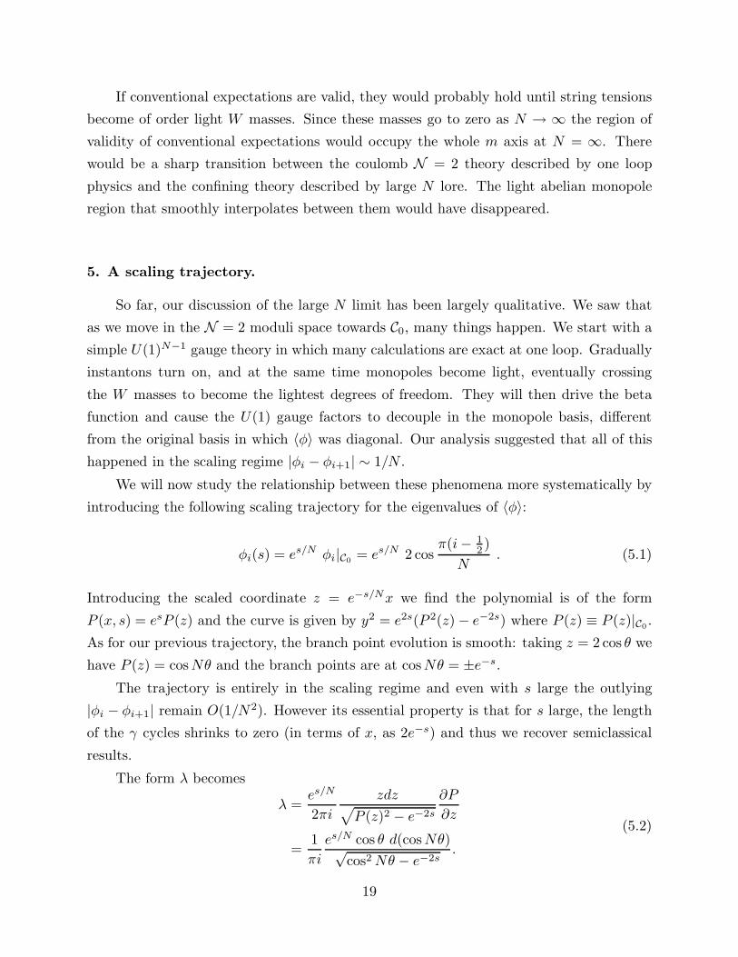
5. A scaling trajectory.

So far, our discussion of the large N limit has been largely qualitative. We saw that

as we move in the N = 2 moduli space towards C0, many things happen. We start with a

simple U(1)N−1 gauge theory in which many calculations are exact at one loop. Gradually

instantons turn on, and at the same time monopoles become light, eventually crossing

the W masses to become the lightest degrees of freedom. They will then drive the beta

function and cause the U(1) gauge factors to decouple in the monopole basis, different

from the original basis in which 〈φ〉 was diagonal. Our analysis suggested that all of this

happened in the scaling regime |φi − φi+1| ∼ 1/N .

We will now study the relationship between these phenomena more systematically by

introducing the following scaling trajectory for the eigenvalues of 〈φ〉:

φi(s) = es/N φi|C0= es/N 2 cos

π(i − 12)

N. (5.1)

Introducing the scaled coordinate z = e−s/Nx we find the polynomial is of the form

P (x, s) = esP (z) and the curve is given by y2 = e2s(P 2(z) − e−2s) where P (z) ≡ P (z)|C0.

As for our previous trajectory, the branch point evolution is smooth: taking z = 2 cos θ we

have P (z) = cos Nθ and the branch points are at cosNθ = ±e−s.

The trajectory is entirely in the scaling regime and even with s large the outlying

|φi − φi+1| remain O(1/N2). However its essential property is that for s large, the length

of the γ cycles shrinks to zero (in terms of x, as 2e−s) and thus we recover semiclassical

results.

The form λ becomes

λ =es/N

2πi

zdz√

P (z)2 − e−2s

∂P

∂z

=1

πi

es/N cos θ d(cos Nθ)√cos2 Nθ − e−2s

.

(5.2)

19

cosN� �e�s�e�s � �2�1The large N simplification occurs because the integrals over the α and γ cycles only cover a

range of θ ∼ 1/N . Thus we can expand the cos θ factor to isolate the leading N dependence.

For ai and aDm we obtain* (using u = cos Nθ)

ai =es/N 2 cos θi

π

∫ e−s

−e−s

du√e−2s − u2

+ O(1

N2) .

= es/N 2 cos θi

(5.3)

and

aDm =4i sin θm

πes/N (

1

NI1(s) + O(

1

N3))

=4ises/N

Nsin θm .

I1(s) =

∫ u=1

u=e−s

du arccos u√u2 − e−2s

= s .

(5.4)

We see that we can make monopoles much heavier than W ’s along this trajectory.

Monopole masses are comparable to the lightest W they couple to for s ∼ 1. One loop

contributions going like log(a/Λ) will show s dependence ∼ s/N , and we see from (5.4)

that at leading order in N the monopole and W masses are given exactly by the one loop

result, all the way to the massless monopole point! (We will see below that this is a special

property of this trajectory and more generally trajectories δφi ∼ cos πk(i − 12 )/N with

k ∼ O(N0).)

* The integral I1(s) is most easily evaluated by using partial integration to establish I1(s) =

−I1(−s). The only solution to this compatible with the analytic properties of I1 is I1 = s. We

are grateful to Alyosha and Sasha Zamolodchikov for providing this argument.

20

To compute τ , we might use

∂λ

∂φi=

es/N

2π

sin θ

cos θ − cos θi

cos Nθ√cos2 Nθ − e−2s

dθ. (5.5)

There is a subtlety in the large N expansion of this form, due to the pole in the prefactor

at θ = θi. Although the pole itself is cancelled by a zero of cosNθ, it is not justified to

treat the prefactor as slowly varying.

We will deal with this by using the basis of variations

∂λ

∂tk≡

N∑

i=1

∂λ

∂φicos

πk(i − 12)

N, (5.6)

We will find that using this basis for ‘electric’ quantities and the basis sin kθm for ‘magnetic’

quantities, the period matrices become simple and the kinetic term diagonal, for all s and

at finite N .

Before doing this in detail, let us suggest why this gives simple results. From (A.1)

and related formulas, it is clearly an appropriate basis for the massless monopole point

s = 0. On the other hand, the large s limit is expected to reproduce the semiclassical

results ∂ai/∂φj = δij and ∂aDi/∂φj = ∂2F/∂ai∂aj. From (2.3) and (5.3) this is

∂aDi

∂φj

∣

∣

∣

∣

one loop

= τ(1)ij =

i

2π

δij

∑

k 6=i

tik − (1 − δij)tij

tij =2s

N+ log(2 cos θi − 2 cos θj)

2.

(5.7)

The point is that the one-loop kinetic term is also diagonal in the cosine basis, by results

similar to those in the appendix, making it possible for τ along the entire trajectory to be

diagonal. Let us estimate its eigenvalues in the large N limit: the difference ti+1,j − ti,j ∼Bm=i,j +O(1/N) and so (A.1) implies that tij will have eigenvalues tκ ∼ 1

2 sin πk/N . (There

are corrections to this estimate, of O(k/N)).

We proceed to compute the periods of

∂λ

∂tk≡

N∑

i=1

∂λ

∂φicos

πk(i − 12 )

N

=1

2π

N sin(N − k)θ√cos2 Nθ − e−2s

dθ.

(5.8)

21

We have (a = arccos e−s, b = arcsin e−s, κ = k/N)

Ajk(s) =∂aj

∂tk=

(−1)j−1

π

∫ b

−b

dθsin((N − k)(θj + θ/N))

√

e−2s − sin2 θ

=1

π

∫ b

−b

dθcos kθj cos(1 − κ)θ + sin kθj sin(1 − κ)θ

√

e−2s − sin2 θ

= F (κ, s) cos kθj

F (κ, s) =1

π

∫ b

−b

dθcos(1 − κ)θ

√

e−2s − sin2 θ

→ 1

πsin

πκ

2(− log s) + 1 − O(κ) s → 0

→ 1 +κ(2 − κ)

4e−2s + . . . s → ∞

(5.9)

and similarly

Bmk(s) =∂aDm

∂tk= G(κ, s) sin kθm

G(κ, s) =1

π

∫ a

−a

dθ′cos(1 − κ)θ′√cos2 θ′ − e−2s

→ 1 +κ(2 − κ)

2s + . . . s → 0

→ 2s sinπκ

2+ 1 − O(κ) + . . . s → ∞.

(5.10)

We can now compute τDmn(s). Using (A.5) we see that τDmn(s) is diagonal in the

sin kθm basis:

τDmn(s) =∑

k

AmkB−1kn =

∑

i,k

q−1miAikB−1

kn ,

∑

n

τDmn(s) sin kθn = τDκ(s) sin kθm

(5.11)

with eigenvalues

τDκ(s) =1

2 sin πκ2

F (κ, s)

G(κ, s). (5.12)

We verify that τDκ(s) → − 12π log s, independent of κ, as s → 0. Similarly

τij(s) =∑

m,k

h−1imBmkA−1

kj

∑

j

τij(s) cos kθj = τκ(s) cos kθi

τκ(s) =1

2 sin πκ2

G(κ, s)

F (κ, s).

(5.13)

22

These formulae give an exact description of the physics along the scaling trajectory from

the semiclassical domain all the way to C0, even at finite N .

Note the crucial fact that the eigenvalues τκ(s) are not simply the inverses of the

eigenvalues τDκ(s)! The change of basis from electric (ij) to magnetic (mn) couplings

introduces an extra 14 sin2 πκ

2

. This will have important consequences and seems quite

mysterious; it may be relevant that (for example) in the magnetic basis, the W bosons

responsible for the one loop contribution to τ have charges with alternating signs (such as

(1 − 1 − 1 1) ), and in summing their loop effects there will be large cancellations.

Let us consider the leading correction to the logarithm from the monopole beta func-

tion at small s, which come from the constant terms in F and G:

τDκ(s) = − 1

2πlog s +

1

2 sin πκ2

+ O(1) + . . . . (5.14)

For k ∼ O(N0) (κ ∼ 1/N) and s ∼ O(N0), this is a large correction, of O(N). It

is a threshold effect and eventually the monopole-induced running of the coupling will

overwhelm it, but we need to go to scales s ∼ e−N for this to happen. Thus these effects

are quite important at large N .

The same constants are responsible for the s-independent term at large s in

τκ(s) = 2s +1

2 sin πκ2

+ O(1) + . . . . (5.15)

We see by comparison with (5.7) that this is just τone loop. Rather magically, the low k

‘modes’ manage to be simultaneously weak in electric and magnetic variables.

Since the constant term in τDκ has the same form, the form of τD in the monopole

basis can be inferred by analogy to τ :

τDmn ∼ − i

2πδmn log s +

i

2πlog(2 sin θm − 2 sin θn)2 + O(1) + . . . . (5.16)

This matrix is not diagonal and so a ‘magnetic observer’ would see peculiar transitions

between the m quanta. This observer might posit the existence of light solitons carrying

dual charge in four m factors (as mentioned above) that would mediate these transitions.

The similarity of (5.16) to the one-loop electric τ is very intriguing and leads us to

wonder if there is any sense in which it is a one-loop effect. The theory is certainly much

more ‘self-dual’ than one would have guessed.

We now plot the scaling functions to illustrate their structure. Note that the − 12π log s

behavior characteristic of the monopole one loop beta function sets in around s = 1

uniformly in κ. This is just at the energy scale set by the inverse ‘size’ of the monopole, as

23

-7.5 -5 -2.5 2.5 5 7.5

1

2

3

4

5

6

7

τ D κ

κ = e −3

κ = e −

κ = e −

2

1

− log s

discussed earlier. The large residual s independent term in (5.14) is responsible for the κ

dependent offsets of the curves. It is clear from the graph that one must go to s ∼ e−1/κ

before this offset is negligible.

The off diagonal terms in (5.16) influence the energies of states in the confining phase

obtained by adding the N = 2 breaking perturbation NmTrA2. The basic structure

of the flux tubes is determined by the monopole condensate which is determined from

the superpotential alone and hence does not depend on τDmn. It is still given by (2.19).

The string tensions do depend on τDmn and will be affected by the mixings described by

(5.16). We have not yet studied this problem, but we have examined the closely related

problem of the dual photon masses, by numerically diagonalizing the mass matrix. We

found that the quantitative relation (2.20) is altered but that the scales of the masses

remain unchanged. We expect the same for the string tensions. Note that these changes

are significant for m ∼ e−N , far below the energies where string breaking due to light W

pairs occur (m ∼ 1/N4).

We remind the reader that some quantities (ai and aDm) were exact at one loop along

the scaling trajectory. This occurred because the corrections to the one-loop results for

their derivatives, from (5.9)-(5.10), were suppressed by powers of κ, so would happen for

24

any trajectory with κ ∼ 1/N . If the same thing happened in other large N (supersym-

metric) theories, for even a single trajectory into the true ground state (here the massless

monopole point), it would have the important consequence that the ground state could be

found just knowing the one-loop effective action.

6. Conclusions

Using the solution of N = 2 supersymmetric SU(N) gauge theory of [2,3,4], we have

given an overview of some of the physics visible in the low energy effective Lagrangian. In

particular we studied the N = 1 theory obtained by giving a mass to the chiral superfield,

and extended Seiberg and Witten’s explicit derivation of a monopole condensation model

of confinement for SU(2) to SU(N).

The Lagrangian relevant for this confining theory is a weakly coupled U(1)N−1 gauge

theory with one light monopole hypermultiplet in each factor. The SN discrete gauge sym-

metry that permutes the U(1) factors is spontaneously broken. This phenomenon pervades

the physics of this system. In particular, there is a spectrum of different string tensions in

the different factors, κn ∼ mΛN sin πnN

and a spectrum of different light W boson masses

∼ ΛN sin πn

N that connect the factors. This differs in many ways from our expectations

about the pure N = 1 theory. It is possible for a dramatic but smooth rearrangement to

take place for m ∼ Λ that will connect these two descriptions. Perhaps this rearrangement

can be understood as a smooth crossover from a regime of spontaneously broken SN gauge

symmetry to one where the SN gauge symmetry is ‘confined.’

We studied the large N limit in detail. The hierarchy of scales present for finite N

becomes very large, as the lightest W mass ∼ Λ/N2. We found one signature of these very

light particles in the monopole ‘size’ which controls the energy scale of onset of pertur-

bative monopole coupling constant renormalization. Another very surprising signature is

the off-diagonal terms in (5.16) which cause a coupling of the different magnetic factors.

Understanding this phenomenon from the magnetic point of view, presumably as the result

of light electric solitons in a weakly coupled magnetic theory, would be very interesting.

At large N the one loop result becomes exact almost everywhere on the N = 2 moduli

space. We identified a scaling regime very close (∼ 1/N) to the massless monopole point

C0 where instanton and monopole effects survive the large N limit and were able to give

simple exact formulas for monopole and W masses and coupling constants along a scaling

trajectory through this regime.

The coupling almost everywhere on the N = 2 moduli space is 1/N , as expected, but

near C0 becomes large, contradicting standard large N lore. The infrared divergence of the

25

effective U(1) couplings, which does not commute with the large N limit, is the source of

this. Such a phenomenon would seem to apply to any continuous monopole condensation

picture of confinement, supersymmetric or otherwise. The region of this violation goes to

zero as N → ∞.

In the confining ‘almost N = 2’ theory, the abelian flux tube picture breaks down

because of W pair creation when confining scales become comparable to W scales. This

occurs for m ∼ Λ/N4, i.e., a vanishingly small region of the m axis. Conventional large N

lore could be recovered in a smooth, complicated crossover we cannot control. As N → ∞the region described by nontrivial light monopole physics shrinks to zero, possibly leaving

an abrupt transition between one loop physics and large N pure N = 1 SYM behavior.

Some features of this model are reminiscent of standard hadronic phenomenology

while others look very different (such as the weakly coupled glueballs), but overall we find

the results encouraging for the idea of using supersymmetric gauge theory as a solvable

starting point for attempts to model QCD dynamics. Surely interesting supersymmetric

analogs of many other problems of strongly coupled gauge theory and QCD physics can

be found, and we believe it will be very fruitful to study them using these techniques.

It is a pleasure to thank Philip Argyres, Tom Banks, Dan Friedan, Ken Intriliga-

tor, Wolfgang Lerche, John Preskill, Lisa Randall, Nati Seiberg and Alyosha and Sasha

Zamolodchikov for valuable conversations.

We are informed by Greg Moore that he and Mans Henningson have independently

obtained some of these results.

This research was supported in part by DOE grant DE-FG05-90ER40559, NSF PHY-

9157016 and the A. P. Sloan Foundation.

Appendix A. Trigonometric identities.

In section 2 we use

N−1∑

m=1

Bmi sinπkm

N= cos

πk(i− 12)

N(A.1)

which can be checked by writing (zm = eiθm , wi = eiθi)

Bmi =1

iN

(

1

1 − wizm− 1

1 − wiz−1m

)

. (A.2)

26

We convert the sum to run from 0 to 2N − 1, for which∑

m eπikm/N = 2Nδk,0(mod2N), by

taking a sum∑N−1

m=1 involving the second term in (A.2) and taking m → 2N − m. Then

N−1∑

m=1

Bmi sinπkm

N=

1

2N

2N−1∑

m=1

w−1i

w−1i − zm

(

e−iπkm/N − eiπkm/N)

=wk

i

1 − w2Ni

− w2N−ki

1 − w2Ni

=wk

i + w−ki

2.

(A.3)

Using (A.1), the orthogonality of the basis sinπkm/N under∑N−1

m=1, and the orthog-

onality of the basis cos πk(i− 12)/N under

∑Ni=1, we also have

N∑

i=1

Bmi cos kθi = sin kθm. (A.4)

In section 5 we use the change of basis

∑

m

qmi sin kθm = sin kθm=i − sin kθm=i−1 = 2 sin

kπ

2Ncos kθi (A.5)

We next evaluate the sum

fk(θ) =1

N

N∑

j=1

sin θ

cos θj − cos θcos kθj =

sin(N − k)θ

cos Nθ. (A.6)

First, for k = 0, the sum is

1

N

∂

∂θlog

∏

j

(cos θj − cos θ) =1

N

∂

∂θlog P (x) = tanNθ. (A.7)

For k integer, the sum is a periodic function of θ with residues cos kθ at the points θ = θj,

so it must take the form

fk(θ) = tanNθ cos kθ + finite. (A.8)

From the above, the finite part is known at the points θ = θm to be − sin kθ. This is true

of the function

fk(θ) = tanNθ cos kθ − sin kθ (A.9)

(equal to (A.6)) plus any periodic function vanishing at all of the θm, such as sin 2Nlθ.

Such terms can be excluded by considering the derivative d/dθ at θ = 0.

27

References

[1] N. Seiberg, Nucl. Phys. B435 (1995)129, hep-th/9411149 and references therein. For

a brief review, see “The Power of Holomorphy,” N. Seiberg, hep-th/9408013.

[2] N. Seiberg and E. Witten, Nucl.Phys. B426 (1994) 19. The generalization to theories

with matter hypermultiplets is discussed in N. Seiberg and E. Witten, hep-th/9408099.

[3] P. C. Argyres and A. E. Faraggi, hep-th/9411057.

[4] A. Klemm, W. Lerche, S. Yankielowicz and S. Theisen, hep-th/9411048 and hep-

th/9412158.

[5] N. Seiberg, Phys. Lett. 206B (1988) 75.

[6] G. ’t Hooft, Nucl. Phys. B190 [FS3] (1981) 455.

[7] S. Cecotti, P. Fendley, K. Intriligator, and C. Vafa, Nucl. Phys. B386 (1992) 405; S.

Cecotti and C. Vafa, Comm. Math. Phys. 158 (1993) 569.

28