Semiclassical analysis of the phases of 4d SU(2) Higgs

gauge systems with cutoff at the Gribov horizon

M. A. L. Capria∗, D. Dudalb†, A. J. Gomeza‡, M. S. Guimaraesa§, I. F. Justo a¶,S. P. Sorellaa‖, D. Vercauterena∗∗††

a Departamento de Fısica Teorica, Instituto de Fısica, UERJ - Universidade do Estado do Rio de Janeiro,

Rua Sao Francisco Xavier 524, 20550-013 Maracana, Rio de Janeiro, Brasilb Ghent University, Department of Physics and Astronomy, Krijgslaan 281-S9, 9000 Gent, Belgium

Abstract

We present an analytical study of continuum 4d SU(2) gauge Higgs models with a single Higgsfield with fixed length in either the fundamental or adjoint representation. We aim at analyticallyprobing the renowned predictions of Fradkin & Shenker on the phase diagram in terms of confinementversus Higgs behaviour, obtained for the lattice version of the model. We work in the Landau versionof the ’t Hooft Rξ gauges in which case we can access potential nonperturbative physics related tothe existence of the Gribov copies. In the fundamental case, we clearly show that in the perturbativeregime of small gauge coupling constant g and large Higgs vacuum expectation value ν, there is a Higgsphase with Yukawa gauge boson propagators without Gribov effects. For a small value of the Higgsvev ν and/or large g, we enter a region with Gribov type propagators that have no physical particleinterpretation: the gauge bosons are as such confined. The transition between both behaviours isfound to be continuous. In the adjoint case, we find evidence of a more drastic transition between thedifferent behaviours for the propagator of the off-diagonal gauge bosons, whereas the “photon”, i.e. thediagonal component of the gauge field, displays a propagator of the Gribov type. In the limit of infiniteHiggs condensate, we show that a massless photon is recovered. We compare our findings with those ofFradkin & Shenker as well as with more recent numerical lattice simulations of the fundamental Higgsmodel. We also carefully discuss in which region of the parameter space (ν, g) our approximations aretrustworthy.

1 Introduction

The understanding of the transition between the confinement and the Higgs phase of asymptoticallyfree nonabelian gauge theories in presence of Higgs fields is a relevant and yet not fully unraveled topic.Needless to say, such theories are the building blocks of the Standard Model.

∗caprimarcio@gmail.com†david.dudal@ugent.be‡ajgomez@uerj.br§msguimaraes@uerj.br¶igorfjusto@gmail.com‖sorella@uerj.br∗∗vercauteren.uerj@gmail.com††Work supported by FAPERJ, Fundacao de Amparo a Pesquisa do Estado do Rio de Janeiro, under the program Cientista

do Nosso Estado, E-26/101.578/2010.

1

arX

iv:1

212.

1003

v2 [

hep-

th]

2 A

pr 2

013

Numerical studies of the lattice version of these models [1, 2, 3, 4, 5, 6, 7, 8, 9] have already revealeda rich structure of the corresponding phase diagram, as well as mean-field approaches to the underlyinglattice models as in [10, 11, 12]. What emerges from the lattice works is that the transition between theconfinement and the Higgs phase strongly depends on the representation of the Higgs field.

In the case of the fundamental representation, it turns out that these two phases can be continuouslyconnected, i.e. they are not completely separated by a transition line. For the benefit of the reader, it isworth spending a few words on this statement. We follow here the seminal work by [1], where the latticeversion of the model has been considered for a Higgs field with fixed length, i.e. by freezing its radial part.This amounts to keep the Higgs quartic self-coupling very large, not to say infinite, so that the Higgs fieldis frozen to its vev. The resulting theory has two basic parameters, the gauge coupling g and the vev ν ofthe Higgs field. In the plane (ν, g), the Higgs phase corresponds to the region of weak coupling, i.e. smallg and sufficiently large ν. In this region, the Wilson loop exhibits a perimeter law and the force betweentwo static sources is short ranged. Instead, the confining phase corresponds to the strong coupling regionin the (ν, g) plane, characterized by large values of g and sufficiently small ν. Here, the Wilson loop givesrise to a linear potential over some finite distance region, followed by string breaking via scalar particleproduction. It turns out that these two regions are smoothly connected. More precisely, from e.g. Fig.1of [6], one learns that the confining and Higgs phases are separated by a first order line transition which,however, does not extend to the whole phase diagram. Instead, it displays an endpoint. This impliesthat the Higgs phase can be connected to the confining phase in a continuous way, i.e. without crossingthe transition line. Even more striking, one observes a region in the (ν, g) plane, called analyticity region[1, 5, 6], in which the Higgs and confining phases are connected by paths along which the expectationvalue of any local correlation function varies analytically, implying the absence of any discontinuity inthe thermodynamical quantities. According to [1], the spectrum of the theory evolves continuously fromone regime to the other. Said otherwise, the physical states in both regimes are generated by suitablegauge invariant operators which, in the Higgs phase, give rise to massive bosons while, in the confiningphase, to a meson like state, i.e. to a bound state of confined excitations. We shall stick to the use ofthe word “phase” here, although it is clear there cannot exist a local order parameter1 discriminatingbetween the Higgs or confinement behaviour.

In the adjoint Higgs case, the breaking or not of center symmetry and associated Polyakov loopexpectation value can in principle be used to discriminate between phases, leading to (an) expectedphase transition(s) between confining and Higgs behaviour, as already put forward in [1] and tested ine.g. [2]. Moreover, as speculated in [1], the appearance of an in some cases expected Coulomb phase withlong-range correlations was not reported. Over the years, most attention has however been paid to thefundamental Higgs, due to its more direct physical relevance for the electroweak physics.

The attentive reader will have noticed that most of the cited works either concern lattice simulationsof the gauge Higgs systems, or analytical semiclassical mean-field analysis of the lattice model. There isa good reason for this as the probed physics is usually of a nonperturbative nature. Some preliminaryfunctional Dyson-Schwinger approaches to gauge field theories supplemented with scalar fields have ap-peared nonetheless [13, 14], however these do not really touch upon the supposed phase diagram andthe analyticity results of Fradkin & Shenker. Direct computation of phase diagram related quantities asPolyakov loops or even the vacuum (free) energy are noteworthy hard to access at the functional level.Let us by the way notice here that the proof of the Fradkin-Shenker analyticity result, inspired by [15],heavily relies on the lattice formulation of the problem. We are unaware of a strict continuum versionof the theorem, although one might expect it to hold as well. It is in any case a strong property of thetheory if it would be analytical in a certain region of the phase diagram. In some cases, the Fradkin

1Nor can the Polyakov loop P serve as an order parameter since the presence of a fundamental Higgs field breaks thecenter symmetry in a hard way, giving anyhow a nontrivial expectation value to P.

2

& Shenker result has been related to the Lee-Yang theorem that also handles analyticity properties ofstatistical systems [16, 17]. One can imagine a lot of subtleties making any concrete analytical studyof the Higgs phase diagram troublesome. To name only one, renormalization will require to considerthe gauge coupling constant at a particular renormalization scale and the issue of strong versus weakcoupling is directly set by the size of this scale. We will come back to this issue later.

The aim of this work is that of investigating the transition between the Higgs and the confinementphase within a continuum quantum field theory. The set up which we shall follow is that of takinginto account the nonperturbative effect of the existence of the Gribov copies [18] which are unavoidablypresent in the gauge fixing quantization procedure2. In particular, as already shown in the case of three-dimensional gauge theories [21], this framework enables us to encode nonperturbative information aboutthe phases of the theory in the two-point correlation function of the gauge field in momentum space. Thetransition between one phase to another is detected by the corresponding change in the pole structure ofthe gluon propagator. More precisely, a gluon propagateor of the Gribov type, i.e. displaying complexconjugate poles, has no particle interpretation, being well suited to describe the confining phase. On theother hand, a propagator of the Yukawa type, i.e. displaying a real pole in momentum space, means thatthe theory is located in the Higgs phase.

By quantizing the theory in the Landau gauge and by performing the restriction to the so calledGribov region Ω [18, 19, 20] in order to take into account the effect of the Gribov copies, we shall beable to discuss the changes in the gluon propagator when the parameters (ν, g) are varied from the Higgsweak coupling region to the confining strong coupling region. As we shall see in details, in the case ofthe fundamental representation we shall be able to detect a region in the (ν, g) plane, characterized bythe line3 a = 1

2 , with

a =g2ν2

4µ2e

(1− 32π2

3g2

) . (1)

The Higgs region will correspond to values of (ν, g) for which a > 12 , while the confining phase will be

located in the region a < 12 . Moreover, the gluon propagator evolves in a smooth continuous way from the

confining to the Higgs region, namely we observe a continuous evolution of the poles of the propagatorfrom a Gribov type to the Yukawa behavior. In addition, we shall be able to evaluate the vacuum energyin Gribov’s semiclassical approximation and check explicitly that it is a continuous function, togetherwith its first and second derivative, of the parameter a across the transition line a = 1

2 . The thirdderivative of the vacuum energy displays a discontinuity across a = 1

2 . However, we shall be able tocheck that the line a = 1

2 is not located in the Fradkin-Shenker analyticity region, something which wecannot access within the present approximation as a = 1

2 corresponds to a region wherein we cannotreally trust the made approximations. Though, we are able to confirm within a continuum field theorythat the transition between the Higgs and the confining phase occurs in a smooth way, something whichis far from being trivial. Another relevant result of our analysis is that, in the Higgs phase, there is noneed to implement the restriction to the Gribov region Ω. Said otherwise, in the Higgs phase, the valuesof the parameters (ν, g) are such that the theory automatically lies within the Gribov region Ω, so thatthe Gribov horizon is never crossed. This is a quite relevant observation which has an important physicalconsequence. It ensures that, in the weak coupling region, the standard Higgs mechanism takes placewithout being affected by the restriction to the Gribov region. We have thus a truly nonconfining theorywhose asymptotic states are the massive gauge bosons.

When the Higgs field is in the adjoint representation, our results indicate that things change drasti-cally, as also expected from lattice investigations. Here, the phase structure looks much more intricate as

2See [19, 20] for a pedagogical introduction to the Gribov problem.3The quantity µ stands for the energy scale which shows up in the renormalization of ultraviolet divergent quantities. In

the present case, dimensional regularization in the MS scheme is employed.

3

well as the evolution of the two-point correlation function of the gauge field. In addition of the confiningphase, in which the gluon propagator is of the Gribov type, we shall find what can be called a U(1)confining phase, in which the third component A3

µ of the gauge field displays a Gribov type correlationfunction, while the remaining off-diagonal components, Aαµ, α = 1, 2, are of the Yukawa type. It is worthnoticing here that this phase has been reported in lattice investigations of the Georgi-Glashow model[22, 23], i.e. of three dimensional gauge theories with a Higgs field in the adjoint. Unfortunately, tillnow, we are unaware of lattice studies of the gluon propagator in four dimensions with Higgs field inthe adjoint4. So far, only the case of the fundamental representation has been addressed [7, 8]. Fromthat point of view, we hope that our results will stimulate further studies of the gluon propagator on thelattice in order to confirm the existence of the U(1) confining phase in four dimensions, to the extent thatthe diagonal gauge boson propagator is not of the massless type for finite value of the Higgs condensate.A lattice study of the adjoint Higgs phase diagram was presented in [24], giving evidence of a masslessCoulomb phase in the limit of infinite Higgs condensate ν. More precisely, the theory was shown toreduce to a compact U(1) model with its confinement-deconfinement transition. We do however notexpect such a transition in the continuum version of QED. We shall see that in the limit ν →∞ we canhowever recover also a massless photon. This is not as trivial a result as it might appear since it involvesa delicate cancelation between diverging Higgs condensate and vanishing Gribov parameter.

The paper is organized as follows. In Sect. 2 we discuss the restriction to the Gribov region in thecase of the fundamental representation. The behavior of the gluon propagator and of the vacuum energyare discussed within Gribov’s approximation. In Sect. 3 we address the more intricate case of the Higgsfield in the adjoint representation. Sect. 4 collects our conclusion.

2 Restriction to the Gribov region Ω with a fundamental Higgs field

Let us consider first the case of SU(2) Yang-Mills theories interacting with Higgs fields in the fundamentalrepresentation. This will be the most interesting case for future reference as well, when the physical caseof SU(2)× U(1) will be analyzed, i.e. the electroweak theory.

Working in Euclidean space and adopting the Landau gauge, ∂µAaµ = 0, the action of the current

model is specified by the following expression

S =

∫d4x

(1

4F aµνF

aµν + (Dij

µ Φj)†(Dikµ Φk) +

λ

2

(Φ†Φ− ν2

)2+ ba∂µA

aµ + ca∂µD

abµ c

b

), (2)

where the covariant derivative is defined by

Dijµ Φj = ∂µΦi − ig (τa)ij

2AaµΦj . (3)

The field ba stands for the Lagrange multiplier implementing the Landau gauge, ∂µAaµ = 0, while (ca, ca)

are the Faddeev-Popov ghosts. The indices i, j = 1, 2 refer to the fundamental representation, andτa, a = 1, 2, 3, are the Pauli matrices. The vacuum configuration which minimizes the energy is achievedby a constant scalar field parameterized as

〈Φ〉 =

(0ν

), (4)

It will be understood that we work in the limit λ→∞ for simplicity, i.e. we have a Higgs field frozen atits vacuum expectation value, as in [1].

4Adjoint lattice gauge-Higgs systems have been studied in e.g. [2, 25] but not directly from the propagator viewpoint.

4

All components of the gauge field acquire the same mass m2 = g2ν2

2 . In fact, for the quadratic partof the action we have now

Squad =

∫d4x

(1

4

(∂µA

aν − ∂νAaµ

)2+ ba∂µA

aµ +

g2ν2

4AaµA

aµ

). (5)

As already mentioned in the Introduction, the aim of the present work is that of analyzing the possiblenonperturbative dynamics of the model by taking into account the Gribov copies. In the Landau gauge5,this issue can be faced by restricting the domain of integration in the path integral to the so called Gribovregion Ω [18, 19, 20], defined as the set of all transverse gauge configurations for which the Faddeev-Popovoperator is strictly positive, namely

Ω = Aaµ , ∂µAaµ = 0 , −∂µDabµ > 0 . (6)

The region Ω is known to be convex and bounded in all directions in field space. The boundary of Ω,where the first vanishing eigenvalue of the Faddeev-Popov operator appears, is called the first Gribovhorizon. A way to implement the restriction to the region Ω has been worked out by Gribov in hisoriginal work. It amounts to impose the no-pole condition [18, 19, 20] for the connected two-point

ghost function Gab(k;A) = 〈k|(−∂Dab(A)

)−1 |k〉, which is nothing but the inverse of the Faddeev-Popovoperator −∂Dab(A). One requires that Gab(k;A) has no poles at finite nonvanishing values of k2, so thatit stays always positive. In that way one ensures that the Gribov horizon is not crossed, i.e. one remainsinside Ω. The only allowed pole is at k2 = 0, which has the meaning of approaching the boundary of theregion Ω.

Following Gribov’s procedure [18, 19, 20], for the connected two-point ghost function Gab(k;A) atfirst order in the gauge fields, one finds

Gab(k;A) =1

k2

(δab − g2kµkν

k2

∫d4q

(2π)4εamcεcnb

1

(k − q)2(Amµ (q)Anν (−q)

)), (7)

where use has been made of the transversality condition qµAµ(q) = 0. Taking into account that all massesof the gauge field are degenerate in color space, eq.(5), we introduce the ghost form factor σ(k;A) as

G(k;A) =δabGab

3=

1

k2

(1 +

kµkνk2

2g2

3

∫d4q

(2π)4Aaµ(q)Aaν(−q)

(q − k)2

)≡ 1

k2(1 + σ(k;A)) ≈ 1

k2

(1

1− σ(k;A)

). (8)

The quantity σ(k;A) turns out to be a decreasing function of the momentum k [18, 19, 20]. Thus, theno-pole condition for the ghost function G(k,A) is implemented by imposing that [18, 19, 20]

σ(0;A) ≤ 1 , (9)

where σ(0;A) is given by

σ(0;A) =g2

6

∫d4q

(2π)4Aaµ(q)Aaµ(−q)

q2. (10)

5 It is perhaps worthwhile pointing out here that the Landau gauge is also a special case of the ’t Hooft Rξ gauges,which have proven their usefulness as being renormalizable and offering a way to get rid of the unwanted propagator mixingbetween (massive) gauge bosons and associated Goldstone modes, ∼ Aµ∂µφ. The latter terms indeed vanish upon using thegauge field transversality. The upshot of specifically using the Landau gauge is that it allows to take into account potentialnonperturbative effects related to the gauge copy ambiguity.

5

This expression is obtained by taking the limit k → 0 of eq.(8), and by making use of the property

Aaµ(q)Aaν(−q) =

(δµν −

qµqνq2

)ω(A)(q)

⇒ ω(A)(q) =1

3Aaλ(q)Aaλ(−q) (11)

which follows from the transversality of the gauge field, qµAaµ(q) = 0. Also, it is useful to remind that,

for an arbitrary function F(p2), we have∫d4p

(2π)4

(δµν −

pµpνp2

)F(p2) = A δµν (12)

where, upon contracting both sides of eq.(12) with δµν ,

A =3

4

∫d4p

(2π)4F(p2). (13)

2.1 Gribov’s gap equations

In order to ensure the restriction to the Gribov region Ω in the functional integral, we encode theinformation of the no-pole conditions into a step function [18, 19, 20]:

Z =

∫[dA]δ(∂A) det(−∂Dab) θ(1− σ(0;A)) e−SYM . (14)

Though, as our interest for now lies only in the study of the gauge boson propagators, we shall considerhere the quadratic approximation for the partition function, namely

Zquad =

∫dϑ

2πiϑ[dA] eϑ(1−σ(0,A)) e

− 14

∫d4x(∂µAaν−∂νAaµ)2− 1

2ξ

∫d4x(∂µAaµ)

2− g2ν2

4

∫d4xAaµA

aµ , (15)

where use has been made of the integral representation

θ(x) =

∫ i∞+ε

−i∞+ε

dϑ

2πiϑeϑx . (16)

The extension of this work beyond the semiclassical approximation can be worked out using the toolsof [20]. We shall also not dwell upon renormalization details here, we expect that the proof of the puregauge case as in [20, 26] can be suitably adapted.

After simple algebraic manipulations, one gets for (15)

Zquad =

∫dϑeϑ

2πiϑ[dA] e

− 12

∫ d4q

(2π)4Aaµ(q)PabµνAbν(−q), (17)

with

Pabµν = δab(δµν

(q2 +

ν2g2

2

)+

(1

ξ− 1

)qµqν +

ϑ

3

g2

q2δµν

). (18)

The parameter ξ is understood to be zero at the end in order to recover the Landau gauge. Evaluatingthe inverse of the expression above and taking the limit ξ → 0, for the gluon propagator one gets⟨

Aaµ(q)Abν(−q)⟩

= δabq2

q4 + g2ν2

2 q2 + g2

3 ϑ

(δµν −

qµqνq2

). (19)

6

It remains to find the gap equation for the Gribov parameter ϑ, enabling us to express it in terms of theparameters of the starting model, i.e. the gauge coupling constant g and the vev of the Higgs field ν.In order to accomplish this task we follow [18, 19, 20] and evaluate the partition function Zquad in thesemiclassical approximation. First, we integrate out the gauge fields, obtaining

Zquad =

∫dϑ

2πie(ϑ−lnϑ)

(detPabµν

)− 12. (20)

Making use of (detPabµν

)− 12

= e−12ln detPabµν = e−

12Tr lnPabµν , (21)

for the determinant in expression (20) we get(detPabµν

)− 12

= exp

[−9

2

∫d4q

(2π)4ln

(q2 +

g2ν2

2+g2ϑ

3

1

q2

)]. (22)

Therefore,

Zquad =

∫dϑ

2πief(ϑ) , (23)

where, in the thermodynamic limit6,

f(ϑ) = ϑ− 9

2

∫d4k

(2π)4ln

(k2 +

g2ν2

2+ϑ

3

g2

k2

). (24)

Expression (23) can be now evaluated in the saddle point approximation [18, 19, 20], i.e.

Zquad ≈ ef(ϑ∗) , (25)

where the parameter ϑ∗ is determined by the stationary condition

∂f

∂ϑ∗= 0 , (26)

which yields the following gap equation

3

2g2∫

d4q

(2π)41

q4 + g2ν2

2 q2 + g2

3 ϑ∗

= 1 . (27)

Notice also that the function f(ϑ∗) has the meaning of the vacuum energy Ev of the system. Moreprecisely

Ev = −f(ϑ∗) , (28)

as it is apparent from the expression of the partition function Zquad, eq.(25). To discuss the gap equation(27), we decompose the denominator according to

q4 +g2ν2

2q2 +

g2

3ϑ = (q2 +m2

+)(q2 +m2−) , (29)

with

m2+ =

1

2

(g2ν2

2+

√g4ν4

4− 4g2

3ϑ∗

), m2

− =1

2

(g2ν2

2−√g4ν4

4− 4g2

3ϑ∗

). (30)

6We remind here that the term lnϑ in expression (20) can be neglected in the derivation of the gap equation, eq.(27),when taking the thermodynamic limit, see [18, 19, 20] for details.

7

Making use of the MS renormalization scheme in d = 4− ε and of the standard integral∫ddp

(2π)d1

p2 + ρ2= − ρ2

16π22

ε+

ρ2

16π2

(lnρ2

µ2− 1

), (31)

for the gap equation (27) we consequently get(1 +

m2−

m2+ −m2

−ln

(m2−µ2

)−

m2+

m2+ −m2

−ln

(m2

+

µ2

))=

32π2

3g2. (32)

In order to analyze this equation we rewrite it in a more suitable way, i.e.

m2−

m2+ −m2

−ln

(m2−µ2

)−

m2+

m2+ −m2

−ln

(m2

+

µ2

)= −

m2+ −m2

−m2

+ −m2−

(1− 32π2

3g2

)=m2

+ −m2−

m2+ −m2

−ln

(e−(1− 32π2

3g2

)),

(33)so that

m2− ln

m2−

µ2e

(1− 32π2

3g2

) = m2

+ ln

m2+

µ2e

(1− 32π2

3g2

) , (34)

whose final form can be written as

2√

1− ζ ln(a) = −(

1 +√

1− ζ)

ln(

1 +√

1− ζ)

+(

1−√

1− ζ)

ln(

1−√

1− ζ), (35)

where we have introduced the dimensionless variables

a =g2ν2

4µ2e

(1− 32π2

3g2

) , ζ =16

3

ϑ∗

g2ν4≥ 0 , (36)

with 0 ≤ ζ < 1 in order to have two real, positive, distinct roots (m2+,m

2−), eq.(30). It is worth to

underline that the renormalization scale µ could be exchanged in favour of the invariant scale ΛMS,defined at one-loop as

Λ2MS

= µ2 e1β0

1g2(µ) , (37)

with β0 given by [27, 28]

β = −g3β0 +O(g5) , β0 =1

16π2

(11

3N − 1

6T

), (38)

where T is the Casimir of the representation of the Higgs field equaling T = 12 , resp. T = 2, for the

fundamental, resp. adjoint, representation of SU(2).

For ζ > 1, the roots (m2+,m

2−) become complex conjugate, and the gap equation takes the form

2√ζ − 1 ln(a) = −2 arctan

(√ζ − 1

)−√ζ − 1 ln ζ . (39)

Moreover, it is worth noticing that both expressions (35),(39) involve only one function, i.e. they can bewritten as

2 ln(a) = g(ζ) , (40)

where for g(ζ) we might take

g(ζ) =1√

1− ζ

(−(

1 +√

1− ζ)

ln(

1 +√

1− ζ)

+(

1−√

1− ζ)

ln(

1−√

1− ζ))

, (41)

which is a real function of the variable ζ ≥ 0. Expression (39) is easily obtained from (35) by rewritingit in the region ζ > 1. In particular, it turns out that the function g(ζ) ≤ −2 ln 2 for all ζ ≥ 0, andstrictly decreasing. As consequence, for each value of a < 1

2 , equation (40) has always a unique solutionwith ζ > 0. Moreover, it is easy to check that g(1) = −2. Therefore, we can distinguish ultimately threeregions, namely

8

(a) when a > 12 , eq.(40) has no solution for ζ. As the gap equation (27) has been obtained by acting

with ∂∂ϑ on the expression of the vacuum energy Ev = −f(ϑ), eq.(28), we are forced to set ϑ = 0.

This means that, when a > 12 , the dynamics of the system is such that the restriction to the Gribov

region cannot be consistently implemented. As a consequence, the standard Higgs mechanism takesplace, yielding three massive gauge fields, according to⟨

Aaµ(q)Abν(−q)⟩

= δab1

q2 + g2ν2

2

(δµν −

qµqνq2

). (42)

For sufficiently weak coupling g2, we underline that a will unavoidably be larger than 12 .

(b) when 1e < a < 1

2 , equation (40) has a solution for 0 ≤ ζ < 1. In this region, the roots (m2+,m

2−) are

real and the gluon propagator decomposes into the sum of two terms of the Yukawa type:⟨Aaµ(q)Abν(−q)

⟩= δαβ

(F+

q2 +m2+

− F−q2 +m2

−

)(δµν −

qµqνq2

), (43)

where

F+ =m2

+

m2+ −m2

−, F− =

m2−

m2+ −m2

−. (44)

Moreover, due to the relative minus sign in eq.(43) only the component F+ represents a physicalmode.

(c) for a < 1e , equation (40) has a solution for ζ > 1. This scenario will always be realized if g2

gets sufficiently large, i.e. at strong coupling. In this region the roots (m2+,m

2−) become complex

conjugate and the gauge boson propagator is of the Gribov type, displaying complex poles. Asusual, this can be interpreted as the confining region.

In summary, we clearly notice that at sufficiently weak coupling, the standard Higgs mechanism, eq.(42),will definitely take place, as a > 1

2 , whereas for sufficiently strong coupling, we always end up in aconfining phase because then a < 1

2 .

Having obtained these results, it is instructive to go back where we originally started. For a funda-mental Higgs, all gauge bosons acquire a mass that screens the propagator in the infrared. This effect,combined with a sufficiently small coupling constant, will lead to a severely suppressed ghost self energy,i.e. the average of (10) (to be understood after renormalization of course). If the latter quantity will apriori not exceed the value of 1 under certain conditions, the theory is already well inside the Gribovregion and there is no need to implement the restriction. Actually, the failure of the Gribov restrictionfor a > 1

2 is exactly because it is simply not possible to enforce that σ(0) = 1. Perturbation theory in theHiggs sector is in se already consistent with the restriction within the 1st Gribov horizon. Let us verifythis explicitly by taking the average of (10) with as tree level input propagator a transverse Yukawa one

with mass m2 = g2ν2

2 , cfr. eq. (5). Using that there are 3 transverse directions7 in 4d, we easily get

σ(0) =3g2

2

∫d4q

(2π)41

q2(q2 + g2ν2

2 )= − 3

ν2

∫d4q

(2π4)

1

q2 + g2ν2

2

= − 3g2

32π2

(lng2ν2

2µ2− 1

)(45)

7We have been a bit sloppy in this paper with the use of dimensional regularization. In principle, there are 3−ε transversepolarizations in d = 4 − ε dimensions. Positive powers in ε can (and will) combine with the divergences in ε−1 to changethe finite terms. However, as already pointed out before, a careful renormalization analysis of the Gribov restriction ispossible, see e.g. [26, 20] and this will also reveal that the “1” in the Gribov gap equation will receive finite renormalizations,compatible with the finite renormalization in e.g. σ(0), basically absorbable in the definition a. The main results of ourcurrent paper thus remain correct and we leave the full renormalization details for later.

9

Introducing a as in (36), we may reexpress the latter result as

σ(0) = 1− 3g2

32π2ln(2a) (46)

For a > 12 , the logarithm is positive and it is then evident that σ(0) will not cross 1, indicating that the

theory already is well within the first Gribov horizon.

Another interesting remark is at place concerning the transition in terms of a varying value of a. Ifa crosses 1

e , the imaginary part of the complex conjugate roots becomes smoothly zero, leaving us with2 coinciding real roots, which then split when a grows. At a = 1

2 , one of the roots and its accompanyingresidue vanishes, to leave us with a single massive gauge boson. We thus observe all these transitions arecontinuous, something which is in qualitative correspondence with the theoretical lattice predictions ofthe classic work [1] for a fundamental Higgs field that is “frozen” (λ → ∞). Concerning the somewhatstrange intermediate phase, i.e. the one with a Yukawa propagator with a negative residue, eq.(43), wecan investigate in future work in more detail the asymptotic spectrum based on the BRST tools developedin [29] when the local action formulation of the Gribov restriction is implemented.

2.2 The vacuum energy, phase transition and how trustworthy are the results?

Let us look at the vacuum energy Ev of the system, which can be easily read off from expression (23),namely

Ev = −ϑ∗ +9

2

∫d4k

(2π)4ln

(k2 +

g2ν2

2+ϑ∗

3

g2

k2

), (47)

where ϑ∗ is given by the gap equation (27). Making use of∫ddp

(2π)dln(p2 +m2) = − m4

32π2

(2

ε− ln

m2

µ2+

3

2

), (48)

it is very easy to write down the vacuum energy:

• for a < 12 , we have

8

9g4ν4Ev =

1

32π2

(1− 32π2

3g2

)− 1

2

ζ

32π2+

1

4

1

32π2

((4− 2ζ)

(ln(a)− 3

2

))(49)

+1

4

1

32π2

((1 +

√1− ζ

)2ln(

1 +√

1− ζ)

+(

1−√

1− ζ)2

ln(

1−√

1− ζ))

,

where ζ is obtained through eqs.(40),(41). Let us also give the expressions of the first two derivativesof Ev(a) with respect to a. From the gap equation (40), we easily get

∂ζ

∂a=

2

a

1

g′(ζ). (50)

Therefore

∂

∂a

[8

9g4ν4Ev]

=1

64π21

a(2− ζ) ,

∂2

∂a2

[8

9g4ν4Ev]

=1

64π21

a2

(ζ − 2− 2

g′(ζ)

). (51)

10

• for a > 12 ,

8

9g4ν4Ev =

1

32π2

(1− 32π2

3g2

)+

1

32π2

((ln(a)− 3

2

))+

1

32π2ln 2 . (52)

Owing to the fact that g′(0) = −∞, it turns out that vacuum energy Ev(a) is a continuous function of thevariable a, as well as its first and second derivative. The third derivative develops a jump at a = 1

2 . Wemight be tempted to interpret this is indicating a third order phase transition at a = 1

2 . The latter valueactually corresponds to a line in the (g2, ν) plane according to the functional relation (36). However, weshould be cautious to blindly interpret this value. It is important to take a closer look at the validity ofour results in the light of the made assumptions. More precisely, we implemented the restriction to thehorizon in a first order approximation, which can only be meaningful if the effective coupling constant issufficiently small, while simultaneously emerging logarithms should be controlled as well. In the absence

of propagating matter, the expansion parameter is provided by y ≡ g2N16π2 as in pure gauge theory. The

size of the logarithmic terms in the vacuum energy (that ultimately defines the gap equations) are set

by m2+ ln

m2+

µ2and m2

− lnm2−µ2

. A good choice for the renormalization scale would thus be µ2 ∼ |m2+|: for

(positive) real masses, a fortiori we have m2− < m2

+ and the second log will not get excessively largeeither because m2

− gets small and the prefactor is thus small, or m2− is of the order of m2

+ and the logitself small. For complex conjugate masses, the size of the log is set by the (equal) modulus of m2

± andthus both small by our choice of scale.

Let us now consider the trustworthiness, if any, of the a = 12 phase transition point. For a ∼ 1

2 , we

already know that ζ ∼ 0, so a perfect choice is µ2 ∼ m2+ ∼

g2ν2

2 . Doing so, the a-equation corresponds to

1

2∼ e−1+

43y (53)

so that y ∼ 4. Evidently, this number is thus far too big to associate any meaning to the “phase transition”at a = 1

2 . Notice that there is no problem for the a small and a large region. If ν2 is sufficiently large

and we set µ2 ∼ g2ν2

2 we have a small y, leading to a large a, i.e. the weak coupling limit without Gribovparameter and normal Higgs-like physics. The logs are also well-tempered. For a small ν2, the choiceµ2 ∼

√g2θ∗ will lead to

a ∼ (small number)e−1+ 4

3y (54)

so that a small a can now be compatible with a small y, leading to a Gribov parameter dominating the

Higgs induced mass, the “small number” corresponds to g2ν2√g2θ∗

. Due to the choice of µ2, the logs are

again under control in this case.

Within the current approximation, we are thus forced to conclude that only for sufficiently small orlarge values of the parameter a we can probe the theory in a controllable fashion. Nevertheless, this issufficient to ensure the existence of a Higgs-like phase at large Higgs condensate, and a confinement-likeregion for small Higgs condensate. The intermediate a-region is more difficult to interpret due to theoccurrence of large logs and/or effective coupling. Notice that this also might make the emergence of thisdouble Yukawa phase at a = 1

e ≈ 0.37 not well established at this point.

11

3 Restriction to the Gribov region Ω with an adjoint Higgs field

Let us face now the case in which the Higgs field Φa transforms according to the adjoint representationof SU(2) . For the action, we now have

S =

∫d4x

(1

4F aµνF

aµν +

1

2Dabµ ΦbDac

µ Φc +λ

2

(ΦaΦa − ν2

)2+ ba∂µA

aµ + ca∂µD

abµ c

b

), (55)

where the covariant derivative is defined by

(DµΦ)a = ∂µΦa + gεabcAbµΦc . (56)

The vacuum configuration which minimizes the energy is achieved by a constant scalar field satisfying

ΦaΦa = ν2 . (57)

Setting〈Φa〉 = νδa3 , (58)

for the quadratic part of the action involving the gauge field Aaµ, one gets

Squad =

∫d3x

(1

4

(∂µA

aν − ∂νAaµ

)2+ ba∂µA

aµ +

g2ν2

2

(A1µA

1µ +A2

µA2µ

)), (59)

from which one notices that the off-diagonal components Aαµ, α = 1, 2 acquire a mass g2ν2. We againtake λ→∞.

In order to implement the restriction to the Gribov region Ω, we start from the expression of the twopoint ghost function Gab(k;A) of eq.(7). In contrast with the case of the fundamental representation,in order to correctly take into account the presence of the Higgs vacuum, eq.(58), we must decomposeGab(k;A) into its diagonal and off-diagonal components, according to

Gab(k,A) =

(δαβGoff (k;A) 0

0 Gdiag(k;A)

)(60)

where

Goff (k;A) =1

k2

(1 + g2

kµkν2k2

∫d4q

(2π)41

(q − k)2(Aαµ(q)Aαν (−q) + 2A3

µ(q)A3ν(−q)

))≡ 1

k2(1 + σoff (k;A)) ≈ 1

k2

(1

1− σoff (k;A)

), (61)

Gdiag(k;A) =1

k2

(1 + g2

kµkνk2

∫d4q

(2π)41

(q − k)2(Aαµ(q)Aαν (−q)

))≡ 1

k2(1 + σdiag(k;A)) ≈ 1

k2

(1

1− σdiag(k;A)

). (62)

The quantities σoff (k;A), σdiag(k;A) turn out to be decreasing functions of the momentum k [18, 19, 20].Thus, in the case of the adjoint representation, the no-pole condition for the ghost function Gab(k,A) isimplemented by demanding that [18, 19, 20]

σoff (0;A) ≤ 1 ,

σdiag(0;A) ≤ 1 , (63)

12

where σoff (0;A), σdiag(0;A) are given by

σoff (0;A) =g2

4

∫d4q

(2π)4

(A3µ(q)A3

µ(−q) + 12A

αµ(q)Aαµ(−q)

)q2

,

σdiag(0;A) =g2

4

∫d4q

(2π)4

(Aαµ(q)Aαµ(−q)

)q2

, (64)

where use has been made of eqs.(11),(12),(13).

To implement the restriction to the Gribov region Ω in the functional integral, we proceed as beforeand encode the no-pole conditions, eqs.(63), into step functions [18, 19, 20], obtaining

Zquad =

∫dβ

2πiβ

dω

2πiω[dA] eβ(1−σdiag(0,A))eω(1−σoff (0,A))

× e− 1

4

∫d4x(∂µAaν−∂νAaµ)2− 1

2ξ

∫d4x(∂µAaµ)

2− g2ν2

2

∫d4xAαµA

αµ . (65)

Notice that, in the case of the adjoint representation, two Gribov parameters (β, ω) are needed in orderto implement conditions (63), see also the three dimensional case recently discussed in [21]. After simplealgebraic manipulations, we get

Zquad =

∫dβeβ

2πiβ

dωeω

2πiω[dAα][dA3] e

− 12

∫ d4q

(2π)4Aαµ(q)P

αβµν A

βν (−q)− 1

2

∫ d4q

(2π)4A3µ(q)QµνA3

ν(−q), (66)

with

Pαβµν = δαβ(δµν(q2 + ν2g2

)+

(1

ξ− 1

)qµqν +

g2

2

(β +

ω

2

) 1

q2δµν

),

Qµν = δµν

(q2 +

ωg2

2

1

q2

)+

(1

ξ− 1

)qµqν , (67)

where again ξ → 0 is understood to recover the Landau gauge. Evaluating the inverse of the expressionsabove and taking the limit ξ → 0, for the gluon propagators one gets⟨

A3µ(q)A3

ν(−q)⟩

=q2

q4 + ωg2

2

(δµν −

qµqνq2

), (68)

⟨Aαµ(q)Aβν (−q)

⟩= δαβ

q2

q2 (q2 + g2ν2) + g2(β2 + ω

4

) (δµν − qµqνq2

). (69)

To establish the gap equations for the Gribov parameters (β, ω), we evaluate the partition function Zquadin the semiclassical approximation. As done before, we integrate out the gauge fields, obtaining

Zquad =

∫dβ

2πiβ

dω

2πiωeβeω (detQµν)−

12

(detPαβµν

)− 12. (70)

where the determinants in expression (70) are given by

(detQµν)−12 = exp

[−3

2

∫d4q

(2π)4ln

(q2 +

ωg2

2

1

q2

)],(

detPαβµν)− 1

2= exp

[−3

∫d4q

(2π)4ln

((q2 + g2ν2) + g2

(β

2+ω

4

)1

q2

)]. (71)

Therefore,

Zquad =

∫dβ

2πi

dω

2πief(ω,β) , (72)

13

where, in the thermodynamic limit [18, 19, 20]

f(ω, β) = β + ω − 3

2

∫d4q

(2π)4ln

(q2 +

ωg2

2

1

q2

)− 3

∫d4q

(2π)4ln

((q2 + g2ν2) + g2

(β

2+ω

4

)1

q2

). (73)

We again proceed by evaluating expression (72) in the saddle point approximation [18, 19, 20], i.e.

Zquad ≈ ef(β∗,ω∗) , (74)

where the parameters β∗ and ω∗ are determined by the stationary conditions

∂f

∂β∗=

∂f

∂ω∗= 0 , (75)

which yield the following gap equations:

3

2

(g2

2

)∫d4q

(2π)4

1

q4 + ω∗g2

2

+1

q2(q2 + g2ν2) + g2(β∗

2 + ω∗

4

) = 1 , (76)

3

(g2

2

)∫d4q

(2π)4

1

q2(q2 + g2ν2) + g2(β∗

2 + ω∗

4

) = 1 , (77)

allowing us to express β∗, ω∗ in terms of the parameters ν, g.

Let us start by considering the second gap equation, eq.(77), and decompose the denominator accord-ing to

q4 + g2ν2q2 + τ = (q2 + q2+)(q2 + q2−) , τ = g2(β∗

2+ω∗

4

), (78)

with

q2+ =1

2

(g2ν2 +

√g4ν4 − 4τ

), q2− =

1

2

(g2ν2 −

√g4ν4 − 4τ

). (79)

Let us discuss first the case of two real, positive, different roots, namely 0 ≤ τ < g4ν4

4 . From (31), wereexpress the gap equation (77) as(

1 +q2−

q2+ − q2−ln

(q2−µ2

)−

q2+q2+ − q2−

ln

(q2+µ2

))=

32π2

3g2. (80)

Introducing now the dimensionless variables8

b =g2ν2

2µ2 e

(1− 32π2

3g2

) =1

2 e

(1− 272π2

21g2

) g2ν2

Λ2MS

,

ξ =4τ

g4ν4≥ 0 , 0 ≤ ξ < 1 , (81)

and proceeding as in the previous case, equation (80) can be recast in the following form

2√

1− ξ ln(b) = −(

1 +√

1− ξ)

ln(

1 +√

1− ξ)

+(

1−√

1− ξ)

ln(

1−√

1− ξ). (82)

or compactly,2 ln b = g(ξ) (83)

with the same function as already defined in the fundamental sector, eqns. (40),(41). Also here, theequation (83) remains valid also for complex conjugate roots, viz. ξ > 1. We are then easily lead to thefollowing cases.

8We introduced the renormalization group invariant scale ΛMS.

14

3.1 The case b < 12

Using the properties of g(ξ), it turns out that eq.(82) admits a unique solution for ξ, which can beexplicitly constructed with a numerical approach. More precisely, when the mass scale g2ν2 is sufficientlysmaller than Λ2

MS, i.e.

g2ν2 < 2 e

(1− 272π2

21g2

)Λ2

MS, (84)

we have what can be called a U(1) confined phase. In fact, in this case, the gap equations (76) and (77)can be rewritten as

3

(g2

2

)∫d4q

(2π)4

(1

q4 + g2 ω∗

2

)= 1 , (85)

3

(g2

2

)∫d4q

(2π)4

(1

q2(q2 + g2ν2) + g2(β∗

2 + ω∗

4 )

)= 1 . (86)

Moreover, making use of ∫ddp

(2π)d1

p4 +m4=

2

ε

1

16π2− 1

16π2

(lnm2

µ2− 1

), (87)

the gap equation (85) gives (g2ω∗

2

)1/2

= µ2e

(1− 32π2

3g2

)= Λ2

MSe

(1− 272π2

21g2

). (88)

Therefore, for b < 12 , the A3

µ component of the gauge field gets confined, exhibiting a Gribov-typepropagator with complex poles, namely⟨

A3µ(q)A3

ν(−q)⟩

=q2

q4 + ω∗g2

2

(δµν −

qµqνq2

). (89)

Relying on eq.(82) we can then distinguish the two phases:

(i) when 1e < b < 1

2 , equation (82) has a single solution with 0 ≤ ξ < 1. In this region, the roots(q2+, q

2−) are thus real and the off-diagonal propagator decomposes into the sum of two Yukawa

propagators ⟨Aαµ(q)Aβν (−q)

⟩= δαβ

(R+

q2 + q2+− R−q2 + q2−

)(δµν −

qµqνq2

), (90)

where

R+ =q2+

q2+ − q2−, R− =

q2−q2+ − q2−

. (91)

However, due to the relative minus sign in eq.(90), only the component R+ can be associated toa physical mode, analogously as in the fundamental case. Also here, a further study using BRSTtools will be devoted to this. Due to the confinement of the third component A3

µ, this phase isreferred as the U(1) confining phase. It is worth observing that it is also present in the 3d case,with terminology coined in [22], see also [21].

(ii) for b < 1e , equation (82) has a solution for ξ > 1. In this region the roots (q2+, q

2−) become complex

conjugate and the off-diagonal gluon propagator is of the Gribov type, displaying complex poles.In this region all gauge fields display a propagator of the Gribov type. This is the SU(2) confiningregion.

Similarly, the above regions are continuously connected when b varies. In particular, for b<→ 1

2 , we obtainξ = 0 as solution.

15

3.2 The case b > 12

Let us consider now the case in which b > 12 . Here, there is no solution of the equation (82) for the

parameter ξ, as it follows by observing that the left hand side of eq.(82) is always positive, while theright hand side is always negative. This has a deep physical consequence. It means that for a Higgs massm2Higgs = g2ν2 sufficiently larger than Λ2

MS, i.e.

g2ν2 > 2 e

(1− 272π2

21g2

)Λ2

MS, (92)

the gap equation (77) is inconsistent. It is then important to realize that this is actually the gap equationobtained by acting with ∂

∂β on the vacuum energy Ev = −f(ω, β), eq.(73). So, we are forced to set β∗ = 0,and confront the remaining ω-equation, viz. eq.(76):

3

2

(g2

2

)∫d4q

(2π)4

(1

q4 + ω∗g2

2

+1

q2(q2 + g2ν2) + g2ω∗

4

)= 1 , (93)

which can be transformed into

4 ln(b) =1√

1− ξ

[−(

1 +√

1− ξ)

ln(

1 +√

1− ξ)

+(

1−√

1− ξ)

ln(

1−√

1− ξ)

−√

1− ξ ln ξ −√

1− ξ ln 2]≡ h(ξ) (94)

after a little algebra, where ξ = ω∗

g4ν4. The behaviour of h(ξ) for ξ ≥ 0 is more complicated than that of

g(ξ). Because of the − ln ξ contribution, h(ξ) becomes more and more positive when ξ approaches zero.In fact, h(ξ) strictly decreases from +∞ to −∞ for ξ ranging from 0 to +∞.

It is interesting to consider first the limiting case b>→ 1

2 , yielding ξ ≈ 1.0612. So, there is a discontin-uous jump in ξ (i.e. the Gribov parameter for fixed v) when the parameter b crosses the boundary value12 .

We were able to separate the b > 12 region as follows:

(a) For 12 < b < 1√√

2e≈ 0.51, we have a unique solution ξ > 1, i.e. we are in the confining region

again, with all gauge bosons displaying a Gribov type of propagator with complex conjugate poles.

(b) For 1√√2e< b <∞, we have a unique solution ξ < 1, indicating again a combination of two Yukawa

modes for the off-diagonal gauge bosons. The “photon” is still of the Gribov type, thus confined.

Completely analogous as in the fundamental case, it can be checked by addressing the averages of theexpressions (64) that for b > 1

2 and ω obeying the gap equation with β = 0, we are already within theGribov horizon, making the introduction of the second Gribov parameter β obsolete.

It is obvious that the transitions in the adjoint case are far more intricate than in the earlier studiedfundamental case. First of all, we notice that the “photon” (diagonal gauge boson) is confined according toits Gribov propagator. There is never a Coulomb phase for b <∞. The latter finding is can be understoodagain from the viewpoint of the ghost self-energy. If the diagonal gluon would remain Coulomb (massless),the off-diagonal ghost self-energy, cfr. eq.(64), will contain an untamed infrared contribution from thismassless photon9, leading to an off-diagonal ghost self-energy that will cross the value 1 at a momentum

9The “photon” indeed keeps it coupling to the charged (= off-diagonal) ghosts, as can be read off directly from theFaddeev-Popov term ca∂µD

abµ c

b.

16

k2 > 0, indicative of trespassing the first Gribov horizon. This crossing will not be prevented at anyfinite value of the Higgs condensate ν, thus we are forced to impose at any time a nonvanishing Gribovparameter ω. Treating the gauge copy problem for the adjoint Higgs sector will screen (rather confine)the a priori massless “photon”.

An interesting limiting case is that of infinite Higgs condensate, also considered in the lattice studyof [24]. Assuming ν →∞, we have b→∞ according to its definition (81). Expanding the gap equation(94) around ξ = 0+, we find the limiting equation b4 = 1

ξ , or equivalently ω∗ ∝ Λ8MS/g4ν4. Said otherwise,

we find that also the second Gribov parameter vanishes in the limit of infinite Higgs condensate. As aconsequence, the photon becomes truly massless in this limit. This result provides —in our opinion— akind of continuum version of the existence of the Coulomb phase in the same limit as in the lattice versionof the model probed in [24]. It is instructive to link this back to the off-diagonal no pole function, seeEq. (64), as we have argued in the proceeding paragraph that the massless photon leads to σoff (0) > 1upon taking averages. However, there is an intricate combination of the limits ν →∞, ω∗ → 0 preventingsuch a problem here. Indeed, we find in these limits, again using dimensional regularization in the MSscheme, that

σoff (0) =3g2

4

(∫d4q

(2π)41

q4 + ω∗g2

2

+

∫d4q

(2π)41

q2(q2 + g2ν2) + ω∗g2

4

)

= − 3g2

128π2

(12 ln

ω∗g2

2µ4+ ln

g2ν2

µ2− 2

)= − 3g2

128π2

(12 ln

ω∗g6ν4

2µ8− 2

)b4=ξ−1

−→ − 3g2

64π2ln 8g2 +

1

2. (95)

The latter quantity is always smaller than 1 for g2 positive, meaning that we did not cross the Gribovhorizon. This observation confirm in an explicit way the intuitive reasoning also found in section 3.4of [30], at least in the limit ν → ∞. The subtle point in the above analysis is that it is not allowedto naively throw away the 2nd integral in the first line of (95) for ν → ∞. There is a logarithmic ln ν(ν → ∞) divergence that conspires with the lnω∗ (ω∗ → 0) divergence of the 1st integral to yield thefinal reported result. This displays that, as usual, certain care is needed when taking infinite mass limitsin Feynman integrals.

3.3 The vacuum energy in the adjoint case

As done in the case of the fundamental representation, let us work out the expression of the vacuumenergy Ev, for which we have the one loop integral representation

Ev = −β∗ − ω∗ +3

2

∫d4q

(2π)4ln(q4 + 2τ ′) + 3

∫d4q

(2π)4ln(q4 + g2ν2q2 + τ) (96)

where

τ ′ =g2ω∗

4, τ = g2

(β∗

2+ω∗

4

). (97)

Based on (48) and on ∫d4q

(2π)4ln(q4 +m4) = − m4

32π2

(lnm4

µ4− 3

), (98)

we find

Ev = − 2

g2(τ + τ ′)− 3τ ′

32π2

(ln

2τ ′

µ4− 3

)+

3

32π2

(q4−

(lnq2−µ2− 3

2

)+ q4+

(lnq2+µ2− 3

2

)). (99)

17

We can introduce b via its definition (81) to write after simplification

Evg4ν4

= − 1

g2− 3ξ′

128π2(ln(2b2ξ′)− 1

)+

3(4− 2ξ)

128π2

(ln b− 1

2

)+

3

128π2

((1−

√1− ξ

)2ln(

1−√

1− ξ)

+(

1 +√

1− ξ)2

ln(

1 +√

1− ξ))

, (100)

with

ξ′ =4τ ′

g4ν4, ξ =

4τ

g4ν4. (101)

First, for b < 1/2, we can use the ω-gap equation (85) to establish ξ′ = 12b2

, and thus

Evg4ν4

= − 1

g2+

3

256b2π2+

3(4− 2ξ)

128π2

(ln b− 1

2

)+

3

128π2

((1−

√1− ξ

)2ln(

1−√

1− ξ)

+(

1 +√

1− ξ)2

ln(

1 +√

1− ξ))

, (102)

where ξ is determined by the equations (82),(83).

For b > 1/2, we can remember that β = 0 and thus ξ = ξ′, in which case we can easily obtain

Evg4ν4

= −(

1

g2+

3

64π2

)+

3

64π2ξ +

3

32π21

4(4− 2ξ) ln(b)

+3

32π21

4

((1 +

√1− ξ

)2ln(

1 +√

1− ξ)

+(

1−√

1− ξ)2

ln(

1−√

1− ξ))

− 3

32π21

4

(2ξ ln(

√ξ) + 2ξ ln

√2 + 2ξ ln(b)

), (103)

with ξ now given by eq.(94).

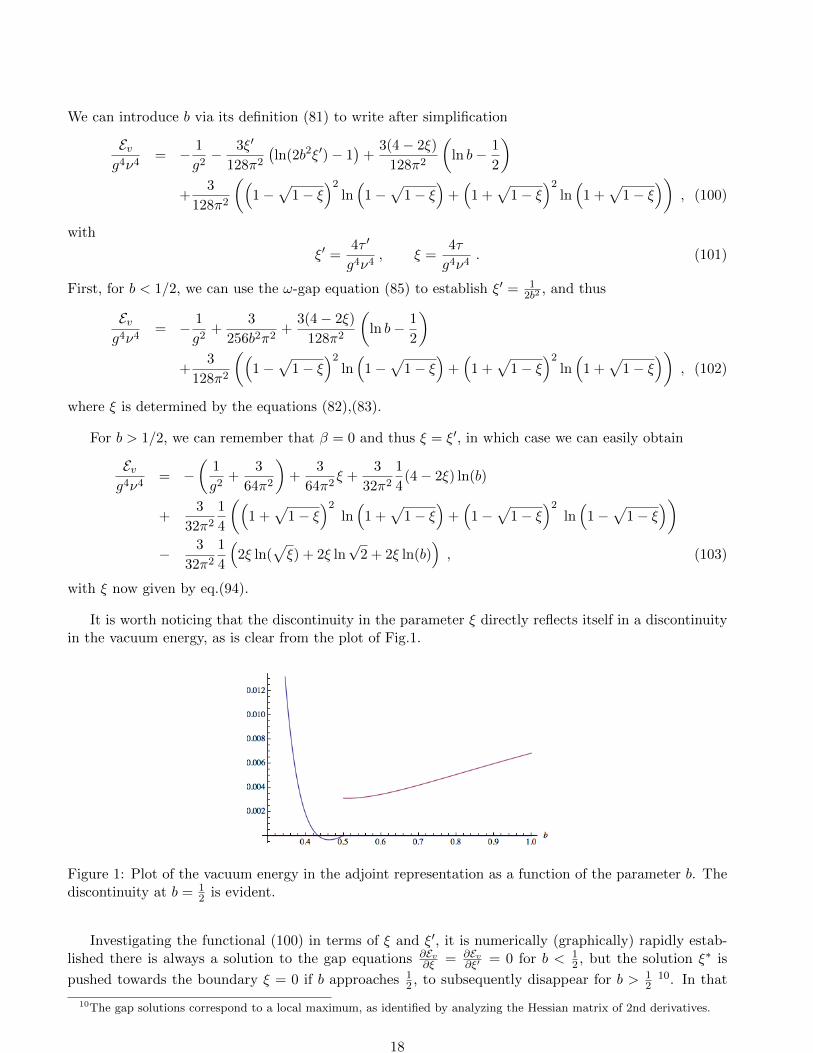
It is worth noticing that the discontinuity in the parameter ξ directly reflects itself in a discontinuityin the vacuum energy, as is clear from the plot of Fig.1.

Figure 1: Plot of the vacuum energy in the adjoint representation as a function of the parameter b. Thediscontinuity at b = 1

2 is evident.

Investigating the functional (100) in terms of ξ and ξ′, it is numerically (graphically) rapidly estab-lished there is always a solution to the gap equations ∂Ev

∂ξ = ∂Ev∂ξ′ = 0 for b < 1

2 , but the solution ξ∗ is

pushed towards the boundary ξ = 0 if b approaches 12 , to subsequently disappear for b > 1

210. In that

10The gap solutions correspond to a local maximum, as identified by analyzing the Hessian matrix of 2nd derivatives.

18

case, we are forced to return on our steps as in the fundamental case and conclude that β = 0, leavingus with a single variable ξ = ξ′ and a new vacuum functional to extremize. There is a priori no reasonwhy these 2 intrinsically different vacuum functionals would be smoothly joined at b = 1

2 . This situationis clearly different from what happens when a potential has e.g. 2 different local minima with differentenergy, where at a first order transition the two minima both become global minima, thereafter changingtheir role of local vs. global. Evidently, the vacuum energy does not jump since it is by definition equalat the transition.

Nevertheless, a completely analogous analysis as for the fundamental case will learn that b = 12 is

beyond the range of validity of our approximation11. The small and large b results can again be shown tobe valid, so at large b (∼ large Higgs condensate) we have a mixture of off-diagonal Yukawa and confineddiagonal modes and at small b (∼ small Higgs condensate) we are in a confined phase. In any case wehave that the diagonal gauge boson is not Coulomb-like, its infrared behaviour is suppressed as it feelsthe presence of the Gribov horizon.

4 Conclusion

In this work we have attempted at studying the transition between the Higgs and the confinement phasewithin a continuum quantum field theory. The problem has been addressed by restricting the domainof integration in the functional integral to the so called Gribov region Ω, which enables us to take intoaccount the nonperturbative effect of the Gribov copies. This framework allows us to discuss the transitionbetween the Higgs phase and the confinement phase by looking at the pole structure of the two-pointgluon correlation function. Both fundamental and adjoint representation for the Higgs field have beenconsidered. The output of our investigation reveals that the case of the fundamental representation isdifferent from that of the adjoint representation, a feature in agreement with the results of numericallattice simulations [1, 2, 3, 4, 5, 6, 7, 8, 9].

In the case of the fundamental representation, the gluon propagator evolves in a continuous way froma confining propagator of the Gribov type to a Yukawa type propagator describing the Higgs phase.Again, this feature is in qualitative agreement with lattice results [1, 2, 3, 4, 5, 6, 7, 8, 9], which showthat the transition between the Higgs and the confining phase occurs in a continuous way. Moreover, wehave been able to show that, in the weak coupling region, i.e. in the Higgs phase, there is no need toimplement the restriction to the Gribov region Ω. Said otherwise, in this region, the presence of the Higgsfield automatically ensures that the theory lies within the Gribov region, so that the Gribov horizon isnot crossed. This is a relevant result, implying that, at weak coupling, the usual Higgs mechanism takesplace, being not affected by the existence of the Gribov copies. A safely asymptotic non-confining theorycan be introduced, with massive gauge bosons as asymptotic states.

In the adjoint representation things look quite different. Besides the confining phase, in which thegluon propagator is of the Gribov type, our results indicate the existence of what can be called a U(1)confining phase for finite values of the Higgs condensate. This is a phase in which the third component A3

µ

of the gauge field displays a propagator of the Gribov type, while the remaining off-diagonal componentsAαµ, α = 1, 2, exhibit a propagator of the Yukawa type. Interestingly, this phase has been already detectedin the lattice studies of the three dimensional Georgi-Glashow model [22, 23]. A second result of ouranalysis is the absence of the Coulomb phase for finite Higgs condensate. For an infinite value of the

11A little more care is needed as the appearance of two Gribov scales complicate the log structure. However, for small bthe Gribov masses will dominate over the Higgs condensate and we can take µ of the order of the Gribov masses to controlthe logs and get a small coupling. For large b, we have β∗ = 0 and a small ω∗: the first log will be kept small by its prefactorand the other logs can be managed by taking µ of the order of the Higgs condensate.

19

latter, we were able to clearly reveal the existence of a massless photon, in agreement with the latticesuggestion of [24].

Summarizing, it seems safe to state that the results we have obtained so far can be regarded as beingin qualitative agreement with the lattice findings and worth to be pursued. Let us end by giving apreliminary list of points for future investigation:

• in the pure gauge case, it has been shown in past years that the Gribov theory dynamically correctsitself via the condensation of the auxiliary fields arising when the restriction to the Gribov regionis implemented in a local and renormalizable way. This has led to the Refined Gribov-Zwanziger(RGZ) theory [31, 32, 33, 34], resulting in propagators and dynamics in very good agreement withlattice investigations [35, 36, 37, 38]. It would be worth to discuss the transition between the Higgsand confining phase within the RGZ framework. This might give more reliable quantitative resultsto be compared with the lattice data.

• within the present approximation, we were not able to address in a concrete and detailed waythe issue of the characterization of the phase diagram in the (ν, g) plane. To that aim, it mightbe interesting to embed in our framework the Polyakov loop P as order parameter of the Higgs-confinement transition, as studied in [6]. In [39], the pure gauge thermodynamics at finite Twas investigated by using the RGZ gluon and ghost propagators. In particular, an approximateeffective action for 〈P〉 was constructed. We can try to couple 〈P〉 to the Gribov effective actionand investigate the interplay of both Gribov mass and 〈P〉 in terms of a varying Higgs condensateg2ν2, the latter quantity playing the role of temperature as in [39].

• certainly, the extension of the present investigation to the case of the gauge group SU(2)×U(1) [40]has an apparent interest, due to its relationship with the electroweak theory. Since the latter is basedon a fundamental Higgs and since we have shown in this paper that in the “perturbative regime”(sufficiently large Higgs condensate and small effective coupling constant) in the fundamental casethe Gribov dynamics becomes trivial, we can expect to recover at least a massless photon for theQED part of the SU(2)× U(1) gauge theory in the same region of (physically relevant) parameterspace. Our preliminary findings [40] do support this naive extrapolation of the here presented work.The concrete analysis is however rather cumbersome, details are thus to be reported at a later stagein [40].

• finally, we hope that our results will motivate further lattice investigations on the behavior of thegluon and ghost propagators in presence of Higgs fields. Although these studies have been alreadystarted in the case of the fundamental representation [7, 8], it would be quite interesting to have atour disposal also data for the case of the adjoint representation.

Acknowledgments

The Conselho Nacional de Desenvolvimento Cientıfico e Tecnologico (CNPq-Brazil), the Faperj, Fundacaode Amparo a Pesquisa do Estado do Rio de Janeiro, the Latin American Center for Physics (CLAF), theSR2-UERJ, the Coordenacao de Aperfeicoamento de Pessoal de Nıvel Superior (CAPES) are gratefullyacknowledged. D. D. is supported by the Research-Foundation Flanders. We thank S. Olejnık fordiscussions.

20

References

[1] E. H. Fradkin and S. H. Shenker, Phys. Rev. D 19 (1979) 3682.

[2] C. B. Lang, C. Rebbi and M. Virasoro, Phys. Lett. B 104 (1981) 294.

[3] W. Langguth, I. Montvay and P. Weisz, Nucl. Phys. B 277 (1986) 11.

[4] V. Azcoiti, G. Di Carlo, A. F. Grillo, A. Cruz and A. Tarancon, Phys. Lett. B 200 (1988) 529.

[5] W. Caudy and J. Greensite, Phys. Rev. D 78 (2008) 025018 [arXiv:0712.0999 [hep-lat]].

[6] C. Bonati, G. Cossu, M. D’Elia and A. Di Giacomo, Nucl. Phys. B 828 (2010) 390 [arXiv:0911.1721[hep-lat]].

[7] A. Maas, Eur. Phys. J. C 71 (2011) 1548 [arXiv:1007.0729 [hep-lat]].

[8] A. Maas and T. Mufti, arXiv:1211.5301 [hep-lat].

[9] J. Greensite, Lect. Notes Phys. 821 (2011) 1.

[10] A. M. Horowitz, Nucl. Phys. B 235 (1984) 563.

[11] P. H. Damgaard and U. M. Heller, Phys. Lett. B 164 (1985) 121.

[12] R. Baier and H. J. Reusch, Nucl. Phys. B 285 (1987) 535.

[13] L. Fister, R. Alkofer and K. Schwenzer, Phys. Lett. B 688 (2010) 237 [arXiv:1003.1668 [hep-th]].

[14] V. Macher, A. Maas and R. Alkofer, Int. J. Mod. Phys. A 27 (2012) 1250098 [arXiv:1106.5381[hep-ph]].

[15] K. Osterwalder and E. Seiler, Annals Phys. 110 (1978) 440.

[16] T. D. Lee and C. N. Yang, Phys. Rev. 87 (1952) 410.

[17] Z. Nussinov, Phys. Rev. D 72 (2005) 054509. [cond-mat/0411163].

[18] V. N. Gribov, Nucl. Phys. B 139 (1978) 1.

[19] R. F. Sobreiro and S. P. Sorella, arXiv:hep-th/0504095.

[20] N. Vandersickel and D. Zwanziger, Phys. Rept. 520 (2012) 175 [arXiv:1202.1491 [hep-th]].

[21] M. A. L. Capri, D. Dudal, A. J. Gomez, M. S. Guimaraes, I. F. Justo and S. P. Sorella,arXiv:1210.4734 [hep-th].

[22] S. Nadkarni, Nucl. Phys. B 334 (1990) 559.

[23] A. Hart, O. Philipsen, J. D. Stack and M. Teper, Phys. Lett. B 396 (1997) 217 [hep-lat/9612021].

[24] R. C. Brower, D. A. Kessler, T. Schalk, H. Levine and M. Nauenberg, Phys. Rev. D 25 (1982) 3319.

[25] J. Greensite, S. Olejnik and D. Zwanziger, Phys. Rev. D 69 (2004) 074506 [hep-lat/0401003].

[26] D. Dudal, S. P. Sorella and N. Vandersickel, Eur. Phys. J. C 68 (2010) 283 [arXiv:1001.3103 [hep-th]].

[27] D. J. Gross and F. Wilczek, Phys. Rev. D 8 (1973) 3633.

21

[28] A. G. M. Pickering, J. A. Gracey and D. R. T. Jones, Phys. Lett. B 510 (2001) 347 [Erratum-ibid.B 535, 377 (2002)] [hep-ph/0104247].

[29] D. Dudal and S. P. Sorella, Phys. Rev. D 86 (2012) 045005 [arXiv:1205.3934 [hep-th]].

[30] F. Lenz, J. W. Negele, L. O’Raifeartaigh and M. Thies, Annals Phys. 285 (2000) 25 [hep-th/0004200].

[31] D. Dudal, S. P. Sorella, N. Vandersickel and H. Verschelde, Phys. Rev. D 77 (2008) 071501[arXiv:0711.4496 [hep-th]].

[32] D. Dudal, J. A. Gracey, S. P. Sorella, N. Vandersickel and H. Verschelde, Phys. Rev. D 78 (2008)065047 [arXiv:0806.4348 [hep-th]].

[33] D. Dudal, S. P. Sorella and N. Vandersickel, Phys. Rev. D 84 (2011) 065039 [arXiv:1105.3371 [hep-th]].

[34] J. A. Gracey, Phys. Rev. D 82 (2010) 085032 [arXiv:1009.3889 [hep-th]].

[35] D. Dudal, O. Oliveira and N. Vandersickel, Phys. Rev. D 81 (2010) 074505 [arXiv:1002.2374 [hep-lat]].

[36] A. Cucchieri, D. Dudal, T. Mendes and N. Vandersickel, Phys. Rev. D 85 (2012) 094513[arXiv:1111.2327 [hep-lat]].

[37] O. Oliveira and P. J. Silva, arXiv:1207.3029 [hep-lat].

[38] D. Dudal, O. Oliveira and J. Rodriguez-Quintero, Phys. Rev. D 86 (2012) 105005 [arXiv:1207.5118[hep-ph]].

[39] K. Fukushima and K. Kashiwa, arXiv:1206.0685 [hep-ph].

[40] M. Capri et al., work in progress.

22