Nuclear Physics B362 (1991) 487-497 North-Holland

EVIDENCE FOR THE EXISTENCE OF GRIBOV COPIES IN LANDAU G A U G E L A T I ' I C E QCD

Enzo MARINARI

Dipartimento di Fisica, Uni~'ersith di Roma, Tor Vergata, Via E. Carnevale, 00173 Rome, Italy and

INFN, Sezione di Roma, Tor Vergata, Rome, Italy

Claudio PARRINELLO

Physics Department, New York Uni~,ersity, 4 Washington Place, New York, NY 10003, USA

Roberto RICCI

Dipartimento di Fisica, Universith di Roma, Tor Vergata, Via E. Carnevale, 00173 Rome, Italy and

INFN, Sezione di Roma, Tor Vergata, Rome, Italy

Received 4 January 1991 (revised 24 April 1991)

We unambiguously show the existence of Gribov copies in a pure SU(3) gauge lattice model, with Wilson action. We show that the usual steepest-descent algorithms used for implementing the lattice Landau gauge lead to ambiguities, which are related to the existence of Gribov copies in the model,

I. Introduction

In 1978 Gr ibov [1] p o i n t e d out tha t in the case of nona be l i a n gauge theor ies the

usual a s sumpt ion of un iqueness of the gauge t r ans fo rmat ions which re la te differ-

ent gauge condi t ions does not necessar i ly hold. In fact when trying to impose the

most p o p u l a r gauge condi t ions (e.g. Cou lomb or Landau) , one can f ind mul t ip le

conf igura t ions of the gauge po ten t i a l s which satisfy the gauge condi t ion . Such

conf igura t ions a re r e l a t ed to each o t h e r by nontr iv ia l gauge t rans format ions .

Such a d r awback does not affect the pe r tu rba t ive approach , s ince the so-cal led

Gribov copies a p p e a r for f ini te va lues o f the gauge field, bu t in view of n o n p e r t u r -

bat ive quan t i za t ion of the theory, they are po ten t i a l ly very dangerous . The i r

0550-3213/91/$03.50 © 1991 - Elsevier Science Publishers B.V. (North-Holland)

488 E. Marinari et al. / Gribot' copies

existence implies that imposing one of the above gauge constraints is not sufficient to remove all the degrees of freedom associated to the group of gauge transforma- tions, and does not allow to identify a fundamental modular region.

Lattice regularization is the best-loved nonperturbative regularization of non- abelian gauge theories, and the possible existence of Gribov copies (that have been first revealed in the continuum formulation) could play here a very important r61e. We will consider here the lattice in Landau gauge, and we will present numerical results that establish the existence of copies in the standard lattice implementation of the Landau gauge. We will argue, in the limit of a small size, small statistics, preliminary analysis, that such copies tend to be stable in the large volume and small lattice spacing limit, so that although they are lattice copies, they seem to be related to the continuum ambiguity.

There are three main points awaiting clarification from results about the lattice Gribov copies. First the definition itself of the nonperturbative theory [2], second the possibility of studying gauge-dependent quantities in the lattice approach, and third the possibility of performing numerical simulations based on algorithms

which need continuity in field space [3]. (i) The first problem is the one originally pointed out by Gribov, and ignored

because of the perturbative nature of the continuum formulation of gauge theo- ries. In a nonperturbative formulation, on the contrary, one has to keep control also of the region of large fields. Functional integration can be used to define the theory if we can pick out the physical configuration space of the theory (see point (ii) about the importance of such a procedure also for the lattice gauge theory).

(ii) The second important point has to do with measuring non gauge-invariant quantities. Indeed, lattice QCD with Wilson action is based on a compact gauge group, and gauge fixing is not compulsory in the course of the Monte Carlo dynamics which allows the determination of gauge-invariant quantities. In this case the gauge-fixing problem is irrelevant in itself, since the gauge degrees of freedom average to zero at large Monte Carlo times. The Gribov problem comes when we want to measure quantities that need gauge fixing, or if we want to implement gauge fixing in order to get more accurate results or to fight, for example, the errors of order a (the lattice spacing). The appearance of Gribov copies in a gauge of interest for the study of gauge-dependent quantities could indeed bring concep- tual difficulties in the interpretation of numerical results, since we would not know which weight the copies should carry in the path integral.

(iii) The third point is related to the use of algorithms in which the continuity of the trajectory is crucial (Langevin equation is the typical approach that can be used, see for example ref. [3] for the SU(2) gauge theory). Imagine you are at step n of the discretized version of an updating continuous algorithm (you are starting from a continuous Langevin-like equation, and you are integrating it with small steps), and you fix the lattice Landau gauge by means of a steepest-descent algorithm. When you perform step n + 1, and fix the gauge again, it could happen

E. Marinari et al. / Gribov copies 489

that the system falls in a different Gribov copy of the system, loosing the continuity

of the time evolution you were interested in. We think that the problem is relevant enough to deserve a systematical analysis,

which we start in this paper. Here we establish the existence of Gribov copies, and we just start a systematic taxonomy of such copies and a study of the continuum limit of the lattice theory. Work along similar lines can be found in ref. [4].

In sect. 2 we discuss the Landau gauge fixing on the lattice. In sect. 3 we draw an analogy with the spin glass theory, where the problem of the existence of many

ground states has received much attention [5, 6]. In sect. 4 we discuss our method to look for Gribov copies. In sect. 5 we discuss our results and in sect. 6 we present

our conclusions.

2. Landau gauge on the lattice

We will define our lattice theory by using the standard Wilson action

-- - y::,,, (n P

where the sum runs over all the plaquettes of the four-dimensional euclidean

lattice,

Je- Re(J~(n)J~(n + ~)J~(n + ~)J,,t(n)), (2)

and the gauge fields take values in the gauge group

Ju(n) e G = S U(3 ) . (3)

The continuum gauge fields A u ( n ) are obtained as

J~,( n) = e iuaA~('' . (4)

It is important here to recall that such a formulation possesses a gauge symmetry that is exactly implemented on the lattice for all values of the lattice spacing a. Given the field o'(n) E G defined on sites (the field of gauge transformations), we

define the transformation

J~,( n ) --* J ~ ) ( n ) = t r (n)J~ , ( n ) t r t ( n + ~z) . (5)

The Wilson action (2) is invariant under transformation (5), as are all closed paths obtained by multiplying the oriented link variables J that one encounters on the path. Closed paths correspond to gauge-invariant observables.

490 E. Marinari et al. / Gribot' copies

As we already said, in the lattice approach in many situations one can avoid gauge fixing. We produce our configurations of gauge fields {J,,(n)} using a Monte Carlo algorithm without fixing the gauge. We select from the stochastic chain configurations that can be considered as independent for practical purposes (i.e.

we perform a large number of Monte Carlo steps before selecting the next configuration for the analysis), and we gauge fix such configurations to the Landau gauge. In order to fix such a gauge we consider the function

V 4

L s [ ~ r ] - - Y', E Re(TrJ~('~)(n)) (6) n = l /*=1

where V is the number of sites which form our euclidean four-dimensional hypercubic lattice.

In terms of the continuum potential (4) we find that, for small g,

A~, (n ) = 2iag ' (7)

where we take for A~, the traceless part. It is easy to yerify that if we choose a

transformed potential {A~)(n)} such that L/(m[o'] is a miflimum for ~r = 1, then the lattice version of

= o ( 8 )

holds. In other words, if Lj[o~] is stationary at each site with respect to small gauge transformations, then the discretized Landau gauge condition holds. We will define a steepest-descent minimization algorithm in order to minimize (6): if it converges, the fixed point will be a Landau gauge-fixed configuration of links. It should be remarked that every stationary point of (6) satisfies eq. (8), so that minimizing (6) corresponds to a gauge-fixing condition somewhat stronger than

(8) (see ref. [7]).

3. A sophisticated spin glass

In sect. 2 we have used quite an unusual notation, which was meant to stress the similarities of our problem with the problem of finding the ground state of a spin glass. Let us underscore here this similarity. The gauge fields Ju can be identified with some link-dependent coupling constant. They are, as usual in spin glass theory, random variables. In this case they are not, as customary, equilibrated according to a gaussian measure, but have been brought to equilibrium according

E. Marinari et al. / Gribov copies

tO the Wilson plaquette Boltzmann weight

491

oCxp[ (9)

Now gauge fixing means considering some spin variable ~r(n) (we are considering an SU(3) spin glass), and finding the ground state of the usual action of a spin model

- Z R e ( T r ( r ( n l J ~ ( n ) q * ( n + / 2 ) ) . (10) ~,.~

The seminal book by Mezard et al. is a very good introduction to the subject [5]. Let us remark here that from this point of view it is absolutely plausible and

natural to find a large number of local minima. We have a strongly disordered system, and the question is whether we have a spin glass phase with different minima of the energy separated, in the infinite-volume limit, by infinite energy barriers. We emphasize that the gauge-fixing procedure we have defined only consists in finding a local minimum of the (spin glass) action, and we never try to reach the global minimum (that would very plausibly take an exponentially large time in the infinite-volume limit).

Clearly, what is crucial is the kind of landscape that the {J} form. For example the deconfined phase could give rise to a behaviour very different from the one observed in the confined phase (where the {J} build up an effective confining potential).

4. Search for copies

We have said that we want to establish whether there exist multiple Gribov copies, i.e. whether there are different local minima of the functional (6).

The first step of the procedure consists in producing a thermalized SU(3) gauge field configuration via a quasi heat-bath [8] Monte Carlo algorithm, at a given value of the lattice volume V and of the inverse squared coupling constant

= g - 2 . We save such a configuration, naming it {M1}.

Next we transform this configuration into the Landau gauge as defined in sect. 3, using a steepest-descent algorithm. As in ref. [9], to control the approach to the Landau gauge we monitor two quantities: one is

24V ' (11)

that is the quantity we are minimizing site by site, and which decreases monotonously. The other one, called O, is a lattice analogue of the squared norm

492 E. Marinari et al. / Gribov copies

of the four-divergence of A . We define

and

We monitor

A(n)- E(Au(n)-A~(n-/x)) (12) tt

O( n) - T r [ A ( n ) A * ( n ) ] (13)

2o0(n) 0= (14)

Obviously we expect a decrease of 0 (not necessarily monotonic) towards 0.

We have checked stability of our runs versus the use of single or double precision arithmetics. First we have done some runs in single precision, that we have repeated in double precision, getting compatible results. Eventually we have used double precision for all our minimization runs. The minimization algorithm converges well within the limit of 64-bit arithmetics: typically, when 0 is reduced to

the order of 10-16, Lj has reached a stable value apart from oscillations on the last digit, due to rounding errors. So when 0 gets reduced to 4 × 10- ~6 we save the

current gauge-fixed field configuration (called {G1}) and assume that it has been Landau-gauge fixed.

The next step is to recall the initial Monte Carlo configuration {M1}, which had been saved, and perform on it a series of random gauge transformations (usually 40), in order to obtain a new configuration {M2}, that is a gauge transform of {MI}. Configuration {M 2} becomes the starting point of a new gauge-fixing process; when

0 ~< 4 × 10- i, we save {G 2} and go back to {M 2} to obtain {M 3} via random gauge transformations, and so on.

In this way we obtain {M2}, {M3},..., {MN} a s steps of a sort of random walk in the space of configurations which are gauge transforms of {M 0. If Gribov copies in the Landau gauge exist, configurations {G0,{G 2} . . . . . {GN} , which we have ob- tained via the Landau gauge minimization algorithm, may represent different Gribov copies. The number of each kind of copy we will get will be proportional to the basin of attraction of the specified local minimum (i.e. Gribov copy). Starting from a different position in gauge phase space will potentially lead to different local minima: the number of times a given random start will lead to a given minimum will be connected to the basin of the attraction of the given minimum. We will call the set of configurations {Gt}, {G 2} . . . . . {G N} the gauge-fixed ensem-

ble. As a consistency check we evaluate the Wilson action of all configurations {M i}

and {Gi} , which has to remain constant under the gauge transformation. The value turns out to be stable within the required precision.

E. Marinari et al. / Gribov copies 4 9 3

We consider in turn different configurations from the (non gauge-fixed) Monte

Carlo run (independent configurations, that are separated from a large enough number of quasi heat-bath Monte Carlo steps). At a given value of /3 and V we generate a large set of configurations that we use as a seed for the procedure described above. Such a procedure allows a systematic study of the main features of the Gribov copies (separation of the copies, basin of attraction, etc.). In the language of spin glasses we are interested in measuring averages over the distribu- tion of the J-couplings (gauge fields).

The analysis of the various gauge-fixed ensembles is a crucial step. At first we look at the distribution of the values of Lj associated to the {G~}. We want to recognize configurations which are related by global gauge transformations, since they do not represent different Gribov copies. We have to remember that Lj[cr] is invariant under global gauge transformations, where on all sites or(n) = ~r, so that gauge-fixed configurations characterized by different values of Lj cannot be related by global gauge transformations. Their appearance provides evidence for the existence of Gribov copies.

Once we have found evidence of the existence of copies, as a next step in the analysis we consider couples of gauge-fixed configurations, {G i} and {Gj}, and evaluate the following quantity:

1 D(Gi,Gj) = ~ E E ITr[GgAn) - GjAn)] I. (15)

n /z

If {Gi} and {Gj} are related by a global gauge transformation, then D(Gi, Gj) = O. Such a distance D gives us a hint about how different two Gribov copies are. We have checked in many cases that D(Gi, G j) is of order 10 -7 if the two configura- tions represent the same Gribov copy, and of order 10 -2 if they belong to different Gribov copies. This has been an important check for judging the consistency of our data.

During this work we have also done many consistency checks in order to be sure of not getting trapped by numerical artifacts. For example, we took a given configuration {G i} and performed numerically several global gauge transformations on it, obtaining what we call {~'i}. Then we verified that D(Gi, ~i) = O, with a small, well-controlled rounding error.

5. Results

We have run our simulations on a 44 lattice and on a 64 lattice. In order to stay on the right side of the deconfinement phase transition (the confined one), we have kept the/3-values at 5.5 on the smaller lattice and 5.5 and 5.65 on the larger one. In this way we tried to check (in the limits of a very preliminary short run) the

494 E. Marinari et al. / Gribot' copies

TABLE 1

For the four different starting configurations m i we give the minimum value found for the

functional defined in eq. (6) in each gauge-fixed ensemble, the energy of the

starting configuration and the number of copies found. H e r e / 3 = 5.5

M L ) 1in Energy Copies

1 - 0 . 7 7 3 8 4 6 4 0.4946860 5

2 0.7735785 0.5014250 2

3 - 0 . 7 7 5 1 6 6 6 0.5043060 2

4 0.7697624 0.5111210 7

behaviour of the system when increasing the volume and decreasing the physical temperature.

Let us start by discussing the results on the 64 lattices, which are the most relevant. In tables 1 and 2 we give information about the occurrence of copies in the different ensembles. We give the energies of the configurations produced during the Monte Carlo runs, the number of copies we find and the minimum value found for the functional defined in eq. (6).

In tables 3 and 4 we give detailed information about the single copies, and about their basins of attraction.

We definitely find evidence for Gribov copies, and a very interesting landscape. Two typical cases are the one in which we find one of the copies with a large population and the other ones quite marginal (mainly at /3 = 5.5), and, on the opposite side, the one where the different valleys have populations of comparable size (mainly at /3 = 5.65). We should remark that at /3 = 5.65 the lattice of 64 points is perhaps a bit too close to the deconfining transition point (that is in this case roughly at/3 = 5.9), and that some finite-temperature effects could already be present.

The times needed in order to reach the bottom of the valley fluctuate much, and we cannot find any clear correlation to the energy of the ensemble or to the depth

TABI.E 2

As in table 1, but now/3 = 5.65, for seven initial configurations M i

M L rain Energy Copies J

1 - 0 . 8 0 0 5 7 1 0 0.4590950 6

2 - 0.8039896 0.4647500 4

3 - 0.7999458 /).4655440 2

4 - 0.8050010 0.4682410 1

5 - 0.7986821 0.4701600 3

6 - / ) .7990729 0.4703150 1

7 - 0 . 8 0 5 2 7 2 9 0.4704960 1

E. Marinari et al. / Gribov copies

TABLE 3 For all ensembles of gauge-fixed configurations the values found for the functional defined in

eq. (6), the difference from the minimum value in each ensemble, the number of gauge-fixed representatives which fall in the copy, and the typical number of

iterations needed to reach the minimum are given. Here/3 = 5.5

495

M Lj ( L j - L~in)106 Weight Iterations

1 - 0.7738464128 0 5 1250 - 0.7738464129 0 10 1200 - 0.7724592616 1387 1 1750 - 0.7721076356 1739 1 4100 - 0.7718986706 1948 3 1750

2 - 0.7735784983 0 13 750 - 0.7729142159 664 7 1650

3 - 0.7751665734 0 18 1050 - 0.7733805841 1786 2 1400

4 - 0.7697623941 0 8 1400 - 0.7696260944 136 2 5500 - 0.7696230116 139 1 1850 - 0.7695806409 182 1 2950 - 0.7694378856 325 4 1700 - 0.7693764874 386 2 1050 - 0.7692938244 469 2 1150

of the given valley. It somet imes happens that valleys that are character ized by very

similar energy values have a different behaviour as far as equi l ibra t ion t imes are

concerned.

W h e n increasing /3 at fixed 6 4 volume we find that some of the ensembles do

not conta in non-tr ivial copies. The p h e n o m e n o n is consis tent with the rough

scaling behavior we expect in this /3-region (we are not in the scaling region, bu t

here we are just discussing the order of magn i tude of the decrease of the n u m b e r

of copies). The physical volume on the l a rger /3 lattice is smaller than the other

one, and in this case we expect to get less copies. O ne should also be wary of

f in i t e - t empera tu re effects, and to effects due to the pecul iar s t ructure of the

F a d d e e v - P o p o v lattice opera tor (as clarified by Zwanziger in a recent note [10]).

The different copies are reached at different t imes of the r andom gauge

dynamics. Let us start from conf igurat ion {M2}, which is genera ted , after a r a n d o m

gauge t ransformat ion , from the original Mon te Carlo conf igura t ion ({M~}). Let us

say that it will go in the basin called A. Conf igura t ion ({M3}). genera ted after

ano the r series of r andom gauge t ransformat ions will fall in basin B, etc. Basin A

will appear again as an at t ractor of the gauge-fixing dynamics also after many

series of r a n d o m gauge t ransformat ions . This means we are hopefully inspect ing

the most par t of the (gauge) phase space, f inding again and again the same fixed

points (Gribov copies).

496 E. Marinari et al. / Griboc copies

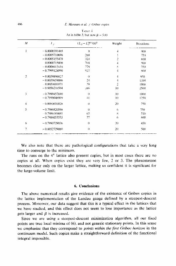
T A m ~ 4

As i n t a b l e 3 , b u t now/3 = 5.65

M Lj ( L j - LI) m~ ) I ( Y ' W e i g h t I t e r a t i o n s

1 - 0.8008391485 I ) 4 900

- 0.8005710696 268 1 750

- 0.8005155470 324 2 600

0.8000715001) 768 4 900

- 0.8000613416 778 5 751)

- 0.7999124890 927 4 900

2 - 0.8039896027 0 4 950

- 0.8039658886 24 4 1 1 0 0

- 0.8039601071 29 2 1000

- 0.80382 1651)4 168 10 2500

3 - 0.7999457690 0 I 0 1000

- 0.7999046909 41 I 0 1251)

4 - 0.8050010028 0 20 751)

5 - 0.7986820588 0 6 75()

- 0.7986188681 63 8 51(1

- I).7986053555 77 6 600

6 - 0.7990729036 0 20 4511

7 - 0.8052729080 1) 21) 500

We also note that there are pathological configurations that take a very long time to converge to the minimum.

The runs on the 4 4 lattice also present copies, but in most cases there are no copies at all. When copies exist they are very few, 2 or 3. The phenomenon becomes clear only on the larger lattice, making us confident it is significant for the large-volume limit.

6. Conclusions

The above numerical results give evidence of the existence of Gribov copies in the lattice implementation of the Landau gauge defined by a steepest-descent process. Moreover, our data suggest that this is a typical effect in the lattices that we have studied, and this effect does not seem to lose importance as the lattice gets larger and /3 is increased.

Since we are using a steepest-descent minimization algorithm, all our fixed points are true local minima of (6), and not generic stationary points. In this sense we emphasize that they correspond to points within the first Gribov horizon in the continuum model. Such copies make a straightforward definition of the functional integral impossible.