1

Polarized Dokshitzer-Gribov-Lipatov- Altarelli-Parisi equations and t-evolution of

structure functions in next-to-leading order at small-x

R.Rajkhowa1, U. Jamil

2 and J.K. Sarma

3

1Physics Department, T.H.B. College, Jamugurihat, Sonitpur, Assam.

2Variable Energy Cyclotron Centre, 1/AF, Bidhan Nagar, Kolkata-64

3Physics Department, Tezpur University, Napaam, Tezpur, Assam.

1E-mail:rasna.rajkhowa@gmail.com

2Email:jamil@veccal.ernet.in

3E-mail:jks@tezu.ernet.in

Abstract

In this paper the spin-dependent singlet and non-singlet structure functions have been

obtained by solving Dokshitzer-Gribov-Lipatov-Altarelli-Parisi evolution equations in next-

to-leading order in the small x limit. Here we have used Taylor series expansion and then the

particular and unique solution to solve the evolution equations. We have also calculated t

evolutions of deuteron, proton and neutron structure functions and the results are compared

with the SLAC E-143 Collaboration data.

PACS No.: 12.38.- t, 12.39.-x, 13.60.Hb, 13.88.+e

Keywords: Unique solution, Particular solution, Complete solution, Altarelli-Parisi equation,

Structure function, Low-x physics.

1. Introduction

DIS of polarized electrons and muons off polarized targets has been used to study the

internal spin structure of the nucleon. The most abundant and accurate experimental

information we have so far comes from the so called longitudinal spin-dependent structure

function g1 which is obtained with longitudinally polarized leptons on longitudinally

polarized protons, deuterons, and 3He targets and it allows separate determination of spin-

dependent deuteron, proton and neutron structure functions [1-8].

In the polarized deep-inelastic scattering (DIS), the spin structure of the nucleon has been

studied by using polarized lepton beams scattered by polarized targets. These fixed-target

experiments have been used to characterize the spin structure of the proton and neutron and

to test additional fundamental QCD and quark-parton model (QPM) sum rules. The first

experiments in polarized electron-polarized proton scattering, performed in the 1970s, helped

establish the parton structure of the proton. In the late 1980s, a polarized muon-polarized

2

proton experiment found that a QPM sum rule was violated, which seemed to indicate that

the quarks do not account for the spin of the proton. This ‘‘proton-spin crisis’’ gave birth to a

new generation of experiments at several high-energy physics laboratories around the world.

The new and extensive data sample collected from these fixed-target experiments has enabled

a careful characterization of the spin dependent parton substructure of the nucleon. The

results have been used to test QCD, to find an independent value for )Q( 2

S , and to probe

with reasonable precision the polarized parton distributions. Recent interest in the spin

structure of the proton, neutron, and deuteron and advances in experimental techniques have

led to a number of experiments concerned with DIS of polarized leptons on various polarized

targets. Among these are the E143 experiments at SLAC [9] and those of the SMC

Collaboration at CERN [10], which used polarized hydrogen and deuterium; the E154

experiment at SLAC [11] and the HERMES Collaboration experiments at DESY [12], which

used polarized 3He; and the HERMES experiment [13], which used polarized hydrogen [14].

A new material, deuterized lithium 6LiD, has recently emerged as a source of polarized

deuterium in the E155/E155x experiments at SLAC [15]. The spin-dependent structure

function g1(x, Q2) for deep-inelastic lepton-nucleon scattering is of fundamental importance

in understanding the quark and gluon spin structure of the proton and neutron. According to

the DGLAP equations [16], g1(x, Q2) is expected to evolve logarithmically with Q

2, where g1

depends both on x, the fractional momentum carried by the struck parton, and on Q2, the

squared four momentum of the exchanged virtual photon. There have been a number of

theoretical approaches [17, 18] to calculate g1(x, Q2) using phenomenological models of

nucleon structure.

The present paper reports particular and unique solutions of polarized DGLAP

evolution equations computed from complete solutions in leading order at low-x and

calculation of t evolutions for singlet, non-singlet, structure functions and hence t-evolutions

of deuteron, proton, neutron structure functions. Here, the integro-differential polarized

DGLAP evolution equations have been converted into first order partial differential equations

by applying Taylor expansion in the small-x limit. Then they have been solved by standard

analytical methods. The results of t-evolutions are compared with the SLAC E-143

Collaboration data.

In the present paper, section 1 is the introduction. In section 2 necessary theory has

been discussed. Section 3 gives results and discussion, and section 4 is conclusion.

3

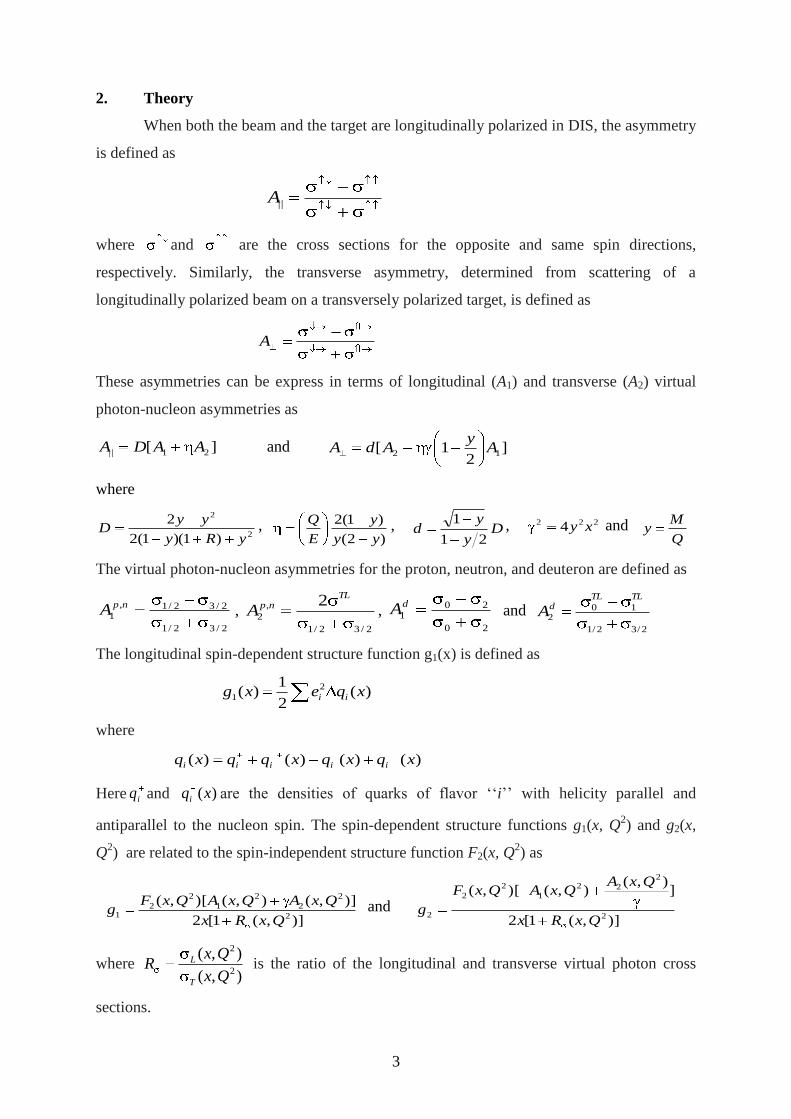
2. Theory

When both the beam and the target are longitudinally polarized in DIS, the asymmetry

is defined as

||A

where and are the cross sections for the opposite and same spin directions,

respectively. Similarly, the transverse asymmetry, determined from scattering of a

longitudinally polarized beam on a transversely polarized target, is defined as

A

These asymmetries can be express in terms of longitudinal (A1) and transverse (A2) virtual

photon-nucleon asymmetries as

][ 21|| AADA and ]2

1[ 12 Ay

AdA

where

2

2

)1)(1(2

2

yRy

yyD ,

)2(

)1(2

yy

y

E

Q , Dy

yd

21

1 , 222 4 xy and Q

My

The virtual photon-nucleon asymmetries for the proton, neutron, and deuteron are defined as

2/32/1

2/32/1,

1

npA , 2/32/1

,

2

2 TLnpA ,

20

201

dA and 2/32/1

102

TLTLdA

The longitudinal spin-dependent structure function g1(x) is defined as

)(2

1)( 2

1 xqexg ii

where

)()()()( xqxqxqqxq iiiii

Here iq and )(xqi are the densities of quarks of flavor ‘‘i’’ with helicity parallel and

antiparallel to the nucleon spin. The spin-dependent structure functions g1(x, Q2) and g2(x,

Q2) are related to the spin-independent structure function F2(x, Q

2) as

)],(1[2

)],(),()[,(2

2

2

2

1

2

21

QxRx

QxAQxAQxFg and

)],(1[2

]),(

),()[,(

2

2

22

1

2

2

2QxRx

QxAQxAQxF

g

where ),(

),(2

2

Qx

QxR

T

L is the ratio of the longitudinal and transverse virtual photon cross

sections.

4

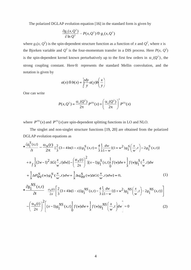
The polarized DGLAP evolution equation [16] in the standard form is given by

),(),(ln

),( 2

1

2

2

2

1 QxgQxPQ

Qxg

where g1(x, Q2) is the spin-dependent structure function as a function of x and Q

2, where x is

the Bjorken variable and Q2 is the four-momentum transfer in a DIS process. Here P(x, Q

2)

is the spin-dependent kernel known perturbatively up to the first few orders in )( 2Qs , the

strong coupling constant. Here represents the standard Mellin convolution, and the

notation is given by

1

0

)()()(y

xbya

y

dyxbxa

One can write

)(2

)()(

2

)(),( )1(

22

)0(2

2 xPQ

xPQ

QxP ss

where )()0( xP and )()1( xP are spin-dependent splitting functions in LO and NLO.

The singlet and non-singlet structure functions [19, 20] are obtained from the polarized

DGLAP evolution equations as

*t

txSg ),(1

2

)(ts 1)},(

12,

1)21{(

13

4),(

1)}1ln(43{

3

2[

xtxSgt

w

xSgww

dwtxSgx

1

0),(

1

1)()(),(

1)1[(

2

2

)(]

1}),(2)12( dwt

w

xSgx

wfdwwftxSgxts

xdwt

w

xGw

fn

,0]1

),(1

)(),(1

)(x

dwtw

xG

xwS

qgqdwtw

xSgwSqqP (1)

*t

txNSg ),(1

2

)(ts1

)},(1

2,1

)21{(13

4),(

1)}1ln(43{

3

2

xtxNSgt

w

xNSgww

dwtxNSgx

01

0

1,

1)()(),(

1)1(

2

2

)(

xdwt

w

xNSgwfdwwftxNSgxts

(2)

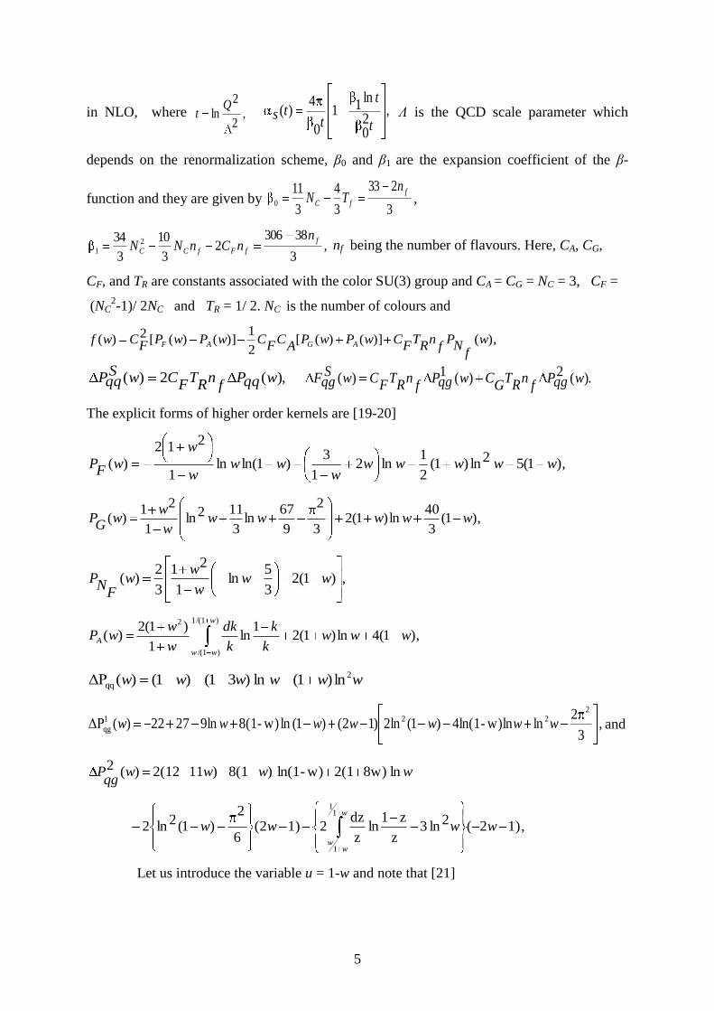
5

in NLO, where ,2

2ln

Qt ,

20

ln11

0

4)(

t

t

tts Λ is the QCD scale parameter which

depends on the renormalization scheme, β0 and β1 are the expansion coefficient of the β-

function and they are given by 3

233

3

4

3

110

f

fC

nTN ,

,3

383062

3

10

3

34 2

1

f

fFfCC

nnCnNN nf being the number of flavours. Here, CA, CG,

CF, and TR are constants associated with the color SU(3) group and CA = CG = NC = 3, CF =

(NC2-1)/ 2NC and TR = 1/ 2. NC is the number of colours and

),()]()([2

1)]()([2)( w

fN

Pf

nR

TF

CwPwPA

CF

CwPwPF

Cwf AGAF

),(2)( wqqPf

nR

TF

CwSqqP ).(2)(1)( wqgP

fn

RT

GCwqgP

fn

RT

FCwS

qgF

The explicit forms of higher order kernels are [19-20]

),1(52ln)1(2

1ln2

1

3)1ln(ln

1

212

)( wwwwww

www

w

wF

P

),1(3

40ln)1(2

3

2

9

67ln

3

112ln1

21)( wwwww

w

ww

GP

,)1(23

5ln

1

21

3

2)( ww

w

ww

FN

P

),1(4ln)1(21

ln1

)1(2)(

)1/(1

)1/(

2

wwwk

k

k

dk

w

wwP

w

ww

A

wwwwww 2

qq ln)1(ln)31()1()(ΔP

,3

2lnw)ln-4ln(1)1(2ln)12()1(lnw)-8(19ln2722)(ΔP

2221

qg wwwwwww and

wwwwqg

P ln8w)2(1w)-ln(1)8(1)112(12)(2

,1)2(2ln3z

z1ln

z

dz21)2(

6

2)1(2ln2

11

1

wwwww

ww

Let us introduce the variable u = 1-w and note that [21]

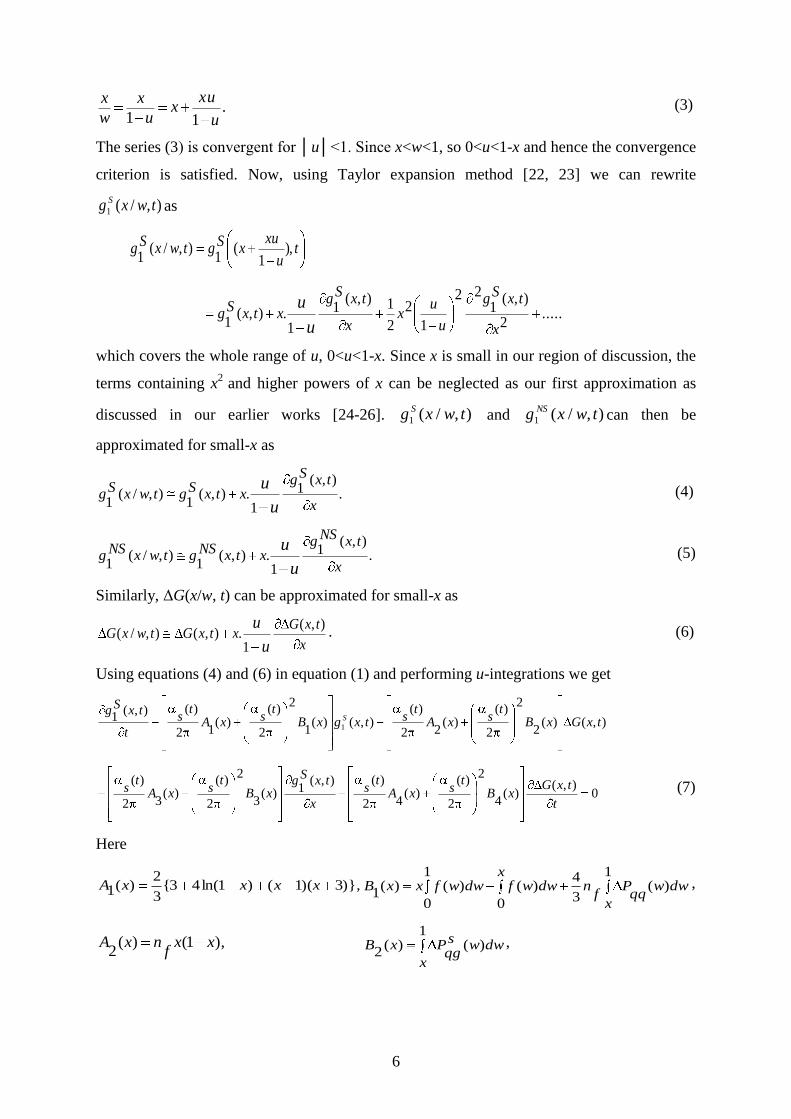
6

.11 u

xux

u

x

w

x (3)

The series (3) is convergent for │u│<1. Since x<w<1, so 0<u<1-x and hence the convergence

criterion is satisfied. Now, using Taylor expansion method [22, 23] we can rewrite

),/(1 twxg Sas

tu

xuxSgtwxSg ),

1(

1),/(

1

.....2

),(1

22

1

2

2

1),(1

1.),(

1x

txSg

u

ux

x

txSgxtxSg

u

u

which covers the whole range of u, 0<u<1-x. Since x is small in our region of discussion, the

terms containing x2

and higher powers of x can be neglected as our first approximation as

discussed in our earlier works [24-26]. ),/(1 twxg S and ),/(1 twxg NS

can then be

approximated for small-x as

.),(

1

1.),(

1),/(

1 x

txSgxtxSgtwxSg

u

u (4)

.),(

1

1.),(

1),/(

1 x

txNSgxtxNSgtwxNSg

u

u (5)

Similarly, ΔG(x/w, t) can be approximated for small-x as

x

txGxtxGtwxG

u

u ),(

1.),(),/( . (6)

Using equations (4) and (6) in equation (1) and performing u-integrations we get

),()(2

2

2

)()(

22

)(),()(

1

2

2

)()(

12

)(),(1

1 txGxBt

sxAt

stxgxBt

sxAt

s

t

txSgS

0),(

)(4

2

2

)()(

42

)(),(1)(

3

2

2

)()(

32

)(

t

txGxB

tsxA

ts

x

txSgxB

tsxA

ts (7)

Here

)},3)(1()1ln(43{3

2)(1 xxxxA

1)(

3

4

0

)(1

0

)()(1

x

dwwqq

Pf

nx

dwwfdwwfxxB ,

),1()(2

xxf

nxA 1

)()(2

x

dwwsqg

PxB ,

7

)},1

ln(2)21({3

2)(3 x

xxxxA 1 1

)(3

4)()(

3x

dww

ww

qqP

fnwfxxB ,

},ln)2)(1{()(4

xxxxf

nxA 1

.)(1

)(4

x

dwwsqg

Pw

wxxB

We assume [24-26, 28]

ΔG(x, t) = K(x) ),(1 txg S. (8)

Here, K is a function of x. It is to be noted that if we consider Regge behaviour of singlet and

gluon structure function, it is possible to solve coupled evolution equations for singlet and

gluon structure functions and evaluate K(x) in LO and NLO. Otherwise this is a parameter to

be estimated from experimental data. We take K(x) = k, axb, ce

-dx, where k, a, b, c, d are

constants. Therefore equations (7) becomes

0),(

1)(2

2

2

)()(

22

)(),()(

1

2

2

)()(

12

)(),(1

1t

txSgxM

tsxL

tstxgxM

tsxL

ts

t

txSgS

(9)

Here,

x

)x(K)x(A)x(A)x(K)x(A)x(L

4211, L2(x) = A3(x) + K(x) A4 (x),

x

xKxBxBxKxBxM

)()(

4)(

2)()(

1)(

1, )(

4)()(

3)(

2xBxKxBxM .

For a possible solution, we assume[25,26] that

,2

)(

0

2

2

)( tsTts (10)

where, T0 is a numerical parameter to be obtained from the particular Q2-range under study.

By a suitable choice of T0 we can reduce the error to a minimum. Now equation (9) can be

recast as

,0),(1

),(),(

1),(),(

1 txSgtxS

Qx

txSgtx

SP

t

txSg (11)

where, )].(20

)(2

[2

)(),( xMTxL

tstxS

P

and )](10

)(1

[2

)(),( xMTxL

tstxS

Q

Secondly using equation (5) and (9) in equation (2) and performing u-integration we have

8

0),(1

),(),(

1),(),(

1 txNSgtxNS

Qx

txNSgtx

NSP

t

txNSg (12)

where )](50

)(5

[2

)(),( xBTxA

tstxNS

P

and

)].(60

)(6

[2

)(),( xBTxA

tstxNS

Q

with,

)},1

ln(2)21({3

2)(

5 xxxxxA ,)(

11)(

5dwwf

x w

wxxB

)},3)(1()1ln(43{3

2)(

6xxxxA

xdwwfxdwwfxB

0

1

0.)()()(

6

The general solution [23, 27] of equation (11) is g (U, V) = 0, where g is an arbitrary function

and U (x, t, Sg1 ) = C1 and V (x, t,

Sg1 ) = C2, where C1 and C2 are constants and they form a

solutions of equations

.),(

),(1

1),( txS

Q

txSdgdt

txS

P

dx (13)

We observed that the Lagrange’s auxiliary system of ordinary differential equations [23, 27]

occurred in the formalism can not be solved without the additional assumption of

linearization (equation (10)) and introduction of an adhoc parameter T0. This parameter does

not effect in the results of t- evolution of structure functions. Solving equation (13) we obtain,

a

xS

N

t

btbtSgtxU

)(exp

)1/()

1,,( and )](exp[),(

1)

1,,( x

SMtxSgSgtxV

where,

,

0

2a ,

20

1b )(

20)(

2

)(xMTxL

dxx

SN and .

)(20

)(2

)(10

)(1

)( dxxMTxL

xMTxLx

SM

2. (a) Complete and Particular Solutions

Since U and V are two independent solutions of equation (13) and if α and β are

arbitrary constants, then V = αU + β may be taken as a complete solution [23, 27] of equation

(11). We take this form as this is the simplest form of a complete solution which contains

9

both the arbitrary constants α and β. Earlier [28] we considered a solution AU + BV = 0,

where A and B are arbitrary constants. But that is not a complete solution having both the

arbitrary constants as this equation can be transformed to the form V = CU, where C=-A/B, i.

e. the equation contains only one arbitrary constant. So, the complete solution

a

xS

N

t

btbtx

SMtxSg

)(exp

)1/()](exp[),(

1 (14)

is a two-parameter family of surfaces, which does not have an envelope, since the arbitrary

constants enter linearly [23,27]. Differentiating equation (14) with respect to β we get 0 = 1,

which is absurd. Hence there is no singular solution. The one parameter family determined by

taking β = α2 has equation

.2)(exp

)1/()](exp[),(

1 a

xS

N

t

btbtx

SMtxSg (15)

Differentiating equation (15) with respect to α, we obtain

.)(

exp)1/(

2

1

a

xS

N

t

btbt

Putting the value of α again in equation (15), we obtain envelope

.

2)(

exp)1/(

4

1)](exp[),(

1 a

xS

N

t

btbtx

SMtxSg

Therefore,

,)()(22

exp)1/(2

4

1),(

1x

SM

a

xS

N

t

btbttxSg (16)

which is merely a particular solution of the general solution.

Now, defining

,)()(2

0

2exp

)10

/(2

04

1)

0,(

1x

SM

a

xS

N

t

btbttxSg

at t = t0, where, t0 = ln (Q02/Λ

2) at any lower value Q = Q0, we get from equation (16)

,

0

112exp

2

)10

/(

0

)1/(

)0

,(1

),(1 tt

btb

t

tbt

txSgtxSg (17)

which gives the t-evolution of singlet structure function ),(1 txg S in NLO.

Proceeding exactly in the same way, and defining

10

,)()(2

0

2exp

)10

/(2

04

1)

0,(1 xM

a

xN

t

btbttxg NS

NSNS

where, )x(5B0

T)x(5A

dx)x(NNS and

dx)x(5B

0T)x(5A

)x(6B0

T)x(6A)x(M NS , we get

for non-singlet structure function in NLO.

0

112exp

2

)10

/(

0

)1/(

)0

,(1

),(1 tt

btb

t

tbt

txNSgtxNSg (18)

which gives the t-evolution of singlet structure function ),(1 txg NS in NLO for β = α2. In an

earlier communication [29], we suggested that for low-x in LO for β = α2

,

2

0),(

1),(

1 0t

ttxSgtxSg (19)

and

.

2

0),(

1),(

1 0t

ttxNSgtxNSg (20)

We observe that if b tends to zero, then eqns. (17) and (18) tend to eqns. (19) and (20) respectively,

i.e., solution of NLO equations goes to that of LO equations. Physically, b tends to zero means that

the number of flavours is high.

Again defining,

,

0

)()(22

exp)1/(

4

1),

0(

1xx

xS

Ma

xS

N

t

btbttxSg

we obtain from equation (16)

,

0)(

20)(

2

)(10

)(1

)(20

)(2

1.

2exp),

0(

1),(

1dx

x

x xMTxL

xMTxL

xMTxLatxSgtxSg (21)

which gives the x-evolution of singlet structure function ),(1 txg Sin NLO.

Similarly defining,

,

0

)()(22

exp)1/(

4

1),

0(1

xxxM

a

xN

t

btbttxg NS

NSNS

we get

11

,

0)(

50)(

5

)(60

)(6

)(50

)(5

1.

2exp),

0(),(

11 dxx

x xBTxA

xBTxA

xBTxAatxgtxg NSNS (22)

which gives the x-evolution of non-singlet structure function ),(1 txg NS in NLO. In an earlier

communication [29], we suggested that for low-x in LO for β = α2

dxx

xxL

xL

xLf

AtxSgtxSg

0)(

2

)(1

)(2

2exp),(

1),(

1 0 (23)

and

,

0)(

)(

)(

2exp),(

1),(

1 0 dxx

xxQ

xP

xQf

AtxNSgtxNSg (24)

For all these particular solutions, we take β = α2. But if we take β = α and differentiate with

respect to α as before, we can not determine the value of α. In general, if we take β = αy, we get in the

solutions, the powers of 1

0

1 0t/bt/b tt and co-efficient of b (1/t-1/to) of exponential part in t-

evolutions and the numerators of the first term inside the integral sign be y/(y-1) for x-evolutions in

NLO. Then if y varies from minimum (=2) to maximum (= ∞) then y/(y-1) varies from 2 to 1.

For phenomenological analysis, we compare our results with various experimental

structure functions. Deuteron, proton and neutron structure functions can be written as

),,(9

5),( 11 txgtxg Sd

(25)

,),(18

3),(

18

5),( 111 txgtxgtxg NSSp

(26)

.),(18

3),(

18

5),( 111 txgtxgtxg NSSn

(27)

Now using equations (17) (18), (21) in equations (25), (26) and (27) we will get t-evolutions

of deuteron, proton, neutron and x-evolution of deuteron structure functions at low-x as

function F2d(x, t) at low-x in NLO as

0

112exp

2

)10

/(

0

)1/(

)0

,(),(,,

1,,

1tt

btb

t

tbt

txgtxgnpdnpd

(28)

and

12

,

0)(

20)(

2

)(10

)(1

)(20

)(2

1.

2exp),

0(),( 11 dx

x

x xMTxL

xMTxL

xMTxLatxgtxg dd (29)

In NLO.

In an earlier communication [29], we suggested that for low-x in LO for β = α2

,

2

0),(

,,1

),(,,

1 0t

ttx

npdgtx

npdg (30)

dxx

xxL

xL

xLf

Atxdgtxdg

0)(

2

)(1

)(2

2exp),(

1),(

1 0 (31)

The determination of x-evolutions of proton and neutron structure functions like that of

deuteron structure function is not suitable by this methodology; because to extract the x-

evolution of proton and neutron structure functions, we are to put equations (21) and (22) in

equations (26) and (27). But as the functions inside the integral sign of equations (21) and

(22) are different, we need to separate the input functions ),( 01 txg S and ),( 01 txg NS

from the data

points to extract the x-evolutions of the proton and neutron structure functions, which may

contain large errors.

2. (b) Unique Solutions

Due to conservation of the electromagnetic current, 1g must vanish as Q2 goes to zero

[30, 31]. Also R→0 in this limit. Here R indicates ratio of longitudinal and transverse cross-

sections of virtual photon in DIS process. This implies that scaling should not be a valid

concept in the region of very low-Q2. The exchanged photon is then almost real and the close

similarity of real photonic and hadronic interactions justifies the use of the Vector Meson

Dominance (VMD) concept [32-33] for the description of F2. In the language of perturbation

theory, this concept is equivalent to a statement that a physical photon spends part of its time

as a ‘bare’, point-like photon and part as a virtual hadron [31]. The power and beauty of

explaining scaling violations with field theoretic methods (i.e., radiative corrections in QCD)

remains, however, unchallenged in as much as they provide us with a framework for the

whole x-region with essentially only one free parameter Λ [34]. For Q2

values much larger

than Λ2, the effective coupling is small and a perturbative description in terms of quarks and

gluons interacting weakly makes sense. For Q2 of order Λ

2, the effective coupling is infinite

and we cannot make such a picture, since quarks and gluons will arrange themselves into

13

strongly bound clusters, namely, hadrons [30] and so the perturbation series breaks down at

small-Q2 [30]. Thus, it can be thought of Λ as marking the boundary between a world of

quasi-free quarks and gluons, and the world of pions, protons, and so on. The value of Λ is

not predicted by the theory; it is a free parameter to be determined from experiment. It should

expect that it is of the order of a typical hadronic mass [30]. Since the value of Λ is so small

we can take at Q = Λ, 0),(1 txg S due to conservation of the electromagnetic current [31].

This dynamical prediction agrees with most adhoc parameterizations and with the data [34].

Using this boundary condition in equation (10) we get β = 0 and

,)()(2

exp)1/(

),(1

xS

Ma

xS

N

t

btbttxSg (32)

Now, defining

,)()(2

0

exp)1

0/(

)0

,(1

xS

Ma

xS

N

t

btbttxSg at t = t0, where t0 = ln (Q0

2/Λ

2) at any lower

value Q = Q0, we get from equations (32)

0

11exp

)10

/(

0

)1/(

)0

,(1

),(1 tt

btb

t

tbt

txSgtxSg (33)

which gives the t-evolutions of singlet structure function ),(1 txg Sin NLO. In an earlier

communication [29], we suggested that for low-x in LO

,0

),(1

),(1 0

t

ttxSgtxSg (34)

and

.

2

0),(

1),(

1 0t

ttxNSgtxNSg (35)

Proceeding in the same way, we get

,

0)(

20)(

2

)(10

)(1

)(20

)(2

1.

1exp),

0(

1),(

1dx

x

x xMTxL

xMTxL

xMTxLatxSgtxSg (36)

which gives the x-evolutions of singlet structure function ),(1 txg Sin NLO.

Similarly, we get for non-singlet structure functions

0

11exp

)10

/(

0

)1/(

)0

,(1

),(1 tt

btb

t

tbt

txNSgtxNSg (37)

14

,

0)(

50)(

5

)(60

)(6

)(50

)(5

1.

1exp),

0(),(

11 dxx

x xBTxA

xBTxA

xBTxAatxgtxg NSNS (38)

which give the t and x-evolutions of non-singlet structure functions ),(1 txg NS in NLO. In an

earlier communication [29], we suggested that for low-x in LO

dxx

xxL

xL

xLf

AtxSgtxSg

0)(

2

)(1

)(2

1exp),(

1),(

1 0 (39)

and

,

0)(

)(

)(

1exp),(

1),(

1 0 dxx

xxQ

xP

xQf

AtxNSgtxNSg (40)

Therefore corresponding results for t-evolution of deuteron, proton, neutron structure

functions and x-evolution of deuteron structure function are

0

11exp

)10

/(

0

)1/(

)0

,(,,

1),(

,,1 tt

btb

t

tbt

txnpd

gtxnpd

g (41)

and

,

0)(

20)(

2

)(10

)(1

)(20

)(2

1.

1exp),

0(

1),(

1dx

x

x xMTxL

xMTxL

xMTxLatxdgtxdg (42)

in NLO. In an earlier communication [29], we suggested that the corresponding results for t-

evolution of deuteron, proton, neutron structure functions and x-evolution of deuteron

structure function are

,0

),(,,

1),(

,,1 0

t

ttx

npdgtx

npdg (43)

dxx

xxL

xL

xLf

Atxdgtxdg

0)(

2

)(1

)(2

1exp),(

1),(

1 0 (44)

in LO.

Already we have mentioned that the determination of x-evolutions of proton and neutron

structure functions like that of deuteron structure function is not suitable by this

methodology. It is to be noted that unique solutions of evolution equations of different

structure functions are same with particular solutions for y maximum (y = ∞) in β = αy

15

relation. The procedure we follow is to begin with input distributions inferred from

experiment and to integrate the evolution equations (36) and (38) numerically.

3. Results and Discussion

In the present paper, we have compared the results of t -evolutions of spin-dependent

deuteron, proton and neutron structure functions in LO with different experimental data sets

measured by the SLAC-E-143 [35] collaboration. The SLAC-E-143 collaborations data sets

give the measurement of the spin-dependent structure function of deuteron, proton and

neutron in deep inelastic scattering of spin-dependent electrons at incident energies of 9.7,

16.2 and 29.1 GeV on a spin-dependent Ammonia target. Data cover the kinematical x range

0.024 to 0.75 and Q2-range from 0.5 to 10 GeV

2.

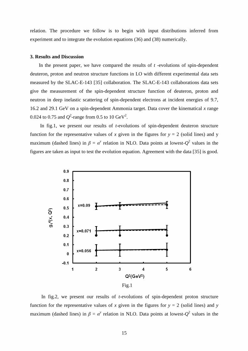
In fig.1, we present our results of t-evolutions of spin-dependent deuteron structure

function for the representative values of x given in the figures for y = 2 (solid lines) and y

maximum (dashed lines) in β = αy relation in NLO. Data points at lowest-Q

2 values in the

figures are taken as input to test the evolution equation. Agreement with the data [35] is good.

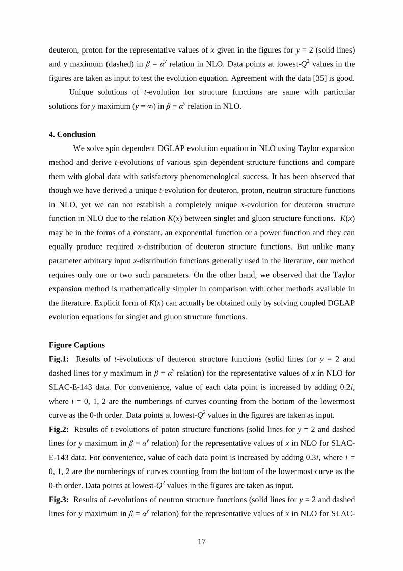
In fig.2, we present our results of t-evolutions of spin-dependent proton structure

function for the representative values of x given in the figures for y = 2 (solid lines) and y

maximum (dashed lines) in β = αy relation in NLO. Data points at lowest-Q

2 values in the

Fig.1

16

figures are taken as input to test the evolution equation. Agreement with the data [35] is

found to be excellent.

Fig.2

Fig.3

In fig.3, we present our results of t-evolutions of spin-dependent neutron structure function

17

deuteron, proton for the representative values of x given in the figures for y = 2 (solid lines)

and y maximum (dashed) in β = αy relation in NLO. Data points at lowest-Q

2 values in the

figures are taken as input to test the evolution equation. Agreement with the data [35] is good.

Unique solutions of t-evolution for structure functions are same with particular

solutions for y maximum (y = ∞) in β = αy relation in NLO.

4. Conclusion

We solve spin dependent DGLAP evolution equation in NLO using Taylor expansion

method and derive t-evolutions of various spin dependent structure functions and compare

them with global data with satisfactory phenomenological success. It has been observed that

though we have derived a unique t-evolution for deuteron, proton, neutron structure functions

in NLO, yet we can not establish a completely unique x-evolution for deuteron structure

function in NLO due to the relation K(x) between singlet and gluon structure functions. K(x)

may be in the forms of a constant, an exponential function or a power function and they can

equally produce required x-distribution of deuteron structure functions. But unlike many

parameter arbitrary input x-distribution functions generally used in the literature, our method

requires only one or two such parameters. On the other hand, we observed that the Taylor

expansion method is mathematically simpler in comparison with other methods available in

the literature. Explicit form of K(x) can actually be obtained only by solving coupled DGLAP

evolution equations for singlet and gluon structure functions.

Figure Captions

Fig.1: Results of t-evolutions of deuteron structure functions (solid lines for y = 2 and

dashed lines for y maximum in β = αy relation) for the representative values of x in NLO for

SLAC-E-143 data. For convenience, value of each data point is increased by adding 0.2i,

where i = 0, 1, 2 are the numberings of curves counting from the bottom of the lowermost

curve as the 0-th order. Data points at lowest-Q2 values in the figures are taken as input.

Fig.2: Results of t-evolutions of poton structure functions (solid lines for y = 2 and dashed

lines for y maximum in β = αy relation) for the representative values of x in NLO for SLAC-

E-143 data. For convenience, value of each data point is increased by adding 0.3i, where i =

0, 1, 2 are the numberings of curves counting from the bottom of the lowermost curve as the

0-th order. Data points at lowest-Q2 values in the figures are taken as input.

Fig.3: Results of t-evolutions of neutron structure functions (solid lines for y = 2 and dashed

lines for y maximum in β = αy relation) for the representative values of x in NLO for SLAC-

18

E-143 data. For convenience, value of each data point is increased by adding 0.3i, where i =

1, 4 are the numberings of curves counting from the bottom of the lowermost curve as the 1st

order. Data points at lowest-Q2 values in the figures are taken as input.

References

1. P. Chiappetta and J. Soffer, Phys. Rev. D 31 (1985) 1019.

2. Bourrely and J. Soffer, Phys. Rev. D 53 (1996) 4067.

3. X. Jiang, G. A. Navarro, R. Sassot, Eur. Phys. J. C 47 (2006) 81.

4. Ziaja, Phys. Rev. D 66 (2002) 114017.

5. K. Abe et. al., Phys. Rev. Lett. 78 (1997) 815.

6. Preparata, P. G. Ratchiffe and J. Soffer, Phys. Rev. D 42 (1990) 930.

7. Adams et. al., Phys. Rev. D 56 (1997) 5330.

8. V. N. Gribov and L. N. Lipatov, Sov. J. Nucl. Phys. 15 (1972) 438; Yu. L. Dokshitzer, Sov.

Phys. JETP 46 (1977) 641.

9. K. Abe et al. (E-143 Collaboration), Phys. Rev. D 58, 112003 (1998).

10. B. Adeva et al. (SMC Collaboration), Phys. Rev. D 58,112001 (1998).

11. K. Abe et al. (E-154 Collaboration), Phys. Lett. B 405,180 (1997); Phys. Rev. Lett. 79, 26

(1997).

12. K. Ackersta et al. (HERMES Collaboration), Phys. Lett. B 404, 383 (1997).

13. A. Airapetian et al. (HERMES Collaboration), Phys. Lett.B 442, 484 (1998).

14. S. Bultmann et al., Report No. SLAC-PUB-7904, 1998.

15. P. L. Anthony et al. (E155 Collaboration), Phys. Lett. B 463, 339 (1999).

16. G. Altarelli, R. D. Ball, and S. Forte, Nucl. Phys. B575, 313 (2000); M. Hirai, S. Kumano,

and Myiama, Comput. Phys. Commun. 108, 38 (1998).

17. A. Cafarella and C. Coriano, Comput. Phys. Commun.160, 213 (2004); J. High Energy Phys.

11 (2003) 059.

18. G. P. Salam and J. Rojo, Comput. Phys. Commun. 180,120 (2009).

19. J. Kwiecinski and B. Ziaja, Phys. Rev. D 60 (1999) 054004.

20. M. Hirai, S. Kumano and Myiama, Comput. Phys. Commun. 108 (1998) 38.

21. I S Granshteyn and I M Ryzhik, ‘Tables of Integrals, Series and Products’, ed. Alen Jeffrey,

Academic Press, New York (1965).

22. S Narayan, ‘A Course of Mathematical Analysis’, S. Chand & Company (Pvt)Ltd., New

Delhi (1987).

23. Ayres Jr., ‘Differential Equations’, Schaum’s Outline Series, McGraw-Hill (1952).

19

24. R Rajkhowa and J K Sarma, Indian J. Phys., 78A (3) (2004) 367.

25. R Rajkhowa and J K Sarma, Indian J. Phys. 78 (9) (2004) 979.

26. R Rajkhowa and J K Sarma, Indian J. Phys. 79 (1) (2005) 55.

27. F H Miller, ‘Partial Differential Equation,’ John and Willey (1960).

28. D K Choudhury and J K Sarma, Pramana--J. Physics. 39, (1992) 273.

29. R Rajkhowa, hep-ph/1002.0623 [2010].

30. F Halzen, A D Martin, ‘Quarks and Leptons: An Introductory Course in Modern Particle

Physics’, John and Wiley (1984).

31. B Badelek et. al, ‘Small-x Physics’, DESY 91-124, October (1991).

32. G Grammer and J D Sullivan, ‘ Electromagnetic Interactions of Hadrons’, eds. A Donnachie

and G Shaw, Plenum Press (1978).

33. T H Bauer et al., Rev. Mod. Phys. 50 (1978) 261.

34. E Reya, ‘Perturbative Quantum Chromodynamics’, DESY 79/88, DO-TH 79/20 (1979).

35. Abe et al., SLAC-PUB-7753 (1998); Phys. Rev. D 58 (1998) 112003.