
Circularly Polarized Antennas for GNSS Applications by ...
181
Circularly Polarized Antennas for GNSS Applications by Umniyyah Ulfa Hussine Thesis submitted in accordance with the requirements for the award of the degree of Doctor of Philosophy of the University of Liverpool January 2021
-
Upload
khangminh22 -
Category
Documents
-
view
1 -
download
0
Transcript of Circularly Polarized Antennas for GNSS Applications by ...
Circularly Polarized Antennas for
GNSS Applications
by
Umniyyah Ulfa Hussine
Thesis submitted in accordance with the requirements for the award of the degree of
Doctor of Philosophy of the University of Liverpool
January 2021

Abstract P a g e | i
Global navigation satellite system (GNSS) is developing rapidly. Modern GNSS
technology is facing challenges for researchers to explore. One hot topic is the multi-
system GNSS device. The motivation for the antenna designers is to miniaturize the
size of the antenna and meanwhile keep its standard performance. It is a challenging
task for an antenna array design to achieve a wide bandwidth, high gain, small size,
good coverage, and simple fabrication technique all at the same time. This thesis
develops several different novel compacts, high gain, and wide bandwidth circularly
polarized (CP) antenna capable of providing wide coverage for GNSS frequency
bands from 1.16 GHz to 1.6 GHz to cover the GPS L1-L5 bands, GLONASS G1,
G2 and G3 as well as the Galileo E5a, E5b, E6, and E1bands.
In the first part of the thesis, the author proposed a new broadband antenna to
cover the GPS L1-L5 bands, GLONASS G1, G2 and G3 as well as the Galileo E5a,
E5b, E6, and E1bands. The antenna is composed of four parasitic elements that are
excited by coupling with the elliptical crossed dipole in the center. By adjusting the
size of the parasitic element and the edge of the dipoles, the coupling strength can be
optimized. The antenna employs a single feed and two orthogonally elliptical printed
dipoles. The dipoles are crossed through a 90° phase delay line of a vacant-quarter
printed ring to achieve CP radiation. The main problem of an antenna equipped with
a metallic reflector is often addressed by including a quarter-wavelength space
between the radiating elements and the reflector to obtain optimal antenna
characteristics. These can be circumvented by using an artificial magnetic conductor

Abstract P a g e | ii
(AMC) surface instead of a metallic reflector. The second contribution is the
development of two novel broadband antennas using two different material of AMC
substrate which is FR-4 and Rogers RT6006. By combining the crossed dipole
radiators and the finite AMC surfaces, low-profile multiband CP antennas that are
nearly completely matched to a single 50 Ω source and have high radiation
efficiencies have been implemented. The proposed antenna has a 10-dB return loss
over 1.153 – 2.36 GHz and achieves a peak realized gain of 5.86 dBi. The interesting
features of the AMC-based crossed dipole antennas are not only their ability to
achieve high efficiency with a low profile but also to generate additional resonances
and the corresponding additional CP radiation features. These were utilized to add
other operating bands or to broaden the antenna bandwidth. Jamming is the act of
intentionally directing electromagnetic energy towards a communication and
navigation system to disrupt or prevent signal transmission. GNSS jammers
broadcast their interference signal in the frequency band used for satellite navigation.
Consequently, the final contribution of the work is a novel wideband CP anti-
jamming antenna array with the capability of generating multiple steerable beam
directions and enables effective jammer suppression with negligible phase distortion.
A 2 × 2 antenna array exhibits a wide bandwidth from 0.995-2.333 GHz and has a
peak gain of 7.6 dBi. In order to have a compact system, a total antenna array
miniaturization has been achieved.
Collectively, these contributions advance the state-of-the-art in GNSS
adaptive antennas in terms of performance, precision, and practicality.

Acknowledgement P a g e | iii
First of all, I thank GOD ALMIGHTY who has given me the mental and physical strength
and confidence to do this work. This thesis would not have seen the light without the support
and guidance of many people who are acknowledged here. I would like to express my deep
gratitude to my supervisor, Professor Yi Huang for offering me this opportunity. His kind
support, fruitful advice, critical discussions, and vast experience have motivated me during
the whole time of my studies. I would also like to thank my second supervisor Dr. Jiafeng
Zhou who has endorsed this life changing opportunity for me.
I would like to offer my personal and special thanks to my husband, Sidek Ismail
and my children, Sarah, Khayra and Rayyan. I would never have succeeded without their
love, tolerance, support, encouragement, and patience. You have always supported me with
no expectation of a reward. Your continuous help and understanding have made my life full
of love and I am grateful for everything you have done. I would also like to express my
appreciation to my parents, Siti Rugayah Tibek and Hussine Hangah and my brother, Farid
Ismat who have encouraged me over the years.
Thanks to all my friends here in Liverpool and also in Malaysia who had been with
me in the very crucial moments of my studies and for boosting my morale. I am very grateful
for all their support and effort to cheer me up.
I would also thank my brilliant and lovely colleagues and friends in the RF group
for many fruitful discussions and enjoyable moments and providing such a lovely
environment for research. Special thanks are also paid to Dr. Chaoyun Song for valuable
advice, contribution, and collaboration in editing the published papers of this research and
for the friendly support. Particular thanks should also be paid to Mark and John from the
Electrical Workshop for always being very kind to me and fabricating my antennas and
circuits very quickly and beautifully. Thanks to Rogers Corporation for providing us with
free samples of PCB boards.
Finally, the financial support from the Ministry of Higher Education Malaysia and
the University of Science Islam Malaysia (USIM) is gratefully acknowledged.

Table of Contents P a g e | iv
1.1 Background 1
1.1.1 Radio Frequency (RF) Performance Parameters of GNSS Antennas 3
1.1.2 GNSS Antenna Fundamentals 10
1.1.3 Design Challenges: Size Constraints, Feed Network, and Cost 19
1.1.4 Basic GNSS Antenna Approaches 21
1.2 Research Motivation and Objectives 24
1.3 Contributions and Organization of This Thesis 25
2.1 Introduction 27
2.1.1 GPS Fundamentals 28
2.1.2 GLONASS Fundamentals 31
2.1.3 Galileo Fundamentals 32
2.1.4 Signal Characteristics 33
2.2 Interference and Jamming 35

Table of Contents P a g e | v
2.2.1 Jamming Attack on GNSS 38
2.2.2 Jamming Effect on GNSS 39
2.3 Anti-Jamming Technique 40
2.3.1 Single Antenna Receiver-based Solutions 40
2.3.2 Antenna Array Based Solutions 41
2.4 Summary 43
3.1 Introduction 44
3.2 GNSS Antenna: Overview 45
3.3 GNSS Crossed-Dipole Antenna 52
3.4 GNSS Adaptive Antenna Arrays 57
3.5 Summary 65
4.1 Introduction 67
4.2 An Antenna with Parasitic Elements 68
4.2.1 Antenna Design Configurations 68
4.2.2 Antenna Performances 71
4.3 Summary 78
5.1 Introduction 80
5.2 Artificial magnetic conductor (AMC) 81
5.2.1 AMC Properties 82
5.3 CP Crossed-Dipole Antenna with AMC Surface on FR-4 Substrate 86
5.3.1 Antenna Design Configurations 86

Table of Contents P a g e | vi
5.3.2 Antenna Performances 90
5.4 CP Crossed-Dipole Antenna with AMC Surface on Rogers RT6006
Substrate 93
5.4.1 Antenna Design Configurations 93
5.4.2 Antenna Performances 96
5.5 Summary 100
6.1 Introduction 102
6.2 Overview of Interference Threat 103
6.3 Circular Polarized Crossed-Dipole Antenna 104
6.3.1 Antenna Element Design 104
6.3.2 Antenna Element Performance 109
6.4 Array Design Configuration 116
6.4.1 Antenna Array Configurations and Performances 118
6.5 Antenna Performances 128
6.6 Summary 133
7.1 Conclusion 136
7.2 Limitation and Future Work 138

List of Tables P a g e | vii
Tables Title Page
Table 1.1: Frequency and Constellations of GNSS Systems 4
Table 1.2: Performance Requirements of a GNSS Antenna Prototype 5
Table 1.3: Basic Antenna Types Used in GNSS and Their General Characteristics
[6] 23
Table 2.1: Classification of Interferences Based on Spectral Characteristics 35
Table 2.2: Types of RF Interference and Their Probable Sources 37
Table 3.1: Basic Antenna Typed Used in GNSS System and Their General
Characteristics 65
Table 4.1: Dimension of The Proposed Antenna 69
Table 4.2: 3 dB Beamwidth of The Proposed Antenna 75
Table 4.3: Comparison with Existing GNSS Antenna Designs 78
Table 5.1: Comparison with Proposed Antenna without AMC 101
Table 6.1: Optimized Parameters of The Proposed Antenna 107
Table 6.2: Dimension of The Proposed Antenna 119
Table 6.3: Dimension of The Proposed Antenna 124
Table 6.4: The Jammer Source Locations in Three Different Scenarios 130

List of Figures P a g e | viii
Figures Title Page
Figure 1.1: GNSS Frequency Bands [6]. 4
Figure 1.2: Ideal antenna gain patterns for GPS antennas (1985–2010) and GNSS
antennas (after 2010) [6]. 7
Figure 1.3: Horizontal and vertical linear polarization [16]. 14
Figure 1.4: Left-handed and Right-handed circular polarization [16]. 15
Figure 2.1: GPS segments. 28
Figure 2.2: Expandable 24-slot satellite constellation. 29
Figure 2.3: Locations of the different sections of the control segment around the
world [34]. 30
Figure 2.4: An RHCP wave where the red spiral traces the RHCP energy, and the
blue and green sinusoidal waves trace the contributions from the x-axis
and y-axis field components. 34
Figure 2.5: Common interference and jamming source. 36
Figure 2.6: Privacy GNSS jammer [40]. 38
Figure 3.1: Geometry of the stacked patch CP antenna (a) side view (b) upper patch
(c) middle patch and (d) lower patch [64]. 45
Figure 3.2: (a) Measured and simulated reflection coefficients of the antenna and
(b) Simulated axial ratio of the proposed antenna [64]. 46
Figure 3.3: The diagram of the hybrid DRA[71]. 48
Figure 3.4: Hybrid DRA performance measured (a) S11 (b) maximum radiation gain
and (c) axial ratio [71]. 49

List of Figures P a g e | ix
Figure 3.5: Fabricated prototype of (a) antenna 1 (b) antenna 2 [59]. 50
Figure 3.6: Simulated and measured (a) reflection coefficient and (b) axial ratio
[59]. 51
Figure 3.7: Geometry of the proposed antenna (a) radiator (b) vacant-quarter
printed ring and dipole arm (c) side view with the inverted pyramidal
cavity [56]. 53
Figure 3.8: Simulated and measured (a) reflection coefficients (b) axial ratios of the
multi-band antenna [56]. 54
Figure 3.9: Geometry of the proposed antenna with a composite cavity [73]. 55
Figure 3.10: (a) Prototype of ultra-wideband composite cavity backed CP antenna
and VSWR and (b) simulated and measured ARs of the antenna with
and without a cavity [73]. 56
Figure 3.11: (a) Prototype using high-contrast substrates and (b) associated
Wilkinson divider for feeding using a single coax feed at Port 1 and (c)
gain of the patch [76]. 58
Figure 3.12: (a) GNSS antenna array design and (b) fabricated prototype [76]. 60
Figure 3.13: Four-element and six-element spiral array [74], [81]. 61
Figure 3.14: (a) Antenna array geometry formed by five identical patch antennas
and (b) radiation pattern at φ = 0° and φ = 90° [82]. 63
Figure 4.1: Geometry of the proposed antenna: (a) top view and (b) side view. 69
Figure 4.2: Vertical radiation patterns for the antennas. (a) elliptical cross-dipole
(b) parasitic element and loaded monopole and (c) crossed dipole
surrounded by parasitic elements and monopoles. 71
Figure 4.3: The simulated S11 with different values of 𝐿𝑔 of the proposed antenna.
72

List of Figures P a g e | x
Figure 4.4: The simulated axial ratio with different values of 𝐿𝑔 of the proposed
antenna. 72
Figure 4.5: The simulated S11 with different values of W of the proposed antenna.
73
Figure 4.6: The simulated axial ratio with different values of W of the proposed
antenna. 73
Figure 4.7: The simulated radiation pattern with and without the parasitic elements
of the proposed antenna at (a) GNSS L2 (b) GNSS L1. 74
Figure 4.8: RHCP radiation patterns in 𝑋𝑜𝑍 and 𝑌𝑜𝑍 planes at 1.575 GHz. 75
Figure 4.9: Photograph of fabricated antenna (a) front view and (b) perspective
view. 76
Figure 4.10: Measured and simulated results of the proposed antenna: |S11|. 77
Figure 4.11: Measured and simulated results of the proposed antenna: AR. 77
Figure 5.1: (a) An array of AMC unit cells with each vias connected to the ground
plane, (b)the equivalent inductance capacitance circuit, and (c)circuit
model [102]. 84
Figure 5.2: Antenna separated (a) closely and (b) further from the ground plane.
(c)Antenna incorporated with AMC is in very close proximity with the
ground layer [86]. 85
Figure 5.3: Geometry of the proposed antenna: (a) top and (b) cross-sectional view
of the proposed antenna. 87
Figure 5.4: Photograph of the fabricated antenna (a),(b) front view and (c) back
view. 89
Figure 5.5: Measured and simulated results of the proposed antenna: |S11|. 90
Figure 5.6: Measured and simulated results of the proposed antenna: AR. 91

List of Figures P a g e | xi
Figure 5.7: Measured and simulated results of the radiation pattern at (a) L1 and (b)
radiation pattern at L2. 92
Figure 5.8: Geometry of the proposed antenna: (a) top and (b) cross-sectional view
of the proposed antenna (c) perspective view. 94
Figure 5.9: Photographs of the fabricated antenna. 95
Figure 5.10: Measured and simulated results of the proposed antenna: |S11|. 97
Figure 5.11: Measured and simulated results of the proposed antenna: AR. 97
Figure 5.12: Measured and simulated radiation pattern results of the proposed
antenna at (a) L5; (b) L2; (c) E6; (d) L1. 99
Figure 6.1: 3D disassembled view of the proposed crossed dipole antenna with
parasitic elements. 105
Figure 6.2: Detailed geometry of the proposed antenna (a) Crossed dipole antenna.
106
Figure 6.3: Evolution of the antenna design: a conventional crossed dipole is
converted to an egg-shaped loop radiator; finally the proposed antenna
is designed with combination elliptical and circle shaped loop radiator.
107
Figure 6.4: Simulated S11 of the reference crossed dipole antenna, the egg-shaped
crossed dipole using loop radiators and the proposed antenna. 108
Figure 6.5: Simulated axial ratio (AR) of the reference crossed dipole antenna, the
egg-shaped crossed dipole using loop radiators and the proposed
antenna. 109
Figure 6.6: Simulated surface current distribution of the proposed antenna with
parasitic element at (a) 1.15 GHz, (b) 1.21 GHz and (c) 1.57 GHz. 110

List of Figures P a g e | xii
Figure 6.7: Simulated 3D radiation pattern of the proposed antenna with parasitic
element at (a) 1.15 GHz. (b) 1.21 GHz. (c) 1.3 GHz. (d) 1.57 GHz. 111
Figure 6.8: The fabricated antenna examples. (a) The crossed dipole at the top of
PCB, (b) the bottom of the antenna, and (c) overall antenna with a
radome. 112
Figure 6.9: Simulated and measured S11 of the proposed antenna. 113
Figure 6.10: Simulated and measured axial ratio of the proposed antenna. 114
Figure 6.11: Simulated and measured radiation pattern over XOZ-plane (left) and
YOZ-plane (right) at three different frequencies. (a) 1.15 GHz. (b) 1.3
GHz. (c) 1.575 GHz. 115
Figure 6.12: Simulated and measured axial ratio of the proposed antenna. 116
Figure 6.13: CRPA unit is receiving satellite and jammer signals. 117
Figure 6.14: Five-element antenna array configurations (a) perspective view (b) top
view and (c) side view of the antenna. 119
Figure 6.15: Array scanning setup for five elements array in CST MWS. 120
Figure 6.16: Simulated reflection coefficients of the proposed antenna. 121
Figure 6.17: Simulated transmission coefficients of the proposed antenna. 121
Figure 6.18: Simulated axial ratio of the proposed antenna. 122
Figure 6.19: Simulated total efficiency of the proposed antenna. 122
Figure 6.20: Simulated realized gain of the proposed antenna. 123
Figure 6.21: Four-element antenna array configurations (a) perspective view (b) top
view and (c) side view of the antenna. 124
Figure 6.22: Array scanning setup for four elements array in CST MWS. 125
Figure 6.23: Simulated reflection coefficient of the proposed antenna. 126
Figure 6.24: Simulated axial ratio of the proposed antenna. 126

List of Figures P a g e | xiii
Figure 6.25: Simulated total efficiency of the proposed antenna. 127
Figure 6.26: Simulated total efficiency of the proposed antenna. 127
Figure 6.27: Antenna array with ideal (point source) and real radiation pattern. 128
Figure 6.28: GPS Antenna array with point sources and real radiation patterns for
SJR=30 dB, SNR=-20 dB and σ = 0.001. The jammer is placed at φj =
90° and θj = 90°. a) φ-plane with θj = 90° b) θ-plane with φj = 90°. 129
Figure 6.29: Array patterns after null steering with SJR = 50 dB for different
jammer locations reported in Table 6.4. 131
Figure 6.30: GPS Antenna with different signal to jammer ratio for SNR = -20 dB
and σ = 0.001. The jammer is placed at 𝜑𝑗 = 45° and 𝜃𝑗= 45° (a) φ-
plane with 𝜃𝑗 = 45° (b) θ-plane with 𝜑𝑗 = 45° 132

List of Acronyms P a g e | xiv
AR Axial Ratio
AMC Artificial Magnetic Conductor
AUT Antenna Under Test
CDMA Code Division Multiple Access
CP Circular Polarization
CS Control Segment
CST Computer Simulation Technology
DC Direct Current
DRA Dielectric Resonator Antenna
EM Electromagnetic
FDMA Frequency Division Multiple Access
FBW Fractional Bandwidth
GEO Geostationary Orbits
GLONASS GLObal Navigation Satellite System
GNSS Global Navigation Satellite Systems
GPS Global Positioning System
HF High Frequency
HIS High Impedance Surface
HPBW Half-Power Beam Width
IEEE Institute of Electrical and Electronics Engineers
IGSO Inclined Geosynchronous Orbits
LF Low Frequency
LHCP Left Hand Circularly Polarized
LNA Low Noise Amplifier
LP Linear Polarization
MEO Medium Earth Orbit
OC Operational Control Segment
PCB Printed Circuit Board

List of Acronyms P a g e | xv
PEC Perfect Electric Conductor
PNT Position, Navigation, and Timing
PPS The Precise Positioning System
PRN Pseudo Random Noise
PVT Position, Velocity, and Timing
QZSS Quasi-Zenith Satellite System
RFI Radio Frequency Interference
RHCP Right Hand Circularly Polarized
RX Receiving Antenna
SAR Specific Absorption Rate
SDR Software-Defined Radio
SIW Substrate Integrated Waveguide
SNR Signal to Noise Ratio
SPS The Standard Positioning Service
SS Space Segment or Satellite Segment
STAP Space-Time Adaptive Processing
SV Satellite Vehicle
TX Transmitting Antenna
UHF Ultra-High Frequency
US User Segment
VSWR Voltage Standing Wave Ratio

List of Publications P a g e | xvi
[1] U. U. Hussine, Y. Huang and C. Song, “A new circularly polarized antenna
for GNSS applications,” in Proc. 2017 11th European Conference on Antennas and
Propagation (EUCAP), 2017, pp. 1–3.
[2] C. Song, Y. Huang and U. U. Hussine, “A broadband circularly polarized
cross-dipole antenna for GNSS applications,” in Proc. 2015 Loughborough Antennas
& Propagation Conference (LAPC), 2015, pp. 1–4.
[3] U. U. Hussine, O. A. Mobayode, Y. Huang and B.Liu, “A novel circularly
polarized antenna for GNSS applications using optimization technique” (to be
submitted)

Chapter 1: Introduction P a g e | 1
CHAPTER 1:
INTRODUCTION
1.1 BACKGROUND
Since the deployment of the Global Positioning System (GPS) by the United States
and a similar GLObal Navigation Satellite System (GLONASS) system by the Soviet
Union around 1990 [1]–[3], GPS applications have proliferated globally, not only in
the military arena but also in commercial and consumer markets. While the
importance of GPS antenna relative to GPS receiver is obvious and remains, the
performance and cost issues have fundamentally changed.
Application of GLONASS has been minuscule after the dissolution of the
Soviet Union. The recent recovery of the Russian economy propelled by the oil boom
has enabled the revitalization of GLONASS, which restarted full constellation
operation in April 2011. In 2002, the European Union started to develop Galileo.

Chapter 1: Introduction P a g e | 2
Originally targeted to start operation in 2008, Galileo suffered from years of delays
due to financial and technical troubles. In 2011, its delayed plan was to have full
global coverage in 2019. China began to develop Compass (Beidou) in the late
1990s, but has been fast moving in recent years, and is positioned to have a full-
fledged Global Navigation Satellites System (GNSS) within a few years [4].
Additionally, GPS, GLONASS, and Compass are also being augmented by
Geostationary Earth Orbit (GEO) satellites to complement their Medium Earth Orbit
(MEO) satellites. Several other countries have also started their regional satellite
navigation systems, such as Japan’s Quasi Zenith Satellite System (QZSS). All these
satellite-based systems constitute the GNSS, with GPS, GLONASS, Galileo, and
Compass being the four cornerstones with global coverage. The upcoming
availability of so many satellites, and over such a wide frequency range, in GNSS
constellations, as well as the move toward more unified code-division multiple-
access (CDMA) approach, in the near future, will offer superior performance and
lower life-cycle cost, as well as new features and capabilities. These game-changing
events are also enabled by newly available low-cost software-defined radio (SDR)
technologies and the unprecedented global economy. To meet the anticipated market
needs, GNSS receivers covering two or more GNSS systems have been developed
and deployed at fairly low costs.
Chapter 1: Introduction P a g e | 3
1.1.1 Radio Frequency (RF) Performance Parameters of GNSS
Antennas
The impact of the fundamental changes from GPS to GNSS has been recognized and
taken advantage of by receiver manufacturers. Several GNSS receivers have recently
shown up in the marketplace, and they can easily adapt to large future changes in
GNSS waveforms since they are based on SDR technology. In the commercial world,
SDR development and application have been growing rapidly since about 2000. On
the other hand, SDR antenna development has not had such success as the receiver.
In this context, RF performance parameters of GNSS receive antennas will be
discussed, highlighting changes from those for conventional GPS.
1.1.1.1 Operating Frequencies and Bandwidths
Table 1.1 displays signals and constellations of the four major GNSS
systems: GPS, GLONASS, Galileo, and Compass, with the data on maximum
bandwidths largely derived from [4] and [5] for interoperability issues. GNSS spectra
are spread densely across 1146 to 1616 MHz, covering a frequency bandwidth of
470 MHz. Obviously, future GNSS antennas will strive to cover more bands and
constellations like antennas driven by the receivers.
Since the receivers will be increasingly more able to cover the entire GNSS
spectrum and take advantage of it, it is desirable and sometimes necessary that their
antennas’ operating frequencies and bandwidths be consistent with those of the
receivers. Additionally, large bandwidths are needed to mitigate detuning due to

Chapter 1: Introduction P a g e | 4
changes in the antenna’s installation environment. In practical applications, there is
also a growing trend for GNSS antennas toward multifunction that covers not only
GNSS but also some satellite communications such as satellite radio, Iridium, etc.
Table 1.1: Frequency and Constellations of GNSS Systems
GPS GLONASS Galileo COMPASS / Beidou
Country USA Russia European
Union China
Constellation 24 MEO 24 MEO 30 MEO
27 MEO
5 GEO
3 IGSO
Coding CDMA FDMA / CDMA CDMA CDMA
Carrier
Frequency
(MHz)
L1:
1575.420
L2:
1227.600
L5:
1176.450
G1: 1602.000 + k
× 0.5625*
G2: 1246.000 + k
× 0.4375*
G3: 1204.704 + k
× 0.4230*
E1: 1575.420
E5a:
1176.450
E5b:
1207.140
E5: 1191.795
E6: 1278.750
B1:
1559.052~1591.788
B2:
1162.220~1217.370
B3:
1250.618~1286.423
Figure 1.1: GNSS Frequency Bands [6].

Chapter 1: Introduction P a g e | 5
These satellite systems are fundamentally similar, and one can typically
develop technology that generally applies to all of them. The research presented in
this work, which focuses on the receiver antenna and its associated signal processing
that applicable to any GNSS system so long as the antenna and antenna electronics
are designed for the required frequencies. In this work, the term “GNSS antenna”
will be frequently used to refer to an antenna designed for any one or multiple
satellite navigation systems. The frequency bands for these GNSS systems and
performance requirements of a GNSS antenna prototype are shown in Figure 1.1 [6]
and Table 1.2 respectively.
Table 1.2: Performance Requirements of a GNSS Antenna Prototype
Parameter Requirement
Resonant Frequency or Operational
Frequency
E1 – E6; L1, L2, L5; G1 – G3; B1 – B3
1.16 to 1.30 GHz and 1.52 to 1.61 GHz
GPS, GLONASS, Galileo and
BeiDou/COMPASS
Bandwidth (VSWR < 2:1) At least 103 MHz on L1 band
Polarization Right Hand Circular Polarization
(RHCP)
Axial Ratio 0 dB to 3-dB at boresight
Gain Variation Less than 15 dB from Zenith to 10°
elevation angle
Zenith Gain Greater than 0 dBic (desired)
Desired to Undesired Ratio (D/U) Minimum 20 dB at 45° Elevation angle

Chapter 1: Introduction P a g e | 6
1.1.1.2 Radiation Pattern and Polarization
Polarization can be defined as the track of the electric field vector for travelling EM
waves. An antenna can be classified as linear polarization (LP), elliptical polarization
(EP) and circular polarization (CP). Right hand circular polarization (RHCP) and
left-hand circular polarization (LHCP) are two types of circular polarization. The
axial ratio (AR) can be defined to measure the level of CP. The AR is 0 dB for a
perfect CP antenna. Usually, when the AR is less than 3 dB, the antenna is a CP
antenna.
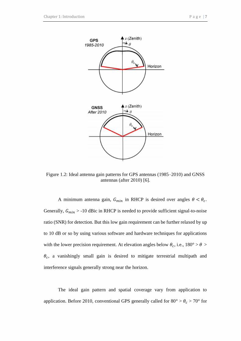
Figure 1.2 depicts two ideal elevation gain patterns, one before and one after
2010, to highlight the fundamental changes. The polar patterns are in spherical and
rectangular coordinates, with the z-axis pointing to the zenith. The gain pattern
optimizes gain and coverage for satellites over 0° ˂ 𝜃 ˂ 𝜃𝑐 and mitigates problems
due to multipath from satellite platform, ionosphere, troposphere, and platform
environment, as well as interferences and noises over 𝜃𝑐 ˂ 𝜃 ˂ 180°. The sharp turn
at elevation “cutoff angle” 𝜃𝑐 is a major design difficulty; a real-world GNSS antenna
generally has a smooth cardioid pattern with hemispherical coverage. 𝜃𝑐 is a crucial
parameter varying between applications but is moving higher toward the zenith with
the advent of GNSS [6].
Chapter 1: Introduction P a g e | 7
Figure 1.2: Ideal antenna gain patterns for GPS antennas (1985–2010) and GNSS
antennas (after 2010) [6].
A minimum antenna gain, 𝐺𝑚𝑖𝑛 in RHCP is desired over angles 𝜃 < 𝜃𝑐 .
Generally, 𝐺𝑚𝑖𝑛 > -10 dBic in RHCP is needed to provide sufficient signal-to-noise
ratio (SNR) for detection. But this low gain requirement can be further relaxed by up
to 10 dB or so by using various software and hardware techniques for applications
with the lower precision requirement. At elevation angles below 𝜃𝑐, i.e., 180° > 𝜃 >
𝜃𝑐, a vanishingly small gain is desired to mitigate terrestrial multipath and
interference signals generally strong near the horizon.
The ideal gain pattern and spatial coverage vary from application to
application. Before 2010, conventional GPS generally called for 80° > 𝜃𝑐 > 70° for

Chapter 1: Introduction P a g e | 8
terrestrial applications and 100° > 𝜃𝑐 > 80° for airborne applications. After 2010,
GNSS applications are expected to move toward a higher cutoff elevation angle,
probably about 70° > 𝜃𝑐 > 50° for terrestrial applications and 80° > 𝜃𝑐 > 60° for
airborne applications.
1.1.1.3 Multipath Mitigation and Interference Suppression
The multipath rejection performance of an antenna can be investigated with the help
of a desired (D) to undesired (U) signal ratio. In general, the multipath due to the
ground reflections can be mitigated by passing the D signals at positive elevation
angles into a reasonable gain GNSS antenna and by attenuating the U signals at the
corresponding negative elevation angles with the help of an antenna radiation
pattern.
The antenna is primarily a spatial filter to elevate the SNR of line-of-sight
signals from selected satellites, by suppressing multipath and interference signals. A
GNSS antenna with higher cutoff angle 𝜃𝑐 above the horizon and a good axial ratio
(or low cross polarization) would have higher antenna gain over noise temperature
to detect low line-of-sight CDMA signal desired, as demonstrated in the QZSS tests.
To suppress multipath and interference signals below the cutoff angle C, choke ring,
resistive loading, conducting ground plane, or metamaterials are placed at the rim of
high-performance GPS antennas. The anticipated change in 𝜃𝑐 would affect their
design methodology and usage in GNSS antennas, as they are generally bulky,
heavy, and expensive.

Chapter 1: Introduction P a g e | 9
1.1.1.4 Phase Center Stability (PCS)
Stability of a GNSS antenna’s phase center over frequency and spatial angles is a
serious problem for high performance GNSS antennas, especially as they strive to
cover more GNSS bands and wider bandwidth. This is an ultimate performance
parameter as well as a limitation posed by the GNSS antenna [7], which will be
addressed later.
The observed values in navigation and positioning system are based on the
phase center, PC of receiver antenna; thus, the accuracy of positioning system was
directly affected by the precision of PC [8]. In reflector antenna system, only by
accurately measuring the PC position of feed can be ensured that the PC of the feed
antenna is installed on the focus of the reflector [9]. In interferometer direction
finding antenna system, the direction of an incoming wave is determined by
measuring the phase difference among the phase center of each array element. In
large phased array antenna system, such as the Synthetic Aperture Radar (SAR), PC
is used as the benchmark for imaging [10]; thus, the image quality is directly related
to the precision of PC.
The far-field equiphase surface of any practical antenna cannot be an ideal
sphere because of the radiation mechanism of antennas. The PC can be considered
as the curvature center of the antenna main beam equiphase surface. However, the
curvature center in any angular range of the main beam could be different [10]. Thus,
phase center stability (PCS) is introduced to represent the size of such an area that
contains all or most of these different curvature centers in the main beam.

Chapter 1: Introduction P a g e | 10
Circularly polarized patch antenna is frequently used in satellite navigation
system [8]. Thus, design of circularly polarized patch antenna with high phase center
stability is of great significance and application value [11].
1.1.2 GNSS Antenna Fundamentals
In this chapter, GNSS antenna performance requirements and antenna properties that
affect functionality and performance of a GNSS antenna are presented. The antenna
is a crucial front-end component of a GNSS receiver system. In general, the function
of any receiver antenna is to capture the electromagnetic signals from free-space and
convert them into electrical signals in order to be processed by the receiver. At the
receiver, the RF signal strength of a signal received from the GNSS satellite is very
weak and these GNSS signals can arrive from any direction.
The following are some of the important GNSS antenna properties that affect
the performance and functionality of the GNSS antenna:
• Radiation characteristics at the center frequency in the GNSS frequency
bands,
• Antenna polarization,
• Axial ratio,
• Bandwidth,
• Desired to undesired ratio (D/U ratio) (e.g., gain pattern shape),
• Antenna phase center, and
• Multipath mitigation.

Chapter 1: Introduction P a g e | 11
1.1.2.1 Resonant Frequency
The resonant frequency or operating frequency is a frequency at which capacitive
and inductive reactance of an antenna cancel out each other. Usually, a resonant
frequency of interest can be achieved by tuning an antenna to a particular frequency.
In reality, there can be a shift in the resonant frequency of a microstrip type due to
the antenna packaging, ground plane size and input feeds.
Real and imaginary parts of the normalized impedance in a complex plane
can be represented on a Smith Chart, where the real part varies from 0 to ∞, and the
imaginary part of impedance varies from -∞ to ∞. The end points located on the left
and right side on horizontal axis of a Smith Chart refers to the short circuit and open
circuit respectively. Similarly, the top and bottom most points on the vertical axis
represents the inductive and capacitive nature of the circuits, respectively. In order
to obtain a good impedance match at the antennas the input impedance should be at
the center of Smith Chart. The point at which the antennas impedance intersects the
horizontal axis and close to the center of the Smith Chart, indicates the resonant
frequency of an antenna.
1.1.2.2 Return Loss (RL) and Voltage Standing Wave Ratio (VSWR)
VSWR is a scalar measurement that characterizes the amount of signal reflected from
the antenna with respect to the signal incident, at the antenna terminal due to the
impedance mismatch. VSWR corresponding to a perfect mismatch is infinity, and a
perfect match is 1. However, a perfect match is difficult to achieve in reality. The

Chapter 1: Introduction P a g e | 12
“loss” obtained due to the mismatch can also be described as a return loss (RL).
VSWR is an important measure to characterize the GNSS antenna performance. Due
to a very small delay of any reflections VSWR measure less than 2:1, (corresponds
to a RL of -9.5 dB) is used for most GNSS applications. A lower VSWR may be
suitable for certain high performance GNSS applications. Equations correspond to
RL and VSWR are given in equations (1.1) and (1.2) [12].
𝑅𝑒𝑡𝑢𝑟𝑛 𝐿𝑜𝑠𝑠(𝑅𝐿)𝑖𝑛 𝑑𝐵 = 10 log10 [(
𝑉𝑆𝑊𝑅 − 1
𝑉𝑆𝑊𝑅 + 1)
2
]
𝑜𝑟
𝑅𝑒𝑡𝑢𝑟𝑛 𝐿𝑜𝑠𝑠(𝑅𝐿)𝑖𝑛 𝑑𝐵 = −20 log10|Г|
(1.1)
(1.2)
𝑆𝑊𝑅 𝑜𝑟 𝑉𝑆𝑊𝑅 =
(1 − |Г|)
(1 + |Г|) (1.3)
where,
Reflection coefficient, Г = 𝑍𝐿−𝑍𝑂
𝑍𝐿+𝑍𝑂 ;
Characteristic Impedance, 𝑍𝑂 ;
Load Impedance, 𝑍𝐿 is zero, infinity, and equal to 𝑍𝑂; for the short, open, and
matching circuits, respectively.
1.1.2.3 Antenna Bandwidth (BW)
BW of an antenna is defined as, “the range of frequencies within which the
performance of the antenna, with respect to some characteristic, conforms to a
specified standard” [13]. Based upon the application type, there are several
measurements to define an antenna bandwidth [14], of which VSWR (e.g., < 2:1)

Chapter 1: Introduction P a g e | 13
and axial ratio (e.g., < 3 dB) are two important BW definitions for the GNSS antenna
application. The GNSS antenna designed here should have a minimum bandwidth of
103 MHz at VSWR < 2:1 (or RL < -9.5 dB) around its center frequency (i.e., 1600
MHz).
The desired frequency band for GNSS antenna is from 1.16 GHz to 1.6 GHz to cover
the GPS L1 - L5 bands, GLONASS G1, G2 and G3 as well as the Galileo E5a, E5b,
E6, and E1bands.
1.1.2.4 Antenna Polarization
Polarization of an electromagnetic field is defined as a curve traced by the tip of an
instantaneous electric field vector as the wave is propagating away from the
observation point [14][15]. Elliptical polarization is a more common type of
polarization with the linear and CP as its extreme cases. The polarization of a GNSS
antenna describes how the antenna is sensitive to the polarization of the wave
incident upon it. In general, GNSS use RHCP to minimize the effect of polarization
fading and Faraday rotation. Moreover, CP minimizes the signal fluctuations due to
the orientation mismatches between the transmitter and the receiver antennas.
Therefore, to obtain the maximum RF signal reception from SV’s, the designed
GNSS antenna should be RHCP.
In wireless communication, electromagnetic (EM) waves are the means of
transferring information between the transmitter and receiver. A general Transverse
Electromagnetic (TEM) wave has electric field, 𝐸 and magnetic field, 𝐻 components
Chapter 1: Introduction P a g e | 14
perpendicular to each other and perpendicular to the direction of propagation.
Further, it can be characterized at an observation point by frequency, magnitude,
phase, and polarization [3].
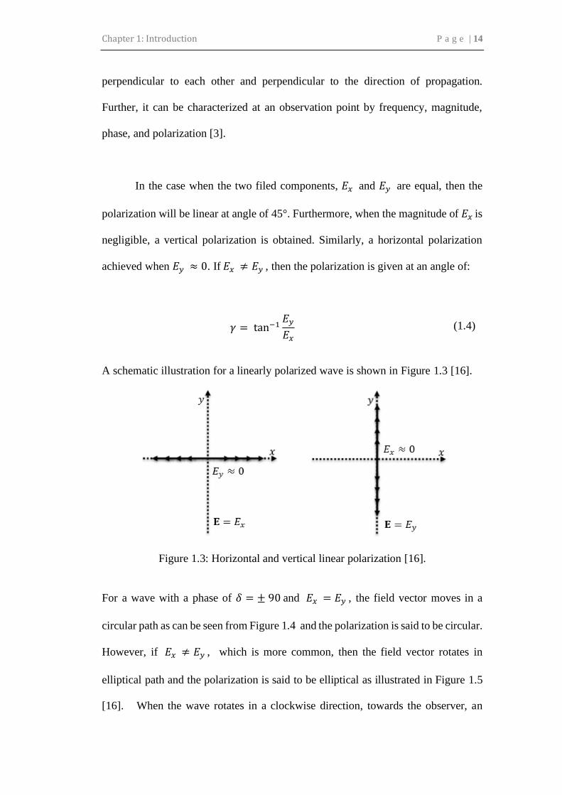
In the case when the two filed components, 𝐸𝑥 and 𝐸𝑦 are equal, then the
polarization will be linear at angle of 45°. Furthermore, when the magnitude of 𝐸𝑥 is
negligible, a vertical polarization is obtained. Similarly, a horizontal polarization
achieved when 𝐸𝑦 ≈ 0. If 𝐸𝑥 ≠ 𝐸𝑦 , then the polarization is given at an angle of:
𝛾 = tan−1𝐸𝑦
𝐸𝑥 (1.4)
A schematic illustration for a linearly polarized wave is shown in Figure 1.3 [16].
Figure 1.3: Horizontal and vertical linear polarization [16].
For a wave with a phase of 𝛿 = ± 90 and 𝐸𝑥 = 𝐸𝑦 , the field vector moves in a
circular path as can be seen from Figure 1.4 and the polarization is said to be circular.
However, if 𝐸𝑥 ≠ 𝐸𝑦 , which is more common, then the field vector rotates in
elliptical path and the polarization is said to be elliptical as illustrated in Figure 1.5
[16]. When the wave rotates in a clockwise direction, towards the observer, an

Chapter 1: Introduction P a g e | 15
LHCP radiation is accomplished. On the other hand, if the wave rotates in an anti-
clockwise direction, a RHCP radiation is obtained.
Figure 1.4: Left-handed and Right-handed circular polarization [16].
Figure1.5: Elliptical polarization [16].
Circular polarization is defined by the Axial Ratio (AR), which is the ratio of the
maximum and minimum semi axes of the ellipse and is given in decibels by [17]:
𝐴𝑅 = 20 log10
𝐸𝑚𝑎𝑥
𝐸𝑚𝑖𝑛 (1.5)

Chapter 1: Introduction P a g e | 16
from which it can be noticed that 1 ≤ 𝐴𝑅 ≤ ∞. A pure circular polarisation can be
achieved when AR = 1 or 0 dB, which is difficult to achieve in practice. Therefore,
a frequency range over which AR ≤ 3 dB is considered and defined as:
𝐴𝑅𝐵𝑊 = 𝑓2 − 𝑓1
𝑓𝑚𝑖𝑛 (1.6)
where, 𝑓2 and 𝑓1 are the boundary frequencies for AR ≤ 3 dB and 𝑓𝑚𝑖𝑛 is the
frequency of minimum value of AR.
CP antennas offer a distinct advantage over their LP counterpart. That is,
there is no need to establish a similar orientation between the transmitter and the
receiver. As a result, the probability of linking a transmitted CP wave is higher since
it can be received in the horizontal, vertical as well as any plane in-between. In
contrast, LP wave is capable of radiating in one plane only, which is particularly
inefficient for mobile and satellite applications. Moreover, a CP wave that is
transmitting in all planes is less susceptible to unwanted reflection and absorption.
Reflecting surfaces may scatter the wave with a different phase, which results in a
weak LP signal.
However, a CP wave can be received regardless of the reflected plane.
Additionally, CP antennas are capable of reducing the Faraday rotation effects,
which means that a linearly polarized wave may be rotated by an unknown amount
depending on the thickness and temperature of the ionosphere, as well as the
frequency and therefore causes a reduction of 3 dB in the signal strength of linearly

Chapter 1: Introduction P a g e | 17
polarized antennas [18], [19]. On the other hand, CP antennas tend to lose their
polarization and become elliptically polarized in the case of non-normal incident. In
addition, CP waves lose their sense if reflected by a PEC, with 180° reflection phase,
which may change a RHCP wave into a LHCP wave or vice versa. Therefore, CP
antennas are not recommended for indoor radio communications [19].
1.1.2.5 Antenna Axial Ratio (AR)
AR of the polarization ellipse is the ratio of its major to minor axes length [14][15].
An AR close to one (0 dB) indicates good CP where, AR greater than one indicates
RHCP and less than one indicates LHCP, and an AR close to infinity indicates good
linear polarization. Calculations for AR are shown in equation (1.7) [20].
For GNSS applications, the AR is usually specified at the antenna boresight
because the AR will increase along with the increase in boresight angle (which
decreases with the increase in elevation angle). Low AR is desirable for most of the
elevation angles. At the upper hemisphere elevation angles (above 10°), the boresight
AR should be less than 3 to 6 dB for a high performance GNSS application. AR
should be between 0 dB to 1 dB for the high-end GNSS application antennas like
choke ring and geodetic quality antennas [21].
𝐴𝑥𝑖𝑎𝑙 𝑅𝑎𝑡𝑖𝑜, 𝐴𝑅 = 𝐸𝑚𝑎𝑗𝑜𝑟
𝐸𝑚𝑖𝑛𝑜𝑟= [
𝐸𝑅𝐻𝐶𝑃 + 𝐸𝐿𝐻𝐶𝑃
𝐸𝑅𝐻𝐶𝑃 − 𝐸𝐿𝐻𝐶𝑃]
(1.7)

Chapter 1: Introduction P a g e | 18
where,
𝐸𝑚𝑎𝑗𝑜𝑟 and 𝐸𝑚𝑖𝑛𝑜𝑟 are the length of the major and minor axes of the polarization
ellipse,
𝐸𝑅𝐻𝐶𝑃 and 𝐸𝐿𝐻𝐶𝑃 are the complex RHCP and LHCP antenna responses (in volts)
𝐸𝑅𝐻𝐶𝑃 = 1
√2(𝐸𝜃 + 𝐸𝜑) (1.8)
𝐸𝐿𝐻𝐶𝑃 = 1
√2(𝐸𝜃 − 𝐸𝜑) (1.9)
𝐸𝜃 and 𝐸𝜑 are the linear field components along 𝜃 and φ directions (in volts) and 𝜃
and φ are spherical coordinates.
1.1.2.6 Antenna Pattern
The upper hemisphere GNSS antenna radiation pattern should have sufficient and
uniform gain and efficiency to effectively receive the GNSS SV signals at the various
azimuth and elevation angles in the upper hemisphere [22]. For most GNSS
applications, the antenna should have a uniform radiation pattern over the upper
hemisphere with a sharp roll off at the lower elevations to reduce the multipath and
lower hemisphere interference [22]. GPS receivers typically use a mask angle of 10°
at the lower elevation angles to minimize multipath and atmospheric effects [23].

Chapter 1: Introduction P a g e | 19
1.1.2.7 Desired to Undesired Ratio
The multipath rejection performance of an antenna can be investigated with the help
of a desired (D) to undesired (U) signal ratio; in general, the multipath due to the
ground reflections can be mitigated by passing the D signals at positive elevation
angles into a reasonable gain GNSS antenna and by attenuating the U signals at the
corresponding negative elevation angles with the help of an antenna radiation
pattern. In this research, D/U is calculated by taking the antenna RHCP gain (in dB)
difference between the positive and negative elevation angles [24].
1.1.2.8 Antenna Phase Reference
The antenna phase response will vary as a function of the azimuth and elevation
angle. The antenna phase response can be measured with respect to an Antenna
Reference Point (ARP) where the measured antenna phase response can then be used
to compensate for these antenna phase variations, with respect to the ARP, depending
upon the performance requirement [25].
1.1.3 Design Challenges: Size Constraints, Feed Network, and Cost
Challenges facing the design of GNSS receive antennas stem from two major
premises: the greatly enlarged. Bandwidth requirement and the constraints by the
platform on which the antenna operates. Feed network and cost are other major
challenges. These are discussed as follows.

Chapter 1: Introduction P a g e | 20
1.1.3.1 Size Constraint
Antenna size constraint and simultaneous broad banding are conflicting
requirements facing fundamental physical limitations, established in a rigorous
analysis six decades ago [26], which relates the fundamental limitation of the gain
bandwidth of an antenna to its electrical size. Also, for a GNSS antenna, its platform
(in a broad sense including the platform’s immediate environment) dictates how, and
how well, the antenna can mitigate problems due to multipath signals from satellite
platform, ionosphere, troposphere, and terrestrial environment, as well as natural and
human-made interferences and noises.
1.1.3.2 Feed Network
The feed network bridges between a coaxial cable and the radiating aperture,
providing excitation to generate RHCP. Since the GNSS antenna needs to detect
extremely low GNSS signals, about 25 dB below noise level on Earth, the use of
LNA close to the antenna is highly desirable. LNA elevates the signal strength so
that it would not be attenuated away before reaching the receiver, usually via a cable
1 to 3 m long, which adds more noise as well.
Additionally, the LNA augments frequency filtering and further enhances
SNR. Because of the high-performance benefit and low cost, use of LNA as part of
GNSS antenna is ubiquitous today. For high performance, a user may select antenna
and LNA separately. With the transition from the narrowband and mostly single
band, GPS to the multiband broadband GNSS, feed network design will be

Chapter 1: Introduction P a g e | 21
fundamentally changed not only by performance considerations but also by
production cost issues. This challenge will be even more serious in the more complex
feed network of anti-interference GNSS arrays with the fixed or adaptive gain
pattern.
1.1.3.3 Cost
The cost of a GNSS antenna is a fundamental design consideration driven by the
market. A testimony is the patch antenna, whose widespread use is not only due to
its low-profile, platform-compatible structure, and medium to small size, but also for
its low cost enabled by its simple feed. However, the patch antenna’s performance
and cost advantages will be challenged by other antennas in the new
multiband/broadband GNSS scenario.
1.1.4 Basic GNSS Antenna Approaches
It is also desirable to know the basic antenna approaches for GNSS antennas. The
answers can be found in several books [17], [19], [27]–[30] covering GNSS
antennas, as well as in general antenna books, outside the GNSS context, under the
category of antennas of CP with a broad symmetrical unidirectional beam and a peak
directivity of 3 – 10 dBi (A higher directivity leads to a narrower beam, and thus a
higher cutoff angle 𝜃𝑐 above the horizon).

Chapter 1: Introduction P a g e | 22
Wang et al. in [6] summarized the basic antenna types applicable to GNSS
and a broad overview of their characteristics in Table 1.3. Patch antennas are the
most common and have a very wide range of variations, e.g., slot-loaded patch
antennas, stacked patch antennas, E-patch antennas, etc. However, the patch antenna
is a resonant antenna, thus inherently narrowband; many elaborate efforts have been
made to add more bands and bandwidth.
The four-element ring arrays consist of four radiating elements fed with a
four-way hybrid or beam-former of 0° - 90° - 180° - 270° to effect RHCP. Each
radiating element can be a slot, a conducting patch of some shape such as a triangle,
a Vivaldi element, an H-slot antenna, or an F or inverted-F antenna, etc. As a
multiband GNSS antenna, it is necessary that the element radiators have some
inherent broadband or multiband potential.
The spiral antenna and the quadrifilar helix antenna are also common GNSS
antennas. Planar spiral antennas have several variations, mostly for changing their
bidirectional radiation to unidirectional. The traveling-wave (TW) antenna is one
technique that overcomes this problem by employing the spiral or other broadband
planar radiators and having a closely spaced conducting ground plane [31], [32].

Chapter 1: Introduction P a g e | 23
Table 1.3: Basic Antenna Types Used in GNSS and Their General Characteristics [6]

Chapter 1: Introduction P a g e | 24
1.2 RESEARCH MOTIVATION AND OBJECTIVES
Modern GNSS technology is facing more challenges and new fields for researchers
to explore. One hot topic is the multi-system GNSS device. Many research groups
have demonstrated that a multi-system GNSS receiver (e.g., GPS and Galileo) will
usually provide more observations than a single-system receiver which provides
higher positioning precision. Accordingly, such a multi-antenna system requires
compact design which brings a new challenge for the antenna engineers.
Meanwhile, compact design always makes the commercial GNSS antenna
more competitive compared with larger size antenna with similar performance.
Smaller is always better. The motivation for the antenna designers is to miniaturise
the size of the antenna and meanwhile keep its standard performance.
The objective of this research is to design, simulate and investigate the
performance of a circularly polarized antenna prototype, which is expected to operate
at GNSS frequency bands from 1.16 GHz to 1.6 GHz to cover the GPS L1-L5 bands,
GLONASS G1, G2 and G3 as well as the Galileo E5a, E5b, E6, and E1bands with
good multipath mitigation. A printed dipole design is chosen for this prototype
because of the following merits: ease of fabrication and mounting, multipath
performance, relatively low profile, easy integration with active components.

Chapter 1: Introduction P a g e | 25
1.3 CONTRIBUTIONS AND ORGANIZATION OF THIS
THESIS
This thesis consists of seven chapters that mainly focus on design, optimization, and
measurement of novel broadband antennas for GNSS applications. The structure of
the thesis and the outcome and achievements of each chapter is discussed briefly in
this section to give a better view of the work. The chapters are organized as follows:
• Chapter 1 introduces the background of this work, including the motivation
and objectives of the research in this thesis.
• Chapter 2 is an overview and fundamentals of GNSS system and a brief
introduction about interference, jamming attack and jamming effect on GNSS.
The history of the system and communication are discussed.
• Chapter 3 gives an overview of the development on GNSS receiver antenna
design using the different type of antennas and its design parameters with a
detailed literature review of the state-of-art for these applications. Then, it
discusses the antenna diversity systems, and the existing crossed-dipole
antenna designs for GNSS applications in detail.
• Chapter 4 introduces a new broadband with broad beamwidth antenna to cover
the GPS L1-L5 bands, GLONASS G1, G2 and G3 as well as the Galileo E5a,
E5b, E6 and E1bands (1.08 GHz – 1.69 GHz). This broadband antenna
demonstrates a significant improvement on bandwidth and radiation pattern by
using the parasitic elements and loaded monopoles that are excited by coupling
with the elliptical crossed dipole in the center of the antenna.
• Chapter 5 presents a new way of designing a dual-band CP antenna by
integrating a CP radiator with a finite AMC surface. The antenna demonstrates

Chapter 1: Introduction P a g e | 26
a low-profile broadband characteristic and excellent CP radiation for GNSS
frequency bands.
• Chapter 6 introduces a new optimized antenna that more compact from the
previous antenna discussed in Chapter 4 and 5. This chapter also presents a
new antenna array configuration combining a 4-elements antenna array and a
5-elements antenna array to provide wide coverage. The anti-jamming
performance of the antenna with respect to differently polarized jammers as
well as its positioning capability are also presented.
• Finally, Chapter 7 provides a summary of the major contributions of this thesis.
In addition, some future work recommendations for this research topic are
suggested.

Chapter 2: GNSS System Overview P a g e | 27
CHAPTER 2:
GNSS SYSTEM OVERVIEW
2.1 INTRODUCTION
The role of the Global Positioning Satellite System (GNSS) has become
indispensable in our lives. Because of its significance, research is very active in this
sector and obtaining higher reliability, and higher accuracy is essential to sustain the
integrity of the position, velocity, and time (PVT) solutions. Initially, a military
satellite system that was later provided partially to the public, GNSS system has seen
explosive growth in the number of users. There are also many industry sectors that
rely on it such as precise timing, precise positioning used in geodesy and structural
engineering, aviation, land and maritime navigation, etc. [3].
This chapter starts with a general introduction of the GNSS system’s sectors
followed by the GNSS observables, the generic structure of the receiver and finally

Chapter 2: GNSS System Overview P a g e | 28
a summary of the GNSS errors which will pave the way towards the main objectives
of this research. Interference and jamming are then overviewed; where their types,
causes, sources, effects, and mitigation techniques are described.
2.1.1 GPS Fundamentals
Operated by the United States, GPS is the best-known satellite-based radio
navigation and positioning system among the GNSS, which provides accurate and
instantaneous Position, Velocity and Timing (PVT) services for an unlimited number
of civilian and military users in all weather conditions. A GPS receiver needs at least
four visible satellites to calculate the three-dimensional position and time solution.
Any GNSS including GPS system is mainly made up of three major segments (see
Figure 2.1):
• Space Segment (SS) or Satellite
• Segment Control Segment (CS) or Operational Control Segment (OC)
• User Segment (US)
Figure 2.1: GPS segments.

Chapter 2: GNSS System Overview P a g e | 29
2.1.1.1 Space Segment (SS)
GPS constellation as shown in Figure 2.2 consists of 24 operational satellites in six
orbital planes with four satellites in each plane. It has been recently upgraded to 27
by the US air force [33]. The number of satellites can increase up to 30. The
ascending nodes of the orbital planes are separated by 60 degrees, and the orbital
planes are inclined 55°. The orbit of each GPS satellite is nearly circular with a semi-
major axis of 26578 km and a period of about twelve hours. The satellites
continuously orient themselves to ensure that their solar panels stay pointed towards
the Sun, and their antennas point toward the Earth. Each satellite carries four atomic
clocks, is the size of a car and weighs about 1000 kg [34].
Figure 2.2: Expandable 24-slot satellite constellation[33].

Chapter 2: GNSS System Overview P a g e | 30
2.1.1.2 Control Segment (CS)
The control segment of GPS is made up of a network of tracking stations positioned
across the Earth as shown in Figure 2.3 with a master control station (MCS) located
at Colorado Springs, Colorado, USA. This MCS is staffed around the clock. There
are 16 monitoring stations located throughout the globe. Six of them are operated
from Air Force bases and ten from the National Geospatial-Intelligence Agency
(NGA) [33]. They are located around the Earth, and their positions are known very
precisely. These stations are equipped with very sophisticated GPS receivers and a
cesium oscillator for tracking all the satellites in view. The MCS remotely operates
these ground control stations.
Figure 2.3: Locations of the different sections of the control segment around the
world [33].
Among the tasks of the control segment are: (a) monitoring and maintaining
satellite orbits and health by maneuvering and relocation, (b) maintaining GPS time,
Chapter 2: GNSS System Overview P a g e | 31
(c) predicting satellite ephemerides and clock parameters and (d) updating satellite
navigation messages periodically [3].
2.1.1.3 User Segment (US)
The user segment consists of users (individuals, commercial or military) with
different radio receivers that receive signals from GPS satellites and estimate their
position, velocity, and time. Users of GPS can be classified into civil and military.
The user segment is experiencing exponential growth since inauguration due to
decreasing prices of the receiver and the increasing application of GPS in daily life.
When a GPS receiver is activated, it will acquire the GPS satellite signals [35]. The
signal is processed, and the receiver position is determined by the intersection of the
spheres created by the satellite pseudoranges. A minimum of four satellites with good
geometry is required. Three satellites are required for the position fix, while the
fourth is required to account for the receiver clock offset. An in depth look at the
user segment can be found in [36] and [1].
2.1.2 GLONASS Fundamentals
GLONASS is a Russian version of a GNSS that provides the three-dimensional PVT
services across the globe in all weather conditions, similar to GPS made up of a,
satellite Space Segment, monitoring Control Segment, and User Segment. The Space
Segment has eight, equally spaced satellites (a total of 24) in three orbital planes.
Each satellite takes 11 hours, 15 minutes and 44 sec to complete an orbit with 64.8°
inclination to each other [37]. The GLONASS transmission frequency is determined

Chapter 2: GNSS System Overview P a g e | 32
by its channel number, K and its frequency bands are calculated using the following
expression.
𝑓𝐿1 (𝐾) = 𝑓𝐿1 + 𝐾∆𝑓𝐿1 (2.1)
𝑓𝐿2 (𝐾) = 𝑓𝐿2 + 𝐾∆𝑓𝐿2 (2.2)
where,
𝑓𝐿1 = 1602 𝑀𝐻𝑧 𝑎𝑛𝑑 ∆𝑓𝐿1 = 562.5 𝑘𝐻𝑧 𝑓𝑜𝑟 𝐿1 𝑠𝑢𝑏 𝑏𝑎𝑛𝑑 𝑎𝑛𝑑
𝑓𝐿2 = 1246 𝑀𝐻𝑧 𝑎𝑛𝑑 ∆𝑓𝐿2 = 437.5𝑘𝐻𝑧 𝑓𝑜𝑟 𝐿2 𝑠𝑢𝑏 𝑏𝑎𝑛𝑑
The Control Segment consists of a satellite tracking and command stations network
located across Russia to monitor the satellites and provide the corrections to the
orbital parameters and navigation data as needed [37]. The User Segment is equipped
with receiver equipment to receive and process the GLONASS signals transmitted
by the satellites to determine the user PVT solution. GLONASS historically has used
FDMA in similar frequency bands as GPS (i.e., L1, L2, L5), and is now developing
a CDMA-based GLONASS GNSS.
2.1.3 Galileo Fundamentals
Galileo is the European GNSS, which is planned to provide highly accurate global
positioning services to various users. Once deployed completely, the Galileo Space
segment will consist of 27 operational satellites and three spare operational satellites
(total 30) in three circular MEO orbit planes inclined at 56° and 29,601.297 km semi
Chapter 2: GNSS System Overview P a g e | 33
major axis. The Control Segment and User Segment are similar to GPS and
GLONASS as discussed earlier.
2.1.4 Signal Characteristics
These satellite systems are fundamentally similar, and one can typically develop
technology that generally applies to all of them. The research presented in this work,
which focuses on the receiver antenna and its associated signal processing that
applicable to any GNSS system so long as the antenna and antenna electronics are
designed for the required frequencies. In this work, we will frequently use the term
“GNSS antenna” to refer to an antenna designed for any one or multiple satellite
navigation systems. Each GNSS satellite uses an array of transmit antennas to
broadcast RHCP Electromagnetic (EM) energy with a radiation pattern that aims to
evenly cover the entire visible portion of the earth. As mentioned above, this signal
is quite weak, and it is modulated with unencrypted Pseudo Random Noise (PRN)
code and navigation data. In this section, these three properties of the GNSS signal:
its RHCP nature, its low signal strength, and its use of PRN codes will be discussed.
2.1.4.1 RHCP Electromagnetic (EM) Energy
EM energy propagates through free space, such as the space between the GPS
satellites and our antenna, at the speed of light. EM energy also propagates along
conductive structures, such as ground-planes and the coaxial cables that deliver the
energy from the antenna to the receiver, at near the speed of light. The waves that

Chapter 2: GNSS System Overview P a g e | 34
travel from the satellites to our antenna take the form of transverse electromagnetic
plane waves.
Figure 2.4: An RHCP wave where the red spiral traces the RHCP energy, and the
blue and green sinusoidal waves trace the contributions from the x-axis and y-axis
field components [38].
In the case of GNSS, these electromagnetic plane waves are RHCP. An
RHCP wave can be decomposed into two orthogonal electric field components,
which called as an x-axis field and a y-axis field for some arbitrary coordinate system
in the plane parallel to the plane wave. These two field components are orthogonal
not only in space but also in time, with the x-axis field lagging the y-axis field by
90°, as can be seen in Figure 2.4. The red spiral traces the RHCP energy while the
blue and green sinusoidal waves trace the contributions from the x-axis and y-axis
field components.

Chapter 2: GNSS System Overview P a g e | 35
2.2 INTERFERENCE AND JAMMING
As mentioned earlier, interference and jamming signals prevent RF front-end from
functioning correctly. It has been reported in [2] that no matter what tracking and
acquisition have been implemented in the digital part of the receiver, they will be
rendered useless. The latter condition is true if the GPS signals were totally corrupted
by the nonlinear behavior of the front-end. Spectral characteristics such as the carrier
frequency and bandwidth, 𝑓𝑖𝑛𝑡 and 𝐵𝑖𝑛𝑡 respectively, can lead to a broad
classification of interferences. A higher-level classification would include in-band
and out of band signals.
Table 2.1: Classification of Interferences Based on Spectral Characteristics
Class Spectral Characteristics
Out-of-band interference
𝑓𝑖𝑛𝑡 > 𝑓𝐼𝐹 + 𝐵𝐼𝐹
2
or
𝑓𝑖𝑛𝑡 < 𝑓𝐼𝐹 − 𝐵𝐼𝐹
2
In-band interference (𝑓𝐼𝐹 − 𝐵𝐼𝐹
2 < 𝑓𝑖𝑛𝑡 < 𝑓𝐼𝐹 +
𝐵𝐼𝐹
2 )
Wideband interference 𝐵𝑖𝑛𝑡 ≈ 𝐵𝐼𝐹
Narrowband interference 𝐵𝑖𝑛𝑡 ≪ 𝐵𝐼𝐹
The former would encompass any signal whose carrier frequency is close but
outside the GPS band while the latter would encompass signals found inside the GPS
band. A more specific classification for the in-band interferences would differentiate

Chapter 2: GNSS System Overview P a g e | 36
between the bandwidths of different interference sources and categorize them into
narrowband and wideband interferences.
The different classifications are demonstrated in Table 2.1 where 𝐵𝐼𝐹 and 𝑓𝐼𝐹
correspond to the GPS signal’s bandwidth and center frequency after the IF stage
[39]. Most interference signals are generated by licensed emitters that do not transmit
in the L1 band; nonetheless, harmonics of these signals find their way into the GPS
L1 band.
A summary of the different types of interference signals based on their
modulation types as well as their potential sources is shown in Table 2.2. Some of
the most common interference and jamming sources are demonstrated in Figure 2.5.
Figure 2.5: Common interference and jamming source.

Chapter 2: GNSS System Overview P a g e | 37
Table 2.2: Types of RF Interference and Their Probable Sources
Class Type Potential Sources
Narrowband Continuous Wave
(CW)
Intentional CW jammers or near-band
unmodulated transmitter’s carriers
Narrowband Swept CW Intentional swept CW jammers or
frequency modulation (FM) stations
transmitters’ harmonics
Narrowband Phase/ frequency
modulation
Intentional chirp jammers or harmonics
from an amplitude modulation (AM) radio
station, citizens band (CB) radio, or
amateur radio transmitter
Wideband Pulse Any type of burst transmitters such as
radar or ultra-wideband (UWB)
Wideband Wideband -
matched spectrum
Intentional matched-spectrum jammers,
spoofers, or nearby pseudolites
Wideband Wideband -
phase/frequency
modulation
Television transmitters’ harmonics or near
band microwave link transmitters
overcoming the front-end filter of a GPS
receiver
Wideband Wideband -
bandlimited
Gaussian
Intentional matched bandwidth noise
jammers
Chapter 2: GNSS System Overview P a g e | 38
2.2.1 Jamming Attack on GNSS
GNSS anti-jamming was always considered a priority of the military sector,
unfortunately, due to primarily, the growing demand of personal privacy devices
(PPDs), [40]–[43] jamming is being viewed as a threat to the public; especially with
the increasing dependence on the GNSS system. Jamming attacks have a sole
objective of preventing the receiver from providing the desired solution. Although
jamming is illegal and therefore criminalized, it has been reported that offenders have
been using jammers to prevent stolen vehicles from being tracked or simply to
remain undetected. Equally, PPDs are becoming cheaper and easier to acquire
leading to the increased threat of GNSS outages for the everyday consumer [44][45].
Therefore, the struggle against jamming has been moved from the battlefield to the
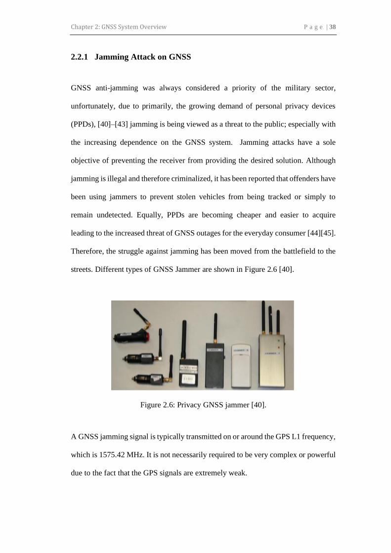
streets. Different types of GNSS Jammer are shown in Figure 2.6 [40].
Figure 2.6: Privacy GNSS jammer [40].
A GNSS jamming signal is typically transmitted on or around the GPS L1 frequency,
which is 1575.42 MHz. It is not necessarily required to be very complex or powerful
due to the fact that the GPS signals are extremely weak.

Chapter 2: GNSS System Overview P a g e | 39
The jamming signal can effortlessly overwhelm the GPS receiver’s front-end
and prevent the actual signal from being processed. Unfortunately, this occurs
because the spreading gain (approximately 30 dB) is not yet applied to the signal. At
that time, even after the spreading gain is applied, the jamming signal is also
amplified therefore preventing further processing of GPS signals. The gain of the
amplifier adjusts itself to the jamming signal, which is more powerful.
2.2.2 Jamming Effect on GNSS
Several studies [40], [41] have explored the effects of jamming and especially PPDs
on Global Navigation Satellite Systems (GNSS) performance. Jamming deteriorates
the positioning solution accuracy, leads to the total loss of lock on the satellite signals
and therefore impairs the positioning availability. It has been reported that the typical
front end is saturated in case of broadband additive white Gaussian noise (AWGN)
signals, high power narrowband and pulsed signals. Contrarily, the front-end was not
saturated when low power narrowband, spoofing and meaconing signals were
applied. Several authors have studied the effects of jamming on acquisition and
tracking [46]–[49]. Acquisition success is documented in [49]; where it has been
identified that CW has the most damaging effect compared to swept CW and
broadband noise which come in second place such that 10 and 15 dB Jamming to
Signal Ratios (JSR) is required to prevent acquisition respectively.
Chapter 2: GNSS System Overview P a g e | 40
2.3 ANTI-JAMMING TECHNIQUE
Successive detection is followed by mitigation if the receivers are equipped for it. A
multitude of techniques has been proposed for anti-jamming and interference
suppression. They can be classified mainly into single antenna-based techniques,
which perform jamming mitigation based on receiver processing, whether in pre-
correlation or post-correlation, and antenna array-based techniques, which benefit
from the presence of the array to spatially mitigate the jamming signals by
electronically controlling the radiation pattern of the array. Since all the mitigation
techniques used by single antenna systems are present in the receiver, then it is
appropriate to imply that they are all applicable in multi-antenna systems.
2.3.1 Single Antenna Receiver-based Solutions
Mitigation solutions in the front-end of the receiver are usually accomplished either
using spectral or temporal excision. Mitigation of certain types of interference such
as pulsed interference can be accomplished using a technique called pulse blanking.
It is an appropriate technique aimed at mitigating pulsed interference. Interference
excision is implemented in the time domain on the samples obtained from the ADC
that are above a certain threshold. Alternatively, frequency excision is implemented
in the front-end; it is based on determining the frequencies occupied by the
interference signal.
Typically, a jammer is used to jam the signals of specific GNSSs and not all
systems at the same time. Nevertheless, such jammers can be acquired at an

Chapter 2: GNSS System Overview P a g e | 41
expensive cost. A solution for this problem is to switch to another GNSS when
service denial is sensed, such as GPS, GLONASS, GALILEO and BEIDOU (which
has limited coverage). Switching from one GNSS to another requires more advanced
hardware such as multiple frequency antennas and multi-constellation capable
receivers.
2.3.2 Antenna Array Based Solutions
An antenna array is a group of antennas for which the outputs are combined to create
an overall radiation pattern that is different from that of each antenna element
individually [50]. These antennas are arranged in space depending on the array
geometry. They are processed such that the radiation pattern of the array increases
the gain towards a selected direction while rejecting signals emitted from other
directions [51].
Thus, the interference signal(s) are rejected in space, rather than in the
frequency or time domain. Interference mitigation is significantly enhanced by using
an adaptive antenna array (also known as a smart antenna) through the capabilities
of spatial filtering techniques. These techniques frequently attain high anti-jamming
(AJ) margins. They are effective against both narrow and especially broadband
interference signals that single antenna systems cannot combat [52].
Hence, adaptive arrays improve SNR in the presence of jamming which
enables signal tracking in environments that would otherwise lack code and carrier

Chapter 2: GNSS System Overview P a g e | 42
phase observables. The most common techniques applied in adaptive spatial filtering
are null steering and beamforming.
2.3.2.1 Null Steering
Null steering, also known as side lobe canceller (SLC), is based on the fact that the
GPS signal power is lower than the noise floor. Null Steering considers any signal
with a power level higher than that of the satellite to be an interference signal.
Accordingly, the antenna’s beam is steered away from that source and a null is
directed towards it. The objective is to decrease the output power subject to the
constraint that one antenna element is always on while trying to maintain unit gain
in all other directions. The rest of the channels have their output phase and amplitude
adjusted in order to block jammers.
2.3.2.2 Beamforming
Beamforming, on the other hand, enhances signal reception by directing beams
towards desired signals. The desired antenna outputs are weighted using different
sets of complex beamforming coefficients. In the case of GNSS, multiple beams are
required; one for every satellite. Maximizing the power of the beam achieved by
beamforming will also utilize the available degrees of freedom to shape the spatial
null and minimize GNSS signal cancellation.
Therefore, the probability that GPS signals will be preserved increases. It is a
known disadvantage of null steering that there will be a probable reduction in the

Chapter 2: GNSS System Overview P a g e | 43
received GNSS signal’s energy level and especially if the signal’s Direction of
Arrival (DoA) is close to the interferer’s DoA [53].
2.4 SUMMARY
In this chapter, GNSS antenna technologies and overview have been reviewed. It has
been clearly shown that the research of GNSS antenna is of great significance to the
modern industry and it will still be an important research topic for the coming
decades. The studies of antenna for GNSS applications have been highlighted and
discussed in detail. The information presented in this chapter is useful to gain a better
understanding on the state of art in antenna designs and meanwhile identify the
research challenges and problems for us to overcome in this work.

Chapter 3: GNSS Receiver Antenna Design: Overview and State of The Art P a g e | 44
CHAPTER 3:
GNSS RECEIVER ANTENNA DESIGN: OVERVIEW
AND STATE OF THE ART
3.1 INTRODUCTION
Global navigation satellite systems (GNSSs), including global positioning system
(GPS), GLObal NAvigation Satellite System (GLONASS), Galileo, and Compass,
will be fully deployed and operational in a few years [6]. An antenna for a GNSS
receiver requires broadband characteristics for such as impedance matching and 3-
dB axial ratio (AR) bandwidths, right-hand circularly polarized (RHCP) radiation, a
wide CP radiation beamwidth (> 100°) facing the sky, and a high front-to-back ratio.
The use of a variety of single and dual-band CP antennas in the GNSS
frequency bands has been reported: e.g., crossed dipole [54]–[58], monopole [59]–
[62], slotted [63]–[68], patch [69]–[74] and dielectric resonator [75]–[79] antennas.
However, most of these antennas have insufficient 3-dB AR beamwidth to meet the

Chapter 3: GNSS Receiver Antenna Design: Overview and State of The Art P a g e | 45
requirements of GNSS applications, owing to the lack of techniques to broaden the
CP radiation beamwidth.
3.2 GNSS ANTENNA: OVERVIEW
A CP antenna for multi-frequency operation can be achieved by using multi-layer
patches. By using a multi-layer structure, it is easier to achieve a multi-frequency CP
operation. The dimensions of each patch mainly determine the resonant frequencies.
The geometry of the proposed antenna is shown in Figure 3.1.
Figure 3.1: Geometry of the stacked patch CP antenna (a) side view (b) upper patch
(c) middle patch and (d) lower patch [70].

Chapter 3: GNSS Receiver Antenna Design: Overview and State of The Art P a g e | 46
A single probe feed of 50Ω input impedance is connected to the upper patch through
via holes in the middle and lower patches while the middle and lower patches are
excited through electromagnetic coupling. The via has contributed a capacitive
coupling to negate the inductance effect due to the inner conductor of the probe. The
use of slit on the edge of the lower patch introduces the dual orthogonal mode
necessary for CP radiation pattern. Both the middle and upper patches are perturbed
by corner truncation which produces near degenerated resonant mode resulting in
CP.
(a)
(b)
Figure 3.2: (a) Measured and simulated reflection coefficients of the antenna and
(b) Simulated axial ratio of the proposed antenna [70].

Chapter 3: GNSS Receiver Antenna Design: Overview and State of The Art P a g e | 47
Falade et al. [70] have proposed a design on stacked patches with a single
feed for GPS frequency bands. The lower, middle, and upper patches are designed
to resonate at L5, L2, and L1 frequency bands respectively. The patches are etched
on three different substrates. The lower substrate has a thickness of ℎ3 = 1.524 mm
and relative permittivity 휀𝑟 = 3.38, the middle and upper substrates are similar with
a thickness of ℎ2 = ℎ1 =1.6 and permittivity of 휀𝑟 = 4.4.
The measured value of 10 dB impedance bandwidth for GPS L1, L2, and L5
frequency bands are 22 MHz (2.0%), 18 MHz (1.5%), and 30 MHz (2.0%),
respectively are shown in Figure 3.2. The simulated axial ratio at broadside direction
illustrates that the minimum axial ratio coincides with the resonant frequencies in the
three bands. The 3-dB axial ratio bandwidth is 40 MHz (3.40%) in L5 frequency
band, 10 MHz (0.81%) in L2 frequency band, and 13 MHz (0.83%) in L1 frequency
band.
CP can also be generated by using a dielectric resonator antenna [75]–[77],
[80]–[82]. A hybrid antenna comprising a dielectric resonator antenna (DRA) and
four feed slots as shown in Figure 3.3 has been investigated and analyzed to enhance
the AR bandwidth in order to cover the current GNSS frequency bands in one
antenna [77]. The cylindrical DRA has a radius of 31.75 mm, a height of 22 mm and
a permittivity of 10. It has been designed to resonate around 1.575 GHz. CP is
generated by a 90° phase feed network. The slots have to be arranged and their
dimensions optimized to ensure proper coupling to the dielectric resonator and to
have good impedance matching. A substrate made of FR4 was chosen to
accommodate the feed circuit of the DRA, and the slots were etched in the ground

Chapter 3: GNSS Receiver Antenna Design: Overview and State of The Art P a g e | 48
plane. The ground plane dimensions are 160 × 160 mm2, and the slot length is 36
mm, and its width is 8.8 mm. The coordinates of the slots are 4 mm along the x-
direction and 19.4 mm in the y-direction. The feed line is 12.9 mm long and 11 mm
away from the slot center. The prototype of the DRA and its performance are shown
in Figures 3.3 and 3.4. However, the disadvantage of the hybrid DRA over other
GNSS antennas is its bulky in size.
Figure 3.3: The diagram of the hybrid DRA[77].

Chapter 3: GNSS Receiver Antenna Design: Overview and State of The Art P a g e | 49
(a)
(b)
(c)
Figure 3.4: Hybrid DRA performance measured (a) S11 (b) maximum radiation gain
and (c) axial ratio [77].

Chapter 3: GNSS Receiver Antenna Design: Overview and State of The Art P a g e | 50
Two novel broadband single-feed printed compact wideband circularly
polarized antennas as described in [59], consisting of L-shaped monopole and tilted
cross on the ground plane with and without a slanted branch. By introducing a
protruding cross at the ground, wideband CP is generated. The antenna has a very
compact structure with a dimension of 88 × 88 mm2 on the substrate. The antenna
uses FR-4 substrate 1.6 mm thick with a permittivity of 4.4.
(a) (b)
Figure 3.5: Fabricated prototype of (a) antenna 1 (b) antenna 2 [59].
The geometry of the proposed broadband planar antenna with broadband CP
is shown in Figure 3.5. All the metallic components of the antenna are printed on the
same side of the substrate. The antenna consists of a square ground with a cross-
shaped branch at its corner. The simulated and measured reflection coefficient and
boresight AR of two antennas are compared in Figure 3.6 (a) and (b).
In Figure 3.6 (a), antenna 1 exhibits simulated (excluding the cable model) and
measured -10 dB impedance bandwidths of 54.71%, from 1.130 to 1.981 GHz, and
55.10%, from 1.160 to 2.042 GHz, respectively. Besides, antenna 2 exhibits
simulated (excluding the cable model) and measured -10 dB impedance bandwidths
of 68.70%, from 1.096 to 2.243 GHz, and 70.44%, from 1.122 to 2.344 GHz,

Chapter 3: GNSS Receiver Antenna Design: Overview and State of The Art P a g e | 51
respectively. The results reveal that the slant branch is useful to improve the
impedance matching. Figure 3.6 (b) shows that antenna 1 has measured 3-dB AR
bandwidths at dual bands 1.356 -1.637 GHz (18.78%) and 1.794 - 2.487 GHz
(32.38%). Also, antenna 2 has measured 3dB AR bandwidths at dual bands 1.270 -
1.600 GHz (23.00%) and 1.750 - 2.450 GHz (33.33%). The measured results agree
well with the simulated results with the inclusion of the cable model. If the feed cable
was excluded, 1.130 - 1.981 GHz (54.71%) and 1.096 - 2.243 GHz (68.70%) CP
bands for two antennas are predicted in simulation, which is broad enough to cover
GNSS spectra.
(a)
(b)
Figure 3.6: Simulated and measured (a) reflection coefficient and (b) axial ratio
[59].

Chapter 3: GNSS Receiver Antenna Design: Overview and State of The Art P a g e | 52
3.3 GNSS CROSSED-DIPOLE ANTENNA
S. X. Ta et al. [56] have proposed a multi-band, RHCP, crossed, multi-branch,
barbed dipole antenna with a broad impedance-matching bandwidth, and a high
front-to-back ratio in the GPS L1 - L5 bands. The multi-branch barbed dipole with a
meander line in each branch is used to achieve not only multiple resonances but also
a significant reduction in the radiator size. A vacant quarter printed ring is used as a
90° phase delay line to generate the CP radiation.
Along with the development of wireless communications, many applications
require antennas that radiate a unidirectional pattern with a significant front-to-back
ratio to ensure high security and efficiency in the propagation channels. Accordingly,
the crossed dipole is generally equipped with a reflector to generate a desired
unidirectional pattern with CP or dual polarization [83].
The antenna is composed of two printed dipoles, a coaxial line, and a
reflector. The reflector is an inverted pyramidal cavity with a rectangular bottom
measuring 120 × 120 mm2, a top aperture measuring 160 × 160 mm2, and a height
of 40 mm as shown in Figure 3.7.

Chapter 3: GNSS Receiver Antenna Design: Overview and State of The Art P a g e | 53
(a)
(b)
(c)
Figure 3.7: Geometry of the proposed antenna (a) radiator (b) vacant-quarter
printed ring and dipole arm (c) side view with the inverted pyramidal cavity [56].
The crossed dipole was designed on both sides of a 60 × 60 mm2 Rogers
RO4003 substrate with permittivity of 3.38 and thickness of 0.508 mm. The outer
conductor of the coaxial line is connected to the arms on the bottom side of the
substrate. The inner conductor of the coaxial line extends through the substrate and

Chapter 3: GNSS Receiver Antenna Design: Overview and State of The Art P a g e | 54
connects to the arms on the top side. The crossed dipoles are equipped with a cavity-
backed reflector to provide a unidirectional radiation pattern with a wide AR
beamwidth and a high front-to-back ratio in both bands.
(a)
(b)
Figure 3.8: Simulated and measured (a) reflection coefficients (b) axial ratios of the
multi-band antenna [56].

Chapter 3: GNSS Receiver Antenna Design: Overview and State of The Art P a g e | 55
The proposed antenna has bandwidths of 1.131–1.312 GHz (181 MHz),
1.369–1.421 GHz (52 MHz), and 1.543–1.610 GHz (67 MHz) for impedance
matching with |S11| < -10 dB and 1.165–1.190 GHz (25 MHz), 1.195–1.240 GHz (45
MHz), 1.370–1.395 GHz (25 MHz), and 1.565–1.585 GHz (20 MHz) for an AR of
< 3dB as shown in Figure 3.8.
On the other hand, [84] reported a novel composite cavity with unequal-
length crossed fins is designed and integrated with the antenna to enhance the front-
to-back ratio (FBR) of the antenna. It is well known that the surface wave
propagating along the ground plane reradiates at the ground plane edge and thus
increases the side-lobes as well as the back lobe of the antenna. Therefore,
suppressing the propagation of surface waves can reduce the back lobe of the
antenna.
Figure 3.9: Geometry of the proposed antenna with a composite cavity [84].
The antenna is etched on a 0.817 mm thick Rogers RO4003C substrate with a relative
permittivity of 3.55 and a loss tangent of 0.0027. Furthermore, the patches are
employed to tune the impedance matching of the proposed antenna by introducing
proper capacitance. Similar to the conventional crossed dipole CP antenna, the

Chapter 3: GNSS Receiver Antenna Design: Overview and State of The Art P a g e | 56
proposed antenna radiates in bidirectional that makes RHCP toward the broadside
and LHCP backward. The proposed composite cavity placed underneath the antenna
shows better back lobe reduction ability by minimizing diffracted waves.
(a)
(b)
Figure 3.10: (a) Prototype of ultra-wideband composite cavity backed CP antenna
and VSWR and (b) simulated and measured ARs of the antenna with and without a
cavity [84].
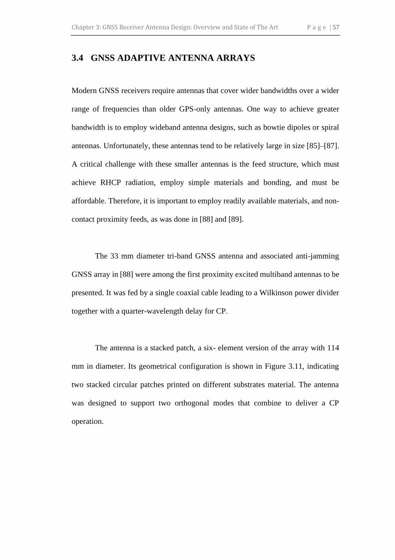
Chapter 3: GNSS Receiver Antenna Design: Overview and State of The Art P a g e | 57
3.4 GNSS ADAPTIVE ANTENNA ARRAYS
Modern GNSS receivers require antennas that cover wider bandwidths over a wider
range of frequencies than older GPS-only antennas. One way to achieve greater
bandwidth is to employ wideband antenna designs, such as bowtie dipoles or spiral
antennas. Unfortunately, these antennas tend to be relatively large in size [85]–[87].
A critical challenge with these smaller antennas is the feed structure, which must
achieve RHCP radiation, employ simple materials and bonding, and must be
affordable. Therefore, it is important to employ readily available materials, and non-
contact proximity feeds, as was done in [88] and [89].
The 33 mm diameter tri-band GNSS antenna and associated anti-jamming
GNSS array in [88] were among the first proximity excited multiband antennas to be
presented. It was fed by a single coaxial cable leading to a Wilkinson power divider
together with a quarter-wavelength delay for CP.
The antenna is a stacked patch, a six- element version of the array with 114
mm in diameter. Its geometrical configuration is shown in Figure 3.11, indicating
two stacked circular patches printed on different substrates material. The antenna
was designed to support two orthogonal modes that combine to deliver a CP
operation.

Chapter 3: GNSS Receiver Antenna Design: Overview and State of The Art P a g e | 58
(a)
(b)
(c)
Figure 3.11: (a) Prototype using high-contrast substrates and (b) associated
Wilkinson divider for feeding using a single coax feed at Port 1 and (c) gain of the
patch [88].

Chapter 3: GNSS Receiver Antenna Design: Overview and State of The Art P a g e | 59
The geometrical parameters for the feed in Figure 3.11 (b) that were found to
achieve good gain at all frequencies are: D = 33 mm, 𝑑1 = 26 mm, 𝑑2= 22 mm, ℎ1 =
6mm, and ℎ2 = 8 mm. Figure 3.11 also shows the boresight gain curves, which show
2.5 dBi to 5 dBi at the lower (L5/ E5a, E5b, and L2) and higher (L1) bands.
Referring to Figure 3.11, this GNSS antenna covers all said bands and has the
following optimized parameters. The simulated and measured gain performance is
shown in Figure 3.11 (c). Its gain in the bands of interest is always greater than 0 dB
and even reaches more than 4 dBi at some bands. Specifically, the lower mode of the
stacked patches covers the L5/ E5a, E5b, and L2 bands with RHCP gain above 3-dB,
whereas the high mode covers the L1 band with a gain of 5 dBi.
For the array formation, the antenna in Figure 3.11 was used to form a six-
element circular array shown in Figure 3.12. Key to this performance is coupling
reduction between adjacent antenna elements within the array.
For smaller array sizes, it is important to reduce the antenna element size even
further than shown above. A 25 mm GNSS antenna element was first presented by
Zhou et al. [90]. Instead of using higher-contrast dielectric substrates that would
reduce bandwidth, slots are introduced on the printed surface of the GPS antenna. A
similar concept was introduced in [91] and [92] adopted four spiral slots to design a
proximity-fed dual-band stacked patch.
Chapter 3: GNSS Receiver Antenna Design: Overview and State of The Art P a g e | 60
(a)
(b)
Figure 3.12: (a) GNSS antenna array design and (b) fabricated prototype [88].
Kasemodel et al. [85] and Svendsen et al. [93] presented a spiral array antenna
capable of continuous operation from 1.1 to 1.6 GHz. The array is shown in Figure
3.13. The array is designed to be placed on a ground plane, making it suitable for
mounting on small vehicles. In [85], the dielectric layer is formed from a polymer,
allowing precise control of its dielectric constant while also reducing weight and
increasing mechanical durability as compared to more rigid and brittle dielectric
materials.

Chapter 3: GNSS Receiver Antenna Design: Overview and State of The Art P a g e | 61
Figure 3.13: Four-element and six-element spiral array [85], [93].

Chapter 3: GNSS Receiver Antenna Design: Overview and State of The Art P a g e | 62
The array elements are connected in the center with resistors, and ferrite
beads are used to terminate the spiral arms. These techniques improve return loss
and axial ratio while maintaining good gain and upper hemispherical coverage. In
the absence of interference, the array is designed to operate in a reference mode
where all elements are excited with equal weight and progressive phase. This
produces a rotationally symmetric boresight pattern with RHCP polarization. The
densely packed array produces significant mutual coupling between elements.
However, the array has been designed with each element effectively exciting the
entire aperture. The small size of the array and the wideband nature of the spiral
results in desirable phase and delay characteristics.
Meanwhile, in [93] altered the square spiral array in [85] and presented a
dual-band array for handheld GPS receivers. Handheld applications are more
challenging since the antenna array must be extremely lightweight, be very robust,
occupy a small volume, be inherently portable, and be easy to fabricate. The array
presented in consists of a tightly packed 2 × 2 array of square spiral elements that
form a small, 4 × 4 inch2 (102 × 102 mm2) aperture that can flip out from a handheld
receiver. Again, the array operates in a reference mode with no interference. The
resulting RCHP polarized pattern is broad with good peak realized gain. The authors
show simulations of the antenna performance with space-time adaptive processing
(STAP). They demonstrate their ability to operate in scenarios with several
narrowband and wideband interference sources.

Chapter 3: GNSS Receiver Antenna Design: Overview and State of The Art P a g e | 63
(a)
(b)
Figure 3.14: (a) Antenna array geometry formed by five identical patch antennas
and (b) radiation pattern at φ = 0° and φ = 90° [94].
A recent study by [94] has proposed a new method to extract the optimal
complex weights for suppression of the jamming signals in a GPS antenna array in

Chapter 3: GNSS Receiver Antenna Design: Overview and State of The Art P a g e | 64
the presence of mutual coupling. The proposed antenna array geometry is shown in
Figure 3.14. All patch antennas are printed on a square RO4003 substrate with a
length of L = 20 cm, 30 mm thickness and relative permittivity of 휀𝑟 = 3.55.
The full wave simulation patterns of the standalone GPS antenna element and
the reference active element patterns in the array (fifth elements) is shown in Figs.
3.14(a) and (b). It shows the normalized antenna radiation patterns comparison at φ
= 0, 90˚ planes where the antenna gain is 5.24 and 3.94 dB for the stand alone and
reference antennas, respectively. The null steering method was performed by using
the exact active element patterns of the array antenna. These patterns include the
mutual coupling effect and the nearby antenna scattered such as holder which
increase the antenna performance to deal with the jammer sources which was not
considered in the literature based on the author knowledge.
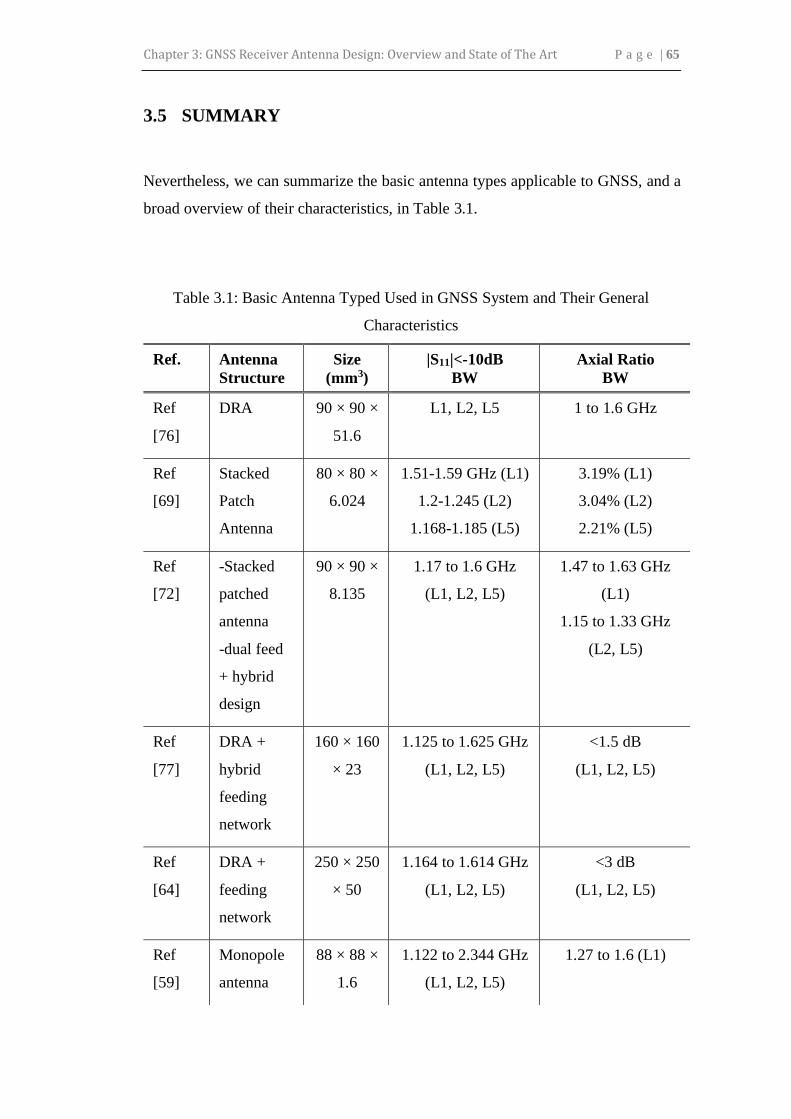
Chapter 3: GNSS Receiver Antenna Design: Overview and State of The Art P a g e | 65
3.5 SUMMARY
Nevertheless, we can summarize the basic antenna types applicable to GNSS, and a
broad overview of their characteristics, in Table 3.1.
Table 3.1: Basic Antenna Typed Used in GNSS System and Their General
Characteristics
Ref. Antenna
Structure
Size
(mm3)
|S11|<-10dB
BW
Axial Ratio
BW
Ref
[76]
DRA 90 × 90 ×
51.6
L1, L2, L5 1 to 1.6 GHz
Ref
[69]
Stacked
Patch
Antenna
80 × 80 ×
6.024
1.51-1.59 GHz (L1)
1.2-1.245 (L2)
1.168-1.185 (L5)
3.19% (L1)
3.04% (L2)
2.21% (L5)
Ref
[72]
-Stacked
patched
antenna
-dual feed
+ hybrid
design
90 × 90 ×
8.135
1.17 to 1.6 GHz
(L1, L2, L5)
1.47 to 1.63 GHz
(L1)
1.15 to 1.33 GHz
(L2, L5)
Ref
[77]
DRA +
hybrid
feeding
network
160 × 160
× 23
1.125 to 1.625 GHz
(L1, L2, L5)
<1.5 dB
(L1, L2, L5)
Ref
[64]
DRA +
feeding
network
250 × 250
× 50
1.164 to 1.614 GHz
(L1, L2, L5)
<3 dB
(L1, L2, L5)
Ref
[59]
Monopole
antenna
88 × 88 ×
1.6
1.122 to 2.344 GHz
(L1, L2, L5)
1.27 to 1.6 (L1)

Chapter 3: GNSS Receiver Antenna Design: Overview and State of The Art P a g e | 66
In this chapter, some significant achievements in GNSS antenna technologies
have been reviewed. It has been clearly shown that the research of GNSS antenna is
of great significance to the modern industry and it will still be an important research
topic for the coming decades. The studies of antenna for GNSS applications have
been highlighted and discussed in detail. It was found that most existing antennas in
the literature have not been focused on broadband antennas due to the difficulty and
complexities in the design. The information presented in this chapter is useful to gain
a better understanding on the state of art in antenna designs and meanwhile identify
the research challenges and problems for us to overcome in this work.
Ref
[57]
Crossed-
dipole
antenna
120 × 120
× 30.55
1.274 to 2.360
(L1, L2)
1.39 to1.82 GHz
(L1, L2)
Ref
[55]
Crossed-
dipole
antenna
120 × 120
× 40
1.555 to 1.665 GHz
(L1)
1.220 to 1.385 GHz
(L2)
1.565 to 1.595 GHz
(L1)
1.260 to 1.300 GHz
(L2)
Ref
[95]
Crossed-
dipole
antenna
120 × 120
× 62.5
1.05 to 1.79
(L1, L2, L5)
1.12 to 1.64 GHz
(L1, L2, L5)

Chapter 4: Performance Analysis of CP Antenna for GNSS Applications P a g e | 67
CHAPTER 4:
A CROSSED-DIPOLE ANTENNA WITH PARASITIC
ELEMENTS
4.1 INTRODUCTION
With the deployment of a few noteworthy Global Navigation Satellite Systems
(GNSSs) for example GPS, GLONASS, COMPASS and many more frequency
bands will be accessible for positioning applications. GNSS applications have
multiplied internationally, not only in the military field but also in business and
consumer markets.
Global positioning systems typically transmit in CP due to its features of non-
sensitive to Faraday rotation introduced by the ionosphere and its potential of
reducing polarization mismatch and multipath interferences. Different designs of
single and dual-band CP antennas in the GNSS frequency bands have been reported:

Chapter 4: Performance Analysis of CP Antenna for GNSS Applications P a g e | 68
e.g., crossed dipole [58], monopole [59], slotted [64], [65], stacked patch [69], [70]
and dielectric resonator [75]–[77] antennas. Nevertheless, almost all these antennas
have inadequate 3-dB AR bandwidth to meet the requirements of GNSS applications,
due to the lack of techniques to broaden the CP radiation bandwidth. Recently,
single-feed CP antennas with a compact radiator have been designed for GNSS
applications [55], [56]. However, their operational bandwidth does not completely
cover the GNSS spectra.
This chapter presents a broadband and broad beamwidth circularly polarized
antenna to cover the GPS L1-L5 bands, GLONASS G1, G2 and G3 as well as the
Galileo E5a, E5b, E6 and E1bands (1.08 GHz – 1.69 GHz). A printed vacant-quarter
ring is used as a 90-degree phase delay line between the dipole pair to produce the
CP radiation. The detailed dimensions are presented, and good results are obtained.
The CST Microwave Studio is employed for the numerical simulation.
4.2 AN ANTENNA WITH PARASITIC ELEMENTS
4.2.1 Antenna Design Configurations
Figure 4.1 and Table 4.1 show the geometry and the dimension of the proposed
broadband CP antenna, respectively. The antenna comprises two printed cross
dipoles and a coaxial line. The dipoles are printed on both sides of a Rogers RO3210
substrate with a relative permittivity of 10.2 and thickness of 1.28 mm.

Chapter 4: Performance Analysis of CP Antenna for GNSS Applications P a g e | 69
Figure 4.1: Geometry of the proposed antenna: (a) top view and (b) side view.
Table 4.1: Dimension of The Proposed Antenna
Parameter Value (mm) Parameter Value (mm)
Lg 90.0 L 66.0
R1 4.7 R2 5.5
W1 20.0 W2 8.0
W3 8.5 H1 15.5
The proposed antenna is designed to meet the needs of multiple GNSS. The
critical part is the feeding structure which is relatively new, and the dimensions
should be optimized. The elliptical cross-dipole antenna is produced on both sides of
the PCB board. The antenna was fed with a 50 Ω coaxial line. The outer conductor
of the coaxial line was connected to the dipole arms on the bottom side of the

Chapter 4: Performance Analysis of CP Antenna for GNSS Applications P a g e | 70
substrate while the inner conductor of the coaxial line was extended through the
substrate and connected to the dipole arms on the top side.
The pair of dipoles is linked by a vacant quarter printed ring to generate 90°
phase delay line and produce the RHCP radiation field at the front side of the antenna
and the LHCP radiation field at the back side. The reason of choosing the cross-
dipole in this design are the impedance bandwidth of the cross-dipole is much
broader than a conventional microstrip patch antenna, and it is much easier o
generate the CP radiation and obtain a broader CP bandwidth by using the feeding
mechanism as mentioned above.
Furthermore, the antenna is composed of four parasitic element and four
metallic cylinder that are excited by coupling with the elliptical crossed dipole in the
center. Figure 4.2 shows the theory of how to broaden the beamwidth. The ordinary
microstrip antenna radiates mainly towards the elevation angle of 90°. Meanwhile,
the crossed dipoles radiate mainly towards the elevation angle of 0°. Therefore, when
the ordinary microstrip antenna is combined with the loaded monopoles, the two-
elevation angle of highest gain of the two radiation patterns could be merged into
one, and their radiation fields are added together, forming a broad radiation pattern
in both the 𝑋𝑜𝑍 and 𝑌𝑜𝑍 planes. Based on this theory and our numerical simulations,
the vertical half power beamwidth (HPBW) of the microstrip antenna could be
widened.

Chapter 4: Performance Analysis of CP Antenna for GNSS Applications P a g e | 71
(a) (b) (c)
Figure 4.2: Vertical radiation patterns for the antennas. (a) elliptical cross-dipole
(b) parasitic element and loaded monopole and (c) crossed dipole surrounded by
parasitic elements and monopoles.
By adjusting the size of the parasitic elements and the edge of the dipoles, the
coupling strength can be optimized. The antenna was optimized via CST Simulation
Software. For the initial design of the proposed antenna, it was first to design in free
space to provide resonance in the GPS L1 and L2 bands.
4.2.2 Antenna Performances
The simulated 𝑆11, axial ratio and gain of the antenna with different values of the
ground plane length 𝐿𝑔 are depicted in Figures 4.3 to 4.4, respectively. The
bandwidth of the antenna for 𝑆11 < -10 dB is improved by reducing the size of the
ground plane. The impedance bandwidth of the antenna covers from 1.08 to 1.69
GHz when the size of ground plane is 90 mm × 90 mm which is completely cover
the entire GPS bands (L1: 1.575 GHz, L2: 1.227 GHz, L3: 1.381 GHz, L4: 1.379
GHz and L5: 1.175 GHz) and Galileo (E1; 1.575 GHz, E5: 1.191 GHz and E6: 1.279
GHz).

Chapter 4: Performance Analysis of CP Antenna for GNSS Applications P a g e | 72
Meanwhile, the CP bandwidth (AR < 3-dB) shows a decrease at the lower
frequency when the size of the ground plane is reduced, but at the upper frequency
bands, the axial ratio is reduced. It covers from 1.55 to 1.63 GHz which involves the
L1 and E1 frequency bands and from 1.12 to 1.26 GHz for L2, L5, and E5.
Figure 4.3: The simulated S11 with different values of 𝐿𝑔 of the proposed antenna.
Figure 4.4: The simulated axial ratio with different values of 𝐿𝑔 of the proposed
antenna.
S11
(dB
)
Frequency (GHz)
Axia
l R
atio
(d
B)
Frequency (GHz)
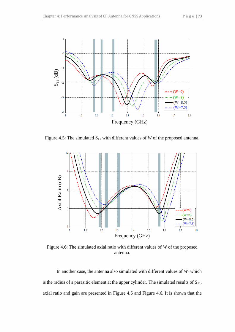
Chapter 4: Performance Analysis of CP Antenna for GNSS Applications P a g e | 73
Figure 4.5: The simulated S11 with different values of W of the proposed antenna.
Figure 4.6: The simulated axial ratio with different values of W of the proposed
antenna.
In another case, the antenna also simulated with different values of W3 which
is the radius of a parasitic element at the upper cylinder. The simulated results of S11,
axial ratio and gain are presented in Figure 4.5 and Figure 4.6. It is shown that the
Axia
l R
ati
o (
dB
)
Frequency (GHz)
S11
(dB
)
Frequency (GHz)

Chapter 4: Performance Analysis of CP Antenna for GNSS Applications P a g e | 74
impedance bandwidth of the antenna did not change much, but the resonant
frequency seems to be shifted to the higher frequency bands when the radius of the
parasitic element is too small.
However, as shown in Figure 4.6, the CP bandwidth (AR < 3-dB) is highly
sensitive to the variation of the parasitic element size. The axial ratio decreased when
the size of the parasitic element is enlarged at the lower frequency. Meanwhile, at
the upper frequency bands, the axial ratio decreased when the size of the element
reduced. The optimal value of W is 8.5 mm to cover the desired bandwidth. Thus, as
shown in Figure 4.6, when W = 8.5, the CP bandwidth for AR < 3-dB is from 1.13
to 1.22 GHz for L2, L5, and E5 bands and from 1.53 to 1.59 GHz for L1 and E1
bands.
Figure 4.7: The simulated radiation pattern with and without the parasitic elements
of the proposed antenna at (a) GNSS L2 (b) GNSS L1.

Chapter 4: Performance Analysis of CP Antenna for GNSS Applications P a g e | 75
The simulated radiation patterns are demonstrated in Figure 4.7, indicating
that hemispherical shape radiation patterns with good symmetry is obtained. It can
be seen that the radiation pattern is greatly enhanced by the introduction of the
parasitic elements for both operating bands.
Figure 4.8 presents the RHCP radiation patterns in two orthogonal planes.
For both the 𝑋𝑜𝑍 and 𝑌𝑜𝑍 planes, the HPBW is more than 170°. The operation at
other frequencies is given in Table 4.2. At each frequency, the antenna shows a wide
angular coverage for both HPBW and 3-dB axial ratio beamwidth.
Figure 4.8: RHCP radiation patterns in 𝑋𝑜𝑍 and 𝑌𝑜𝑍 planes at 1.575 GHz.
Table 4.2: 3 dB Beamwidth of The Proposed Antenna
Frequency band HPBW (deg)
𝑿𝒐𝒁 / 𝒀𝒐𝒁
3-dB axial ratio
beamwidth (deg)
𝑿𝒐𝒁 / 𝒀𝒐𝒁
GNSS: L1 172 / 170 157 / 140
GNSS: L2 120 /120 140 / 120
GNSS: L5 180/174 134 / 156

Chapter 4: Performance Analysis of CP Antenna for GNSS Applications P a g e | 76
The final design was fabricated and measured. The comparison of the
simulated and measured reflection coefficients of the fabricated antenna is shown in
Figure 4.9 (a) and (b). The antenna was measured in an anechoic chamber using a
vector analyzer. The simulated and measured reflection coefficients of the antenna
are depicted in Figure 4.10.
It can be seen that the results agreed reasonably well within the bandwidth.
The |S11|< –10 dB measured bandwidths of the lower and upper bands were merged,
and the result ranged from 1.060 to 1.671 GHz. The simulated bandwidths were
1.077–1.683 GHz. Figure 4.11 shows the simulated and measured axial ratio of the
proposed antenna. It can be seen that a very good agreement was obtained between
simulation and measurement. The CP bandwidth AR ˂ 3-dB is from 1.093 to 1.257
GHz (164 MHz) and 1.542 to 1.666 GHz (124 MHz) as expected.
(a) (b)
Figure 4.9: Photograph of fabricated antenna (a) front view and (b) perspective
view.

Chapter 4: Performance Analysis of CP Antenna for GNSS Applications P a g e | 77
1.0 1.1 1.2 1.3 1.4 1.5 1.6 1.7 1.8 1.9 2.0
-20
-15
-10
-5
0
|S1
1| (d
B)
Frequency (GHz)
simulated
measured
Figure 4.10: Measured and simulated results of the proposed antenna: |S11|.
1.0 1.1 1.2 1.3 1.4 1.5 1.6 1.7 1.8
0
3
6
9
Axi
al r
atio
(dB
)
Frequency (GHz)
simulated
measured
Figure 4.11: Measured and simulated results of the proposed antenna: AR.

Chapter 4: Performance Analysis of CP Antenna for GNSS Applications P a g e | 78
4.3 SUMMARY
A new broadband cross-dipole antenna has been proposed and designed for the
GNSS applications. The impedance bandwidth is very broad to cover the entire GPS,
Galileo, and GLONASS bands. The structure of the antenna is compact and unique.
The dimension of the antenna is 90 mm × 90 mm × 15.5 mm which is small and
compact. The proposed antenna has bandwidth of 1.06 to 1.671 GHz (611 MHz) for
impedance matching |S11| < -10 dB and 1.093 to 1.257 GHz (164 MHz) and 1.542 to
1.666 GHz (124 MHz) for an AR < 3-dB. All the results have demonstrated that the
antenna is an excellent candidate for the GNSS application.
Table 4.3: Comparison with Existing GNSS Antenna Designs
Ref. Size (mm3) |S11| <-10 dB BW
(GHz)
Axial Ratio
BW (GHz)
Antenna Type
Ref [16] 160 × 160 × 23 1.125 to 1.625 (L1,
L2, L5, E6)
<1.5dB (L1,
L2, L5)
DRA + hybrid
feeding
network
Ref [5] 88 × 88 × 1.6 1.122 to 2.344
(L1, L2, L5, E6)
1.27 to 1.6 (L1,
E6)
Monopole
antenna
Ref [3] 120 × 120 ×
30.55
1.274-2.360
(L1, L5)
1.39-1.82 (L1) Crossed-dipole
antenna
Proposed
Antenna
90 × 90 × 15.5 1.06 to 1.671
(L1, L2, L5, E6)
1.093 to 1.257
(L5, L2)
1.542 to 1.666
(E6)
Crossed-
dipole antenna

Chapter 4: Performance Analysis of CP Antenna for GNSS Applications P a g e | 79
In order to evaluate the achievements of the proposed antenna with respect to
available designs, the proposed antenna is compared with recently published designs
as tabulated in Table 4.3.

Chapter 5: Performance Analysis of CP Antenna Backed by AMC Ground Plane P a g e | 80
CHAPTER 5:
A CIRCULARLY POLARIZED ANTENNA BACKED
BY AN AMC GROUND PLANE
5.1 INTRODUCTION
Artificial Magnetic Conductor (AMC) is a type of implemented metamaterial in
several antenna and microwave design applications. By utilizing the unique
characteristics of metamaterials which do not exist naturally, the performance of
various microwave devices can be enhanced. This chapter elaborates on the technical
perspective and recent works on AMC for antenna applications. The technical
perspective discusses the theoretical aspects, simulation design procedures, and the
measurement setup used to characterize the AMC unit cell. Subsequently, various
recent works of antenna design that involve the incorporation of AMC are discussed
thoroughly. Each of the recent works is highlighted with specific performance
enhancements that can be achieved with the introduction of AMC.

Chapter 5: Performance Analysis of CP Antenna Backed by AMC Ground Plane P a g e | 81
5.2 ARTIFICIAL MAGNETIC CONDUCTOR (AMC)
AMC is a metamaterial which mimics the characteristics of a perfect magnetic
conductor (PMC). A useful PMC characteristic that mimicked by AMC is the ability
to provide zero-degree reflection phases at its resonant frequency[96].
Electromagnetic band gap (EBG) technology has become a significant breakthrough
in the radio frequency (RF) and microwave applications due to their unique band gap
characteristics at certain frequency ranges.
Since 1999, the EBG structures have been investigated for improving
performances of numerous RF and microwave devices utilizing the surface wave
suppression and the artificial magnetic conductor (AMC) properties of these special
type metamaterial. Issues such as compactness, wide bandwidth with low attenuation
level, tunability, and suitability with planar circuitry all play an important role in the
design of EBG structures.
EBG structure can be defined as fabricated periodic elements that may hinder,
allow, or confine electromagnetic waves propagation within a specified span of
frequencies [97]. These structures are formed by arranging dielectric material and
metallic conductors periodically. When plane waves are incident upon an EBG
structure, the reflection coefficient phase varies with frequency. At a frequency, the
incident wave encounters a reflection phase of zero degrees. At this frequency, the
EBG functions as an AMC. This structure when integrated onto a microstrip antenna
below the radiating patch functions either as a reflector or as an artificial ground
plane [98].

Chapter 5: Performance Analysis of CP Antenna Backed by AMC Ground Plane P a g e | 82
The main problem of an antenna equipped with a metallic reflector is often
addressed by including a quarter-wavelength space between the radiating elements
and the reflector to obtain optimal antenna characteristics. These can be
circumvented by using an AMC surface instead of a metallic reflector. The AMC,
which consists of a lattice of metal plates on a grounded dielectric substrate
with/without grounding vias, can mimic a perfect magnetic conductor (PMC) over a
certain frequency band.
By combining the crossed dipole radiators and the finite AMC surfaces, low-
profile multiband CP antennas that are nearly completely matched to a single 50 Ω
source and have high radiation efficiencies have been implemented. More
interestingly, surface waves propagating on the finite AMC are excited to generate
extra operating bands for the radiating system. It was shown that the extra bands
could be favorably used to enhance the bandwidth of the antenna.
5.2.1 AMC Properties
AMC-based antennas have been intensely developed for enhancing their
performance, including bandwidth and unidirectional radiation pattern with a
miniaturized profile. The AMC surface, also known as a high-impedance surface
(HIS) [99], an EBGs [97], or a reactive impedance surface [100], can mimic a PMC
within a certain frequency range. Therefore, the AMC surface allows for the
placement of the antenna in proximity with good impedance matching and highly
efficient radiation. In many applications, an antenna works at two different
frequencies simultaneously; consequently, the AMC structure requires dual-band

Chapter 5: Performance Analysis of CP Antenna Backed by AMC Ground Plane P a g e | 83
operation that can match the antenna’s working frequencies. Many LP antennas on
AMC surface [101]–[105] have been presented for dual-band operation, but there are
still a limited number of studies on CP antennas loaded with the dual-band AMC
structures. Recently, a dual-band LP dipole was designed on a dual-band
polarization-dependent EBG surface to realize a dual-band CP antenna [106].
However, its AR bandwidth is insufficient for some applications.
AMCs are used in low-profile microstrip antennas to generally improve their
gain and bandwidth [107]–[110] and directivity [111]. Usually AMC cells are
fabricated as periodic structures. However, in [112], a multi periodic AMC structure
is used to improve gain and also to widen the impedance bandwidth of a planar
antenna. In [113], a periodic AMC structure is designed by using genetic algorithm
is found to improve the bandwidth of a wideband planar antenna. Sidelobe
suppression is also possible with AMC structures as investigated in [114].
In addition, AMC can also be implemented in a resonance cavity antenna as
a ground plane to achieve profile reduction by almost one-half, while maintaining
high gain performance [115], [116]. Radar cross-section reduction can also be
achieved by combining two AMCs which have overlapping bandwidths [117]. These
promising improvements on the characteristics of low-profile planar antennas have
triggered various investigations on the possible geometries which form the AMC
structure.
AMC is also known as High Impedance Surface (HIS) because at its resonant
frequency, it exhibits high surface impedance [118]. The surface impedance consists

Chapter 5: Performance Analysis of CP Antenna Backed by AMC Ground Plane P a g e | 84
of real and imaginary parts. AMC can be constructed with and without vias
connection [118]–[121]. However, for incidence wave normal to the AMC, the vias
are not required as there are no currents excited to it [122]. Via is a shorting pin from
the metallic patch of AMC unit cells to the ground as shown in Figure 5.1 (a). As
shown in the figure, the AMC is consisting of several periodically arranged metallic
unit cells of uniform dimensions with individual vias. The equivalent inductance-
capacitance presented in the AMC/HIS structure and the circuit model shown in
Figure 5.1 (b) and Figure 5.1 (c), respectively.
(a)
(b) (c)
Figure 5.1: (a) An array of AMC unit cells with each vias connected to the
ground plane, (b)the equivalent inductance capacitance circuit, and
(c)circuit model [102].
Conventional antenna tends to use Perfect Electric Conductor (PEC) (or in
practical, conductive layer like copper) as a conventional background plane [123].

Chapter 5: Performance Analysis of CP Antenna Backed by AMC Ground Plane P a g e | 85
The PEC layer functions as the reflector of the antenna. However, the drawback of
the PEC layer is the produced reflected wave that is 180° out of phase with respect
to the source wave, J as shown Figure 5.2 (a). The source wave is a wave (wave 1)
that initially flows along the radiating part of the antenna. The out of phase reflected
wave (wave 2) induces destructive interference with the source wave. This
interference cancels out or greatly attenuates the source wave from the antenna,
hence reducing its radiation efficiency.
(a) (b) (c)
Figure 5.2: Antenna separated (a) closely and (b) further from the ground plane.
(c)Antenna incorporated with AMC is in very close proximity with the ground
layer [98].
Subsequently, the gain of the antenna decreases. In this case, the antenna
might not properly match due to the strong field cancellation. The undesired effect
of the PEC layer can be minimized by having the PEC layer at a minimum distance
of λ/4 from the radiating antenna as in Figure 5.2 (b). The corresponding distance
considered the 𝜋 phase shift of the reflected wave (from the PEC) that will
constructively interfere with the source wave (from the antenna). Additionally, the
impedance matching at the resonant frequency is also improved. Unfortunately, the

Chapter 5: Performance Analysis of CP Antenna Backed by AMC Ground Plane P a g e | 86
drawback of the introduction of such distance increases the overall antenna
dimensions.
Thus, the antenna structure is no longer low-profile, a characteristic most
desirable in antenna designs especially in space limited conditions such as in
microwave circuitry of portable devices. In contrast, PMC (or AMC in practical)
generates reflected waves that are similar in the direction of the original current with
the reflection coefficient of magnitude |Г| that equals to +1. As illustrated in Figure
5.2 (c), the reflected wave by AMC is in-phase with the source wave.
The additional reflected waves constructively interfere with the source wave.
The combining effect from both reflected wave and source wave improves the
radiation efficiency and gain of the antenna. Thus, a low-profile antenna can be
realized without adding an unnecessary distance of λ/4 between the AMC ground
plane and the antenna (as in the case of PEC ground layer).
5.3 CP CROSSED-DIPOLE ANTENNA WITH AMC SURFACE
ON FR-4 SUBSTRATE
5.3.1 Antenna Design Configurations
A new way of designing a dual-band CP antenna by integrating a CP radiator with a
finite AMC surface. The broadband operation was obtained in Figure 5.3. It consists
of a compact crossed dipole above a 5 × 5 AMC surface. The antenna was optimized

Chapter 5: Performance Analysis of CP Antenna Backed by AMC Ground Plane P a g e | 87
for GNSS frequency bands with low-profile broadband characteristics and excellent
CP radiation.
(a)
(b)
Figure 5.3: Geometry of the proposed antenna: (a) top and (b) cross-sectional view
of the proposed antenna.
The proposed antenna is designed to meet the needs of multiple GNSS. The
critical part is the feeding structure which is relatively new, and the dimensions
should be optimized. The elliptical cross-dipole antenna is produced on both sides of
the PCB board. The antenna was fed with a 50 Ω coaxial line. The outer conductor

Chapter 5: Performance Analysis of CP Antenna Backed by AMC Ground Plane P a g e | 88
of the coaxial line was connected to the dipole arms on the bottom side of the
substrate while the inner conductor of the coaxial line was extended through the
substrate and connected to the dipole arms on the top side.
Figure 5.3 shows the geometry of the dual-band, crossed, asymmetric dipole
antenna on the dual-band AMC surface. The crossed dipoles were suspended at a
height from the top of the reflector. The primary radiator element, which is similar
to the one presented in Chapter 4, was designed on both sides of PCB.
Figure 5.3 (b) shows the geometry of the unit cell of the AMC structure. A 5
× 5 metal patch array forming an AMC surface was backed as a reflector of the
proposed antenna. The unit cell was printed on a 100 mm × 100 mm FR-4 substrate
with a relative permittivity of 4.4, a loss tangent of 0.0023, and a thickness of 10
mm. There was no via. Four slits were symmetrically inserted into the square patch
of the AMC unit cell. A sample of the fabricated antenna is shown in Figure 5.4. The
AMC structure was optimized via adjusting the slit shape to have the resonances
frequency.

Chapter 5: Performance Analysis of CP Antenna Backed by AMC Ground Plane P a g e | 89
(a)
(b)
(c)
Figure 5.4: Photograph of the fabricated antenna (a),(b) front view and (c) back
view.

Chapter 5: Performance Analysis of CP Antenna Backed by AMC Ground Plane P a g e | 90
5.3.2 Antenna Performances
The crossed asymmetric dipoles were first optimized in free space for GNSS
frequency bands with good CP radiation and then incorporated with PEC and AMC
reflectors to render a unidirectional radiation pattern. To achieve a unidirectional
radiation pattern, good impedance matching, and good low-profile CP radiation at
both operating bands, a crossed asymmetric dipole antenna was incorporated with
the AMC surface. Interactions between the radiator and the reflector, such as the air
gap and finite size of the AMC surface, were meticulously considered for the
optimization.
1.0 1.2 1.4 1.6 1.8 2.0
-40
-35
-30
-25
-20
-15
-10
-5
0
|S11| (
dB
)
Frequency (GHz)
simulated_
measured_
Figure 5.5: Measured and simulated results of the proposed antenna: |S11|.
The overall size of the final design was 100 mm × 100 mm × 14 mm including
the substrate thickness of the radiator. Since a 10 mm thick FR-4 sheet was

Chapter 5: Performance Analysis of CP Antenna Backed by AMC Ground Plane P a g e | 91
unavailable, the AMC was fabricated by stacking several thin sheets and binding
them together by using four plastic screws (not included in the simulations) to
achieve the desired thickness.
The crossed asymmetric dipole on the dual-band AMC surface was fabricated
and measured. A comparison of the simulated and measured |S11| and AR values is
given in Figure 5.5 and Figure 5.6. The measured impedance bandwidths of 10 dB
were 1.196 to 2.176 GHz, values that agree closely with the simulated bandwidths
of 1.607 to 1.845 GHz.
The measured AR < 3-dB bandwidths were 1.148 to 1.761 GHz, while the
simulated AR <3-dB bandwidths were 1.1803 to 1.795 GHz.
1.0 1.1 1.2 1.3 1.4 1.5 1.6 1.7 1.8
0
3
6
9
simulated
measured
Frequency (GHz)
Axi
al R
atio
(dB
)
Figure 5.6: Measured and simulated results of the proposed antenna: AR.

Chapter 5: Performance Analysis of CP Antenna Backed by AMC Ground Plane P a g e | 92
(a)
(b)
Figure 5.7: Measured and simulated results of the radiation pattern at (a) L1 and (b)
radiation pattern at L2.
Figure 5.7 (a) and (b) shows the radiation patterns of the antenna at 1.575 GHz
(L1) and 1.227 GHz (L2), respectively. The measurements agreed well with the CST
simulation results and showed RHCP radiation, a wide CP radiation beamwidth, and
asymmetric pattern in both the xz and yz planes. At 1.575 GHz, the measurements
resulted in a gain of 5.9 dBic, a front-to-back ratio of 24 dB, and a 3-dB AR
beamwidth of 200° and 199° in the xz and yz planes, respectively. At 1.227 GHz, the
measurements resulted in a gain of 6 dBic, a front-to-back ratio of 24 dB, and a 3-
dB AR beamwidth of 168° and 150° in the xz and yz planes, respectively.
Additionally, the measured radiation efficiencies were about 90% and 87%, and the
simulated values were 95% and 89%, at 1.227 GHz and 1.575 GHz, respectively.

Chapter 5: Performance Analysis of CP Antenna Backed by AMC Ground Plane P a g e | 93
5.4 CP CROSSED-DIPOLE ANTENNA WITH AMC SURFACE
ON ROGERS RT6006 SUBSTRATE
5.4.1 Antenna Design Configurations
Figure 5.8 shows the geometry of the proposed antenna which comprised of two
printed dipoles as a primary radiator which is similar to the one presented in Chapter
4, was designed on both sides of PCB, a coaxial line, and an AMC surface. The
printed dipoles were suspended at height H above the AMC surface. The AMC was
composed of 5 × 5 square metal patch structures that were periodically printed on
the conductor-backed substrate.
Figure 5.8 (b) shows the geometry of the unit cell of the AMC structure. A 5
× 5 metal patch array forming an AMC surface was backed as a reflector of the
proposed antenna. The unit cell was printed on a 100 × 100 mm2 Rogers RT 6006
substrate with a relative permittivity of 4.4, a loss tangent of 0.0023, and a thickness
of 12.7 mm as shown in appendices section. There was no via. Four slits were
symmetrically inserted into the square patch of the AMC unit cell. A sample of the
fabricated antenna is shown in Figure 5.9.

Chapter 5: Performance Analysis of CP Antenna Backed by AMC Ground Plane P a g e | 94
(a)
(b)
(c)
Figure 5.8: Geometry of the proposed antenna: (a) top and (b) cross-sectional view
of the proposed antenna (c) perspective view.

Chapter 5: Performance Analysis of CP Antenna Backed by AMC Ground Plane P a g e | 95
Figure 5.9: Photographs of the fabricated antenna.

Chapter 5: Performance Analysis of CP Antenna Backed by AMC Ground Plane P a g e | 96
The AMC structure was optimized via adjusting the slit shape to have the
resonances frequency. The AMC substrate was made of an RT6006 material with a
relative permittivity of 10.2 and a loss tangent of 0.0023. The characteristic
impedance of the coaxial line was 50 Ω, and the line passed through the center of the
AMC reflector to feed the radiator. The antenna was optimized via CST Simulation
Software.
5.4.2 Antenna Performances
This design using a 5 × 5 cell AMC configuration with H = 12.7 mm was fabricated
and measured. The printed dipoles were fabricated on both side of FR-4, and AMC
reflector was fabricated on RT6006. Because a 12.7 mm thick RT6006 sheet was
unavailable, the AMC was fabricated by stacking two sheets and binding them
together by tape to achieve the desired thickness. The antenna was measured in an
anechoic chamber using a network analyzer.
The comparison of the simulated and measured reflection coefficients of the
antenna is shown in Figure 5.10. The |S11|< –10 dB measured bandwidths of the
lower and upper bands were merged, and the result ranged from 1.153 to 2.36 GHz.
The simulated bandwidths were 1.154 to 1.929 GHz. The slight difference between
the measurement and the simulation could be attributed to the effects of the binding
process.

Chapter 5: Performance Analysis of CP Antenna Backed by AMC Ground Plane P a g e | 97
1.0 1.2 1.4 1.6 1.8 2.0
-40
-35
-30
-25
-20
-15
-10
-5
0
|S11| (
dB
)
Frequency (GHz)
simulated_
measured_
Figure 5.10: Measured and simulated results of the proposed antenna: |S11|.
1.0 1.1 1.2 1.3 1.4 1.5 1.6 1.7 1.8
0
3
6
9
simulated
measured
Frequency (GHz)
Axi
al R
atio
(dB
)
Figure 5.11: Measured and simulated results of the proposed antenna: AR.

Chapter 5: Performance Analysis of CP Antenna Backed by AMC Ground Plane P a g e | 98
Figure 5.11 shows the measured and simulated AR bandwidth values of the
antennas, which also yielded a good agreement between the two. The measured 3-
dB AR bandwidths were 1.170 – 1.970 GHz. The simulated 3-dB AR bandwidths
were 1.199 – 1.9 GHz. Figure 5.12 (a-d) shows the radiation patterns of the crossed
dipole on the AMC surface at L5 (1.176 GHz), L2 (1.277 GHz), E6 (1.3 GHz) and
L1 (1.575 GHz), respectively and which shows good agreement between the
measurements and the simulations.
The radiation was RHCP and symmetric in both the 𝑥𝑧 and the 𝑦𝑧 planes. At
1.176 GHz, the measurements yielded a gain of 7.55 dBic, a front-to-back ratio of
24 dB, half-power beamwidths (HPBWs) of 100° and 102° in the 𝑥𝑧 and 𝑦𝑧 planes,
respectively, and 3-dB AR beamwidths of 161° and 120° in the 𝑥𝑧 and 𝑦𝑧 planes,
respectively. At 1.227 GHz, the measurements yielded a gain of 7.7 dBic, a front-
to-back ratio of 26 dB, HPBWs of 100° and 102° in the 𝑥𝑧 and 𝑦𝑧 planes,
respectively, and 3-dB AR beamwidths of 112° and 134° in the 𝑥𝑧 and 𝑦𝑧 planes,
respectively.
At 1.3 GHz, the measurements yielded a gain of 8.1 dBic, a front-to-back
ratio of 25 dB, HPBWs of 105° and 103° in the 𝑥𝑧 and 𝑦𝑧 planes, respectively, and
3-dB AR beamwidths of 124° and 145° in the 𝑥𝑧 and 𝑦𝑧 planes, respectively. At
1.575 GHz, the measurements yielded a gain of 7.94 dBic, a front-to-back ratio of
27 dB, HPBWs of 90° and 96° in the 𝑥𝑧 and 𝑦𝑧 planes, respectively, and 3-dB AR
beamwidths of 168° and 135° in the 𝑥𝑧 and 𝑦𝑧 planes, respectively. Also, the
measurements resulted in high radiation efficiencies, which were 87%, 88%, 90%,
and 91% at 1.176 GHz, 1.227 GHz, 1.3 GHz, and 1.575 GHz, respectively.

Chapter 5: Performance Analysis of CP Antenna Backed by AMC Ground Plane P a g e | 99
(a)
(b)
(c)
(d)
Figure 5.12: Measured and simulated radiation pattern results of the proposed
antenna at (a) L5; (b) L2; (c) E6; (d) L1.

Chapter 5: Performance Analysis of CP Antenna Backed by AMC Ground Plane P a g e | 100
5.5 SUMMARY
The size of the AMC surface was a crucial factor in defining the original and
additional operating CP bands of the antenna. The measured results of the proposed
design with a size of 100 × 100 × 10 mm3 FR-4 material AMC and yielded an
impedance bandwidth of 1.196 to 2.176 GHz for the |S11|<–10dB and 3-dB AR
bandwidths of 1.148 to 1.761 GHz. Meanwhile, the measured results of the proposed
design with a size of 100 × 100 × 12.7 mm3 Rogers RT6006 material AMC and
yielded an impedance bandwidth of 1.153 to 2.36 GHz for the |S11|<–10dB and 3-dB
AR bandwidths of 1.170 – 1.970 GHz. Additionally, the proposed antenna exhibited
RHCP and high radiation efficiency (> 90%) in both bands. With a low profile,
broadband characteristics, and high radiation efficiency, the proposed antenna could
be widely applied to dual-band GNSS applications as well as in many other kinds of
satellite communications.
The interesting features of the AMC-based crossed dipole antennas are not
only their ability to achieve high efficiency with a low profile but also to generate
additional resonances and the corresponding additional CP radiation features. These
were utilized to add other operating bands or to broaden the antenna bandwidth.
However, further investigations of these phenomena have not been rigorously
pursued. The challenge is to develop a theoretical model that can be used to predict
the extra resonances exist in all of the antennas. Consequently, future work should
consider the suppression or utilization of these resonances depending on whether or
not they would be beneficial to the antenna in selected applications.

Chapter 5: Performance Analysis of CP Antenna Backed by AMC Ground Plane P a g e | 101
In order to evaluate the achievements of the proposed antenna with respect to
available designs, the proposed antenna is compared with recently published designs
as tabulated in Table 5.1.
Table 5.1: Comparison with Proposed Antenna without AMC
Ref. Size (mm3) |S11| <-10 dB BW
(GHz)
Axial Ratio
BW (GHz)
Antenna
Type
Proposed
Antenna without
AMC
90 × 90 ×
15.5
1.06 to 1.671
(L1, L2, L5, E6)
1.093 to 1.257
(L5, L2)
1.542 to 1.666
(E6)
Crossed-
dipole
antenna
Proposed
Antenna with
AMC surface on
FR-4 substrate
100× 100 ×
10
1.196 to 2.176
(L1, L2, L5, E6)
1.148 to 1.761
(L1, L2, L5,
E6)
Crossed-
dipole
antenna
Proposed
Antenna with
AMC surface on
Rogers RT6006
substrate
100 × 100
× 12.7
1.153 to 2.36
(L1, L2, L5, E6)
1.170 to 1.970
(L1, L2, L5,
E6)
Crossed-
dipole
antenna

Chapter 6: Design of Anti-Jamming Antenna for the GNSS Receiver P a g e | 102
CHAPTER 6:
DESIGN OF ANTI-JAMMING ANTENNA FOR THE
GNSS RECEIVER
6.1 INTRODUCTION
Global Navigation Satellite System (GNSS) receivers are highly susceptible to radio
frequency interference (RFI) due to the weak signals of the satellites. The
interference sources could be intentional, such as high and medium-powered
jammers with various signal modulations, or unintentional, such as in-band signals
of civilian and military terrestrial navigation systems and out-of-band harmonics of
terrestrial digital video broadcasting [124]. Due to the vast number of applications
relying on GNSS, interference mitigation is of high importance in military and
increasingly in civilian sectors.

Chapter 6: Design of Anti-Jamming Antenna for the GNSS Receiver P a g e | 103
6.2 OVERVIEW OF INTERFERENCE THREAT
Radio frequency interference on GNSS frequencies can originate from a variety of
sources, including aircraft avionics and ground-based sources such as radar and
aeronautical emitters [125]–[127]. In some cases, navigation signals share spectrum
with other signals [125], [127]–[129]. In a more difficult case, the interference could
come from hostile jamming. There is a range of interference and jamming waveforms
including continuous wave (CW), pulsed CW, narrowband and broadband Gaussian
noise, and phase-shift keyed pseudo-noise. To understand the detrimental effects of
interference, it is necessary to appreciate the weak signal strength of GNSS satellite
signals.
Spoofing and meaconing are structural wideband intentional interference
which misdirect target GNSS receivers into generating fictitious position and/or
timing solutions [130], [131]. Meaconing is a replayed version of a recorded genuine
GNSS signal whereas spoofing is a fake signal that is designed to mimic the authentic
signal’s structure. Under a spoofing or meaconing attack, a receiver provides position
and timing solutions with good signal quality measures. However, the solutions do
not represent the actual location or time of the victim user. Due to the widespread
use of civilian GNSS dependent systems, motivation has increased to spoof GNSS
signals for scores of illegal activities. Therefore, spoofing is becoming a more serious
type of threat for future applications and this necessitates proper countermeasures
[132], [133]. Many research groups have been involved in the vulnerability analysis
of GNSS to spoofing attack (e.g., [130], [131], and [133]–[135]).

Chapter 6: Design of Anti-Jamming Antenna for the GNSS Receiver P a g e | 104
State-of-the-art interference suppression systems for GNSS receivers utilize a
multi element antenna array with an adaptable reception pattern. Adaptive arrays
allow greater performance over a single element antenna by their ability to provide
beamforming/null steering in specific directions. This gives the system spatial
degrees of freedom with which to separate the desired and undesired signals.
6.3 CIRCULAR POLARIZED CROSSED-DIPOLE ANTENNA
6.3.1 Antenna Element Design
Reducing an antenna array’s size to fit into conventional single antenna receivers has
been a major focus of the research in this area in the past few years [136]. In order
to have a compact array, the previous design has been optimized to reduce the
electrical the size of antenna elements and extend the impedance and CP bandwidths.
In addition to the existing inductive loading approach, a combination of
elliptical and circle loop radiator for the dipole arms to develop a small size
broadband CP antenna has been proposed. The electrical size of the complete antenna
can be further reduced to 0.22 λ0 × 0.22 λ0 × 0.001 λ0. Moreover, the proposed antenna
enables a broadband operation from 1.03 to 2.58 GHz. To the authors’ knowledge,
we have probably reported the smallest electrical size for CP crossed dipoles with a
similar frequency coverage and a relatively wide bandwidth (e.g., FBW > 30%).
The 3D disassembled view of the proposed crossed dipole antenna with
parasitic elements is depicted in Figure 6.1. There are two layers of PCBs employed

Chapter 6: Design of Anti-Jamming Antenna for the GNSS Receiver P a g e | 105
in this design. The substrate materials for both circuit boards are the low-cost FR4
with a relative permittivity of 4.3 and a thickness of 1.6 mm. The crossed dipole
antenna is located at the bottom layer and printed on both sides of the PCB. It is fed
by using a typical 50 Ω coaxial cable that is perpendicular to the board. In addition,
a parasitic element is printed on the top layer substrate and stacked over the crossed
dipole without a gap. It couples to the crossed dipole through the substrate without
any electrical connections to the antenna.
To have a better illustration of the design, the detailed geometry of the
proposed antenna is shown in Figure 6.2. There are several notable features in this
design. The main aim of using such a “combination elliptical and circle shaped loop”
structure is to improve/broaden the impedance bandwidth as well as the axial ratio
(AR) bandwidth of the crossed dipole. It can also reduce the resonant frequency of
the antenna, or in other words, miniaturize the physical dimension of the antenna.
Figure 6.1: 3D disassembled view of the proposed crossed dipole antenna with
parasitic elements.

Chapter 6: Design of Anti-Jamming Antenna for the GNSS Receiver P a g e | 106
(a)
(b)
Figure 6.2: Detailed geometry of the proposed antenna (a) Crossed dipole antenna.
(b) Side view of the antenna.
The antenna was built and modelled using the CST software. After software
simulation and optimization, the final antenna parameters (as given in Figure 6.2)
are listed in Table 6.1. The lowest resonant frequency of the antenna was found to
be about 1.03 GHz. According to the antenna dimension in Table 6.1, the electrical
size of this antenna is only around 0.22 λ0 × 0.22 λ0.

Chapter 6: Design of Anti-Jamming Antenna for the GNSS Receiver P a g e | 107
Table 6.1: Optimized Parameters of The Proposed Antenna
Parameter
Value
(unit: mm)
Parameter
Value
(unit: mm)
WR 28 WD 1.5
LR 35 RD 6
WL 0.8 Ly 1.6
LS 64 Lv 0.5
WF 6 Lz 0.5
LF 8.4 Lx 8.0
To have a better understanding of this novel antenna design, the evolution of
the antenna design is shown in Figure 6.3. It can be seen that the starting point of this
design is atypical CP crossed dipole where the arms of the dipole are strip lines with
a width of 6 mm and a length of 34 mm. The feeding structure is identical to that of
the proposed antenna as given in Figure 6.3. in this scenario, the total length of the
dipole is about 84 mm after taking the feeding structure into account. If the antenna
is considered as a typical half-wavelength dipole, the resonant frequency of this
antenna can be estimated at around 1.7 GHz [137].
Figure 6.3: Evolution of the antenna design: a conventional crossed dipole is
converted to an egg-shaped loop radiator; finally, the proposed antenna is designed
with combination elliptical and circle shaped loop radiator.

Chapter 6: Design of Anti-Jamming Antenna for the GNSS Receiver P a g e | 108
Next, to broaden the bandwidth of the crossed dipole, the arms are changed
to elliptical, egg-shaped structures. The loop structure also reduced the resonant
frequency of the antenna. Finally, the antenna optimized by changing a few points
of the radiator to get the combination structure.
It has been demonstrated that by modifying the crossed dipole from a
conventional reference structure to the proposed novel structure, the lowest resonant
frequency has been reduced from 1.3 to 1.03 GHz, while the impedance and CP
bandwidths have been improved from 37.5% and 12.5% to 89.5% and 87%
respectively. The electrical size of the proposed antenna is only around 0.22 λ0 × 0.22
λ0. Figure 6.3 shows the evolution of the antenna design from a conventional crossed
dipole to an egg-shaped crossed dipole with radiator and finally the proposed antenna
with combination of elliptical and circle loop of radiator.
1.0 1.1 1.2 1.3 1.4 1.5 1.6 1.7 1.8 1.9 2.0
-40
-35
-30
-25
-20
-15
-10
-5
0 Reference
Egg-shaped
Proposed
Frequency (GHz)
S11 (
dB
)
Figure 6.4: Simulated S11 of the reference crossed dipole antenna, the egg-shaped
crossed dipole using loop radiators and the proposed antenna.

Chapter 6: Design of Anti-Jamming Antenna for the GNSS Receiver P a g e | 109
1.0 1.1 1.2 1.3 1.4 1.5 1.6 1.7
0
3
6
9
12- - - - Reference
Egg-shaped
Proposed
Frequency (GHz)
Axia
l R
atio
(dB
)
Figure 6.5: Simulated axial ratio (AR) of the reference crossed dipole antenna, the
egg-shaped crossed dipole using loop radiators and the proposed antenna.
6.3.2 Antenna Element Performance
In order to gain a better understanding of the operation mechanism of the proposed
antenna, the simulated current distributions at three different frequencies are shown
in Figure 6.6 for phase = 0° and 90° respectively.
It is noted that, when the phase = 0°, the currents are mainly distributed on
the vertical arms of the crossed dipole as well as the vertical part of the parasitic
element. While the current distribution on the horizontal dipole and horizontal part
of the parasitic element becomes stronger when the phase = 90°. This means that the
vacant ring feeding structure has delayed the phase by 90° between the dipole pair.
A CP radiation field could, therefore, be generated by using this single feed antenna.

Chapter 6: Design of Anti-Jamming Antenna for the GNSS Receiver P a g e | 110
(a)
(b)
(c)
Figure 6.6: Simulated surface current distribution of the proposed antenna with
parasitic element at (a) 1.15 GHz, (b) 1.21 GHz and (c) 1.57 GHz.
At the resonant frequency of 1.15 GHz, the current distribution on the
parasitic element is stronger than that of higher frequencies (e.g., 1.21 GHz), which
demonstrates that the parasitic element can be driven by the crossed dipole at a lower
frequency band using the coupling between them.

Chapter 6: Design of Anti-Jamming Antenna for the GNSS Receiver P a g e | 111
(a) (b)
(c) (d)
Figure 6.7: Simulated 3D radiation pattern of the proposed antenna with parasitic
element at (a) 1.15 GHz. (b) 1.21 GHz. (c) 1.3 GHz. (d) 1.57 GHz.
The simulated 3D radiation pattern at 1.15 GHz is given in Figure 6.7 (a). It
can be seen that the proposed antenna is almost of the omnidirectional radiation
pattern with a realized gain of around 1.91 dBi. From Figure 6.7 (b), the peak currents
at 1.57 GHz are located around the top edge of the egg-loop structures, which shows
that the antenna works at the half-wavelength dipole mode. This feature can also be
verified from the 3D radiation pattern of the antenna (see Figure 6.7 (c)), where the
proposed antenna has a symmetrical bi-directional radiation pattern with a realized
gain of 2.1 dBi.

Chapter 6: Design of Anti-Jamming Antenna for the GNSS Receiver P a g e | 112
(a)
(b)
(c)
Figure 6.8: The fabricated antenna examples. (a) The crossed dipole at the top of
PCB, (b) the bottom of the antenna, and (c) overall antenna with a radome.
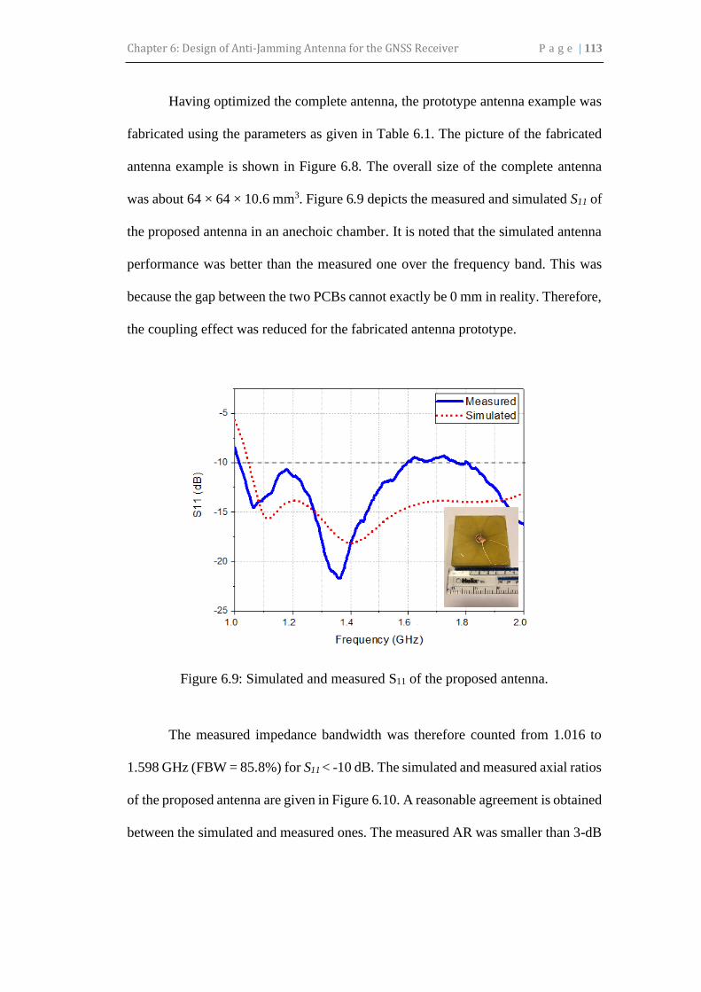
Chapter 6: Design of Anti-Jamming Antenna for the GNSS Receiver P a g e | 113
Having optimized the complete antenna, the prototype antenna example was
fabricated using the parameters as given in Table 6.1. The picture of the fabricated
antenna example is shown in Figure 6.8. The overall size of the complete antenna
was about 64 × 64 × 10.6 mm3. Figure 6.9 depicts the measured and simulated S11 of
the proposed antenna in an anechoic chamber. It is noted that the simulated antenna
performance was better than the measured one over the frequency band. This was
because the gap between the two PCBs cannot exactly be 0 mm in reality. Therefore,
the coupling effect was reduced for the fabricated antenna prototype.
Figure 6.9: Simulated and measured S11 of the proposed antenna.
The measured impedance bandwidth was therefore counted from 1.016 to
1.598 GHz (FBW = 85.8%) for S11 < -10 dB. The simulated and measured axial ratios
of the proposed antenna are given in Figure 6.10. A reasonable agreement is obtained
between the simulated and measured ones. The measured AR was smaller than 3-dB
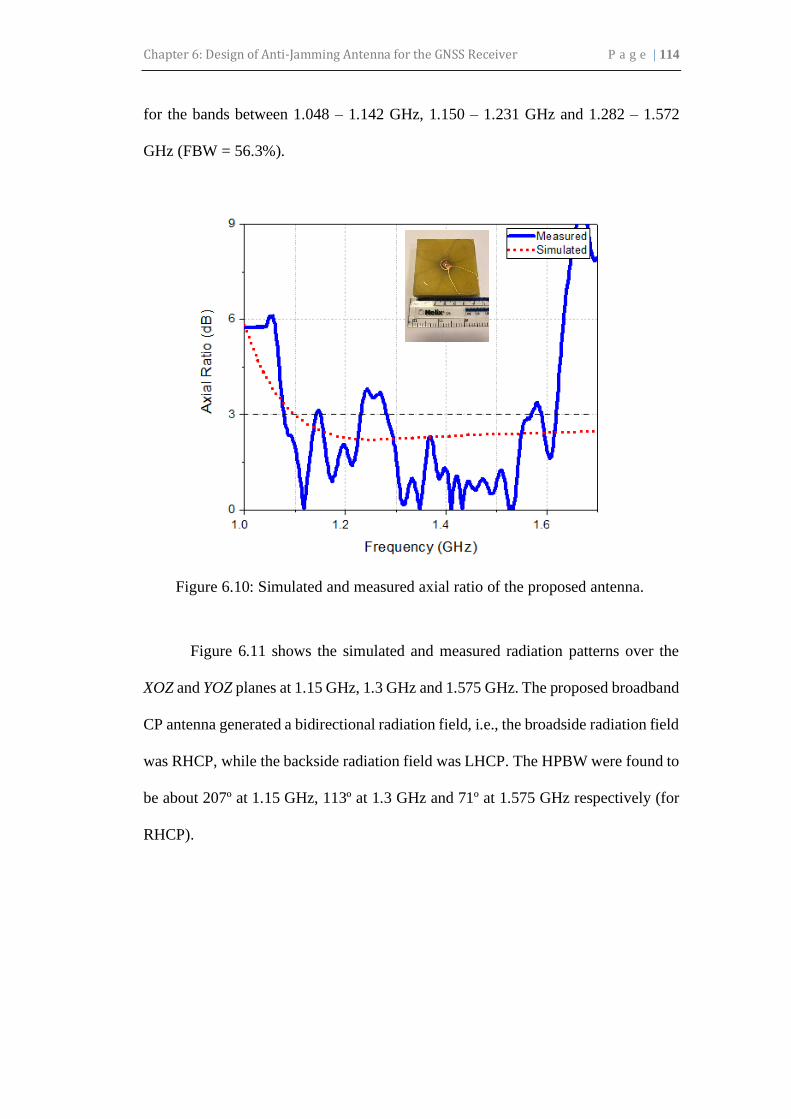
Chapter 6: Design of Anti-Jamming Antenna for the GNSS Receiver P a g e | 114
for the bands between 1.048 – 1.142 GHz, 1.150 – 1.231 GHz and 1.282 – 1.572
GHz (FBW = 56.3%).
Figure 6.10: Simulated and measured axial ratio of the proposed antenna.
Figure 6.11 shows the simulated and measured radiation patterns over the
XOZ and YOZ planes at 1.15 GHz, 1.3 GHz and 1.575 GHz. The proposed broadband
CP antenna generated a bidirectional radiation field, i.e., the broadside radiation field
was RHCP, while the backside radiation field was LHCP. The HPBW were found to
be about 207º at 1.15 GHz, 113º at 1.3 GHz and 71º at 1.575 GHz respectively (for
RHCP).

Chapter 6: Design of Anti-Jamming Antenna for the GNSS Receiver P a g e | 115
(a)
(b)
(c)
Figure 6.11: Simulated and measured radiation pattern over XOZ-plane (left) and
YOZ-plane (right) at three different frequencies. (a) 1.15 GHz. (b) 1.3 GHz. (c)
1.575 GHz.

Chapter 6: Design of Anti-Jamming Antenna for the GNSS Receiver P a g e | 116
Figure 6.12: Simulated and measured axial ratio of the proposed antenna.
The simulated and measured realized gains of the proposed antenna are
shown in Figure 6.12. It can be seen that the gain is around 1 to 3 dBi over the
frequency band of interest. The total efficiency for all frequency band was greater
than 80%.
6.4 ARRAY DESIGN CONFIGURATION
In this section onwards, a new method is proposed to extract the optimal complex
weights for suppression of the jamming signals in a GNSS antenna array. As depicted
in Figure 6.13, the controlled reception pattern antennas (CRPAs), adaptive
antennas, null-steering antennas or beamforming antennas that specialized antenna
that helps protect GNSS receivers from interference and jamming.

Chapter 6: Design of Anti-Jamming Antenna for the GNSS Receiver P a g e | 117
Figure 6.13: CRPA unit is receiving satellite and jammer signals.
The need is, therefore, from the antenna side, to develop miniaturized high-
performance arrays, with reduced footprints, though maintaining as much as possible
the capabilities (i.e., gain and bandwidth) of larger arrays. The quest for small
antennas satisfying both gain and bandwidth requirements has been an active topic
of research over the last decades. Several miniaturization techniques have been
proposed (for a wide review see [138]), with the use of materials having a high
dielectric constant being one of the most common.
Moreover, in order to have a compact system, a total antenna array footprint
miniaturization has to be achieved. The array size has, thus, to shrink, meaning that
the single antennas will be electrically closer to each other. Such aim is by no means
easily achieved, as higher degrees of miniaturization also imply increased mutual
coupling and more difficult antenna matching [139]–[141]. Various efforts to solve
this problem are found in the literature, e.g., by the means of adding a decoupling

Chapter 6: Design of Anti-Jamming Antenna for the GNSS Receiver P a g e | 118
and matching network [142]–[144] able to decouple the coupled patterns of the
antennas, or by using, for instance or split-ring resonators [145]–[147] to limit the
coupling between the elements’ ports. These techniques are, however,
manufacturing-intensive and cannot always be implemented, e.g., due to
requirements on simplicity and versatility.
6.4.1 Antenna Array Configurations and Performances
It is necessary to understand how the design parameters affect antenna performance.
To optimize the antenna performance, some important design parameters and their
effects are studied. There are two designs presented in this section. In the first design,
the five-element array antenna has been proposed (see Figure 6.14). Meanwhile, the
second design which is a four-element array (Figure 6.21) has been proposed to have
a compact system with a good performance.
6.4.1.1 Five-elements array antenna
The geometry of the proposed antenna array is shown in Figure 6.14 and Table 6.2.
The substrate materials for the circuit board is the low-cost FR4 with a relative
permittivity of 4.3 and a thickness of 1.6 mm.
The five elements of the array are placed sequentially rotated with a phase of
0°, 72°, 144°, 216°, and 288°. These sequentially rotated configurations produce a
broad axial ratio bandwidth. The space between two adjacent elements is selected to

Chapter 6: Design of Anti-Jamming Antenna for the GNSS Receiver P a g e | 119
be 80 mm, which is about 0.7 λ0, to minimize mutual coupling without substantial
degradation of the radiation pattern by the sidelobes [148].
(a) (b)
(c)
Figure 6.14: Five-element antenna array configurations (a) perspective view (b) top
view and (c) side view of the antenna.
Table 6.2: Dimension of The Proposed Antenna
Parameter Value (mm) Parameter Value (mm)
Ly 0.5 Lz 8.0
Lx 1.6 Lv 0.5

Chapter 6: Design of Anti-Jamming Antenna for the GNSS Receiver P a g e | 120
The RF signal is fed to a 5-way power divider for each elements array. The
antenna array scanning is simulated using CST Microwave Studio as shown in Figure
6.15. Each of the power divider output is then fed to an individual phase shifter for
each antenna element of each element array where various phase progression was
made to enable beam steering. The phase shifter outputs are finally connected to the
antenna array.
Figure 6.15: Array scanning setup for five elements array in CST MWS.
The antenna array covers the frequency range of 0.974 – 2.342 GHz as shown
in Figure 6.16. The antenna has a total efficiency greater than 90% throughout 0.971
– 2.15 GHz and below 3-dB axial ratio for the entire frequency band as shown in
Figure 6.18 and Figure 6.19.
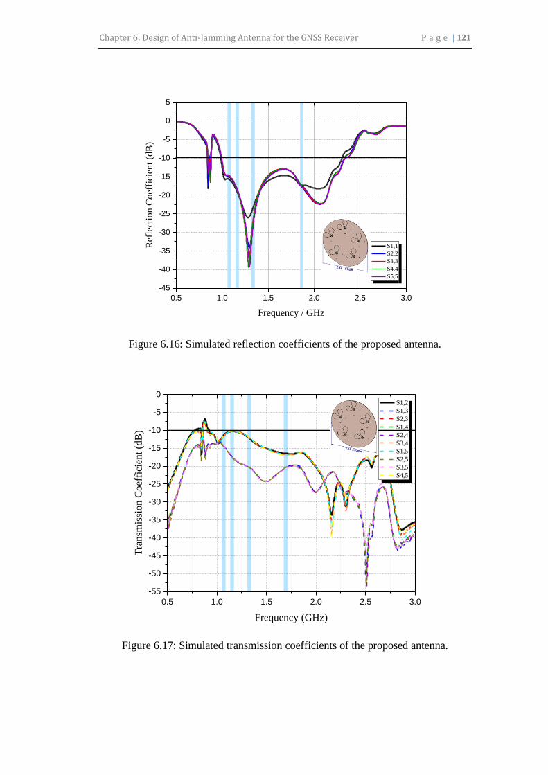
Chapter 6: Design of Anti-Jamming Antenna for the GNSS Receiver P a g e | 121
0.5 1.0 1.5 2.0 2.5 3.0
-45
-40
-35
-30
-25
-20
-15
-10
-5
0
5
S1,1
S2,2
S3,3
S4,4
S5,5
Frequency / GHz
Ref
lect
ion
Co
effi
cien
t (d
B)
Figure 6.16: Simulated reflection coefficients of the proposed antenna.
0.5 1.0 1.5 2.0 2.5 3.0
-55
-50
-45
-40
-35
-30
-25
-20
-15
-10
-5
0 S1,2
S1,3
S2,3
S1,4
S2,4
S3,4
S1,5
S2,5
S3,5
S4,5
Frequency (GHz)
Tra
nsm
issi
on
Co
effi
cien
t (d
B)
Figure 6.17: Simulated transmission coefficients of the proposed antenna.

Chapter 6: Design of Anti-Jamming Antenna for the GNSS Receiver P a g e | 122
Figure 6.18: Simulated axial ratio of the proposed antenna.
1.0 1.1 1.2 1.3 1.4 1.5 1.6 1.7 1.8 1.9 2.0
0.0
0.1
0.2
0.3
0.4
0.5
0.6
0.7
0.8
0.9
1.0
ANT_1
ANT_2
ANT_3
ANT_4
ANT_5
AC1
Frequency (GHz)
To
tal
effi
cien
cy (
*1
00
%)
Figure 6.19: Simulated total efficiency of the proposed antenna.
1.0 1.1 1.2 1.3 1.4 1.5 1.6 1.7 1.8 1.9 2.0
1
2
3
4
5
6 AR_ANT1
AR_ANT2
AR_ANT3
AR_ANT4
AR_ANT5
AR_AC1
Frequency (GHz)
Axia
l R
atio
(dB
)

Chapter 6: Design of Anti-Jamming Antenna for the GNSS Receiver P a g e | 123
1.0 1.1 1.2 1.3 1.4 1.5 1.6 1.7 1.8 1.9 2.0
-4
-2
0
2
4
6
8
10
ANT_1
ANT_2
ANT_3
ANT_4
ANT_5
AC1
Frequency (GHz)
Rea
lize
d G
ain
(d
Bi)
Figure 6.20: Simulated realized gain of the proposed antenna.
6.4.1.2 Four-elements array antenna
To make it more compact, the design is improved by minimizing the number of
element and size of the antenna. In Figure 6.21, the four elements of the 2 × 2 arrays
are placed sequentially rotated with a phase of 0°, 90°, 180°, and 270°. These
sequentially rotated configurations produce a broad axial ratio bandwidth. The space
between two adjacent elements is selected to be 80 mm, which is about 0.7 λ0, to
minimize mutual coupling without substantial degradation of the radiation pattern by
the sidelobes [148].

Chapter 6: Design of Anti-Jamming Antenna for the GNSS Receiver P a g e | 124
(a) (b)
(c)
Figure 6.21: Four-element antenna array configurations (a) perspective view (b) top
view and (c) side view of the antenna.
Table 6.3: Dimension of The Proposed Antenna
Parameter Value (mm) Parameter Value (mm)
Ly 0.5 Lz 8.0
Lx 1.6 Lv 0.5
The antenna array covers the frequency range of 0.959 – 2.333 GHz as shown
in Figure 6.23. The antenna has a total efficiency greater than 90% below 3-dB axial
ratio for the entire frequency bands as shown in Figure 6.24 and Figure 6.25
respectively.

Chapter 6: Design of Anti-Jamming Antenna for the GNSS Receiver P a g e | 125
The RF signal is fed to a 4-way power divider for each elements array. The
antenna array scanning is simulated using CST Microwave Studio as shown in Figure
6.22. Each of the power divider output is then fed to an individual phase shifter for
each antenna element of each element array where various phase progression was
made to enable beam steering. The phase shifter outputs are finally connected to the
antenna array.
Figure 6.22: Array scanning setup for four elements array in CST MWS.

Chapter 6: Design of Anti-Jamming Antenna for the GNSS Receiver P a g e | 126
0.5 1.0 1.5 2.0 2.5 3.0
-30
-25
-20
-15
-10
-5
0
5
S1,1
S2,2
S3,3
S4,4
Frequency (GHz)
Ref
lect
ion
Co
effi
cien
t (d
B)
Figure 6.23: Simulated reflection coefficient of the proposed antenna.
1.0 1.1 1.2 1.3 1.4 1.5 1.6 1.7 1.8 1.9 2.0
0
1
2
3
4
5
6 AR_ANT1
AR_ANT2
AR_ANT3
AR_ANT4
AR_AC1
Frequency (GHz)
Axia
l R
atio
(dB
)
Figure 6.24: Simulated axial ratio of the proposed antenna.

Chapter 6: Design of Anti-Jamming Antenna for the GNSS Receiver P a g e | 127
1.0 1.1 1.2 1.3 1.4 1.5 1.6 1.7 1.8 1.9 2.0
0.0
0.1
0.2
0.3
0.4
0.5
0.6
0.7
0.8
0.9
1.0
ANT1
ANT2
ANT3
ANT4
AC1
Frequency (GHz)
To
tal
effi
cien
cy (
*1
00
%)
Figure 6.25: Simulated total efficiency of the proposed antenna.
1.0 1.1 1.2 1.3 1.4 1.5 1.6 1.7 1.8 1.9 2.0
-4
-2
0
2
4
6
8
10
ANT1
ANT2
ANT3
ANT4
AC1
Frequency (GHz)
Rea
lize
d G
ain
(d
Bi)
Figure 6.26: Simulated total efficiency of the proposed antenna.
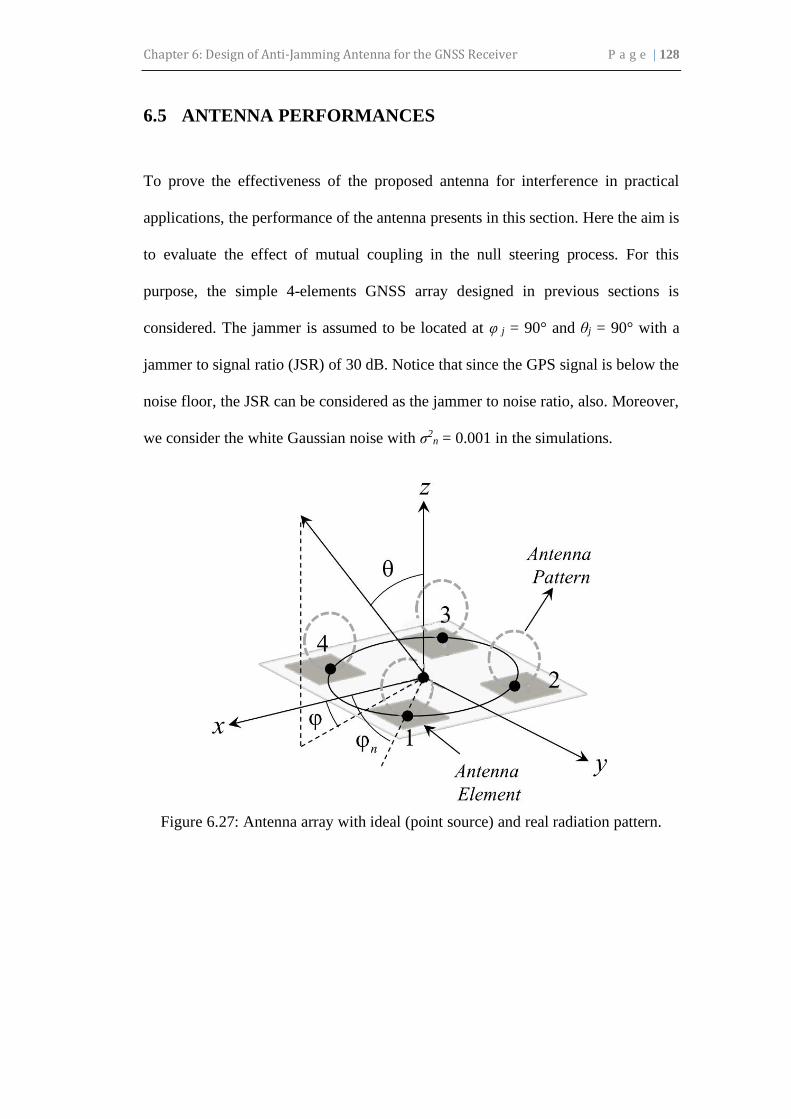
Chapter 6: Design of Anti-Jamming Antenna for the GNSS Receiver P a g e | 128
6.5 ANTENNA PERFORMANCES
To prove the effectiveness of the proposed antenna for interference in practical
applications, the performance of the antenna presents in this section. Here the aim is
to evaluate the effect of mutual coupling in the null steering process. For this
purpose, the simple 4-elements GNSS array designed in previous sections is
considered. The jammer is assumed to be located at φ j = 90° and θj = 90° with a
jammer to signal ratio (JSR) of 30 dB. Notice that since the GPS signal is below the
noise floor, the JSR can be considered as the jammer to noise ratio, also. Moreover,
we consider the white Gaussian noise with σ2n = 0.001 in the simulations.
Figure 6.27: Antenna array with ideal (point source) and real radiation pattern.

Chapter 6: Design of Anti-Jamming Antenna for the GNSS Receiver P a g e | 129
(a)
(b)
Figure 6.28: GPS Antenna array with point sources and real radiation patterns for
SJR=30 dB, SNR=-20 dB and σ = 0.001. The jammer is placed at φj = 90° and θj =
90°. a) φ-plane with θj = 90° b) θ-plane with φj = 90°.

Chapter 6: Design of Anti-Jamming Antenna for the GNSS Receiver P a g e | 130
The results of using these two complex weight vectors are depicted in φ-plane
with θj = 90° (Figure 6.28(a)) and θ-plane with φj = 90° (Figure 6.28(b)). It can be
seen clearly that mutual coupling affects the antenna performance, significantly. In
the real case where the mutual couplings are considered, the jammer signal is
encountered with more than 50 dB null depth, while it is low in the ideal case and
maybe not acceptable. These results clarify the importance of mutual coupling in the
extraction of the complex weight vector.
6.5.1.1 Multi Jammers
As it is well known, an array with N elements can reject N-1 jammer sources.
Therefore, the method with 2, 3 and 4 jammer sources which have the same JSR as
30 dB is evaluated. The jammer sources locations in these three scenarios are
tabulated in Table 6.4, and the corresponding simulation results are shown in Figure
6.30. It can be seen that the proposed method can create a proper null in the direction
of jammer sources to reject their power.
Table 6.4: The Jammer Source Locations in Three Different Scenarios
Jammer Sources
Scenarios
Jammer Source Locations
2- Jammer (20°, 0°), (20°, 300°)
3- Jammer (20°, 0°), (20° ,300°), (60°, 215°)
4- Jammer (20°, 0°), (30° ,90°), (60°, 215°), (20°,300°)

Chapter 6: Design of Anti-Jamming Antenna for the GNSS Receiver P a g e | 131
(a)
(b)
(c)
Figure 6.29: Array patterns after null steering with SJR = 50 dB for different
jammer locations reported in Table 6.4.
(a) 2- jammers (b) 3- jammers (c) 4-jammers.

Chapter 6: Design of Anti-Jamming Antenna for the GNSS Receiver P a g e | 132
(a)
(b)
Figure 6.30: GPS Antenna with different signal to jammer ratio for SNR = -20 dB
and σ = 0.001. The jammer is placed at 𝜑𝑗 = 45° and 𝜃𝑗= 45° (a) φ-plane with 𝜃𝑗 =
45° (b) θ-plane with 𝜑𝑗 = 45°
Moreover, it can be seen that the null depth is highly related to the number of
jammer sources. In other words, the results show that although the null depth is good

Chapter 6: Design of Anti-Jamming Antenna for the GNSS Receiver P a g e | 133
enough in all scenarios, the null depth in the 2-jammer source scenarios is much
higher than the 3 and 4-jammer source. To achieve more null depth with constant
jammer sources, the number of array elements can be increased.
6.5.1.2 Jammer to Signal Effects
Since the proposed method works based on the array minimization, it is expected
that JSR enhancement can help more to recognize the jammer signals from the noise.
To show this fact, one jammer source in 𝜑𝑗 = 45° and 𝜃𝑗 = 45° with three different
JSR as 30, 20 and 10 dB is considered. The simulation results are shown in φ-plane
for 𝜃𝑗 = 45° (Figure 6.30 (a)) and θ-plane for 𝜑𝑗 = 45° (Figure 6.30 (b)). As can be
seen, the null depth is related highly to the JSR. For example, we have about 60 dB
null depth for JSR = 30 dB, while it is about 40 dB for JSR = 20 and only about 25
dB for JSR = 10 dB.
6.6 SUMMARY
This chapter presents a new antenna array configuration combining a 4-elements
antenna array and a 5-elements antenna array to provide wide coverage. The anti-
jamming performance of the antenna with respect to differently polarized jammers
as well as its positioning capability are also presented. All the results have
demonstrated that the antenna is an excellent candidate for the GNSS application.

Chapter 6: Design of Anti-Jamming Antenna for the GNSS Receiver P a g e | 134
An anti-jamming GNSS antenna was designed in this section. The designed
antenna array was formed by four elements antenna in planar array geometry. The
null steering method was performed by using the exact active element patterns of the
array antenna. These patterns include the mutual coupling effect and the nearby
antenna scatterer such as holder which increase the antenna performance to deal with
the jammer sources which was not considered in the literature based on the author
knowledge. Moreover, the proposed method can be easily used in conformal array
structures due to using active antenna pattern in the method. The simulation results
clarified the antenna ability to reject the jammer sources effects.

Chapter 7: Conclusions and Recommendations P a g e | 135
CHAPTER 7:
CONCLUSION AND RECOMMENDATIONS
The overarching questions that this thesis tries to answer are:
1) How to design compact, low profile and yet efficient CP antenna to deliver a
GNSS application with high performance and wide frequency coverage?
2) How to design compact antenna arrays to meet the ever- increasing demand for
wide coverage and wide bandwidth for anti-jamming GNSS applications?
In the first part, this thesis provided an overview of state of the art and extended the
understanding of GNSS systems and fundamentals from an antenna and propagation
perspective to propose and design a new and interesting compact antenna. In the
second part, requirements of the compact GNSS antennas have been analyzed and
various designs have been proposed to achieve these stringent requirements. The
requirements included wide bandwidth, wide coverage, CP capability and low cost

Chapter 7: Conclusions and Recommendations P a g e | 136
of production. In this chapter, the contributions of this thesis to the development of
novel antennas are summarized. Section 7.1 provides a summary of the research
work. The key contributions of this thesis are discussed in Section 7.2. Some
suggestions for future work are discussed in Section 7.3.
7.1 CONCLUSION
This thesis sets out to explore appropriate miniaturization methods for reducing the
size of antennas for GNSS systems. The motivation for this study stems from the
desire to develop a compact GNSS antenna that would provide a broad bandwidth at
GNSS frequency bands which is from 1.1 GHz to 1.6 GHz. CP was desired with an
axial ratio of less than 3dB over each band, with a minimum gain of 0 dBi. Due to
the requirements of bandwidth, CP with the low axial ratio, and gain, many
miniaturization methods fail to meet the required performance.
In Chapter 1, the problem was defined, and the motivation of this research
was discussed. The objectives of the study were defined with the goal of developing
a compact circularly polarized antenna for GNSS applications. In Chapter 2, an
overview of the studies of antennas for target application of GNSS systems been
presented. Some important techniques for anti-jamming have been discussed in
detail.
Following a thorough investigation of the limitations of the existing designs
and understanding the antenna fundamentals, an overview of the current state of the

Chapter 7: Conclusions and Recommendations P a g e | 137
art of the GNSS receiver antenna designs has been introduced in Chapter 3. The
knowledge and prior work presented in this chapter could help readers to understand
state of the art in antenna designs and also realize the research challenges of this
topic. It should be valuable for researchers who are presently working on this topic
and who are going to investigate this area in the near future.
In Chapter 4, the study was focused on the design of a crossed-dipole antenna
with parasitic elements. This broadband antenna demonstrates a significant
improvement on bandwidth and radiation pattern by using the parasitic elements and
loaded monopoles that are excited by coupling with the elliptical crossed dipole in
the center of the antenna. The structure of the antenna is compact and unique. The
dimension of the antenna is 90 mm × 90 mm × 15.5 mm which is small and compact.
The proposed antenna has a bandwidth of 1.06 to 1.671 GHz (611 MHz) for
impedance matching |S11| < -10 dB, and 1.093 to 1.257 GHz (164 MHz) and 1.542
to 1.666 GHz (124 MHz) for an AR < 3-dB. All the results have been demonstrated
that the antenna is an excellent candidate for the GNSS application.
In Chapter 5, a new way of designing a dual-band CP antenna by integrating
a CP radiator with a finite AMC surface were introduced and their application in
protecting dipole antenna from metallic objects was reviewed. The antenna
demonstrates a low-profile broadband characteristic and excellent CP radiation for
GNSS frequency bands. The size of the AMC surface was a crucial factor in defining
the original and additional operating CP bands of the antenna. The measured results
of the proposed design with a size of 100 × 100 × 10 mm3 FR-4 material AMC and
yielded an impedance bandwidth of 1.196 to 2.176 GHz for the |S11|<–10dB and 3-

Chapter 7: Conclusions and Recommendations P a g e | 138
dB AR bandwidths of 1.148 to 1.761 GHz. Meanwhile, the measured results of the
proposed design with a size of 100 × 100 × 12.7 mm3, Rogers RT6006 material AMC
and yielded an impedance bandwidth of 1.153 to 2.36 GHz for the |S11|<–10dB and
3-dB AR bandwidths of 1.170 – 1.970 GHz. Additionally, the proposed antenna
exhibited RHCP and high radiation efficiency (> 90%) in both bands. With a low
profile, broadband characteristics, and high radiation efficiency, the proposed
antenna could be widely applied to dual-band GNSS applications as well as in many
other kinds of satellite communications.
In Chapter 6, this chapter also presents a new antenna array configuration
combining a 4-elements antenna array and a 5-elements antenna array to provide
wide coverage. The anti-jamming performance of the antenna with respect to
differently polarized jammers as well as its positioning capability are also presented.
7.2 LIMITATION AND FUTURE WORK
Based on the conclusions above and considering the limitations of the work existed,
many directions for further improvement and development present themselves. The
following topics provide potential short-term and long-term directions for future
work.
• As these systems become more established and integrated into mainstream
receivers, so will the jammers designed to impede the receivers’
performance. Therefore, it is recommended that this work be expanded in

Chapter 7: Conclusions and Recommendations P a g e | 139
addition to bearing in mind a unified jamming detection platform that
operates on multi-GNSS receivers. Modifications to the methods proposed
in this thesis should be applied when considering other GNSSs, nonetheless,
the approaches and the methodologies followed remain similar. It is
foreseeable that the application of this research to different GNSSs will pose
different challenges depending on the signals under study.
• Decoupling techniques to improve the antenna array isolation needs to be
explored for miniaturization of antenna arrays.
• It is challenging to implement a broadband antenna element in an array
configuration. The spacing between the adjacent antenna elements needs to
be optimized for both the frequency bands. If the antenna element spacing is
set as 0.5 λ for the higher band, the isolation performance for the lower band
becomes poor. If the antenna element spacing is around 0.5 λ for the lower
band, the increase in the grating lobes reduces the realized gain in the higher
band. Using appropriate dummy parasitic elements could be a solution for
this issue and needs further study.
• For the case of a single-element antenna, this could be done by collecting live
data from a differential GNSS receiver and post-processing it in order to
estimate antenna-induced biases. These biases could then be compared to
chamber measurements. This would confirm that the calibration is of
sufficient quality despite environmental effects and other sources of
uncertainty.
• In the case of an antenna array, STAP hardware would be required; however,
it would offer considerable credibility to the proposed approach.

Chapter 7: Conclusions and Recommendations P a g e | 140
The future work in GNSS antenna application is not limited to the works proposed
in this thesis. Vastly broadened spectra and constellations of over 100 MEO and
GEO satellites in GNSS are game-changing events that are reshaping antenna
requirements toward much broader bandwidth and higher cutoff elevation angle.
They pose new challenges not faced by conventional GPS and give rise to new
features and applications as well as cost structures. For size reduction, the slow-wave
technology appears to be a practical solution for applications from handheld to
medium platform but needs considerable research. For pattern control, in particular
higher cutoff angle above horizon, use of metamaterial will be pursued by some,
especially for medium and large platforms. Smart antenna techniques will be
developed to enhance performance in small and handheld platforms in the
increasingly noisier terrestrial environment. There is no doubt an exciting future is
waiting for this technology.

Chapter 7: Conclusions and Recommendations P a g e | 141

References P a g e | 142
[1] B. W. Parkinson, J. J. Spilker, P. Axelrad, P. Enge, and American Institute of
Aeronautics and Astronautics., The Global Positioning System : Theory and
Applications, Volume 1. American Institute of Aeronautics and Astronautics,
1996.
[2] E. Kaplan and C. Hegarty, Understanding GPS Principles and Applications :
Principles and Applications. Artech House, 2005.
[3] P. Misra and P. Enge, Global Positioning System : Signals, Measurements,
and Performance. Ganga-Jamuna Press, 2011.
[4] Wei Liu, Xingqun Zhan, Li Liu, and Mancang Niu, “GNSS RF Compatibility
Assessment: Interference among GPS, Galileo, and Compass : GPS World,”
GPS World, 2010. [Online]. Available: https://www.gpsworld.com/gnss-rf-
compatibility-assessment-10837/.
[5] Thomas A. Stansell, Kenneth W. Hudnut, and Richard G. Keegan, “Future
Wave: L1C Signal Performance and Receiver Design : GPS World,” GPS
World, 2011. [Online]. Available: https://www.gpsworld.com/gnss-
systemgps-modernizationfuture-wave-11401/.
[6] J. J. H. Wang, “Antennas for Global Navigation Satellite System (GNSS),”
Proc. IEEE, vol. 100, no. 7, pp. 2349–2355, Jul. 2012.
[7] Bruce R. Schupler and Thomas A. Clark, “Characterizing the Behavior of
Geodetic GPS Antennas,” GPS World, pp. 48–55, 2001.
[8] A. Kumar, A. D. Sarma, E. Ansari, and K. Yedukondalu, “Improved Phase
Center Estimation for GNSS Patch Antenna,” IEEE Trans. Antennas Propag.,

References P a g e | 143
vol. 61, no. 4, pp. 1909–1915, 2013.
[9] L. Shafai, S. K. Sharma, B. Balaji, A. Damini, and G. Haslam, “Multiple phase
center performance of reflector antennas using a dual mode horn,” IEEE
Trans. Antennas Propag., vol. 54, no. 11, pp. 3407–3417, Nov. 2006.
[10] W. Kunysz, “Antenna phase center effects and measurements in GNSS
ranging applications,” in 2010 14th International Symposium on Antenna
Technology and Applied Electromagnetics and the American
Electromagnetics Conference, ANTEM/AMEREM 2010, 2010.
[11] X. Wang, J. Yao, X. Lu, and W. Lu, “Research on phase center stability of
circularly polarized patch antennas for GPS applications,” in Proceedings of
the 2015 IEEE 4th Asia-Pacific Conference on Antennas and Propagation,
APCAP 2015, 2016, pp. 362–365.
[12] D. M. Pozar, Microwave Engineering, 4th Edition | Wiley, 4th ed. Hoboken,
NJ : Wiley, 2012.
[13] IEEE Antennas and Propagation IEEE Antennas and Propagation Society,
IEEE Standard Definitions of Terms for Antennas. 1993.
[14] C. E. Balanis, Antenna Theory: Analysis and Design, 3rd Edition. 2005.
[15] John D. Kraus, Antennas, 2nd ed. McGraw-Hill, 1988.
[16] H. M. Al-Lawati, “Design and Analysis of Low Profile Circularly Polarised
Antennas,” University of Sheffield, UK, 2014.
[17] J. D. Kraus and R. J. Marhefka, Antennas for All Applications, vol. 1, no. 3rd
Edition. 2002.
[18] S. S. Gao; Q. Luo; F. Zhu, Circularly Polarized Antennas. Chichester, West
Sussex: John Wiley & Sons, Ltd, 2014.
[19] Y. Huang and K. Boyle, Antennas : From Theory to Practice. John Wiley &

References P a g e | 144
Sons, 2008.
[20] W. Kunysz, “Effect of Antenna Performance on the GPS Signal Accuracy,”
in Proceedings of the 1998 National Technical Meeting of The Institute of
Navigation, 1998, pp. 575–580.
[21] G. J. K. Moernaut and D. Orban, “GNSS Antennas An Introduction to
Bandwidth, Gain Pattern, Polarization, and All That,” GPS World, pp. 42–48,
2009.
[22] D. B. Thornberg, D. S. Thornberg, M. F. Dibenedetto, M. S. Braasch, F. Van
Graas, and C. Bartone, “LAAS Integrated Multipath-Limiting Antenna,” J.
Inst. Navig., vol. 50, no. 2, pp. 117–130, Jun. 2003.
[23] M. Braasch, “Optimum Antenna Design for DGPS Ground Reference
Stations,” in Proceedings of the 7th International Technical Meeting of the
Satellite Division of The Institute of Navigation (ION GPS 1994), 1994, pp.
1291–1297.
[24] I. M. Barton, “Antenna Performance Analysis for The Nationwide Differential
Global Positioning System,” Ohio University, 2005.
[25] F. van Graas, C. Bartone, and T. Arthur, “GPS Antenna Phase and Group
Delay Corrections,” in Proceedings of the 2004 National Technical Meeting
of The Institute of Navigation, 2004, pp. 399–408.
[26] L. J. Chu, “Physical Limitations of Omni‐Directional Antennas,” J. Appl.
Phys., vol. 19, no. 12, pp. 1163–1175, Dec. 1948.
[27] R. C. Johnson and H. Jasik, Antenna Engineering Handbook. McGraw-Hill,
1984.
[28] C. A. Balanis, Modern Antenna Handbook. Wiley, 2011.
[29] C.-C. Chen, S. S. Gao, and M. Maqsood, “Antennas for Global Navigation

References P a g e | 145
Satellite System Receivers,” in Space Antenna Handbook, Chichester, UK:
John Wiley & Sons, Ltd, 2012, pp. 548–595.
[30] B. R. Rao, W. Kunysz, R. Fante, and K. McDonald, GPS/GNSS Antennas.
Artech House, 2012.
[31] J. J. H. Wang, “The Spiral as a Traveling Wave Structure for Broadband
Antenna Applications,” Electromagnetics, vol. 20, no. 4, pp. 323–342, Jul.
2000.
[32] J. J. H. Wang and D. J. Triplett, “High-performance Universal GNSS Antenna
and Enhancement Techniques to Overcome Its Performance Limitations,” in
2010 IEEE Antennas and Propagation Society International Symposium,
2010, pp. 1–4.
[33] “Official U.S. government information about the Global Positioning System
(GPS) and related topics.” [Online]. Available:
https://www.gps.gov/systems/gps/space/.
[34] G. Xu, GPS : Theory, Algorithms, and Applications. Springer, 2007.
[35] J. Farrell and M. Barth, The Global Positioning System and Inertial
Navigation. McGraw-Hill, 1999.
[36] D. Doberstein, Fundamentals of GPS Receivers : A Hardware Approach.
Springer, 2012.
[37] “GLONASS Interface Control Document (ICD),” 2002. [Online]. Available:
http://www.glonass-ianc.rsa.ru/.
[38] “IEEE Standard Test Procedures for Antennas,” ANSI/IEEE Std 149-1979,
1979. [Online]. Available: doi: 10.1109/IEEESTD.1979.120310.
[39] L. Musumeci and F. Dovis, “Use of the Wavelet Transform for Interference
Detection and Mitigation in Global Navigation Satellite Systems,” Int. J.

References P a g e | 146
Navig. Obs., vol. 2014, pp. 1–14, Feb. 2014.
[40] R. Bauernfeind, T. Kraus, A. S. Ayaz, D. Dötterböck, and B. Eissfeller,
“Analysis, Detection and Mitigation of In Car GNSS Jammer Interference Inn
Intelligent Transport Systems,” in Deutscher Luft- und Raumfahrtkongress
2012, 2012, pp. 1–10.
[41] D. Borio, C. O’Driscoll, and J. Fortuny, “GNSS Jammers: Effects and
Countermeasures,” in 2012 6th ESA Workshop on Satellite Navigation
Technologies (Navitec 2012) & European Workshop on GNSS Signals and
Signal Processing, 2012, pp. 1–7.
[42] Michael Jones, “The Civilian Battlefield: Protecting GNSS Receivers from
Interference and Jamming,” Inside GNSS, pp. 40–49, 2011.
[43] M. Marcus, “Growing Consumer Interest in Jamming: Spectrum Policy
Implications [Spectrum Policy and Regulatory Issues],” IEEE Wirel.
Commun., vol. 21, no. 1, pp. 4–4, Feb. 2014.
[44] A. Georgiadis, Microwave and Millimeter Wave Circuits and Systems :
Emerging Design, Technologies and Aapplications. John Wiley & Sons,
2012.
[45] D. Borio, C. O’Driscoll, and J. Fortuny, “Jammer Impact on Galileo and GPS
Receivers,” in 2013 International Conference on Localization and GNSS
(ICL-GNSS), 2013, pp. 1–6.
[46] M. Moussa, “High Resolution Jamming Detection in Global Navigation
Satellite Systems,” Queen’s University Kingston, Ontario, Canada, 2015.
[47] Emily McMilin, “Single Antenna Null-Steering for GPS & GNSS Aerial
Applications,” Stanford University, 2016.
[48] S. D. A, “GNSS Interference Mitigation Using Antenna Array Processing,”

References P a g e | 147
University of Calgary, Aberta, 2013.
[49] S. Deshpande, “Study of Interference Effects on GPS Signal Acquisition,”
University of Calgary, 2004.
[50] B. D. Van Veen and K. M. Buckley, “Beamforming: A Versatile Approach to
Spatial Filtering,” IEEE ASSP Mag., vol. 5, no. 2, pp. 4–24, Apr. 1988.
[51] J. Li, “GPS Interference Mitigation for Small UAV Applications,” The
University of Adelaide, 2009.
[52] M. Trinkle and D. Gray, “GPS Interference Mitigation; Overview and
Experimental Results,” in 5th International Symposium on Satellite
Navigation Technology & Applications, 2001.
[53] Wang Lijun and Miao Huanping, “The System Model and Analysis of All-
Digital Temporal and Spatial Anti-jamming for GPS Receivers,” in IET 3rd
International Conference on Wireless, Mobile and Multimedia Networks
(ICWMMN 2010), 2010, pp. 258–261.
[54] C. Xue, H. Wang, X. Jiang, and Y. Huang, “A Single-Feed Arrow-Shaped
Circularly Polarized Antenna With Unbalanced Slotted Artificial Magnetic
Conductor for GNSS Application,” in 2016 IEEE MTT-S International
Microwave Workshop Series on Advanced Materials and Processes for RF
and THz Applications (IMWS-AMP), 2016, pp. 4–6.
[55] S. X. Ta, J. J. Han, I. Park, and R. W. Ziolkowski, “Wide-Beam Circularly
Polarized Crossed Scythe-Shaped Dipoles for Global Navigation Satellite
Systems,” J. Electromagn. Eng. Sci., vol. 13, no. 4, pp. 224–232, 2013.
[56] S. X. Ta, H. Choo, I. Park, and R. W. Ziolkowski, “Multi-Band, Wide-Beam,
Circularly Polarized, Crossed, Asymmetrically Barbed Dipole Antennas for
GPS Applications,” IEEE Trans. Antennas Propag., vol. 61, no. 11, pp. 5771–

References P a g e | 148
5775, Nov. 2013.
[57] S. X. Ta and I. Park, “Crossed Dipole Loaded With Magneto-Electric Dipole
for Wideband and Wide-Beam Circularly Polarized Radiation,” IEEE
Antennas Wirel. Propag. Lett., vol. 14, pp. 358–361, 2015.
[58] J.-W. W. Baik, T.-H. H. Lee, S. Pyo, S.-M. M. Han, J. Jeong, and Y.-S. S.
Kim, “Broadband Circularly Polarized Crossed Dipole with Parasitic Loop
Resonators and Its Arrays,” IEEE Trans. Antennas Propag., vol. 59, no. 1, pp.
80–88, Jan. 2011.
[59] S. Hu, X. Chen, and D. Zhao, “Novel Compact Monopole Antennas for Global
Navigation Satellite Systems,” in 2015 IEEE 4th Asia-Pacific Conference on
Antennas and Propagation (APCAP), 2015, pp. 210–211.
[60] Y. Cao, S. W. Cheung, and T. I. Yuk, “A Simple Planar Polarization
Reconfigurable Monopole Antenna for GNSS/PCS,” IEEE Trans. Antennas
Propag., vol. 63, no. 2, pp. 500–507, Feb. 2015.
[61] R. Xu, J.-Y. Li, and W. Kun, “A Broadband Circularly Polarized Crossed-
Dipole Antenna,” IEEE Trans. Antennas Propag., vol. 64, no. 10, pp. 4509–
4513, Oct. 2016.
[62] A. Selek, C. Turkmen, and M. Secmen, “Compact planar folded monopole
antenna with coupling mechanism for Quad ISM band, GNSS and UMTS
applications,” in GeMiC 2018 - 2018 German Microwave Conference, 2018,
vol. 2018-January, pp. 211–214.
[63] G. B. Abdelsayed, S. I. Shams, and a. M. M. a Allam, “Triple-band Circularly
Polarized Slotted Patch Antenna for GPS and UMTS Systems,” in 2010 10th
Mediterranean Microwave Symposium, MMS 2010, 2010, pp. 448–451.
[64] C. Chen, X. Zhang, S. Qi, and W. Wu, “Wideband Circular Polarization

References P a g e | 149
Cavity-Backed Slot Antenna for GNSS Applications,” Prog. Electromagn.
Res. Lett., vol. 52, no. February, pp. 31–36, 2015.
[65] Nasimuddin, X. Qing, and Z. N. Chen, “A Compact Circularly Polarized
Slotted Patch Antenna for GNSS Applications,” IEEE Trans. Antennas
Propag., vol. 62, no. 12, pp. 6506–6509, Dec. 2014.
[66] S. B. Sharma, A. Ugle, and K. Parikh, “A Novel U-slot Aperture Coupled
Annular-Ring Microstrip Patch Antenna for Multiband GNSS Applications,”
in 14th European Conference on Antennas and Propagation, EuCAP 2020,
2020.
[67] Nasimuddin and X. Qing, “A Single-feed Compact Wideband Circularly
Polarized Antenna for INMARSAT/GNSS Applications,” in 14th European
Conference on Antennas and Propagation, EuCAP 2020, 2020.
[68] H. Zhang, Y. Guo, and G. Wang, “A Wideband Circularly Polarized Crossed-
Slot Antenna with Stable Phase Center,” IEEE Antennas Wirel. Propag. Lett.,
vol. 18, no. 5, pp. 941–945, May 2019.
[69] A. Alphones, K. Agarwal, and Nasimuddin, “Triple-band Compact Circularly
Polarised Stacked Microstrip Antenna Over Reactive Impedance Meta-
surface for GPS Applications,” IET Microwaves, Antennas Propag., vol. 8,
no. 13, pp. 1057–1065, 2014.
[70] O. P. Falade, M. U. Rehman, Y. Gao, X. Chen, and C. G. Parini, “Single Feed
Stacked Patch Circular Polarized Antenna for Triple Band GPS Receivers,”
IEEE Trans. Antennas Propag., vol. 60, no. 10, pp. 4479–4484, 2012.
[71] J. M. Baracco, L. Salghetti-Drioli, and P. de Maagt, “AMC Low Profile
Wideband Reference Antenna for GPS and GALILEO Systems,” IEEE Trans.
Antennas Propag., vol. 56, no. 8 II, pp. 2540–2547, 2008.

References P a g e | 150
[72] Moran Wang, Xiaoqiao Deng, and Changqing Gu, “Tri-band GPS Antenna
with Low-Multipath Ground Plane,” in 2010 International Symposium on
Signals, Systems and Electronics, 2010, vol. 2, pp. 1–4.
[73] U. U. Hussine, M. T. Islam, and N. Misran, “A New I Slotted Compact
Microstrip Antenna for L1 & L2 Bands,” in 2011 IEEE International
Conference on Space Science and Communication, 2011, pp. 286–290.
[74] N. Rezazadeh and L. Shafai, “A Compact Microstrip Patch Antenna for
Civilian GPS Interference Mitigation,” IEEE Antennas Wirel. Propag. Lett.,
vol. 6, no. c, pp. 7–10, 2018.
[75] M. Khalily, M. K. a Rahim, and A. a. Kishk, “Planar Wideband Circularly
Polarized Antenna Design with Rectangular Ring Dielectric Resonator and
Parasitic Printed Loops,” IEEE Antennas Wirel. Propag. Lett., vol. 11, pp.
905–908, 2012.
[76] H. Nguyen-bich, H. Chu-ba, and C. Dao-ngoc, “All GPS Bands Dielectric
Resonator Antenna with Circular Polarization for GPS Application,” in The
2012 International Conference on Advanced Technologies for
Communications, 2012, pp. 65–68.
[77] G. Massie, M. Caillet, M. Clénet, and Y. M. M. Antar, “A New Wideband
Circularly Polarized Hybrid Dielectric Resonator Antenna,” IEEE Antennas
Wirel. Propag. Lett., vol. 9, pp. 347–350, 2010.
[78] S. Jovic, M. Clenet, and M. M. Yahia Antar, “Novel Wideband Antenna for
GNSS and Satellite Communications,” in 14th European Conference on
Antennas and Propagation, EuCAP 2020, 2020.
[79] G. Mazingue, B. Byrne, M. Romier, and N. Capet, “3D Printed Ceramic
Antennas for Space Applications,” in 14th European Conference on Antennas

References P a g e | 151
and Propagation, EuCAP 2020, 2020.
[80] A. Sharma, G. Das, S. Gupta, and R. K. Gangwar, “Quad-Band Quad-Sense
Circularly Polarized Dielectric Resonator Antenna for
GPS/CNSS/WLAN/WiMAX Applications,” IEEE Antennas Wirel. Propag.
Lett., vol. 19, no. 3, pp. 403–407, Mar. 2020.
[81] U. Illahi, J. Iqbal, M. I. Sulaiman, M. Alam, M. S. Mazliham, and M. H.
Jamaluddin, “A Conformal Metal Strip Fed Circularly Polarized Rectangular
Dielectric Resonator Antenna,” in APACE 2019 - 2019 IEEE Asia-Pacific
Conference on Applied Electromagnetics, Proceedings, 2019.
[82] Y. Liu, Y. Jiao, Z. Weng, C. Zhang, and H. Zhang, “A high-gain dielectric
resonator antenna array fed by back-cavity,” in 2018 IEEE International
Workshop on Antenna Technology, iWAT2018 - Proceedings, 2018, pp. 1–3.
[83] Son Xuat Ta, Ikmo Park, and R. W. Ziolkowski, “Crossed Dipole Antennas:
A review,” IEEE Antennas and Propagation Magazine, vol. 57, no. 5. IEEE
Computer Society, pp. 107–122, 01-Oct-2015.
[84] L. Zhang et al., “Single-Feed Ultra-Wideband Circularly Polarized Antenna
With Enhanced Front-to-Back Ratio,” IEEE Trans. Antennas Propag., vol.
64, no. 1, pp. 355–360, Jan. 2016.
[85] J. A. Kasemodel, C.-C. Chen, I. J. Gupta, and J. L. Volakis, “Miniature
Continuous Coverage Antenna Array for GNSS Receivers,” IEEE Antennas
Wirel. Propag. Lett., vol. 7, pp. 592–595, 2008.
[86] R. Joshi et al., “Dual-Band, Dual-Sense Textile Antenna with AMC Backing
for Localization Using GPS and WBAN/WLAN,” IEEE Access, vol. 8, pp.
89468–89478, 2020.
[87] A. J. OBrien and I. J. Gupta, “Mitigation of Adaptive Antenna Induced Bias

References P a g e | 152
Errors in GNSS Receivers,” IEEE Trans. Aerosp. Electron. Syst., vol. 47, no.
1, pp. 524–538, Jan. 2011.
[88] Y. Zhou, C. Chen, and J. L. Volakis, “Single-fed Circularly Polarized Antenna
Element with Reduced Coupling for GPS Arrays,” IEEE Trans. Antennas
Propag., vol. 56, no. 5, pp. 1469–1472, 2008.
[89] M. Chen and C. C. Chen, “A Compact Dual-band GPS Antenna Design,”
IEEE Antennas Wirel. Propag. Lett., vol. 12, pp. 245–248, 2013.
[90] Y. Zhou, C.-C. Chen, and J. L. Volakis, “A Compact 4-Element Dual-band
GPS Array,” in 2009 IEEE Antennas and Propagation Society International
Symposium, 2009, pp. 1–4.
[91] B. A. Kramer, M. Lee, C.-C. Chen, and J. L. Volakis, “A Miniature Conformal
Spiral Antenna Using Inductive and Dielectric Loading,” in 2007 IEEE
Antennas and Propagation International Symposium, 2007, pp. 1004–1007.
[92] Y. Zhou, S. Koulouridis, G. Kiziltas, and J. L. Volakis, “A Novel 1.5"
Quadruple Antenna for Tri-Band GPS Applications,” IEEE Antennas Wirel.
Propag. Lett., vol. 5, pp. 224–227, 2006.
[93] A. S. C. Svendsen and I. J. Gupta, “Adaptive Antenna for Handheld GPS
Receivers,” in IEEE/ION Position, Location and Navigation Symposium,
2010, pp. 436–442.
[94] H. Sedighy, “Null Steering GPS Array in the Presence of Mutual Coupling,”
Iran. J. Electr. Electron. Eng., vol. 14, no. 2, pp. 116–123, 2018.
[95] S. X. Ta, H. H. Tran, and I. Park, “Wideband Circularly Polarized Antenna
for GNSS Applications,” in 2014 IEEE Conference on Antenna
Measurements & Applications (CAMA), 2014, pp. 1–3.
[96] M. A. Fiddy and R. Tsu, “Understanding metamaterials,” Waves in Random

References P a g e | 153
and Complex Media, vol. 20, no. 2, pp. 202–222, May 2010.
[97] Fan Yang and Y. Rahmat-Samii, “Reflection Phase Characterizations of the
EBG Ground Plane for Low Profile Wire Antenna Applications,” IEEE Trans.
Antennas Propag., vol. 51, no. 10, pp. 2691–2703, Oct. 2003.
[98] D. Sievenpiper, L. Zhang, R. F. Jimenez Broas, N. G. Alexöpolous, and E.
Yablonovitch, “High-impedance electromagnetic surfaces with a forbidden
frequency band,” IEEE Trans. Microw. Theory Tech., vol. 47, no. 11, pp.
2059–2074, 1999.
[99] S. Clavijo, R. E. Diaz, and W. E. McKinzie, “Design Methodology for
Sievenpiper High-Impedance Surfaces: An Artificial Magnetic Conductor for
Positive Gain Electrically Small Antennas,” IEEE Trans. Antennas Propag.,
vol. 51, no. 10, pp. 2678–2690, Oct. 2003.
[100] H. Mosallaei and K. Sarabandi, “Antenna Miniaturization and Bandwidth
Enhancement Using a Reactive Impedance Substrate,” IEEE Trans. Antennas
Propag., vol. 52, no. 9, pp. 2403–2414, Sep. 2004.
[101] S. Zhu and R. Langley, “Dual-Band Wearable Textile Antenna on an EBG
Substrate,” IEEE Trans. Antennas Propag., vol. 57, no. 4, pp. 926–935, Apr.
2009.
[102] O. Folayan and R. Langley, “Dual Frequency Band Antenna Combined with
A High Impedance Band Gap Surface,” IET Microwaves, Antennas Propag.,
vol. 3, no. 7, p. 1118, 2009.
[103] N. A. Abbasi and R. J. Langley, “Multiband-Integrated Antenna/Artificial
Magnetic Conductor,” IET Microwaves, Antennas Propag., vol. 5, no. 6, p.
711, 2011.
[104] D. Chen, W. Yang, W. Che, Q. Xue, and L. Gu, “Polarization-Reconfigurable

References P a g e | 154
and Frequency-Tunable Dipole Antenna Using Active AMC Structures,”
IEEE Access, vol. 7, pp. 77792–77803, 2019.
[105] E. George and C. Saha, “An AMC Backed Slotted Ground Antenna for
Broadside Radiation and High Gain,” in Proceedings of the 2019 IEEE Recent
Advances in Geoscience and Remote Sensing: Technologies, Standards and
Applications, TENGARSS 2019, 2019, pp. 61–63.
[106] H. Yi and S.-W. Qu, “A Novel Dual-Band Circularly Polarized Antenna
Based on Electromagnetic Band-Gap Structure,” IEEE Antennas Wirel.
Propag. Lett., vol. 12, pp. 1149–1152, 2013.
[107] D. Qu, L. Shafai, and A. Foroozesh, “Improving microstrip patch antenna
performance using EBG substrates,” IEE Proc. Microwaves, Antennas
Propag., vol. 153, no. 6, pp. 558–563, 2006.
[108] D. N. Elsheakh, H. A. Elsadek, E. A. Abdallah, H. Elhenawy, and M. F.
Iskander, “Enhancement of microstrip monopole antenna bandwidth by using
EBG structures,” IEEE Antennas Wirel. Propag. Lett., vol. 8, pp. 959–962,
2009.
[109] W. Wan, Q. Wang, and T. Ye, “Research of Low-profile High Performance
new AMC Antenna for 5G mm-Wave AiP Application,” in 2019 20th
International Conference on Electronic Packaging Technology, ICEPT 2019,
2019.
[110] M. Xue, W. Wan, Q. Wang, and L. Cao, “Wideband Low-Profile Ka-Band
Microstrip Antenna with Low Cross Polarization Using Asymmetry AMC
Structure,” in Proceedings - Electronic Components and Technology
Conference, 2019, pp. 2318–2323.
[111] M. E. de Cos, Y. Álvarez, and F. Las-Heras, “On The Influence of Coupling

References P a g e | 155
AMC Resonances for RCS Reduction in The SHF Band,” Prog. Electromagn.
Res., vol. 117, pp. 103–119, 2011.
[112] C. C. Chiau, X. Chen, and C. Parini, “Multiperiod EBG Structure for Wide
Stopband Circuits,” IEE Proc. Microwaves, Antennas Propag., vol. 150, no.
6, pp. 489–492, Dec. 2003.
[113] L. Akhoondzadeh-Asl, “Wideband Dipoles on Electromagnetic Bandgap
Ground Planes,” in IEE Wideband and Multi-band Antennas and Arrays 2005,
2006, pp. 41–45.
[114] Y. Zhang, J. Von Hagen, M. Younis, C. Fischer, and W. Wiesbeck, “Planar
Artificial Magnetic Conductors and Patch Antennas,” IEEE Trans. Antennas
Propag., vol. 51, no. 10, pp. 2704–2712, 2003.
[115] A. P. Feresidis, G. Goussetis, S. Wang, and J. C. Vardaxoglou, “Artificial
magnetic conductor surfaces and their application to low-profile high-gain
planar antennas,” IEEE Trans. Antennas Propag., vol. 53, no. 1 I, pp. 209–
215, Jan. 2005.
[116] S. Wang, A. P. Feresidis, G. Goussetis, and J. C. Vardaxoglu, “Low-Profile
Resonant Cavity Antenna with Artificial Magnetic Conductor Ground Plane,”
Electron. Lett., vol. 40, no. 7, pp. 405–406, Apr. 2004.
[117] S. H. Kim, T. T. Nguyen, and J. H. Jang, “Reflection Characteristics of 1-D
EBG Ground Plane and Its Application to A Planar Dipole Antenna,” Prog.
Electromagn. Res., vol. 120, pp. 51–66, 2011.
[118] L. Li et al., “Frequency-Reconfigurable Quasi-Sierpinski Antenna Integrating
with Dual-Band High-Impedance Surface,” IEEE Trans. Antennas Propag.,
vol. 62, no. 9, pp. 4459–4467, Sep. 2014.
[119] E. J. Rothwell and R. O. Ouedraogo, “Antenna Miniaturization: Definitions,

References P a g e | 156
Concepts, and A Review with Emphasis on Metamaterials,” J. Electromagn.
Waves Appl., vol. 28, no. 17, pp. 2089–2123, Nov. 2014.
[120] J. McVay, N. Engheta, and A. Hoorfar, “High Impedance Metamaterial
Surfaces Using Hilbert-Curve Inclusions,” IEEE Microw. Wirel. Components
Lett., vol. 14, no. 3, pp. 130–132, Mar. 2004.
[121] G. Goussetis, A. P. Feresidis, and J. C. Vardaxoglou, “Tailoring the AMC and
EBG Characteristics of Periodic Metallic Arrays Printed on Grounded
Dielectric Substrate,” IEEE Trans. Antennas Propag., vol. 54, no. 1, pp. 82–
89, 2006.
[122] S. B. Glybovski, S. A. Tretyakov, P. A. Belov, Y. S. Kivshar, and C. R.
Simovski, “Metasurfaces: From Microwaves to Visible,” Elsevier B.V., May
2016.
[123] R. Dewan, S. K. A. Rahim, F. Malek, S. F. Ausordin, A. A. Yusuf, and S. N.
Azemi, “A Dual-Band Array Antenna Using Dome-Shaped Radiating
Patches,” Microw. Opt. Technol. Lett., vol. 55, no. 11, pp. 2680–2686, Nov.
2013.
[124] R. T. Ioannides, T. Pany, and G. Gibbons, “Known Vulnerabilities of Global
Navigation Satellite Systems, Status, and Potential Mitigation Techniques,”
Proc. IEEE, vol. 104, no. 6, pp. 1174–1194, 2016.
[125] A. Pinker and C. Smith, “Vulnerability of the GPS Signal to Jamming,” GPS
Solutions, vol. 3, no. 2, Wiley, pp. 19–27, Oct-1999.
[126] M. M. Casabona and M. W. Rosen, “Discussion of GPS Anti-Jam
Technology,” GPS Solutions, vol. 2, no. 3, Wiley, pp. 18–23, Jan-1999.
[127] A. Konovaltsev, D. S. De Lorenzo, A. Hornbostel, and P. K. Enge,
“Mitigation of Continuous and Pulsed Radio Interference with GNSS Antenna

References P a g e | 157
Arrays,” in Proceedings of the 21st International Technical Meeting of the
Satellite Division of The Institute of Navigation (ION GNSS 2008), 2008, pp.
2786–2795.
[128] Y. Guo, M. Fan, X. DIng, F. Yan, W. Xie, and M. Kong, “Analysis and
Application of CNR Performance of STAP Anti-Jamming Method for GNSS
Receiver,” in ICSIDP 2019 - IEEE International Conference on Signal,
Information and Data Processing 2019, 2019.
[129] X. Yang, F. Chen, W. Liu, and F. Wang, “Analysis of the Effect Jammer
Types on GNSS Receiver Measurements,” in 2019 2nd IEEE International
Conference on Information Communication and Signal Processing, ICICSP
2019, 2019, pp. 117–120.
[130] T. E. Humphreys, B. M. Ledvina, M. L. Psiaki, B. W. O’Hanlon, P. M.
Kintner, and Jr., “Assessing the Spoofing Threat: Development of a Portable
GPS Civilian Spoofer,” in Proceedings of the 21st International Technical
Meeting of the Satellite Division of The Institute of Navigation (ION GNSS
2008), 2008, pp. 2314–2325.
[131] B. M. Ledvina, W. J. Bencze, B. Galusha, and I. Miller, “An In-Line Anti-
Spoofing Device for Legacy Civil GPS Receivers,” in Proceedings of the
2010 International Technical Meeting of The Institute of Navigation, 2010,
pp. 698–712.
[132] Randolph G. Hartman, “US5557284A: Spoofing Detection System for A
Satellite Positioning System,” 03-Feb-1995.
[133] M. L. Psiaki, S. P. Powell, and B. W. O’Hanlon, “GNSS Spoofing Detection
using High-Frequency Antenna Motion and Carrier-Phase Data,” in
Proceedings of the 26th International Technical Meeting of the Satellite

References P a g e | 158
Division of The Institute of Navigation (ION GNSS+ 2013), 2013, pp. 2949–
2991.
[134] S. Daneshmand, A. Jafarnia-Jahromi, A. Broumandon, and G. Lachapelle, “A
Low-Complexity GPS Anti-Spoofing Method Using a Multi-Antenna Array,”
in Proceedings of the 25th International Technical Meeting of the Satellite
Division of The Institute of Navigation (ION GNSS 2012), 2012, pp. 1233–
1243.
[135] T. Humphreys, J. Bhatti, D. Shepard, and K. Wesson, “A Testbed for
Developing and Evaluating GNSS Signal Authentication Techniques,” in
Proc. Int. Symp. Certification of GNSS Systems Services (CERGAL), 2014,
pp. 1–5.
[136] J. L. Volakis, A. J. O’Brien, and C.-C. Chen, “Small and Adaptive Antennas
and Arrays for GNSS Applications,” in Proceedings of the IEEE, 2016, vol.
104, no. 6, pp. 1221–1232.
[137] C. Song, Y. Huang, Q. Xu, and U. U. Hussine, “A Broadband Circularly
Polarized Cross-dipole Antenna for GNSS Applications,” in 2015
Loughborough Antennas and Propagation Conference, LAPC 2015, 2015.
[138] J. L. Volakis, C.-C. Chen, and K. (Kyohei) Fujimoto, Small Antennas :
Miniaturization Techniques Applications. McGraw-Hill, 2010.
[139] S. Caizzone and A. Dreher, “An Uncoupled Rematching Technique for
Coupled Receive Arrays,” in Microwave Conference (GeMIC), 2014, pp. 1–
3.
[140] H. Y. Yuan et al., “Dual-Band Dual-Polarized Microstrip Antenna for
Compass Navigation Satellite System,” Prog. Electromagn. Res. C, vol. 30,
pp. 213–223, 2012.

References P a g e | 159
[141] C. Martel, “Low profile and anti-jam GPS array,” in IEEE Antennas and
Propagation Society, AP-S International Symposium (Digest), 2013, pp.
1216–1217.
[142] Maysam Ibraheam, S. Irteza, S. Caizzone, A. Dreher, R. Stephan, and M. A.
Hein, “Compact Dual-band Dual-Polarized Antenna Array for Robust
Satellite Navigation Receivers,” in 2015 9th European Conference on
Antennas and Propagation (EuCAP), 2015.
[143] C. Volmer, J. Weber, R. Stephan, K. Blau, and M. A. Hein, “An Eigen-
Analysis of Compact Antenna Arrays and Its Application to Port
Decoupling,” IEEE Trans. Antennas Propag., vol. 56, no. 2, pp. 360–370,
2008.
[144] X. Shao et al., “Compact Triple Band Antenna Array for GNSS Application,”
in 2016 IEEE International Conference on Microwave and Millimeter Wave
Technology (ICMMT), 2016, pp. 1–3.
[145] A. A. Gheethan, P. A. Herzig, and G. Mumcu, “Compact 2 x 2 Coupled
Double Loop GPS Antenna Array Loaded With Broadside Coupled Split Ring
Resonators,” IEEE Trans. Antennas Propag., vol. 61, no. 6, pp. 3000–3008,
Jun. 2013.
[146] K. N. Paracha et al., “A Low Profile, Dual-band, Dual Polarized Antenna for
Indoor/Outdoor Wearable Application,” IEEE Access, vol. 7, pp. 33277–
33288, 2019.
[147] C. Abdelhamid, M. Daghari, H. Sakli, and C. Hamrouni, “A new UWB-
MIMO Multi-Antennas with High Isolation for Satellite Communications,” in
2019 15th International Wireless Communications and Mobile Computing
Conference, IWCMC 2019, 2019, pp. 152–155.

References P a g e | 160
[148] H. Evans, P. Gale, B. Aljibouri, E. G. Lim, E. Korolkeiwicz, and A. Sambell,
“Application of Simulated Annealing to Design of Serial Feed Sequentially
Rotated 2 × 2 Antenna Array,” Electron. Lett., vol. 36, no. 24, p. 1987, 2000.

Appendices P a g e | 161

Appendices P a g e | 162

Appendices P a g e | 163

Appendices P a g e | 164