Ginzburg Landau Vortices 1

Jon Chapman

Oxford Centre for Industrial and Applied MathematicsMathematical InstituteUniversity of Oxford

OCIAM 2013

The phenomena of superconductivity

Perfect conductivityKamerlingh-Onnes 1911. When a superconducting material is cooled belowa critical temperature, Tc, the resistivity drops sharply to zero, so that thematerial can carry an electric current without an electric field.

Perfect diamagnetismMeissner & Ochsenfeld 1933. A material in the superconducting state willexclude a magnetic field from its interior, except in thin boundary layerswhose thickness is known as the penetration depth, λ. Now known as theMeissner Effect.

Critical magnetic fieldThere is a critical value of the applied magnetic field, Hc(T ), above whichsuperconductivity is destroyed and the sample reverts to thenonsuperconducting (normal) state.

Phase diagram

Superconducting

TcT

H

Hc(T )

Normally conducting

Hc H0

H

S N

Response to a transverse magnetic field

AB

Complete Meissner effect.We have H = ∇φ, with

∇2φ = 0, r > a,

∂φ

∂r= 0, on r = a,

φ → H0 r sin θ, as r →∞,with solution

φ = H0

(r +

a2

r

)sin θ,

H = H0

(1−

a2

r2

)sin θ r +H0

(1 +

a2

r2

)cos θ θ.

The maximum of |H| occurs at the points A and B, at which |H| = 2H0.Hence, when H0 = Hc/2, the field at the points A and B will actually beequal to Hc, and hence the material there will become normal again.However, if the whole wire were to become normal there would be noMeissner effect and the magnitude of the magnetic field would everywherebe equal to Hc/2, which is less than Hc, and hence the material wouldbecome superconducting again. Thus for values of the applied magneticfield Hc/2 < H0 < Hc the material can be in neither a completely normalstate nor a completely superconducting state, and must be in someintermediate state consisting of both normal and superconducting regions.

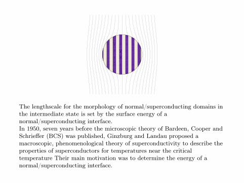
The lengthscale for the morphology of normal/superconducting domains inthe intermediate state is set by the surface energy of anormal/superconducting interface.In 1950, seven years before the microscopic theory of Bardeen, Cooper andSchrieffer (BCS) was published, Ginzburg and Landau proposed amacroscopic, phenomenological theory of superconductivity to describe theproperties of superconductors for temperatures near the criticaltemperature Their main motivation was to determine the energy of anormal/superconducting interface.

Maxwell’s equationsElectric field E, magnetic field H, current density J, and the charge density% satisfy

div E =%

ε, div H = 0, (1)

curl H = J, curl E + µ∂H

∂t= 0, (2)

where the permeability ε and the permittivity µ are assumed constant.When the wire is in the normal state we assume Ohm’s law

J = ςE, (3)

where ς is the constant electrical conductivity.Equation (1b) implies the existence of A such that

µH = curl A. (4)

Now equation (2b) implies

curl(E +

∂A

∂t

)= 0,

which implies that there exists Φ such that

E +∂A

∂t= −∇Φ; (5)

A is unique up to the addition of a gradient. Once A is given Φ is uniqueup to the addition of a function of t.

The Ginzburg-Landau TheorySteady state: E = 0.

Superconducting order parameterSuperconducting order parameter Ψ such that |Ψ|2 represents the numberdensity of superconducting electron pairs.However, Ψ is complex, and can be thought of as an ‘averaged macroscopicwavefunction’ for the superconducting electrons.

Ginzburg-Landau free energyWe proceed by expanding the Helmholtz free energy density F as a powerseries in |Ψ|2, which is truncated after the second term since |Ψ|2 is smallnear the critical temperature Tc. Thus, in the absence of a magnetic fieldwe have

Fs0 = Fn0 + a(T )|Ψ|2 +b(T )

2|Ψ|4.

In stable equilibrium we require

∂Fs0∂|Ψ|2 = 0,

∂2Fs0∂(|Ψ|2)2

> 0, with |Ψ|2 = 0 for T ≥ Tc,|Ψ|2 > 0 for T < Tc.

It follows that a(Tc) = 0, b(Tc) > 0, a(T ) < 0 for T < Tc. Thus, inequilibrium, for T < Tc,

|Ψ|2 = Ψ20 = −a

b.

T > Tc T < Tc

In a magnetic field

In a magnetic field we must add the magnetic field energy density 12µ|H|2,

and the energy associated with the possible appearance of a gradient in Ψin the presence of the field. This last energy is taken to be

const.|∇Ψ|2. (6)

This penalises variations of the order parameter Ψ and can be thought of asrepresenting the ‘surface energy’. On the other hand, the free energy shouldbe gauge invariant (in the sense that if A is replaced by A +∇ω then thephase of Ψ can be adjusted to make the resulting free energy densityindependent of ω), and we have yet to take into account the interactionbetween the magnetic field and the electric current associated with thepresence of a gradient in Ψ. Ginzburg and Landau therefore postulated theaddition of a term proportional to iAΨ to ∇Ψ, so that (6) becomes

1

2ms|i~∇Ψ + esAΨ|2 , (7)

where es = 2e and ms = 2m are the charge and mass respectively of thesuperconducting charge carriers, and 2π~ is Plank’s constant.

Note that (7) may be written

1

2ms

(~2|∇f |2 + |~∇χ− esA|2f2) ,

where Ψ = feiχ, with f and χ real, f > 0.The first term here is the surface energy term which penalises curvature inthe level sets of f .The second term may be interpreted as a gauge-invariant ‘kinetic energydensity’ associated with the superconducting currents.We will see later that the superconducting current is given by

Js = (esf2/ms)(~∇χ− esA).

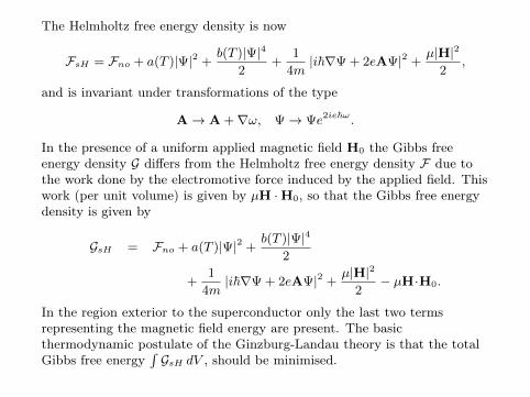
The Helmholtz free energy density is now

FsH = Fno + a(T )|Ψ|2 +b(T )|Ψ|4

2+

1

4m|i~∇Ψ + 2eAΨ|2 +

µ|H|2

2,

and is invariant under transformations of the type

A→ A +∇ω, Ψ→ Ψe2ie~ω.

In the presence of a uniform applied magnetic field H0 the Gibbs freeenergy density G differs from the Helmholtz free energy density F due tothe work done by the electromotive force induced by the applied field. Thiswork (per unit volume) is given by µH ·H0, so that the Gibbs free energydensity is given by

GsH = Fno + a(T )|Ψ|2 +b(T )|Ψ|4

2

+1

4m|i~∇Ψ + 2eAΨ|2 +

µ|H|2

2− µH·H0.

In the region exterior to the superconductor only the last two termsrepresenting the magnetic field energy are present. The basicthermodynamic postulate of the Ginzburg-Landau theory is that the totalGibbs free energy

∫GsH dV , should be minimised.

The critical field

In the normal state Ψ = 0, and∫GsH dV is minimised by H = H0, giving∫

GsH dV =

∫Fno −

1

2µH2

0 dV.

In the perfect superconducting state in the absence of surface effects∫GsH dV is minimised by H = 0, Ψ = −a/b, giving∫

GsH dV =

∫Fno −

a2

2bdV.

We see that for low values of H0 the superconducting state has a lower freeenergy, whereas for high values of H0 the normal state has a lower freeenergy. Thus there is a critical magnetic field at which, in the absence ofsurface effects (i.e. for a bulk superconductor), the superconducting statebecomes energetically more favourable. We see that this field is given by

Hc =|a(T )|õb(T )

. (8)

Steady state Ginzburg-Landau equations

If the superconductor occupies a region Ω ⊂ R3 the Euler-Lagrangeequations associated with the minimisation of the free energy with respectto Ψ∗ and A are the celebrated Ginzburg-Landau equations

1

4m(~∇− 2ieA)2 Ψ = a(T )Ψ + b(T )|Ψ|2Ψ in Ω, (9)

1

µ(curlA)2 = −

ie~2m

(Ψ∗∇Ψ−Ψ∇Ψ∗) +2e2

m|Ψ|2A in Ω, (10)

1

µ(curlA)2 = curl H0 outside Ω, (11)

with the natural boundary conditionsn · (~∇− 2ieA) Ψ = 0 on ∂Ω, (12)[(1/µ)curl A ∧ n] = 0, (13)

curl A → µH0 as r →∞, (14)

where [ ] denotes the jump in the enclosed quantity across ∂Ω and r is thedistance from the origin.

Two important lengthscales

We see that there are two important lengthscales associated with (9)-(10).From (9) we see that the natural lengthscale for variations in Ψ is

ξ =~

2√m|a|

,

which is known as the coherence length, while from (10) we see that thenatural lengthscale for variations in A (and therefore H) is

λ =1

e

√mb

2|a|µ,

which is known as the penetration depth. The penetration depth measuresthe depth that a small external magnetic field will penetrate into asuperconductor. The ratio of these two lengthscales is the nondimensionalGinzburg-Landau parameter κ = λ/ξ is a key material parameter indetermining the behaviour of the superconductor.

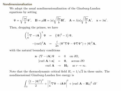
NondimensionalisationWe adopt the usual nondimensionalization of the Ginzburg-Landauequations by setting

Ψ =

√|a|b

Ψ′, B = µH = |a|√

2µ

bH′, A = λ|a|

√2µ

bA′, x = λx′.

Then, dropping the primes, we have(1

κ∇− iA

)2

Ψ =(|Ψ|2 − 1

)Ψ,

−(curl)2A =i

2κ(Ψ∗∇Ψ−Ψ∇Ψ∗) + |Ψ|2A,

with the natural boundary conditions

n · (∇− iA) Ψ = 0 on ∂Ω,

[curl A ∧ n] = 0, across ∂Ω

curl A → H0 as r →∞.

Note that the thermodynamic critical field Hc = 1/√

2 in these units. Thenondimensional Ginzburg-Landau free energy is∫

Ω

(1− |Ψ|2

)22

+

∣∣∣∣ 1κ∇Ψ− iAΨ

∣∣∣∣2 + |curl A−H0|2 dV

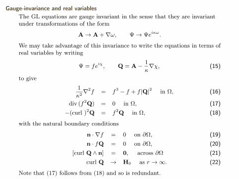
Gauge-invariance and real variablesThe GL equations are gauge invariant in the sense that they are invariantunder transformations of the form

A→ A +∇ω, Ψ→ Ψeiκω.

We may take advantage of this invariance to write the equations in terms ofreal variables by writing

Ψ = feiχ, Q = A− 1

κ∇χ, (15)

to give

1

κ2∇2f = f3 − f + f |Q|2 in Ω, (16)

div (f2Q) = 0 in Ω, (17)

−(curl )2Q = f2Q in Ω, (18)

with the natural boundary conditions

n · ∇f = 0 on ∂Ω, (19)

n · fQ = 0 on ∂Ω, (20)

[curl Q ∧ n] = 0, across ∂Ω (21)

curl Q → H0 as r →∞. (22)

Note that (17) follows from (18) and so is redundant.

Two dimensions

A commonly considered special case is the two-dimensional situation inwhich Ω is the cylinder D × R, D ⊆ R2, with an applied magnetic fieldH ≡ (0, 0, Hext) as x2 + y2 →∞. In this case the solutions are of the form

H = (0, 0, H(x, y, t)),

A = (A1(x, y, t), A2(x, y, t), 0),

and the Maxwell equations

curl H = 0, divH = 0,

outside Ω imply ∇H = 0, so that H ≡ Hext outside Ω1. Thus thecontinuity of magnetic field across ∂Ω leads to the Dirichlet conditionH = Hext on ∂D, and we do not have to consider the region external to thesuperconductor further. We note also that the potential A can be chosen sothat

A · n = 0 on ∂D.

We will return to this two-dimensional situation often throughout thecourse, since it is usually much simpler than the general case.

1If Ω is not simply connected then H ≡ Hext in the unbounded component of R3\Ω, butin each bounded component of R3\Ω (i.e. in the holes of Ω) all we can say is H =constant.These constants must be determined as part of the solution.

Normal-superconducting interfaceH = (0, 0, H(x)), A = (0, A(x), 0), H = dA/dx.dχ/dx = 0 ⇒ Ψ may be taken to be real. Then

1

κ2Ψ′′ = Ψ3 −Ψ +A2Ψ, (23)

A′′ = Ψ2A, (24)

where ′ ≡ d/dx. These equations form a Hamiltonian system, withHamiltonian given by

H =Ψ4

2−Ψ2 +A2Ψ2 − (Ψ′)2

κ2− (A′)2 = constant. (25)

For a normal/superconducting transition we have boundary conditions

A→ 0, Ψ→ 1, as x→ −∞, A′ → H0, Ψ→ 0, as x→∞,

where the field on the normal side of the region is equal to H0.The equations admit a solution if and only if H0 = Hc = 1/

√2.

To see this we note that the boundary conditions imply that the constant in(25) is −1/2.

Hence, in order for a normal/superconducting transition layer to exist thelimiting value of the field in the normal region as the domain boundary isapproached must be equal to Hc.

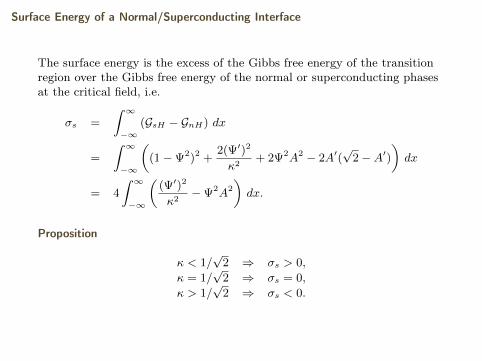
Surface Energy of a Normal/Superconducting Interface

The surface energy is the excess of the Gibbs free energy of the transitionregion over the Gibbs free energy of the normal or superconducting phasesat the critical field, i.e.

σs =

∫ ∞−∞

(GsH − GnH) dx

=

∫ ∞−∞

((1−Ψ2)2 +

2(Ψ′)2

κ2+ 2Ψ2A2 − 2A′(

√2−A′)

)dx

= 4

∫ ∞−∞

((Ψ′)2

κ2−Ψ2A2

)dx.

Proposition

κ < 1/√

2 ⇒ σs > 0,

κ = 1/√

2 ⇒ σs = 0,

κ > 1/√

2 ⇒ σs < 0.

Type I and Type II

DefinitionMaterials with κ < 1/

√2 are known as Type I superconductors.

Materials with κ > 1/√

2 are known as Type II superconductors.

Negative surface energies were dismissed at the time (1950) as beingphysically unrealistic. Abrikosov later investigated the nature of possiblesolutions in this case, and about 10 years after that Type IIsuperconductors were observed directly experimentally, and shown toexhibit the Abrikosov “mixed state”. It is one of the great achievements ofthe Ginzburg-Landau theory that it allowed for the possibility of Type IIsuperconductors before their existence had been verified.

The negative surface energy means a type-II superconductor wants tomaximise the area of the normal/superducting interface. This means it isbetter to make two small normal regions than one large one. The result is alot of very small normal regions. However, because of flux quantization thenormal regions cannot be arbitrarily small.

The importance of phase: fluxoid quantization

Hole

penetration depth

Superconductor

C

Equation (18) gives an expressionfor the superconducting current,

J = curl H = curl 2Q = −f2Q.

Let C be a closed curve lying in thematerial such that f = |Ψ| 6= 0everywhere on C, and let S be asurface bounded by C. Then

−∫C

1

|Ψ|2 J · ds =

∫C

Q · ds

=

∫C

A · ds− 1

κ

∫C

∇χ · ds =

∫S

H · n dS − 2πN

κ,

where N is an integer, since the phase χ must change by an integer multipleof 2π around C if Ψ is single valued. Hence∫

S

H · ndS +

∫C

1

|Ψ|2 J · ds =2πN

κ. (26)

The left-hand side of this equation is known as the fluxoid through thesurface S. If C is taken to be far enough inside the superconductor thatJ→ 0 and the second integral is negligible, then the magnetic flux throughS is quantized. Thus the magnetic flux through a hole is quantized if weinclude the flux that penetrates the superconductor.

Note that this result implies that the superconductor cannot formarbitrarily small normal regions, since such a region must contain at leastone quantum of flux.

Fluxoid quantization can also be used to explain the persistence of currentsin a ring of superconducting material (even though such a state has ahigher energy than that of no current). The current in such a ring cannotdecrease through fluctuations by arbitrarily small amounts, but only infinite jumps such that the fluxoid decreases by one or more integermultiples of 2π/κ. If only a single or a few electrons were involved, thiscould easily be accomplished. However, we are requiring a quantum jumpin the phase of Ψ, a macroscopic function. Such a change requires thesimultaneous quantum jump of a very large (> 1020) number of particles,and is of course extremely improbable, leading to an extremely long half lifefor circulating superconducting currents.

Type II superconductors

NORMAL

MIXED

SUPERCONDUCTING

Hc2(T )

Hc1(T )

TTc

Happ H

Hc2Hc1 Happ

S M N

As the external magnetic field is raised for a Type I superconductor there isa transition from superconducting to normal at H0 = Hc. For a Type IIsuperconductor, however, there is first a transition to a mixed state whenH0 reaches a lower critical value Hc1 . The mixed state does not becomefully normal until the field reaches the upper critical value Hc2 .

Phase diagram

κ

H0

Type-I Type-II

Mixed

Normal

Superconducting

Hc

Hc2

Hc1

1√2

Mixed state

0 2 4 6 8

0

2

4

6

8

Steady vortices

Single quantum rectilinear vortex solutionIn the mixed state the magnetic field penetrates a type-II superconductorin “flux tubes” known as superconducting vortices. We seek a solution ofthe form

Ψ = f(r)einθ, A = A(r)eθ,

on an infinite domain. Then

1

κ2

1

r

d

dr

(r

df

dr

)−(A− n

κr

)2

f = f3 − f, (27)

d

dr

(1

r

d

dr(rA)

)= f2

(A− n

κr

), (28)

f, A bounded as r → 0, f → 1, A→ 0 as r →∞. (29)

The supercurrent is given by

J = curl H = −f2(A− n

κr

)eθ, (30)

which shows the vortex nature of this solution. The axial magnetic fieldcarried by the vortex is ∫

R2

H · dS =2πn

κ. (31)

J

H

1

f

1κ

Asymptotic analysis for large κ

For large values of κ, f ≈ 1 except in a region of order κ−1 from the origin,which is the vortex core.

Leading-order outer regionAway from the origin we expand the outer solution, denoted by thesubscript o, as

f ≡ fo ∼ f (0)o +

1

κf (1)o + · · · ,

A ≡ Ao ∼ A(0)o +

1

κA(1)o + · · · .

At leading order we find

(f (0)o )2 = 1− (A(0)

o )2, (32)d

dr

(1

r

d

dr

(rA(0)

o

))= A(0)

o − (A(0)o )3, (33)

A(0)o bounded as r → 0, (34)

A(0)o → 0 as r →∞. (35)

Hence A(0)o ≡ 0, f (0)

o ≡ 1. Thus we find that away from the vortex core f isunity to leading order, and A and H are of order 1/κ.

Leading-order inner regionNear the origin we rescale lengths by setting r = R/κ, to obtain the innerequation, denoted by the subscript i, as

1

R

d

dR

(R

dfidR

)−(Ai −

n

R

)2

fi = f3i − fi, (36)

κ2 d

dR

(1

R

d

dR(RAi)

)= f2

i

(Ai −

n

R

). (37)

We expand the inner solution as

fi ∼ f(0)i +

1

κf

(1)i + · · · ,

Ai ∼ A(0)i +

1

κA

(1)i + · · · .

At leading order we find

1

R

d

dR

(R

df(0)i

dR

)−(A

(0)i −

n

R

)2

f(0)i = (f

(0)i )3 − f (0)

i , (38)

d

dR

(1

R

d

dR

(RA

(0)i

))= 0, (39)

f(0)i , A

(0)i bounded as R→ 0. (40)

Matching with the outer solution gives

f(0)i → 1, A

(0)i → 0 as R→∞.

Hence A(0)i ≡ 0, and

1

R

d

dR

(R

df(0)i

dR

)− n2

R2f

(0)i = (f

(0)i )3 − f (0)

i , (41)

f(0)i , bounded as R→ 0, (42)

f(0)i → 1, as R→∞. (43)

Not suprisingly, we will find that the leading order behaviour near thevortex core of more general vortex lines will also be given by (41)-(43). Theexistence of a unique solution to (41)-(43) has been proved by Chen et al..

First-order outer region

Equating coefficients of 1/κ in the outer equations (27)-(28) we find

0 = 3(f (0)o )2f (1)

o − f (1)o , (44)

d

dr

(1

r

d

dr(rA(1)

o )

)= (f (0)

o )2(A(1)o −

n

r

), (45)

or, using the fact that f (0)o ≡ 1,

f (1)o = 0, (46)

d

dr

(1

r

d

dr(rA(1)

o )

)=

(A(1)o −

n

r

), (47)

Matching with the inner region requires A(1)o = o(1/r) as r → 0. The

solution to (47) which decays at infinity is

A(1)o =

n

r− nK1(r), (48)

where K1 is the modified Bessel function.The magnetic field

H(1)o =

1

r

d

dr(rA(1)

o ) = nK0(r).

Second-order outer region

Equating coefficients of 1/κ2 in the outer equations (27) we find

f (2)o = −1

2

(A(1)o −

n

r

)2

= −1

2n2K1(r)2. (49)

Summary

Outer expansion

fo ∼ 1− 1

2κ2n2K1(r)2 + · · · ,

Ao =1

κ

(nr− nK1(r)

)+ · · · ,

Ho =n

κK0(r) + · · · .

Inner expansion

fi = f(0)i (R) + · · · ,

Ai =1

κ2A

(2)i (R) + + · · · .

Energy of a vortex

The energy of the vortex minus the energy of the pure superconductingstate is

E = 2π

∫ ∞0

((1− f2)2

2+

(df

dr

)2

+ f2(A−

n

κr

)2+ (H −Hext)2 −H2

ext

)r dr

= π

∫ ∞0

(1− f4 + 2(H2 − 2HHext)

)r dr,

We can use the asymptotic expansion of the previous section toapproximate the energy for large κ. Consider, for 1/κ δ 1,∫ ∞

0

(1− f4) r dr =

∫ δ

0

(1− f4)rdr +

∫ ∞δ

(1− f4)r dr

=1

κ2

∫ δκ

0

(1− f4i )RdR+

∫ ∞δ

(1− f4o )r dr

∼ 1

κ2

∫ δκ

0

(1− (f(0)i )4)RdR− 4

κ2

∫ ∞δ

f (2)o r dr

=1

κ2

∫ δκ

0

(1− (f(0)i )4)RdR+

2

κ2

∫ ∞δ

n2K1(r)2r dr

∼ 1

κ2

∫ δκ

0

(1− (f(0)i )4)RdR+

2n2

κ2(log 2/δ − 1/2− γ).

Energy of a vortex

(f(0)i )2 ∼ 1− n2

R2as R→∞ ⇒ 1− (f

(0)i )4 ∼ 2n2

R2as R→∞

and the upper limit of the first integral also gives a logarithmic singularity.We write∫ δκ

0

(1− (f(0)i )4)RdR =

∫ 1

0

(1− (f(0)i )4)RdR+

∫ δκ

1

(1− (f(0)i )4)RdR

=

∫ 1

0

(1− (f(0)i )4)RdR+

∫ δκ

1

(1− (f

(0)i )4 − 2n2

R2

)RdR+

∫ δκ

1

2n2

RdR

∼∫ 1

0

(1− (f(0)i )4)RdR+

∫ ∞1

(1− (f

(0)i )4 − 2n2

R2

)RdR+ 2n2 log(δκ).

Thus ∫ ∞0

(1− f4) r dr ∼ 2n2 log κ

κ2+C

κ2

where

C =

∫ 1

0

(1−(f(0)i )4)RdR+

∫ ∞1

(1− (f

(0)i )4 − 2n2

R2

)RdR+2n2(log 2−1/2−γ).

Energy of a vortex

Now ∫ ∞0

2(H2 − 2HHext)r dr =1

κ2− 4Hext

κ.

Thus

E =2n2 log κ

κ2+C

κ2+

1

κ2− 4Hext

κ.

We see that the energy of an index 2 vortex is twice that of two index 1vortices. Thus only vortices with indices ±1 are expected to be stable.The critical field, at which it becomes energetically favourable to have avortex, is

Hc1 =log κ

2κ+C

4κ+

1

4κ.