arX

iv:n

lin/0

6060

70v1

[nl

in.S

I] 2

8 Ju

n 20

06

Journal of Physics A. Vol.39. No.26. (2006) pp.8395-8407.

Psi-Series Solution of Fractional Ginzburg-LandauEquation

Vasily E. Tarasov

Skobeltsyn Institute of Nuclear Physics,

Moscow State University, Moscow 119992, Russia

E-mail: tarasov@theory.sinp.msu.ru

Abstract

One-dimensional Ginzburg-Landau equations with derivatives of noninteger or-

der are considered. Using psi-series with fractional powers, the solution of the frac-

tional Ginzburg-Landau (FGL) equation is derived. The leading-order behaviours of

solutions about an arbitrary singularity, as well as their resonance structures, have

been obtained. It was proved that fractional equations of order α with polynomial

nonlinearity of order s have the noninteger power-like behavior of order α/(1 − s)

near the singularity.

PACS numbers: 05.45.-a; 45.10.Hj

1 Introduction

Differential equations that contain derivatives of noninteger order [1, 2] are called frac-

tional equations [3, 4]. The interest to fractional equations has been growing continually

during the last few years because of numerous applications. In a fairly short period of

time the areas of applications of fractional calculus have become broad. For example, the

derivatives and integrals of fractional order are used in chaotic dynamics [5, 6], material

sciences [7, 8, 9], mechanics of fractal and complex media [10, 11], quantum mechan-

ics [12, 13], physical kinetics [5, 14, 15, 16], plasma physics [17, 18], astrophysics [19],

long-range dissipation [20], non-Hamiltonian mechanics [21, 22], long-range interaction

[23, 24, 25], anomalous diffusion and transport theory [5, 26, 27].

1

The fractional generalization of the Ginzburg-Landau equation was suggested in [28].

This equation can be used to describe the dynamical processes in continuums with fractal

dispersion and the media with fractal mass dimension [29, 30, 31]. In this paper, we

generalize the psi-series approach to the fractional differential equations. As an example,

we consider a solution of the fractional Ginzburg-Landau (FGL) equation. We derive

the psi-series for the one-dimensional FGL equation. The leading-order behaviours of

solutions about an arbitrary singularity, as well as their resonance structures, have been

obtained.

In section 2, we recall the appearance of the Ginzburg-Landau equation with fractional

derivatives. In section 3, the singular behavior of the FGL equation is considered. In

section 4, we discuss the powers of series terms that have arbitrary coefficients that are

called the resonances or Kovalevskaya exponents. In section 5, we derive the psi-series and

recurrence relations for one-dimensional FGL equation with rational order α (1 < α < 2).

In section 6, the example of an FGL equation with order α = 3/2 is suggested. In section

7, the next to singular behaviour for arbitrary (rational or irrational) order is discussed.

Finally, a short conclusion is given in section 8.

2 Fractional Ginzburg-Landau (FGL) equation

Let us recall the appearance of the nonlinear parabolic equation [32, 33, 34, 35], and the

FGL equation [28, 29, 31]. Consider wave propagation in some media and present the

wave vector k in the form

k = k0 + κ = k0 + κ‖ + κ⊥, (1)

where k0 is the unperturbed wave vector and subscripts (‖,⊥) are taken respectively to

the direction of k0. A symmetric dispersion law ω = ω(k) for κ≪ k0 can be written as

ω(k) = ω(|k|) ≈ ω(k0) + vg (|k| − k0) +1

2v′

g (|k| − k0)2, (2)

where

vg =

(

∂ω

∂k

)

k=k0

, v′g =

(

∂2ω

∂k2

)

k=k0

, (3)

and

|k| = |k0 + κ| =√

(k0 + κ‖)2 + κ2⊥ ≈ k0 + κ‖ +

1

2k0κ2⊥. (4)

2

Substitution of (4) into (2) gives

ω(k) ≈ ω0 + vgκ‖ +vg

2k0

κ2⊥ +

v′g

2κ2‖, (5)

where ω0 = ω(k0). Expression (5) in the dual space (”momentum representation”) corre-

sponds to the following equation in the coordinate space:

i∂Z

∂t= ω0Z − ivg

∂Z

∂x− vg

2k0∆⊥Z −

v′g

2∆‖Z (6)

with respect to the field Z = Z(t, x, y, z), where x is along k0, and we use the operator

correspondence between the dual space and usual space-time:

ω(k) ←→ i∂

∂t, κ‖ ←→ −i

∂

∂x,

(κ⊥)2 ←→ −∆⊥ = − ∂2

∂y2− ∂2

∂z2, (κ‖)

2 ←→ −∆‖ = − ∂2

∂x2. (7)

A generalization to the nonlinear case can be carried out similarly to (5) through a

nonlinear dispersion law dependence on the wave amplitude:

ω = ω(k, |Z|2) ≈ ω(k, 0) + b|Z|2 = ω(|k|) + b|Z|2 (8)

with some constant b = ∂ω(k, |Z|2)/∂|Z|2 at |Z| = 0. In analogy to (6), we obtain from

(5) and (7):

i∂Z

∂t= ω(k0)Z − ivg

∂Z

∂x− vg

2k0∆⊥Z −

v′g

2∆‖Z + b|Z|2Z. (9)

This equation is known as the nonlinear parabolic equation [32, 33, 34, 35]. The change

of variables from (t, x, y, z) to (t, x− vgt, y, z) gives

−i∂Z

∂t=

vg

2k0

∆⊥Z +v′

g

2∆‖Z − ω(k0)Z − b|Z|2Z (10)

that is also known as the nonlinear Schrodinger (NLS) equation.

Wave propagation in media with fractal properties can be easily generalized by rewrit-

ing the dispersion law (5), (8) in the following way [28]:

ω(k, |Z|2) = ω(k0, 0) + vgκ‖ + g1(κ2⊥)α/2 + g2(κ

2‖)

β/2 + b|Z|2, (1 < α, β < 2) (11)

3

with new constants g1, g2.

Using the connection between Riesz fractional derivative and its Fourier transform [1]

(−∆⊥)α/2 ←→ (κ2⊥)α/2, (−∆‖)

β/2 ←→ (κ2‖)

β/2, (12)

we obtain from (11)

i∂Z

∂t= −ivg

∂Z

∂x+ g1(−∆⊥)α/2Z + g2(−∆‖)

β/2Z + ω0Z + b|Z|2Z, (13)

where Z = Z(t, x, y, z). By changing the variables from (t, x, y, z) to (t, ξ, y, z), ξ = x−vgt,

and using

(−∆‖)β/2 =

∂β

∂|x|β =∂β

∂|ξ|β , (14)

we obtain from (13) equation

i∂Z

∂t= g1(−∆⊥)α/2Z + g2(−∆‖)

β/2Z + ω0Z + b|Z|2Z, (15)

that can be called the fractional nonlinear parabolic equation. For g2 = 0 we get the

nonstationary FGL equation (fractional NLS equation) suggested in [28]. Let us comment

on the physical structure of (15). The first term on the right-hand side is related to wave

propagation in media with fractal properties. The fractional derivative can also appear

as a result of long-range interaction [23, 24, 25]. Other terms on the right-hand-side of

equations (13) and (15) correspond to wave interaction due to the nonlinear properties of

the media. Thus, equation (15) can describe fractal processes of self-focusing and related

issues.

We may consider one-dimensional simplifications of (15), i.e.,

i∂Z

∂t= g2

∂βZ

∂|ξ|β + ω0Z + b|Z|2Z, (16)

where Z = Z(t, ξ), ξ = x− vgt, or the equation

i∂Z

∂t= g1

∂αZ

∂|z|α + ω0Z + b|Z|2Z, (17)

where Z = Z(t, z). We can reduce (17) to the case of a propagating wave

Z = Z(z − vgt) ≡ Z(η). (18)

4

For the real field Z, Eq. (17) becomes

g1dαZ

d|η|α + cdZ

dη+ ω0Z + bZ3 = 0, η = z − vgt, (19)

where c = ivg. This equation takes the form of the fractional generalization of the

Ginzburg-Landau equation, when vg = 0.

It is well known that the nonlinear term in equations of type (10) leads to a steepening

of the solution and its singularity. The steepening process may be stopped by a diffusional

or dispersional term, i.e. by a higher derivative term. A similar phenomenon may appear

for the fractional nonlinear equations (19).

3 Singular behavior of FGL equation

There is an approach to the question of integrability which is not concerned with the

display of explicit functions, but with the demonstration of a specific property. This is

the existence of Laurent series for each of the dependent variables. The series may not

be summable to an explicit form, but does represent an analytic function. The essential

feature of this Laurent series is that it is an expansion about a particular type of movable

singularity, i.e., a pole. Consequently the existence of these Laurent series is intimately

concerned with the singularity analysis of differential equations initiated about a century

ago by Painleve, Gambier and Garnier [36] and continued since by many workers including

Bureau [37] and Cosgrove et al [38].

The connection of this type of singular behavior and the solution of partial differential

equations by the method of the inverse scattering transform was noticed by Ablowitz et al

[39] who developed an algorithm, called the ARS algorithm, to test whether the solution

of an ordinary differential equation was expressible in terms of a Laurent expansion. If

this was the case, the ordinary differential equation was said to pass the Painleve test and

was conjectured to be integrable. Under more precise conditions Conte [40] has shown

that the equation is integrable. Psi-series solutions of differential equations are considered

in [41, 42, 43, 44].

In the paper, we consider the fractional equation

gDαxZ(x) + cD1

xZ(x) + aZ(x) + bZ3(x) = 0, (20)

where 1 < α < 2, and Dαx is the fractional Riemann-Liouville derivative:

DαxZ(x) =

1

Γ(m− α)

dm

dxm

∫ x

x0

dyZ(y)

(x− y)α−m+1. (21)

5

Here, m is the first whole number greater than or equal to α. In our case m = 2. We

detect possible singular behavior in the solution of a differential equation by means of the

leading-order analysis.

To determine the leading-order behavior, we set

Z(x) = f(x− x0)p, (22)

where x0 is an arbitrary constant (the location of the singularity). Then, we substitute

(22) into the fractional differential equation (20) and look for two or more dominant

terms. The detection of which terms are dominant is identical to the determination of

which terms in an equation are self-similar.

Substituting (22) into equation (20), and using the relation

Dαxxp =

Γ(p + 1)

Γ(p + 1− α)xp−α, (p > −1), (23)

we get

gfΓ(p + 1)

Γ(p + 1− α)(x− x0)

p−α + cpf(x− x0)p−1 + af(x− x0)

p + bf 3(x− x0)3p = 0. (24)

If 1 < α < 2, then p− α < p− 1. For the dominant terms,

gfΓ(p + 1)

Γ(p + 1− α)(x− x0)

p−α + bf 3(x− x0)3p = 0. (25)

As a result, we obtain

p− α = 3p, (26)

gΓ(p + 1)

Γ(p + 1− α)+ bf 2 = 0. (27)

Equation (26) gives

p = −α

2. (28)

If 1 < α < 2, then −1 < p < −1/2. Therefore the leading-order singular behavior is

found:

Z(x) = f(x− x0)−α/2, f 2 +

gΓ(1− α/2)

bΓ(1− 3α/2)= 0, (29)

and the singularity is a pole of order α/2. Evidently our psi-series starts at (x− x0)−α/2.

The resonance conditions and psi-series is considered in the next sections.

As a result, we get that fractional differential equations of order α with polynomial

nonlinearity of order s have the noninteger power behavior of order α/(1 − s) near the

singularity.

6

4 Resonance terms of FGL equation

The powers of (x − x0) that have arbitrary coefficients are called the resonances or Ko-

valevskaya’s exponents. To find resonance, we consider the substitution

Z(x) = f(x− x0)p + l(x− x0)

p+r, (30)

and find the values r. In equation (30) parameters p and f are defined by

p = −α

2, f =

√

− gΓ(1− α/2)

bΓ(1− 3α/2). (31)

Substitution of Eq. (30) into (20) gives

gfΓ(p + 1)

Γ(p + 1− α)(x− x0)

p−α + cpf(x− x0)p−1 + af(x− x0)

p + bf 3(x− x0)3p+

+glΓ(p + r + 1)

Γ(p + r + 1− α)(x− x0)

p+r−α + cpl(x− x0)p+r−1 + al(x− x0)

p+r + bl3(x− x0)3p+3r+

+3bl2f(x− x0)2p+3r + 3blf 2(x− x0)

p+3r = 0. (32)

Using equation (31), and considering the linear with respect to l terms of (32), we have

Γ(1 + r − α/2)

Γ(1 + r − 3α/2)− 3

Γ(1− α/2)

Γ(1− 3α/2)= 0. (33)

This relation allows us to derive the values of r. Equation (33) can be directly derived

by using the recurrence relations. In the general case, the values of r can be irrational or

complex numbers. The solution of the FGL equation with 1 < α ≤ 2 have two arbitrary

parameters. Therefore, we must have two values of r that are the solutions of equation

(33). It is interesting to note that (33) gives two real values of r only for

α > α0, (34)

where

α0 ≈ 1.3005888986. (35)

The order α0 is an universal value that does not depends on values of parameters g, a, b,

c of the FGL equation (20).

7

The plots of the function

y(r) =Γ(1 + r − α/2)

Γ(1 + r − 3α/2)− 3

Γ(1− α/2)

Γ(1− 3α/2)(36)

are shown in figures 1 and 2. The solutions of equation (33) correspond to the points of

intersections with the horizontal axis.

As a result, the nature of the resonances is summarized as follows:

1) For α such that 1 < α < α0 the values of r are complex or r < −α/2.

2) For α such that α0 < α < 2, we have two the real values of r. Note that for α0 < α <

1.9999999995, the values r satisfy the inequality r < 6.426.

0,5

0,4

0,3

0,2

0,1

r

10,80,60,40,20

Figure 1: Plot for the order α = 1.30.

5 Psi-Series for FGL Equation of Rational Order

Let us consider the psi-series and recurrence relations for the one-dimensional FGL equa-

tion (20), where the order α is a rational number such that:

α =m

n, (1 < α < 2). (37)

Following a standard procedure [41], we substitute

Z(x) =1

(x− x0)α/2

∞∑

k=0

ekφk(x− x0), (38)

8

0,2

0,1

0,3

0

r

10,80,60,40,20

0,5

0,4

Figure 2: Plot for the order α = 1.31.

where

e0 = f =

√

− gΓ(1− α/2)

bΓ(1− 3α/2), (39)

into the fractional Ginzburg-Landau equation (20). Note that the coefficient e0 is a real

number for two cases: (1) g/b ≥ 0 and 1 < α < 4/3; (2) g/b ≤ 0 and 4/3 < α < 2.

For the rational order α = m/n, we suggest to use the φ-function in the form

φ(x− x0) = (x− x0)1/2n. (40)

Then

Z(x) =1

(x− x0)α/2

∞∑

k=0

ek(x− x0)βk =

∞∑

k=0

ek(x− x0)βk−α/2, (41)

where

βk =k

2n. (42)

In this case, the action of fractional derivative of order α = m/n can be represented as

the change of the number of term ek → ek−2m:

Dαx (x− x0)

βk =Γ(βk + 1)

Γ(βk−2m + 1)(x− x0)

βk−2m . (43)

9

It allows us to derive the generalized psi-series solutions of fractional Ginzburg-Landau

equation.

Substitution of the series

Z(x) =∞∑

k=0

ek(x− x0)βk−α/2 =

∞∑

k=0

ek(x− x0)k−m2n (44)

into equation (20) gives

g

∞∑

k=0

ek

Γ(k−m+2n2n

)

Γ(k−3m+2n2n

)(x− x0)

k−3m2n + c

∞∑

k=0

ekk −m

2n(x− x0)

k−m−2n2n +

+a∞∑

k=0

ek(x− x0)k−m2n + b

∞∑

k1=0

∞∑

k2=0

∞∑

k3=0

ek1ek2

ek3(x− x0)

k1+k2+k3−3m2n = 0. (45)

Let us compute ek (k = 1, 2, ...) through the equation of coefficients of like power of

(x− x0) to zero in (45):

g∞∑

k=0

ek

Γ(k−m+2n2n

)

Γ(k−3m+2n2n

)(x− x0)

k−3m2n + c

∞∑

k=2m−2n

ek−2m+2nk − 3m + 2n

2n(x− x0)

k−3m2n +

+a

∞∑

k=2m

ek−2m(x− x0)k−3m

2n + 3be20

∞∑

k=0

ek(x− x0)k−3m

2n +

+b∞∑

k=0

k−1∑

i=1

i∑

j=1

ek−i−jeiej(x− x0)k−3m

2n = 0. (46)

Using e20 = f 2, we get

gek

Γ(k−m+2n2n

)

Γ(k−3m+2n2n

)+ cek−2m+2n

k − 3m + 2n

2n+

+aek−2m + 3bf 2ek + b

k−1∑

i=1

i∑

j=1

ek−i−jeiej = 0. (47)

Here k = 0, 1, 2, ..., and ek = 0 for k < 0. We can rewrite the recurrence relation (47) as

ek

(

gΓ(k−m+2n

2n)

Γ(k−3m+2n2n

)+ 3bf 2

)

= −cek−2m+2nk − 3m + 2n

2n− aek−2m − b

k−1∑

i=1

i∑

j=1

ek−i−jeiej,

(48)

10

where

f 2 = − gΓ(1− α/2)

bΓ(1− 3α/2)= − gΓ(2n−m

2n)

bΓ(2n−3m2n

). (49)

Substitution of equation (49) into equation (48) gives

ekg

(

Γ(k−m+2n2n

)

Γ(k−3m+2n2n

)− 3Γ(2n−m

2n)

Γ(2n−3m2n

)

)

= −cek−2m+2nk − 3m + 2n

2n− aek−2m−

−bk−1∑

i=1

i∑

j=1

ek−i−jeiej . (50)

Note that we get resonances for the k that satisfies the condition

Γ(k−m+2n2n

)

Γ(k−3m+2n2n

)− 3Γ(2n−m

2n)

Γ(2n−3m2n

)= 0. (51)

In this case, the coefficient ek can be arbitrary.

As a result, we obtain the nonresonance terms

ek = −A(k, m, n)

(

cek−2m+2nk − 3m + 2n

2n+ aek−2m + b

k−1∑

i=1

i∑

j=1

ek−i−jeiej

)

, (52)

where

A(k, m, n) = − Γ(k−3m+2n2n

)Γ(2n−3m2n

)

g[Γ(k−m+2n2n

)Γ(2n−3m2n

)− 3Γ(k−3m+2n2n

)Γ(2n−m2n

)]. (53)

6 Fractional Ginzburg-Landau Equation with α = 1.5

Let us consider the FGL equation (20) with derivative of order α = 3/2. In this case,

n = 2, m = 3, and the coefficients ek are defined by

ek = −

(

cek−2k−54

+ aek−6 + b∑k−1

i=1

∑ij=1 ek−i−jeiej

)

Γ(k−54

)Γ(−54

)

g[Γ(k+14

)Γ(−54

)− 3Γ(k−54

)Γ(14)]

. (54)

For k = 0, we have

e0 = f =

√

− gΓ(14)

bΓ(−54

), (55)

where Γ(14)/Γ(−5

4) > 0, and we suppose g/b < 0. For k = 1, equation (54) leads to e1 = 0.

For k = 2,

e2 =3ce0Γ(−3

4)Γ(−5

4)

4g[Γ(34)Γ(−5

4)− 3Γ(−3

4)Γ(1

4)]

. (56)

11

Using the relation (55), we get

e2 = −c√

−5(g/b)π3/223/4Γ(3/4)

2g[2Γ4(3/4) + 5π2]. (57)

For k = 3, e3 = 0. For k = 4,

e4 = −(

ce2−14

+ be0e22

)

Γ(−14

)Γ(−54

)

g[Γ(54)Γ(−5

4)− 3Γ(−1

4)Γ(1

4)]

. (58)

Substitution of (55), and (57) into (58) gives

e4 =c2

√

5gπ√

2/bΓ7(3/4)

4g2[2Γ4(3/4) + 5π2]2(59)

For k = 5, we have e5 = 0. For k = 6, equation (54) is

e6 = −(

ce414

+ ae0 + be32 + 2be0e2e4

)

Γ(14)Γ(−5

4)

g[Γ(74)Γ(−5

4)− 3Γ(1

4)Γ(1

4)]

. (60)

Substituting e0, e2 and e4 from equations (55), (57), and (59) into (60), we have

e6 = −√

−5g/bπ3/223/4Γ(3/4)

3g2[2Γ4(3/4) + 5π2]3[2Γ4(3/4)− 5π2]

(

c3Γ12(3/4) + 5c3Γ8(3/4)π2+

+20c3Γ4(3/4)π4+16ag2Γ12(3/4)+120ag2Γ8(3/4)π2+300ag2Γ4(3/4)π4+250ag2π6)

. (61)

As the result, we obtain

Z(x) =∞∑

k=0

ek(x− x0)k−3

4 =

= e0(x− x0)−3/4 + e2(x− x0)

−1/4 + e4(x− x0)1/4 + e6(x− x0)

3/4 + ... (62)

This is a power psi-series that present the solution of FGL equation of order α = 1.5.

The coefficients in equation (62) are defined by equations (55), (57), (59), and (61). For

example, a = −b = c = g = 1 gives

e0 ≈ 0.9615539375, e2 ≈ −0.2382246293,

e4 ≈ 0.001685563496, e6 ≈ 0.3872134448.

12

7 Next to Singular Behavior

In sections 5 and 6, we consider the rational α. In this section, we suppose that the order

α is an arbitrary (rational or irrational). Instead of imposing a series commencing at the

power indicated by the singularity found by the leading-order analysis, we can determine

the next to singular behavior by writing

Z(x) = f(x− x0)p + G(x), (63)

where

p = −α

2, f =

√

− gΓ(1− α/2)

bΓ(1− 3α/2). (64)

We can always write Z(x) in the form (63). To make the process useful, we require that

the first term be the leading order term, i.e.,

(x− x0)−pG(x) = (x− x0)

α/2G(x)→ 0 if (x− x0)→ 0. (65)

Substituting (63) into (20), and using (23), we have

gfΓ(p + 1)

Γ(p + 1− α)(x− x0)

p−α + cpf(x− x0)p−1 + af(x− x0)

p + bf 3(x− x0)3p+

+gDαxG(x)+cD1

xG(x)+aG(x)+bG3(x)+3bf 2(x−x0)2pG(x)+3bf(x−x0)

pG2(x) = 0. (66)

Equations (66) and (64) give

gDαxG(x) + cD1

xG(x) + aG(x) + bG3(x) + 3bf 2(x− x0)2pG(x)+

+3bf(x− x0)pG2(x)cpf(x− x0)

p−1 + af(x− x0)p = 0. (67)

Multiplying this equation on (x − x0)−3p, and using condition (65), we get the equation

without nonlinear terms for (x− x0)→ 0.

As the result, we obtain

gDαxG(x) + cD1

xG(x) + aG(x) + cpf(x− x0)−α/2−1 + af(x− x0)

−α/2 = 0, (68)

with condition (65) for the solutions. Equation (68) is a linear inhomogeneous frac-

tional equation. The solution of this equation allows us to find the solution of the one-

dimensional FGL equation.

13

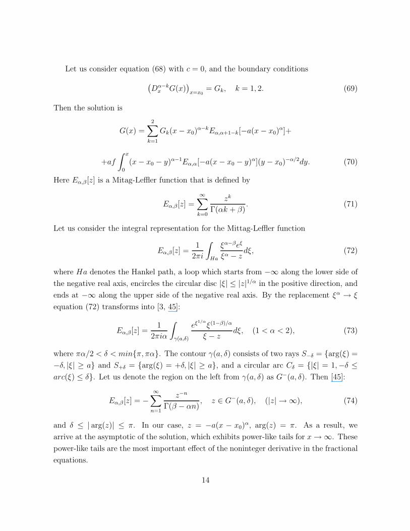
Let us consider equation (68) with c = 0, and the boundary conditions

(

Dα−kx G(x)

)

x=x0= Gk, k = 1, 2. (69)

Then the solution is

G(x) =

2∑

k=1

Gk(x− x0)α−kEα,α+1−k[−a(x− x0)

α]+

+af

∫ x

0

(x− x0 − y)α−1Eα,α[−a(x− x0 − y)α](y − x0)−α/2dy. (70)

Here Eα,β [z] is a Mitag-Leffler function that is defined by

Eα,β[z] =

∞∑

k=0

zk

Γ(αk + β). (71)

Let us consider the integral representation for the Mittag-Leffler function

Eα,β [z] =1

2πi

∫

Ha

ξα−βeξ

ξα − zdξ, (72)

where Ha denotes the Hankel path, a loop which starts from −∞ along the lower side of

the negative real axis, encircles the circular disc |ξ| ≤ |z|1/α in the positive direction, and

ends at −∞ along the upper side of the negative real axis. By the replacement ξα → ξ

equation (72) transforms into [3, 45]:

Eα,β[z] =1

2πiα

∫

γ(a,δ)

eξ1/αξ(1−β)/α

ξ − zdξ, (1 < α < 2), (73)

where πα/2 < δ < min{π, πα}. The contour γ(a, δ) consists of two rays S−δ = {arg(ξ) =

−δ, |ξ| ≥ a} and S+δ = {arg(ξ) = +δ, |ξ| ≥ a}, and a circular arc Cδ = {|ξ| = 1,−δ ≤arc(ξ) ≤ δ}. Let us denote the region on the left from γ(a, δ) as G−(a, δ). Then [45]:

Eα,β [z] = −∞∑

n=1

z−n

Γ(β − αn), z ∈ G−(a, δ), (|z| → ∞), (74)

and δ ≤ | arg(z)| ≤ π. In our case, z = −a(x − x0)α, arg(z) = π. As a result, we

arrive at the asymptotic of the solution, which exhibits power-like tails for x→∞. These

power-like tails are the most important effect of the noninteger derivative in the fractional

equations.

14

8 Conclusion

In this paper, we generalize the psi-series approach to the fractional differential equations.

As an example, we consider the fractional Ginzburg-Landau (FGL) equation [28, 29, 30,

31]. The suggested psi-series approach can be used for a wide class of fractional nonlinear

equations. The leading-order behaviours of solutions about an arbitrary singularity, as

well as their resonance structures, can be derived for fractional equations by the suggested

generalization of psi-series.

In the paper, we use the series

Z(x) =1

(x− x0)m/2n

∞∑

k=0

ek (x− x0)k/2n, (75)

where k, m, n are the integer numbers. For the order α = m/n, the action of fractional

derivative

Dαx (x− x0)

k/2n =Γ(k/2n + 1)

Γ((k − 2m)/2n + 1)(x− x0)

(k−2m)/2n (76)

can be represented as the change of the number of term ek → ek−2m in (75). It allows us

to derive the psi-series for the fractional differential equation of order α = m/n. For the

FGL equation the leading-order singular behaviour is defined by power that is equal to

the half of derivative order.

A remarkable property of the dynamics described by the equation with fractional space

derivatives is that the solutions have power-like tails [25]. In this paper, we prove that

fractional differential equations of order α with a polynomial nonlinear term of order s

have the noninteger power-like behavior of order α/(1− s) near the singularity.

It is interesting to find barriers to integrability for fractional differential equations. In

general, the integrability of fractional nonlinear equations is a very interesting object for

future researches. It has many problems that are connected with specific properties of

the fractional calculus. For example, we must derive a generalization of the Lie algebra

for the vector fields that are defined by fractional derivatives. For this generalization, the

Jacobi identity cannot be satisfied, and we have a non-Lie algebra. The definition of such

”fractional” Lie algebra is an open question and cannot be realized by a simple way. To

formulate the fractional generalization of a Lie algebra for derivatives of noninteger oder,

we can use the representation of fractional derivatives as infinite series of derivatives

of integer orders [1]. For example, the Riemann-Liouville fractional derivative can be

15

represented as

Dαx =

∞∑

n=0

An(x, x0, α)dn

dxn, (77)

where

An(x, a, α) =(−1)n−1αΓ(n− α)

Γ(1− α)Γ(n + 1)

(x− x0)n−α

Γ(n + 1− α). (78)

Then the possible realization of the generalization is connected with the special algebraic

structures for infinite jets [46]. These structures and approaches can help to solve some

problems that are connected with the integrability of fractional nonlinear equations.

References[1] S.G. Samko, A.A. Kilbas, O.I. Marichev, Fractional Integrals and Derivatives Theory and

Applications (Gordon and Breach, New York, 1993)

[2] K.B. Oldham, J. Spanier, The Fractional Calculus (Academic Press, New York, 1974)

[3] I. Podlubny, Fractional Differential Equations (Academic Press, New York, 1999)

[4] A.A. Kilbas, H.M. Srivastava, J.J. Trujillo, Theory and Applications of Fractional Differ-

ential Equations (Elsevier, Amsterdam, 2006)

[5] G.M. Zaslavsky, ”Chaos, fractional kinetics, and anomalous transport” Phys. Rep. 371

(2002) 461-580.

[6] G.M. Zaslavsky, Hamiltonian Chaos and Fractional Dynamics (Oxford University Press,

Oxford, 2005)

[7] Applications of Fractional Calculus in Physics Ed. by R. Hilfer (World Scientific, Singapore,

2000)

[8] M. Caputo, Elasticita e Dissipazione (Zanichelli, Bologna, 1969)

[9] R.R. Nigmatullin, ”The realization of the generalized transfer equation in a medium with

fractal geometry” Phys. Status Solidi B 133 (1986) 425-430; ”Fractional integral and its

physical interpretation” Theor. Math. Phys. 90 (1992) 242-251.

[10] A. Carpinteri, F. Mainardi, Fractals and Fractional Calculus in Continuum Mechanics

(Springer, New York, 1997)

[11] V.E. Tarasov, ”Continuous medium model for fractal media” Phys. Lett. A 336 (2005)

167-174 (cond-mat/0506137); ”Fractional hydrodynamic equations for fractal media” Ann.

Phys. 318 (2005) 286-307 (physics/0602096); ”Fractional Fokker-Planck equation for frac-

tal media” Chaos 15 (2005) 023102 (nlin.CD/0602029); ”Wave equation for fractal solid

string” Mod. Phys. Lett. B 19 (2005) 721-728 (physics/0605006); ”Possible experimental

test of continuous medium model for fractal media” Phys. Lett. A 341 (2005) 467-472

(physics/0602121).

16

[12] N. Laskin, ”Fractals and quantum mechanics” Chaos 10 (2000) 780-790; ”Fractional quan-

tum mechanics” Phys. Rev. E 62 (2000) 3135-3145; ”Fractional quantum mechanics and

Levy path integrals” Phys. Lett. A 268 (2000) 298-305 (hep-ph/9910419); ”Fractional

Schrodinger equation” Phys. Rev. E 66 (2002) 056108 (quant-ph/0206098).

[13] M. Naber, ”Time fractional Schrodinger equation” J. Math. Phys. 45 (2004) 3339-3352

(math-ph/0410028).

[14] G.M. Zaslavsky, ”Fractional kinetic equation for Hamiltonian chaos” Physica D 76 (1994)

110-122.

[15] A.I. Saichev, G.M. Zaslavsky, ”Fractional kinetic equations: solutions and applications”

Chaos 7 (1997) 753-764.

[16] G.M. Zaslavsky, M.A. Edelman, ”Fractional kinetics: from pseudochaotic dynamics to

Maxwell’s demon” Physica D 193 (2004) 128-147.

[17] B.A. Carreras, V.E. Lynch, G.M. Zaslavsky, ”Anomalous diffusion and exit time distribu-

tion of particle tracers in plasma turbulence model” Physics of Plasmas 8 (2001) 5096-5103.

[18] V.E. Tarasov, ”Electromagnetic field of fractal distribution of charged particles” Physics

of Plasmas 12 (2005) 082106; ”Multipole moments of fractal distribution of charges” Mod.

Phys. Lett. B. 19 (2005) 1107-1118; ”Magnetohydrodynamics of fractal media” Physics of

Plasmas 13 (2006) 052107.

[19] V.E. Tarasov, ”Gravitational field of fractal distribution of particles” Celest. Mech. Dynam.

Astron. 19 (2006) 1-15 (astro-ph/0604491).

[20] F. Mainardi, R. Gorenflo, ”On Mittag-Leffler-type functions in fractional evolution pro-

cesses” J. Comput. Appl. Math. 118 (2000) 283-299.

[21] V.E. Tarasov, ”Fractional generalization of Liouville equation,” Chaos 14 (2004) 123-127

(nlin.CD/0312044); ”Fractional systems and fractional Bogoliubov hierarchy equations”

Phys. Rev. E 71 (2005) 011102 (cond-mat/0505720); ”Fractional Liouville and BBGKI

equations” J. Phys. Conf. Ser. 7 (2005) 17-33 (nlin.CD/0602062); ”Transport equations

from Liouville equations for fractional systems” Int. J. Mod. Phys. B. 20 (2006) 341-353

(cond-mat/0604058).

[22] V.E. Tarasov, ”Fractional generalization of gradient and Hamiltonian systems” J. Phys. A

38 (2005) 5929-5943 (math.DS/0602208).

[23] N. Laskin, G.M. Zaslavsky, ”Nonlinear fractional dynamics on a lattice with long range

interactions” Physica A 368 (2006) 38-54 (nlin.SI/0512010).

[24] V.E. Tarasov, G.M. Zaslavsky, ”Fractional dynamics of coupled oscillators with long-range

interaction” Chaos 16 (2006) 023110 (nlin.PS/0512013); ”Fractional dynamics of systems

with long-range interaction” Commun. Nonlin. Sci. Numer. Simul. 11 (2006) 885-898.

17

[25] N. Korabel, G.M. Zaslavsky, V.E. Tarasov, ”Coupled oscillators with power-law interaction

and their fractional dynamics analogues” Commun. Nonlin. Sci. Numer. Simul. 11 (2006)

accepted (math-ph/0603074)

[26] E.W. Montroll, M.F. Shlesinger, ”The wonderful world of random walks” In: Studies in

Statistical Mechanics Vol. 11 (North-Holland, Amsterdam, 1984) pp.1-121.

[27] V.V. Uchaikin, ”Self-similar anomalous diffusion and Levy-stable laws” Physics-Uspekhi 46

(2003) 821-849; ”Anomalous diffusion and fractional stable distributions” J. Exper. Theor.

Phys. 97 (2003) 810-825.

[28] H. Weitzner, G.M. Zaslavsky, ”Some applications of fractional derivatives” Commun. Non-

lin. Sci. and Numer. Simul. 8 (2003) 273-281 (nlin.CD/0212024).

[29] V.E. Tarasov, G.M. Zaslavsky, ”Fractional Ginzburg-Landau equation for fractal media”

Physica A 354 (2005) 249-261 (physics/0511144).

[30] A.V. Milovanov, J.J. Rasmussen, ”Fractional generalization of the Ginzburg-Landau equa-

tion: an unconventional approach to critical phenomena in complex media” Phys. Lett. A

337 (2005) 75-80 (cond-mat/0309577).

[31] V.E. Tarasov, G.M. Zaslavsky ”Dynamics with low-level fractionality” Physica A 368

(2006) 399-415 (physics/0511138)

[32] M.A. Leontovich, Izvestya Akademii Nauk SSSR, Ser. Fiz. 8 (1944) 16.

[33] J. Lighthill, Waves in Fluid (Cambridge Univ. Press, Cambridge, 1978) Sec. 3.7.

[34] B.B. Kadomtsev, Collective Phenomena in Plasmas (Pergamon, New York, 1978). Sec.

2.5.5. and 3.4.4.

[35] R.Z. Sagdeev, D.A. Usikov, G.M. Zaslavsky, Nonlinear Physics. From the Pendulum to

Turbulence and Chaos (Harwood Academic, New York, 1988) Sec. 15.1.

[36] E.L. Ince, Ordinary Differential Equations, (Longmans-Green, London, 1927).

[37] F.J. Bureau, ”Differential equations with fixed critical points” Annali di Matematica pura

e applicata 116 (1964) 1-116.

[38] C.M. Cosgrove, G. Scoufis, ”Painleve classification of a class of differential equations of the

second order and second degree”, Stud. Appl. Math. 88 (1993) 25-87.

[39] M.J. Ablowitz, A. Ramani, H. Segur, ”Nonlinear evolution equations and ordinary differ-

ential equations of Painleve type” Lett. Nuovo Cimento 23 (1978) 333-337; ”A connection

between nonlinear evolution equations and ordinary differential equations of P type I” J.

Math. Phys. 21 (1980) 715-721; ”A connection between nonlinear evolution equations and

ordinary differential equations of P type II” J. Math. Phys. 21 (1980) 1006-1015.

[40] R. Conte, ”Singularities of differential equations and integrability” in Introduction to Meth-

ods of Complex Analysis and Geometry for Classical Mechanics and Nonlinear Waves,

Editors: Benest D and Froeschle C (Editions Frontieres, Gif-sur-Yvette, 1993)

18

[41] M. Tabor, Chaos and Integrability in Nonlinear Dynamics (Wiley, New York, 1989) Sec. 8.

[42] M. Tabor, J. Weiss, ”Analytic structure of the Lorenz system” Phys. Rev. A 24 (1981)

2157-2167.

[43] T. Bountis, H. Segur, F. Vivaldi, ”Integrable Hamiltonian systems and the Painleve prop-

erty” Phys. Rev. A 25 (1982) 1257-1264.

[44] Y.F. Chang, M. Tabor, J. Weiss, ”Analytic structure of the Henon-Heiles Hamiltonian in

integrable and nonintegrable regime” J. Math. Phys. 23 (1982) 531.

[45] R. Gorenflo, J. Loutchko, Y. Luchko, ”Computation of the Mittag-Leffler function and its

derivative” Fractional Calcul. and Appl. Anal. 5 (2002) 491-518.

[46] A.M. Vinogradov, I.S. Krasil’shchik, V.V. Lychagin, Introduction to the Geometry of Non-

linear Differential Equations (Nauka, Moscow, 1986) in Russian; ”Algebraic aspects of dif-

ferential calculus” (a collection of papers, edited by A.M. Vinogradov and I.S. Krasil’shchik)

Acta Applicandae Mathematicae, 49 Special Issue 3, (1997); A.M. Vinogradov, M.M. Vino-

gradov, ”Graded multiple analogs of Lie algebras” Acta Appl. Math. 72 (2002) 183-197.

19