JHEP09(2011)118

Published for SISSA by Springer

Received: August 26, 2011

Accepted: September 13, 2011

Published: September 26, 2011

Vortices on orbifolds

Taro Kimuraa,b

and Muneto Nittac

aDepartment of Basic Science, University of Tokyo,

Tokyo 153-8902, JapanbMathematical Physics Lab., RIKEN Nishina Center,

Saitama 351-0198, JapancDepartment of Physics, and Research and Education Center for Natural Sciences, Keio University,

Hiyoshi 4-4-1, Kanagawa 223-8521, Japan

E-mail: kimura@dice.c.u-tokyo.ac.jp, nitta@phys-h.keio.ac.jp

Abstract: The Abelian and non-Abelian vortices on orbifolds are investigated based on

the moduli matrix approach, which is a powerful method to deal with the BPS equation.

The moduli space and the vortex collision are discussed through the moduli matrix as

well as the regular space. It is also shown that a quiver structure is found in the Kahler

quotient, and a half of ADHM is obtained for the vortex theory on the orbifolds as the

case before orbifolding.

Keywords: Field Theories in Lower Dimensions, Solitons Monopoles and Instantons

ArXiv ePrint: 1108.3563

c© SISSA 2011 doi:10.1007/JHEP09(2011)118

JHEP09(2011)118

Contents

1 Introduction 1

2 Orbifolding and boundary conditions 3

3 Moduli matrix approach 5

3.1 Abelian case 6

3.2 U(2) gauge theory 7

3.2.1 k = 1 vortices 7

3.2.2 k = 2 vortices 8

3.2.3 k = 3 vortices 9

3.3 U(N) gauge theory 11

4 Vortex collision 12

5 Kahler quotient 13

6 Summary and discussion 15

A Instanton construction on the ALE spaces 17

1 Introduction

Vortices in Abelian gauge theory are essential degrees of freedom in superconductors under

the magnetic fields [1] while they also provide a model of strings in relativistic field theo-

ries [2]. They are refered as Abrikosov-Nielsen-Olesen (ANO) vortices. In the case of the

critical coupling between type I and II superconductors they saturate Bogomol’nyi bound

and become Bogomol’nyi-Prasad-Sommerfield (BPS) states [3, 4]. While in this case they

can be embedded into supersymmetric theories and preserve a half of supersymmetry [5]

on one hand, the whole solutions admit integration constants (moduli parameters, or col-

lective coordinates) which constitute the moduli space on the other hand. A merit of the

latter is that low-energy dynamics of vortices can be described by geodesics on the moduli

space, see [6] as a review.

Since the discovery of non-Abelian vortices [7, 8], various aspects of vortices have

been investigated from both of string theory and gauge field theory perspectives. One

peculiar property is that a non-Abelian vortex in U(N) gauge theory admits a CPN−1

moduli space which corresponds to Nambu-Goldstone modes in the internal space as for

Yang-Mills instantons. Non-Abelian vortices provide a connection between BPS spectra of

four-dimensional N = 2 supersymmetric gauge theories and two dimensional N = (2, 2)

– 1 –

JHEP09(2011)118

CPN−1 model [9, 10]. While ’t Hooft-Polyakov monopoles become kinks inside a non-

Abelian vortex [11], Yang-Mills instantons become sigma model instantons there [10, 12].

As for the moduli space perspective, by applying a useful treatment of BPS equations

to the non-Abelian vortex [13], several properties on the moduli space and low-energy

dynamics have been studied in detail [14–19]. Recently further developments, for example,

vortex counting [20–23], volume of the moduli space [24] and so on, have been performed

by applying the localization formula as well as the four dimensional gauge theory. They

play an important role in determining the low energy behavior of the supersymmetric

gauge theory.

Other than the flat space R2 ≃ C, studies of non-Abelian vortices have been so far

restricted to those on regular spaces, such as a cylinder [25], a torus [26, 27], Riemann

surfaces [28–31], and hyperbolic surfaces [32]. (For Abelian vortices on various geome-

try, see [6] as a review, after which there have been developments in those on Riemann

surfaces [33] and hyperbolic surfaces [34, 35]. )

In this paper we consider Abelian and non-Abelian vortices on two dimensional singular

spaces, namely the orbifolds C/Zn. Although the four dimensional gauge theory on the

singular space, or the smooth space given by resolving its singularity, which is called the

asymptotically locally Euclidean (ALE) space, has been investigated in detail, various

studies on the vortex theory are mainly based on the regular space as denoted above.

Indeed, in the case of the four dimensional theory, the ALE space has a hyper-Kahler

metric [36], so that almost the same procedure to construct instantons on such a space as

the usual Euclidean space R4, or the four sphere S4, can be performed [37, 38]. Furthermore

the instanton counting and its matrix model description have been discussed for the ALE

space [39, 40]. The recent development on the four dimensional theory, which is called the

AGT relation [41], is also studied for this case [42–46]. Therefore it is natural to expect

that study of vortices on orbifolds would give a novel perspective to the vortex theory.

To deal with the orbifold theory we first apply the moduli matrix approach [13, 14, 47]

rather than Hanany-Tong’s method. It is because, for the former one, we can easily see the

space-time structure of the vortex configuration and the dynamics of vortices [17, 19] while

it is slightly difficult to see it for the latter one, which is based on the dual configuration.

We first consider the fields on the usual regular space R2 ≃ C, namely the universal cover of

the orbifold, and then take the orbifold projection to obtain the Zn invariant sector of the

configuration. Because of the singular property of the space, we have to assign the boundary

condition, which breaks the original gauge symmetry. This symmetry breaking affects the

symmetry of the moduli space, and leads to its decomposition.1 We find that k-vortices

on C/Zn with k < n are fixed at the orbifold singularity, as Yang-Mills instantons [37, 38]

and fractional D-branes [48] on the orbifolds or their resolution to ALE spaces. We call

them fractional vortices borrowing the terminology of D-branes.2 If we combine n vortices

1We remark that a similar but different situation is found when the twisted mass term is introduced [11].

The gauge symmetry is dynamically broken due to the twisted mass, and then interesting topological exci-

tations such as confined monopoles [11] and vortices stretched between domain walls [47] can be observed.2Rather different types of fractional vortices appear in different settings such as gauge theories which

flow in infrared to nonlinear sigma models with deformed [49, 50] or singular [50, 51] target spaces.

– 2 –

JHEP09(2011)118

properly they can be free from the singularity. We show that mirror images have the same

internal moduli CPN−1 for U(N) gauge theory. We also find that ANO vortices at the

singularity do not give any moduli, while fractional non-Abelian vortices at the singularity

give internal moduli.

We then discuss the vortex collision for the orbifold theory. Since elements of the

moduli matrix are directly related to smooth coordinates of the moduli space, we can follow

vortex dynamics along geodesics on the moduli space. Especially when we concentrate on

a short time behavior at collision moment, the geodesics can be approximated by straight

lines in smooth coordinates and therefore we do not need the actual metric [17]. In this

paper we concentrate on the collision at the origin of the complex plane, which corresponds

to the singular point of the orbifold, because other points are essentially the same as the

usual regular space. Due to the singularity of the orbifold, we can see unusual scattering

behavior in this case.

Finally we also comment on Hanany-Tong’s approach, or the Kahler quotient for the

orbifold theory. Starting with the Kahler quotient for vortices on the flat space C, we

implement the orbifold projection as well as the moduli matrix approach. We can perform

a quite similar procedure as the instantons on the ALE space, and then obtain a half of

ADHM on the ALE spaces of the An−1 type as discussed in the regular case.

This paper is organized as follows. In section 2 we first discuss how to deal with the

orbifold theory through the boundary condition. Section 3 is the main part of this paper,

which is devoted to the moduli matrix approach. We investigate both of Abelian and

non-Abelian vortices, and extract the moduli space for such a vortex configuration. We

show how to implement the orbifold projection to the moduli matrix. We consider the

vortex collision in section 4. The vortex dynamics is obtained by studying the geodesics

on the moduli space. In section 5 we also discuss the Kahler quotient for the orbifold

theory, according to Hanany-Tong’s approach. Stressing the similarity between vortices

and instantons on the orbifold, we propose a generic form of the moduli space of the vortices

on the orbifold. We finally summarize the results and comment on some applications in

section 6.

2 Orbifolding and boundary conditions

An orbifold C/Zn is constructed by identifying z ∼ ωz, where z is a coordinate of the

covering space C and ω = exp(2πi/n) is the primitive n-th root of unity, as shown in

figure 1. For the Abelian case the following boundary condition on a Higgs scalar field

H(z, z) is allowed under this identification,

H(z, z) → H(ωz, ωz) = eiαH(z, z). (2.1)

Due to the consistency condition for single valuedness of the Higgs field,

H(z, z) = H(ωnz, ωnz) = einαH(z, z), (2.2)

the phase factor α has to be quantized as

α =2π

nm, m = 0, · · · , n − 1. (2.3)

– 3 –

JHEP09(2011)118

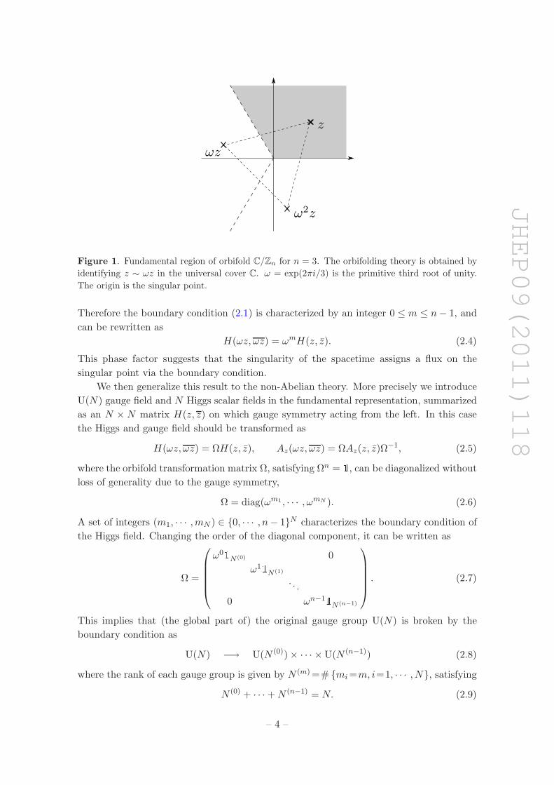
Figure 1. Fundamental region of orbifold C/Zn for n = 3. The orbifolding theory is obtained by

identifying z ∼ ωz in the universal cover C. ω = exp(2πi/3) is the primitive third root of unity.

The origin is the singular point.

Therefore the boundary condition (2.1) is characterized by an integer 0 ≤ m ≤ n − 1, and

can be rewritten as

H(ωz, ωz) = ωmH(z, z). (2.4)

This phase factor suggests that the singularity of the spacetime assigns a flux on the

singular point via the boundary condition.

We then generalize this result to the non-Abelian theory. More precisely we introduce

U(N) gauge field and N Higgs scalar fields in the fundamental representation, summarized

as an N × N matrix H(z, z) on which gauge symmetry acting from the left. In this case

the Higgs and gauge field should be transformed as

H(ωz, ωz) = ΩH(z, z), Az(ωz, ωz) = ΩAz(z, z)Ω−1, (2.5)

where the orbifold transformation matrix Ω, satisfying Ωn = 1, can be diagonalized without

loss of generality due to the gauge symmetry,

Ω = diag(ωm1 , · · · , ωmN ). (2.6)

A set of integers (m1, · · · ,mN ) ∈ 0, · · · , n− 1N characterizes the boundary condition of

the Higgs field. Changing the order of the diagonal component, it can be written as

Ω =

ω01N(0) 0

ω11N(1)

. . .

0 ωn−11N(n−1)

. (2.7)

This implies that (the global part of) the original gauge group U(N) is broken by the

boundary condition as

U(N) −→ U(N (0)) × · · · × U(N (n−1)) (2.8)

where the rank of each gauge group is given by N (m) =# mi =m, i=1, · · · , N, satisfying

N (0) + · · · + N (n−1) = N. (2.9)

– 4 –

JHEP09(2011)118

3 Moduli matrix approach

The model we study in this paper is the following,

L = Tr

[

− 1

2g2FµνFµν −DµHDµH† − λ(c1N − HH†)2

]

. (3.1)

Especially we focus on the critical coupling case λ = g2/4. In this case, the model can be

endowed with supersymmetry by adding suitable bosonic fields and fermionic superpartners

at least if we consider on the flat space. In supersymmetric context the parameter c is called

the Fayet-Illiopoulos parameter. However supersymmetry is broken in orbifold theory [53]

and so we do not discuss supersymmetry in this paper. Note that BPS properties remain

at least semi-clasically even without supersymmetry.

Then we can obtain the BPS equation from this Lagrangian,

(D1 + iD2)H = 0, F12 +g2

2(c1N − HH†) = 0. (3.2)

We then introduce the moduli matrix approach to solve this BPS equation. The first

equations can be solved as [13, 14, 47]

H(z, z) = S−1(z, z)H0(z), Az = A1 + iA2 = S−1(z, z)∂zS(z, z), (3.3)

where the holomorphic matrix H0(z) is called the moduli matrix. The rank of this matrix

is N for U(N) gauge theory, thus it becomes just a holomorphic function for the Abelian

case. Then the second equation can be recast into a gauge invariant equation, which has

a unique solution [54–56]. Therefore all moduli parameters are contained in the moduli

matrix H0(z) up to the following transformation; This construction is invariant under

(H0(z), S(z, z)) −→ (V (z)H0(z), V (z)S(z, z)) (3.4)

with V (z) ∈ GL(N, C) being holomorphic with respect to z. This is called V -transformation

and plays an important role on classifying the moduli space.

Applying the boundary condition (2.5) the moduli matrix behaves as

H0(ωz) = ΩH0(z), (3.5)

since we have ΩH = ΩS−1(Ω−1Ω)H0. Especially the boundary condition for the moduli

matrix plays an important role on studying the moduli space of vortices on the orbifold.

Since the energy of this configuration is given by

T =2πck

n= −i

c

2

∮

dz ∂z log det H0(z), (3.6)

where the integral is performed only on the fundamental region, the moduli matrix for

k-vortex solution is written as

detH0(z) =k∏

i=1

(z − zi). (3.7)

Here k is the number of vortices on the whole complex plane C and zi parametrizes the

position of the vortex. We remark the winding number k/n is different from the vortex

number k. The former one can be fractional while the latter one is always integral.

– 5 –

JHEP09(2011)118

3.1 Abelian case

We start with the simplest case k = 1. The moduli matrix, which is just a holomorphic

function in this case, can be generally written as

H0(z) =k∏

i=1

(z − zi). (3.8)

The parameter zi is regarded as a position of the i-th vortex. For k = 1, applying the

boundary condition (3.3), this function has to satisfy

ωz − z1 = ωm(z − z1). (3.9)

This condition is satisfied only if m = 1 and z1 = 0. This means that the vortex is fixed

at the singular point of C/Zn, and the boundary condition is automatically determined as

H0(ωz) = ωH0(z).

We can easily generalize this result for k < n. The boundary condition (2.4) reduces

the moduli matrix (3.8) to a trivial form

H0;n(z) = zk, (3.10)

satisfying H0(ωz) = ωkH0(z). As the case of k = 1, positions of vortices are fixed at the

origin, and thus the position moduli does not exist for k < n. This means the fractional

vortices are fixed at the origin.

We then study the case of k = n. In this case the moduli matrix (3.8) is reduced to

H0;n(z) = zn − zn1 =

n−1∏

p=0

(z − ωpz1), (3.11)

which satisfies H0(ωz) = H0(z). This configuration has only one position modulus z1 (see

figure 1).

Finally we provide the moduli matrix for generic vortex number k = ln + m ≡m (mod n),

H0;n(z) = zml∏

i=1

(zn − zni ) = zm

l∏

i=1

n−1∏

p=0

(z − ωpzi). (3.12)

We can see that this solution satisfies the boundary condition H0(ωz) = ωmH0(z). Since

there is only position, but internal moduli, the moduli space for Abelian vortices on the

orbifold is given by

MN=1,k;n = (C/Zn)[k/n] /S[k/n]. (3.13)

Here [x] denotes the largest integer not greater than x.

We have found that k fractional vortices with k < n are fixed at the orbifold singularity

of C/Zn, but once n vortices are combined together a set of them can be free from the

singularity. The same property can be found in Yang-Mills instantons [37, 38] and fractional

D-branes [48] on orbifolds .

– 6 –

JHEP09(2011)118

3.2 U(2) gauge theory

3.2.1 k = 1 vortices

We now consider the simplest non-Abelian gauge group U(2) and the orbifold C/Z2 for

convenience. The moduli matrix for k = 1 vortex in U(2) gauge theory on C is given

by [12, 16]

H(1,0)0 (z) =

(

z − z1 0

−b′ 1

)

, H(0,1)0 (z) =

(

1 −b

0 z − z1

)

. (3.14)

The corresponding orbifold transformation matrix can be simply determined by reading

the diagonal components of the moduli matrix as

Ω(1,0) =

(

−1 0

0 +1

)

, Ω(0,1) =

(

+1 0

0 −1

)

. (3.15)

On the other hand, the moduli matrices (3.14) themselves do not satisfy the boundary

condition in a consistent way because we have different expressions as follows,

H(1,0)0 (−z) =

(

−z − z1 0

−b′ 1

)

, Ω(1,0)H(1,0)0 (z) =

(

−z + z1 0

−b′ 1

)

. (3.16)

By equating them, H(1,0)0 (−z) = Ω(1,0)H

(1,0)0 (z), we have to assign z1 = 0 to satisfy

the boundary condition consistently. We obtain the same condition from the other one

H(0,1)0 (z). Thus under this orbifold projection the moduli matrix for C/Z2 theory becomes

H(1,0)0;n=2(z) =

(

z 0

−b′ 1

)

, H(0,1)0,n=2(z) =

(

1 −b

0 z

)

. (3.17)

We remark since b and b′ are related as b = 1/b′ via the V -transformation, which is regarded

as the complexified gauge transformation [16], there is only one parameter b interpreted

as the internal moduli. Therefore k = 1 fractional vortex is fixed at the singular point,

and still has the internal degree of freedom, which turns out to be a coordinate of CP1, as

the usual non-Abelian vortex. Indeed we can extract the orientation of the vortex via the

following equations [14],

H(1,0)0;n=2(z = 0)~φ(1,0) = 0, (3.18)

H(0,1)0;n=2(z = 0)~φ(0,1) = 0. (3.19)

Thus we have the orientational vectors

~φ(1,0) =

(

1

b′

)

, ~φ(0,1) =

(

b

1

)

. (3.20)

These are nothing but two patches of CP1. Thus the moduli space for k = 1 vortex solution

in U(2) gauge theory on the orbifold C/Z2 is given by

MN=2,k=1;n=2 ≃ 0 × CP1. (3.21)

– 7 –

JHEP09(2011)118

Here we introduce a useful notation to characterize the moduli matrix by using the Young

diagram as discussed in [52]: N entries of the partition correspond to the powers of the

diagonal components of the moduli matrix for U(N) gauge theory. We can always obtain

a descending ordered matrix by the V -transformation. We again remark that there is no

position moduli C/Z2. Unlike the Abelian case it still has internal moduli CP1, as in

Yang-Mills instantons on orbifolds or their resolutions to ALE spaces [37, 38].

3.2.2 k = 2 vortices

Let us study a next example, configurations of k = 2 vortices. In this case generic forms

of moduli matrices on C are given by

H(2,0)0 (z) =

(

z2 − α′z − β′ 0

−a′z − b′ 1

)

, (3.22)

H(1,1)0 (z) =

(

z − φ −η

−η z − φ

)

, (3.23)

H(0,2)0 (z) =

(

1 −az − b

0 z2 − αz − β

)

. (3.24)

The corresponding orbifold transformation matrices are given by

Ω(2,0) = Ω(0,2) =

(

+1 0

0 +1

)

, Ω(1,1) =

(

−1 0

0 −1

)

. (3.25)

Performing the orbifold projection in a similar manner, the moduli matrices are reduced to

H(2,0)0;n=2(z) =

(

z2 − β′ 0

−b′ 1

)

= H(1,0)0 (z2), (3.26)

H(1,1)0;n=2(z) =

(

z 0

0 z

)

= z12, (3.27)

H(0,2)0;n=2(z) =

(

1 −b

0 z2 − β

)

= H(0,1)0 (z2). (3.28)

We now comment on two remarkable facts. First by imposing

detH(2,0)0;n=2 = det H

(0,2)0;n=2 ⇒ β = β′ (3.29)

in order for these two of the moduli matrices, H(2,0)0;n=2 and H

(0,2)0;n=2, to describe the vortices

in the same positions as can be seen in eq. (3.7), they are almost the same as those for

k = 1 on C shown in eq. (3.14). The difference is its argument, z → z2. This means that

two vortices located at z = z1 =√

β and z = −z1 = −√β have the same internal moduli

CP1, and thus they turn out to be identical. The vortex orientation can be obtained in a

similar way as the case k = 1; from the equations

H(2,0)0;n=2(z

2 = β)~φ(2,0) = 0, (3.30)

H(0,2)0;n=2(z

2 = β′)~φ(0,2) = 0. (3.31)

– 8 –

JHEP09(2011)118

we obtain the orientational vectors

~φ(2,0) =

(

1

b′

)

, ~φ(0,2) =

(

b

1

)

. (3.32)

They are nothing but coordinates of CP1.

Second is that we cannot perform a V -transformation which connects H(1,1)0;n=2 with

H(2,0)0;n=2 or H

(0,2)0;n=2, while H

(2,0)0;n=2 and H

(0,2)0;n=2 are connected via V -transformation. This is

obvious from the fact that we cannot impose detH(1,1)0;n=2 = detH

(2,0)0;n=2(= det H

(0,2)0;n=2) except

for β = 0. Therefore the part, corresponding to H(1,1)0;n=2, is disconnected to the continuous

one connecting H(2,0)0;n=2 and H

(0,2)0;n=2 in the moduli space MN=2,k=2;n=2. In general, we

can see if the orbifold transformation matrices are different, the corresponding parts are

disconnected. Actually in this case we have Ω(2,0) = Ω(0,2) 6= Ω(1,1).

Furthermore the moduli matrix H(1,1)0;n=2 has neither of position nor internal moduli, so

that it corresponds to just an isolated point in the moduli space. The absence of internal

moduli also means that it can be regarded as an Abelian (ANO) vortex. Actually we cannot

extract the vortex orientation for this case because H(1,1)0;n=2(z = 0) = 0. Thus implying Z2

transformation of a complex coordinate z ↔ −z, the moduli space for k = 2 turns out to be

MN=2,k=2;n=2 ≃ MN=2,k=2;n=2 ∪MN=2,k=2;n=2, (3.33)

where each sector is given by

MN=2,k=2;n=2 ≃ (C/Z2) × CP1, MN=2,k=2;n=2 ≃ 0 × 0. (3.34)

3.2.3 k = 3 vortices

We then consider k = 3 vortices configurations. The generic forms of the moduli matrices

on C are written as

H(3,0)0 (z) =

(

z3 − α′z2 − β′z − γ′ 0

−a′z2 − b′z − c′ 1

)

, (3.35)

H(2,1)0 (z) =

(

z2 − η′z − κ′ 0

−λ′z − ξ′ z − ζ ′

)

, (3.36)

H(1,2)0 (z) =

(

z − ζ −λz − ξ

0 z2 − ηz − κ

)

, (3.37)

H(0,3)0 (z) =

(

1 −az2 − bz − c

0 z3 − αz2 − βz − γ

)

. (3.38)

The orbifold transformation matrices, characterizing the boundary conditions, can be sim-

ply obtained from powers of the diagonal components of the moduli matrices,

Ω(3,0) = Ω(1,2) =

(

−1 0

0 +1

)

, Ω(2,1) = Ω(0,3) =

(

+1 0

0 −1

)

. (3.39)

– 9 –

JHEP09(2011)118

We then apply the orbifold projection to the moduli matrices by removing components

whose powers are different by modulo n from that of the diagonal component in the same

row. The moduli matrices for the orbifolding theory are obtained as

H(3,0)0;n=2(z) =

(

z(z2 − β′) 0

−a′z2 − c′ 1

)

, (3.40)

H(2,1)0;n=2(z) =

(

z2 − κ′ 0

−λ′z z

)

, (3.41)

H(1,2)0;n=2(z) =

(

z −λz

0 z2 − κ

)

, (3.42)

H(0,3)0;n=2(z) =

(

1 −az2 − c

0 z(z2 − β)

)

. (3.43)

As in the previous example we have to choose β = β′ and κ = κ′ to obtain the same deter-

minant det H(3,0)0:n=2 = detH

(0,3)0:n=2 and det H

(2,1)0:n=2 = detH

(1,2)0:n=2, respectively. We can see that

H(3,0)0;n=2 and H

(0,3)0;n=2 or H

(2,1)0;n=2 and H

(1,2)0;n=2 are connected via V -transformations. However

we cannot connect a different combination, for example, H(3,0)0;n=2 and H

(2,1)0;n=2, and they are

disconnected as in the k = 2 case. Indeed the numbers of internal moduli are different: two

for the former and one for the latter. Furthermore, the orbifold transformation matrices

for them are different by comparing in the descending order. Although we have the same

orbifold transformation matrices for H(3,0)0;n=2 and H

(1,2)0;n=2, we have to compare Ω(3,0) with

Ω(2,1) because Ω(1,2) is not in the descending order.

The vortex orientations are given by

~φ(3,0) =

(

1

a′β′ + c′

)

for z2 = β, ~φ(3,0) =

(

1

c′

)

for z = 0, (3.44)

~φ(0,3) =

(

aβ + c

1

)

for z2 = β, ~φ(0,3) =

(

c

1

)

for z = 0. (3.45)

The two internal moduli for H(3,0)0;n=2 and H

(0,3)0;n=2 are interpreted as coordinates of (CP1)2

for the separated k = 2 vortices as well as the usual k = 2 configuration on C studied in [16].

When these k = 2 vortices coincide, we have β = 0. In this case the remaining orientation

is just a CP1. This situation is essentially different from the the coincident k = 2 vortices

on C where the moduli space is given by WCP2(2,1,1) ≃ CP2/Z2 [16, 57].

On the other hand, since there is the only one internal moduli for H(2,1)0;n=2 and H

(1,2)0;n=2, we

have to discuss which vortex possesses it. Then taking an asymptotic limit z ∼ ±√κ → ∞,

we have

H(2,1)0;n=2(z) −→ ±√

κ

(

2(z ∓√κ) 0

−λ′ 1

)

, (3.46)

H(1,2)0;n=2(z) −→ ±√

κ

(

1 −λ

0 2(z ∓√κ)

)

. (3.47)

– 10 –

JHEP09(2011)118

This means that an internal moduli parameter λ = 1/λ′, regarded as a coordinate of CP1,

belongs to a vortex at ±√κ. Indeed the vortex orientations at z2 = κ turn out to be

~φ(2,1) =

(

1

λ′

)

, ~φ(1,2) =

(

λ

1

)

. (3.48)

In summary, in this case the moduli space is given by

MN=2,k=3,n=2 ≃ MN=2,k=3,n=2 ∪MN=2,k=3,n=2. (3.49)

Here, for the first sector we have to write it as follows,

MN=2,k=3,n=2 ≃ Mseparate ∪Mcoincident, (3.50)

where each part

Mseparate ≃ (C∗/Z2) × (CP1)2, Mcoincident ≃ 0 × CP1 (3.51)

is glued to each other. Since the first sector is defined only when β 6= 0, we denote the

position moduli as C∗ = C\0. The second sector is simply given by

MN=2,k=3,n=2 ≃ (C/Z2) × CP1. (3.52)

3.3 U(N) gauge theory

Let us consider the moduli matrix for the generic U(N) gauge theory. Decomposing the

total vortex number, k → (k1, · · · , kN ) with k1 + · · · + kN = k and k1 ≥ k2 ≥ · · · ≥ kN , it

is written as a lower triangle matrix,

H0(z) =

zk1 + · · · 0

∗ zk2 + · · ·...

. . .. . .

∗ · · · ∗ zkN + · · ·

. (3.53)

We can perform the orbifold projection as discussed in the previous section. Writing each

decomposed vortex number as ki = lin + mi ≡ mi (mod n), the orbifold transformation

matrix is given by

Ω =

ωm1 0

ωm2

. . .

0 ωmN

. (3.54)

In order for the moduli matrix to satisfy the boundary condition consistently, we have to

remove factors whose powers are different by modulo n from that of the diagonal component

in the same row. Thus the moduli matrix (3.53) becomes

H0;n(z) =

zm1(

Z l1 + · · ·)

0

zm2f1,2(Z) zm2(

Z l2 + · · ·)

.... . .

. . .

zmN f1,N(Z) · · · zmN fN−1,N (Z) zmN

(

Z lN + · · ·)

(3.55)

– 11 –

JHEP09(2011)118

where fi,j(Z) is a polynomial of Z = zn whose degree is lower than li. Its determinant is

given by

det H0;n(z) = zm1+···+mN

l1+···+lN∏

i=1

(Z − Zi) = zm1+···+mN

l1+···+lN∏

i=1

(zn − zni ) . (3.56)

This shows that the number of the position moduli is l1+· · ·+lN , and there are m1+· · ·+mN

vortices fixed at the origin. In terms of broken gauge group the number of fixed vortices is

given byN∑

i=1

mi =n−1∑

m=0

mN (m) ≤ (n − 1)N. (3.57)

This inequality is saturated when N (0) = · · · = N (n−2) = 0, N (n−1) = N .

4 Vortex collision

Vortex collision is an important aspect of vortex dynamics. The merit for the study with

the moduli matrix is that it is directly related to coordinates of the moduli space. It has

been investigated by studying geodesics in the moduli space for vortices on C. Using a

general formula for the moduli space metric [15] head-on collision during short time has

been studied [17], and asymptotic dynamics have been studied [19] by using the asymptotic

metric for well-separated vortices [18]. Here we concentrate on collision dynamics on the

orbifold singularity by applying the method in [17].

Let us start with k = n Abelian vortices on the orbifold C/Zn. We now rewrite the

moduli matrix, just a holomorphic function, given by (3.11) as

H0;n(z, t) = Z − Ξt =

n−1∏

m=0

(z − ωmξt1/n) (4.1)

where Z = zn, Ξ = ξn and t ∈ R. After changing t → −t we have

H0;n(z,−t) = Z + Ξt =

n−1∏

m=0

(z − ωmeiπ/nξt1/n). (4.2)

Here we have an extra factor eiπ/n. This means that vortices are colliding at t = 0 at the

origin with a scattering angle θ = π/n.3 Figure 2 shows collision of Abelian vortices on the

orbifolds C/Z2 and C/Z3. The moduli matrix approach correctly reproduces the results

in [6, 58, 59] in which Zn symmetric collisions are studied in C.

Let us then discuss the non-Abelian vortex collision. This scattering property is also

found for the non-Abelian cases because it is only related to the position moduli. On the

other hand, we can see an interesting behavior of the internal moduli.

For the case of k = 2, n = 2, the vortex orientation is given by (3.32). Although

we expand the moduli matrices, (3.26) and (3.28), as β = bt and β′ = b′t, the vortex

3Such Zn symmetric collisions are also studied on hyperbolic surfaces [34].

– 12 –

JHEP09(2011)118

Figure 2. Collision of vortices on the orbifold (a) C/Z2 with θ = π/3 and (b) C/Z3 with θ = π/3.

For Zn with an odd n, vortices just look passing through the origin of the universal covering space C.

orientation is not affected at all. This means that even though each collides and scatters

with its mirror image with an angle θ = π/n = π/2 in space, but its internal moduli do

not change.

For the k = 3 case we substitute β = bt and β′ = b′t as before. The orientations, (3.44)

and (3.45), are expanded as

~φ(3,0) =

(

1

a′b′t + c′

)

for z2 = b′t, ~φ(3,0) =

(

1

c′

)

for z = 0, (4.3)

~φ(0,3) =

(

abt + c

1

)

for z2 = bt, ~φ(0,3) =

(

c

1

)

for z = 0. (4.4)

We can see that they coincide at t = 0 as

~φ(3,0) =

(

1

c′

)

, ~φ(0,3) =

(

c

1

)

, (4.5)

and go through the original direction even after the collision. This behavior is different

from the usual vortex collision on C [17]. In that case, after orientations of two colliding

vortices coincide, they change their directions in the internal space. On the other hand,

in this case, because they have only one parameter, b or b′, the direction of the time-

evolution of the internal moduli does not change. We remark that when we consider the

k = 4 configuration on C/Z2, we will see the same situation as the usual k = 2 vortex

collision on C.

5 Kahler quotient

We then discuss the Kahler quotient description of the moduli space, which has been

originally studied in terms of string theory [7] and later proven from field theory [13, 14].

It is obtained from the D-term condition for the effective theory on D-branes,

[B,B†] + II† = c1k. (5.1)

– 13 –

JHEP09(2011)118

Figure 3. Quiver diagrams for the moduli spaces of vortices on the orbifolds: (a) C and (b) C/Z3.

Here we have B ∈ Hom(V, V ), I ∈ Hom(V,W ) for two vector spaces V and W . The winding

number and the rank of the gauge group are given by their dimensions, dim V = k and

dim W = N . Since we have U(k) gauge symmetry for these data, (B, I) → (gBg−1, gI),

g ∈ U(k), the moduli space is given by

MN,k ≃ (B, I)|[B,B†] + II† = c1k/U(k). (5.2)

Let us consider the moduli space of vortices on orbifolds with respect to this Kahler

quotient description. We introduce the decomposed vector spaces in order to characterize

the representations under Zn action,

V =

n−1⊕

m=0

Vm, W =

n−1⊕

m=0

Wm. (5.3)

Their dimensions are dim Vm = k(m), dim Wm = N (m) with∑n−1

m=0 k(m) = k and∑n−1

m=0 N (m) = N . This decomposition corresponds to the gauge symmetry breaking in

eq. (2.8) due to the boundary condition as discussed in the previous section.

The isometry z → eǫz of C acts on the data as (B, I) → (eǫB, I). Therefore we have to

consider components of Bm ∈ Hom(Vm, Vm+1) and Im ∈ Hom(Vm,Wm) where we identify

Vn = V0 and Wn = W0. Figure 3 shows quiver diagrams for vector spaces. Comparing

with the ADHM method for the ALE spaces, as shown in appendix A, we can see the

quiver for the orbifold vortex theory is a half of ADHM as well as the usual case on C.

We remark that, if the two dimensional orbifold C/Γ is considered, we have to set Γ as a

finite subgroup of U(1). This means it must be the cyclic group Γ = Zn, corresponding to

the An−1 type root system.

The algebraic condition (5.1) yields

Bm−1B†m−1 − B†

mBm + ImI†m = c1k(m) , m = 0, · · · , n − 1. (5.4)

We have U(k(m)) symmetry for m-th equation. Note that as well as the ALE spaces, ifwe could resolve the singularity of the orbifold C/Zn, a different FI parameter cm wouldbe applied to each block. However such a resolution does not exist for one dimensionalorbifolds C/Zn. Thus the total moduli space is given by

M ~N,~k;n ≃

(B0, · · · , Bn−1, I0, · · · , In−1)|Bm−1B†m−1−B†

mBm+ImI†m =c1k(m) , m=0, · · · , n−1

U(k(0)) × · · · × U(k(n−1)).

(5.5)

– 14 –

JHEP09(2011)118

This moduli space is not determined by just choosing the rank of the original gauge group

and the total winding number of vortices. We have to specify a way of decomposition,

thus it is labeled by ~N = (N (0), · · · , N (n−1)) and ~k = (k(0), · · · , k(n−1)), satisfying N (0) +

· · ·+ N (n−1) = N and k(0) + · · ·+ k(n−1) = k. Since this decomposition corresponds to the

boundary condition as discussed above, the moduli spaces under different decompositions

are disconnected. The moduli space of k-vortex on the orbifold is given by

MN,k;n =⋃

| ~N |=N,|~k|=k

M ~N,~k;n. (5.6)

6 Summary and discussion

We have investigated several properties of vortices on orbifolds C/Zn. First we have con-

sidered consistent boundary conditions for fields on the orbifolds. Then we have performed

the moduli matrix approach to characterize the moduli space of vortices. Under the orb-

ifold boundary condition the moduli matrices should be determined consistently. We have

clarified some restrictions to obtain the moduli matrices for the orbifolds from the usual

ones for C, which we call the orbifold projection.

We have investigated the moduli spaces based on the orbifolded moduli matrices with

some examples. The most remarkable point which we can find in the both of Abelian and

non-Abelian cases is that the fractional vortices are just fixed at the singular point of the

orbifold, namely the origin of the complex plane. They lose position moduli but fractional

non-Abelian vortices still possess internal moduli CPN−1 for U(N) gauge theory. Indeed

a similar situation for a fractional object is observed in other models; Yang-Mills instan-

tons [37, 38] and fractional D-branes [48] on orbifolds or their resolution to ALE spaces.

In the non-Abelian theory we have the internal moduli as well as the usual vortices on

C. However, while the whole moduli space is connected via the V -transformation before

orbifolding, the moduli space for the orbifold theory can be decomposed to disconnected

parts. This decomposition is due to the gauge symmetry breaking via the boundary con-

dition. We have found that the decomposed sectors one to one correspond to the orbifold

transfomation matrices Ω in eq. (2.7), which transform fields at z and ωz, in the descending

order. Although it is similar to the theory in presence of the twisted mass term [11], an

essential difference exists between them; each sector is completely decoupled from each

other in the case of orbifolds while it is just separated by a potential in the case of twisted

mass. Accordingly, two vortex states can be connected along a string making a confined

monopole in the case of the twisted masses while it is impossible for the orbifolds.

We have also discussed vortex collision for the orbifold theory with the moduli matrix

perspective. We have shown the scattering angle is directly reflecting the orbifold structure.

Furthermore we can observe an unusual behavior of the internal moduli for the non-Abelian

vortex. The internal orientations of two vortices coincide when they are colliding, but their

behavior after the collision is different from the usual one on C.

Finally the relation to Hanany-Tong’s approach is discussed. As well as the instantons

on the orbifold, or the ALE space given by resolving its singularity, we have a similar quiver

– 15 –

JHEP09(2011)118

theory for the Kahler quotient. We have seen that it is just a half of ADHM for instantons

on the type-A orbifold C2/Zn.

Here before closing the paper, we give several discussions.

In this paper we have studied short time dynamics around the collision moment for

which we have not needed explicit metric on the moduli space, but we need it for studying a

long time behavior. The moduli space metric has been explicitly obtained for non-Abelian

vortices on C [18] and on Riemann surfaces [30] when vortices are well separated, and

dynamics and scattering have been studied on C [19]. Beyond our work it will be an

interesting and important future problem to construct an explicit metric of the moduli

space in our case of the orbifold C/Zn. One nontrivial effect will be the existence of the

fractional vortices fixed at the orbifold singularity. It does not appear in the moduli space

in some cases, but even in that case the existence of such a flux at the singularity will

change the moduli space metric. For instance, ANO vortices fixed at the singularity in

both Abelian and non-Abelian gauge theories have no moduli but the fluxes do exist there.

In this paper we have concentrated on local vortices, namely vortices in U(N) gauge

theory with NF = N fundamental scalar fields. When the number of flavor is greater than

the number of color, NF > N , vortices are called semi-local [60, 61]. However we have to be

careful on (non-)normalizability of moduli parameters in this case [62, 63]. Other extensions

would be changing gauge symmetry from U(N) to G×U(1) such as G = SO,USp [64, 65].

Let us make a comment on a relation to Yang-Mills instantons. In five dimensional

gauge theory in the Higgs phase, instantons on C2 can live stably in a vortex world-volume

in which Yang-Mills instantons are regarded as lumps or sigma model instantons [12].

It becomes Amoeba in more general on (C∗)2 [66]. In our case of the orbifold theory,

instantons live on a vortex in C × C/Zn where the vortex world-volume extends to C.

In the case of C2 we obtain usual instantons in the limit of vanishing Fayet-Iliopoulos

parameter c in which the model goes to unbroken phase. It will be interesting to study

what happens in the same limit for instantons on C × C/Zn. Also this may be related to

surface operators in the AGT relation [67].

Finally we comment on physical applications of the vortices on orbifolds. The vortex

polygon and crystal, discussed in a few body vortex system [68, 69], have a similar property

to the orbifold theory studied in this paper. We have to discuss relation between them in a

future work. Another proposal is application to the two dimensional carbon system. The

conical structure, mimicking the orbifolds C/Zn, could be obtained by manipulating the

graphene sheet or the carbon nanotube.

Acknowledgments

The authors would like to thank K. Hashimoto for valuable discussions. They are also

grateful to T. Fujimori, T. Nishioka and Y. Yoshida for useful comments. TK is supported

by Grand-in-Aid for JSPS Fellows. The work of MN is supported in part by Grant-in Aid

for Scientific Research (No. 23740198) and by the “Topological Quantum Phenomena”

Grant-in Aid for Scientific Research on Innovative Areas (No. 23103515) from the Ministry

of Education, Culture, Sports, Science and Technology (MEXT) of Japan.

– 16 –

JHEP09(2011)118

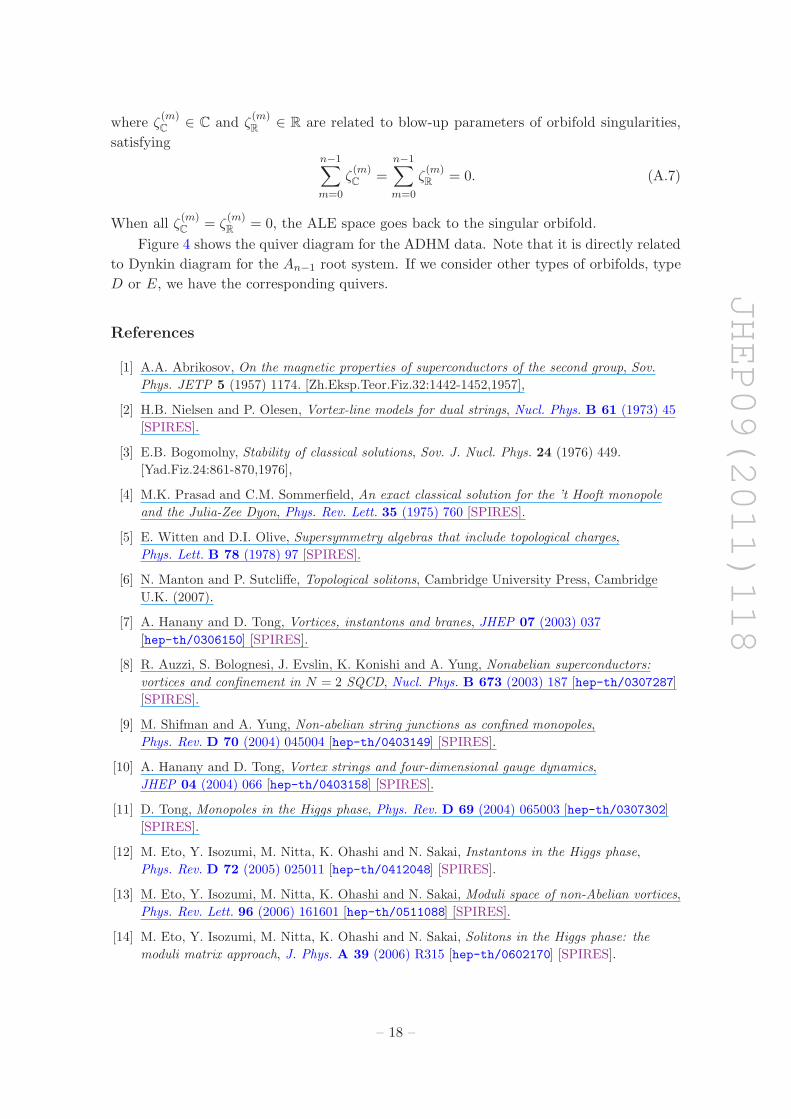
Figure 4. Quiver diagrams for the moduli spaces of instantons on the orbifolds: (a) C2 and (b)

C2/Z3.

A Instanton construction on the ALE spaces

In this appendix we comment on the ADHM construction for the ALE spaces [36–38]. First

let us start with the ADHM method without orbifolding. We now introduce the ADHM

data (B1, B2, I, J) satisfying the following ADHM equations given by

µC := [B1, B2] + IJ = 0, (A.1)

µR := [B1, B†1] + [B2, B

†2] + II† + J†J = 0, (A.2)

where B1, B2 ∈ Hom(V, V ), I ∈ Hom(W,V ) and J ∈ Hom(V,W ). The dimensions of these

vector spaces are dim V = k, dim W = N for k-instanton configuration of SU(N) gauge

theory on R4. The instanton moduli space is given by

MN,k = (B1, B2, I, J)|µC = µR = 0 /U(k). (A.3)

We have U(k) symmetry for the ADHM data such that

(B1, B2, I, J) −→ (gB1g−1, gB2g

−1, gI, Jg−1), g ∈ U(k). (A.4)

The ALE space is given by resolving the singularity of the orbifold C/Γ where Γ is

a finite subgroup of SU(2). We now discuss only the case of Γ = An−1 for simplicity.

Let (z1, z2) be a coordinate of C2, thus the orbifold C

2/Zn is obtained by identification

(z1, z2) ∼ (ωz1, ωz2) with ω = exp(2πi/n). To study how this identification affects the

ADHM equation, we then consider action of the isometry (z1, z2) → (eǫ1z1, eǫ2z2) on the

ADHM data, (B1, B2, I, J) → (eǫ1B1, eǫ2B2, I, eǫ1+ǫ2J). Decomposing the vector spaces

as well as the vortex theory (5.3) due to the irreducible representation of Zn, again these

dimensions are dim Vm = k(m), dim Wm = N (m). Then we have B1,m ∈ Hom(Vm, Vm+1),

B2,m ∈ Hom(Vm, Vm−1), Im ∈ Hom(Wm, Vm) and Jm ∈ Hom(Vm,Wm). We can write

down the ADHM equation for the ALE space in terms of these components,

B1,mB2,m+1 − B2,mB1,m−1 + ImJm = −ζ(m)C

, (A.5)

B1,m−1B†1,m−1−B†

1,mB1,m+B2,mB†2,m−B†

2,m+1B2,m+1+ImI†m−J†mJm = −ζ

(m)R

, (A.6)

– 17 –

JHEP09(2011)118

where ζ(m)C

∈ C and ζ(m)R

∈ R are related to blow-up parameters of orbifold singularities,

satisfyingn−1∑

m=0

ζ(m)C

=

n−1∑

m=0

ζ(m)R

= 0. (A.7)

When all ζ(m)C

= ζ(m)R

= 0, the ALE space goes back to the singular orbifold.

Figure 4 shows the quiver diagram for the ADHM data. Note that it is directly related

to Dynkin diagram for the An−1 root system. If we consider other types of orbifolds, type

D or E, we have the corresponding quivers.

References

[1] A.A. Abrikosov, On the magnetic properties of superconductors of the second group, Sov.

Phys. JETP 5 (1957) 1174. [Zh.Eksp.Teor.Fiz.32:1442-1452,1957],

[2] H.B. Nielsen and P. Olesen, Vortex-line models for dual strings, Nucl. Phys. B 61 (1973) 45

[SPIRES].

[3] E.B. Bogomolny, Stability of classical solutions, Sov. J. Nucl. Phys. 24 (1976) 449.

[Yad.Fiz.24:861-870,1976],

[4] M.K. Prasad and C.M. Sommerfield, An exact classical solution for the ’t Hooft monopole

and the Julia-Zee Dyon, Phys. Rev. Lett. 35 (1975) 760 [SPIRES].

[5] E. Witten and D.I. Olive, Supersymmetry algebras that include topological charges,

Phys. Lett. B 78 (1978) 97 [SPIRES].

[6] N. Manton and P. Sutcliffe, Topological solitons, Cambridge University Press, Cambridge

U.K. (2007).

[7] A. Hanany and D. Tong, Vortices, instantons and branes, JHEP 07 (2003) 037

[hep-th/0306150] [SPIRES].

[8] R. Auzzi, S. Bolognesi, J. Evslin, K. Konishi and A. Yung, Nonabelian superconductors:

vortices and confinement in N = 2 SQCD, Nucl. Phys. B 673 (2003) 187 [hep-th/0307287]

[SPIRES].

[9] M. Shifman and A. Yung, Non-abelian string junctions as confined monopoles,

Phys. Rev. D 70 (2004) 045004 [hep-th/0403149] [SPIRES].

[10] A. Hanany and D. Tong, Vortex strings and four-dimensional gauge dynamics,

JHEP 04 (2004) 066 [hep-th/0403158] [SPIRES].

[11] D. Tong, Monopoles in the Higgs phase, Phys. Rev. D 69 (2004) 065003 [hep-th/0307302]

[SPIRES].

[12] M. Eto, Y. Isozumi, M. Nitta, K. Ohashi and N. Sakai, Instantons in the Higgs phase,

Phys. Rev. D 72 (2005) 025011 [hep-th/0412048] [SPIRES].

[13] M. Eto, Y. Isozumi, M. Nitta, K. Ohashi and N. Sakai, Moduli space of non-Abelian vortices,

Phys. Rev. Lett. 96 (2006) 161601 [hep-th/0511088] [SPIRES].

[14] M. Eto, Y. Isozumi, M. Nitta, K. Ohashi and N. Sakai, Solitons in the Higgs phase: the

moduli matrix approach, J. Phys. A 39 (2006) R315 [hep-th/0602170] [SPIRES].

– 18 –

JHEP09(2011)118

[15] M. Eto, Y. Isozumi, M. Nitta, K. Ohashi and N. Sakai, Manifestly supersymmetric effective

Lagrangians on BPS solitons, Phys. Rev. D 73 (2006) 125008 [hep-th/0602289] [SPIRES].

[16] M. Eto et al., Non-Abelian vortices of higher winding numbers,

Phys. Rev. D 74 (2006) 065021 [hep-th/0607070] [SPIRES].

[17] M. Eto et al., Universal reconnection of non-Abelian cosmic strings,

Phys. Rev. Lett. 98 (2007) 091602 [hep-th/0609214] [SPIRES].

[18] T. Fujimori, G. Marmorini, M. Nitta, K. Ohashi and N. Sakai, The moduli space metric for

well-separated non-abelian vortices, Phys. Rev. D 82 (2010) 065005 [arXiv:1002.4580]

[SPIRES].

[19] M. Eto, T. Fujimori, M. Nitta, K. Ohashi and N. Sakai, Dynamics of non-abelian vortices,

arXiv:1105.1547 [SPIRES].

[20] T. Dimofte, S. Gukov and L. Hollands, Vortex counting and Lagrangian 3-manifolds,

arXiv:1006.0977 [SPIRES].

[21] Y. Yoshida, Localization of vortex partition functions in N = (2, 2) super Yang-Mills theory,

arXiv:1101.0872 [SPIRES].

[22] G. Bonelli, A. Tanzini and J. Zhao, Vertices, vortices & interacting surface operators,

arXiv:1102.0184 [SPIRES].

[23] G. Bonelli, A. Tanzini and J. Zhao, The Liouville side of the Vortex, arXiv:1107.2787

[SPIRES].

[24] A. Miyake, K. Ohta and N. Sakai, Volume of moduli space of vortex equations and

localization, arXiv:1105.2087 [SPIRES].

[25] M. Eto et al., Non-Abelian vortices on cylinder: Duality between vortices and walls,

Phys. Rev. D 73 (2006) 085008 [hep-th/0601181] [SPIRES].

[26] M. Eto et al., Statistical mechanics of vortices from D-branes and T-duality,

Nucl. Phys. B 788 (2008) 120 [hep-th/0703197] [SPIRES].

[27] G.S. Lozano, D. Marques and F.A. Schaposnik, Non-abelian vortices on the torus,

JHEP 09 (2007) 095 [arXiv:0708.2386] [SPIRES].

[28] A.D. Popov, Non-abelian vortices on Riemann surfaces: an integrable case,

Lett. Math. Phys. 84 (2008) 139 [arXiv:0801.0808] [SPIRES].

[29] J.M. Baptista, Non-abelian vortices on compact Riemann surfaces,

Commun. Math. Phys. 291 (2009) 799 [arXiv:0810.3220] [SPIRES].

[30] J.M. Baptista, On the L2-metric of vortex moduli spaces, Nucl. Phys. B 844 (2011) 308

[arXiv:1003.1296] [SPIRES].

[31] N.S. Manton and N.A. Rink, Geometry and energy of non-abelian vortices,

J. Math. Phys. 52 (2011) 043511 [arXiv:1012.3014] [SPIRES].

[32] N.S. Manton and N. Sakai, Maximally non-abelian vortices from self-dual Yang-Mills fields,

Phys. Lett. B 687 (2010) 395 [arXiv:1001.5236] [SPIRES].

[33] A.D. Popov, Integrability of vortex equations on Riemann surfaces,

Nucl. Phys. B 821 (2009) 452 [arXiv:0712.1756] [SPIRES].

[34] S. Krusch and J.M. Speight, Exact moduli space metrics for hyperbolic vortices,

J. Math. Phys. 51 (2010) 022304 [arXiv:0906.2007] [SPIRES].

– 19 –

JHEP09(2011)118

[35] N.S. Manton and N.A. Rink, Vortices on hyperbolic surfaces, J. Phys. A 43 (2010) 434024

[arXiv:0912.2058] [SPIRES].

[36] P.B. Kronheimer, The Construction of ALE spaces as hyperKahler quotients, J. Diff. Geom.

29 (1989) 665 [SPIRES].

[37] H. Nakajima, Moduli spaces of anti-self-dual connections on ALE gravitational instantons,

Invent. Math. 102 (1990) 267.

[38] P.B. Kronheimer and H. Nakajima, Yang-Mills instantons on ALE gravitational instantons,

Math. Ann. 288 (1990) 263.

[39] F. Fucito, J.F. Morales and R. Poghossian, Multi instanton calculus on ALE spaces,

Nucl. Phys. B 703 (2004) 518 [hep-th/0406243] [SPIRES].

[40] T. Kimura, Matrix model from N = 2 orbifold partition function, JHEP 09 (2011) 015

[arXiv:1105.6091] [SPIRES].

[41] L.F. Alday, D. Gaiotto and Y. Tachikawa, Liouville correlation functions from

four-dimensional gauge theories, Lett. Math. Phys. 91 (2010) 167 [arXiv:0906.3219]

[SPIRES].

[42] V. Belavin and B. Feigin, Super Liouville conformal blocks from N = 2 SU(2) quiver gauge

theories, JHEP 07 (2011) 079 [arXiv:1105.5800] [SPIRES].

[43] T. Nishioka and Y. Tachikawa, Para-Liouville/Toda central charges from M5-branes,

Phys. Rev. D 84 (2011) 046009 [arXiv:1106.1172] [SPIRES].

[44] G. Bonelli, K. Maruyoshi and A. Tanzini, Instantons on ALE spaces and super Liouville

conformal field theories, JHEP 08 (2011) 056 [arXiv:1106.2505] [SPIRES].

[45] A. Belavin, V. Belavin and M. Bershtein, Instantons and 2d superconformal field theory,

arXiv:1106.4001 [SPIRES].

[46] G. Bonelli, K. Maruyoshi and A. Tanzini, Gauge theories on ALE space and super Liouville

correlation functions, arXiv:1107.4609 [SPIRES].

[47] Y. Isozumi, M. Nitta, K. Ohashi and N. Sakai, All exact solutions of a 1/4

Bogomol’nyi-Prasad-Sommerfield equation, Phys. Rev. D 71 (2005) 065018

[hep-th/0405129] [SPIRES].

[48] M.R. Douglas and G.W. Moore, D-branes, quivers and ALE instantons, hep-th/9603167

[SPIRES].

[49] B. Collie and D. Tong, The partonic nature of instantons, JHEP 08 (2009) 006

[arXiv:0905.2267] [SPIRES].

[50] M. Eto et al., Fractional vortices and lumps, Phys. Rev. D 80 (2009) 045018

[arXiv:0905.3540] [SPIRES].

[51] M. Eto, T. Fujimori, S.B. Gudnason, M. Nitta and K. Ohashi, SO and USp Kahler and

Hyper-Kahler quotients and lumps, Nucl. Phys. B 815 (2009) 495 [arXiv:0809.2014]

[SPIRES].

[52] M. Eto et al., Group theory of non-abelian vortices, JHEP 11 (2010) 042 [arXiv:1009.4794]

[SPIRES].

[53] A. Adams, J. Polchinski and E. Silverstein, Don’t panic! Closed string tachyons in ALE

space-times, JHEP 10 (2001) 029 [hep-th/0108075] [SPIRES].

– 20 –

JHEP09(2011)118

[54] C.-S. Lin and Y. Yang, Non-Abelian multiple vortices in supersymmetric field theory,

Commun. Math. Phys. 304 (2011) 433 [SPIRES].

[55] C.-S. Lin and Y. Yang, Sharp existence and uniqueness theorems for non-Abelian multiple

vortex solutions, Nucl. Phys. B 846 (2011) 650 [SPIRES].

[56] E.H. Lieb and Y. Yang, Non-abelian vortices in supersymmetric gauge field theory via direct

methods, arXiv:1106.1626 [SPIRES].

[57] R. Auzzi, M. Shifman and A. Yung, Composite non-abelian flux tubes in N = 2 SQCD,

Phys. Rev. D 73 (2006) 105012 [hep-th/0511150]. [Erratum-ibid.D76:109901,2007],

[58] K. Arthur and J. Burzlaff, Existence theorems for pi/n vortex scattering,

Lett. Math. Phys. 36 (1996) 311 [hep-th/9503010] [SPIRES].

[59] R. MacKenzie, Remarks on gauge vortex scattering, Phys. Lett. B 352 (1995) 96

[hep-th/9503044] [SPIRES].

[60] T. Vachaspati and A. Achucarro, Semilocal cosmic strings, Phys. Rev. D 44 (1991) 3067

[SPIRES].

[61] A. Achucarro and T. Vachaspati, Semilocal and electroweak strings,

Phys. Rept. 327 (2000) 347 [hep-ph/9904229]. [Phys.Rept.327:427,2000],

[62] M. Shifman and A. Yung, Non-Abelian semilocal strings in N = 2 supersymmetric QCD,

Phys. Rev. D 73 (2006) 125012 [hep-th/0603134] [SPIRES].

[63] M. Eto et al., On the moduli space of semilocal strings and lumps,

Phys. Rev. D 76 (2007) 105002 [arXiv:0704.2218] [SPIRES].

[64] M. Eto et al., Constructing non-abelian vortices with arbitrary gauge groups,

Phys. Lett. B 669 (2008) 98 [arXiv:0802.1020] [SPIRES].

[65] M. Eto et al., Non-abelian vortices in SO(N) and USp(N) gauge theories,

JHEP 06 (2009) 004 [arXiv:0903.4471] [SPIRES].

[66] T. Fujimori, M. Nitta, K. Ohta, N. Sakai and M. Yamazaki, Intersecting solitons, amoeba

and tropical geometry, Phys. Rev. D 78 (2008) 105004 [arXiv:0805.1194] [SPIRES].

[67] H. Kanno and Y. Tachikawa, Instanton counting with a surface operator and the chain- saw

quiver, JHEP 06 (2011) 119 [arXiv:1105.0357] [SPIRES].

[68] M.R. Dhanak, Stability of a regular polygon of finite vortices, J. Fluid Mech. 234 (1992) 297.

[69] H. Aref, P.K. Newton, M.A. Stremler, T. Tokieda, and D.L. Vainchtein, Vortex crystals, Adv.

Appl. Mech. 39 (2003) 1.

– 21 –