Persistence and stability of discrete vortices in nonlinear Schr ...
34
Physica D 212 (2005) 20–53 www.elsevier.com/locate/physd Persistence and stability of discrete vortices in nonlinear Schr¨ odinger lattices D.E. Pelinovsky a , P.G. Kevrekidis b,* , D.J. Frantzeskakis c a Department of Mathematics, McMaster University, Hamilton, Ontario, Canada L8S 4K1 b Department of Mathematics, University of Massachusetts, Amherst, MA 01003-4515, USA c Department of Physics, University of Athens, Panepistimiopolis, Zografos, Athens 15784, Greece Received 5 November 2004; received in revised form 9 September 2005; accepted 16 September 2005 Available online 2 November 2005 Communicated by J. Lega Abstract We study discrete vortices in the two-dimensional nonlinear Schr¨ odinger lattice with small coupling between lattice nodes. The discrete vortices in the anti-continuum limit of zero coupling represent a finite set of excited nodes on a closed discrete contour with a non-zero charge. Using the Lyapunov–Schmidt reductions, we analyze continuation and termination of the discrete vortices for small coupling between lattice nodes. An example of a square discrete contour is considered that includes the vortex cell (also known as the off-site vortex). We classify families of symmetric and asymmetric discrete vortices that bifurcate from the anti-continuum limit. We predict analytically and confirm numerically the number of unstable eigenvalues associated with each family of such discrete vortices. c 2005 Elsevier B.V. All rights reserved. Keywords: Two-dimensional nonlinear Schr¨ odinger lattice; Lyapunov–Schmidt reductions; Discrete solitons; Discrete vortices; Persistence analysis; Stability analysis 1. Introduction Discrete systems and differential-difference equations have become topics of increasing physical and mathematical importance. The variety of physical applications where such models are relevant, and their significant differences from the mathematical theory of partial differential equations, contribute to the extensive recent interest in these topics. The applicability of such models extends to areas as diverse as nonlinear optics, atomic and soft * Corresponding author. E-mail address: [email protected] (P.G. Kevrekidis). 0167-2789/$ - see front matter c 2005 Elsevier B.V. All rights reserved. doi:10.1016/j.physd.2005.09.015
-
Upload
khangminh22 -
Category
Documents
-
view
1 -
download
0
Transcript of Persistence and stability of discrete vortices in nonlinear Schr ...

Physica D 212 (2005) 20–53www.elsevier.com/locate/physd
Persistence and stability of discrete vortices in nonlinearSchrodinger lattices
D.E. Pelinovskya, P.G. Kevrekidisb,∗, D.J. Frantzeskakisc
a Department of Mathematics, McMaster University, Hamilton, Ontario, Canada L8S 4K1b Department of Mathematics, University of Massachusetts, Amherst, MA 01003-4515, USA
c Department of Physics, University of Athens, Panepistimiopolis, Zografos, Athens 15784, Greece
Received 5 November 2004; received in revised form 9 September 2005; accepted 16 September 2005Available online 2 November 2005
Communicated by J. Lega
Abstract
We study discrete vortices in the two-dimensional nonlinear Schrodinger lattice with small coupling between lattice nodes.The discrete vortices in the anti-continuum limit of zero coupling represent a finite set of excited nodes on a closed discretecontour with a non-zero charge. Using the Lyapunov–Schmidt reductions, we analyze continuation and termination of thediscrete vortices for small coupling between lattice nodes. An example of a square discrete contour is considered that includesthe vortex cell (also known as the off-site vortex). We classify families of symmetric and asymmetric discrete vortices thatbifurcate from the anti-continuum limit. We predict analytically and confirm numerically the number of unstable eigenvaluesassociated with each family of such discrete vortices.c© 2005 Elsevier B.V. All rights reserved.
Keywords: Two-dimensional nonlinear Schrodinger lattice; Lyapunov–Schmidt reductions; Discrete solitons; Discrete vortices; Persistenceanalysis; Stability analysis
1. Introduction
Discrete systems and differential-difference equations have become topics of increasing physical andmathematical importance. The variety of physical applications where such models are relevant, and their significantdifferences from the mathematical theory of partial differential equations, contribute to the extensive recent interestin these topics. The applicability of such models extends to areas as diverse as nonlinear optics, atomic and soft
∗ Corresponding author.E-mail address: [email protected] (P.G. Kevrekidis).
0167-2789/$ - see front matter c© 2005 Elsevier B.V. All rights reserved.doi:10.1016/j.physd.2005.09.015

D.E. Pelinovsky et al. / Physica D 212 (2005) 20–53 21
condensed-matter physics, as well as biophysics. Specific details and references can be found in our first paper [1]as well as in reviews [2–7].
The present work is devoted to the existence and stability of coherent structures in two-dimensional lattices,which include both discrete solitons [6,7] and discrete vortices [8,9] (see also the pioneering work of [2] and theworks of [10,11] for Klein–Gordon lattices). These two-dimensional coherent structures have emerged recently instudies of photorefractive crystals in nonlinear optics [12,13] and droplets of optical lattices in Bose–Einsteincondensates [14,15]. A significant boost to this subject was given by the experimental realization of two-dimensional photonic crystal lattices with periodic potentials based on the ideas of [12]. As a result, discretesolitons were observed in [16,17], while more complex structures such as dipoles, soliton trains and vector solitonswere observed in [18–20].
Most recently, observations of discrete vortices were reported by two independent groups [21,22] where thefundamental vortices with topological charge one were experimentally created and detected in photorefractivecrystals. Two main examples of charge-one discrete vortices include a vortex cross (an on-site centered vortex)and a vortex cell (an off-site centered vortex). These structures were also recently predicted in a continuous two-dimensional model with the periodic potential [23].
These discoveries have stimulated further theoretical work and numerical computations. Thus, while in [9],discrete vortices of charge two were shown to be unstable, recently in [24] discrete vortices of charge three werefound to be stable. Based on the theoretical predictions of [24], further experiments on localized structures wereundertaken to unveil other interesting structures, such as the discrete soliton necklace [25]. The discrete vorticeshave been also extended to three-dimensional discrete and periodic continuum models [26–28]. Furthermore,asymmetric vortices have been recently predicted in the two-dimensional lattices in [29].
The above activity clearly signals the importance and experimental relevance of discrete solitons and vortices intwo-dimensional discrete lattices. However, most of the above-mentioned works are predominantly of experimentalor numerical nature, while the mathematical theory of existence and stability of discrete localized structures has notbeen developed to a similar extent. The only analytical method which was developed so far relied on computationsof effective action functionals (see Sections 3.2, 3.3 in [2]). It was applied to the one-dimensional discrete NLSlattice in [30] and later extended to the computations of effective Hamiltonians [31].
The aim of the present paper is to develop a categorization of discrete solitons and vortices in the discrete two-dimensional nonlinear Schrodinger (NLS) equations. We start from a well-understood limit [32] (the so-called anti-continuum case of zero coupling between the lattice nodes) and examine the persistence of the limiting solutionsfor small coupling by means of the Lyapunov–Schmidt theory. This method allows us to discuss persistence andstability of the localized structures by analyzing finite-dimensional linear eigenvalue problems. The theoreticalpredictions agree well with full numerical computations of the discrete two-dimensional NLS equation. The methodof Lyapunov–Schmidt reductions, which we employ in this paper, generalizes the pioneering method of [32], whichis based on the implicit function theorem. Very similar results on the existence and stability of two-dimensionaldiscrete vortices were obtained independently in [33] for a triangular lattice of weakly coupled Hamiltonianoscillators. The method of [33] relies on the averaging theory of effective Hamiltonians, which determine thedynamics near the discrete localized mode using Taylor series approximations.
Our main results are summarized for the simplest localized structures in Table 1. These results corroborateand extend the previously reported experimental and numerical findings. We quantify the stability of the charge-one vortex in accordance with [9,21–23], the instability of the charge-two vortex in accordance with [9,24] and thestability of the charge-three vortex in accordance with [24]. We further demonstrate the instability of all asymmetricvortices, which persist in the two-dimensional discrete lattice. Furthermore, our results can be used to extract thespectral stability of the dipole mode considered in [18] and of the soliton necklace of [25].
The paper is structured as follows. Abstract results on the existence of discrete solitons and vortices are derivedin Section 2. Persistence of localized modes for a particular square discrete contour is considered in Section 3.Stability of the persistent solutions is addressed in Section 4. Analytical results are compared to numericalcomputations in Section 5. Section 6 concludes the paper.

22 D.E. Pelinovsky et al. / Physica D 212 (2005) 20–53
Table 1The numbers of eigenvalues of linearized energy and the linearized stability problem, associated with discrete vortices in the two-dimensionalNLS lattice with small coupling between lattice nodes
Contour SM Vortex of charge L Linearized energy H Stable and unstable eigenvalues
M = 1 symmetric L = 1 n(H) = 5, p(H) = 2 Nr = 0, N+
i = 1, N−
i = 2, Nc = 0M = 2 symmetric L = 1 n(H) = 8, p(H) = 7 Nr = 1, N+
i = 0, N−
i = 0, Nc = 3M = 2 symmetric L = 2 n(H) = 10, p(H) = 5 Nr = 1, N+
i = 2, N−
i = 4, Nc = 0M = 2 symmetric L = 3 n(H) = 15, p(H) = 0 Nr = 0, N+
i = 0, N−
i = 7, Nc = 0M = 2 asymmetric L = 1 n(H) = 9, p(H) = 6 Nr = 6, N+
i = 0, N−
i = 1, Nc = 0M = 2 asymmetric L = 3 n(H) = 14, p(H) = 1 Nr = 1, N+
i = 0, N−
i = 6, Nc = 0
The numbers n(H) and p(H) stand for negative and small positive eigenvalues of H , such that n(H) + p(H) = 8M − 1. The numbersNr, N+
i , N−
i , and Nc stand for eigenvalues of the linearized stability problem with Re(λ) > 0, Im(λ) = 0; Re(λ) = 0, 0 < Im(λ) 1and positive Krein signature; Re(λ) = 0, 0 < Im(λ) 1 and negative Krein signature; and Re(λ) > 0, Im(λ) > 0 respectively, such that2Nr + 2N+
i + 2N−
i + 4Nc = 2(4M − 1). The negative index theory [1] implies that Nr + 2N−
i + 2Nc = n(H) − 1, which is confirmed bythe table data.
2. Existence of discrete vortices
We consider the discrete nonlinear Schrodinger (NLS) equation in two spatial dimensions [5]:
iun,m + ε(un+1,m + un−1,m + un,m+1 + un,m−1 − 4un,m) + |un,m |2un,m = 0, (2.1)
where un,m(t) : R+ → C, (n, m) ∈ Z2, and ε > 0 is the inverse squared step size of the lattice. The discrete NLSequation (2.1) is a Hamiltonian system with the Hamiltonian function
H =
∑(n,m)∈Z2
ε|un+1,m − un,m |2+ ε|un,m+1 − un,m |
2−
12|un,m |
4. (2.2)
Besides the conserved Hamiltonian (2.2), the discrete NLS equation conserves the squared l2-norm, called thepower:
Q =
∑(n,m)∈Z2
|un,m |2. (2.3)
The power conservation is related to the invariance of the discrete NLS equation (2.1) with respect to the gaugetransformation:
un,m(t) 7→ un,m(t)eiθ0 , ∀θ0 ∈ R. (2.4)
Time-periodic localized modes of the discrete NLS equation (2.1) take the form
un,m(t) = φn,mei(µ−4ε)t+iθ0 , φn,m ∈ C, (n, m) ∈ Z2, (2.5)
where θ0 ∈ R and µ ∈ R are parameters. Since localized modes in the focusing NLS lattice (2.1) with ε > 0 mayexist only for µ > 4ε [4] and the parameter µ is scaled out by the scaling transformation,
φn,m =√
µφn,m, ε = µε, (2.6)
the parameter µ > 0 will henceforth be set as µ = 1. In this case, the complex-valued φn,m solve the nonlineardifference equations on (n, m) ∈ Z2:
(1 − |φn,m |2)φn,m = ε
(φn+1,m + φn−1,m + φn,m+1 + φn,m−1
). (2.7)

D.E. Pelinovsky et al. / Physica D 212 (2005) 20–53 23
As ε = 0, the localized modes of the difference equations (2.7) are given by the limiting solution:
φ(0)n,m =
eiθn,m , (n, m) ∈ S,
0, (n, m) ∈ Z2\ S,
(2.8)
where S is a finite set of nodes on the lattice (n, m) ∈ Z2 and θn,m are parameters for (n, m) ∈ S. Since θ0 isarbitrary in the ansatz (2.5), we can set θn0,m0 = 0 for a particular node (n0, m0) ∈ S. Using this convention, wedefine two special types of localized modes, called discrete solitons and vortices.
Definition 2.1. The localized solution of the difference equations (2.7) with ε > 0, that has all real-valuedamplitudes φn,m , (n, m) ∈ Z2, and satisfies the limit (2.8) with all θn,m = 0, π, (n, m) ∈ S, is called a discretesoliton.
Definition 2.2. Let S be a simple closed discrete contour on the plane (n, m) ∈ Z2. The localized solution of thedifference equations (2.7) with ε > 0, that has complex-valued φn,m , (n, m) ∈ Z2, and satisfies the limit (2.8) withθn,m ∈ [0, 2π ], (n, m) ∈ S, is called a discrete vortex.
Definition 2.3. Let S be a simple closed discrete contour on the plane (n, m) ∈ Z2 such that each node (n, m) ∈ Shas exactly two adjacent nodes in vertical or horizontal directions along S. Let 1θ j be the phase difference betweentwo successive nodes in the contour S, defined according to the enumeration j = 1, 2, . . . , dim(S), such that|1θ j | ≤ π . If the phase differences 1θ j are constant along S, the discrete vortex is called symmetric. Otherwise,it is called asymmetric. The total number of 2π phase shifts across the closed contour S is called the vortex charge.
In particular, we consider the square discrete contour S = SM :
SM = (1, 1), (2, 1), . . . , (M + 1, 1), (M + 1, 2), . . . , (M + 1, M + 1),
(M, M + 1), . . . , (1, M + 1), (1, M), . . . , (1, 2) , (2.9)
where dim(SM ) = 4M . According to Definition 2.3, the contour SM for a fixed M could support symmetric andasymmetric vortices with some charge L . The simplest vortex is the symmetric charge-one vortex cell (M = L = 1:θ1,1 = 0, θ2,1 =
π2 , θ2,2 = π , θ1,2 =
3π2 ) [9,23]. Although the main formalism of our paper is developed for any
M ≥ 1, we obtain a complete set of results on persistence and stability of discrete vortices only in the casesM = 1, 2, 3, which are of most physical interest. The contours SM for M = 1 and M = 2 are shown in Fig. 1.
It follows from the general method [2,32] that the discrete solitons of the two-dimensional NLS lattice (2.7)(see Definition 2.1) can be continued to the domain 0 < ε < ε0 for some ε0 > 0. It is more complicated tofind a configuration of θn,m for (n, m) ∈ S that allows us to continue the discrete vortices (see Definition 2.2)for ε > 0. The continuation of the discrete solitons and vortices is based on the Implicit Function Theorem andthe Lyapunov–Schmidt Reduction Theorem [34,35]. Abstract results on the existence of such continuations areformulated and proved below, after the introduction of some relevant notation.
Let O(0) be a small neighborhood of ε = 0 such that O(0) = (−ε0, ε0) for some ε0 > 0. Let N = dim(S)
and T be the torus on [0, 2π]N such that θn,m for (n, m) ∈ S form a vector θ ∈ T . Let Ω = l2(Z2, C) be the
Hilbert space of square-summable complex-valued sequences φn,m(n,m)∈Z2 , equipped with the inner product andthe norm
(u, v)Ω =
∑(n,m)∈Z2
un,mvn,m, ‖u‖2l2 =
∑(n,m)∈Z2
|un,m |2 < ∞. (2.10)
Let u denote an infinite-dimensional vector in Ω that consists of components un,m for all (n, m) ∈ Z2.
Proposition 2.4. There exists a unique (discrete soliton) solution of the difference equations (2.7) in the domainε ∈ O(0) that satisfies (i) φn,m ∈ R, (n, m) ∈ Z2 and (ii) limε→0 φn,m = φ
(0)n,m , where φ
(0)n,m is given by (2.8) with
θn,m = 0, π, (n, m) ∈ S. The solution φ(ε) is analytic in ε ∈ O(0).

24 D.E. Pelinovsky et al. / Physica D 212 (2005) 20–53
Fig. 1. Examples of the simple closed square contour SM for M = 1 and M = 2.
Proof. Assume that φn,m ∈ R for all (n, m) ∈ Z2. The difference equations (2.7) are rewritten as zeros of thenonlinear vector-valued function:
fn,m(φ, ε) = (1 − φ2n,m)φn,m − ε
(φn+1,m + φn−1,m + φn,m+1 + φn,m−1
)= 0. (2.11)
The mapping f : Ω ×O(0) 7→ Ω is C1 on φ ∈ Ω and has a bounded continuous Frechet derivative, given by
Ln,m =
(1 − 3φ2
n,m
)− ε
(s+1,0 + s−1,0 + s0,+1 + s0,−1
), (2.12)
where sn′,m′ is the shift operator, such that sn′,m′un,m = un+n′,m+m′ . It is obvious that
f(φ(0), 0) = 0, ker(L(0)) = ∅, (2.13)
where φ(0) is the discrete soliton for ε = 0 (see Definition 2.1) and L(0) is the operator L computed at φ = φ(0)
and ε = 0. It follows from (2.12) and (2.13) that L(0): Ω 7→ Ω has a bounded inverse. By the Implicit Function
Theorem [35, Appendix 1], there exists a local mapping φ : O(0) → Ω , such that φ(ε) is at least continuous in

D.E. Pelinovsky et al. / Physica D 212 (2005) 20–53 25
ε ∈ O(0) and φ(0)= φ(0). Moreover, since f(φ, ε) is analytic in ε ∈ O(0), then φ(ε) is analytic in ε ∈ O(0)
[34, Chapter 2.2].
Remark 2.5. Proposition 2.4 does not exclude a possibility of continuation of the limiting solution (2.8) withθn,m = 0, π for all (n, m) ∈ S to the complex-valued solution φ(ε) in ε ∈ O(0).
Proposition 2.6. There exists a vector-valued function g : T ×O(0) 7→ RN such that the limiting solution (2.8) iscontinued to the domain ε ∈ O(0) if and only if θ ∈ T is a root of g(θ , ε) = 0 in ε ∈ O(0). Moreover, the functiong(θ , ε) is analytic in ε ∈ O(0) and g(θ , 0) = 0 for any θ ∈ T .
Proof. When φn,m ∈ C for some (n, m) ∈ Z2, the difference equations (2.7) are complemented by the complexconjugate equations in the abstract form:
f(φ, φ, ε) = 0, f(φ, φ, ε) = 0. (2.14)
Taking the Frechet derivative of f(φ, φ, ε) with respect to φ and φ, we compute the linearization operator H forthe difference equations (2.7):
Hn,m =
(1 − 2|φn,m |
2−φ2
n,m−φ2
n,m 1 − 2|φn,m |2
)− ε(s+1,0 + s−1,0 + s0,+1 + s0,−1)
(1 00 1
). (2.15)
Let H(0)= H(φ(0), 0). It is clear that H(0)
: Ω × Ω 7→ Ω × Ω is a self-adjoint Fredholm operator of index zerowith dim ker(H(0)) = N . Moreover, eigenvectors of ker(H(0)) renormalize the parameters θn,m for (n, m) ∈ S inthe limiting solution (2.8). By the Lyapunov Reduction Theorem [35, Chapter 7.1], there exists a decompositionΩ = ker(H(0)) ⊕ ω such that g(θ , ε) is defined in terms of the projections to ker(H(0)). Let en,m(n,m)∈S be a setof N linearly independent eigenvectors in the kernel ofH(0). It follows from the representation,
H(0)n,m = −
(1 e2iθn,m
e−2iθn,m 1
), (n, m) ∈ S, (2.16)
that each eigenvector en,m in the set en,m(n,m)∈S has the only non-zero element (eiθn,m , −e−iθn,m )T at the (n, m)-thposition of (u, w) ∈ Ω × Ω . By projections of the nonlinear equations (2.14) to ker(H(0)), we derive an implicitrepresentation for the functions g(θ , ε):
(n, m) ∈ S : 2ign,m(θ , ε) = (1 − |φn,m |2)(
e−iθn,m φn,m − eiθn,m φn,m
)− εe−iθn,m
(φn+1,m + φn−1,m + φn,m+1 + φn,m−1
)+ εeiθn,m
(φn+1,m + φn−1,m + φn,m+1 + φn,m−1
), (2.17)
where the factor (2i) is introduced for convenient notation. Let φn,m = eiθn,m un,m for (n, m) ∈ S and φn,m = un,mfor (n, m) ∈ Z2
\ S. Since eigenvectors of ker(H(0)) are excluded from the solution φ in ω ⊂ Ω , we have un,m ∈ Rfor (n, m) ∈ S such that
(n, m) ∈ S : −2ign,m(θ , ε) = εe−iθn,m(φn+1,m + φn−1,m + φn,m+1 + φn,m−1
)− εeiθn,m
(φn+1,m + φn−1,m + φn,m+1 + φn,m−1
)(2.18)
and g(θ , 0) = 0 for any θ ∈ T . Since f(φ, φ, ε) is analytic in ε ∈ O(0), then g(θ , ε) is analytic in ε ∈ O(0)
[35, Appendix 3].
Corollary 2.7. The function g(θ , ε) can be expanded into convergent Taylor series in O(0):
g(θ , ε) =
∞∑k=1
εkg(k)(θ), g(k)(θ) =1k!
∂kε g(θ , 0). (2.19)

26 D.E. Pelinovsky et al. / Physica D 212 (2005) 20–53
If the root θ(ε) of g(θ , ε) = 0 is analytic in ε ∈ O(0), then the solution φ(ε) is analytic in ε ∈ O(0) such that
φ(ε) = φ(0)+
∞∑k=1
εkφ(k), (2.20)
where φ(0) is given by (2.8).
Lemma 2.8. Let θ(ε) be a root of g(θ , ε) = 0 in ε ∈ O(0). An arbitrary shift θ(ε) + θ0p0, where θ0 ∈ R andp0 = (1, 1, . . . , 1)T, gives a one-parameter family of roots of g(θ , ε) = 0 for the same ε.
Proof. The statement follows from the symmetry of the difference equations (2.7) with respect to gaugetransformation (2.4) (see [35, Chapter 7.3]).
Proposition 2.9. Let θ∗ be the root of g(1)(θ) = 0 and M1 be the Jacobian matrix of g(1)(θ) at θ = θ∗. If thematrixM1 has a simple zero eigenvalue, there exists a unique (modulo gauge transformation) analytic continuationof the limiting solution (2.8) to the domain ε ∈ O(0).
Proof. By Lemma 2.8, the matrixM1 always has a non-empty kernel with the eigenvector p0 = (1, 1, . . . , 1) dueto gauge transformation. Let X0 be the constrained subspace of CN :
X0 = u ∈ CN: (p0, u) = 0. (2.21)
If the matrix M1 is non-singular in the subspace X0, then there exists a unique (modulo the shift) analyticcontinuation of the root θ∗ in ε ∈ O(0) by the Implicit Function Theorem, applied to the nonlinear equationg(θ , ε) = 0 [35, Appendix 1].
Proposition 2.10. Let θ∗ be a (1 + d)-parameter solution of g(1)(θ) = 0 and M1 have a zero eigenvalue ofmultiplicity (1 + d), where 1 ≤ d ≤ N − 1. Let g(2)(θ∗) = · · · = g(K−1)(θ∗) = 0 but g(K )(θ∗) 6= 0. The limitingsolution (2.8) can be continued in the domain ε ∈ O(0) only if g(K )(θ∗) is orthogonal to ker(M1).
Proof. Let p0 and pldl=1 be eigenvectors of ker(M1). We define the constrained subspace of X0:
Xd = u ∈ X0 : (pl , u) = 0, l = 1, . . . , d. (2.22)
If g(K )(θ∗) 6∈ Xd , the Lyapunov–Schmidt Reduction Theorem in finite dimensions [35, Chapter 1.3] shows thatthe solution θ∗ cannot be continued in ε ∈ O(0).
Proposition 2.6 gives an abstract formulation of the continuation problem for the limiting solution (2.8) forε 6= 0. Proposition 2.9 gives a sufficient condition for existence and uniqueness (up to gauge invariance) of suchcontinuations. Proposition 2.10 gives a sufficient condition for termination of multi-parameter solutions. Particularapplications of Propositions 2.6, 2.9 and 2.10 are limited by the complexity of the set S in the limiting solution(2.8), since computations of the vector-valued function g(1)(θ), g(2)(θ), . . . , g(K )(θ) and the Jacobian matrix M1could be technically involved. We apply the abstract results of Propositions 2.6, 2.9 and 2.10 to the square discretecontour SM , defined in (2.9).
3. Persistence of discrete vortices
We consider discrete solitons and vortices on the contour SM defined by (2.9). Let the set θ j correspond to theordered contour SM , starting at θ1 = θ1,1, θ2 = θ2,1 and ending at θN = θ1,2, where N = 4M . In what follows, weuse the periodic boundary conditions for θ j on the circle from j = 1 to j = N , such that θ0 = θN , θ1 = θN+1, andso on.

D.E. Pelinovsky et al. / Physica D 212 (2005) 20–53 27
The discrete vortex has the charge L if the phase differences 1θ j between two consecutive nodes add up to2π L along the discrete contour SM , where 1θ j is defined within the fundamental branch |1θ j | ≤ π . By gaugetransformation, we can always set θ1 = 0 for convenience. We will also choose θ2 = θ with 0 ≤ θ ≤ π forconvenience, which corresponds to discrete vortices with L ≥ 0.
3.1. Solutions of the first-order reductions
Substituting the limiting solution φ(0)n,m in the bifurcation function (2.18), we find that g(1)(θ) in the Taylor series
(2.19) is non-zero for the contour SM and it takes the form
g(1)j (θ) = sin(θ j − θ j+1) + sin(θ j − θ j−1), 1 ≤ j ≤ N . (3.1)
The bifurcation equations g(1)(θ) = 0 are rewritten as a system of N nonlinear equations for N parametersθ1, θ2, . . . , θN as follows:
sin(θ2 − θ1) = sin(θ3 − θ2) = · · · = sin(θN − θN−1) = sin(θ1 − θN ). (3.2)
We classify all solutions of the bifurcation equations (3.2) and give explicit examples for M = 1 and M = 2.
Proposition 3.1. Let a j = cos(θ j+1 − θ j ) for 1 ≤ j ≤ N, such that θ1 = 0, θ2 = θ , and θN+1 = 2π L, whereN = 4M, 0 ≤ θ ≤ π and L is the vortex charge. All solutions of the bifurcation equations (3.2) reduce to fourfamilies:
(i) Discrete solitons with θ = 0, π and
θ j = 0, π, 3 ≤ j ≤ N , (3.3)
such that the set a j Nj=1 includes l coefficients a j = 1 and N − l coefficients a j = −1, where 0 ≤ l ≤ N.
(ii) Symmetric vortices of charge L with θ =π L2M , where 1 ≤ L ≤ 2M − 1, and
θ j =π L( j − 1)
2M, 3 ≤ j ≤ N , (3.4)
such that all N coefficients are the same: a j = a = cos(
π L2M
).
(iii) One-parameter families of asymmetric vortices of charge L = M with 0 < θ < π and
θ j+1 − θ j =
θ
π − θ
mod (2π), 2 ≤ j ≤ N , (3.5)
such that the set a j Nj=1 includes 2M coefficients a j = cos θ and 2M coefficients a j = − cos θ .
(iv) Zero-parameter asymmetric vortices of charge L 6= M and
θ = θ∗ =π
2
(n + 2L − 4M
n − 2M
), 1 ≤ n ≤ N − 1, n 6= 2M, (3.6)
such that the set a j Nj=1 includes n coefficients a j = cos θ∗ and N − n coefficients a j = − cos θ∗ and the
family (iv) does not reduce to any of the families (i)–(iii).
Proof. All solutions of the bifurcation equations (3.2) are given by the binary choice equations (3.5) in the tworoots of the sine function on θ ∈ [0, 2π ], where the first choice gives a j = cos θ and the second choice givesa j = − cos θ . Let us assume that there are in total n first choices and N − n second choices, where 1 ≤ n ≤ N .Then, we have
θN+1 = nθ + (N − n)(π − θ) = (2n − N )θ + (N − n)π = 2π L ,

28 D.E. Pelinovsky et al. / Physica D 212 (2005) 20–53
where L is the integer charge of the discrete vortex. There are only two solutions of the above equation. When θ
is an arbitrary parameter, we have n =N2 = 2M and L = M , which gives the one-parameter family (iii). When
θ = θ∗ is fixed, we have
θ∗ =π
2
(n + 2L − 4M
n − 2M
).
When n = N − 2L , we have the family (i) with N − 2L phases θ j = 0 and 2L phases θ j = π . Since the chargeis not assigned to discrete solitons, parameter L could be half-integer: L = (N − l)/2, where 0 ≤ l ≤ N . Whenn = 4M , we have the family (ii) for any 1 ≤ L ≤ 2M −1. Other choices of n, which are irreducible to the families(i)–(iii), produce the family (iv).
Remark 3.2. The one-parameter family (iii) connects special solutions of the families (i) and (ii). When θ = 0 andθ = π , the family (iii) reduces to the family (i) with l = 2M . When θ =
π2 , the family (iii) reduces to the family
(ii) with L = M . We shall call the corresponding solutions of family (i) the super-symmetric soliton and those offamily (ii) the super-symmetric vortex.
Remark 3.3. There exist N1 = 2N−1 solutions of family (i), N2 = 2M − 1 solutions of family (ii), and N3solutions of family (iii), where
N3 = 2N−1−
2M−1∑k=0
N !
k!(N − k)!. (3.7)
The number N4 of solutions of family (iv) cannot be computed in general. We consider such solutions only in theexplicit examples of M = 1 and M = 2.
Example (M = 1 (N = 4)). There are N1 = 8 solutions of family (i), N2 = 1 solution of family (ii), N3 = 3solutions of family (iii), and no solutions of family (iv). The only symmetric vortex is the vortex cell with L = 1and θ =
π2 . The three one-parameter asymmetric vortices are given explicitly by
(a) θ1 = 0, θ2 = θ, θ3 = π, θ4 = π + θ (3.8)
(b) θ1 = 0, θ2 = θ, θ3 = 2θ, θ4 = π + θ (3.9)
(c) θ1 = 0, θ2 = θ, θ3 = π, θ4 = 2π − θ. (3.10)
Example (M = 2 (N = 8)). There are N1 = 128 solutions of family (i), N2 = 3 solutions of family (ii),N3 = 35 solutions of family (iii), and N4 = 14 solutions of family (iv). The three symmetric vortices havecharge L = 1 (θ =
π4 ), L = 2 (θ =
π2 ), and L = 3 (θ =
3π4 ). The one-parameter asymmetric vortices
include 35 combinations of four upper choices and four lower choices in (3.5), starting with the following threesolutions:
(a) θ1 = 0, θ2 = θ, θ3 = 2θ, θ4 = 3θ, θ5 = 4θ, θ6 = π + 3θ, θ7 = 2π + 2θ, θ8 = 3π + θ,
(b) θ1 = 0, θ2 = θ, θ3 = 2θ, θ4 = 3θ, θ5 = π + 2θ, θ6 = π + 3θ, θ7 = 2π + 2θ, θ8 = 3π + θ,
(c) θ1 = 0, θ2 = θ, θ3 = 2θ, θ4 = 3θ, θ5 = π + 2θ, θ6 = 2π + θ, θ7 = 2π + 2θ, θ8 = 3π + θ,
and so on. The zero-parameter asymmetric vortices include seven combinations of vortices with L = 1 for sevenphase differences π
6 and one phase difference 5π6 and seven combinations of vortices with L = 3 for one phase
difference π6 and seven phase differences 5π
6 .

D.E. Pelinovsky et al. / Physica D 212 (2005) 20–53 29
3.2. Continuation of solutions of the first-order reductions
We compute the Jacobian matrixM1 from the bifurcation function g(1)(θ), given in (3.1):
(M1)i, j =
cos(θ j+1 − θ j ) + cos(θ j−1 − θ j ), i = j− cos(θ j − θi ), i = j ± 10, |i − j | ≥ 2
(3.11)
subject to the periodic boundary conditions. The structure of the matrix M1 is defined by the coefficientsa j = cos(θ j+1 − θ j ) for 1 ≤ j ≤ N . The same type of matrices occurs in the perturbation theory of continuousmulti-pulse solitons in coupled NLS equations [36]. Three technical results establish the location of the eigenvaluesof the matrixM1.
Lemma 3.4. Let n0, z0, and p0 be the numbers of negative, zero, and positive terms of a j = cos(θ j+1 − θ j ),1 ≤ j ≤ N, such that n0 + z0 + p0 = N. Let n(M1), z(M1), and p(M1) be the numbers of negative, zero, andpositive eigenvalues of the matrixM1, defined by (3.11). Assume that z0 = 0 and write
A1 =
N∑i=1
∏j 6=i
a j =
(N∏
i=1
ai
) (N∑
i=1
1ai
). (3.12)
If A1 6= 0, then z(M1) = 1, and either n(M1) = n0 − 1, p(M1) = p0 or n(M1) = n0, p(M1) = p0 − 1.Moreover, n(M1) is even if A1 > 0 and is odd if A1 < 0. If A1 = 0, then z(M1) ≥ 2.
Proof. The first statement follows from [36, Appendix A]. Let the determinant equation be D(λ) = det(M1 −
λI ) = 0. By induction arguments in [36,37], it can be found that D(0) = 0 and D′(0) = −N A1. On the otherhand, D′(0) = −λ1λ2 · · · λN−1, where λN = 0 (which exists always with the eigenvector p0 = (1, 1, . . . , 1)T; seeProposition 2.9). Then, it is clear that (−1)n(M1) = sign(A1). When A1 = 0, at least one more eigenvalue is zero,such that z(M1) ≥ 2.
Lemma 3.5. Let all coefficients a j = cos(θ j+1 − θ j ), 1 ≤ j ≤ N, be the same: a j = a. Eigenvalues of the matrixM1 are computed explicitly as follows:
λn = 4a sin2 πn
N, 1 ≤ n ≤ N . (3.13)
Proof. When a j = a, 1 ≤ j ≤ N , the eigenvalue problem for the matrixM1 takes the form of the linear differenceequations with constant coefficients:
a(2x j − x j+1 − x j−1
)= λx j , x0 = xN , x1 = xN+1, (3.14)
The discrete Fourier mode x j = exp(
i 2π jnN
)for 1 ≤ j, n ≤ N results in the solution (3.13).
Lemma 3.6. Let all coefficients a j = cos(θ j+1 − θ j ), 1 ≤ j ≤ N, alternate the sign as a j = (−1) j a, whereN = 4M. Eigenvalues of the matrixM1 are computed explicitly as follows:
λn = −λn+2M = 2a sinπn
2M, 1 ≤ n ≤ 2M, (3.15)
such that n(M1) = 2M − 1, z(M1) = 2, and p(M1) = 2M − 1. These numbers do not change if the set a j Nj=1
is obtained from the sign-alternating set (−1) j aNj=1 by permutations.
Proof. When a j = (−1) j a, 1 ≤ j ≤ 4M , the eigenvalue problem for the matrix M1 takes the form of a coupledsystem of linear difference equations with constant coefficients:
a(y j − y j−1
)= λx j , a
(x j − x j+1
)= λy j , 1 ≤ j ≤ 2M, (3.16)
subject to the periodic boundary conditions: x1 = x2M+1 and y0 = y2M . The discrete Fourier mode x j =

30 D.E. Pelinovsky et al. / Physica D 212 (2005) 20–53
x0 exp(
i 2π jn2M
)and y j = y0 exp
(i 2π jn
2M
)for 1 ≤ j, n ≤ 2M results in the solution (3.15). In this case, we have
n(M1) = 2M − 1, z(M1) = 2, and p(M1) = 2M − 1, such that D(0) = D′(0) = 0 and D′′(0) < 0 in thedeterminant equation D(λ) = det(M1 − λI ). In order to prove that z(M1) = 2 remains invariant with respect topermutations of the sign-alternating set (−1) j a
Nj=1, we find with the aid of Mathematica that
D′′(0) =
(N∏
i=1
ai
) (αN
(N−1∑i=1
1ai ai+1
+1
a1aN
)+ βN
(N−2∑i=1
N∑l=i+2
1ai al
−1
a1aN
)), (3.17)
where 0 < αN < βN are numerical coefficients. Let A∗ denote the sign-alternating set (−1) j aNj=1 and A denote
a set obtained from A∗ by permutations. It is clear that(N−1∑i=1
1ai ai+1
+1
a1aN
)A∗
≤
(N−1∑i=1
1ai ai+1
+1
a1aN
)A
and (N−1∑i=1
N∑l=i+1
1ai al
)A∗
=
(N−1∑i=1
N∑l=i+1
1ai al
)A
.
Therefore, the expression in brackets in (3.17) can be estimated as follows:
(αN − βN )
(N−1∑i=1
1ai ai+1
+1
a1aN
)A
+ βN
(N−1∑i=1
N∑l=i+1
1ai al
)A
≤ (αN − βN )
(N−1∑i=1
1ai ai+1
+1
a1aN
)A∗
+ βN
(N−1∑i=1
N∑l=i+1
1ai al
)A∗
< 0,
where the last inequality follows from the fact that D′′(0) < 0 for A∗. Therefore, z(M1) = 2 for the setA. Combining it with estimates from [36, Appendix A], we have n(M1) = p(M1) = 2M − 1 for theset A.
Using Lemmas 3.4–3.6, we classify continuations of solutions of the first-order reductions (see families (i)–(iv)of Proposition 3.1).
For family (i), excluding the case of super-symmetric solitons (see Remark 3.2), the numbers of positive andnegative signs of a j are different, such that the conditions z0 = 0 and A1 6= 0 are satisfied in Lemma 3.4,and hence z(M1) = 1. By Proposition 2.9, the family (i) has a unique continuation to discrete solitons (seeDefinition 2.1). This result agrees with Proposition 2.4. Continuations described in Remark 2.5 are only possiblefor super-symmetric solitons.
For family (ii), all coefficients a j are the same: a j = a = cos(
π L2M
), 1 ≤ j ≤ N . By Lemma 3.5, there is
always a zero eigenvalue (λN = 0), while the remaining (N − 1) eigenvalues are all positive for a > 0 (when1 ≤ L ≤ M − 1), negative for a < 0 (when M + 1 ≤ L ≤ 2M − 1), and zero for a = 0 (when L = M).By Proposition 2.9, the family (ii), excluding the case of super-symmetric vortices (see Remark 3.2), has a uniquecontinuation to symmetric vortices with charge L , where 1 ≤ L ≤ 2M − 1 and L 6= M (see Definitions 2.2 and2.3).
For family (iii), there are 2M coefficients a j = cos θ and 2M coefficients a j = − cos θ , which are non-zerofor θ 6=
π2 . By Lemma 3.6, we have n(M1) = 2M − 1, z(M1) = 2, and p(M1) = 2M − 1. The additional

D.E. Pelinovsky et al. / Physica D 212 (2005) 20–53 31
zero eigenvalue is related to the derivative of the family of the asymmetric discrete vortices (3.5) with respect tothe parameter θ . Therefore, continuations of family (iii) of asymmetric vortices, including the particular cases ofsuper-symmetric solitons of family (i) and super-symmetric vortices of family (ii), must be considered beyond thefirst-order reductions.
For family (iv), since n 6= 2M , the conditions z0 = 0 and A1 6= 0 are satisfied in Lemma 3.4, and hencez(M1) = 1. By Proposition 2.9, the family (iv) has a unique continuation to asymmetric vortices for ε 6= 0.
3.3. Continuation of solutions to the second-order reductions
Results of the first-order reductions are insufficient for concluding persistence of the asymmetric vortices offamily (iii), including the super-symmetric soliton of family (i) and the super-symmetric vortex of family (ii).Therefore, we continue the bifurcation function g(θ , ε) to the second order of ε in the Taylor series (2.19).It follows from (2.7) that the first-order correction of the Taylor series (2.20) satisfies the inhomogeneousproblem:
(1 − 2|φ(0)n,m |
2)φ(1)n,m − φ(0)2
n,m φ(1)n,m = φ
(0)n+1,m + φ
(0)n−1,m + φ
(0)n,m+1 + φ
(0)n,m−1. (3.18)
We define the solution of the inhomogeneous problem (3.18) in ω ⊂ Ω , so that the homogeneous solutions inker(H(0)) are removed from the solution φ(1). This is equivalent to the constraint: φn,m = un,meiθn,m , un,m ∈ R,for all (n, m) ∈ SM . We develop computations for three distinct cases: M = 1, M = 2 and M ≥ 3. This separationis due to the special structure of the discrete contours SM .
Case M = 1: The inhomogeneous problem (3.18) has a unique solution φ(1)∈ ω ⊂ Ω :
φ(1)n,m = −
12
[cos(θ j−1 − θ j ) + cos(θ j+1 − θ j )
]eiθ j , (3.19)
where the index j enumerates the node (n, m) on the contour SM ,
φ(1)n,m = eiθ j , (3.20)
where the node (n, m) is adjacent to the j-th node on the contour SM , while φ(1)n,m is zero for all remaining nodes.
By substituting the first-order correction term φ(1)n,m into the bifurcation function (2.18), we find the correction term
g(2)(θ) in the Taylor series (2.19):
g(2)j (θ) =
12
sin(θ j+1 − θ j )[cos(θ j − θ j+1) + cos(θ j+2 − θ j+1)
]+
12
sin(θ j−1 − θ j )[cos(θ j − θ j−1) + cos(θ j−2 − θ j−1)
], 1 ≤ j ≤ N . (3.21)
We compute the vector g2 = g(2)(θ) at the asymmetric vortex solutions (3.8)–(3.10):
(a) g2 =
0000
, (b) g2 =
20
−20
sin θ cos θ, (c) g2 =
0
−202
sin θ cos θ.
The kernel ofM1 is two-dimensional with the eigenvectors p0 = (1, 1, 1, 1)T and p1. The eigenvector p1 is relatedto derivatives of the solutions (3.8)–(3.10) in θ :
(a) p1 =
0101
, (b) p1 =
0121
, (c) p1 =
010
−1
.

32 D.E. Pelinovsky et al. / Physica D 212 (2005) 20–53
The Fredholm alternative (p1, g2) = 0 is satisfied for the solution (a) but fails for the solutions (b) and (c), unlessθ = 0, π
2 , π. The latter cases are included in the definitions of super-symmetric discrete solitons and vortices(see Remark 3.2). By Proposition 2.10 with K = 2, the solutions (b) and (c) cannot be continued in ε 6= 0, whilethe solution (a) can be continued up to the second-order reductions.
Case M = 2: The solution φ(1)∈ ω ⊂ Ω of the inhomogeneous problem (3.18) is given by (3.19) and (3.20),
except for the center node (2, 2), where
φ(1)2,2 = eiθ2 + eiθ4 + eiθ6 + eiθ8 . (3.22)
The correction term g(2)(θ) is given by (3.21) but the even entries are modified as follows:
g(2)j (θ) → g(2)
j (θ) + sin(θ j − θ j−2) + sin(θ j − θ j+2) + sin(θ j − θ j+4), j = 2, 4, 6, 8. (3.23)
The vector g2 = g(2)(θ) can be computed for each of 35 one-parameter asymmetric vortex solutions, starting withthe first three solutions:
(a) g2 =
210
−1−2−101
sin θ cos θ, (b) g2 =
21
−1−10
−1−11
sin θ cos θ, (c) g2 =
21
−1−201
−10
sin θ cos θ.
The second eigenvector p1 of the kernel ofM1 is related to derivatives of the family in θ , e.g.
(a) p1 =
01234321
, (b) p1 =
01232321
, (c) p1 =
01232121
.
Assuming that θ 6= 0, π2 , π, the Fredholm alternative condition (p1, g2) = 0 fails for all solutions of family (iii)
but one. The only solution of family (iii), where g2 = 0, is characterized by the alternating signs of coefficientsa j = cos(θ j+1 − θ j ) for 1 ≤ j ≤ N .
Case M ≥ 3: The solution φ(1)∈ ω ⊂ Ω of the inhomogeneous problem (3.18) is given by (3.19) and (3.20),
except for the four interior corner nodes (2, 2),(M, 2),(M, M), and (2, M), where
φ(1)n,m = eiθ j−1 + eiθ j+1 , j = 1, M + 1, 2M + 1, 3M + 1. (3.24)
The correction term g(2)(θ) is given by (3.21), except for the adjacent entries to the four corner nodes on the contourSM : (1, 1), (1, M + 1), (M + 1, M + 1), and (M + 1, 1), which are modified by
g(2)j (θ) → g(2)
j (θ) + sin(θ j − θ j−2), j = 2, M + 2, 2M + 2, 3M + 2,
g(2)j (θ) → g(2)
j (θ) + sin(θ j − θ j+2), j = M, 2M, 3M, 4M. (3.25)

D.E. Pelinovsky et al. / Physica D 212 (2005) 20–53 33
For any M ≥ 3, there is a solution of family (iii), where g2 = 0, which is characterized by the alternating signs ofcoefficients a j = cos(θ j+1 − θ j ) for 1 ≤ j ≤ N . In the case M = 3, we have checked that all other solutions offamily (iii) have (p1, g2) 6= 0 and hence terminate at the second-order reductions.
By Proposition 2.10 with K = 2, all asymmetric vortices of family (iii), except for the sign-alternating seta j = cos(θ j+1 − θ j ) = (−1) j+1 cos θ , 1 ≤ j ≤ N , cannot be continued to ε 6= 0 for M = 1, 2, 3. The onlysolution which can be continued up to the second-order reductions has the explicit form
θ4 j−3 = 2π( j − 1), θ4 j−2 = θ4 j−3 + θ, θ4 j−1 = θ4 j−3 + π, θ4 j = θ4 j−3 + π + θ, (3.26)
where 1 ≤ j ≤ M and 0 ≤ θ ≤ π . This solution includes two particular cases of super-symmetric solitons offamily (i) for θ = 0 and θ = π and super-symmetric vortices of family (ii) for θ =
π2 . Continuation of the solution
(3.26) must be considered beyond the second-order reductions.Based on these computations, we also consider continuations of super-symmetric solitons of family (i).
Let M2 be the Jacobian matrix computed from the bifurcation function g(2)(θ), given in (3.21), (3.23) and(3.25). Since (p1, g2) 6= 0 for θ 6= 0, π
2 , π, except for the case of the sign-alternating set (−1) j aNj=1,
it follows from regular perturbation theory that (p1,M2p1) 6= 0. Therefore, the second zero eigenvalueof M1 bifurcates off zero for the matrix M1 + εM2. By Proposition 2.9 (which needs to be modifiedfor the Jacobian matrix M1 + εM2), the super-symmetric solutions of family (i), which are differentfrom the sign-alternating set (−1) j a
Nj=1, are uniquely continued to discrete solitons (see Definition 2.1).
Continuations described in Remark 2.5 are only possible for super-symmetric solitons with the sign-alternating set(−1) j a
Nj=1.
3.4. Jacobian matrix of the second-order reductions
The Jacobian matrixM1 of the first-order reductions is zero identically for super-symmetric vortices of family(ii) with L = M . In order to study stability of super-symmetric vortices, we will need to the Jacobian matrix M2,which is computed from the second-order bifurcation function g(2)(θ), given in (3.21), (3.23) and (3.25). Thesecomputations are developed separately for three cases M = 1, M = 2, and M ≥ 3.
Case M = 1: Non-zero elements ofM2 are given by
(M2)i, j =
+1, i = j
−12, i = j ± 2
0, |i − j | 6= 0, 2
(3.27)
or explicitly
M2 =
1 0 −1 00 1 0 −1
−1 0 1 00 −1 0 1
. (3.28)
The matrixM2 has four eigenvalues: λ1 = λ2 = 2 and λ3 = λ4 = 0. The two eigenvectors for the zero eigenvalueare p3 = (1, 0, 1, 0)T and p4 = (0, 1, 0, 1)T. The eigenvector p4 corresponds to the derivative of the asymmetricvortex (3.8) with respect to parameter θ , while the eigenvector p0 = p3 + p4 corresponds to the shift due to gaugetransformation.
Case M = 2: The Jacobian matrix M2 is given in (3.27) except for the even entries. The modified Jacobianmatrix M2 has the form
M2 =M2 + 1M2, (3.29)

34 D.E. Pelinovsky et al. / Physica D 212 (2005) 20–53
where 1M2 is a rank-one non-positive matrix with the elements
(1M2)i, j =
−1, i = j+1, i = j ± 2−1, i = j ± 4
j = 2, 4, 6, 8 (3.30)
and all other elements are zeros. The explicit form for the modified matrix M2 is
M2 =
1 0 −12
0 0 0 −12
0
0 0 012
0 −1 012
−12
0 1 0 −12
0 0 0
012
0 0 012
0 −1
0 0 −12
0 1 0 −12
0
0 −1 012
0 0 012
−12
0 0 0 −12
0 1 0
012
0 −1 012
0 0
. (3.31)
The eigenvalue problem for M2 decouples into two linear difference equations with constant coefficients:
2x j − x j+1 − x j−1 = 2λx j , j = 1, 2, 3, 4
−2y j+2 + y j+1 + y j−1 = 2λy j , j = 1, 2, 3, 4,
subject to the periodic boundary conditions for x j and y j . By the discrete Fourier transform (see the proof ofLemma 3.6), the first problem has eigenvalues λ1 = 1, λ2 = 2, λ3 = 1, and λ4 = 0, while the secondproblem has eigenvalues λ5 = 1, λ6 = −2, λ7 = 1, and λ8 = 0. The two eigenvectors for the zero eigenvalueare p4 = (1, 0, 1, 0, 1, 0, 1, 0)T and p8 = (0, 1, 0, 1, 0, 1, 0, 1)T, where the eigenvector p8 corresponds to thederivative of the asymmetric vortex (3.26) with respect to parameter θ and the eigenvector p0 = p4+p8 correspondsto the shift due to gauge transformation.
Case M ≥ 3: The Jacobian matrixM2 is given in (3.27), except for the adjacent entries to the four corner nodeson the contours SM : (1, 1), (1, M + 1), (M + 1, M + 1), and (M + 1, 1). The modified Jacobian matrix M2 hasthe form
M2 =M2 + 1M2, (3.32)
where 1M2 is a rank-four non-positive matrix with the elements
(1M2)i, j =
−1, i = j = 2, M, M + 2, 2M, 2M + 2, 3M, 3M + 2, 4M+1, i = j − 2 = M, 2M, 3M, 4M+1, i = j + 2 = 2, M + 2, 2M + 2, 3M + 2
(3.33)

D.E. Pelinovsky et al. / Physica D 212 (2005) 20–53 35
and all other elements are zeros. The explicit form for the modified matrix M2 in the case M = 3 is
M2 =
1 0 −12
0 0 0 0 0 0 0 −12
0
0 0 0 −12
0 0 0 0 0 0 012
−12
0 0 012
0 0 0 0 0 0 0
0 −12
0 1 0 −12
0 0 0 0 0 0
0 012
0 0 0 −12
0 0 0 0 0
0 0 0 −12
0 0 012
0 0 0 0
0 0 0 0 −12
0 1 0 −12
0 0 0
0 0 0 0 012
0 0 0 −12
0 0
0 0 0 0 0 0 −12
0 0 012
0
0 0 0 0 0 0 0 −12
0 1 0 −12
−12
0 0 0 0 0 0 012
0 0 0
012
0 0 0 0 0 0 0 −12
0 0
. (3.34)
The eigenvalue problem for M2 decouples into eigenvalue problems for two 6-by-6 matrices, which are relatedby the Toeplitz transformation. As a result, the spectra of these two matrices are identical with the eigenvalues,obtained with the use of MATLAB:
λ1 = λ7 = −0.780776, λ2 = λ8 = −0.5, λ3 = λ9 = 0,
λ4 = λ10 = 0.5, λ5 = λ11 = 1.28078, λ6 = λ12 = 1.5.
The matrix M2 has exactly two zero eigenvalues, one of which is related to the derivative of the asymmetric vortex(3.26) in θ and the other one to the shift due to gauge transformation.
Computations of the matrix M2 for super-symmetric vortices of family (ii) in the cases M = 1, 2, 3 confirmthe results of the second-order reductions for asymmetric vortices of family (iii) in those cases. Although all N3solutions of family (iii) reduce to the super-symmetric vortex of family (ii) in the first-order reductions, it is theonly family (3.26) that survives in the second-order reductions, such that the super-symmetric vortex of family (ii)with L = M and θ =
π2 can be deformed along an appropriate eigenvector p1 and continued up to the second-order
reductions to the asymmetric vortex (3.26).
3.5. Higher-order reductions
The presence of the arbitrary parameter θ in the family of asymmetric vortices (3.26) is not supported bythe symmetry of the discrete contour SM or by the symmetry of the discrete NLS lattice (2.1). According toProposition 2.10, we would expect therefore that the one-parameter family (3.26) do not persist beyond all ordersof the Lyapunov–Schmidt reductions. This would imply that zeros of g(1)(θ) are destroyed in a higher-order termg(K )(θ) of the Taylor series (2.19) for g(θ , ε). In order to confirm this conjecture, we develop a MATLAB-assistedalgorithm.
Let M be the index of the discrete contour SM and K be the truncation order of the Lyapunov–Schmidt reduction.We construct a square domain (n, m) ∈ D(M, K ) which includes N0-by-N0 lattice nodes, where N0 = 2K +M+1.

36 D.E. Pelinovsky et al. / Physica D 212 (2005) 20–53
Corrections of the power series (2.20) for a given configuration of θ in (3.26) solve the set of inhomogeneousequations
H(0)
(φ(k)
φ(k)
)=
(f(k)
f(k)
), 1 ≤ k ≤ K ,
whereH(0) is given by (2.16) and f(k) is the right-hand-side terms, which are defined recursively from the nonlinearequations (2.7). When φ(k)
∈ ω ⊂ Ω (see the proof of Proposition 2.6), we have a unique solution of theinhomogeneous equations for any 1 ≤ k ≤ K :
φ(k)n,m = −
12
f (k)n,m, (n, m) ∈ SM , φ(k)
n,m = f (k)n,m, (n, m) ∈ Z2
\ SM ,
provided that
g(k)n,m = −Im( f (k)
n,me−iθn,m ) = 0, (n, m) ∈ SM , 1 ≤ k ≤ K ,
where g(k) is defined by (2.18). According to Proposition 2.10, if all g(k)= 0 for 1 ≤ k ≤ K −1, but (p1, g(K )) 6= 0,
where p1 is the derivative vector of (3.26) with respect to parameter θ , then the family (3.26) terminates at the K -thorder of the Lyapunov–Schmidt reduction.
In the case M = 1, when p1 = (0, 1, 0, 1)T, we have found from the numerical algorithm that the vector g(k) iszero for k = 1, 2, 3, 4, 5 and non-zero for k = K = 6. Moreover, (p1, g(6)) 6= 0 for any θ 6= 0, π
2 , π. Similarly,in the case M = 2, we have also found that K = 6 and (p1, g(6)) 6= 0 for any θ 6= 0, π
2 , π. Therefore, ourconjecture is confirmed for M = 1 and M = 2 with the aid of MATLAB.
In the case M = 3, we have found that g(3) is non-zero for any 0 < θ < π but it satisfies the constraint(p1, g(3)) = 0. Therefore, if the super-symmetric vortex with M = L = 3 persists, it must have a non-uniformphase shift across the contour S3. Our MATLAB-assisted procedure does not allow us to predict whether thefamily of asymmetric vortices terminates in higher-order reductions k ≥ 4 if g(3)
6= 0. We will show persistenceof a super-symmetric vortex with M = L = 3 and termination of the asymmetric vortex (3.26) numerically at theend of Section 5.
3.6. Summary on the persistence of localized modes
Individual results on the persistence of localized modes on the square discrete contour SM are summarizedas follows. Let the localized modes of the nonlinear equations (2.7) be defined by Definitions 2.1–2.3 from thelimiting solution φ
(0)n,m in (2.8) and the discrete contour SM in (2.9). For M = 1, 2, 3, there exists a unique (modulo
gauge transformation) continuation to the domain ε ∈ O(0) of the following families of solutions:
• discrete solitons of family (i) in (3.3);• symmetric vortices of family (ii) in (3.4);• zero-parameter asymmetric vortices of family (iv) in (3.6).
Asymmetric vortices of family (iii) in (3.5) cannot be continued to the domain ε ∈ O(0) for M = 1, 2, 3. Inwhat follows, we consider the stability of persistent localized modes in the time evolution of the discrete NLSequation (2.1).
4. Stability of discrete vortices
The spectral stability of discrete vortices (2.5) with µ = 1 and θ0 = 0 is studied with the standard linearization:
un,m(t) = ei(1−4ε)t(φn,m + an,meλt
+ bn,meλt)
, (n, m) ∈ Z2, (4.1)

D.E. Pelinovsky et al. / Physica D 212 (2005) 20–53 37
where λ ∈ C and (an,m, bn,m) ∈ C2 solve the linear eigenvalue problem on (n, m) ∈ Z2:(1 − 2|φn,m |
2)
an,m − φ2n,mbn,m − ε
(an+1,m + an−1,m + an,m+1 + an,m−1
)= iλan,m,
−φ2n,man,m +
(1 − 2|φn,m |
2)
bn,m − ε(bn+1,m + bn−1,m + bn,m+1 + bn,m−1
)= −iλbn,m .
The stability problem (4.2) can be formulated in the matrix–vector form:
σHψ = iλψ, (4.2)
where ψ ∈ Ω × Ω consists of 2-blocks of (an,m, bn,m)T, H is defined by the linearization operator (2.15), and σ
consists of 2-by-2 blocks of Pauli matrices σ3 (σ3 is the diagonal matrix of (1, −1)). The discrete vortex is calledspectrally unstable if there exist λ and ψ ∈ Ω ×Ω in the problem (4.2) such that Re(λ) > 0. Otherwise, the discretevortex is called weakly spectrally stable. When the localized mode φ(ε) is expanded into the Taylor series (2.20),the linearized operatorH is expanded in the corresponding Taylor series:
H = H(0)+
∞∑k=1
εkH(k), (4.3)
whereH(0) is defined in (2.16), while the first-order and second-order corrections are given by
H(1)n,m = −2
(φ(0)
n,mφ(1)n,m + φ(0)
n,m φ(1)n,m φ(0)
n,mφ(1)n,m
φ(0)n,m φ(1)
n,m φ(0)n,mφ(1)
n,m + φ(0)n,m φ(1)
n,m
)− (s+1,0 + s−1,0 + s0,+1 + s0,−1)
(1 00 1
)and
H(2)n,m = −2
(φ(0)
n,mφ(2)n,m + φ(0)
n,m φ(2)n,m φ(0)
n,mφ(2)n,m
φ(0)n,m φ(2)
n,m φ(0)n,mφ(2)
n,m + φ(0)n,m φ(2)
n,m
)−
(2|φ(1)
n,m |2 φ(1)2
n,mφ(1)2
n,m 2|φ(1)n,m |
2
).
It is clear from the explicit form (2.16) that the spectrum of H(0)ϕ = γϕ has exactly N negative eigenvaluesγ = −2, N zero eigenvalues γ = 0 and infinitely many positive eigenvalues γ = +1. The negative andzero eigenvalues γ = −2 and γ = 0 map to N double zero eigenvalues λ = 0 in the eigenvalue problemσH(0)ψ = iλψ . The positive eigenvalues γ = +1 map to the infinitely many eigenvalues λ = ±i . Since zeroeigenvalues of σH(0) are isolated from the rest of the spectrum, their splitting can be studied through regularperturbation theory. On the other hand, if the localized solution φn,m decays sufficiently fast in (n, m) ∈ Z2 as|n|+|m| → ∞, the continuous spectral bands of σH are located on the imaginary axis of λ near the points λ = ±i ,similarly to the case for φn,m = 0 for (n, m) ∈ Z2 [38]. Therefore, the infinite-dimensional part of the spectrumdoes not produce any unstable eigenvalues Re(λ) > 0 in the stability problem (4.2) with small ε ∈ O(0). We shallconsider how zero eigenvalues ofH(0) and σH(0) split as ε 6= 0 for the localized modes categorized in Section 3.6.
4.1. Splitting of zero eigenvalues in the first-order reductions
The splitting of zero eigenvalues ofH is related to the Lyapunov–Schmidt reductions of the nonlinear equations(2.14). We show that the same matrix M1, which gives the Jacobian of the bifurcation functions g(1)(θ), alsodefines small eigenvalues ofH that bifurcate from zero eigenvalues ofH(0) in the first-order reductions.
Lemma 4.1. Let the Jacobian matrix M1 have eigenvalues µ(1)j , 1 ≤ j ≤ N. The eigenvalue problem Hϕ = γϕ
has N small eigenvalues γ j in ε ∈ O(0), such that
limε→0
γ j
ε= µ
(1)j , 1 ≤ j ≤ N . (4.4)

38 D.E. Pelinovsky et al. / Physica D 212 (2005) 20–53
Proof. We assume that there exists an analytical solution φ(ε) of the nonlinear equations (2.14). The Taylor seriesof φ(ε) is defined by (2.20). By taking the derivative in ε, we rewrite the problem (2.14) in the form
Hpψ(ε) + εHsψ(ε) +Hsφ(ε) = 0, ψ(ε) = φ′(ε), (4.5)
where the linearization operator (2.15) is represented asH = Hp +εHs . Using the series (2.20) and (4.3), we havethe linear inhomogeneous equation
H(0)φ(1)+Hsφ
(0)= 0. (4.6)
Let e j (θ), j = 1, . . . , N be eigenvectors of the kernel of H(0). Each eigenvector e j (θ) contains the only non-zeroblock i(eiθ j , −e−iθ j )T at the j-th position, which corresponds to the node (n, m) on the contour SM . It is clear thatthe eigenvectors are orthogonal as follows:
(ei (θ), e j (θ)) = 2δi, j , 1 ≤ i, j ≤ N . (4.7)
Let e j (θ), j = 1, . . . , N be generalized eigenvectors, such that each eigenvector e j (θ) contains the only non-zeroblock (eiθ j , e−iθ j )T at the j-th position. Direct computations show that
σH(0)e j (θ) = 2ie j (θ), 1 ≤ j ≤ N . (4.8)
The limiting solution (2.8) can be represented as follows:
φ(0)(θ) =
N∑j=1
e j (θ).
By comparing the inhomogeneous equation (4.6) with the definition (2.18) of the bifurcation function g(θ) and itsTaylor series (2.19), we have the correspondence
g(1)j (θ) =
12
(e j (θ),Hsφ
(0)(θ))
.
Consider a perturbation to a fixed point of g(1)(θ∗) = 0 in the form θ = θ∗ + εc, where c = (c1, c2, . . . , cN )T∈
RN . It is clear that
φ(0)(θ) = φ(0)+ ε
N∑i=1
ci ei + O(ε2), e j (θ) = e j − εc j e j + O(ε2),
where φ(0)= φ(0)(θ∗), e j = e j (θ∗), and e j = e j (θ∗). By expanding the bifurcation function g(1)(θ) near θ = θ∗,
we define the Jacobian matrixM1:
g(1)j (θ) = g(1)
j + ε (M1c) j + O(ε2),
where
(M1c) j =12
n∑i=1
(e j ,Hsei
)ci −
12
c j
N∑i=1
(e j ,Hs ei
). (4.9)
On the other hand, the regular perturbation series for small eigenvalues of the problem Hϕ = γϕ are defined asfollows:
ϕ = ϕ(0)+ εϕ(1)
+ ε2ϕ(2)+ O(ε3), γ = εγ1 + ε2γ2 + O(ε3), (4.10)
where ϕ(0)=∑N
j=1 c j e j , according to the kernel of H(0). The first-order correction term ϕ(1) satisfies theinhomogeneous equation
H(0)ϕ(1)+H(1)ϕ(0)
= γ1ϕ(0). (4.11)

D.E. Pelinovsky et al. / Physica D 212 (2005) 20–53 39
Projection to the kernel ofH(0) gives the eigenvalue problem for γ1:
12
N∑i=1
(e j ,H(1)ei
)ci = γ1c j . (4.12)
By direct computations,
−12
N∑i=1
(e j ,Hs ei
)= cos(θ j − θ j+1) + cos(θ j − θ j−1) =
12
N∑i=1
(e j ,H(1)
p ei
),
such that the limiting relation (4.4) follows from (4.9) and (4.12) withH(1)= H(1)
p +Hs .
We apply results of Lemma 4.1 to the localized modes categorized in Section 3.6. The numbers of negative,zero and positive eigenvalues of M1 are denoted as n(M1), z(M1) and p(M1) respectively. They are predictedfrom Lemmas 3.4–3.6.
For family (i), we compute the parameter A1 in Lemma 3.4 as A1 = (−1)N−l(2l − N ), where l is defined inProposition 3.1. By Lemma 3.4, we have n(M1) = N − l − 1, z(M1) = 1, and p(M1) = l for 0 ≤ l ≤ 2M − 1and n(M1) = N − l, z(M1) = 1, and p(M1) = l − 1 for 2M + 1 ≤ l ≤ 4M . In the case of super-symmetricsolitons for l = 2M , by Lemma 3.6, we have n(M1) = 2M − 1, z(M1) = 2, and p(M1) = 2M − 1.
For family (ii), by Lemma 3.5, we have n(M1) = 0, z(M1) = 1, and p(M1) = N − 1 for 1 ≤ L ≤ M − 1 andn(M1) = N − 1, z(M1) = 1, and p(M1) = 0 for M + 1 ≤ L ≤ 2M − 1, where L is defined in Proposition 3.1.The case of super-symmetric vortices L = M can only be studied in the second-order reductions, sinceM1 = 0.
The family (iv) is characterized by the value of cos θ∗ 6= 0, L 6= M and 1 ≤ n ≤ N − 1, n 6= 2M , which arespecified in Proposition 3.1. The parameter A1 in Lemma 3.4 is computed as A1 = (−1)N−n(cos θ∗)
N−1(2n − N ),such that z(M1) = 1 in all cases. In the case cos θ∗ > 0, by Lemma 3.4, we have n(M1) = N − n − 1 andp(M1) = n for 1 ≤ n ≤ 2M − 1 and n(M1) = N − n and p(M1) = n − 1 for 2M + 1 ≤ n ≤ N − 1.In the opposite case of cos θ∗ < 0, we have n(M1) = n and p(M1) = N − n − 1 for 1 ≤ n ≤ 2M − 1 andn(M1) = n − 1 and p(M1) = N − n for 2M + 1 ≤ n ≤ N − 1.
The splitting of zero eigenvalue of H is related to splitting of zero eigenvalues of σH in the stability problem(4.2).
Lemma 4.2. Let the Jacobian matrix M1 have eigenvalues µ(1)j , 1 ≤ j ≤ N. The eigenvalue problem σHψ =
iλψ has N pairs of small eigenvalues λ j in ε ∈ O(0), such that
limε→0
λ2j
ε= 2µ
(1)j , 1 ≤ j ≤ N . (4.13)
Proof. The regular perturbation series for small eigenvalues of σH are defined as follows:
ψ = ψ (0)+
√εψ (1)
+ εψ (2)+ ε
√εψ (3)
+ O(ε2), λ =√
ελ1 + ελ2 + ε√
ελ3 + O(ε2), (4.14)
where, due to the relations (4.7) and (4.8), we have
ψ (0)=
N∑j=1
c j e j , ψ (1)=
λ1
2
N∑j=1
c j e j , (4.15)
according to the kernel and generalized kernel of σH(0). The second-order correction term ψ (2) satisfies theinhomogeneous equation
H(0)ψ (2)+H(1)ψ (0)
= iλ1σψ(1)
+ iλ2σψ(0). (4.16)

40 D.E. Pelinovsky et al. / Physica D 212 (2005) 20–53
Projection to the kernel ofH(0) gives the eigenvalue problem for λ1:
M1c =λ2
1
2c, (4.17)
where c = (c1, c2, . . . , cN )T and the matrix M1 is the same as in the eigenvalue problem (4.12). The relation(4.13) follows from (4.17).
We apply results of Lemma 4.2 to the localized modes of Section 3.6. The numbers of negative, zero andpositive eigenvalues of M1, denoted as n(M1), z(M1) and p(M1), are computed above. Let Nr, N0 and N−
ibe the numbers of pairs of real, zero and imaginary eigenvalues of the reduced eigenvalue problem (4.17). Thenotation N−
i is used for imaginary eigenvalues with negative Krein signature (see [1,36]).For family (i), we have N−
i = N − l − 1, N0 = 1, and Nr = l for 0 ≤ l ≤ 2M − 1; N−
i = N − l − 1, N0 = 2,and Nr = l − 1 for l = 2M ; and N−
i = N − l, N0 = 1, and Nr = l − 1 for 2M + 1 ≤ l ≤ N , where l is defined inProposition 3.1.
For family (ii), we have N−
i = 0, N0 = 1, and Nr = N − 1 for 1 ≤ L ≤ M − 1; N−
i = 0, N0 = N , andNr = 0 for L = M ; and N−
i = N − 1, N0 = 1, and Nr = 0 for M + 1 ≤ L ≤ 2M − 1, where L is defined inProposition 3.1.
For family (iv) with cos θ∗ > 0, we have N−
i = N − n − 1, N0 = 1, and Nr = n for 1 ≤ n ≤ 2M − 1 andN−
i = N − n, N0 = 1, and Nr = n − 1 for 2M + 1 ≤ n ≤ N − 1. In the opposite case of cos θ∗ < 0, we haveN−
i = n, N0 = 1, and Nr = N − n − 1 for 1 ≤ n ≤ 2M − 1 and N−
i = n − 1, N0 = 1, and Nr = N − n for2M + 1 ≤ n ≤ N − 1.
There are several features which are not captured in the first-order reductions. For super-symmetric solitons offamily (i), when l = 2M but a j 6= (−1) j a, the additional zero eigenvalue splits at the second-order reductions,which leads to an additional non-zero eigenvalue of the stability problem (4.2). For symmetric vortices of family(ii), multiple real eigenvalues of the first-order reductions split into the complex domain in the second-orderreductions. For super-symmetric vortices of family (ii), when L = M , the matrix M1 = 0, such that non-zero eigenvalues occur in the second-order reductions. Finally, for super-symmetric solitons with l = 2M anda j = (−1) j a and super-symmetric vortices with L = M , an additional zero eigenvalue bifurcates in the higher-order reductions. These special features of the problem under consideration are addressed in the rest of this section.
4.2. Splitting of zero eigenvalues in the second-order reductions: Super-symmetric solitons
For super-symmetric solitons of family (i), when l = 2M but a j 6= (−1) j a, the Jacobian matrix M1 has twozero eigenvalues with eigenvectors p0 and p1, but the Jacobian matrix M1 + εM2 has only one zero eigenvaluewith eigenvector p0. Therefore, the splitting of the zero eigenvalue occurs in the second-order reduction. Extendingthe regular perturbation series (4.10) to the next order, we find that γ1 = 0 for c = p1, and
γ2 =(p1,M2p1)
(p1, p1).
Extending the regular perturbation series (4.14) to the second order, we have find that λ21 = 0 for c = p1, and
λ22 = 2
(p1,M2p1)
(p1, p1)= 2γ2.
Thus, the splitting of the zero eigenvalue in the second-order reduction is the same as the splitting of zeroeigenvalues in the first-order reductions. A positive eigenvalue γ2 results in a pair of real eigenvalues λ2, whilea negative eigenvalue γ2 results in a pair of purely imaginary eigenvalues λ2 of negative Krein signature. Thisresult recovers conclusions of our previous paper [1], where we address the stability of discrete solitons in theone-dimensional NLS lattice.

D.E. Pelinovsky et al. / Physica D 212 (2005) 20–53 41
4.3. Splitting of non-zero eigenvalues in the second-order reductions
We continue the regular perturbation series (4.14) to the second-order reductions. Using explicit solutions forφ(1), required in H(1), we compute the explicit solution of the inhomogeneous equation (4.16) subject to theconstraint (4.17):
ψ (2)=
λ2
2
N∑j=1
c j e j +12
N∑j=1
(sin(θ j+1 − θ j )c j+1 + sin(θ j−1 − θ j )c j−1)e j +
N∑j=1
c j (S+ + S−) e j , (4.18)
where the operators S± shift elements of e j from the node (n, m) ∈ SM to the adjacent nodes (n, m) ∈ Z2\ SM ,
according to enumeration j = 1, . . . , N . The third-order correction termψ (3) satisfies the inhomogeneous equation
H(0)ψ (3)+H(1)ψ (1)
= iλ1σψ(2)
+ iλ2σψ(1)
+ iλ3σψ(0). (4.19)
Projection of the combined inhomogeneous problems (4.16) and (4.19) to the kernel of H(0) gives the extendedeigenvalue problem for λ1 and λ2:
M1c =λ2
1
2c +
√ε (λ1λ2c + λ1L1c) , (4.20)
where the matrix L1 is defined by
(L1)i, j =
sin(θ j − θi ), i = j ± 1,
0, |i − j | 6= 1(4.21)
subject to the periodic boundary conditions. Let µ(1)j be an eigenvalue of the symmetric matrix M1 with the
eigenvector c j . Then,
λ1 = ±
√2µ
(1)j , λ2 = −
(c j ,L1c j )
(c j , c j ). (4.22)
Since the matrix L1 is skew-symmetric, the second-order correction term λ2 is purely imaginary, unless(c j ,L1c j ) = 0. For discrete solitons of family (i), we have sin(θ j+1 − θ j ) = 0, such that L1 = 0 and λ2 = 0.For symmetric vortices of family (ii) with L 6= M , the matrix M1 has double eigenvalues, according to the rootsof sin2 πn
N in the explicit solution (3.13). Using the same discrete Fourier transform as in the proof of Lemma 3.5,one can find the values of λ1 and λ2 in this case.
Lemma 4.3. Let all coefficients a j = cos(θ j+1 − θ j ) and b j = sin(θ j+1 − θ j ), 1 ≤ j ≤ N be the same: a j = aand b j = b. Eigenvalues of the reduced problem (4.20) are given explicitly:
λ1 = ±√
8a sinπn
N, λ2 = −2ib sin
2πn
N, 1 ≤ n ≤ N . (4.23)
According to Lemma 4.3, all double roots of λ1 for n 6=N2 and n 6= N split along the imaginary axis in λ2.
When a > 0, the splitting occurs in the transverse directions to the real values of λ1. When a < 0, the splittingoccurs in the longitudinal directions to the imaginary values of λ1. The simple roots at n =
N2 and n = N are not
affected, since λ2 = 0 for n =N2 and n = N .
4.4. Splitting of zero eigenvalues in the second-order reductions: super-symmetric vortices
We extend results of the regular perturbation series (4.10) and (4.14) to the case M1 = 0, which occurs forsuper-symmetric vortices of family (ii) with charge L = M . When M1 = 0, it follows from the problem (4.11)

42 D.E. Pelinovsky et al. / Physica D 212 (2005) 20–53
that γ1 = 0 and the first-order correction term ϕ(1) has the explicit form
ϕ(1)=
12
N∑j=1
(c j+1 − c j−1)e j +
N∑j=1
c j (S+ + S−) e j , (4.24)
where the operators S± are the same as in the formula (4.18). The second-order correction term ϕ(2) satisfies theinhomogeneous equation
H(0)ϕ(2)+H(1)ϕ(1)
+H(2)ϕ(0)= γ2ϕ
(0). (4.25)
Projection to the kernel ofH(0) gives the eigenvalue problem for γ2:
12
(e j ,H(1)ϕ(1)
)+
12
N∑i=1
(e j ,H(2)ei
)ci = γ2c j . (4.26)
By direct computations in the three separate cases M = 1, M = 2, and M ≥ 3, one can verify that the matrixon the left-hand side of the eigenvalue problem (4.26) is nothing but the matrix M2, which is the Jacobian of thenonlinear function g(2)(θ). Let the numbers of negative, zero and positive eigenvalues ofM2 be denoted as n(M2),z(M2) and p(M2) respectively. For super-symmetric vortices of family (ii), we have computed in Section 3.4 thatn(M2) = 0, z(M2) = 2 and p(M2) = 2 for M = 1; n(M2) = 1, z(M2) = 2 and p(M2) = 5 for M = 2; andn(M2) = 4, z(M2) = 2 and p(M2) = 6 for M = 3.
Splitting of zero eigenvalues of σH is studied with the regular perturbation series (4.14). When M1 = 0, itfollows from the problem (4.16) that λ1 = 0, such that the regular perturbation series (4.14) can be re-ordered asfollows:
ψ = ψ (0)+ εψ (1)
+ ε2ψ (2)+ O(ε3), λ = ελ1 + ε2λ2 + O(ε3), (4.27)
where
ψ (0)=
N∑j=1
c j e j , ψ (1)= ϕ(1)
+λ1
2
N∑j=1
c j e j , (4.28)
and ϕ(1) is given by (4.24). The second-order correction term ψ (2) is found from the inhomogeneous equation
H(0)ψ (2)+H(1)ψ (1)
+H(2)ψ (0)= iλ1σψ
(1)+ iλ2σψ
(0). (4.29)
Projection to the kernel ofH(0) gives the eigenvalue problem for λ1:
M2c = λ1L2c +λ2
1
2c, (4.30)
where c = (c1, c2, . . . , cN )T, the matrix M2 is the same as in the eigenvalue problem (4.26), and the matrix L2follows from the matrix L1 in the form (4.21) with sin(θ j+1 − θ j ) = 1, or explicitly:
(L2)i, j =
+1, i = j − 1−1, i = j + 10, |i − j | 6= 1
(4.31)
subject to the periodic boundary conditions. SinceM2 is symmetric and L2 is skew-symmetric, the eigenvalues ofthe problem (4.30) occur in pairs (λ1, −λ1).
Comparing matrices M2 in (3.27) and L2 in (4.31), we understand that M2 = −12L
22. However, the Jacobian
matrices M2 are modified in the case M = 2 and M ≥ 3 by the rank-one and rank-four non-positive matrices

D.E. Pelinovsky et al. / Physica D 212 (2005) 20–53 43
1M2. As a result, the eigenvalue problem (4.30) can be factorized as follows:
12
(L2 + λ1)2 c = 1M2c. (4.32)
If λ1 ∈ R, then (c,L2c) = 0 and (c,M2c) > 0. If λ1 ∈ iR, then either L2c = −λ1c or (c, 1M2c) < 0. Inorder to associate the Krein signature with purely imaginary eigenvalues λ1, we consider the energy quadratic formcomputed at the eigenvector (4.27) for λ ∈ iR:
(ψ,Hψ) = ε2 Q2 + O(ε3), (4.33)
where
Q2 =
(ψ (0),H(2)ψ (0)
+H(1)ψ (1)+H(0)ψ (2)
)+
(ψ (1),H(1)ψ (0)
+H(0)ψ (1))
= iλ1
(ψ (0), σψ (1)
)+ iλ1
(ψ (1), σψ (0)
)= λ1
N∑j=1
(c j(c j+1 − c j−1
)− c j
(c j+1 − c j−1
))+ 2λ2
1
N∑j=1
|c j |2
= 2λ1 (c, (L2 + λ1)c) .
The sign of the energy quadratic form (4.33) coincides with the Krein signature of imaginary eigenvalues λ (see,e.g., [1]). When L2c = −λ1c, eigenvalues λ ∈ iR have zero Krein signature at the second-order reductions. When(c, 1M2c) < 0, eigenvalues λ ∈ iR have negative Krein signature at the second-order reductions.
Computations of eigenvalues of the reduced eigenvalue problem (4.30) are reported in the three distinct cases:M = 1, M = 2 and M = 3.
Case M = 1: The reduced eigenvalue problem (4.30) takes the form of the difference equation with constantcoefficients:
−c j+2 + 2c j − c j−2 = λ21c j + 2λ1
(c j+1 − c j−1
), 1 ≤ j ≤ 4M, (4.34)
subject to the periodic boundary conditions. By the discrete Fourier transform, the difference equation reduces tothe characteristic equation(
λ1 + 2i sinπn
2M
)2= 0, 1 ≤ n ≤ 4M. (4.35)
When M = 1, the reduced eigenvalue problem (4.30) has two eigenvalues of algebraic multiplicity two at λ1 = −2iand λ1 = 2i and a zero eigenvalue of algebraic multiplicity four. The multiple imaginary eigenvalue λ1 = 2i haszero Krein signature, according to the discussion below (4.33).
Case M = 2: The reduced eigenvalue problem (4.30) takes the form of a system of difference equations withconstant coefficients:
−x j+1 + 2x j − x j−1 = λ21x j + 2λ1
(y j − y j−1
), j = 1, 2, 3, 4,
y j+1 − 2y j+2 + y j−1 = λ21 y j + 2λ1
(x j+1 − x j
), j = 1, 2, 3, 4,
where x j = c2 j−1 and y j = c2 j subject to the periodic boundary conditions. The characteristic equation for thelinear system takes the explicit form
λ41 − 2λ2
1
(1 − (−1)n
− 8 sin2 πn
4
)+ 8 sin2 πn
4
(1 − (−1)n
− 2 sin2 πn
4
)= 0, n = 1, 2, 3, 4.
The reduced eigenvalue problem (4.30) has three eigenvalues of algebraic multiplicity four at λ1 = −√
2i,λ1 =
√2i, and λ1 = 0, and four simple eigenvalues at λ1 = ±i
√√80 + 8 and λ1 = ±
√√80 − 8. The multiple

44 D.E. Pelinovsky et al. / Physica D 212 (2005) 20–53
imaginary eigenvalue λ1 =√
2i has zero Krein signature, while the simple imaginary eigenvalue λ1 = i√√
80 + 8has negative Krein signature, according to the discussion below (4.33).
Case M = 3: Eigenvalues of the reduced eigenvalue problem (4.30) are computed numerically by usingMathematica. The results are as follows:
λ1,2 = ±3.68497i, λ3,4 = λ5,6 = ±3.20804i, λ7,8 = ±2.25068i, λ9,10 = λ11,12 = ±i,
λ13,14 = λ15,16 = ±0.53991, λ17,18,19,20 = ±0.634263 ± 0.282851i, λ21,22,23,24 = 0.
Using these computations of eigenvalues, we summarize that the second-order reduced eigenvalue problem(4.30) has no unstable eigenvalues λ when L = M = 1; a simple unstable (positive) eigenvalue when L = M = 2;two unstable real and two unstable complex eigenvalues when L = M = 3.
The destabilization of the super-symmetric vortex with M = 2 occurs due to the center node (2, 2), whichcouples the four even-numbered nodes of the contour S2 in the second-order reductions. Due to this coupling,the rank-one non-positive matrix 1M2 modifies the Jacobian matrix M2, which acquires a simple negativeeigenvalue, compared to the non-negative matrix M2. This deformation results in a simple unstable eigenvaluein the reduced eigenvalue problem (4.32).
Similarly, destabilization of the super-symmetric vortex with M = 3 occurs due to the coupling of eight nodesof the contour S3 with four interior corner points (2, 2), (2, M), (M, M), and (M, 2). Due to this coupling, therank-four non-positive matrix 1M2 leads to four negative eigenvalues in the Jacobian matrix M2 and to fourunstable eigenvalues in the reduced eigenvalue problem (4.32).
We note that if 1M2 = 0 for any M ≥ 1 (i.e. if all nodes inside the contour SM would be removed by drillinga hole), the eigenvalues of M2 would be all positive and the eigenvalues of the reduced problem (4.32) would beall purely imaginary, similarly to in the case M = 1. In this case, the eigenvalue problem (4.32) would be solvedwith the discrete Fourier transform in the form (4.35) for a general M ≥ 1.
We also note that multiple eigenvalues of zero Krein signatures can split either along the imaginary axis or intothe complex domain. When eigenvalues split along the imaginary axis, a multiple eigenvalue of even algebraicmultiplicity splits into equal numbers of eigenvalues of positive and negative Krein signatures [39]. We will shownumerically in Section 5 that this scenario holds for super-symmetric vortices in the cases M = 1, 2, 3.
4.5. Splitting of zero eigenvalues in the higher-order reductions
We study the splitting of zero eigenvalues in higher-order reductions with a modification of the MATLAB-assisted algorithm of Section 3.5.
The regular perturbation series (4.10) for the eigenvalue problem Hϕ = γϕ starts with the zero order ϕ(0)=∑N
j=1 c j e j . We consider the splitting of the double zero eigenvalue of M2 which corresponds to the eigenvectorsp0 and p1, where p0 = (1, 1, . . . , 1, 1)T and p1 = (0, 1, . . . , 0, 1)T. For this purpose, we set c = (c1, . . . , cN ) =
p1 +αp0, where α is a parameter. We assume that the splitting occurs at the order K of the higher-order reductions.Once the perturbation series (4.10) is extended up to the order K in the computational domain (n, m) ∈ D(K , M),all corrections of the perturbation series can be found from the linear inhomogeneous equations:
H(0)ϕ(k)= −
k∑m=1
H(m)ϕ(k−m), 1 ≤ k ≤ K − 1
and
H(0)ϕ(K )= −
K∑m=1
H(m)ϕ(K−m)+ γKϕ
(0),

D.E. Pelinovsky et al. / Physica D 212 (2005) 20–53 45
where γ = γK εK+ O(εK+1) is the leading-order approximation for the smallest non-zero eigenvalue of H. The
higher-order correction γK and the parameter α in the linear superposition are found from the projection formulas,onto the kernel ofH(0).
Applying this algorithm to the super-symmetric vortices with M = 1, we have found that K = 6, α = −12 , and
γ6 = −16, such that the zero eigenvalue becomes a small negative eigenvalue for small ε 6= 0. In the case M = 2,the same algorithm results in the same conclusion with K = 6, α = −
12 , and γ6 = −8. The algorithmic procedure
does not work in the case M = 3, when the phase difference between two adjacent sites on the discrete contourchanges in higher orders of the Lyapunov–Schmidt reductions.
Similarly, we develop the regular perturbation series (4.27) for the eigenvalue problem σHψ = iλψ startingwith the zero order ψ (0)
=∑N
j=1 c j e j and c = p1 + αp0, where α = −12 . In the case M = 1, we have found that
λ1 = λ2 = 0 but λ3 6= 0, such that λ23 = −32 = 2γ6. Therefore, a small negative eigenvalue ofH at K = 6 results
in a pair of small imaginary eigenvalues of σH with negative Krein signature, similarly to the standard result ofthe first-order reductions. The same conclusion was obtained in the case M = 2 with λ2
3 = −16 = 2γ6. The caseM = 3 is again omitted from consideration.
4.6. Summary on the stability of localized modes
Individual results on the stability of localized modes on the square discrete contour SM are summarized asfollows. Let families of discrete solitons and vortices be defined in Section 3.6. For M = 1, 2, 3, the followingsolutions are spectrally stable in the domain ε ∈ O(0):
• discrete solitons of family (i) with l = 0;• symmetric vortices of family (ii) with the charge M + 1 ≤ L ≤ 2M − 1;• the symmetric vortex of family (ii) with the charge L = M = 1
All other solutions have at least one unstable eigenvalue with Re(λ) > 0. We note that stability of discretesolitons of family (i) with l = 0 is equivalent to stability of discrete solitons in the one-dimensional NLS lattice,which is proved in our previous paper [1]. When l = 0, the limiting solution (2.8) consists of alternating up anddown pulses along the contour SM , similarly to Theorem 3.6 in [1].
5. Numerical results
We perform a numerical analysis (within a prescribed tolerance of 10−8) of the linear stability problemassociated with the discrete NLS equation (2.1). We examine discrete vortices in the simplest cases M = 1 andM = 2. The results are shown in Figs. 2–7 and summarized in Table 1.
In computations of solutions of the problems (2.7) and (4.2), we will use an equivalent renormalization of theproblem with the parameter
ε =ε
1 − 4ε.
This renormalization is equivalent to keeping the diagonal term −4εφn,m in the right-hand side of the differenceequations (2.7). As a result, the discrete solitons and vortices exist in the semi-infinite domain ε > 0 and the finiteinterval 0 < ε < 1
4 . The anti-continuous limit is not affected by the renormalization since ε ≈ ε for small ε.In Figs. 2–7, the top left panel shows the profile of the vortex solution for a specific value of ε by means
of contour plots of the real (top left), imaginary (top right), modulus (bottom left) and phase (bottom right) two-dimensional profiles. The squares in each sub-figure show nodes of the discrete lattice (n, m) ∈ Z2, where differentcolors correspond to different values of the plotted quantities, according to the color scheme on the right of eachsub-figure.

46 D.E. Pelinovsky et al. / Physica D 212 (2005) 20–53
Fig. 2. The (super-symmetric) vortex cell with L = M = 1. The top left panel shows the profile of the solution for ε = 0.6. The subplotsshow the real (top left), imaginary (top right), modulus (bottom left) and phase (bottom right) fields. The top right panel shows the spectralplane (λr, λi) of the linear eigenvalue problem (4.2). The bottom panel shows the small eigenvalues versus ε (the top subplot shows theimaginary part, while the bottom shows the real part). The solid lines show the numerical results, while the dashed lines show the results of theLyapunov–Schmidt reductions.
The top right panel shows the complex plane λ = λr + iλi for the linear eigenvalue problem (4.2) for thesame value of ε. The bottom panel shows the dependence of small eigenvalues as a function of ε, obtained viacontinuation methods from the anti-continuum limit of ε = 0. The solid lines represent numerical results, whilethe dashed lines show results of the first-order, second-order and sixth-order reductions.
Fig. 2 shows results for the super-symmetric vortex of charge L = 1 on the contour SM with M = 1. Inthe second-order and sixth-order reductions, the stability spectrum of the vortex solution has a pair of imaginaryeigenvalues λ ≈ ±i
√32ε3 and two pairs of imaginary eigenvalues λ ≈ ±2εi. The latter pairs split along
the imaginary axis beyond the second-order reductions. The larger pair of negative Krein signature leads to aHamiltonian–Hopf bifurcation for larger values of ε ≈ 0.38 upon collision with the continuous spectrum. Thesmaller pair of positive Krein signature disappears at ε ≈ 0.66. The smallest pair of imaginary eigenvalues hasnegative Krein signature and leads to a Hamiltonian–Hopf bifurcation at ε ≈ 0.92 due to collision with anotherpair of positive Krein signature which bifurcates from the continuous spectrum.
Fig. 3 shows results for the symmetric vortex of charge L = 1 on the contour SM with M = 2. There are threedouble and one simple real unstable eigenvalues in the first-order reductions, but all double eigenvalues split intothe complex plane in the second-order reductions. The asymptotic result (4.23) for eigenvalues λ ≈
√ελ1 + ελ2

D.E. Pelinovsky et al. / Physica D 212 (2005) 20–53 47
Fig. 3. The symmetric vortex with L = 1 and M = 2; the top panels show the mode profile (left) and linear stability (right) for ε = 0.1.
with N = 8, a = cos(π/4) and b = sin(π/4) is shown in Fig. 3, in very good agreement with numericalresults.
Fig. 4 shows results for the super-symmetric vortex with L = M = 2. The second-order and sixth-orderreductions have a pair of simple real eigenvalues λ ≈ ±ε
√√80 − 8, a pair of simple imaginary eigenvalues
λ ≈ ±iε√√
80 + 8, a pair of simple imaginary eigenvalues λ ≈ ±4iε3, and a pair of imaginary eigenvaluesof algebraic multiplicity four at λ ≈ ±iε
√2. The bottom right panel of Fig. 4 shows the splitting of multiple
imaginary eigenvalues beyond the second-order reductions along the imaginary axis and also four subsequentHamiltonian–Hopf bifurcations for larger values of ε (ε ≈ 0.23; 0.5; 0.5; 1.45). The other two pairs of purelyimaginary eigenvalues collide with the band edge of the continuous spectrum at ε ≈ 1.315; 1.395 and disappearinto the continuous spectrum.
Fig. 5 shows results for the symmetric vortex with L = 3 and M = 2. The first-order reductions predictthree pairs of double imaginary eigenvalues, a pair of simple imaginary eigenvalues and a double zero eigenvalue.The double non-zero eigenvalues split in the second-order reductions along the imaginary axis, given by (4.23)with N = 8, a = cos(3π/4) and b = sin(3π/4). The seven pairs of imaginary eigenvalues lead to acascade of seven Hamiltonian–Hopf bifurcations for larger values of ε due to their collisions with the continuousspectrum. The first Hamiltonian–Hopf bifurcation when the symmetric vortex becomes unstable occurs forε ≈ 0.096.
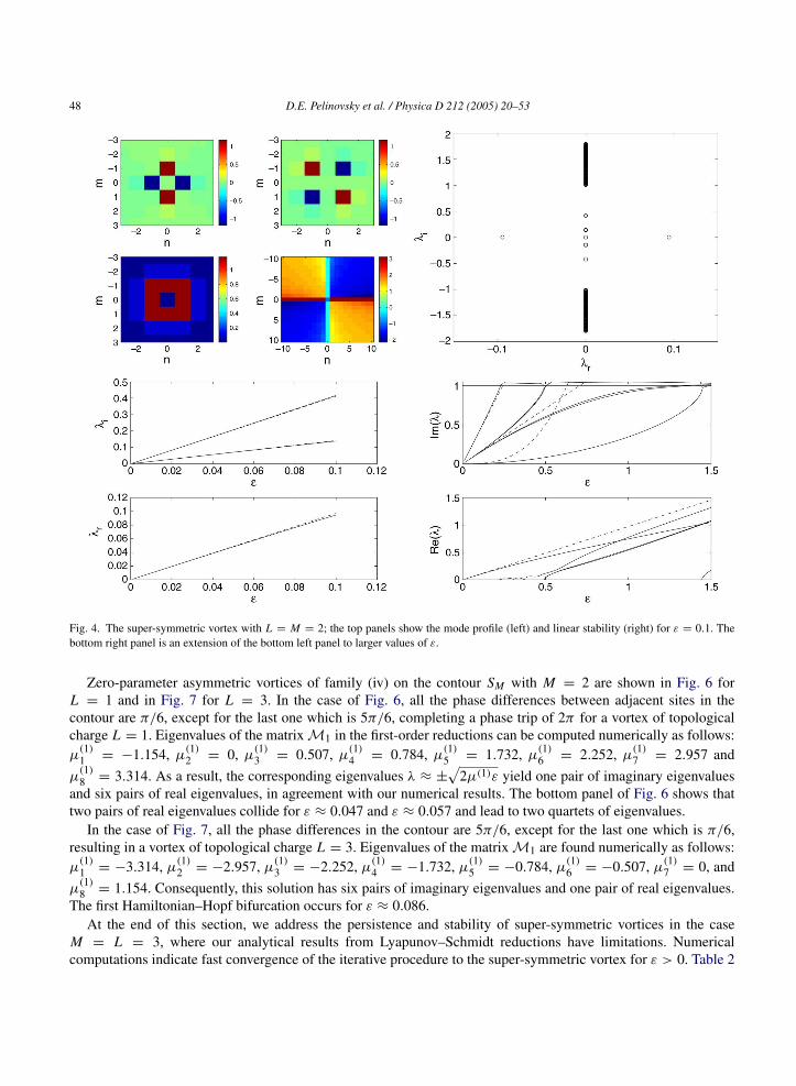
48 D.E. Pelinovsky et al. / Physica D 212 (2005) 20–53
Fig. 4. The super-symmetric vortex with L = M = 2; the top panels show the mode profile (left) and linear stability (right) for ε = 0.1. Thebottom right panel is an extension of the bottom left panel to larger values of ε.
Zero-parameter asymmetric vortices of family (iv) on the contour SM with M = 2 are shown in Fig. 6 forL = 1 and in Fig. 7 for L = 3. In the case of Fig. 6, all the phase differences between adjacent sites in thecontour are π/6, except for the last one which is 5π/6, completing a phase trip of 2π for a vortex of topologicalcharge L = 1. Eigenvalues of the matrixM1 in the first-order reductions can be computed numerically as follows:µ
(1)1 = −1.154, µ
(1)2 = 0, µ
(1)3 = 0.507, µ
(1)4 = 0.784, µ
(1)5 = 1.732, µ
(1)6 = 2.252, µ
(1)7 = 2.957 and
µ(1)8 = 3.314. As a result, the corresponding eigenvalues λ ≈ ±
√2µ(1)ε yield one pair of imaginary eigenvalues
and six pairs of real eigenvalues, in agreement with our numerical results. The bottom panel of Fig. 6 shows thattwo pairs of real eigenvalues collide for ε ≈ 0.047 and ε ≈ 0.057 and lead to two quartets of eigenvalues.
In the case of Fig. 7, all the phase differences in the contour are 5π/6, except for the last one which is π/6,resulting in a vortex of topological charge L = 3. Eigenvalues of the matrixM1 are found numerically as follows:µ
(1)1 = −3.314, µ
(1)2 = −2.957, µ
(1)3 = −2.252, µ
(1)4 = −1.732, µ
(1)5 = −0.784, µ
(1)6 = −0.507, µ
(1)7 = 0, and
µ(1)8 = 1.154. Consequently, this solution has six pairs of imaginary eigenvalues and one pair of real eigenvalues.
The first Hamiltonian–Hopf bifurcation occurs for ε ≈ 0.086.At the end of this section, we address the persistence and stability of super-symmetric vortices in the case
M = L = 3, where our analytical results from Lyapunov–Schmidt reductions have limitations. Numericalcomputations indicate fast convergence of the iterative procedure to the super-symmetric vortex for ε > 0. Table 2
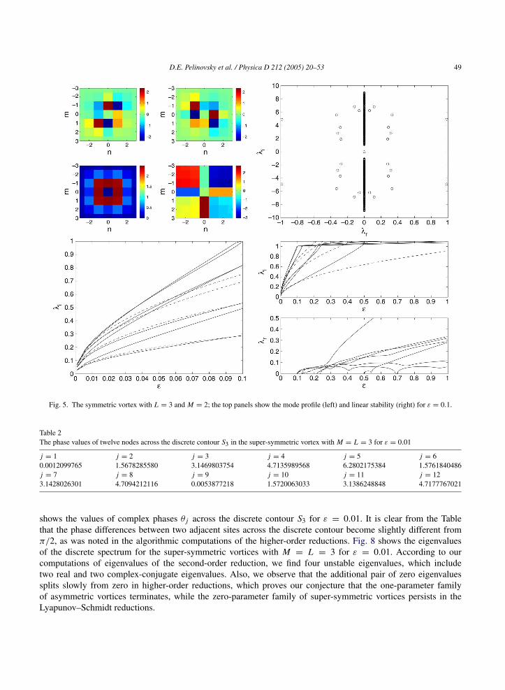
D.E. Pelinovsky et al. / Physica D 212 (2005) 20–53 49
Fig. 5. The symmetric vortex with L = 3 and M = 2; the top panels show the mode profile (left) and linear stability (right) for ε = 0.1.
Table 2The phase values of twelve nodes across the discrete contour S3 in the super-symmetric vortex with M = L = 3 for ε = 0.01
j = 1 j = 2 j = 3 j = 4 j = 5 j = 60.0012099765 1.5678285580 3.1469803754 4.7135989568 6.2802175384 1.5761840486j = 7 j = 8 j = 9 j = 10 j = 11 j = 123.1428026301 4.7094212116 0.0053877218 1.5720063033 3.1386248848 4.7177767021
shows the values of complex phases θ j across the discrete contour S3 for ε = 0.01. It is clear from the Tablethat the phase differences between two adjacent sites across the discrete contour become slightly different fromπ/2, as was noted in the algorithmic computations of the higher-order reductions. Fig. 8 shows the eigenvaluesof the discrete spectrum for the super-symmetric vortices with M = L = 3 for ε = 0.01. According to ourcomputations of eigenvalues of the second-order reduction, we find four unstable eigenvalues, which includetwo real and two complex-conjugate eigenvalues. Also, we observe that the additional pair of zero eigenvaluessplits slowly from zero in higher-order reductions, which proves our conjecture that the one-parameter familyof asymmetric vortices terminates, while the zero-parameter family of super-symmetric vortices persists in theLyapunov–Schmidt reductions.

50 D.E. Pelinovsky et al. / Physica D 212 (2005) 20–53
Fig. 6. The asymmetric vortex with L = 1 and M = 2; the top panels show the mode profile (left) and linear stability (right) for ε = 0.1.
6. Conclusion
In the present work we have developed the mathematical analysis of discrete soliton and vortex solutions ofthe two-dimensional NLS lattice with small coupling between lattice nodes. These solutions are relevant to recentexperimental and numerical studies in the context of nonlinear optics, photonic crystal lattices, soft condensed-matter physics, and Bose–Einstein condensates.
We have examined the persistence of discrete vortices starting from the anti-continuum limit of uncoupledoscillators and continuing towards a finite coupling constant ε. We have found persistent families of such solutionsthat include symmetric and asymmetric vortices. We have ruled out other non-persistent solutions by means ofthe Lyapunov–Schmidt reduction method. For persistent solutions, we have derived the leading-order asymptoticapproximations for small unstable and neutrally stable eigenvalues of the stability problem.
We have applied the results to particular computations of discrete vortices of topological charge L = 1, L = 2,and L = 3 on the discrete square contours SM with M = 1, M = 2, and M = 3. Besides particular computationscollected in Table 1 and Figs. 2–7, these results offer a road map for stability predictions for larger contours,as well as predictions on how to stabilize the discrete vortices. For example, super-symmetric vortices of chargeL = M ≥ 2 can be stabilized by excluding the inner nodes inside the discrete contour SM .

D.E. Pelinovsky et al. / Physica D 212 (2005) 20–53 51
Fig. 7. The asymmetric vortex with L = 3 and M = 2; the top panels show the mode profile (left) and linear stability (right) for ε = 0.1.
Fig. 8. Eigenvalues of the super-symmetric vortex with L = 3 and M = 3 for ε = 0.01.
52 D.E. Pelinovsky et al. / Physica D 212 (2005) 20–53
There are remaining open problems for future analytical work. First, it would be nice to extend this analysisto three-dimensional structures, such as the discrete solitons, vortices, or vortex “cubes” (see [26–28]). Second,other types of contours can be studied in the two-dimensional lattice, such as the diagonal square contourswhich would include the “vortex cross” or the octagon (see [25]). While, conceptually, the methodologies andtechniques presented here can be adapted to the problems mentioned above, actual computations of the higher-order Lyapunov–Schmidt reductions become technically involved but can be carried out with symbolic computingsoftware.
Acknowledgements
One of the authors (DEP) thanks R. Kollar and A. Scheel for useful discussions of results of this paper. This workwas partially supported by the NSERC and PREA grants for DEP and by the NSF-DMS-0204585, NSF-CAREER,NSF-DMS-0505663 and the Eppley Foundation for Research for PGK.
References
[1] D.E. Pelinovsky, P.G. Kevrekidis, D.J. Frantzeskakis, Stability of discrete solitons in nonlinear Schrodinger equations, Phys. D (2005)Preprint: nlin/0410005. doi:10.1016/j.physd.2005.07.021.
[2] S. Aubry, Breathers in nonlinear lattices: existence, linear stability and quantization, Phys. D 103 (1997) 201–250.[3] S. Flach, C.R. Willis, Discrete breathers, Phys. Rep. 295 (1998) 181–264.[4] D. Hennig, G. Tsironis, Wave transmission in nonlinear lattices, Phys. Rep. 307 (1999) 333–432.[5] P.G. Kevrekidis, K.O. Rasmussen, A.R. Bishop, The discrete nonlinear Schrodinger equation: A survey of recent results, Int. J. Mod. Phys.
B 15 (2001) 2833.[6] V.V. Konotop, V.A. Brazhnyi, Theory of nonlinear matter waves in optical lattices, Mod. Phys. Lett. B 18 (2004) 627–651.[7] P.G. Kevrekidis, D.J. Frantzeskakis, Pattern forming dynamical instabilities of Bose–Einstein condensates, Mod. Phys. Lett. B 18 (2004)
173–202.[8] M. Johansson, S. Aubry, Yu.B. Gaididei, P.L. Christiansen, K.O. Rasmussen, Dynamics of breathers in discrete nonlinear Schrodinger
models, Phys. D 119 (1998) 115–124.[9] B.A. Malomed, P.G. Kevrekidis, Discrete vortex solitons, Phys. Rev. E 64 (2001) 026601.
[10] T. Cretegny, S. Aubry, Spatially inhomogeneous time-periodic propagating waves in anharmonic systems, Phys. Rev. B 55 (1997)R11929–R11932.
[11] T. Cretegny, S. Aubry, Patterns of energy flux in periodic solutions of Klein–Gordon lattices, Phys. D 113 (1998) 162–165.[12] N.K. Efremidis, S. Sears, D.N. Christodoulides, J.W. Fleischer, M. Segev, Discrete solitons in photorefractive optically induced photonic
lattices, Phys. Rev. E 66 (2002) 046602.[13] A.A. Sukhorukov, Yu.S. Kivshar, H.S. Eisenberg, Y. Silberberg, Spatial optical solitons in waveguide arrays, IEEE J. Quantum Electron.
39 (2003) 31–50.[14] F.S. Cataliotti, S. Burger, C. Fort, P. Maddaloni, F. Minardi, A. Trombettoni, A. Smerzi, M. Inguscio, Josephson junction arrays with
Bose–Einstein condensates, Science 293 (2001) 843–846.[15] F.S. Cataliotti, L. Fallani, F Ferlaino, C. Fort, P. Maddaloni, M. Inguscio, Superfluid current disruption in a chain of weakly coupled
Bose–Einstein condensates, New J. Phys. 5 (2003) 71.[16] J.W. Fleischer, T. Carmon, M. Segev, N.K. Efremidis, D.N. Christodoulides, Observation of discrete solitons in optically induced real
time waveguide arrays, Phys. Rev. Lett. 90 (2003) 023902.[17] H. Martin, E.D. Eugenieva, Z. Chen, D.N. Christodoulides, Discrete solitons and soliton-induced dislocations in partially coherent
photonic lattices, Phys. Rev. Lett. 92 (2004) 123902.[18] J. Yang, I. Makasyuk, A. Bezryadina, Z. Chen, Dipole solitons in optically induced two-dimensional photonic lattices, Opt. Lett. 29 (2004)
1662–1664.[19] Z. Chen, H. Martin, E.D. Eugenieva, J. Xu, A. Bezryadina, Anisotropic enhancement of discrete diffraction and formation of two-
dimensional discrete-soliton trains, Phys. Rev. Lett. 92 (2004) 143902.[20] Z. Chen, A. Bezryadina, I. Makasyuk, J. Yang, Observation of two-dimensional lattice vector solitons, Opt. Lett. 29 (2004) 1656–1658.[21] D.N. Neshev, T.J. Alexander, E.A. Ostrovskaya, Yu.S. Kivshar, H. Martin, I. Makasyuk, Z. Chen, Observation of discrete vortex solitons
in optically induced photonic lattices, Phys. Rev. Lett. 92 (2004) 123903.[22] J.W. Fleischer, G. Bartal, O. Cohen, O. Manela, M. Segev, J. Hudock, D.N. Christodoulides, Observation of vortex-ring discrete solitons
in 2D photonic lattices, Phys. Rev. Lett. 92 (2004) 123904.

D.E. Pelinovsky et al. / Physica D 212 (2005) 20–53 53
[23] J. Yang, Z. Musslimani, Fundamental and vortex solitons in a two-dimensional optical lattice, Opt. Lett. 28 (2003) 2094–2096.[24] P.G. Kevrekidis, B.A. Malomed, Z. Chen, D.J. Frantzeskakis, Stable higher-order vortices and quasi-vortices in the discrete nonlinear
Schrodinger equation, Phys. Rev. E 70 (2004) 056612.[25] J. Yang, I. Makasyuk, P.G. Kevrekidis, H. Martin, B.A. Malomed, D.J. Frantzeskakis, Z. Chen, Necklace-like solitons in optically induced
photonic lattices, Phys. Rev. Lett. 94 (2005) 113902.[26] P.G. Kevrekidis, B.A. Malomed, D.J. Frantzeskakis, R. Carretero-Gonzalez, Three-dimensional solitary waves and vortices in a discrete
nonlinear Schrodinger lattice, Phys. Rev. Lett. 93 (2004) 080403.[27] R. Carretero-Gonzalez, P.G. Kevrekidis, B.A. Malomed, D.J. Frantzeskakis, Three-dimensional nonlinear lattices: from oblique vortices
and octupoles to discrete diamonds and vortex cubes, Phys. Rev. Lett. 94 (2005) 203901.[28] T.J. Alexander, E.A. Ostrovskaya, A.A. Sukhorukov, Yu.S. Kivshar, Three-dimensional matter-wave vortices in optical lattices. cond-
mat/0501590.[29] T.J. Alexander, A.A. Sukhorukov, Yu.S. Kivshar, Asymmetric vortex solitons in nonlinear periodic lattices, Phys. Rev. Lett. 93 (2004)
063901.[30] M. Johansson, S. Aubry, Existence and stability of quasiperiodic breathers in the discrete nonlinear Schrodinger equation, Nonlinearity
10 (1997) 1151–1178.[31] R.S. MacKay, Slow manifolds, in: T. Dauxois, A. Litvak-Hinenzon, R.S. MacKay, A. Spanoudaki (Eds.), Energy Localization and
Transfer, World Scientific, Singapore, 2004, pp. 149–192.[32] R.S. MacKay, S. Aubry, Proof of existence of breathers for time-reversible or Hamiltonian networks of weakly coupled oscillators,
Nonlinearity 7 (1994) 1623–1643.[33] V. Koukouloyannis, R.S. MacKay, Existence and stability of 3-site breathers in a triangular lattice, J. Phys. A: Math. Gen. 38 (2005)
1021–1030.[34] S.N. Chow, J.K. Hale, Methods of Bifurcation Theory, Springer Verlag, 1982.[35] M. Golubitsky, D.G. Schaeffer, Singularities and Groups in Bifurcation Theory, vol. 1, Springer Verlag, New York, 1985.[36] T. Kapitula, P.G. Kevrekidis, Linear stability of perturbed Hamiltonian systems: theory and a case example, J. Phys. A: Math. Gen. 37
(2004) 7509–7526.[37] B. Sandstede, Stability of multiple-pulse solutions, Trans. Amer. Math. Soc. 350 (1998) 429–472.[38] H. Levy, F. Lessman, Finite Difference Equations, Dover, New York, 1992.[39] V. Vougalter, D. Pelinovsky, Eigenvalues of zero energy in the linearized NLS problem, 2005 (preprint).