Is there persistence in innovative activities

International Journal of Industrial Organization21 (2003) 489–515

www.elsevier.com/ locate/econbase

I s there persistence in innovative activities?

*Elena CefisDepartment of Economics, University of Bergamo, via dei Caniana 2, 24127Bergamo, Italy

Received 10 February 2001; received in revised form 21 November 2001; accepted 5 June 2002

Abstract

This paper examines firm innovative persistence using patent applications of 577 UKmanufacturing firms. Non-parametric techniques show the empirical distributions of patentsare neither Geometric nor Poisson. There exists a threshold effect represented by the firstpatent: the probability to go from zero to one patent is uniformly much lower than fromn ton 1 1 patents, withn >1. Transition Probability Matrices show little persistence in general,but strong persistence among ‘great’ innovators that account for a large proportion ofpatents requested: innovative activities, at least which are captured by patents, arepersistent. There is heterogeneity across industrial and size classification. 2002 Elsevier Science B.V. All rights reserved.

JEL classification: L20; L60; O31; D21

Keywords: Innovation; Patents; Persistence; Transition probability matrices

1 . Introduction

The purpose of this paper is to analyse patent time series as a proxy forinnovative activities at firm level. The focus in particular is upon the dynamicfeatures of the patent time series. Pertinent questions concern whether oneobserves e.g. convergence to the mean, persistence or explosive paths.

*Tel.: 139-035-2052-547; fax:139-035-277-549.E-mail address: [email protected](E. Cefis).

0167-7187/02/$ – see front matter 2002 Elsevier Science B.V. All rights reserved.doi:10.1016/S0167-7187(02)00090-5

mailto:[email protected]

490 E. Cefis / Int. J. Ind. Organ. 21 (2003) 489–515

These issues have implications for patterns of firms’ growth, the nature ofinnovative activities, and industrial dynamics.

An important stylised fact concerning the dynamics of firms’ growth is thatfirms display persistent differences (Dosi et al., 1995; Coriat and Dosi, 1998,Bottazzi et al., 2001, 2002). These differences (or asymmetries) pertain toproductivity and costs (Nelson and Winter, 1982; Baily and Chakrabarty, 1985), toprofitability (Mueller, 1990; Geroski et al., 1993), and to innovative output(Griliches, 1986; Patel and Pavitt, 1991). What is particularly intriguing is thepersistence of these asymmetries, so that for example, firms enjoying higher(lower) profits can be expected to earn higher (lower) profits also in the future: that

1is to say, profits do not seem to converge to a common rate of return . Persistentasymmetries among firms involve interesting questions, such as what their sourcesare, why competitive interactions do not make them vanish, and what theirconsequences are for industrial dynamics. Since technological innovation is one ofthe ‘driving forces’ of firms’ growth, and, at the same time, there are differencesamong firms in innovative output, it is of particular interest to ask whether data oninnovative activities at the firm level show persistence across firms.

The issue of persistence in innovative activities is particularly relevant in thecontext of the discussion about the properties of the patterns of innovativeactivities. Since Schumpeter, the economic literature on technological change hasdeveloped two main views of the innovation process. Referring to what Schumpe-ter states inThe Theory of Economic Development (1934) (known as theSchumpeter Mark I model) the process of technological change is considered aprocess of ‘creative destruction’. Conversely, referring to the Schumpeter ofCapitalism, Socialism,and Democracy (1942) the process is seen as a process of‘creative accumulation’ (or Schumpeter Mark II model). The difference betweenthe two depends on fundamental assumptions about the properties of technology

2and of the innovative process .In a rather simplified way, in Schumpeter Mark I technology is equally

accessible to everybody and technological change is a random process, driven by a

1Substantial research effort has been devoted to the examination of profit persistence. Recentliterature has addressed the following question: do industrial profits rates eventually converge to acommon rate? Several empirical studies have shown that firms display persistent differences inprofitability (Mueller, 1990; Geroski and Jacquemin, 1988). That is, profits do not seem to converge toa common rate of return. Moreover, evidence seems to indicate that the adjustment of profits to theirfirm-specific ‘permanent’ values is rather quick, although a significant variability is observed acrossdifferent countries (see for example, Odagiri and Yamawaki, 1990; Cubbin and Geroski, 1987).However, it is hard to say to what extent the observed persistence in profitability differentials reflectsthe persistence of differential ‘efficiency’ levels which are not eroded away by the competitive process.Only very recently has it been tried to link the strong inertia of firm profits and the persistence ininnovation activities (Cefis, 2001).

2See Dosi (1988), Martin (2001, ch. 14) and Winter (1984).

E. Cefis / Int. J. Ind. Organ. 21 (2003) 489–515 491

population of homogeneous firms who have a certain probability of realizingtechnological opportunities. Innovation generates monopoly power that is at bestonly temporary, since it is quickly challenged and eroded by competitors. Sincethe relevant knowledge base is easily available, new innovators systematicallysubstitute for incumbents and typical innovators are small, newly established firms.

Conversely, in Schumpeter Mark II technical knowledge has a strong tacitcomponent and is highly specific to individual firms. Innovation results from theaccumulation of technological competencies by heterogeneous firms. Firm-specifictechnical change is cumulative, meaning that the generation of new knowledgebuilds upon what has been learned in the past and accumulated competenciessignificantly constrain the future technological performance of the firm. Over time,the firm-specific, tacit, and cumulative nature of the knowledge base builds highbarriers to entry. A few (large) firms eventually come to dominate the market in astable oligopoly.

Thus, the presence or absence of persistence in innovative activities is a majorproperty of the innovative process and an important feature of the patterns of

3technological change, which has significant implications for both theory andpolicy-making.

Because of its cumulative nature, technological change is usually characterisedby dynamic increasing returns (learning-by-doing, learning-to-learn, researchbreeds new opportunities, etc.). Persistence in innovative activities might meanthat technological change could be one source of increasing returns that cansupport persistent growth (Barro and Sala-i-Martin, 1995).

Persistence, in general, would give some support to the ‘competence-based’theory of the firm at the microeconomic level (Nelson and Winter, 1982; Teeceand Pisano, 1994), as well as to endogenous growth theories at the macroeconomiclevel. On the contrary, persistence in innovative activities would weaken thoseinterpretations of the processes of growth of firms, industries and countries(ranging from simple Gibrat-type processes to the models of the real businesscycle) where dynamics is essentially driven by small uncorrelated shocks. Moregenerally, understanding whether innovative activities are persistent or not at thefirm level would constitute an important piece of evidence for founding andimproving current theories of industrial dynamics and evolution, where someforms of dynamic increasing returns play a major role in determining degrees ofconcentration and its stability over time, rates of entry and exit and so forth(Klepper, 1996; Jovanovic, 1982; Hopenhayn, 1992; Nelson and Winter, 1982;Dosi et al., 1995).

3Models as different in inspiration as those of Nelson and Winter (1982) and Ericson and Pakes(1992) show that these two alternative patterns of technological change can be interpreted as two facesof the stochastic process which drives technological accumulation at the firm level and thereby drivesthe dynamics of the industry.


However, very little is known about the relative empirical relevance ofpersistence in innovative activities. Recently, a few studies have begun to providesome (and somewhat contrasting) empirical results. Malerba and Orsenigo (1999),examining the patterns of innovative dynamics, find thatoccasional innovators(firms who patent just once) constitute a large part of the whole population ofinnovators but a much lower share of the total number of patents at any giventime. Furthermore, large innovators (both in terms of patents and employees) tendto remain large over time and constitute a relatively stable core that persistentlygenerates innovative activities, accounting for a very large share of total patents.Conversely, Geroski et al. (1997) estimate a Proportional Hazards Model of theprobability that the spell of time in which a firm innovates will end at anyparticular moment. They find little evidence of persistence at the firm level. Veryfew firms innovate persistently and this happens only after a threshold level (5patents or 3 major innovations) which only a few firms ever reach.

In the present study I analyse the persistence properties of patent data, using anon-parametric approach based on Transition Probabilities Matrices (TPMs). Thedata set is composed of patents requested from the European Patent Office by arandom sample of 577 UK manufacturing firms during the period 1978–1991.Examining the properties of the empirical distributions of patents, I found thatpatent distributions are not geometric. They do not display the lack-of-memoryproperty and exhibit negative duration dependence. There appears to exist athreshold effect represented by the first patent every year in the sample. It is muchmore difficult to apply for the first patent than to go fromn to n 1 1 patents, withn > 1.

The transition probabilities across states suggest that in general there is littlepersistence in innovative activities, but at the same time there is evidence of‘bimodality’ in the estimated TPMs, especially as the transition period is longer. Inother words, there is a strong persistence in remaining in the polar states, namelyin the state in which firms do not apply for a patent every year or in the state inwhich firms apply for many patents (at least 6). The ‘great’ innovators (firms thatapply for at least six patents per year) are very few in number (2.37% on average),but they account for the large majority of patents requested (77.85% on average).These results suggest that innovative activities, at least those that are captured bypatents, are persistent.

Finally, there is evidence of heterogeneity across the dimensions of the sample,industrial and size classification. The mechanical engineering sector shows lowpersistence and low bimodality, while the chemical industry shows high per-sistence and high bimodality, implying that innovative activities are sector specific.Large firms show more persistence than small firms, in line with the SchumpeterMark II hypothesis.

The rest of the paper is organised as follows: the next section describes the data,while Section 3 describes the methodologies used to analyse the data. Section 4presents the results and Section 5 the sensitivity analysis. Conclusions follow.


2 . The data

The data set of this study is a time-series of patents requested by 577 U.K.manufacturing firms during the period 1978–1991. The random sample of firmswas chosen from the population of 6052 U.K. firms that from 1978 to 1991 have

4 5applied for at least one patent to the European Patent Office .In addition, for the year 1991, there are variables concerning firm size, industrial

classification and other firm characteristics (quoted vs. non-quoted, independentvs. subsidiary). The number of employees was chosen as a proxy for size.According to the number of employees in 1991, firms were divided in four sizegroups: small (from 1 to 99 employees), medium (100–499), medium-large firms(500–999), and large (at least 1000 employees).

Firms were grouped according to two-digit industrial classification althoughinformation at four-digit level for each firm was available (provided by ICC andDatastream), mainly because firms are usually very diversified at four-digit level

6(and it is very difficult to assign a firm to a particular four-digit industry ), and,secondly, because to undertake a meaningful empirical analysis it is necessary tohave sub-groups with a sufficient number of observations. Because of these dataconstraints, only four sectors were analysed (namely, chemical, 69 firms; me-chanical engineering, 132; electrical and electronic machinery, 100; and instrumentengineering, 56).

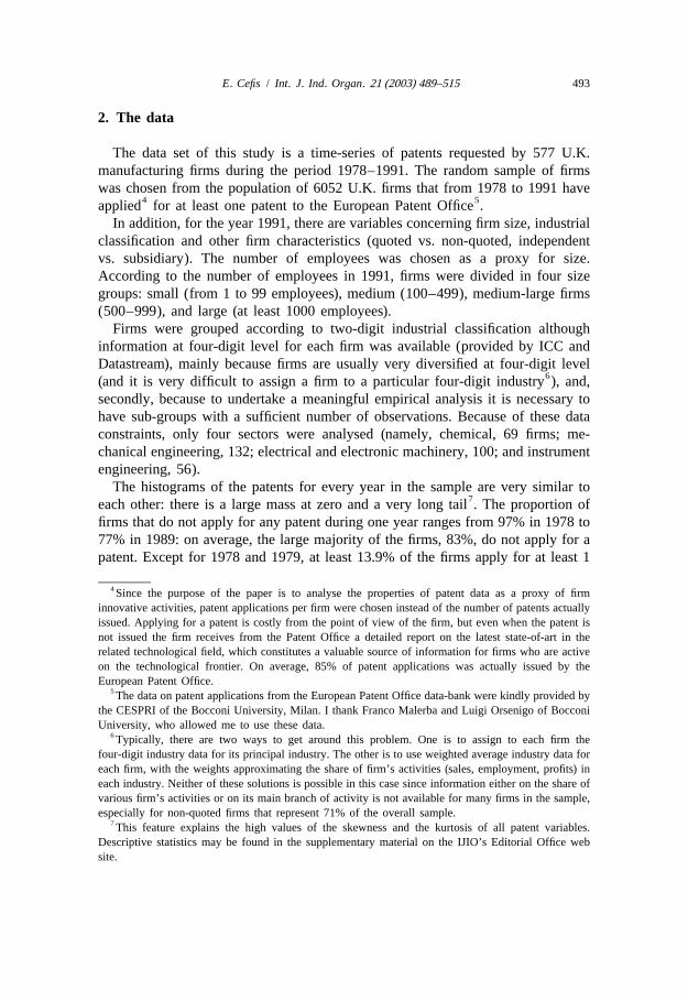
The histograms of the patents for every year in the sample are very similar to7each other: there is a large mass at zero and a very long tail . The proportion of

firms that do not apply for any patent during one year ranges from 97% in 1978 to77% in 1989: on average, the large majority of the firms, 83%, do not apply for apatent. Except for 1978 and 1979, at least 13.9% of the firms apply for at least 1

4Since the purpose of the paper is to analyse the properties of patent data as a proxy of firminnovative activities, patent applications per firm were chosen instead of the number of patents actuallyissued. Applying for a patent is costly from the point of view of the firm, but even when the patent isnot issued the firm receives from the Patent Office a detailed report on the latest state-of-art in therelated technological field, which constitutes a valuable source of information for firms who are activeon the technological frontier. On average, 85% of patent applications was actually issued by theEuropean Patent Office.

5The data on patent applications from the European Patent Office data-bank were kindly provided bythe CESPRI of the Bocconi University, Milan. I thank Franco Malerba and Luigi Orsenigo of BocconiUniversity, who allowed me to use these data.

6Typically, there are two ways to get around this problem. One is to assign to each firm thefour-digit industry data for its principal industry. The other is to use weighted average industry data foreach firm, with the weights approximating the share of firm’s activities (sales, employment, profits) ineach industry. Neither of these solutions is possible in this case since information either on the share ofvarious firm’s activities or on its main branch of activity is not available for many firms in the sample,especially for non-quoted firms that represent 71% of the overall sample.

7This feature explains the high values of the skewness and the kurtosis of all patent variables.Descriptive statistics may be found in the supplementary material on the IJIO’s Editorial Office website.


patent per year; while if I include 1978 and 1979 I obtain that, on average, 10%apply for a patent and 6% apply for more than one patent per year.

The frequency distribution of total patents requested over the entire period1978–1991 shows that 53% of the firms request only one patent over the entireperiod, 16% two patents and 15% apply for between half a dozen and two hundredpatents. The figure that clearly emerges from this data is that about half of thefirms who patent, did so only once, while 16% produce at least one patent per yearon average.

Reorganising the data according to firm characteristics provides interestingadditional evidence. On average, 17.5% of quoted firms apply for at least 1 patentevery year, compared with only 9% of the non-quoted firms. The differencebetween the two averages is statistically significant, while the difference betweenthe same averages for the independent firms (25%) and the subsidiaries firms(24%) is not significant. While it matters that a firm is quoted or non-quoted, itmakes no difference with respect to the ‘production’ of patents that it isindependent or subsidiary. Indeed, the subsidiary sub-group includes researchlaboratories of large business firms/groups (when they are an autonomous firm)that apply for many patents per year.

The distribution of patents by industry is very stable over time. On average,25% of the firms in chemical industry have at least 1 patent per year, 16.6% inmechanical engineering, 17% in electrical and electronic machinery, and slightlyabove 20% in instrument engineering. Cumulatively, 23% of firms have at least 6patents in chemical industry, 14% in mechanical engineering, 15% in electricaland electronic machinery, and 18% in instrument engineering. The data show thatthe chemical industry has the highest propensity to patent, although to put thesenumbers into a correct perspective we have to keep in mind that these are the fourmajor innovative sectors of the industry classification.

3 . Methodology

3 .1. The distributional properties of patent data

To analyse the distributional properties of patent data I examined the empiricaldistributions of patents for every year in the sample. In particular, I am interestedin testing whether these distributions are geometric or Poisson. If patent dis-tributions are geometric, they will display ‘lack of memory’ and aconstant hazardrate, while if they are Poisson it means that the patenting process is random with agiven intensity (or mean capacity) to patent that cannot certainly be cumulative orpath-dependent.

In order to test these hypotheses, I assume that the individual variables, thenumber of patents requested each year by a firm, are independent, which is astrong assumption to make in view of the rest of the analysis. To partially


overcome this limitation, I perform the same tests on the distribution of thecumulative sum of patents for every firm over the 14 years of the sample.

3 .2. Persistence properties

I measure persistence as a firm’s probability of remaining in its initial state.Namely, if a firm is asystematic innovator (that is, applies for at least one patentin a year) I am interested in knowing what is the probability that it remains a

8systematic innovator as time passes .To investigate whether patents data show some persistence, one could simply

model the data for each firm as an autoregressive model and estimate thepersistence parameter by standard econometric tools. However, given the shortnessof the patents time series, standard OLS regression tools give a biased estimate ofthe true persistence parameter in small samples. One needs to exploit both thecross sectional and the time series information of the sample. An econometricstrategy suggested by Quah (1993a,b) deals with the dynamics and cross-sectiondimensions, based on what is called Random Fields. At each point in time there isa cross-section distribution of firms’ patents, which is the realisation of a randomelement in the space of distributions. The idea is to describe their evolution overtime, which will allow us to analyse intra-distribution mobility and persistence ofthe firms’ innovative activities.

In the context of Random Fields, the realisation of a random element is across-section distribution function that can be estimated from the data (Silverman,1986, Section 2.10). However, there are two limitations of the distributionfunctions in this context. One is that persistence is generally a dynamic conceptwhile the cross-section distributions are point-in-time estimates, available for1978–1991. Further, the distribution functions do not give any information aboutthe firm’s relative situation and its movement over time. To deal with theselimitations, it is necessary to derive a law of motion for the cross-sectiondistributions in a more formal structure.

Let F denote the distribution of patents across firms at timet; and let ust

describehF : integer tj’s evolution by the law of motion:t

F 5P ?F (1)t11 t

whereP maps one distribution into another, and tracks where points inF end upt

in F . Eq. (1) is analogous to a standard first-order autoregression, except that itst11

8 It is worth emphasising that defining as ‘innovators’ firms that applied at least once for a patent inthe period of observation, our sample is constituted only by innovating firms. The purpose of the paperis to detect whether the firms that innovate do so persistently. Therefore, problems of endogenoussample selection do not arise because properties of the total population of firms are not inferred fromthis sample but only properties of the sub-group of innovating firms.


values are distributions (rather than scalars or vectors of numbers), and it containsno explicit disturbance or innovation. By analogy with autoregression, there is noreason why the law of motion forF need be first-order, or why the relation needt

be time-invariant. Nevertheless, (1) is a useful first step for analysing the dynamicsof hF j, and afterwards I will drop these assumptions and test the robustness of thet

results to these hypotheses. OperatorP of (1) can be approximated by assuming a9finite state space for firmsS 5 hs , s , . . . , s j, where s (i 5 1, . . . , r) are the1 2 r i

possible states. In this caseP is simply a Transition Probability Matrix (TPM).Pencodes the relevant information about mobility and persistence within the crosssection distributions.

Therefore, assuming that the law of motion forF is time-invariant and oft

first-order, the one-step transition probability is defined by:

p 5P(X 5 juX 5 i) (2)ij t1n t

with t51978, 1979,. . . , 1993 andn51, 5, 10 years.The TPM P is the matrix with p as elements measuring the probability ofij

moving from statei to statej in one period.This TPM offers useful information for analysing persistence since it measures

the probability that a firm goes from a state to another state in one period. A stateis identified by the number of patent applications filed each year.

TPMs can be computed on the percentiles of the empirical distribution or onarbitrary bounds selected by the user. The focal attention of the analysis is on thetransition of firms from the state in which they do not apply for a patent in a givenyear to the state in which they apply for at least one patent in the subsequent year.Within this latter state, the attention focuses on the transitions between states inwhich firms applied for a low, medium or great number of patents.

Subsequently, two and four state TPMs are computed. In the first TPM, i.e. thetwo states, the first state is defined as having requested no patents at all in a year(what it is called the ‘occasional innovator’ state), while the second one representshaving requested at least one patent (the ‘systematic innovator’ state). In thefour-state TPM, the states were selected as follows, first state (occasionalinnovator): having requested no patents at all; second state (small innovator):having requested 1 patent; third state (medium innovator): having requested from 2to 5 patents; fourth state (great innovator): having requested at least six patents.

Once TPMs have been obtained, the first-order autoregressive parameter implied

9Suppose a moving particle and denote its range byI. This may be a finite or infinite set of integersand it may be an arbitrary countable set of elements, provided that the definition of random variables isextended to take values in such a set. Let us callI the state space and an element of it a state. Theparticle moves from state to state. There is a set of transition probabilitiesp , where, such that: if theij

particle is in the statei at any time the probability that it will be in the statej after one step is given byp .ij


by each chain is calculated, as suggested in Amemiya (1994). This will be used asa synthetic measure of persistence in innovative activities.

Let x be a stochastic process approximated by a two-state Markov chain witht

transition probabilities:

p 12 pP[X 5 juX 5 i] 5 . (3)F Gt t21 12 q q

The implied AR(1) process forx can be constructed as:t

x 5 (12 q )1r x 1 v , (4)t 1 1 t21 t

wherer 5 p 1 q 2 1.According to our definition, there is persistence in innovative activities ifr is

greater than 0. This certainly happens when both the diagonal elements of theTPM are larger than 0.5. When the elements of the main diagonal are all equal to1, there is perfect persistence. Conversely, ifp and q are both smaller than 0.5,r,0, that is, there is a tendency to revert from one state to the other in everyperiod, and the innovative activities could be characterised as non-persistent.

TPMs are computed for three different period lengths: (i) 1 year; (ii) 5 years tocapture medium run dynamics; (iii) 10 years to illustrate the long run dynamics.Therefore, three different first-order autoregressive parametersr , r , andr are1 5 10

calculated which measure persistence in the following AR(1) processes:

x 5 (12 q )1r x 1 vt 1 1 t21 t

x 5 (12 q )1r x 1 vt 5 5 t25 t

x 5 (12 q )1r x 1 vt 10 10 t210 t

Once the TPMs of interest have been calculated, the resulting probabilities areestimates of the transition probabilities. Then a non-parametric approach is used toassess the accuracy of these estimates. This approach consists in applying thebootstrapping methodology to the transition matrices to find the standard errorsassociated with transition probabilities (see Cefis, 1999 for bootstrapping appliedto TPMs).

4 . Results

4 .1. Examining the distributional properties of patent data

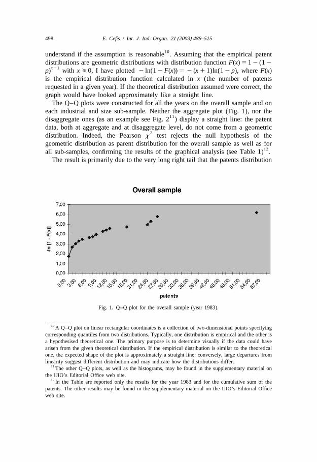
Examining the histograms of the patents for every year in the sample suggeststhat patents data could come from a geometric distribution. I use a graphicalprocedure, namely a Q–Q plot (Wilk and Gnanadesikan, 1968), in order to


10understand if the assumption is reasonable . Assuming that the empirical patentdistributions are geometric distributions with distribution functionF(x)5 12 (12

x11p) with x > 0, I have plotted2 ln(12F(x))5 2 (x 1 1)ln(12 p), whereF(x)is the empirical distribution function calculated inx (the number of patentsrequested in a given year). If the theoretical distribution assumed were correct, thegraph would have looked approximately like a straight line.

The Q–Q plots were constructed for all the years on the overall sample and oneach industrial and size sub-sample. Neither the aggregate plot (Fig. 1), nor the

11disaggregate ones (as an example see Fig. 2 ) display a straight line: the patentdata, both at aggregate and at disaggregate level, do not come from a geometric

2distribution. Indeed, the Pearsonx test rejects the null hypothesis of thegeometric distribution as parent distribution for the overall sample as well as for

12all sub-samples, confirming the results of the graphical analysis (see Table 1) .The result is primarily due to the very long right tail that the patents distribution

Fig. 1. Q–Q plot for the overall sample (year 1983).

10A Q–Q plot on linear rectangular coordinates is a collection of two-dimensional points specifyingcorresponding quantiles from two distributions. Typically, one distribution is empirical and the other isa hypothesised theoretical one. The primary purpose is to determine visually if the data could havearisen from the given theoretical distribution. If the empirical distribution is similar to the theoreticalone, the expected shape of the plot is approximately a straight line; conversely, large departures fromlinearity suggest different distribution and may indicate how the distributions differ.

11The other Q–Q plots, as well as the histograms, may be found in the supplementary material onthe IJIO’s Editorial Office web site.

12In the Table are reported only the results for the year 1983 and for the cumulative sum of thepatents. The other results may be found in the supplementary material on the IJIO’s Editorial Officeweb site.


Fig. 2. Q–Q plot for sub-samples (year 1983).


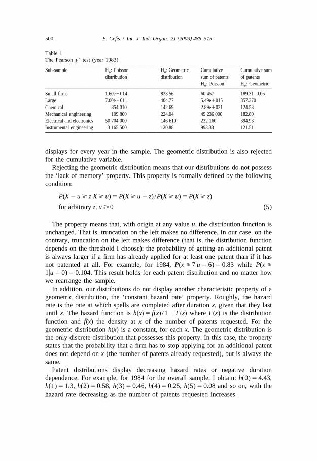
Table 12The Pearsonx test (year 1983)

Sub-sample H : Poisson H : Geometric Cumulative Cumulative sum0 0

distribution distribution sum of patents of patentsH : Poisson H : Geometric0 0

Small firms 1.60e1014 823.56 60 457 189.31–0.06Large 7.00e1011 404.77 5.49e1015 857.370Chemical 854 010 142.69 2.89e1031 124.53Mechanical engineering 109 800 224.04 49 236 000 182.80Electrical and electronics 50 704 000 146 610 232 160 394.93Instrumental engineering 3 165 500 120.88 993.33 121.51

displays for every year in the sample. The geometric distribution is also rejectedfor the cumulative variable.

Rejecting the geometric distribution means that our distributions do not possessthe ‘lack of memory’ property. This property is formally defined by the followingcondition:

P(X 2 u > zuX > u)5P(X > u 1 z) /P(X > u)5P(X > z)

for arbitraryz, u > 0 (5)

The property means that, with origin at any valueu, the distribution function isunchanged. That is, truncation on the left makes no difference. In our case, on thecontrary, truncation on the left makes difference (that is, the distribution functiondepends on the threshold I choose): the probability of getting an additional patentis always larger if a firm has already applied for at least one patent than if it hasnot patented at all. For example, for 1984,P(x > 7uu 5 6)50.83 while P(x >1uu 5 0)50.104. This result holds for each patent distribution and no matter howwe rearrange the sample.

In addition, our distributions do not display another characteristic property of ageometric distribution, the ‘constant hazard rate’ property. Roughly, the hazardrate is the rate at which spells are completed after durationx, given that they lastuntil x. The hazard function ish x 5 f(x) /12F x whereF(x) is the distributions d s dfunction andf(x) the density atx of the number of patents requested. For thegeometric distributionh(x) is a constant, for eachx. The geometric distribution isthe only discrete distribution that possesses this property. In this case, the propertystates that the probability that a firm has to stop applying for an additional patentdoes not depend onx (the number of patents already requested), but is always thesame.

Patent distributions display decreasing hazard rates or negative durationdependence. For example, for 1984 for the overall sample, I obtain:h(0)5 4.43,h(1)5 1.3, h(2)5 0.58, h(3)50.46, h(4)50.25, h(5)5 0.08 and so on, with thehazard rate decreasing as the number of patents requested increases.


For each year, the hazard rate drastically decreases fromh(0) to h(1) and thendecreases more smoothly. This feature, jointly to the fact that the probability ofgetting an additional patent is always larger if a firm has already applied for atleast one patent than if it has not patented at all, suggests that there is a thresholdto patenting, where the threshold is represented by the first patent. A firm thatpatents a lot has a higher probability of getting an additional patent than a firm thathas not patented at all. In other words, it is much more difficult to obtain the firstpatent than to go fromn to n 1 1 patents, withn > 1. These characteristics aremaintained no matter how I rearrange the samples into groups according to firms

13characteristics .Quite often in the economic literature, the patenting process is represented as a

Poisson process. The Poisson distribution is the counting distribution for thecorresponding Poisson process. The process continues over a certain index set oftime or space where specified rare events occur at random in the index with somefixed mean rate. LetX(t) be the number of occurrences of the specified events (forexample, the number of the patents requested in a year) in the time interval [0,t)with t 5 0 andX(0)50.

Usually, the standard postulates reported in the supplementary material aremade to define the Poisson process. Under the standard postulates the probabilityq (t) of exactlyx events (in our case, the probability to apply for exactlyx patents)x

x 2ltoccurring in the time interval [t, t 1 t) is q (t)5 (lt) e /x! for x 50, 1, 2, . . . .,x

which is nothing but the Poisson distribution with parameterlt, and henceX(t) iscalled the Poisson process with intensity (or mean)l (in this casel represents thepropensity, or better, the average capacity to patent).

To get the form of q (t) heuristically, the following intuitive approach isx

available. Dividing the time interval [0,t), for example a given year, intondisjoint intervals of equal lengthh 5 t /n (they can be days, working hours, etc.),then, under the postulates above, we have that the probability to get a certainnumber of patent applications,x, in a year,t, is given by a Poisson distribution. Inother words, if the patenting process is Poisson, the patent data should have aPoisson distribution.

To verify whether the empirical patent distributions are Poisson distributions, I2performed a Pearsonx test, in which the null hypothesis is that the patent data

come from a Poisson distribution. As Table 1 shows, the null hypothesis isrejected for the overall sample as well as for the industrial and size sub-samples.

Rejecting the Poisson distribution means that the postulates on which a Poissonprocess is based may not hold. In particular, if the patenting process is Poisson, it

13These results are not in contrast with those of Geroski et al. (1997). They found that there exists athreshold represented by the 5th patent or the 3rd major innovation beyond which ‘‘some form of‘dynamic scale economies’ may govern the production of patents’’. This effect is captured later in thisstudy where it is shown that estimated TPMs display strong ‘bimodality’ (see next footnote), that is‘great’ innovators tend with a very high probability to remain great innovators.


means that the process is certainly not cumulative and path-dependent, due to thestationarity (the probability of a number of events occurring in a time intervaldepends only on the number of the events and on the length of the interval, but noton time) and independence assumptions (the number of events occurring on

14non-overlapping time intervals are mutually independent ). Rejecting the Poissondistribution does not mean that the patenting process is cumulative or path-dependent, but, at least, we cannot exclude the hypothesis.

4 .2. Persistence properties

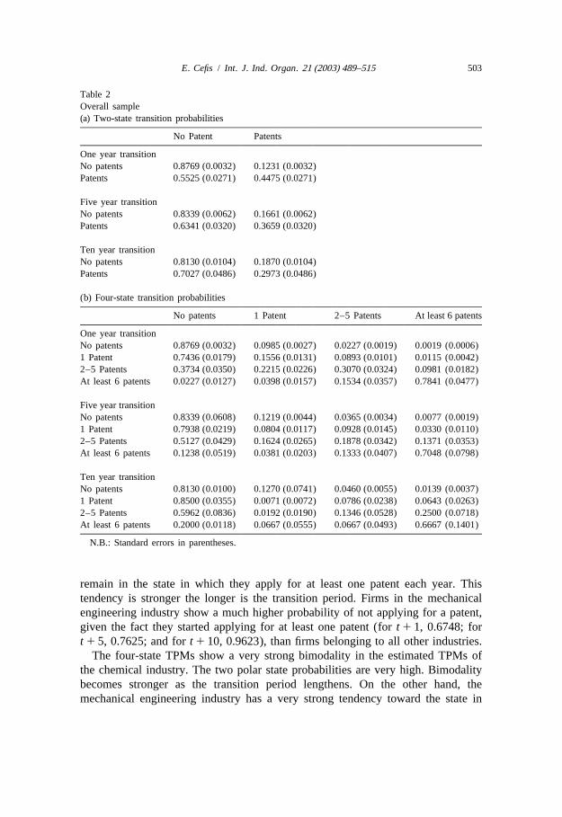
Considering first the overall sample (see Table 2), the two-state TPMs show astrong persistence of the occasional innovator state, that is, a firm which in acertain yeart has not applied for a patent, will not apply the following year (if oneyear transition periodt 1 1 is considered) for a patent with a high probability(0.8769). Besides, there is a tendency (0.5525) to reversion towards the state inwhich firms do not apply for a patent if firms started from the state of applying atleast for one patent in a year. The longer is the transition period, the stronger is thereversion. Indeed, the autoregressive coefficient goes from 0.3244 for transitionsover 1 year to 0.1103 for transitions over 10 years (see Table 7).

The four-state TPMs show that there is little persistence in general (not all thediagonal elements are substantially larger than 0.5), but there is a high probabilityof remaining in the polar states (for one year transition: 0.8769 and 0.7841), which

15with some abuse of terminology I refer to asbimodality . In other words, there isa very strong persistence in remaining in the polar states (the occasional innovatorstate and the great innovator state). Note also that over 10 year period, there is aprobability of 0.20 that a firm applying for at least 6 patents goes to the state inwhich it does not apply for a patent, while there is only a probability of 0.01 ofgoing the other way around: it is easier to lose the knowledge and organisationalcapabilities necessary to innovate than to acquire them, even in the long run.

16Concerning the firm classification by industrial sectors (Tables 3 and 4 ), thetwo-state TPMs show that in the chemical industry, and contrary to the other threesectors, there is a strong persistence of remaining in the state in which the firmstarted regardless of the length of the transition period. For the other threeindustries there is a stronger tendency to go from the state in which firms apply forat least one patent to the state in which firms do not apply for a patent, than to

14SeeThe Poisson Process — postulate number 1 and 2 in the supplementary material on the IJIO’sEditorial Office web site.

15It is worth emphasising that by the term ‘bimodality’ I am not referring to a bimodal distribution; itis only a way of saying that in a TPM the probabilities on the extreme of the main diagonal are muchhigher than the other diagonal probabilities.

16Only the results on the chemical and the mechanical sectors are reported as well as on the largeand small firms sub-samples. The other results can be found in Cefis (1999) or in the supplementarymaterial on the IJIO’s Editorial Office web site.


Table 2Overall sample(a) Two-state transition probabilities

No Patent Patents

One year transitionNo patents 0.8769 (0.0032) 0.1231 (0.0032)Patents 0.5525 (0.0271) 0.4475 (0.0271)

Five year transitionNo patents 0.8339 (0.0062) 0.1661 (0.0062)Patents 0.6341 (0.0320) 0.3659 (0.0320)

Ten year transitionNo patents 0.8130 (0.0104) 0.1870 (0.0104)Patents 0.7027 (0.0486) 0.2973 (0.0486)

(b) Four-state transition probabilities

No patents 1 Patent 2–5 Patents At least 6 patents

One year transitionNo patents 0.8769 (0.0032) 0.0985 (0.0027) 0.0227 (0.0019) 0.0019 (0.0006)1 Patent 0.7436 (0.0179) 0.1556 (0.0131) 0.0893 (0.0101) 0.0115 (0.0042)2–5 Patents 0.3734 (0.0350) 0.2215 (0.0226) 0.3070 (0.0324) 0.0981 (0.0182)At least 6 patents 0.0227 (0.0127) 0.0398 (0.0157) 0.1534 (0.0357) 0.7841 (0.0477)

Five year transitionNo patents 0.8339 (0.0608) 0.1219 (0.0044) 0.0365 (0.0034) 0.0077 (0.0019)1 Patent 0.7938 (0.0219) 0.0804 (0.0117) 0.0928 (0.0145) 0.0330 (0.0110)2–5 Patents 0.5127 (0.0429) 0.1624 (0.0265) 0.1878 (0.0342) 0.1371 (0.0353)At least 6 patents 0.1238 (0.0519) 0.0381 (0.0203) 0.1333 (0.0407) 0.7048 (0.0798)

Ten year transitionNo patents 0.8130 (0.0100) 0.1270 (0.0741) 0.0460 (0.0055) 0.0139 (0.0037)1 Patent 0.8500 (0.0355) 0.0071 (0.0072) 0.0786 (0.0238) 0.0643 (0.0263)2–5 Patents 0.5962 (0.0836) 0.0192 (0.0190) 0.1346 (0.0528) 0.2500 (0.0718)At least 6 patents 0.2000 (0.0118) 0.0667 (0.0555) 0.0667 (0.0493) 0.6667 (0.1401)

N.B.: Standard errors in parentheses.

remain in the state in which they apply for at least one patent each year. Thistendency is stronger the longer is the transition period. Firms in the mechanicalengineering industry show a much higher probability of not applying for a patent,given the fact they started applying for at least one patent (fort 1 1, 0.6748; fort 1 5, 0.7625; and fort 110, 0.9623), than firms belonging to all other industries.

The four-state TPMs show a very strong bimodality in the estimated TPMs ofthe chemical industry. The two polar state probabilities are very high. Bimodalitybecomes stronger as the transition period lengthens. On the other hand, themechanical engineering industry has a very strong tendency toward the state in


Table 3Chemical Industry(a) Two-state transition probabilities

No Patent Patents

One year transitionsNo patents 0.8793 (0.0096) 0.1207 (0.0096)Patents 0.2869 (0.0518) 0.7131 (0.0518)

Five year transitionsNo patents 0.8149 (0.0202) 0.1851 (0.0202)Patents 0.2781 (0.0637) 0.7219 (0.0637)

Ten year transitionsNo patents 0.7634 (0.0305) 0.2366 (0.0305)Patents 0.2308 (0.0718) 0.7692 (0.0718)



One year transitionsNo patents 0.8793 (0.0095) 0.0913 (0.0070) 0.0232 (0.0074) 0.0062 (0.0030)1 Patent 0.6667 (0.0593) 0.1609 (0.0395) 0.1609 (0.0351) 0.0115 (0.0111)2–5 Patents 0.1818 (0.0651) 0.1818 (0.0421) 0.4394 (0.0896) 0.1970 (0.0533)At least 6 patents 0.0204 (0.0173) 0.0204 (0.0184) 0.0918 (0.0348) 0.8664 (0.0510)

Five year transitionsNo patents 0.8149 (0.0200) 0.1298 (0.0135) 0.0447 (0.0116) 0.0106 (0.0049)1 Patent 0.6383 (0.0838) 0.0638 (0.0292) 0.1277 (0.0451) 0.1702 (0.0772)2–5 Patents 0.2391 (0.0678) 0.1304 (0.0507) 0.3043 (0.0898) 0.3261 (0.1226)At least 6 patents 0.0172 (0.0220) 0.000 (0.0000) 0.1034 (0.0507) 0.8793 (0.0590)

Ten year transitionsNo patents 0.7634 (0.0302) 0.1563 (0.0239) 0.0402 (0.0143) 0.0402 (0.0135)1 Patent 0.5714 (0.1450) 0.000 (0.0000) 0.2143 (0.1070) 0.2143 (0.0999)2–5 Patents 0.2105 (0.0907) 0.0526 (0.0510) 0.2632 (0.1142) 0.4737 (0.1323)At least 6 patents 0.000 (0.0000) 0.0526 (0.0692) 0.0526 (0.0555) 0.8947 (0.0946)

which firms do not apply for any patent. This tendency becomes stronger as thetransition period lengthens. In fact, over 5 year period, firms in the mechanicalengineering sector have 0.50 chance of not applying for a patent (0 patents)starting as ‘great’ innovators (at least 6 patents), while over 1 year period theyhave 0.50 probability to remain ‘great’ innovators. In the mechanical engineeringindustry innovative activities appear to be very temporary, while in the chemicalindustry very persistent. Indeed, for the chemical industry the first-order auto-regressive coefficient is 0.5924 over a 1 year period and 0.5326 over a 10 yearperiod, while for the mechanical industry it is 0.2028 over a 1 year period and


Table 4Mechanical engineering industry(a) Two-state transition probabilities

No Patent Patents


Five year transitionsNo patents 0.8599 (0.0112) 0.1401 (0.0112)

Ten year transitionsPatents 0.7625 (0.0435) 0.2375 (0.0435)No patents 0.8421 (0.0208) 0.1579 (0.0208)Patents 0.9623 (0.0280) 0.0377 (0.0280)






20.1202 over a 10 year period (see Table 7). The other two industries are betweenthese two extreme cases.

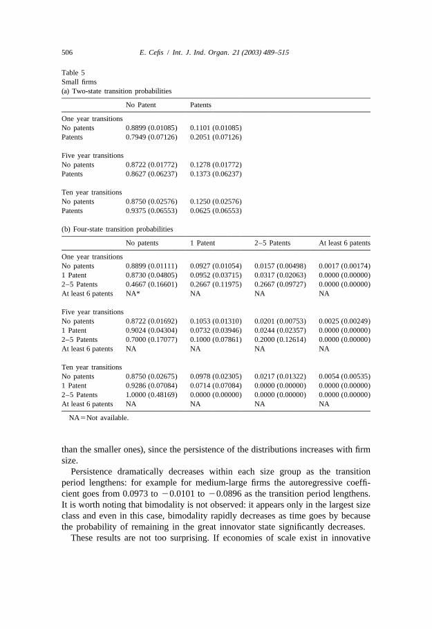
One observes also important differences in persistence across size classes (seeTables 5 and 6): in general, persistence increases as size increases. Theautoregressive coefficient increases as size increases: for a one year transitionperiod, it is 0.0973 for small firms, 0.2212 for medium firms, 0.3143 formedium-large firms, and 0.4866 for large firms. The difference in persistenceacross size classes is maintained as the transition period lengthens. This result is inline with the Schumpeter Mark II hypothesis (the larger firms are more innovative


Table 5Small firms(a) Two-state transition probabilities

No Patent Patents






One year transitionsNo patents 0.8899 (0.01111) 0.0927 (0.01054) 0.0157 (0.00498) 0.0017 (0.00174)1 Patent 0.8730 (0.04805) 0.0952 (0.03715) 0.0317 (0.02063) 0.0000 (0.00000)2–5 Patents 0.4667 (0.16601) 0.2667 (0.11975) 0.2667 (0.09727) 0.0000 (0.00000)At least 6 patents NA* NA NA NA

Five year transitionsNo patents 0.8722 (0.01692) 0.1053 (0.01310) 0.0201 (0.00753) 0.0025 (0.00249)1 Patent 0.9024 (0.04304) 0.0732 (0.03946) 0.0244 (0.02357) 0.0000 (0.00000)2–5 Patents 0.7000 (0.17077) 0.1000 (0.07861) 0.2000 (0.12614) 0.0000 (0.00000)At least 6 patents NA NA NA NA

Ten year transitionsNo patents 0.8750 (0.02675) 0.0978 (0.02305) 0.0217 (0.01322) 0.0054 (0.00535)1 Patent 0.9286 (0.07084) 0.0714 (0.07084) 0.0000 (0.00000) 0.0000 (0.00000)2–5 Patents 1.0000 (0.48169) 0.0000 (0.00000) 0.0000 (0.00000) 0.0000 (0.00000)At least 6 patents NA NA NA NA

NA5Not available.

than the smaller ones), since the persistence of the distributions increases with firmsize.

Persistence dramatically decreases within each size group as the transitionperiod lengthens: for example for medium-large firms the autoregressive coeffi-cient goes from 0.0973 to20.0101 to20.0896 as the transition period lengthens.It is worth noting that bimodality is not observed: it appears only in the largest sizeclass and even in this case, bimodality rapidly decreases as time goes by becausethe probability of remaining in the great innovator state significantly decreases.

These results are not too surprising. If economies of scale exist in innovative


Table 6Large firms(a) Two-state transition probabilities

No Patent Patents









activities, due for instance to the fixed and sunk costs linked to R&D (Cohen andKlepper, 1996), large firms would turn out to be both more innovative and morepersistent. Notice, however, that the direction of causation might well go frompersistence to high innovative performance in the long run rather than the otherway around. The advantage of size might be linked to the fact that e.g. theaccumulation of competencies and infrastructures for R&D generates morepersistent innovative activities over time and hence more innovations, even ifstatic economies of scale are irrelevant or even negative.

For the overall sample, a 20-state TPM was estimated in order to investigatewhether the bimodality was due to right truncation or to the fact that in the last


Table 7Estimates of the first-order autoregressive parameters

r1 r5 r10

Overall 0.32 0.20 0.11Small 0.10 20.01 20.09Medium 0.22 0.05 20.05Medium-large 0.31 0.16 20.06Large 0.49 0.31 0.20Chemical 0.59 0.54 0.53Mechanical engineering 0.20 0.10 20.12Electrical & electronics 0.33 0.20 0.10Instrumental 0.37 0.09 0.02

class there was another mode of the empirical distributions. The bounds of thismatrix were defined as follows: having applied for 0 patents, for 1 patent, for 2–3patents, for 4–5 patents, and so on up to the last state defined as having asked formore than 20 patents. The results show that there still appears evidence ofbimodality due to right truncation.

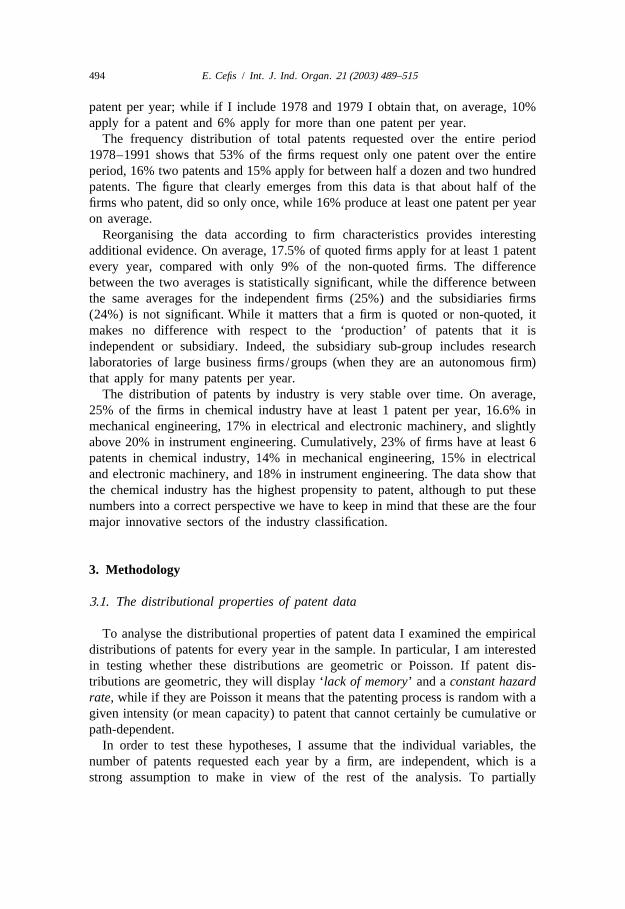
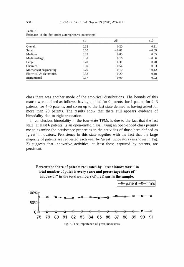
In conclusion, bimodality in the four-state TPMs is due to the fact that the laststate (at least 6 patents) is an open-ended class. Using an open-ended class permitsme to examine the persistence properties in the activities of those here defined as‘great’ innovators. Persistence in this state together with the fact that the largemajority of patents are requested each year by ‘great’ innovators (as shown in Fig.3) suggests that innovative activities, at least those captured by patents, arepersistent.

Fig. 3. The importance of great innovators.


4 .3. The great innovators

Fig. 3 shows pretty clearly the importance of the great innovators in innovativeactivities: they are very few in number (2.37% on average each year), but theyaccount for the large majority of the total number requested each year (77.85% onaverage).

Defining a great innovator as a firm that has applied for 6 or more patent at leastone year over the 14 years of the sample period, I find 40 great innovators over577 firms (7% of the UK random sample).

Considering the industrial classification, the majority of the great innovatorsbelongs to the chemical sector (on average the chemical firms represent the 50% ofthe sample, excluding the first year), followed by the electrical and electronicsector and by the instrumental engineering sector. This rank is not surprising, sinceit reflects exactly the ranking of the sectors in terms of persistence. It is worthnoting that the ranking does not change as time passes and the percentages of firmsbelonging to these sectors remain almost constant over time.

The classification of great innovators according to firm size gives a picture inwhich the large firms play the most important role (on average the percentage oflarge firms is 75%, excluding the first year), followed by the medium-large class.Firms with more than 500 employees represent almost the totality of the greatinnovators. Also in this case the percentages of the size classes are quite stableover time.

For the great innovator sample, two and four state TPMs were estimated for17three transition periods . The estimated probabilities are different from the ones

analysed in the previous section, since these probabilities are conditional on thefact that firms, sooner or later in the sample period, must have applied for at least6 patents. Formally, I have estimated the following probabilities

p 5P(X 5 juX 5 i, maxX > 6) (6)ij t1n t tt

Not surprisingly, two-state TPMs show that there is high persistence, but thatdeclines as the transition period lengthens. Indeed, the first-order autoregressiveparameter goes from 0.66 for a 1-year transition period, to 0.29 for 5 years, to 0.13for 10 years. However, the decline is due to the dramatic decrease of theprobability of remaining in the state in which firms do not apply for a patent.

The same picture is given by the four-state TPMs: there is persistence andbimodality. As the transition period lengthens all the diagonal elements, except the

17TPMs for the great innovator sub-sample may be found in the supplementary material on theIJIO’s Editorial Office web site.


last on the right, decrease quite rapidly, while the probabilities on the right of themain diagonal increase. Moreover, the sum (by row) of the elements out of themain diagonal on the right is always greater than the sum of the elements on theleft. It is more likely that the number of patent applications increases than that itdecreases. It is exactly the opposite of what happens in the TPMs previouslyestimated on the random samples.

5 . Sensitivity analysis

The above analysis has been conducted using various assumptions. In thissection I study whether the results obtained are robust to changes in some of theseassumptions. In particular, I will consider: (i) the possibility that the transitionprobabilities are not time invariant but display structural breaks within the 14 yearsof the sample and (ii) the possibility that the data can be represented by

18second-order Markov chains .Concerning the first assumption, the sensitivity analysis shows time homo-

geneity of the sample and that the features of the TPMs are time invariant,suggesting that (short-term) business cycle considerations have little importancefor qualitative features of the results

As regards the second assumption, the transition probabilities I have consideredthus far allowed the probability measurep to depend on the state at timet 2 1,ij

but not on the state at timet 2 2 or other lagged values. This limitation is not asrestrictive as it may at first seem: any second (or higher) order Markov process(that is, one in which two (or more) lagged values affect the distribution of thecurrent value) can be viewed as a first-order process with an expanded state space(Stokey and Lucas, 1989, Ch. 8.4).

Given this, I consider the possibility that the data can be represented bysecond-order Markov chains. I estimate two and four second-order TPMs,especially in order to see whether they suggest a totally different picture and/orwhether some additional features can emerge from this representation.

Assuming that Markov chains are homogeneous on the parameter space and ofsecond-order, the one-step transition probability is defined by:

p 5P(X 5 juX 5 i, X 5 k) (7)kij t t21 t22

with t51978, 1979,. . . , 1991.The second-order TPMQ is the matrix with p as elements measuring thekij

probability of moving to statej at time t, given that the firm was in statei at timet 2 1, and in statek at time t 22.

18Complete results of the sensitivity analysis may be found in the supplementary material on theIJIO’s web site.


Table 8Overall sample second-order Markov chain(a) Two-state transition probabilities

No patents:X Patents:Xt50 t51

X 5 0, X 5 0 0.8772 0.1228t21 t22

X 5 0, X 5 1 0.7473 0.2527t21 t22

Xt 5 1, X 5 0 0.8365 0.163521 t22

Xt 2151, X 51 0.2919 0.7081t22

(b) four-state transition probabilities

No patents:X 1 Patent:X 2–5 Patents:X >6 Patents:Xt50 t51 t52 t53

X 5 0, X 5 0 0.8905 0.052 0.0141 0.0002t21 t22

X 5 0, X 5 1 0.8170 0.1312 0.0518 0.0000t21 t22

X 5 0, X 5 2 0.6202 0.2558 0.1085 0.0155t21 t22

X 5 0, X 5 3 0.0000 0.0000 0.8571 0.1429t21 t22

X 5 1, X 5 0 0.8182 0.1299 0.0487 0.0032t21 t22

X 5 1, X 5 1 0.6122 0.2245 0.1429 0.0204t21 t22

X 5 1, X 5 2 0.2069 0.3276 0.4483 0.0172t21 t22

X 5 1, X 5 3 0.0909 0.6364 0.0909 0.1818t21 t22

X 5 2, X 5 0 0.1414 0.7238 0.1309 0.0039t21 t22

X 5 2, X 5 1 0.7856 0.1455 0.0657 0.0031t21 t22

X 5 2, X 5 2 0.4920 0.2781 0.2139 0.0160t21 t22

X 5 2, X 5 3 0.0909 0.0909 0.5454 0.2727t21 t22

X 5 3, X 5 0 0.5385 0.1538 0.2301 0.0769t21 t22

X 5 3, X 5 1 0.0769 0.2308 0.3846 0.3077t21 t22

X 5 3, X 5 2 0.0833 0.0278 0.3611 0.5278t21 t22

X 5 3, X 5 3 0.0000 0.0165 0.0661 0.9174t21 t22

The second-order TPMs display overall features which are similar to first-orderones. As Table 8 shows, in the two-state TPM, the probabilities of being in thepolar states, that is the probability of having applied for no patents given that inthe two previous years the firm has not applied for a patent as well as theprobability of having applied for at least one patent given that in the previous twoyears the firm has applied for at least one patent, are very large, suggestingstronger persistence and bimodality features than those displayed by first-orderTPMs. There is stronger evidence of heterogeneity across the dimension of thesample and especially across industrial classification (see Table 8).

The four-state TPMs reinforce the results obtained by two-state TPMs: there ismore persistence and more bimodality. For example, in the chemical industry theprobability of applying for no patent given that the firm has not applied for apatent in the previous two years is 0.9042, and the probability of applying for atleast six patents given that the firm has applied for at least six patents in theprevious two years is 0.9740, while in the mechanical industry the two prob-abilities are respectively 0.8825 and 0.50. There is another interesting feature thatsuggests a stronger persistence in innovative activities: the probability of applying


for no patent given the fact that in the previous two years the firm has applied forat least six patents is always 0, and, vice versa, the opposite probability ofapplying for at least six patents given that in the previous two years the firm hasnot applied for a patent is always 0 or almost 0, for the overall sample and forevery sub-sample across size and industrial classification.

This result suggests that firm innovative activities are cumulative and path-dependent: it is quite difficult for a ‘great’ innovator to lose suddenly all itsinnovative capabilities and to exhaust all its innovating opportunities, and viceversa it is quite difficult for a firm that has innovated once in a while in the past tobecome suddenly a firm that has knowledge and organisational capabilities toinnovate on a continuous basis.

The estimation of second-order Markov chains suggests that the patenting19process is not a first-order Markov process . Indeed, if it were the case, the

conditional probabilities of moving from timet 21 to time t among states wouldnot have depended on the state in which the firm was at timet 22 and theestimated probabilities would have been very similar. The actual estimatedprobabilities, instead, show that the probabilities of moving from one state toanother depend crucially on the state in which the firm was in previous periods.This observation suggests that a longer history matters in determining firms’current innovative activities than simply the state in the last period.

6 . Conclusions

The paper analysed the statistical properties of the stochastic process generatingthe patent time series of UK manufacturing firms. Although the empiricaldistributions of patents for every year in the sample look geometric, the geometricdistribution is rejected. The distributions do not display the lack-of-memoryproperty and show decreasing hazard rate and, therefore, negative durationdependence.

This result suggests that there exists a threshold to patenting and the threshold isrepresented by the first patent. The probability of going from zero to one patentapplication is uniformly much lower than the probability of going fromn to n 1 1patents, withn >1. Moreover, applying for an additional patent becomes easier (inthe sense that the probability to get an additional patent becomes higher) as thenumber of patent applications becomes higher. This can be interpreted assuggesting that once the threshold is crossed, innovative activities carried outinside the firm enjoy economies of scale.

For the overall sample, TPMs show that there is little persistence (but notnegligible) in general, but a strong bimodality. That is, there is a high probability

19However, this does not mean that the estimated first-order TPMs lose their ‘descriptive’ validity:we are just saying that the process that generates the patent series is not a first-order Markov process.


of remaining in the polar states, namely in the states in which firms do not applyfor a patent (the ‘occasional innovator’ state) and in which firms apply for at leastsix patents (the ‘great innovator’ state), especially the longer is the transitionperiod. This result, together with the observation that the large majority of patentsare requested each year by ‘great innovators’, suggests that innovative activities, atleast those captured by patents, are persistent.

There is evidence of heterogeneity across the industrial classification and sizedimensions of the sample. Differences in the estimated entries of the TPMs areparticularly important across industrial sectors. The patent data show that in thechemical sector there is a high probability of remaining in the state in which thefirms started regardless of the length of the transition period and the bimodality ofthe estimated TPMs is striking. In the mechanical engineering sector the state inwhich firms have not applied for patents is almost an absorbing state. Thissuggests that innovative activities are sector specific, that is, they proceeddifferently across industries: in some sectors persistence is very low, in othersquite high. In line with the Schumpeter Mark II hypothesis, persistence tends toincrease monotonically with firm size, with large firms being more persistent thansmall firms.

Finally, the estimated second-order Markov chains suggest that firm innovativeactivities are path-dependent: it is quite difficult for a ‘great’ innovator to losesuddenly all its innovative capabilities and to exhaust all its innovating oppor-tunities, and vice versa it is quite difficult for a firm that has innovated once in awhile in the past to become suddenly a firm that has knowledge and organisationalcapabilities to innovate on a continuous basis.

The analysis previously presented should be considered as a piece of evidencetowards a systematic analysis of the sources and implications of persistence ininnovative activities. Indeed, so far, we know nothing about the determinants ofpersistence and these results do not allow us to draw any strong theoreticalconclusions. Yet, on the whole, these findings suggest that innovation is not apurely random phenomenon driven by small shocks, but it implies systematicheterogeneity across firms and/or some forms of dynamic increasing returns.

Among firms that innovate (the majority do not innovate), many do so onlyoccasionally and very few persistently. Innovating is difficult and persistentinnovating is even more difficult. Even for great innovators it is often hard tomaintain their innovativeness over prolonged periods of time. However, persistentinnovators (large and small) originate a high share of all innovative activities.

From a theoretical point of view, we might interpret these results as supportingthe theory of ‘dynamic capabilities’, in which innovative performance is generatedand has to be supported by systematic and continuous processes of accumulationof resources and competencies over time (Teece and Pisano, 1994), more than the‘competence-based’ theory of the firm (Nelson and Winter, 1982).

From a normative perspective, these results show that great innovators arepersistent innovators. This might imply either that persistence is an important


ingredient for high innovative performance or that success in innovation breedsfurther success. In both cases, these results suggest the hypothesis that persistencerather than the size of firms or the size of investments in innovative activities perse might be an appropriate target for economic policies supporting innovation andfor managerial strategies.

A cknowledgements

I am particularly grateful to Soren Johansen, Franco Malerba, Luigi Orsenigoand Luis Phlips for encouragement and helpful suggestions. I would also like tothank Giovanni Dosi, Giuseppe Espa, Luigi Marengo, Stephen Martin, ChiaraMonfardini, Danny Quah for interesting comments. This is a substantially revisedversion of a paper presented at RES 96, IGIER 96, EEA 96, ESEM 96, EARIE 96,University of Trento 98, and at Universitat Pompeu Fabra 98. I thank theparticipants and the seminar audiences for useful comments. The financial supportof the EU TRM program, ERBFMBICT 96-0805, and of the University ofBergamo (grant ex 60%, n. 60CEFI01), Dept. of Economics) is gratefullyacknowledged.

R eferences

Amemiya, T., 1994. Introduction to Statistics and Econometrics. Harvard University Press, Cambridge,MA.

Baily, M.N., Chakrabarty, A.K., 1985. Innovation and productivity in US industry. Brookings paperson Economic Activity 2, 609–632.

Barro, R., Sala-i-Martin, X., 1995. Economic Growth. McGraw Hill, New York.Bottazzi, G., Dosi, G., Lippi, M., Pammolli, F., Riccaboni, M., 2001. Innovaton and corporate growth

in the evolution of the drug industry. International Journal of Industrial Organization 19 (7),1161–1187.

Bottazzi, G., Cefis, E., Dosi, G., 2002. Corporate growth and industrial structures: some evidence fromthe Italian manufacturing industry. Industrial and Corporate Change 11 (4), 705–723.

Cefis, E., 1999. Persistence in innovative activities. An empirical analysis. Ph.D. Thesis, EuropeanUniversity Institute, Florence.

Cefis, E., 2001. Persistence in innovation and profitability. Submitted to Rivista Internazionale diScienze Sociali.

Cohen, W.M., Klepper, S., 1996. A reprise of size and R&D. Economic Journal 106 (437), 925–951.Coriat, B., Dosi, G., 1998. Learning how to govern and learning how to solve problems: on the

co-evolution of competences, conflicts and organizational routines. In: Chandler, A.D., Hagstrom, P.,Solvell, O. (Eds.), The Dynamic Firm: The Role of Technology, Strategy, Organization, andRegions. Oxford University Press, Oxford.

Dosi, G., 1988. Sources, procedures and microeconomic effects of innovation. The Journal ofEconomic Literature 26 (3), 1120–1171.

Cubbin, J., Geroski, P., 1987. The convergence of profits in the long run: inter-firm and inter-industrycomparisons. Journal of Industrial Economics 35 (4), 427–442.


Dosi, G., Marsili, O., Orsenigo, L., Salvatore, R., 1995. Learning, market selection and the evolution ofmarket structure. Small Business Economics 7, 411–436.

Ericson, R., Pakes, A., 1992. An alternative theory of the firm and industry dynamics. CowlesFoundation Discussion Paper No. 1041, Cowles Foundation for Research in Economics at YaleUniversity.

Geroski, P., Jacquemin, A., 1988. The persistence of profits: a European comparison. Economic Journal98, 375–389.

Geroski, P., Machin, S., Van Reenen, J., 1993. The profitability of innovating firms. RAND Journal ofEconomics 24 (2), 198–211.

Geroski, P.A.,Van Reenen, J., Walters, C.F., 1997. How persistently do firms innovate? Research Policy26 (1), 33–48.

Griliches, Z., 1986. Productivity, R&D and basic research at the firm level in 1970s. AmericanEconomic Review 76, 141–154.

Hopenhayn, H.A., 1992. Entry, exit and firm dynamics in long run equilibrium. Econometrica 60 (5),1127–1151.

Jovanovic, B., 1982. Selection and the evolution of industry. Econometrica 50 (3), 649–670.Klepper, S., 1996. Entry, exit and innovation over the product life cycle. American Economic Review

86 (3), 562–582.Malerba, F., Orsenigo, L., 1999. Technological entry, exit and survival. Research Policy 28, 643–660.Martin, S., 2001. Advanced Industrial Economics, 2nd Edition. Blackwell, Oxford and Cambridge,

MA.Mueller, D.C., 1990. Profits and the process of competition. In: Mueller, D. (Ed.), The Dynamics of

Company Profits: An International Comparison. Cambridge University Press, Cambridge.Nelson, R., Winter, S., 1982. An Evolutionary Theory of Economic Change. The Bellknap Press of

Harvard University Press, Cambridge, MA.Odagiri, H., Yamawaki, H., 1990. The persistence of profits in Japan. In: Mueller, D.C. (Ed.).Patel, P., Pavitt, K., 1991. Europe’s technological performance. In: Freeman, et al. (Ed.), Technology

and the Future Of Europe: Global Competition And The Environment in the 1990s. Pinter Publisher,London.

Quah, D., 1993a. Empirical cross-section dynamics in economic growth. European Economic Review37, 426–434.

Quah, D., 1993b. Galton’s fallacy and tests of the convergence hypothesis. Scandinavian Journal ofEconomics 4, 427–443.

Schumpeter, J.A., 1934. The Theory of Economic Development. Harvard Economic Studies, Cam-bridge MA.

Schumpeter, J.A., 1942. Capitalism, Socialism and Democracy. Harper and Brothers, New York.Silverman, B.W., 1986. Density Estimation for Statistics and Data Analysis. Chapman and Hall,

London.Stokey, N.L., Lucas, R.E., 1989. Recursive Methods in Economic Dynamics. Harvard University Press,

Cambridge, MA.Teece, D., Pisano, G., 1994. The dynamic capabilities of firms: an introduction. Industrial and

Corporate Change 3 (3), 537–555.Wilk, M.B., Gnanadesikan, R., 1968. Probability plotting methods for the analysis of data. Biometrika

55, 1–17.Winter, S., 1984. Schumpeterian competition in alternative technological regimes. Journal of Economic

Behaviour and Organization 5 (3–4), 287–320.

Is there persistence in innovative activities

Documents

Transcript of Is there persistence in innovative activities