arX

iv:0

805.

2698

v1 [

nlin

.PS]

17

May

200

8

Solitons and vortices in honeycomb defocusing photonic lattices

K. J. H. Law,1 H. Susanto,2 and P. G. Kevrekidis1

1Department of Mathematics and Statistics, University of Massachusetts, Amherst MA 01003-4515, USA2 School of Mathematical Sciences, University of Nottingham, University Park, Nottingham, NG7 2RD, UK

Solitons and necklaces in the first band-gap of a two-dimensional optically induced honeycombdefocusing photonic lattice are theoretically considered. It is shown that dipoles, soliton necklaces,and vortex necklaces exist and may possess regions of stable propagation through a photorefractivecrystal. Most of the configurations disappear in bifurcations close to the upper edge of the firstband. Solutions associated with such bifurcations are also numerically examined, and it is foundthat they are often asymmetric and more exotic. The dynamics of the relevant unstable structuresare also examined through direct numerical simulations revealing either breathing oscillations or, insome cases, destruction of the original waveform.

PACS numbers:

I. INTRODUCTION

In the past few years, there has been a considerablegrowth of interest in the examination of the self-trappingof light in photonic lattices optically induced in nonlin-ear photorefractive crystals, such as strontium bariumniobate (SBN). This can be attributed to a considerableextent to the fact that the theoretical inception [1] ofthe relevant phenomena was rapidly followed by the ex-perimental realization [2, 3, 4], revealing a considerablewealth of new possibilities. This setting naturally per-mits the consideration of the competition between ef-fects of nonlinearity and those of diffraction, thereforeenabling the examination of effects of periodic “poten-tials” on solitary waves. In this context the role of theeffective potential is played by the ordinary polarizationof light forming a waveguide array in which the nonlinear,extra-ordinarily polarized probe beam evolves.

Numerous nonlinear waves and coherent structureshave been elucidated and experimentally realized in thiscontext. In particular, discrete dipole [5], necklace [6]solitons and even stripe patterns [7], rotary solitons [8],discrete vortices [9] or the realization of photonic qua-sicrystals [10] and Anderson localization [11] are amongthe recently reported experimental results in the field.These efforts illustrate the potential that this settingholds for the examination of localized structures that maybe usable as carriers and conduits for data transmissionand processing in all-optical communication schemes. Inparallel to this more practical aspect, this frameworkremains an experimentally tunable playground wherenumerous fundamental issues of solitons and nonlinearwaves can be explored.

The above mentioned interplay of nonlinearity with pe-riodicity is important not only in the physics of opticallyinduced lattices in photorefractive crystals, but also in avariety of other contexts in optical and atomic physics.These involve e.g. on the optical end, the numerous de-velopments on the experimental and theoretical investi-gation of optical waveguide arrays; see e.g. [12, 13] forrelevant reviews. In the case of atomic physics, and par-ticularly of Bose-Einstein condensates, the confinement

of dilute alkali vapors in optical lattice potentials [14]has offered a similarly far-reaching opportunity to exam-ine many fundamental phenomena involving (effective)nonlinearity and spatial periodicity. These include, butare not limited to modulational instabilities, Bloch oscil-lations, Landau-Zener tunneling and gap solitons amongothers; see [15] for a recent review.

Our present study, motivated by optically induced lat-tices in photorefractive SBN crystals, focuses on two-dimensional periodic, nonlinear media with a non-square

lattice. While most of the above studies have been ded-icated to square lattices, only a few have tackled thecoherent structures possible in non-square settings; seee.g., as relevant examples [16, 17, 18, 19, 20, 21] and ref-erences therein. Furthermore, the vast majority of theabove-mentioned studies has centered around focusingnonlinearities. At least partly, this is due to technicallimitations, as it is easier to work with voltages that arein the regime of focusing rather than in that of the defo-cusing nonlinearity (in the latter case, sufficiently largevoltage, which is tantamount to large nonlinearity, mayactually change the sign of the nonlinearity by invertingthe orientation of the permanent polarization of the crys-tal). As a result, coherent structures in the defocusingregime, have only rather sparsely been examined. Suchan experimental example is the fundamental and higherorder gap solitons excited in the vicinity of the edge ofthe first Brillouin zone [2, 21]. More complex gap struc-tures (multipoles and vortices) are only now starting tobe explored in square lattices [22]. In parallel to theseexperimental developments, a theoretical framework isstarting to emerge to address such multipole and vor-tex structures in square lattices with cubic nonlinearities[23, 24], whose qualitative predictions can however be ex-tended to non-square settings and the main ones amongwhich will also be compared to the results presented be-low. Our main focus in the present work is on employinga continuum model to examine the waveforms present ina context involving a triangular lattice (honeycomb ) po-tential and a saturable defocusing nonlinearity associatedwith appropriate optically induced lattices in SBN crys-tals. In particular, we study in detail multipole (dipole

2

and hexapole) solitons in such lattices induced with aself-defocusing nonlinearity.

We numerically analyze both the existence and the sta-bility of these structures and follow their dynamics, in thecases where we find them to be unstable. We also quali-tatively compare our findings with the roadmap providedby the discrete model [23].

Our presentation is structured as follows. In sectionII, we present our theoretical model setup. Dipole solu-tions with the two excited sites in adjacent wells of theperiodic potential (nearest-neighbor dipoles) are studiedin section III. Subsequently, we do the same for next-nearest-neighbor dipoles (excited in two diagonal sites,separated by one lattice site) in section IV and oppositedipoles on either end of the hexagonal configuration (ie.the excited sites are separated by two empty wells) insection V. Section VI addresses the case of more com-plex structures such as hexapoles (all six sites from oneperiod of the potential) and vortices. Finally, in sectionVII, we summarize our findings, posing some interestingquestions for future study.

II. SETUP

We use the standard partial differential equation forthe amplitude of the electric field U [19, 20, 25, 26], inthe following form:

− iUz = [L + N(x, |U |2)]U, (1)

N(x, |U |2) =E0

1 + I(x) + |U |2 , (2)

where L = D∇2 and ∇2 is the two-dimensional Lapla-cian, U is the slowly varying amplitude of the probebeam, and

I(x) = I0

∣

∣eikb1x + eikb2x + eikb3x∣

∣

2

(3)

is the optical lattice intensity function formed by three

laser beams with b1 = (1, 0), b2 = (− 1

2,−

√3

2), and

b3 = (− 1

2,√

3

2). Here I0 is the lattice peak inten-

sity, z is the propagation distance and x = (x, y) aretransverse distances (normalized to zs = 1 mm andxs = ys = 1µm), E0 is proportional to the applied DCfield voltage, D = zsλ/(4πnexsys) is the diffraction co-efficient, λ is the wavelength of the laser in a vacuum, dis the period in the x direction with k = 4π/(3d) (period

in the y direction is√

3d), and ne is the refractive indexalong the extraordinary axis. We choose the lattice in-tensity I0 = 0.6. A plot of the optical lattice is shownin Fig. 1 for illustrative purposes regarding the locationwhere our localized pulses will be “inserted”. In addition,we choose other physical parameters consistently with atypical experimentally accessible setting [19, 22] as

d = 30µm, λ = 532 nm, ne = 2.35, E0 = 8.

The non-dimensional value D = 18.01, and we notethat this dispersion coefficient is equivalent to rescalingspace by a factor

√D as e.g. in [27].

The numerical simulations are performed in a rectan-gular domain corresponding to the periodicity of the lat-tice using a rectangular spatial mesh with ∆x ≈ 0.75 and∆y ≈ 0.86 and domain size 4d×3

√3d, i.e. 160×180 grid

points. See Fig. 1 for a schematic of the spatial configu-rations.

Regarding the typical dynamics of a soliton when it isunstable, we simulate the z-dependent evolution using aRunge-Kutta fourth-order scheme with a step ∆z = 0.01.

x

y

−40 −20 0 20 40

−50

0

50 0

1

2

3

4

5

A

E

B

DC

F

FIG. 1: (Color online) A spatial (x-y) contour plot of the or-dinary polarization standing wave [lattice beam in Eq. (3)].In this context, the light intensity maxima correspond to theminima of the resulting refractive index lattice (i.e., honey-comb lattice), as opposed to the focusing nonlinearity latticefield, where they correspond to the maxima (i.e., triangularlattice). Points A, B, C, D, E, and F are used for namingthe various configurations. A is a “nearest-neighbor” mini-mum of B and F , a “next-nearest-neighbor” of C and E, andan “opposite” of D (with respect to the local maximum ofthe lattice). Because of the symmetry of the setup, this isa complete characterization of dipole configurations. We willrefer to the configurations with the names given above.

Assuming a stationary state u(x, y) exists, and lettingthe propagation constant µ represent the (nonlinear) realeigenvalue of the operator of the right-hand-side of Eq.(1), then the corresponding eigenvector u(x, y) is a fixedpoint of

[µ − L − N(x, |u|2)]u = 0. (4)

The localized states u of (4) were obtained using theNewton-GMRES fixed point solver nsoli from [28] and

3

a pseudo arc-length continuation [29] was used to followeach branch and locate the bifurcations which occur atthe edge of the first band. Since the parameter of interestis µ, diagnostics are plotted against µ.

We restrict µ to those values within the first spectralgap of the linear eigenvalue problem,

[µ − L − N(x, 0)]u = 0. (5)

Values of the propagation constant µ within this for-bidden gap in the spectrum of the linearized problem willcorrespond to exponentially localized in space, so-calledgap-soliton, states of the original nonlinear partial dif-ferential equation. Using a standard eigenvalue solverpackage implemented through MATLAB, we identify thespectral gap for our given parameters and gridsize to be3.62 . µ . 4.94.

The square root of the optical power (or, mathemat-ically, the L2 norm) of the localized waves is defined asfollows:

P =

[∫ ∞

−∞

∫ ∞

−∞

|U |2 dx dy

]1/2

. (6)

Introducing a linearization around an exact stationarysolution u, and expanding the leading order perturba-tion into a eigenfunctions and eigenvalues, we obtain thefollowing Bogoliubov system

[

iλ + µ − L − ∂(NU)

∂U|u

]

u − ∂(NU)

∂U∗|uu∗ = 0,

[

iλ − µ + L +∂(NU)∗

∂U∗|u

]

u∗ +∂(NU)∗

∂U|uu = 0.(7)

We solve the above linear eigenvalue problem using MAT-LAB’s standard eigenvalue solver package. The symplec-tic nature of the resulting eigenvalue equations guaran-tees that the relevant eigenvalues should come in quar-tets, hence an instability is present whenever the solutionof the above linearization problem of Eqs. (7) possessesan eigenvalue with a non-zero real part.

We now briefly discuss the principal stability conclu-sions, for the defocusing case of [23], which we should ex-pect to still be valid in the present configuration. Nearestneighbor excitations in the defocusing case correspondto nearest neighbor excitations in the focusing case, butwith an additional π phase in the relative phase of thesites added by the so-called staggering transformation[23]. Therefore, the in-phase nearest neighbor config-uration in the defocusing case corresponds to an out-of-phase such configuration in the focusing case (andshould thus be stable) [24]. On the other hand, nextnearest neighbor out-of-phase defocusing configurationswould correspond to next nearest neighbor out-of-phasefocusing configurations and should also be stable (at leastin some parameter regimes). By the same token, out-of-phase nearest neighbor, and in-phase next nearest neigh-bor structures should be unstable. These considerations

also indicate that in-phase opposite dipoles should bestable, while out-of-phase such dipoles should always beunstable. Finally, vortex-like structures and in-phasehexapoles should be stable as well. Notice, however, thatas discussed in [23] the multipole structures characterizedas potentially stable above will, in fact, typically possessimaginary eigenvalues of negative Krein signature (seee.g. [30] and references therein). These may lead to os-cillatory instabilities through complex quartets of eigen-values. These arise by means of Hamiltonian-Hopf bifur-cations [31] emerging from collisions with eigenvalues ofopposite (i.e., positive) Krein signature. These conclu-sions will be discussed in connections with our detailednumerical results in what follows.

III. NEAREST NEIGHBOR DIPOLE SOLITONS

In this section, we report dipole solitons where the twolobes of the wave are located in two nearest neighbor(N) lattice sites in the 2D triangular potential shown inFig. 1. The lobes can have the same phase or π phasedifference so we define them as in-phase (IP) dipoles andout-of-phase (OP) dipoles, respectively.

A. In-Phase Nearest Neighbor Dipole Solitons

We have found IP dipoles in adjacent wells for values ofthe propagation constant µ throughout the entire Braggreflection gap for a given E0. We found that the solitonsexist for µ between 3.62 and 4.94, and that the intensityof the dipoles cannot be arbitrary low, a result similar tothe observed results of the focusing and defocusing casesfor square lattices [5, 26, 27]. The relevant findings aresummarized in Fig. 2.

The top left panel of Fig. 2 shows the stability of thedipoles against the propagation constant µ, by illustrat-ing the maximal growth rate (maximum real part of alleigenvalues λ) of perturbations. When max(Re(λ)) = 0,this implies stability of the configuration, while the con-figuration is unstable if max(Re(λ)) 6= 0 in this Hamilto-nian system. We found that this type of dipoles may bestable for windows throughout the first Bragg gap, as pre-dicted above, although it is possible for small oscillatoryHopf instabilities to arise due to opposite signature eigen-value collisions. The dipole configuration disappears in asaddle-node bifurcation at the edge of the first spectralband, depicted in the top panels of Fig. 2, as µ → 4.94,and a real pair of eigenvalues emerges. At this point,the configuration collides with a configuration shown atthe bottom panel of Fig. 2 in which the adjacent wellnext to one of the populated ones becomes excited out-of-phase with the others. Consistent with our theoreticalexpectation from its having an out-of-phase set of near-est neighbors, the latter configuration always has a realpair of eigenvalues λ.

4

3.5 4 4.5 50

0.1

0.2

0.3

0.4m

ax(R

e(λ)

)

µ3.5 4 4.5 5

0

5

10

15

P

µ

x

y

−50 0 50

−60

−40

−20

0

20

40

60

0

0.2

0.4

0.6

−1 −0.5 0 0.5 1

x 10−3

−1

−0.5

0

0.5

1

λr

λ i

x

y

−50 0 50

−60

−40

−20

0

20

40

60

−0.6

−0.4

−0.2

0

0.2

0.4

0.6

−0.2 0 0.2

−1

−0.5

0

0.5

1

λr

λ i

FIG. 2: (Color online) The top left panel shows the stabil-ity of the dipoles against the propagation constant µ. Itis stable when the spectra is purely imaginary (i.e., whenmax(Re(λ)) = 0). The top right panel depicts the powerof the dipoles against the propagation constant. In each ofthese images the solution branch is denoted by a solid line.The branch with which the dipole collides and terminates ina saddle-node bifurcation is shown by a dashed line. Theshaded areas in both of these panels represent the bands oflinear spectrum (5). The middle left and right panels showthe profile u of the dipole at µ = 4 and the correspondingcomplex spectral plane (Re(λ), Im(λ)) of λ = Re(λ)+ iIm(λ).Finally, the bottom panels show the same features for theunstable saddle solution corresponding to the dashed line.

The middle left and right panels show the profile uof the in-phase nearest (IPN) neighbor dipole at µ = 4and the corresponding spectrum of linearization eigen-values λ = λr + iλi in the complex plane (λr , λi), re-spectively. The corresponding profile and spectral planefor the saddle branch (that eventually collides with theIPN solution) at µ = 4 is shown in the bottom left andright panel, respectively, of the same figure, illustratingthe exponential instability of the latter.

We have simulated the dynamics of the solitary waveswhen they are unstable. The dipoles are perturbed bya random noise with maximum intensity 2 × 10−3. Itis interesting to note that an unstable IPN dipole turnsout to be quite robust, even though it experiences onlyan oscillatory instability. It is remarkable that up toz = 200 we did not see any signifant change in the con-figuration. Therefore, we do not depict our evolutionsimulation here; we simply note that this is consonantwith the very weak growth rate of the relevant oscilla-

FIG. 3: The typical time-dependent dynamics of an unstableconfiguration along the upper (dashed line) branch of the ex-istence curve presented in the top panels of Fig 2. Depictedhere is the isosurface of height 0.15 of the dynamics of the ofthe intensity, |U |2, of the configuration shown in the bottompanel of Fig. 2.

3.5 4 4.5 50

0.1

0.2

0.3

0.4

0.5

0.6m

ax(R

e(λ)

)

µ3.5 4 4.5 5

0

2

4

6

8

10

P

µ

x

y

−50 0 50

−60

−40

−20

0

20

40

60

−0.6

−0.4

−0.2

0

0.2

0.4

0.6

−0.2 0 0.2

−1

−0.5

0

0.5

1

λr

λ i

FIG. 4: (Color online) The top panels correspond to the samepanels of Fig. 2 but for OPN dipole solitons. The bottompanels show the profile u and the corresponding spectral planeof the dipoles at µ = 4.

tory instability.

For the solution branch shown in the bottom panel ofFig. 2, we present its dynamics in Fig. 3. We found thatthe instability is strong as predicted above such that evenafter a relatively short propagation distance, the insta-bility already sets in and leads to recurrent oscillations(for the remainder of our dynamical evolution horizon)between a dipole, two-site state and a three-excited-sitestate; see Fig. 3.

5

FIG. 5: The typical dynamical evolution of an unstable out-of-phase nearest neighbor configuration from the family pre-sented in Fig 4. Depicted is the isosurface at half the maxi-mum of the intial intensity amplitude. Notice that the OPNappears to oscillate between two sites and one for the prop-agation constant µ = 4 (center) of the solution presentedin the bottom panels of Fig. 4, as does it for smaller values(µ = 3.6, left), although for a larger value of µ = 4.6, right,the solution essentially transforms (due to the instability) intoa single site mode. We hypothesize that the stronger effectof the nonlinearity on those solutions with smaller values ofµ decreases the size of linear regime, causing these more lin-early unstable solutions to actually appear more stable in thefull nonlinear dynamical evolution, although it is away fromthe linear regime that the instability is manifested merely asoscillations.

B. Out of Phase Nearest Neighbor Dipole Solitons

We have also found OP dipoles arranged in nearest-neighboring lattice wells which we refer to as OPN. Wesummarize our findings in Fig. 4 where one can see thatthe solitons exist in the whole entire region of propaga-tion constant µ in the first Bragg gap, µ ∈ (3.62, 4.94).This smooth transition indicates that the OPN dipolesolitons emerge out of the Bloch band waves; see e.g. [32]and [33] for a relevant discussion of the 1D and of the 2Dproblem respectively, in the case of the cubic nonlinearity.The OPN dipoles are unstable due to a real eigenvaluepair, as expected from our above theoretical predictions.

As the branch merges with the band edge, we observean interesting feature, namely that the configuration be-gins to resemble a hexapole with a π phase differencebetween each well. This can be an indication that thesestructures bifurcate out of the Bloch band from the samebifurcation point. We elaborate this further in our dis-cussion at the end of section VI.

In Fig. 5 we present the unstable dynamics of OPNdipole solitons perturbed by similar random noise per-turbation as in Fig. 3. We display here three solutionsfor a range of chemical potentials to illustrate that thedynamical evolution of linearly unstable states is appar-ently correlated to the power of the solution. This type

of dipoles is typically more unstable than its IP counter-part, as is illustrated in the figure. In particular, in allthree examples of unstable evolution given the instabilityalready starts to manifest itself. around z = 20 However,for small values of µ (large power) the OPN continuesoscillating between a single site structure and a two sitestructure for the (longer) evolution distances investigatedin this illustrative case, while for large enough µ (smallenough power), one of the sites decays and the power isconcentrated on a single site.

IV. NEXT NEAREST NEIGHBOR DIPOLE

SOLITONS

We have also obtained dipole solutions that are notoriented along the two nearest-neighboring lattice wells,but rather where the two humps of the structure are lo-cated at two next-nearest-neighboring lattice sites. Thesehumps can once again have the same phase or a π phasedifference between them. We will again use the corre-sponding IP and OP designations for these next nearestneighbor waveforms.

A. In Phase, Next Nearest Neighbor Dipole

Solitons

The in-phase next-nearest (IPNN) neighbor solitonsexist only up to a marginal distance from the secondband. The stability and power of these dipoles are shownin Fig. 6. The stability is again consistent with the the-oretical discussion of Section II. In particular, the IPNNconfiguration always possesses a real eigenvalue pair; fur-thermore, the corresponding unstable “saddle” structurewith which it collides and terminates through a saddle-node bifurcation has an additional such eigenvalue pair(two real eigenvalue pairs in total for the solution branchindicated by dashed line in Fig. 6).

We have simulated also the dynamics of the unstableIPNN. Yet, we do not present our simulation here as thetypical evolution of this configuration is quite in resem-blance to the dynamics of an unstable OPN (see Fig. 5) inthe fact that the configuration recurrently oscillates be-tween a two-soliton state and a one-soliton state. Suchan oscillation persists even up to z = 200.

In Fig. 7, we present the dynamical evolution of the bi-furcating solution shown in the bottom panel of Fig. 6 un-der similar random noise perturbation as above. One cannote similarities in the typical evolution of this configu-ration and the evolution of the bifurcating IPN solutionshown in Fig. 3, one of which is the recurrent oscillationbetween a pattern with three pulses and one with justtwo peaks.

6

3.5 4 4.5 50

0.1

0.2

0.3

0.4m

ax(R

e(λ)

)

µ3.5 4 4.5 5

0

2

4

6

8

10

12

P

µ

x

y

−50 0 50

−60

−40

−20

0

20

40

60

0

0.2

0.4

0.6

−0.1 0 0.1

−1

−0.5

0

0.5

1

λr

λ i

x

y

−50 0 50

−60

−40

−20

0

20

40

60

−0.4

−0.2

0

0.2

0.4

0.6

−0.4 −0.2 0 0.2 0.4

−1

−0.5

0

0.5

1

λr

λ i

FIG. 6: (Color online) The top panels correspond to the samediagnostics as in Fig. 2 but for IPNN dipole solitons. The mid-dle panels show the profile U and the corresponding spectralplane of the IPNN dipole at µ = 4.1, while the bottom rowshows the same images for the solution branch correspondingto the dashed line in the top panel, shown at the same valueof µ.

FIG. 7: The same figure as Fig. 3, but for the solution pre-sented in the bottom panel of Fig. 6. Depicted is the isosurfaceof height 0.05.

B. Out of Phase Next Nearest Neighbor Dipole

Solitons

We have also obtained out-of-phase, next-nearest(OPNN) neighbor dipole solitons. A typical profile of

3.5 4 4.5 50

0.1

0.2

0.3

0.4

max

(Re(

λ))

µ3.5 4 4.5 5

0

5

10

15

P

µ

x

y

−50 0 50

−60

−40

−20

0

20

40

60

−0.6

−0.4

−0.2

0

0.2

0.4

0.6

−1 −0.5 0 0.5 1

x 10−3

−0.5

0

0.5

λr

λ i

x

y

−50 0 50

−60

−40

−20

0

20

40

60

−0.6

−0.4

−0.2

0

0.2

0.4

0.6

−0.4 −0.2 0 0.2 0.4

−0.5

0

0.5

λr

λ i

FIG. 8: (Color online) The top panels depict the largest realpart of the critical eigenvalue, as well as the power of theOPNN dipole solitons. The middle panels show the profileu and the corresponding spectra in the complex plane of thedipole at µ = 3.9, and the bottom is the unstable saddleconfiguration at the same value of µ, where one of the siteshas merged with a neighbor out of phase and become an OPN,accounting for the real eigenvalues.

FIG. 9: The same figure as Fig. 3, but for the solution pre-sented in the bottom panel of Fig. 8. Depicted is the isosurfaceof height 0.05.

this family of solutions for µ = 3.9 is shown in Fig. 8.The power diagram of these solitons is presented in thetop panel of Fig. 8. Typically these structures are sta-ble (as indicated again by the comparison with the the-oretical discussion and by the numerical results shown

7

in the middle right panel of Fig. 8 ), suffering only win-dows of oscillatory instability due to the presence of asingle eigenvalue with negative signature and its colli-sion with the spectral bands In fact, we have found thata consistent stability range for E0 = 8 exists between4.5 . µ . 4.85.

For this solution we also observe that, similarly to theIPNN dipoles, the solution disappears at non-zero inten-sity because of the collision of this dipole with another(three-site) configuration shown in the bottom panels ofFig. 8 in a saddle-node bifurcation. It is relevant to notethat the point of the bifurcation is very close to the edgeof the Bloch band, i.e., to µ ≈ 4.94.

The dynamics of the OPNN dipole do not manifesttheir very weak oscillatory instability for the evolutiondistances considered herein. On the other hand, the dy-namics of the instability of the three-site solution (withwhich the OPNN branch collides in the saddle-node bi-furcation) can be seen in Fig. 9. More specifically, theinstability manifests itself in the form of interactions be-tween the closest out-of-phase pair of solitons (leadingto recurrent oscillations between a three-peak and a two-peak state). Notice that the third peak is almost notaffected by these interactions.

V. OPPOSITE DIPOLE SOLITONS

We now address opposite (O) dipole solitons residingat the two sites along a diameter of a local maximum ofthe lattice. This is the final type of dipole configurationfor a symmetric triangular lattice, exhausting the pos-sibilities up to phase and rotational invariances. Again,we partition our considerations into in-phase and out-of-phase cases.

A. In Phase Opposite Dipole Solitons

We have found in-phase opposite (IPO) solitonsthroughout the first gap in the linear spectrum. Ournumerical findings are presented in Fig. 10.

Again, the solution branch is largely stable with smallwindows of Hopf quartets and again a saddle node bifur-cation occurs as the branch approaches the first spectralband. Also, interestingly, the configuration with whichthis branch collides when it disappears resembles an OPN(or two pairs of OPNs– see the third and fourth row ofthe figure). The latter branches are naturally unstabledue to one (or more) real pair of eigenvalues.

The dynamics of one of the bifurcating solutions, i.e.the configuration with a single OPN structure, is pre-sented in Fig. 11, where one can see that, as usual, onlythe pair of out-of-phase nearest neighbor dipole interacts,while the other soliton is almost uninfluenced.

Using the same reasoning, one can deduce as well thatthe dynamics of the other bifurcating solution, presentedin the bottom panel of Fig. 10, will be similar, except

3.5 4 4.5 50

0.1

0.2

0.3

0.4

max

(Re(

λ))

µ3.5 4 4.5 5

0

5

10

15

P

µ

x

y

−50 0 50

−60

−40

−20

0

20

40

60

0

0.1

0.2

0.3

0.4

−1 −0.5 0 0.5 1

x 10−3

−1.5

−1

−0.5

0

0.5

1

1.5

λr

λ i

x

y

−50 0 50

−60

−40

−20

0

20

40

60

−0.4

−0.2

0

0.2

0.4

−0.2 −0.1 0 0.1 0.2−1.5

−1

−0.5

0

0.5

1

1.5

λr

λ i

x

y

−50 0 50

−60

−40

−20

0

20

40

60

−0.4

−0.2

0

0.2

0.4

−0.2 −0.1 0 0.1 0.2−1.5

−1

−0.5

0

0.5

1

1.5

λr

λ i

FIG. 10: (Color online) The top panels depict the largestreal part of the critical eigenvalue, as well as the power andthe peak intensity of the IPO dipole solitons. The panelsin the second row show the profile u and the correspondingspectra in the complex plane of the dipole at µ = 4.5, thethird row shows the same images at the same value of µ forthe middle branch (dashed line) of the bifurcation diagramand the bottom row is a solution along the top branch (dash-dotted line) at the same value.

the fact that now there are two pairs of OPN interactingamong themselves.

B. Out of Phase Opposite Solitons

Lastly, as regards dipoles, we consider the out of phaseopposite (OPO) dipole. The first interesting characteris-tic of the OPO is its strong instability stemming from areal pair of eigenvalues, seen in the top left and middlerows of Fig. 12. Once again the direct instability ofthis mode follows from our theoretical considerations ofSection II. On the other hand, the figure also reveals aninteresting bifurcation structure in this case. The branchactually merges with a hexapole made of three copies of

8

FIG. 11: The same figure as Fig. 3, but for the solution pre-sented in the middle panel of Fig. 10. Depicted is the isosur-face of height 0.05.

3.5 4 4.5 50

0.1

0.2

0.3

0.4

0.5

max

(Re(

λ))

µ3.5 4 4.5 5

0

5

10

15

P

µ

−50 0 50

−60

−40

−20

0

20

40

60

x

y

−0.6

−0.4

−0.2

0

0.2

0.4

0.6

−0.05 0 0.05

−1

−0.5

0

0.5

1

λr

λ i

x

y

−50 0 50

−60

−40

−20

0

20

40

60

−0.6

−0.4

−0.2

0

0.2

0.4

0.6

−0.4 −0.2 0 0.2 0.4

−1

−0.5

0

0.5

1

λr

λ i

FIG. 12: (Color online) The top panels depict the largest realpart and the power of the OPO dipole solitons. The middlepanels again show the profile u and spectra at µ = 4, and thebottom is the more unstable saddle configuration, consistingthis time of a hexapole configuration constructed out of threesuch OPOs.

itself close to the band, when solutions start becomingextended. This hexapole then intersects with the linearspectrum shortly thereafter and the solution transformsitself into a fully extended “checkerboard”-like configu-ration of all adjacent wells excited out-of-phase. As canbe seen in the top left and the bottom right of Fig. 12,the hexapole configuration is significantly more unstable,

FIG. 13: The top panel is the same as Fig. 3, but for the solu-tion presented in the middle panel of Fig. 12, with isosurfaceof height 0.1. On the other hand, the bottom panel illustratesagain (c.f. Fig. 5) that the linear stability analysis is morepredictive of the nonlinear dynamics for the solution with thelarger value of µ = 4.88 (and accordingly smaller amplitude)close to the intersection with the extended OP quadrupolebranch (the isosurface is taken at half the maximum of theinitial intensity amplitude). The growth rates for each so-lution are comparable, while the dynamical evolutions differdrastically.

possessing five real eigenvalue pairs.

We have numerically monitored the full evolution toobserve the dynamics of the unstable OPO dipoles. It isinteresting to note that even though the state has a pairof real eigenvalues, our simulation reveals that the insta-bility is barely detectable for the state depicted in themiddle rows of Fig. 12, presumably because of the spa-tial separation of the populated sites (top row of Figure13); the solution oscillations are very mild (and almostindetectable) between similar structures with mass con-centrated in one site or another. On the other hand, forsignificantly smaller power (larger µ) as seen in the bot-tom panel of Figure 13, one site decays fairly rapidlyand a robust single site remains.

Regarding the bifurcating solution, which is an out-of-phase hexapole, we will explore it as well as the otherhexapole configurations in more detail in the followingsection.

9

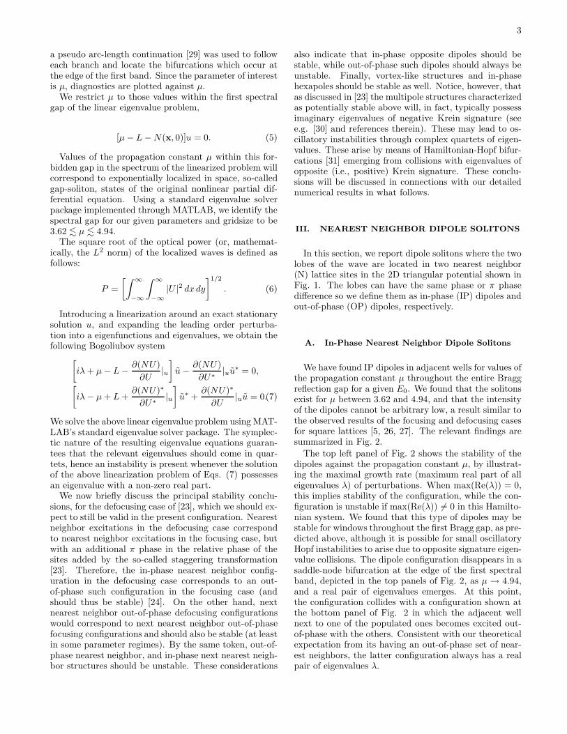
FIG. 14: The same dynamical evolution figure as Fig. 3, butfor the out-of-phase hexapole depicted in the bottom panel ofFig. 12. Depicted is the isosurface of height 0.1.

3.5 4 4.5 50

0.1

0.2

0.3

0.4

max

(Re(

λ))

µ3.5 4 4.5 5

0

5

10

15

20

P

µ

x

y

−50 0 50

−60

−40

−20

0

20

40

60

0

0.2

0.4

0.6

−1 0 1

x 10−3

−1

−0.5

0

0.5

1

λr

λ i

x

y

−50 0 50

−60

−40

−20

0

20

40

60

−0.6

−0.4

−0.2

0

0.2

0.4

0.6

−0.2 0 0.2

−1

−0.5

0

0.5

1

λr

λ i

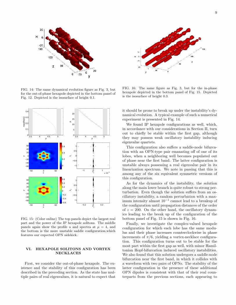
FIG. 15: (Color online) The top panels depict the largest realpart and the power of the IP hexapole solitons. The middlepanels again show the profile u and spectra at µ = 4, andthe bottom is the more unstable saddle configuration,whichfeatures our expected OPN sidekick.

VI. HEXAPOLE SOLITONS AND VORTEX

NECKLACES

First, we consider the out-of-phase hexapole. The ex-istence and the stability of this configuration has beendescribed in the preceding section. As the state has mul-tiple pairs of real eigenvalues, it is natural to expect that

FIG. 16: The same figure as Fig. 3, but for the in-phasehexapole depicted in the bottom panel of Fig. 15. Depictedis the isosurface of height 0.3.

it should be prone to break up under the instability’s dy-namical evolution. A typical example of such a numericalexperiment is presented in Fig. 14.

We found IP hexapole configurations as well, which,in accordance with our considerations in Section II, turnout to chiefly be stable within the first gap, althoughthey may possess weak oscillatory instability inducingeigenvalue quartets.

This configuration also suffers a saddle-node bifurca-tion with an OPN-type pair emanating off of one of itslobes, when a neighboring well becomes populated outof phase near the first band. The latter configuration isunstable always possessing a real eigenvalue pair in itslinearization spectrum. We note in passing that this isamong any of the six equivalent symmetric versions ofthis configuration.

As for the dynamics of the instability, the solutionalong the main lower branch is quite robust to strong per-turbation. Even though the solution suffers from an os-cillatory instability, a random perturbation with a max-imum intensity almost 10−1 cannot lead to a breakup ofthe configuration until propagation distances of the orderof z = 200. On the other hand, the oscillatory dynam-ics leading to the break up of the configuration of thebottom panel of Fig. 15 is shown in Fig. 16.

Finally, we investigate the complex-valued hexapoleconfiguration for which each lobe has the same modu-lus and their phase increases counterclockwise in phaseincrements of π/6, yielding a vortex-necklace configura-tion. This configuration turns out to be stable for themost part within the first gap as well, with minor Hamil-tonian Hopf-bifurcation induced oscillatory instabilities.We also found that this solution undergoes a saddle-nodebifurcation near the first band, in which it collides witha waveform with two pairs of OPNs. The stability of thelatter configuration in the presence of these additionalOPN dipoles is consistent with that of their real coun-terparts from the previous sections, each appearing to

10

3.5 4 4.5 50

0.1

0.2

0.3

0.4

max

(Re(

λ))

µ3.5 4 4.5 5

0

5

10

15

20

P

µ

x

y

−50 0 50

−60

−40

−20

0

20

40

60

0.05

0.1

0.15

0.2

−0.01−0.005 0 0.005 0.01

−1.5

−1

−0.5

0

0.5

1

1.5

λr

λ i

x

y

−50 0 50

−60

−40

−20

0

20

40

60

−0.3

−0.2

−0.1

0

0.1

0.2

0.3

x

y

−50 0 50

−60

−40

−20

0

20

40

60

−0.4

−0.2

0

0.2

0.4

x

y

−50 0 50

−60

−40

−20

0

20

40

60

−3

−2

−1

0

1

2

3

−50 0 50

−60

−40

−20

0

20

40

60

0.05

0.1

0.15

0.2

−0.2 −0.1 0 0.1 0.2

−1.5

−1

−0.5

0

0.5

1

1.5

λr

λ i

−50 0 50

−60

−40

−20

0

20

40

60

−0.3

−0.2

−0.1

0

0.1

0.2

0.3

−50 0 50

−60

−40

−20

0

20

40

60

−0.4

−0.2

0

0.2

0.4

−50 0 50

−60

−40

−20

0

20

40

60

−3

−2

−1

0

1

2

3

FIG. 17: (Color online) The top panels depict the largest real part and the power of the vortex necklace hexapole configuration.The second row depicts the modulus of the solution and corresponding spectrum when µ = 4.6. The third row illustratesthe real and imaginary components of the field and the phase (from left to right). The fourth and fifth rows show the sameproperties as the second and third but for the unstable eight-site configuration of the dashed line in the top panels.

11

FIG. 18: The same figure as Fig. 3, but for the vortex neck-lace with eight lobes depicted in the bottom panel of Fig. 17.Depicted is the isosurface of height 0.1.

contribute one real pair, rendering the relevant configu-ration quite unstable.

Similar to the case of in-phase hexapoles, even thoughvortex necklaces may be unstable, they are quite robustto perturbation, given the weak nature of the relevantoscillatory instabilities. We therefore only depict the dy-namics of the solutions which have eight lobes as shownin the fourth and fifth row panels of Fig. 17. The typicalevolution of this state is shown in Fig. 18, showcasingthe oscillatory breakup of this structure into one with asmaller number of lobes.

VII. CONCLUSIONS

In this communication, we examined in detail theo-retically and numerically the existence, stability and dy-namics of multipole lattice solitons excited with a sat-urable defocusing photorefractive nonlinearity in a tri-angular geometry. We have obtained a wide array ofrelevant structures, including different types of dipolesand hexapoles, as well as vortices. For the dipole con-figurations we examined the different possible phase con-figurations (in phase, and out phase profiles), as well ascases where the excited sites are separated by 0, 1, or2 intermediate lattices sites. For hexapoles, we exam-ined in phase and out of phase, and we also studied themonotonic increasing phase of a discrete vortex necklace.

We have found good agreement with the general guide-

lines, explained in section II, stemming from the theoret-ical analysis of the discrete model. This intuition led tothe illustration of a wide variety of potentially stable so-lutions (although they may incur oscillatory instabilities)such as the in phase, nearest neighbor dipole, the out ofphase, next nearest neighbor dipole, and the in phaseopposite dipole. We have also identified those solutionsincluding e.g., the out of phase nearest neighbor, in phasenext-nearest neighbor, and out of phase opposite dipoleswhich are typically unstable due to exponential instabili-ties and real eigenvalues. By the same considerations, thein-phase hexapole was proposed and was indeed found tobe typically stable, while the out-of-phase one was pre-dicted and observed to be quite unstable, due to multiplereal eigenvalue pairs. Finally, we have seen that the dis-crete vortex structure is also potentially stable.

Furthermore, we have also identified an interesting setof bifurcations that are associated with the paramet-ric continuation and termination of some of the abovebranches. The dynamical instabilities encountered in thepresent work have been monitored through direct inte-gration of the relevant dynamical equation. The result ofevolution in every case involved oscillations between theoriginal configuration and one with fewer sites which ismore stable, such as a single site solitary wave, and some-times degeneration to such a configuration. Solutionswith smaller power tend to decay into a single site soli-tary wave for certain solutions investigated, while thosewith larger power tend to oscillate. This connection isbeyond the scope of the present work, but is currentlybeing investigated further.

Since the framework of defocusing equations has beenstudied far less extensively than their focusing counter-parts, it would be particularly interesting to extend thepresent considerations to other structures. Perhaps themost interesting example would be the study of multiplecharge vortices in this context which would be an inter-esting endeavor both from a theoretical, as well as froman experimental point of view. Such studies are currentlyin progress and will be reported in future publications.

Acknowledgements. PGK acknowledges supportfrom NSF-DMS-0505663, NSF-DMS-0619492 and NSF-CAREER. W. Krolikowski is gratefully acknowledged fornumerous informative discussions on the theme of thiswork.

[1] N.K. Efremidis, S. Sears, D. N. Christodoulides, J. W.Fleischer, and M. Segev Phys. Rev. E 66, 46602 (2002).

[2] J.W. Fleischer, M. Segev, N.K. Efremidis and D.N.Christodoulides, Nature 422, 147 (2003); J.W. Fleis-cher, T. Carmon, M. Segev, N.K. Efremidis and D.N.Christodoulides, Phys. Rev. Lett. 90, 23902 (2003).

[3] D. Neshev, E. Ostrovskaya, Yu.S. Kivshar and W. Kro-

likowski, Opt. Lett. 28, 710 (2003).[4] H. Martin, E.D. Eugenieva, Z. Chen and D.N.

Christodoulides, Phys. Rev. Lett. 92, 123902 (2004).[5] J. Yang, I. Makasyuk, A. Bezryadina, and Z. Chen, Opt.

Lett. 29, 1662 (2004).[6] J. Yang, I. Makasyuk, P. G. Kevrekidis, H. Martin, B. A.

Malomed, D. J. Frantzeskakis, and Zhigang Chen, Phys.

12

Rev. Lett. 94, 113902 (2005).[7] D. Neshev, Yu. S. Kivshar, H. Martin, and Z. Chen, Opt.

Lett. 29, 486-488 (2004).[8] X. Wang, Z. Chen, and P. G. Kevrekidis, Phys. Rev. Lett.

96, 083904 (2006).[9] D. N. Neshev, T.J. Alexander, E.A. Ostrovskaya, Yu.S.

Kivshar, H. Martin, I. Makasyuk and Z. Chen, Phys.Rev. Lett. 92, 123903 (2004); J. W. Fleischer, G. Bartal,O. Cohen, O. Manela, M. Segev, J. Hudock, and D.N.Christodoulides Phys. Rev. Lett. 92, 123904 (2004).

[10] B. Freedman, G. Bartal, M. Segev, R. Lifshitz, D.N.Christodoulides and J.W. Fleischer, Nature 440, 1166(2006).

[11] T. Schwartz, G. Bartal, S. Fishman and M. Segev, Nature446, 52 (2007).

[12] D. N. Christodoulides, F. Lederer, and Y. Silberberg, Na-ture 424, 817 (2003); A. A. Sukhorukov, Y. S. Kivshar,H. S. Eisenberg, and Y. Silberberg, IEEE J. Quant. Elect.39, 31 (2003).

[13] S. Aubry, Physica 103D, 201 (1997); S. Flach and C. R.Willis, Phys. Rep. 295, 181 (1998); D. K. Campbell, S.Flach, and Y. S. Kivshar, Phys. Today, January 2004, p.43.

[14] V. A. Brazhnyi and V. V. Konotop, Mod. Phys. Lett. B18, 627 (2004); P. G. Kevrekidis and D. J. Frantzeskakis,Mod. Phys. Lett. B 18, 173 (2004).

[15] O. Morsch and M. Oberthaler, Rev. Mod. Phys. 78, 179(2006).

[16] P.G. Kevrekidis, B.A. Malomed and Yu.B. Gaididei,Phys. Rev. E 66, 016609 (2002).

[17] M.J. Ablowitz, B. Ilan, E. Schonbrun and R. Piestun,Phys. Rev. E 74, 035601 (2006).

[18] B. Freedmna, G. Bartal, M. Segev, R. Lifshitz, D.N.Christodoulides and J.W. Fleischer, Nature (London)440, 1166 (2006).

[19] C.R. Rosberg, D.N. Neshev, A.A. Sukhorukov, W. Kro-likowski and Yu.S. Kivshar, Opt. Lett. 32, 397 (2007).

[20] T.J. Alexander, A.S. Desyatnikov and Yu.S. Kivshar,Opt. Lett. 32, 1293 (2007).

[21] O. Peleg, G. Bartal, B. Freedman, O. Manela, M.Segev,and D. Christodoulides, Phys. Rev. Lett. 98, 103901(2007).

[22] L. Tang, C. Lou, X. Wang, D. Song, X. Chen, J. Xu,Z. Chen, H. Susanto, K. Law and P.G. Kevrekidis, Opt.Lett. 32, 3011 (2007).

[23] P.G. Kevrekidis, H. Susanto and Z. Chen, Phys. Rev. E74, 066606 (2006).

[24] P.G. Kevrekidis, K.Ø. Rasmussen and A.R. Bishop, Int.J. Mod. Phys. B 15, 2833 (2001); D.E. Pelinovsky, P.G.Kevrekidis and D.J. Frantzeskakis, Physica D 212, 1(2005); ibid 212, 20 (2005).

[25] J. Yang, New J. Phys. 6, 47 (2004).[26] J. Yang, A. Bezryadina, I. Makasyuk and Z. Chen, Stud.

Appl. Math. 113, 389 (2004).[27] H. Susanto, K. Law, P.G. Kevrekidis, L. Tang, C. Lou,

X. Wang and Z. Chen, Dipole and quadrupole solitonsin two-dimensional defocusing photonic lattices. preprint(2007).

[28] C. T. Kelley, Solving Nonlinear Equations with Newtons

Method, no. 1 in Fundamentals of Algorithms, SIAM,Philadelphia, 2003.

[29] E. Doedel. International Journal of Bifurcation andChaos. 7(9):2127-2143, 1997.

[30] T. Kapitula, P.G. Kevrekidis, B. Sandstede, Physica D195 263 (2004).

[31] J.-C. van der Meer, Nonlinearity 3, 1041 (1990).[32] D. Pelinovsky, A.A. Sukhorukov, and Yu.S. Kivshar,

Phys. Rev. E 70, 036618 (2004).[33] Z. Shi and J. Yang, Phys. Rev. E 75, 056602 (2007).