
Chern–Simons vortices in the Gudnason model
39
arXiv:1307.6951v1 [math.AP] 26 Jul 2013 Chern–Simons Vortices in the Gudnason Model Xiaosen Han Institute of Contemporary Mathematics School of Mathematics Henan University Kaifeng, Henan 475004, PR China Chang-Shou Lin Department of Mathematics National Taiwan University Taipei, Taiwan 10617, ROC Gabriella Tarantello Dipartimento di Matematica Unversit`a di Roma “Tor Vergata” Via della Ricerca Scientifica 00133 Rome, Italy Yisong Yang Department of Mathematics Polytechnic Institute of New York University Brooklyn, New York 11201, USA Abstract We present a series of existence theorems for multiple vortex solutions in the Gudnason model of the N = 2 supersymmetric field theory where non-Abelian gauge fields are governed by the pure Chern–Simons dynamics at dual levels and realized as the solutions of a system of elliptic equations with exponential nonlinearity over two-dimensional domains. In the full plane situation, our method utilizes a minimization approach, and in the doubly periodic situation, we employ an-inequality constrained minimization approach. In the latter case, we also obtain sufficient conditions under which we show that there exist at least two gauge-distinct solutions for any prescribed distribution of vortices. In other words, there are distinct solutions with identical vortex distribution, energy, and electric and magnetic charges. 1 Introduction The classical Abelian Higgs model defined by the Lagrangian action density L AH = − 1 4 F μ F μν + 1 2 D μ φ D μ φ − λ 8 (|φ| 2 − 1) 2 , (1.1) 1
-
Upload
independent -
Category
Documents
-
view
6 -
download
0
Transcript of Chern–Simons vortices in the Gudnason model

arX
iv:1
307.
6951
v1 [
mat
h.A
P] 2
6 Ju
l 201
3
Chern–Simons Vortices in the Gudnason Model
Xiaosen Han
Institute of Contemporary Mathematics
School of Mathematics
Henan University
Kaifeng, Henan 475004, PR China
Chang-Shou Lin
Department of Mathematics
National Taiwan University
Taipei, Taiwan 10617, ROC
Gabriella Tarantello
Dipartimento di Matematica
Unversita di Roma “Tor Vergata”
Via della Ricerca Scientifica
00133 Rome, Italy
Yisong Yang
Department of Mathematics
Polytechnic Institute of New York University
Brooklyn, New York 11201, USA
Abstract
We present a series of existence theorems for multiple vortex solutions in the Gudnason
model of the N = 2 supersymmetric field theory where non-Abelian gauge fields are governed
by the pure Chern–Simons dynamics at dual levels and realized as the solutions of a system of
elliptic equations with exponential nonlinearity over two-dimensional domains. In the full plane
situation, our method utilizes a minimization approach, and in the doubly periodic situation,
we employ an-inequality constrained minimization approach. In the latter case, we also obtain
sufficient conditions under which we show that there exist at least two gauge-distinct solutions
for any prescribed distribution of vortices. In other words, there are distinct solutions with
identical vortex distribution, energy, and electric and magnetic charges.
1 Introduction
The classical Abelian Higgs model defined by the Lagrangian action density
LAH = −1
4FµF
µν +1
2DµφDµφ− λ
8(|φ|2 − 1)2, (1.1)
1

is of foundational importance in theoretical physics. Here φ is a complex-valued scalar field called
the Higgs field, Fµν = ∂µAν −∂νAµ the electromagnetic field strength generated from a real-valued
gauge field, Aµ, Dµφ = ∂µφ − iAµφ the gauge-covariant derivative, λ > 0 a coupling parameter,
µ, ν = 0, 1, 2, 3 are the (3 + 1)-dimensional Minskowski spacetime coordinate indices, and the
metrics (gµν) = (gµν) = diag(1,−1,−1,−1) are used to raise or lower indices. For example, in
quantum field theory, the model provides a mathematically simplest thought-laboratory allowing
various fundamental concepts such as spontaneous symmetry-breaking, the onset and annihilation
of the Goldstone particles, and the Higgs mechanism to be formulated and explored [13, 35, 53].
Phenomenologically, the model in its static limit and temporal gauge A0 = 0 is the celebrated
Ginzburg–Landau theory [26] for superconductivity. In two spatial dimensions, topological defects
in the form of the Abrikosov vortices [1,21] can be generated from the model which, when coupled
with the Einstein equations, provide indispensable structures, known as cosmic strings, giving
rise to centers of curvature concentrations in spacetime and hence forming the seeds for matter
accretion in the early universe [68,71,72]. On the other hand, however, a statement known as the
Julia–Zee theorem [41,62] says that the static solutions of the equations of motion of (1.1) as well
as of that of the general non-Abelian Yang–Mills–Higgs model, in two-spatial dimensions and of
finite energy, must stay in the temporal gauge, A0 = 0. In other words, vortices of the Yang–
Mills–Higgs model, Abelian or non-Abelian, do not carry electric charge and can only be purely
magnetic. Nevertheless, electrically and magnetically charged vortices, called dyonic vortices, are
needed in many areas of applications such as high-temperature superconductivity [43, 47], the
Bose–Einstein condensates [36, 42], the quantum Hall effect [59], optics [9], and superfluids [56].
Therefore, it will be important to modify the classical Yang–Higgs–Higgs theory so that dyonic
vortices are accommodated. In a series of pioneering studies, Jackiw and Templeton [38], Schonfeld
[54], Deser, Jackiw, and Templeton [19,20], Paul and Khare [51], de Vega and Schaposnik [66,67],
and Kumar and Khare [44] developed a modified Yang–Mills–Higgs theory in which the Chern–
Simons topological terms [17,18] are implemented into the action density. Although these terms fail
to be gauge-invariant locally, they preserve gauge-invariance globally and thus render the theory
the same gauge invariance as in the Yang–Mills–Higgs theory. More importantly, the presence
of the Chern–Simons terms make the coexistence of electric and magnetic charges a necessity.
Mathematically, however, the presence of the Chern–Simons terms and the nontrivial temporal
component of the gauge field leads us to face a much more complicated form of the equations of
motion and an existence theory for radially symmetric solutions has only been obtained rather
recently [15]. This difficulty motivated people to explore possible BPS (after the seminal studies
of Bogomol’nyi [10] and Prasad and Sommerfield [52]) reductions of the problem and brought into
light the works of Hong, Kim, and Pac [33] and Jackiw and Weinberg [39], which sparked a great
development of the subject of construction of the Chern–Simons–Higgs vortex solutions up to today.
In their approach, it may be understood that the initial Lagrangian action density to be modified
is simply that of the Abelian Higgs model, with the addition of a Chern–Simons term controlled
by a coupling parameter κ, which may be written as
LMCSH = − 1
4e2FµνF
µν − κ
4ǫµνρAµFνρ +DµφDµφ− V (|φ|2), (1.2)
where e > 0 denotes a coupling parameter imposed on the Maxwell kinetic density term and V is
the Higgs potential density function, as in [51, 66]. Since in (1.2) both the Maxwell and Chern–
Simons terms are present, the model is referred to as the Maxwell–Chern–Simons–Higgs model. In
2

the limit e→ ∞, the Maxwell term is switched off and the model (1.2) becomes
LACSH = −κ4ǫµνρAµFνρ +DµφDµφ− V (|φ|2), (1.3)
which is known as the Abelian Chern–Simons–Higgs model [33,39] in which the gauge field dynamics
is governed solely by the Chern–Simons term. It is shown in [33,39] that, when the Higgs potential
function V is chosen to be
V (|φ|2) = 1
κ2|φ|2(1− |φ|2)2, (1.4)
which is analogous with the critical choice λ = 1 for (1.1) studied in [40], the equations of motion
of (1.3) may be reduced into the BPS system
D1φ+ iD2φ = 0, F12 =2
κ2|φ|2(1− |φ|2). (1.5)
The multiple vortex solutions, realizing a prescribed distribution of vortices located at p1, . . . , pnand carrying the total electric and magnetic charges, Qe and Qm, given by
Qe = κQm, Qm =
∫
F12 dx = 2πn, (1.6)
may be constructed in terms of the variable u = |φ|2 via solving the master equation [33,39]
∆u = αeu(eu − 1) + 4π
n∑
s=1
δps(x), (1.7)
where α = 4κ2, whose structure has been shown [64, 74] to be much richer and more challenging
than that of the classical Abelian Higgs model. For example, in contrast to the Abelian Higgs
model (1.1) where the solution of finite energy realizing any prescribed distribution of vortices is
unique [40, 65, 70], the solutions in the Abelian Chern–Simons–Higgs model are not unique and
further categorized [22, 34, 37] into topological and non-topological solutions, which have led to a
rapid development of analytic methods and the harvest of a rich vista of results [11,12,14,16,60,61]
regarding issues such as existence, uniqueness, nonexistence, asymptotic properties, approximation,
etc., of the solutions.
The purpose of the present article is to develop an existence theory for non-Abelian Chern–
Simon–Higgs vortices in the Gudnason model [27, 28]. Historically, after the formulation of the
Abelian Chern–Simons–Higgs model in [33, 39], a great deal of activities quickly evolved around
developing [23] and analyzing [45,48,73] non-Abelian extensions of the model, both non-relativistic
and relativistic. What distinguish the Gudnason model [27, 28] from the classical non-Abelian
Chern–Simons–Higgs models [23, 66, 67] are that the former may be derived in a supersymmetric
gauge field theory framework as those in the study of monopole confinement mechanism [5,31,32,
46,57,58] and that a kind of bi-level Chern–Simons dynamics is present as in the Bagger–Lambert–
Gustavsson theory [6–8, 29] and the Aharony–Bergman–Jafferis–Maldacena theory [2] to govern
gauge-field kinematics. These studies have prompted a great amount of research activities over the
past few years and the nonlinear partial differential equation problems unearthed offer truly rich
opportunities for analysts in exploring new techniques and ideas.
We shall present two types of results. The first type concerns the existence of solutions over
the full plane subject to the boundary behavior corresponding to the asymptotic vacuum state
with a completely broken symmetry [27, 28]. Our method is based on a variational reformulation
3

of the problem and a coercive minimization approach. The second type concerns the existence,
nonexistence, and multiplicity of solutions over a doubly periodic domain. The main difficulty
we encounter here is the constraint problem which makes it hard to develop a general variational
method as in the full plane situation where there is no constraint to tackle. In this situation
we compromise to solve the system in the special case with two equations. Although this case
is limited, the results are rich and structures are challenging. Here we extend the inequality-
constrained techniques [11,48,63] to resolve the equality-constraint difficulty and obtain existence
and multiplicity results for solutions.
A brief outline of the rest of the paper is as follows. In the next section, we first review the
Gudnason model [27, 28] and the associated non-Abelian vortex equations, also called the master
equations [27, 28], to be studied in this paper. In the following section, we reduce the master
equations into a system of nonlinear equations to be analyzed and state our main existence theorems
regarding the solutions. The subsequent sections are then devoted to the proofs of these theorems
by developing and utilizing variational techniques. In the last section, we briefly summarize and
comment on our results.
2 The Gudnason model
Consider the standard Minkowski spacetime R2,1 of signature (+ − −) and use µ, ν = 0, 1, 2 to
denote the temporal and spatial coordinate indices. The Gudnason model [27] is formulated as
an N = 2 supersymmetric Yang–Mills–Chern–Simons–Higgs theory with the general gauge group
G = U(1) × G′ where G′ is a non-Abelian simple Lie group represented by matrices. As in [27],
use the index a = 1, . . . ,dim(G′) to label the non-Abelian gauge group generators and the index
0 the Abelian one, U(1). Then the gauge potential Aµ taking values in the Lie algebra of the
group G may be written as Aµ = Aαµtα where Aαµ are real-valued vector fields and tα (α = 0, a) the
generators of G which are normalized to satisfy
t0 =1√2N
, Tr(tatb) =1
2δab, (2.8)
where N is the dimension of the fundamental representation space of G′. The gauge field strength
tensor Fµν is then given by
Fµν = ∂µAν − ∂νAµ + i[Aµ, Aν ]. (2.9)
Use φ to denote the Higgs scalar field in the adjoint representation of G and the N × Nf matrix
H to contain Nf-flavor matter (quark) fields in the fundamental representation of G. Then their
gauge-covariant derivatives are
Dµφ = ∂µφ+ i[Aµ, φ], DµH = ∂µH + iAµH. (2.10)
With this preparation, the Lagrangian action density of the Yang–Mills–Chern–Simons–Higgs the-
ory of the Gudnason model [27], omitting the Fermion part, is written as
LYMCSH = − 1
4g2(F aµν)
2 − 1
4e2(F 0
µν)2 − µ
8πǫµνρ
(
Aaµ∂νAaρ −
1
3fabcAaµA
bνA
cρ
)
− κ
8πǫµνρA0
µ∂νA0ρ
+1
2g2(Dµφ
a)2 +1
2e2(∂µφ
0)2 +Tr(DµH)(DµH)† − Tr|φH −Hm|2
−g2
2
(
Tr(HH†ta)− µ
4πφa)2
− e2
2
(
Tr(HH†t0)− κ
4πφ0 − ξ√
2N
)2
, (2.11)
4
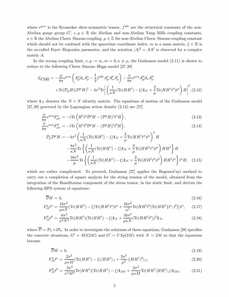
where ǫµνν is the Kronecker skew-symmetric tensor, fabc are the structural constants of the non-
Abelian gauge group G′, e, g ∈ R the Abelian and non-Abelian Yang–Mills coupling constants,
κ ∈ R the Abelian Chern–Simons coupling, µ ∈ Z the non-Abelian Chern–Simons coupling constant
which should not be confused with the spacetime coordinate index, m is a mass matrix, ξ ∈ R is
the so-called Fayet–Iliopoulos parameter, and the notation |A|2 = AA† is observed for a complex
matrix A.
In the strong coupling limit, e, g → ∞,m = 0, κ 6= µ, the Gudnason model (2.11) is shown to
reduce to the following Chern–Simons–Higgs model [27,28]
LCSH = − µ
8πǫµνρ
(
Aaµ∂νAaρ −
1
3fabcAaµA
bνA
cρ
)
− κ
8πǫµνρA0
µ∂νA0ρ
+Tr(DµH)(DµH)† − 4π2Tr
∣
∣
∣
∣
(
1
κN(Tr(HH†)− ξ)1N +
2
µTr(HH†ta)ta
)
H
∣
∣
∣
∣
2
,(2.12)
where 1N denotes the N × N identity matrix. The equations of motion of the Gudnason model
[27,28] governed by the Lagrangian action density (2.12) are [27]
µ
8πǫµνρF aµν = −iTr
(
H†taDρH − (DρH)†taH)
, (2.13)
κ
8πǫµνρF 0
µν = −iTr(
H†t0DρH − (DρH)†t0H)
, (2.14)
DµDµH = −4π2(
1
κN(Tr(HH†)− ξ)1N +
2
µTr(HH†ta)ta
)2
H
−8π2
κNTr
(
1
κN(Tr(HH†)− ξ)1N +
2
µTr(HH†ta)ta
)
HH†
H
−16π2
µTr
(
1
κN(Tr(HH†)− ξ)1N +
2
µTr(HH†tb)tb
)
HH†ta
taH, (2.15)
which are rather complicated. To proceed, Gudnason [27] applies the Bogomol’nyi method to
carry out a completion of square analysis for the string tension of the model, obtained from the
integration of the Hamiltonian component of the stress tensor, in the static limit, and derives the
following BPS system of equations:
DH = 0, (2.16)
F a12ta =
16π2
µκN(Tr(HH†)− ξ)Tr(HH†ta)ta +
16π2
µ2Tr(HH†tb)Tr(HH†ta, tb)ta, (2.17)
F 012t
0 =8π2
κ2N2Tr(HH†)(Tr(HH†)− ξ)1N +
16π2
µκN(Tr(HH†ta))21N , (2.18)
where D = D1+iD2. In order to investigate the solutions of these equations, Gudnason [28] specifies
the concrete situations, G′ = SO(2M) and G′ = USp(2M) with N = 2M so that the equations
become
DH = 0, (2.19)
F a12ta =
2π2
µκM(Tr(HH†)− ξ)〈HH†〉J +
2π2
µ2〈(HH†)2〉J , (2.20)
F 012t
0 =2π2
κ2M2Tr(HH†)(Tr(HH†)− ξ)12M +
2π2
µκMTr(HH†〈HH†〉J)12M , (2.21)
5

in which 〈A〉J = A− J†AtJ for a 2M × 2M matrix with
J =
(
0 1M
ǫ1M 0
)
, ǫ = ±1 depending on whether G′ = SO(2M) or USp(2M). (2.22)
Then, choosing H0 as a suitable background matrix realizing a prescribed distribution of vortices
and using a moduli matrix ansatz of the form H = S−1H0, S = sS′, which splits the variables into
the Abelian one ω = |s|2 and the non-Abelian one Ω′ = S′(S′)†, so that Ω = SS† = ωΩ′, the BPS
equations (2.19)–(2.21) are shown to become the so-called master equations [28]
∂(Ω′∂Ω′−1) =π2
µκM(Tr(Ω0Ω
−1)− ξ)〈Ω0Ω−1〉J +
π2
µ2〈(Ω0Ω
−1)2〉J , (2.23)
∂∂ lnω = − π2
κ2M2Tr(Ω0Ω
−1)(Tr(Ω0Ω−1)− ξ)− π2
µκMTr(Ω0Ω
−1〈Ω0Ω−1〉J), (2.24)
where ∂ = ∂1 + i∂2.
To describe multiple vortices by the master equations (2.23)–(2.24), we take as in [27, 28] the
moduli matrix H0(z) of the form
H0(z) =
M∏
i=1
ni∏
s=1
(z − zi,s)D0(z),
where
D0(z) = diag
n1∏
s=1
(z − z1,s), . . . ,
nM∏
s=1
(z − zM,s),
n1∏
s=1
(z − z1,s)−1, . . . ,
nM∏
s=1
(z − zM,s)−1
,
and zi,s are prescribed points on the complex plane, s = 1, . . . , ni, i = 1, . . . ,M ; ni are nonnegative
integers, i = 1, . . . ,M . We easily see that
HT0 (z)JH0(z) =
M∏
i=1
ni∏
s=1
(z − zi,s)J,
det (H0(z)) =
(
M∏
i=1
ni∏
s=1
(z − zi,s)
)2M
,
Ω0 = H0(z)H0(z)† =
M∏
i=1
ni∏
s=1
|z − zi,s|2D0(z)†D0(z).
With the further ansatz
Ω′ = diag(eχ1 , . . . , eχM , e−χ1 , . . . , e−χM ), ω = eψ, (2.25)
where χ1, . . . , χM , ψ are real-valued functions, and a direct computation, the equations (2.23)–(2.24)
6

read [28]:
∂∂χj = − π2
µκM
(
M∏
k=1
nk∏
s=1
|z − zk,s|2M∑
i=1
[
ni∏
s=1
|z − zi,s|2e−ψ−χi +
ni∏
s=1
|z − zi,s|−2e−ψ+χi
]
− ξ
)
×M∏
k=1
nk∏
s=1
|z − zk,s|2( nj∏
s=1
|z − zj,s|2e−ψ−χj −nj∏
s=1
|z − zj,s|2e−ψ+χj
)
−π2
µ2
M∏
k=1
nk∏
s=1
|z − zk,s|4( nj∏
s=1
|z − zj,s|4e−2ψ−2χj −nj∏
s=1
|z − zj,s|−4e−2ψ+2χj
)
,
j = 1, . . . ,M, (2.26)
∂∂ψ = − π2
κ2M2
(
M∏
k=1
nk∏
s=1
|z − zk,s|2M∑
i=1
[
ni∏
s=1
|z − zi,s|2e−ψ−χi +
ni∏
s=1
|z − zi,s|−2e−ψ+χi
]
− ξ
)
×M∏
k=1
nk∏
s=1
|z − zk,s|2M∑
j=1
( nj∏
s=1
|z − zj,s|2e−ψ−χj +
nj∏
s=1
|z − zj,s|−2e−ψ+χj
)
− π2
µκM
M∑
i=1
nk∏
s=1
|z − zk,s|4M∑
i=1
(
ni∏
s=1
|z − zi,s|2e−ψ−χi −ni∏
s=1
|z − zi,s|−2e−ψ+χi
)2
. (2.27)
These are the master equations which govern the multiple vortex solutions of the non-Abelian
Chern–Simons–Higgs model of Gudnason [27, 28]. Below we aim to establish a series of existence
theorems for the solutions of these equations over the full plane and over doubly periodic cell
domains.
3 Non-Abelian vortex equations and existence theorems
We consider the non-Abelian Chern–Simons–Higgs vortex equations (2.26)–(2.27). With
u = −ψ +
M∑
i=1
ni∑
s=1
ln |z − zi,s|2, uj = −χj +nj∑
s=1
ln |z − zj,s|2, j = 1, . . . ,M,
we see that
eu =
M∏
i=1
ni∏
s=1
|z − zi,s|2e−ψ, euj =
nj∏
s=1
|z − zj,s|2e−χj , j = 1, . . . ,M.
Then the equations (2.26)–(2.27) become
∆u =α2
M2
(
M∑
i=1
[
eu+ui + eu−ui]
− ξ
)
M∑
j=1
[
eu+uj + eu−uj]
+αβ
M
M∑
i=1
(eu+ui − eu−ui)2 + 4π
M∑
i=1
ni∑
s=1
δpi,s(x), (3.1)
∆uj =αβ
M
(
M∑
i=1
[
eu+ui + eu−ui]
− ξ
)
(eu+uj − eu−uj)
+β2(e2u+2uj − e2u−2uj ) + 4π
nj∑
s=1
δpj,s(x), j = 1, . . . ,M, (3.2)
7

where we set α = πκ, β = π
µ, pi,s = zi,s, i = 1, . . . ,M. When M = 1 such equations were first
obtained in [27]. It will be convenient to take the rescaled parameters and translated variables
αξ
2M7→ α, β
ξ
2M7→ β, u 7→ u+ ln
ξ
2M, uj 7→ uj, j = 1, . . . ,M.
Then the equations (3.1) and (3.2) are renormalized into the form
∆u =α2
M2
(
M∑
i=1
[
eu+ui + eu−ui − 2]
)
M∑
j=1
[
eu+uj + eu−uj]
+αβ
M
M∑
i=1
(
eu+ui − eu−ui)2
+ 4π
M∑
i=1
ni∑
s=1
δpi,s(x), (3.3)
∆uj =αβ
M
(
M∑
i=1
[
eu+ui + eu−ui − 2]
)
(
eu+uj − eu−uj)
+β2(
e2u+2uj − e2u−2uj)
+ 4π
nj∑
s=1
δpj,s(x), j = 1, . . . ,M. (3.4)
It will be interesting at this spot to compare the classical Abelian Chern–Simons–Higgs vortex
equation (1.7) with the above system of non-Abelian vortex equations, (3.3) and (3.4), in the
Gudnason model [27,28], which will be our focus in the present work.
We will consider the equations (3.3)–(3.4) in two cases. In the first case we study the problem
(3.3)–(3.4) over the full plane R2 with the topological boundary conditions
u→ 0, uj → 0 as |x| → ∞, j = 1, . . . ,M, (3.5)
realizing the asymptotic vacuum state with completely broken symmetry [27,28].
We have the following existence theorem.
Theorem 3.1 For any sets of points
Zi = pi,1, . . . , pi,ni ⊂ R
2, i = 1, . . . ,M, (3.6)
and the parameters α, β > 0, M ≥ 1, the system of nonlinear elliptic equations (3.3)–(3.4) subject
to the boundary condition (3.5) admits a solution over R2 which possesses the quantized integrals
α2
M2
∫
R2
(
M∑
i=1
[
eu+ui + eu−ui − 2]
)
M∑
j=1
[
eu+uj + eu−uj]
dx
+αβ
M
M∑
i=1
∫
R2
(
eu+ui − eu−ui)2
dx = −4π
M∑
i=1
ni, (3.7)
αβ
M
∫
R2
M∑
j=1
[
eu+uj + eu−uj − 2]
(
eu+ui − eu−ui)
dx
+β2∫
R2
(
e2u+2ui − e2u−2ui)
dx = −4πni, i = 1, . . . ,M. (3.8)
8

Furthermore the boundary condition (3.5) is realized exponentially fast so that there hold the fol-
lowing asymptotic estimates near infinity:
u2 +M∑
i=1
u2i = O(e−m(1−ε)|x|), |∇u|2 +M∑
i=1
|∇ui|2 = O(e−m(1−ε)|x|), (3.9)
where m = 2√2minα, β and ε ∈ (0, 1) is an arbitrarily small parameter.
In the second case we consider the equations (3.3)–(3.4) over a doubly periodic domain Ω with
M = 1. That is, in this case we study a 2 × 2 version of (3.3)–(3.4). For convenience we rewrite
the system (3.3)–(3.4) with M = 1 as follows
∆U = α2(
eU+V + eU−V ) (eU+V + eU−V − 2)
+ αβ(
eU+V − eU−V )2 + 4π
n∑
j=1
δpj (x), (3.10)
∆V = αβ(
eU+V − eU−V ) (eU+V + eU−V − 2)
+ β2(
e2U+2V − e2U−2V)
+ 4π
n∑
j=1
δpj (x). (3.11)
We have the following existence results.
Theorem 3.2 Let Ω be a doubly periodic domain in R2 and p1, . . . , pn ∈ Ω which need not to be
distinct with repeated p’s counting for multiplicities. Assume that β > α > 0.
1. If the equations (3.10) and (3.11) have a solution, then there holds the condition
8πn ≤ αβ|Ω|. (3.12)
2. Every solution (U, V ) of (3.10) and (3.11) satisfies
eU < 1, eU+V < 1, eU−V < 1. (3.13)
3. For any given constant σ > 1, assumeβ
α< σ. (3.14)
Then, there exist a positive constant Mσ such that when α > Mσ the equations (3.10) and
(3.11) admit at least two distinct solutions over Ω, one of which satisfies the behavior
eU+V → 1, eU−V → 1, as α→ +∞ (3.15)
pointwise a.e. in Ω. Furthermose, any solution (U, V ) of (3.10) and (3.11) possesses the
quantized integrals
α2
∫
Ω
(
eU+V + eU−V ) (eU+V + eU−V − 2)
dx+ αβ
∫
Ω
(
eU+V − eU−V )2 dx = −4πn, (3.16)
αβ
∫
Ω
(
eU+V − eU−V ) (eU+V + eU−V − 2)
dx+β2∫
Ω
(
e2U+2V − e2U−2V)
dx = −4πn. (3.17)
In Section 4, we establish Theorem 3.1 using a direct minimization method which extends
the techniques in [40, 65, 73, 74]. In Section 5, we prove Theorem 3.2 by utilizing and extending
an inequality-constrained variational method originally developed in [11] and further developed
in [49, 50, 63], and subsequently in [48] for a context that relates more to the situation considered
here. In this respect, see also [30].
9

4 Proof of Theorem 3.1
In this section we prove the existence of topological solutions for the equations (3.3)–(3.4).
Choosing the background functions
u0i (x) = −ni∑
s=1
ln(
1 + λ|x− pi,s|−2)
, λ > 0, i = 1, . . . ,M, (4.1)
which satisfy
∆u0i = −hi + 4π
ni∑
s=1
δpi,s , hi(x) = 4λ
ni∑
s=1
1
(λ+ |x− pi,s|2)2, (4.2)
we see that the new variables
u =
M∑
i=1
u0i + f, uj = u0j + fj, j = 1, . . . ,M, (4.3)
allow us to recast the equations (3.3)–(3.4) into
∆f =α2
M2
M∑
i=1
e
M∑
k=1
u0k+u0i+f+fi
+ e
M∑
k=1
u0k−u0i+f−fi − 2
M∑
j=1
e
M∑
k=1
u0k+u0j+f+fj
+ e
M∑
k=1
u0k−u0j+f−fj
+αβ
M
M∑
i=1
e
M∑
k=1
u0k+u0i+f+fi − e
M∑
k=1
u0k−u0i+f−fi
2
+
M∑
i=1
hi, (4.4)
∆fi =αβ
M
M∑
j=1
e
M∑
k=1
u0k+u0j+f+fj
+ e
M∑
k=1
u0k−u0j+f−fj − 2
e
M∑
k=1
u0k+u0i+f+fi − e
M∑
k=1
u0k−u0i+f−fi
+β2
e2
M∑
k=1
u0k+2u0i+2f+2fi − e
2M∑
k=1
u0k−2u0i+2f−2fi
+ hi, i = 1, . . . ,M. (4.5)
The topological boundary condition (3.5) becomes
f → 0, fi → 0 as |x| → ∞, i = 1, . . . ,M. (4.6)
It can be checked that the equations (4.4) and (4.5) are the Euler–Lagrange equations of the
functional
I(f, f1, . . . , fM )
=
∫
R2
dx
M
α|∇f |2 + 1
β
M∑
i=1
|∇fi|2 +M∑
i=1
α
M
e
M∑
k=1
u0k+u0i+f+fi
+ e
M∑
k=1
u0k−u0i+f−fi − 2
2
+β
e
M∑
k=1
u0k+u0i+f+fi − e
M∑
k=1
u0k−u0i+f−fi
2
+2M
α
M∑
i=1
fhi +2
β
M∑
i=1
fihi
. (4.7)
We consider the functional I over W 1,2(R2). Here and in what follows we use W 1,2(R2) to
denote the usual Sobolev space of scalar-valued or vector-valued functions. It is not difficult to
see that the functional I is continuous, differentiable and lower semi-continuous on W 1,2(R2). The
10

important thing is that we can show that the functional I is coercive and bounded from below over
W 1,2(R2), which will be carried out later. Then we can conclude that the functional I admits a
critical point (f, f1, . . . , fM ) ∈W 1,2(R2), which is a weak solution to the equations (4.4)–(4.5). By
the following inequality
‖ew − 1‖22 ≤ C exp(
C‖w‖2W 1,2(R2)
)
, ∀w ∈W 1,2(R2),
we see that the right hand side of the equations (4.4)–(4.5) belongs to L2(R2). Then using elliptic
L2-estimates and a bootstrap argument, we find that the solution (f, f1, . . . , fM ) is smooth. In
particular, (f, f1, . . . , fM ) lies inW 2,2(R2) which ensures that (f, f1, . . . , fM ) satisfies the boundary
condition (4.6). Then, in view of (4.3), we see that the problem consisting of the equations (3.3)
and (3.4) admits a solution (u, u1, . . . , uM ) satisfying the boundary condition (3.5).
We now establish the exponential decay estimates for the solution.
We first note that
eu+ui + eu−ui − 2 = (eu+ui − 1) + (eu−ui − 1) = eξ′
i(u+ ui) + eξ′′
i (u− ui)
= (eξ′
i + eξ′
i)u+ (eξ′
i − eξ′′
i )ui, (4.8)
eu+ui − eu−ui = 2eξiui, (4.9)
where ξ′i, ξ′′i , and ξi are between 0 and u + ui, 0 and u − ui, and u + ui and u − ui, respectively,
i = 1, . . . ,M .
By virtue of (4.8) and (4.9), we see that the equations (3.3)–(3.4) may be rewritten as
∆u =α2
M2
M∑
j=1
[
eu+uj + eu−uj]
(
M∑
i=1
[
(eξ′
i + eξ′
i)u+ (eξ′
i − eξ′′
i )ui
]
)
+4αβ
M
M∑
i=1
e2ξiu2i , (4.10)
∆ui =2αβ
Meξi
M∑
j=1
[
(eξ′
j + eξ′
j )u+ (eξ′
j − eξ′′
j )uj
]
ui
+2β2(
eu+ui + eu−ui)
eξiui, i = 1, . . . ,M, (4.11)
where |x| > R and R > 0 is taken to be sufficiently large so that R > |pi,s| for s = 1, . . . , ni and
i = 1, . . . ,M .
To proceed further, we set
U = u2 +
M∑
i=1
u2i . (4.12)
11

Then we can compute for |x| > R the result
∆U ≥ 2u∆u+ 2
M∑
i=1
ui∆ui
≥ 2α2
M2
M∑
j=1
[
eu+uj + eu−uj]
(
M∑
i=1
[
eξ′
i + eξ′
i
]
)
u2 + 4β2M∑
i=1
(
eu+ui + eu−ui)
eξiu2i
−2α2
M2
M∑
j=1
[
eu+uj + eu−uj]
(
M∑
i=1
|eξ′i − eξ′′
i ||ui|)
|u|
−8αβ
M
M∑
i=1
e2ξiu2i |u| −4αβ
M
n∑
i=1
eξi
M∑
j=1
[
(eξ′
j + eξ′
j )|u|+ |eξ′j − eξ′′
j ||uj |]
u2i . (4.13)
Applying (3.5) and the Schwartz inequality in (4.13), we see that for any arbitrarily small ε ∈ (0, 1)
there is Rε > R such that U satisfies the elliptic inequality
∆U ≥ 8(minα, β)2(
1− ε
2
)
U, |x| ≥ Rε. (4.14)
Applying a comparison function argument to (4.14) and using the boundary property U = 0 at
infinity, we can find a sufficient large constant C(ε) > 0 such that
U(x) ≤ C(ε)e−2√2minα,β(1−ε)|x|, |x| ≥ Rε. (4.15)
Next, using ∂ to denote one of the two partial derivatives, ∂1 and ∂2, we obtain from (3.3) and
(3.4) the results
∆(∂u) =α2
M2
(
M∑
i=1
[
eu+ui + eu−ui]
)2
∂u+α2
M2
(
M∑
i=1
[
eu+ui + eu−ui]
)(
M∑
i=1
[
eu+ui − eu−ui]
)
∂ui
+α2
M2
(
M∑
i=1
[
eu+ui + eu−ui − 2]
)
M∑
j=1
[
eu+uj + eu−uj]
∂u+M∑
j=1
[
eu+uj − eu−uj]
∂uj
+2αβ
M
M∑
i=1
(
eu+ui − eu−ui) ([
eu+ui − eu−ui]
∂u+[
eu+ui + eu−ui]
∂ui)
, (4.16)
∆(∂ui) = 2β2(
e2u+2ui + e2u−2ui)
(∂ui) + 2β2(
e2u+2ui − e2u−2ui)
(∂u)
+αβ
M
M∑
j=1
[
eu+uj + eu−uj − 2]
([
eu+ui − eu−ui]
∂u+[
eu+ui + eu−ui]
∂ui)
+αβ
M
(
eu+ui − eu−ui)
M∑
j=1
[
eu+uj + eu−uj]
∂u+M∑
j=1
[
eu+uj − eu−uj]
∂uj
. (4.17)
Applying the L2-estimate and the fact that u, u1, . . . , uM ∈W 2,2 outside BR = x ∈ R2 | |x| > R,
we see in view of the above equations that ∂u, ∂u1, . . . , ∂uM ∈W 2,2 outside BR as well. Therefore
∂u, ∂u1, . . . , ∂uM → 0 as |x| → ∞. (4.18)
12

As before, we set
V = (∂u)2 +
M∑
i=1
(∂ui)2. (4.19)
Similar to the case with the function U defined in (4.12), we may apply the Schwartz inequality
and use the equations (4.16) and (4.17) to obtain the elliptic inequality
∆V ≥ 8(minα, β)2(
1− ε
2
)
V, |x| ≥ Rε. (4.20)
Thus V enjoys the same exponential decay estimate as U as stated in (4.15).
Now we only need to prove the coerciveness and a bound from below for the functional I(f, f1, . . . , fM )
over W 1,2(R2).
Using the elementary inequality
α(a+ b)2 + β(a− b)2 ≥ 2minα, β(a2 + b2), ∀ α, β > 0, ∀ a, b ∈ R,
with
a = e
M∑
k=1
u0k+u0i+f+fi − 1, b = e
M∑
k=1
u0k−u0i+f−fi − 1,
we see that the functional I(f, f1, . . . , fM ) over W 1,2(R2) satisfies
I(f, f1, . . . , fM )
≥∫
R2
dx
M
α|∇f |2 + 1
β
M∑
i=1
|∇fi|2 + 2min α
M,β
M∑
i=1
e
M∑
k=1
u0k+u0i+f+fi − 1
2
+2min α
M,β
M∑
i=1
e
M∑
k=1
u0k−u0i+f−fi − 1
2
+2M
α
M∑
i=1
fhi +2
β
M∑
i=1
fihi
. (4.21)
To proceed we need the following lemma in [69].
Lemma 4.1 The function hi belongs to L2(R2) with
‖hi‖2 ≤C√λ, (4.22)
for some positive constant C independent of λ and eu0
i − 1 ∈ Lp(R2) for any p ≥ 2, i = 1, . . . ,M .
Here and in what follows we use C to denote a positive constant which may take different values
at different places.
Using the Holder inequality and (4.22), we have
∫
R2
(
2M
α
M∑
i=1
fhi +2
β
M∑
i=1
fihi
)
dx ≥ −2M
α
M∑
i=1
‖f‖2‖hi‖2 −2
β
M∑
i=1
‖fi‖2‖hi‖2
≥ − C√λ
(
‖f‖2 +M∑
i=1
‖fi‖2)
. (4.23)
In what follows we need to control the L2-norm of f and fj (j = 1, . . . ,M) by the positive terms
in (4.21). Now we deal with the third term on the right-hand side of (4.21). Since
eu0
i − 1 ∈ L2(R2), i = 1, . . . ,M,
13

it is easy to check that
e
M∑
k=1
u0k+u0i − 1 ∈ L2(R2), e
M∑
k=1
u0k−u0i − 1 ∈ L2(R2), i = 1, . . . ,M. (4.24)
To proceed further, we need the inequality
|et − 1| ≥ |t|1 + |t| , ∀ t ∈ R, (4.25)
which follows directly from the elementary inequalities et−1 ≥ t,∀ t ≥ 0, and 1−e−t ≥ t1+t ,∀ t ≥ 0.
With (4.24) and (4.25), we have
∫
R2
e
M∑
k=1
u0k+u0i+f+fi − 1
2
=
∫
R2
e
M∑
k=1
u0k+u0i
[
ef+fi − 1]
+ e
M∑
k=1
u0k+u0i − 1
2
dx
≥ 1
2
∫
R2
e2
M∑
k=1
u0k+2u0i
(
ef+fi − 1)2
−∫
R2
e
M∑
k=1
u0k+u0i − 1
2
dx
≥ 1
2
∫
R2
e2
M∑
k=1
u0k+2u0i |f + fi|2
(1 + |f + fi|)2dx− C, i = 1, . . . ,M. (4.26)
By the definition of u0i , we see that e2
M∑
k=1
u0k+2u0i
satisfies 0 ≤ e2
M∑
k=1
u0k+2u0i
< 1, vanishes at the
vortex point pi,s, (s = 1, . . . , ni, i = 1, . . . ,M), and approaches 1 at infinity. As in [40, 65], we
decompose R2 as follows,
R2 = Ωi1 ∪ Ωi2, i = 1, . . . ,M, (4.27)
where
Ωi1 =
x ∈ R2
∣
∣
∣
∣
e2
M∑
k=1
u0k+2u0i ≤ 1
2
, Ωi2 =
x ∈ R2
∣
∣
∣
∣
e2
M∑
k=1
u0k+2u0i ≥ 1
2
, i = 1, . . . ,M.
To deal with the right-hand side of (4.26), we need the inverse Holder inequality (cf. [69]):
Lemma 4.2 For any measurable functions g1, g2 on the domain Ω, there holds the inequality
∫
Ω|g1g2|dx ≥
(∫
Ω|g1|qdx
)1
q(∫
Ω|g2|q
′
dx
)1
q′
, (4.28)
where q, q′ ∈ R, 0 < q < 1, q′ < 0 and 1q+ 1
q′= 1.
On Ωi1, we have 0 ≤ e2
M∑
k=1
u0k+2u0i ≤ 1
2 and e2
M∑
k=1
u0k+2u0i
tends to 0 at most at order 4M∑
k=1
nk+4ni
near the vortex points. Then, by taking q′i satisfying
− 1
2M∑
k=1
nk + 2ni
< q′i < 0,
14

we see that the integrals∫
Ωi1
e2q′i
M∑
k=1
u0k+2q′iu
0
i
dx, i = 1, . . . ,M
exist.
Using the inverse Holder inequality (4.28), we can get
∫
Ωi1
e2
M∑
k=1
u0k+2u0i |f + fi|2
(1 + |f + fi|)2dx ≥
(
∫
Ωi1
|f + fi|2qi(1 + |f + fi|)2qi
dx
) 1
qi
∫
Ωi1
e2q′i
M∑
k=1
u0k+2q′iu
0
i
dx
1
q′i
≥ C
(
∫
Ωi1
|f + fi|2qi(1 + |f + fi|)2qi
dx
) 1
qi
, i = 1, . . . ,M, (4.29)
where
0 < qi <1
2M∑
k=1
nk + 2ni + 1
, i = 1, . . . ,M.
Noting
0 ≤ |f + fi|1 + |f + fi|
< 1, i = 1, . . . ,M
and applying the Young inequality, we obtain
(
∫
Ωi1
|f + fi|2qi(1 + |f + fi|)2qi
dx
)1
qi
≥(
∫
Ωi1
|f + fi|2(1 + |f + fi|)2
dx
)1
qi
≥ C
∫
Ωi1
|f + fi|2(1 + |f + fi|)2
dx− C, i = 1, . . . ,M. (4.30)
Combining (4.29) and (4.30), we have
∫
Ωi1
e2
M∑
k=1
u0k+2u0i |f + fi|2
(1 + |f + fi|)2dx ≥ C
∫
Ω1
|f + fi|2(1 + |f + fi|)2
dx− C, i = 1, . . . ,M. (4.31)
On the other hand, over Ωi2, it is easy to get
∫
Ωi2
e2
M∑
k=1
u0k+2u0i |f + fi|2
(1 + |f + fi|)2dx ≥ 1
2
∫
Ωi2
|f + fi|2(1 + |f + fi|)2
dx, i = 1, . . . ,M. (4.32)
Hence, from (4.26), (4.31), and (4.32), we infer that
∫
R2
e
M∑
k=1
u0k+u0i+f+fi − 1
2
≥ C
∫
R2
|f + fi|2(1 + |f + fi|)2
dx− C, i = 1, . . . ,M. (4.33)
Now repeating the procedure in getting (4.33), we have
∫
R2
e
M∑
k=1
u0k−u0i+f−fi − 1
2
≥ C
∫
R2
|f − fi|2(1 + |f − fi|)2
dx− C, i = 1, . . . ,M. (4.34)
15

To proceed further, we invoke the following standard interpolation inequality over R2:
∫
R2
w4dx ≤ 2
∫
R2
w2dx
∫
R2
|∇w|2dx, ∀w ∈W 1,2(R2). (4.35)
Using (4.35), we obtain
(∫
R2
|f + fi|2dx)2
=
(∫
R2
|f + fi|1 + |f + fi|
[1 + |f + fi|]|f + fi|dx)2
≤∫
R2
|f + fi|2(1 + |f + fi|)2
dx
∫
R2
(
|f + fi|+ |f + fi|2)2dx
≤ 4
∫
R2
|f + fi|2(1 + |f + fi|)2
dx
∫
R2
|f + fi|2dx(∫
R2
|∇(f + fi)|2 + 1
)
≤ 1
2
(∫
R2
|f + fi|2dx)2
+ C
(
[∫
R2
|f + fi|2[1 + |f + fi|]2
dx
]4
+
[∫
R2
|∇[f + fi]|2dx]4
+ 1
)
,(4.36)
which implies
‖f + fi‖2 ≤ C
(∫
R2
|f + fi|2[1 + |f + fi|]2
dx+
∫
R2
|∇[f + fi]|2dx+ 1
)
≤ C
(∫
R2
|f + fi|2[1 + |f + fi|]2
dx+
∫
R2
[
|∇f |2 + |∇fi|2]
dx+ 1
)
, i = 1, . . . ,M. (4.37)
Similarly, we have
‖f − fi‖2 ≤ C
(∫
R2
|f − fi|2(1 + |f − fi|)2
dx+
∫
R2
[
|∇f |2 + |∇fi|2]
dx+ 1
)
, i = 1, . . . ,M. (4.38)
Then, in view of (4.37), (4.38), and the following simple inequality
‖f‖2 + ‖fi‖2 ≤ 2(‖f + fi‖2 + ‖f − fi‖2), i = 1, . . . ,M,
we see that
‖f‖2 +M∑
i=1
‖fi‖2
≤ C
(
∫
R2
|∇f |2dx+M∑
i=1
∫
R2
[
|∇fi|2 +|f + fi|2
(1 + |f + fi|)2+
|f − fi|2(1 + |f − fi|)2
]
dx+ 1
)
. (4.39)
From (4.21), (4.23), (4.33) and (4.34), we conclude that
I(f, f1, . . . , fM )
≥ C
(
∫
R2
|∇f |2dx+M∑
i=1
∫
R2
[
|∇fi|2 +|f + fi|2
(1 + |f + fi|)2+
|f − fi|2(1 + |f − fi|)2
]
dx
)
− C√λ
(
‖f‖2 +M∑
i=1
‖fi‖2)
−C. (4.40)
16

At this point, combining (4.39) and (4.40) and taking λ sufficiently large, we can get
I(f, f1, . . . , fM)
≥ C
(
∫
R2
|∇f |2dx+M∑
i=1
∫
R2
[
|∇fi|2 +|f + fi|2
(1 + |f + fi|)2+
|f − fi|2(1 + |f − fi|)2
]
dx
)
− C. (4.41)
Then applying (4.39) in the right hand side of (4.41), we have
I(f, f1, . . . , fM ) ≥ C
(
‖f‖W 1,2(R2) +
M∑
i=1
‖fi‖W 1,2(R2)
)
− C, (4.42)
which says that the functional I(f, f1, . . . , fM) is coercive and bounded from below over W 1,2(R2).
Therefore the existence of a critical point as a global minimizer of I inW 1,2(R2) follows immediately.
In order to establish the results regarding the quantized integrals (3.7) and (3.8), we note that
the background functions u0i (i = 1, . . . ,M) defined in (4.1) obey the decay estimates
|∇u0i (x)| = O(|x|−3) as |x| → ∞, i = 1, . . . ,M. (4.43)
On the other hand, since the solution (u, u1, . . . , uM ) of (3.3)–(3.4) obtained decays at infinity
according to (3.9), we see that (f, f1, . . . , fM ) set forth in (4.3) satisfies
|∇f(x)|+M∑
i=1
|∇fi(x)| = O(|x|−3) as |x| → ∞. (4.44)
Using (4.44) and the divergence theorem, we arrive at∫
R2
∆f dx = 0,
∫
R2
∆fi dx = 0, i = 1, . . . ,M. (4.45)
Moreover, integrating directly, we have∫
R2
hi dx = 4πni, i = 1, . . . ,M. (4.46)
Finally, integrating (4.4) and (4.5) over R2 and applying (4.45) and (4.46), we obtain the quantized
integrals (3.7) and (3.8) stated in the theorem.
The proof of Theorem 3.1 is now complete.
5 Proof of Theorem 3.2
In this section we establish the existence of solutions to (3.10)–(3.11) over a doubly periodic domain.
We will make a variational formulation of the problem. Then we can carry out a constrained
minimization procedure to find the critical points for the associated functional. The key step is
to find some inequality-type constraints, from which we can define a suitable admissible set. This
procedure was initiated in [11] and refined in [48–50] and [30].
We first give a priori estimates of the solutions to (3.10)–(3.11).
Proposition 5.1 Let (U, V ) be a solution of (3.10)–(3.11). Then U < 0, U + V < 0, U − V < 0
throughout Ω.
17

Proof. Let (U, V ) be a solution of (3.10) and (3.11). Introduce a transformation f =
U + V, g = U − V . From (3.10) and (3.11), we conclude that f and g satisfy the equations
∆f = (α+ β)2ef(
ef − 1)
+ (α− β)2eg(
ef − 1)
−(β2 − α2)(
ef + eg)(
eg − 1)
+ 8π
n∑
j=1
δpj , (5.1)
∆g = (α+ β)2eg(
eg − 1)
+ (α− β)2ef(
eg − 1)
− (β2 − α2)(
ef + eg)(
ef − 1)
. (5.2)
We first show that U < 0 in Ω. From (3.10), we see that
∆U ≥ α2eU(
eV + e−V − 2e−U)
eU(
eV + e−V)
+ 4π
n∑
j=1
δpj
≥ 2α2eU(
eV + e−V)(
eU − 1)
+ 4πn∑
j=1
δpj .
Then, by maximum principle, we have U < 0 throughout Ω.
To prove U + V < 0, we argue by contradiction. Assume that there exists a point x ∈ Ω such
that
f(x) = maxx∈Ω
f(x) ≥ 0.
From the equation (5.1), we have g(x) ≥ 0. Then we obtain U(x) = 12(f(x) + g(x)) ≥ 0, which
contradicts the conlusion U < 0 in Ω. Therefore, we have f < 0 in Ω.
Similarly, if there is a point x ∈ Ω such that
g(x) = maxx∈Ω
g(x) ≥ 0,
then by the equation (5.2), we see that f(x) ≥ 0, which again leads to a contradiction. Hence the
conclusion follows.
By Proposition 5.1, the second part of Theorem 3.2 follows.
Let u0 be the unique solution of the following problem (see [4])
∆u0 = −8πn
|Ω| + 8πn∑
j=1
δpj on Ω;
∫
Ωu0dx = 0.
For convenience, we introduce the following new variables:
U =u0
2+u+ v
2, V =
u0
2+u− v
2, (5.3)
which reduce the equations (3.10)–(3.11) into the form
∆u+ v
2= α2
(
eu0+u + ev) (
eu0+u + ev − 2)
+ αβ(
eu0+u − ev)2
+4πn
|Ω| , (5.4)
∆u− v
2= αβ
(
eu0+u − ev) (
eu0+u + ev − 2)
+ β2(
e2u0+2u − e2v)
+4πn
|Ω| . (5.5)
18

To make a variational reformulation of the problem, we rewrite (5.4) and (5.5) equivalently as
1
2
(
1
α+
1
β
)
∆u+1
2
(
1
α− 1
β
)
∆v = 2eu0+u(
[α+ β][
eu0+u − 1]
+ [α− β] [ev − 1])
+4πn
|Ω|
(
1
α+
1
β
)
, (5.6)
1
2
(
1
α− 1
β
)
∆u+1
2
(
1
α+
1
β
)
∆v = 2ev(
[α− β][
eu0+u − 1]
+ [α+ β] [ev − 1])
+4πn
|Ω|
(
1
α− 1
β
)
. (5.7)
Therefore, in the sequel we only need to solve (5.6) and (5.7).
We will work on the space W 1,2(Ω) ×W 1,2(Ω), where W 1,2(Ω) denotes the set of Ω-periodic
L2- functions whose derivatives are also in L2(Ω). We denote the usual norm on W 1,2(Ω) by ‖ · ‖as given by
‖w‖2 = ‖w‖22 + ‖∇w‖22 =
∫
Ωw2dx+
∫
Ω|∇w|2dx.
It is easy to see that the solutions of (5.6) and (5.7) are critical points of the functional
Iαβ(u, v) =1
4
(
1
α+
1
β
)
(
‖∇u‖22 + ‖∇v‖22)
+1
2
(
1
α− 1
β
)∫
Ω∇u · ∇vdx
+α
∫
Ω
(
eu0+u + ev − 2)2
dx+ β
∫
Ω
(
eu0+u − ev)2
dx
+4πn
|Ω|
(
1
α+
1
β
)∫
Ωudx+
4πn
|Ω|
(
1
α− 1
β
)∫
Ωvdx. (5.8)
In the following subsections we will apply a constrained minimization approach to find a first
critical point and the mountain pass theorem to find a second critical point of the above functional,
respectively.
5.1 Constrained minimization
Let (u, v) be a solution of (5.6) and (5.7), which is also a solution of (5.4) and (5.5). Then
integrating these equations over Ω, we obtain the following constraints
α
∫
Ω
(
eu0+u + ev − 2) (
eu0+u + ev)
dx+ β
∫
Ω
(
eu0+u − ev)2
dx+4πn
α= 0, (5.9)
α
∫
Ω
(
eu0+u + ev − 2) (
eu0+u − ev)
dx+ β
∫
Ω
(
e2u0+2u − e2v)
dx+4πn
β= 0, (5.10)
or equivalently,
∫
Ω
(
eu0+u − 1)
eu0+udx− γ
∫
Ω(ev − 1) eu0+vdx+
2πn
αβ= 0, (5.11)
∫
Ω(ev − 1) evdx− γ
∫
Ω
(
eu0+u − 1)
evdx+2γπn
αβ= 0, (5.12)
where we define
γ ≡ β − α
β + α(5.13)
19

throughout the rest of the work. Under our assumption on α, β, that is, β > α > 0, we see that
0 < γ < 1.
It can be checked that the constraints (5.9) and (5.10) are the quantized integrals (3.16) and
(3.17) stated in Theorem 3.2.
From (5.9), we see that
α
∫
Ω
(
eu0+u + ev − 2)2
dx+ β
∫
Ω
(
eu0+u − ev)2
dx
= 2α
(∫
Ω[1− eu0+u]dx+
∫
Ω[1− ev]dx
)
− 4πn
α. (5.14)
We know that W 1,2(Ω) can be decomposed as follows,
W 1,2(Ω) = R⊕ W 1,2(Ω),
where
W 1,2(Ω) =
w ∈W 1,2(Ω)
∣
∣
∣
∣
∣
∫
Ωwdx = 0
is a closed subspace of W 1,2(Ω).
Then, we can decompose u, v into the form
u = u′ + c1, v = v′ + c2,
where ∫
Ωu′dx = 0,
∫
Ωv′dx = 0, c1 =
1
|Ω|
∫
Ωudx, c2 =
1
|Ω|
∫
Ωvdx.
Then (5.11) and (5.12) can be rewritten in the form
e2c1∫
Ωe2u0+2u′dx−Q1(u
′, v′, ec2)ec1 +2πn
αβ= 0, (5.15)
e2c2∫
Ωe2v
′
dx−Q2(u′, v′, ec1)ec2 +
2γπn
αβ= 0, (5.16)
where
Q1(u′, v′, ec2) ≡ (1− γ)
∫
Ωeu0+u
′
dx+ γec2∫
Ωeu0+u
′+v′dx, (5.17)
Q2(u′, v′, ec1) ≡ (1− γ)
∫
Ωev
′
dx+ γec1∫
Ωeu0+u
′+v′dx. (5.18)
Hence the equations (5.15)–(5.16) are solvable with respect to c1 and c2 if and only if
(Q1(u′, v′, ec2))2 ≥ 8πn
αβ
∫
Ωe2u0+2u′dx, (5.19)
(Q2(u′, v′, ec1))2 ≥ 8γπn
αβ
∫
Ωe2v
′
dx. (5.20)
From Proposition 5.1, we see that, for a solution (u, v) of (5.6)–(5.7), u0+u < 0, v < 0, namely,
u0 + u′ + c1 < 0, v′ + c2 < 0. Then from (5.19) we obtain
8πn
αβ
∫
Ωe2u0+2u′dx ≤
(∫
Ωeu0+u
′
dx
)2
≤ |Ω|∫
Ωe2u0+2u′dx,
20

which gives a necessary condition for the existence of solutions to (5.6)–(5.7)
αβ ≥ 8πn
|Ω| . (5.21)
Then we get the first conclusion of Theorem 3.2.
Now we take the following constraints
(∫
Ωeu0+u
′
dx
)2
≥ 8πn
(1− γ)2αβ
∫
Ωe2u0+2u′dx, (5.22)
(∫
Ωev
′
dx
)2
≥ 8γπn
(1− γ)2αβ
∫
Ωe2v
′
dx. (5.23)
We introduce the following admissible set
A =
(u′, v′) ∈ W 1,2(Ω)× W 1,2(Ω)∣
∣
∣(u′, v′) satisfies (5.22)− (5.23)
. (5.24)
Thus, for any (u′, v′) ∈ A, we can find a solution of the equations (5.15)–(5.16) with respect to
c1 and c2 by solving the following equations
ec1 =Q1(u
′, v′, ec2) +√
[Q1(u′, v′, ec2)]2 − 8πnαβ
∫
Ω e2u0+2u′dx
2∫
Ω e2u0+2u′dx
≡ g1(ec2), (5.25)
ec2 =Q2(u
′, v′, ec1) +√
[Q2(u′, v′, ec1)]2 − 8γπnαβ
∫
Ω e2v′dx
2∫
Ω e2v′dx
≡ g2(ec1). (5.26)
Indeed, letting
F (X) ≡ X − g1(g2(X)),
we can solve (5.25)–(5.26) by finding the zeros of the function F (·). Therefore, it is sufficient to
prove the following proposition.
Proposition 5.2 For any (u′, v′) ∈ A, the equation
F (X) = X − g1(g2(X)) = 0
admits a unique positive solution X0.
By this proposition, for any (u′, v′) ∈ A, we can get a solution of (5.15) and (5.16) with respect
to c1, c2.
Proof of the Proposition 5.2. By (5.25) and (5.26) it is easy to see that
gi(X) > 0, ∀X ≥ 0, i = 1, 2. (5.27)
Then, we see that F (0) = −g1(g2(0)) < 0. We check that
dg1(X)
dX=
γg1(X)∫
Ω eu0+u′+v′dx
√
[Q1(u′, v′,X)]2 − 8πnαβ
∫
Ω e2u0+2u′dx, (5.28)
dg2(X)
dX=
γg2(X)∫
Ω eu0+u′+v′dx
√
[Q2(u′, v′,X)]2 − 8γπnαβ
∫
Ω e2v′dx, (5.29)
21

which are all positive. Then, we see that gi(X) (i = 1, 2) is strictly increasing for all X > 0.
After a direct computation, we obtain
limX→+∞
g1(X)
X=γ∫
Ω eu0+u′+v′dx
∫
Ω e2u0+2u′dx,
limX→+∞
g2(X)
X=γ∫
Ω eu0+u′+v′dx
∫
Ω e2v′dx,
from which it follows that
limX→+∞
F (X)
X= 1−
γ2(
∫
Ω eu0+u′+v′dx
)2
∫
Ω e2u0+2u′dx∫
Ω e2v′dx≥ 1− γ2 > 0.
Therefore, we have
limX→+∞
F (X) = +∞.
Noting that F (0) < 0, then we conclude that the equation F (X) = 0 has at least one solution
X0 > 0.
Next we show that the solution is also unique. From (5.28) and (5.29) and (5.22) and (5.23) we
obtain
dF (X)
dX= 1−
g1(g2(X))g2(X)γ2(
∫
Ω eu0+u′+v′dx
)2
√
[Q1(u′, v′, g2(X))]2 − 8πnαβ
∫
Ω e2u0+2u′dx√
[Q2(u′, v′,X)]2 − 8γπnαβ
∫
Ω e2v′dx
> 1− g1(g2(X))
X=F (X)
X.
Then we haved
dX
(
F (X)
X
)
> 0,
which says that F (X)X
is strictly increasing for X > 0. As a result, F (X) is strictly increasing for
X > 0. Then F (X) has a unique zero point. Then the proof of Proposition 5.2 is complete.
By the above discussion we see that, for any (u′, v′) ∈ A, we can get pair (c1(u′, v′), c2(u′, v′))
given by (5.25)–(5.26), which solves (5.15)–(5.16), such that (u, v) defined by
u = u′ + c1(u′, v′), v = v′ + c2(u
′, v′)
satisfies (5.9)–(5.10).
In what follows we consider the minimization problem
min
Jαβ(u′, v′)
∣
∣ (u′, v′) ∈ A
, (5.30)
where Jαβ(u′, v′) is defined by
Jαβ(u′, v′) = Iαβ(u
′ + c1(u′, v′), v′ + c2(u
′, v′)),
(c1(u′, v′), c2(u′, v′)) is given by (5.25)–(5.26). From (5.8) and (5.14), we see that
Jαβ(u′, v′) =
1
4
(
1
α+
1
β
)
(
‖∇u′‖22 + ‖∇v′‖22)
+1
2
(
1
α− 1
β
)∫
Ω∇u′ · ∇v′dx
+2α
(∫
Ω
[
1− eu0+u′
ec1]
dx+
∫
Ω
[
1− ev′
ec2]
dx
)
− 4πn
α
+4πn
(
1
α+
1
β
)
c1 + 4πn
(
1
α− 1
β
)
c2. (5.31)
22

It is easy to check that the functional Jαβ is Frechet differentiable in the interior of A. Moreover,
if (u′, v′) is an interior critical point of Jαβ in A, then (u′ + c1(u′, v′), v′ + c2(u
′, v′)) gives a critical
point for Iαβ.
In what follows, we will prove that the functional Jαβ is bounded from below and the problem
(5.30) admits interior minimum.
Lemma 5.1 For any (u′, v′) ∈ A, we have
ec1∫
Ωeu0+u
′
dx ≤ |Ω|, ec2∫
Ωev
′
dx ≤ |Ω|. (5.32)
Remark 5.1 It follows from the Jensen inequality and (5.32) that
ec1 ≤ 1, ec2 ≤ 1.
Proof. From (5.25) and (5.26), we obtain
ec1 ≤ Q1(u′, v′, ec2)
∫
Ω e2u0+2u′dx, (5.33)
ec2 ≤ Q2(u′, v′, ec1)
∫
Ω e2v′dx. (5.34)
Then it follows from (5.33), (5.34), (5.17), (5.18), and the Holder inequality that
ec1 ≤ (1− γ)∫
Ω eu0+u′
dx∫
Ω e2u0+2u′dx+γ(1− γ)
∫
Ω eu0+u′+v′dx
∫
Ω ev′
dx∫
Ω e2u0+2u′dx∫
Ω e2v′dx+
γ2(
∫
Ω eu0+u′+v′dx
)2
∫
Ω e2u0+2u′dx∫
Ω e2v′dxec1
≤ (1− γ)∫
Ω eu0+u′
dx∫
Ω e2u0+2u′dx+γ(1− γ)
∫
Ω eu0+u′+v′dx
∫
Ω ev′
dx∫
Ω e2u0+2u′dx∫
Ω e2v′dx+ γ2ec1 ,
which enables us to conclude that
ec1 ≤ 1
1 + γ
(
∫
Ω eu0+u′
dx∫
Ω e2u0+2u′dx+γ∫
Ω eu0+u′+v′dx
∫
Ω ev′
dx∫
Ω e2u0+2u′dx∫
Ω e2v′dx
)
. (5.35)
Similarly, we have
ec2 ≤ 1
1 + γ
(
∫
Ω ev′
dx∫
Ω e2v′dx+γ∫
Ω eu0+u′+v′dx
∫
Ω eu0+u′
dx∫
Ω e2u0+2u′dx∫
Ω e2v′dx
)
. (5.36)
Using (5.35) and (5.36) and the Holder inequality, we have
ec1∫
Ωeu0+u
′
dx ≤ 1
1 + γ
[
∫
Ω eu0+u′
dx]2
∫
Ω e2u0+2u′dx+γ∫
Ω eu0+u′+v′dx
∫
Ω eu0+u′
dx∫
Ω ev′
dx∫
Ω e2u0+2u′dx∫
Ω e2v′dx
≤ |Ω|,
ec2∫
Ωev
′
dx ≤ 1
1 + γ
[
∫
Ω ev′
dx]2
∫
Ω e2v′dx+γ∫
Ω eu0+u′+v′dx
∫
Ω eu0+u′
dx∫
Ω ev′
dx∫
Ω e2u0+2u′dx∫
Ω e2v′dx
≤ |Ω|.
Thus the lemma follows.
Estimates of the type contained in the following lemma were observed first in [48].
23

Lemma 5.2 For any (u′, v′) ∈ A and s ∈ (0, 1), it holds
∫
Ωeu0+u
′
dx ≤(
[1− γ]2αβ
8πn
)1−ss(∫
Ωesu0+su
′
dx
)1
s
, (5.37)
∫
Ωev
′
dx ≤(
[1− γ]2αβ
8γπn
)1−ss(∫
Ωesv
′
dx
)1
s
. (5.38)
Proof. Let s ∈ (0, 1), a = 12−s such that sa + 2(1 − a) = 1. Then using the Holder inequality
and (5.22) we have
∫
Ωeu0+u
′
dx ≤(∫
Ωesu0+su
′
dx
)a(∫
Ωe2u0+2u′dx
)1−a
≤(
[1− γ]2αβ
8πn
)1−a(∫
Ωesu0+su
′
dx
)a(∫
Ωeu0+u
′
dx
)2(1−a),
which implies
∫
Ωeu0+u
′
dx ≤(
[1− γ]2αβ
8πn
)1−a2a−1
(∫
Ωesu0+su
′
dx
) a2a−1
=
(
[1− γ]2αβ
8πn
)1−ss(∫
Ωesu0+su
′
dx
)1
s
.
Analogously, we can obtain (5.38).
Next we show that the functional Jαβ is coercive and bounded from below on A. To this end,
we will use the Trudinger–Moser inequality (see [24])
∫
Ωewdx ≤ C1 exp
(
1
16π‖∇w‖22
)
, ∀w ∈ W 1,2(Ω), (5.39)
where C1 is a positive constant.
Lemma 5.3 For any (u′, v′) ∈ A, the functional Jαβ satisfies
Jαβ(u′, v′) ≥ 1
4β
(
‖∇u′‖22 + ‖∇v′‖22)
− Cαβ , (5.40)
where
Cαβ ≡ 8πn2(α+ β)
α2
(
lnαβ + lnC1 + ln[1− γ]2
8πn
)
− 8πn
αln
1− γ
2
+4πn
(
1
α+
1
β
)
maxx∈Ω
u0 − 4πn2(
1
α− 1
β
)(
1 +β
α
)
ln γ. (5.41)
Proof. From (5.25) and (5.26), we see that
ec1 ≥ (1− γ)∫
Ω eu0+u′
dx
2∫
Ω e2u0+2u′dx, ec2 ≥ (1− γ)
∫
Ω ev′
dx
2∫
Ω e2v′dx.
Then by (5.22) and (5.23), we obtain
ec1 ≥ 4πn
(1− γ)αβ∫
Ω eu0+u′dx, ec2 ≥ 4γπn
(1− γ)αβ∫
Ω ev′dx,
24

which lead to
c1 ≥ ln4πn
1− γ− lnαβ − ln
∫
Ωeu0+u
′
dx, (5.42)
c2 ≥ ln4γπn
1− γ− lnαβ − ln
∫
Ωev
′
dx. (5.43)
For any s ∈ (0, 1), using Lemma 5.2 and the Trudinger–Moser inequality (5.39), we have
ln
∫
Ωeu0+u
′
dx ≤ 1− s
s
(
ln[1− γ]2
8πn+ lnαβ
)
+1
sln
∫
Ωesu0+su
′
dx
≤ s
16π‖∇u′‖22 +
1− s
s
(
ln[1− γ]2
8πn+ lnαβ
)
+maxx∈Ω
u0 +1
slnC1, (5.44)
ln
∫
Ωev
′
dx ≤ 1− s
s
(
ln[1− γ]2
8γπn+ lnαβ
)
+1
sln
∫
Ωesv
′
dx
≤ s
16π‖∇v′‖22 +
1− s
s
(
ln[1− γ]2
8γπn+ lnαβ
)
+1
slnC1. (5.45)
Then, from (5.31), (5.14), (5.42)–(5.45), we see that
Jαβ(u′, v′) ≥
(
1
2β− sn
4
[
1
α+
1
β
])
‖∇u′‖22 +(
1
2β− sn
4
[
1
α− 1
β
])
‖∇v′‖22
+8πn
αln
1− γ
2− 4πn
(
1
α+
1
β
)
maxx∈Ω
u0
−8πn
sα
(
lnαβ + lnC1 + ln[1− γ]2
8πn
)
+4πn
s
(
1
α− 1
β
)
ln γ. (5.46)
Now by taking
s =α
n(α+ β),
in (5.46), we get (5.40).
It is easy to see that Jαβ(u′, v′) is weakly lower semi-continuous on A. Then by lemma 5.3 we
infer that the infimum of Jαβ(u′, v′) can be attained on A.
In the sequel we will show that, when α, β satisfy β > α > 0, (3.14), and α is sufficiently large,
a minimizer can only be an interior point of A.
Lemma 5.4 The functional Jαβ satisfies
inf(u′,v′)∈∂A
Jαβ(u′, v′) ≥ 2|Ω|α − 16πn
(1 + γ)(1 − γ)2α− 4γ
√
2πn|Ω|1− γ2
− Cαβ, (5.47)
where Cαβ is defined by (5.41).
Proof. On the boundary of A, we have
(∫
Ωeu0+u
′
dx
)2
=8πn
(1− γ)2αβ
∫
Ωe2u0+2u′dx (5.48)
or(∫
Ωev
′
dx
)2
=8γπn
(1− γ)2αβ
∫
Ωe2v
′
dx. (5.49)
25

If (5.48) holds, using (5.35) and the Holder inequality, we obtain
ec1∫
Ωeu0+u
′
dx ≤ 1
1 + γ
[
∫
Ω eu0+u′
dx]2
∫
Ω e2u0+2u′dx+γ∫
Ω eu0+u′+v′dx
∫
Ω eu0+u′
dx∫
Ω ev′
dx∫
Ω e2u0+2u′dx∫
Ω e2v′
dx
≤ 8πn
(1 + γ)(1 − γ)2αβ+
2γ√
2πn|Ω|(1− γ2)
√αβ
≤ 8πn
(1 + γ)(1 − γ)2α2+
2γ√
2πn|Ω|(1− γ2)α
,
which leads to
2α
(∫
Ω
[
1− eu0+u′
ec1]
dx+
∫
Ω
[
1− ev′
ec2]
dx
)
≥ 2|Ω|α− 16πn
(1 + γ)(1− γ)2α− 4γ
√
2πn|Ω|1− γ2
.
Therefore, using similar estimates for c1, c2 as in Lemma 5.3, on the boundary of A we have
Jαβ(u′, v′) ≥ 2|Ω|α− 16πn
(1 + γ)(1 − γ)2α− 4γ
√
2πn|Ω|1− γ2
− Cαβ,
where Cαβ is defined by (5.41). Then the proof of Lemma 5.4 is complete.
As a test function, we use, as in [48], the solution characterized by Tarantello [63]. Namely,
from [63], we know that, for λ > 0 sufficiently large, there exists a solution wλ of the equation
∆w = λeu0+w(
eu0+w − 1)
+8πn
|Ω| , (5.50)
satisfying wλ = cλ + w′λ, cλ = 1
|Ω|∫
Ωwλdx,∫
Ωw′λdx = 0, such that u0 + wλ < 0 in Ω, cλ → 0, and
w′λ → −u0 pointwise, as λ→ +∞.
In view of eu0 ∈ L∞(Ω) and the dominated convergence theorem, we have
eu0+w′
λ → 1 strongly in Lp(Ω) for any p ≥ 1,
as λ→ +∞. In particular,∫
Ωe2u0+2w′
λdx→ |Ω|,
as λ→ +∞. Therefore, for α0 large and fixed ε ∈ (0, 1), we can find λε to ensure that (w′λε, 0) ∈ A
for every α > α0 and(1− γ2)|Ω|
∫
Ω e2u0+2w′
λεdx− γ2|Ω|≥ 1− ε. (5.51)
By the Jensen inequality,∫
Ωeu0+w
′
λεdx ≥ |Ω|.
Then in view of (5.25) and (5.26) we get
ec1(w′
λε,0) ≥
Q1(w′λε, 0, ec2(w
′
λε,0))
2∫
Ω e2u0+2w′
λεdx
1 +
√
√
√
√1− 8πn∫
Ω e2u0+2w′
λεdx
αβQ21(w
′λε, 0, ec2(w
′
λε,0))
≥Q1(w
′λε, 0, ec2(w
′
λε,0))
∫
Ω e2u0+2w′
λεdx− 4πn
αβQ1(w′λε, 0, ec2(w
′
λε,0))
≥ (1− γ + γec2(w′
λε,0))|Ω|
∫
Ω e2u0+2w′
λεdx− 4πn
αβ(1 − γ)|Ω| . (5.52)
26
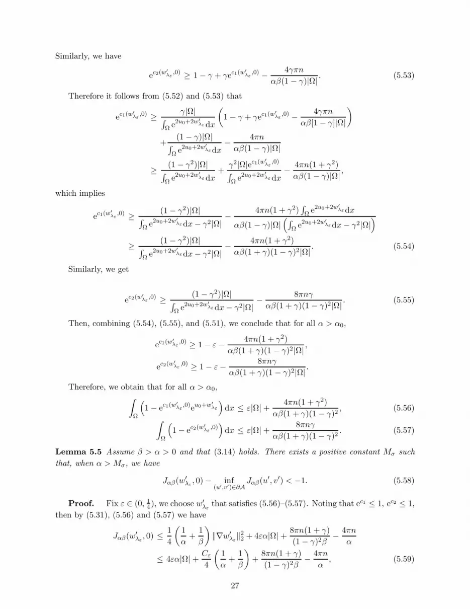
Similarly, we have
ec2(w′
λε,0) ≥ 1− γ + γec1(w
′
λε,0) − 4γπn
αβ(1− γ)|Ω| . (5.53)
Therefore it follows from (5.52) and (5.53) that
ec1(w′
λε,0) ≥ γ|Ω|
∫
Ω e2u0+2w′
λεdx
(
1− γ + γec1(w′
λε,0) − 4γπn
αβ[1 − γ]|Ω|
)
+(1− γ)|Ω|
∫
Ω e2u0+2w′
λεdx− 4πn
αβ(1− γ)|Ω|
≥ (1 − γ2)|Ω|∫
Ω e2u0+2w′
λεdx+γ2|Ω|ec1(w′
λε,0)
∫
Ω e2u0+2w′
λεdx− 4πn(1 + γ2)
αβ(1 − γ)|Ω| ,
which implies
ec1(w′
λε,0) ≥ (1− γ2)|Ω|
∫
Ω e2u0+2w′
λεdx− γ2|Ω|− 4πn(1 + γ2)
∫
Ω e2u0+2w′
λεdx
αβ(1 − γ)|Ω|(
∫
Ω e2u0+2w′
λεdx− γ2|Ω|)
≥ (1− γ2)|Ω|∫
Ω e2u0+2w′
λεdx− γ2|Ω|− 4πn(1 + γ2)
αβ(1 + γ)(1− γ)2|Ω| . (5.54)
Similarly, we get
ec2(w′
λε,0) ≥ (1− γ2)|Ω|
∫
Ω e2u0+2w′
λεdx− γ2|Ω|− 8πnγ
αβ(1 + γ)(1 − γ)2|Ω| . (5.55)
Then, combining (5.54), (5.55), and (5.51), we conclude that for all α > α0,
ec1(w′
λε,0) ≥ 1− ε− 4πn(1 + γ2)
αβ(1 + γ)(1 − γ)2|Ω| ,
ec2(w′
λε,0) ≥ 1− ε− 8πnγ
αβ(1 + γ)(1− γ)2|Ω| .
Therefore, we obtain that for all α > α0,∫
Ω
(
1− ec1(w′
λε,0)eu0+w
′
λε
)
dx ≤ ε|Ω|+ 4πn(1 + γ2)
αβ(1 + γ)(1− γ)2, (5.56)
∫
Ω
(
1− ec2(w′
λε,0))
dx ≤ ε|Ω|+ 8πnγ
αβ(1 + γ)(1− γ)2. (5.57)
Lemma 5.5 Assume β > α > 0 and that (3.14) holds. There exists a positive constant Mσ such
that, when α > Mσ, we have
Jαβ(w′λε, 0) − inf
(u′,v′)∈∂AJαβ(u
′, v′) < −1. (5.58)
Proof. Fix ε ∈ (0, 14), we choose w′λε
that satisfies (5.56)–(5.57). Noting that ec1 ≤ 1, ec2 ≤ 1,
then by (5.31), (5.56) and (5.57) we have
Jαβ(w′λε, 0) ≤ 1
4
(
1
α+
1
β
)
‖∇w′λε‖22 + 4εα|Ω| + 8πn(1 + γ)
(1− γ)2β− 4πn
α
≤ 4εα|Ω| + Cε
4
(
1
α+
1
β
)
+8πn(1 + γ)
(1− γ)2β− 4πn
α, (5.59)
27

where Cε is a positive constant depending only on ε.
Then by Lemma 5.4 we have
Jαβ(w′λε, 0) − inf
(u′,v′)∈∂AJαβ(u
′, v′)
≤ 2α|Ω|(2ε − 1) +Cε
4
(
1
α+
1
β
)
+8πn(1 + γ)
(1− γ)2β
+16πn
(1 + γ)(1− γ)2α+
4γ√
2πn|Ω|1− γ2
+ Cαβ , (5.60)
where Cαβ is defined by (5.41).
By the assumption β > α > 0 and (3.14), we easily deduce the following estimate
2
1 + σ≤ 1− γ < 1, (5.61)
Cαβ ≤ Cσ
(
lnα
α+ 1
)
(5.62)
with a suitable constant Cσ > 0 depending on σ > 1 only. By using the above estimates in (5.60),
we obtain the desired conclusion.
Using Lemma 5.3 and 5.5, we infer that under the assumption β > α > 0 and (3.14), when α
is sufficiently large the problem (5.30) admits a minimizer (u′α, v′α) , which lies in the interior of A.
Consequently,
DJαβ(u′α, v
′α) = 0,
and
uα = u′α + c1(u′α, v
′α), vα = v′α + c2(u
′α, v
′α) (5.63)
gives rise to a critical point for the functional Iαβ , namely, a weak solution to (5.6) and (5.7).
In what follows we study the behavior of the solution given by (5.63).
Lemma 5.6 Let (uα, vα) be defined by (5.63). Then
eu0+uα → 1, evα → 1 (5.64)
as α→ +∞ pointwise a.e. in Ω, and in Lp(Ω) for any p ≥ 1.
Proof. Using (5.59), we obtain that for any ε > 0 (small) there exists αε > 0 such that when
α > αε,
inf(u′,v′)∈A
Jαβ(u′, v′) ≤ 4εα|Ω| + Cε
4
(
1
α+
1
β
)
+8πn(1 + γ)
(1− γ)2β− 4πn
α. (5.65)
By a similar argument as in Lemma 5.3 we have
inf(u′,v′)∈A
Jαβ(u′, v′)
= Jαβ(u′α, v
′α)
≥ α
∫
Ω
(
eu0+uα + evα − 2)2
dx+ β
∫
Ω
(
eu0+uα − evα)2
dx− Cαβ
≥ 2α
(∫
Ω
[
eu0+uα − 1]2
dx+
∫
Ω[evα − 1]2 dx
)
−Cαβ , (5.66)
28

where Cαβ is defined by (5.41).
Then by means of (5.61), (5.62), (5.65), and (5.66), we see that
lim supα→+∞
(∫
Ω
[
eu0+uα − 1]2
dx+
∫
Ω[evα − 1]2 dx
)
≤ 2|Ω|ε, ∀ε > 0,
which enables us to conclude that,
eu0+uα → 1, evα → 1,
in L2(Ω), as α→ +∞. Since by Proposition 5.1, we also know that
eu0+uα < 1, evα < 1
in Ω. Then we have
eu0+uα → 1, evα → 1
pointwise a.e. in Ω as α → +∞. At this point, we may complete the proof of Lemma 5.6 by
dominated convergence theorem.
In order to get a secondary solution of (5.6) and (5.7), we first show that the solution (uα, vα)
given by (5.63) is a local minimizer of the functional Iαβ.
Lemma 5.7 Let (uα, vα) be defined by (5.63). Then (uα, vα) is a local minimizer of the functional
Iαβ in A.
Proof. It is easy to check that for any (u′, v′) ∈ A,
∂c1Iαβ(u′ + c1(u
′, v′), v′ + c2(u′, v′))
= 2(α+ β)
[
e2c1∫
Ωe2u0+2u′dx− ec1Q1(u
′, v′, ec2) +2πn
αβ
]
= 0,
∂c2Iαβ(u′ + c1(u
′, v′), v′ + c2(u′, v′))
= 2(α+ β)
[
e2c2∫
Ωe2u0+2u′dx− ec2Q2(u
′, v′, ec1) +2γπn
αβ
]
= 0,
and
∂2c21
Iαβ(u′ + c1(u
′, v′), v′ + c2(u′, v′))
= 2(α + β)
[
2e2c1∫
Ωe2u0+2u′dx− ec1Q1(u
′, v′, ec2)
]
,
∂2c22
Iαβ(u′ + c1(u
′, v′), v′ + c2(u′, v′))
= 2(α + β)
[
e2c2∫
Ωe2u0+2u′dx− ec2Q2(u
′, v′, ec1)
]
,
∂2c1c2Iαβ(u′ + c1(u
′, v′), v′ + c2(u′, v′))
= −2(α + β)γec1ec2∫
Ωeu0+u
′+v′dx.
29

Then, in view of (5.25) and (5.26), we obtain
∂2c21
Iαβ(uα, vα)
= 2(α+ β)
[
(1− γ)
∫
Ωeu0+uαdx+ γ
∫
Ωeu0+uα+vαdx
]2
− 8πn
αβ
∫
Ωe2u0+2uαdx
1
2
,
∂2c22
Iαβ(uα, vα)
= 2(α+ β)
[
(1− γ)
∫
Ωevαdx+ γ
∫
Ωeu0+uα+vαdx
]2
− 8γπn
αβ
∫
Ωe2vαdx
1
2
.
Since (u′α, v′α) lies in the interior of A, we obtain
∂2c21
Iαβ(uα, vα) > 2(α + β)γ
∫
Ωeu0+uα+vαdx,
∂2c22
Iαβ(uα, vα) > 2(α + β)γ
∫
Ωeu0+uα+vαdx.
Hence, at the point (uα, vα) the Hessian matrix of Iαβ(u′ + c1, v
′ + c2) with respect to (c1, c2) is
strictly positive definite. Let u = u′ + c1, v = v′ + c2. By continuity, there exists δ > 0 such that
for
‖u− uα‖+ ‖v − vα‖ ≤ δ,
we have (u′, v′) lies in the interior of A and
Iαβ(u, v) ≥ Iαβ(u′ + c1(u
′, v′), v′ + c2(u′, v′)) = Jαβ(u
′, v′).
Hence we have
Iαβ(u, v) ≥ Jαβ(u′, v′) ≥ inf
(u′,v′)∈AJαβ(u
′, v′) = Iαβ(uα, vα),
which says that (uα, vα) is a local minimizer of Iαβ(u, v).
5.2 The second solution
To find a secondary solution which is actually a mountain-pass critical point, we show that the
functional Iαβ satisfies the Palais–Smale condition.
Lemma 5.8 Let (um, vm) be a sequence in W 1,2(Ω)×W 1,2(Ω) satisfying
Iαβ(um, vm) → ν as m→ +∞, (5.67)
‖DIαβ(um, vm)‖∗ → 0 as m→ +∞, (5.68)
where ν is a constant, ‖ · ‖∗ denotes the norm of the dual space of W 1,2(Ω) × W 1,2(Ω). Then
(um, vm) admits a convergent subsequence in W 1,2(Ω)×W 1,2(Ω) .
Proof. Let um = c1,m + u′m, vm = c2,m + v′m, where
∫
Ωu′mdx = 0,
∫
Ωv′mdx = 0, c1,m =
1
|Ω|
∫
Ωumdx, c2,m =
1
|Ω|
∫
Ωvmdx.
30

A simple computation gives
(DIαβ(um, vm))(ϕ,ψ)
=1
2
(
1
α+
1
β
)∫
Ω(∇um · ∇ϕ+∇vm · ∇ψ)dx+
1
2
(
1
α− 1
β
)∫
Ω(∇vm · ∇ϕ+∇um · ∇ψ)dx
+2α
∫
Ω(eu0+um + evm − 2)eu0+umϕdx+ 2α
∫
Ω(eu0+um + evm − 2)evmψdx
+2β
∫
Ω(eu0+um − evm)eu0+umϕdx− 2β
∫
Ω(eu0+um − evm)evmψdx
+4πn
|Ω|
(
1
α+
1
β
)∫
Ωϕdx+
4πn
|Ω|
(
1
α− 1
β
)∫
Ωψdx. (5.69)
Taking (ϕ,ψ) = (1, 0) and (ϕ,ψ) = (0, 1) in (5.69), from (5.68) we obtain as m→ +∞,
(α+ β)
∫
Ωe2u0+2umdx− 2α
∫
Ωeu0+umdx− (β − α)
∫
Ωeu0+um+vmdx+ 2πn
(
1
α+
1
β
)
→ 0,(5.70)
(α+ β)
∫
Ωe2vmdx− 2α
∫
Ωevmdx− (β − α)
∫
Ωeu0+um+vmdx+ 2πn
(
1
α− 1
β
)
→ 0. (5.71)
Combining (5.70) and (5.71) gives
(α+ β)
∫
Ω
(
e2u0+2um + e2vm)
dx− 2(β − α)
∫
Ωeu0+um+vmdx
−2α
∫
Ω(eu0+um + evm)dx+
4πn
α→ 0 (5.72)
as m→ +∞.
Noting that
α(
eu0+um + evm − 2)2
+ β(
eu0+um − evm)2
= (α+ β)(
e2u0+2um + e2vm)
− 2(β − α)eu0+um+vm − 4α(eu0+um + evm) + 4α
and
α(
eu0+um + evm − 2)2
+ β(
eu0+um − evm)2 ≥ α
(
[
eu0+um + evm − 2]2
+[
eu0+um − evm]2)
= 2α(
[
eu0+um − 1]2
+ [evm − 1]2)
,
by (5.72) we have
2α
∫
Ω
[
(
eu0+um − 1)2
+ (evm − 1)2]
dx+ 2α
∫
Ω
(
eu0+um + evm)
dx+4πn
α< 4|Ω|α + o(1)(5.73)
as m→ +∞.
Then it follows from (5.73) that
∫
Ω
(
eu0+um + evm − 2)2
dx+
∫
Ω
(
eu0+um − evm)2
dx ≤ 4|Ω|+ o(1), (5.74)
∫
Ω
(
eu0+um − 1)2
dx+
∫
Ω(evm − 1)2 dx ≤ 2|Ω|+ o(1), (5.75)
∫
Ωeu0+umdx ≤ 2|Ω|+ o(1),
∫
Ωevmdx ≤ 2|Ω|+ o(1), (5.76)
31

as m→ +∞.
Using (5.76) and the Jensen inequality we obtain
ec1,m ≤ 2 + o(1), ec2,m ≤ 2 + o(1), (5.77)
as m→ +∞, which says c1,m, c2,m are bounded from above. From (5.75)–(5.76) we see that∫
Ωe2u0+2umdx ≤ 6|Ω|+ o(1),
∫
Ωe2vmdx ≤ 6|Ω|+ o(1), (5.78)
as m→ +∞.
Denote (u′m + v′m)+ ≡ maxu′m + v′m, 0. Setting ϕ = ψ = (u′m + v′m)
+ in (5.69), we have
(DIαβ(um, vm))[
(u′m + v′m)+, (u′m + v′m)
+]
=1
α‖∇(u′m + v′m)
+‖22 + 2(α + β)
∫
Ω
(
eu0+um − evm)2
(u′m + v′m)+dx
+8α
∫
Ωeu0+um+vm(u′m + v′m)
+dx− 4α
∫
Ω
(
eu0+um + evm)
(u′m + v′m)+dx
+8πn
α|Ω|
∫
Ω(u′m + v′m)
+dx
≥ 8α
∫
Ωeu0+um+vm(u′m + v′m)
+dx− 4α
∫
Ω
(
eu0+um + evm)
(u′m + v′m)+dx
≥ 8α
∫
Ωeu0+um+vm(u′m + v′m)
+dx
−4α
(
[∫
Ωe2u0+2umdx
]1
2
+
[∫
Ωe2vmdx
]1
2
)
‖(u′m + v′m)+‖2. (5.79)
Then it follows from (5.68), (5.78) and (5.79) that∫
Ωeu0+um+vm(u′m + v′m)
+dx ≤ C(
‖(u′m + v′m)+‖2 + εn‖(u′m + v′m)
+‖)
≤ C(
‖∇u′m‖2 + ‖∇v′m‖2)
, (5.80)
where C is a suitable positive constant independent of m and εm → 0 as m→ ∞.
Now let (ϕ,ψ) = (u′m, v′m) in (5.69), we see that
(DIαβ(um, vm))(u′m, v
′m)
≥ 1
β
(
‖∇u′m‖22 + ‖∇v′m‖22)
+ 2(α+ β)
∫
Ωe2u0+2umu′mdx
−4α
∫
Ωeu0+umu′mdx+ 2(α+ β)
∫
Ωe2vmv′mdx− 4α
∫
Ωevmv′mdx
−2(β − α)
∫
Ωeu0+um+vm(u′m + v′m)
+dx
≥ 1
β
(
‖∇u′m‖22 + ‖∇v′m‖22)
+ 2(α+ β)
[∫
Ωe2u0e2c1,m(e2u
′
m − 1)u′mdx+∫
Ωe2u0e2c1,mu′mdx
]
+2(α + β)
[∫
Ωe2c2,m(e2v
′
m − 1)v′mdx+
∫
Ωe2c2,mv′mdx
]
−4α
[
(∫
Ωe2u0+2umdx
)1
2
‖∇u′m‖2 +(∫
Ωe2vmdx
)1
2
‖∇v′m‖2]
− C(
‖∇u′m‖2 + ‖∇v′m‖2)
≥ 1
β
(
‖∇u′m‖22 + ‖∇v′m‖22)
− C(
‖∇u′m‖2 + ‖∇v′m‖2)
, (5.81)
32

where we have used (5.77)–(5.80) and the Holder inequality, C is a positive constant independent
of m.
Then using (5.68)–(5.81), we conclude that there exits a positive constant C independent of m
such that
‖∇u′m‖2 + ‖∇v′m‖2 ≤ C. (5.82)
On the other hand, from (5.67) we see that Iαβ(um, vm) is bounded from below. Therefore we
have
4πn
[(
1
α+
1
β
)
c1,m +
(
1
α− 1
β
)
c2,m
]
≥ −C − α
∫
Ω
(
eu0+um + evm − 2)2
dx− β
∫
Ω
(
eu0+um − evm)2
dx
− 1
2α
(
‖∇u′m‖22 + ‖∇v′m‖22)
≥ −C, (5.83)
where we have used (5.74) and (5.82), C is a positive constant independent of m. Then we infer
from (5.77) and (5.83) that c1,m, c2,m are bounded from below uniformly with respect to m. As a
result c1,m, c2,m are bounded for all m. Therefore we obtain that um = u′m + c1,m, vm = v′m + c2,m
are bounded sequence in W 1,2(Ω). Hence there exists a subsequence of um and vm, still denoted
by um and vm, such that
um → u, vm → v
weakly in W 1,2(Ω), strongly in Lp(Ω) for any p ≥ 1 and pointwise a.e. in Ω as m → ∞, where
u, v ∈W 1,2(Ω). Moreover, we see that
eum → eu, evm → ev strongly in Lp(Ω), ∀ p ≥ 1
and
c1,m =1
|Ω|
∫
Ωumdx→ c1 =
1
|Ω|
∫
Ωudx, c2,m =
1
|Ω|
∫
Ωvmdx→ c2 =
1
|Ω|
∫
Ωvdx
as m→ ∞.
Hence, for any (ϕ,ψ) ∈W 1,2(Ω)×W 1,2(Ω), as m→ ∞ we have
I ′αβ(um, vm)(ϕ,ψ) → I ′αβ(u, v)(ϕ,ψ) = 0, (5.84)
which says that (u, v) is a critical point for the functional Iαβ .
In the sequel we show the strong convergence of (um, vm). Let (ϕ,ψ) = (um− u, vm− v). Then,from (5.68) and (5.84), we see that
[DIαβ(um, vm)−DIαβ(u, v)][um − u, vm − v] ≤ εn (‖um − u‖+ ‖vm − v‖) = o(1), (5.85)
as m→ ∞.
33

Then from (5.85) we conclude that
1
β
(
‖∇(um − u)‖22 + ‖∇(vm − v)‖22)
≤ −2(α+ β)
(∫
Ωe2u0 [e2um − e2u][um − u]dx+
∫
Ω[e2vm − e2v][vm − v]dx
)
+2(α− β)
∫
Ωeu0(eum+vm − eu+v)([um − u] + [vm − v])dx
+4α
∫
Ω
(
eu0 [eum − eu][um − u] + [evm − ev ][vm − v])
dx+ o(1)
= o(1),
as m → ∞. Therefore we see that (um, vm) converges strongly to (u, v) in W 1,2(Ω) ×W 1,2(Ω) as
m→ ∞. Then the lemma follows.
We have shown that, for α large enough, there exists a solution (uα, vα) of (5.6)–(5.7) satisfying
the behavior
eu0+uα → 1, evα → 1,
as α → +∞ and this solution is a local minimum for Iαβ by Lemma 5.7. Then there exists a
positive constant δ0 > 0 such that
Iαβ(u, v) ≥ Iαβ(uα, vα) if ‖u− uα‖+ ‖v − vα‖ ≤ δ0.
To find a secondary solution, we note that the functional admits a mountain-pass structure.
Indeed, noting that u0 + uα < 0, vα < 0, we have for all c < 0,
Iαβ(uα + c, vα)− Iαβ(uα, vα) ≤ (4α + β)|Ω|+ 4πn
(
1
α+
1
β
)
c. (5.86)
We consider two situations.
(1) If (uα, vα) is not a strictly local minimum for the functional Iαβ, i.e., for all 0 < δ < δ0,
inf‖u−uα‖+‖v−vα‖=δ
Iαβ(u, v) = Iαβ(uα, vα).
Then by using Ekeland’s lemma (see [25]), we get a local minimum (uδα, vδα) for Iαβ such that
‖uδα − uα‖+ ‖vδα − vα‖ = δ for any δ ∈ (0, δ0).
Of course, we can find a secondary solution.
(2) If (uα, vα) is a strictly local minimum for the functional Iαβ, then there exits δ1 ∈ (0, δ0)
such that
inf‖u−uα‖+‖v−vα‖=δ1
Iαβ(u, v) > Iαβ(uα, vα).
Moreover, in view of (5.86) we can choose |c| > δ0 such that
Iαβ(uα + c, vα) < Iαβ(uα, vα)− 1
Now we introduce the paths
P =
Γ(t)|Γ ∈ C(
[0, 1];W 1,2(Ω)×W 1,2(Ω))
: Γ(0) = (uα, vα), Γ(1) = (uα + c, vα)
34

and define
m0 = infΓ∈P
supt∈[0,1]
Iαβ(Γ(t))
.
Hence we have
m0 > Iαβ(uα, vα). (5.87)
Then by Lemma 5.8 we see that the functional Iαβ satisfies all the hypotheses of the mountain-pass
theorem of Ambrosetti–Rabinowitz [3]. Therefore we conclude that m0 is a critical value of the
functional Iαβ. Noting (5.87), we have an additional solution of the equations (5.6) and (5.7).
Then the proof of Theorem 3.2 is complete.
6 Summary and comments
In this paper, we developed an existence theory for the multiple vortex solutions of the non-
Abelian Chern–Simons–Higgs equations in the Gudnason model [27,28] of N = 2 supersymmetric
field theory where gauge field dynamics is governed by two Chern–Simons terms. In the full-
plane situation, we proved the existence of solutions for the general system of nonlinear partial
differential equations involving an arbitrary number of unknowns and established the exponential
decay estimates for the solutions which realize a family of quantized integrals expressed in terms
of vortex numbers. These solutions give rise to multiple vortex field configurations which approach
at spatial infinity the vacuum state with completely broken symmetry and known as topological
solutions. There are no restrictions to the values of various coupling parameters and vortex numbers
or vortex distributions for the existence results to hold. In the doubly periodic domain setting,
we confined our study to the case when the vortex equations contain only two unknowns. We
derived a necessary condition for the existence of a multiple vortex solution and obtained some
sufficient conditions for the existence of two distinct solutions for a given prescribed distribution
of vortices. We also established the asymptotic behavior of the solutions as a coupling parameter
goes to infinity.The problems which remain untouched and are of considerable future interest are the existence
of nontopological solutions realizing the asymptotic vacuum state with unbroken symmetry andthe existence of solutions of the multiple vortex equations involving more than two unknowns. Ourmethods developed so far are still not sufficiently effective in dealing with these rather challengingproblems and new ideas and techniques are called upon in order to make further progress in thisarea.
References
[1] A. A. Abrikosov, On the magnetic properties of superconductors of the second group, Sov. Phys. JETP
5 (1957) 1174–1182.
[2] O. Aharony, O. Bergman, D. L. Jaferis and J. Maldacena, N = 6 superconformal Chern-Simons-matter
theories, M2-branes and their gravity duals, J. High Energy Phys. 0810 (2008) 091.
[3] A. Ambrosetti and P. Rabinowitz, Dual variational methods in critical point theory and applications,
J. Funct. Anal. 14 (1973) 349–381.
[4] T. Aubin, Nonlinear Analysis on Manifolds: Monge–Ampere Equations, Springer, Berlin and New York,
1982.
35

[5] R. Auzzi, S. Bolognesi, J. Evslin, K. Konishi, and A. Yung, Nonabelian superconductors: vortices and
confinement in N = 2 SQCD, Nucl. Phys. B 673 (2003) 187–216.
[6] J. Bagger and N. Lambert, Modeling multiple M2’s, Phys. Rev. D 75 (2007) 045020.
[7] J. Bagger and N. Lambert, Gauge symmetry and supersymmetry of multiple M2-branes, Phys. Rev. D
77 (2008) 065008.
[8] J. Bagger and N. Lambert, Comments on multiple M2-branes, J. High Energy Phys. 0802 (2008) 105.
[9] A. Bezryadina, E. Eugenieva, and Z. Chen, Self-trapping and flipping of double-charged vortices in
optically induced photonic lattices, Optics Lett. 31 (2006) 2456–2458.
[10] E. B. Bogomol’nyi, The stability of classical solitons, Sov. J. Nucl. Phys. 24 (1976) 449–454.
[11] L. Caffarelli and Y. Yang, Vortex condensation in the Chern–Simons Higgs model: an existence theorem,
Commun. Math. Phys. 168 (1995) 321–336.
[12] D. Chae and O. Yu. Imanuvilov, The existence of nontopological multivortex solutions in the relativistic
self-dual Chern–Simons theory, Commun. Math. Phys. 215, 119–142 (2000).
[13] M. Chaichian and N. F. Nelipa, Introduction to Gauge Field Theory, Springer, Berlin and New York,
1984.
[14] H. Chan, C.-C. Fu, and C.-S. Lin, Non-topological multi-vortex solutions to the self-dual Chern–Simons–
Higgs equations, Commun. Math. Phys. 231 (2002) 189–221.
[15] R. M. Chen, Y. Guo, D. Spirn, and Y. Yang, Electrically and magnetically charged vortices in the
Chern–Simons–Higgs theory, Proc. Roy. Soc. A 465 (2009) 3489–3516.
[16] X. Chen, S. Hastings, J. B. McLeod, and Y. Yang, A nonlinear elliptic equation arising from gauge field
theory and cosmology, Proc. Roy. Soc. A 446, 453–478 (1994).
[17] S. S. Chern and J. Simons, Some cohomology classes in principal fiber bundles and their application to
Riemannian geometry, Proc. Nat. Acad. Sci. USA 68 (1971) 791–794.
[18] S. S. Chern and J. Simons, Characteristic forms and geometric invariants, Ann. Math. 99 (1974) 48–69.
[19] S. Deser, R. Jackiw, and S. Templeton, Three-dimensional massive gauge theories, Phys. Rev. Lett. 48
(1982) 975–978.
[20] S. Deser, R. Jackiw, and S. Templeton, Topologically massive gauge theories, Ann. Phys. 140 (1982)
372–411.
[21] Q. Du, M. Gunzburger, and J. Peterson, Analysis and approximation of the Ginzburg–Landau model
of superconductivity, SIAM Rev. 34 (1992) 54–81.
[22] G. Dunne, Self-Dual Chern–Simons Theories, Lecture Notes in Physics, vol. m 36, Springer, Berlin,
1995.
[23] G. Dunne, R. Jackiw, S.-Y. Pi, and C. Trugenberger, Self-dual Chern–Simons solitons and two-
dimensional nonlinear equations, Phys. Rev. D 43 (1991) 1332–1345.
[24] L. Fontana, Sharp borderline Sobolev inequalities on compact Riemannian manifolds, Comment. Math.
Helv. 68 (1993) 415–454.
[25] N. Ghoussoub, Duality and Perturbation Methods in Critical Point Theory, Cambridge University Press,
Cambridge, U. K., 1993.
[26] V. L. Ginzburg and L. D. Landau, On the theory of superconductivity, in Collected Papers of L. D.
Landau (edited by D. Ter Haar), pp. 546–568, Pergamon, New York, 1965.
36

[27] S. B. Gudnason, Non-abelian Chern–Simons vortices with generic gauge groups, Nucl. Phys. B 821
(2009) 151–169.
[28] S. B. Gudnason, Fractional and semi-local non-Abelian Chern–Simons vortices, Nucl. Physics B 840
(2010) 160–185.
[29] A. Gustavsson, Algebraic structures on parallel M2-branes, Nucl. Phys. B 811 (2009) 66–76.
[30] X. Han and G. Tarantello, Doubly periodic self-dual vortices in a relativistic non-Abelian Chern–Simons
model, Calc. Var. and PDE, DOI 10.1007/s00526-013-0615-7.
[31] A. Hanany, M. J. Strassler, and A. Zaffaroni, Confinement and strings in MQCD, Nucl. Phys. B 513
(1998) 87–118.
[32] A. Hanany and D. Tong, Vortices, instantons and branes, J. High Energy Phys. 0307 (2003) 037.
[33] J. Hong, Y. Kim and P.-Y. Pac, Multivortex solutions of the Abelian Chern–Simons–Higgs theory, Phys.
Rev. Lett. 64 (1990) 2330–2333.
[34] P. A. Horvathy and P. Zhang, Vortices in (Abelian) Chern–Simons gauge theory, Phys. Rep. 481 (2009)
83–142.
[35] K. Huang, Quarks, Leptons, and Gauge Fields, 2nd ed., World Scientific, Singapore, 1992.
[36] S. Inouye, S. Gupta, T. Rosenband, A. P. Chikkatur, A. Gorlitz, T. L. Gustavson, A. E. Leanhardt, D.
E. Pritchard and W. Ketterle, Observation of vortex phase singularities in Bose-Einstein condensates,
Phys. Rev. Lett. 87 (2001), 080402.
[37] R. Jackiw, S.-Y. Pi, and E. J. Weinberg, Topological and non-topological solitons in relativistic and
non-relativistic Chern–Simons theory, Particles, Strings and Cosmology (Boston, 1990), pp. 573–588,
World Sci. Pub., River Edge, NJ, 1991.
[38] R. Jackiw and S. Templeton, How super-renormalizable interactions cure their infrared divergences,
Phys. Rev. D 23 (1981) 2291–2304.
[39] R. Jackiw and E. J. Weinberg, Self-dual Chern–Simons vortices, Phys. Rev. Lett. 64 (1990) 2334–2337.
[40] A. Jaffe and C. H. Taubes, Vortices and Monopoles, Birkhauser, Boston, 1980.
[41] B. Julia and A. Zee, Poles with both magnetic and electric charges in non-Abelian gauge theory, Phys.
Rev. D 11 (1975) 2227–2232.
[42] Y. Kawaguchi and T. Ohmi, Splitting instability of a multiply charged vortex in a Bose–Einstein
condensate, Phys. Rev. A 70 (2004) 043610.
[43] D. I. Khomskii and A. Freimuth, Charged vortices in high temperature superconductors, Phys. Rev.
Lett. 75 (1995) 1384–1386.
[44] C. N. Kumar and A. Khare, Charged vortex of finite energy in nonabelian gauge theories with Chern–
Simons term, Phys. Lett. B 178 (1986) 395–399.
[45] C.-S. Lin, J. Wei, and D. Ye, Classification and nondegeneracy of SU(n+1) Toda system with singular
sources, Invent. Math. 190 (2012) 169–207.
[46] A. Marshakov and A. Yung, Non-Abelian confinement via Abelian flux tubes in softly broken N = 2
SUSY QCD, Nucl. Phys. B 647 (2002) 3–48.
[47] Y. Matsuda, K. Nozakib, and K. Kumagaib, Charged vortices in high temperature superconductors
probed by nuclear magnetic resonance, J. Phys. Chem. Solids 63 (2002) 1061–1063.
[48] M. Nolasco and G. Tarantello, Vortex condensates for the SU(3) Chern–Simons theory, Commun. Math.
Phys. 213 (2000) 599–639.
37

[49] M. Nolasco and G. Tarantello, On a Sharp Sobolev-tupe Inequality on Two-Dimensional Compact
Manifolds, Arch. Rational Mech. Anal. 145 (1998) 161–195.
[50] M. Nolasco and G. Tarantello, Double vortex condensates in the Chern-Simons-Higgs theory, Calc. Var.
and PDE 9 (1999), 31–94.
[51] S. Paul and A. Khare, Charged vortices in an Abelian Higgs model with Chern–Simons term, Phys.
Lett. B 17 (1986) 420–422.
[52] M. K. Prasad and C. M. Sommerfield, Exact classical solutions for the ’t Hooft monopole and the
Julia–Zee dyon, Phys. Rev. Lett. 35 (1975) 760–762.
[53] L. H. Ryder, Quantum Field Theory, 2nd edition, Cambridge U. Press, London, 1996.
[54] J. S. Schonfeld, A massive term for three-dimensional gauge fields, Nucl. Phys. B 185 (1981) 157–171.
[55] N. Seiberg and E. Witten, Monopole condensation, and confinement in N=2 supersymmetric Yang-Mills
theory, Nucl. Phys. B 426 (1994) 19–52. Erratum – ibid. B 430 (1994) 485–486.
[56] S. I. Shevchenko, Charged vortices in superfluid systems with pairing of spatially separated carriers,
Phys. Rev. B 67 (2003) 214515.
[57] M. Shifman, and A. Yung, Supersymmetric solitons and how they help us understand non-Abelian
gauge theories Rev. Mod. Phys. 79 (2007) 1139.
[58] M. Shifman and A. Yung, Supersymmetric Solitons, Cambridge U. Press, Cambridge, U. K., 2009.
[59] J. B. Sokoloff, Charged vortex excitations in quantum Hall systems, Phys. Rev. B 31 (1985) 1924–1928.
[60] J. Spruck and Y. Yang, Topological solutions in the self-dual Chern–Simons theory: existence and
approximation, Ann. Inst. H. Poincare – Anal. non lineaire, 12, (1995) 75–97 .
[61] J. Spruck and Y. Yang, The existence of non-topological solitons in the self-dual Chern–Simons theory,
Commun. Math. Phys. 149, 361–376 (1992).
[62] J. Spruck and Y. Yang, Proof of the Julia–Zee theorem, Commun. Math. Phys. 291 (2009) 347–356.
[63] G. Tarantello, Multiple condensate solutions for the Chern–Simons–Higgs theory, J. Math. Phys. 37
(1996) 3769–3796.
[64] G. Tarantello, Self-Dual Gauge Field Vortices, an Analytic Approach, Progress in Nonlinear Differential
Equations and Their Applications 72, Birkhauser, Boston, Basel, Berlin, 2008.
[65] C. H. Taubes, Arbitrary N -vortex solutions to the first order Ginzburg–Landau equations, Commun.
Math. Phys. 72 (1980) 277–292.
[66] H.J. de Vega and F. Schaposnik, Electrically charged vortices in non-Abelian gauge theories with Chern–
Simons term, Phys. Rev. Lett. 56 (1986) 2564–2566.
[67] H.J. de Vega and F. Schaposnik, Vortices and electrically charged vortices in non-Abelian gauge theories,
Phys. Rev. D, 34 (1986) 3206–3213.
[68] A. Vilenkin and E. P. S. Shellard, Cosmic Strings and Other Topological Defects, Cambridge U. Press,
Cambridge, 1994.
[69] R. Wang, The existence of Chern–Simons vortices, Commun. Math. Phys. 137 (1991) 587–597.
[70] S. Wang and Y. Yang, Abrikosov’s vortices in the critical coupling, SIAM J. Math. Anal. 23 (1992)
1125–1140.
[71] Y. Yang, Obstructions to the existence of static cosmic strings in an Abelian Higgs model, Phys. Rev.
Lett. 73, 10–13 (1994).
38

[72] Y. Yang, Prescribing topological defects for the coupled Einstein and Abelian Higgs equations, Commun.
Math. Phys. 170, 541–582 (1995).
[73] Y. Yang, The relativistic non-Abelian Chern–Simons equations, Commun. Math. Phys. 186 (1997)
199–218.
[74] Y. Yang, Solitons in Field Theory and Nonlinear Analysis, Springer-Verlag, New York, 2001.
39