arX

iv:h

ep-t

h/91

1006

9v1

29

Oct

199

1

US-FT-10/91

October, 1991

ANALYSIS OF OBSERVABLES IN

CHERN-SIMONS PERTURBATION THEORY

M. Alvarez and J.M.F. Labastida⋆

Departamento de Fısica de Partıculas

Universidade de Santiago

E-15706 Santiago de Compostela, Spain

ABSTRACT

Chern-Simons Theory with gauge group SU(N) is analyzed from a perturba-

tion theory point of view. The vacuum expectation value of the unknot is computed

up to order g6 and it is shown that agreement with the exact result by Witten im-

plies no quantum correction at two loops for the two-point function. In addition, it

is shown from a perturbation theory point of view that the framing dependence of

the vacuum expectation value of an arbitrary knot factorizes in the form predicted

by Witten.

⋆ E-mail: LABASTIDA@EUSCVX.DECNET

1. Introduction

Chern-Simons gauge theory was solved exactly by Witten [1] using non-

perturbative methods. This solution has been obtained subsequently by other

groups using both, the point of view of canonical quantization [2-10], and of cur-

rent algebra [11,5] as originally proposed in [1]. The exact result for the vacuum

expectation value of the observables of the theory is analytic in the inverse of

the Chern-Simons parameter k. Defining the Chern-Simons coupling constant as

g =√

4π/k the exact result suggests that the small coupling constant pertur-

bation expansion should reproduce the exact result. One does not expect any

non-perturbative effect in Chern-Simons gauge theory. Perturbative approaches

to the theory under consideration have been carried out during the last two years

[12-25]. The main question which have been addressed in these works is which one

is the renormalization scheme which leads to the exact result obtained by Witten.

In Chern-Simons gauge theory there are two problems which must be taken into

account. On the one hand, the loop expansion possesses divergences already at one

loop for two-point functions which must be regularized. On the other hand, some

of the observables of the theory, the Wilson lines, possess products of operators at

coincident points in their integration regions. The loop expansion divergences must

be regulated in perturbation theory to obtain a finite answer to be compared to

the exact result. The ambiguities present when considering products of operators

at coincident points forces to make a choice in defining the observables of the the-

ory. The main goal of this paper is to give a regularization procedure and a choice

to solve the problem of the ambiguity when considering products of operators at

coincident points whose perturbative expansion coincides with the exact result [1].

The second aspect of the problem was solved successfully in [12] and we will follow

here their approach.

To handle the ambiguity associated to products of operators at coincident

points one must consider framed links instead of links [26,1,12], in other words one

must introduce a band instead of a knot and the corresponding integer number

1

n which indicates the number of times that the band is twisted. In the non-

perturbative approach leading to the exact result [1] the origin of the dependence

on the framing comes about because one must construct the observables on the

surface of a Riemann surface which then must be glued to another Riemann surface

to build a three-dimensional manifold. The same knot can be obtained using that

procedure in a variety of ways leading to different quantities for observables which,

however, differ by a factor which is associated to the framing. As first found

out in [1] this factor is just exp(2πinh) where h is the conformal weight of the

representation (for SU(N) in the fundamental representation, h =c2(R)/(k + N),

c2(R) = (N2 − 1)/2N) carried out by the Wilson line.

The presence of ultraviolet divergences in the loop expansion of Chern-Simons

theory forces to regularize the theory and consequently to choose a renormaliza-

tion scheme. Certainly, from a perturbation theory point of view all schemes are

physically equivalent since they differ by a finite renormalization which can be ac-

complished by adding finite counterterms to the action. However, one would like

to know if there exist a scheme which leads naturally to the exact result obtained

by Witten. By naturalness we understand a scheme in which the intermediate

regularized action leads after taking the limit in which the cutoff is removed to

the exact result obtained by Witten where the constant k we started with (bare

k) is the same constant k as the one appearing in the exact result. Certainly, this

concept of naturalness has only meaning in a theory like Chern-Simons theory in

which the beta function as well as the anomalous dimensions of the elementary

fields vanish at any order in perturbation theory [20,21,24,27]. This was the point

of view taken in [13] where a scheme based on Pauli-Villars regularization seemed

to be natural in the sense discussed above. Indeed, the results obtained in [13]

showed that a choice of scheme of that type seems to lead to the shift k→k + N

which appears in many of the equations corresponding to the exact result. The

fact that the origin of the shift is a quantum effect was first pointed out by Witten

[1] who showed its appearance using a gauge invariant regularization based on the

eta function. There are other schemes which lead to results in agreement with

2

[13,1] as the one used in [18]. All these schemes which seem to provide at one

loop an explanation of the origin of the shift share the common feature that the

intermediate regularized action is gauge invariant.

So far all calculations involving quantum corrections using gauge invariant

regularized actions have concentrated on the effective action. The fact that the

quantum correction leads to an effective action whose constant k has been shifted

indicates that one would observe such effect when computing observables using

those schemes. However, at present, only indirect calculations of observables have

been carried out taking into account this quantum correction [25,12]. In this paper

we are going to present the computation of the Wilson line corresponding to the

unknot in the fundamental representation of SU(N) up to order g6. This calcu-

lation involves diagrams at two-loops for the two-point function whose calculation

in some scheme whose regularized action is gauge invariant has to be carried out.

We do not perform in this paper such a two-loop calculation but we will show that

agreement with the exact result implies that there is no correction a two-loops for

the two-point function. The computation of the two-point function at two-loops

using the Pauli-Villars regularization plus higher derivatives proposed in [13] is

being carried out [28]. So far we have been able to prove that there is no need to

introduce higher derivative terms to regulate the theory at two loops and that a

single generation of Pauli-Villars is sufficient to render the two-loop graphs finite.

However, we have not finished the calculation of the finite part that according

to the results which we present in this work should be zero to have agreement

with the exact result, and, therefore, to be able to consider the scheme based on

Pauli-Villars as natural.

To end with this introduction we will reproduce here the result obtained by

Witten in [1] for the framed unknot in the fundamental representation of SU(N)

lying on S3 with framing n. The corresponding vacuum expectation value is,

〈W 〉 =q

N

2 − q−N

2

q12 − q−

12

qnN2−1

2N , (1.1)

3

where,

q = exp(2πi

k + N). (1.2)

Expanding (1.1) in terms of 1/k up to terms of order 1/k3 one finds,

〈W 〉 = N +1

kiπn(N2 − 1)

+1

k2

[

−π2

6N(N2 − 1) −

π2n2

2N(N2 − 1)2 − iπnN(N2 − 1)

]

+1

k3

[

−iπ3

6n(N2 − 1)2 −

iπ3

6N2n3(N2 − 1)3 + π2n2(N2 − 1)2

+π2

3N2(N2 − 1) + iπnN2(N2 − 1)

]

+ O(1

k4).

(1.3)

Notice that in this expansion all terms containing a power of π different that the

power of 1/k are originated by the fact that k appears shifted into k + N in (1.2).

In our analysis we will show that those terms do indeed correspond to diagrams

which contain one-loop quantum corrections. Notice also that in the standard

framing (n = 0) the series expansion has a simpler form. As a consequence of

our analysis we will be able to identify very simply all diagrams which provide the

framing dependence. Actually, we will derive from a perturbation theory point of

view the form of the framing dependence of the vacuum expectation value of an

arbitrary knot. If, on the other hand, it turns to be correct the picture in which

there are only one-loop corrections (which just account for the shift k→k +N) one

could extract all the effects due to framing and therefore one would be left with

a series of diagrams which constitute the building blocks of the knot invariant.

These building blocks lead to topological invariants which after considering them

as the coefficients of a power series build the knot invariants leading to the Jones

polynomials [29] and its cousins [30,31]. We will discuss in more detail this picture

of the perturbation theory series expansion in our concluding remarks.

In this paper we will consider the three dimensional manifold as R3 which allows

us to identify the corresponding observables to the ones in S3. We will not discuss

4

the effect of the framing of the three-dimensional manifold from a perturbation

theory point of view. A good discussion of this point can be found in [25].

The paper is organized as follows. In sect. 2 we define the regularized Chern-

Simons gauge theory using Pauli-Villars fields which we claim to correspond to

a natural scheme in the sense discussed above. In sect. 3 we compute (1.3) in

perturbation theory the vacuum expectation value of the unknot carrying the fun-

damental representation of SU(N) up to order g6. In sect. 4 we will identify all

the framing dependence of the vacuum expectation value of a knot and we will

show its factorization in the form predicted by Witten. Finally, in sect. 5 we state

our conclusions and make some final remarks . Several appendices deal with our

conventions and with the proof of some results which are used in sects. 3 and 4.

5

2. Perturbative Chern-Simons gauge theory

In this section we will define Chern-Simons gauge theory from a perturbation

theory point of view. This is carried out in two steps. First a gauge fixing is

performed. Second, after analyzing the ultraviolet behavior of the theory a reg-

ularized action using Pauli-Villars fields is provided. Let us consider an SU(N)

gauge connection Aµ on a boundaryless three-dimensional manifold M and the

following Chern-Simons action,

S(Aµ) =k

4π

∫

M

Tr(A ∧ dA +2

3A ∧ A ∧ A), (2.1)

where k is an arbitrary positive integer⋆

and “Tr” denotes the trace in the fun-

damental representation of SU(N) (normalized in such a way that Tr(T aT b) =

−12δab). A summary of our group-theoretical conventions is contained in Appendix

A. In defining the theory from a perturbation theory point of view we must give a

meaning to vacuum expectation values of operators, i.e., to quantities of the form,

〈O〉 =1

Z

∫

[DAµ]O exp(

iS(Aµ))

, (2.2)

where Z is the partition function,

Z =

∫

[DAµ] exp(

iS(Aµ))

. (2.3)

The operators entering (2.2) are gauge invariant operators which do not depend on

the three-dimensional metric. These operators are knots, links and graphs [1,32].

The first issue in defining (2.2) is to take care of the gauge fixing. Indeed, the

⋆ A negative k will change the ǫ prescription in the perturbative series expansion leading toa shift of k at one loop with the opposite sign. With a negative k one makes connectionwith the exact result (1.1) after replacing q→q∗.

6

exponential in (2.2) is invariant under gauge transformations of the form,

Aµ→h−1Aµh + h−1∂µh, (2.4)

where h is an arbitrary continuous map h : M→SU(N). Before carrying out the

gauge fixing let us redefine the constant k and the field Aµ in such a way that

the action (2.1) becomes standard from a perturbation theory point of view. We

define,

g =

√

4π

k. (2.5)

Then, after rescaling the gauge connection,

Aµ→gAµ, (2.6)

one obtains the following Chern-Simons action,

S′(Aµ) =

∫

M

Tr(A ∧ dA +2

3gA ∧ A ∧ A). (2.7)

This form of the action contains the standard 1/2 factor for the kinetic term

after using (A3). From now on we will restrict ourselves to the case in which

the three-dimensional manifold M is R3 which is the simplest case to treat from a

perturbation theory point of view. Though (2.7) is metric independent, we will be

forced to introduce a metric in carrying out the gauge fixing. We will assume that

this metric has signature (1,−1,−1).

Our gauge choice will be the same as the one taken in [13]. The Lorentz-like

gauge condition ∂µAµ = 0 is imposed using the standard Fadeev-Popov construc-

tion which leads to the following action to be added to (2.7),

Sgf(Aµ, c, c, φ) =

∫

Tr(

2c∂µDµc − 2φ∂µAµ − λφ2)

, (2.8)

where φ is the Lagrange multiplier which imposes the gauge condition, c and c

are the Fadeev-Popov ghost, and λ is a gauge fixing parameter. In (2.8), Dµ is

7

the covariant derivative, Dµc = ∂µc + g[Aµ, c]. The action (2.7) as well as the

gauge-fixing action (2.8) are invariant under the following BRST transformations,

sAµ = Dµc, sc = −cc, sc = φ, sφ = 0. (2.9)

The field φ can be integrated out easily providing the following functional integral

for vacuum expectation values as the ones in (2.2):

〈O〉 =1

Z

∫

[DAµDcDc]O exp(

iI(Aµ, c, c))

, (2.10)

where,

I(Aµ, c, c) =

∫

Tr(

ǫµνρ(Aµ∂νAρ +2

3AµAνAρ) − λ−1Aµ∂µ∂νAν + 2c∂µDµc

)

.

(2.11)

Of course, Z in (2.10) is appropriately defined taking into account the gauge fixing.

The quantities obtained in (2.10) are independent of the value of λ. In order to

avoid the presence of infrared divergences we will work in the Landau gauge in

which λ = 0

The perturbative series expansion which one obtains from (2.10) and (2.11)

possesses some divergences which need to be regularized. The analysis of the na-

ture of these divergences was carried out in [13] by performing the corresponding

power counting. There are many ways to regularize these divergences giving phys-

ically equivalent results. In this work we will follow the regularization procedure

introduced in [13], i.e., we will use a gauge invariant regularization based on the

introduction of Pauli-Villars fields and, if needed, higher-derivative terms. This

seems to provide a scheme which is natural in the sense explained in sect. 1.

Further work have shown [28] that there is no need to introduce higher-derivative

terms. The Pauli-Villars fields which one introduces to regulate at one loop seem

to be sufficient to render the theory finite to any order. Of course, after the gauge

fixing has been performed, when talking about a gauge invariant regularization we

mean a regularization which preserves the BRST symmetry (2.9).

8

Following [13] we introduce Pauli-Villars fields A(j)µ , c(i) and c(i), j = 1, ..., J

and i = 1, ..., I. The regularized functional integral takes the form,

〈O〉 =1

Z

∫

[DAµDcDc]O exp(

iI(Aµ, c, c))(

J∏

j=1

det−bj/2Aj

)(

I∏

i=1

detciCi

)

,

(2.12)

where, of course, the same type of regularization is used for Z, and all the depen-

dence on the Pauli-Villars fields is contained in the determinants,

det−1/2Aj =

∫

[DA(j)µ ] exp

(

i

∫

Tr(ǫµνρA(j)µ DνA

(j)ρ + MjA

(j)µ A(j)µ)

)

detCi =

∫

[Dc(i)Dc(i)] exp(

2i

∫

Tr(c(i)DµDµc(i) − m2i c

(i)c(i)))

.

(2.13)

The masses entering into the determinants in (2.13) as well as the integers bj ,

j = 1, ..., J and ci, i = 1, ..., I are the regulating parameters. The relative values

of these masses and these integers are fixed to make the theory finite in the limit

in which the common scale of the masses Λ becomes large. In [13] was shown that

the following choice makes the theory finite at one loop,

J∑

j=1

bj = 1,J∑

j=1

bj

Mj= 0,

J∑

j=1

bj

M2j

= 0,

I = J, cj =1

2bj , mj = Mj .

(2.14)

We conjecture that the limit Λ→∞ of (2.12) with the choice (2.14) generates the

same values for the observables of the theory (once the ambiguities originated at co-

incidence points of products of operators are handled as shown in the next section)

as the ones in the exact result obtained by Witten [1]. The results presented in this

paper and in [28] provide certain evidence towards the validity of this conjecture.

As shown in [13] the regularized action entering (2.12) is BRST invariant.

Indeed, defining the BRST transformations of the Pauli-Villars fields as just gauge

9

transformations of fields transforming in the adjoint representation whose gauge

parameter is the ghost field c,

sA(j)µ = [A

(j)µ , c], sc(i) = {c(i), c}, sc(i) = {c(i), c}, (2.15)

it is simple to prove that the determinants entering (2.12) are BRST invariant.

To end this section let us summarize the Feynman rules of the theory as well

as the one-loop results obtained in [13]. They will become very useful in the next

section where the Wilson line corresponding to the unknot will be computed to

order g6. We will work in space-time space. The two basic Feynman rules entering

our calculations are summarized in Fig. 1. In particular, the propagator associated

to the gauge field takes the form,

Σµνab (x, y) =

i

4πδabǫ

µρν (x − y)ρ|x − y|3

. (2.16)

We do not give the Feynman rules corresponding to ghost and Pauli-Villars fields

since these fields only enter in loops and we will take the results obtained in [13]

for one-loop Green functions. These results are summarized in Fig. 2.

10

3. Unknot to order g6.

In this section we will compute the vacuum expectation value of the Wilson line

corresponding to the unknot in the fundamental representation of SU(N) using the

functional integral defined in (2.12). This calculation will provide the tools and

methods to analyze general features of the perturbative series expansion of vacuum

expectation values of knots as the one considered in the next section. Taking into

account the rescaling (2.6), the operator O entering in (2.12) has the form,

W = Tr(

Peg∮

A)

, (3.1)

where the trace is taken over the fundamental representation and P denotes path-

ordered product. This choice of sign in the exponential leads to the convention

(A1). The contour integral in (3.1) corresponds to any path diffeomorphic to the

unknot. To compute the vacuum expectation value of this operator in perturbation

theory we have to consider all diagrams which are not vacuum diagrams since, as

shown in (2.12), we consider normalized vacuum expectation values, i.e., in (2.12),

the functional integration where the operator is inserted is divided by the parti-

tion function Z. The expansion of the path-ordered exponential in (3.1) reduces

the calculation to certain integrals of n-point functions. These n-point functions

need to be computed perturbatively up to certain order. We will use the standard

Feynman diagrams to denote these n-point functions. To denote the contour inte-

gral we will attach their n-points by a circle. For convenience, let us express the

perturbative series corresponding to the vacuum expectation value of (3.1) as,

〈W 〉 =∞∑

i=0

w2ig2i. (3.2)

Clearly, to order g0 the computation of the vacuum expectation value of (3.1)

reduces to the trace of the unit operator in the fundamental representation which

11

is just N ,

w0 = N, (3.3)

in agreement with (1.3). Higher orders up to g6 will be computed in the following

subsections.

3.1. Order g2

To this order, since there is a factor g in the exponential (3.1) there is only one

diagram which just involves the propagator (2.16). This diagram is shown in Fig

. 3. Its contribution to the perturbative series (3.2) is just,

w2 =Tr(T aT b)

∮

dxµ

x∫

dyν i

4πδabǫ

µρν (x − y)ρ|x − y|3

=1

2Tr(T aT b)

∮

dxµ

∮

dyν i

4πδabǫ

µρν (x − y)ρ|x − y|3

.

(3.4)

To perform the step carried out in obtaining the second expression for w2 one

must first realize that the integration is well defined and finite, and symmetric

under the interchange xµ ↔ yν. Notice that although it seems that there are

singularities at coincident points, a careful analysis of the integral shows that this

is not the case [26,12]. However, from a quantum field theory point of view the

quantity entering (3.4) is not well defined. The reason is that among the points of

integration there are points where one is using quantities like 〈Aµ(x)Aν(x)〉 which

are not well defined from a field theory point of view. One could add a finite part at

those coincident points making the integration ambiguous. As shown in [12] there

is way to solve this ambiguity providing a procedure which is metric independent

as it would be desirable from the point of view of topological field theory. The idea

is to introduce an unit vector nµ normal to the path of integration and consider the

path corresponding to yν as the one constructed by yν = xν + εnν . The resulting

integral depends on the choice of nµ and it corresponds to the the Gauss integral

12

which can be normalized such that its value is an integer n,

n =1

4π

∮

dxµ

∮

′

dyνǫµνρ (x − y)ρ|x − y|3

. (3.5)

In this equation the prime denotes that the second path is slightly separated from

the first path as dictated by the unit vector nµ. Often we will refer to this situation

as saying that x runs over the knot and y over its frame. The integer value n is

the linking number of the two non-intersecting paths. In general, the perturbative

expansion of the Wilson line will possess terms containing the ambiguity discussed

here. From a field theory point of view, one may detect the presence of this

ambiguity just observing if in the integrations of products of operators one is

integrating over coincident points. Fortunately, this seems to happen only when

the two end points of a propagator may get together (“collapsible” propagator).

It turns out that the three-point function possesses milder singularities than the

propagator at coincident points and it does not introduce any ambiguity. We will

discuss in more detail this feature in the next section.

Using (3.5) and (A3) one finds for w2 in (3.4),

w2 =i

4n(N2 − 1), (3.6)

which is in agreement with (1.3) after taking into account that g2 = 4π/k.

3.2. Order g4

The diagrams contributing to this order are depicted in Fig. 4. It is at this

order where the first appearance of a diagram involving quantum corrections is

present. Namely, diagram a of Fig. 4 contains the full two-point function at one

loop. This two-point function was computed in [13] in the scheme adopted in this

paper. The result obtained there has been summarized in Fig. 2. Taking into

account that result and the previous calculation leading to w2 we can write very

13

simply the contribution of diagram a of Fig. 4 to this order,

w(a)4 = −

N

4πw2 = −

i

16πnN(N2 − 1). (3.7)

Notice that this contribution corresponds to the last one at order 1/k2 in (1.3).

This term in (1.3) is such that the power of π and the power of 1/k are different

and therefore corresponds to the type of terms which are in the expansion of 〈W 〉

because k appears shifted into k + N in the exact result (1.1). This is the first

case in which we will observe that a diagram present because of the existence of

quantum corrections gives a contribution which corresponds to the one originated

by the shift present in the exact result.

The contribution of diagrams b, and c1, c2 and c3 of Fig. 4 has been analyzed

in detail in [12,25]. We will use here their results and we will make a series of

remarks which will be useful in computations at higher order. The contribution

from b is,

w(b)4 =Tr(T aT bT c)

∮

dxµ

x∫

dyν

y∫

dzρ

∫

d3ω(

(−i)fabcǫν1ν2ν3

i

4πǫµρ1ν1

(x − w)ρ1

|x − w|3i

4πǫνρ2ν2

(y − w)ρ2

|y − w|3i

4πǫρρ3ν3

(z − w)ρ3

|z − w|3

)

=1

8N(N2 − 1)ρ1(C),

(3.8)

where we have used (A1) and (A3) and,

ρ1(C) =1

32π3

∮

dxµ

x∫

dyν

y∫

dzρ

∫

d3ω(

ǫµν1ρ1ǫνν2ρ2ǫρν3ρ3ǫν1ν2ν3

(x − w)ρ1(y − w)ρ2(z − w)ρ3

|x − w|3|y − w|3|z − w|3

)

.

(3.9)

This quantity has a special significance which we will discuss after analyzing the

contribution from the rest of diagrams at this order. The argument of ρ1(C), C, is

the integration path. Notice that the integration entering ρ1(C) does not possess

14

any ambiguity due to the presence of products of operators at coincident points and

therefore it is framing independent. The reason why ambiguities are not present is

that coincident points occur pairwise, i.e., the three endpoints never get together in

the integration, and singularities associated to this case are too mild to introduce

ambiguities. Of course, this assertion needs a careful proof which indeed has been

carry out indirectly in [12,25]. Form a quantum field theory point of view, it seems

plausible and we will think about it as a general feature of the perturbative series

expansion. For the unknot the quantity ρ1(C) was computed in [12] obtaining the

result,

ρ1|unknot = −1

12. (3.10)

Taking into account this value, the contribution from diagram b of Fig. 4 has the

form,

w(b)4 = −

1

96N(N2 − 1), (3.11)

which is just the first term of order 1/k2 in (1.3) after taking into consideration

that g2 = 4π/k.

We are left with the contributions from diagrams c1, c2 and c3 of Fig. 4.

Diagrams c1 and c2 give the same contribution. However, diagram c3 has an

entirely different nature. On the one hand, notice that diagram c3 does not possess

ambiguities. The endpoints of a propagator never get together since they always

enclose an endpoint of another propagator. This means in particular that the

contribution from such a diagram is framing independent. In addition, the group

factor from this diagram is different than the one from the other two diagrams.

Non-planar diagrams as c3 possess different group factors than the corresponding

planar ones. In general, using (A1) the group factor of a non-planar diagram can

be decomposed in a part containing the same structure as the planar one plus

another contribution. Namely using (A1) one finds,

Tr(T aT bT aT b) =Tr(T aT aT bT b) + fabcTr(T aT cT b)

=(N2 − 1)2

4N−

1

4N(N2 − 1).

(3.12)

15

the first group factor has the same form as the group factors of diagrams c1 and c2

and we will consider all three contributions together. Actually it is simple to realize

that the resulting expression once the three contributions are taken into account

possesses an integrand that is symmetric. This allows to enlarge the integration

region symmetrically and divide by a factor 4!. On the other hand the contribution

due to the second group factor in (3.12) is proportional to,

ρ2(C) =1

8π2

∮

dxµ

x∫

dyν

y∫

dzρ

z∫

dωτ ǫµσ1ρǫνσ2τ (x − z)σ1

|x − z|3(y − w)σ2

|y − w|3, (3.13)

which vanishes for the case in which the contour C can be contained in a plane as

it is the case for the unknot. Therefore, the contribution from diagrams c1, c2 and

c3 of Fig. 4 takes the form,

w(c)4 = −

(N2 − 1)2

4N

3

4!

∮

dxµ

∮

dyν

∮

dzρ

∮

dwτ(ǫµσ1ν

4π

(x − y)σ1

|x − y|3ǫρσ1τ

4π

(z − w)σ2

|z − w|3

)

= −n2(N2 − 1)2

32N,

(3.14)

where in the last step we have used (3.5). This contribution is just the remaining

one at order 1/k2 in the expansion (1.3). Therefore, to this order we have full

agreement between the exact result and the perturbative calculation. Notice that

to achieve this we have defined products of operators at coincident points in a

very precise manner. We have argued that the ambiguity in those products only

produces a relevant effect when the points of coincidence are joined by a propagator.

Coincidence of end-points which belong to a connected part of an n-point function

with n > 2 does not introduce any ambiguity. One may verify that the singularities

appearing when n > 2 are milder than in the case n = 2 to justify in certain sense

that assertion. However, a complete proof of it would be desirable. For the case

of ρ1(C) and ρ2(C), it has been shown [12,25] that both are framing independent,

in agreement with our statement. Their sum must therefore correspond to a knot

16

invariant. In fact, it was shown in [12] that

ρ(C) = ρ1(C) + ρ2(C) (3.15)

can be identified with the second coefficient of the Alexander-Conway polynomial.

In general, the picture that emerges from the perturbative calculation is that the

connected n-point functions, n > 2, constitute the main building blocks of the knot

invariant (1.1). This building blocks are knot invariants and build the perturbative

series leading to (1.1). The two-point function takes care of the framing (planar

contribution) and of some corrections to the connected n-point functions, n > 2,

as ρ2(C) above (non-planar contribution). We will see how these facts are realized

at next order in perturbation theory. Their general features will be discussed in

sect. 4.

3.3. Order g6

This is the first order where a two-loop diagram takes place. The diagrams

contributing to this order are represented in Fig. 5 and Fig. 6. Diagram a1 involves

the full two-loop one particle irreducible two-point function. This quantity has not

been computed yet in the regularization scheme considered in this paper. One

of the aims of this work is to demonstrate that it must vanish in order to have

agreement with the exact result (1.1). We will compute in this section all other

contributions at this order and we will prove that they generate all the terms at

order 1/k3 in (1.3).

The contribution from diagram a2 is straightforward after using the expression

in Fig. 2. It turns out,

w(a2)6 =

i

64π2nN2(N2 − 1). (3.16)

This contribution corresponds to the last term at order 1/k3 in (1.3). Notice that

this is one of the terms where the power of π is different than the power of 1/k and

17

therefore is shift related. The other diagrams containing one-loop corrections are

b, c1, c2 and c3, and d1, ..., d6 of Fig. 5. The contribution from these diagrams are

simple to compute using the form of the one-particle irreducible diagrams in Fig.

2, and the results of the previous order. From diagram b one finds,

w(b)6 =

1

32πN2(N2 − 1)ρ1 (3.17)

while, similarly, from diagrams c1, c2 and c3, which all give the same contribution,

w(c)6 = −

3

32πN2(N2 − 1)ρ1. (3.18)

Finally, after rearranging the group factors as in (3.12), the contribution from

diagrams d1, ..., d6 is,

w(d)6 =

1

64πn2(N2 − 1)2 −

1

16πN2(N2 − 1)ρ2. (3.19)

Collecting all the contributions and using (3.10) and the fact that for the unknot

ρ2 = 0 one finds,

w(b)6 + w

(c)6 + w

(d)6 = −

1

16πN2(N2 − 1)(ρ1 + ρ2) +

1

64πn2(N2 − 1)2

=1

192πN2(N2 − 1) +

1

64πn2(N2 − 1)2,

(3.20)

which correspond to the other two contributions in (1.3) (all except the last one)

whose power of π does not coincide with the power of 1/k.

The rest of the diagrams contributing at this order do not contain loop cor-

rections and are depicted in Fig. 6. Diagrams e1, e2 and e3 of Fig. 6 involve

the tree-level four-point function. Clearly, the first two diagrams are planar and

identical while the third one is non-planar. This third diagram, e3, possesses the

group factor,

Tr(T aT bT cT d)facef ebd, (3.21)

which, as shown in Appendix A, vanishes (see equation (A7)). The other two

diagrams, e1 and e2 of Fig. 6, which are the same, vanish for the case of the

unknot as it is shown in Appendix B.

18

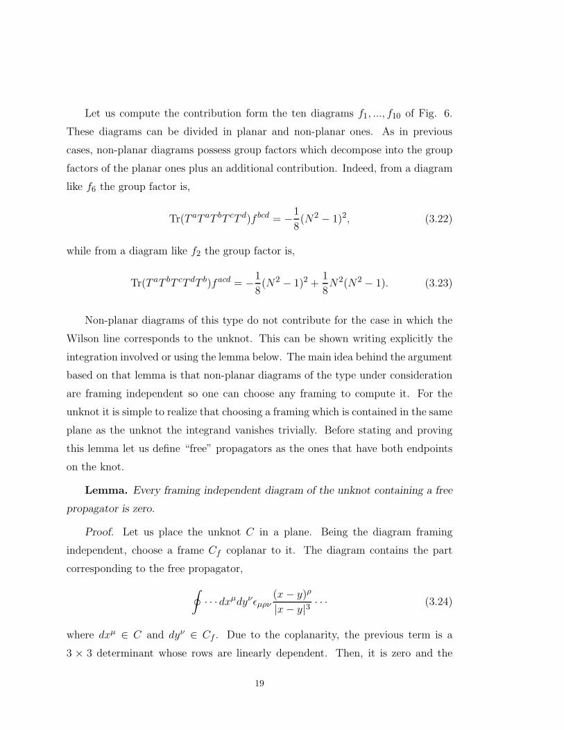
Let us compute the contribution form the ten diagrams f1, ..., f10 of Fig. 6.

These diagrams can be divided in planar and non-planar ones. As in previous

cases, non-planar diagrams possess group factors which decompose into the group

factors of the planar ones plus an additional contribution. Indeed, from a diagram

like f6 the group factor is,

Tr(T aT aT bT cT d)f bcd = −1

8(N2 − 1)2, (3.22)

while from a diagram like f2 the group factor is,

Tr(T aT bT cT dT b)facd = −1

8(N2 − 1)2 +

1

8N2(N2 − 1). (3.23)

Non-planar diagrams of this type do not contribute for the case in which the

Wilson line corresponds to the unknot. This can be shown writing explicitly the

integration involved or using the lemma below. The main idea behind the argument

based on that lemma is that non-planar diagrams of the type under consideration

are framing independent so one can choose any framing to compute it. For the

unknot it is simple to realize that choosing a framing which is contained in the same

plane as the unknot the integrand vanishes trivially. Before stating and proving

this lemma let us define “free” propagators as the ones that have both endpoints

on the knot.

Lemma. Every framing independent diagram of the unknot containing a free

propagator is zero.

Proof. Let us place the unknot C in a plane. Being the diagram framing

independent, choose a frame Cf coplanar to it. The diagram contains the part

corresponding to the free propagator,

∮

· · · dxµdyνǫµρν(x − y)ρ

|x − y|3· · · (3.24)

where dxµ ∈ C and dyν ∈ Cf . Due to the coplanarity, the previous term is a

3 × 3 determinant whose rows are linearly dependent. Then, it is zero and the

19

lemma is proved. This result is very powerful once all the framing independent

diagrams of the perturbative series expansion are identified. The theorem stated

in the next section allows to characterize very simply all those diagrams. As we

will discuss there, it turns out that those diagrams are the ones not containing

collapsible propagators. Thus, using the lemma above, we conclude that the only

non-vanishing diagrams contributing to the perturbative series expansion of the

unknot are the ones with no free propagators.

We are left with planar diagrams of type f in Fig. 5. Actually, it will be much

more convenient to consider the whole set of the ten diagrams all with the same

group factor (3.22). The reason for this is that then one can show the factorization

of the contribution into a product of contributions of the type appearing in Fig.

3 times contributions of the type b in Fig. 4. This phenomena of factorization

is general for diagrams with disconnected one-particle irreducible subdiagrams.

Indeed, in Appendix C we show the general form of the factorization theorem.

The result of applying this theorem for diagrams f1, ..., f10 of Fig. 6 is explained

as an example in Appendix C. It turns out that it can be written as the following

product:

w(f)6 =

−i

8(N2 − 1)2g6 1

4π

1

2

∮

dxα1

1

∮

dxα2

2 ǫα1α2α (x1 − x2)α|x1 − x2|3

1

64π3×

∮

dxα3

3

x3∫

dxα4

4

x4∫

dxα5

5

∫

d3zǫα3α6γǫα4α7δǫα5α8βǫα6α7α8

(z − x3)γ(z − x4)δ(z − x5)β|z − x3|3|z − x4|3|z − x5|3

,

(3.25)

i.e., a product of a linking number times ρ1,

w(f)6 =

i

32n(N2 − 1)2ρ1 = −

i

384n(N2 − 1)2. (3.26)

In obtaining (3.26) we have used (3.6), (3.8) and (3.10). This contribution is just

the first one at order 1/k3 in (1.3) after using the fact that g2 = 4π/k. This

procedure of using the lemma plus the factorization theorem of Appendix C is a

general feature of the unknot. In general, for an arbitrary knot, the factorization

20

theorem would force us to overcount diagrams giving additional contributions.

However, for the unknot all those contributions vanish.

To complete the perturbative computation at order g6 we are left with diagrams

g1, ..., g15 of Fig. 6. Again these diagrams can be divided i n planar and non-planar

ones. However, now the non-planar ones can be divided in three groups depending

on the number crossings. The group factor decomposes differently in each group.

A given diagram produces an additional group factor for each uncrossing needed

to make it planar. If the group factor of the planar diagrams, g1 to g5 is

Tr(T aT aT bT bT cT c) = −1

8N2(N2 − 1)3, (3.27)

the group factor of diagrams g6, ..., g11, which are of the first type, takes the form,

Tr(T aT aT bT cT bT c) = −1

8N2(N2 − 1)3 +

1

8(N2 − 1)2, (3.28)

where we have used simply (A1). The diagrams of the second type are g12, g13 and

g14, which similarly generate the following group factor,

Tr(T aT bT aT cT bT c) = −1

8N2(N2 − 1)3 +

1

8(N2 − 1)2 +

1

8(N2 − 1) (3.29)

Finally, diagram g15 generates,

Tr(T aT bT cT aT bT c) = −1

8N2(N2 − 1)3 +

1

8(N2 − 1)2 +

1

4(N2 − 1) (3.30)

Of all three types of group factors only the first one contributes in the case of

the unknot. To the second group factor, 18(N2 − 1)2, there are contributions from

the last 10 diagrams. Using the factorization theorem of Appendix C one finds that

this contribution is proportional to ρ2 (diagram c3 in Fig. 4) and therefore vanishes.

We have rearranged the group factors in order to get th e right weights which make

explicit the factorization of ρ2. To the third gr oup factor, 18(N2 − 1), there are

21

contributions from the last 4 diagrams wh ich can be shown explicitly to vanish for

the case of the unknot. We are left with t he first group factor, − 18N2 (N2 − 1)3.

There are contributions from all diagrams. One can use the factorization theorem

of Appendix C to write this contribution as a product of contributions of the type

shown in Fig. 3. Us ing (3.6) one then finds,

w(g)6 = −

i

384N2n3(N2 − 1)3, (3.31)

which indeed corresponds to the second contribution at order 1/k3 in (1.3). The

calculation is described in some detail as an example in Appendix C. This was

the only contribution left to be obtained from the perturbative series expansion.

The agreement found between the two results shows that the contribution from

diagram a1 of Fig. 5 must be zero. This implies that the one-particle irreducible

diagram corresponding to the two-point function must vanish at two loops.

22

4. Factorization of the framing dependence

In this section we state a theorem about the framing independence of diagrams

which do not contain one-particle irreducible subdiagrams corresponding to two-

point functions whose endpoints could get together. This theorem refers to any kind

of knot. Before stating it, some remarks are in order. Let us consider an arbitrary

diagram whose n legs are attached to n points on the knot. The resulting integral

runs over these points on the knot in a given order, i1 < i2 < · · · < in. Suppose that

our diagram has a propagator with endpoints attaching two consecutive points, say

i1 and i2. Remember that the path ordered integration will make i1→i2, and that

the propagator is singular in that case. Albeit this singularity exists, the integral

is finite but shape-dependent, as is well-known. The results for a circumference

and for an ellipse are different and then it is not a topological invariant. The way

out of this difficulty is the introduction of framings [26,1,12]. When the propagator

connects the knot and the frame, the resulting integral is the linking number of

the frame around the knot, and this is a topological invariant. This suggests that

the framing is relevant only when there are collapsible (free propagators whose

endpoints may get together upon integration) propagators. This is the idea behind

this theorem. Its statement is:

Theorem. A diagram gives a framing dependent contribution to the per-

turbative expansion of the knot if and only if it contains at least one collapsible

propagator. Moreover, the order of n in its contribution, the linking number, equals

the number of collapsible propagators.

Diagrams b and c3 of Fig. 4, e1, e2 and e3, f1 to f5, and g12 to g15 of Fig. 6

are examples of framing independent diagrams. Diagrams a, c1 and c2 of Fig. 4,

and f6 to f10, and g1 to g11 of Fig. 6 are examples of framing dependent ones.

Although we have no rigorous proof of this theorem, we do have results that

suggest its validity. Two of them are the framing independence of ρ1(C) and ρ2(C)

23

separately. The framing independence of these objects has been rigorously proven

[12,25]. As argued in the previous section, from a quantum field theory point of

view one would expect that the ambiguity present in n-point functions at coincident

points would play a role when all n points get together. Since a Wilson line consists

of a path-ordered integration, such coincident points may occur only for the case of

two-point functions (n = 2), in particular when they are collapsible. By no means

this argument provides a proof of the theorem but it makes its validity plausible.

In rigorous terms one should think of the theorem above as a conjecture. In the

rest of this section we will find further evidence regarding its validity. Assuming

that the theorem holds the following corollary follows.

Corollary. If all the contribution to the self-energy comes from one loop

diagrams, then⟨

W (C)⟩

= F (C; N) qn(N2−1)/2N where F (C; N) is framing inde-

pendent but knot dependent, and the exponential is manifestly framing dependent

but knot independent.

Proof. Let us prove this corollary first forgetting about the shift k→k + N ,

or in other words, not including loops. Let us recall that free propagators are the

ones with both endpoints on the knot. For example, diagram b of Fig. 4 does

not contain free propagators while diagrams c2 and c3 of Fig. 4 contain two free

propagators. In diagram c2 of Fig. 4 these two free propagators are collapsible.

To prove the corollary we will organize the perturbative series expansion of the

Wilson line in the following way. First, select all the diagrams which do not

contain free propagators. Let us denote by M the set of these diagrams. The

simplest diagram of this set is the one with no internal line at all, which is the

zeroth order diagram. Diagram b of Fig. 4 is the order g4 diagram in the set M.

In virtue of the theorem above the contribution of each of the diagrams in this

set is framing independent. Now take each of the diagrams of this set and dress

it with free propagators in all possible ways. Certainly, this organization exhausts

the perturbative series. The proof will consist in demonstrating that the effect of

dressing by free propagators each diagram in M is such that the contribution to

the perturbative series expansion factorizes as stated in the corollary. To be more

24

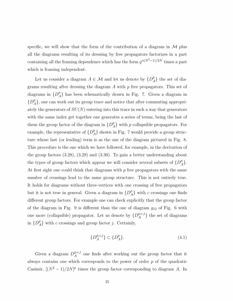
specific, we will show that the form of the contribution of a diagram in M plus

all the diagrams resulting of its dressing by free propagators factorizes in a part

containing all the framing dependence which has the form qn(N2−1)/2N times a part

which is framing independent.

Let us consider a diagram A ∈ M and let us denote by {DpA} the set of dia-

grams resulting after dressing the diagram A with p free propagators. This set of

diagrams in {DpA} has been schematically drawn in Fig. 7. Given a diagram in

{DpA}, one can work out its group trace and notice that after commuting appropri-

ately the generators of SU(N) entering into this trace in such a way that generators

with the same index get together one generates a series of terms, being the last of

them the group factor of the diagram in {DpA} with p collapsible propagators. For

example, the representative of {DpA} shown in Fig. 7 would provide a group struc-

ture whose last (or leading) term is as the one of the diagram pictured in Fig. 8.

This procedure is the one which we have followed, for example, in the derivation of

the group factors (3.28), (3.29) and (3.30). To gain a better understanding about

the types of group factors which appear we will consider several subsets of {DpA}.

At first sight one could think that diagrams with p free propagators with the same

number of crossings lead to the same group structure. This is not entirely true.

It holds for diagrams without three-vertices with one crossing of free propagators

but it is not true in general. Given a diagram in {DpA} with c crossings one finds

different group factors. For example one can check explicitly that the group factor

of the diagram in Fig. 9 is different than the one of diagram g12 of Fig. 6 with

one more (collapsible) propagator. Let us denote by {Dp,c,jA } the set of diagrams

in {DpA} with c crossings and group factor j. Certainly,

{Dp,c,jA } ⊂ {Dp

A}. (4.1)

Given a diagram Dp,c,jA one finds after working out the group factor that it

always contains one which corresponds to the power of order p of the quadratic

Casimir, [(N2 − 1)/2N ]p times the group factor corresponding to diagram A. In

25

the process one finds other group structures with lower powers. Let us concentrate

first on the group structure with the highest power. Certainly, all diagrams in

Dp,c,jA for a fixed value of p contribute to this group structure. To apply the

factorization theorem of Appendix C we need to have as many diagrams as domains.

As shown at the end of Appendix C, if diagram A is connected the difference

between the number of domains and the number of diagrams comes about because

while diagrams with ni identical subdiagrams count as one, from the point of view

of domains they should count as ni! to have the adequate relabelings to be in the

hypothesis of the factorization theorem. Thus, for the case in which A is connected

one just has to repeat p! times the diagrams and make the adequate relabelings

to be in hypothesis of the factorization theorem. Of course, this implies that one

must divide the result of the theorem by p!. For A connected the contribution

corresponding to the group structure [(N2 −1)/2N ]p from all diagrams in {Dp,c,jA }

is,

1

p!

np

2p(ig2)p

(N2 − 1

2N

)pDA =

1

p!

(

in2π

k

N2 − 1

2N

)pDA, (4.2)

where the factor 2p appears after enlarging the integral of each propagator to the

whol e knot (which provides the factor np, where n is the winding number (3.5)).

Notice that in (4.2) DA represents the contribution from diagram A, which is

framing independent, and that we have used (2.5). Notice also that after summing

in p (4.2) gives the form stated for the Wilson line in the corollary. However, this is

not the only framing dependent contribution. One certainly has more contributions

with other group structures. Also, one has to discuss the situation in which A is

not connected. We will consider that situation later.

To the next group structure (next to leading) not all the diagrams in Dp,c,jA

contribute. Indeed, only diagrams with c > 0 do. There are, however, diagrams

which contribute and are framing dependent so we have to work out this depen-

dence. For example, diagrams g6 to g11 of Fig. 6 ar e framing dependent. One

would like to have enough diagrams to be able to use the factorization theorem of

Appendix C and factorize the contribution as the one from diagram A with one

26

crossing of free propagators, which is framing independent, times the contribution

due to p− 2 collapsible propagators which i s framing dependent and proportional

to n(p−2). To explain how one must arrange the perturbative series to extract the

effect of the framing we will consider first in some detail the case corresponding

to diagrams g6 to g11 of Fig. 6. This is a particular case in which p = 3 and A is

trivial but it possesses the essential features in which we will focus our attention

in the general proof.

Diagrams g1 to g15 of Fig. 6 contribute to the group structures worked out in

(3.27), (3.28), (3.29) and (3.30). All fifteen diagrams g1 to g15 shown in Fig. 6

contribute to the group structure −(N2 − 1)3/8N2. It corresponds to the general

case which led to (4.2). We will describe it in this example for completeness. The

contribution to this group structure can be written as follows:

I3 =

∮

i<j<k<l<m<n

[

f(ij, kl, mn) + f(ij, km, ln) + f(ij, kn, lm) + f(ik, jl, mn)

+ f(ik, jm, ln) + f(ik, jn, lm) + f(il, jk, mn) + f(il, jm, kn)

+ f(il, jn, km) + f(im, jk, ln) + f(im, jl, kn) + f(im, jn, kl)

+ f(in, jk, lm) + f(in, jl, km) + f(in, jm, kl)]

(4.3)

We have use a notation in which i, j, k, l, m, n represent the six points attached

to the knot and f(ij, kl, mn) the corresponding integrand. As explained, not all

possible domains are represented in (4.3). One possesses 90 domains while there

are only 15 diagrams. The ratio between these two numbers is just 3!, the number

of possible orderings of the three free propagators which from the point of view of

domains should be different. Introducing all the relabelings needed to apply the

factorization theorem of Appendix C one must therefore divide by 3!. The result

is,

I3 =1

6

∮

i<j

∮

k<l

∮

m<n

p(i, j) p(k, l) p(m, n), (4.4)

where p(i, j) represents the integrand corresponding to a free propagators with its

27

endpoints i and j attached to the knot. The linking number n appears when we

let the endpoints of each propagator go freely over the knot and the frame, and

multiply by 1/2 per propagator. This provides the additional factor (1/2)3 = 1/8.

The result, in agreement with (4.2) is,

I3 =n3

3!23. (4.5)

The diagrams contributing to the next group structure, are g6 to g15 of Fig. 6,

and in order to apply the factorization theorem we need to have 15 diagrams since

that is the number of domains. Therefore, we have to overcount some of them.

Notice that now one of the subdiagrams is a free propagator while the other is c3

of Fig. 4, which is not connected. We can not apply the simple strategy described

at the end of Appendix C. The number of domains is different than the number

of diagrams because in diagrams like g12, g13 and g14 one has two possible choices

of domains while in diagrams g15 one has three. Thus let us add what we need,

i.e., let us consider two diagrams of types g12, g13 and g14 and make the apropiate

relabelings in one of each pair, and 3 diagrams of type g15 and make relabelings in

two of them. Certainly, we must subtract what we have added. Now one can not

just simply divide by a factor. We need therefore to subtract once diagrams g12,

g13 and g14 and twice diagram g15. These diagrams are framing independent and

therefore they do not contribute to the framing dependent part. In the general

proof, at this stage, the diagrams which one must subtract contribute to a lower

power of n. Therefore, we may use the algorithm safely power by power. Using

our previous notation, the contribution to the next group structure, 18 [N2 − 1]2 is,

28

I1 =

∮

i<j<k<l<m<n

[

f(ij, km, ln) + f(jk, ln, mi) + f(kl, jn, im) + f(lm, ik, jn)

+ f(mn, ik, jl) + f(ni, jl, km) + f(ik, jm, ln) + f(im, jl, kn)

+ f(il, jn, km) + f(il, jm, kn)]

=

(∮

i<j<k<l<m<n

+

∮

k<i<j<l<m<n

+

∮

k<l<i<j<m<n

+

∮

k<l<m<i<j<n

+

∮

k<l<m<n<i<j

+

∮

i<k<l<m<n<j

+

∮

i<k<j<l<m<n

+

∮

i<k<l<m<j<n

+

∮

k<i<l<m<n<j

+

∮

i<k<l<j<m<n

)

f(ij, km, ln),

(4.6)

which, after adding single replicas for the integrands corresponding t o g12, g13 and

g14 and double ones for g15, using statement 1 of Appendix C, and making the

relabelings,

σ7 =

(

1 2 3 4 5 6

3 4 5 1 6 2

)

σ8 =

(

1 2 3 4 5 6

3 1 4 2 5 6

)

σ9 =

(

1 2 3 4 5 6

3 4 1 5 2 6

)

σ10 =

(

1 2 3 4 5 6

3 1 4 5 2 6

)

σ′

10 =

(

1 2 3 4 5 6

3 4 1 5 6 2

)

one finds,

I1 = I1 − I1, (4.7)

where,

29

I1 =

(∮

i<j<k<l<m<n

+

∮

i<k<j<l<m<n

+

∮

i<k<l<j<m<n

+

∮

i<k<l<m<j<n

+

∮

i<k<l<m<n<j

+

∮

k<i<j<l<m<n

+

∮

k<i<l<j<m<n

+

∮

k<i<l<m<j<n

+

∮

k<i<l<m<n<j

+

∮

k<l<i<j<m<n

+

∮

k<l<i<m<j<n

+

∮

k<l<i<m<n<j

+

∮

k<l<m<i<j<n

+

∮

k<l<m<i<n<j

+

∮

k<l<m<n<i<j

)

f(ij, km, ln)

=

∮

i<j

p(i, j)

∮

k<l<m<n

f2(kl, mn).

(4.8)

and,

I1 =

(∮

k<l<i<m<j<n

+

∮

k<l<i<m<n<j

+

∮

k<l<m<i<j<n

+

∮

k<l<m<i<n<j

+

∮

k<l<m<n<i<j

)

f(ij, km, ln).

(4.9)

In (4.8), the quantity f2 is the integrand corresponding to diagram c3 of Fig. 4.

After integration, it results the quantity ρ2 in (3.13). The contributions remaining

to the next group structures plus the left over represented by (4.9) are framing

independent. This means that we have extracted all the framing dependence from

the set of diagrams g1 to g15 of Fig. 6. Using (4.5) and (4.8) we can write such a

contribution as

−1

8N2(N2 − 1)3

n3

3!23+

1

8(N2 − 1)2

n

2

= −N

8

1

3!

((N2 − 1)n

2N

)3+

N

8(N2 − 1)

1

1!

(N2 − 1

2N

)1ρ2

(4.10)

In the second line of this equation we have rewritten the contribution to show the

general structure which we will find out now.

30

Let us discuss which one is the algorithm to arrange the perturbative series

expansion to extract the framing dependence for the group structure next to the

leading one. In the example considered we have seen that diagrams contributing to

this type of group structure were g6 to g15 of Fig. 6. Certainly, these were not all

the 15 diagrams which were needed to use the factorization theorem and factorize

the contribution to the group factor (N2 − 1) as a product of a diagram like the

one in Fig. 3 times the one originating ρ2 (diagram c3 of Fig. 4). However, we

were able to add pieces of diagrams with the adequate group structure with two

or more crossings (which one must subtract when considering the situation leading

to a factorization of diagrams with two crossings) to have the 15 needed and apply

the factorization theorem of Appendix C. Clearly, this is the procedure which one

must carry out when considering the next to the leading group structure. One adds

pieces of diagrams to complete the set in such a way that the factorization theorem

of Appendix C can be applied, and, on the other hand one subtracts them. The

important point is that all diagrams which are involved in this operation contain a

lower power of n, the linking number, and therefore, in the process one extracts all

the framing dependence for the next to leading group structure. The corresponding

contribution from all the diagrams in Dp,c,jA for a fixed value of p is,

1

(p − 2)!

n(p−2)

2(p−2)(ig2)(p−2)

(N2 − 1

2N

)(p−2)D

(1,i)A =

1

(p − 2)!

(

in2π

k

N2 − 1

2N

)(p−2)D

(1,i)A ,

(4.11)

where the origin of each factor is similar to the case of (4.2) and D(1,i)A is one of

the possible types of diagrams resulting after dressing diagram A with two free

propagators with one crossing. In Fig. 10 a particular situation of (4.11) has been

depicted.

One has now to analyze the next group structure. In this case one has to take

into consideration all the left-overs from the previous one. Certainly, this is going

to change the numerical factor in front of this contribution but once this is taken

into account one may proceed similarly as the previous case. It is clear now that

one may proceed performing this construction for a fixed value of p with all types

31

which appear at each value of c. The result that one obtains in this way is,

1

p!

(

in2π

k

N2 − 1

2N

)pDA +

(p

2)∑

c=1

nc∑

i=1

1

(p − c − 1)!

(

in2π

k

N2 − 1

2N

)(p−c−1)D

(c,i)A , (4.12)

where nc is the number of types which one finds at c crossings, and we have used

the fact that for the case of p free propagators the maximum number of possible

crossings is(p2

)

. It is important to remark that the coefficients DA, D(c,i)A , which

appear in (4.12) are framing independent. In (4.12) we have singled out all the

framing dependence at a given order of free propagators for a diagram A ∈ M.

Summing over p one obtains the anticipated exponential behavior:

(DA +∞∑

c=1

nc∑

i=1

D(c,i)A ) exp

(1

2ing2N2 − 1

2N

)

= (DA +∞∑

c=1

nc∑

i=1

D(c,i)A )qnN2

−12N , (4.13)

where we have used (2.5) and (1.2). Therefore the corollary is proven.

As this exponential is a common factor, the sum of the perturbative series

factorizes as the sum of all diagrams without collapsible propagators (framing

independent, but knot dependent) multiplied by some adequate coefficients times

the preceding exponential (manifestly framing dependent). Note that this factor

does not depend on the kind of knot because the Gauss integral only sees the

linking number. Also is interesting to note that the framing independent and

knot dependent factor is intrinsic to the knot and then includes all the diagrams

that give the building blocks of its topological invariants. This is schematically

represented in Fig. 11.

All along our discussion regarding the proof of the corollary we have assumed

that A was a connected diagram. Let us remove now that fact. If A is not connected

it is clear that one can use the technic of adding and removing pieces of diagrams to

apply the factorization theorem at each stage of the proof described for the case in

which A was connected. This will introduce some numerical factors in (4.13) which

are important in what regards the building blocks of the knot, but are irrelevant

32

for the framing dependence since the exponential behavior has been shown for each

term.

Finally we have to include the shift k→k + N . Assuming that diagrams with

more than one loop do not contribute to the self-energy, we have to factorize prop-

agators with and without self-energy insertions, and then sum the resulting series.

Remember again that the rest of the diagrams add up to a framing independent

and knot dependent factor.

This series is hard to manage because there can be any number of self-energy

insertions at each propagator, and any number of propagators. The best organi-

zation is as follows: call {Dqp} the set of diagrams with p propagators in which we

have inserted q self-energies in all the possible ways, and f(n), the sum of all of

them, which is the framing dependent and knot independent factor in⟨

W (C)⟩

.

Notice that,

f(n) =∞∑

p=0

∞∑

q=0

{Dqp}. (4.14)

The important point to use here is that the distribution of self-energies is such

that they are indistinguishable. The number of possible distributions of q identical

insertions in p lines is a Bose-Einstein combinatory factor. The lines in which we

insert self-energies are also indistinguishable. For example, insertions done in sets

of diagrams as the ones in Fig. 7 introduces a factor 1/p!. Therefore, the prefactor

of {Dqp} is

1

p!

(

p + q − 1

q

)

. (4.15)

Now, each insertion amounts to a factor −N/k (k = 4π/g2), and each line to a

factor x/k (x = in2π(N2 − 1)/2N). Hence,

f(n) =

∞∑

p=0

∞∑

q=0

1

p!

(

p + q − 1

q

)(

x

k

)p(−N

k

)q

. (4.16)

33

This series in q is the expansion of a factor that provides the shift:

(

1 +N

k

)−p

=∞∑

q=0

(

p + q − 1

q

)(

−N

k

)q

, (4.17)

and therefore, the final result is

f(n) =∞∑

p=0

1

p!

(

x

k

)p(

1 +N

k

)−p

= ein2π(N2

−1)2N

1k+N = qnN2

−12N , (4.18)

where we have used (1.2). This proof also works in the other way around. Suppose

that two-loop diagrams also contribute. These are identical among themselves,

but distinguishable from the one loop insertions, and so there must appear two

“bosonic” combinatory factors. The sum of this series has to be different from the

shifted exponential, because expanding the exponential with shift we find just one

bosonic combinatory factor. Then, the exact result implies that the only quantum

corrections relevant to the framing dependent part are the one-loop self-energies.

This corollary shows from a perturbation theory point of view that all depen-

dence on the framing in the vacuum expectation value of a knot factorizes in the

form predicted by Witten [1]. Notice also that assuming that there are only one-

loop quantum corrections, we have found for an arbitrary knot in the fundamental

representation of SU(N) the shift in the framing dependent factor of the Wilson

Line through a purely perturbative approach.

We have proved that the effect of one-loop contributions on the framing depen-

dent factorized part of the vacuum expectation value is just a shift in k. Certainly,

this is going to hold also for the rest. This, together with the factorization of the

framing dependence means that we can write from (1.1) the full contribution from

the building blocks or diagrams in M with no loop insertions. One just has to set

n = 0 in (1.1) and remove the shift.

34

5. Conclusion and final remarks

In this paper we have shown that agreement between the exact result found

by Witten [1] for the vacuum expectation value of the unknot and the Chern-

Simons perturbative series expansion implies that the two-loop contribution to

the one-particle irreducible two-point function must vanishes. We have worked

within a renormalization scheme which is gauge invariant and which provides a

one loop correction to the two and three-point functions which, as shown here, is

responsible for the shift of k into k+N observed in [1]. Consistency with the exact

result implies that the two-loop contribution in renormalization schemes providing

quantum corrections at one loop must vanish. Work is under completion regarding

this issue [28] for the renormalization scheme proposed in sect. 2 of this paper.

Our analysis of the structure of the series expansion which appears in the

perturbative calculation of the vacuum expectation value of Wilson lines shows

that in general one can disentangle the framing dependence from the rest of the

contribution. We have shown that under the assumption that the theorem stated

in sect. 4 holds, the framing dependence of the vacuum expectation value of Wilson

lines factorizes in the form predicted in [1]. We have shown this for a Wilson line

carrying the fundamental representation of SU(N) but it is clear from the proof

that similar arguments hold for any other representation. Although a rigorous

proof of the theorem (conjecture) stated in sect. 4 would be very valuable to

make our discussion on the factorization of the framing dependence complete, the

arguments based on physical grounds utilized in sect. 3 make the validity of this

conjecture rather plausible.

It is important to remark that the factorization theorem proved in Appendix C

has played an essential role in the factorization of the framing dependence achieved

in sect. 4, as well as in the explicit calculation of the vacuum expectation value of

the unknot in the fundamental representation at order g6. In general, this theorem

decreases th e number of integrations needed at a given order by one, reducing the

computation to just the building blocks of the perturbative expansion.

35

The study carried out in sect. 4 to extract the framing dependence out of the

perturbative series expansions of the vacuum expectation value of a Wilson line

has also provided information about the building blocks of the perturbative series

expansion. Presumably, these building blocks generate a whole series of topological

invariants whose integral form is easy to write down using the Feynman rules of the

theory. Certainly, these building blocks are framing independent since, according

to the corollary of sect. 4, all framing dependence has been factorized out. To

prove their topological invariance is much harder and it may well happen that at a

given order in g not all the building blocks by themselves are topological invariants

but adequate combinations of them. It would be desirable to have some general

result in this respect.

In this paper we have carried out an explicit calculation of the vacuum ex-

pectation value of the unknot in the fundamental representation of SU(N) up to

order g6. It is straightforward to generalize this calculation to any other represen-

tation. One would like, however, to analyze the case of a non-trivial knot to verify

if the same conclusion holds and to compute some of its building blocks. Chern-

Simons theory provides a whole series of topological invariants whose integral form

is simple (but tedious) to write down, which would be interesting to classify and

characterize. For example, one would like to know if the degree of complexity of a

knot is related to the number of building blocks which are different from zero. For

the case of the unknot we have that the lemma of sect. 3 plus the theorem of sect.

4 imply that its building blocks are diagrams which do not contain free propaga-

tors. The quantity ρ1 defined in (3.10) is the first non-trivial building block. It

is represented by diagram b of Fig. 4. The building blocks of the unknot at next

order are represented by diagrams e1, e2 and e3 of Fig. 6. As shown in sect. 3

together with Appendix B the contribution from these diagrams vanishes. There-

fore, the next possibly non-vanishing building blocks for the unknot corresponds

to diagrams containing two three-vertices with all their legs attached to the Wil-

son line (a representative is diagram a of Fig. 12) and diagrams containing three

three-vertices (a representative is diagram b of Fig. 12). The contribution from

36

these building blocks should be computed and compared to the exact result. As

argued at the end of Appendix B, all building blocks of the unknot corresponding

to connected tree-level diagrams with an even number of vertices vanish. This is

in agreement with the full result (1.1). From (1.1), as explained at the end of sect.

4, it is rather simple to obtain the contribution from the building blocks. One has

just to set n = 0 and remove the shift. The remaining series is clearly even in 1/k

which implies that only terms at order g4m are different from zero, in agreement

with the observation made at the end of Appendix B.

In this work we have shown how to extract from the perturbative series ex-

pansion of knots in Chern-Simons theory their framing dependence as well as the

effect of quantum corrections. This leaves the series with the essential ingredients

which we have called building blocks and contain all t he topological information.

Further work is needed to study the general features and the classification of these

building blocks.

37

APPENDIX A

In this appendix we present a summary of our group-theoretical conventions.

We choose the generators of SU(N), T a, a = 1, ..., N2 − 1, to be antihermitian

such that

[T a, T b] = −fabcT c, (A.1)

and fabc are completely antisymmetric, satisfying,

facdf bcd = Nδab. (A.2)

The convention chosen in (A.1) seems unusual but it is the right one when the

Wilson line is defined as in (3.1). If we had chosen ifabc instead of −fabc, the

exponential of the Wilson line would have had ig instead of g. Our convention

also introduces a −1 in the vertex (see Fig. 1). The fundamental representation

of SU(N) is normalized in such a way that,

Tr(T aT b) = −1

2δab. (A.3)

The quadratic Casimir in the fundamental representation has the form,

N2−1∑

a=1

T aT a = −N2 − 1

2N. (A.4)

One of the group factors which appear in subsect. 3.3 of the paper is the following,

Tr(T aT bT cT d)facef ebd, (A.5)

which can be shown to be zero. In fact, using the invariance of the trace under

cyclic permutations one finds, after relabeling,

Tr(T aT bT cT d)facef ebd = Tr(T bT cT dT a)facef ebd = Tr(T aT bT cT d)fdbef eac,

(A.6)

which is just the same as (A.5) but with the opposite sign. Therefore,

Tr(T aT bT cT d)facef ebd = 0. (A.7)

38

APPENDIX B

In this appendix we show that the contribution from diagrams e1 or e2 of Fig.

6 vanishes for the case of the unknot. These are the integrals that appear in the

four-point g6 contribution to the unknot, represented in diagrams e1, e2 and e3

of Fig. 6. The idea of the calculation is as follows. According to the framing

independence theorem of sect. 4, each diagram is framing independent, so we can

think that the four points are all in the unknot. Also we assume that it corresponds

to a topological invariant and therefore we choose the unknot to be a circumference

on the x0 = 0 plane, centered at the origin. Call p and q the points of integration

over R3 ⊗ R3. Now observe that the integrand contains an odd number of ǫαβγ

contracted in such a way that it is a pseudoscalar. Its sign is different in the

x0 > 0 and x0 < 0 regions. In other words, for each (p, q) ∈ R3 ⊗ R3 there

are (p′, q′) ∈ R3 ⊗ R3 such that p′0 = −p0, q′0 = −q0 and all other components

unchanged, for which the integrands are equal in magnitude but different in sign.

Then, in the p0, q0 plane we have and odd integrand and so the integral vanishes.

Let us verify this explicitly.

The integrations entering this contribution are of the type,

∫

d3p d3q ǫµρ1ν1dxµ (x − p)ρ1

|x − p|3ǫνρ2ν2dyν (y − p)ρ2

|y − p|3ǫν1ν2τ1ǫρρ3ν3dzρ (z − q)ρ3

|z − q|3

ǫτρ4ν4dwτ (w − q)ρ4

|w − q|3ǫν3ν4τ2ǫτ1τ2ρ5

(p − q)ρ5

|p − q|3,

(B.1)

where x, y, z, w lie on the knot and hence x0 = y0 = z0 = w0 = 0. The denominator

of the integrand of this expression is invariant under p0, q0→− p0,−q0. The struc-

ture of the numerator is more complicated and we will consider its form separately.

The first three factors of the numerator of (B.1) become,

ǫ1ρ1ν1dx1(x − p)ρ1 + ǫ2ρ1ν1dx2(x − p)ρ1

= ǫ10ν1dx1(x − p)0 + ǫ12ν1dx1(x − p)2 + ǫ20ν1dx2(x − p)0 + ǫ21ν1dx2(x − p)1.(B.2)

39

The following three factors give an analogous contribution,

ǫ1ρ1ν2dy1(y − p)ρ1 + ǫ2ρ1ν2dy2(y − p)ρ1

= ǫ10ν2dy1(y − p)0 + ǫ12ν2dy1(y − p)2 + ǫ20ν2dy2(y − p)0 + ǫ21ν2dy2(y − p)1,(B.3)

which becomes (B.2) after changing y→x and ν2→ν1. Contracting (B.2) and (B.3)

with ǫν1ν2τ one obtains,

ǫ20τ1

[

dx1p0dy1(y − p)2 − dx1p0dy2(y − p)1 − dx1(x − p)2dy1p0 + dx2(x − p)1dy1p0]

−ǫ01τ1

[

dx1p0dy2(x − p)2 − dx2p0dy1(y − p)2 + dx2(y − p)1dy2p0 − dx2(x − p)1dy2p0]

+ǫ21τ1

[

−dx1(p0)2dy2 + dx2(p0)2dy1]

.(B.4)

The rest of the factors in (B.1) except the last two are treated similarly, obtain-

ing an expression similar to (B.4) with x→z, y→w, p→q, and τ1→τ2. Finally,

multiplying (B.4) by the remaining factor of (B.1), ǫτ1τ2ρ5(p − q)ρ5,one gets,

− p0q20(p − q)2

[

· · ·]

+ p0q0(p − q)0[

· · ·]

− q0p20(p − q)2

[

· · ·]

− q0p20(p − q)1

[

· · ·]

+ p0q0(p − q)0[

· · ·]

− p0q20(p − q)1

[

· · ·]

,(B.5)

where by[

· · ·]

it is meant a part that does not depend on p0 or q0. As argued

above, this expression is odd under p0, q0→−p0,−q0 and therefore the integration

over p0, q0 in (B.1) vanishes. This way of showing the vanishing of integrations

as (B.1) suggests that this property is a general feature of tree level connected

diagrams with an even (and non zero) number of R3 points of integration. As we

discuss in sect. 5, this assertion is substantiated by the full result (1.1).

40

APPENDIX C

In this appendix we state and prove the factorization theorem. First, let us

introduce some notation. We will be considering diagrams corresponding to a given

order g2m in the perturbative expansion of a knot, and to a given number of points

running over it, namely n. Note that n and m fix the number of vertices, nv, and

propagators, np, that are in each diagram: nv = 2m−n and np = 3m−n. We will

denote by {i1, i2, . . . , in} a domain of integration where the order of integration is

i1 < i2 < ... < in, being i1, i2, . . . , in the points on the knot (notice the condensed

notation) where the internal lines of the diagram are attached. The integrand

corresponding to that diagram will be denoted as f(i1, i2, . . . , in). Diagrams are in

general composed of subdiagrams, which may be connected or non-connected. For

a given diagram we will make specific choices of subdiagrams depending on the

type of factorization which is intended to achieve. For example, for a diagram like

g6 of Fig. 6 one may choose as subdiagrams the three free propagators, or one may

choose a subdiagram to be the collapsible propagator and other subdiagram to be

the one built by two crossed free propagators. We will consider a set of diagrams N

corresponding to a given order g2m, to given number of points attached to the knot,

n, and to a given kind. By kind we mean all diagrams containing ni subdiagrams of

type i, i = 1, ..., T . By pi we will denote the number of points which a subdiagram

of type i has attached to the knot. For example, if one considers diagrams at order

g6 with n = 6 points attached to the knot, with three subdiagrams which are just

free propagators, this set is made out of diagrams g1 to g15 of Fig. 6. However, if

one considers diagrams at order g6 with n = 6 with a subdiagram consisting of a

free propagator and another subdiagram of the type c3 of Fig. 4, this set is made

out of diagrams g6 to g15. The contribution from all diagrams in N can be written

as the following sum:

∑

σ∈Πn

∮

i1,i2,...,in

f(iσ(1), iσ(2), . . . , iσ(n)) (C.1)

where σ ∈ Πn, being Πn ⊂ Pn a subset of the symmetric group of n elements.

41

Notice that Πn reflects the different shapes of the diagrams in N . In (C.1) the

integration region has been left fixed for all the diagrams and one has introduced

different integrands. One could have taken the opposite choice, namely, one could

have left fixed the integrand and sum over the different domains associated to N .

The first statement regarding the factorization theorem just refers to these two

possible choices. Let us define the domain resulting of permuting {i1, i2, . . . , in}

by an element σ of the symmetric group Pn by

dσ = { iσ(1), iσ(2), . . . , iσ(n) }, (C.2)

then the following result immediately follows.

Statement 1. The contribution to the Wilson line of the sum of diagrams

whose integrands are of the form:

f(iσ(1), iσ(2), . . . , iσ(n)), (C.3)

where σ runs over a given subset Πn ∈ Pn with a common domain of integration

is equal to the sum of the integral of f(i1, i2, . . . , in) over dσ where σ ∈ Π−1n :

∮

i1,i2,...,in

∑

σ∈Πn

f(iσ(1), iσ(2), . . . , iσ(n)) =∑

σ∈Π−1n

∮

dσ

f(i1, i2, . . . , in). (C.4)

The idea behind the factorization theorem is to organize the diagrams in N in

such a way that one is summing over all possible permutations of domains. Sum-

ming over all domains implies that one can consider the integration over the points

corresponding to each subdiagram as independent and therefore one can factorize

the contribution into a product given by the integrations of each subdiagram in-

dependently. Our aim in the rest of this appendix will be to prove the following

statement.

42

Statement 2. (Factorization theorem) Let Π′

n be the set of all possible per-

mutations of the domains of integration of diagrams containing subdiagrams of

types i = 1, ..., T. If Π−1n = Π′

n, the sum of integrals over dσ, σ ∈ Π−1n , is the

product of the integrals of the subdiagrams over the knot, being the domains all

independent,

∑

σ∈Π−1n

∮

dσ

f(i1, . . . , in) =T∏

i=1

(∮

i1,...,ipi

fi(i1, . . . , ipi)

)ni

, (C.5)

In (C.5) ni denotes the number of subdiagram of type i and pi its number of points

attached to the knot.

The proof of this statement is trivial since having all possible domains it is

clear that one can write the integration considering subdiagram by subdiagram,

the result being the product of all the partial integrations over subdiagrams.

In sect. 4 we considered situations where we were forced to add and sub-

tract pieces of diagrams in such a way that the theorem above was utilized. For

completeness, we will show now that for the case in which all subdiagrams are

connected the overcounting needed to apply the theorem is very simple and that

it just amount to divide by an adequate combinatory factor. Let us discuss first

an example to understand the strategy leading to the general situation.

Let us consider the four point g4 contribution or, better to say, its part with

(N2 − 1)2/4N as SU(N) factor. The diagrams are c1, c2 and c3 of Fig. 4, whose

contribution can be written according to Statement 1, is,

∮

i1<...<i4

[

f(i1, i2, i3, i4) + f(i1, i3, i2, i4) + f(i1, i4, i2, i3)]

=

(∮

i1<i2<i3<i4

+

∮

i1<i3<i2<i4

+

∮

i1<i3<i4<i2

)

p(i1, i2) p(i3, i4),

(C.6)

where p(i1, i2) represents a free propagator attached to the knot at points i1 and

i2. There are no more than three diagrams, and the number of domains is six.

43

These are:

i1 < i2 < i3 < i4

i1 < i3 < i2 < i4

i1 < i3 < i4 < i2

i3 < i1 < i2 < i4

i3 < i1 < i4 < i2

i3 < i4 < i1 < i2

(C.7)

so we need three more diagrams. Now the overcounting consists of rewriting the

diagrams after a relabeling. In the course of the relabeling we will use the fact that

p(i1, i2) = p(i2, i1). The relabelings needed in the overcounting are the following:

σ1 =

(

1 2 3 4

3 4 1 2

)

σ2 =

(

1 2 3 4

3 1 4 2

)

σ3 =

(

1 2 3 4

3 1 2 4

)

(C.8)

Here the subindex of each σ indicates the integrand over which it acts. Note also

that each relabeling is in fact a repetition of the diagram, due to the symmetry of

the propagator pointed out above. Therefore, all we have to do is to multiply the

sum of the six terms by 1/2. The new integrands are:

σ1[f(i1, i2, i3, i4)] =f(i3, i4, i1, i2) = f(i1, i2, i3, i4),

σ2[f(i1, i3, i2, i4)] =f(i3, i4, i1, i2) = f(i1, i2, i3, i4),

σ3[f(i1, i4, i2, i3)] =f(i3, i4, i1, i2) = f(i1, i2, i3, i4),

(C.9)

and the result is:

∮

i1<...<i4

[

f(i1, i2, i3, i4) + f(i1, i3, i2, i4) + f(i1, i4, i2, i3)]

=1

2

(∮

i1<i2<i3<i4

+

∮

i1<i3<i2<i4

+

∮

i1<i3<i4<i2

+

∮

i3<i1<i2<i4

+

∮

i3<i1<i4<i2

+

∮

i3<i4<i1<i2

)

p(i1, i2) p(i3, i4).

(C.10)

Now, in the language of the theorem, Π−14 = Π′

4, i.e., each propagator runs freely

44

over the knot and therefore we obtain,∮

i1<...<i4

[

f(i1, i2, i3, i4)+f(i1, i3, i2, i4)+f(i1, i4, i2, i3)]

=1

2

∮

i1<i2

∮

i3<i4

p(i1, i2) p(i3, i4).

(C.11)

The linking number of the frame and the knot arises as an integral of a propagator

with one of its endpoints running over the knot and the other over the frame,

without any ordering. This is easily achieved in the integrals we have by simply

leaving i1 and i2 free, and multiplying by 1/2. The same should be done for the

pair i3 and i4. This is again an example of factorization. The final 1/8 is the factor

3/4! that appears for w(c)4 in (3.14).

The example suggests the idea of a general proof. We should count the number

of domains and the number of diagrams and observe their relation, as well as the

origin of their difference. We are able to provide formulae for the number of do-

mains for an arbitrary diagram. However, our formula for the number of diagrams

in terms of the features of their subdiagrams only holds when all subdiagrams

are connected. Using these formulae we will show that we can make equivalent

the overcounting and the original contribution simply introducing a combinatory

factor.

First, let us compute the number of domains, d′, corresponding to a general set

of diagrams at a given order in the perturbative expansion of the knot, to the same

number of points on the knot, and to the same types of subdiagrams. Suppose

that we construct the diagram adding its sudiagrams in a given order. The first

one can put its pi points in n places. The second one has to distribute its points in

the remaining n − pi, and so on. For example, if there are only a points attached

by propagators and b points attached by three-vertices (and so n = 2a + 3b),

d′ =

(

n

2

)(

n − 2

2

)(

n − 4

2

)

. . .

(

n − 2a + 2

2

)(

n − 2a

3

)(

n − 2a − 3

3

)

. . .

. . .

(

n − 2a − 3b + 3

3

)

=n!

(2!)a(3!)b.

(C.12)

In general the denominator will include the product of every pi!, where pi denotes

45

the number of points attached to the knot corresponding to a subdiagram of type i.

If we denote by d the number of diagrams of the set under consideration, it is clear

that d ≤ d′ due to the possible identity of some subdiagrams. In those cases we have

to divide d′ by the number of permutations of all the identical subdiagrams. If some

of the subdiagrams were not connected we would have to consider additional factors

which would imply to introduce more data about each subdiagram. Therefore, let

us restrict ourselves to the case of connected subdiagrams. The final form of the

formulae is:

d′ =n!

∏ki=1(pi!)ni

, d =n!

∏ki=1 ni!(pi!)ni

. (C.13)

The relation between d and d′ is always an integer:

d′

d=

k∏

i=1

ni! (C.14)

This is the combinatory factor we were searching for. Therefore, when the subdi-

agrams are connected one just has to overcount evenly each diagram to have as

many diagrams as domains and divide by (C.14). For non-connected subdiagrams

the previous formula for d fails. An example is the factorization of ρ2(C) in the

18(N2 − 1)2 part of diagrams g6, . . . , g15 of Fig. 6. The subdiagram that we would

factorize is the corresponding to diagram c3 of Fig. 4, which is not connected. The

previous formula gives d = d′ = 15, exactly the same result as if the subdiagram

were e1 or e2 of Fig. 6, but there are just 10 diagrams. The number of domains,

however, is correct.

46

FIGURE CAPTIONS

1) Basic Feynman rules of the theory.

2) Two-point function and three-point function at one loop.

3) Diagrams corresponding to g2. Thick lines represent the Wilson line while

thin lines refer to Feynman diagrams.

4) Diagrams corresponding to g4.

5) Part of the diagrams corresponding to g6.

6) Rest of diagrams corresponding to g6.

7) A general set of diagrams with p propagators in the knot

8) The less crossed diagram of Fig. 7.

9) A framing independent diagram.

10) Factorization of ρ2

11) Factorization of the framing dependence.

12) Diagrams at order g8 corresponding to building blocks

47

REFERENCES

1. E. Witten, Comm. Math. Phys. 121(1989), 351

2. M. Bos and V.P. Nair, Phys. Lett. B223(1989), 61, Int. J. Mod.

Phys. A5(1990), 959

3. H. Murayama, “Explicit Quantization of the Chern-Simons Action”, Univer-

sity of Tokyo preprint, UT-542, March 1989

4. J.M.F. Labastida and A.V. Ramallo, Phys. Lett. B227(1989), 92, Phys.

Lett. B228(1989), 214

5. S. Elitzur, G. Moore, A. Schwimmer and N. Seiberg, Nucl.

Phys. B326(1989), 108

6. J. Frohlich and C. King, Comm. Math. Phys. 126(1989), 167

7. G.V. Dunne, R. Jackiw, and C.A. Trugenberger, Ann. Phys. 194(1989), 197

8. S. Axelrod, S. Della Pietra and E. Witten, J. Diff. Geom. 33 (1991) 787

9. J.M.F. Labastida, P.M. Llatas and A.V. Ramallo, Nucl. Phys. B348(1991),

651

10. K. Gawedzki and A. Kupiainen, Comm. Math. Phys. 135(1991), 531

11. G. Moore and N. Seiberg, Phys. Lett. B220(1989), 422

12. E. Guadagnini, M. Martellini and M. Mintchev, Phys. Lett. B227(1989),

111, Phys. Lett. B228(1989), 489, Nucl. Phys. B330(1990), 575

13. L. Alvarez-Gaume, J.M.F. Labastida, and A.V. Ramallo, Nucl.

Phys. B334(1990), 103, Nucl. Phys. B (Proc. Suppl.) 18B (1990) 1

14. R.D. Prisarski and S. Rao, Phys. Rev. D22(1985), 208

15. D. Birmingham, M. Rakowski and G. Thompson, Nucl. Phys. B234(1990),

83

16. F. Delduc, F. Gieres and S.P. Sorella, Phys. Lett. B225(1989), 367

48

17. P.H. Damgaard and V.O. Rivelles, Phys. Lett. B245(1989), 48

18. C.P. Martın, Phys. Lett. B241(1990), 513

19. M. Asorey and F. Falceto, Phys. Lett. B241(1990), 31

20. A. Blasi and R. Collina, Nucl. Phys. B345(1990), 472

21. F. Delduc, C. Lucchesi, O. Piguet and S.P. Sorella, Nucl. Phys. B346(1990),

513

22. D. Daniel and N. Dorey, Phys. Lett. B246(1990), 82

23. N. Dorey, Phys. Lett. B246(1990), 87

24. C.P. Martın, Phys. Lett. B263(1991), 69

25. D. Bar-Natan, “Perturbative Chern-Simons Theory”, Princeton preprint,

1990

26. A. M. Polyakov, Mod. Phys. Lett. A3(1988), 325

27. S. Axelrod and I.M. Singer, MIT preprint, October 1991

28. M. Alvarez, L. Alvarez-Gaume, J.M.F. Labastida and A.V. Ramallo, CERN

preprint to appear

29. V.F.R. Jones, Bull. Am. Math. Soc. 12 (1985) 103, Ann. Math. 126 (1987)

335

30. P. Freyd, D. Yetter, J. Hoste, W.B.R. Lickorish, K. Millet and A. Ocneanu,

Bull. Am. Math. Soc. 12 (1985) 239

31. L.H. Kauffman, Trans. Amer. Math. Soc. 318 (1990) 417

32. E. Witten, Nucl. Phys. B322(1989), 629

49