arX

iv:0

811.

4044

v2 [

hep-

th]

22

Dec

200

8Imperial/TP/08/AH/10

M2-Branes and Quiver Chern-Simons:A Taxonomic Study

Amihay Hanany1∗ and Yang-Hui He2†

1 Theoretical Physics Group, Blackett Laboratory, Imperial College, London SW7 2AZ, U.K.

2 Rudolf Peierls Centre for Theoretical Physics, Oxford University, 1 Keble Road, OX1 3NP, U.K.

Collegium Mertonense in Academia Oxoniensis, Oxford, OX1 4JD, U.K.

Mathematical Institute, Oxford University, 24-29 St. Giles’, Oxford, OX1 3LB, U.K.

Abstract

We initiate a systematic investigation of the space of 2+1 dimensional quiver gauge

theories, emphasising a succinct “forward algorithm”. Few “order parametres” are

introduced such as the number of terms in the superpotential and the number of gauge

groups. Starting with two terms in the superpotential, we find a generating function,

with interesting geometric interpretation, which counts the number of inequivalent

theories for a given number of gauge groups and fields. We demonstratively list these

theories for some low numbers thereof. Furthermore, we show how these theories arise

from M2-branes probing toric Calabi-Yau 4-folds by explicitly obtaining the toric data

of the vacuum moduli space. By observing equivalences of the vacua between markedly

different theories, we see a new emergence of “toric duality”.

1

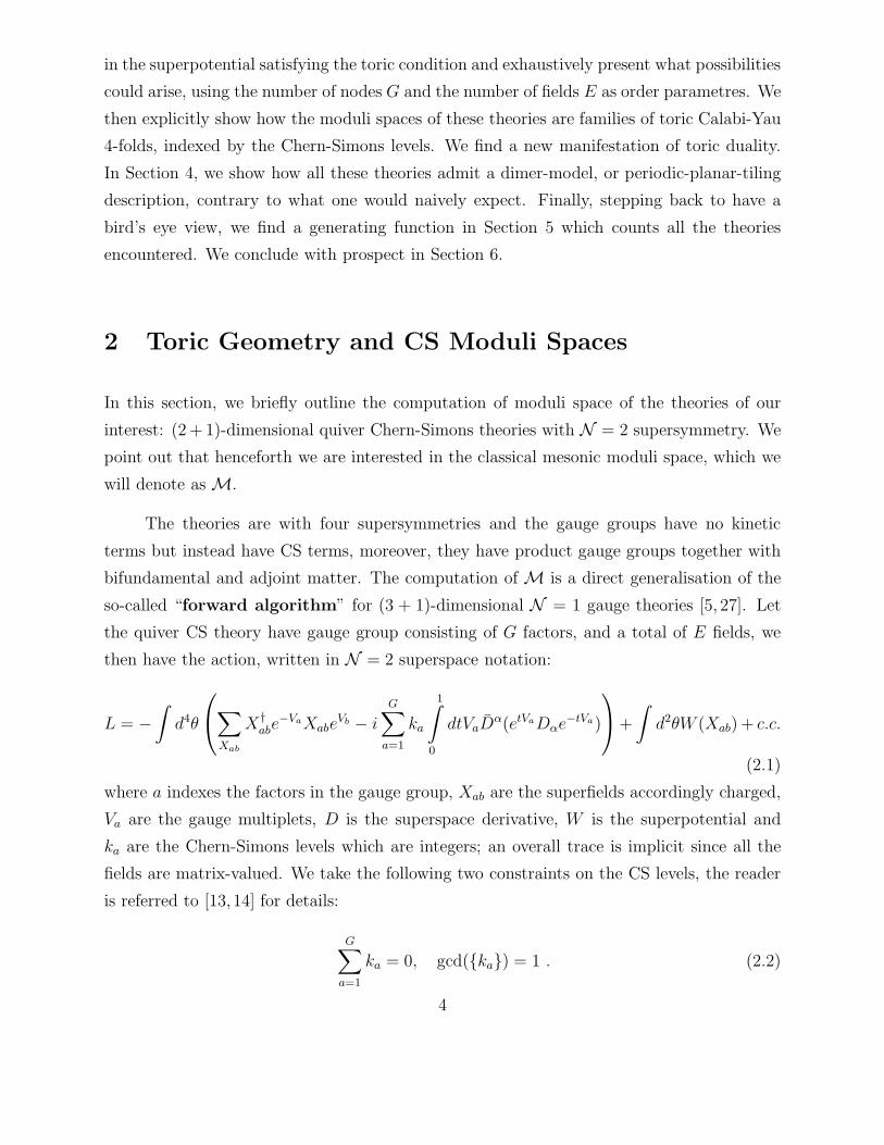
Contents

1 Introduction 2

2 Toric Geometry and CS Moduli Spaces 4

3 A Taxonomic Study 8

3.1 Four Fields in the Quiver . . . . . . . . . . . . . . . . . . . . . . . . . . . . . 10

3.2 Five Fields in the Quiver . . . . . . . . . . . . . . . . . . . . . . . . . . . . . 12

3.3 Six Fields in the Quiver . . . . . . . . . . . . . . . . . . . . . . . . . . . . . 13

3.4 Toric Diagrams: Illustrious Examples . . . . . . . . . . . . . . . . . . . . . . 15

3.5 A New Toric Duality . . . . . . . . . . . . . . . . . . . . . . . . . . . . . . . 18

4 Tilings: Dimers versus Crystals 19

5 A General Counting 20

5.1 A Systematic Enumeration . . . . . . . . . . . . . . . . . . . . . . . . . . . . 20

5.2 A Geometric Apercu . . . . . . . . . . . . . . . . . . . . . . . . . . . . . . . 23

6 Conclusions and Prospects 25

A Preliminary Classification 27

B Perfect Matchings from the Superpotential 27

1 Introduction

Recent advances in studying the world-volume theory of M2-branes [1, 2] have allowed new

perspectives on the AdS/CFT correspondence. Indeed, the three-dimensional theory on the

2

M2-branes is now understood as an ordinary gauge theory of Chern-Simons (CS) type [3,4].

The investigation of AdS4/CFT3 subsequently took flight, ever augmenting our arsenal of

dual pairs of theories.

One strand of development has been the extension of the elaborate structure of the

AdS5/CFT4 situation wherein the D3-brane world-volume gauge theory and the correspond-

ing Calabi-Yau cone over Sasaki-Einstein 5-folds have been probed in great detail over the

past decade. Of particular interest had been the cases where the Calabi-Yau threefold ad-

mits toric description. There, a rich tapestry, enabled by the abundant techniques of toric

geometry, had been woven over such themes as toric duality [5–7], dimer models and brane

tilings [9–11].

Along this vein, the parallel story for M2-branes probing toric Calabi-Yau 4-fold singu-

larities met with rapid progress [12–23], addressing such issues as tiling or its 3-dimensional

counter-part of crystal models, toric duality, as well as partition functions in the light of

the plethystic programme [24] etc. Thus inspired, especially by the fortitude to attack the

general singularity [15], it is expedient for us to take a synthetic approach. The space of toric

singularities of Calabi-Yau 4-folds is largely unchartered; nevertheless, we can gradually and

systematically list, starting from the simplest imaginable, the possible (2 + 1)-dimensional

quiver Chern-Simons theories. These theories are, of course, infinite in number; however,

we will see how the number of nodes in the quiver and the number of terms in the superpo-

tential can be used as order parametres to begin a classification. Even at low numbers, we

will encounter many highly non-trivial theories. Furthermore, we will establish generating

functions which counts the number of inequivalent theories at each level of our enumeration.

Remarkably, we can geometrically interpret these functions.

Thus, let us we embark on a journey through the complex terra incognita of new graphs

and associated superpotentials, guided by our experience with the techniques of (3 + 1)-

dimensional N = 1 gauge theory, mutatis mutandis, and slowly probe the dual pairs of toric

geometries and CS theories. A wealth of interesting properties will be encountered.

Our taxonomic study is organised as follows. We begin, in Section 2, with a brief

review of the computation of the moduli space of quiver Chern-Simons theories in (2 + 1)-

dimensions, culminating in an algorithmic flow-chart which generalises (and encompasses)

the “forward-algorithm” of [5] to the present case. Next, in Section 3, we begin our systematic

investigation of what toric Chern-Simons quiver theories can exist. We start with two terms

3

in the superpotential satisfying the toric condition and exhaustively present what possibilities

could arise, using the number of nodes G and the number of fields E as order parametres. We

then explicitly show how the moduli spaces of these theories are families of toric Calabi-Yau

4-folds, indexed by the Chern-Simons levels. We find a new manifestation of toric duality.

In Section 4, we show how all these theories admit a dimer-model, or periodic-planar-tiling

description, contrary to what one would naively expect. Finally, stepping back to have a

bird’s eye view, we find a generating function in Section 5 which counts all the theories

encountered. We conclude with prospect in Section 6.

2 Toric Geometry and CS Moduli Spaces

In this section, we briefly outline the computation of moduli space of the theories of our

interest: (2 + 1)-dimensional quiver Chern-Simons theories with N = 2 supersymmetry. We

point out that henceforth we are interested in the classical mesonic moduli space, which we

will denote as M.

The theories are with four supersymmetries and the gauge groups have no kinetic

terms but instead have CS terms, moreover, they have product gauge groups together with

bifundamental and adjoint matter. The computation of M is a direct generalisation of the

so-called “forward algorithm” for (3 + 1)-dimensional N = 1 gauge theories [5, 27]. Let

the quiver CS theory have gauge group consisting of G factors, and a total of E fields, we

then have the action, written in N = 2 superspace notation:

L = −

∫

d4θ

∑

Xab

X†abe

−VaXabeVb − i

G∑

a=1

ka

1∫

0

dtVaDα(etVaDαe−tVa)

+

∫

d2θW (Xab) + c.c.

(2.1)

where a indexes the factors in the gauge group, Xab are the superfields accordingly charged,

Va are the gauge multiplets, D is the superspace derivative, W is the superpotential and

ka are the Chern-Simons levels which are integers; an overall trace is implicit since all the

fields are matrix-valued. We take the following two constraints on the CS levels, the reader

is referred to [13, 14] for details:

G∑

a=1

ka = 0, gcd({ka}) = 1 . (2.2)

4

The classical mesonic moduli space M is determined by the following equations

∂XabW = 0

µa(X) :=G∑

b=1

XabX†ab −

G∑

c=1

X†caXca + [Xaa, X

†aa] = 4kaσa

σaXab − Xabσb = 0 , (2.3)

where σa is the scalar component of Va. Indeed, this is in analogy to the F-term and D-term

equations of N = 1 gauge theories in (3+1)-dimensions, with the last equation being a new

addition.

We are particularly interested in the case when M is a toric variety where the forward

algorithm conveniently uses the combinatorial power of lattice geometry and toric cones

[5, 25, 26]. This is the Abelian case where the gauge group is simply U(1)G. Physically,

M is a toric Calabi-Yau 4-fold transverse to an M2-brane on whose world-volume lives the

(2 + 1)-dimensional CS theory. For a stack of N parallel, coincident M-branes, the moduli

space is the N -th symmetrised product of (or more precisely the N -th Hilbert scheme of

points on) the 4-fold [4, 8, 13, 14].

In this Abelian, toric case then, the third equation of (2.3) sets all σa to a single field,

say σ, on the coherent component of the moduli space. The second equation causes the

D-terms to have FI-parametres 4kaσ. The moduli space M is a symplectic quotient of the

space of solutions to the F-terms prescribed by the first equation modulo the gauge conditions

prescribed by the D-terms. Because of the condition that all ka sum to 0 imposed in (2.2)

there is an overall U(1) (corresponding to the center of mass motion of the M2-brane) which

can be factored out. Furthermore, there is another U(1) which can be factored. This is

because the presence of CS couplings induces Fayet-Iliopoulos (FI) parameters on the space

of D-terms. In a generic (3 + 1)-dimensional theory all these FI parameters are arbitrary,

but here they are all aligned along a line which is parameterized by σ and has a direction

set by the CS integers. This picks out a very specific baryonic direction out of all possible

directions which are present in (3+1)-dimensions. This direction becomes mesonic in (2+1)-

dimensions and fibers over the Calabi-Yau 3-fold to give a total space as a Calabi-Yau 4-fold.

Thus, in all, there is a net of (G − 2) D-terms.

The space of solutions of the F-terms is itself a toric variety, of dimension 4+(G−2) =

G + 2, this is the so-called “Master space” F ♭G+2, studied in detail in [28]. Indeed, the

G − 2 D-terms are all the directions which remain baryonic in (2 + 1)-dimensions and give

5

rise to the Master Space1. Since we are interested in the mesonic moduli space, we impose

gauge invariance with respect to all of them. In summary,

M4 ≃ F ♭G+2//U(1)G−2 , (2.4)

where we have marked the complex dimensions explicitly as subscripts. The G − 2 FI-

parametres are shown in [14] to be in the integer kernel of the matrix

C =

(

1 1 1 . . . 1

k1 k2 k3 . . . kG

)

. (2.5)

To proceed we now recall the essential features in the computation of the 3+1 dimen-

sional mesonic moduli space of complex dimension 3. Computationally, the charges of the

fields are given by the so-called incidence matrix of the quiver; this is a G × E matrix.

Each column of this matrix representation of the quiver consists of two possible choices (1)

a single pair −1 and 1 denoting an arrow beginning and ending at the appropriate node and

zero elsewhere, or (2) an entire column of zeros, denoting an adjoint field charged only under

one single node.

The incidence matrix is customarily denoted as d and specifies the D-terms, i.e., the

U(1) toric actions. The crucial property of d is that each of its columns sums to 0 (since each

column corresponds to one arrow that necessarily has one head and one tail.) and that each

of its rows also sums to 0 (this ultimately ensures that the moduli space be Calabi-Yau2).

We emphasise the ambiguity for an adjoint: we do not know under which precise node it

is charged; from the point of view of the incidence matrix, there is no way to distinguish.

We will see later how using information from the superpotential one may overcome this

ambiguity.

Of course, one row of d is redundant because of the summation rule, we delete it and

customarily call the result ∆. On the other hand, the F-terms can be solved in terms of a

1There is a subtle point here. There are indeed G− 2 baryonic directions for a given Lagrangian with G

gauge groups. This does not imply that all possible baryonic directions of the particular CY4 are given by

these G − 2 directions. It only provides a lower bound. There are at least G − 2 such baryonic directions

and a different formulation may give more than this number. Such a situation is evident from the study of

models presented in [13–15].2Essentially, the reason is that one can translate the incidence matrix into the matrix of charges which

define the toric variety by right multiplication of a perfect matching matrix as shown in the ensuing flow-

chart. The Calabi-Yau condition, i.e., the vanishing of the first Chern class, is that the charges sum to zero

and subsequently requires that the rows of the incidence matrix also sum to zero [28].

6

matrix K, whose dual cone we call T . From these we can extract so-called U and V matrices.

We refer the reader to Section 2 of [5] for the details. Schematically we can summarise the

procedure of the “forward algorithm”, taken from cit. ibid., as follows:

Quiver → dG×E → ∆(G−1)×E

↓

F-Terms → KE×(G+2)V ·Kt=∆→ V(G−1)×(G+2)

↓ ↓

T(G+2)×c = Dual(K)U ·T t=Id→ U(G+2)×c → V U

↓ ↓

Q(c−G−2)×c = [Ker(T )]t −→ (Qt)(c−3)×c =

(

(V U)(G−1)×c

Q(c−G−2)×c

)

We have marked the dimensions of each matrix for clarity. Note that c is the number of

perfect matching in the dimer model [9] description of the theory to which we shall later

turn. The key point is that we can combine the matter content (specified by the incidence

matrix) and the superpotential (specified by the K-matrix) into a single charge matrix Qt;

its kernel, Gt, of dimension 3 × c, encodes the toric diagram of the Calabi-Yau threefold

moduli space. Refreshed with this recollection let us make one more step before getting back

to the main case of interest.

When dealing with 2+1 dimensional Chern-Simons theory the moduli space is a toric

4-fold. The above procedure should be modified to include the CS-levels by incorporating

the matrix C. First, let us recast the above flow-chart for a 3+1 dimensional theory in a

more succinct manifestation, dispensing of the need of the V and U matrices and introducing

the perfect-matching matrix PE×c = K · T and the trivial matrix (1, 1, 1, . . . , 1)1×G, which

by abuse of notation for now, we also call C:

INPUT 1:

Quiver→ dG×E → (QD)(G−1)×c = ker(C)(G−1)×G · QG×c , (dG×E := QG×c · (P T )c×E)

ր

INPUT 2:

Superpotential→ PE×c → (QF )(c−G−2)×c = [ker P ]t

↓

(Qt)(c−3)×c =

(

(QD)(G−1)×c

(QF )(c−G−2)×c

)

→OUTPUT:

(Gt)3×c = [Ker(Qt)]t

7

Note that we have judiciously called the charges coming from the D-terms QD and those

from the F-terms, QF . Moreover, we have even foregone the need for the matrix K, perhaps

so deeply engrained from our incipient days, and worked entirely in terms of the perfect-

matching matrix P ; there is indeed a conducive algorithm for extracting P directly from the

superpotential (cf. [15]). For the reader’s convenience, we summarise this in Appendix B.

Thus written, the generalisation to the case of present interest, viz. 2+1 dimensional

CS theories, is most straight-forward. We only need to modify the C matrix from the row of

ones to our current C2×G matrix defined in (2.5) which now includes the CS levels, thereby

changing the dimension of QD by 1, and subsequently causes Gt to have 4 rows:

INPUT 1:

Quiver→ dG×E → (QD)(G−2)×c = ker(C)(G−2)×G · QG×c ;

ր with dG×E := QG×c · (P T )c×EINPUT 2:

CS Levels→ C2×G

ր

INPUT 3:

Superpotential→ PE×c → (QF )(c−G−2)×c = [ker P ]t ;

↓

(Qt)(c−4)×c =

(

(QD)(G−2)×c

(QF )(c−G−2)×c

)

→OUTPUT:

(Gt)4×c = [Ker(Qt)]t

(2.6)

The matrix Gt represents the desired toric diagram: it should have columns of length 4,

signifying a 4-fold; moreover, these 4-vectors should be co-spatial, i.e., they all live in a

3-dimensional hypersurface, this is required by the Calabi-Yau condition. There could be

repetitions out of the c columns, this is the multiplicity, or perfect matchings, discussed

in [5, 7, 9, 29–32].

3 A Taxonomic Study

Having outlined the computational procedure, let us now proceed with a systematic study

of examples. Ideally, one would wish for a classification of all possible theories, their quiver

diagrams, interactions and subsequent geometries. This is a daunting task of organising

an infinite number of models. Nevertheless, we can proceed cautiously and modestly: let

8

us start with theories with a single pair of black-white nodes in the dimer picture. These

correspond to cases where the superpotential vanishes for a single brane; this is because the

so-called toric condition [6] requires that each field appears exactly twice with opposite

signs. In terms of the dimer model [9], this condition is what gives rise to the bi-partite

nature of the tiling. Of course, for multiple branes, because the fields become matrix-valued

and do not commute necessarily, the superpotential may no longer vanish. This is familiar

to us. For example, in the 3+1 dimensional gauge theory for the conifold 3-fold singularity

there is a quartic superpotential which vanishes for a single brane. We will encounter this

situation in detail below.

Hence, with a single M2 brane, and with only two terms therein, the superpotential

actually vanishes, subsequently, the master space is freely generated by the E fields and

is simply CE . Thus, the matter content completely specifies the 4-fold singularity. The

symplectic quotient (2.4) and the traditional approach both become relatively simple in this

case. In fact, in (2.6), c = E and the perfect matching matrix P is just the identity matrix.

The QF matrix for the F-terms are not present and we have that:

M ≃ CE//U(1)G−2 ∼ Gt = ker(ker(C)(G−2)×G · dG×E) , (3.1)

where ∼ means M has the toric diagram given by Gt of dimensions 4 × E.

Indeed, from (2.4), we see that E = G+2; let us hence use E as a single order parametre

and proceed gradually. We initiate with the case of two nodes, i.e., (G, E) = (2, 4). For each

incremental value of E, we classify all d-matrices satisfying the constraints which define the

incidence matrix. Indeed, in (3.1), ker(C)×d has dimensions (G−2)×(G+2) and its kernel

Gt will have columns of length 4, as is required for a toric diagram of a 4-fold.

In summary, our classification scheme for 2 terms in the superpotential proceeds as

follows:

1. Fix G, the number of nodes in the quiver. This also fixes the number of arrows as

E = G + 2;

2. Find all G × (G + 2) matrices which are incidence matrices, i.e., (a) each column is

one of only zeros (adjoint) or consists of a single pair of −1 and 1 and zero otherwise

(bi-fundamental), (b) each row sums to 0 (Calabi-Yau condition);

3. Identify all loops (gauge invariant operators) in the quiver drawn from each incidence

matrix and construct possible 2-term superpotentials satisfying (a) the toric condition,

9

i.e., each bi-fundamental field occurs exactly twice and with opposite sign and (b) for

a single brane when all the fields reduce from matrix-valued to complex numbers, the

2 terms conspire to cancel.

How do we attack step 2, the most computationally intense one? Luckily, the algorithms

for such a matrix-partitioning problem were implemented in [33] and we can thus happily

proceed with presenting the solutions. We adhere to the standard notation that

For bi-fundamentals X iab denotes the i-th arrow from node a to b and similarly

that φia denotes the i-th adjoint on node a (when there is only a single arrow the

i-index is dropped).

Already, there are many highly non-trivial theories.

3.1 Four Fields in the Quiver

Here, there are 2 nodes and we find only two non-isomorphic solutions. These are presented

in Figure 7 in the Appendix. There are two possibilities. In Model (1) we see that this is

a non-chiral theory with 4 bi-fundamentals. We recognise the quiver as that of the conifold

quiver. Indeed, the full superpotential for arbitrary N of that theory also has 2 terms:

calling the bi-fundamentals X i12 and X i

21, (i = 1, 2 and U(N) matrices) we have that W =

Tr(X112X

121X

212X

221 −X1

12X221X

212X

121), which indeed satisfies the toric condition and vanishes

for N = 1. The fact that we have CS constraints, of course, modifies the moduli space from

the 3-dimensional conifold to a CY 4-fold.

In Model (2), there are 2 adjoint fields and 2 bi-fundamentals. Where shall we place the

2 non-bi-fundamental fields in Model (2)? We can be guided by promoting to N > 1 number

of branes. There could be two possible placements: both as adjoints on 1 node or one on each

node. Calling the two bi-fundamentals X12 and X21, for both adjoints on the same node,

say node 2 without loss of generality, we have 2 gauge invariant terms: Tr(X12φ12φ

22X21) and

Tr(X12φ22φ

12X21). On the other hand, for one adjoint on each node we have only one possible

invariant: Tr(X12φ2X21φ1); this is because we need to be careful in matrix composition when

we go about the loops in the quiver to construct the gauge invariants. Therefore, Model (2)

has a natural candidate for a 2-term superpotential satisfying the toric condition and having

two terms, namely W = Tr(X12[φ12, φ

22]X21).

10

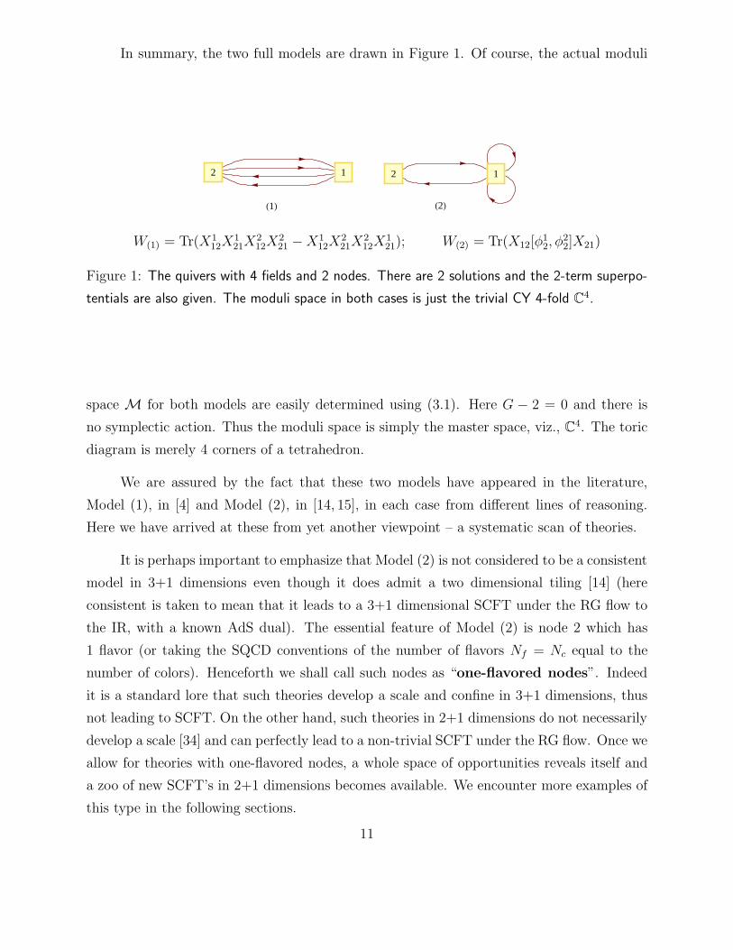
In summary, the two full models are drawn in Figure 1. Of course, the actual moduli

12 12

H1L H2L

W(1) = Tr(X112X

121X

212X

221 − X1

12X221X

212X

121); W(2) = Tr(X12[φ

12, φ

22]X21)

Figure 1: The quivers with 4 fields and 2 nodes. There are 2 solutions and the 2-term superpo-

tentials are also given. The moduli space in both cases is just the trivial CY 4-fold C4.

space M for both models are easily determined using (3.1). Here G − 2 = 0 and there is

no symplectic action. Thus the moduli space is simply the master space, viz., C4. The toric

diagram is merely 4 corners of a tetrahedron.

We are assured by the fact that these two models have appeared in the literature,

Model (1), in [4] and Model (2), in [14, 15], in each case from different lines of reasoning.

Here we have arrived at these from yet another viewpoint – a systematic scan of theories.

It is perhaps important to emphasize that Model (2) is not considered to be a consistent

model in 3+1 dimensions even though it does admit a two dimensional tiling [14] (here

consistent is taken to mean that it leads to a 3+1 dimensional SCFT under the RG flow to

the IR, with a known AdS dual). The essential feature of Model (2) is node 2 which has

1 flavor (or taking the SQCD conventions of the number of flavors Nf = Nc equal to the

number of colors). Henceforth we shall call such nodes as “one-flavored nodes”. Indeed

it is a standard lore that such theories develop a scale and confine in 3+1 dimensions, thus

not leading to SCFT. On the other hand, such theories in 2+1 dimensions do not necessarily

develop a scale [34] and can perfectly lead to a non-trivial SCFT under the RG flow. Once we

allow for theories with one-flavored nodes, a whole space of opportunities reveals itself and

a zoo of new SCFT’s in 2+1 dimensions becomes available. We encounter more examples of

this type in the following sections.

11

3.2 Five Fields in the Quiver

Here, there are 3 nodes and we find 5 distinct solutions. These are shown in Figure 8 in the

Appendix. Model (1) has 5 bi-fundamentals. Models (2) and (3) have 4 bi-fundamentals

and 1 adjoint field. Note that Model (2) has a disconnected node labelled 2. Model (4) has

3 bi-fundamentals and 2 adjoint fields and finally Model (5), also with a disconnected node,

has only 2 bi-fundamentals and 3 adjoint fields. Let us ignore models (2) and (4) since they

inevitably have reducible moduli spaces due to disconnected nodes.

For Model (1), using the standard notation, we clearly have the 2-term superpotential:

W = Tr(X21X113X31X

213X32 − X21X

213X31X

113X32), which satisfies the toric condition and

vanishes for N = 1 when all fields are simply complex numbers.

For Model (3), clearly there are two invariants X21X12 and X13X31. Where shall we

place the missing adjoint φ? It is easy to see that placing it on node 2 gives two invariants

once we promote to N > 1 branes, i.e., to matrix-valued fields: Tr(X21φ1X13X31X12) and

Tr(X21X13X31φ1X12). This indeed gives a two-term superpotential satisfying the toric con-

dition of each field appearing exactly twice with opposite signs: W = Tr(X21φ1X13X31X12 −

X21X13X31φ1X12); moreover, W indeed vanishes at N = 1 when all field are merely complex

numbers.

Finally, for Model (4), there are 2 ways of placing the 2 adjoints: both on the same node,

say node 1, or one each on 2 of the nodes. The latter possibility is ruled out since it would be

impossible to have 2 terms and satisfying the toric condition. However, putting both φi=1,21

on node 1, gives us a superpotential satisfying all requisites: W = Tr(X21[φ11, φ

21]X13X32).

We summarise all these good models in Figure 2.

It is important to note that none of these 3 models appeared previously in the literature.

Indeed, our systematic study revealed the existence of these 3 prototypical models. We will

proceed later by analyzing their properties and further introduce them from yet another

taxonomic viewpoint. It is further important to notice that all these models have a one-

flavored node and therefore do not correspond to consistent models in 3+1 dimensions even

though they all admit a brane tiling. Nevertheless they present a rich structure of non-trivial

SCFT’s in 2+1 dimensions with a highly intricate spectrum of scaling dimensions.

12

1

23

12 3

1

23

H1LH3L H4L

W(1) = Tr(X21X113X31X

213X32 − X21X

213X31X

113X32) ;

W(3) = Tr(X21φ1X13X31X12 − X21X13X31φ1X12) ;

W(4) = Tr(X21[φ11, φ

21]X13X32).

Figure 2: The quivers with 5 fields and 3 nodes. There are 3 good models and we call them (1),

(3) and (4). We also write the corresponding 2-term superpotentials.

3.3 Six Fields in the Quiver

Here, there are 4 nodes and there is a total of 18 distinct solutions. These are shown in

Figure 9 in the Appendix. Models (1) to (10) have 6 bi-fundamentals. Note that Models (1),

(2), (5) and (9) all have disconnected nodes. Model (8), though apparently acceptable, has

a superpotential in terms of its bi-fundamentals which looks like Tr(X31X14X42X24X41X13−

X42X24X41X13X31X14). This vanishes by cyclicity of the trace and hence it is really just a

theory without superpotential at all. Models (11) and (12) have 5 bi-fundamentals and 1

adjoint field. Models (13) to (16) have 4 bi-fundamentals and 2 adjoint fields. Note that

Models (13) and (14) both have disconnected nodes. Model (17) has 3 bi-fundamentals and

3 adjoint fields, as well as a disconnected node. Finally, Model (18) has 2 bi-fundamentals,

4 adjoint fields and 2 disconnected nodes. Once again, we select the diagrams without

detached nodes, insert the appropriate adjoint fields, and also write down the possible 2-

term superpotentials. We find a total of 6 possible models. These are presented in Figure 3.

Happily, we have again recovered and extended some of the known models in the

literature. Model (6) was proposed in Figure 3 of [15] for the Q1,1,1 geometry while Model

(10) was proposed in Figure 7 of [15] for the so-called D3 theory. The other models appear for

13

1

23

41

2 3

4 1

2

3

4

1

2 3

4

1

23

4

H4L H6L H7L

H10L H11L H16L

1

2

3

4

W(4) = Tr(X31X114X41X

214X42X23 − X31X

214X41X

114X42X23) ;

W(6) = Tr(X42X21(X114X43X31X

214 − X2

14X43X31X114)) ;

W(7) = Tr(X12X21(X14X41X13X31 − X13X31X14X41)) ;

W(10) = Tr(X42X21X14X41X13X34 − X42X21X13X34X41X14) ;

W(11) = Tr(X32X21φ1X14X41X13 − X32X21X14X41φ1X13) ;

W(16) = Tr(X42X23X31X14[φ14, φ

24])

Figure 3: The quivers with 6 fields and 4 nodes. There are 6 models. We also present the

superpotential as well as the adjoint-fields where necessary.

the first time in the literature. All models have a one-flavored node and so none correspond

to consistent models in 3+1 dimensions even though they all admit a brane tiling description.

For completeness we also include the two disconnected quivers, Models (3) and (15).

These engender multi-trace superpotentials because of the quivers factorise. We present

these in Figure 4. We see that they are essentially products of Models (1) and (2) of the

4-edged case, together with a 2-edged bi-fundamental non-chiral quiver. Also, we include

Model (8), which has a completely vanishing superpotential if it were to be 2-termed. We

will exclude these models from discussion in the following.

14

1

23

4

1

23

4

1 23 4

H3LH15L H8L

W(3) = Tr(X23X32) Tr(X114X

141X

214X

241 − X1

14X241X

214X

141)) ;

W(15) = Tr(X23X32) Tr(X14[φ14, φ

24]X41) ;

W(8) = Tr(X31X14X42X24X41X13 − X42X24X41X13X31X14) = 0 ;

Figure 4: The two disconnected quivers with 6 fields and 4 nodes, together with their multi-trace

superpotentials. Also Model (8) has completely vanishing superpotential.

3.4 Toric Diagrams: Illustrious Examples

Let us take, for concreteness, Model (1) of the E = 5 quivers, given in Figure 2. There are 3

nodes and hence 2 independent CS levels, k1 and k2. The toric diagram, according to (2.6),

is given by

G(1)t = ker(ker

(

1 1 1

k1 k2 −k1 − k2

)

·

(

−1 −1 0 1 1

0 0 1 −1 0

1 1 −1 0 −1

)

) = ker (−k2,−k2,−k1, k1 + k2, k2)

= gen

(

k2 0 0 0 k2

k1 + k2 0 0 k2 0

−k1 0 k2 0 0

−k2 k2 0 0 0

)

=

(

1 0 0 0 1

k1 + k2 0 0 k2 0

−k1 0 k2 0 0

−1 1 0 0 0

)

; gcd(k1, k2, k1 + k2) = 1 . (3.2)

In the penultimate step, we have been mindful of the fact we need to find the integer kernel

of the charge matrix and not merely the nullspace and hence we wrote gen( ) therein to

denote that we should reduce to a basis over the integers for whichever choice of k1 and

k2. This means that each row of Gt must have GCD being 1. Guaranteed by the condition

gcd(k1, k2,−k1 − k2) = 1, rows 2 and 3 are acceptable but rows 1 and 4 need to divide out

the common factor of k2; this gives the last step.

Indeed, each column of Gt is of length 4, signifying that the resulting moduli space

corresponding to this theory is a toric 4-fold. Furthermore, we see that the vector (1, 1, 1, 1)

is perpendicular to every pair-wise linear combination between the 5 column vectors, this

means that the columns are actually co-spatial, i.e., live on a dimension 3 hypersurface in

15

Z4; this, of course, guarantees that our 4-fold is in fact Calabi-Yau. Thus re-assured, we can,

without loss of generality, delete any row of Gt (call it G′t) and represent the toric 4-fold by

an integer polytope in 3-dimensions. Thus, we can write, for the toric diagram,

G′t = gen

(

1 0 0 0 1

−k1 0 k2 0 0

−1 1 0 0 0

)

, with gcd(k1, k2, k1 + k2) = 1 , (3.3)

where for convenience we have deleted the second row.

Now, depending on the choice of k1 and k2 obeying the coprimarity condition, we have

an infinite family of toric CY4s. As two illustrious examples we have that

G′t(k1 = 0, k2 = 1) =

(

1 0 0 0 1

0 0 1 0 0

−1 1 0 0 0

)

, G′t(k1 = 1, k2 = 1) =

(

1 0 0 0 1

−1 0 1 0 0

−1 1 0 0 0

)

(3.4)

We see that the two are not related by any SL(3; C) transformations and are thus inequivalent

toric varieties. We draw these diagrams explicitly in Figure 5.

1

(0,0,0)

(0,1,0)

(1,0,0)

(1,0,−1)

(0,0,1)

(0,0,0)

(0,1,0)

(0,0,1)

(1,−1,−1)

(1,0,−1)

(a) (b)

Figure 5: The two moduli spaces, drawn with explicit toric diagrams, for different choices of

Chern-Simons levels (a) (k1, k2) = (0, 1) and (b) (k1, k2) = (1, 1) for Model (1) of the 5-edge,

3-noded theory with 2-term superpotential.

The other two models of the E = 5 quiver theories can be similarly treated. For Model

(3), we have that

G(3)t = ker(ker

(

1 1 1

k1 k2 −k1 − k2

)

·

(

−1 −1 1 1 0

0 1 −1 0 0

1 0 0 −1 0

)

) = ker({−k2, −k1 − k2, k1 + k2, k2, 0})

= gen

(

0 0 0 0 k2

k2 0 0 k2 0

k1 + k2 0 k2 0 0

−k1 − k2 k2 0 0 0

)

=

(

0 0 0 0 1

1 0 0 1 0

k1 + k2 0 k2 0 0

−k1 − k2 k2 0 0 0

)

; gcd(k1, k2, k1 + k2) = 1 . (3.5)

16

This, as above, gives an infinite family, parametrised by choices of k1 and k2, of possibilities

for the moduli space M and hence inequivalent theories.

Finally, for Model (4), we have

G(4)t = ker(ker

(

1 1 1

k1 k2 −k1 − k2

)

·

(

−1 0 1 0 0

0 1 −1 0 0

1 −1 0 0 0

)

) = ker({−k2, −k1, k1 + k2, 0, 0})

= gen

(

0 0 0 0 k2

0 0 0 k2 0

k1 + k2 0 k2 0 0

−k1 k2 0 0 0

)

=

(

0 0 0 0 1

0 0 0 1 0

k1 + k2 0 k2 0 0

−k1 k2 0 0 0

)

; gcd(k1, k2, k1 + k2) = 1 . (3.6)

An Interesting Family: Examining Model (1) of Figure 2 and Model (4) of Figure 3,

it is clear that for the general case of G nodes and E = G + 2 fields, there will always be

a cyclically-directed G-gon graph with 1 edge having an extra pair of arrows in opposite

directions. Thus all E fields are bi-fundamentals and let us, without loss of generality, place

the extra pair of bi-fundamentals between nodes 1 and G, and let the direction of the arrows

be 1 → 2, 2 → 3, . . . , (G − 1) → G and G → 1. The quiver and adjacency matrices are

3

1

G

2

d =

−1 0 . . . 1 1 −1

1 −1 . . . 0 0 0

0 1 . . . 0 0 0... 0

......

......

0 0 . . . −1 −1 1

G×(G+2)

(3.7)

The 2-term superpotential is also straight-forward to write down:

W = Tr(

X12X23 . . .XG−2,G−1(X1G−1,1X1,G−1X

2G−1,1 − X2

G−1,1X1,G−1X1G−1,1)

)

. (3.8)

We can also apply (2.6) to the incidence matrix to find the toric diagram. The result

has E = G + 2 lattice points:

Gt =

1 0 −k3 −(k3 + k4) . . . −(k3 + . . . + kG−1) 0 0 −k1 − k2

0 1 k2 + k3 k2 + k3 + k4 . . . k2 + . . . + kG−1 0 0 k1

0 0 0 0 . . . 0 1 0 1

0 0 0 0 . . . 0 0 1 1

4×(G+2)

(3.9)

17

Six Field Models: For completeness, let us present the matrices Gt encoding the toric

diagrams for the 6 models at E = 6, drawn in Figure 3. They are, respectively,

G(4)t =

(

1 0 0 0 0 1

k1 + k2 + k3 0 k2 0 k2 + k3 0

−k1 0 k3 k2 + k3 0 0

−1 1 0 0 0 0

)

, G(6)t =

(

k1 + k2 0 −k3 0 0 k2

1 0 1 0 1 0

−k1 0 k3 k2 0 0

−1 1 0 0 0 0

)

G(7)t =

(

0 1 0 0 0 1

1 0 0 0 1 0

k1 + k2 + k3 −k3 0 k2 0 0

−k1 − k2 − k3 k3 k2 0 0 0

)

, G(10)t =

(

1 0 0 0 0 1

k1 + k2 + k3 −k3 0 0 k2 0

−k1 − k3 k3 0 k2 0 0

−1 1 1 0 0 0

)

G(11)t =

(

0 0 0 0 0 1

1 0 0 0 1 0

1 0 1 1 0 0

−1 1 0 0 0 0

)

, G(16)t =

(

0 0 0 0 0 1

0 0 0 0 1 0

k1 + k2 + k3 k2 0 k2 + k3 0 0

−k1 k3 k2 + k3 0 0 0

)

(3.10)

3.5 A New Toric Duality

In its original guise, toric duality [5] referred to the phenomenon of 4-dimensional, N = 1

gauge theories having the same vacuum moduli space as toric varieties, some classes of these

were later realised to be Seiberg dualities. In our host of examples above, we have again

encountered this duality, now in a more general setting.

Take the two models of E = 4, they, even though having quite different quivers, share

the same infrared moduli space as C4. Perhaps more dramatic is the following pair: take

Model (4) of E = 5 at (k1, k2) = (1, 1) and inspect (3.6), then take Model (16) of E = 6 at

(k1, k2, k3) = (1, 0, 1) and inspect (3.10), we see that they are

GE=5, Model(4)t =

(

0 0 0 0 1

0 0 0 1 0

2 0 1 0 0

−1 1 0 0 0

)

, GE=6, Model(16)t =

(

0 0 0 0 0 1

0 0 0 0 1 0

2 0 0 1 0 0

−1 1 1 0 0 0

)

. (3.11)

We see that if we removed a repeated column in the latter, which does not influence the

toric description, the moduli spaces of the two theories, which have different number of

gauge group factors, different matter content and interactions and different Chern-Simons

levels, are identical as toric varieties. Clearly there are infinitely many such cases and it is

interesting to study the systematics of this phenomenon.

18

4 Tilings: Dimers versus Crystals

It is now well-established that the most convenient and elegant way of encoding the (3 + 1)-

dimensional quiver gauge theory of D3-branes probing toric Calabi-Yau threefold singularities

is through the formalism of dimer models, or, equivalently, brane-tilings [9–11]. The afore-

mentioned “toric condition” [6] of the superpotential is naturally interpreted as the bi-partite

(2-colour) property of the tiling while the Calabi-Yau condition of the threefold, which

compels the toric diagram to be planar, gives the inherent structure of periodic tiling of

the 2-dimensional plane. One question which has emerged is how this would generalise to

toric varieties of higher dimension. Indeed, proposals have been made which suggest that a

3-dimensional analogue of the dimer, a so-named “crystal model”, should encode the toric

Calabi-Yau 4-fold case [15, 19, 21]. Is this so for the 4-folds we have encountered in our

investigation?

Surprisingly, we find all our above CS theories to afford 2-dimensional tilings, rather

than the naively expected crystals which tile 3-dimensions. Let us recall that for the (3+1)-

dimensional gauge theories, an important relation exists [10]:

NT − E + G = 0 , (4.1)

where NT is the number of terms in the superpotential, while E and G, as above, are the

number of fields and gauge group factors. The recognition of (4.1) as the topological Euler

equation for the simplex decomposition of a genus 1 Riemann surface Σ, with a number NT

of vertices, a number E of edges and a number G of faces was key to the birth of the dimer

model. Indeed, the graph dual of this simplex is a periodic version of writing the quiver

diagram together with the superpotential, the periodicity further supporting the existence

of Σ as a torus.

How does this crucial relation read for our (2+1)-dimensional CS theories? Here, since

we are only considering 2-term superpotentials, NT = 2. Moreover, recall that E = G + 2

from (2.4). Therefore 2 − (G + 2) − G = 0 and (4.1) is still satisfied! This is not what one

would expect from a crystal model which is not a periodic tiling of the plane but which is

perhaps at first expected for all toric 4-fold theories. In summary, we have that

All quiver Chern-Simons theories corresponding to a M2-brane probing a toric

Calabi-Yau 4-fold, such that the superpotential has two terms, admit a dimer

model (2d-tiling) description.

19

5 A General Counting

We could have continued the process of Section 3 ad infinitum, listing more and more graphs

and then for each, construct possible superpotentials with 2 terms or fix various values of

Chern-Simons levels to obtain infinite families of toric moduli spaces. This, though explicit,

is perhaps not so illustrative, let alone computationally prohibitive. It would, however, be

most enlightening if we could count, say, the number of possible quivers for a given number

of nodes. In this section, let us give a generating function to perform this count; we will find

an elegant result very much in the spirit of the Plethystic Programme [24].

5.1 A Systematic Enumeration

To this end, we shall introduce a systematic enumeration and construction of the quivers.

Let us do so by the concept of base node which we now introduce. Examining Model (2) of

Figure 1, Models (3) and (4) of Figure 2, as well as Models (7), (11) and (16) of Figure 3,

we see that they, perhaps not immediately obviously, fall into a family. These are all models

which have a single base node, viz., a single reference node whence loops depart and thence

return. Let us consider a chain of closed paths beginning and ending on this same node (cor-

responding to a possibly multi-trace gauge invariant operator) and denote it by a sequence

of non-negative integers each entry of which encodes the length of one loop. Clearly, this

sequence is unordered. For example, for the simple quiver which has a single node with 3

self-loops attached (incidentally, this is the quiver of the N = 4 super-Yang-Mills theory for

D3-branes in flat C3 paradigmatic in the first AdS/CFT pair), we would denote it as 000,

drawn in Figure 6.

1

Figure 6: The quiver for N = 4 Super-Yang-Mills, corresponding to a D3-brane in flat C3. This

is a single-noded, triple-edged quiver, which we denote as 000.

20

Next, what would 001 (and of course any of its permutations) denote? This is Model

(2) of Figure 1, which has 2 loops of length 0 and 1 loop of length 1. Note that by length

here we mean the number of different nodes traversed before returning. Similarly, 011 and

002 correspond to Models (3) and (4) of Figure 2 respectively. Likewise, we retrieve the 3

aforementioned models for E = 6 fields corresponding to 111, 012 and 003. The systematics

is thus clear. For E fields and G = E − 2 nodes, we are counting graphs which are in

correspondence with unordered partitioning of G − 1 into 3 parts of non-negative integers.

This is a standard problem, whose solution is simply

f1(t) =1

(1 − t)(1 − t2)(1 − t3)= 1 + t + 2t2 + 3t3 + . . . (5.1)

This function was indeed encountered in [24] as the generating function for 1 adjoint field

with N = 3 D3 branes. The above is the generating function such that the coefficient in

front of tG−1=E−3 gives the number of quivers of 1 base node with G nodes. These are all

quivers with 3 primitive loops.

Having addressed one family of quivers transcending across E, the family with a single

base node, let us move onto 2 base nodes, say 1 and 2. Now, it is more convenient to count

by open paths: we let n1n2m1m2 denote a configuration which has open paths of length n1,

m2, m1, n2 respectively starting at node 1, ending at node 2, starting at node 2 and ending

at node 1. Again, by length we mean distance away from the base pair. These are all quivers

with 4 primitive paths between the 2 base nodes. Specifically, 0000 would correspond to

Model (1) of Figure 1. Next, taking the base pair to be nodes 3 and 1, 0001 would denote

Model (1) of Figure 2. Moving on to 4 nodes and 6 fields, we see that 0002, 0011 and 0101

denote respectively Models (4), (6) and (10) of Figure 3 when taking nodes 4 and 1 and

the base pair. This is analogous to the above, but is the unordered partitioning of G − 2

into 4 non-negative integers with the extra complication that we must respect the di-hedral

symmetry. Specifically, the transpositions (n1 ↔ n2), (m1 ↔ m2), (n1n2 ↔ m1m2) generate

a dihedral group of order 8. Orbits under these 8 elements must be quotiented out. The

generating function for this also admits a standard solution by method of Molien series [24]

for the dihedral group, in a 4-dimensional representation acting on our 4-vector:

f2(t) =1 − t6

(1 − t)(1 − t2)2(1 − t3)(1 − t4)= 1 + t + 3t2 + 4t3 + 8t4 + . . . (5.2)

Here, the coefficient of tG−2 is the number of models with G = E − 2 nodes.

What about triplets or more of base nodes? Note that our above two have already

exhausted all the quivers we have so far explicitly constructed. Could there be more families

21

which one might encounter at higher E? We now argue that we shall, in fact, not. First, let us

recall that our counting procedure above of course does not include any disconnected graphs

and moreover excludes shapes such as Model (8) of Figure 4. This is a 3-base-node example;

however, we have explicitly shown that the superpotential vanished. Indeed, the cases of

base nodes being one or two precisely permitted us to write a commutation relation allowing

for the two terms in the superpotential: the case of the 1-base-node achieved with the adjoint

and the case of the 2-base-node, with the pair of bi-fundamentals between them. Any other

case must either be reducible to these two situations or have vanishing superpotential.

Indeed, we can use an additional symmetry to restrict the possible models. Consider

the number of flavours niE for a given node i: this is either an incoming-outgoing pair of

arrows or an adjoint. The vector niE for i = 1, . . . , G is an additional order parameter. From

our examples, we see that it is 1 for most nodes. This is the one-flavoured node we discussed

earlier. However, it must be at least 1 for every node since we are not counting disconnected

quivers and it must never exceed 3 since there are only E = G+2 number of arrows in total.

Clearly, the sum of niE over i is equal to E = G + 2. Therefore, there are only 2 possibilities

for the components of the vector: (a) G − 1 of them being 1 and a single 3 or (b) G − 2 of

them being 1 and 2 of them being 2.

Subsequently, this places a significant restriction on the total number of adjoints. Since

each node must have at least one bi-fundamental, case (a) could have up to 2 adjoints on

the last node and case (b) could have up to a single adjoint on the last two nodes. Hence,

in total there could really only be 0, 1 or 2 adjoints. Now, we see that any node which

has no adjoint and only an incoming/outgoing pair of arrows is a descendent of a simpler

configuration: namely replace this node, together with its 2 attached arrows, with a single

arrow between the 2 nodes from which the said node emanates. Therefore, we need only

consider the parent quivers of (a) and (b), viz., a single node with flavour number 3 or two

nodes each with flavour number 2, respectively. The former is 000. The latter has two

possibilities: 0000 and a quiver which looks like12

; we can easily show that

the latter admits no non-vanishing 2-term superpotential. Indeed, Model (8) of Figure 4

discussed above is a descendent thereof and also needs to be eliminated.

In summary, we only need to consider descendents of the 3-vector 000 and the 4-vector

0000 and no quivers with more than 2 base nodes survive. Hence, f1 and f2 together exhaust

all counting. Furthermore, noticing the shift in power of f2 with respect to f1, we conclude

that:

22

The number of theories of our interest, i.e., all non-trivial, connected models with

2 terms in a non-vanishing superpotential and G = E − 2 nodes, is counted by

the coefficient of tG−1 in the expansion of the generating function

f(t) = f1(t) + tf2(t) =1 + t + t3 − t4 + t5

(1 − t)(1 − t2)(1 − t3)(1 − t4). (5.3)

5.2 A Geometric Apercu

The forms of f1 and f2 are perhaps familiar to the astute reader. The first, is the Hilbert

series (cf. [24]) for the weighted projective plane WP2[1:2:3] (or, alternatively the quotient

C3/S3 of the symmetric group on 3 objects), and the second, that of the 4-fold quotient

singularity C4/D4, i.e., the orbifold of C4 by the dihedral group of order 8 (cf. [35] for

discrete subgroups of SU(4)). It is quite elegant that these two geometrical spaces should

encode the entire space of quivers of our type.

In fact, quivers of the first family, the single-base-node type, obey a simple rule of

composition, reflecting the fact that there is an underlying commutative algebra which is

freely generated: the zero element is the self-adjoining loop, 1 is the quiver with 2 nodes and

a pair of bi-fundamentals in opposite directions between them, and thus generalising to n,

which is the quiver that is an n-gon with bi-fundamentals cyclically going around once. We

can create a quiver by selecting any 3 from this list and composition is by pasting the three

at a chosen common node:

Composition e.g. 0 + 1

>

> > >

> >

>

> >

...

0 1 n

In terms of the 3-vector of integers, we can also see this composition. For example, 001 +

23

011 = 012 refers to the following pasting of quivers

012

>

>

>>>

>

>

>

>>

>

>

>

>

>

=+

001 011

Indeed, we have drawn the result in a suggestive form, so as to indicate that such a compo-

sition corresponds to the insertion of nodes. Specifically, adding n1n2n3 signifies inserting,

after choosing an absolute ordering of the loops, n1, n2 and n3 nodes into the loops. In

this fashion, we readily see that the quivers 001, 011 and 111 generate, by this insertion

procedure, all quivers with one base node. Thus, we have an algebra freely generated by the

three elements:

12 1 2 3

1

2

3

4

001 011 111

The second family is a little more involved. We can define the 0 element as a node

with an out-going arrow, 1 as a node with an incoming and an out-going arrow, etc.:

>> >>

0 1 n

... >

>

Composition is by again pasting, though this time we must first paste to create a pair of

base nodes, unto which we may then attach the open arrows of the element n. Finally, we

24

must eliminate the redundancies of quivers which obey dihedral symmetry. In terms of the

4-vector, we now have an algebra generated by 5 elements, 0001, 0011, 0101, 0111 and 1111:

1

23

1

2 3

4

1

2 3

41

2

3

4

51

2

3

4

5

6

0001 0011 0101 0111 1111

obeying a single relation.

We have thus uncovered an algebraic structure on the space of CS quivers with 2-

term superpotentials. This is expected to persist to higher number of terms and indeed to

the space of all quivers; we have thus found an underlying algebraic variety for the set of

Chern-Simons quivers. We remark also that taking the plethystic logarithm [24] of the total

f(t) reveals that it is a non-terminating series suggesting that the algebraic variety is not a

complete intersection. It is in the form of a set union of the two orbifolds, though there is a

degree shift on the second.

6 Conclusions and Prospects

In this paper we have started a taxonomic study of quiver Chern-Simons theories in (2+ 1)-

dimensions. In particular, we study the theories arising from M2-branes probing toric Calabi-

Yau 4-fold singularities. Our purpose is not to merely provide a catalogue of such theories

since there are clearly infinite families thereof, but to study the space of these theories from

both a synthetic and an analytic approach, and to uncover interesting physical phenomena

as well as mathematical structure. Some of the techniques and concepts can indeed be

generalised to quiver theories in arbitrary dimension and with any supersymmetry.

We have first presented, in flow-chart (2.6), a succinct way of a “forward algorithm”

which takes the quiver and superpotential data as input and the moduli space as an output:

the former as a pair of matrices, respectively the incidence and the perfect matching matrices,

and the latter, as a matrix representing the integer coordinates of the toric diagram of

the Calabi-Yau 4-fold. The intermediate computations involve nothing more than matrix

multiplications and finding kernels. Indeed, this generalises and significantly improves on

25

the forward-algorithm of the case of (3 + 1)-dimensional gauge theories of [5]: we only need

to insert a C-matrix of the Chern-Simons levels and have obviated the need for finding dual

cones.

Thus armed, we have commenced the classification of all quiver Chern-Simons theo-

ries. Listing the quivers is matter of combinatorics and for simplicity we have taken the

superpotential to have two terms. It is clearly a pressing problem what happens at an ar-

bitrary number NT of terms, this we shall leave to forth-coming work. Subsequently our

order parametre becomes G, the number of nodes and E, the number of arrows, is equal

to G + 2 since the master space here is CE . In general, we should have 3 order parametres

(E, G, NT ). We exhaustively list the first members at E = 4, 5, 6 and find many non-trivial

theories, including and extending beyond what has so far emerged in the literature.

Because of our forward algorithm, we can readily determine the toric Calabi-Yau 4-

fold moduli spaces for all the theories presented. These exhibit as many toric varieties, each

of which is an infinite family, indexed by the integer Chern-Simons levels. Remarkably we

have once more encountered the phenomenon of “toric duality” first noted in [5] for (3 + 1)-

dimensional gauge theories. Now, it has manifested in perhaps some more striking guises: we

find not only theories with the same number of nodes but also those with different number

of nodes, fields, as well as Chern-Simons levels, to flow to the same IR moduli space as toric

Calabi-Yau 4-folds. It is certainly of importance to study what is precisely happening in the

field theory of such pairs.

Building upon our host of examples, we have stepped back for a panoramic view of all

our theories: connected quiver Chern-Simons with 2-term toric superpotentials. Though the

graphs seem unwieldy and growth rapidly in number as we increase the number of nodes,

we have found a generating function (5.3) which counts the number of inequivalent theories

given the number of nodes. Remarkably, this generating function splits conveniently into

2 pieces, each of which is the Hilbert series of a precise algebraic variety: the non-Abelian

quotient space C3/S3 by the symmetric group on 3 objects of order 6 and the Abelian

quotient C4/D4 by the ordinary dihedral group of order 8 (i.e., the symmetry group of the

square). Could we package the case with arbitrary (E, G, NT ) into a convenient tri-variate

generating function and would the result have an interpretation as a Hilbert Series, whereby

suggesting that the space of quiver theories is itself some algebraic variety? In answering

this and many questions raised we are presently engaged. Indeed, we have only tread upon

the fringe of a vast and fertile land, into her bountiful bosom we must onwardly march.

26

Acknowledgments

Scientiae et Technologiae Concilio Y.-H. H. hoc opusculum dedicat cum gratia ob honorem

officiumque Socii Progressi collatum. Et Ricardo Fitzjames, Episcopo Londiniensis, ceter-

isque omnibus benefactoribus Collegii Mertonensis Oxoniensis quorum beneficiis pie, stu-

diose, iucunde vivere licet, pro amore Catharinae Sanctae Alexandriae et ad Maiorem Dei

Gloriam.

A Preliminary Classification

In this appendix, we present the results for a preliminary classification of the case of 2 terms

in the superpotential. This will include cases of disjoint quivers and unmarked adjoint fields,

we present them here for completeness. The cases of 4, 5 and 6 fields are respectively shown

in Figures 7, 8 and 9. In the text we will sift through these graphs carefully, adding adjoints

wherever consistent.

12 12

H1L H2L

Figure 7: The quivers with 4 fields and 2 nodes. There are 2 solutions. Note that Model (2) has

only 2 arrows because it has 2 adjoint fields which are not drawn.

B Perfect Matchings from the Superpotential

In this appendix, we extract the matrix P of perfect matchings directly from the superpoten-

tial W ({Xi}) of the fields Xi=1,...,E. In the archaic days of the forward algorithm, P is found

27

1

23

1

2

312 3

1

23

1

2

3

H1L H2L H3L

H4L H5L

Figure 8: The quivers with 5 fields and 3 nodes. There are 5 solutions. Note that all quivers

with explicitly less than 5 arrows have adjoint fields which are not drawn.

to be the product of the matrix K (which encodes how a total of E F-terms can be solved

in terms of a fewer number) with its dual cone matrix T . Now we can follow the ensuing

prescription to directly obtain P without the rather computationally intensive procedure of

finding dual cones:

1. Group all the monomials appearing in W into those with positive coefficients and those

with negative, giving us two sets of equal length (since each field must appear exactly

twice with opposite signs by the toric condition), on each of which we choose an order;

2. Find the position of field X in each of the two sets; say it is i-th in the positive set

and j-th in the negative set. Construct a matrix whose (i, j)-th entry is X (should the

index ever repeat, simply add, to the entry, the new field). Do so for all E fields and

patch in zeros otherwise. This is the Kasteleyn matrix. Compute its determinant D.

3. D is a new polynomial in the E fields with c (the number of perfect matchings) terms.

Fix an order for these terms, and construct and E × c matrix. For each of the E fields

find the location in the monomial in D. We place a 1 at this location in the E-th row

28

123

4 123 4

1

23

4

1

23

41

2

34 1

2 3

41

2

3

4

1 23 4

1

2

34 1

2 3

4

1

2

34

1

2

3

4

123

4

123 4

1

23

4

1

23

4

1

2

34

123

4

H1L H2L H3L

H4L

H5L H6L H7L H8L

H9L H10LH11L

H12L

H13L

H14L

H15L

H16L

H17L H18L

Figure 9: The quivers with 6 fields and 4 nodes. There are 18 solutions. Note that all quivers

with explicitly less than 6 arrows have adjoint fields which are not drawn.

correspondingly and 0 otherwise. The resulting matrix is the desired P .

29

As an illustrative example, let is consider the famous cone over the zeroth del Pezzo

surface, i.e., the Abelian orbifold C3/Z3. Its quiver is a directed loop over 3 nodes, each with

multiplicity 3 and its superpotential is a six term cubic in 9 fields:

W =3∑

i,j,1

ǫijkXi1,2X

j2,3X

k3,1 . (B.1)

We recall that (cf. e.g., Eq. (2.12) - (2.17) of [28]) the explicit solutions to the F-terms are

X11,2 =

X31,2 X1

3,1

X33,1

, X21,2 =

X31,2 X2

3,1

X33,1

, X12,3 =

X32,3 X1

3,1

X33,1

, X22,3 =

X32,3 X2

3,1

X33,1

and hence

K =

X11,2 X2

1,2 X31,2 X1

2,3 X22,3 X3

2,3 X13,1 X2

3,1 X33,1

X31,2 1 1 1 0 0 0 0 0 0

X32,3 0 0 0 1 1 1 0 0 0

X13,1 1 0 0 1 0 0 1 0 0

X23,1 0 1 0 0 1 0 0 1 0

X33,1 −1 −1 0 −1 −1 0 0 0 1

, T = Dual(K) =

0 0 1 1 0 0

0 0 1 0 1 0

1 0 0 0 0 1

0 1 0 0 0 1

0 0 1 0 0 1

,

(B.2)

where Dual refers to finding the dual cone. The product Kt · T is the matrix P .

Using our new algorithm, we find that there are 3 positive terms and 3 negative terms,

giving us a Kasteleyn matrix and its determinant D as:

Kas =

(

X13,1 X3

2,3 X21,2

X31,2 X2

3,1 X12,3

X22,3 X1

1,2 X33,1

)

,D = X1

1,2X21,2X

31,2 − X3

2,3X33,1X

31,2 + X1

2,3X22,3X

32,3

−a(1)X12,3X

13,1 − X2

1,2X22,3X

23,1 + X1

3,1X23,1X

33,1

(B.3)

Upon comparison, we find that both procedures give (up to trivial permutation of columns,

note that we have fixed the row by a canonical ordering of the fields) P =

0

B

B

B

B

B

B

B

B

B

B

B

B

B

B

B

B

@

1 0 1 0 0 0

1 0 0 1 0 0

1 0 0 0 1 0

0 1 1 0 0 0

0 1 0 1 0 0

0 1 0 0 1 0

0 0 1 0 0 1

0 0 0 1 0 1

0 0 0 0 1 1

1

C

C

C

C

C

C

C

C

C

C

C

C

C

C

C

C

A

.

We must point out that on a simple timing contrast, our new algorithm for this simple

example is about a factor of 10 faster! This is significant since the algorithm for finding dual

cones is exponential running time so for bigger examples, we expect that our new method to

be a substantial improvement. For example, for the cone over the third del Pezzo surface,

with 14 fields and 8 terms in the superpotential, our present algorithm constitutes a time

reduction of more than 1000-fold over the old dual-cone method! It would be interesting to

see whether this technique could be generalised to rapidly find the dual cone of arbitrary

integer cones; this would of tremendous use to toric geometry.

30

References

[1] J. Bagger and N. Lambert, “Modeling multiple M2’s,” Phys. Rev. D 75, 045020

(2007) [arXiv:hep-th/0611108]. “Gauge Symmetry and Supersymmetry of Multiple M2-

Branes,” Phys. Rev. D 77, 065008 (2008) [arXiv:0711.0955 [hep-th]]. “Comments On

Multiple M2-branes,” JHEP 0802, 105 (2008) [arXiv:0712.3738 [hep-th]].

[2] A. Gustavsson, “Algebraic structures on parallel M2-branes,” arXiv:0709.1260 [hep-

th]. “Selfdual strings and loop space Nahm equations,” JHEP 0804, 083 (2008)

[arXiv:0802.3456 [hep-th]].

[3] M. Van Raamsdonk, “Comments on the Bagger-Lambert theory and multiple M2-

branes,” JHEP 0805, 105 (2008) [arXiv:0803.3803 [hep-th]].

[4] O. Aharony, O. Bergman, D. L. Jafferis and J. Maldacena, “N=6 superconformal Chern-

Simons-matter theories, M2-branes and their gravity duals,” arXiv:0806.1218 [hep-th].

[5] B. Feng, A. Hanany and Y. H. He, “D-brane gauge theories from toric singularities and

toric duality,” Nucl. Phys. B 595, 165 (2001) [arXiv:hep-th/0003085].

[6] B. Feng, S. Franco, A. Hanany and Y. H. He, “Symmetries of toric duality,” JHEP

0212, 076 (2002) [arXiv:hep-th/0205144].

[7] B. Feng, A. Hanany and Y. H. He, “Phase structure of D-brane gauge theories and toric

duality,” JHEP 0108, 040 (2001) [arXiv:hep-th/0104259].

[8] D. Berenstein, “Reverse geometric engineering of singularities,” JHEP 0204, 052 (2002)

[arXiv:hep-th/0201093].

[9] A. Hanany and K. D. Kennaway, “Dimer models and toric diagrams,” hep-th/0503149.

[10] S. Franco, A. Hanany, K. D. Kennaway, D. Vegh and B. Wecht, “Brane dimers and

quiver gauge theories,” JHEP 0601, 096 (2006) [arXiv:hep-th/0504110].

[11] B. Feng, Y. H. He, K. D. Kennaway and C. Vafa, “Dimer models from mirror symmetry

and quivering amoebae,” Adv. Theor. Math. Phys. 12, 3 (2008) [arXiv:hep-th/0511287].

[12] N. Lambert and D. Tong, “Membranes on an Orbifold,” Phys. Rev. Lett. 101, 041602

(2008) [arXiv:0804.1114 [hep-th]].

31

[13] A. Hanany and A. Zaffaroni, “Tilings, Chern-Simons Theories and M2 Branes,”

arXiv:0808.1244 [hep-th].

[14] A. Hanany, D. Vegh, A. Zaffaroni, “Brane Tilings and M2 Branes,” arXiv:0809.1440.

[15] S. Franco, A. Hanany, J. Park and D. Rodriguez-Gomez, “Towards M2-brane Theories

for Generic Toric Singularities,” arXiv:0809.3237 [hep-th].

[16] M. Benna, I. Klebanov, T. Klose, M. Smedback, “Superconformal Chern-Simons The-

ories and AdS4/CFT3 Correspondence,” JHEP 0809, 072 (2008) [arXiv:0806.1519].

[17] K. Hosomichi, K. M. Lee, S. Lee, S. Lee and J. Park, “N=5,6 Superconfor-

mal Chern-Simons Theories and M2-branes on Orbifolds,” JHEP 0809, 002 (2008)

[arXiv:0806.4977 [hep-th]].

[18] K. Ueda and M. Yamazaki, “Toric Calabi-Yau four-folds dual to Chern-Simons-matter

theories,” arXiv:0808.3768 [hep-th].

[19] Y. Imamura and K. Kimura, “Quiver Chern-Simons theories and crystals,”

arXiv:0808.4155 [hep-th].

[20] S. Kim, S. Lee, S. Lee and J. Park, “Abelian Gauge Theory on M2-brane and Toric

Duality,” Nucl. Phys. B 797, 340 (2008) [arXiv:0705.3540 [hep-th]].

[21] S. Lee, S. Lee and J. Park, “Toric AdS(4)/CFT(3) duals and M-theory crystals,” JHEP

0705, 004 (2007) [arXiv:hep-th/0702120].

[22] D. Martelli and J. Sparks, “Moduli spaces of Chern-Simons quiver gauge theories and

AdS(4)/CFT(3),” arXiv:0808.0912 [hep-th].

[23] A. Hanany, N. Mekareeya and A. Zaffaroni, “Partition Functions for Membrane Theo-

ries,” JHEP 0809, 090 (2008) [arXiv:0806.4212 [hep-th]].

[24] S. Benvenuti, B. Feng, A. Hanany and Y. H. He, “Counting BPS operators

in gauge theories: Quivers, syzygies and plethystics,” JHEP 0711, 050 (2007)

[arXiv:hep-th/0608050]. B. Feng, A. Hanany and Y. H. He, “Counting gauge invari-

ants: The plethystic program,” JHEP 0703, 090 (2007) [arXiv:hep-th/0701063].

[25] C. Beasley, B. R. Greene, C. I. Lazaroiu and M. R. Plesser, “D3-branes on partial

resolutions of abelian quotient singularities of Calabi-Yau threefolds,” Nucl. Phys. B

566, 599 (2000) [arXiv:hep-th/9907186].

32

[26] M. R. Douglas, B. R. Greene and D. R. Morrison, “Orbifold resolution by D-branes,”

Nucl. Phys. B 506, 84 (1997) [arXiv:hep-th/9704151].

[27] J. Gray, Y. H. He, V. Jejjala and B. D. Nelson, “Exploring the vacuum geometry of N =

1 gauge theories,” Nucl. Phys. B 750, 1 (2006) [arXiv:hep-th/0604208]; Y. H. He, “Vac-

uum Geometry and the Search for New Physics,” in the Proceedings of 9th Workshop

on Non-Perturbative QCD, Paris, France, 4-8 Jun 2007, pp 04.

[28] D. Forcella, A. Hanany, Y. H. He and A. Zaffaroni, “The Master Space of N=1 Gauge

Theories,” JHEP 0808, 012 (2008) [arXiv:0801.1585 [hep-th]]; ‘Mastering the Master

Space,” Lett. Math. Phys. 85, 163 (2008) [arXiv:0801.3477 [hep-th]].

[29] B. Feng, A. Hanany, Y. H. He and A. M. Uranga, “Toric duality as Seiberg duality and

brane diamonds,” JHEP 0112, 035 (2001) [arXiv:hep-th/0109063].

C. E. Beasley and M. R. Plesser, “Toric duality is Seiberg duality,” JHEP 0112, 001

(2001) [arXiv:hep-th/0109053].

[30] T. Sarkar, “D-brane gauge theories from toric singularities of the form C(3)/Gamma

and C(4)/Gamma,” Nucl. Phys. B 595, 201 (2001) [arXiv:hep-th/0005166].

[31] P. Agarwal, P. Ramadevi and T. Sarkar, “A Note on Dimer Models and D-brane Gauge

Theories,” arXiv:0804.1902 [hep-th].

[32] T. Muto, “D-geometric structure of orbifolds,” arXiv:hep-th/0206012.

[33] L. B. Anderson, Y. H. He and A. Lukas, “Monad Bundles in Heterotic String Compact-

ifications,” JHEP 0807, 104 (2008) [arXiv:0805.2875 [hep-th]].

[34] O. Aharony, A. Hanany, K. A. Intriligator, N. Seiberg and M. J. Strassler, “Aspects

of N = 2 supersymmetric gauge theories in three dimensions,” Nucl. Phys. B 499, 67

(1997) [arXiv:hep-th/9703110].

[35] A. Hanany and Y. H. He, “A monograph on the classification of the discrete subgroups

of SU(4),” JHEP 0102, 027 (2001) [arXiv:hep-th/9905212].

33