arX

iv:h

ep-t

h/94

0707

6v1

14

Jul 1

994

US-FT-8/94

hep-th/9407076

June, 1994

NUMERICAL KNOT INVARIANTS OF FINITE TYPE

FROM CHERN-SIMONS PERTURBATION THEORY

M. Alvarez and J.M.F. Labastida⋆

Departamento de Fısica de Partıculas

Universidade de Santiago

E-15706 Santiago de Compostela, Spain

ABSTRACT

Chern-Simons gauge theory for compact semisimple groups is analyzed from

a perturbation theory point of view. The general form of the perturbative series

expansion of a Wilson line is presented in terms of the Casimir operators of the

gauge group. From this expansion new numerical knot invariants are obtained.

These knot invariants turn out to be of finite type (Vassiliev invariants), and to

possess an integral representation. Using known results about Jones, HOMFLY,

Kauffman and Akutsu-Wadati polynomial invariants these new knot invariants

are computed up to type six for all prime knots up to six crossings. Our results

suggest that these knot invariants can be normalized in such a way that they are

integer-valued.

⋆ e-mail: LABASTIDA@GAES.USC.ES

1. Introduction

Chern-Simons gauge theory [1] has been studied using non-perturbative as well

as perturbative methods. A variety of non-perturbative studies have been carried

out [2-10], which has led to many exact results related to polynomial invariants for

knots and links. These include, on the one hand, a general approach to compute

observables related to knots, links and graphs [11,12], and, on the other hand, more

explicit applications as the computation of invariants for torus knots and links for

the fundamental representation of the group SU(N) [13] and for arbitrary repre-

sentations of SU(2) [14], the development of skein rules in a variety of situations

[15,16,17], and the computation of invariants in more general cases [18,19]. All

these studies cover the analysis of Jones [20,21], HOMFLY [22,21] and Kauffman

[23] polynomials as well as Akutsu-Wadati polynomials [24] for some sets of knots

and links. Perturbative studies of Chern-Simons gauge theory [26-42] have pro-

vided a rich amount of knowledge on the series expansion corresponding to Wilson

lines. Many of the works in this respect deal with the problem of finding which

is the renormalization scheme that leads to the exact results. In this paper we

will not address this issue. We will assume that there exist a scheme in which

the quantum corrections to the two and three-point functions account for the shift

obtained in [1] of the Chern-Simons parameter k. The existence of this scheme

has been proved to one loop [25,28,32,38] and to two loops [39]. In this paper we

will concentrate on the structure of the perturbative series expansion. We present

a procedure to define numerical knot invariants from the perturbative expansion.

These kinds of studies were first made by the pioneering work [27].

In a previous paper [43] we analyzed Chern-Simons gauge theory from a per-

turbative point of view. The aim of this paper is to push forward that analysis

to construct new numerical knot invariants. The main result obtained in [43] was

the identification of all the Feynman diagrams of the pertubative series expansion

of the vacuum expectation value of a Wilson line which contribute to its framing

dependence. It was shown that the contribution from all those diagrams factorizes

1

in the form predicted by Witten [1]. In this paper we attempt to organize the

rest of the perturbative contributions in such a way that an infinite sequence of

numerical knot invariants will be attached to a given knot.

A Feynman diagram associated to the vacuum expectation value of a Wilson

line in Chern-Simons gauge theory provides a contribution which is the product of

two factors times a power of the coupling constant g ∼ 1/√

k. The power of this

constant characterizes the order of the Feynman diagram. One of the two factors

depends on the gauge group and the representation chosen for the Wilson line. Its

form is dictated by the Feynman rules. We will denote this factor as group factor.

The second factor corresponds to a series of line and three-dimensional integrals of

a certain integrand also dictated by the Feynman rules. We will denote this factor

as the geometrical factor. The important point to remark is that given a Feynman

diagram the group factor is independent of the closed curve corresponding to the

Wilson line. On the other hand, the geometrical factor is independent of the group

and representation chosen.

The idea behind the construction of the numerical knot invariants presented in

this paper is the following. Let us consider all Feynman diagrams associated to the

vacuum expectation value of a Wilson line at a given order in perturbation theory,

except those which contribute to the framing dependence. These diagrams provide

a set of group factors. Among these group factors there is a set of independent

ones, i.e., all the rest can be written as linear combinations of the ones in this

set. The perturbative contribution at the order considered can be written as a

sum of a series of numerical factors times the independent group factors. Since

the whole contribution at a given order is a topological invariant and the group

factors are chosen to be the independent ones, the numerical factors which enter the

contribution are numerical invariants associated to the knot. These numerical knot

invariants can be regarded as the independent geometrical factors. The number of

independent group factors at each order in perturbation theory is finite. Therefore,

these procedure allows to assign to each knot a finite set of numerical invariants

at each order. This allows to associate a numerical sequence to each knot.

2

An important feature of these numerical knot invariants is that they are in-

variants of finite type or Vassiliev invariants [44,45,46]. This will be shown using

recent results on the connection between polynomial knot invariants and Vassiliev

invariants by Bar-Natan [47] and by Birman and Lin [48,49]. An important object

associated to a Vassiliev invariant is its actuality table [44,45,48,49]. At a given

order there are several invariants which have as type their order in perturbation

theory. These invariants generate sets of actuality tables. There can not be more

independent tables than the dimension of the space of Vassiliev invariants of the

given type. To the order studied this is consistent with our results. Another im-

portant feature of the numerical knot invariants we are dealing with is that there

seems to exist a normalization such that these knot invariants are integer-valued.

The new numerical knot invariants presented in this paper are framing inde-

pendent, possess integral expressions, and are integers when properly normalized.

Their integral expressions are rather cumbersome and therefore, in general, they

are hard to compute. There is, however, an alternative way to obtain these in-

variants using exact results for knot polynomial invariants. Since the numerical

invariants are universal in the sense that they are independent of the group and

representation chosen, one may obtain sets of linear equations for them comparing

the perturbative series expansion dictated by Chern-Simons gauge theory to known

exact results. We apply this method in this work and we present the computation

of the new numerical invariants for all prime knots up to six crossings to order six

using known polynomial invariants. The results are summarized in Table I.

The paper is organized as follows. In sect. 2 we review the results of [43] and

we summarize the Feynman rules of the theory. In sect. 3 the general form of

the perturbative series expansion is given and the complete details are worked out

up to order six. In sect. 4 the numerical knot invariants are defined and their

features are analyzed; in particular, it is proven that they are of finite type. In

sect. 5 these invariants are computed up to order six for all prime knots up to

six crossings. Finally, in sect. 6 we state our final remarks. There are in addition

three appendices. Appendix A contains our group theoretical conventions and the

3

description of the calculation of Casimirs. Appendix B deals with the discussion

of some technical details regarding the analysis of the general structure of the

perturbative series expansion. In appendix C we present a summary of known

polynomial invariants which are used in the calculations carried out in sect. 5.

4

2. Perturbative Chern-Simons gauge theory,

Feynman rules and factorization theorem

In this section we will present first a brief review of Chern-Simons gauge theory

from a perturbation theory point of view for a general compact semisimple group

G. Our approach uses standard perturbative quantum field theory, and utilizes

Feynman diagrams as the main tool. We apologize if this brief review occasionally

becomes too explicit for a field theorist but we expect that the details will become

useful for people more mathematically oriented.

Let us consider a G gauge connection A on a compact boundaryless three-

dimensional manifold M. The Chern-Simons action is defined as,

S0(A) =k

4π

∫

M

Tr(A ∧ dA +2

3A ∧ A ∧ A), (2.1)

where k is an arbitrary positive integer. The symbol “Tr” denotes the trace in the

fundamental representation of G. Notice that the action (2.1) does not depend

on the metric on M. In defining the theory from a perturbation theory point of

view we must give a meaning to vacuum expectation values of operators, i.e., to

quantities of the form,

〈O〉 =1

Z

∫

[DA]O(A) exp(

iS(A))

, (2.2)

where Z is the partition function,

Z =

∫

[DA] exp(

iS(A))

. (2.3)

In (2.2) O(A) is a function of A which might be local or non-local. The integrals

entering (2.2) and (2.3) are functional integrals. We do not aim to a rigorous

definition of these objects in terms of a measure, but to a exposition of the pertur-

bative analysis of Chern-Simons theory. In this context these formal definitions are

5

accurate enough. In order to obtain topological invariants, the operators entering

(2.2) are chosen to be gauge invariant operators which do not depend on the three-

dimensional metric. These operators are related to knots, links and graphs [1,50].

The requirement of gauge invariance comes from the fact that the exponential in

(2.2) is invariant under gauge transformations of the form,

Aµ→h−1Aµh + h−1∂µh, (2.4)

where h is an arbitrary continuous map h : M→G. This implies that the inte-

gration over gauge connections has to be restricted to an integration over gauge

connections modulo gauge transformations. Our choice of gauge fixing will be the

same as the one taken in [28,43].

Let us redefine the constant k and the field A in such a way that the action

(2.1) becomes standard from a perturbation theory point of view. Defining

g =

√

4π

k, (2.5)

one finds, after rescaling the gauge connection,

Aµ→gAµ, (2.6)

that the Chern-Simons action takes the form:

S(A) =

∫

M

Tr(A ∧ dA +2

3gA ∧ A ∧ A). (2.7)

If we choose a trivialization for the tangent bundle of the three manifold M, the

previous action can be written in components. Although the tangent bundle to Mcan be trivialized, this can be done in infinitely many ways. This is the origin of

a phase ambiguity in Z which is discussed, for example, in [1], but this problem is

6

immaterial for us. Following the group-theoretical conventions stated in Appendix

A, the action in components reads,

S(A) =1

2

∫

M

ǫµνρ(

Aaµ∂νAa

ρ −g

3fabcAa

µAbνA

cρ

)

. (2.8)

The standard procedure to compute (2.2) and (2.3) from a perturbation theory

point of view involves the introduction of a source function J for the gauge field A

and a modification of the action in the form,

S(A, J) =

∫

M

[1

2ǫµνρ

(

Aaµ∂νA

aρ −

g

3fabcAa

µAbνA

cρ

)

+ Jµ aAaµ

]

. (2.9)

The original vacuum expectation value (2.2) and the partition function (2.3) are

recovered setting J = 0. Standard arguments in quantum field theory allow to

write,

〈O〉 = 〈O(J)〉∣

∣

J=0, (2.10)

where,

〈O(J)〉 =1

Z[J ]

∫

[DA] exp(iS(A, J))

=O( δ

δJ ) exp{

−g6

∫

M ǫµνρfabc δδJa

µ

δδJb

ν

δδJc

ρ

}

exp{

i2

∫

M

∫

M JdσDστ

de Jeτ

}

exp{

−g6

∫

M ǫµνρfabc δδJa

µ

δδJb

ν

δδJc

ρ

}

exp{

i2

∫

M

∫

M JdσDστ

de Jeτ

} .

(2.11)

In this last expression Dµνab represents the propagator or two-point function at

tree level. Its explicit form is given below. The expansion of this expression in

powers of g leads to the standard perturbative series expansion in quantum field

theory. The best way to organize the different contributions is to use Feynman

diagrams. These are obtained from the Feynman rules which can be read in part

from (2.11). To complete the set of Feynman rules one must be more specific

about the operators O(A). The presence of the denominator in (2.11) has a simple

7

interpretation in terms of Feynman diagrams: one must take only those diagrams

which are connected.

Before entering into the discussion on the structure of (2.11) we must first

introduce the operators which will be of interest for us. We will refer to these as

observables. As in any gauge theory, the observables have to be gauge invariant.

In the case of a topological theory, as the one at hand, we also would like to have

observables without any dependence on the metric of the manifold M. These

conditions are satisfied for the so-called Wilson loops. To introduce these objects,

let us recall the notion of non-Abelian holonomy. If C is a parametrized loop in

M, then given a G connection A on M, carrying a representation R of G, and any

two points C(s) and C(t) on the loop, we define an element WRC (s, t) of G in the

following fashion,

WRC (s, t) = P exp

{

g

C(t)∫

C(s)

A}

, (2.12)

where P stands for “path ordered”. This concept is analogous to the concept of

time ordering in quantum field theory, and can be briefly described as follows: in

the expansion of the exponential some products of connections A(s) defined at

different points C(s) of the path will appear. The path ordering puts these factors

in decreasing order of the parameter s. It is this ordering what makes the product

of two such A(s) to be equivalent to the above defined two-point function. For a

thorough exposition of these and other common concepts in quantum field theory,

see, for example, [51].

We shall denote the holonomy, or the parallel transport around the loop, by

WRC (s) ≡ WR

C (s, s). This WRC (s) is an element of G, and the Wilson loop is defined

to be simply the trace of the holonomy of the connection 1-form A along C,

WRC = Tr

(

P exp{

g

∮

C

A})

. (2.13)

Notice that we have dropped the dependence on the initial point s. The trace

8

is taken over the representation R of the algebra of G carried by the connection

A. The two chief features of (2.13) are its gauge invariance and its independence

on any metric whatsoever. These attributes single out the Wilson lines as the

best candidates for observables in a gauge invariant topological field theory. Some

generalizations of these objects are defined in [50], but will not be considered in

this work. The connection of the Wilson lines with knot theory, discovered by

Witten in [1], is established through the dependence of WRC on the loop C. This

loop can be knotted in any fashion, and the vacuum expectation value of WRC is

related to knot invariants.

The vacuum expectation values of the Wilson line are defined using (2.2) and

taking (2.13) as the operator 〈O〉. We will restrict ourselves in the rest of this work

to the three-manifold R3 (so that effectively one is dealing with knot invariants

on S3). In the perturbative expansion one finds, besides convolutions as dictated

by the first two Feynman rules of Fig. 1, traces of generators of the algebra G

in the representation R. This fact introduces the need for an extra Feynman rule

reflecting the attachment of the gauge field A to the Wilson line. This rule is

the third one depicted in Fig. 1. These traces, together with part of the other

two Feynman rules, generate group factors. For a given order in the perturbative

expansion, the group-theoretical factors and the convolutions factorize and can be

calculated independently. This fact will be of some importance in what follows,

since our organization of the perturbative series is guided by the structure of the

group-theoretical factors. The first Feynman rule in Fig. 1 involves the propaga-

tor Dµνab (x − y), while the second involves the vertex V µνρ

abc (x, y, z) or three-point

function at tree level.

Actually the perturbative expansion is divergent in the sense that the con-

volutions of propagators and vertices are divergent integrals which need to be

regularized. Moreover, the gauge invariance of (2.1) indicates that the functional

integrals have to be restricted to integrals over gauge connections modulo gauge

transformations. This last issue can be solved by introducing some unphysical fields

(ghosts) in the action. These two problems have been thoroughly examined in the

9

last years [26-42]. In this paper we will follow the approach taken in [28], where

a Pauli-Villars regularization was introduced. We do not give the Feynman rules

corresponding to ghost and Pauli-Villars fields since these fields only enter in loops

and we will take the results obtained in [28] for one-loop Green functions. These

results are summarized in Fig. 2. As stated in the introduction we will further

assume that there exist a scheme in which the quantum corrections to the two and

three-point functions account for the shift obtained in [1] of the Chern-Simons pa-

rameter k. The existence of this scheme has been proved to one loop [25,28,32,38]

and to two loops [39]. This implies that we do not have to worry about Feynman

diagrams containing two and three-point functions at one or higher loops.

Another important contribution inherited in the vacuum expectation value

of a Wilson line is the framing factor. In our previous work [43] all diagrams

contributing to this factor were identified. We will make a brief review of that

result in the rest of this section. To carry this out we must introduce the following

classification of propagators, which, on the other hand, will be also useful in other

sections of the paper. We call “free” those propagators with both endpoints on

the Wilson line, and “collapsible” those free propagators whose endpoints can

get together without crossing over any point belonging to other subdiagram. For

example, diagram c of Fig. 3 contains two free and one collapsible propagators.

The main result of [43] is the factorization theorem, which enables us to identify

the Feynman diagrams that contribute to the framing dependence of the Wilson

line. This is essential to our approach in two senses. First, the numerical knot

invariants we are going to present are based on the idea that the knot invariants

should not depend on the framing, which is not intrinsic to the knot, and therefore

all framing dependent contributions should be isolated and discarded. Second, it

explains why in other approaches to Vassiliev invariants similar types of diagrams

have to be set to zero [41].

To state the factorization theorem we need to introduce some notation. We

will be considering diagrams corresponding to a given order g2m in the perturbative

10

expansion of a knot, and to a given number of points running over it, namely n. We

will denote by {i1, i2, . . . , in} a domain of integration where the order of integration

is i1 < i2 < ... < in, being i1, i2, . . . , in the points on the knot (notice the condensed

notation) where the internal lines of the diagram are attached. The integrand

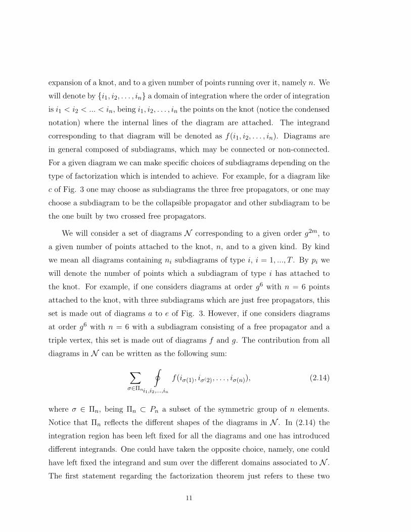
corresponding to that diagram will be denoted as f(i1, i2, . . . , in). Diagrams are

in general composed of subdiagrams, which may be connected or non-connected.

For a given diagram we can make specific choices of subdiagrams depending on the

type of factorization which is intended to achieve. For example, for a diagram like

c of Fig. 3 one may choose as subdiagrams the three free propagators, or one may

choose a subdiagram to be the collapsible propagator and other subdiagram to be

the one built by two crossed free propagators.

We will consider a set of diagrams N corresponding to a given order g2m, to

a given number of points attached to the knot, n, and to a given kind. By kind

we mean all diagrams containing ni subdiagrams of type i, i = 1, ..., T . By pi we

will denote the number of points which a subdiagram of type i has attached to

the knot. For example, if one considers diagrams at order g6 with n = 6 points

attached to the knot, with three subdiagrams which are just free propagators, this

set is made out of diagrams a to e of Fig. 3. However, if one considers diagrams

at order g6 with n = 6 with a subdiagram consisting of a free propagator and a

triple vertex, this set is made out of diagrams f and g. The contribution from all

diagrams in N can be written as the following sum:

∑

σ∈Πn

∮

i1,i2,...,in

f(iσ(1), iσ(2), . . . , iσ(n)), (2.14)

where σ ∈ Πn, being Πn ⊂ Pn a subset of the symmetric group of n elements.

Notice that Πn reflects the different shapes of the diagrams in N . In (2.14) the

integration region has been left fixed for all the diagrams and one has introduced

different integrands. One could have taken the opposite choice, namely, one could

have left fixed the integrand and sum over the different domains associated to N .

The first statement regarding the factorization theorem just refers to these two

11

possible choices. Let us define the domain resulting of permuting {i1, i2, . . . , in}by an element σ of the symmetric group Pn by

Dσ = { iσ(1), iσ(2), . . . , iσ(n) }, (2.15)

then the following result immediately follows.

Statement 1: The contribution to the Wilson line of the sum of diagrams whose

integrands are of the form:

f(iσ(1), iσ(2), . . . , iσ(n)), (2.16)

where σ runs over a given subset Πn ∈ Pn with a common domain of integration

is equal to the sum of the integral of f(i1, i2, . . . , in) over Dσ where σ ∈ Π−1n :

∮

i1,i2,...,in

∑

σ∈Πn

f(iσ(1), iσ(2), . . . , iσ(n)) =∑

σ∈Π−1n

∮

Dσ

f(i1, i2, . . . , in). (2.17)

The idea behind the factorization theorem is to organize the diagrams in N in

such a way that one is summing over all possible permutations of domains. Sum-

ming over all domains implies that one can consider the integration over the points

corresponding to each subdiagram as independent and therefore one can factor-

ize the contribution into a product given by the integrations of each subdiagram

independently. This leads to the following statement.

Statement 2: (Factorization theorem) Let Π′n be the set of all possible permu-

tations of the domains of integration of diagrams containing subdiagrams of types

i = 1, ..., T. If Π−1n = Π′

n, the sum of integrals over Dσ, σ ∈ Π−1n , is the product of

the integrals of the subdiagrams over the knot, being the domains all independent,

∑

σ∈Π−1n

∮

Dσ

f(i1, . . . , in) =

T∏

i=1

(∮

i1,...,ipi

fi(i1, . . . , ipi)

)ni

. (2.18)

In (2.18) ni denotes the number of subdiagram of type i and pi its number of points

attached to the knot.

12

The proof of this statement is trivial since having all possible domains it is

clear that one can write the integration considering subdiagram by subdiagram,

the result being the product of all the partial integrations over subdiagrams.

As a consequence of the factorization theorem we can state two corollaries

about the framing independence of diagrams which do not contain one-particle ir-

reducible subdiagrams corresponding to two-point functions whose endpoints could

get together. These corollaries refer to any kind of knot. Their statements are:

Framing dependent diagrams: A diagram gives a framing dependent contribu-

tion to the perturbative expansion of the knot if and only if it contains at least one

collapsible propagator. Moreover, the order of m in its contribution, the self-linking

number, equals the number of collapsible propagators.

Factorization of the framing dependence: If all the contribution to the self-

energy comes from one loop diagrams, then⟨

WRC

⟩

= F (C, R)e2πimhR where

F (C, R) is framing independent but knot dependent, and the exponential is man-

ifestly framing dependent but knot independent.

The quantities hR and m appearing in the framing dependence factor are, re-

spectively, the conformal weight associated to the representation R, and the integer

which labels the framing (self-linking number). The standard framing corresponds

to m = 0. The factorization of the framing dependence was proven in [43] for

SU(N) in the fundamental representation but it is obvious from the proof that it

generalizes for any representation of any semisimple group. We end this section

recalling that a full account of these results can be found in [43]. They are the cor-

nerstones of our approach to the finite-type invariants associated to perturbative

Chern-Simons theory.

13

3. General structure of the perturbative expansion

In this section we will analyze the structure of the perturbative series expansion

associated to Chern-Simons gauge theory with an arbitrary compact semisimple

gauge group G. We will discuss the general form of this series and we will present

its exact form up to order six. Let us consider the vacuum expectation value of the

Wilson line (2.13) corresponding to an arbitrary knot in an arbitrary representation

R of G. The contour integral in (2.13) corresponds to any path diffeomorphic to the

knot. To compute the vacuum expectation values of this operator in perturbation

theory we have to consider all diagrams which are not vacuum diagrams since

we consider normalized vacuum expectation values, i.e., the functional integration

where the operator is inserted is divided by the partition function Z as in (2.2).

Also, we will not consider diagrams which include collapsible propagators because

they only contribute to the dependence of the vacuum expectation value of W

on the framing. Finally we can omit the insertion of loops in every two and

three-point subdiagram since, as stated before, their only effect is to provide the

shift k→k − cA. We stress these two last points because they greatly simplify the

perturbative series. The framing and the shift are viewed as objects not intrinsic

to the knot and are therefore ignored.

From the Feynman rules presented in the previous section follows that the

perturbative expansion of the vacuum expectation value of the Wilson line operator

(2.13) has the form,

〈WRC 〉 = d(R)

∞∑

i=0

di∑

j=1

αijrijxi, (3.1)

where x = 2πik = ig2/2 is the expansion parameter, d(R) is the dimension of

the representation R, and α0,1 = r0,1 = 1, d0 = 1 and d1 = 0. Notice that

we are dispensing with the shift and the framing factor: only k appears in the

denominator of x and there is no linear term in the expansion (d1 = 0)⋆. The

⋆ At order x there is only the contribution from a diagram containing one collapsible propaga-

tor which according to the results presented in the previous section corresponds to framing.

14

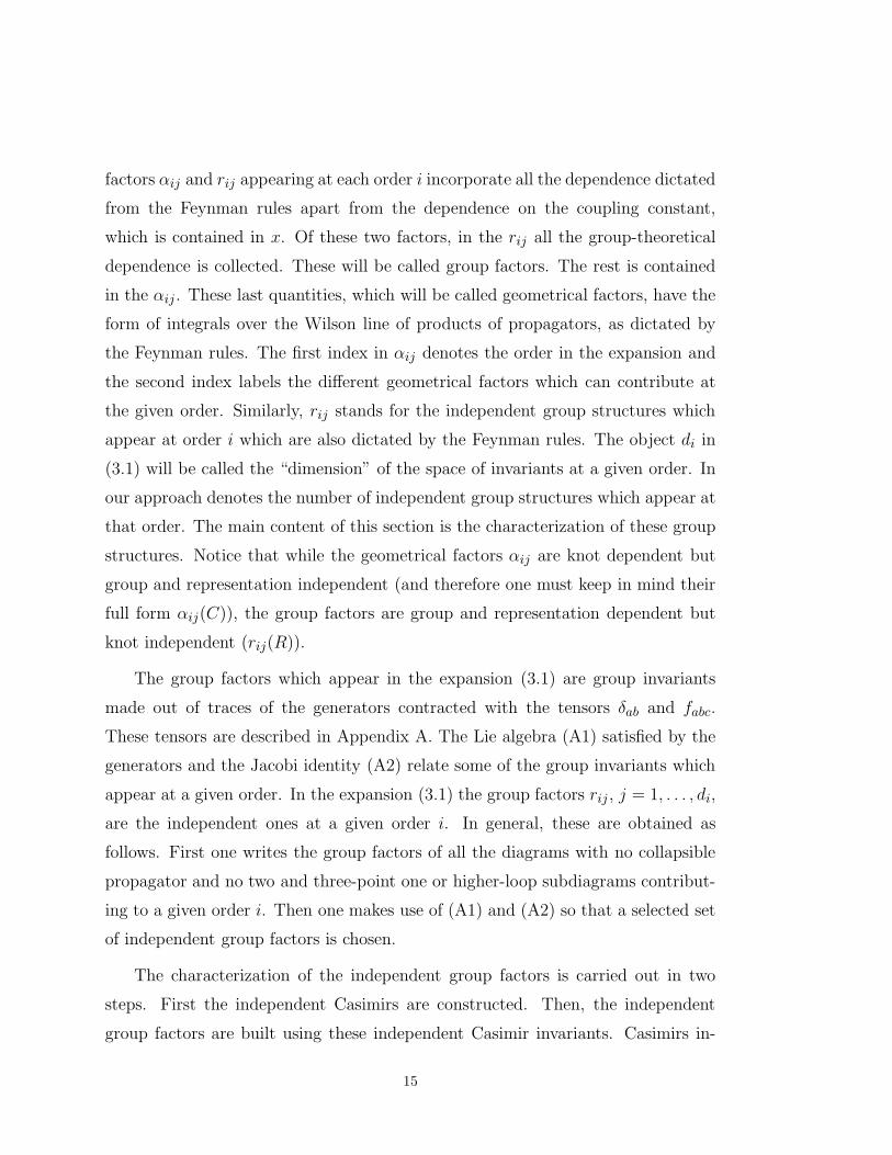
factors αij and rij appearing at each order i incorporate all the dependence dictated

from the Feynman rules apart from the dependence on the coupling constant,

which is contained in x. Of these two factors, in the rij all the group-theoretical

dependence is collected. These will be called group factors. The rest is contained

in the αij . These last quantities, which will be called geometrical factors, have the

form of integrals over the Wilson line of products of propagators, as dictated by

the Feynman rules. The first index in αij denotes the order in the expansion and

the second index labels the different geometrical factors which can contribute at

the given order. Similarly, rij stands for the independent group structures which

appear at order i which are also dictated by the Feynman rules. The object di in

(3.1) will be called the “dimension” of the space of invariants at a given order. In

our approach denotes the number of independent group structures which appear at

that order. The main content of this section is the characterization of these group

structures. Notice that while the geometrical factors αij are knot dependent but

group and representation independent (and therefore one must keep in mind their

full form αij(C)), the group factors are group and representation dependent but

knot independent (rij(R)).

The group factors which appear in the expansion (3.1) are group invariants

made out of traces of the generators contracted with the tensors δab and fabc.

These tensors are described in Appendix A. The Lie algebra (A1) satisfied by the

generators and the Jacobi identity (A2) relate some of the group invariants which

appear at a given order. In the expansion (3.1) the group factors rij , j = 1, . . . , di,

are the independent ones at a given order i. In general, these are obtained as

follows. First one writes the group factors of all the diagrams with no collapsible

propagator and no two and three-point one or higher-loop subdiagrams contribut-

ing to a given order i. Then one makes use of (A1) and (A2) so that a selected set

of independent group factors is chosen.

The characterization of the independent group factors is carried out in two

steps. First the independent Casimirs are constructed. Then, the independent

group factors are built using these independent Casimir invariants. Casimirs in-

15

variants will be denoted by Cji , where the subindex denotes the order of the Casimir

and the superindex labels the different Casimirs that appear at a given order. It

is worth to recall here that the order i of a Casimir is such that 2i equals the

number of generators plus the number of structure constants which appear in its

expression. The independent Casimirs for a semisimple group up to order 6 turn

out to be the following:

C ′2d(R) = fapqfbqpTr(TaTb),

C ′3d(R) = fapqfbqrfcrpTr(TaTbTc),

C4d(R) = fapqfbqrfcrsfdspTr(TaTbTcTd),

C5d(R) = fapqfbqrfcrsfdstfetpTr(TaTbTcTdTe),

C16d(R) = fapqfbqrfcrsfdstfetufrupTr(TaTbTcTdTeTr),

C26d(R) = fapqfbrsfctpfdurfeqsfgtuTr(TaTbTcTdTeTg).

(3.2)

Several comments are in order. First, in general, if there is only one Casimir at a

given order we will label it by Ci instead of C1i . Second, notice that the first two

have been denoted by C ′2 and C ′

3 instead of C2 and C3. The reason for this is that

the notation C2 and C3 will be reserved to these two Casimirs times appropriate

factors. This will simplify the expressions for the group factors. Third, the factor

d(R), the dimension of the representation, is introduced for convenience. Notice

that for an irreducible representation there is a trace of the identity matrix on the

right hand side. Fourth, it is at order 6 when two independent Casimirs appear for

the first time. Notice that for a specific semisimple group these two Casimirs might

not be independent. However, in general they are. What is meant by independence

is that C16 can not be written in terms of C2

6 plus terms which are products of lower

order Casimirs making use of (A1) and (A2). The number of independent Casimirs

at order i will be denoted by ci. We have c2 = c3 = c4 = c5 = 1 and c6 = 2. The

specific values of the independent Casimirs in (3.2) are given in Appendix A for

the groups SU(N) and SO(N) in their fundamental representations and for SU(2)

in an arbitrary irreducible representation.

16

As announced above, the second and third order Casimirs will be redefined for

later convenience. First notice that using (A2) and (A5) one finds,

C ′2d(R) = CATr(TaTa),

C ′3d(R) = −1

2CAfabcTr(TaTbTc),

(3.3)

where CA is the quadratic Casimir in the adjoint representation. On the other

hand, as it will become clear below, the two traces on the right hand side of (3.3)

are the quantities which more often appear in group factors. We then define,

C2 =1

d(R)Tr(TaTa) = C ′

2/CA, C3 = − 1

d(R)fabcTr(TaTbTc) = 2C ′

3/CA. (3.4)

The diagrams associated to the independent Casimirs C2, C3, C4, C5, C16 and C2

6

are shown in Fig.4. From those diagrams one easily writes down the Casimirs using

only the part of the Feynman rules concerning group-theoretical factors.

To obtain the group factors rij , j = 1, . . . , di, to a given order one must consider

all the diagrams with no collapsible propagators and no two and three-point loop-

insertions, and write their group factors in terms of the independent Casimirs

and products or ratios of them. We will present an algorithm which leads to the

independent group factors at a given order. We will discuss first the case of simple

groups and then we will generalize it for the semisimple case.

We will introduce first some notation. Let us consider an arbitrary diagram

D of the perturbative expansion. We will denote by V the number of vertices, by

Pfree the number of free propagators and by PI the number of “internal” propa-

gators with both endpoints attached to vertices present in a given diagram. It is

convenient to define he number of “effective” propagators, P , as,

P = 2V − PI + Pfree. (3.5)

It is also useful to introduce a grading p(i) for the Casimirs of order i, Cki ,

k = 1, . . . , ci, equal to the effective number of propagators corresponding to their

17

associated diagram (see Fig. 4).

p(2) = 1, p(3) = 2, p(i) = i if i ≥ 4. (3.6)

The main result leading to the characterization of group factors for the case of

simple groups is the following. Given a diagram D with P ≥ 3 effective propaga-

tors, its group-theoretical dependence takes the form,

r(D) =∑

{SP }

aSP

P∏

i=2

ci∏

k=1

(

Cki

)S(i,k), (3.7)

where the sum runs over all possible sets {SP } which we are about to define, and

aSPare some rational numbers depending on the diagram D. The sets {SP } are

all the possible collections of integers {S(i, k) : 2 ≤ i ≤ P, 1 ≤ k ≤ ci} satisfying

the following conditions:

P∑

i=2

ci∑

k=1

p(i)S(i, k) =P,

S(i, k) ≥0 if i 6= 2,

S(2, 1) + S(3, 1) ≥0,

S(2, 1) ≥2 − P.

(3.8)

According to (3.7), the integers S(i, k) correspond to the number of times that

the subdiagram associated to the Casimir Cki appears. The meaning of conditions

(3.8) is the following. The first one simply imposes that the total number of

effective propagators is correct, and the second one requires that for i 6= 2 the

subdiagrams corresponding to the Casimirs Cki appear a positive number of times.

The possible negative values of the S(i, k) for i = 2 are due to the presence of CA

factors, as explained below. Finally, the last two inequalities are the constraints

on these values. Notice that we have used the fact that c2 = c3 = 1. The formula

(3.7) is valid for P ≥ 3. The group structures corresponding to P = 2 must

18

be obtained independently. However, as discussed below, these are very simple.

Finally, we must mention that (3.7) provides all the group structures, including

the ones contributing to framing. These will be identified and discarded thereafter.

The proof of (3.7) goes by induction in P . Assume that we are given a diagram

Dp with P = p as the one depicted in Fig. 5 and that its group factor is r(Dp)

according to (3.7).

Now one more free propagator is introduced, and the key idea is to move one of its

endpoints next to the other by means of the commutation relations. This produces

a series of diagrams with p+1 effective propagators. The last element of this series

would include a diagram similar to Fig. 5 with a collapsible propagator included,

as the one depicted in Fig. 6. Its group factor will be C2 r(Dp).

According to our general framework, this is a framing dependent contribution

which should be set to zero, but we are interested only in group factors at this

moment. The remaining diagrams can be represented as the one in Fig.7.

The next step is based on the observation of the fact that all diagrams like Fig.

7 have a vertex with two points attached to the Wilson line. Again the procedure

employs the commutation relations in order to make these points closer until we

finish in a diagram with a “fishtail” like the one on the left of Fig. 8. By fishtail

we mean a configuration of internal lines in a diagram such the two propagators

attached contiguously to the Wilson line are joined to the same vertex. The other

diagrams generated are similar to the one on the right in the same figure.

As explained in Appendix B fishtails amount to a factor CA/2 = −C3/C2 and

therefore the group factor corresponding to the first diagram in Fig. 8 can be

written as −(C3/C2) r(Dp). The general procedure reproduces this scheme. Take

one of the vertices generated in the previous steps such that it has two points

connected to the Wilson line and move them until one gets a fishtail. Then repeat

the same routine with the diagrams arisen due to those movings. The procedure

finishes when one is left with diagrams such that all vertices have at most one

point on the Wilson line. This describes a diagram with closed loops which can

19

be connected or disconnected, as is schematically shown in Fig. 9. In the first

case it can be written as a combination of the Casimirs in Cip+1 and in the second

as a combination of products of lower Casimirs with a total number of effective

propagators equal to p + 1. These diagrams will be referred to as “Casimir-like”.

The result is that the group factors needed for r(Dp+1) are constructed by mul-

tiplying those of r(Dp) by C2 or C3/C2, by considering products of lower Casimirs

with a total number of effective propagators equal to p + 1, and by including the

new Casimirs Ckp+1. In our notation this means that P can be increased in one unit

only by some of the following procedures: adding 1 to S(2, 1); adding 1 to S(3, 1)

and −1 to S(2, 1); giving values to the S(i, k) corresponding to lower Casimirs in

such a way that the number of effective propagators equals p + 1; finally, setting

S(p + 1, k) = 1 (only one k at a time) for the new Casimirs. This is verified by

(3.7) for P = p + 1 if the numbers S(i, k) satisfy (3.8).

To end the proof of (3.7) we must present the group structures for the case

P = 3. Let us discuss first, as promised, the ones for P = 2. This offers no

difficulty because this case is nearly trivial. The diagrams contributing for P = 2

are the ones in Fig. 10 plus the diagram containing two collapsible propagators,

which has not been pictured. The calculation of the group factors corresponding

to these diagrams is rather straightforward and they turn out to be (C2)2 and C3.

For P = 3 one has group factors from the diagrams presented in Fig. 3. Although

a larger set than in the P = 2 case, their group factors are also computed very

easily. The independent ones are:

P = 3 : (3, 0) −→(

∑

C2

)3

(1, 1) −→(

∑

C2

)

∑

C3

(−1, 2) −→∑

[(

C2

)−1(C3

)2] ∗

where we have used the symbol∑

Cki as a shorthand for

∑nl=1 C

k (l)i . A similar

condensed notation will be adopted in the examples presented below. An asterisk

signals the group factors which contribute to the framing independent part. It

20

follows from the structure of the proof that these will be all group factors which do

not contain positive powers of∑

C2. The numerical sequence written on the left

of the group factors correspond to the set of integers S(i, k). Clearly, they satisfy

(3.8) and the proof of (3.7) is completed.

The generalization to the semisimple case can be treated as follows. It may

happen that different diagrams lead to the same group structure in the simple case.

This is explained in Appendix B. In (3.7) the products of Casimirs can sometimes

be separated in subproducts in such a way that each subproduct corresponds to

a possible subdiagram. These decompositions would yield all diagrams which in

the simple case have the same group factor. If the algebra is now A = ⊕nl=1Al

the Casimirs are Cki =

∑nl=1 C

k (l)i , and we can put the sum over l in front of

each subproduct for each of the decompositions. This would enlarge the number

of independent group structures.

Each of the subproducts appearing in a group factor corresponding to a given

number of effective propagators P verifies again (3.8) but with a smaller P , namely

P j. If the number of subproducts is s it has to be satisfied that,

s∑

j=1

P j = P. (3.9)

It should be noted that if the number ci in (3.8) and (3.7) were known, our

construction would provide a systematic method to compute the dimension di. The

numbers ci can probably be calculated by purely group-theoretical methods. We

leave this problem open for future work.

To clarify how (3.7) and the algorithm implicit in the proof works, some exam-

ples are in order. We will present explicit calculations of the sequences {SP }for P ≤ 6, including their corresponding factors rij , which can be read from

(3.7). As in the case P = 3, we will write integer sequences following the pat-

tern (S(2, 1), S(3, 1), S(4, 1), S(5, 1), [S(6, 1), S(6, 2)], . . .), i.e., in growing order in

i and for a given i in growing order in k. The S(i, k) corresponding to a given i will

21

be gathered inside square brackets. As used above, an asterisk will indicate that

the corresponding group structure contributes to the framing independent part.

The case P = 4 is the first one which follows the algorithm. The sequences

S(i, k) are the only possible ones verifying (3.8), and can be constructed starting

from the data for P = 3 either by adding 1 to S(2, 1) or by adding −1 to S(2, 1)

and 1 to S(3, 1). In addition, the third possibility pointed out in the proof of

(3.7) has to be taken into account because there is a Casimir corresponding to four

effective propagators, C4, and therefore the sequence (0, 0, 1) must be included:

P = 4 : (4, 0, 0) −→(

∑

C2

)4

(2, 1, 0) −→(

∑

C2

)2∑

C3

(0, 2, 0) −→{

(∑

C3

)2 ∗(∑

C2

)∑[(

C2

)−1(C3

)2]

(−2, 3, 0) −→∑

[(

C2

)−2(C3

)3] ∗

(0, 0, 1) −→∑

C4 ∗

Notice that the sequence (0, 2, 0) contains more than one group structure. This

happen after using the generalization of the algorithm for the semisimple case

which has been described. If the algebra were simple these multiple structures

would reduce to only one, as can be seen after suppressing the sums over the sim-

ple components of the algebra. To cope with these multiplicities we follow the

procedure outlined in the generalization of the algorithm to semisimple algebras.

First one writes the group structures corresponding to the simple case. These are:(

C2

)4,(

C2

)2C3,

(

C3

)2,(

C2

)−2(C3

)3, C4. Then one considers all possible parti-

tions of the previous factors in such a way that the subfactors correspond to subdi-

agrams. These subfactors correspond to a smaller number of effective propagators,

as explained in (3.9). Once this is done, a sum over the simple components of the

algebra can be put in front of each subfactor. In the case at hand this can only

be done in(

C3

)2which can also be written as

[

C2

][(

C3

)2(C2

)−1]. Each of these

two partitions correspond to admissible decompositions in subdiagrams. The first

22

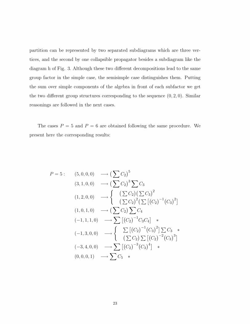
partition can be represented by two separated subdiagrams which are three ver-

tices, and the second by one collapsible propagator besides a subdiagram like the

diagram h of Fig. 3. Although these two different decompositions lead to the same

group factor in the simple case, the semisimple case distinguishes them. Putting

the sum over simple components of the algebra in front of each subfactor we get

the two different group structures corresponding to the sequence (0, 2, 0). Similar

reasonings are followed in the next cases.

The cases P = 5 and P = 6 are obtained following the same procedure. We

present here the corresponding results:

P = 5 : (5, 0, 0, 0) −→(

∑

C2

)5

(3, 1, 0, 0) −→(

∑

C2

)3∑

C3

(1, 2, 0, 0) −→{

(∑

C2

)(∑

C3

)2

(∑

C2

)2(∑[(

C2

)−1(C3

)2]

(1, 0, 1, 0) −→(

∑

C2

)

∑

C4

(−1, 1, 1, 0) −→∑

[(

C2

)−1C3C4

]

∗

(−1, 3, 0, 0) −→{

∑[(

C2

)−1(C3

)2]∑C3 ∗

(∑

C2

)∑[(

C2

)−2(C3

)3]

(−3, 4, 0, 0) −→∑

[(

C2

)−3(C3

)4] ∗

(0, 0, 0, 1) −→∑

C5 ∗

23

P = 6 : (6, 0, 0, 0, [0, 0]) −→(

∑

C2

)6

(4, 1, 0, 0, [0, 0]) −→(

∑

C2

)4∑

C3

(2, 2, 0, 0, [0, 0]) −→{

(∑

C2

)2(∑C3

)2

(∑

C2

)3∑[(

C2

)−1(C3

)2]

(2, 0, 1, 0, [0, 0]) −→(

∑

C2

)2∑

C4

(1, 0, 0, 1, [0, 0]) −→(

∑

C2

)

∑

C5

(0, 3, 0, 0, [0, 0]) −→

(∑

C3

)3 ∗(∑

C2

)(∑

C3

)∑[(

C2

)−1(C3

)2]

(∑

C2

)2∑[(

C2

)−2(C3

)3]

(0, 1, 1, 0, [0, 0]) −→{

(∑

C3

)∑

C4 ∗(∑

C2

)∑[(

C2

)−1C3C4

]

(−1, 1, 0, 1, [0, 0]) −→∑

[(

C2

)−1C3C5

]

∗

(−2, 2, 1, 0, [0, 0]) −→∑

[(

C2

)−2(C3

)2C4

]

∗

(−2, 4, 0, 0, [0, 0]) −→

(∑

C2

)∑[(

C2

)−3(C3

)4]

(∑

C3

)∑[(

C2

)−2(C3

)3] ∗(∑[(

C2

)−1(C3

)2])2 ∗(−4, 5, 0, 0, [0, 0]) −→

∑

[(

C2

)−4(C3

)5] ∗

(0, 0, 0, 0, [1, 0]) −→∑

C16 ∗

(0, 0, 0, 0, [0, 1]) −→∑

C26 ∗

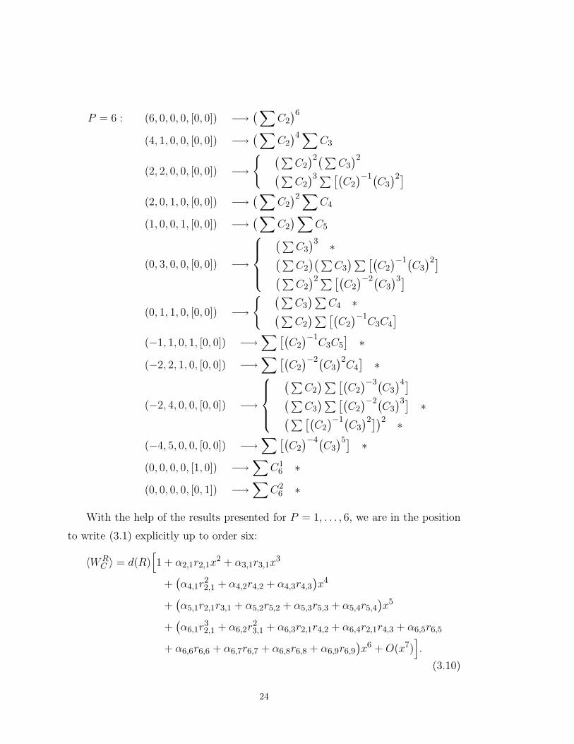
With the help of the results presented for P = 1, . . . , 6, we are in the position

to write (3.1) explicitly up to order six:

〈WRC 〉 = d(R)

[

1 + α2,1r2,1x2 + α3,1r3,1x

3

+(

α4,1r22,1 + α4,2r4,2 + α4,3r4,3

)

x4

+(

α5,1r2,1r3,1 + α5,2r5,2 + α5,3r5,3 + α5,4r5,4

)

x5

+(

α6,1r32,1 + α6,2r

23,1 + α6,3r2,1r4,2 + α6,4r2,1r4,3 + α6,5r6,5

+ α6,6r6,6 + α6,7r6,7 + α6,8r6,8 + α6,9r6,9

)

x6 + O(x7)]

.

(3.10)

24

The group factors rij can be read from the listed results above. These can be

classified in two types, the ones which are not products of lower order group factors,

r2,1 =

n∑

k=1

C(k)3 ,

r3,1 =

n∑

k=1

(

C(k)3

)2(C

(k)2

)−1,

r4,2 =n∑

k=1

(

C(k)3

)3(C

(k)2

)−2,

r4,3 =n∑

k=1

C(k)4 ,

r5,2 =

n∑

k=1

(

C(k)3

)4(C

(k)2

)−3,

r5,3 =

n∑

k=1

C(k)4 C

(k)3

(

C(k)2

)−1,

r5,4 =

n∑

k=1

C(k)5 ,

r6,5 =

n∑

k=1

(

C(k)3

)5(C

(k)2

)−4,

r6,6 =n∑

k=1

C(k)4

(

C(k)3

)2(C

(k)2

)−2,

r6,7 =n∑

k=1

C(k)5 C

(k)3

(

C(k)2

)−1,

r6,8 =

n∑

k=1

C1 (k)6 ,

r6,9 =

n∑

k=1

C2 (k)6 ,

(3.11)

and the ones which are products of lower order ones,

r4,1 =r22,1,

r5,1 =r2,1r3,1,

r6,1 =r32,1,

r6,2 =r23,1,

r6,3 =r2,1r4,2,

r6,4 =r2,1r4,3.

(3.12)

In Fig. 11 a representative diagram for each of these group factors has been

pictured. These are easily obtained from (3.11) and (3.12) after taking into account

the diagrams corresponding to the independent Casimirs drawn in Fig. 4.

From the results (3.11) and (3.12) one can read off the values of the dimensions

di for i = 1 to 6:

d = 0, 1, 1, 3, 4, 9. (3.13)

The value d1 = 0 was implicit in (3.10) and its origin resides on the absence of the

term linear in x in that equation, which is due to the withdrawal of the framing.

25

The expansion (3.1) verifies a basic property closely related to the factorization

theorem. If we denote by 〈WRk

C 〉 and 〈WRC 〉 the vacuum expectation values of

Wilson lines based on the algebras Ak and A = ⊕nk=1Ak, being the representation

R a direct product of representations Rk, it turns out that,

〈WRC 〉 =

n∏

k=1

〈WRk

C 〉. (3.14)

This follows directly from the factorization of both the partition function and the

Wilson line operator. Comparing both sides of (3.14) some relations among the

geometric coefficients in their corresponding expansions (3.1) appear, which can

be also derived after knowing their explicit form by means of the factorization

theorem:

α4,1 =1

2α2

2,1,

α5,1 =α2,1α3,1,

α6,1 =1

6α3

2,1,

α6,2 =1

2α2

3,1,

α6,3 =α2,1α4,2,

α6,4 =α2,1α4,3.

(3.15)

These relationships hold also if the Wilson line corresponding to the knot under

consideration is normalized by the Wilson line of the unknot, although the specific

values of the αij change. This will be proven in the next section. These properties

are explicitly checked in several examples in the next section.

26

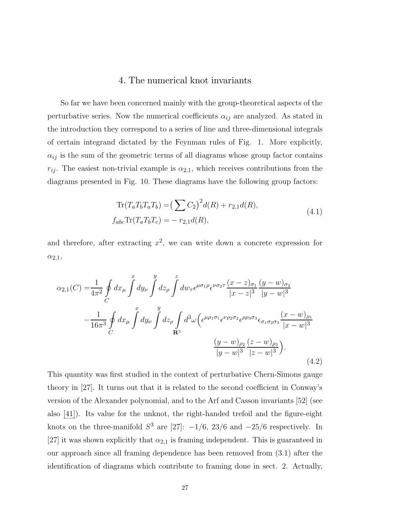
4. The numerical knot invariants

So far we have been concerned mainly with the group-theoretical aspects of the

perturbative series. Now the numerical coefficients αij are analyzed. As stated in

the introduction they correspond to a series of line and three-dimensional integrals

of certain integrand dictated by the Feynman rules of Fig. 1. More explicitly,

αij is the sum of the geometric terms of all diagrams whose group factor contains

rij . The easiest non-trivial example is α2,1, which receives contributions from the

diagrams presented in Fig. 10. These diagrams have the following group factors:

Tr(TaTbTaTb) =(

∑

C2

)2d(R) + r2,1d(R),

fabcTr(TaTbTc) = − r2,1d(R),(4.1)

and therefore, after extracting x2, we can write down a concrete expression for

α2,1,

α2,1(C) =1

4π2

∮

C

dxµ

x∫

dyν

y∫

dzρ

z∫

dwτ ǫµσ1ρǫνσ2τ (x − z)σ1

|x − z|3(y − w)σ2

|y − w|3

− 1

16π3

∮

C

dxµ

x∫

dyν

y∫

dzρ

∫

R3

d3ω(

ǫµρ1σ1ǫνρ2σ2ǫρρ3σ3ǫσ1σ2σ3

(x − w)ρ1

|x − w|3

(y − w)ρ2

|y − w|3(z − w)ρ3

|z − w|3)

.

(4.2)

This quantity was first studied in the context of perturbative Chern-Simons gauge

theory in [27]. It turns out that it is related to the second coefficient in Conway’s

version of the Alexander polynomial, and to the Arf and Casson invariants [52] (see

also [41]). Its value for the unknot, the right-handed trefoil and the figure-eight

knots on the three-manifold S3 are [27]: −1/6, 23/6 and −25/6 respectively. In

[27] it was shown explicitly that α2,1 is framing independent. This is guaranteed in

our approach since all framing dependence has been removed from (3.1) after the

identification of diagrams which contribute to framing done in sect. 2. Actually,

27

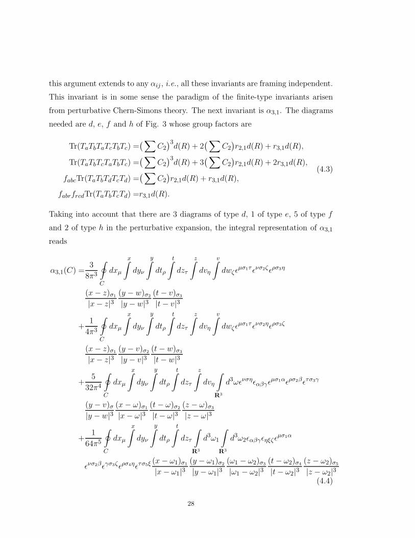
this argument extends to any αij , i.e., all these invariants are framing independent.

This invariant is in some sense the paradigm of the finite-type invariants arisen

from perturbative Chern-Simons theory. The next invariant is α3,1. The diagrams

needed are d, e, f and h of Fig. 3 whose group factors are

Tr(TaTbTaTcTbTc) =(

∑

C2

)3d(R) + 2

(

∑

C2

)

r2,1d(R) + r3,1d(R),

Tr(TaTbTcTaTbTc) =(

∑

C2

)3d(R) + 3

(

∑

C2

)

r2,1d(R) + 2r3,1d(R),

fabcTr(TaTbTdTcTd) =(

∑

C2

)

r2,1d(R) + r3,1d(R),

fabrfrcdTr(TaTbTcTd) =r3,1d(R).

(4.3)

Taking into account that there are 3 diagrams of type d, 1 of type e, 5 of type f

and 2 of type h in the perturbative expansion, the integral representation of α3,1

reads

α3,1(C) =3

8π3

∮

C

dxµ

x∫

dyν

y∫

dtρ

t∫

dzτ

z∫

dvη

v∫

dwζǫµσ1τ ǫνσ2ζǫρσ3η

(x − z)σ1

|x − z|3(y − w)σ2

|y − w|3(t − v)σ3

|t − v|3

+1

4π3

∮

C

dxµ

x∫

dyν

y∫

dtρ

t∫

dzτ

z∫

dvη

v∫

dwζǫµσ1τ ǫνσ2ηǫρσ3ζ

(x − z)σ1

|x − z|3(y − v)σ2

|y − v|3(t − w)σ3

|t − w|3

+5

32π4

∮

C

dxµ

x∫

dyν

y∫

dtρ

t∫

dzτ

z∫

dvη

∫

R3

d3ωǫνσηǫαβγǫµσ1αǫρσ2βǫτσ3γ

(y − v)σ|y − w|3

(x − ω)σ1

|x − ω|3(t − ω)σ2

|t − ω|3(z − ω)σ3

|z − ω|3

+1

64π5

∮

C

dxµ

x∫

dyν

y∫

dtρ

t∫

dzτ

∫

R3

d3ω1

∫

R3

d3ω2ǫαβγǫηξζǫµσ1α

ǫνσ2βǫγσ3ζǫρσ4ηǫτσ5ξ (x − ω1)σ1

|x − ω1|3(y − ω1)σ2

|y − ω1|3(ω1 − ω2)σ3

|ω1 − ω2|3(t − ω2)σ4

|t − ω2|3(z − ω2)σ5

|z − ω2|3(4.4)

28

An important property of the geometrical factors αij is their behavior under

changes of orientation in the manifold. Notice that while α2,1 possesses a product

of an even number of three-dimensional totally antisymmetric tensors in all its

terms, α3,1 has a product of an odd number. Thus, under a change of orientation

α2,1 is even and α3,1 is odd. From the Feynman rules of the theory follows that,

in general, for even i the factors αij are even under a change of orientation while

for odd i those factors are odd. This implies that a knot K and its mirror image

K have geometrical factors such that

αij(K) = αij(K), if i is even,

αij(K) = −αij(K), if i is odd.(4.5)

In particular, for amphicheiral knots (K ∼ K), αij(K) = 0 for i odd. Looking

back at the expansion (3.1) one observes that these results are in agreement with

the fact that for quantum group knot invariants, their value for knots related by a

change of orientation in the manifold are the same once the replacement q → q−1

is performed. Since q = ex, this is equivalent to carry out the change x → −x,

which, using (3.1) and the fact that the rij are knot independent implies (4.5).

It is possible to continue the procedure described above and give the expressions

which correspond to higher coefficients αij . One simply has to draw all diagrams

corresponding to the given order, compute their group factors in the way explained

above, gather the framing independent contributions and display an integral after

using the Feynman rules. Nevertheless the resulting expressions are somewhat

unwieldy and not too illuminating. We will instead study the properties of these

knot invariants.

The knot invariants αij can be written in many ways because their defining

expansion (3.1) is subject to two different types of normalizations. On the one

hand, the vacuum expectation value 〈WRC 〉 could be normalized differently. For

example, the choice made in (3.1) is such that it does not have value one for

the unknot. Dividing 〈WRC 〉 by the corresponding quantity for the unknot will

29

shift the values of the αij . On the other hand, the group factors depend on the

group theoretical conventions, in particular the normalization of the generators of

the semisimple group. Since 〈WRC 〉 is independent on how those generators are

normalized, the αij must be different for different normalizations. In more explicit

terms, the integral expressions obtained for α2,1 and for α3,1 in (4.2) and (4.4) would

contain different global factors. To make the knot invariants αij universal we will

first redefine them dividing by the unknot. This will fix the additive arbitrariness of

the αij and will impose the property that all these invariants vanish for the unknot.

Second, we will fix the multiplicative arbitrariness of the invariants αij by taking

the simplest non-trivial knot, the trefoil, and fixing the values of the invariants to

some selected integers. This can be done if all the invariants do not vanish for the

trefoil. This holds up to order six and we will assume that it holds in general. As

we will see in the next section the choice made supports the conjecture that it is

possible to find a normalization were all the invariant quantities are integers. This

is a highly non-trivial feature looking at their integral representations as the ones

in (4.2) and (4.4). In the next section we will present all these facts explicitly up

to order six for all prime knots up to six crossings.

Let us denote the unknot by U and let us consider its expansion (3.1),

〈WRU 〉 = d(R)

∞∑

i=0

di∑

j=1

αij(U)rij(R)xi. (4.6)

Let us now consider un arbitrary knot K. We define the new knot invariants

αij(K) normalizing by the expression for the unknot:

〈WRK〉

〈WRU 〉 =

∑∞i=0

∑di

j=1 αij(K)rij(R)xi

∑∞i=0

∑di

j=1 αij(U)rij(R)xi=

∞∑

i=0

di∑

j=1

αij(K)rij(R)xi. (4.7)

Similarly to the case of (3.1), one has α0,1 = 1. Notice that for the unknot, U , one

has αij(U) = 0, ∀ i, j, such that i 6= 0. From the values given above for α2,1 for the

unknot, the right-handed trefoil and the figure-eight knot (−1/6, 23/6 and −25/6

30

respectively), one easily obtain the value of α2,1 for the right-handed trefoil and

the figure-eight knot: 23/6 + 1/6 = 4 and −25/6 + 1/6 = −4, respectively. It is

clear from (4.7) and the fact that the unknot is amphicheiral that the properties

(4.5) are also satisfied by the αij .

The new quantities αij(K) also satisfy relations as the ones in (3.15). To prove

this notice that relation (3.14) holds for any knot, in particular for the unknot.

This implies,

〈WRC 〉

〈WRU 〉 =

∏nk=1〈WRk

C 〉∏n

k=1〈WRk

U 〉=

n∏

k=1

〈WRk

C 〉〈WRk

U 〉, (4.8)

which, similarly to the case (3.15) leads to,

α4,1 =1

2α2

2,1,

α5,1 =α2,1α3,1,

α6,1 =1

6α3

2,1,

α6,2 =1

2α2

3,1,

α6,3 =α2,1α4,2,

α6,4 =α2,1α4,3.

(4.9)

The knot invariants αij , besides being topological invariants and framing in-

dependent, are also knot invariants of finite type in the sense of Vassiliev. This

follows from the results of [48], where the authors showed that the ith coefficient

of the expansion in x of the HOMFLY and Kauffman polynomials of an arbitrary

knot K, HN,q(K) and RN,q(K), after taking q = ex, is a Vassiliev invariant of order

i. The theorem was extended for an arbitrary quantum group invariant in [49]. It

is also presented in [41] and, in full generality, in [53]. We simply extend this result

to the different coefficients αij which contribute to the ith order in the expansion.

The idea is that at a given order the different structures rij are independent and

therefore all the αij are independent Vassiliev invariants of order i.

To be self-contained, we review very briefly the axiomatic approach to Vassiliev

invariants proposed in [48] and [53], where a thorough treatment of the subject can

be found. A j-singular knot is a knot which has j transversal self-intersections.

This object is denoted by Kj . The self-intersection can be made an undercrossing

31

or an overcrossing, which are called the resolutions of the self-intersection. Given

a knot invariant V (K) it can be extended to be an invariant of j-singular knots by

means of the prescription presented in Fig. 12.

The formula presented in Fig. 12 is the first axiom of Birman and Lin. If

we denote by Kj+ a j-singular knot with an overcrossing at a given point and by

Kj− the same with an undercrossing instead of the overcrossing, this axiom can be

written as a crossing-change formula,

V (Kj) = V (Kj−1+ ) − V (Kj−1

− ). (4.10)

The second axiom states that the Vassiliev invariants vanish on j-singular knots

for j high enough. In other words:

∃i ∈ Z+ such that V (Kj) = 0 if j > i. (4.11)

The smallest such i is called the order (or type) of V . A Vassiliev invariant of order

i will be denoted by Vi. Besides these two axioms, some initial data are needed.

Let us denote by U the unknot. Then one requires that all Vassiliev invariants of

U vanish,

Vi(U) = 0, ∀i ∈ Z+. (4.12)

A singular point p is called nugatory if its two resolutions define the same knot.

Let us denote by Kjp a singular knot which includes a nugatory point p. If we are

to obtain knot invariants, the following axiom has to be satisfied:

Vi(Kjp) = 0, if p is nugatory. (4.13)

A further set of initial data is needed to begin with the calculation of the invariants.

This corresponds to a set of given Vi(Kj) for some selected singular knots, presented

in the form of a table, called the actuality table. Of course these numbers are not

32

arbitrary and have to satisfy some rules in order to yield consistent values for the

numerical invariants. These consistency conditions are a system of linear equations,

where the unknowns are the numbers present in the actuality table. Birman and

Lin [48,53] proved that the expansion of any quantum group invariant associated to

a knot K yields consistent values for these numerical knot invariants, and therefore

are Vassiliev invariants. We will use this result to prove that the knot invariants

αij in (4.7) are Vassiliev invariants.

Let us consider a knot K. According to Birman and Lin [48,49], for any

semisimple group, one can assert that the contribution at each order in x in the

expansion (3.1),

Vi(K) =di∑

k=1

αik(K)rik, (4.14)

is a Vassiliev invariant of order i. This means that these Vi satisfy the axioms given

above. In other words, if one defines invariants for j-singular knots from (4.14)

using (4.10), one finds that (4.11), (4.12) and (4.13) hold, and that a consistent

actuality table is obtained. Following the same mechanism we define the αik(K)

for j-singular knots using (4.14) and (4.10). Indeed, in writing (4.10), one finds,

di∑

k=1

αik(Kj)rik =di∑

k=1

αik(Kj−1+ )rik −

di∑

k=1

αik(Kj−1− )rik, (4.15)

and then, from the independence of the group factors rik follows that,

αik(Kj) = αik(Kj−1

+ ) − αik(Kj−1− ). (4.16)

To prove that the quantities αik(Kj) defined in this way satisfy (4.11), (4.12)

and (4.13) we must take into account that, again, making use of the theorem by

Birman and Lin, Vi(Kj) =

∑di

k=1 αik(Kj)rik do satisfy these axioms. Writting

out the corresponding expressions in terms of this sum and making use of the

independence of the group factors follows that (4.11), (4.12) and (4.13) are also

33

verified by the quantities αik(Kj). Similarly, one concludes that given a type i

there is a consistent actuality table for each k, i.e., the αik generate an actuality

table once their value for j-singular knots is defined through (4.16). Therefore, the

geometrical factors associated to knots in (4.7) and their extension to j-singular

knots done in (4.16) are invariants of finite type or Vassiliev invariants. Notice that

these invariants generate di actuality tables for each i. The actuality table that

one would generate following Birman and Lin for a given quantum group invariant

would be a special linear combination of these di actuality tables.

Vassiliev invariants form an algebra, not just a sequence of vector spaces. Prod-

ucts of Vassiliev invariants of types i and j lead to Vassiliev invariants of type ij.

This structure is also manifest in our knot invariants due to relations (4.9). These

follow from the factorization property of Wilson lines for semisimple groups (3.14).

Invariants can in this way be classified in two types: simple invariants as the ones

which are not product of lower type invariants, and compound invariants which

are the rest. Taking into account (4.9), α2,1, α3,1, α4,2, α4,3, α5,2, α5,3, α5,4, α6,5,

α6,6, α6,7, α6,8 and α6,9 are simple invariants. The rest are compound invariants.

An important quantity is the number of simple invariants at each order or type.

We will denote it by di. For i = 1, . . . , 6 one finds,

d = 0, 1, 1, 2, 3, 5. (4.17)

One of the most important aspects of this work is that it provides a geometrical

interpretation of Vassiliev invariants in the sense that they are written as integra-

tions of the type (4.2) and (4.4) and their generalizations. It would be interesting to

study the relation between this integral representation and the one by Kontsevich

[54]. Our approach is intrinsic to three dimensions and can be easily generalized

to arbitrary three-manifold. In contrast, Kontsevitch’s representation is basically

two-dimensional (in the sense that the three-manifold is considered as a product

R×C) and therefore it is not obvious how to extend it to more general situations.

However, for the case in which Kontsevich representation is defined, they should

34

be related. This is supported by recent work [55] showing that Chern-Simons

gauge theory in the Hamiltonian formalism leads to Kontsevich representation for

Vassiliev invariants.

It is important at this point to discuss the relation between this work and the

one by Bar-Natan in [56]. In [56] it is proved that the group factors of all Feynman

diagrams with no collapsible propagators which contribute to a given order in g2

(or x) can be regarded as Vassiliev invariants. These Vassiliev invariants have an

entirely different origin than the knot invariants αik. Bar-Natan’s approach has

two steps. First the observation that one can associate Feynman-like diagrams

with no collapsible propagators to j-singular knots. Second that assigning the

group factors of these diagrams to j-singular knots one constructs a set of rational

numbers (weight system) that satisfies the axioms by Birman and Lin. Clearly,

this observation is orthogonal to our results. It is important, however, to notice

that the dimension of the space of Vassiliev invariants in [56] equals the number

of independent group structures and therefore must have the same values as our

di. Comparing the results in [56] with the values for di presented in (4.17) one

finds complete agreement up to i = 6. We think that the calculation of these

dimensions, in general, is more tractable in our approach. Recall that, as stated

in the previous section, after equation (3.7) and its generalization for semisimple

groups, the problem to compute di is reduced to the problem of finding ci, or

number of independent Casimirs of order i. The study of this issue is left for

future work.

Taking into account the work [56] there appears a very appealing situation. The

coefficient of xi in the expansion of any quantum group invariant can be regarded as

the inner product of two vectors of dimension di (the αik and the rik, k = 1, · · · , di).

Each of these two vectors is made out of Vassiliev invariants though each one has

a different interpretation: while the αik are associated to the non-singular knot

under study, the rik are in correspondence with a very precise set of j-singular

knots, and associated to the group and representation under consideration.

35

5. Numerical knot invariants for all prime knots up to six crossings

In this section we will present the calculation of the knot invariants αij for

all prime knots up to six crossings up to order six. Then we will show evidence

supporting that there exist a normalization such that these knot invariants are

integer-valued.

In order to compute the knot invariants αij(K) one could try to evaluate their

integral expressions. This is certainly a long and tedious way to proceed. There is

a faster way to carry out their computation using known information on the left

hand side of (4.7). Indeed, the knot invariant 〈WRK 〉/〈WR

U 〉 is known for a variety

of groups and representations for many knots on the three-manifold S3. Taking

its value for different cases one generates systems of linear equation where the

unknowns are the αij(K). Recall that while the rij(R) are group and represen-

tation dependent, they are knot independent. All dependence on K is contained

in αij(K) which, on the other hand, are independent of the group and the rep-

resentation. Up to order i = 6, which is the situation analyzed in this section,

it is enough to consider the following cases: SU(2) in an arbitrary representa-

tion of spin j (Jones and Akutsu-Wadati polynomials [20,21,24,14,18]), SU(N) in

the fundamental representation f (HOMFLY polynomial [22,21]), SO(N) in the

fundamental representation (Kauffman polynomial [23]), and SU(2) × SU(N) in

representations of the form (j, f), i.e., a representation of spin j in the subgroup

SU(2), and the fundamental in the subgroup SU(N). These invariants are known

and can be collected from the literature. They are listed in Appendix C.

The structure of the computation to be carried out is the following. Once the

polynomial invariant corresponding to the left hand side of (4.7) is collected one

replaces its variable q by ex and expands in powers of x. For the case considered

in this section one needs just the expansion up to order six. The coefficients of xi

are either polynomials in N , polynomials in j, or polynomials in N and j. On the

other hand, on the right hand side of (4.7) the group factors are the ones in (3.11)

and (3.12), which can be written explicitly using the values of the corresponding

36

Casimirs, which are listed in Appendix B. Again, one observes quickly that the

group factors are polynomials in N , j, or both, N and j. Both sides of (4.7) must

then be compared. This leads to series of linear equations which must be satisfied

by the αij(K). It turns out that one encounters 5 equations for α2,1(K), 5 equa-

tions for α3,1(K), 12 equations for α4,1(K), α4,2(K) and α4,3(K), 15 equations for

α5,1(K), . . ., α5,4(K), and 20 equations for α6,1(K), . . ., α6,9(K). Those equations

determine uniquely all the αij(K) up to order six.

The values of the αij(K) obtained in this way are, in general, rational numbers.

For the trefoil, which will be labeled in the standard form 31 [57], one finds,

α2,1(31) = 4,

α3,1(31) = 8,

α4,1(31) = 8,

α4,2(31) =62

3,

α4,3(31) =10

3,

α5,1(31) = 32,

α5,2(31) =176

3,

α5,3(31) =32

3,

α5,4(31) = 8,

α6,1(31) =32

3,

α6,2(31) = 32,

α6,3(31) =248

3,

α6,4(31) =40

3,

α6,5(31) =5071

30,

α6,6(31) =116

30,

α6,7(31) =3062

45,

α6,8(31) =17

18,

α6,9(31) =271

30.

(5.1)

Notice that these quantities satisfy the relations predicted in (4.9). We will not

present the values of the αij for other knots since we are going first to normalize

them properly.

As discussed in the previous section, these αij(K) are not universal in the sense

that they depend on the group theoretical conventions used. It should be desirable

to redefine them in such a way that they do not depend on those conventions. The

simplest way to proceed would be to decide that these knot invariants take the

37

value 1 for some knot in which none of them vanish. We will assume that this

non-vanishing feature occurs for the simplest knot, the trefoil. It is certainly true

up to order six as can be seen in (5.1). As we will show below, there is another

normalization possibility, which is the one that we will finally take, in which all

invariants up to order six seem to be integer-valued. Choosing the values for αij(31)

as some selected integers, it turns out that the resulting invariants are integers.

Our computations show that this happens to all prime knots up to six crossings.

This leads us to conjecture that a similar picture holds for all orders and all knots.

Let us first redefine the universal knot invariants. We will denote them by

βij(K) as,

βij(K) =αij(K)

αij(31). (5.2)

These invariants are well defined if the quantities αij(31) do not vanish. We will

assume this holds. On the other hand, it is clear from (5.2) that the invariants

βij(K) are independent of the normalization chosen for the Lie algebra generators.

There is certainly a dependence on the basis for group factors which has been

chosen but this dependence is intrinsic to their definition. For the right-handed

trefoil, βij(31) = 1. In this normalization the algebra (4.9) simplifies. Instead of

having numerical factors as the ones in (4.9) it turns out that just the product of

two invariants, one of order i and another of order j, leads to the corresponding

invariant of order ij.

Actually, it seems that there is a refined choice of the universal knot invariants

which makes them integer-valued. This choice can only be observed after com-

puting βij(K) for many knots. We have carried out their calculation for all prime

knots up to six crossings. The selected normalization up to order six is,

38

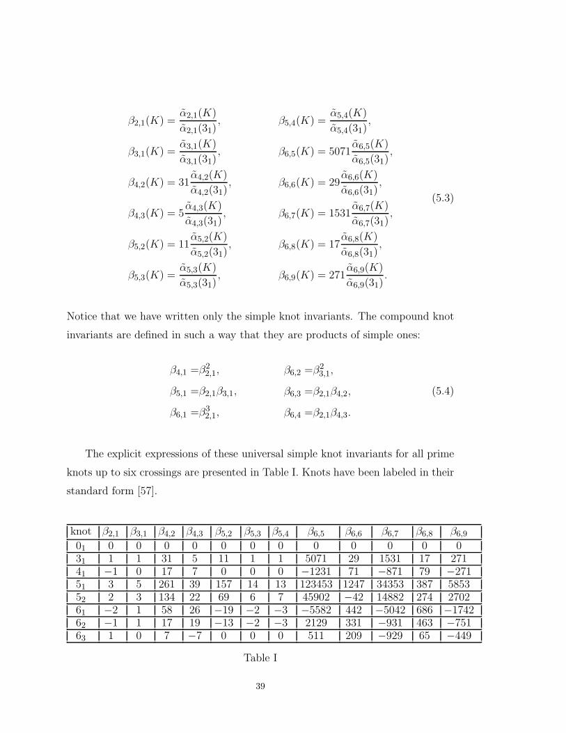
β2,1(K) =α2,1(K)

α2,1(31),

β3,1(K) =α3,1(K)

α3,1(31),

β4,2(K) = 31α4,2(K)

α4,2(31),

β4,3(K) = 5α4,3(K)

α4,3(31),

β5,2(K) = 11α5,2(K)

α5,2(31),

β5,3(K) =α5,3(K)

α5,3(31),

β5,4(K) =α5,4(K)

α5,4(31),

β6,5(K) = 5071α6,5(K)

α6,5(31),

β6,6(K) = 29α6,6(K)

α6,6(31),

β6,7(K) = 1531α6,7(K)

α6,7(31),

β6,8(K) = 17α6,8(K)

α6,8(31),

β6,9(K) = 271α6,9(K)

α6,9(31).

(5.3)

Notice that we have written only the simple knot invariants. The compound knot

invariants are defined in such a way that they are products of simple ones:

β4,1 =β22,1,

β5,1 =β2,1β3,1,

β6,1 =β32,1,

β6,2 =β23,1,

β6,3 =β2,1β4,2,

β6,4 =β2,1β4,3.

(5.4)

The explicit expressions of these universal simple knot invariants for all prime

knots up to six crossings are presented in Table I. Knots have been labeled in their

standard form [57].

knot β2,1 β3,1 β4,2 β4,3 β5,2 β5,3 β5,4 β6,5 β6,6 β6,7 β6,8 β6,9

01 0 0 0 0 0 0 0 0 0 0 0 031 1 1 31 5 11 1 1 5071 29 1531 17 27141 −1 0 17 7 0 0 0 −1231 71 −871 79 −27151 3 5 261 39 157 14 13 123453 1247 34353 387 585352 2 3 134 22 69 6 7 45902 −42 14882 274 270261 −2 1 58 26 −19 −2 −3 −5582 442 −5042 686 −174262 −1 1 17 19 −13 −2 −3 2129 331 −931 463 −75163 1 0 7 −7 0 0 0 511 209 −929 65 −449

Table I

39

The second row in Table I corresponds to the unknot, which has been labeled

by 01. This, as well as the second row, which corresponds to the trefoil, can be

thought as the choice of normalization. Once those are selected, the knot invariants

βij for all other knots are fixed and are independent of the normalization of the Lie

algebra generators. For knots which are chiral (not amphicheiral) we have selected

in Table I the one which has β3,1 > 0. Notice that, as discussed before, for the

two amphicheiral knots in the Table I, 41 and 63, one has βij = 0 for i odd. The

values β2,1(31), β2,1(41) and β2,1(51) can be checked with the explicit computation

of (4.2) in [27]. After taking into account the normalizations used in this work

one finds full agreement. It is important to remark that the quantities βij(K) are

intrinsic to the knot, i.e., as it follows from their construction they are framing

independent.

In Table I only the simple knot invariants have been listed. Vassiliev invariants

form an algebra [53] whose structure in the context of this work is represented

by relations (5.4). The compound knot invariants are given by those relations

from the values in Table I. The invariants constructed in this paper allow to build

actuality tables using (4.10). There is one actuality table, or one Vassiliev invariant,

associated to each βij , being this simple or compound. At a given type i, the space

of Vassiliev invariants has dimension mi, which at least up to i = 7 equals the

quantity di [56]. On the other hand, we have a way to generate di sets of Vassiliev

invariants or actuality tables. One could ask if the knot invariants constructed

are independent or not, i.e., if at each order they constitute a basis of Vassiliev

invariants. Up to order 5 this holds. At order 6 we do not have enough information

to come to a conclusion. The invariants should be computed for a higher number

of knots. We would like, however, to conjecture that at each order i, the knot

invariants proposed in this paper constitute a basis of Vassiliev invariants of type

i.

The values of the Vassiliev invariants presented in Table I can be contrasted

with the ones given in [46]. There, knots up to 7 crossings are considered, and

Vassiliev invariants are presented up to order 4. It turns out that β2,1 and β3,1 are

40

the same as in Table I. On the other hand, the three invariants of order 4 seem

rather different. To compare two presentations of Vassiliev invariants of a given

order one must take into account two facts. First, they might be presented in

different basis; second to a Vassiliev invariant of order i one can substract a lower

order Vassiliev invariant and still have a Vassiliev invariant of order i. In order to

compare our results in Table I to Vassiliev’s in [46] we must then ask the following

question: there exist a non-singular 3 × 3 matrix A (which represent a change of

basis) and a 3-vector b such that

a11 a12 a13

a21 a22 a23

a31 a32 a33

β4,1

β4,2

β4,3

− β2,1

b1

b2

b3

(5.5)

are the Vassiliev invariants of order 4 given in [46]? The answer is positive. From

Table I and the results in [46] one constructs 3 × 7 = 21 linear equations whose

unknowns are the 9 matrix elements of A and the 3 entries of b. Remarkably, the

linear system has a solution:

A =1

24

−12 1 −2

0 0 1

12 0 −2

, b =

1

24

9

5

2

. (5.6)

This fact is a highly non-trivial check which supports our construction.

41

6. Final remarks

In this paper we have presented new numerical knot invariants which generalize

the one found in [27]. These invariants are defined from the universal form of the

perturbative series expansion of a Wilson line in Chern-Simons gauge theory. One

of the essential ingredients to be able to define this universal form of the series and

therefore of the invariants is the identification of all diagrams which contribute to

framing. This was done in [43]. In this way one works in the standard framing and

defines invariants intrinsic to knots.

Besides being framing independent, the new knot invariants have very inter-

esting features. First, they possess integral expressions and therefore have a geo-

metrical origin. Second they are of finite type, or Vassiliev invariants, and there

seems to exist a normalization in which they are integer-valued. Third, they are

computable using information on polynomial invariants.

In this paper we have shown explicitly how the new numerical knot invariants

are computed up to order 6. To carry out further the calculation of these numeri-

cal invariants one must first develop the analysis of independent group structures

beyond order six. In sect. 3 we have presented an algorithm which computes these

structures once the independent Casimirs are known. We need therefore to know

the form of the independent Casimirs beyond order six. The characterization of

the general form of these Casimirs is one of the open problems left for future work.

Once the Casimirs are known there is still the problem of their calculation. For the

representations and Lie algebras considered in this paper the calculation procedure

described in appendix A can be applied to any order. For other representations

and groups one could use similar techniques.

This work opens a variety of investigations. Certainly, the most important

question that one would like to answer is if the infinite sequence of numerical

invariants associated to each knot is a complete invariant, i.e., if there are no

inequivalent unoriented (invertible) knots such that their corresponding sequences

are the same. In case this were true, one would like to know what is the minimum

42

order (or type) such that invariants up to that order are able to distinguish all

inequivalent unoriented knots. According to Table I in the previous section, for

prime knots up to six crossings such a minimum order is 3.

Another important aspect which is worth to investigate is the relation of these

knot invariants with Kontsevich’s approach to Vassiliev invariants [54]. Both ap-

proaches should be basically the same in the situation in which Kontsevich’s is

defined. Though both are integral representations, our formulation is intrinsically

three-dimensional. This opens the possibility to define integral representations for

arbitrary three-manifolds. In this sense, one would like to search what is the situ-

ation for other manifolds and not just for S3, which is the case considered in this

paper. The new knot invariants might provide a powerful tool to define Vassiliev

invariants in the general case. One would like also to ask if they are integer-valued

on an arbitrary compact boundaryless manifold.

The new numerical knot invariants presented in this paper are introduced

through the general power series expansion of (semisimple) group polynomial in-

variants. For particular groups these polynomial invariants satisfy skein relations.

It would be very interesting to study if it is possible to write down a universal skein

relation, valid for any semisimple group. If this were possible one would have a

very useful tool to compute recursively the numerical knot invariants. Of course,

to carry this out one needs first to define numerical invariants for links. This, on

the other hand, could provide new insights on Vassiliev invariants for links, whose

theory is much less developed than for the case of knots. We intend to pursue these

investigations in future work.

Finally, one would like to know if the knot invariants corresponding to each

order i are independent and therefore constitute a basis of Vassiliev invariants of

type i. If this were true (as we conjecture) the space of quantum group invariants

(at least with semisimple groups) is the same as the space of Vassiliev invariants.

This would imply in particular that Vassiliev invariants would not be able to dis-

tinguish non-invertible knots, since Wilson lines are invariant under invertibility.

43

A necessary condition for this to hold is that the quantity di must coincide with

mi, the dimension of the space of Vassiliev invariants of type i. This has been

proven to be true up to order 7 [56,53].

Acknowledgements: We would like to thank D. Bar-Natan, J. Mateos and A. V.

Ramallo for very helpful discussions. This work was supported in part by DGICYT

under grant PB90-0772 and by CICYT under grants AEN93-0729 and AEN94-

0928.

44

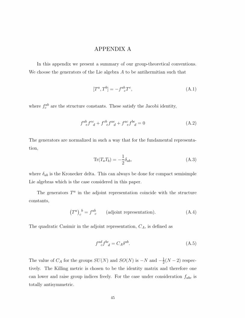
APPENDIX A

In this appendix we present a summary of our group-theoretical conventions.

We choose the generators of the Lie algebra A to be antihermitian such that

[T a, T b] = −fabcT

c, (A.1)

where fabc are the structure constants. These satisfy the Jacobi identity,

fabef

ecd + f cb

efae

d + facef

bed = 0 (A.2)

The generators are normalized in such a way that for the fundamental representa-

tion,

Tr(TaTb) = −1

2δab, (A.3)

where δab is the Kronecker delta. This can always be done for compact semisimple

Lie algebras which is the case considered in this paper.

The generators T a in the adjoint representation coincide with the structure

constants,

(

T a)

cb = fab

c (adjoint representation). (A.4)

The quadratic Casimir in the adjoint representation, CA, is defined as

fadcf

bcd = CAδab. (A.5)

The value of CA for the groups SU(N) and SO(N) is −N and −12(N − 2) respec-

tively. The Killing metric is chosen to be the identity matrix and therefore one

can lower and raise group indices freely. For the case under consideration fabc is

totally antisymmetric.

45

The convention chosen in (A.1) seems unusual but it is the most convenient

when the Wilson line is defined as in (2.13). If we had chosen ifabc instead of

−fabc, the exponential of the Wilson line would have had ig instead of g. Our

convention also introduces a −1 in the vertex (see Fig. 1).

In the rest of this appendix we will describe how Casimirs are evaluated. For the

fundamental representation they are computed by means of an algorithm presented

in [58,59]. The evaluation procedure is simple. We think of the Casimir as a

Feynman diagram, and introduce Feynman diagrammatic notation to replace the

algebraic expressions. The first step is to get rid of the structure constants by

means of the commutation relations i.e., every factor like fabcTc is substituted

by [Tb, Ta]. Once this has been done the expression to be evaluated is a linear

combination of traces of products of generators, with all their indices contracted.

For example in the calculation of C5 we get, among others, the following trace:

Tr(

TaTbTcTdTbTeTdTaTeTc

)

. (A.6)

In general, generators with the same index are not multiplied. If we write the

matrix elements explicitly we can put together the pairs of generators with the

same index, and therefore the quantities we are led to evaluate are of the form,

(

T a) j

i

(

T a) l

k. (A.7)

These group-theoretical objects are called projection operators. They are explicitly

known for every classical Lie group except E8 [58,59]. In the case of SU(N) the

projection operators are:

(

T a) j

i

(

T a) l

k= −1

2

(

δ li δ j

k − 1

Nδ ji δ l

k

)

, (A.8)

and in the case of SO(N),

(

T a) j

i

(

T a) l

k= −1

4

(

δ jk δ l

i − δjlδik

)

. (A.9)

Similar identities can be read from [58] for other groups. This solves the problem

of calculating the Casimirs in the fundamental representation of these groups.

46

Higher representations can be introduced as properly symmetrized products

of fundamental representations. These products span the representation ring of

any compact Lie group. Extensions of (A.8) and (A.9) can be found, which would

enable us to evaluate the analog of (A.7) in these more involved cases. Nevertheless

in the case of SU(2) in representation j nothing of this is needed since its rank

is 1 and therefore all Casimirs are linear combinations of powers of the quadratic

Casimir j(j +1). The key identity is the product of two structure constants (which

will be denoted by εijm) with only one index contracted,

εijmεmkl = δikδjl − δilδjk. (A.10)

Clearly this well-known identity simplifies the calculation of Casimirs in the case

of SU(2). Any Casimir gets reduced to the quadratic Casimir in the corresponding

representation.

Using these rules we have computed all the Casimirs up to order six which have

been used in this paper. These correspond to the fundamental representations of

SU(N) and SO(N), and to an arbitrary spin j representation of SU(2). Their

values are contained in the following list:

SU(N)f : C2 = − 1

2N(N2 − 1)

C3 = − 1

4(N2 − 1)

C4 =1

16(N2 − 1)(N2 + 2)

C5 =1

32N(N2 − 1)(N2 + 1)

C16 =

1

64(N2 − 1)(N4 + N2 + 2)

C26 =

1

64(N2 − 1)(3N2 − 2)

(A.11)

47

SO(N)f : C2 = − 1

4(N − 1)

C3 = − 1

16(N − 1)(N − 2)

C4 =1

256(N − 1)(N − 2)(N2 − 5N + 10)

C5 =1

1024(N − 1)(N − 2)(N3 − 7N2 + 17N − 10)

C16 =

1

4096(N − 1)(N − 2)(N2 − 7N + 14)(N2 − 2N + 3)

C26 =

1

4096(N − 1)(N − 2)(N − 3)(7N − 18)

(A.12)

SU(2)j : C2 = − j(j + 1)

C3 = − j(j + 1)

C4 =2j2(j + 1)2

C5 =3j2(j + 1)2 − j(j + 1)

C16 =2j3(j + 1)3 + 3j2(j + 1)2 − 2j(j + 1)

C26 = − 2j3(j + 1)3 + 5j2(j + 1)2 − 2j(j + 1)

(A.13)

48

APPENDIX B

In this appendix we present some elementary facts about semisimple Lie al-

gebras relevant to the analysis of group factors in the perturbative expansion.

Consider the part of a diagram depicted on the left of Fig. 13. It is possible

to reduce its group factor by means of the totally antisymmetry of the structure

constants fabc at the cost of introducing CA:

fabcTbTc =1

2fabc

[

Tb, Tc

]

=1

2fabcfcbdTd =

1

2CATa. (B.1)

Actually, the Casimir CA can be written in terms of C2 and C3, which is the

expression that we will use wherever a “fishtail” appears:

C3 = − 1

d(R)fabcTr(TaTbTc) = − 1

2d(R)CATr(TaTa) = −1

2CAC2 ⇒ CA = −2C3

C2.

(B.2)

There is a point which may be worth commenting. For an arbitrary semisimple

Lie algebra A = ⊕nk=1Ak in an arbitrary representation, the Wilson line can be

imagined as consisting of n Wilson lines each one corresponding to one of the

simple Lie algebras Ak in its respective representation. Therefore, a connected

(sub)diagram can be regarded as a sum of similar subdiagrams where in each term

the legs are attached to a component of the Wilson line and the sum runs over

all these components. As a consequence one cannot identify the group factors of

diagrams like those in Fig. 14 due to crossed terms in the product of the group

factors of the subdiagrams. If the Lie algebra were simple their group factor would

be the same due to the uniqueness of the Wilson line and to the reduction of the

fishtails.

We call a subdiagram “separated” if its endpoints do not enclose any endpoints

belonging to another subdiagram. For example, the diagrams displayed in Fig. 14

include only separated subdiagrams. In these cases the group factor is a product

of the group factors of the subdiagrams.

49

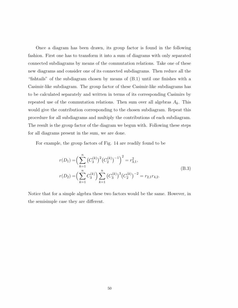
Once a diagram has been drawn, its group factor is found in the following

fashion. First one has to transform it into a sum of diagrams with only separated

connected subdiagrams by means of the commutation relations. Take one of these

new diagrams and consider one of its connected subdiagrams. Then reduce all the

“fishtails” of the subdiagram chosen by means of (B.1) until one finishes with a

Casimir-like subdiagram. The group factor of these Casimir-like subdiagrams has

to be calculated separately and written in terms of its corresponding Casimirs by

repeated use of the commutation relations. Then sum over all algebras Ak. This

would give the contribution corresponding to the chosen subdiagram. Repeat this

procedure for all subdiagrams and multiply the contributions of each subdiagram.

The result is the group factor of the diagram we begun with. Following these steps

for all diagrams present in the sum, we are done.

For example, the group factors of Fig. 14 are readily found to be

r(D1) =(

n∑

k=1

(

C(k)3

)2(C

(k)2

)−1)2

= r23,1,

r(D2) =(

n∑

k=1

C(k)3

)

n∑

k=1

(

C(k)3

)3(C

(k)2

)−2= r2,1r4,2.

(B.3)

Notice that for a simple algebra these two factors would be the same. However, in

the semisimple case they are different.

50

APPENDIX C

In this appendix we list the polynomial knot invariants which have been used in

this paper to compute the numerical knot invariants up to order six for prime knots

up to six crossings. Knot polynomials for the case of SU(2) in a representation of

spin j are collected from [18]. They are:

01 : Vj =1,

31 : Vj =1

[2j + 1]

2j∑

l=0

[2l + 1](−1)2j−lq−3(2j(2j+2)−l(l+1))/2,

41 : Vj =1

[2j + 1]

2j∑

l,k=0

√

[2l + 1][2k + 1]aklql(l+1)−k(k+1),

51 : Vj =1

[2j + 1]

2j∑

l=0

[2l + 1](−1)2j−lq−5(2j(2j+2)−l(l+1))/2,

52 : Vj =1

[2j + 1]

2j∑

l,k=0

√

[2l + 1][2k + 1]akl(−1)kq2j(2j+2)−l(l+1)+3k(k+1)/2,

61 : Vj =1

[2j + 1]

2j∑

l,k=0

√

[2l + 1][2k + 1]alkql(l+1)−2k(k+1),

62 : Vj =1

[2j + 1]

2j∑

i,l,k=0

√

[2i + 1][2k + 1]alialk(−1)2j−l−k

q−3(2j(2j+2)−k(k+1))/2−l(l+1)/2+i(i+1),

63 : Vj =1

[2j + 1]

2j∑

r,s,l,k=0

√

[2s + 1][2k + 1]aklalrars(−1)l+r

q−k(k+1)+s(s+1)+l(l+1)/2−r(r+1)/2,(C.1)

where,

[m] =qm/2 − q−m/2

q1/2 − q−1/2, (C.2)

is a q-number,

[m]! = [m][m − 1][m − 2] . . . [2][1], (C.3)

51

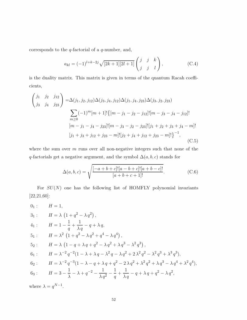
corresponds to the q-factorial of a q-number, and,

akl = (−1)l+k−2j√

[2k + 1][2l + 1]

(

j j k

j j l

)

, (C.4)

is the duality matrix. This matrix is given in terms of the quantum Racah coeffi-

cients,(

j1 j2 j12

j3 j4 j23

)

=∆(j1, j2, j12)∆(j3, j4, j12)∆(j1, j4, j23)∆(j3, j2, j23)

∑

m≥0

(−1)m[m + 1]!{

[m − j1 − j2 − j12]![m − j3 − j4 − j12]!

[m − j1 − j4 − j23]![m − j3 − j2 − j23]![j1 + j2 + j3 + j4 − m]!

[j1 + j3 + j12 + j23 − m]![j2 + j4 + j12 + j23 − m]!}−1

,(C.5)

where the sum over m runs over all non-negative integers such that none of the

q-factorials get a negative argument, and the symbol ∆(a, b, c) stands for

∆(a, b, c) =

√

[−a + b + c]![a − b + c]![a + b − c]!

[a + b + c + 1]!. (C.6)

For SU(N) one has the following list of HOMFLY polynomial invariants

[22,21,60]:

01 : H = 1,

31 : H = λ(

1 + q2 − λ q2)

,

41 : H = 1 − 1

q+

1

λ q− q + λ q,

51 : H = λ2(

1 + q2 − λ q2 + q4 − λ q4)

,

52 : H = λ(

1 − q + λ q + q2 − λ q2 + λ q3 − λ2 q3)

,

61 : H = λ−2 q−2(1 − λ + λ q − λ2 q − λ q2 + 2 λ2 q2 − λ2 q3 + λ3 q3),

62 : H = λ−2 q−3(1 − λ − q + λ q + q2 − 2 λ q2 + λ2 q2 + λ q3 − λ q4 + λ2 q4),

63 : H = 3 − 1

λ− λ + q−2 − 1

λ q2− 1

q+

1

λ q− q + λ q + q2 − λ q2,

where λ = qN−1.

52

Finally, for the Kauffman polynomial invariants [23,60]:

31 : R = 2α2 − α4 +(

−α3 + α5)

z +(

α2 − α4)

z2

41 : R = −1 + α−2 + α2 +

(

1

α− α

)

z +(

−2 + α−2 + α2)

z2 +

(

1

α− α

)

z3

51 : R = 3α4 − 2α6 +(

−2α5 + α7 + α9)

z +(

4α4 − 3α6 − α8)

z2 +(

−α5 + α7)

z3

+(

α4 − α6)

z4

52 : R = α2 + α4 − α6 +(

−2α5 + 2α7)

z +(

α2 + α4 − 2α6)

z2 +(

α3 − 2α5 + α7)

z3

+(

α4 − α6)

z4

61 : R = α−4 − α−2 + α2 +

(

2

α3− 2

α

)

z +

(

3

α4− 4

α2+ α2

)

z2 +

(

3

α3− 2

α− α

)

z3

+

(

1 + α−4 − 2

α2

)

z4 +

(

α−3 − 1

α

)

z5

62 : R = 2 + α−4 − 2

α2+(

α−5 − α−3)

z +

(

3 + α−6 +2

α4− 6

α2

)

z2 +

(

2

α5− 2

α

)

z3

+

(

1 +2

α4− 3

α2

)

z4 +

(

α−3 − 1

α

)

z5

63 : R = 3 − α−2 − α2 +

(

−α−3 +2

α− 2α + α3

)

z +

(

6 − 3

α2− 3α2

)

z2

+

(

−α−3 +1

α− α + α3

)

z3 +

(

4 − 2

α2− 2α2

)

z4 +

(

− 1

α+ α

)

z5

where z = q14 − q−

14 and α = q

N−14 . These invariant polynomials, as well as the

rest of the invariants of this appendix, are given in the standard framing.

53

REFERENCES

1. E. Witten, Comm. Math. Phys. 121(1989), 351

2. M. Bos and V.P. Nair, Phys. Lett. B223(1989), 61, Int. J. Mod.

Phys. A5(1990), 959

3. H. Murayama, “Explicit Quantization of the Chern-Simons Action”, Univer-

sity of Tokyo preprint, UT-542, March 1989

4. J.M.F. Labastida and A.V. Ramallo, Phys. Lett. B227(1989), 92, Phys.

Lett. B228(1989), 214

5. S. Elitzur, G. Moore, A. Schwimmer and N. Seiberg, Nucl.

Phys. B326(1989), 108

6. J. Frohlich and C. King, Comm. Math. Phys. 126(1989), 167

7. G.V. Dunne, R. Jackiw, and C.A. Trugenberger, Ann. Phys. 194(1989), 197

8. S. Axelrod, S. Della Pietra and E. Witten, J. Diff. Geom. 33 (1991) 787

9. J.M.F. Labastida, P.M. Llatas and A.V. Ramallo, Nucl. Phys. B348(1991),

651

10. K. Gawedzki and A. Kupiainen, Comm. Math. Phys. 135(1991), 531

11. E. Witten, Nucl. Phys. B322(1989), 629

12. S.P. Martin, Nucl. Phys. B338(1990), 244

13. J.M.F. Labastida and M. Marino, Santiago preprint, hep-th/9402093, Febru-

ary 1994

14. J.M. Isidro, J.M.F. Labastida and A.V. Ramallo, Nucl. Phys. B398(1993),

187

15. K. Yamagishi, M.-L. Ge and Y.-S. Wu, Lett. Math. Phys. 19(1990), 15

16. S. Mukhi, “Skein Relations and Braiding in Topological Gauge Theory”,

Tata preprint, TIFR/TH/98-39, June 1989

54

17. J.H. Horne, Nucl. Phys. B334(1990), 669

18. R.K. Kaul, T.R. Govindarajan, Nucl. Phys. B380(1992), 293

19. R.K. Kaul and T.R. Govindarajan, Nucl. Phys. B393(1993), 392, Nucl.

Phys. B402(1993), 548

20. V.F.R. Jones, Bull. AMS 12(1985), 103

21. V.F.R. Jones, Ann. of Math. 126 (1987), 335

22. P. Freyd, D. Yetter, J. Hoste, W.B.R. Lickorish, K. Millet and A. Ocneanu,

Bull. AMS 12(1985), 239

23. L.H. Kauffman, Trans. Am. Math. Soc. 318(1990), 417

24. Y. Akutsu and M. Wadati, J. Phys. Soc. Jap. 56(1987), 839;, J. Phys. Soc.

Jap. 56(1987), 3039 Y. Akutsu, T. Deguchi and M. Wadati, J. Phys. Soc.

Jap. 56(1987), 3464;, J. Phys. Soc. Jap. 57(1988), 757; for a review see M.

Wadati, T. Deguchi and Y. Akutsu, Phys. Rep. 180 (1989) 247

25. R.D. Prisarski and S. Rao, Phys. Rev. D22(1985), 208

26. E. Guadagnini, M. Martellini and M. Mintchev, Phys. Lett. B227(1989),

111, Phys. Lett. B228(1989), 489

27. E. Guadagnini, M. Martellini and M. Mintchev, Nucl. Phys. B330(1990),

575

28. L. Alvarez-Gaume, J.M.F. Labastida, and A.V. Ramallo, Nucl.

Phys. B334(1990), 103, Nucl. Phys. B (Proc. Suppl.) 18B (1990) 1

29. D. Birmingham, M. Rakowski and G. Thompson, Nucl. Phys. B234(1990),

83

30. F. Delduc, F. Gieres and S.P. Sorella, Phys. Lett. B225(1989), 367

31. P.H. Damgaard and V.O. Rivelles, Phys. Lett. B245(1989), 48

32. C.P. Martın, Phys. Lett. B241(1990), 513

33. M. Asorey and F. Falceto, Phys. Lett. B241(1990), 31

55

34. A. Blasi and R. Collina, Nucl. Phys. B345(1990), 472

35. F. Delduc, C. Lucchesi, O. Piguet and S.P. Sorella, Nucl. Phys. B346(1990),

513

36. D. Daniel and N. Dorey, Phys. Lett. B246(1990), 82

37. N. Dorey, Phys. Lett. B246(1990), 87

38. C.P. Martın, Phys. Lett. B263(1991), 69

39. G. Giavarini, C.P. Martın and F. Ruiz Ruiz, Nucl. Phys. B381(1992), 222

40. D. Bar-Natan and E. Witten, Comm. Math. Phys. 141(1991), 423

41. D. Bar-Natan, “Perturbative aspects of Chern-Simons topological quantum

field theory”, Ph.D. thesis, Princeton Univ., June 1991, Dept. of Mathematics

42. S. Axelrod and I.M. Singer, MIT preprint, October 1991

43. M. Alvarez and J.M.F. Labastida, Nucl. Phys. B395(1993), 198

44. V.A. Vassiliev, “Cohomology of knot spaces” in Theory of Singularities and

its applications, (V.I. Arnold, ed.), Amer. Math. Soc., Providence, RI, 1990,

23

45. V.A. Vassiliev, “Topology of complements to discriminants and loop spaces”

in Theory of Singularities and its applications, (V.I. Arnold, ed.), Amer.

Math. Soc., Providence, RI, 1990, 23

46. V.A. Vassiliev, “Complements of discriminants of smooth maps: topology

and applications”, Translations of Mathematical Monographs, vol. 98, AMS,

1992

47. D. Bar-Natan, “Weights of Feynman diagrams and the Vassiliev knot invari-

ants”, preprint, 1991

48. J.S. Birman and X.S. Lin, Invent. Math. 111(1993), 225

49. X.S. Lin, Vertex models, quantum groups and Vassiliev knot invariants,

Columbia University preprint, 1991

56

50. E. Witten, Nucl. Phys. B322(1989), 629

51. C. Itzykson and J.B. Zuber, Quantum Field Theory, McGraw-Hill, 1980

52. L.H. Kauffman, Topology 20(1981), 101

53. J.S. Birman, Bull. AMS 28(1993), 253

54. M. Kontsevich, “Graphs, homotopical algebra and low-dimensional topol-

ogy”, preprint, 1992

55. J. Mateos, “Ghosts, knots and Kontsevich integrals”, DAMTP/93-05

preprint, 1993

56. D. Bar-Natan, “On the Vassiliev knot invariants”, Harvard University

preprint, 1993

57. D. Rolfsen, Knots and links, 1976, Berkeley, Calif.: Publish or Perish Press

58. P. Cvitanovic, Group Theory, Nordita Classics Illustrated, 1984

59. P. Cvitanovic, Phys. Rev. D14(1976), 1536

60. F.Y. Wu, Rev. Mod. Phys. 64(1992), 1099

57