arX

iv:g

r-qc

/960

8033

v1 1

4 A

ug 1

996

Lattice knot theory and quantum gravity in the loop representation

Hugo Fort, Rodolfo GambiniInstituto de Fısica, Facultad de Ciencias,

Tristan Narvaja 1674, Montevideo, Uruguay

Jorge PullinCenter for Gravitational Physics and Geometry, Physics Department,

The Pennsylvania State University, 104 Davey Lab, University Park, PA 16802

We present an implementation of the loop representation of quantum gravity on a square lattice.Instead of starting from a classical lattice theory, quantizing and introducing loops, we proceedbackwards, setting up constraints in the lattice loop representation and showing that they haveappropriate (singular) continuum limits and algebras. The diffeomorphism constraint reproducesthe classical algebra in the continuum and has as solutions lattice analogues of usual knot invariants.We discuss some of the invariants stemming from Chern–Simons theory in the lattice context,including the issue of framing. We also present a regularization of the Hamiltonian constraint.We show that two knot invariants from Chern–Simons theory are annihilated by the Hamiltonianconstraint through the use of their skein relations, including intersections. We also discuss the issueof intersections with kinks. This paper is the first step towards setting up the loop representationin a rigorous, computable setting.

gr-qc/9608033

CGPG-96/8-1

ESI-368

I. INTRODUCTION

The use of lattice techniques has proved very fruitful in gauge theories. This is mainly due to two reasons: latticesprovide a regularization procedure compatible with gauge invariance and they allow to put the theory on a computerand to calculate observable quantities. Based on these successes one may be tempted to apply these techniques toquantum gravity. There the situation is more problematic. Lattices introduce preferred directions in spacetime andtherefore break the gauge symmetry of the theory, diffeomorphism invariance. If one studies a canonical formulationof quantum gravity on the lattice this last fact manifests itself in the non-closure of the algebra of constraints.

The introduction of the Ashtekar new variables, in terms of which canonical general relativity resembles a Yang-Mills theory revived the interest in studying a lattice formulation of the theory [1–3]. The new variables allow for amuch cleaner formulation, quite resemblant to that of Kogut and Susskind of gauge theories. However, it does littleto attack the fundamental problem we mentioned in the first paragraph. The lattice formulation still has the problemof the closure of the constraints. The new variable formulation has also allowed to obtain several formal results inthe continuum connecting knot theory with the space of solutions of the Wheeler-DeWitt equation in loop space.This adds an extra motivation for a lattice formulation, since in the lattice context these results could be rigorouslychecked and many of the regularization ambiguities present in the continuum could be settled.

It is not surprising that the lattice counterparts of diffeomorphisms do not close an algebra. A lattice diffeomorphismis a finite transformation. Finite transformations do not structure themselves naturally into algebras but into groups.One cannot introduce an arbitrary parameter that measures “how much” the diffeomorphism shifts quantities alonga vector field. One is only allowed to move things in the fixed amounts permitted by the lattice spacing. It is onlyin the limit of zero lattice spacing, where the constraints represent infinitesimal generators, that one can recoveran algebra structure. The question is: does that algebra structure correspond to the classical constraint algebra ofgeneral relativity? In general it will not.

In this paper we present a lattice formulation of quantum gravity in the loop representation constructed in such away that from the beginning we have good hopes that the diffeomorphism algebra will close in the limit when the latticespacing goes to zero. The strategy will be the following: in the continuum theory the solutions to the diffeomorphismconstraint in the loop representation are given by knot invariants. We will introduce a set of constraints in the latticesuch that their solution space is a lattice generalization of the notion of knot invariants. This means that the solutions,in the limit when the lattice spacing goes to zero, are usual knot invariants. As a consequence the constraints areforced to become the continuum diffeomorphism constraints and close the appropriate algebra. Roughly speaking,if this were not the case they could not have the same solution space as the usual continuum constraints. We willcheck explicitly the closure in the continuum limit. Although this has already been achieved for other proposals ofdiffeomorphism contraints on the lattice [2] the main advantage of our proposal is that our constraints not only close

1

the appropriate algebra in the continuum limit but also admit as solutions objects that reduce in that limit to usualknot invariants, including the invariants from Chern–Simons theory

We will also introduce a Hamiltonian constraint in the space of lattice loops and show that it has the correctcontinuum limit. It remains to be shown if it satisfies the correct algebra relations with the diffeomorphism constraintin the continuum limit.

The main purpose of this paper, however, is to explore how to implement the diffeomorphism symmetry and theidea of knot invariants in the lattice and its relationship to quantum gravity, both at a kinematical and dynamicallevel. We will consider explicit definitions for knot invariants and polynomials, that are the lattice counterpart offormal states of quantum gravity in the continuum formulation. In particular we will introduce the idea of linkingnumber, self-linking number and invariants associated with the Alexander-Conway polynomial. We will also discussthe construction in the lattice of a polynomial related to the Kauffman bracket of the continuum and analyze the issueof the transform into the loop representation of the Chern-Simons state and its relation with the framing ambiguity.We will notice that regular isotopic invariants (invariants of framed loops) are not annihilated by the diffeomorphismconstraint in the lattice. These results allow to put on a rigorous setting many results that were only formally availablein the continuum.

Moreover, we will introduce a Hamiltonian constraint in the lattice whose action on knot invariants can be char-acterized as a set of skein relations in knot space. This allows us to show rigorously that lattice knot invariantsare annihilated by the Hamiltonian constraint, again confirming formal results in the continuum. We also point outdifferences in the details with the continuum results.

Our approach departs in an important way from previous lattice attempts [1–3]: we will work directly in the looprepresentation. There is a good reason for doing this. When one discretizes a theory there are many ambiguitiesthat have to be faced. There are many discretized version of a given continuum theory. If one’s objective is toconstruct a loop representation it is better to discretize at the level of loops than to try to discretize a theory interms of connections and then build a loop representation. We will also start from a non-diffeomorphism formulationat a kinematical level, since it is only in this context that one can study the action of the Hamiltonian constraint ofquantum gravity, which is not diffeomorphism invariant. Moreover it is the only framework in which one can addressthe issue of regular isotopy invariants, which, strictly speaking, are not diffeomorphism invariant. We will then goto a representation that is based on diffeomorphism invariant functions and capture the action of the Hamiltonianconstraint and interpret it as skein relations in that space. We end with a discussion of further possibilities of thisapproach.

II. LATTICE LOOP REPRESENTATION: THE DIFFEOMORPHISM CONSTRAINT

A. The group of loops on the lattice

Consider a three dimensional manifold with a given topology, say S3 and a coordinate patch covering a local sectionof it. We set up a cubic lattice in this coordinate system (this is for simplicity only, none of the arguments we willgive depends on the lattice being square, only on having the same topology as a square lattice). The position of thesites are labeled with latin letters (m, n, ...) where m = (m1,m2,m3) with mi integers, and the links emerging froma given site are labeled by uµ with µ = (−3,−2, . . . , 3), and u±1 = (±1, 0, 0). The typical coordinate lattice spacingwill be denoted by a.

Let us now introduce loops with origin n0. A closed curve is given by a finite chain of vectors

(u1, ....uN ) with

N∑

i=1

ui = 0 (1)

starting at n0. In this paper we will use the word loop in a precise way, analogous to the one that some authors usein the continuum. This notion refers to the fact that there is more information in a closed curve than that neededto compute the holonomy of a connection around the curve. Therefore there are several closed curves that yield thesame holonomy. The equivalence class of such curves is to what we will refer to as loops. In order to define loopson the lattice, we now introduce a reduction process. We define R(u1, ....uN ) as the chain obtained by elimination ofopposite successive vectors

(...uiα, u

i+1µ , ui+2

−µ , ui+3β ...) → (...ui

α, ui+1β ...). (2)

2

Once a couple of vectors is removed,new collinear opposite vectors may appear and must be eliminated. The processis repeated until one gets an irreducible chain. One can show that the reduction process is independent of the orderin which the vectors are removed. A loop γ is an irreducible closed chain of vectors starting at n0. There is a naturalproduct law in loop space. The product of γ1 and γ2 is the reduced composition of their irreducible chains and one canshow that loops form a group [4]. The inverse of γ1 is γ1 = (−uN , ....−u1). We will consider a quantum representationof gravity in which wavefunctions are functions of the group of loops on the lattice Ψ(γ).

Loop representations require considering loops with intersections. Therefore one is interested in intersecting loopson the lattice. We define the intersection class of a loop by assigning a number to each intersection and making a listobtained by traversing the loop and listing the numbers of the successive intersections traversed. Two loops will belongto the same intersection class if the lists of numbers are the same. The concept of intersection class will help definelater the transformations that behave like diffeomorphisms on the lattice. Intersecting loops behave as a “boundary”between different knot classes of non-intersecting loops. We will therefore require that the transformations do not“cross the boundary” by requesting that they do not change the intersection class of the loops. Any deformation ofthe loop that does not make it cut itself preserves the intersection class. Wavefunctions in the loop representation arecyclic functions of loops and therefore we will identify loops belonging to the same intersection class through cyclicrearrangements.

B. The diffeomorphism constraint: continuum limit

We now proceed to write a generator of deformations on the lattice, which in the continuum limit will yield thediffeomorphism constraint. We define an operator dµ(n) that deforms the loop at the point n of the lattice as shownin figure 1. For example, the action of the operator on a chain,

γ = (...ui(n), ui+1(n)...uj(n), uj+1(n)...uk(n), uk+1(n)...) (3)

is,

γD ≡ dµ(n)γ ≡ R(...uµ, ui(n), ui+1(n), u−µ...uµ, u

j(n), uj+1(n), u−µ (4)

...uµ, uk(n), uk+1(n), u−µ...).

FIG. 1. The action of the deformation operator on a lattice loop at a regular point and at an intersection.

In the above example we have a loop that goes three times through the same point. If the point n does not lie onthe loop considered the deformation operator leaves the loop invariant. The action of the deformation operator is toadd two plaquettes one before and one after the point at which it acts along the line of the loop. If the action takesplace at an intersection, as in the example shown, the deformation adds two plaquettes along each line going throughthe intersection.

We now define an admissible deformation as a deformation that does not change the intersection type of the loop.Admissible deformations are constructed with the operator dµ(n) but defining its action to be unity in the casein which the loop would change its intersection class as a consequence of the deformation. Typical examples ofdeformations that change the intersection class arise when one has parallel lines separated by one lattice spacing inthe loop and one deforms in a transverse direction. These deformations are set to unity.

We now consider a quantum representation formed by wavefunctions Ψ(γ) of loops on the lattice. One can thereforeintroduce an operator which implements the admissible deformations of the loops Dµ(n)Ψ(γ) = Ψ(dµ(n)γ) and anassociated operator,

3

Cµ(n)Ψ(γ) ≡(1 + Pµ(n))

4(Dµ(n)Ψ(γ) −D−µ(n)Ψ(γ)) . (5)

where the weight factor Pµ(n) counts the number of non-admissible deformations that the displacements would create.If both displacements are admissible the overall factor is 1/4, if one is non-admissible, it is 1/2. This factor is neededto ensure consistency of the algebra of constraints.

We will show that this operator, when acting on a holonomy on the lattice, produces the usual diffeomorphismconstraint of the Ashtekar formulation in the continuum limit. We will take the continuum limit in a precise way: wewill assume that loops are left of a fixed length and the lattice is refined. As a consequence of this, loops will neverhave two parallel sections separated by only one plaquette. Due to this, for any given calculation we only need toconsider three different kinds of points in the loop: regular points, corners and intersections. The intersections canhave corners or go “straight through”.

Before going into the explicit computations it is worthwhile analyzing up to what extent can one recover dif-feomorphisms from a lattice construction. After all, all deformations on the lattice are discrete and are thereforehomeomorphisms. It is clear that at regular points of the loop there is no problem, the addition of plaquettes be-comes in the limit the infinitesimal generator of deformations, as we shall see. The situation is more complicatedat intersections. Deformations that do not occur at the intersection, but at points adjacent to it can change thenature of the intersection. For instance, an intersection that goes “straight through” can be made to have a kink bydeforming at an adjacent point. In the continuum, a diffeomorphism cannot change straight lines into lines with kinks,therefore the above kind of deformations must be forbidden if one wants the lattice transformations to correspondto diffeomorphisms in the continuum. Because of the way we are taking the continuum limit this situation does notoccur, since all points of the loop are either at an intersection or far away from it. We will see, however, that thisproblem resurfaces when one wants to compute the diffeomorphism algebra, and we will discuss it there.

In order to see that the above operator corresponds in the continuum to the generator of diffeomorphism we considera holonomy along a lattice loop T 0(γ) ≡ Tr[

∏

l∈γ U(l)] where U(l) = exp aAb(n), a is the lattice spacing and Ab(n)is the Ashtekar connection at the site n. Then,

Cµ0(n)T 0(γ) =

(1 + Pµ(n))

4[T 0(dµγ) − T 0(d−µγ)]. (6)

In the limit a → 0 while the loop remains finite, this action is always a local deformation (in the sense that thereare no lines of the loop in a neighborhood of each other). Assuming the connections are smooth, we get,

Cµ(n)T 0(γ) = 12

(

a2Nn(γ)Tr[Fab(n)U(γ)]uaµu

bν(n) (7)

+a2Nn(γ)Tr[Fab(n)U(γ)]uaµu

bν′(n)

)

where ν and ν′ represent the links adjacent to the site n on the loop and Nn(γ) is a function that is 1 if n is on theloop γ and zero otherwise, so Nn(γ) =

∑

n′∈γ δn,n′ where δn,n′ is a Kronecker delta.But

lima→0

Nn(γ)a(uaν + ua

ν′)

2a3=

∫

γ

dyaδ(x− y) ≡ Xa(x, γ) (8)

where x = lima→0 na, x = lima→0 n′a and we have used that lima→0δna,n′a/a

3 = δ(x− y). Therefore

lima→0

1/a4Cµ(n)T 0(γ) = uaµX

b(x, γ)∆ab(γx)T 0(γ) = (9)

uaµ

∫

γ

dybδ(x− y)∆ab(γy)T 0(γ) = ua

µFiab(x)

δ

δAib

T 0(γ) = uaµCaT

0(γ) (10)

which is the explicit form of the vector constraint Cb = ˆEa

i Fiab in the Ashtekar formulation.

This procedure is valid for any regular point of the loop or corner. A similar procedure may be followed for a siteincluding intersections or corners. It can be straightforwardly verified that the vector constraint is also recovered inthose cases.

4

C. The diffeomorphism constraint: constraint algebra

In order to have a consistent quantum theory, one has to show that the quantum constraint algebra reproduces toleading order in h the classical one. In a lattice theory, the objective is to show that the quantum constraint algebrareproduces the classical one in the continuum limit. Specifically, for the case of diffeomorphisms,

[ lima→0

Cµ(n)

a4, lima→0

Cν(n′)

a4] = lim

a→0

1

a8[Cµ(n), Cν(n′)]. (11)

We will here show that the correct algebra is reproduced in the limit in which the lattice spacing goes to zero. Thisis an important calculation, since it is not obvious that diffeomorphism symmetry can be implemented in a squarelattice framework as we propose here. We will see that there are subtle points in the calculation. We will present theexplicit calculation for a regular point of the loop only in an explicit fashion. Even for that case the calculation isquite involved.

n’

1

2

3

231312

n

n’

n

n=n’-1, n=n’-1.

n’

n

n=n’-1+3.

n’

n

n=n’-1+3.

n’ n

n=n’-1-3

n

n’

n=n’-1-3.

n’

n

n=n’+3.

n’

n

n=n’+3.

n’

n

n’

n

n=n’-3. n=n’-3.

FIG. 2. The action of the first portion of terms in the commutator of two diffeomorphism constraints acting at a regularlattice point.

Let us now consider the algebra of the operators Cµ(n) and Cν(n′) and its continuum limit. As before, we assumethat a refinement of the lattice has taken place with the loop length remaining finite in such a way that any pointof the loop is either in a corner, intersection or regular point. We will only discuss explicitly the case in whichthe commutator is evaluated at a regular point. To simplify the notation, we will consider µ and ν in directionsperpendicular to the loop and we take three coordinate axes 1, 2, 3 with 3 parallel to the loop and the other twoperpendicular. We will compute [C2(n), C1(n

′)]ψ(γ). Let us consider first the term C2(n)C1(n′). In order for it to

be nonvanishing, the point n′ has to be on the loop γ. The first diffeomorphism generates two terms, correspondingto the addition of two plaquettes in the forward 1 direction and backward. The second diffeomorphism will lead tonon-zero commutator if the point n lies in one of the points marked in figure 2 on the deformed loop. There are fivepossible such points along the deformation. At each the action of the second diffeomorphism generates two terms.The resulting ten deformed loops are shown explicitly in the figure 2. There will be ten similar terms resulting fromthe “backwards” action of the first diffeomorphism. To clarify the calculation, let us concentrate on the first pairof terms displayed in figure 2. The infinitesimal deformation of the original loop γ generated by the loop derivativeoperator [9] is represented through the introduction in the holonomy of field strengths Fab(P, p) , depending on a

5

path P and its end point p, contracted with the element of area of the plaquette. To unclutter the notation, when aplaquette in the direction 1 − 2 is added, we will denote this as F12(p) dropping the dependence in the path P (weassume the path goes from the basepoint of the loop to the point of interest). With this notation, the contribution ofthe first two terms of figure 2 is (we are neglecting all the contributions of powers greater than a2),

Nγ(n′){Tr[ (F23(n′ − 1) + F23(n

′ − 1) )U(γ)]

−Tr[ (−F23(n′ − 1) − F23(n

′ − 1) )U(γ)]} (12)

where by −1, −3, etc we denote the point displaced one lattice unit in the corresponding direction, the sign indicatingforward or backward respect to the orientation chose in the trihedron shown in the figure.

We see that the contribution of the plaquettes added by the first diffeomorphism, namely the F ′13s cancel each other

at this order. Taking into account these cancellations, the result of all the terms considered in figure 2 is,

Nγ(n′){δ(n− n′ + 1)Tr[(F23(n′ − 1) + F23(n

′ − 1))U(γ)]

−δ(n− n′ + 1)Tr[(−F23(n′ − 1) − F23(n

′ − 1))U(γ)]

+δ(n− n′ + 1 − 3)Tr[(F23(n′ − 1 + 3) − F12(n

′ − 1 + 3))U(γ)]

−δ(n− n′ + 1 − 3)Tr[(−F23(n′ − 1 + 3) + F12(n

′ − 1 + 3))U(γ)]

+δ(n− n′ + 1 + 3)Tr[(F12(n′ − 1 − 3) + F23(n

′ − 1 − 3))U(γ)]

−δ(n− n′ + 1 + 3)Tr[(−F12(n′ − 1 − 3) − F23(n

′ − 1 − 3))U(γ)]

+δ(n− n′ − 3)Tr[(−F12(n′ + 3) + F23(n

′ + 3))U(γ)]

−δ(n− n′ − 3)Tr[(F12(n′ + 3) − F23(n

′ + 3))U(γ)]

+δ(n− n′ + 3)Tr[(F23(n′ − 3) + F12(n

′ − 3))U(γ)]

−δ(n− n′ + 3)Tr[(−F23(n′ − 3) − F12(n

′ − 3))U(γ)]} (13)

where we have, to make more direct the continuum analysis used the notation of Dirac deltas for what strictly speakingare Kronecker deltas at this stage of the calculation.

We now need to consider the terms from the “backwards” action of the first diffeomorphism constraint. This givesrise to the contributions depicted in figure 3 and are explicitly given by,

Nγ(n′){δ(n− n′ − 1)Tr[(F23(n′ + 1) + F23(n

′ + 1))U(γ)]

−δ(n− n′ − 1)Tr[(−F23(n′ + 1) − F23(n

′ + 1))U(γ)]

+δ(n− n′ − 1 − 3)Tr[(F23(n′ + 1 + 3) + F12(n

′ + 1 + 3))U(γ)]

−δ(n− n′ − 1 − 3)Tr[(−F23(n′ + 1 + 3) − F12(n

′ + 1 + 3))U(γ)]

+δ(n− n′ − 1 + 3)Tr[(−F12(n′ + 1 − 3) + F23(n

′ + 1 − 3))U(γ)]

−δ(n− n′ − 1 + 3)Tr[(F12(n′ + 1 − 3) − F23(n

′ + 1 − 3))U(γ)]

+δ(n− n′ − 3)Tr[(F12(n′ + 3) + F23(n

′ + 3))U(γ)]

−δ(n− n′ − 3)Tr[(−F12(n′ + 3) − F23(n

′ + 3 − 2))U(γ)]

+δ(n− n′ + 3)Tr[(F23(n′ − 3) − F12(n

′ − 3))U(γ)]

−δ(n− n′ + 3)Tr[(−F23(n′ − 3) + F12(n

′ − 3))U(γ)]} (14)

6

1

2

3

231312

FIG. 3. The second portion of the terms of the commutator of two diffeomorphisms at a regular point of the lattice.

The terms in the above two expressions can be combined to form a series of differences of delta’s times F ’s,

4Nγ(n′){∆1[ 2δ(n′ − n)Tr[F23(n′))U(γ)]

+δ(n′ − n− 3)Tr[(F23(n′ + 3)U(γ)]

+δ(n′ − n+ 3)Tr[F23(n′ − 3)U(γ)] ]

+∆3[2δ(n′ − n)Tr[F12(n

′)U(γ)]

+δ(n′ − n− 1)Tr[F12(n′ + 1)U(γ)]

+δ(n′ − n+ 1)Tr[F12(n′ − 1)U(γ)] ]}, (15)

where the differences ∆µ mean evaluate the quantity at n′ and n′ + µ and take the difference. The derivatives of F23

along the direction 1 are formed by the first six terms of (14) and (13) (the term multiplied by 2 comes from the firsttwo lines and the remaining from the next four lines). The last four terms give vanishing contributions for F23. Thederivatives along 3 of F12 are produced in two identical copies by (14) and (13), combining the contribution of eachline with the one two lines below in F12.

To understand this result it is useful to pay attention to the shading in figure 3, since we see that the contributionsto the action of the successive operators is mirrored by the shaded areas of the figure. All the unshaded plaquettescancel each other in the various terms. Only the shaded ones survive. For instance, the 2 − 3 shaded plaquettes tothe front, of which we have two in the first drawing of figure 3, two in the second and one in the third, fourth, fifthand sixth, minus the corresponding terms of figure 2 give rise to the first, second and third terms of equation (15).

Equation (15) can be rewritten as

4Nγ(n′){∆1[ 2δ(n− n′)Tr[F23(n′)U(γ)]

+δ(n− n′ − 3)Tr[F23(n′ + 3)U(γ)]

+δ(n− n′ + 3)Tr[F23(n′ − 3)U(γ)] ]

+∆3[ 2δ(n− n′)Tr[F12(n′)U(γ)]

+δ(n− n′ − 1)Tr[F12(n′ + 1)U(γ)]

+δ(n− n′ + 1)Tr[F23(n′ − 1)U(γ)] ] }. (16)

In order to write the commutator [C2(n), C1(n′)]ψ(γ) we have to subtract to (16) the same expression but interchanging

1 ↔ 2 and n↔ n′. If we now express the Nγ(p) as∑

m∈γ δ(p−m) then we get

[C2(n), C1(n′)] =

1

4

∑

m′∈γ

δ(n′ −m′){∆1[ 2δ(n−m′)Tr[F23(m′)U(γ)]

+δ(n−m′ − 3)Tr[F23(m′ + 3)U(γ)]

+δ(n−m′ + 3)Tr[F23(m′ − 3)U(γ)] ]

7

+∆3[ 2δ(n−m′)Tr[F12(m′)U(γ)]

+δ(n−m′ − 1)Tr[F12(m′ + 1)U(γ)]

+δ(n−m′ + 1)Tr[F23(m′ − 1)U(γ)] ] }

−1

4

∑

m∈γ

δ(n−m){∆1[ 2δ(n′ −m)Tr[F13(m)U(γ)]

+δ(n′ −m− 3)Tr[F13(m+ 3)U(γ)]

+δ(n′ −m+ 3)Tr[F13(m− 3)U(γ)] ]

+∆3[ 2δ(n′ −m)Tr[F21(m)U(γ)]

+δ(n′ −m− 2)Tr[F21(m+ 2)U(γ)]

+δ(n′ −m+ 2)Tr[F21(m− 2)U(γ)] ] } (17)

If we now neglect terms of higher order in the lattice spacing, we can move all the delta’s and F ’s to the samelocations and, taking into account the explicit dependence on the lattice spacing a the equation (17) becomes

[C2(x), C1(y)] = lima→0

[C2(na)

a4,C1(n

′a)

a4] = lim

a→0

1

a6

∑

m∈γ

{ δ(n′ −m)∆1δ(n−m)Tr[F23(m)U(γ)]

−∆2δ(n′ −m)δ(n−m)Tr[F13(m)U(γ)]

+δ(n′ −m)δ(n−m)∆1Tr[F23(m)U(γ)]

+δ(n′ −m)δ(n−m)∆2Tr[F31(m)U(γ)]

+δ(n′ −m)δ(n−m)∆3Tr[F12(m)U(γ)]

+∆3δ(n′ −m)δ(n−m)Tr[F12(m)U(γ)]

+δ(n−m)∆3δ(n′ −m)Tr[F12(m)U(γ)]

+δ(n−m)δ(n′ −m)∆3Tr[F12(m)U(γ)] } (18)

where the power 1/a6 arises from the fact that implicit in all the previous calculations was an a2 power, as wementioned at the beginning. The third, fourth and fifth terms of (18) cancel out by virtue of the Bianchi identity.The sixth, seventh and eighth form a total derivative along the 3-direction.

Recalling that δ(na−ma)/a3 → δ(x− z) and ∆1δ(na−ma)/a4 → ∂1δ(x− z) we arrive to

[C2(x), C1(y)] =

{ ∂1δ(y − x)

∫

γ

dzδ(y − z)Tr[F23(y)U(γ)]

−∂2( δ(x− y) )

∫

γ

dzδ(x− z)Tr[F13(x)U(γ)] }. (19)

The calculation displayed above is true at a regular point of the loop. A similar calculation can be performed atcorners with the same result. A problem arises, however, at intersections. This is related to the issue we discussedbefore of homeomorphisms vs diffeomorphisms. As we pointed out, the operator we introduced generates diffeomor-phisms at regular points of the loop or at intersections or corners. A problem develops if one acts in points that areimmediately adjacent to intersections, since the deformation can change the character of intersections (introducingkinks). One cannot ignore this fact in the commutator algebra. When one acts with two successive diffeomorphismsat an intersection, it is inevitable to consider one of the operators as acting at a point adjacent to the intersectionbefore taking the continuum limit. This leads to changes in the character of the intersection that we do not want toallow. If we did so, we would not recover diffeomorphism in the continuum but homeomorphisms, which can introducekinks in the intersection. If one allows these kind of deformations in the lattice, the calculation of the algebra atintersections goes through with no problem. In the continuum, the only difference between the homeomorphism anddiffeomorphism algebra is given by the nature of the smearing functions of the constraints, so it is not surprising thatwe recover the same algebra. If one restricts the action of the deformations in order to avoid changing the characterof intersections, by defining the action of the operator to be unity if it changes the character of the intersection,the commutator algebra fails at intersections. More precisely, the constraints commute at intersections. Becausethis failure of the constraint algebra occurs only at a zero measure set of points, one can still consider the quantum

8

theory to be satisfactory, since one is smearing the constraints with smooth functions and therefore cannot distinguishthis algebra from one with different values of the commutators at a zero measure set of points. We will adopt thislatter point of view in this paper, since our primary motivation is to implement diffeomorphism symmetry in thecontinuum. This will also have a practical consequence: because homeomorphism invariance is more restrictive thandiffeomorphism invariance we will see that it is considerably easier to find invariants under diffeomorphisms thanunder homeomorphisms.

III. KNOTS ON THE LATTICE

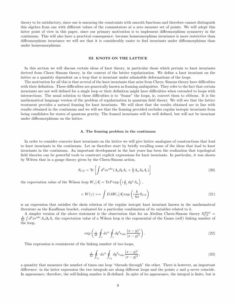
In this section we will discuss certain ideas of knot theory, in particular those which pertain to knot invariantsderived from Chern–Simons theory, in the context of the lattice regularization. We define a knot invariant on thelattice as a quantity dependent on a loop that is invariant under admissible deformations of the loops.

The motivation for all this is that several of the knot invariants that arise from Chern–Simons theory have difficultieswith their definition. These difficulties are generically known as framing ambiguities. They refer to the fact that certaininvariants are not well defined for a single loop or their definition might have difficulties when extended to loops withintersections. The usual solution to these difficulties is to “frame” the loops, ie, convert them to ribbons. It is themathematical language version of the problem of regularization in quantum field theory. We will see that the latticetreatment provides a natural framing for knot invariants. We will show that the results obtained are in line withresults obtained in the continuum and we will see that the framing provided excludes regular isotopic invariants frombeing candidates for states of quantum gravity. The framed invariants will be well defined, but will not be invariantunder diffeomorphisms on the lattice.

A. The framing problem in the continuum

In order to consider concrete knot invariants on the lattice we will give lattice analogues of constructions that leadto knot invariants in the continuum. Let us therefore start by briefly recalling some of the ideas that lead to knotinvariants in the continuum. An important development in the last years has been the realization that topologicalfield theories can be powerful tools to construct explicit expressions for knot invariants. In particular, it was shownby Witten that in a gauge theory given by the Chern-Simons action,

SCS = Tr

[∫

d3xǫabc(Aa∂bAc + 23AaAbAc)

]

(20)

the expectation value of the Wilson loop Wγ [A] = TrP exp(

i∮

γdyaAa

)

,

< W (γ) >=

∫

DAWγ [A] exp

(

ik

8πSCS

)

(21)

is an expression that satisfies the skein relation of the regular isotopic knot invariant known in the mathematicalliterature as the Kauffman bracket, evaluated for a particular combination of its variables related to k.

A simpler version of the above statement is the observation that for an Abelian Chern-Simons theory SAbelCS =

k8π

∫

d3xǫabcAa∂bAc the expectation value of a Wilson loop is the exponential of the Gauss (self) linking number ofthe loop,

exp

(

i2k

∮

γ

dxa

∮

γ

dybǫabc(x− y)c

|x− y|3

)

. (22)

This expression is reminiscent of the linking number of two loops,

14π

∮

γ1

dxa

∮

γ2

dybǫabc(x − y)c

|x− y|3, (23)

a quantity that measures the number of times one loop “threads through” the other. There is however, an importantdifference: in the latter expression the two integrals are along different loops and the points x and y never coincide.In appearance, therefore, the self-linking number is ill-defined. In spite of its appearance, the integral is finite, but is

9

ambiguously defined, its definition requires the introduction of a normal to the loop, which is not a diffeomorphisminvariant concept. This problem is known as the framing ambiguity and it is clearly related to regularization. Supposeone attempts to define the self-linking number by considering the linking number of a loop as the linking number ofthe loop with a “copy” of itself, obtained by displacing the loop an infinitesimal amount. This clearly regularizes theintegral. However, the result depends on how one creates the “copy” of the loop and how it winds around the originalloop. One of the main purposes of this paper will be to show how to address the framing ambiguity in the lattice.We will start by discussing the Abelian case.

The above problem is more acute if the loops have intersections. In that case the integral tha appears in theself-linking number is not even finite. Again, one can in principle solve the problem through a mechanism of framing.An important aspect of the lattice construction will therefore be to provide a precise mechanism for framing knotinvariants with intersections.

Why is one interested in these particular invariants?. There are two reasons. On one hand, because they areconstructed as loop transforms of quantities in terms of connections these invariants automatically satisfy the “Man-delstam constraints” that must be satisfied by wavefunctions of quantum gravity in the loop representation. Thismakes them candidates for quantum states of gravity. Moreover, it has been concretely shown that some of theinvariants that arise due to Chern-Simons theory formally solve the Hamiltonian constraint of quantum gravity in thecontinuum. The lattice framework is an appropriate environment to discuss these solutions in a rigorous setting.

B. Abelian Chern-Simons theory on the lattice

Let us start with the simple case of a U(1) Chern-Simons theory and study its lattice version. Although this is notdirectly connected with quantum gravity we will see that it already contains several ingredients we are interested inand in particular it allows the discussion of the self-linking number, which plays a central role in quantum gravity inthe continuum.

The Chern-Simons invariant can be written naturally in the lattice in terms of a wedge product, as discussed inreferences [6,7]. In order to give more details we need to briefly introduce the differential form calculus on the lattice[8].

A k-form on the lattice is a function associated with a k-dimensional cell Ck in the lattice that is skew-symmetricwith respect to the orientation of the cell. For instance, a zero-form is a scalar field (associated with lattice sites),a one-form is a variable associated with lattice links that changes sign when one changes the orientation of the link.A two-form is a variable associated with a plaquette, with sign determined by the orientation of the plaquette. Theexterior derivative is a map between k and k + 1 forms defined by,

dφ(Ck+1) =∑

C′

K∈∂Ck+1

φ(C′k) (24)

where φ(Cn) is an n-form and the sum is along the cells that form the boundary of Ck+1. For instance, given a oneform A(C1), we can define a two-form F (C2) obtained by summing A along all the links that encircle the plaquetteC2 and which we denote as F = dA.

One can also introduce a co-derivative operator δ which associates a k − 1 form with a k form, through

δφ(Ck−1) =∑

∀Ck/Ck−1∈∂Ck

φ(Ck). (25)

From the above definitions one can see that both operators are nilpotent,

δ2 = 0, d2 = 0, (26)

and in terms of these operators one can define a Laplacian, which maps k-forms to themselves,

∇2 ≡ δd+ dδ. (27)

To conclude these mathematical preliminaries we introduce a notion of inner product on the lattice. The innerproduct of two k-forms is defined by,

< φ,ϕ >=∑

∀Ck

φ(Ck)ϕ(Ck), (28)

10

and this product has the property of “integration by parts”,

< dφ, ϕ >=< φ, δϕ > . (29)

With these elements we are able to introduce the Chern-Simons form through the definition of a wedge productthat associates (in three dimensions) a one-form to each two-form and vice-versa. Given a two-form associated with aplaquette C2, the wedge product defines a one-form associated with a link C1 orthogonal to C2, whose value is givenby the value of the one-form evaluated on C2. Evidently there is an ambiguity in how to define the wedge productsince there are eight links orthogonal to each plaquette. We will see that different definitions of the wedge productwill correspond to different framings in the context of knot invariants. There exist several definitions which all implythe following identities,

#dA = δ#A, (30)

#δA = d#A. (31)

One possible consistent way to define the # operation is to assign to a two-form associated with an orientedplaquette an average of the one-forms associated with each of the eight links perpendicular to the plaquette along itsperimeter. This differs from the definition taken in [7] which assigns only one link, but we will adopt it in this paperbecause it yields a more symmetric framing of the knot invariants.

With the above notation, the Chern-Simons form in the lattice can be written as,

SAbelCS = ik < F,#A > . (32)

This action is gauge invariant under transformations A→ A+ dξ, since the transformation implies

SCS → SCS + ik < F,#dξ >= SCS + ik < F, δ#ξ >= SCS + ik < dF,#ξ >= SCS + ik < d2A,#ξ >= SCS . (33)

One can now proceed to compute the expectation value of a Wilson loop in a Chern-Simons theory on the lattice,

< W (γ) >=

∫

DA exp(

SAbelCS

)

T 0(γ), (34)

which, after a straightforward Gaussian integration yields,

exp

(

−i

2k< #lγ , d∇

−2lγ >

)

(35)

where lγ(C1) is a one-form such that it is one if C1 belongs to the loop γ and zero otherwise. This expression takesinteger values and has a simple interpretation. In order to see this, recall that in S3 (or any simply connected regionof an arbitrary manifold), the one form l satisfies δl = 0 and therefore can be written as a co-derivative of a two formm,

l = δm (36)

and substituting in the expression (34) and using (30) and (27) expression (34) reduces to,

< #mγ , lγ > . (37)

This expression is the particularization to one loop of the linking number on the lattice, which we discuss in detailin the next section and is usually called the self-linking number. We will also return, at the end of it, to the self-linkingnumber.

C. The Gauss linking number in the lattice and self-linkings

The linking number of two loops η and γ on the lattice is given by

N(η, γ) =< #mη, lγ > . (38)

11

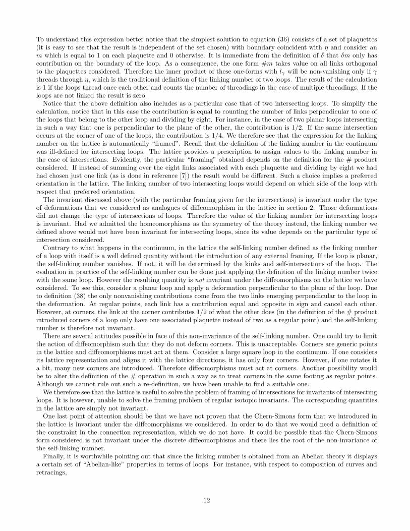
To understand this expression better notice that the simplest solution to equation (36) consists of a set of plaquettes(it is easy to see that the result is independent of the set chosen) with boundary coincident with η and consider anm which is equal to 1 on each plaquette and 0 otherwise. It is immediate from the definition of δ that δm only hascontribution on the boundary of the loop. As a consequence, the one form #m takes value on all links orthogonalto the plaquettes considered. Therefore the inner product of these one-forms with lγ will be non-vanishing only if γthreads through η, which is the traditional definition of the linking number of two loops. The result of the calculationis 1 if the loops thread once each other and counts the number of threadings in the case of multiple threadings. If theloops are not linked the result is zero.

Notice that the above definition also includes as a particular case that of two intersecting loops. To simplify thecalculation, notice that in this case the contribution is equal to counting the number of links perpendicular to one ofthe loops that belong to the other loop and dividing by eight. For instance, in the case of two planar loops intersectingin such a way that one is perpendicular to the plane of the other, the contribution is 1/2. If the same intersectionoccurs at the corner of one of the loops, the contribution is 1/4. We therefore see that the expression for the linkingnumber on the lattice is automatically “framed”. Recall that the definition of the linking number in the continuumwas ill-defined for intersecting loops. The lattice provides a prescription to assign values to the linking number inthe case of intersections. Evidently, the particular “framing” obtained depends on the definition for the # productconsidered. If instead of summing over the eight links associated with each plaquette and dividing by eight we hadhad chosen just one link (as is done in reference [7]) the result would be different. Such a choice implies a preferredorientation in the lattice. The linking number of two intersecting loops would depend on which side of the loop withrespect that preferred orientation.

The invariant discussed above (with the particular framing given for the intersections) is invariant under the typeof deformations that we considered as analogues of diffeomorphism in the lattice in section 2. Those deformationsdid not change the type of intersections of loops. Therefore the value of the linking number for intersecting loopsis invariant. Had we admitted the homeomorphisms as the symmetry of the theory instead, the linking number wedefined above would not have been invariant for intersecting loops, since its value depends on the particular type ofintersection considered.

Contrary to what happens in the continuum, in the lattice the self-linking number defined as the linking numberof a loop with itself is a well defined quantity without the introduction of any external framing. If the loop is planar,the self-linking number vanishes. If not, it will be determined by the kinks and self-intersections of the loop. Theevaluation in practice of the self-linking number can be done just applying the definition of the linking number twicewith the same loop. However the resulting quantity is not invariant under the diffeomorphisms on the lattice we haveconsidered. To see this, consider a planar loop and apply a deformation perpendicular to the plane of the loop. Dueto definition (38) the only nonvanishing contributions come from the two links emerging perpendicular to the loop inthe deformation. At regular points, each link has a contribution equal and opposite in sign and cancel each other.However, at corners, the link at the corner contributes 1/2 of what the other does (in the definition of the # productintroduced corners of a loop only have one associated plaquette instead of two as a regular point) and the self-linkingnumber is therefore not invariant.

There are several attitudes possible in face of this non-invariance of the self-linking number. One could try to limitthe action of diffeomorphism such that they do not deform corners. This is unacceptable. Corners are generic pointsin the lattice and diffeomorphisms must act at them. Consider a large square loop in the continuum. If one considersits lattice representation and aligns it with the lattice directions, it has only four corners. However, if one rotates ita bit, many new corners are introduced. Therefore diffeomorphisms must act at corners. Another possibility wouldbe to alter the definition of the # operation in such a way as to treat corners in the same footing as regular points.Although we cannot rule out such a re-definition, we have been unable to find a suitable one.

We therefore see that the lattice is useful to solve the problem of framing of intersections for invariants of intersectingloops. It is however, unable to solve the framing problem of regular isotopic invariants. The corresponding quantitiesin the lattice are simply not invariant.

One last point of attention should be that we have not proven that the Chern-Simons form that we introduced inthe lattice is invariant under the diffeomorphisms we considered. In order to do that we would need a definition ofthe constraint in the connection representation, which we do not have. It could be possible that the Chern-Simonsform considered is not invariant under the discrete diffeomorphisms and there lies the root of the non-invariance ofthe self-linking number.

Finally, it is worthwhile pointing out that since the linking number is obtained from an Abelian theory it displaysa certain set of “Abelian-like” properties in terms of loops. For instance, with respect to composition of curves andretracings,

12

N(γ1 ◦ γ2, γ3) = N(γ1, γ3) +N(γ2 ◦ γ3) (39)

N(γ, η−1) = −N(γ, η), (40)

these properties will be crucial for the results we will derive in the next section.In the continuum, through the use of variational techniques, skein relations have been provided for the Kauffman

bracket knot polynomial [15]. These results contain as a particular case skein relations for the linking number withintersections. It is worthwhile pointing out that these results agree with the results we presented in the previousparagraphs. The skein relation found states that,

N( ) =1

2(N( ) +N( )) (41)

which implies that the value of the linking number of two loops with an intersection is equal to average of the valuesof the linking number when that intersection is replaced by an upper or an under crossing. In one case the invariantwill be 1 and in the other zero and therefore we recover the lattice result that the linking number of two loops thatare only linked through an intersection is one half. If the intersection had kinks in it, the continuum results containa free parameter. This parameter can be adjusted to agree with the lattice results.

IV. THE HAMILTONIAN CONSTRAINT

A. Definition

Let us now define the action of the Hamiltonian constraint. We will propose an operator largely based on the expe-rience of the continuum [9]. We know the operator is only nonvanishing at points where the loops have intersections.For pedagogical reasons we first write the definition for a concrete simple loop and then we give the general definition.Consider a figure eight loop η as shown in figure 4. The action of the Hamiltonian on the state is given by,

o

o o

o o

η

η1

η2

η3

η4

FIG. 4. The loops that arise in the action of the Hamiltonian on a figure eight loop.

13

H(n)ψ(η) =1

4[ψ(η1) − ψ(η2) + ψ(η3) − ψ(η4)]. (42)

The action of the operator at intersections can be described as deforming the loop along one of the tangents at theintersection and rerouting one of the resulting lobes minus the rerouted deformation in the opposite direction. Thisoperation is carried along for each possible pair of tangents at the intersection. The “lobes” do not need to be singlelobes as depicted here, the situation is the same in multiple intersections, each pair of tangents determines univocallytwo lobes in the loop.

Let us now describe the general definition of the Hamiltonian acting on a loop with possible multiple intersectionsat a point with possible kinks. We start from a generic loop on the lattice described by a chain of links,

γ = (. . . , u−(n), u+(n), . . . , v−(n), v+(n), . . .) (43)

where u−(n), u+(n), . . . are the incoming and outgoing links at the intersection, which we locate at the site n. Theintersection can be multiple, in that case one has to choose pairs of lines that go through it and add a contributionsimilar for each of them.

The general action of the Hamiltonian is defined as,

H(n)ψ(γ) =1

8I(n, γ)

∑

l(n),l′(n)∈γ

[ψ(γ′l,o,l′ ◦ γ′l,l′) − ψ(γ′′l,o,l′ ◦ γ

′′l,l′)] (44)

where the loop γ′ is defined by,

γ′ ≡ (....u+(n), u−(n), u+(n), u+(n)...u+(n), v−(n), v+(n), u+(n)...) (45)

γ′′ ≡ (....u+(n), u−(n), u+(n), u+(n)...u+(n), v−(n), v+(n), u+(n)...) (46)

where the function I(n, γ) is one if n is at an intersection of γ and the summation goes through all pairs of links l, l′

that start or end at n. The notation γ′l,o,l′ indicates the portion of the loop γ′ that goes from the link l to l′ throughan arbitrary origin o fixed along the loop, whereas γ′l,l′ represents the rest of the loop. An overbar denotes reverseorientation. Therefore γ′l,o,l′ ◦ γ

′l,l′ corresponds, in the case of a figure eight loop to the deformed and rerouted loop

we discussed above as η1.An important property of the Hamiltonian that needs to be pointed out is that its action on double intersections

trivializes in the space of wavefunctions that are invariant under diffeomorphisms. If the wavefunction is invariantunder diffeomorphisms, it is a fact that ψ(η1) = ψ(η2) and ψ(η3) = ψ(η4) where the η1, . . . , η4 refer to the loops infigure 4. Therefore we need only concern ourselves, when analyzing solutions in terms of knot invariants, with triple orhigher intersections. In the lattice, if one is not considering double lines (as we are doing in this paper for simplicity)that means only up to triple intersections (possibly with kinks).

B. Continuum limit

Let us analyze the continuum limit of the above expression. What we would like to study is its action on aholonomy based on a smooth loop of a smooth connection and show that it yields the same expression as the action ofthe Hamiltonian constraint of quantum gravity on a holonomy in the connection representation. In order to see thislet us evaluate the Hamiltonian we just introduced on a Wilson loop W (γ) = Tr(U(γ)) where U(γ) is the holonomy,

H(n)W (γ) =1

8I(n, γ)

∑

l(n),l′(n)∈γ

Tr[U(γ′l,o,l′ ◦ γ′l,l′) − U(γ′′l,o,l′ ◦ γ

′′l,l′)] (47)

and as in the section where we discussed the diffeomorphism constraint, we represent the deformation of the loopintroduced by the Hamiltonian through the insertion of Fab’s in the holonomy multiplied by the element of area ofthe plaquette, specifically we need to compute the deformations of the rerouted loop shown in figure 4,

H(n)W (γ) =1

4I(n, γ)

∑

l′(n)<l(n)∈γ

{Tr[(1 + a2Fab(γl′

o ))(1 + a2Fba(γl′

o ◦ γl′

l ))U(γl,o,l′ ◦ γl,l′)]

−Tr[(1 + a2Fba(γl′

o ))(1 + a2Fab(γl′

o ◦ γl′

l ))U(γl,o,l′ ◦ γl,l′)]

+Tr[(1 + a2Fba(γl′

o ◦ γl′

l ))(1 + a2Fab(γl′

o ))U(γl,o,l′ ◦ γl,l′)]

−Tr[(1 + a2Fba(γl′

o ))(1 + a2Fab(γl′

o ◦ γl′

l ))U(γl,o,l′ ◦ γl,l′)]}ua(l)ub(l′) (48)

14

so the action of the Hamiltonian, listing explicitly the lattice spacing, is finally given by,

H(n)

a6W (γ) = a2 I(n, γ)

a6

∑

l′(n)<l(n)∈γ

Tr[Fba(n)U(γl,o,l′ ◦ γl,l′)]ua(l)ub(l′).+ Tr[Fab(n)U(γl,l′ ◦ γl,o,l′)]u

a(l)ub(l′). (49)

This expression is immediately identified as the lattice version of the continuum formula (see for instance equation8.32 of [21]),

H(x)W (γ) =

∮

γ

dya

∮

γ

dzbδ(x − y)δ(x− z)TrFab(y)[U(γy,o,z ◦ γy,z) + U(γy,z ◦ γy,o,z)] (50)

which has been the starting point for the formulation of the Hamiltonian constraint in the loop representation [9],and which corresponds to the action of the Hamiltonian constraint in the connection representation when acting ona Holonomy,

H(x)W (γ) = Tr[Fab(x)δ

δAa(x)

δ

δAb(x)]U(γ) (51)

= Tr(Fab(x)Ea(x)Eb(x))W (γ). (52)

There are some general comments that one can make about this particular choice of Hamiltonian constraint. Ofcourse, there is significant freedom in defining the operator. The choice we have made here, especially in whatconcerns how to implement the action of the curvature that appears in the constraint, is in line with what we didfor the diffeomorphism constraint. One could suggest immediately other possibilities. The first that comes to mindis to implement the curvature instead of shifting the loop to the right and left by elements of area, to only shiftin one direction. This less symmetrical ordering yields a quite different action of the Hamiltonian. Whereas ourpresent choice converts triple straight through intersections into double ones, the unsymmetrical choice maps tripleintersections to double and triple ones. As we will see in the next section this would imply a difference in the kindsof solutions one would find. It might also impact the issue of the constraint algebra. Although we will not discussthe constraint algebra for the Hamiltonian we are proposing, one can see that problems might arise in computing thecommutator of two Hamiltonians successively, since they tend to reduce the order of intersections. One should takethese comments cautiously. All these issues require to examine the action of the Hamiltonian on all possible kinds ofintersections (for instance, multiply traversed, or with kinks), not just straight through ones.

V. SOLUTIONS TO THE HAMILTONIAN CONSTRAINT

We will now analyze a solution to the Hamiltonian constraint in terms of knot invariants on the lattice, whichtherefore are solutions of the diffeomorphism constraint as well and as a consequence are quantum states of gravity.It has been known for some time from formal calculations in the continuum [11] that the second coefficient of theConway polynomial is annihilated by the Hamiltonian constraint of quantum gravity. This was concluded after lengthyformal calculations both in the loop representation and in the extended loop representation [12]. In the latter case aregularized calculation was performed but it required the introduction of counterterms. We will show here that thelattice version of the second coefficient of the Conway polynomial is annihilated by the lattice Hamiltonian constraint.

We will also show that the third coefficient in terms of Λ in the q = eΛ expansion of the Jones polynomial isannihilated by the Hamiltonian constraint. Prima facie, this does not agree with the results of the extended looprepresentation. Although the terms generated by the action of the Hamiltonian are quite similar in both cases, theyare not exactly equal and a cancellation occurs in the lattice that does not happen in terms of extended loops. Thiscould be ascribed simply to the fact that we are dealing with two different regularizations and therefore the resultsdo not necessarily have to agree or to the fact that in the lattice we are exploring only a few examples of possibleintersections while doing the calculations and therefore it could simply be that for more complex intersections it isnot annihilated and the results do agree with those of the extended loop representation. The extended loops naturallyincorporate all possible types of intersections from the outset.

It is worthwhile recapitulating a bit on the results of the extended loop approach to give a context to the solutionswe will present in the lattice, although the derivations are completely independent. It is a known fact that theexponential of the Chern–Simons form is a solution of the Hamiltonian constraint with a cosmological constant Λ inthe connection representation [10,11],

15

ΨCS[A] = exp

(

−6

ΛSCS

)

(53)

where SCS =∫

d3xTr[A∧∂A+ 23A∧A∧A]. It is not difficult to see that this state is annihilated by the Hamiltonian

constraint with cosmological constant. This state has the property that the action of the magnetic field quantumoperator on it is proportional to the electric field (in the gravity case the triad) operator. That makes the two termsin the Hamiltonian constraint proportional to each other. One adjusts the proportionality factor so they cancel.

If one transforms this state into the loop representation one gets,

ΨCS(γ) =

∫

DAe6Λ

SCSWγ [A] (54)

so this is equivalent to the expectation value of the Wilson loop in a Chern–Simons theory. This is a well studiedquantity first considered by Witten [13] and it is known that for the case of SU(2) connections that it corresponds toa knot polynomial that is known as the Kauffman bracket with the polynomial variable q taking the value q = expΛ.It is also well known that the Kauffman bracket is related in the vertical framing to the Jones polynomial throughthe relation,

KauffmanBracketeΛ(γ) = exp(ΛGauss(γ)) JoneseΛ (55)

where Gauss(γ) is the self-linking number of the loop γ.Using first formal loop techniques in the continuum and later extended loop techniques, it was established that in

order for the Kauffman bracket to be a solution of the Hamiltonian constraint with cosmological constant, it had tohappen that the second coefficient of the Jones polynomial (not in its original variable, but in the infinite expansionresulting of setting it equal to exp(Λ)) had to be annihilated by the Hamiltonian constraint of quantum gravity(with no cosmological constant). The coefficients of the Jones polynomial in this infinite expansion are known to beVassiliev invariants and the second one is known to coincide up to numerical factors with the second coefficient of theAlexander–Conway [14] knot polynomial. The third coefficient in the expansion was shown not to be a solution of theHamiltonian constraint (with or without cosmological constant) [20].

We will now examine the counterpart of these results in the lattice approach. Of course, a full examination ofany solution would require evaluating the action of the Hamiltonian on all possible types of intersections, includingmultiple lines. We will not do this here. We will first study triple straight-through intersections and we will end thesection with a discussion of kinks.

A. The second coefficient

We need to define the second coefficient of the Alexander–Conway [14] polynomial in the lattice, including in-tersecting loops. In order to do this we draw from our knowledge of the fact that the second coefficient of theAlexander–Conway polynomial coincides with the second coefficient of the expansion of the Jones polynomial interms of Λ when the polynomial variable is exp(Λ). As we discussed before, this is related to the expectation value ofa Wilson loop in a Chern–Simons theory. Putting together the results of [15] with the discussion of Abelian Chern–Simons theory on the lattice we presented here (whic allows us to find the Gauss linking number with intersections)one gets that the second coefficient a2(γ) satisfies,

a2( ) − a2( ) = a1( ) (56)

a2( ) = 0, (57)

where a1 is an invariant that coincides with the Gauss linking number if the involved loop has two components (upto a factor, actually a1(γ1, γ2) = 3lk(γ1, γ2) with the definitions of this paper) and is zero otherwise.

The relationship to the Chern–Simons state allows us to define an extension of the second coefficient for intersections,using the techniques of reference [15]. The result is,

a2( ) =1

2(a2( ) + a2( )) +

1

8(a0( ) + a0( )) (58)

a2( ) = a2( ) (59)

where a0 = 2nc/2 where nc is the number of connected components of the knot (a0 = 1 for a single component knot.)

16

The above relations imply that for the second coefficient we can turn an intersection into an upper or under-crossing“at the price” of a term proportional to the linking number and another one to the number of connected components,

a2( ) = a2( ) +1

2a1( ) +

1

4a0( ) (60)

= a2( ) −1

2a1( ) +

1

4a0( ). (61)

We now consider the action of the Hamiltonian on a2. We start with a straight-through intersection for simplicity,we will later discuss the case of an intersection with a kink. The action of the Hamiltonian constraint requiresconsidering the six possible pairs of tangents that are involved in a triple intersection and in each case produces twoterms, deforming back and forth along one tangent the loop in the direction given by the other tangent. In the caseof the straight through intersection, due to symmetry reasons, it is only necessary to consider three pairs of tangents,the other three yield the same contributions. The action of the Hamiltonian is easily understood pictorially, so werefer the reader to figure 5. As we see, the orientation and routing through the intersection of the original loop islabelled by the numbers 1-6 at the intersection. The only information needed from the loop is that it has a tripleintersection and the connectivity suggested by the numbers, otherwise it can have any possible kind of knottings orinterlinkings between petals away from the intersection, we denote this in the figure with black boxes.

(a) (b)

γγ

γ

32

1

1 2

3

4

5

6

1

2

3

4

5

6

w

I I

γ1

γ3-1 γ

2

-1

1

2

3

4

5

6

w

II

γ1

γ3-1 γ

2

-1

I

γ1

2

(c) (d) (e)

(f) (g) (h)

17

FIG. 5. The action of the Hamiltonian on the generic loop considered in the a2 calculation. Given a generic loop with atriple intersection (a), the Hamiltonian splits the triple intersection (b) into two double ones, back (f) and forth (c). For thecase of the second coefficient of the Conway polynomial the resulting loop can be rearranged into a loop without intersectionsusing the skein relations. First one uses the skein relation for an intersection with a kink and obtains loop (d). Then one usesthe skein relation for regular intersections to convert the loop to a loop without intersections. Similar operations are depictedin (f-h) for the other deformation produced by the action of the Hamiltonian. From (f) to (g) one again uses the skein relationfor the intersection with a kink and from (g) to (h) one uses the one for regular intersections. Since the two resulting (h) and(d) are deformable to each other the contributions from the a2 cancel. One is left with the contributions of linking numbersand connected components introduced when one uses the skein relation for regular intersections. When one considers thesecontributions for all possible pairs of tangents the resulting expression vanishes taking into account the Abelian nature of a1

and a0 . The black squares indicate that the different lobes of the loop could have arbitrary knottings and interlinkings. Theresult only depends on the local connectivity at the intersection.

As can be seen in the figure, the action of the Hamiltonian at the first pair of tangents we choose (2 and 5) producesas a result the difference of value of the second coefficients evaluated for two different loops. We will now study thevalue of this difference using the skein relations for the second coefficient. Looking at figure 5 we notice that in theloop obtained deforming to the right, one of the intersections we are left with (the one at the right) is a “collision type”intersection (marked w in (c)) and using the skein relation (59) we can remove the intersection simply separatingthe lines. Similar comments apply to the intersection at the left in the loop obtained deforming the original tripleintersection to the left (f). We are now left with the second coefficient evaluated on two different loops, each of themwith a single, straight through intersection (figures 5d,g). We can remove that intersection either using (60) or (61).The remarkable thing is that if we apply (60) in the diagram 5d (“lifting the line”) and (61) in 5g (“lowering theline”) we produce two loops with exactly the same topology. To be more precise, formulas (60,61) have two typesof contributions, a2 and a0 evaluated on the loop with the line raised or lowered, plus a1 contributions. The pointis that by arranging things in the way we did, we end up with the difference of the second coefficients evaluated onloops with exactly the same topology (the difference comes because the “forward” and “backward” actions in theHamiltonian come with opposite signs). Therefore this contribution cancels (so does the contribution of the a0’s).Let us now concentrate on the terms involving a1’s. These terms imply replacing the intersection by a reconnectionof the original loop into two disjoint loops. For figure 5d this yields a link consisting of γ−1

3 and γ1 ◦ γ−12 . Given that

a1 for links with two components is (up to a factor of 3 that is irrelevant for what follows) the linking number of thecomponents, the result for this contribution is,

lk(γ−13 , γ1 ◦ γ

−12 ) = −lk(γ3, γ1) + lk(γ3, γ2) (62)

due to the Abelian relations (39,40). For the loop 5g the linking number contribution is

lk(γ−12 , γ−1

3 ◦ γ1) = lk(γ2, γ3) − lk(γ2, γ1) (63)

so the total contribution to the Hamiltonian due to the deformations along the (2-5) tangents is equal to

− lk(γ3, γ1) + lk(γ2, γ1). (64)

1

2

3

4

5

6

w

I I

γ1

γ3

γ2

-1

1

2

3

4

5

6

wI

I

γ1

γ3

γ2

-1

FIG. 6. The contribution to the Hamiltonian of the deformation along the (2-3) pair of tangents.

18

We now study the deformations along the (2-3) and (5-4) pairs of tangents (the labels refer to the original intersec-tion, shown in figure 5a), as shown in figures 6 and 7. Using exactly the same ideas, ie, using (59) to remove collisionintersections and (60) or (61) in straight through intersections in such a way as to cancel all a2 and a0 contributionswe get for the deformation in figure 6,

lk(γ3 ◦ γ−12 , γ1) − lk(γ3, γ

−12 ◦ γ1) = −lk(γ1, γ2) + lk(γ3, γ2) (65)

and similarly for the contribution along (5-4),

lk(γ2, γ−13 ◦ γ1) − lk(γ−1

3 ◦ γ2, γ1) = −lk(γ2, γ3) + lk(γ1, γ3) (66)

and we therefore see, by adding (64,65,66) that the total contribution to the Hamiltonian vanishes.Rigorously one should carry out this kind of computations for all possible pairs of tangents. It turns out that due

to symmetry reasons, for a straight through intersection the other three pairs produce exactly the same contributionsas the ones we listed here. We have presented enough elements for the reader to check this fact if needed.

1

4

5

3

2

6

w

II

γ1

γ3-1

γ2

I

1

4

5

3

2

6

wI I

γ1

γ3-1

γ2

FIG. 7. The contribution to the Hamiltonian of the deformation along the (5-4) pair of tangents.

So we see that the root of the annihilation of the Hamiltonian constraint on the a2 can be traced back to the factthat the skein relations for that coefficient relate it to the a1, which is a very simple invariant given its “Abelian”nature and that allows for several cancellations to occur. We will see that rather unexpectedly this seems to be alsothe case for higher coefficients.

B. The third coefficient

The third coefficient in the expansion in terms of q = eΛ of the Jones polynomial is not annihilated by theHamiltonian constraint in the extended loop representation [20]. We will here apply our lattice Hamiltonian to thethird coefficient. We will see that it is annihilated by the lattice Hamiltonian, at least for straight-through tripleintersections. The calculation goes exactly along the same lines as in the previous section, that is, the Hamiltoniandeforms and reroutes in the same way. What changes are the skein relations involved in managing the resulting action.Prima facie it seems like the calculation is not going to give zero. The skein relations for the third coefficient do notallow us to relate everything to the linking number and its convenient Abelian properties that helped produce thecancellation in the a2 case. In fact, this is exactly what prevents the extended loop calculation from giving zero [20].We will see, however, that unexpected cancellations take place and the result is zero.

The skein relations for the third coefficient are, again, obtained by drawing on the relationship to the Chern–Simonsstate and using the techniques of [15]. The results are,

a3( ) − a3( ) = a2( ) − a2( ) − a2( ) −1

4(67)

a3( ) =3

8a1( ) + a3( ) +

a2( ) + a2( ) − a2( )

2+

1

8(68)

=3

8a1( ) + a3( ) −

a2( ) + a2( ) − a2( )

2−

1

8(69)

a3( ) = a3( ) (70)

19

where the last three equations show that again one can eliminate intersections “at a price”. In this case the price isgetting contributions proportional to the linking number and the second coefficient. Notice however, that what appearsis the second coefficient evaluated for ( ). That means that if one started from a loop with a single component, theloop on which the second coefficient is evaluated might have two components. Up to now we had only worried abouta2 evaluated for single loops. In order to know its value for double loops, one can recourse again to the fact that a2

is related to the Kauffman bracket and the latter has to satisfy the Mandelstam identities for multiloops. Using therelation of a2 with the Kauffman bracket, one gets,

a2(γ1, γ2) = a2(γ1 ◦ γ2) + a2(γ1 ◦ γ−12 ) +

9

2lk(γ1, γ2)

2, (71)

where a2(γ1, γ2) means evaluating the second coefficient on the link formed by loops γ1 and γ2.Armed with these relations, we again go through the same calculation as before, ie, figures 5-7. Again eliminating

the a3 contributions by deforming the straight through intersections up and down as needed in the back and forthaction of the constraint, one is left with contributions involving a2, a1 and a0. It is not too lengthy to prove thatthese contributions cancel and one is only left with contributions of a2’s evaluated on two loops. The result is,

Ha3(γ1 ◦ γ2 ◦ γ3) =1

8

[

a2(γ−12 , γ−1

3 ◦ γ1) − a2(γ−13 , γ−1

2 ◦ γ1) + a2(γ3, γ−12 ◦ γ1) (72)

−a2(γ3, γ−12 ◦ γ1) + a2(γ1, γ2 ◦ γ

−13 ) − a2(γ2, γ

−13 ◦ γ1)

]

where we have denoted by γ1, γ2 and γ3 the three “petals” determined by the triple self-intersection of the loop onwhich we are acting. We also denote by ◦ the composition of loops as before.

If one now uses Eq. (71) and the Abelian properties of the linking number one sees that all contributions involvinglinking numbers cancel. Furthermore, using that the remaining Mandelstam identities for a2, namely

a2(γ) = a2(γ−1) (73)

a2(γ1 ◦ γ2 ◦ γ3) = a2(γ2 ◦ γ3 ◦ γ1) = a2(γ3 ◦ γ2 ◦ γ1) (74)

one sees that all contributions finally cancel.It should be remarked that the a3 could not be a state of quantum gravity even if it is annihilated by the Hamiltonian

constraint because it does not satisfy the Mandelstam identities that loop states have to satisfy. This can be easilyseen again by considering the fact that the Kauffman bracket does satisfy it and at third order in the expansion thecoefficient of the Kauffman bracket is given by a combination involving a3 plust a2 times the linking number and thelinking number cube. It is easy to see that a2 times the linking number does not satisfy the Mandelstam identities,so a3 does not.

Therefore we see that for this particular kind of loops the result vanishes in a very nontrivial way. It is yet to bedetermined what will happen for loops with kinks or multiple lines at intersections.

C. Intersections with kinks

The action of the Hamiltonian we have is well defined at intersections with kinks, in the sense that it is immediateto see that it has the correct continuum limit. Therefore one is in a position to attempt to apply the Hamiltonian tothe coefficients we studied in the previous sections for the case with kinks. In the lattice there is only a finite numberof possible cases —at least if one restricts oneself to simply traversed lines— so there is the chance of carrying outan exhaustive analysis. Rigorously speaking it is not true that a wavefunction is a state of quantum gravity untilone has completed such analysis. We will not, however, carry out this analysis here. The reason for this is that theHamiltonian acting on a triple intersection with kinks (it is easy to see that for double intersections it again identicallyvanishes) has a more complex action than on straight through intersections. In straight through triple intersectionsthe Hamiltonian produced a loop with double intersections only. This is not the case if there are kinks, as figure VCshows. This is actually quite reasonable. If the action of the Hamiltonian always simplified the kind of intersectionone runs the danger of producing an operator that would identically vanish after successive applications. This isobviously not reasonable for the Hamiltonian constraint. It would also pose immediate problems for the issue of theconstraint algebra. However, this reasonable fact complicates significantly the application of the Hamiltonian to thecoefficients we discussed before in the case of kinks, since we now need skein relations for the coefficients, not only fortriple intersections, but for triple intersections with kinks and double lines. The techniques of [15] actually allow to

20

figure out such skein relations, but a detailed analysis has not yet been performed. Such an analysis is more complexthan that of double intersections, since it was shown that there are regularization ambiguities in the definition of skeinrelations for knot invariants with kinks. The calculations involved, however, are well defined and the analysis can beperformed, it just exceeds the scope of this paper.

u- u

+

v-

v-

γ γ"

FIG. 8. The action of the Hamiltonian on a triple intersection with kinks is not simply given by double intersecting loops.

The lack of a confirmation that the Hamiltonian annihilates the coefficients in the case of kinks prevents us fromreally claiming that one has a rigorous proof that the coefficients are solutions. In fact, it could well be that the thirdcoefficient is not annihilated in the case of intersections with kinks and therefore the results presented are in factcompatible with the extended loop results. Further investigations should confirm if this is the case.

Even if we were able to perform the calculations for all the possible cases with kinks, we should remind that we areonly dealing here with simply-traversed loops. For multiply-traversed loops again the computations are well defined,but have not been performed. In fact, the number of possible cases to be analyzed is infinite, since one has to considermultiple lines. One might worry therefore that it will never be possible to show that a state is a solution. It might beuseful to rethink all of this approach in terms of spin networks, where a more unified treatment of all possible casescan be had from the outset. It might be possible that generic behaviors are found and one is not really required tocompute all possible cases.

D. Regular isotopic invariants

In the extended loop representation, apart from the second and third coefficient, there exist other states of quantumgravity if one adds a cosmological constant to the theory. The addition of a cosmological constant implies that theHamiltonian constraint gains a terms of the form Λdetg proportional to the determinant of the three dimensionalmetric. It is not difficult to implement such a term in the lattice. Based on its action in the continuum [17], whichbasically acts nontrivially only at triple intersections and introduces reroutings and kinks (no deformations). Onewould therefore be tempted to try to apply the Hamiltonian with cosmological constant in the lattice on these statesand check if it is satisfied. Unfortunately, all states with cosmological constant that appear in the extended looprepresentation (essentially the exponential of the self-linking number and the Kauffman bracket polynomial itself) areframing-dependent invariants. This is not a problem in the extended representation, which in a sense is a framingprocedure, but is an inescapable obstacle in the lattice context. As we argued in the section on knot theory onthe lattice, although lattice Chern–Simons theory provides an unambiguous definition for the framing dependentinvariants, the resulting objects are not annihilated by the diffeomorphism constraint. Therefore the most reasonableattitude is to not consider these states in this context, at least in the particular implementation we are proposing.

VI. CONCLUSIONS

This paper can only be taken as the first exploratory steps in the construction of a possible theory of quantumgravity using lattice regularizations. We have discussed several issues we would like to summarize here.

a) It seems possible to implement a lattice notion of “diffeomorphisms” in the sense of having a set of symmetriesthat become diffeomorphisms in the continuum. These operations are represented quantum mechanically by anoperator that has the correct continuum limit and the correct algebra in the continuum limit. Moreover, the solutions

21

to the constraint become in the continuum knot invariants and are the basis for establishing a notion of knot theoryon the lattice.

b) We proposed a lattice regularization of the Hamiltonian constraint that has a simple and geometrical action onthe lattice. In fact, its action can be viewed as a set of skein relations in knot space, though we leave the discussionof this viewpoint to a separate paper [16].

c) We tie up together the results of knot theory in the lattice and the Hamiltonian constraint by showing thatcertain knot invariants are actually annihilated by the constraint (at least in certain examples of loops). These resultshave a direct counterpart in the continuum. They also exhibit the strengths and weaknesses of the whole approach:though we have always well defined computations, to prove results rigorously (like to claim that a state is annihilatedby the constraint), implies in principle performing an infinite number of computations.

d) By starting directly in the loop representation and building a theory that has certain properties that are desirable,one avoids the many ambiguities one is faced with if one tries to first implement classical general relativity on a lattice,quantize that theory and only then introduce loops.

Concerning possible future developments of this whole approach, there are several evident directions that needfurther study:

a) The issue of the constraint algebra, in particular implying the Hamiltonian constraint is yet to be completed.b) The extension of the results to intersections with kinks is needed, especially to try to settle the issue of the third

coefficient and to consolidate the status of the solutions in general.c) One could consider extending the results of lattice Chern–Simons theory to the non-Abelian case. This would

open up the possibility of applying numerical techniques to the evaluation of the path integrals involved in thedefinition of knot invariants. One could use this method to confirm the results from other approaches. This wouldrequire, however, the development of techniques to handle the non-positive-definite Chern–Simons action numerically,although some results in this direction already exist [18].

As far as relations with other approaches that are currently being pursued in quantum gravity, it is evident thatthe whole idea of a lattice approach can benefit many efforts. The details, of course would change from one particularsituation to another. In general it would be quite important to extend the results presented here to the spin networkcontext, since it has many attractive features for dealing with wavefunctions in the loop representation. One problem isthat in spin networks one is dealing from the beginning with arbitrary number of kinks, multiple lines and intersections,so the whole approach may have to shift from the one we have taken in this paper, where we treated all these issuesone at a time in increasing complexity. On the other hand, the payoff could be important: it may happen that thespin network perspective actually allows to deal with all these issues simultaneously in an efficient way. For instanceKauffman and Lins [22] have made important progress in dealing with certain aspects of intersecting knot theory interms of the spin network language. Moreover, recently Thiemann [19] has introduced a very promising version ofthe Hamiltonian constraint of Lorentzian general relativity (in this paper, as is usual in new variables formulation,we were really dealing with either the Euclidean theory or complex general relativity) at a classical level, that can bepromoted to a well defined quantum operator. This is most naturally accomplished in the context of spin networks.It would be very interesting if one can find a simple action for the quantum lattice version Thiemann’s Hamiltonianthat annihilated the knot polynomials we discussed in this paper. The techniques we discussed here could be used asa guideline to perform that calculation.

An interesting possibility would be to try to derive the current lattice approach from a four dimensional latticetheory using transfer matrix methods [23]. This could allow the use of statistical methods to provide solutions to theHamiltonian constraint. The connection with the four dimensional theory should elucidate the role of the Lagrangemultipliers in the lattice theory. As was noted in [24] if one starts from a four dimensional lattice approach one doesnot necessarily recover a three dimensional theory with free Lagrange multipliers, as the one we considered here.

Summarizing, we have shown that a lattice approach to canonical quantum gravity in the loop representation isfeasible, that it allows to pose several questions of the continuum theory in a well defined setting and that severalresults of the continuum are recovered in a rather unexpected way bringing together notions of knot theory intothe lattice framework. We expect that in the near future several of the developments outlined above can be pushedforward towards a more complete picture of the theory.

ACKNOWLEDGMENTS

We wish to thank Jorge Griego for help with the a3 calculations. RG and JP wish to thank Peter Aichelburgand Abhay Asthekar for hospitality and financial support at the International Erwin Schrodinger Institute (ESI) inVienna, where part of this work was completed. HF wishes to thank Abhay Ashtekar and the CGPG for hospitality.

22

This work was also supported in part by grants NSF-INT-9406269, NSF-PHY-9423950, by funds of the PennsylvaniaState University and its Office for Minority Faculty Development, and the Eberly Family Research Fund at PennState. We also acknowledge support of CONICYT and PEDECIBA (Uruguay). JP also acknowledges support fromthe Alfred P. Sloan Foundation through an Alfred P. Sloan fellowship.

[1] P. Renteln, L. Smolin, Class. Quan. Grav. 6, 275 (1989).[2] P. Renteln, Class. Quan. Grav. 7, 493 (1990).[3] R. Loll, Nucl.Phys. B444,619 (1995); Phys. Rev. Lett. 75, 3048 (1995).[4] R. Gambini, A. Trias, Phys. Rev. D23, 553 (1981).[5] R. Gambini, A. Garat, J. Pullin, Int. J. Mod. Phys. D4, 589 (1995).[6] J. Frohlich, P.A. Marchetti Commun. Math. Phys. 112, 343 (1987).[7] T. Ivanenko, M. Polikarpov, “Symmetries of Abelian lattice theories with Chern–Simons interaction”, Moscow Inst. Theor.

Exp. Phys. - ITEF-91-049 (unpublished) (1991).[8] P. Becher, H. Joos, Z. Phys. C15, 343 (1982).[9] R. Gambini, Phys. Lett. B255, 180 (1991).

[10] H. Kodama, Phys. Rev. D42, 2548 (1990).[11] B. Brugmann, R. Gambini, J. Pullin, Phys. Rev. Lett. 68, 431 (1992).[12] C. Di Bartolo, R. Gambini, J. Griego, Phys. Rev. D51, 502 (1995).[13] E. Witten, Commun. Math. Phys 121, 351 (1989).[14] J. Conway, in “Computational Problems in Abstract Algebra,” editor J. Leech, Pergamon Press, London (1969).[15] R. Gambini, J. Pullin, “Variational derivation of exact skein relations from Chern–Simons theories” gr-qc/9602165.[16] R. Gambini, J. Pullin, “The dynamics of quantum general relativity as skein relations” preprint gr-qc/9306019.[17] R. Gambini, J. Pullin, in “Knots and quantum gravity”, J. Baez, editor, Oxford University Press.[18] G. Bhanot, A. Gocksch, P. Rossi, Phys.Lett.B 199, 101 (1987); A. Gocksch, Phys. Lett. B 206, 290 (1988); N. Schultka,

E. Manousakis, Phys. Rev. B53, 4782 (1996).[19] T. Thiemann, “Quantum Spin dynamics (QSD)”, preprint gr-qc/9606089.[20] J. Griego, Phys. Rev. D53, 6966 (1996).[21] R. Gambini, J. Pullin, “Loops, knots, gauge theories and quantum gravity”, Cambridge University Press, Cambridge,

England (1996).[22] L. Kauffman, S. Lins, “Temperley–Lieb recoupling theory and invariants of three-manifolds”, Annals of mathematics

studies, no. 134., Princeton University Press (1994).[23] T. Schultz, D. Mattis, E. Lieb, Rev. Mod. Phys. 36, 856 (1964).[24] J. Friedman, I. Jack, J. Math. Phys. 27, 2973 (1986).

23