U.U.D.M. Project Report 2019:46

Examensarbete i matematik, 15 hpHandledare: Thomas KraghExaminator: Martin HerschendSeptember 2019

Department of MathematicsUppsala University

Knots, Reidemeister Moves and Knot Invariants

Tova Alsätra

Abstract

In this thesis we try to answer the question of how one can differentiatebetween different knots by first defining a knot and what makes it equalto another. Then after concluding that ambient isotopies between knotsimplies that they are equal we set out to learn about knot invariants. Thisis necessary since apparently there is method which single-handedly can tellall knots apart, however the Jones polynomial might be able to differentiatebetween all non-trivial knots and the unknot, but no proof of this exist yet.These invariants prove to be more or less efficient in telling knots apart sincethey only demand that equivalent knots have the same value. Thus twoknots which are nonequivalent might still have the same value. Thus wemust both consider how easy the invariant is to compute and how manyequivalence classes it has. Moreover we find that many invariants are definedusing the projection of the knot and thus the Reidemeister moves are usefulto prove that they are indeed invariants. Thus we prove that if two knots areequivalent then they are connected by Reidemeister moves and if then theinvariant is unchanged by all the Reidemeister moves it will send equivalentknots to the same value. Thus we can prove the tricoloring, crossing number,bridge number, Jones polynomial and Alexander polynomial to indeed beknot invariants.

In order to combine this study of knots with some topology and geome-try we also look at hyperbolic knots and their complements. Where Mostowrigidity theorem allows us to discern between knots with the help of thehyperbolic volume of their complements. We can then conclude that thehyperbolic volume is very good at discerning hyperbolic knots from one an-other.

1

Contents

1 Introduction 3

2 Background 4

3 Aim and Thesis 5

4 Method 5

5 Knot 6

6 Knot invariants 12

7 Tricoloring 13

8 Crossing number 15

9 Bridge number 16

10 Jones’ polynomial 17

11 Alexander’s polynomial 20

12 Complements of knots as invariants 28

13 Summary 30

2

1 Introduction

Why knot theory? Well, why knot? Jokes aside, it is a very interesting fieldof mathematics which combines many others, such as geometry, topology,and linear algebra. It has been around for a long time, since the 1880s infact. However in regard to many of the other fields of mathematics it israther young. Thus there are many unsolved questions of varying difficultyand after knowing just the basics of knot theory, anyone could try to solveand perhaps even manage to solve some of these questions. However thereare also challenges for those who have years of experience of mathematics.Sometimes when these people who majorly works with other topics, within oroutside of mathematics, can bring their knowledge into knot theory and solvesome of these unsolved questions in unexpected ways. One such exampleis when Thurston realized that almost all knots are hyperbolic, which inturn virtually brought the field of hyperbolic three-manifolds into existencewhich currently is an essential part of topology. Aside from combining manydifferent fields within mathematics it is also useful in other subjects such aschemistry, biology and quantum computation.

Speaking of unsolved questions, the main question is if all knots can becategorized, i.e if we can tell all different knots apart. Within this questionlies a few other questions, such as when are two knots different, or not equal?How should one define equal knots? These two questions have been answeredand those answers will be presented in section 5. Next one would like to knowhow we can tell them apart, which methods are there for us to use? This isthe main question of this paper and we will list a few examples of methodsthat are used today, such as tricoloring, crossing number, polynomials andknot complements, through section 6-12. Hopefully this order will allow usto successively gain a deeper understanding for the theory of knots, and willleave us better equipped to face the proofs of the latter invariants. As wewill learn in section 6 knot invariants seem to be a more or less efficientway to differentiate between knots. This is since some might need long,cumbersome and inefficient computations or might assign the same value tomany different knots, hence not being of much use. On the other hand someinvariants are easy to compute and can tell a lot of knots apart. Thereforeit might be of interest to continuously find new and improved invariants, orat least invariants that can tell previously undifferentiated knots apart.

If you are already familiar with knot theory you might wonder why somebasic concepts from knot theory hasn’t been introduced in this thesis. This

3

was a decision made in order to limit the amount of work and to be able toconcentrate on the knot invariants and proving that they indeed are invari-ants with the help of Reidemeister moves.

2 Background

Knot theory is an old field of mathematics, but still a very interesting anduseful one. In fact it began as a theory to identify all the different elementsback in the 1880s. This was unfortunately wrong since the ether they wereconvinced existed, and the knots thereof which would be the elements, wasproven to not exist. Thus the knot theory was no longer of any interest forthe chemists but their work had piqued the interest of the mathematiciansand the field of knot theory was created. [5] Now the work which has beenput into this field seem to be of use in many other scientific fields such aschemistry (again), biology, geometry, quantum invariants [13], and quantumcomputation. Depending on which route one wants to use in order to solve aproblem within knot theory it may combine many different areas. For me itwas the possibility to work with both geometry, knots and a bit of topologythat drew my interest to the field.

One might think that since knot theory has been around for as long as ithas, there would be ways to categorize and differ between all knots. The truthis that we have gotten a long way but there has not yet appeared a methodwhich single-handedly can categorize all knots, or just tell all nontrivial knotsapart from the unknot. Though the Jones polynomial has yet to assign thesame value to a knot nonequivalent to the unknot, as to the unknot, but ithas not been proved that there exists no such knot that could get the samevalue as the unknot. However there are many different methods, or knotinvariants, which together has managed to come a long way. One reasonthat it is rather difficult to tell knots apart is that they can be modified tolook different. Say if you have a physical knot in front of you, you could easilypull at one string, maybe create a twist on it and then thread it underneathanother string. You would not have created a new knot, but at first glanceit would be difficult to tell them apart. Therefore we would like to knowthe criteria for when two knots are the same, or equivalent, and what we areallowed to do to get from one representation of the knot to another.

4

3 Aim and Thesis

In this paper we will try to get an understanding of different knot invariants.We will try to describe how they work and what their good and bad aspectsare. For example if they are able to tell many different knots apart or if theyare difficult to compute. Whilst answering these questions we hope to learnmore about knots in general as well as deepen our knowledge of geometryand topology since they can be used to tell knots apart. Our main thesis willtherefore be:

• How can one tell different knots apart?

As a part of gaining a better understanding of knots we will try to applythe Reidemeister moves in order to prove that the knot invariants which wewill look at are indeed knot invariants. However since we mainly want touse these moves to determine if they are an invariant or not, we will mainlyfocus on invariants which are defined based on the 2-dimensional projectionof the knot. However we will also look at some invariants involving moregeometrical and topological aspects since part of the aim of this paper is todeepen our knowledge in these areas as well.

4 Method

Since the aim is to see how one can separate different knots we will look ata few different methods of varying complexity. Beginning with the simplerand perhaps more intuitive ones. Then with the basic knowledge of knotsand some invariants we will look into the slightly more complicated invari-ants, such as the polynomials. Note that a conscious choice of limiting thisstudy to knots, and only knots, has been made. This is in order to keepthe workload down and to allow this paper to focus more on the invariantsand the Reidemeister moves. This means that some notations and theoremswill be altered so that they only concern knots. The paper will be basedon a literature study and some proofs done by myself. The literature willbe treating knots, knot invariants and specifically the Reidemeister moves.Thereafter the literature will concern geometry, topology and Mostow rigid-ity theorem, which ties the previous two subjects to this paper. The mainsources will be The Knot Book An elementary introduction to the mathemat-ical theory of knots by Colin C. Adams [5] and Knots by Gerhard Burde and

5

Heiner Zieschang [4]. Adams gives an overview of the theory which is easyto understand, whilst Burde and Zieschang delves deeper into the proof ofthe Reidemeister moves. I have tried to avoid older books and sources sincethey often use mathematical theories of a higher level which is beyond meand this paper, whilst the newer sources tend to be able to prove and explainthe sought concepts at a more appropriate level.

5 Knot

In order to gain any kind of understanding for knots and the attempts atseparating different kinds of knots, it is necessary to know what a knot isand when they are considered to be the ”same” as one another.

First off: imagine taking a string and tying a knot on it, when you findthe knot satisfactory you glue the ends of the string together and have thuscreated a knotted loop. This knotted loop is called a knot.

Figure 1: Making a knot from a string

The mathematical knot which we will consider is just that but the stringwhich it is made of has no thickness, in other words, it’s cross-section isonly one point. Therefore it can be viewed as a closed curve in space whichnever intersects itself. Lastly we will consider all deformed knots where thecurve has not been allowed to pass through itself to be the same knot asthe original one [5]. More mathematically speaking, if there is an ambientisotopy between two knots they are considered the same. Meaning that ifwe can continuously distort our knot P in it’s surrounding space M into thesecond knot by a continuous map:

F : M × [0, 1] −→M

Where the two knots are embedded into M by g : P −→M and h : P −→Msuch that if F0 is the identity map, each Ft is a homeomorphism from M to

6

itself and F1 ◦ g = h, then F takes g to h [15]. With this we can now give anformal definition of a knot.

Definition 1. A knot is an embedding of S1 in the three-dimensional Eu-clidean space, R3, or in the sphere S3, such that it is piecewise smooth andhas non-vanishing derivative on each closed interval. Two knots are definedto be equivalent if there is an ambient isotopy between them. [16]

A knot may also have an orientation, i.e. a direction in which one tra-verses the knot. In such cases two knots that are equivalent have an ambientisotopy which preserves the orientation. In order to work with these knotsone projects the knot in R3 onto the Euclidean plane (R2). One knot canhave multiple projections since each deformation of the knot yields a newprojection when projected in two dimensions. There are a few things onewould like to avoid when projecting and a few things that are necessary forthe projection to uphold, so that we can make sense out of it.

Definition 2. A regular projection p of a knot K fulfills the followingcriteria:

i) It has only finitely many multiple points, and each multiple point isa double point. Hence p−1 of a double point gives two points in K. Thesedouble points should only be where transversal lines cross.

ii) no vertex of K is mapped onto a double point. [4]

These double points will be referred to as crossings and are points wherethe strings passes under or over itself. This is usually encoded in the pro-jection in such a way that each point P in the projection will relate to onlyone point in the knot K. Visually this can be shown through an broken linewhich represents the string going underneath the other. When finding theregular projection with the least amount of crossings n, then n is said tobe the order of the knot. Should the knot be oriented then the projectioninherits the orientation which is depicted by arrows in the projection. Sucha projection is called a knot diagram. Finally it is of interest to note thefollowing proposition:

Proposition 3. The set of all regular projections of piecewise linear knotsis open and dense in the space of all projections.

Proof. We will prove this by imagining the knot as very small and close to0 inside of D3 and each projection being the point on the surface of D3

7

(a) i) (b) ii) (c) iii)

Figure 2: The singularities which we want to avoid

from which you view the knot. Since any piecewise smooth embedding hasan ambient isotopy to a piecewise linear embedding this will be true forall knots. (In order to make it slightly easier to prove and understand wewill work with piecewise linear knots, which is fine since they are piecewisesmooth, and any piecewise smooth embedding has an ambient isotopy to apiecewise linear embedding.) In our piecewise linear knot the vertices willbe the points where a break in the line appears, where the gradient of ourline changes. Now depending on where on S2 you view the projection wemight encounter the singularities which we wanted to avoid in our regularprojection. These singularities are the following:

i) A line being projected onto a point.ii) A vertex is projected onto a line.iii) Two lines cross in more than one point.See figure 2. These respectively represent finitely may points and finitely

many geodesics for both ii) and iii). See fig. 3 for an example. Now ourregular projections make up the intersections of the complements of thesegeodesics and points. The complement of a geodesic or point is open anddense, hence the finite intersection of open and dense sets is open and dense.

Note that even though the proposition only concerns piecewise linearknots, as mentioned in the proof piecewise linear knots are isotopic withpiecewise smooth knots and thus this proposition could be written for theseknots as well.

Now with the regular projections, instead of ambient isotopy, we willlook at an ambient planar isotopy. Meaning we will deform the projectionplane rather than moving the string freely in space. Alternatively it means

8

Figure 3: D3 with a knot close to 0 and some geodesics and points shown,as well as two projections and a path from p1 to p2

that one can consider only the movements which you can do whilst holdingthe knot flat against some surface. Usually one would like to change therelation between the crossings in order to be able to create a new projectionfrom the original one. These changes can be made by applying one of threeReidemeister moves and are the only non-isotopic moves which we allowourselves to do. The first Reidemeister move (RI) allows us to twist oruntwist a part of the string, see fig. 4a. The second Reidemeister move(RII) allows us to either add or remove two crossings as in fig. 4b. Thethird Reidemeister move (RIII) allows us to slide a strand from one side ofa crossing to the other as seen in fig. 4c.

Since these moves only affect the relations of the crossings which weintentionally change, and each Reidemeister move can be achieved throughan ambient isotopy of the knot, the resulting projection will be equivalent tothe original one. [4] Thus we can give a definition of equivalence of projectionsof knots.

Definition 4. Two projections of knots are said to be equivalent if they areconnected by planar ambient isotopies, and a finite series of Reidemeistermoves or their inverses.

However, since as mentioned above, the Reidemeister moves directly re-lates to the ambient isotopies of the knot, hence equivalent projections impliesequivalent knots, we can further prove the converse:

Theorem 5. Two knots are equivalent if and only if all their projections areequivalent. [4]

9

(a) Reidemeister move I (b) Reidemeister move II

(c) Reidemeister move III

Figure 4

Proof. The first part of the proof will be to verify that any two projections,p1, p2 of the same knot K are connected by Reidemeister moves. By using thesame imaginative picture as in the proof for prop 5, we can view p1 and p2 aspoints on S2. Assuming that there is an ε such that all geodesic segments aremore than ε long and all isolated points have a distance larger than ε from anyother point or geodesic segment. Now all we have to do is take a path madeup of ε-long geodesic segments from p1 to p2, such that we avoid the isolatedpoints and whenever we cross one of the geodesics we do so in a single pointsee fig. 3 for an example. These crossing points then corresponds to makinga Reidemeister move on p1. In figure 5 follows a couple of examples of whatthis could entail and how each corresponds to a Reidemeister move. In fig.5a we can see i) happening through RI, however since this represent our linegoing through a point on the sphere we can easily avoid situations such asthese through our previous measurements. Figure 5b depicts i) being realizedby having three points projected onto the same point during RIII, similarlyto the previous example this can easily be avoided by a small correction toour path. In fig. 5c we can see a clear example of ii) taking place throughRII and will correspond to crossing a line on S2. We can quickly notice that

10

(a) i) through RI (b) i) can also be seenas more than two pointsprojected to one point.

(c) ii) through RII (d) iii), ii) through RI (e) ii), iii) through RII

Figure 5: Some examples of singularities as Reidemeister moves

when iii) appears so does usually ii) as well. This is due to our piecewiselinear knot and Euclidean geometry which only allows two lines to cross in asingle point unless they are parallel. Thus if they are parallel the vertices atthe ends of the lines will usually have to cross some other line. This impliesthat we go through a crossing of two lines on S2. This is ok, but could beavoided by small corrections to our path. In conclusion any two projectionsof K are connected by Reidemeister moves.

Secondly we have to show that for fixed projection of our equivalent knotsP1 and P2 respectively, our projections are equivalent. Since our knots areequivalent there is an ambient isotopy between them. As we know from theproof of prop 3 we have ambient isotopies between piecewise linear knots andpiecewise smooth knots, however there are also ambient isotopies betweenpiecewise linear knots, i.e. it remains piecewise linear during the isotopy. Ifthis isotopy could be described by a combination of discrete moves whichcorresponds to our Reidemeister moves we would be done. This is in factdoable. We could thus either use the proof of prop 3 to get a similar figure ofD3 but with the equivalent knot K’ close to 0 and it’s fixed projection P’ asa point on the surface. This will be done by taking D3 with the original knotK very small and close to 0 and a point on the surface as our fixed projectionP. Now by using an ambient isotopy on K taking it to K’ we will look athow the singularities of K will change by looking at the geodesic segmentsand points on the surface of D3 move. If these geodesics or points were to

11

cross our point representing the projection P it will correspond to applyinga Reidemeister move to the projection P. Similarly to when we went fromtwo projections of the same knot we can make sure that we don’t cross thepoints by small changes to the ambient isotopy. When we have reached K’the point representing P will now represent P’ and we have seen the finiteset of Reidemeister moves we needed in order to take P to P’.

Alternatively we could consider the ∆±1-operation from Burde and Zeis-chang (2003) [4] where we create a bend on a strand, a continuous piece ofthe knot from one undercrossing to the next, in the knot, it is easy to verifythat it would induce some Reidemeister moves on the projection.

With the above knowledge it would seem like it’d be easy to differentiatebetween knots. Unfortunately this is not the case. One could apply hundredsof Reidemeister moves and not have, for example, unraveled a nasty unknotinto the unknot, however doing 7 more moves might solve it. Further morewe cannot prove that, for example, the trefoil knot is not the unknot, bythe same reasoning as above.

6 Knot invariants

This leads us into the area of knot invariants. A knot invariant is a functionthat is defined for each knot and assigns a quantity to it. This quantity isalways the same for equivalent knots. However it is not necessarily true that ifthe quantity is the same for two knots, the knots must be equivalent.The onething an invariant can tell us for sure is that knots which receive differentquantities must be different. Thus it’s relevant to take the following twocriteria into account.

i) Is the invariant easy to compute?ii) Are there only equivalent knots in the equivalence classes? If not, how

many different knots belong to the set?Should the invariant be exceedingly difficult to compute, it would lose

its usefulness, as with the Reidemeister moves. And if a lot of differentknots gets the same quantity from the function, it wont be efficient in tellingthe knots apart. There exists many different invariants as can be seen onknotinfo by Cha and Livingston [12]. There we find knot invariants such astricoloring, bridge number, crossing numbers, various polynomials and those

12

that look at the knot complements just to mention a few. Many of theseinvariants assume the projection of the knot as a starting point. Thereforeit is not uncommon to check if they preserves the ambient isotopies by usingthe Reidemeister moves. An example of a trivial invariant is to assign eachknot the same constant c. This preserves the knot equivalence since if K1 isequivalent to K2 they must have the same invariant, c, which they do sinceall knots have the same invariant. This invariant does however not provideany possibility to say if two knots are different. So even though there areplenty of invariants we do not yet know if there exists a perfect invariantwhich can tell all different knots apart or even tell all knots apart from theunknot [2][11]. However the Jones polynomial, which we will look closer atin section 10, doesn’t assign the value of the unknot to any other knot thathas been tried yet. However there is no proof that such a knot doesn’t exist.In the following sections we will look into a couple of these invariants whilstmentioning some pros and some cons with each invariant.

7 Tricoloring

Tricoloring is a simple invariant that allows us to distinguish between forexample the unknot and the trefoil knot. This invariant is applied to the knotdiagram, and therefore we will later check the isotopy through Reidemeistermoves. It is defined as follows:

Definition 6. A knot is tricolorable if each of the strands of the knot canbe colored in one of three different colors such that:

i) at each crossing either all three colors or only color meetii) at least two colors are used.

[11]This is a rather weak invariant since it only distinguishes between tricol-

orable or not tricolorable. This binary classification can however be strength-ened by changing the definition a bit and rather than determining whetherit is tricolorable or not, one counts how many ways it can be coloured. Sothe definition would be as follows:

Definition 7. A knot diagram D is tricolored if each string is colored in oneof three colors and at each crossing either all three colors or only one colormeet. We denote the number of different tricolorings by tri(D). We call ita trivial coloring if only one color is used at a time.

13

(a) (b) (c)

Figure 6

[2]Note that now we do not demand that at least two colors are used. How-

ever we will still be able to distinguish between, for example, the trefoil knotand the unknot since they have 9 and 3 tricolorings respectively. Now ontoactually proving that a tricoloring is an knot invariant.

Proposition 8. The tricoloring is a knot invariant.

Proof. We prove this by using the Reidemeister moves. Because as we provedearlier any two projections that are connected by Reidemeister moves areequivalent, and if two equivalent projections (equivalent knots) yields thesame tricoloring (or number of tricolorings) then it fulfills the criteria thatit preserves equivalences. So we start by looking at RI. As we can see infig. 6a a twist can only be colored in one color and untwisting it will stillyield only one color. Hence nothing changes in the tricoloring or numbersthereof. For RII there are two cases to consider as seen in fig. 6b Which are1) both strings have the same color yields that we keep that color for the twonew crossings or 2) the strings have two different colors and by introducingthe third color we can keep the tricoloring in the two resulting crossings. Inboth cases the number of colorings remain the same and the tricoloring ispreserved. Finally for RIII there are four cases to consider as seen in fig. 7However as we can see in the figure RIII preserves tricolorings for each case.And as with both RI and RII the number does not change either. Thus twoequivalent knots will have the same tricoloring or number thereof.

Now even though tricoloring is a rather simple invariant, in combinationwith other invariants one can deduce some interesting and useful results. It’salso possible to generalize the tricoloring to Fox n - coloring in which oneuses n colors and assign each color a value of 0, 1, ..., n− 1. The criteria forn-coloring is then dependent on the sums of the colors in each crossing. [2]

14

(a) (b)

(c) (d)

Figure 7

8 Crossing number

The Crossing number of an knot, denoted by c(K) is an integer assigned tothe knot based on the least amount of crossings that occurs in any projectionof the knot. For example the unknot has c(K) = 0 whilst the trefoil knothas c(K) = 3.

Definition 9. The crossing number c(K) of a knot K is the least numberof crossings that occurs in any regular projection of the knot or any knotequivalent to K.

Computing the crossing number of a knot is rather difficult when thenumber of crossings grow. This is because the method is rather crude. Firstone finds a projection of the knot K with n crossings. Then we know thatthe crossing number for K will be n or less. From here on out we either tryto find a projection with fewer crossings or, if all knots with fewer crossingsare known, and K is not equivalent to one of those, then c(K) = n. Bothways are rather difficult since we do not yet know of any efficient way to tellmost knots apart. For example if we were given a regular knot projectionwith 15 crossings how are we to show that it can’t be projected with 14 orless crossings? Especially since not all knots with 14 crossings are yet known.[5]

However not all hope is lost, for certain knots the crossing number canbe determined relatively easily. Take for example alternating knots, knotswhere, when given a starting point on the knot, for simplicity’s sake not ona crossing, and a direction to traverse the knot, one will alternatingly go

15

Figure 8: Easily removed crossings

over and under the other strings at each crossing. It has been proven thatif a regular projection of an alternating knot with n crossings is reduced,i.e. there are no easily removed crossings in the projection, then it’s crossingnumber is n. By easily removed crossings we mean crossings which can beremoved by twisting. This includes twists where a part of the knot projectioncan be isolated by a circle which meets the projection at the twist but nowhere else, see figure 8. [14]

9 Bridge number

Another integer invariant of knots is the bridge number. When determin-ing the bridge number and bridges over all, we like to imagine the knot asseparated by a plane. Here parts that are above the plane will be overpassesand the other strands will be below the plane. An overpass is defined as asubarc of the knot that goes over at least one crossing and never goes undera crossing. A bit like a bridge which goes over several roads but never underone, hence the name bridge number. A maximal overpass is an overpasswhich cannot be made any longer, i.e it starts right after it has passed undera crossing and ends right before it goes under another. We now define thebridge number as follows:

Definition 10. The bridge number of a knot K is the least amount of max-imal overpasses of all the regular projections of K and any knots equivalentto K, denoted b(K).

So for example the unknot has bridge number 0 and the trefoil knot hasbridge number 2. Moreover any knot with only one bridge is equivalent tothe unknot.[5] This can be seen easily since the knot then is made up of oneunknotted untangle above the plane and one unknotted untangle under theplane. They are unknotted and untangled since they can have no crossings

16

with themselves. It’s then clear that some simple isotopy would take theknot to the unknot.

Since b(K) and c(K) are defined as the infimum of of all possible numberof maximal bridges and crossings of all the regular projections of all equiva-lent knots respectively, it is per definition a knot invariant. It would make nosense for us to try and prove this using Reidemeister moves since all of themcould possibly change the current number of maximal bridges or crossings ofthe projection. But since we defined knots to be equivalent if they are con-nected by a planar isotopy and a finite series of Reidemeister moves, the newprojection or knot would still be a part of the set that we took the infimumof. Thus both crossing number and bridge number are knot invariants andwe have no need for a proposition to state this.

10 Jones’ polynomial

One of the most successful knot invariants of today are the various Lau-rent polynomials, i.e. polynomials with both positive and negative powers.These invariants assign each knot a unique polynomial, independent of thecurrent regular projection it is computed from. Which as we know from theprevious sections that neither the number of crossings nor number of bridgesdid. In fact it not yet known if perhaps Jones’ polynomial can distinguish allnontrivial knots from the unknot. [5] Now the definition of Jones polynomialcan be given in two ways, by braid representation and by the KauffmanBracket polynomial. The definition using the bracket polynomial will bethe one used here. So first we have to define the bracket polynomial.

Definition 11. The bracket polynomial of a knot K is denoted <K> andfulfills the following requirements:

1. 〈 〉 = 1

2. 〈 〉 = A 〈 〉+ A−1 〈 〉〈 〉 = A 〈 〉+ A−1 〈 〉

3. 〈K ∪ 〉 = (−A2 − A−2 〈K〉

As we can see this polynomial might create knots that are made up ofseveral different knots, these are called links. Links behave much in the samemanner as knots and the Reidemeister moves can still be used to see if their

17

projections are equivalent. Now we want to see if the bracket polynomial isan invariant under the Reidemeister moves. Thus starting with RI we tryto see if the bracket polynomial of a twist is equal to that of an untangledstring, see fig 9.

Figure 9: Bracket polynomial on RI

As we can see this doesn’t look very good, since the polynomial has beenchanged by RI. However we will get back to this problem later and in themean time we will check RII and RIII to see if only RI causes any troubleor if we have to do something in order for RII and RIII to work as well. Seefigure 10 and 11 for the computations.

Figure 10: Bracket polynomial on RII

Figure 11: Bracket polynomial on RIII, at * we use the fact that RII doesnot affect the polynomial

18

(a) +1 (b) -1

Figure 12: Left- and right-handed crossing used for w(K)

Now as we can see the remaining Reidemeister moves does not affect thebracket polynomial. Therefore we only have to make an adjustment for RIand the polynomial will be a knot invariant. This will be done by givingour knot an orientation and introducing the writhe of the knot diagram,denoted w(K). The writhe of the diagram is then computed by assigningeach left-hand-crossing +1 and each right-hand-crossing -1 as seen in fig. 12and the writhe is then the sum of all crossings. With the help of w(K) we willdefine a new polynomial which is called the normalized bracket polynomialand is denoted XK(A).

XK(A) = (−A3)−w(K) < K >

Now w(K) is unaffected by RII and RIII but changes with ±1 from RI.Thus we only have to test RI on XK(A). Let us denote our knot with theleft-handed-twist as K and the knot where RI has been applied by K’, thenw(K ′) = w(K) + 1 and

X(K ′) = (−A3)−w(K′) < K ′ >

= (−A3)−(w(K)+1) < K ′ >

= (−A3)−(w(K)+1)(−A3) < K >

= (−A3)−w(K) < K >= X(K)

similarly for the right-handed-twist the polynomial remains unchanged byRI. It is now clear that XK(A) is the same for any diagram of a knot and isthus a knot invariant. [5][9]

Proposition 12. The normalized Kauffman bracket polynomial, XK(A), isa knot invariant.

19

Figure 13: The three knots which are identical but for this crossing denoted,L+, L−, L0

By substituting A in XK(A) with t−14 , but otherwise using the same rules

as for the bracket polynomial, we get the Jones polynomial. We denote it

VK(t) = XK(t−14 )

And, for the same reasons as the normalized bracket polynomial, is a knotinvariant.

When working with polynomials one usually introduces the skein rela-tion which is a function of L+, L− and L0 (see fig. 13) such that

F (L+, L−, L0) = 0

. Meaning that given an oriented knot K one makes a function of the threedifferent versions of K where one specific crossing is made as either L+, L−or L0. For the Jones polynomial this function is

t−1VK(L+)− tVK(L−) + (t−12 − t

12 )VK(L0) = 0

[5]

11 Alexander’s polynomial

The Alexander polynomial was the very first polynomial for knots and wasinvented in 1928. It is calculated on knot diagrams and can be defined intwo ways. We will first define it in a similar way to the Jones polynomialwith two rules and the help of a skein relation.

Definition 13. The Alexander polynomial of an oriented knot K, denoted∆K(t), is defined by the following rules:

20

1. ∆K( ) = 1 For any projection of the unknot.

2. ∆K(L+)−∆K(L−) + (t12 − t− 1

2 )∆K(L0) = 0

Where L+, L− and L0 are as in fig 13.

Moreover one can easily prove that the Alexander polynomial of two un-links, which are not tangled with one another is 0. Now one might wonderif we can be sure that the second rule will guarantee that we eventually willreach a set of unknots. When compared to the bracket polynomial where weknew that each crossing will be removed in a way that each iteration yieldsa projection with fewer crossings this isn’t as clear with the Alexander poly-nomial. However there is another knot invariant known as the unknottingnumber, which is the lowest number n of crossings of all projections whichone must change in order to get the unknot. By changing we mean cuttingopen the under strand of an crossing and then gluing it back together abovethe other strand. I.e. changing an right-handed-crossing to a left-handed-crossing or vice versa. Since every knot has a unknotting number we knowfor sure that by choosing these crossings for the Alexander polynomial wewill eventually reach a set of unknotted knots and can thus calculate thepolynomial. [5] It’s now of interest to see if the Alexander polynomial is aknot invariant or not.

Proposition 14. The Alexander polynomial of an oriented knot is a knotinvariant.

Trying to prove this using or first definition seem to lead us in a circleand external sources on such a proof has not been found. Therefore, in orderto prove this using Reidemeister moves we need to use our second definitionof the Alexander polynomial. This definition creates a square matrix withthe variable t among the coefficients, where the determinant of which is thepolynomial. However first we need to define how to create the Alexandermatrix. For this matrix we first put two dots to the left of each undercrossingwith respect to the orientation of the knot see fig 14. Now we will give eachregion, meaning the areas between the strands of the knot, including the area”outside” the knot, an index r0, r1, . . . , rn+1 where n equals the number ofcrossings that the knot has. Next we make a linear equation for each crossingcj with regions rj, rk, rl, r −m as seen in fig. 14 which is

ci(r) = trj − trk + rl − rm = 0

21

Figure 14: Example of a crossing with regions marked

When doing this for all n crossings we gain a linear system of n equations inn + 2 variables. Our last step is thus to transfer these into an n × (n + 2)matrix. Here the crossings represent the rows and the regions our columns.We will now remove two neighbouring regions, rp, rq from the matrix. It canbe proven that it doesn’t matter which neighbouring regions are removed,the Alexander invariant will still be the same [6]. Thus we now have ourn × n matrix which is exactly our Alexander matrix and we can thus giveour second definition of the Alexander polynomial:

Definition 15. The Alexander polynomial of an oriented knot K, ∆K(t) isthe normalized determinant of the Alexander matrix of K. Here ’normalized’means multiplied with t±n so that the lowest degree of ∆K(t) is a positiveconstant.

So in order to prove prop. 15, we need to be aware that any diagramof K might yield different polynomials however these polynomials are onlyever different by a factor of ±tk, where k is an integer. Here we have tochoose how to check if the Reidemeister moves affect the determinant of theAlexander matrix. We can either prove that equivalent diagrams of our knotK have equivalent matrices, i.e. they can be transformed into one another byelementary row and column operations, however limited to multiplication by-1 and tk in order to not change the determinant by anything but a factor of±tk. We could also prove that the determinant is the same for the matricesup to a factor of ±tk. We will use the route of matrix equivalence.

Proof. RI will create one new crossing and one new region, denoted r∗, asin fig 15 however it also makes a slight modification to regions r0, r1 butthese changes does not affect the rest of the knot, which is why we keep their

22

Figure 15: Applying RI

Figure 16: Applying RII

original names but with ’. This changes the Alexander matrix of the originalknot, M into

r∗ r′0 r′1 r2 . . . rn+1

−t t+ 1 −1 0 . . . 00... M0

Since only the first element of the first column has a value we can easilyremove the remaining elements of the first row through simple column oper-ations where we only multiply column 1 by powers of t. Which yields

r∗ r′0 r′1 r2 . . . rn+1

−t 0 0 0 . . . 00... M0

by multiplying the first row of the matrix with −t−1 we can see that

r∗ = 0, hence we can remove the fists row and the first column and we havethus returned to our matrix M. So RI creates a matrix which is equivalentto M and thus will only differ with a factor of ±tk. Note that this could beproven for the inverse of RI as well and in the same manner.

RII will create two new crossings c∗, c′ and two new regions, however sincethese regions create a split of a previous region we will give slightly different

23

notations : r∗, r′0, r′′0 , but we will keep r1 and r2 since their only change is

at these crossings, see fig. 16. With M still as the remaining parts of theAlexander matrix before RII we get the new matrix:

r∗ r′0 r′′0 r′1 r′2 r3 . . . rn+1

−t 0 −1 t 1 0 . . . 0t 1 0 −t −1 0 . . . 00 | |... u v M0 | |

where u and v are the entries of r0 but split up between the new regions.Here we see that by simply adding the first row to the second row we get:

r∗ r′0 r′′0 r′1 r′2 r3 . . . rn+1

−t 0 −1 t 1 0 . . . 00 1 −1 0 0 0 . . . 00 | |... u v M0 | |

Now by adding column 1 to column 4 and then multiplying column 1 by−t−1 we can add it to column 3 and subtract it from column 5 and we get:

r∗ r′0 r′′0 r′1 r′2 r3 . . . rn+1

1 0 0 0 0 0 . . . 00 1 −1 0 0 0 . . . 00 | |... u v M0 | |

For the same reason as in RI we can remove the first row and column whichyields:

r′0 r′′0 r′1 r′2 r3 . . . rn+1

1 −1 0 0 0 . . . 0| |u v M| |

24

Now by adding the first column to the second we can use a finite set ofelementary row operation we can make all entries of u equal to 0 and thus wecan remove the current first row and column. The vector u+ v will be equalto the vector which previously represented r0, thus this leaves us with theAlexander matrix M which we would have gained from the diagram beforeRII was applied. I.e. the matrices are equivalent.

r′0 r′′0 r′1 r′2 r3 . . . rn+1

1 0 0 0 0 . . . 00 |... v + u M0 |

RIII will not create more regions or crossings however it will create

changes in the existing regions and crossings, see fig. 17. Thus we willstudy the matrix before applying RIII and the one after and see if they areequivalent. We denote the original matrix by M and the one after RIII asM’, in both of these X represent the rest of the entries, computed in the sameway as the others.

M =

r0 r1 r2 r3 r4 r5 r6 r7 . . . rn+1

1 0 0 −1 t −t 0 0 . . . 0t −1 0 0 0 −t 1 0 . . . 0−t 1 −1 t 0 0 0 0 . . . 00 | | | | | |... u v w x y z X0 | | | | | |

Figure 17: Applying RIII

25

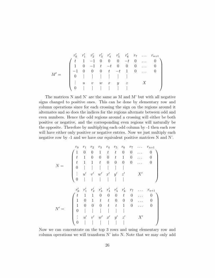
M ′ =

r′0 r′1 r′2 r′3 r′4 r′5 r′6 r7 . . . rn+1

t 1 −1 0 0 0 −t 0 . . . 01 0 −1 t −t 0 0 0 . . . 0−1 0 0 0 t −t 1 0 . . . 00 | | | | | |... u v w x y z X0 | | | | | |

The matrices N and N’ are the same as M and M’ but with all negative

signs changed to positive ones. This can be done by elementary row andcolumn operations since for each crossing the sign on the regions around italternates and so does the indices for the regions alternate between odd andeven numbers. Hence the odd regions around a crossing will either be bothpositive or negative, and the corresponding even regions will naturally bethe opposite. Therefore by multiplying each odd column by -1 then each rowwill have either only positive or negative entries. Now we just multiply eachnegative row by -1 and we have our equivalent positive matrices N and N’.

N =

r0 r1 r2 r3 r4 r5 r6 r7 . . . rn+1

1 0 0 1 t t 0 0 . . . 0t 1 0 0 0 t 1 0 . . . 0t 1 1 t 0 0 0 0 . . . 00 | | | | | |... u′ v′ w′ x′ y′ z′ X ′

0 | | | | | |

N ′ =

r′0 r′1 r′2 r′3 r′4 r′5 r′6 r7 . . . rn+1

t 1 1 0 0 0 t 0 . . . 01 0 1 t t 0 0 0 . . . 01 0 0 0 t t 1 0 . . . 00 | | | | | |... u′ v′ w′ x′ y′ z′ X ′

0 | | | | | |

Now we can concentrate on the top 3 rows and using elementary row andcolumn operations we will transform N’ into N. Note that we may only add

26

column 1 to the other columns, or multiply it by -1 or t, as to not changethe values of the vectors u-z. We begin by swapping row 1 and 3 in N’t 1 1 0 0 0 t

1 0 1 t t 0 01 0 0 0 t t 1

−→1 0 0 0 t t 1

1 0 1 t t 0 0t 1 1 0 0 0 t

Multiply row 1 by -1 and add it to row 2 −→

1 0 0 0 t t 10 0 1 t 0 −t −1t 1 1 0 0 0 t

Multiply row 2 by -1 −→

1 0 0 0 t t 10 0 −1 −t 0 t 1t 1 1 0 0 0 t

Multiply column 1 by -1 and add it to column 7 −→

1 0 0 0 t t 00 0 −1 −t 0 t 1t 1 1 0 0 0 0

Add row 3 to row 2 −→

1 0 0 0 t t 0t 1 0 −t 0 t 1t 1 1 0 0 0 0

Add column 1 to column 4 −→

1 0 0 1 t t 0t 1 0 0 0 t 1t 1 1 t 0 0 0

[6] And thus we have shown that N’ is equivalent to N which we know isequivalent to M. Finally since all the Reidemeister moves yields matricesthat are equivalent to the original Alexander matrix and since we only haveused elementary row and column operations, where we only multiply by ±tkthat is all we have changed the determinant by, which puts the polynomialwithin the definition.

Note that in this proof we do not use the fact that we may remove anytwo neighbouring regions to gain the Alexander matrix, thus we will notrigorously prove that statement here, but refer the reader to the proof Longprovides in Topological invariants of knots: three routes to the AlexanderPolynomial [6]. However it can also now be proved by using the Reidemeistermoves.

27

Now that we know that the Alexander polynomial is a knot invariant aquestion of interest is if it can tell all nontrivial knots apart from the unknot.Unlike the Jones polynomial where it hasn’t been proven if it distinguishes allnontrivial knots from the unknot or not, for the Alexander polynomial thereexist known nontrivial knots with Alexander polynomial 1, as for examplethe (-3,5,7)-pretzel knot, see fig.18 [5]

Figure 18: The (-3,5,7)-pretzel knot [10]

12 Complements of knots as invariants

The last knot invariant we will look at but not prove, is quite different fromthe other ones since now we will be looking at the complement of the knotK in R3. We call it M and it is defined as R3 − K or alternately S3 − Kdepending on which space we are currently working in. These complementswill be 3-manifolds, which are spaces where around any given point in themanifold there exists a neighbourhood homeomorphic to a ball in Euclidean3-space also contained in the manifold. So spaces such as R3 and S3 are also3-manifolds.[5] One neat aspect of working in S3 is that we have a compactspace, and if we take the the open tubular neighbourhood of K, let us call itN, and define M = S3 − N then the resulting 3-manifold will be compact.[3] For the complements of knots there is the following theorem by Gordonand Luecke stating:

Theorem 16. If two knots have homeomorphic complements then they areequivalent. [1]

We will not prove this theorem here but note that it exists. One shouldnote that this theorem would not be able to distinguish between mirror-images of knots unless we demand that there is an orientation-preserving

28

homeomorphism between the complements, and not just a homeomorphism.[1] However we can note that the reverse of the theorem is rather intuitive.We know that if two knots are equivalent then there exits an ambient isotopybetween them, this implies that there is a orientation-preserving hoemor-phism from S3 to S3 taking the knot K1 to K2. This implies that S3 −K1

is orientation-preserving homeomorphic to S3 −K2. In this section we willmove on to look at hyperbolic knots. These are knots whose complementis hyperbolic, meaning that they have both a hyperbolic geometry anda hyperbolic metric. This means among other things that lines are takento mean geodesics and given a line and a point not on the line, then thereare at least two lines that are parallel to the first line that goes through thepoint. Another interesting fact is that all triangles in a hyperbolic geometrywill have an angle-sum of less than 180◦. [8] This also means that distancewill be measured differently compared to our regular Euclidean metric,and depending on which hyperbolic space we look at, it might be measuredin different ways. Even though all of these aspects of hyperbolic geometryare really interesting they are not the reason why we are using these com-plements. It is rather due to the fact that any complete hyperbolic structurewe find on our knot complement M is the only structure there is.[7] This wasstated by Mostow as a theorem and it implies that geometric invariants wefind for the complements will work as knot invariants as well.

Theorem 17. If Mn1 and Mn

2 are complete hyperbolic manifolds with finitetotal volume, any isomorphism of fundamental groups φ : π1(M1) −→ π1(M2)is realized by a unique isometry. [3]

The invariant that arises specifically from this fact is the hyperbolic vol-ume of the hyperbolic knot where knots which aren’t hyperbolic are assignedthe volume 0. Creating the complement is usually done by gluing togethersets of hyperbolic tetrahedra in such a way that faces match and the dis-tance function within each individual tetrahedra match the ones glued ontoit. These tetrahedra are in turn gained form the knot itself through certainmethods which decomposes the knot complement into the set of tetrahedra[7] but we won’t go into further detail here. The hyperbolic volume is thencomputed as the sum of the volumes of the individual tetrahedra and willalways be a positive real number. This invariant is very efficient in tellinghyperbolic knots apart, although it has a few hyperbolic knots between whichit cannot distinguish such as mutant knots. These knots are made by flip-ping a tangle in a hyperbolic knot and does unfortunately have the same

29

hyperbolic volume, even though they might not be equivalent. [5]

13 Summary

As a conclusion to this essay I’d like to discuss what this study has yieldedwith respect to the thesis and the aim of the essay. Our question was ”Howcan one tell different knots apart?”. This can mainly be done through variousknot invariants, which will guarantee that two equivalent knots will be in thesame equivalence class of the invariant. These invariants could be applied tothe two dimensional projection of the knot, the complement of the knot orthe knot itself. However it soon became clear that these invariants weren’tperfect. Some, like the Crossing number demands that we find the projectionswith the least crossings. But as we know the Reidemeister moves we use toget from one projection to another can go on for a long time and we stillwon’t be sure if there is one with a lower crossing number or not. It is onlywhen we know all of the knots with known lower crossing numbers and canbe sure that our knot does not belong to that set that we can determine itscrossing number. Thus invariants need to be easy to compute, but they alsoneed to be able to tell many different knots apart. For example the invariantwhere all knots received the same constant is easy to compute but it wont tellany knots apart since they all belong to the same equivalence class. So whenlooking at the invariants it became relevant to discuss those two aspects aswell as actually proving that they indeed were invariants. It was shown thatReidemeister moves are a good way to prove that the invariants indeed areknot invariants. This is because the Reidemeister moves doesn’t create newknots, but rather act as an planar isotopy between the projections of theknot. Thus if an invariant was the same before and after the application of aReidemeister move, it would fulfill the criteria for a knot invariant. We wereable to apply this method of using the Reidemeister moves to all invariantsthat we presented in this paper but one. This invariant was applied tothe complement of the knot and was thus completely independent of possibleprojections of the knot. In the cases where it was applied it was used more orless directly. In the case of tricoloring it was used very directly since we coulddisplay all the possible cases and show that the invariant remained unchangedunder each Reidemeister move. With the Bridge number and crossing numberhowever we had to take a slightly different approach since both RI and RIIdirectly changes both the number of crossings and bridges. Thus we had to

30

conclude that if a bridge- or crossing number had been correctly assignedthen the Reidemeister moves would only be able to increase these numbers.This is however not a problem since both of these invariants are based on theprojection which produces the lowest number. With the polynomials, againa direct approach was possible. That is because the Reidemeister moves onlychanges the knot locally, and we were able to ”isolate” the affected part ofthe knot and then compare the computations before and after the move forthat part.

The last invariant was a bit more difficult to grasp and explain since itapplies a lot of mathematics that were new to me and therefore demandedmore time. Hence the section is a bit thin, and if given the opportunitysometime in the future, I would like to look into it more. However part ofthe aim was to deepen my knowledge of topology and geometry and that hasindeed been fulfilled. A part that I in particular would like to look into moreis how the orientation-preserving homeomorphism between the fundamentalgroups of knot complements looks and works. As well as the fundamentalgroups themselves. I believe that if that part was made clearer then theconnection would be easier to make.

All in all we can conclude that one can tell different knots apart in manydifferent ways, however as of yet no method can single-handedly tell all dif-ferent knots apart, or even all nontrivial knots apart from the unknot, thoughthe Jones polynomial might be able to do this, we await a proof which cansay for sure if that is the case. Thus this part of knot theory is still relevant,partly due to its connections to other fields such as chemistry, biology andquantum computation, but also because it is fun to work with!

31

References

[1] C. McA. Gordon and J. Luecke. Knots are determined by their comple-ments. Journal of the American mathematical society, 1989.

[2] 3-coloring and other elementary invariants of knots. 1998. url: http://matwbn.icm.edu.pl/ksiazki/bcp/bcp42/bcp42120.pdf. (ac-cessed: 31-05-2019).

[3] William P. Thurston. The Geometry and Topology of Three-Manifolds.2002. url: http://www.msri.org/publications/books/gt3m/.(accessed: 13-06-2019).

[4] Heiner Zieschang Gerhard Burde. Knots. Walter de Gruyter, 2003.isbn: 3 11 017005 1.

[5] Collin C. Adams. The knot book, an elementary introduction to themathematical theory of knots. American Mathematical Society, 2004.isbn: 0-8218-3678-1.

[6] Edward Long. Topological invariants of knots: three routes to the Alexan-der Polynomial. Manchester University, 2005.

[7] Jessica S. Purcell. Hyperbolic Knot Theory. Brigham Young University,2010.

[8] David C. Kay. College Geometry, A unified development. CRC Press,Taylor & Francis Group, 2011. isbn: 978-1-4398-1911-1.

[9] Daniel Amankwah. The Jones polynomial and its limitations. AfricanInstitute for mathematical Sciences, 2014.

[10] Carl H. Brans Torsten Asselmeyer-Maluga. “How to include fermionsinto General relativity by exotic smoothness”. In: (Gen.Rel.Grav. 47(2015) no.3, 30 2015).

[11] E. L. Xiaoyu Qiao. Knot Theory Week 2: Tricolorability. 2015. url:http : / / web . math . ucsb . edu / ~padraic / ucsb _ 2014 _ 15 / ccs _

problem_solving_w2015/Tricolorability.pdf. (accessed: 01-06-2019).

[12] J. C. Cha and C. Livingston. Table of Knot Invariants. url: http://www.indiana.edu/~knotinfo/. (accessed 14-06-2019).

32

[13] Abhijit Champanerkar. The geometry of knot complements. url: https://www.math.csi.cuny.edu/~abhijit/talks/knot- geometry-

h.pdf. (accessed 13-06-2019).

[14] Eric W. Weisstein. Reducible Crossing. url: http : / / mathworld .

wolfram.com/ReducibleCrossing.html. (accessed 02-06-2019).

[15] Wikipedia. Ambient Isotopy. url: https://en.wikipedia.org/wiki/Ambient_isotopy. (accessed: 17-05-2019, last edited: 12-09-2017).

[16] Wikipedia. Knot (mathematics). url: https://en.wikipedia.org/wiki/Knot_(mathematics)#Formal_definition. (accessed: 07-05-2019, last edited: 18-02-2019).

33