Lattice-gas crystallization

Journal of Statistical Physics, Vol. 81, Nos. 1/2, 1995

Lattice-Gas Crystallization

J. Yepez ~

Received August 30, 1994;final April 27, 1995

This paper presents a new lattice-gas method for molecular dynamics modeling. A mean-field treatment is given and is applied to a linear stability analysis. Exact numerical simulations of the solid-phase crystallization are presented, as is a finite-temperature multiphase liquid-gas system. The lattice-gas method, a discrete dynamical method, is therefore capable of representing a variety of collective phenomena in multiple regimes from the hydrodynamic scale down to a molecular dynamics scale.

KEY WORDS: Lattice-gas automata; discrete hydrodynamics; multiphase fluids; complex fluids; liquid-gas transition; molecular dynamics; crystallization.

1. I N T R O D U C T I O N

This paper presents a theory of lattice-gas dynamics that includes interparticle potentials. The microscopic lattice-gas dynamics is a highly discrete form of traditional molecular dynamics. All the usual dynamical quantities appearing in the traditional theory are discrete in the case of a lattice gas. It is well known that in lattice gases these discrete quantities include space, time, and momentum. Here the notion of a discrete field is introduced and an analytical theory is presented to describe emergent macroscopic dynamics. The field concept is shown to be quite useful. In particular, the field concept is useful in describing our novel lattice gas with multiple long- range interactions with different ranges and polarity. This new lattice gas possesses a liquid-solid transition and can be used as a new general method of simulating molecular dynamics. The theoretical possibilities for such a lattice gas open the subject of exactly computable modeling to the areas of dynamical solid-state systems.

Phillips Laboratory, Hanscom Field, Massachusetts 01731. E-mail: [email protected].

255

0022-4715/95/1000-0255507.50/0 �9 I995 Plenum Publishing Corporation

256 Yepez

It is known that interparticle potentials can be modeled by including a single anisotropic fixed-range interaction in the lattice-gas dynamics for discrete momentum exchange between particles. The simplest theoretical model of this kind is the Kadanoff-Swift-Ising model. (8~ An attractive fixed-range interaction was used in a lattice-gas automaton by Appert and Zaleski (-'~ in 1990 to model a nonthermal liquid-gas phase transition. The use of attractive and repulsive fixed-range interactions of this sort extended the lattice-gas dynamics to a finite-temperature liquid-gas transition where a complete pressure, density, and temperature equation of state is modeled, and the complete liquid-gas coexistence curve is analytically predicted through a Maxwell construction. (ls~ Our finite-temperature liquid-gas lattice gas is presented here for pedagogical reasons as well as to validate the theoretical method presented. Lattice-gas crystallization is introduced as a direct generalization of the finite-temperature liquid-gas lattice-gas model.

This paper is organized in basically two parts. The first part of the paper up to and including Section 4 is familiar to the lattice-gas community and is given here as review material for the subject of lattice gases with purely local collisions. The rest of the paper presents new results, using a new theorem referred to here as the lattice multiple theorem, presented in Appendix A. This theorem is useful for determining the linear response of a lattice gas with long-range interactions. Appendix B describes in some detail an explicit numerical method for implementing the simplest of long- range interactions: the bounce-back and clockwise orbits.

2. LATTICE-GAS A U T O M A T O N : AN EXACTLY C O M P U T A B L E D Y N A M I C A L SYSTEM

A Boolean formulation of an exactly computable dynamical system, known as a lattice gas, may be stated in a way that is consistent with the Boltzmann equation for kinetic transport. In essence the lattice-gas dynamics is a simplified form of molecular transport, as we restrict ourselves to a discrete cellular phase pace. The macroscopic equations, in particular the continuity equation and the Navier-Stokes equation, are obtained by ensemble averaging over a discrete microdynamical transport equation for number Boolean variables. The scheme employs the finite- point group symmetry of a crystallographic spatial lattice. It is somewhat inevitable that to obtain an exactly computable representation of fluid dynamics one must perform a statistical treatment over discrete number variables.

Before introducing the basic lattice-gas microdynamical transport equation, let us give some notational conventions. We consider a spatial

Lattice-Gas Crystallization 257

lattice with N total sites. The fundamental unit of length is the size of a lattice cell l and the fundamental unit of time z is the time it takes for a speed- one particle to go from one lattice site to a nearest neighboring site. Par- ticles with unit mass m propaga te on the lattice. The unit lattice propaga- tion speed is denoted by c = l/z. Particles occupy this discrete space and can have only a finite number B of possible momenta . The lattice vectors are denoted by e~,-, where a = 1, 2 ..... B. For example, for a single-speed gas on a tr iangular lattice, a = 1, 2 ..... 6. A particle's state is completely specified at some time t by specifying its position on the lattice xi and its m o m e n t u m Pi = rnceai at that position. The particles obey Pauli exclusion, since only one particle can occupy a single m o m e n t u m state at a time. The total number of configurations per site is 2 B. The total number of possible single- particle m o m e n t u m states available in the system is N t o t a I = BN. With P particles in the system, we denote the filling fraction by d = P/Ntotal.

The number variable, denoted by n~(x, t), takes the value of one if a particle exists at site x at t ime t in m o m e n t u m state rnc~a, and takes the value of zero otherwise. The evolution of the lattice gas can then be written in terms of n, as a two-par t process: a collision and a streaming part. The collision par t reorders the particles locally at each site,

n'~(x, t ) = n~(x, t ) + ~ ( n ( x , t)) (1)

where ~ a represents the collision opera tor and in general depends on all the particles n at the site. So as a shor t -hand we suppress the index on the occupat ion variable when it is an argument of ~?a(n(x, t)) to represent this general dependence. In the streaming par t of the evolution the particle at position x "hops" to its neighboring site at x + l~a and then time is incremented by 3,

n'(x + l ~ , t + z) = n.(x, t) + s t)) (2)

Equat ion (2) is the lattice-gas microdynamical t ranspor t equat ion of motion. The collision opera tor can only permute the particles locally on the site, since we wish the local particle number to be conserved before and after the collision.

We construct an nth-rank tensor composed of a product of lattice vectors (13)

E ~ = Eg, ...i, = ~ (e , ) i~ . . . (e,) i , (3) a

where a = 1 ..... B. All odd-rank E vanish. We wish to express E ~2") in terms of Kronecker deltas, J0 = 1 for i = j and zero otherwise. We can turn this

258 Yepez

problem of expressing the E-tensors in terms of products of Kronecker deltas into a problem of combinatoric counting. We use the tensors

z/,~. = ~ u (4)

A~kl = ~O~k~ + ~kC~;I +GtG; (5)

and so forth. Then we know that if E is isotropic, it must be proportional to d

E ~2"1 oc d ~2,'J (6)

and that the constant of proportionality may be obtained by counting the number of ways we could write a term comprising a product of n Kronecker deltas. Consider, for example, the case 17=2. Since the Kronecker delta is symmetric in its indices, the following four products are identical: ~0.~kl= ~i;j~/, = ~j~C~kl= C~jfll,. The degeneracy is 2 2. Furthermore, the order of the Kronecker deltas also does not matter since they commute; that is, ~USk~=8k~SV. The degeneracy is 2!. For the case where n is arbitrary, there are 2" identical ways of writing the product of n Kronecker deltas. For each choice of indices, there are an additional n! number of ways of ordering the products. Therefore, the total number of degeneracies equals 2"n! = (2n)!!. The total number of permutations for 2n indices equals (2n)!. So from this counting procedure we know that zl t2"~ consists of a sum of (2n!)/(2n)!! = (2n -- I )!! terms.

In general, the lattice tensors are

E 2 . + 1 ~ 0

E 2 . _ _

D ( D + 2 )

B

. ( D + 2 n - - 2

(7)

,~-'" (8)

3. MESOSCOPIC D Y N A M I C S

To analyze theoretically the lattice-gas dynamics, it is convenient to work in the Boltzmann limit where a field point is obtained by an ensemble average over the number variables. That is, we may define a single-particle distribution function, f~ = (n, , ) , resulting from an ensemble of initial conditions and the neglect of correlations, with the averages taken over the ensemble.

It is essential to determine the macroscopic limit of the microdynamical transport equation (2) and to see how it leads to noncompressible viscous Navier-Stokes hydrodynamics; for a lengthier treatment of this see Frisch et aL (6~


Using the Boltzmann molecular chaos assumption, we find that the averaged collision operator simplifies to ( ~ a ( n ) ) = f 2 a ( ( n ) ) , and by coarse graining and Taylor expanding (2) we obtain the lattice Boltzmann equation

c3tf,, + ce . iOi f . , = Q,,(f) (9)

We write the particle number density, momentum density, and moment flux density in terms of the single-particle distribution function as follows:

m ~ , f . = p (lO) a

mc ~ eoif~ = pvi (I I ) a

m c 2 ~ , e,,ie,~jf,, = H O. (12) a

Now following Landau and Lifshitz, t91 we know that in standard form we must be able to write the momentum flux density tensor as follows:

mc2 ~ e,,ie,,Jf,, = Pfio" + privy-- a~ (13) a

where in (13) the first two terms represent the ideal part of the momentum flux density tensor and a ~ = r l ( O ~ v j - a j v ~ ) is the viscous stress tensor. Alternatively the momentum flux density tensor may be written

Hi) = m c 2 ~, eoie,,y f , , = --tr ~ i + pv~v.i (14) a

where trv is the pressure stress tensor

a U = -p6;y + q(O; vy + 0~ vy) ( 15 )

The general form of the single-particle distribution function, appropriate for single-speed lattice gases, is a Fermi-Dirac distribution. Fundamentally, this arises because the individual digital bits used to represent particles satisfy a Pauli "exclusion principle. Therefore, the distribution must be written as a function of the sum of scalar collision invariants ~ + f l e a ~ v i , implying the form

1 f a - 1 + e ~+pe'v' (16)

260 Yepez

Taylor expanding (16) about v = 0 to fourth order in the velocity and equating the zeroth, first, and second moments offa to (10), (11), and (12) respectively, we determine the parameters 0~ and ft. The inviscid part of the lattice-gas distribution function becomes

(~r 'eq'~ ideal - - n + nD Ja , ' L G A - - - '~eaiVi "~- g nD(D + 2) d,,i~ujvivj 2c2B

n ( D + 2 ) , g 2c2------ff-v- (17)

where

D 1 - 2 d g ~ D + 2 1 - d (18)

That is, using p = mn for the density and cs = c/v/D for the sound speed, we find the moments of the lattice-gas distribution

m ~,/feq~ideal (19) ~da / L G A ~ P a

mc ~ e~,i,., r LOA = PVi (20) a

( f e q ~ i d e a l __ 2 V - mc2/ ,ea iea jxaa Z L G A - - P C s 1 - - g (~O."}-gpvivj a

(21)

The lattice-gas automaton almost produces the correct form for the momentum flux density tensor, except that H,j appears to have a spurious dependence on the square of the velocity field, (1 -g(v2/c2)) with a factor g arising as an artifact of the discreteness of the number variables. Working directly in the Boltzmann limit and using only symmetry arguments, it is possible to fix this problem.

The macroscopic equations of motion are then determined from mass conservation (continuity equation) and momentum conservation (Euler's equation)

O,p + ai(pv,) = 0 (22)

and

a,(pv;) + 0/Hu= 0 (23)


Substituting (21) into Euler's equation (23) gives us the Navier-Stokes equation for a viscous fluid

p(O,v i + gvjOjv,) = -Oip + qO~-vi (24)

given a nondivergent flow (OiD i = 0 ) appropriate to the incompressible fluid limit and where the pressure is

p=pc~, l + g ~ (25)

A general expression for the shear viscosity r /for a single-speed lattice gas has been derived by H6non. (7)

In any lattice-gas simulation, one typically obtains a realization of the macroscopic dynamical variables by block averaging in both space and time over the mesoscopic variables. In this way, for example, a momentum map can be produced so that the dynamic evolution of the fluid can be monitored. The size of the coarse-grain block affects the resolution with which one can observe the system, but of course does not at all affect the underlying dynamics. If too small a coarse-grain block size is used, more fluctuations in the macroscopic variables occur.

4. LATTICE BGK EQUATION

We wish to consider a dynamical transport equation for the particle distribution function given in the previous section. We have a lattice Boltzmann gas defined on a discrete spatial lattice. Restricting ourselves to a single-speed lattice-gas system, the lattice BGK equation is

~ t "~- s aiO i f a = - - ~ ( f o - f aeq ) (26)

This equation was introduced in 1954 by Bhatnager, Gross, and KrookJ 3"~~ A way to obtain (26) was introduced by Chen etal. ~5) by expanding the lattice Boltzmann collision term to first order about the equilibrium distribution and assuming it diagonal.

It is possible to fix the anomaly in the fluid pressure that occurs in the lattice-gas automaton. Chen et aL (4~ introduced a pressure-corrected equilibrium distribution having the following Chapman-Enskog expansion

(r162 _ B +riD nD(D + 2) daiO.jvivi_ nD vZ d a ) B G K - - -~eaioi"~- 2c2B (27)

262 Yepez

which satisfies

m ~ .,,, vc = P 1 - (28)

]T/C E t , ' eqx idea l __ e,itJ,, )PC -P/) i (29) a

mcZ ~ eaie,,j,., c'eq~iaeal -- pc~ dO. + pc -- (30) a

Here the definition of the density is modified by the 1 - v2/c 2 factor.

5. DENSITY-DEPENDENT PRESSURE IN THE BOLTZMANN LIMIT

Here we exploit the analytical facility of the lattice Boltzmann approach and show that the addition of a convective-gradient term in the lattice Boltzmann equation allows one to model a hydrodynamic gaseous flow governed by a general equation of stateJ ~4) The pressure may have a nonlinear dependence on the local density. It is possible to generalize this to a multispeed lattice gas or a to single-speed lattice gas coupled to a heat bath so that the pressure dependence includes the local temperature as well.

The equation of state for the isothermal gas is

p=c~.p (31)

We now wish to consider how we may alter the lattice-Boltzmann equation to allow for a more general equation of state. Let us add an additional term, P,(x, x + reo), to the r.b.s, of (9),

O,f.(x, t )+ce.iOif .(x, t) = 1 [g2.(x, t ) + P . ( x , x+re~, t)] (32) T

P. depends on the local configuration of the system at position x as well as on the local configuration at a remote position x + re.. We assume that the values of ~, at x and x + re. are independent and that therefore Pa can be factorized 2

Pa(x, x + re., t )= ~(x) ~(x + re.) (33)

2 The effect of long-range interactions on f . (x) will actually depend on local configurations at x + re. and at x - re.. So we could write the full form of the long-range part of the collision operator as �89 [ ~b(x) ~(x + re . ) - ~ ( x - re.) ~b(x)], where the factor of �89 must be included to avoid double counting when doing any directional sums ~ , since qJ here does not have any directional dependence. According to Theorem 1 in Appendix A, upon expanding ~O(x) qJ(x+_reo), both terms would add to remove the �89 factor, so using P o = ~b(x) ~(x+re.) in the present calculation ultimately gives the same result. In Appendix B, where we give the microscopic long-range part of the lattice-gas collision operator, the microscopic ~b does have directional dependence, so we use the full form there.


In a single-speed lattice-gas model such as we have been considering, P . is a function of the local density. In a single-speed model coupled to a heat bath, P~ may depend on the local temperature as well/~5)

We wish to constrain the form of P . so as not to violate continuity. We require

P,, = 0 (34)

and when Oif. = 0,

e.iP. = 0 (35) a

Constraint (35) is required only under uniform filling conditions; i.e., for general situations Z. e,.P,, is nonzero. In the uniform flow limit the lattice- Boltzmann equation reduces to

O,f.(x, t) =-1 [12.(x, t) + P(x, x + re., t)] (36)

where we have taken the directional dependence of the long-range colli- sional term to occur only in its argument, P . ( x + r e . ) ~ P(x+re.) . We assume the probability of a long-range collision depends only the density at the spatial location of a momentum transfer event and not on the direction of the momentum transfer. That is, we require the interaction distance to be of sufficiently long range that the approximation of local isotropy in the particle distribution is valid. Summing over all lattice directions and using constraint (34), we have maintained the collision property that

~' I2~ta' = y" ((2. + P.) = 0 (37) a

Thus, for arbitrary flows, summing the lattice-Boltzmann equation (32) over all directions preserves continuity

0, y ' f~ + c Z e . ,0;f . = 0 (38)

O,p + O~(pvi) = 0 (39)

where we have used (37). Multiplying the lattice-Boltzmann equation by ea~ and then summing

over directions gives

O, Z e. ,L( x, t) + cOj Y" e.,eajL(x, t)

1 = - r t) ~ e.it~(x + re., t) (40)

72 a

264 Yepez

Using Theorem 1 in Appendix A we can expand the r.h.s.,

O, Z ea,L(x, t) + cOj Z e,ge~jL(x, t) a a

= + ; ~(x, t) - ~ / ' -

Therefore, we again arrive at Euler's equation

0,(pui) + Oj(II u) = 0 (42)

but with an augmented momentum flux density tensor

,l :_mc2 2 eo, eo, L-mc2 ?-)?-U- o \ z / \ 2 /

x rS• f dxk ~9(x, t) Ok(rO) -D]2 iD/2(rO) ~b(x, t) (43)

Since the additional term in the momentum flux density tensor is diagonal, it can only impart an effective density-dependent pressure.

Defining a configurational potential energy as

V(x) = mc2B \ l . / \ 2 7

x f dxk Ip(x, t) Ok(rO)-9/2 Io/2(rO) ~(x, t) (44)

we obtain from Euler's equation (42) the viscous Navier-Stokes equation for nonideal fluids

Ot(PVi) 4- Oj(pvioy) : -Oi(c~p 4- V(p)) 4- pvO2vi (45)

Therefore, we have arrived at a general equation of state defined by the potential energy function V(p) where there is an interparticle force F;(x) = -0~ V(p(x)). The form of the density-dependent pressure directly follows,

p(p) 2 =cup + V(p) (46)


With this methodology, we can model a system with a general equation of state with completely local dynamics described by the generalization of (26),

-g

f~(x + 1~, t+ z)=f~(x, t ) - ~(f ,(x, t)--f;q(x, t))

+ ~k(x, t) q,(x + rea, t) (47)

In the Boltzmann limit, the analysis itself does not indicate the form of V in (46) (or more to the point, does not indicate the form of ~b), but does show it is possible to have a lattice gas that has Navier-Stokes dynamics as its macroscopic limit with a density-dependent pressure (45). This is the motivation needed to develop a more complete microscopic description. With a lattice-gas automaton microscopic description, the interparticle force -0~ V(p) may be caused by long-range momentum exchange between two particles. Calculating the probability of such momentum exchange events should provide a way to determine ~.

Note that in the mesoscopic regime in which the Boltzmann equation is applicable, the lowest order expression for V is proportional to Oz. That is,

=----~--mc2B(;) V(x) ~ dXk O(x) Ok~k(x) (48)

o r

V(x) = --~-- r (49)

A similar calculation was done by Shan and Chen, (~21 who verified their analysis by comparing with data taken from lattice BGK simulations. They also presented exact calculations for the liquid-gas interface profile and surface tension. In the following section we take another viewpoint and write an alternate expression for the potential energy, but one that is also proportional to ~,2. This alternate view of the potential energy will help toward developing the lattice-gas automaton microscopic description.

6. INTERACTION ENERGY

We introduce a potential energy due to nonlocal two-body interactions

H'=~ ~. ~ (1-f~(x))fo(x) V,b,,,,(1-f,,(x'))f,,(x') (50) ( x x ' ) (, abmn >

266 Yepez

where V.b.,,,= VAabmn and A.b .... is either _1 or vanishes for any set {abmn} that violates mass, momentum, or energy conservation. H ' accounts for the potential energy between particles incoming along lattice directions b and n and outgoing along a and m and is therefore restricted to two-body interactions.

We now try to justify the form of H ' and in so doing develop a microscopic description of the lattice gas with long-range interactions. We require

pi= -Oi H' (51)

H ' is thought of as the configurational potential energy due to momentum transfers between two locations. The momentum exchange per unit time between two points x and x ' in the fluid is

6p i= mo~ -- mt)iin (52)

in where the incoming and outgoing velocity states are quantized: v~ =ceb~ O1.1l and v~ = eeoc. The probability if(x) of there being a local momentum

change at some point x depends independently on the probability fo(x) that there is a particle in velocity state ceb~ and the probability 1 - f ~ ( x ) there is not a particle in velocity state ce.i. So in this factorized approximation that neglects particle-particle correlations, we write

~k(x) = (1 - f ~ ( x ) ) fb(x) (53)

.! As a long-range momentum exchange event involves two sites x and x , we can define the vector r~=reo~=x~-x~, and therefore the parallel and perpendicular components of the local momentum exchange are

~ p t l = 6 p - ~ (54)

fie• = 10p• fl (55)

The two components of the force mediated by the long-range momentum exchange could be interpreted as created by two separate fields

6E=6Ptl(r) c f (56) l

OB - fip• c ~ • ~ (57) 1

where 6pl I and 6p• are written as a function of r since any kind of func- tional dependence is allowed provided enough detail is specified for the


automaton interaction rules. We have explicitly written the forms of the parallel and perpendicular components of a lattice-gas force field to stress an analogy with the classical theory of electromagnetism, where the electric and magnetic fields are expressed, for a differential element of charge and current element, respectively, by the laws of Coulomb and Biot-Savart

dE = .6_~_Q_2 ~ (58) 4rtr

dB = 4--~r2 fil x f (59)

Using (53), we can write the total momentum change as a field itself

@ i ( x , x ' ) = - m c ~ (e , , i -ebi+e. , i -e , , i ) (1- f . (x ) ) ( abmn )

xfb(x) Aab.,,,(1 -- f,,,(x') ) f,,(x') (60)

Note that the momentum change is zero for a fluid with uniform density due to the symmetry of the lattice. For central-body interparticle momentum exchanges, in the Boltzmann limit we can then approximate the configurational potential energy as

ri t~pi g ( x , x ' ) - -

/7

,

( abmn )

x ( 1 - f~) fbA.o.,,,(1 --f..) f,, (61)

where r is the range of the interaction. For a system locally isotropic in its particle distributions, letting ~b(x)= ( 1 - f ( x ) ) f (x) , this may be simplified to

V(x.x')=-~mc- y~ ~ ~. (~,o-~ + ~.,- ~,,) < abmn > < abmn )

x A.b.,,,tp(x ) O(x') (62)

which is suitable for a bulk description of the fluid. Now the form of H' follows if we sum over all pairs ( x x ' ) and define

V'ob,,,,,=mcZ (~) f ' ( ~ - - ~ b + ~,,,--~,,) A.b ..... (63)

so that

H'= ~ V(x ,x ' )= ~" Y'. O(x)V.b.,,,~b(x') (64) ( x x ' ) (xx'> (abmn)

268 Yepez

7. E-FIELD C O N S T R U C T I O N

It is possible to define a field that exists in a lattice gas that has long- range m o m e n t u m exchanges occurring. The notion is to consider each lattice-gas particle as having a delta-function-type field that exists only at certain fixed ranges and certain fixed angles. Therefore, the lattice-gas particle has a highly anisotropic field. However, in the coarse-grained limit obtained by averaging over many particles, a valid description of a con- tinuous field emerges. Of course, if there are no gradients in the coarse- grained density of the system, the field must necessarily vanish.

The field at posit ion x due to a particle at position x' along the lattice direction a is a delta function

e.,(x; x ) = - - f - ~ e(~r) 6(x - x ' - r~O,,) e,,, (65)

Tha t is, the discrete field must be directed along ~, and must be a distance r~ from the source, or x = x' + r~O,,. The total field is obtained by considering all the possibilities where a particle could contribute. The sum over a is necessary to account for multiple interaction ranges, where 0c(a) denotes the strength of the interactions at range r~. Thus to obtain the total field we must sum over all directions and integrate over all positions

Ei(x) = ~ f dx' ~(x') e.i(x; x') (66) u

o r

m c 2

E,(x) = - - f - y" e (a) ~ e. iO(x -- r~0a) (67)

Using Theorem 1 in Appendix A, we can evaluate the directional sum and express the field as a gradient of a scalar quanti ty

El(X) =-Oilmc2B~ix.(;)*/2(r.O)-n/2Io/2(r~O)O(x)] L g

(68)

where p,, is defined as


N o t e that /~ > 0 for attractive interactions and p < 0 for repulsive interactions. Since E; = Oil, the field's scalar potential is

['~'k<a ~b=-mc2B2lG~-~j (r=O)-DI2lol2(r=O)~s(x) (70)

a

= - m c 2 B ~ l ~ a 0 4 2D(D+ + ... (71)

The field E; and the event probability ff = d(1 - d ) appear in the Navier- Stokes equations as follows:

,[( O,(pvi)+Oj(gpv~vs)=-c~O ~ p l + g ~ +OE~+pvO2v~ (72)

and according to (43), the term OEi when due to central-body interactions can modify only the pressure.

8. STABIL ITY A N A L Y S I S

In this section we consider the linear response of a lattice gas with long-range central-body interactions. The macroscopic equations of motion are (39), (72), and (68), respectively:

O t p + O i ( p v i ) = 0

[( O,(pv~)+Oj(gpv~vj)=--c~Oi I) l+gc . _ +OEi+PVO2v~

E i ( x ) = O, mc 2 - p , , ( r ,~ O ) - D / 2

L ~r

x ID/2(r,,O) ~(•

We treat the effect of the field E,. as a perturbation on a resting equilibrium state where p is uniform and constant and v = 0. Then an e-expansion of the dynamical variables is

vi = eui (73)

P = Po + e0 (74)

~b = ~Oo+e~o (75)

Using ~b = ( 1 - d) d, we have

1 - 2 d o q~ m ~ 0 (76)

822/81/'1-2-18

270 Yepez

where do = po/rnB. Consequently, the linear response equations are

OtQ -J- PoOiUi = 0 (77)

PoOtUi= -c~OiO-I~oOi mc2B t~. (r~a)-~

q~] + poVoOZUi (78) Io12(r~O) x

Then applying 0, to the continuity equation and a; to the Navier-Stokes equation allows us to eliminate ui and to obtain the following second-order equation in Q:

2 _ 2 2 /~. (r .O)-o/2 O, Q - c=O Q + ~bo( 1 - 2do) czO 2

x Io/2(r~O) QI + v~ (79)

In an inviscid fluid (v = 0) with no interparticle potentials (E~ = 0), Q would satisfy the wave equation

Q =po e-i'o'+iki''i (80)

Given a nonzero perturbation, 0 can be Fourier expanded

f do9 dki fie -~'~ (81) Q

and we can replace Q with ~ by taking 0,--+ -ico and 0;--, ik,. Then (79) becomes

= " ' - -- - - I ' : ~ ~ ) ( r . k ) -Di2

x JDi2(r~k) 5] + iCovok2~ (82)

where we have made use of the identity that relates the hyperbolic Bessel function with imaginary argument to the ordinary Bessel function

(iz)-~ I.(iz) = z-"J.(z) (83)

Dividing out ff gives a quadratic equation for co,

v ~ 1 7 6 1 + ~o(1 _2do) D Z/xo_ ( r :k ) -O i~-Jo l=( r .k ) +i c= \C=l

(84)


The dispersion relation for co(k) is then

co= +k 1 + +~o(1 --2do) D ~ p . (r,k)-~ Cs -- "~C2s o

i vOk2 (85) 2cs

The field to lowest order in the interaction range is

mc-B r E,(x) = O~b(x)

This implies that the local force is

~bEi=-O~[2mc:B(~)~b2 ]

(90)

(91)

(92)

In the long-wavelength limit, (85) reduces to linear sound speed dispersion

co = csk (86)

In the absence of long-range interactions, (85) reduces to the dispersion relation for ideal, incompressible, viscous flow

vok'-'~ 1/~- ~ok ~ co=c.,.k I +---;-v- - i - - (87)

4c; J 2

By choosing different ranges and strengths of the momentum exchanges we can adjust the dispersion relation (85) and produce a variety of interesting dynamical behaviors. Therefore, in the macroscopic limit, what principally defines the linear response of a lattice-gas model with long-range interactions is the set of constants co(a) and r~.

9. F INITE-TEMPERATURE L IQUID-GAS MODEL

A simple two-dimensional example is a lattice gas on a triangular lattice. The macroscopic equations of motion for the lattice-gas automaton are

O,p + Oi(pvi) = 0 (88)

O,(pvi) + Oj( gpv~vj) = --O ~ p + pvOZvi (89)

272 Yepez

Since ~ = d( 1 - d), the pressure is a simple polynomial

~ [ ( v2) ~(h)r '2" ] p(d,h)=mc;B d l + g ~ + - - - ~ a t l - d ) 2 (93)

where we have written the pressure depending on the density and a temperature control parameter h that modifies the strength of the interactions, 0~ = 0~(h). This will be discussed in more detail below. It is possible to determine the coexistence curve for such a finite-temperature liquid-gas system. We begin by defining the free energy G as

c a dn Op(n, h) G(d'h)=Jao n On

Using (93) for a fluid at rest, we can carry out the integral to obtain

G( d, h)=mc2B E ~ h ) r ( 4d 3 . 4d3"~ \ - 2d + 3d 2 - ~ - - + 2d 0 - 3do 2 -r --~-)

(94)

A Maxwell construction can be performed by making a parametric plot of the free energy versus the pressure and locating the point at which the curve is double valued. That is, there are two densities, corresponding a rarefied phase and a dense phase, that have the same pressure and minimal free energy. The critical temperature hc can be found by finding the isothermal pressure curve that has an inflection point

o r

Op(d, he) Od 0 (96)

l a(hc) = (97)

2rd( 1 - d)( 1 - 2d)

To verify our theory, we can perform exact numerical simulations of a finite-temperature multiphase system. We can extend an Appert-type nonthermal model to work in a finite-temperature domain by coupling the long-range interactions to a heat bath of variable density, denoted by a parameter h, and by allowing repulsive long-range interactions in addition to the attractive ones. This is done in such a way that the likelihood of an attractive and repulsive interaction goes as (1 - h ) 2 and h 2, respectively.I]5)

+,og(jo) ] ,95,

L a t t i c e - G a s C r y s t a l l i z a t i o n

( a ) o , > 0

2 7 3

( b ) ~ ...................... . ~ -

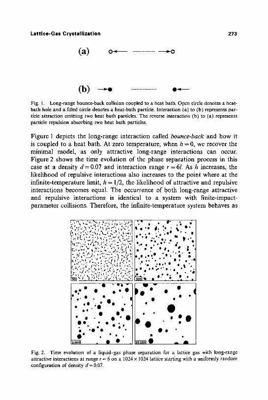
Fig. 1. L o n g - r a n g e bounce-back collision coupled to a heat bath. Open circle denotes a heat- bath hole and a filled circle denotes a heat-bath particle. Interaction (a) to (b) represents p a r -

ticle attraction emitting two heat bath particles. The reverse interaction (b) to (a) represents particle repulsion absorbing two heat bath particles.

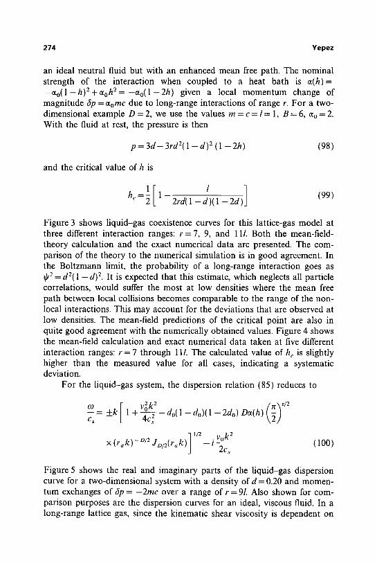
Figure 1 depicts the long-range interaction called bounce-back and how it is coupled to a heat bath. At zero temperature, when h = 0, we recover the minimal model, as only attractive long-range interactions can occur. Figure 2 shows the time evolution of the phase separation process in this case at a density d = 0.07 and interaction range r = 6/. As h increases, the likelihood of repulsive interactions also increases to the point where at the infinite-temperature limit, h = 1/2, the likelihood of attractive and repulsive interactions becomes equal. The occurrence of both long-range attractive and repulsive interactions is identical to a system with finite-impact- parameter collisions. Therefore, the infinite-temperature system behaves as

"~ "L'-- ~''~'~ ' ' ' ; ' ' ' ' . " : 1 . ' , .... ~ -'~4 * g'.'" * * . .~ . IP.', :_" �9 " ' ~ ,,. , ! . . . - . . . , . .

�9 I ~ 1 7 6 �9 o o

~ , ' - . , " " " ~ . ~ - ~ ; ~ . ' t " * " : " " ~ o o ., O . . t. , .,~ r B". ".1 ' ' " ~ o, , , - . j

�9 _ - : ~ * o 8 ' , . . - / ~ . ~ ~ . ; - i �9 . �9 go �9 �9 ~.'~.'~'-..'-~,. :~ ,':'--,::1 ~o-~,, . *" . ,_ ..�9 ."

�9 ~ � 9 e * �9 . �9 �9 O 1 e" O . �9 " ql e 0 �9

oO . l ~ ~ 0 �9 e o " �9

�9 . . �9 o o. �9 " . �9 ~ o,. ; , , , . O O �9 " O �9

O O �9 �9 �9 , ~o0 �9 �9 ~ ~

F i g . 2. T i m e evo lu t ion o f a l i q u i d - g a s p h a s e separa t ion for a lat t ice gas w i t h l o n g - r a n g e

attractive interactions at range r = 6 o n a 1024 • 1024 lattice starting with a uniformly random configuration of density d = 0.07.

274 Yepez

an ideal neutral fluid but with an enhanced mean free path. The nominal strength of the interaction when coupled to a heat bath is cr - % ( 1 - h ) 2 + % h 2 = - % ( 1 - 2 h ) given a local momentum change of magnitude tip = % m c due to long-range interactions of range r. For a two- dimensional example D = 2, we use the values m = c = l = 1, B = 6, 0% = 2. With the fluid at rest, the pressure is then

p = 3 d - 3rd2(1 - d ) 2 ( 1 - 2h) (98)

and the critical value of h is

1E ' 1 h,.= 1 2rd(1 - d ) ( 1 - 2 d ) (99)

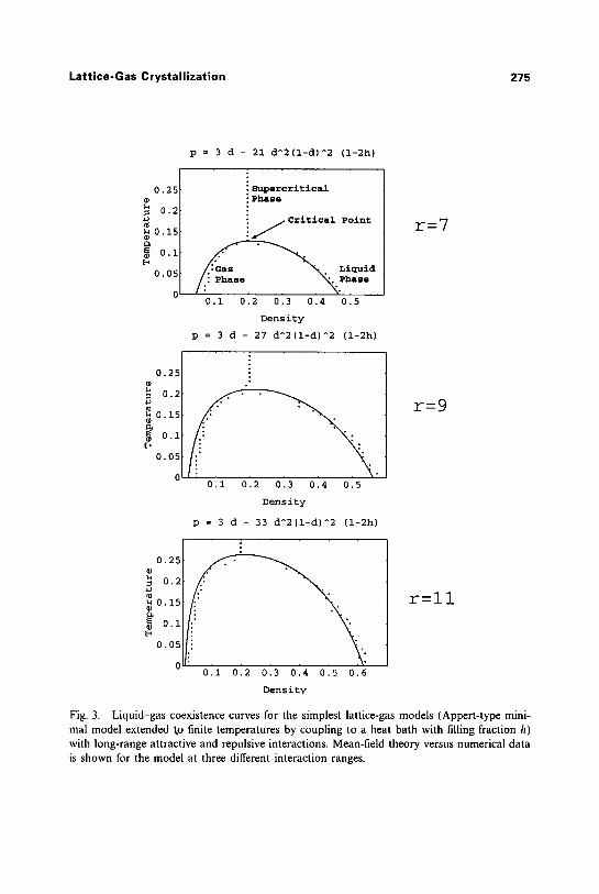
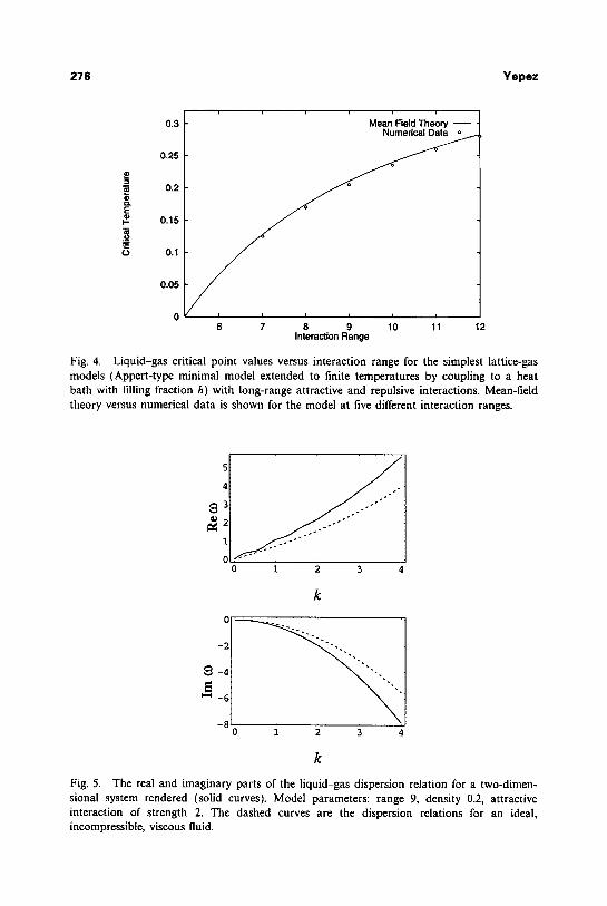
Figure 3 shows liquid-gas coexistence curves for this lattice-gas model at three different interaction ranges: r = 7 , 9, and III. Both the mean-field- theory calculation and the exact numerical data are presented. The comparison of the theory to the numerical simulation is in good agreement. In the Boltzmann limit, the probability of a long-range interaction goes as ~,2= d2( 1 -d)- ' . It is expected that this estimate, which neglects all particle correlations, would suffer the most at low densities where the mean free path between local collisions becomes comparable to the range of the nonlocal interactions. This may account for the deviations that are observed at low densities. The mean-field predictions of the critical point are also in quite good agreement with the numerically obtained values. Figure 4 shows the mean-field calculation and exact numerical data taken at five different interaction ranges: r = 7 through 1 ll. The calculated value of h c is slightly higher than the measured value for all cases, indicating a systematic deviation.

For the liquid-gas system, the dispersion relation (85) reduces to

m = +k 1 + -do(1 - d o ) ( 1 - 2 d o ) De(h ) C s - -

1/2 . vok2 x ( r , , k ) -W2 jo/2(r~,k) - t 2c--~, (100)

Figure 5 shows the real and imaginary parts of the liquid-gas dispersion curve for a two-dimensional system with a density of d--0.20 and momentum exchanges of tip-- - 2 m c over a range of r = 9/. Also shown for comparison purposes are the dispersion curves for an ideal, viscous fluid. In a long-range lattice gas, since the kinematic shear viscosity is dependent on


0 25 l

0.2

0.15 o.

0.1 [.-,

0 . 0 5

p = 3 d - 21 d^2(1-d)^2 (l-2h)

i Supercritical :Phase

i /e=itical Point ~ ~

. Li~id

0.i 0.2 0.3 0.4 0.5

Density

p=3d-27d^2(l-d)^2(l-2h)

r=7

0.25

0.2

~0.15

0.1

[-'0.05

0.i 0.2 0.3 0.4 0.5

Density

p = 3 d - 33 d^2(l-d)^2 (l-2h)

r=9

0.25

~ 0 . 2

~0.i!

0.05

0.i 0.2 0.3 0.4 0.5 0.6

Density

r=ll

Fig. 3. Liquid-gas coexistence curves for the simplest lattice-gas models (Appert-type minimal model extended %0 finite temperatures by coupling to a heat bath with filling fraction h) with long-range attractive and repulsive interactions. Mean-field theory versus numerical data is shown for the model at three different interaction ranges.

276 Y e p e z

,= g

: , = c o

0.3

0.25

0.2

0.15

0.1

0.05

0

, , , , ,

Mean Field Theory -- - Numerical Data *

I

i i i i i i

6 7 8 9 10 11 12 Interaction Range

Fig. 4. Liquid-gas critical point values versus interaction range for the simplest lattice-gas models (Appert-type minimal model extended to finite temperatures by coupling to a heat bath with filling fraction h) with long-range attractive and repulsive interactions. Mean-field theory versus numerical data is shown for the model at five different interaction ranges.

3 =; ==

o

-2

~-w -6

-8

0 1 2 3

k

0 1 2 3

k

Fig. 5. The real and imaginary parts of the liquid-gas dispersion relation for a two-dimensional system rendered (solid curves). Model parameters: range 9, density 0.2, attractive interaction of strength 2. The dashed curves are the dispersion relations for an ideal, incompressible, viscous fluid.

Lat t ice -Gas Crysta l l i za t ion 2 7 7

~>

30

25

20

15

10

5

0

i , , , , , ,

dp=2 (3 scans) * dp=l,2 (9 scans) +

dp=sqrt(3) (6 scans) a , / dp=l,sqrt(3),2 (15 scans) • / .

dp=l,sqrt(3),2 & rest particle (15 scans) ~ / . . " 0.096 rA2/z-~ ,: 0.294 rA~2 " .:i: . . . . . 0.116/~;~ ...... ..., 0.3j56.rA2 .-.:.:'

i g rA2 . . .

...-" g..."

...... ".~ ..... . ....... i-'J ......... "

..... -.-j ....... . ....... -.:~ .......

. . . . . . . . :: . . . . . . . . . .~ :~. . t~. - : : : : :z ; ' ' ' : " . . . . . . "J:"~" =

1 2 3 4 5 6 7 8 Interaction Range

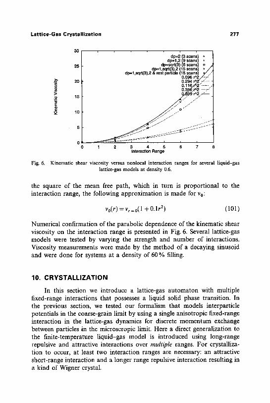
Fig. 6. K i n e m a t i c s h e a r v i scos i ty ve r sus n o n l o c a l i n t e r a c t i o n r a n g e s for severa l l i q u i d - g a s

l a t t i ce -gas m o d e l s a t dens i ty 0.6.

the square of the mean free path, which in turn is proportional to the interaction range, the following approximation is made for %:

v0(r) = Vr=o( 1 + 0.1r 2) (lO1)

Numerical confirmation of the parabolic dependence of the kinematic shear viscosity on the interaction range is presented in Fig. 6. Several lattice-gas models were tested by varying the strength and number of interactions. Viscosity measurements were made by the method of a decaying sinusoid and were done for systems at a density of 60 % filling.

10. CRYSTALLIZATION

In this section we introduce a lattice-gas automaton with multiple fixed-range interactions that possesses a liquid-solid phase transition. In the previous section, we tested our formalism that models interparticle potentials in the coarse-grain limit by using a single anisotropic fixed-range interaction in the lattice-gas dynamics for discrete momentum exchange between particles in the microscropic limit. Here a direct generalization to the finite-temperature liquid-gas model is introduced using long-range repulsive and attractive interactions over multiple ranges. For crystallization to occur, at least two interaction ranges are necessary: an attractive short-range interaction and a longer range repulsive interaction resulting in a kind of Wigner crystal.

278 Yepez

10.1. New Way for Molecular Dynamics Modeling

To model a more realistic crystal, that is, one that can undergo rigid-body motion such as rotation and that can have well-defined edges or surfaces, more then two interaction ranges are required. Usually four to eight interaction ranges are used to produce a Lennard-Jones-type molecular potential.

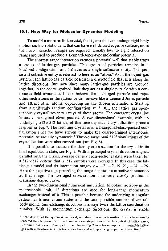
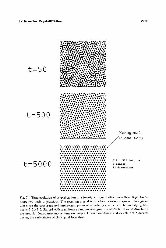
The shortest range interaction creates a potential well that stably traps a group of lattice-gas particles. This group of particles remains in a localized configuration and behaves as a single collective entity. This per- sistent collective entity is referred to here as an "atom." As in the l iquid-gas system, each lattice-gas particle possesses a discrete field that acts along the lattice directions. But now since many lattice-gas particles are grouped together, in the coarse-grained limit they act as a single particle with a con- tinuous field around it. It can behave like a charged particle and repel other such a toms in the system or can behave like a Lennard-Jones particle and at tract other atoms, depending on the chosen interactions. Starting from a uniformly random configuration at d = 0.1, the lattice gas spon- taneously crystallizes into arrays of these atoms. The emergent crystalline lattice is hexagonal close packed. A two-dimensional example, with an underlying 512 x 512 lattice, of this t ime-dependent crystallization process is given in Fig. 7. The resulting crystal is in a hexagonal-close-packed configuration since we have striven to make the coarse-grained interatornic potential be radially symmetric. 3 Three-dimensional 5123 simulations of the crystallization were also carried out (see Fig. 8).

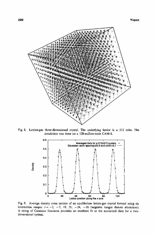
It is possible to measure the density cross section for the crystal in its final equilibrium state; see Fig. 9. With a principal crystal direction aligned parallel with the x axis, average density cross-sectional data were taken for a 512 x 512 system; that is, 512 samples were averaged. In this case, the lattice-gas model had six interaction ranges: r = - 2 , - 7 , 19, 21, - 2 4 , - 2 6 . Here the negative sign preceding the range denotes an atractive interaction at that range. The averaged cross-section da ta very closely produce a Gaussian-shaped curve.

In the two-dimensional numerical simulation, to obtain isotropy in the macroscopic limit, 12 directions are used for long-range m o m e n t u m exchanges instead of 6. This is possible because the underlying tr iangular lattice has 6 m o m e n t u m states and the total possible number of central- body momen tum exchange directions is always twice the lattice coordination number. With 12 m o m e n t u m exchange directions, the crystal is stable

If the density of the system is increased, one does observe a transition from a hexagonally ordered bubble phase to ordered and random stripe phases. In the context of lattice gases, Rothman has shown some pictures similar to Fig. 7 in a two-component immiscible lattice gas with a short-range attractive interaction and a longer range repulsive interaction, m~


t=50

t=500

t=5000

l o.:....,',:,* e-,'o, ~,;o,

[~ ,, 4, *_e �9 �9 e ' e r ' . � 9 ~ , '~*'e �9 ~.e, �9 e

~ t t l I ' t l t ' I i l l t l I t l I O ~ O ~ l R i ~ B Q � 9 I l l l O I l l l . ~ l ' * t i ~ l l l l

m m 4 o o o e ~ t . * e ~ 4 0 o o o e o l

s * Q i o S a 6 o ~ o o Q e l ~ o t o e q g o g D J e o u e e o 4 6 * ~ ~ 6 6 B 6

V.'AV.V.'.~V.'A*A'.'.V~ '.V:A~VAV.V/,~V.V:

~t~'22222.tt'22.ttt"C22

Hexagonal //Close Pack

/

512 x 512 Lattice

6 ranges

12 directions

Fig. 7. Time evolution of crystallization in a two-dimensional lattice gas with multiple fixed- range two-body interactions The resulting crystal is in a hexagonal-close-packed configuration since the coarse-grained interatomic potential is radially symmetric. The underlying lattice is 512 x 512. Started with a uniformly random configuration at d = 0.1. Twelve directions are used for long-range momentum exchanges. Grain boundaries and defects are observed during the early stages of the crystal formation.

280 Yepez

Fig. 8. Lattice-gas three-dimensional crystal. The underlying lattice is a 512 cube. The simulation was done on a 128-million-node CAM-8.

0 . 6

0.5

0.4

0.3

0.2

0.1

0 0

oJ a

Averaged data for a 512x512 system o Gaussian: atom spacing=25.6 and width=3.7 ......

i '! : b

q

i ~ ,

, j i i

20 40 60 80 100 Lattice position along the x-axis

Fig. 9. Average density cross section of an equilibrium lattice-gas crystal formed using six interaction ranges: r = - 2 , - 7 , 19, 21, - 2 4 , - 2 6 (negative ranges denote attraction). A string of Gaussian functions provides an excellent fit to the numerical data for a two- dimensional system.


0.2

3 ~0.i

0

y;/ 0 0.i 0.2

k

0.01

C

3 -o.oz

- 0 . 0 2

- 0 . 0 3

0 0 . 1 0 . 2

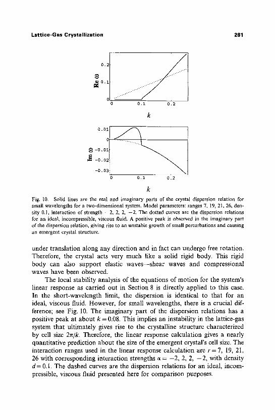
Fig. 10. Solid lines are the real and imaginary parts of the crystal dispersion relation for small wavelengths for a two-dimensional system. Model parameters: ranges 7, 19, 21, 26, density 0.1, interaction of strength -2, 2, 2, -2. The dotted curves are the dispersion relations for an ideal, incompressible, viscous fluid. A positive peak is observed in the imaginary part of the dispersion relation, giving rise to an unstable growth of small perturbations and causing an emergent crystal structure.

under translation along any direction and in fact can undergo free rotation. Therefore, the crystal acts very much like a solid rigid body. This rigid body can also support elastic waves--shear waves and compressional waves have been observed.

The local stability analysis of the equations of mot ion for the system's linear response as carried out in Section 8 is directly applied to this case. In the short-wavelength limit, the dispersion is identical to that for an ideal, viscous fluid. However, for small wavelengths, there is a crucial difference; see Fig. 10. The imaginary part of the dispersion relations has a positive peak at about k--0 .08. This implies an instability in the lattice-gas system that ultimately gives rise to the crystalline structure characterized by cell size 2n/k. Therefore, the linear response calculation gives a nearly quantitative prediction about the size of the emergent crystal's cell size. The interaction ranges used in the linear response calculation are r = 7, 19, 21, 26 with corresponding interaction strengths 0~-- - 2 , 2, 2, - 2 , with density d--0.1. The dashed curves are the dispersion relations for an ideal, incompressible, viscous fluid presented here for comparison purposes.

282 Yepez

10.2. The Crystal Reconfiguration Process

An expected phenomenon that occurs in the early stages of the crystal formation is the emergence of grain boundaries and defects. Over time, given the inherent fluctuations of the lattice-gas dynamics, the crystal undergoes an annealing process that removes the defects and eventually produces a prefect crystal. In the two-dimensional case with a radially symmetric coarse-grained potential, the hexagonal-close-packed crystal structure emerges as just mentioned. Defect pairs with five and seven neighbors are observed.

An unexpected phenomenon that occurs in the exact simulation is the process by which a defect is removed. To describe this process, consider, for example, an atom with five neighbors. It may persist in such a frustrated situation for some time. Yet what eventually occurs is that the lattice structure near this defect begins to fluctuate--"tremors" in the crystal structure are observed. That is, the other atoms in the immediate vicinity of the defect begin to vibrate about their metastable positions. The magnitude of the fluctuations increases over time. In fact, the magnitude of the fluctuations appears to grow and one may even say that the temperature of the local crystalline structure appears to rise. When a high enough local temperature of this sort is reached, the microscopic dynamics suddenly reconfigures a cluster of the atoms and the defect vanishes. The reconfiguration of the atoms usually entails a small local rotation of a cluster of atoms surrounding the defect site.

One way to characterize the fluctuations that occur in the system leading to the rather sudden reconfiguration of a cluster of atoms is to compare the state of the system at one time t to the state at some later time t + T by computing a Hamming length. In discrete models, such as the Ising model or a Hopfield neutral network, a Hamming length is well defined. In a lattice gas, one can also define a Hamming length hr and in particular we do so in the coarse-grained limit. That is, a block average of the lattice-gas number variables is taken to determine a density field p(x). The Hamming length is calculated by summing over all points of the density field as follows:

ht=~ O(Ip(x, t+ T)--p(x, t ) l - e ) (102) x

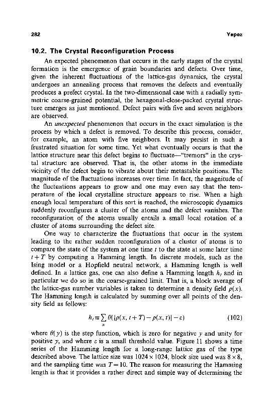
where 0(y) is the step function, which is zero for negative y and unity for positive y, and where e is a small threshold value. Figure 11 shows a time series of the Hamming length for a long-range lattice gas of the type described above. The lattice size was 1024 x 1024, block size used was 8 • 8, and the sampling time was T = 10. The reason for measuring the Hamming length is that it provides a rather direct and simple way of determining the


Fig. 11. Hamming length time-series data for a long-range lattice-gas with eight different ranges. The Hamming length corresponds to the size of a reconfiguration event due to inherent fluctuation of the underlying lattice gas. Data taken for a 1024 x 1024 simulation using 8 x 8 block averaging and a sample time T = 10.

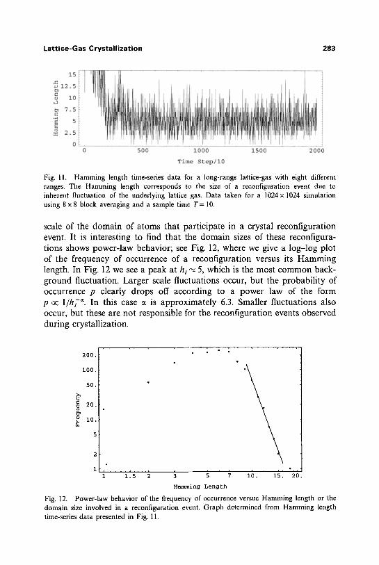
scale of the domain of atoms that participate in a crystal reconfiguration event. It is interesting to find that the domain sizes of these reconfigura- tions shows power-law behavior; see Fig. 12, where we give a log-log plot of the frequency of occurrence of a reconfiguration versus its Hamming length, In Fig. 12 we see a peak at h~ -~ 5, which is the most common back- ground fluctuation. Larger scale fluctuations occur, but the probability of occurrence p clearly drops off according to a power law of the form p oc l /h7 ~. In this case 0c is approximately 6.3. Smaller fluctuations also occur, but these are not responsible for the reconflguration events observed during crystallization.

i00. I

50.

2 0 .

1 0 . t,,

200.

1 1.5 2 3 5 7 i0. 15. 20.

Hamming Length

Fig. 12. Power-law behavior of the frequency of occurrence versue Hamming length or the domain size involved in a reconfiguration event. Graph determined from Hamming length time-series data presented in Fig. 11.

284 Yepez

11. CONCLUSION

We have presented a mean-field theory of lattice gases with long-range interactions. We have focused on central-body interactions that are mediated by momentum exchange events between remote spatial sites and have used this type of interaction to model two types of physical systems: (a) a finite-temperature liquid-gas dynamical system; and (b) a solid-state molecular dynamical system. The latter lattice-gas model is very compelling and is the most important result of this paper. This lattice-gas model of a crystallographic solid body offers an alternative to traditional molecular dynamics modeling. The dynamical behavior of the lattice-gas solid is exactly computed, in that there is exact conservation of mass, momentum, and energy. A solid phase is self-consistently produced through the collective and nonlinear behavior of billions of lattice-gas particles as they inter- act via local collisions and long-range interactions. A linear stability analysis is presented that predicts the formation of "atoms" of a charac- teristic interatomic spacing, each atom itself occupying a finite volume and composed of thousands of lattice-gas particles. Therefore, the atom, is not a point particle, but is distributed over several lattice sites and is stable in a self-consistent way. Each atom possesses a Lenord-Jones-type potential in the coarse-grained limit. The mass of an atom as well as its field are both manifestations of the spatial distribution of lattice-gas particles. A lattice- gas particle is interpreted as an informational token that composes only a small piece of the atom and contributes to a small piece of its field. We have observed an annealing process where defects are removed from the crystal where there is a succession of localized vibrations that continually build to the point where a cluster of molecules around the defect can eventually undergo a reconfiguration. Fluctuations within the crystal structure exhibit power-law behavior.

APPENDIX A. LATTICE MULTIPOLE T H E O R E M

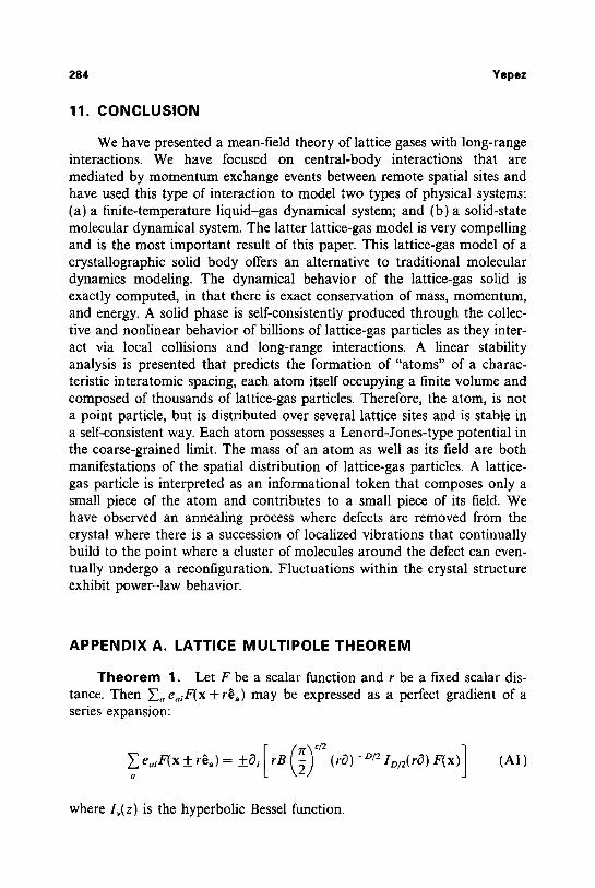
Theorem 1. Let F be a scalar function and r be a fixed scalar distance. Then Za eaiF(x +_r~a) may be expressed as a perfect gradient of a series expansion:

~o e~,F(x+_r~a)= +_O,[rB(2)~/2(rO)-D/2ID/2(rO)F(x) 1 (A1)

where I,.(z) is the hyperbolic Bessel function.


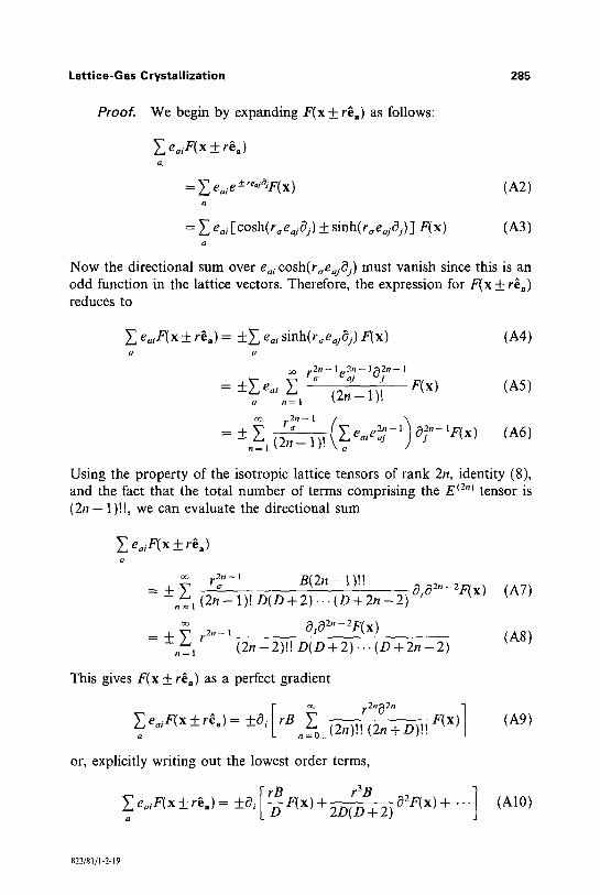
Proof. We begin by expanding F(x 4- r~.) as follows:

~" e.iF(x 4- r~.) a

2 +rea'OJ e~ie- 'J F(x) (A2) Q

= ~ e.;[cosh(r.e./O/) + sinh(r~e.jO:)] F(x) (A3) a

Now the directional sum over e~; cosh(r~e.jO/) must vanish since this is an odd function in the lattice vectors. Therefore, the expression for F(x 4- rg.) reduces to

~. eaiF(x +__ r~8) = -t-y" e.i sinh(r~eo/Oi) F(x) (A4) a (.i

~,, 2 n - 1 2 n - lc~2n- I = ++-~ eai r~ e~ -: F(x) (A5)

. . . . 1 ( 2 n - 1 )!

" ' (z ) r . 2 . - , O~,,-iF(x) (A6) = 4- (2nn= i)! e"'e~s

Using the property of the isotropic lattice tensors of rank 2n, identity (8), and the fact that the total number of terms comprising the E (2") tensor is ( 2 n - 1)!!, we can evaluate the directional sum

eoiF(x +_ r~.) Q

o~ 2,,-1 B ( 2 n - 1) vT - +-.~'l r~ "" O;O2"-'-F(x) (A7) - = ( ~ n ~ l ) ! O ( D + 2 ) . . . ( D + 2 n - 2 )

---~ ~ ~ /.2n--1 0i 02,'-2F(X) (A8) .=1 ( 2 n - 2 ) ! ! D ( D + 2 ) . . . ( D + 2 n - 2 )

This gives F(x 4-r~.) as a perfect gradient

Z eaiF(x 4-r~.a) = +0 i rB . . . . o... (2n)!! (2n + D)!! F(x) (A9)

or, explicitly writing out the lowest order terms,

[rB rSB ] . e.iF(x __. r~.) = _ +0i ~ - F(x) 4 2D(D + 2) O2F(x) + "" (A10)

822/81/I-2-19

286 Yepez

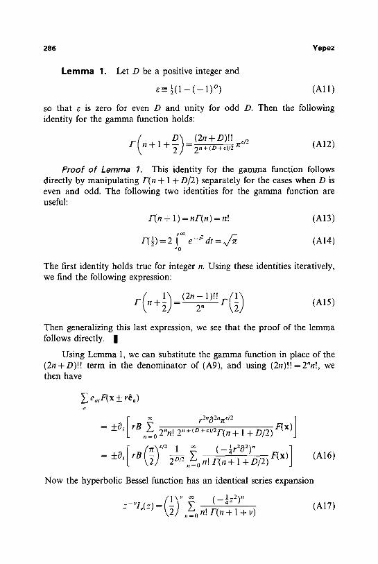
Lemma 1. Let D be a positive integer and

e - � 8 9 ~ (Al l )

so that e is zero for even D and unity for odd D. Then the following identity for the gamma function holds:

( D) (2n+D),! /2 (A12) F 11+ 1 + --2,,+(0+~)/2

Proof o f l_emma 7. This identity for the gamma function follows directly by manipulating F(n + 1 + 1)/2) separately for the cases when D is even and odd. The following two identities for the gamma function are useful:

F(n + 1) = nF(n) = n! (A13)

r(1) = 2 e-'2dt=.v/-~ (AI4)

The first identity holds true for integer n. Using these identities iteratively, we find the following expression:

Then generalizing this last expression, we see that the proof of the lemma follows directly, l

Using Lemma 1, we can substitute the gamma function in place of the (2n +D)!! term in the denominator of (A9), and using (217)!! =2"n!, we then have

e.iF( x +_ r6.)

= +8i rB 2,,+Io+~v2F( n F(x) ,,=o 2"n! + 1 +D/2)

= +O, rB \2J 2 ~ n! F(n + 1 + D/2) F(x) (AI6)

Now the hyperbolic Bessel function has an identical series expansion

- - " - ( - ~ : ) (A17) -~ L(-') = n! F(n + 1 + v) t l ~ 0

Lattice-Gas Crystallization 2 8 7

Therefore, taking v = D/2 and considering z to be a differential operator, z---, r0, we find that (A16) becomes

~, %iF(x +__ r~.) = +rO, B a

which completes the proof of Theorem 1.

l (rO)-~ lo/2(rO) F(x)]

I

(A18)

APPENDIX B. NUMERICAL IMPLEMENTATION OF THE LONG-RANGE TWO-BODY INTERACTIONS

A simple computational scheme is employed that allows all the dynamics to be computed in parallel with two additional bits of local site data, for outgoing and incoming messengers, regardless of the number of long-range neighbors. The computational scheme is an efficient decomposi- tion of a lattice gas with many neighbors. It is conceptually similar to the idea of virtual intermediate particle momentum exchanges that is well known in particle physics. All two-body interactions along a particular direction define a spatial partition that is updated in parallel. Random per- mutation through the partitions is sufficient to recover the necessary isotropy as long as enough momentum exchange directions are used.

An interparticle potential V ( x - x ' ) acts on particles spatially separated by a fixed distance x - x ' = r. An effective interparticle force is caused by a nonlocal exchange of momentum. Momentum conservation is violated locally, yet it is exactly conserved in the global dynamics.

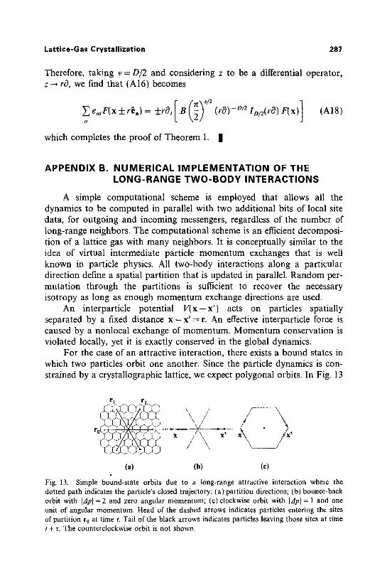
For the case of an attractive interaction, there exists a bound states in which two particles orbit one another. Since the particle dynamics is constrained by a crystallographic lattice, we expect polygonal orbits. In Fig. 13

rl r 2

t .[ ~.\]~"YZ.(Y / \ / / .'I "~ "].X'I/T. "l: ~i~ 3 ",/

r, [ "1" "V'"r "l'" T "r ~L--- ~ . .

T IZr.i 3Xf :[ T / \ CL_cj- ?C-~].C.C] / , ',, /

(a) (b) (c)

Fig. 13. Simple bound-state orbits due to a long-range attractive interaction where the dotted path indicates the particle's closed trajectory: (a) partition directions; (b) bounce-back orbit with IApl = 2 and zero angular momentum; (c) clockwise orbit with 13pl = 1 and one unit of angular momentum. Head of the dashed arrows indicates particles entering the sites of partition r0 at time t. Tail of the black arrows indicates particles leaving those sites at time t + r. The counterclockwise orbit is not shown.

288 Yepez

we depict two such orbits for a hexagonal lattice gas. The range of the interaction is r. Two-body single-range attractive interactions are depicted in Figs. 13b and 13c, the bounce-back and clockwise orbits, respectively. Momentum exchanges occur along the principal directions. The interaction potential is not spherically symmetric, but has an angular anisotropy. In general, it acts only on a finite number of points on a shell of radius r/2. The number of lattice partitions necessary per site is half the lattice coordination number, since two particles lie on a line. Though microscopically the potential is anisotropic, in the continuum limit obtained after coarse- grain averaging, numerical simulation indicates isotropy is recovered.

B1. Simple Example: Bounce-Back Orbit

A long-range lattice gas of the type we are considering still possesses the usual local dynamics of a hydrodynamic lattice gas. To extend the local lattice-gas update rules to include long-range interactions, we use two additional bits of local site data. This will allow us to implement a long-range interaction using strictly local updating and therefore our algorithm will still be parallelizable just like a usual local lattice gas. The two additional bits will denote the occupation numbers of messenger particles, or "photons." The idea of using messenger particles was introduced by Appert et al. ~ ~ We have two types of messenger states, to represent incoming and outgoing conditions, and we denote the messengers as tPt and qJr-

Now for the simplest long-range lattice-gas model, we therefore use eight bits of local site data. Since long-range interactions occur between remote spatial sites, say x and x', the messenger particles will travel either parallel or antiparallel to the vector r = x - x'. All pairs of sites throughout the entire space that are separated by vector r can therefore all be updated in parallel. We refer to an update step of all pairs of two-body interactions along direction r as a parti t ion, denoted by F,.. All possible two-body interaction pairs are then computed by performing all possible partitions of the space. So it requires many scans for the space to perform a single long- range interaction step.

In our two-dimensional example using a triangular lattice, there are three possible partitions. The number of partitions is never smaller than half the lattice coordination number. In the two-dimensional case, the simplest long-range lattice-gas algorithm, though perhaps not the most efficient algorithm, is to use three sequential scans of the space, each scan performing the updating necessary for a single partition (see Fig. 13a). Often, depending on the complexity of the long-range interactions and the dimensionality of the lattice, it is possible to perform s imultaneous updating of multiple partitions. This of course is more desirable, yet causes more

Lat t ice-Gas Crystal l izat ion

Table I. Lat t ice Vec tor Components

a x Component y Component

0 -1 0 1 - " , f i n 2 �89 x/~/2 3 1 0 4 ~ _ --V/3/2 5 -~ - , , i l l2

289

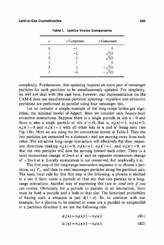
complexity. Furthermore, this updating requires an extra pair of messenger particles for each partition to be simultaneously updated. For simplicity, we will not deal with this case here; however, our implementation on the CAM-8 does use simultaneous partition updating--repulsive and attractive partitions are performed in parallel using four messenger bits.

Let us consider a simple example of the long-range lattice-gas algorithm, the minimal model of Appert. Here we consider only bounce-back attractive interactions. Suppose there is a single particle at site x = 0 and there is also a single particle at site x' =r] ; that is, no(X)= 1, n3(x)=0, no(X')=0 and n3(x ' )= 1 with all other bits at x and x' being zero (see Fig. 13b). Here we are using the bit convention shown in Table I. Then the two particles are separated by a distance r and are moving away from each other. The attractive long-range interaction will effectively flip their respec- tive directions making no(x)=0 , n 3 ( x ) = l , no(X')= 1, and n3(x ' )=0 , so that the two particles will now be moving toward each other. There is a local momentum change of 2mc] at x' and an opposite momentum change of - 2 m c l at x. Locally momentum is not conserved, but nonlocally it is.

The first step of the long-range interaction sequence is to choose a partition, say F,, and then to emit messenger particles along the partition axis. The basic local rule for this first step is the following: a photon is emitted at a site if there exists a particle at that site that can partake in a long- range interaction. Another way of expressing this rule is: send only i f you can receive. Obviously, for a particle to partake in an interaction, there must be both a particle and a hole at that site. The factorized probability of having such a situation is just d ( 1 - d ) . So, to continue with our example, for a l~hoton to be emitted at some site x parallel or antiparallel to a partition direction i, we use the following rule:

~b ~(x) = no(x)( 1 - n3(x)) (B1)

~t/(X) = n3(X)(1 -- no(X)) (B2)

290 Yepez

Note that according to this local rule, only one photon can be created at a site, and consequently we eliminate the possibility of a long-range interaction, say of range 2r, mediated through a doubly occupied site. The impor tant consequence of the emission step is that for two sites separated by the interaction distance r, if both sites send photons, both will necessarily receive them, which strictly enforces nonlocal m o m e n t u m conservation. Give and ye shall receive (provided yours is received). Letting ~ - ~ . and 4 - . - O / , in general we can write the emission step of the minimal interaction as

@,(x) = n _~(x)( 1 - n , (x)) (B3)

where a = 0, 1, 2 covers all the partitions. After the emission step follows a long-range kick of the messenger bits.

In the simple example, all photons ~,~ are kicked along - r l and all photons ~,, are kicked along rl. In general, for the long-range kick we have

~,'~(x + rS~) = ~%(x) (B4)

Finally, we have the absorpt ion step of the long-range interaction sequence. Here the local particle m o m e n t u m state is updated as the particles flip their directions, in our example

n~(x) = n3(x ) + ifl~(x) no(x)(1 --n3(x)) -- ~'r(X) n3(x)(1 --no(x)) (BS)

n~(x) = no(x) + ~k'r(x) n3(x)( 1 - no(x)) -- ~ ( x ) no(x)(1 -- n3(x)) (B6)

Moreover , in this step all the messenger bits are set to zero throughout the entire space. For any direction, the local absorpt ion rule could more simply be written as

n ' (x ) = n~(x) + q/_~(x) ff~(x) -- ~'~(x) ~b _a(x) (B7)

Substituting in (B3) and (B4) into (B7), we have a single Boolean expression in terms of number variables for a single long-range interaction step for part i t ion F , as follows:

n'a(X) = no(X)

+ n . (x + r~.)( 1 -- n _ . (x + r~.)) n_ . (x ) ( 1 - n,,(x))

- n _ ~ ( x - - rOa)(1 - n . (x - r~.)) n~(x)(1 - n ,,(x)) (B8)

For convenience we define a long-range collision opera tor P~ as follows:

Pa(x,x+r8.)=t~_~(x+r~,,)~a(x)=~k'_~(x)~.(x) (B9)

Lattice-Gas Crystallization

Table Ii. Long-Range Interaction Sequence

291

Events na(x) zt(x ) z,(x) no(x') zt(x') z,(x')

Initial 100000 0 0 000100 0 0 Emit 100000 0 1 000100 1 0 Kick 100000 1 0 000100 0 1 Absorb 000100 0 0 100000 0 0

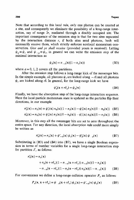
so that we may write

n',,(x) = n~(x) + P~(x, x + r~ ) - P_a(x, x - r~a) (B10)

The state data for the simple example we have been considering are given in Table II, which represents all the steps of a long-range interaction sequence for a partition along the x axis.

B2. Another Example: Clockwise Orbit

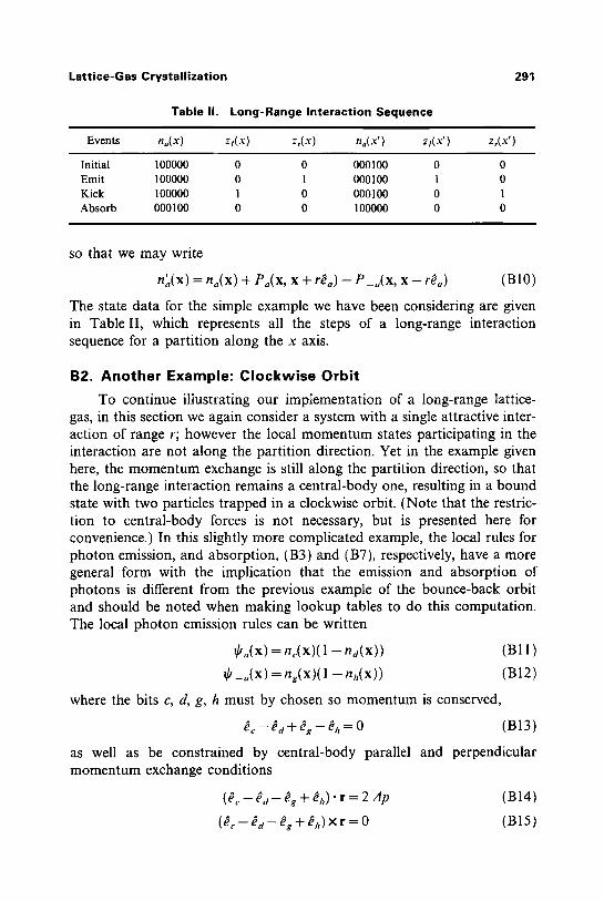
To continue illustrating our implementation of a long-range lattice- gas, in this section we again consider a system with a single attractive interaction of range r; however the local momentum states participating in the interaction are not along the partition direction. Yet in the example given here, the momentum exchange is still along the partition direction, so that the long-range interaction remains a central-body one, resulting in a bound state with two particles trapped in a clockwise orbit. (Note that the restric- tion to central-body forces is not necessary, but is presented here for convenience.) In this slightly more complicated example, the local rules for photon emission, and absorption, (B3) and (BT), respectively, have a more general form with the implication that the emission and absorption of photons is different from the previous example of the bounce-back orbit and should be noted when making lookup tables to do this computation. The local photon emission rules can be written

~a(x) = n~(x)(l - ha(X)) (BI 1 )

_a(x) = ng(x)(1 --n/,(x)) (B12)

where the bits c, d, g, h must by chosen so momentum is conserved,

ec-- ea + es-- eh = 0 (B13)

as well as be constrained by central-body parallel and perpendicular momentum exchange conditions

(~c - ~ a - ~g + ~h)" r = 2 dp (B14)

(~ - - ~ d - - ~g + ~J,) x r = 0 ( B 1 5 )

292 Yepez

where zlp is the momentum change per site due to the long-range interaction. In (B 11) and (BI2) the difference from our previous example of the bounce-back orbit is the possibility of having two photons emitted at a single site.

To be explicit, for the two-dimensional triangular lattice, we can satisfy (B13)-(B15) by choosing the indices c, d, g, h as follows:

c = a - 2 (B16)

d = a - 1 (B17)

g = - c (B18)

h = - d (B19)

An example of this choice of indices is illustrated in Fig. 13c. Then the emission rule, (B l l ) and (B12), is simply

~b~(x) = n~_2(x)( 1 - n~_ l(x)) (B20)

Since the kicking of the photons is the same in this example as in the previous one, (B4) still holds,

~',,(x + r~,,) = ~ , , ( x )

By reexpressing (B7) more generally, we can write a local absorption rule

n'o(x) = n,,(x) + ~b'(, + i)(x) ~ba + l(x) - ~,'~_ l(x) ~b_c~_ l)(x) (B21)

or more elegantly

n'o(x)=n,,(x)+P~+l(x,x+rO~+j)--P_o+l(x,x--rdo_l) (B22)

Substituting in (B20) and (B4) into (B21) and after some manipulation of the indices, we have a single Boolean expression in terms of number

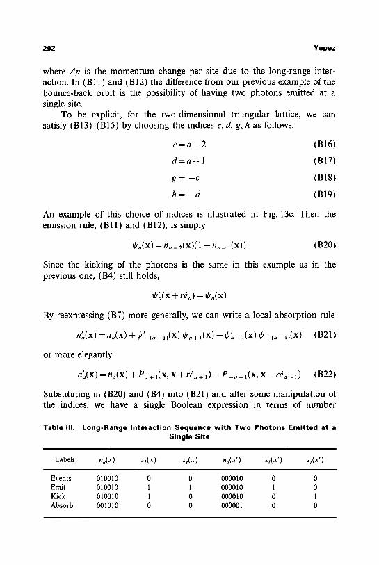
Table III. L o n g - R a n g e Interaction Sequence with Two Photons Emitted a t a Single Site

Labels no(x) zt(x) zr(x) na(x') gl(X') gr(X')

Events 010010 0 0 000010 0 0 Emit 010010 1 1 000010 1 0 Kick 010010 1 0 000010 0 1 Absorb 001010 0 0 000001 0 0

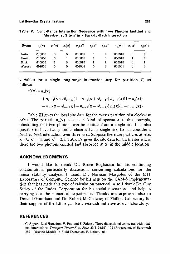
Lat t ice-Gas Crys ta l l i za t ion 293

Table IV. Long-Range Interaction Sequence with T w o Photons Emitted and Absorbed at Si te x ' in a Back- to -Back Interaction

Events n.(x) zt(x) zr(x) no(x') zl(x') zr(x') na(x") zt(x") Zr(Xt')

Initial 010000 0 0 010010 0 0 000010 0 0 Emit 010000 0 1 010010 1 1 000010 1 0 Kick 010000 1 0 010010 1 1 000010 0 1 Absorb 001000 0 0 001001 0 0 000001 0 0

variables for a single long-range interaction step for partit ion Fr as follows:

n'o(x) =no(x)

+ na +2(x -I- rda+ 1)(1 -- n _ , ( x + rd,+ l)) 17,,_ l(x)(1 - na(x))

- n _ , ( x - r ~ o _ t)(1 - n a _ 2 ( x - rdo_ 1)) na(x)(1 - n~+ l(x))

Table I I I gives the local site data for the x-axis partit ion of a clockwise orbit. The particle na(x ) acts as a kind of spectator is this example, illustrating that two photons can be emitted from a single site. It is also possible to have two photons absorbed at a single site. Let us consider a back- to-back interaction over three sites. Suppose there are particles at sites x = 0, x ' = ri, and x" = 2ri. Table IV gives the site data for these sites where there are two photons emitted and absorbed at x ' in the middle location.

A C K N O W L E D G M E N T S

I would like to thank Dr. Bruce Boghosian for his continuing collaboration, particularly discussions concerning calculations for the linear stability analysis. I thank Dr. Norman Margolus of the MIT Labora tory of Computer Science for his help on the CAM-8 implementation that has made this type of calculation practical. Also I thank Dr. Guy Seeley of the Radex Corporat ion for his useful discussions and help in carrying out the numerical experiments. Thanks are expressed also to Donald Gran tham and Dr. Robert McClatchey of Phillips Labora tory for their support of the lattice-gas basic research initiative at our laboratory.

REFERENCES

1. C. Appert, D. d'Humi~res, V. Pot, and S. Zaleski, Three-dimensional lattice gas with minimal interactions, Transport Theory Stat. Phys. 23( 1-3 ): 107-122 ( Proceedings of Euromech 287--Discrete Models in Fluid Dynamics, P. Nelson, ed.).

294 Yepez

2. C. Appert and S. Zaleski, Lattice gas with a liquid-gas transition, Phys. Rev. Lett. 64:1-4 (1990).

3. P. L. Bhatnagar, E. P. Gross, and M. Krook, A model for collision processes in gases, i. Small amplitude processes in charged and neutral one-component systems, Phys. Reo. 94(3):511-525 (1954).

4. Hudong Chen, Shiyi Chen, and W. H. Mattaeus, Recovery of the Navier-Stokes equations using a lattice-gas Boltzmann method, Phys. Rev. A 45(8):R5339-R5342 (1992).

5. Shiyi Chen, Hudong Chen, D. Martinez, and W. Matthaeus, Lattice Boltzmann model for simulation of magnetohydrodynamics, Phys. Rev. Lett. 67(27):3776-3779 (1991).

6. U. Frisch, D. d'Humi6res, B. Hasslacher, P. Lallemand, Y. Pomeau, and J.-P. Rivet, Lattice gas hydrodynamics in two and three dimensions, Complex Systems 1:649-707 (1987).

7. M. H6non, Viscosity of a lattice gas, in Lattice Gas Methods for Partial Differential Equations, G. D. Doolean, ed. (Addison-Wesley, Reading, Massachusetts, 1990).

8. L. P. Kadanoff and J. Swift, Transport coefficients near the critical point: A master- equation approach, Phys. Rev. 165( 1 ):310-322 (1967).

9. L. D. Landau and E. M. Lifshitz, Fluid Mechanics, 2nd ed. (Pergamon Press, Oxford, 1987).

10. Y. H. Qian, D. d'Humi6res, and P. Lallemand, Lattice BGK models for Navier-Stokes equation, Europhys. Lett. 17(6bis):479-484 (1992).

11. D. H. Rothman, From ordered bubbles to random stripes--Pattern-formation in a hydrodynamic lattice-gas, J. Stat. Phys. 71(3--4):641-652 (1993).

12. Xiaowen Shan and Hudong Chen, Simulation of nonideal gases and liquid-gas phase transitions by the lattice Boltzmann equation, Phys. Rev. E 49(4):2941-2948 (1994).

13. S. Wolfram, Cellular automaton fluids t: Basic theory, J. Stat. Phys. 45(3/4):471-526 (1986).

14. J. Yepez, Lattice-gas dynamics on the cm-5 and cam-8, in Second Annual Technical bTter- change Symposium Proceedings (Phillips Laboratory, PL/XPP, 1993), Vol. I, p. 217.

15. J. Yepez, A reversible lattice-gas with long-range interactions coupled to a heat bath, in Proceedings of the Pattern Formation and Lattice-Gas Automata NATO Advanced Research H"orkshop, R. Kapral and A. Lawniczak, eds. (American Mathematical Society, Providence, Rhode Island, 1993).

Lattice-gas crystallization

Documents

Transcript of Lattice-gas crystallization