Investigation of non-equilibrium crystallization of mixed gas ...

HAL Id: tel-01665152https://tel.archives-ouvertes.fr/tel-01665152

Submitted on 15 Dec 2017

HAL is a multi-disciplinary open accessarchive for the deposit and dissemination of sci-entific research documents, whether they are pub-lished or not. The documents may come fromteaching and research institutions in France orabroad, or from public or private research centers.

L’archive ouverte pluridisciplinaire HAL, estdestinée au dépôt et à la diffusion de documentsscientifiques de niveau recherche, publiés ou non,émanant des établissements d’enseignement et derecherche français ou étrangers, des laboratoirespublics ou privés.

Investigation of non-equilibrium crystallization of mixedgas clathrates hydrates : an experimental study

compared to thermodynamic modeling with and withoutflash calculations

Quang-Du Le

To cite this version:Quang-Du Le. Investigation of non-equilibrium crystallization of mixed gas clathrates hydrates : anexperimental study compared to thermodynamic modeling with and without flash calculations. Other.Université de Lyon, 2016. English. �NNT : 2016LYSEM002�. �tel-01665152�

https://tel.archives-ouvertes.fr/tel-01665152

https://hal.archives-ouvertes.fr

NNT: 2016LYSEM002

THÈSE

présentée par

Quang-Du LE

pour obtenir le grade de

Docteur de l’École Nationale Supérieure des Mines de Saint-Étienne

Spécialité : Génie des Procédés

INVESTIGATION DE LA CRISTALLISATION HORS-ÉQUILIBRE

DES CLATHRATES HYDRATES DE GAZ MIXTES: UNE ÉTUDE

EXPÉRIMENTALE COMPARÉE À LA MODÉLISATION

THERMODYNAMIQUE AVEC ET SANS CALCULS FLASH

soutenue à Saint-Étienne, le 09 mars 2016

Membres du jury

Rapporteurs: Ryo OHMURA

Karine BALLERAT-BUSSEROLLES

Keio University, Yokohama, Japan

Université Blaise-Pascal, Ingénieure de

Recherche CNRS

Examinateurs: Eric CHASSEFIERE

Pierre DUCHET-SUCHAUX

Baptiste BOUILLOT

Jean-Michel HERRI

Université Paris-Sud

TOTAL SA, Paris

EMSE, Co-Encadrant

EMSE, Encadrant HDR

Invité: Freddy GARCIA TOTAL SA, Paris

Spécialités doctorales Responsables : Spécialités doctorales Responsables

SCIENCES ET GENIE DES MATERIAUX K. Wolski Directeur de recherche MATHEMATIQUES APPLIQUEES O. Roustant, Maître-assistant MECANIQUE ET INGENIERIE S. Drapier, professeur INFORMATIQUE O. Boissier, Professeur GENIE DES PROCEDES F. Gruy, Maître de recherche IMAGE, VISION, SIGNAL JC. Pinoli, Professeur SCIENCES DE LA TERRE B. Guy, Directeur de recherche GENIE INDUSTRIEL A. Dolgui, Professeur SCIENCES ET GENIE DE L’ENVIRONNEMENT D. Graillot, Directeur de recherche MICROELECTRONIQUE S. Dauzere Peres, Professeur

EMSE : Enseignants-chercheurs et chercheurs autorisés à diriger des thèses de doctorat (titulaires d’un doctorat d’État ou d’une HDR) ABSI Nabil CR Génie industriel CMP

AVRIL Stéphane PR2 Mécanique et ingénierie CIS

BALBO Flavien PR2 Informatique FAYOL

BASSEREAU Jean-François PR Sciences et génie des matériaux SMS

BATTAIA-GUSCHINSKAYA Olga CR Génie industriel FAYOL

BATTON-HUBERT Mireille PR2 Sciences et génie de l'environnement FAYOL

BERGER DOUCE Sandrine PR2 Sciences de gestion FAYOL

BIGOT Jean Pierre MR(DR2) Génie des Procédés SPIN

BILAL Essaid DR Sciences de la Terre SPIN

BLAYAC Sylvain MA(MDC) Microélectronique CMP

BOISSIER Olivier PR1 Informatique FAYOL

BONNEFOY Olivier MA(MDC) Génie des Procédés SPIN

BORBELY Andras MR(DR2) Sciences et génie des matériaux SMS

BOUCHER Xavier PR2 Génie Industriel FAYOL

BRODHAG Christian DR Sciences et génie de l'environnement FAYOL

BRUCHON Julien MA(MDC) Mécanique et ingénierie SMS

BURLAT Patrick PR1 Génie Industriel FAYOL

COURNIL Michel PR0 Génie des Procédés DIR

DAUZERE-PERES Stéphane PR1 Génie Industriel CMP

DEBAYLE Johan CR Image Vision Signal CIS

DELAFOSSE David PR0 Sciences et génie des matériaux SMS

DELORME Xavier MA(MDC) Génie industriel FAYOL

DESRAYAUD Christophe PR1 Mécanique et ingénierie SMS

DOLGUI Alexandre PR0 Génie Industriel FAYOL

DRAPIER Sylvain PR1 Mécanique et ingénierie SMS

FAVERGEON Loïc CR Génie des Procédés SPIN

FEILLET Dominique PR1 Génie Industriel CMP

FRACZKIEWICZ Anna DR Sciences et génie des matériaux SMS

GARCIA Daniel MR(DR2) Génie des Procédés SPIN

GAVET Yann MA(MDC) Image Vision Signal CIS

GERINGER Jean MA(MDC) Sciences et génie des matériaux CIS

GOEURIOT Dominique DR Sciences et génie des matériaux SMS

GONDRAN Natacha MA(MDC) Sciences et génie de l'environnement FAYOL

GRAILLOT Didier DR Sciences et génie de l'environnement SPIN

GROSSEAU Philippe DR Génie des Procédés SPIN

GRUY Frédéric PR1 Génie des Procédés SPIN

GUY Bernard DR Sciences de la Terre SPIN

HAN Woo-Suck MR Mécanique et ingénierie SMS

HERRI Jean Michel PR1 Génie des Procédés SPIN

KERMOUCHE Guillaume PR2 Mécanique et Ingénierie SMS

KLOCKER Helmut DR Sciences et génie des matériaux SMS

LAFOREST Valérie MR(DR2) Sciences et génie de l'environnement FAYOL

LERICHE Rodolphe CR Mécanique et ingénierie FAYOL

LI Jean-Michel Microélectronique CMP

MALLIARAS Georges PR1 Microélectronique CMP

MAURINE Philippe Ingénieur de recherche Microélectronique CMP

MOLIMARD Jérôme PR2 Mécanique et ingénierie CIS

MONTHEILLET Frank DR Sciences et génie des matériaux SMS

MOUTTE Jacques CR Génie des Procédés SPIN

NEUBERT Gilles PR Génie industriel FAYOL

NIKOLOVSKI Jean-Pierre Ingénieur de recherche CMP

NORTIER Patrice PR1 SPIN

OWENS Rosin MA(MDC) Microélectronique CMP

PICARD Gauthier MA(MDC) Informatique FAYOL

PIJOLAT Christophe PR0 Génie des Procédés SPIN

PIJOLAT Michèle PR1 Génie des Procédés SPIN

PINOLI Jean Charles PR0 Image Vision Signal CIS

POURCHEZ Jérémy MR Génie des Procédés CIS

ROBISSON Bruno Ingénieur de recherche Microélectronique CMP

ROUSSY Agnès MA(MDC) Génie industriel CMP

ROUSTANT Olivier MA(MDC) Mathématiques appliquées FAYOL

ROUX Christian PR Image Vision Signal CIS

STOLARZ Jacques CR Sciences et génie des matériaux SMS

TRIA Assia Ingénieur de recherche Microélectronique CMP

VALDIVIESO François PR2 Sciences et génie des matériaux SMS

VIRICELLE Jean Paul DR Génie des Procédés SPIN

WOLSKI Krzystof DR Sciences et génie des matériaux SMS

XIE Xiaolan PR1 Génie industriel CIS

YUGMA Gallian CR Génie industriel CMP

ENISE : Enseignants-chercheurs et chercheurs autorisés à diriger des thèses de doctorat (titulaires d’un doctorat d’État ou d’une HDR) BERGHEAU Jean-Michel PU Mécanique et Ingénierie ENISE

BERTRAND Philippe MCF Génie des procédés ENISE

DUBUJET Philippe PU Mécanique et Ingénierie ENISE

FEULVARCH Eric MCF Mécanique et Ingénierie ENISE

FORTUNIER Roland PR Sciences et Génie des matériaux ENISE

GUSSAROV Andrey Enseignant contractuel Génie des procédés ENISE

HAMDI Hédi MCF Mécanique et Ingénierie ENISE

LYONNET Patrick PU Mécanique et Ingénierie ENISE

RECH Joël PU Mécanique et Ingénierie ENISE

SMUROV Igor PU Mécanique et Ingénierie ENISE TOSCANO Rosario PU Mécanique et Ingénierie ENISE

ZAHOUANI Hassan PU Mécanique et Ingénierie ENISE

Mis

e à j

ou

r :

29/0

6/2

015

À ma famille

Remerciements

« La vie, c’est comme le vent »

Il y a 3 ans, pendant l’hiver 2012, j’ai décidé d’amener ma petite famille, et de quitter

mon pays pour commencer une nouvelle vie, celle de thésard en France, à 10 000 km

du Vietnam. Je savais qu’il y aurait beaucoup de difficulté et j’étais préparé à faire le

plus d’efforts possibles.

Cette thèse a été réalisée au sein de l’équipe Hydrate du centre Sciences des

Processus Industriels et Naturels (SPIN) de l’école Nationale Supérieure des Mines

de Saint-Étienne.

En premier lieu, je remercie chaleureusement mon directeur de thèse M. Jean-Michel

HERRI pour m’avoir accueilli dans son équipe, m’avoir encadré et m’avoir conseillé

tout au long de ces trois années de thèse. Il m’a apporté son soutien scientifique.

J’adresse aussi sincèrement mes remerciements à mon Co-encadrant, M. Baptiste

BOUILLOT qui m’a accompagné et m’a apporté le soutien nécessaire pour mener à

bien ce travail. Il a été aussi encadrant de ma femme quand elle faisait un master à

l’école. Nous lui devons donc beaucoup. Je remercie vivement Mme. Ana

CAMEIRAO, qui m’a apporté le soutien nécessaire pour mener à bien ce travail.

Je tiens à remercier les membres du jury de ma soutenance. Je remercie M. Eric

CHASSEFIERE d’avoir accepté de présider mon jury de thèse. Je remercie également

M. Ryo OHMURA et Mme. Karine BALLERAT-BUSSEROLLES d’avoir accepté

d’être rapporteur de mon jury de thèse et je remercie aussi M. Pierre DUCHET-

SUCHAUX et M. Freddy GARCIA d’avoir accepté de participer à mon jury de thèse.

Je souhaite remercier aussi messieurs Fabien CHAUVY, Alain LALLEMAND, Jean-

Pierre POYET, Richard DROGO et M. Marc ROUVIERE, pour leur aide technique

pendant ma thèse. Sans eux, les travaux présentés dans ce manuscrit n’auraient pas

pu être réalisés. J’ai également une pensée pour Alain LALLEMAND qui a pris sa

retraite il y a peu de temps.

J’adresse également mes remerciements au personnel administratif, particulièrement

Carole BIGOURAUX, Joëlle GUELON, Fabienne DEMEURE, Christine

VENDEVILLE et Andrée-Aimée TOUCAS qui m’ont accompagnée tout au long de

cette thèse dans mes besoins administratifs.

Je voudrais remercier tous les membres de l’équipe Hydrate qui m’ont très bien

accueilli et pour tous les moments qu’on a passé ensemble pendant ces longues

années de thèse: Jérome, Fatima, Jerôme, Aurélie, Yamina, Matthias, Pedro, Kien, Aline,

Saheb, Son.

Je remercie vivement toutes les personnes de l’EMSE-SE, doctorants, enseignants

chercheurs. Grâce à vous, ma thèse a été une expérience enrichissante et agréable à la

fois.

Je voudrais dire un « gros » remercie à mes parents qui m’ont toujours soutenu et à

la famille de LE-QUANG Duyen, mon grand frère qui m’a aidé beaucoup dans les

premiers jours où j’étais en France.

Enfin, un très grand remerciement à mes amours: ma femme Phuong-Anh et ma fille

Phuong-Linh pour leurs présences dans ma vie, particulièrement dans ces moments

importants. Sans elles, rien n’aurait été possible.

Et bien sûr, bien évidemment, merci à ma famille au Vietnam, surtout mes parents.

1/215

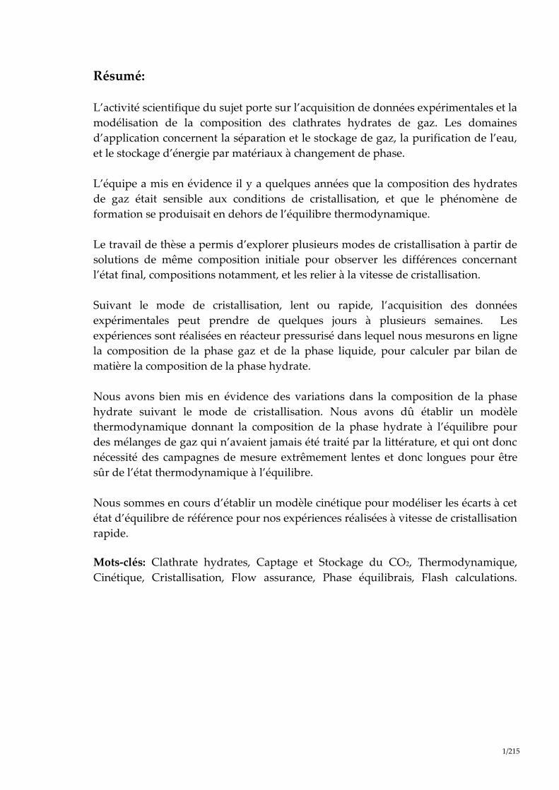
Résumé:

L’activité scientifique du sujet porte sur l’acquisition de données expérimentales et la

modélisation de la composition des clathrates hydrates de gaz. Les domaines

d’application concernent la séparation et le stockage de gaz, la purification de l’eau,

et le stockage d’énergie par matériaux à changement de phase.

L’équipe a mis en évidence il y a quelques années que la composition des hydrates

de gaz était sensible aux conditions de cristallisation, et que le phénomène de

formation se produisait en dehors de l’équilibre thermodynamique.

Le travail de thèse a permis d’explorer plusieurs modes de cristallisation à partir de

solutions de même composition initiale pour observer les différences concernant

l’état final, compositions notamment, et les relier à la vitesse de cristallisation.

Suivant le mode de cristallisation, lent ou rapide, l’acquisition des données

expérimentales peut prendre de quelques jours à plusieurs semaines. Les

expériences sont réalisées en réacteur pressurisé dans lequel nous mesurons en ligne

la composition de la phase gaz et de la phase liquide, pour calculer par bilan de

matière la composition de la phase hydrate.

Nous avons bien mis en évidence des variations dans la composition de la phase

hydrate suivant le mode de cristallisation. Nous avons dû établir un modèle

thermodynamique donnant la composition de la phase hydrate à l’équilibre pour

des mélanges de gaz qui n’avaient jamais été traité par la littérature, et qui ont donc

nécessité des campagnes de mesure extrêmement lentes et donc longues pour être

sûr de l’état thermodynamique à l’équilibre.

Nous sommes en cours d’établir un modèle cinétique pour modéliser les écarts à cet

état d’équilibre de référence pour nos expériences réalisées à vitesse de cristallisation

rapide.

Mots-clés: Clathrate hydrates, Captage et Stockage du CO2, Thermodynamique,

Cinétique, Cristallisation, Flow assurance, Phase équilibrais, Flash calculations.

3/215

Summary:

The scientific goal of this thesis is based on the acquisition of experimental data and

the modeling of the composition of clathrates gas hydrate. The domains of

application concern the gas separation and storage, water purification, and energy

storage using change phase materials (PCMs).

Our research team has recently demonstrated that the composition of gas hydrates

was sensitive to the crystallization conditions, and that the phenomenon of

formation was out of thermodynamic equilibrium.

During this thesis, we have investigated several types of crystallization, which are

based on the same initial states. The goal is to point out the differences between the

initial solution composition and the final solution composition, and to establish a

link between the final state and the crystallization rate.

Depending on the rate of crystallization (slow or fast), the acquisition time of

experimental data lasted from a few days to several weeks. The experimental tests

were performed inside a stirred batch reactor (autoclave, 2.44 or 2.36 litre) cooled

with a double jacket. Real-time measurements of the composition of the gas and the

liquid phases have been performed, in order to calculate the composition of the

hydrate phase using mass balance calculations. Depending on the crystallization

mode, we have identified several variations of the composition of the hydrate phase

and final hydrate volume.

We have established a successful thermodynamic model, which indicates the

composition of the hydrate phase and hydrate volume in thermodynamic

equilibrium state using a gas mixture which had never been used before in the

literature. So this thermodynamic model has required an extremely slow

experimental test. These tests were also long in order to be sure of the

thermodynamic equilibrium state.

We are currently establishing a kinetics model in order to model the deviations from

the reference point of equilibrium of our experimental tests which were carried out

at a high crystallization rate.

Key-words: Gas Hydrates, Thermodynamic, Kinetic, Crystallization, CO2 capture

and storage, Flow assurance, Phase equilibria, Flash calculations

5/215

LIST OF FIGURE

Figure 1: Water molecules forming cages corresponding to hydrate structures, sI, sII

and sH ............................................................................................................................. 26

Figure 2: Comparison of guest molecule sizes and cavities occupied as simple

hydrates. Modified from (Carroll, 2014) .................................................................... 28

Figure 3: Lattice parameters versus temperature for varius sI Hydrates, modified

from (Hester et al., 2007) ............................................................................................... 29

Figure 4: Lattice parameters versus temperature for varius sII Hydrates, modified

from (Hester et al., 2007) ............................................................................................... 29

Figure 5: Phase diagrams of methane clathrate hydrates (with P: pressure; T:

temperature) (Adisasmito et al., 1991; De Roo et al., 1983; Deaton and Frost,

1946; Falabella, 1975; Galloway et al., 1970; Jhaveri and Robinson, 1965;

Kobayashi et al., 1949; Makogon and Sloan, 1994; Marshall et al., 1964; McLeod

and Campbell, 1961; Roberts et al., 1940; Thakore and Holder, 1987; Verma, 1974;

Yang et al., 2001). ........................................................................................................... 34

Figure 6: CH-V Equilibrium of single CO2 at temperature below the ice point. The

simuation curve is obtained with the GasHyDyn simulator, implemented with

reference parameters from Table 25 (Dharmawardhana et al., 1980) and Table 26.

(Page. 63) and Kihara parameters given in Table 28. (Page. 75). ............................ 36

Figure 7: CH-V Equilibrium of single CH4 at temperature below the ice point. The

simulation of SI structure is obtained with the GasHyDyn simulator,

implemented with reference parameters from Table 25 (Dharmawardhana et al.,

1980) and Table 26. (Page. 63) and Kihara parameters given in Table 28. (Page.

75). .................................................................................................................................... 37

Figure 8: CH-V and CH_SI-V-Lw Equilibrium of single C2H6. The simulation of SI

Structure is obtained with the GasHyDyn simulator, implemented with



Figure 9: CH-V and CH_SII-V-Lw Equilibrium of single C3H8. The simulation of SII

Structure is obtained with the GasHyDyn simulator, implemented with

6/215



Figure 10: Schematic of the principle to referring at a hypothetical reference state in

order to write the equilibrium between the clathrate hydrate phase and the

liquid phase. ................................................................................................................... 58

Figure 11: Procedure to optimise the kihara parameters ................................................ 65

Figure 12: Deviation (in %, from Eq.20) between experimental equilibrium data of

pure CO2 hydrate Experimental data are from (Yasuda and Ohmura, 2008),

(Adisasmito et al., 1991), (Falabella, 1975), (Miller and Smythe, 1970) which

cover a range of temperature from 151.52K to 282.9K and a pressure range from

0.535kPa to 4370kPa....................................................................................................... 67

Figure 13 : versus at the minimum deviation with experimental data. a value

is taken from Table 27. Pressure and temperature equilibrium data for CO2

hydrate are taken from (Yasuda and Ohmura, 2008), (Adisasmito et al., 1991),

(Falabella, 1975), (Miller and Smythe, 1970) which cover a range of temperature

from 151.52K to 282.9K and a pressure range from 0.535kPa to 4370kPa. ............ 68


is taken from Table 27. Pressure and temperature equilibrium data for CH4

hydrate are taken from (Fray et al., 2010), (Yasuda and Ohmura, 2008),

(Adisasmito et al., 1991) which cover a range of temperature from 145.75 to

286.4K and a pressure range from 2.4kPa to 10570kPa. ........................................... 69


is taken from Table 27. Pressure and temperature equilibrium data for C2H6

hydrate are taken , from (Roberts et al., 1940), (Deaton and Frost, 1946), (Reamer

et al., 1952), (Falabella, 1975), (Yasuda and Ohmura, 2008), (Mohammadi and

Richon, 2010a, 2010b), which cover a wide range of temperature from 200.08 to

287.4K and a pressure range from 8.3kPa to 3298kPa. ............................................. 70


is taken from Table 27. Pressure and temperature equilibrium data for C3H8

hydrate are taken from (Deaton and Frost, 1946), (Yasuda and Ohmura, 2008)

and (Nixdorf and Oellrich, 1997) which cover a wide range of temperature from

245 to 278.5K and a pressure range from 41kPa to 567kPa .................................... 71

k

k

k

k

7/215


is taken from Table 27. Pressure and temperature equilibrium data for CH4-C3H8

hydrate are taken from (Verma et al., 1974) and (Verma, 1974). ............................ 72

Figure 18 : versus at the minimum deviation with experimental data. SII is

assumed. a value is taken from Table 27. Pressure and temperature equilibrium

data for Xe- C3H8 hydrate is taken from (Tohidi et al., 1993). ................................. 73

Figure 19: versus at the minimum deviation with experimental data. SI is

assumed. a value is taken from Table 27. Pressure and temperature equilibrium

data for Xe-C3H8 hydrate is taken from (Tohidi et al., 1993). .................................. 73

Figure 20: versus at the minimum deviation with experimental data. a value is

taken from Table 27. Pressure and temperature equilibrium data for CO2-C3H8

hydrate is taken from (Adisasmito and Sloan, 1992). ............................................... 74

Figure 21: Schematic of the concentration profiles in the environment of a particle in

a liquid bulk.................................................................................................................... 78

Figure 22 : Influence of the stirring rate on the rate of methane dissolution in a

stirred batch reactor (Herri et al., 1999a) .................................................................... 80

Figure 23 : Shape of the Gibbs energy function during formation of a cluster of n

entities, depending on supersaturation (Herri, 1996) .............................................. 85

Figure 24: Induction time versus supersaturation during nucleation of methane

hydrate in pure water, at 1°C (Herri et al., 1999b) .................................................... 86

Figure 25: The factor versus angle according to Eq. (45) ............................................. 89

Figure 26: Association of clusters ....................................................................................... 90

Figure 27: Molar fraction of clusters at equilibrium. The index n refers to the number

of elementary units of the cluster. S is the value of the supersaturation ............... 93

Figure 28 : Elementary steps of gas integration in the vicinity of the growing hydrate

surface (Herri and Kwaterski, 2012). .......................................................................... 96

Figure 29: Double procedure of convergence to calculate the gas hydrate growing

rate G, and the gas composition , intjx around the growing hydrate. ................... 107

Figure 30: Molar composition of the hydrate phase as a function of the intrinsic

growth rates. The liquid phase is supposed to be in equilibrium with a gas phase

composed of an equimolar CO2-N2 mixture, at a pressure of 4 MPa and

temperature of 1 °C ..................................................................................................... 111

k

k

k

k

8/215

Figure 31 : Growth rate of the hydrate phase as a function of the intrinsic growth

rate. The liquid phase is assumed to be in equilibrium with a gas phase

composed of an equimolar CO2-N2 mixture at a temperature of 1 °C and a

pressure of 4 MPa ........................................................................................................ 111

Figure 32: The system of Milli-Q®-AdvantageA10 at SPIN center laboratory .......... 113

Figure 33: Experimental set-up ......................................................................................... 116

Figure 34: Schematic of Electromagnetic version of the ROLSITM Sampler injector.

........................................................................................................................................ 117

Figure 35: Schematic of the VARIAN chromatograph (Model 3800 GC) equipped

with a TCD detector. ................................................................................................... 118

Figure 36: The system of the ionic chromatography at SPIN laboratory .................... 119

Figure 37: The procedure of the high crystallization rate ............................................. 121

Figure 38: P– T evolution during equilibria experiments at high crystallization rate.

........................................................................................................................................ 121

Figure 39: The procedure of the low crystallization rate. .............................................. 122

Figure 40: P – T evolution during equilibrium experiment at low crystallization rate.

........................................................................................................................................ 122

Figure 41: Chromatogram of a liquid sample - Analysis of Lithium .......................... 123

Figure 42: Calibration curve of the ionic chromatography ........................................... 124

Figure 43: GC principle ...................................................................................................... 124

Figure 44: Calibration curve of gas chromatograph ...................................................... 127

Figure 45: Chromatogram of a sample of CO2-N2 mixtures ......................................... 129

Figure 46: Experimental equilibrium data of CO2-N2 gas hydrate at high driving

force compared with GasHyDyn predictions .......................................................... 139

Figure 47: Experimental equilibrium data of CO2-CH4-C2H4 gas hydrate at high

driving force compare with GasHyDyn predictions .............................................. 141

Figure 48: Experimental equilibrium data of CO2-CH4-C2H4 gas hydrate at low

driving force compare with GasHyDyn predictions .............................................. 142

Figure 49: Experimental equilibrium data of CH4-C3H8 gas hydrate at high and low

driving force ................................................................................................................. 145

Figure 50: Experimental equilibrium data of CH4-C2H6-C3H8 gas hydrate at low

driving force ................................................................................................................. 147

Figure 51: Example of Flash algorithm (θ=mass flow ratio between phases) ............ 153

9/215

Figure 52: Basic hydrate flash algorithm. ........................................................................ 155

Figure 53: Thermodynamic path (Bouillot and Herri, 2016). ....................................... 156

Figure 54: Algorithm to perform hydrate flash calculation with no reorganization of

the crystal phase (framework I) (Bouillot and Herri, 2016). .................................. 159

Figure 55: Mixed hydrate growth (no reorganization) (Bouillot and Herri, 2016). ... 160

Figure 56: Algorithm to perform hydrate flash calculation with reorganization of the

hydrate phase during crystallization (framework II) (Bouillot and Herri, 2016).

........................................................................................................................................ 161

Figure 57: Hydrate growth with crystal phase reorganization (framework II*)

(Bouillot and Herri, 2016). .......................................................................................... 162

Figure 58: PT diagram of experimental and predicted results of the reference case

(CO2-CH4-C2H6) at different temperatures from the same initial state. ............... 164

Figure 59: Predicted and experimental thermodynamic paths (Pressure vs

temperature during crystallization) in the reference case (left: all frameworks at

different numbers of iterations; right: framework I, N=7). .................................... 167

Figure 60: Schematic of the calculation of the Volume of Reactor ............................... 201

Figure 61: Schematic of calibration of Gas Chromatography (GC) ............................. 203

Figure 62: Calibration curve of gas chromatograph of CO2-N2 gas mixture .............. 205

Figure 63: Calibration curve of gas chromatograph of CH3-C3H8 gas mixture .......... 206

Figure 64: Calibration curve of the gas chromatograph for CO2-CH4 ......................... 207

Figure 65: Calibration curve of the gas chromatograph for C2H6-CH4 ....................... 207

Figure 66: Algorithm of calculation on the molar composition ................................... 209

10/215

11/215

LIST OF TABLE

Table 1: Structure of gas hydrates ...................................................................................... 27

Table 2: Molar Masses of Some Hydrates at 0oC .............................................................. 30

Table 3: Densities of Some Hydrates at 0oC (Carroll, 2014) ............................................ 32

Table 4: CH_SI-V-Lw Equilibrium of CO2-CH4 from (Bouchemoua et al., 2009). The

simulation curve is obtained with the GasHyDyn simulator, implemented with


(Page 63) and Kihara parameters given in Table 28. (Page. 75). ............................. 40

Table 5: CH_SI-V-Lw Equilibrium of CO2-CH4 from (Le Quang, 2013). The




Table 6: CH_SI-V-Lw Equilibrium of CO2-CH4 from (Belandria et al., 2011). The




Table 7: CH_SI-V-Lw Equilibrium of CO2-CH4 from (Seo et al., 2000). The simulation

curve is obtained with the GasHyDyn simulator, implemented with reference

parameters from Table 25 (Dharmawardhana et al., 1980) and Table 26. (Page.

63) and Kihara parameters given in Table 28. (Page. 75). ........................................ 42

Table 8: CH_SI-V-Lw Equilibrium of CO2-CH4 from (Fan and Guo, 1999). The




Table 9: CH_SI-V-Lw Equilibrium of CO2-CH4 from (Ohgaki et al., 1996). The




Table 10: CH_SI-V-Lw Equilibrium of CO2-CH4 from (Adisasmito et al., 1991). The


12/215



Table 11: CH_SI-V-Lw Equilibrium of CO2-CH4 from (Hachikubo et al., 2002). The




Table 12: CH_SI-V-Lw Equilibrium of CO2-CH4 from (Unruh and Katz, 1949). The




Table 13 : CH_SI-V-Lw Equilibrium of CH4-C2H6 from (Adisasmito and Sloan, 1992).

The simulation curve is obtained with the GasHyDyn simulator, implemented

with reference parameters from Table 25 (Dharmawardhana et al., 1980) and

Table 26. (Page. 63) and Kihara parameters given in Table 28. (Page. 75). ........... 46

Table 14: CH-V-Lw Equilibrium of CH4-C3H8 from (Verma et al., 1974). The




Table 15: CH-V-Lw Equilibrium of CH4-C3H8 from (Deaton and Frost, 1946). The




Table 16: CH-V-Lw Equilibrium of CH4-C3H8 from (McLeod and Campbell, 1961).




Table 17: CH-V-Lw Equilibrium of CH4-C3H8 from (Thakore and Holder, 1987). The




Table 18: CH-V-Lw Equilibrium of C2H6-C3H8 from (Mooijer-Van den Heuvel, 2004).


13/215



Table 19: CH-V-Lw Equilibrium of CO2-CH4-C2H6 from (Le Quang, 2013). The




Table 20: CH-V-Lw Equilibrium of CO2-CH4-C2H6 from (Kvenvolden et al., 1984).




Table 21: CH-V-Lw Equilibrium of CH4-C2H6-C3H8 from (Le Quang, 2013). The




Table 22: CH-V-Lw Equilibrium of CH4-C2H6-C3H8 C4H10(-1) from (Le Quang, 2013).




Table 23 : CH-V-Lw Equilibrium of CH4-C2H6-C3H8 C4H10(-1) from (Le Quang, 2013).




Table 24: Correlations to calculate the , , and a .kihara parameters as a function of

the pitzer acentric factor and critical coordinates Pc , Tc and Vc ..................... 60

Table 25: Mascroscopic parameters of hydrates and Ice (Sloan, 1998; Sloan and Koh,

2007) ................................................................................................................................. 63

Table 26: Reference properties of hydrates from (Sloan, 1998; Sloan and Koh, 2007) 63

Table 27: Kihara parameters after optimisation on experimental data (Herri et al.,

2011) and compared to litterature ............................................................................... 66

Table 28: Kihara parameters, after optimisation from experimental data with the

GasHyDyn simulator, implemented with reference parameters from Table 25

(Dharmawardhana et al., 1980) and Table 26. ........................................................... 75

14/215

Table 29: Nucleation of cluster of n building units, in homogeneous condition (a), at

the surface of foreign surface or parent surface (b), at a gas/liquid interface (c).

is a factor between 0 and 1 to quantify the decrease in the critical Gibbs Energy.

is the interfacial energy between the phases, hyd=hydrate phase, liq=liq solution,

gas=gas, solid=foreign or parent phase (Kashchiev and Firoozabadi, 2002a,

2002b). .............................................................................................................................. 88

Table 30: Occupancy factor of enclathrated molecules as a function of the

composition in the liquid phase. The equations of the right-hand column are

obtained from the classical Langmuir expressions from Eq. (73) (left column)

upon replacing jx by the expression of Eq. (93) (right column). ......................... 103

Table 31: Purity of Helium gas used in our experiments ............................................. 113

Table 32 : The physical properties of Lithium nitrate (LiNO3) ..................................... 114

Table 33: Molar composition of the experiments gas mixtures (standard deviation

about 3%) ...................................................................................................................... 115

Table 34 : Operating conditions of the chromatogram .................................................. 126

Table 35: SRK parameters .................................................................................................. 130

Table 36: Constants for calculating Henry’s constant (Holder et al., 1980) ................ 133

Table 37: Molar composition of the studied gas mixtures and initial conditions of

experiments. ................................................................................................................. 137

Table 38: CH_SI-V-Lw Equilibrium of CO2-N2 at quick crystallization rate procedure

versus predicted results .............................................................................................. 138

Table 39: CH_SI-V-Lw Equilibrium of CO2-CH4-C2H6 at high crystallization rate

procedure versus predicted results. .......................................................................... 140

Table 40: CH_SI-V-Lw Equilibrium of CO2-CH4-C2H6 at low crystallization rate

procedure versus predicted results. .......................................................................... 142

Table 41: CH_SI-V-Lw Equilibrium of CH4-C3H8 at high crystallization rate

procedure. ..................................................................................................................... 143

Table 42: CH_SI-V-Lw Equilibrium of CH4-C3H8 at low crystallization rate

procedure. ..................................................................................................................... 144

Table 43: Experimental and predicted pressures for the first data obtained in each

experiments (CH4-C3H8) .............................................................................................. 146

Table 44 : CH_SI-V-Lw Equilibrium of CH4-C2H6-C3H8 at high crystallization rate (Le

Quang, 2013) ................................................................................................................. 148

15/215

Table 45: CH_SI-V-Lw Equilibrium of CH4-C2H6-C3H8 at low crystallization rate

procedure. ..................................................................................................................... 148

Table 46: Quick Kihara parameters optimization of CO2, CH4 and C2H6 on a few

experimental data (Adisasmito et al., 1991; Avlonitis, 1988; Dyadin, 1996; Y. A.

Dyadin et al., 1996; Yurii A. Dyadin et al., 1996; Englezos and Bishnoi, 1991;

Larson, 1955; Le Quang et al., n.d.; Nixdorf and Oellrich, 1997; Thakore and

Holder, 1987; Yasuda and Ohmura, 2008) (* data from (Sloan and Koh, 2007)) 163

Table 47: Experimental versus predicted results for the reference case (CO2, CH4 and

C2H6) from classic thermodynamic calculations assuming a SI structure. .......... 164


C2H6) from classic thermodynamic calculations assuming a SI structure. .......... 166

Table 49: Influence of the Kihara parameters uncertainties on the flash hydrate

results (framework I, reference case). ....................................................................... 167

Table 50: Framework I (n=5 and 20) and II* predictions compared to experimental

results at quick crystallization (gas 1-2 from CO2-CH4 mixtures and 3-4-5 from

CO2-CH4-C2H6 mixtures) and slow crystallization (reference case of the present

study) ............................................................................................................................. 169

Table 51: Constants necessary for the calculation of the compressibility factor........ 200

Table 52: Experiment data ................................................................................................. 202

Table 53: The results of the calculation ............................................................................ 202

Table 54: Experiment results ............................................................................................. 204

16/215

17/215

TABLE OF CONTENTS

1. INTRODUCTION ................................................................................................................. 21

2. GAS HYDRATES ................................................................................................................ 25

2.1. STRUCTURE OF GAS HYDRATES .................................................................... 25

2.2. PHYSICAL PROPERTIES OF GAS HYDRATES ............................................... 30

2.2.1 Molar Mass 30

2.2.2 Density 31

2.2.3 Volume of Gas in Hydrate 32

2.2.4 The Hydration Number 33

2.2.5 Phase diagrams of the hydrates 33

3. EQUILIBRIUM DATA .......................................................................................................... 35

3.1. PURE HYDRATES ................................................................................................. 36

3.1.1 CO2 Clathrate Hydrate equilibrium data 36

3.1.2 CH4 Clathrate Hydrate equilibrium data 37

3.1.3 C2H6 Clathrate Hydrate equilibrium data 38

3.1.4 C3H8 Clathrate Hydrate equilibrium data 39

3.2. MIXED HYDRATES .............................................................................................. 40

3.2.1 CO2-CH4 Clathrate Hydrate equilibrium data 40

3.2.2 CO2-C2H6 Clathrate Hydrate equilibrium data 46

3.2.3 CH4-C3H8 Clathrate Hydrate equilibrium data 47

3.2.4 C2H6-C3H8 Clathrate Hydrate equilibrium data 51

3.2.5 CO2-CH4-C2H6 Clathrate Hydrate equilibrium data 52

3.2.6 CH4-C2H6-C3H8 Clathrate Hydrate equilibrium data 53

3.2.7 CH4-C2H6-C3H8 C4H10(-1) Clathrate Hydrate equilibrium data 54

4. THERMODYNAMIC OF GAS HYDRATES ............................................................................ 57

4.1. MODELLING OF ....................................................................................... 57

4.2. MODELLING OF ..................................................................................... 61

4.3. ADJUSTMENT OF MODELS PARAMETERS ................................................... 63

4.3.1 Determination of the reference parameters 64

4.3.2 Determination of the kihara parameters 66

5. HYDRATES UNDER NON EQUILIBRIUM CONDITIONS ....................................................... 77

H

w

β

w

18/215

5.1. INTRODUCTION ................................................................................................. 77

5.2. GENERALITIES ABOUT THE CRYSTALLIZATION OF GAS

HYDRATES ............................................................................................................ 78

5.3. MODELLING THE GAS/LIQUID TRANSFER IN A BATCH

REACTOR .............................................................................................................. 79

5.4. MODELLING THE NUCLEATION ................................................................... 80

5.4.1 Primary nucleation from the model of Volmer and Weber (1926) 81

5.4.2 Primary nucleation from a rigorous kinetic approach 89

5.4.3 Primary nucleation for chemical engineers 93

5.4.4 Secondary nucleation 94

5.5. MODELLING THE GROWTH ............................................................................ 95

5.5.1 Enclathration during crystallisation 98

5.5.2 Discussion 108

5.5.3 Numerical application 109

5.6. Conclusion ............................................................................................................ 112

6. MATERIALS AND METHODS .......................................................................................... 113

6.1. CHEMICALS ....................................................................................................... 113

6.1.1 Deionized water (H2O) 113

6.1.2 Helium (He) 113

6.1.3 Lithium Nitrate (LiNO3) 114

6.1.4 Gas mixtures (CO2, N2, CH4, C2H6, C3H8) 114

6.2. EXPERIMENTAL DEVICE ................................................................................ 115

6.3. EXPERIMENTAL PROCEDURE ...................................................................... 120

6.3.1 High crystallization rate 120

6.3.2 Low crystallization rate 121

6.4. OPERATING PROTOCOLS .............................................................................. 123

6.4.1 Determination of the concentration of lithium by ionic

chromatography. 123

6.4.2 Calibrating the gas chromatograph (TCD) 124

6.4.3 Mass balance calculation 129

7. EXPERIMENTALS RESULTS AND DISCUSSIONS............................................................... 137

7.1. CO2-N2 GAS MIXTURES .................................................................................... 138

7.2. CO2-CH4-C2H6 GAS MIXTURE ......................................................................... 139

19/215

7.3. CH4-C3H8 GAS MIXTURES ................................................................................ 143

7.4. CH4-C2H4-C3H8 GAS MIXTURES ....................................................................... 147

7.5. Conclusion ............................................................................................................ 149

8. FLASH CALCULATION .................................................................................................... 151

8.1. INTRODUCTION ................................................................................................ 151

8.2. STATE OF THE ART ........................................................................................... 152

8.2.1 Usual flash calculations 152

8.2.2 Flash hydrate modeling 153

8.3. BASIC ALGORITHM .......................................................................................... 154

8.4. HYDRATE FLASH ALGORITHM WITHOUT CRYSTAL

REORGANIZATION ........................................................................................... 157

8.5. HYDRATE FLASH ALGORITHM WITH CRYSTAL

REORGANIZATION ........................................................................................... 161

8.6. KIHARA PARAMETERS OPTIMIZATION .................................................... 162

8.7. RESULTS ............................................................................................................... 163

8.7.1. Thermodynamic equilibrium 163

8.7.2. Flash results 165

8.8. KIHARA UNCERTAINTIES .............................................................................. 167

8.9. MIXED HYDRATE CRYSTALLIZATION ....................................................... 168

8.10. CONCLUSION ..................................................................................................... 170

9. CONCLUSION .................................................................................................................. 173

10. LIST OF SYMBOLS ............................................................................................................. 175

11. REFERENCES .................................................................................................................... 183

12. APPENDIX 1: CALCULATION OF THE VOLUME OF REACTOR ......................................... 199

13. APPENDIX 2: CALIBRATION OF GAS CHROMATOGRAPHY ............................................ 203

14. APPENDIX 3: EVALUATION OF ERRORS CALCULATION ................................................ 209

20/215

21/215

1. INTRODUCTION

The Gas hydrates are encountered in many systems where the pressure is high

enough and the temperature low enough to cristallize the liquid water and the gas

phase in a solid called clathrate hydrate.

Applications of gas hydrate formation are numerous and a complete reviewing has

been achieved in the framework of the French ANR national program called

SECOHYA coordinated by our team: - gas production from methane hydrate

bearing sediments and CO2 injection, - natural gas storage and transportation under

the form of pellets, - thermal storage by using slurries of semi-clathrates hydrates

from quaternary ammonium salts, - separation of gases: methane, nitrogen, carbon

dioxide, - food preservation by using ozone clahtrates. The applications currently

developed in our team are Air conditioning (Darbouret et al., 2005; Douzet et al.,

2013), CO2 capture (Duc et al., 2007; Galfré et al., 2014; Herri et al., 2014, 2011;

Herslund et al., 2013), and Methane hydrate bearing sediments for gas production

(Tonnet and Herri, 2009). We collaborate also with other teams to develop science on

Food preservation (Muromachi et al., 2013), Sequestration (Burnol et al., 2015) or

technology on Waste Wate treatment.

On other hand, gas hydrate formation is a main concern as a risk in the oil

production, especially in deep sea pipelines where they can plug the facilities by

forming both a crust on the pipelines, and also increasing the viscosity of fluids. This

subject has been a main concern for our team and still continues to be (Cameirao et

al., 2012; Fidel-Dufour et al., 2005; Herri et al., 2009; Leba et al., 2010).

Lastly, Gas Hydrates are a concern in astrophysics and planetary sciences as its

formation, even at very low pressure conditions, is still possible due to the

exceptional low temperature. For example, our team is collaborating on the possible

methane enclathratation during seasonal cycles on Mars. It could explain the

anormal preservation of methane in the Martian atmosphere (Chassefière et al., 2013;

Herri and Chassefière, 2012).

In each of the applications, the experimentations and modelling imply to develop

knowledge about thermodynamics and kinetics. In fact, the process of crystallization

of gas hydrates involves many elementary steps such as nucleation, growth,

agglomeration, attrition….. Each of the steps is depending on a driving force (i.e.

super-saturation) in between equilibrium conditions (thermodynamic) actual

conditions. Actual conditions are governed in the end by mass transfers of gases

from the gas phase to the hydrate structure. For example, in a liquid bulk solution,

the gas fraction in the liquid is dependent, on one side of the rate of gas dissolution

at the Gas/liquid interface, and dependent on the other side of the gas consumption

22/215

rate by hydrate crystallization (to be more precise, dependent at the first order of the

growth rate).

My work is a contribution to evaluate the composition of gas hydrate under a null-

driving force (experiments at pseudo equilibrium) and under high driving force. In

fact, from theoretical speculations, (Herri and Kwaterski, 2012) has justified that the

composition could not only fixed by thermodynamic, but could be also dependent

on the relative rates of mass transfers of the different gases.

It opened for my team, a new field of research, because it allows orientating the

crystallization in a favorable direction, for example in gas separation process such as

the capture of CO2, and it introduces the possibility to modify the crystallization

with the use of kinetic additives or specific geometries.

For my proper concern, the possibility to form hydrate under un-equilibrium

conditions opened a main question irelative to the flow assurance management for

oil production. In factthe volume of hydrates that are formed could be badly

evaluated from simulators working at equilibrium conditions.

This manuscript is organized as following:

The first part of the document deals with structure (Chapter 2), composition

(Chapter 3) and thermodynamic modeling (Chapter 4) of gas hydrates. It gives the

fudamentals to model equilibrium conditions.

As said before, my work has been conducted half under equilibrium conditions, and

half under non equilibrium conditions. Chapter 5 is a focus to couple kinetics and

thermodynamics and to show how much the composition of gas hydrate could be

not only dependent on thermodynamics but also on kinetics.

Following is my first personal contribution. It has been to monitor experimentally

the compositions of hydrates under equilibrium and non-equlibrium conditions

(Chapters 6 and 7) by using an original experimental proctocol developed in the our

laboratory during the Ph.D. work of A. Bouchemoua (Herri et al., 2011). On my side,

I designed two experimental procedures, under low rate or high rate of

cristallisation, and I observed the difference in the composition of the hydrates that

are formed from a same mixture. The gas mixture has been choiced to be

representative of the oil production industry, CO2, CH4, C2H6, C3H8.

My second concern has been to support the modelling approach from two points of

view:

- Firstly, I gave equilibrium data to implement our in-house simulation

software, called GasHyDyn (presented at the beginning of section §3 Page 21).

23/215

In the document, we show the difficulty in retrieving thermodynamic

paramaters from the experiments, because of the difficulty to be sure that the

data are at equilibrium, and/or because of the necessity to run complex

mixtures as some gas hydrates formers can not form pure gas hydrates.

- Secondly, I gave non-equilibrium data and supported a new approach to

model the composition of hydrates from a flash calculation (Chapter 8), and

to understand the composition of hydrates not from a kinetic modelling as

given in Chapter 5, but from a succession of quasi-equilibrium.

As a conclusion of this work, we emphasize that equilibrium of hydrate from gas

mixture needs to perform experiments at a very low rate, and so during very long

time of experiments, from weeks to months.

24/215

25/215

2. GAS HYDRATES

2.1. STRUCTURE OF GAS HYDRATES

The clathrates are ice-like compounds in the sense that they correspond to a re-

organisation of the water molecules to form a solid. The crystallographic structure is

based on H-bonds. The clathrates of water are also designated improperly as

“porous ice” because the water molecules build a solid network of cavities in which

gases, volatile liquids or other small molecules could be captured.

The clathrates of gases, called gas hydrates, have been studied intensively due to

their occurrence in deep sea pipelines where they cause serious problems of flow

assurance.

There are two structures of hydrates commonly encountered in the petroleum

business (Sloan and Koh, 2007). These are called structure I and structure II,

sometimes referred to as type I and II. A third structure of hydrate that also may be

encountered is structure H (structures I and II hydrates can form in the presence of a

single hydrate former, but structure H requires two formers to be present, a small

molecule, such as methane, and a larger type H forming molecule), but it is less

commonly encountered (Carroll, 2014). Each structure is a combination of different

types of polyhedra sharing faces between them. (Jeffrey, 1984) suggested the

nomenclature (ef) to describe the polyhedra to form the primitive cells (where (e) is

the number of edges, and (f) the number of faces). Currently, three different

structures have been established precisely, called I, II and H (Sloan, 1998; Sloan and

Koh, 2007). The three structures are formed by a total of five different water cavities

are the 512, 51262, 51264, 51268 and the 435663 (Sloan, 1998; Sloan and Koh, 2007). A

schematic of these cavities may be found in Figure 1 which shows the polyhedra

involved in structure I, II and H. On this figure, the water molecule is on the corner

of the polyhedral. The edges represent hydrogen bonds. The physical properties of

the hydrate cavities and unit cells are provided in Table 1. Structures I, II, and H will

be reviewed in more detail throughout this part. In its pure form, the unit cell of the

structure I (sI) hydrate contains two small 512 and six large 51262 cavities, in which

only methane, ethane and carbon dioxide of the natural gas components stabilize the

structure. Structure II (sII) hydrate contains sixteen small 512 cavities and eight large

51264 cavities. The large cavity in sII can contain larger molecules (up to 6.6 Å, see in

Figure 2). This means that propane and iso-butane can stabilize this large cavity.

Alternatively, small cavities can be filled with methane, which means that natural

gas with propane or iso-butane typically forms sII hydrates. Methane will form sI

hydrate by filling both the large and the small cavities, but not sII because the

molecules are too small to stabilize the large cavities in sII. Both of these unit cell

lattice structures belong to the cubic type. The structure H (sH) hydrate is contains

three 512, two 435663 and one 51268 cavities, being significantly more complex (Sum et

26/215

al., 2009). This hydrate structure forms a hexagonal unit cell. A given hydrate

structure is typically determined by the size and shape of the guest molecule. Each

cavity may encapsulate one or in rare cases more guest molecules of proper sizes. Of

course, the presence of the guest molecule is necessary to stabilize the crystalline

water structure at temperatures well above the normal freezing point.

Figure 1: Water molecules forming cages corresponding to hydrate structures, sI, sII

and sH

Based on the knowledge about the hydrate structure for a given gas composition, it

is possible to calculate the relative water/guest ratio known as the ideal hydration

number:

𝑛ℎ𝑦𝑑 =

𝑛𝑢𝑚𝑏𝑒𝑟 𝑜𝑓 𝑤𝑎𝑡𝑒𝑟 𝑚𝑜𝑙𝑒𝑐𝑢𝑙𝑒𝑠

𝑛𝑢𝑚𝑏𝑒𝑟 𝑜𝑓 𝑔𝑎𝑠 𝑚𝑜𝑙𝑒𝑐𝑢𝑙𝑒𝑠 (1)

Pure methane will occupy the 2 small and the 6 large cavities of sI. With 46 water

molecules in a unit cell, the ideal hydration number becomes 5.75. For an natural gas

mixture of methane, ethane and propane, where propane and ethane stabilize the 8

large cavities of sII, methane enter the 16 small cavities, and the unit cell has 136

water molecules, the ideal hydration number becomes 5.67 (Figure 1 and Figure 2).

512

512

62

512

64

435

66

3

512

68

6

8

1

2

3

16

2

Cavity Types Hydrate structure “Guest” Molecules

46 H2O

34 H2O

136 H2O

Structure I

Structure II

Structure H

Methane, Ethane, Carbon

dioxide, etc.

Propane, Isobutane, etc.

Methane + Neohexane,

Methane + Cycloheptane,

etc.

27/215

Table 1: Structure of gas hydrates

SI SII SH

Cavity 512 51262 512 51264 512 435663 51268

Type of cavity (j: indexing number)

1 2 1 3 1 5 4

Typical formers CH4, C2H6, H2S, CO2 N2, C3H8, i-C4H10 See belowo

Number of cavities

(mj) 2 6 16 8 3 2 1

Average cavity

radius (nm)(1) 0.395 0.433 0.391 0.473 0.391 0.406 0.571

Variation in radius,

% (2) 3.4 14.4 5.5 1.73

Coordination

number 20 24 20 28 20 20 36

Number of water

molecules 42 136 134

Cell parameters (nm) 0a = 1.1956 (3) 0a =1.7315 (4) a=1.2217, b=1.0053 (5)

Thermal expansivity

1 a

a T

(6)

2

1 2 0 3 0a a T T a T T

2 30 32

1 0 0 0

0

1 exp2 3

a a aaa T T T T T T

a

4

1

7

2

11

3

1.128010

2 1.800310

3 1.589810

a

a

a

5

1

8

2

11

3

6.765910

2 6.170610

3 6.264910

a

a

a

Cell volume (nm3) 1.709 (3) 5.192 (4) 1.22994 (5)

(1) From (Sloan, 1998, p. 33)

(2) Variation in distance of oxygen atoms from centre of cages (Sloan, 1998, p. 33).

(3) For ethane hydrate, from (Udachin et al., 2002).

(4) For tetrahydrofuran hydrate, from (Udachin et al., 2002).

(5) For methylcyclohexane-methane hydrate, from (Udachin et al., 2002).

(6) From (Hester et al., 2007).

o 2-methylbutane, 2,2-dimethylbutane, 2,3-dimethylbutane, 2,2,3-trimethylbutane, 2,2-

dimethylpentane, 3,3-dimethylpentane, methylcyclopentane, ethylcyclopentane,

methylcyclohexane, cycloheptane, and cyclooctane. Most of these components are

not commonly found in natural gas.

28/215

Figure 2: Comparison of guest molecule sizes and cavities occupied as simple

hydrates. Modified from (Carroll, 2014)

More details about the cell parameters can be found in (Hester et al., 2007). They

measured the hydrate lattice parameters for four Structure I (C2H6, CO2, 47% C2H6 +

53% CO2, and 85% CH4 + 15% CO2) and seven Structure II (C3H8, 60% CH4 + 40%

Ar

Kr N2 O2

CH4

Xe, H2S

CO2

C2H6

c-C3H8

(CH2)3O

C3H8

Iso-C4H10

n-C4H10

4Å

5Å

6Å

7Å

No hydrates ??

(hydrogen hydrates)

Structure II- large and small cavities

sII: 512 + 51264

Structure I- large and small cavities

sI: 512 + 51262

Structure I- large cavities only

sI: 51262

Structure II- large cavities only

sII: 51264

Structure H- large, medium and small cavities

sH: 512 + 435663 + 51268

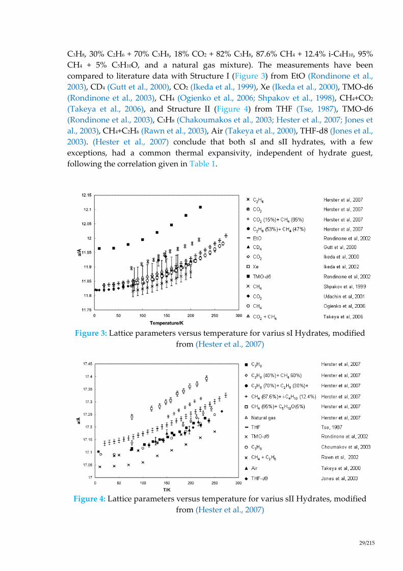
29/215

C3H8, 30% C2H6 + 70% C3H8, 18% CO2 + 82% C3H8, 87.6% CH4 + 12.4% i-C4H10, 95%

CH4 + 5% C5H10O, and a natural gas mixture). The measurements have been

compared to literature data with Structure I (Figure 3) from EtO (Rondinone et al.,

2003), CD4 (Gutt et al., 2000), CO2 (Ikeda et al., 1999), Xe (Ikeda et al., 2000), TMO-d6

(Rondinone et al., 2003), CH4 (Ogienko et al., 2006; Shpakov et al., 1998), CH4+CO2

(Takeya et al., 2006), and Structure II (Figure 4) from THF (Tse, 1987), TMO-d6

(Rondinone et al., 2003), C3H8 (Chakoumakos et al., 2003; Hester et al., 2007; Jones et

al., 2003), CH4+C2H6 (Rawn et al., 2003), Air (Takeya et al., 2000), THF-d8 (Jones et al.,

2003). (Hester et al., 2007) conclude that both sI and sII hydrates, with a few

exceptions, had a common thermal expansivity, independent of hydrate guest,

following the correlation given in Table 1.

Figure 3: Lattice parameters versus temperature for varius sI Hydrates, modified

from (Hester et al., 2007)

Figure 4: Lattice parameters versus temperature for varius sII Hydrates, modified

from (Hester et al., 2007)

30/215

2.2. PHYSICAL PROPERTIES OF GAS HYDRATES

2.2.1 MOLAR MASS

The molar mass (molecular weight) of a hydrate can be determined from its crystal

structure and the degree of saturation (An exception is CSMHYD, which does give

saturation values). Then, the newer CSMGEM gives composition of the hydrate

phase, but not specifically the cell saturation). The molar mass of the hydrate, M, is

expressed as follow (Carroll, 2014):

𝑀 =

𝑁𝑤𝑀𝑤 + ∑ ∑ 𝑌𝑖𝑗𝑣𝑖𝑀𝑗𝑛𝑖=1

𝑐𝑗=1

𝑁𝑤 + ∑ ∑ 𝑌𝑖𝑗𝑣𝑖𝑛𝑖=1

𝑐𝑗=1

(2)

where NW is the number of water molecules per unit cell (46 for Structure I, 136 for

Structure II, and 34 for Structure H, (see on Table 1)), MW is the molar mass of water,

Yij is the fractional occupancy of cavities of structure i by component j, vi is the

number of structure i cavities, 𝑛 is the number of cavities of structure i (two for both

Structure I and II, but is three for Structure H), and c is the number of components in

the cell.

Although this equation looks fairly complicated, it is just accounting for all of the

molecules present and then using a number average to get the molar mass.

Table 2: Molar Masses of Some Hydrates at 0oC

(Note: calculated using Eq. (2). The saturation values were calculated using

CSMHYD)

Saturation

Gas Hydrate

structures

Small Large Molar mass

(g/mol)

Methane I 0.8723 0.9730 17.74

Ethane I 0.0000 0.9864 19.39

Propane II 0.0000 0.9987 19.46

Iso-Butane II 0.0000 0.9987 20.24

CO2 I 0.7295 0.9813 21.59

On Table 2 summarizes the molar masses of a few hydrate formers. It is a little

surprising that the molar masses of all six components are approximately around

31/215

equal (17÷22g/mol). This is because the hydrate is composed mostly of water (18.015

g/mol).

It is interesting that the molar masses of hydrates are a function of the temperature

and the pressure, since the degree of saturation is a function of these variables. We

usually think of molar masses as being constants for a given substance.

2.2.2 DENSITY

The density of a hydrate, 𝜌, can be calculated using the following formula below

(Carroll, 2014):

𝜌 =

𝑁𝑤𝑀𝑊 + ∑ ∑ 𝑌𝑖𝑗𝑣𝑖𝑀𝑗𝑛𝑖=1

𝑐𝑗=1

𝑁𝐴𝑉𝑐𝑒𝑙𝑙 (3)

Where 𝑁𝐴 is Avogadro’s number (6.023.1023 molecules/mole), 𝑉𝑐𝑒𝑙𝑙 is the volume of

the unit cell (Table 1), NW is the number of water molecules per unit cell), MW is the

molar mass of water, Yij is the fractional occupancy of cavities of structure i by

component j, vi is the number of structure i cavities, 𝑛 is the number of cavities of

structure i (two for both Structure I and II, but is three for Structure H), and c is the

number of components in the cell.

Eq. (3) can be reduced for a single component in either a Structure I or Structure II

hydrate to:

𝜌 =

𝑁𝑤𝑀𝑤 + (𝑌1𝑣1 + 𝑌2𝑣2)𝑀𝑗

𝑁𝐴𝑉𝑐𝑒𝑙𝑙 (4)

Again, although Eq. (3) and (4) look complicated, they are just accounting for the

number of molecules in a unit cell of hydrate. The mass of all these molecules

divided by the unit volume of the crystal gives the density of the hydrate.

The densities of some pure hydrates at 0oC are given in Table 3. Note that the

densities of the hydrates of the hydrocarbons are similar to ice.

At last, for an empty hydrate structure, the formula is simple:

𝑀 =

𝑁𝑤𝑀𝑤

𝑁𝐴𝑉𝐶𝑒𝑙𝑙 (5)

32/215

Table 3: Densities of Some Hydrates at 0oC (Carroll, 2014)

Hydrate structure

(I, II, or H)

Density

(g/cm3)

Methane I 0.913

Ethane I 0.967

Propane II 0.899

Isobutane II 0.934

CO2 I 1.107

Ice - 0.917

Water - 1.000

This equation gives a density of 790 kg/m3 for structure I and 785kg/m3 for structure

II. It is a usefull equation to calculate the hydrate volume from the crystallized mass

of water.

2.2.3 VOLUME OF GAS IN HYDRATE

Some interesting properties of methane hydrate at 0°C: the density is 913 kg/m3, the

molar mass (molecular weight) is 17.74 kg/kmol, and methane concentration is 14.1

mol percent-this means there are 141 molecules of methane per 859 molecules of

water in the methane hydrate.

This information can be used to determine the volume of gas in the methane

hydrate. From the density, 1 m3 of hydrate has a mass of 913 kg. Converting this to

moles, 913/17.74 = 51.45 kmol of hydrate, of which 7.257 kmol are methane.

Ideal gas law can be used to calculate the volume of gas when expanded to standard

conditions (15 oC and 1 atm or 101.325 kPa)

𝑉 =

𝑛𝑅𝑇

𝑃=

(7.257)(8.314)(15 + 273.15)

101.325= 171.5 (𝑆𝑚3) (6)

33/215

Therefore, 1 m3 of hydrate contains about ~170 Sm3 of methane gas at standard

conditions (15 oC and 1 atm or 101.325 kPa). According to Kvenvolden (Kvenvolden,

1993) 1m3 gas hydrate may release about 164 m3 methane and 0.8 m3 of water under

standard temperature and pressure (STP) condition.

2.2.4 THE HYDRATION NUMBER

An important property is the hydration number. This value describes the

relationship between the water molecules and molecules (Thiam, 2008). The

knowledge of this property directly provides information which corresponds to a

correct structure is given by Eq. (1) (section §2.1. Page. 25).

If all the cavities were completely occupied, the hydration number corresponds to

the ratio between the number of water molecules, and the number of cavities.

However, experience shows that the cavities are partially occupied, and that we

must define an occupancy rate, to which we return more detail in the section on

Thermodynamics modelling. The actual number of hydration is given by:

𝑛ℎ𝑦𝑑 =

𝑛𝑢𝑚𝑏𝑒𝑟 𝑜𝑓 𝑤𝑎𝑡𝑒𝑟 𝑚𝑜𝑙𝑒𝑐𝑢𝑙𝑒𝑠 𝑝𝑒𝑟 𝑢𝑛𝑖𝑡 𝑐𝑒𝑙𝑙

∑ ∑ 𝑣𝑖𝜃𝑗𝑖𝑁𝑇

𝑖=1𝐶𝑇𝑗=1

(7)

Where 𝒗𝒊 is the number of cavities of the type 𝑖 per molecule of water, 𝜃𝑗𝑖 is the

occupancy rate of cavities 𝑖 by each gas 𝑗 (the occupancy rate is a function of

thermodynamic conditions (pressure and temperature) and specific physical

properties to the gas molecule, such as size, shape, or its mode of interaction with

host molecules), 𝐶𝑇 is the number of species of present gases, 𝑁𝑇 is the number of

different cavities in the elementary network. If we know the number of hydration

and the formed structure, can then determine other physical quantities such that the

molar volume or density.

2.2.5 PHASE DIAGRAMS OF THE HYDRATES

Phase diagrams define stability regions of gas hydrates and the existing phases in

the system. Usually, these phase diagrams represent the liquid-hydrate equilibrium

in pressure vs temperature. Indeed, for a given temperature, knowing the pressure is

directly linked to the knowledge of the gas solubility (thus the gas molecule

concentration in the liquid phase). Figure 5 shows the phase diagram of methane

from literature.

34/215

Figure 5: Phase diagrams of methane clathrate hydrates (with P: pressure; T:

temperature) (Adisasmito et al., 1991; De Roo et al., 1983; Deaton and Frost, 1946;

Falabella, 1975; Galloway et al., 1970; Jhaveri and Robinson, 1965; Kobayashi et al.,

1949; Makogon and Sloan, 1994; Marshall et al., 1964; McLeod and Campbell, 1961;

Roberts et al., 1940; Thakore and Holder, 1987; Verma, 1974; Yang et al., 2001).

On this figure, four different phases coexist around point M: ice, liquid water, gas,

and hydrate. The lower left side (zone I) corresponds to the ice phase. The upper left

side (zone G) corresponds to hydrate phase. Between the two zones is the ice-

hydrate equilibrium curve. The bottom right area (zone L) is the liquid aqueous

phase, and the upper right the hydrate phase again (zone H). Between zone L and H

is the liquid-hydrate equilibrium. Between zones I and L is the ice-liquid

equilibrium.

Based on the model of (Klauda and Sandler, 2005), a prediction for the distribution

of methane hydrate in ocean sediment is presented on a 1° latitude by 1° longitude

(1° × 1°) global grid. From that detailed prediction, it is estimated that the global gas

hydrates in marine sediments contain 1.2 × 1017 m3 of methane gas (expanded to

atmospheric conditions), or, equivalently, 74 400 Gt of CH4 in ocean hydrates, which

is 3 orders of magnitude larger than worldwide conventional natural gas reserves.

Of this number, (Klauda and Sandler, 2005) estimated that 4.4 × 1016 m3 of methane

expanded to Standard Temperature and Pressure (STP) exists on the continental

margins, which represents one of the largest sources of hydrocarbon on Earth.

Zone G

Zone I

Zone H

Zone L M

35/215

3. EQUILIBRIUM DATA

The NIST Standard Reference Database #156 is an open access data base which gives

the equilibrium data in multiphase systems with Clathrate Hydrates (CH), Vapor

(V), Liquid water (Lw) or Ice (I), Liquid hydrocarbon (LHC) for many pure

components or mixtures. This data base extends the data from (Sloan, 2005, 1998):

(http://gashydrates.nist.gov/).

The data base implemented in our in-house software, GasHyDyn, also offers a free

access to many equilibrium data. All the following equilibrium data are extracted

from this data base. The GasHyDyn database has been completed from the NIST

database, literature survey and our own experimental data.

Gashydyn software is developed at Saint-Etienne School of Mines by The Hydrate

team. It is based on classic Van der Waals and Plateeuw model for the prediction of

gas hydrate equilibria with the constant of Parrish and Prausnitz. This software

predicts the thermodynamics and the cage occupancy of stable hydrate structures

(sI, sII, and sH) from a given pressure or temperature and gas phase composition:

(http://www.emse.fr). This software can also be used for both pure and mixed gas

hydrates. The software allows takes in account constants ∆𝜇𝑤0

, ∆𝐶𝑝0, ∆ℎ𝑤

0 and 𝑎,

∆vw0 , ∆μw

0 , ∆Cp0, ∆hw

0 from different authors. More details can be founded in section

of the thermodynamic (presented in section §4. Page. 57).

In the next subsection will be provided pure and mixed hydrate equilibrium data.

These data are relevant to this work since the same gas molecules were used.

http://gashydrates.nist.gov/

http://www.emse.fr)/

36/215

3.1. PURE HYDRATES

3.1.1 CO2 CLATHRATE HYDRATE EQUILIBRIUM DATA

Figure 6: CH-V Equilibrium of single CO2 at temperature below the ice point. The



(Page. 63) and Kihara parameters given in Table 28. (Page. 75).

37/215

3.1.2 CH4 CLATHRATE HYDRATE EQUILIBRIUM DATA

Figure 7: CH-V Equilibrium of single CH4 at temperature below the ice point. The

simulation of SI structure is obtained with the GasHyDyn simulator, implemented

with reference parameters from Table 25 (Dharmawardhana et al., 1980) and Table

26. (Page. 63) and Kihara parameters given in Table 28. (Page. 75).

0.000001

0.00001

0.0001

0.001

0.01

0.1

1

10

0 50 100 150 200 250 300

Temperature [K]P

[M

Pa

]

Fray et al, 2010

Yasuda and Ohmura, 2008

Mohammadi and Richon, 2008

Makogon and Sloan, 1995

Falabella and Vanpee, 1974

Delsemme and Wenger, 1970

Deaton and Frost, 1946

sI-GasHyDyn simulation

38/215

3.1.3 C2H6 CLATHRATE HYDRATE EQUILIBRIUM DATA

Figure 8: CH-V and CH_SI-V-Lw Equilibrium of single C2H6. The simulation of SI

Structure is obtained with the GasHyDyn simulator, implemented with reference

parameters from Table 25 (Dharmawardhana et al., 1980) and Table 26. (Page. 63)

and Kihara parameters given in Table 28. (Page. 75).

1

10

100

1000

10000

200 220 240 260 280 300

Temperature [K]

Pre

ssu

re [

kP

a]

Avlonitis et al, 1988

Mohammadi and Richon, 2010


Deaton and Frost,1946

Holder and Grigoriou, 1980

Holder and Hand, 1982

Reamer et al., 1952

Robert et al., 1940


Falabella, 1975

Galloway et al, 1970

GasHyDyn Simulation - SI Structure

39/215

3.1.4 C3H8 CLATHRATE HYDRATE EQUILIBRIUM DATA

Figure 9: CH-V and CH_SII-V-Lw Equilibrium of single C3H8. The simulation of SII

Structure is obtained with the GasHyDyn simulator, implemented with reference



10

100

1000

240 250 260 270 280 290

Temperature [K]

Pre

ssu

re [kP

a]

Goddard, 1981

Holder and Kamath, 1982



Englezos and Ngan, 1993

Kubota and al, 1984

Verma, 1974

Nixdorf and Oellrich, 1997

Patil, S.L., 1987

Reamer et al, 1952

Robinson and Mehta, 1971

Miller and Strong, 1946

Thakore and Holder, 1987

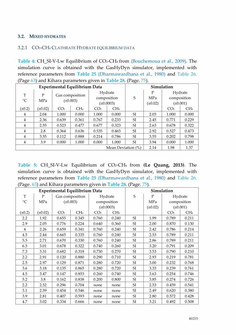
40/215

3.2. MIXED HYDRATES

3.2.1 CO2-CH4 CLATHRATE HYDRATE EQUILIBRIUM DATA

Table 4: CH_SI-V-Lw Equilibrium of CO2-CH4 from (Bouchemoua et al., 2009). The



(Page 63) and Kihara parameters given in Table 28. (Page. 75).

Experimental Equilibrium Data Simulation

T

°C

P

MPa

Gas composition

(±0.003)

Hydrate

composition

(±0.0003)

S

P

MPa

(±0.02)

Hydrate

composition

(±0.001)

(±0.2) (±0.02) CO2 CH4 CO2 CH4 CO2 CH4

4 2.04 1.000 0.000 1.000 0.000 SI 2.03 1.000 0.000

4 2.36 0.639 0.361 0.767 0.233 SI 2.45 0.771 0.229

4 2.55 0.523 0.477 0.677 0.323 SI 2.63 0.678 0.322

4 2.8 0.364 0.636 0.535 0.465 SI 2.92 0.527 0.473

4 3.55 0.112 0.888 0.214 0.786 SI 3.55 0.202 0.798

4 3.9 0.000 1.000 0.000 1.000 SI 3.94 0.000 1.000

Mean Deviation (%) 2.14 1.98 1.37

Table 5: CH_SI-V-Lw Equilibrium of CO2-CH4 from (Le Quang, 2013). The




Experimental Equilibrium Data Simulation T

°C

P

MPa

Gas composition

(±0.003)

Hydrate

composition

(±0.0003)

S P

MPa

(±0.02)

Hydrate

composition

(±0.001)

(±0.2) (±0.02) CO2 CH4 CO2 CH4 CO2 CH4

2.2 1.92 0.655 0.345 0.760 0.240 SI 1.99 0.789 0.211

2.9 2.05 0.776 0.224 0.640 0.360 SI 2.00 0.870 0.130

4 2.26 0.659 0.341 0.760 0.240 SI 2.42 0.786 0.214

4.5 2.44 0.665 0.335 0.760 0.240 SI 2.53 0.789 0.211

5.5 2.71 0.670 0.330 0.760 0.240 SI 2.86 0.789 0.211

6.5 3.01 0.678 0.322 0.740 0.260 SI 3.20 0.791 0.209

7.3 3.31 0.682 0.318 0.730 0.270 SI 3.53 0.790 0.210

2.2 2.91 0.120 0.880 0.290 0.710 SI 2.93 0.219 0.781

2.5 2.97 0.129 0.871 0.280 0.720 SI 3.00 0.232 0.768

3.6 3.18 0.135 0.865 0.280 0.720 SI 3.33 0.239 0.761

4.5 3.47 0.147 0.853 0.260 0.740 SI 3.63 0.254 0.746

5.2 3.8 0.162 0.838 0.200 0.800 SI 3.85 0.274 0.726

2.2 2.52 0.296 0.704 none none SI 2.53 0.459 0.541

3.1 2.59 0.454 0.546 none none SI 2.49 0.620 0.380

3.9 2.81 0.407 0.593 none none SI 2.80 0.572 0.428

4.7 3.02 0.334 0.666 none none SI 3.21 0.492 0.508

41/215

5.6 3.29 0.340 0.660 none none SI 3.52 0.495 0.505

6.6 3.53 0.345 0.655 none none SI 3.93 0.495 0.505

7.3 3.87 0.350 0.650 none none SI 4.25 0.497 0.503

3.4 3.33 0.127 0.873 0.311 0.689 SI 3.29 0.227 0.773

4.4 3.53 0.134 0.866 0.309 0.691 SI 3.62 0.235 0.765

4.9 3.71 0.141 0.859 0.308 0.692 SI 3.80 0.244 0.756

5.8 4.03 0.151 0.849 0.304 0.696 SI 4.14 0.256 0.744

6.8 4.45 0.163 0.837 0.295 0.705 SI 4.57 0.270 0.730

7.8 4.93 0.175 0.825 0.260 0.740 SI 5.06 0.283 0.717

2.2 2.91 0.120 0.880 0.290 0.710 SI 2.93 0.219 0.781

2.5 2.97 0.129 0.871 0.280 0.720 SI 3.00 0.232 0.768

3.6 3.18 0.135 0.865 0.280 0.720 SI 3.33 0.239 0.761

4.5 3.47 0.147 0.853 0.260 0.740 SI 3.63 0.254 0.746

5.2 3.8 0.162 0.838 0.200 0.800 SI 3.85 0.274 0.726

Mean Deviation (%) 3.8 15.7 11.5

Table 6: CH_SI-V-Lw Equilibrium of CO2-CH4 from (Belandria et al., 2011). The





T

°C

P

MPa

Gas composition

(±0.003)

Hydrate

composition

(±0.003)

S P

MPa

Hydrate

composition

(±0.001)

(±0.2) (±0.02) CO2 CH4 CO2 CH4 (±0.02) CO2 CH4

0.45 2.234 0.141 0.859 none none SI 2.41 0.255 0.745

0.45 2.416 0.125 0.875 none none SI 2.43 0.230 0.770

0.45 2.44 0.081 0.919 0.096 0.904 SI 2.55 0.156 0.844

0.45 1.844 0.345 0.655 0.549 0.451 SI 2.03 0.520 0.480

0.45 1.941 0.288 0.712 0.392 0.608 SI 2.12 0.455 0.545

0.45 2.048 0.220 0.780 0.294 0.706 SI 2.24 0.369 0.631

0.45 1.51 0.630 0.370 0.884 0.116 SI 1.67 0.775 0.225

0.45 1.607 0.545 0.455 0.801 0.199 SI 1.77 0.708 0.292

2.05 2.583 0.166 0.834 0.338 0.662 SI 2.77 0.289 0.711

2.05 2.712 0.129 0.871 none none SI 2.84 0.233 0.767

2.05 2.766 0.086 0.914 0.179 0.821 SI 2.98 0.162 0.838

2.05 2.123 0.384 0.616 0.650 0.350 SI 2.33 0.556 0.444

2.05 2.22 0.302 0.698 0.586 0.414 SI 2.48 0.466 0.534

2.05 2.4 0.228 0.772 0.366 0.634 SI 2.63 0.375 0.625

2.05 1.792 0.657 0.343 0.831 0.169 SI 1.96 0.790 0.210

2.05 1.865 0.565 0.435 0.752 0.248 SI 2.07 0.720 0.280

2.95 2.813 0.179 0.821 0.264 0.736 SI 3.00 0.306 0.694

2.95 3.025 0.134 0.866 0.239 0.761 SI 3.12 0.239 0.761

2.95 3.027 0.096 0.904 0.238 0.762 SI 3.23 0.178 0.822

2.95 2.318 0.405 0.595 0.644 0.356 SI 2.43 0.575 0.425

2.95 2.503 0.315 0.685 0.400 0.600 SI 2.70 0.478 0.522

2.95 2.69 0.232 0.768 0.312 0.688 SI 2.88 0.377 0.623

2.95 1.985 0.669 0.331 0.877 0.123 SI 2.14 0.797 0.203

42/215

2.95 2.174 0.579 0.421 0.784 0.216 SI 2.26 0.728 0.272

4.95 3.416 0.202 0.798 0.233 0.767 SI 3.64 0.331 0.669

4.95 3.631 0.139 0.861 0.225 0.775 SI 3.83 0.241 0.759

4.95 3.802 0.103 0.897 0.148 0.852 SI 3.95 0.185 0.815

4.95 3.037 0.323 0.677 0.457 0.543 SI 3.33 0.479 0.521

4.95 3.319 0.233 0.767 0.273 0.727 SI 3.55 0.372 0.628

4.95 2.45 0.694 0.306 none none SI 2.65 0.808 0.192

4.95 2.58 0.609 0.391 0.786 0.214 SI 2.77 0.745 0.255

6.05 3.565 0.202 0.798 0.266 0.734 SI 4.09 0.327 0.673

7.05 4.486 0.147 0.853 0.307 0.693 SI 4.76 0.246 0.754

7.05 4.655 0.108 0.892 0.245 0.755 SI 4.90 0.188 0.812

7.05 3.541 0.344 0.656 0.727 0.273 SI 4.14 0.492 0.508

7.05 4.109 0.235 0.765 0.339 0.661 SI 4.46 0.365 0.635

7.05 3.139 0.620 0.380 0.860 0.140 SI 3.53 0.744 0.256

7.05 3.481 0.490 0.510 0.788 0.212 SI 3.75 0.635 0.365

9.05 5.767 0.114 0.886 0.276 0.724 SI 6.08 0.191 0.809

11.05 7.19 0.115 0.885 0.107 0.893 SI 7.65 0.184 0.816


Table 7: CH_SI-V-Lw Equilibrium of CO2-CH4 from (Seo et al., 2000). The simulation

curve is obtained with the GasHyDyn simulator, implemented with reference




T

°C

P

MPa

Gas composition

(±0.003)

Hydrate

composition

(±0.003)

S P

MPa (±0.02)

Hydrate

composition

(±0.001)

(±0.2) (±0.02) CO2 CH4 CO2 CH4 CO2 CH4

-0.05 2 0.284 0.716 0.915 0.085 SI 1.92 0.453 0.547

0.95 2 0.403 0.597 0.936 0.064 SI 2.03 0.579 0.421

2.25 2 0.608 0.392 0.982 0.018 SI 2.06 0.753 0.247

3.15 2 0.794 0.206 0.997 0.003 SI 2.04 0.881 0.119

0.65 2.6 0.129 0.871 0.662 0.338 SI 2.48 0.236 0.764

1.75 2.6 0.234 0.766 0.847 0.153 SI 2.54 0.384 0.616

3.15 2.6 0.415 0.585 0.927 0.073 SI 2.56 0.583 0.417

4.35 2.6 0.641 0.359 0.981 0.019 SI 2.55 0.772 0.228

4.95 2.6 0.834 0.166 0.994 0.006 SI 2.46 0.902 0.098

3.45 3.5 0.133 0.867 0.647 0.353 SI 3.29 0.236 0.764

4.45 3.5 0.252 0.748 0.733 0.267 SI 3.32 0.397 0.603

5.85 3.5 0.419 0.581 0.890 0.110 SI 3.45 0.575 0.425

6.75 3.5 0.611 0.389 0.952 0.048 SI 3.43 0.738 0.262

7.35 3.5 0.834 0.166 0.993 0.007 SI 3.30 0.896 0.104

Mean Deviation (%) 3.3 34.8 866.5

43/215

Table 8: CH_SI-V-Lw Equilibrium of CO2-CH4 from (Fan and Guo, 1999). The





°C

P

MPa

Gas composition

(±0.003)

Hydrate

composition

(±0.003)

S P

MPa

(±0.02)

Hydrate

composition

(±0.001)

(±0.2) (±0.02) CO2 CH4 CO2 CH4 CO2 CH4

0.35 1.1 0.965 0.035 none none SI 1.37 0.982 0.018

0.45 1.16 0.965 0.035 none none SI 1.38 0.982 0.018

0.55 1.2 0.965 0.035 none none SI 1.40 0.982 0.018

4.05 1.95 0.965 0.035 none none SI 2.07 0.981 0.019

4.45 1.94 0.965 0.035 none none SI 2.17 0.981 0.019

4.75 2.05 0.965 0.035 none none SI 2.25 0.981 0.019

7.25 3 0.965 0.035 none none SI 3.07 0.979 0.021

8.55 3.73 0.965 0.035 none none SI 3.65 0.978 0.022

9.15 4.8 0.965 0.035 none none SI 3.98 0.977 0.023

Mean Deviation (%) 12.2 none none

Table 9: CH_SI-V-Lw Equilibrium of CO2-CH4 from (Ohgaki et al., 1996). The





°C

P

MPa

Gas composition

(±0.003)

Hydrate

composition

(±0.003)

S P

MPa

(±0.02)

Hydrate

composition

(±0.001)

(±0.2) (±0.02) CO2 CH4 CO2 CH4 CO2 CH4

7.15 3.04 1.000 0.000 1.000 0.000 SI 2.98 1.000 0.000

7.15 3.24 0.683 0.317 0.840 0.160 SI 3.46 0.792 0.208

7.15 3.38 0.585 0.415 0.800 0.200 SI 3.55 0.717 0.283

7.15 3.6 0.488 0.512 0.670 0.330 SI 3.85 0.632 0.368

7.15 3.64 0.450 0.550 0.690 0.310 SI 3.93 0.598 0.402

7.15 3.67 0.448 0.552 0.680 0.320 SI 3.93 0.596 0.404

7.15 3.71 0.429 0.571 0.610 0.390 SI 3.98 0.578 0.422

7.15 3.77 0.384 0.616 0.600 0.400 SI 4.09 0.533 0.467

7.15 3.86 0.357 0.643 0.590 0.410 SI 4.16 0.505 0.495

7.15 4.22 0.241 0.759 0.440 0.560 SI 4.49 0.372 0.628

7.15 4.31 0.215 0.785 0.390 0.610 SI 4.57 0.339 0.661

7.15 4.32 0.217 0.783 0.360 0.640 SI 4.57 0.342 0.658

7.15 4.34 0.203 0.797 0.370 0.630 SI 4.61 0.323 0.677

7.15 4.37 0.203 0.797 0.350 0.650 SI 4.61 0.323 0.677

7.15 4.37 0.183 0.817 0.360 0.640 SI 4.68 0.297 0.703

7.15 4.44 0.179 0.821 0.360 0.640 SI 4.70 0.291 0.709

7.15 4.5 0.169 0.831 0.350 0.650 SI 4.73 0.277 0.723

7.15 4.57 0.144 0.856 0.320 0.680 SI 4.82 0.242 0.758

44/215

7.15 3.98 0.302 0.698 0.530 0.470 SI 4.31 0.445 0.555

7.15 4 0.310 0.690 0.520 0.480 SI 4.29 0.454 0.546

7.15 4.01 0.311 0.689 0.550 0.450 SI 4.28 0.455 0.545

7.15 4.06 0.288 0.712 0.510 0.490 SI 4.35 0.429 0.571

7.15 4.07 0.293 0.707 0.520 0.480 SI 4.33 0.434 0.566

7.15 4.15 0.268 0.732 0.470 0.530 SI 4.41 0.405 0.595

7.15 4.2 0.245 0.755 0.450 0.550 SI 4.48 0.377 0.623

7.15 4.58 0.141 0.859 0.320 0.680 SI 4.83 0.237 0.763

7.15 4.63 0.143 0.857 0.290 0.710 SI 4.83 0.240 0.760

7.15 4.75 0.104 0.896 0.240 0.760 SI 4.96 0.181 0.819

7.15 4.85 0.090 0.910 0.230 0.770 SI 5.03 0.159 0.841

7.15 4.99 0.065 0.935 0.160 0.840 SI 5.14 0.118 0.882

7.15 5.46 0.000 1.000 0.000 1.000 SI 5.44 0.000 1.000


Table 10: CH_SI-V-Lw Equilibrium of CO2-CH4 from (Adisasmito et al., 1991). The





°C

P

MPa

Gas composition

(±0.003)

Hydrate

composition

(±0.003)

S P

MPa

(±0.02)

Hydrate

composition

(±0.001)

(±0.2) (±0.02) CO2 CH4 CO2 CH4 CO2 CH4

0.55 2.52 0.100 0.900 none none SI 2.53 0.189 0.811

2.65 3.1 0.090 0.910 none none SI 3.15 0.168 0.832

4.65 3.83 0.080 0.920 none none SI 3.90 0.148 0.852

7.05 4.91 0.080 0.920 none none SI 5.02 0.143 0.857

10.05 6.8 0.080 0.920 none none SI 6.98 0.135 0.865

11.95 8.4 0.080 0.920 none none SI 8.71 0.130 0.870

14.05 10.76 0.090 0.910 none none SI 11.20 0.136 0.864

1.45 2.59 0.140 0.860 none none SI 2.67 0.252 0.748

3.75 3.24 0.130 0.870 none none SI 3.40 0.231 0.769

5.95 4.18 0.130 0.870 none none SI 4.28 0.225 0.775

8.45 5.38 0.130 0.870 none none SI 5.57 0.217 0.783

10.85 7.17 0.130 0.870 none none SI 7.40 0.207 0.793

12.95 9.24 0.120 0.880 none none SI 9.60 0.183 0.817

14.25 10.95 0.130 0.870 none none SI 11.30 0.189 0.811

0.65 2.12 0.250 0.750 none none SI 2.24 0.408 0.592

6.25 3.96 0.220 0.780 none none SI 4.13 0.350 0.650

10.25 6.23 0.220 0.780 none none SI 6.51 0.329 0.671

12.05 7.75 0.210 0.790 none none SI 8.16 0.304 0.696

14.45 10.44 0.250 0.750 none none SI 11.10 0.327 0.673

0.55 1.81 0.440 0.560 none none SI 1.92 0.616 0.384

3.75 2.63 0.420 0.580 none none SI 2.73 0.585 0.415

7.55 4.03 0.400 0.600 none none SI 4.24 0.547 0.453

9.95 5.43 0.390 0.610 none none SI 5.70 0.519 0.481

11.95 6.94 0.390 0.610 none none SI 7.42 0.499 0.501

45/215

14.25 9.78 0.390 0.610 none none SI 10.41 0.465 0.535

2.45 1.99 0.500 0.500 none none SI 2.25 0.664 0.336

5.35 2.98 0.470 0.530 none none SI 3.15 0.626 0.374

7.75 4.14 0.400 0.600 none none SI 4.34 0.545 0.455

8.65 4.47 0.410 0.590 none none SI 4.76 0.550 0.450

11.95 6.84 0.440 0.560 none none SI 7.29 0.546 0.454

14.25 9.59 0.450 0.550 none none SI 10.23 0.517 0.483

1.45 1.66 0.730 0.270 none none SI 1.75 0.842 0.158

3.25 2.08 0.700 0.300 none none SI 2.13 0.818 0.182

5.05 2.58 0.680 0.320 none none SI 2.70 0.798 0.202

7.05 3.28 0.680 0.320 none none SI 3.43 0.790 0.210

8.85 4.12 0.670 0.330 none none SI 4.33 0.772 0.228

0.55 1.45 0.790 0.210 none none SI 1.54 0.883 0.117

2.75 1.88 0.780 0.220 none none SI 1.97 0.873 0.127

4.65 2.37 0.760 0.240 none none SI 2.47 0.855 0.145

6.45 2.97 0.750 0.250 none none SI 3.07 0.843 0.157

8.45 3.79 0.740 0.260 none none SI 3.97 0.827 0.173

9.55 4.37 0.850 0.150 none none SI 4.41 0.898 0.102


Table 11: CH_SI-V-Lw Equilibrium of CO2-CH4 from (Hachikubo et al., 2002). The





°C

P

MPa

Gas composition

(±0.003)

Hydrate

composition

(±0.003)

S P

MPa

(±0.02)

Hydrate

composition

(±0.001)

(±0.2) (±0.02) CO2 CH4 CO2 CH4 CO2 CH4

0.78 1.349 1.000 0.000 1.000 0.000 SI 1.41 1.000 0.000

3.65 1.806 1.000 0.000 1.000 0.000 SI 1.94 1.000 0.000

4.9 2.204 1.000 0.000 1.000 0.000 SI 2.25 1.000 0.000

-9.98 0.774 1.000 0.000 1.000 0.000 SI 0.79 1.000 0.000

-5.04 0.921 1.000 0.000 1.000 0.000 SI 0.96 1.000 0.000

-1.92 1.029 1.000 0.000 1.000 0.000 SI 1.09 1.000 0.000

4.13 2.187 1.000 0.000 1.000 0.000 SI 2.06 1.000 0.000

-4.75 2.324 0.000 1.000 0.000 1.000 SI 2.23 0.000 1.000

-1.87 2.527 0.000 1.000 0.000 1.000 SI 2.45 0.000 1.000

-1.9 1.271 0.770 0.230 none none SI 1.25 0.873 0.127

-1.74 1.434 0.500 0.500 none none SI 1.52 0.676 0.324

-1.78 2.022 0.250 0.750 none none SI 1.87 0.413 0.587


46/215

Table 12: CH_SI-V-Lw Equilibrium of CO2-CH4 from (Unruh and Katz, 1949). The





°C

P

MPa

Gas composition

(±0.003)

Hydrate

composition

(±0.003)

S P

MPa

(±0.02)

Hydrate

composition

(±0.001)

(±0.2) (±0.02) CO2 CH4 CO2 CH4 CO2 CH4

5.75 3.46 0.300 0.700 none none SI 3.69 0.449 0.551

5.75 3.43 0.360 0.640 none none SI 3.45 0.516 0.484

7.75 4.24 0.320 0.680 none none SI 4.56 0.461 0.539

9.75 5.17 0.280 0.720 none none SI 5.91 0.404 0.596

11.55 6.47 0.230 0.770 none none SI 7.50 0.332 0.668

2.35 1.99 0.600 0.400 none none SI 2.09 0.747 0.253

6.05 3.08 0.440 0.560 none none SI 3.48 0.594 0.406

3.25 3.2 0.125 0.875 none none SI 3.25 0.224 0.776

5.25 3.95 0.085 0.915 none none SI 4.13 0.155 0.845

7.85 5.1 0.070 0.930 none none SI 5.52 0.125 0.875

10.65 6.89 0.055 0.945 none none SI 7.61 0.094 0.906

6.45 3 0.710 0.290 none none SI 3.13 0.814 0.186

9.05 4.27 0.610 0.390 none none SI 4.57 0.723 0.277

10.65 5.27 0.520 0.480 none none SI 5.88 0.633 0.367

12.35 6.89 0.410 0.590 none none SI 7.70 0.514 0.486

12.55 7 0.410 0.590 none none SI 8.00 0.510 0.490

Mean Deviation (%) 8.2 none None

3.2.2 CO2-C2H6 CLATHRATE HYDRATE EQUILIBRIUM DATA

Table 13 : CH_SI-V-Lw Equilibrium of CH4-C2H6 from (Adisasmito and Sloan, 1992).

The simulation curve is obtained with the GasHyDyn simulator, implemented with




°C

P

MPa

Gas composition

(±0.003)

Hydrate

composition

(±0.003)

S P

MPa

(±0.02)

Hydrate

composition

(±0.001)

(±0.2) (±0.02) CO2 C2H6 CO2 C2H6 CO2 CO2 H6

0.55 0.57 0.220 0.780 none none SI 0.49 0.192 0.808

2.45 0.70 0.202 0.798 none none SI 0.60 0.189 0.811

4.35 0.87 0.189 0.811 none none SI 0.75 0.189 0.811

6.15 1.09 0.193 0.807 none none SI 0.92 0.198 0.802

7.95 1.41 0.246 0.754 none none SI 1.13 0.230 0.770

9.75 1.75 0.256 0.744 none none SI 1.39 0.241 0.759

11.95 2.39 0.317 0.683 none none SI 1.83 0.275 0.725

3.35 0.85 0.428 0.572 none none SI 0.73 0.299 0.701

47/215

5.25 1.08 0.417 0.583 none none SI 0.89 0.300 0.700

7.05 1.35 0.406 0.594 none none SI 1.08 0.300 0.700

8.85 1.72 0.400 0.600 none none SI 1.32 0.303 0.697

10.65 2.19 0.402 0.598 none none SI 1.63 0.309 0.691

12.65 2.83 0.389 0.611 none none SI 2.05 0.309 0.691

14.65 3.83 0.398 0.602 none none SI 2.64 0.321 0.679

0.55 0.57 0.220 0.780 none none SI 0.49 0.192 0.808


3.2.3 CH4-C3H8 CLATHRATE HYDRATE EQUILIBRIUM DATA

Table 14: CH-V-Lw Equilibrium of CH4-C3H8 from (Verma et al., 1974). The





°C

P

MPa

Gas composition

(±0.003)

Hydrate

composition

(±0.003)

S P

MPa

(±0.02)

Hydrate

composition

(±0.001)

(±0.2) (±0.02) CH4 C3H8 CH4 C3H8 CH4 C3H8

1.75 0.263 0.2375 0.7625 none none SI 0.34 0.119 0.881

3.25 0.35 0.2375 0.7625 none none SI 0.40 0.127 0.873

4.65 0.443 0.2375 0.7625 none none SI 0.48 0.135 0.865

5.95 0.56 0.2375 0.7625 none none SI 0.56 0.142 0.858

7.05 0.689 0.2375 0.7625 none none SI 0.65 0.149 0.851

8.25 0.83 0.2375 0.7625 none none SI 0.75 0.156 0.844

1.25 0.27 0.371 0.629 none none SI 0.35 0.159 0.841

2.75 0.343 0.371 0.629 none none SI 0.42 0.167 0.833

3.95 0.419 0.371 0.629 none none SI 0.49 0.174 0.826

5.45 0.536 0.371 0.629 none none SI 0.58 0.182 0.818

7.05 0.691 0.371 0.629 none none SI 0.71 0.191 0.809

9.15 0.945 0.371 0.629 none none SI 0.92 0.202 0.798


1.75 0.26 0.238 0.763 none none SII 0.19 0.324 0.676

3.25 0.35 0.238 0.763 none none SII 0.25 0.353 0.647

4.65 0.44 0.238 0.763 none none SII 0.30 0.379 0.621

5.95 0.56 0.238 0.763 none none SII 0.37 0.403 0.597

7.05 0.69 0.238 0.763 none none SII 0.44 0.422 0.578

8.25 0.83 0.238 0.763 none none SII 0.52 0.441 0.559

1.25 0.27 0.371 0.629 none none SII 0.17 0.382 0.618

2.75 0.34 0.371 0.629 none none SII 0.22 0.408 0.592

3.95 0.42 0.371 0.629 none none SII 0.26 0.427 0.573

5.45 0.54 0.371 0.629 none none SII 0.32 0.450 0.550

7.05 0.69 0.371 0.629 none none SII 0.40 0.472 0.528

9.15 0.95 0.371 0.629 none none SII 0.52 0.498 0.502


48/215

Table 15: CH-V-Lw Equilibrium of CH4-C3H8 from (Deaton and Frost, 1946). The





°C

P

MPa

Gas composition

(±0.003)

Hydrate

composition

(±0.003)

S P

MPa

(±0.02)

Hydrate

composition

(±0.001)

(±0.2) (±0.02) CH4 C3H8 CH4 C3H8 CH4 C3H8

1.65 0.27 0.362 0.638 none none SI 0.37 0.159 0.841

4.45 0.44 0.362 0.638 none none SI 0.51 0.174 0.826

7.25 0.69 0.362 0.638 none none SI 0.72 0.189 0.811

1.65 0.37 0.712 0.288 none none SI 0.61 0.274 0.726

4.45 0.54 0.712 0.288 none none SI 0.85 0.288 0.712

7.25 0.80 0.712 0.288 none none SI 1.18 0.302 0.698

10.05 1.15 0.712 0.288 none none SI 1.67 0.318 0.682

1.65 0.55 0.883 0.117 none none SI 1.08 0.412 0.588

4.45 0.78 0.883 0.117 none none SI 1.49 0.431 0.569

7.25 1.11 0.883 0.117 none none SI 2.10 0.453 0.547

10.05 1.56 0.883 0.117 none none SI 2.99 0.481 0.519

1.65 0.81 0.952 0.048 none none SI 1.73 0.592 0.408

4.45 1.14 0.952 0.048 none none SI 2.38 0.618 0.382

7.25 1.59 0.952 0.048 none none SI 3.31 0.649 0.351

10.05 2.23 0.952 0.048 none none SI 4.66 0.685 0.315

1.65 1.15 0.974 0.026 none none SI 2.17 0.720 0.280

4.45 1.59 0.974 0.026 none none SI 2.96 0.745 0.255

7.25 2.19 0.974 0.026 none none SI 4.08 0.773 0.227

10.05 3.01 0.974 0.026 none none SI 5.67 0.804 0.196

1.65 1.63 0.990 0.010 none none SI 2.67 0.868 0.132

4.45 2.25 0.990 0.010 none none SI 3.59 0.883 0.117

4.45 2.26 0.990 0.010 none none SI 3.59 0.883 0.117

7.25 3.12 0.990 0.010 none none SI 4.87 0.900 0.100

9.95 4.36 0.990 0.010 none none SI 6.61 0.917 0.083


1.65 0.27 0.362 0.638 none none SII 0.18 0.385 0.615

4.45 0.44 0.362 0.638 none none SII 0.28 0.432 0.568

7.25 0.69 0.362 0.638 none none SII 0.41 0.472 0.528

1.65 0.37 0.712 0.288 none none SII 0.21 0.504 0.496

4.45 0.54 0.712 0.288 none none SII 0.30 0.531 0.469

7.25 0.80 0.712 0.288 none none SII 0.42 0.554 0.446

10.05 1.15 0.712 0.288 none none SII 0.59 0.573 0.427

1.65 0.55 0.883 0.117 none none SII 0.29 0.561 0.439

4.45 0.78 0.883 0.117 none none SII 0.40 0.578 0.422

7.25 1.11 0.883 0.117 none none SII 0.55 0.593 0.407

10.05 1.56 0.883 0.117 none none SII 0.76 0.606 0.394

1.65 0.81 0.952 0.048 none none SII 0.30 0.574 0.426

4.45 1.14 0.952 0.048 none none SII 0.56 0.608 0.392

7.25 1.59 0.952 0.048 none none SII 0.76 0.618 0.382

49/215

10.05 2.23 0.952 0.048 none none SII 1.04 0.627 0.373

1.65 1.15 0.974 0.026 none none SII 0.51 0.614 0.386

4.45 1.59 0.974 0.026 none none SII 0.70 0.624 0.376

7.25 2.19 0.974 0.026 none none SII 0.91 0.631 0.369

10.05 3.01 0.974 0.026 none none SII 1.31 0.640 0.360

1.65 1.63 0.990 0.010 none none SII 0.74 0.641 0.359

4.45 2.25 0.990 0.010 none none SII 1.01 0.649 0.351

4.45 2.26 0.990 0.010 none none SII 1.01 0.649 0.351

7.25 3.12 0.990 0.010 none none SII 1.38 0.657 0.343

9.95 4.36 0.990 0.010 none none SII 1.87 0.664 0.336


Table 16: CH-V-Lw Equilibrium of CH4-C3H8 from (McLeod and Campbell, 1961).





°C

P

MPa

Gas composition

(±0.003)

Hydrate

composition

(±0.003)

S P

MPa

(±0.02)

Hydrate

composition

(±0.001)

(±0.2) (±0.02) CH4 C3H8 CH4 C3H8 CH4 C3H8

17.35 6.93 0.965 0.035 none none SI 14.89 0.868 0.132

30.55 62.47 0.965 0.035 none none SI 86.02 0.899 0.101

31.25 68.98 0.965 0.035 none none SI 92.61 0.895 0.105

25.95 34.51 0.965 0.035 none none SI 50.26 0.913 0.087

23.45 20.86 0.965 0.035 none none SI 36.27 0.912 0.088

28.45 48.37 0.965 0.035 none none SI 68.09 0.908 0.092

30.55 62.29 0.965 0.035 none none SI 86.02 0.899 0.101

21.35 13.89 0.965 0.035 none none SI 27.05 0.905 0.095

20.15 10.45 0.965 0.035 none none SI 22.70 0.897 0.103

17.55 6.93 0.965 0.035 none none SI 15.35 0.871 0.129

19.95 7.41 0.945 0.055 none none SI 20.47 0.846 0.154

19.65 7.41 0.945 0.055 none none SI 19.61 0.843 0.157

27.45 34.58 0.945 0.055 none none SI 57.76 0.871 0.129

29.55 48.37 0.945 0.055 none none SI 73.46 0.863 0.137

31.75 62.23 0.945 0.055 none none SI 92.51 0.848 0.152

25.35 23.62 0.945 0.055 none none SI 44.48 0.874 0.126

23.05 13.89 0.945 0.055 none none SI 32.63 0.870 0.130

17.35 6.93 0.965 0.035 none none SI 14.89 0.868 0.132

Mean Deviation (%) 85 none none

17.35 6.93 0.965 0.035 none none SII 2.68 0.651 0.349

30.55 62.47 0.965 0.035 none none SII 19.73 0.690 0.310

31.25 68.98 0.965 0.035 none none SII 22.49 0.693 0.307

25.95 34.51 0.965 0.035 none none SII 8.33 0.671 0.329

23.45 20.86 0.965 0.035 none none SII 5.75 0.664 0.336

28.45 48.37 0.965 0.035 none none SII 12.99 0.680 0.320

30.55 62.29 0.965 0.035 none none SII 19.73 0.690 0.310

21.35 13.89 0.965 0.035 none none SII 4.26 0.659 0.341

50/215

20.15 10.45 0.965 0.035 none none SII 3.65 0.657 0.343

17.55 6.93 0.965 0.035 none none SII 2.75 0.652 0.348

19.95 7.41 0.945 0.055 none none SII 3.05 0.649 0.351

19.65 7.41 0.945 0.055 none none SII 2.94 0.648 0.352

27.45 34.58 0.945 0.055 none none SII 8.36 0.665 0.335

29.55 48.37 0.945 0.055 none none SII 12.11 0.671 0.329

31.75 62.23 0.945 0.055 none none SII 18.75 0.679 0.321

25.35 23.62 0.945 0.055 none none SII 6.08 0.660 0.340

23.05 13.89 0.945 0.055 none none SII 4.47 0.655 0.345

17.35 6.93 0.965 0.035 none none SII 2.68 0.651 0.349

Mean Deviation (%) 68 none none

Table 17: CH-V-Lw Equilibrium of CH4-C3H8 from (Thakore and Holder, 1987). The





°C

P

MPa

Gas composition

(±0.003)

Hydrate

composition

(±0.003)

S P

MPa

(±0.02)

Hydrate

composition

(±0.001)

(±0.2) (±0.02) CH4 C3H8 CH4 C3H8 CH4 C3H8

2 0.42 0.765 0.235 none none SI 0.73 0.304 0.696

2 0.39 0.727 0.273 none none SI 0.66 0.283 0.717

2 0.37 0.700 0.300 none none SI 0.62 0.271 0.729

2 0.30 0.516 0.484 none none SI 0.45 0.206 0.794

2 0.28 0.420 0.580 none none SI 0.30 0.161 0.839

2 0.28 0.366 0.634 none none SI 0.38 0.162 0.838

2 0.27 0.352 0.648 none none SI 0.38 0.158 0.842

2 0.25 0.190 0.810 none none SI 0.34 0.102 0.898

2 0.25 0.083 0.917 none none SI 0.32 0.053 0.947

2 0.25 0.081 0.919 none none SI 0.32 0.052 0.948

2 0.25 0.054 0.946 none none SI 0.31 0.037 0.963

2 0.25 0.046 0.954 none none SI 0.31 0.032 0.968

2 0.25 0.037 0.963 none none SI 0.31 0.026 0.974

2 0.25 0.021 0.979 none none SI 0.31 0.015 0.985

2 0.26 0.000 1.000 none none SI 0.31 0.000 1.000

5 1.31 0.956 0.044 none none SI 2.63 0.643 0.357

5 1.14 0.947 0.053 none none SI 2.43 0.602 0.398

5 0.85 0.894 0.106 none none SI 1.67 0.453 0.547

5 0.63 0.768 0.232 none none SI 1.04 0.321 0.679

5 0.50 0.530 0.470 none none SI 0.66 0.225 0.775

5 0.49 0.510 0.490 none none SI 0.64 0.219 0.781

5 0.48 0.502 0.498 none none SI 0.63 0.217 0.783

5 0.48 0.468 0.532 none none SI 0.61 0.207 0.793

5 0.48 0.412 0.588 none none SI 0.58 0.191 0.809

5 0.46 0.394 0.606 none none SI 0.57 0.186 0.814

5 0.46 0.390 0.610 none none SI 0.56 0.185 0.815

5 0.48 0.030 0.970 none none SI 0.46 0.028 0.972

51/215

5 0.48 0.026 0.974 none none SI 0.46 0.024 0.976

5 0.51 0.000 1.000 none none SI 0.46 0.000 1.000


2 0.67 0.903 0.097 none none SII 0.32 0.571 0.429

2 0.42 0.765 0.235 none none SII 0.23 0.523 0.477

2 0.39 0.727 0.273 none none SII 0.22 0.512 0.488

2 0.37 0.700 0.300 none none SII 0.22 0.504 0.496

2 0.30 0.516 0.484 none none SII 0.20 0.448 0.552

2 0.28 0.420 0.580 none none SII 0.19 0.415 0.585

2 0.28 0.366 0.634 none none SII 0.19 0.393 0.607

2 0.27 0.352 0.648 none none SII 0.19 0.387 0.613

2 0.25 0.190 0.810 none none SII 0.21 0.297 0.703

2 0.25 0.083 0.917 none none SII 0.23 0.188 0.812

2 0.25 0.081 0.919 none none SII 0.23 0.184 0.816

2 0.25 0.054 0.946 none none SII 0.24 0.141 0.859

2 0.25 0.046 0.954 none none SII 0.25 0.126 0.874

2 0.25 0.037 0.963 none none SII 0.25 0.107 0.893

2 0.25 0.021 0.979 none none SII 0.26 0.067 0.933

2 0.26 0.000 1.000 none none SII 0.28 0.000 1.000

5 1.31 0.956 0.044 none none SII 0.61 0.612 0.388

5 1.14 0.947 0.053 none none SII 0.57 0.607 0.393

5 0.85 0.894 0.106 none none SII 0.43 0.583 0.417

5 0.63 0.768 0.232 none none SII 0.34 0.550 0.450

5 0.50 0.530 0.470 none none SII 0.29 0.491 0.509

5 0.49 0.510 0.490 none none SII 0.29 0.484 0.516

5 0.48 0.502 0.498 none none SII 0.29 0.483 0.517

5 0.48 0.468 0.532 none none SII 0.29 0.474 0.526

5 0.48 0.412 0.588 none none SII 0.30 0.457 0.543

5 0.46 0.394 0.606 none none SII 0.30 0.451 0.549

5 0.46 0.390 0.610 none none SII 0.30 0.450 0.550

5 0.48 0.030 0.970 none none SII 0.47 0.138 0.862

5 0.48 0.026 0.974 none none SII 0.48 0.125 0.875


3.2.4 C2H6-C3H8 CLATHRATE HYDRATE EQUILIBRIUM DATA

Table 18: CH-V-Lw Equilibrium of C2H6-C3H8 from (Mooijer-Van den Heuvel, 2004).





°C

P

MPa

Gas composition

(±0.003)

Hydrate

composition

(±0.003)

S P

MPa

(±0.02)

Hydrate

composition

(±0.001)

(±0.2) (±0.02) CH4 C3H8 CH4 C3H8 CH4 C3H8

3.88 0.54 0.299 0.701 none none SI 0.47 0.190 0.810

4.28 0.58 0.299 0.701 none none SI 0.49 0.191 0.809

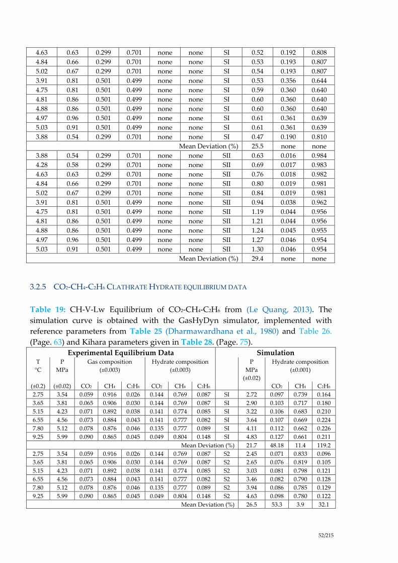
52/215

4.63 0.63 0.299 0.701 none none SI 0.52 0.192 0.808

4.84 0.66 0.299 0.701 none none SI 0.53 0.193 0.807

5.02 0.67 0.299 0.701 none none SI 0.54 0.193 0.807

3.91 0.81 0.501 0.499 none none SI 0.53 0.356 0.644

4.75 0.81 0.501 0.499 none none SI 0.59 0.360 0.640

4.81 0.86 0.501 0.499 none none SI 0.60 0.360 0.640

4.88 0.86 0.501 0.499 none none SI 0.60 0.360 0.640

4.97 0.96 0.501 0.499 none none SI 0.61 0.361 0.639

5.03 0.91 0.501 0.499 none none SI 0.61 0.361 0.639

3.88 0.54 0.299 0.701 none none SI 0.47 0.190 0.810


3.88 0.54 0.299 0.701 none none SII 0.63 0.016 0.984

4.28 0.58 0.299 0.701 none none SII 0.69 0.017 0.983

4.63 0.63 0.299 0.701 none none SII 0.76 0.018 0.982

4.84 0.66 0.299 0.701 none none SII 0.80 0.019 0.981

5.02 0.67 0.299 0.701 none none SII 0.84 0.019 0.981

3.91 0.81 0.501 0.499 none none SII 0.94 0.038 0.962

4.75 0.81 0.501 0.499 none none SII 1.19 0.044 0.956

4.81 0.86 0.501 0.499 none none SII 1.21 0.044 0.956

4.88 0.86 0.501 0.499 none none SII 1.24 0.045 0.955

4.97 0.96 0.501 0.499 none none SII 1.27 0.046 0.954

5.03 0.91 0.501 0.499 none none SII 1.30 0.046 0.954


3.2.5 CO2-CH4-C2H6 CLATHRATE HYDRATE EQUILIBRIUM DATA

Table 19: CH-V-Lw Equilibrium of CO2-CH4-C2H6 from (Le Quang, 2013). The





°C

P

MPa

Gas composition

(±0.003)

Hydrate composition

(±0.003)

P

MPa

(±0.02)

Hydrate composition

(±0.001)

(±0.2) (±0.02) CO2 CH4 C2H6 CO2 CH4 C2H6 CO2 CH4 C2H6

2.75 3.54 0.059 0.916 0.026 0.144 0.769 0.087 SI 2.72 0.097 0.739 0.164

3.65 3.81 0.065 0.906 0.030 0.144 0.769 0.087 SI 2.90 0.103 0.717 0.180

5.15 4.23 0.071 0.892 0.038 0.141 0.774 0.085 SI 3.22 0.106 0.683 0.210

6.55 4.56 0.073 0.884 0.043 0.141 0.777 0.082 SI 3.64 0.107 0.669 0.224

7.80 5.12 0.078 0.876 0.046 0.135 0.777 0.089 SI 4.11 0.112 0.662 0.226

9.25 5.99 0.090 0.865 0.045 0.049 0.804 0.148 SI 4.83 0.127 0.661 0.211

Mean Deviation (%) 21.7 48.18 11.4 119.2

2.75 3.54 0.059 0.916 0.026 0.144 0.769 0.087 S2 2.45 0.071 0.833 0.096

3.65 3.81 0.065 0.906 0.030 0.144 0.769 0.087 S2 2.65 0.076 0.819 0.105

5.15 4.23 0.071 0.892 0.038 0.141 0.774 0.085 S2 3.03 0.081 0.798 0.121

6.55 4.56 0.073 0.884 0.043 0.141 0.777 0.082 S2 3.46 0.082 0.790 0.128

7.80 5.12 0.078 0.876 0.046 0.135 0.777 0.089 S2 3.94 0.086 0.785 0.129

9.25 5.99 0.090 0.865 0.045 0.049 0.804 0.148 S2 4.63 0.098 0.780 0.122

Mean Deviation (%) 26.5 53.3 3.9 32.1

53/215

Table 20: CH-V-Lw Equilibrium of CO2-CH4-C2H6 from (Kvenvolden et al., 1984).





°C P

MPa Gas composition

(±0.003) Hydrate

composition

(±0.003)

P

MPa

(±0.02)

Hydrate

composition

(±0.001) (±0.2) (±0.02) CO2 CH4 C2H6 CO2 CH4 C2H6 CO2 CH4 C2H6

-4 3.79 0.002 0.997 0.001 none none none SI 2.25 0.004 0.984 0.011

-4 3.62 0.002 0.991 0.007 none none none SI 2.14 0.005 0.932 0.063

-4 3.50 0.003 0.995 0.003 none none none SI 2.22 0.006 0.970 0.024

-4 3.22 0.002 0.995 0.002 none none none SI 2.23 0.005 0.973 0.023

-4 2.78 0.003 0.994 0.003 none none none SI 2.22 0.007 0.970 0.024

-4 2.04 0.003 0.995 0.003 none none none SI 2.23 0.005 0.971 0.024

-4 1.20 0.005 0.992 0.003 none none none SI 2.21 0.010 0.962 0.027

Mean Deviation (%) 37.4 none none none

-4 3.79 0.002 0.997 0.001 none none none SII 1.79 0.003 0.990 0.007







Mean Deviation (%) 37.4 none none none

3.2.6 CH4-C2H6-C3H8 CLATHRATE HYDRATE EQUILIBRIUM DATA

Table 21: CH-V-Lw Equilibrium of CH4-C2H6-C3H8 from (Le Quang, 2013). The





°C P

MPa Gas composition

(±0.003) Hydrate

composition

(±0.003)

P

MPa

(±0.02)

Hydrate

composition

(±0.001) (±0.2) (±0.02) CH4 C2H6 C3H8 CH4 C2H6 C3H8 CH4 C2H6 C3H8

2.45 3.13 0.980 0.003 0.017 0.870 0.070 0.060 SI 2.58 0.784 0.018 0.198

3.15 3.36 0.979 0.004 0.017 0.855 0.079 0.067 SI 2.78 0.786 0.023 0.191

4.15 3.55 0.978 0.005 0.017 0.840 0.087 0.073 SI 3.07 0.788 0.028 0.184

4.95 3.67 0.976 0.007 0.018 0.833 0.089 0.078 SI 3.31 0.784 0.039 0.177

6.30 3.78 0.973 0.009 0.018 0.832 0.088 0.080 SI 3.75 0.778 0.050 0.172

7.70 3.94 0.968 0.012 0.020 0.828 0.087 0.085 SI 4.27 0.769 0.064 0.167

9.10 4.21 0.962 0.018 0.021 0.813 0.083 0.104 SI 4.81 0.755 0.086 0.159

54/215

10.10 4.34 0.958 0.020 0.022 0.808 0.081 0.111 SI 5.33 0.750 0.092 0.158

11.15 4.50 0.953 0.023 0.024 0.804 0.071 0.124 SI 5.88 0.742 0.101 0.157

Mean Deviation (%) 15.0 7.3 44.2 113.8

2.45 3.13 0.980 0.003 0.017 0.870 0.070 0.060 SII 0.66 0.628 0.000 0.372

3.15 3.36 0.979 0.004 0.017 0.855 0.079 0.067 SII 0.71 0.630 0.001 0.369

4.15 3.55 0.978 0.005 0.017 0.840 0.087 0.073 SII 0.80 0.633 0.001 0.366

4.95 3.67 0.976 0.007 0.018 0.833 0.089 0.078 SII 0.86 0.635 0.001 0.364

6.30 3.78 0.973 0.009 0.018 0.832 0.088 0.080 SII 0.99 0.638 0.001 0.361

7.70 3.94 0.968 0.012 0.020 0.828 0.087 0.085 SII 1.13 0.640 0.002 0.358

9.10 4.21 0.962 0.018 0.021 0.813 0.083 0.104 SII 1.30 0.642 0.003 0.355

10.10 4.34 0.958 0.020 0.022 0.808 0.081 0.111 SII 1.42 0.643 0.003 0.354

11.15 4.50 0.953 0.023 0.024 0.804 0.071 0.124 SII 1.55 0.644 0.003 0.353

Mean Deviation (%) 73.3 23.3 97.9 338.9

3.2.7 CH4-C2H6-C3H8 C4H10(-1) CLATHRATE HYDRATE EQUILIBRIUM DATA

Table 22: CH-V-Lw Equilibrium of CH4-C2H6-C3H8 C4H10(-1) from (Le Quang, 2013).





°C

P

MPa Gas composition

(±0.003)

Hydrate composition

(±0.003)

P

MPa

(±0.02)

Hydrate composition

(±0.001)

(±0.2) (±0.02) CH4 C2H6 C3H8 C3H8

-1

CH4 C2H6 C3H8 C3H8

-1 CH4 C2H6 C3H8 C3H8

-1

2.40 2.28 0.971 0.017 0.004 0.008 0.721 0.111 0.118 0.051 SI 2.80 0.833 0.117 0.050 0.000

3.45 2.31 0.967 0.019 0.005 0.008 0.723 0.109 0.118 0.050 SI 3.04 0.818 0.125 0.057 0.000

7.60 2.75 0.942 0.035 0.008 0.015 0.696 0.104 0.149 0.051 SI 4.21 0.748 0.182 0.069 0.000

9.15 2.97 0.930 0.041 0.012 0.017 0.677 0.103 0.169 0.052 SI 4.76 0.723 0.193 0.084 0.000

9.90 3.05 0.923 0.044 0.015 0.018 0.679 0.099 0.171 0.051 SI 4.99 0.704 0.194 0.101 0.000

10.80 3.12 0.915 0.046 0.020 0.019 0.686 0.097 0.167 0.050 SI 5.34 0.688 0.191 0.122 0.000

11.70 3.22 0.906 0.048 0.026 0.021 0.692 0.096 0.163 0.049 SI 5.70 0.670 0.186 0.144 0.000

12.65 3.34 0.896 0.050 0.032 0.022 0.703 0.093 0.155 0.048 SI 6.13 0.654 0.182 0.164 0.000

13.65 3.46 0.888 0.052 0.037 0.023 0.711 0.091 0.150 0.048 SI 6.79 0.650 0.178 0.173 0.000

Mean Deviation (%) 62.1 7.3 73.6 34.8 100

2.40 2.28 0.971 0.017 0.004 0.008 0.721 0.111 0.118 0.051 SII 1.11 0.671 0.010 0.304 0.014

3.45 2.31 0.967 0.019 0.005 0.008 0.723 0.109 0.118 0.050 SII 1.17 0.667 0.009 0.310 0.013

7.60 2.75 0.942 0.035 0.008 0.015 0.696 0.104 0.149 0.051 SII 1.55 0.660 0.012 0.314 0.014

9.15 2.97 0.930 0.041 0.012 0.017 0.677 0.103 0.169 0.052 SII 1.65 0.655 0.010 0.323 0.012

9.90 3.05 0.923 0.044 0.015 0.018 0.679 0.099 0.171 0.051 SII 1.64 0.650 0.009 0.331 0.010

10.80 3.12 0.915 0.046 0.020 0.019 0.686 0.097 0.167 0.050 SII 1.62 0.646 0.008 0.338 0.009

11.70 3.22 0.906 0.048 0.026 0.021 0.692 0.096 0.163 0.049 SII 1.66 0.643 0.006 0.344 0.007

12.65 3.34 0.896 0.050 0.032 0.022 0.703 0.093 0.155 0.048 SII 1.70 0.641 0.005 0.348 0.006

13.65 3.46 0.888 0.052 0.037 0.023 0.711 0.091 0.150 0.048 SII 1.81 0.640 0.005 0.349 0.006

Mean Deviation (%) 47.6 6.47 91.7 120.7 79.8

55/215

Table 23 : CH-V-Lw Equilibrium of CH4-C2H6-C3H8 C4H10(-1) from (Le Quang, 2013).





°C

P

MPa Gas composition

(±0.003)

Hydrate composition

(±0.003)

P

MPa

(±0.02)

Hydrate composition

(±0.001)

(±0.2) (±0.02) CH4 C2H6 C3H8 C3H8

-1

CH4 C2H6 C3H8 C3H8

-1 CH4 C2H6 C3H8 C3H8

-1

2.75 2.14 0.954 0.024 0.007 0.014 0.718 0.082 0.159 0.041 SI 2.68 0.769 0.151 0.080 0.000

4.30 2.16 0.955 0.024 0.007 0.014 0.717 0.082 0.160 0.041 SI 3.16 0.780 0.146 0.074 0.000

4.85 2.18 0.952 0.025 0.009 0.014 0.718 0.082 0.159 0.041 SI 3.28 0.768 0.144 0.088 0.000

5.90 2.21 0.951 0.025 0.010 0.014 0.716 0.082 0.160 0.042 SI 3.64 0.767 0.141 0.091 0.000

6.80 2.26 0.948 0.027 0.011 0.014 0.715 0.082 0.162 0.042 SI 3.92 0.757 0.143 0.100 0.000

7.45 2.36 0.939 0.030 0.015 0.016 0.713 0.079 0.166 0.042 SI 3.95 0.726 0.154 0.121 0.000

9.20 2.53 0.926 0.035 0.022 0.017 0.709 0.077 0.172 0.042 SI 4.53 0.692 0.156 0.151 0.000

11.05 2.82 0.905 0.042 0.032 0.021 0.704 0.070 0.186 0.040 SI 5.12 0.651 0.164 0.185 0.000

18.15 3.72 0.845 0.050 0.078 0.027 0.926 0.043 0.020 0.011 SI 12.34 0.668 0.128 0.203 0.000

Mean Deviation (%) 79.9 8.4 101.3 130.6 100

2.75 2.14 0.954 0.024 0.007 0.014 0.718 0.082 0.159 0.041 SII 0.95 0.651 0.008 0.324 0.016

4.30 2.16 0.955 0.024 0.007 0.014 0.717 0.082 0.160 0.041 SII 1.13 0.656 0.009 0.319 0.016

4.85 2.18 0.952 0.025 0.009 0.014 0.718 0.082 0.159 0.041 SII 1.12 0.652 0.008 0.328 0.013

5.90 2.21 0.951 0.025 0.010 0.014 0.716 0.082 0.160 0.042 SII 1.21 0.652 0.007 0.329 0.012

6.80 2.26 0.948 0.027 0.011 0.014 0.715 0.082 0.162 0.042 SII 1.27 0.650 0.007 0.333 0.011

7.45 2.36 0.939 0.030 0.015 0.016 0.713 0.079 0.166 0.042 SII 1.24 0.645 0.006 0.340 0.009

9.20 2.53 0.926 0.035 0.022 0.017 0.709 0.077 0.172 0.042 SII 1.32 0.640 0.005 0.347 0.007

11.05 2.82 0.905 0.042 0.032 0.021 0.704 0.070 0.186 0.040 SII 1.41 0.637 0.005 0.353 0.006

18.15 3.72 0.845 0.050 0.078 0.027 0.926 0.043 0.020 0.011 SII 2.33 0.638 0.003 0.356 0.003

Mean Deviation (%) 47.1 11.7 91.7 275.6 72.6

56/215

57/215

4. THERMODYNAMIC OF GAS HYDRATES

The (van der Waals and Platteeuw, 1959) describes the hydrate phase by means of

statistical thermodynamics based on the following assumptions:

- Each cavity contains at most one guest (gas) molecule

- The interaction between guest and water molecules can be described by a

pair potential function of the pair gas-molecule, and the cavity can be treated

as perfectly spherical

- The free energy contribution of the water molecules is independent of the

modes of occupancy of guest molecules. This assumption means that the gas

molecules do not deform cavities

- There is no interaction between the guests molecules in different cavities, gas

molecules interact only with the nearest water molecules.

From the previous hypotheses, statistical thermodynamics allows for the description

of the different parameters of the system and link them to quantities like

temperature, volume and chemical potential.

In the case of hydrates, in thermodynamic equilibrium, the equality of chemical

potentials of water in the liquid phase and in the hydrate phase can be written. This

relationship can be rewritten by introducing reference states. For both liquid and

hydrate phases, the reference state used in the van der Waals and Platteeuw model is

a hypothetical phase β which corresponds to the empty hydrate:

L

w

H

w

β (8)

Where H

w and L

w are the differences of the chemical potentials between

water in hydrate and liquid phase and water in the β statephase, H

w is

determined from statistical thermodynamics whereas L

w is determined by means

of relations from classical thermodynamics (Gibbs-Duhem equation).

4.1. MODELLING OF

The hydrate term is expressed as follow:

j

i

j

i

i

β RT 1lnH

w (9)

In Eq. (9) νi is the number of cavities of type i per mole of water (Table 1) and i

j is

the occupancy factor ( ]1,0[i

j ) of the cavities of type i by the gas molecule j. This

H

w

β

58/215

last parameter is very important to define the thermodynamic equilibrium and to

determine the hydrate properties.

Figure 10: Schematic of the principle to referring at a hypothetical reference state in order to write the

equilibrium between the clathrate hydrate phase and the liquid phase.

The occupancy factor is described by a model based on ideas considering the

analogy between the gas adsorption in the 3-dimensional hydrate structure and the

2-dimensional Langmuir adsorption:

- The guest molecule is adsorbed at the surface

- The adsorption energy is independent from the presence of other adsorbed

molecules

- The maximum amount of adsorbed gas corresponds to one molecule per site

(one molecule par cavity)

The expression of the occupancy factor i

j is given by:

,

,

( , )

1 ( , )

f j i ji

j

f j i j

j

C f T P

C f T P

(10)

Eq.(9) can be rewritten as:

H

w ,ln 1 ( , )β

i f j i j

i j

RT C f T P

(11)

Where ,f j iC is the Langmuir constant of component j in the cavity i. It describes the

interaction potential between the encaged guest molecule and the surrounding water

molecules evaluated by assuming a spherically symmetrical cage that can be

described by a spherical symmetrical potential:

59/215

2

0

4 ( )expi

j

w rC r dr

kT kT

(12)

Where ( )w r is the interaction potential between the cavity and the gas molecule

according to the distance r between the guest molecule and the water molecules

over the structure. The interaction potential can be determined by different models

such as e.g. the (van der Waals and Platteeuw, 1959), the (Parrish and Prausnitz,

1972) or the so-called Kihara model. The latter, being the most precise (McKoy and

Sinanoğlu, 1963), ( )w r can be expressed as follow:

54

5

61110

11

12

2)(

R

a

rRR

a

rRzrw (13)

NN

N

R

a

R

r

R

a

R

r

N11

1 (14)

The gas parameters , and a are the so-called Kihara parameters and can be

calculated from experimental data by fitting the model equations to corresponding

hydrate equilibrium experimental data. ε accounts for the maximum attractive

potential, σ to the distance from the cavity center, and a to the hard-core radius. The

first to terms are fitted from PT data (if possible), while the hard-core radius a is

usually taken from the literature (geometrical term). In this description, the

interaction potential becomes only dependent on the properties of gases (via the

Kihara parameters), and dependent of geometrical properties of the cavities (via their

coordination number z and radius R,Table 1).

Comment on the geometric description of the cavity

Theoretically, in Eq. (12), the interaction potential ( )w r needs to be integrated from 0

to infinity. It means that the gas molecule interacts with the overall structure, not

only with its first hydration shell (i.e. the water molecules of the cavity inside which

the gas molecule is encapsulated), but also interacts with other molecules localized

away from it. In fact, (John and Holder, 1982a, 1982b) have showed that 2nd and 3rd

hydration shells contribute significantly to the Langmuir constant with a resulting

change of this Langmuir constant by 1-2 orders of magnitudes (Sparks and Tester,

1992). Also, even with a rigorous integration of the interaction potential over all the

hydration shells, the (John and Holder, 1982a, 1982b) can give rigorous results only

for spherical molecules (such has Kr, Ar, CH4…). (John et al., 1985) have introduced

a correction factor to take into account the asymmetry of the encapsulated molecules.

All these refinement methods tend to give a physical signification to the interaction

potential and Kihara parameters but results in a time consuming calculation. ( )w r

60/215

For this reason, we have retained an integration of the cell potential over the first

hydration shell.

Another comment concerns the size of the cavities. (Hester et al., 2007) did an

experimental investigation of lattice parameters for sI and sII structure and different

gases (Figure 3 and Figure 4). From one gas to another one, it is showed the lattice

parameter can differ from 1%. It has been demonstrated previously via statistical

mechanics that a minor change in the lattice parameter (0.5%) can lead to a major

change in the predicted hydrate formation (e.g. > 15% at >100MPa for methane). So,

from a theoretical point of view, the size of the cavities needs to be adapted to the

component. But, this adaptation can be shifted to the kihara parameter by modifying

artificially the parameter. So, in modelling, a unique cell dimension can be

retained for all gases, and the adjustment of the model will be obtained by fitting the

kihara parameters once again.

Kihara parameters for pure substances can be evaluated from measurement of the

viscosity, calculated from second viriel coefficient, or from both (Tee et al., 1966a), or

evaluated from Henry constants (Uno et al., 1975). The Table 24 gives the

correlations to evaluate the kihara parameters, assuming a (6,12) Lennard-Jones

potential (Tee et al., 1966b), and interaction between pair of molecules.

These Kihara parameters can not be used directly to model the gas hydrate

equilibrium. In fact, in the gas hydrate modellingl, the kihara potential is assumed to

be the one from (McKoy and Sinanoğlu, 1963) in Eq. (13) and (14). Also, and more

important, and in respect to the previous comment: the interaction potential Eq. (12)

is a pseudo pair potential between a molecule on one hand, and pseudo other

molecule on the other hand consisting on the overall structure.

So, the so-called Kihara parameters need to be re-optimised on experimental data,

following a procedure given in Chapter 4 in §4.3. Page. 63.

Table 24: Correlations to calculate the , , and a .kihara parameters as a function

of the pitzer acentric factor and critical coordinates Pc , Tc and Vc

a

aa

2

2*

31

Tc

Pc 31Vc

kTc

(Tee et

al.,

1966a)

based on

viscosity 0.1501 + 2.3724 2.2802+0.2487 0.9736-0.4317

based on second

virial coefficient 0.1527 + 1.9809 2.2639+0.2487 1.0042+3.0454

based on second

virial coefficient

and viscosity

0.1495 + 1.8428 2.2631-0.3278 1.0070+2.2450

0.1495+1.8428 0.7864-0.0527 1.0030+2.2329

(Uno et

al., 1975)

based on gas

solubility 0.240 + 2.20 0.676+0.0788 1.03+1.61

61/215

From Eq. (10), we can write the average occupancy of component in the overall

structure j where i is the stoichiometry of the cavities given in:

,

,

( , )

1 ( , )

f j i j

j i i

i i f j i j

j

C f T P

C f T P

(15)

If we consider the case of a binary gas mixture of two components (j=1, 2) of

respective gas composition ,1x x

,

,

( , )

1 ( , )

f j i j

j i i

i i f j i j

j

C f T P

C f T P

(16)

4.2. MODELLING OF

The chemical potential of water in the aqueous phase is calculated by means of the

Gibbs-Duhem equation of classical thermodynamics which expresses the variation of

the chemical potential with temperature and pressure. The reference conditions are

the temperature T0 = 273.15 K and the pressure P0 = 1 bar. The difference of the

chemical potential of water between the reference phase (liquid in our case, but it

could be ice or vapour phase) and the (hypothetical) empty hydrate phase β,

w ,

can be written as follows:

PT

P

PT

T

T

PPTaRTdPvdT

T

hT

TT

,

L

w

L

w2

L

w

0

,

L

wL

w ln00

000

(17)

- The activity of water in the liquid phase, L

wa , is the product of the mole fraction

of water, wx , and its activity coefficient, L

w , hence L

ww

L

w xa . In a good

approximation, the aqueous phase can be regarded as ideal and the activity

coefficient can therefore be set to 1, resulting in w

L

w xa . However, in the

presence of polar molecules, or even salts, the system usually shows strong

deviations from ideality. In that case, L

w needs an appropriate description, as

provided e.g. by an activity coefficient model. In the specific case of salts, a

simple Pitzer-Debye-Hückel model (Ananthaswamy and Atkinson, 1984;

Pitzer, 1977) accounting for the long term electrostatic interactions only, or a

w

62/215

more elaborate model like the eNRTL (Chen et al., 1982; Chen and Evans, 1986)

or the Pitzer model (Pitzer, 1980, 1973) can be used to describe the long (and

short) range electrostatic forces. Nevertheless, in the present work, there is no

need for introducing this kind of modelsto describe L

w since the liquid phases

encountered in these experiments can be treated as pure liquid water. From a

practical point of view, L

wa is a second order parameter compared to the three

following: T

v L

w,

0

L

wP

h and 00 ,

L

wPT

.

- The value of T

v L

w is a first order parameter. It has been measured with high

accuracy by (Stackelberg and Müller, 1951) from X ray diffraction. Since that

data are believed to be very reliable, the parameter T

v L

w was taken from this

source.

- The value of 0

L

wP

h is a first order parameter as well. A refinement of the

model is given by (Sloan, 1998; Sloan and Koh, 2007) that takes into account the

temperature dependence of 0

L

wP

h using the well-known classical

thermodynamic relationship

T

TP

pPTP

dTchh0

0000

L

w,,

L

w

L

w

(18)

assuming a linear dependence of 0

L

w,P

pc on temperature according to:

0L

w,,

L

w,

L

w, 000TTbcc p

PTp

Pp (19)

The model becomes first order dependent on 00 ,

L

wPT

h (hereafter referred as

0,L

w

h ) and second order dependent on 00 ,

L

w,PT

pc (hereafter abbreviated as

0,L

w,

pc ) and L

w,pb .

- The last first order parameter of the equation is 00 ,

L

wPT

(hereafter referred

to as 0,L

w

)

63/215

Table 25: Mascroscopic parameters of hydrates and Ice (Sloan, 1998; Sloan and Koh, 2007)

Structure I Structure II 0,L

w

0,I

w

h 0,L

w

0,I

w

h

J/mol J/mol J/mol J/mol

699 0 820 0 (van der Waals and Platteeuw, 1959)

1255.2 753 795 837 (Child, 1964)

1297 1389 937 1025 (Dharmawardhana et al., 1980) ........ model 1(*)

1120 931 1714 1400 (John et al., 1985)................................. model 2(*)

1287 931 1068 764 (Handa and Tse, 1986) ....................... model 3(*)

60110,I

w

0,L

w hh , where 6011 is the enthalpy of fusion of Ice (J/mol)

(*) model refers to the model in which the 0,L

w

and 0,L

w

h reference parameters are

implemented as described in the next part of the work.

Table 26: Reference properties of hydrates from (Sloan, 1998; Sloan and Koh, 2007)

Unit Structure I Structure II

0,L

w

h J mol SI,,

I

w 00 PTh -6011

SII,,

I

w 00 PTh -6011

0

L

wT

v 10-6 m3/mol 4.5959 4.99644

0,L

w,

pc J/(mol K-1) -38.12 -38.12 L

w,pb J/(mol K-2) 0.141 0.141

4.3. ADJUSTMENT OF MODELS PARAMETERS

The phase equilibrium between the water in the hydrate and the water in the liquid

phase is described by Eq.(8).

The calculation implies to choice a set of set of Kihara parameters j , j , and ja for

each of components j, and to select the correct set of reference parameters.

Then, at a given temperature (resp. a given Pressure), and assuming a value of the

pressure (resp. the temperature), it allows the calculation of the interaction potential

in Eq.(14), then the constants of Langmuir Eq.(12), and finally in Eq.(11). Also,

it provides from Eq.(17). The calculated equilibrium pressure calcP (resp. the

calculated equilibrium temperature calcT ) corresponds to the value at which β H

w = L

w.

A special attention (first step) has to be paid when assigning value for 0 0

L

w,T P

and 0 0

L

w,T P

h since the corresponding data found in the literature vary strongly

H

w

β

w

64/215

from one author to the other, mainly due to the difficulties arising when determining

these quantities experimentally. The values can be found in the open literature as

cited by (Sloan, 1998; Sloan and Koh, 2007) and some of them are reported in Table

25. The other quantities 0,L

w

h , T

v L

w, 0,L

w,

pc , and L

w,pb are taken from Table 26.

The second step is to choose the Kihara parameters in order to fit with equilibrium

data. The number of Kihara parameters is 3: , , and .

(Mehta and Sloan, 1996) propose to fix the kihara a value first, for example by using

the correlation established by (Tee et al., 1966a, 1966b). As said previously, a is a

geometric parameter, and the volume of the molecule is supposed to be spherical. It

can be assumed it is a conservative value in the different models describing

interaction potentials.

Then, for a given set of Kihara parameters j and j , it is possible to evaluate the

deviation between the model and a set of experimental data.:

min1),(

1 exp

N

l

calc

jjP

PF (resp. min1),(

1 exp

N

l

calc

jjT

TF ) (20)

In Eq.(20), the index l assigns the specific data point and the summation has to be

performed over all N data of the set. It presents a simplified version of the deviation

function, based on deviation between the (Pressure, Temperature) coordinates at

equilibrium. Eq.(20) can be enriched to additional data such as deviation to

composition is the data are available (much harder to obtain with accuracy).

In the end, the Kihara parameters remain adjustable parameters. As it has been

claimed by (John et al., 1985) and reported by (Mehta and Sloan, 1996): the wrong

kihara parameters, wrong cell potential, wrong Langmuir constants (and we can add

from (Herri et al., 2011), the wrong reference parameters) could still lead to “right”

dissociation pressures.

4.3.1 DETERMINATION OF THE REFERENCE PARAMETERS

As we mentioned before, the values for 0 0

L

w,T P

and 0 0

L

w,T P

h strongly differ

from one author to another (Table 26). A previous work consisted in determining the

best values to use. It implied to test them against experimental results in a

thermodynamic model.

1) Choice of a set of macroscopic parameters as literature input from Table 25 and

Table 26.

2) Under the assumption of a SI and SII structure, respectively, retrieve the best

Kihara parameters by adjusting and (a value are taken from (Sloan, 2005, 1998),

by using the correlation established by (Tee et al., 1966a, 1966b), given in Table 24).

j j ja

65/215

These best values of parameters minimize the mean standard deviation between the

experimental data and the corresponding data calculated from the model (see

§4.3.2).

Figure 11: Procedure to optimise the kihara parameters

(Herri et al., 2011) determined the sensibility of the kihara parameters to the values

for 0 0

L

w,T P

and 0 0

L

w,T P

h . Table 27 shows the best kihara parameters to predict

complex H-Lw-V equilibrium, not only on pure CO2, N2 and CH4 gas, but also on

CO2-N2 , CH4-N2 and CO2-CH4 gas mixtures, giving not only the (Pressure,

Temperature, Gas mixture composition) at equilibrium but also the Hydrate

composition at equilibrium. It can be observed that the kihara parameters are

dependent on values of 0 0

L

w,T P

and 0 0

L

w,T P

h . Also, (Herri et al., 2011) showed

that a better simulation is performed as the model is implemented with parameters

from (Handa and Tse, 1986).

66/215

Table 27: Kihara parameters after optimisation on experimental data (Herri et al.,

2011) and compared to litterature

Kihara parameters regressed from experimental results from (Herri et al., 2011) and

implemented in model 1,2,3 with macroscopic parameters from Table 25. -(1) (Dharmawardhana et al., 1980) - (2) (John et al., 1985) – (3) (Handa and Tse, 1986)

CO2 CH4 N2

k

a

k

a

k

a

Model 1 170.00 2.9855 0.6805 157.85 3.1439 0.3834 126.98 3.0882 0.3526

Model 2 164.56 2.9824 0.6805 154.47 3.1110 0.3834 166.38 3.0978 0.3526

Model 3 171.41 2.9830 0.6805 158.71 3.1503 0.3834 138.22 3.0993 0.3526

Kihara parameters from literature

(Sloan, 1998;

Sloan and

Koh, 2007)

168.77 2.9818 0.6805 154.54 3.1650 0.3834 125.15 3.0124 0.3526

175.405 2.97638 0.6805 155.593 3.14393 0.3834 127.426 3.13512 0.3526

4.3.2 DETERMINATION OF THE KIHARA PARAMETERS

The reference parameters 0 0

L

w,T P

and 0 0

L

w,T P

h are taken from (Handa and Tse,

1986) in Table 25. The other reference parameters 0,L

w

h , 0

L

wT

v , 0,L

w,

pc and L

w,pb

are taken from (Sloan, 1998; Sloan and Koh, 2007) (Table 26). L

w

can be calculated

(Eq. 17) provided the water activity can be calculated. can be calculated (§4.1)

provided the kihara parameters are known. As it has been mentioned in the

previous section (§4.3.1), the determination of the kihara parameters implies to

optimise them so that the condition of equilibrium is achieved (Eq.8) following the

procedure summarized on Figure 11. It also implies to minimize the deviation

between experimental results from a data bank and simulated results.

• CO2 Kihara parameters

In the work of (Herri and Chassefière, 2012), the Kihara parameters have been

retrieved for pure CO2 clathrate hydrate by assuming a SI structure. It corresponds

to the values of Kihara parameters which minimise the deviation given in Eq.(20). It

is an optimal situation because the equilibrium data are numerous. The study

compares 32 experimental results from (Yasuda and Ohmura, 2008), (Adisasmito et

al., 1991), (Falabella, 1975), (Miller and Smythe, 1970) which cover a range of

temperature from 151.52K to 282.9K and a pressure range from 0.535kPa to 4370kPa.

H

w

β

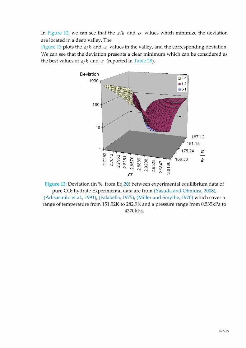
67/215

In Figure 12, we can see that the k and values which minimize the deviation

are located in a deep valley. The

Figure 13 plots the k and values in the valley, and the corresponding deviation.

We can see that the deviation presents a clear minimum which can be considered as

the best values of k and (reported in Table 28).

Figure 12: Deviation (in %, from Eq.20) between experimental equilibrium data of

pure CO2 hydrate Experimental data are from (Yasuda and Ohmura, 2008),

(Adisasmito et al., 1991), (Falabella, 1975), (Miller and Smythe, 1970) which cover a

range of temperature from 151.52K to 282.9K and a pressure range from 0.535kPa to

4370kPa.

68/215


is taken from Table 27. Pressure and temperature equilibrium data for CO2 hydrate

are taken from (Yasuda and Ohmura, 2008), (Adisasmito et al., 1991), (Falabella,

1975), (Miller and Smythe, 1970) which cover a range of temperature from 151.52K to

282.9K and a pressure range from 0.535kPa to 4370kPa.

• CH4 Kihara parameters

The Kihara parameters have been retrieved for pure CH4 clathrate hydrate (Herri

and Chassefière, 2012) by assuming a SI structure. The equilibrium data are

numerous. The study used a set of 27 experimental results from (Fray et al., 2010),

(Yasuda and Ohmura, 2008), (Adisasmito et al., 1991) which cover a range of

temperature from 145.75 to 286.4K and a pressure range from 2.4kPa to 10570kPa.

On Figure 14, the deviation presents a clear minimum which can be considered as


k

y = -1.85170E+02x3 + 1.85215E+03x

2 - 6.15581E+03x +

6.96742E+03

120

130

140

150

160

170

180

190

200

210

2.7 2.8 2.9 3 3.1 3.2 3.3

0

5

10

15

20

25

30

35

40

Av

era

ge

de

va

tio

n%

Average deviation

Polynomial

k

𝜀𝑘ൗ

𝜎

69/215


is taken from Table 27. Pressure and temperature equilibrium data for CH4 hydrate

are taken from (Fray et al., 2010), (Yasuda and Ohmura, 2008), (Adisasmito et al.,

1991) which cover a range of temperature from 145.75 to 286.4K and a pressure

range from 2.4kPa to 10570kPa.

• C2H6 Kihara parameters

The Kihara parameters have been retrieved for pure ethane clathrate hydrate by

assuming a SI structure. The equilibrium data are numerous (Figure 8) and 61

experimental results have been retained for the optimisation, from (Roberts et al.,

1940), (Deaton and Frost, 1946), (Reamer et al., 1952), (Falabella, 1975), (Yasuda and

Ohmura, 2008), (Mohammadi and Richon, 2010a, 2010b), which cover a wide range

of temperature from 200.08 to 287.4K and a pressure range from 8.3kPa to 3298kPa.

On Figure 15, the deviation presents a clear minimum which can be considered as


k

y = -5.18779E+01x3 + 7.00283E+02x

2 - 2.92869E+03x + 4.05638E+03

120

130

140

150

160

170

180

190

200

2.85 2.9 2.95 3 3.05 3.1 3.15 3.2 3.25 3.3 3.35

0

5

10

15

20

25

Avera

ge d

evati

on

%

Average deviation

Polynomial

k

𝜀𝑘ൗ

𝜎

70/215


is taken from Table 27. Pressure and temperature equilibrium data for C2H6 hydrate

are taken , from (Roberts et al., 1940), (Deaton and Frost, 1946), (Reamer et al., 1952),

(Falabella, 1975), (Yasuda and Ohmura, 2008), (Mohammadi and Richon, 2010a,

2010b), which cover a wide range of temperature from 200.08 to 287.4K and a

pressure range from 8.3kPa to 3298kPa.

• C3H8 Kihara parameters

Popane Kihara parameters have been retrieved from different sources and

equilibriua. First pure propane clathrate hydrate has been considered assuming a SII

structure. The equilibrium data are numerous (Figure 9, page 39) but do not cover a

wide temperature range. 41 experimental results have been retained for the

parameters optimisation from (Deaton and Frost, 1946), (Yasuda and Ohmura, 2008)

and (Nixdorf and Oellrich, 1997) which cover a range of temperature from 245 to

278.5K and a pressure range from 41kPa to 567kPa. On Figure 16, the deviation does

not present a minimum, and the best set of kihara parameters can not be found

directly from this curve.

The experimental data bank needs to be extended to equilibrium data on two

components gas mixtures, with a second gas which kihara parameters is well

known, for example CO2, CH4, Kr, Xe. Of course, the experimental data on these

mixed hydrates have to be accurate. .

k

y = 2.68199E+02x3 - 2.43057E+03x

2 + 7.29566E+03x - 7.06804E+03

120

130

140

150

160

170

180

190

2.95 3 3.05 3.1 3.15 3.2 3.25 3.3 3.35 3.4

0

2

4

6

8

10

12

Avera

ge d

evati

on

%

Average deviation

Polynomial

k

𝜀𝑘ൗ

𝜎

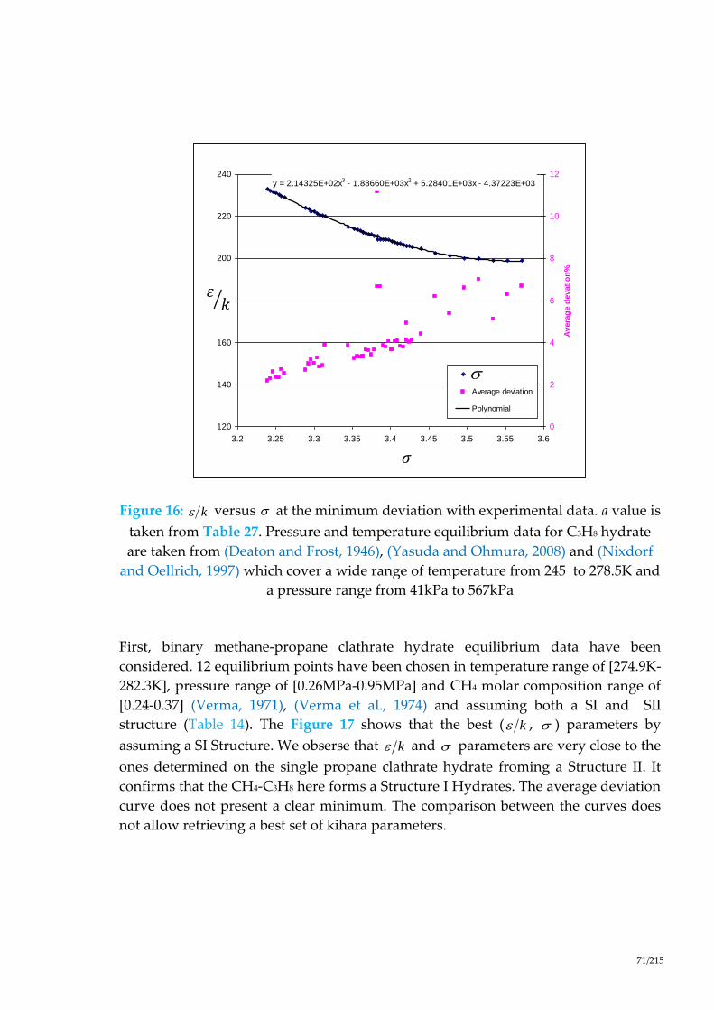
71/215


taken from Table 27. Pressure and temperature equilibrium data for C3H8 hydrate

are taken from (Deaton and Frost, 1946), (Yasuda and Ohmura, 2008) and (Nixdorf

and Oellrich, 1997) which cover a wide range of temperature from 245 to 278.5K and

a pressure range from 41kPa to 567kPa

First, binary methane-propane clathrate hydrate equilibrium data have been

considered. 12 equilibrium points have been chosen in temperature range of [274.9K-

282.3K], pressure range of [0.26MPa-0.95MPa] and CH4 molar composition range of

[0.24-0.37] (Verma, 1971), (Verma et al., 1974) and assuming both a SI and SII

structure (Table 14). The Figure 17 shows that the best ( k , ) parameters by

assuming a SI Structure. We obserse that k and parameters are very close to the

ones determined on the single propane clathrate hydrate froming a Structure II. It

confirms that the CH4-C3H8 here forms a Structure I Hydrates. The average deviation

curve does not present a clear minimum. The comparison between the curves does

not allow retrieving a best set of kihara parameters.

k

y = 2.14325E+02x3 - 1.88660E+03x

2 + 5.28401E+03x - 4.37223E+03

120

140

160

180

200

220

240

3.2 3.25 3.3 3.35 3.4 3.45 3.5 3.55 3.6

0

2

4

6

8

10

12

Avera

ge d

evati

on

%

Average deviation

Polynomial

k

𝜀𝑘ൗ

𝜎

72/215


taken from Table 27. Pressure and temperature equilibrium data for CH4-C3H8

hydrate are taken from (Verma et al., 1974) and (Verma, 1974).

Figure 18 and Figure 19 show another tentative to retrieve the propane kihara

parameters by doing an optimisation based on a Xe-C3H8 gas mixture, respectively

by assuming that Xe-C3H8 gas mixture forms a SII and SI Structure. The literature

data concerns only one equilibrium point from (Tohidi et al., 1993) but it gives not

only the pressure, temperature, gas composition in the gas phase, but also the gas

composition in the hydrate phase. It is then possible to calculate a mean deviation

not only based on the deviation between the experimental and calculated pressure,

but also on the hydrate phase composition.

Xe is a Structure II former, as well as C3H8 . If we assume that the gas mixture forms

a Structure II (Figure 18), we observe that the ( k , , F) curves of the pure propane

and Xe- C3H8 mixture does not present any intersection points. It is a different

situation from Figure 17 where the ( k , ) curves of the pure propane and CH4-

C3H8 mixture are identical and provide an infinite set of equivalent ( k , ) values.

In this case both pure propane as a Structure II former and CH4-propane as a

Structure SI former equilibria can be simulated. In the case of Xe-propane mixture,

there is no ( k , ) value which allows simulating both the equilibrium of pure

propane as a Structure II former and Xe- C3H8 as a Structure SII former. But, if we

assume that the Xe- C3H8 mixture forms an unexpected Structure I hydrate (Figure

19), it becomes possible to find a unique solution for ( k , ) which satisfies both

the simulation of the pure C3H8 and Xe- C3H8 mixture.

k

y = -4.27003E+01x3 + 7.25956E+02x

2 - 3.56206E+03x + 5.60359E+03

120

140

160

180

200

220

240

3.2 3.25 3.3 3.35 3.4 3.45 3.5 3.55 3.6

0

1

2

3

4

5

6

7

8

9

10

Avera

ge d

evati

on

%

Optimisation from single C3H8 gas

Optimisation from binary CH4-C3H8 mixture

Average deviation

Polynomial ( Optimisation from binary CH4-C3H8

mixture)

k

𝜀𝑘ൗ

𝜎

73/215

Figure 18 : versus at the minimum deviation with experimental data. SII is

assumed. a value is taken from Table 27. Pressure and temperature equilibrium data

for Xe- C3H8 hydrate is taken from (Tohidi et al., 1993).

Figure 19: versus at the minimum deviation with experimental data. SI is

assumed. a value is taken from Table 27. Pressure and temperature equilibrium data

for Xe-C3H8 hydrate is taken from (Tohidi et al., 1993).

k

k

120

140

160

180

200

220

240

3.2 3.25 3.3 3.35 3.4 3.45 3.5 3.55 3.6

0

5

10

15

20

25

30

35

40

Avera

ge d

evati

on

%

Optimisation from single C3H8 gas, SII is assumed

Optimisation from binary Xe-C3H8 mixture, SII is assumed

Average deviation Xe-C3H8 mixture

k

𝜀𝑘ൗ

𝜎

y = 1.58227E+03x3 - 1.47386E+04x

2 + 4.56928E+04x - 4.69554E+04

120

140

160

180

200

220

240

3.2 3.25 3.3 3.35 3.4 3.45 3.5 3.55 3.6

0

5

10

15

20

25

30

35

40

45

50

Avera

ge d

evati

on

%


Optimisation from binary Xe-C3H8 mixture, SII is assumed

Average deviation

Polynomial ( Optimisation from binary Xe-C3H8 mixture, SII is

assumed)

k

𝜀𝑘ൗ

𝜎

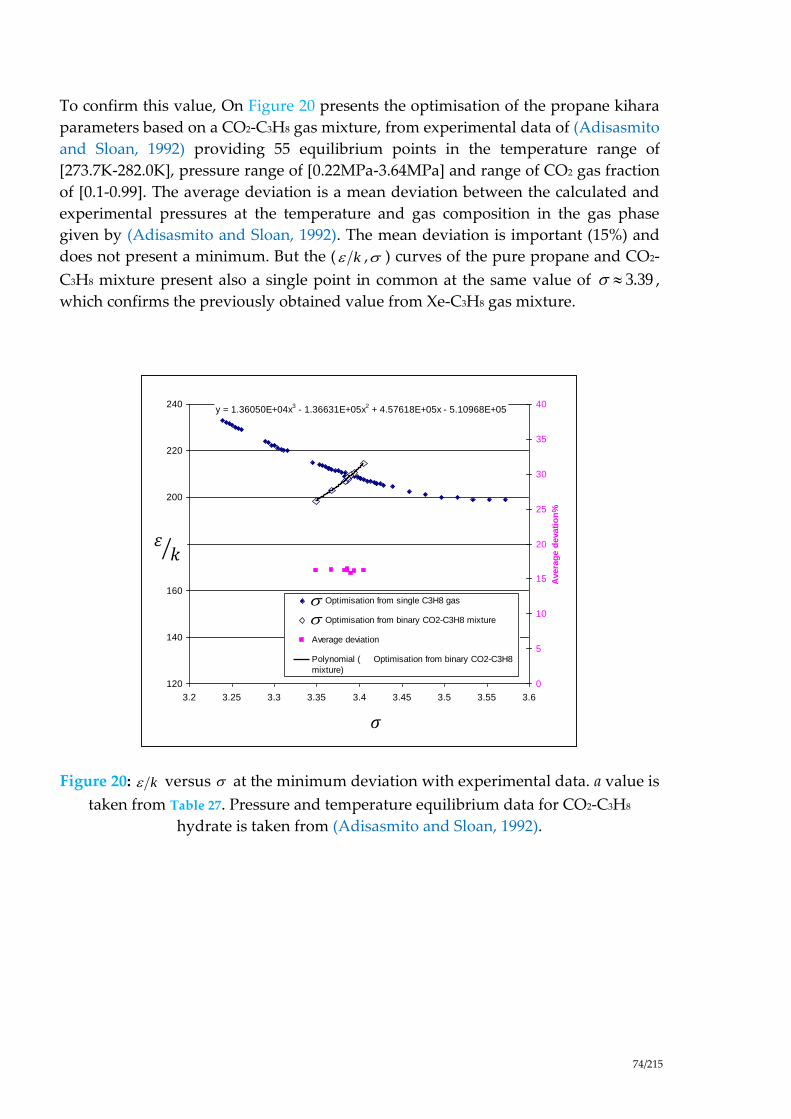
74/215

To confirm this value, On Figure 20 presents the optimisation of the propane kihara

parameters based on a CO2-C3H8 gas mixture, from experimental data of (Adisasmito

and Sloan, 1992) providing 55 equilibrium points in the temperature range of

[273.7K-282.0K], pressure range of [0.22MPa-3.64MPa] and range of CO2 gas fraction

of [0.1-0.99]. The average deviation is a mean deviation between the calculated and

experimental pressures at the temperature and gas composition in the gas phase

given by (Adisasmito and Sloan, 1992). The mean deviation is important (15%) and

does not present a minimum. But the ( k , ) curves of the pure propane and CO2-

C3H8 mixture present also a single point in common at the same value of 3.39 ,

which confirms the previously obtained value from Xe-C3H8 gas mixture.


taken from Table 27. Pressure and temperature equilibrium data for CO2-C3H8

hydrate is taken from (Adisasmito and Sloan, 1992).

k

y = 1.36050E+04x3 - 1.36631E+05x

2 + 4.57618E+05x - 5.10968E+05

120

140

160

180

200

220

240

3.2 3.25 3.3 3.35 3.4 3.45 3.5 3.55 3.6

0

5

10

15

20

25

30

35

40

Avera

ge d

evati

on

%


Optimisation from binary CO2-C3H8 mixture

Average deviation

Polynomial ( Optimisation from binary CO2-C3H8

mixture)

k

𝜀𝑘ൗ

𝜎

75/215

Table 28: Kihara parameters, after optimisation from experimental data with the

GasHyDyn simulator, implemented with reference parameters from Table 25

(Dharmawardhana et al., 1980) and Table 26.

Gas

k

a

CO2 178.21(*) 0.6805(+) 2.873(*)

CH4 166.36(*) 0.3834(+) 3.050(*)

C2H6 177.46(*) 0.5651(+) 3.205

C3H8 209.20(*) 0.6502(+) 3.390(*)

(*)-regressed from experimental data,

(+)-from (Sloan, 2005, 1998),

()-(Barrer and Edge, 1967a, 1967b)

76/215

77/215

5. HYDRATES UNDER NON EQUILIBRIUM CONDITIONS

5.1. INTRODUCTION

The laboratory has faced during the last decade experimental data, generally from

complex gas mixtures, which can hardly be modeled using the classical

thermodynamic approach given in the previous chapter (§3 Page 35).

A new approach has been attempted to give a fundamental explanation by re-

considering the (van der Waals and Platteeuw, 1959), which is fundamentally a

kinetic approach, but at equilibrium, where the hydrate finds its equilibrium as the

rate of enclathration of new species at its surface is equal to the rate of desorption of

the same species.

This approach has been extended by (Herri and Kwaterski, 2012) to non equilibrium

conditions that is to say when the fugacities of components in all the phases are not

equal, giving a driving force to start the elementary steps of the cristallisation.

Understanding the crystallization processes, especially nucleation and growth, are

essential in the modelling.

The historical model of (Volmer and Weber, 1926a) (§5.4.1) is an approach from the

thermodynamic collectivity where the kinetics is understood as an energetic barrier

to cross away. Kashchiev and Firoozabadi on their side (§5.4.2) (Kashchiev and

Firoozabadi, 2003, 2002a, 2002b) have applied to hydrates the backroung of the

collectivity that considers nucleation as a continuous mechanisms of clusters

aggregations considered individually as reactions. In the end, the collectivity of

chemical engineers (§5.4.3) has developed correlations to implement the nucleation

in a simple way in complex crystallization models.

But whatever the approach, each of the models define a driving force, as a

temperature difference, or a pressure ratio, or a concentration profile in between the

actual operative conditions and the equilibrium conditions. Based on an expression

of the driving force given as a concentration grandiant at the vincinity of the

growing particles, we conclude this chapter (§5.5) by enlighting that clathrate

hydrates, because they are non defined compounds, can encapsulate chemicals at a

composition that is not constrained by thermodynamics, but constrained by mass

transfers.

In the end, the composition of gas hydrates is geometric depending on the reactor in

which is operated the crystallization.

This chapter presents reviews of the elementary steps of the crystallization, and the

models given by the collectivity working in this field. Especially, theory of mass

transfer phenomena, nucleation and crystal growth are presented.

78/215

5.2. GENERALITIES ABOUT THE CRYSTALLIZATION OF GAS HYDRATES

The simplest situation corresponds to the crystallization of gas hydrate in a single

liquid phase, composed of pure water. In this case, gas molecules have to cross only

the gas/liquid interface, and the bulk phase.

If the reaction is operated in a stirred reactor, or a bubble reactor, the bulk solution

can be considered as homogeneous. Supersaturation ratio is defined as S=C/Ceq in

which C is the concentration in dissolved gas and Ceq is the equilibrium

concentration. We define supersaturation for each gas component. Three zones can

be distinguished as pointed by (Vysniauskas and Bishnoi, 1983):

Figure 21: Schematic of the concentration profiles in the environment of a particle in

a liquid bulk

- The first zone is the interface film layer. In the investigated system, its

thickness is about tens of micrometer. Because of the high supersaturation level of

this zone compared to the rest of the reactor, primary nucleation (§5.4) is particularly

active in the interfacial film which acts most of the time as a source of nuclei for the

bulk of the reactor.

- The second zone is the bulk zone in which the concentration is supposed to be

uniform. This zone is supposed to be the main place of the crystallisation process in

which we can find all the classical steps of growth, agglomeration, and secondary

nucleation.

- The third zone is the solid/liquid interface. The crystal is assumed to be

surrounded by two successive layers: an integration layer and a diffusion layer. The

integration layer is the region of volume in which a transition between the solid state

and the liquid state occurs. The integration layer can be considered as a solidification

layer.

First works were developed in Canada by (Vysniauskas and Bishnoi, 1983) and then

completed by (Englezos et al., 1987a, 1987b). The authors identified a mass transfer

Concentration in solute gasCeq Cb Cext

SupersaturationSextSb1

Interface film layerh

BulkParticle

Diffusion layer

Diffusion layer

H

79/215

limiting step at the gas liquid interface, or a growth rate limiting step at the vicinity

of the elementary particles, depending on the stirring rate. In 1994 (Per Skovborg

and Rasmussen, 1994; P. Skovborg and Rasmussen, 1994) analyzed again those

results and demonstrated that the limiting step remains the gas/liquid mass transfer,

whatever the stirring rate. This conclusion has been supported by (Herri et al.,

1999a) and (PIC et al., 2000) from experimental results obtained by using a new

particle size analysis tool (Herri et al., 1999b).

So, even in the simplest situation, the principal teams working on the subject

propose different approach. The degree of precision of the model is widely

dependent on the possibility to monitor the population of particles. So, this

modeling has been driven for decades by the development of new sensors adapted

to the high pressure conditions during crystallization. First experiments have

consisted in studying the gas consumption rate coupled with a population balance in

order to propose a model between the size/number of crystals, and the quantity of

gas consumed.

So, it can be said that, even in the simplest case consisting in crystallizing gas

hydrates in pure water, the authors doesn’t agree on the limiting step. A fruitful

reading is the reviewing from (Ribeiro Jr. and Lage, 2008).

5.3. MODELLING THE GAS/LIQUID TRANSFER IN A BATCH REACTOR

The Gas/Liquid transfer through the interface liquid film layer of thickness (Figure

21) is a first order law consistent with the well-known relation (Mehta and Sharma,

1971; Sridharan and Sharma, 1976):

, ,

i

i L i ext i bulk L Gr k a C C V (21)

1.ir mol s is the dissolution rate of component i, 1a m a is the mass transfer

surface area per unit of volume of liquid and 1.Lk m s the mass transfer coefficient,

-3

, mol.mi bulkC is the gaz component i concentration in the liquid bulk,

-3

, mol.mi extC is the interfacial concentration, and L GV is the liquid volume plus the

volume of gas that is eventually dispersed.

The Figure 22 plots the experimental determination of the i

Lk a value in the case of

methane.

80/215

Figure 22 : Influence of the stirring rate on the rate of methane dissolution in a

stirred batch reactor (Herri et al., 1999a)

5.4. MODELLING THE NUCLEATION

The nucleation is the process in which a new phase appears, here the crystal

clathrate hydrate (or semi clathrate hydrate). The nucleation is qualified as primary

if there is parent crystal. If a crystal is already present, it can help the nucleation

process, and the nucleation is qualified as secondary.

Both the primary and secondary nucleation are dependent on the level of

supersaturation of the reactants. The supersaturation ratio is defined as the ratio in

between the “concentration” of the reactant and the “equilibrium concentration”.

The composition of the liquid phase with respect to species is

characterised by a vector of generalised concentrations T

g1( , , )N . For chemical

engineering applications, especially applications concerning crystallisation processes

in liquids, liquid phase non-idealities are often neglected and the fugacity is replaced

by a concentration variable j . In this section, and in the remaining parts of this

manuscript, the variable will characterise the composition while the concentration

of the guest species is chosen to be the mole fraction x .

So, the supersaturation ratio is defined as the ratio between the mole fraction of

reactant j in the bulk ( , bulkjx ) and the mole fraction at equilibrium ( jx )

, bulkj

j

xS

x (22)

g1,...,j N

81/215

(Kashchiev and Firoozabadi, 2002a) have given different ways to express the driving

force for has hydrates from a rigorous approach based on thermodynamic

considerations (difference of chemical potentials). Then, (Noguera et al., 2006a,

2006b) have extended the work to precipitation, vapour condensation and

crystallization in the melt.

5.4.1 PRIMARY NUCLEATION FROM THE MODEL OF VOLMER AND WEBER (1926)

The original model of (Volmer and Weber, 1926a, 1926b, 1926c, 1926d) is the

reference model which gives the basement for the interpretation of the primary

nucleation mechanism. The original experiment deals with the nucleation of water

droplets in a supersaturated gas phase. (Volmer, 1929) considered that a local

fluctuation of density initiates a water droplet which size can be lower than critical

size, and that this droplet then dissociates. If its size is bigger than the critical size,

and the droplet continues to growth. This approach can be extrapolated to the

nucleation in solution, and especially the nucleation of clahtrates hydrates.

The solution is a liquid solution of water, and gas in solution, here called A. Wn is the

hydratation number. The liquid water molecules and the gas molecules A can

associate to form a cluster:

2 2w

w nn

n A n H O A H O

liquid cluster

(23)

𝑛 is the number of A molecules which aggregate with water to form a cluster. The

formation of the cluster is accompanied with a variation of the Gibbs energy nG ,

corresponding to the formation of the new volume nV , and a new interface of surface

nS of:

liq to solid nn n

cluster

VG S

(24)

The first term is equal to the difference ∆𝜇 between the chemical potentials of n

nucleation units in solution and in the solid. The second term is a surface term,

proportional to the particle surface energy. cluster is the molar volume of the cluster,

Wn

82/215

the volume of AvN (number of Avogadro) unities of cluster 2wn

A H O . It is equal to

w Wn where

W is the molar volume of clathrate per mole of water molecule.

is the partial Gibbs energy. It can be expressed in the following form:

WA Wclustern (25)

The chemical potential of solute A is:

0 lnA A A

RT a (26)

In a first approximation, the activity coefficient of solute A in solution can be

evaluated by its mole fraction , bulkAx .

The chemical potential of water in liquid solution is:

0 lnW W W

RT a (27)

In a first approximation, the activity of water is , bulk1 Ax , and in a second

approximation, equal to 1.

The chemical potential of the cluster is assumed to be the value at the reference state:

0

cluster cluster (28)

So, finally:

0 0

ul

0

, b klnA Wcluster W An xRT (29)

And at thermodynamic equilibrium

0 0 00 lnA Wcluster AWn RT x (30)

And finally, combining Eq. (29) and Eq. (30), it gives:

83/215

, bulkln ln

A

A

RT Rx

Tx

S (31)

After combination of Eq. (24) and Eq. (31), we obtain a general expression to

calculate the variation of the Gibbs energy during the formation of a cluster of n

basic unities :

lnliq to solid

n n n

W W

RTG V S S

n

(32)

If the cluster is assumed to be spherical, and diameter l :

v A

3

A v6n Wcluster W

N N

n nV l n

(33)

v

3

A

1

6W W

N

nl n

(34)

A

2

v

123 3

2 2 32

Av

6 136

W Wn W W

nS n n n

NN

(35)

Av Av

21

332 2ln . 36

W W

liq to solid

n SN

n nG RT n

N

(36)

Figure 23 shows the variation of the Gibbs energy of formation, in respect to the

value of the supersaturation. The first observation is the shape of each curve, with a

maximum. It depicts the existence of a cluster critical size. Below the value of the

critical size, the clusters which are formed are not stable, because their tendency is to

decrease their size to diminish their Gibbs energy, and dissociate. But, following the

interpretation of (Volmer and Weber, 1926a), the fluctuations which generate

clusters with a size above the critical allow to form stable crystals. In fact, the clusters

can continue to grow by decreasing their value of Gibbs energy.

The size of the critical cluster is given by:

2wn

A H O

84/215

0nd G

dn

(37)

* 4l

g

(38)

From Eq. (32) and assuming cluster to be spherical, we got:

*

44

ln

W Wn

Sl

RT

(39)

The Eq. (39) shows that the critical size decreases as the supersaturation increases.

The maximum (or critical) Gibbs energy, corresponding to the critical size, is a

barrier of formation. From Eqs. (32 - 35), we can calculate its value:

3 2 2

*

homogeneous 2 2 2

16

3 ln

W Wn

GR T S

(40)

On Figure 23, we can observe the decrease of the critical size Eq. (39) and decrease of

the maximum Gibbs energy Eq. (40) as the superstation is increased.

85/215

Figure 23 : Shape of the Gibbs energy function during formation of a cluster of n

entities, depending on supersaturation (Herri, 1996)

From Eq. (40), (Volmer and Weber, 1926a) has proposed to consider the maximum

Gibbs energy as an activation energy. As a consequence, it is possible to propose a

kinetic interpretation of Eq. (40), and to give a simple expression of the nucleation

rate BI (i.e. the number of nuclei produced per unit volume and unit time) under the

form:

3 2 2

31

*

3 21

16e

3 lnxp exp

W W

IB k kR T S

G

T

n

R

(41)

in which k1 is a constant.

The rate of primary nucleation can not be measured experimentally easily. In fact,

the size of the critical nuclei, about tens of nanometers, remains inaccessible to the

majority of particle sizers.

But, the nucleation rate can be indirectly quantified because it is inversely

proportional to the induction time. The induction time is the duration between the

moment at which the solution is considered to be supersaturated, and the moment at

which the first crystals are observed:

86/215

3 2 2

3 3 2

16

3e

lnxp

W W

ind

n

R Tt

S

(42)

For gas hydrate in pure water, the supersaturation can be controlled via the

operative pressure. The following Figure 24 shows the shape of the induction time as

function of the operative pressure. The shape is very typical. It shows the existence

of the minimum supersaturation under which the operator has to wait an infinite

time before observing the nucleation, but above which the nucleation time decreases

and becomes null.

From an experimental point of view, Eq. (42) explains the fact that the nucleation can

be experimentally observed, only if a minimum level of supersaturation is applied.

Figure 24: Induction time versus supersaturation during nucleation of methane

hydrate in pure water, at 1°C (Herri et al., 1999b)

From Eq. (42) and Figure 24, it is possible to estimate the value of the interfacial

energy -25.3mJ.m between the hydrate and the liquid water. This value is inferior

to the value of the interfacial energy between ice and liquid water ( -228mJ.m ).

The difference can be a true difference in respect to physical difference between the

ice and the clathrate hydrate. But also, it can be explained from the consideration

that nucleation is not homogeneous, but heterogeneous. In a heterogeneous

mechanism of nucleation, the formation of the critical nuclei takes place at an

interface. It can be a solid surface such as the wall of the reactor, or a dust. Also, it

can be a gas/liquid interface. The shape of the critical nuclei moves from a spherical

87/215

geometry (homogeneous nucleation) to a complex form, such as a cap-shaped cluster

(heterogeneous nucleation at a solid interface), or a lens-shaped cluster

(heterogeneous nucleation at a gas/liquid interface). The shape depends on the

relative interfacial energy between the phases. The respective values fix the

angles at the heterogeneous junctions in respect to the Young equation (Eqs. 44, 46

and 47). The different situations are summarised in Table 29, from an original work

of (Vysniauskas and Bishnoi, 1985) summarised and extended by (Kashchiev and

Firoozabadi, 2002a, 2002b).

The presence of an interface results in a decrease of the critical Gibbs energy. This

decrease can be quantified under the form of a factor between 0 and 1 (Eqs. 45

and 48).

* *

heterogeneous homogeneousG G (43)

*

homogeneousG is given in Eq. (40).

In the case of a nucleation on a solid surface (Table 29 case b) with a formation of a

cap-shaped cluster, the shape of the value of is given on Figure 25 as a function of

the contact angle.

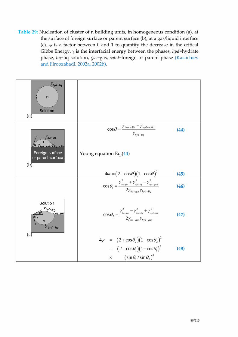
88/215

Table 29: Nucleation of cluster of n building units, in homogeneous condition (a), at

the surface of foreign surface or parent surface (b), at a gas/liquid interface

(c). is a factor between 0 and 1 to quantify the decrease in the critical

Gibbs Energy. is the interfacial energy between the phases, hyd=hydrate

phase, liq=liq solution, gas=gas, solid=foreign or parent phase (Kashchiev

and Firoozabadi, 2002a, 2002b).

(a)

(b)

cos

liq solid hyd solid

hyd liq

(44)

Young equation Eq.(44)

2

4 2 cos 1 cos (45)

(c)

2 2 2

1cos2

liq gas hyd liq hyd gash

liq gas hyd liq

(46)

2 2 2

2cos2

liq gas hyd liq hyd gas

liq gas hyd gas

(47)

2

2 2

2

1 1

3

1 2

4 2 cos 1 cos

2 cos 1 cos

sin / sin

(48)

89/215

Figure 25: The factor versus angle according to Eq. (45)

If the formulation of (Volmer and Weber, 1926a) has the advantage of simplicity and

can depict many experimental facts such the induction time and it is based on a

simplified assumption. It considers that primary nucleation is the event which

transforms instantaneously of volume of solution from a state (here the liquid with

supersaturated gas) to another state (the hydrate phase). For the specific case of gas

hydrates, a rigorous approach of primary nucleation from Volmer and Weber theory

has been proposed by (Kashchiev and Firoozabadi, 2003).

5.4.2 PRIMARY NUCLEATION FROM A RIGOROUS KINETIC APPROACH

The modelling of primary nucleation can be considered from another point of view.

It is possible to consider that nucleation is a continuous process, similar to

agglomeration or polymerisation, during which the nuclei are growing step by step

to reach a stable size (Becker and Döring, 1935; Cournil and Gohar, 1989; Dunning,

1955; Farkas, 1927; Kashchiev, 1984; Katz and Spaepen, 1978; Katz and Wiedersich,

1977; Zettlemoyer, 1969).

The nucleation is observed as a significant flow of new particles can be detected. The

existence of clusters of molecules has been proven experimentally in gas. But the

presence of such clusters in liquid solutions is remained a postulate for years. The

more advanced works have been developed in the team of (Myerson and Lo, 1990)

and also (Mohan et al., 2000). Today, the existence of clusters in supersaturated

solutions or in non saturated solutions has showed evidences: new Raman

frequencies appearing in supersaturated solution, concentration gradients in

90/215

stagnant zones induced by the differential sedimentation of clusters, drop of the

diffusion constant in electrolytes or non electrolytes solutions.

The size of the clusters has been measured to be 2, 50 and 100 elementary units

respectively in Glycine solution, potassium sulphate solution and citric acid solution.

Figure 26: Association of clusters

2 2

2 2 22

2 2 21

Equilibrium1

Equilibrium 2

...

...

Equilibrium M

w

w w w

w w w

w n

n n n

n n nM M

A n H O A H O

A H O A H O A H O

A H O A H O A H O

(49)

This approach needs to be completed with three remarks

1) The agglomeration between clusters is supposed to be low enough to be

neglected,

0

2 2 20w w wn n n

M N M N

A H O A H O A H O

(50)

The opposite reaction of dissociation of a cluster into two clusters is also

supposed to be negligible.

2) The notion of nucleation rate is defined as a reaction. The nucleation is a

succession of condensations with individual rates:

1

12 2 2

1 1

i i

w w wi i

a a

n n nd di i

A H O A H O A H O

(51)

91/215

The system is completely defined if the constants of condensation ( ia ) and

dissociation ( id ) are defined. The condensation constants ( ) can be

determined from simple kinetic consideration (Farkas, 1927). Unfortunately,

there is no model available to evaluation the constant of dissociation ( ). The

problem can be partially solved by introducing a stationary reference state:

10 i iJ J (52)

iJ is the number of cluster of i unities which condensate (per unit of time and

volume) to form a cluster of (i+1) unities. Equation Eq. (52) implies that the

concentration of clusters is constant. (Kashchiev, 1984) showed that the

establishment of this stationary regime is very rapid.

3) The nucleation rate allows defining a nucleation time. It corresponds to the

duration for the biggest clusters of size M to reach a size and a concentration

that could be detected by the operator.

Each cluster is supposed to be at thermodynamic equilibrium. In the following

equation, the elementary cluster unit 2wn

A H O is renamed as H .

1

with 2n

cluster cluster

i H H n M (53)

Av

.i

HH

n

N (54)

Av

1

,

,

nH bulk

nn N

H bulk

xK

x

(55)

iK is a constant of equilibrium:

,0

exp n

cluster to cluster

n

GK

RT

(56)

ia

ia

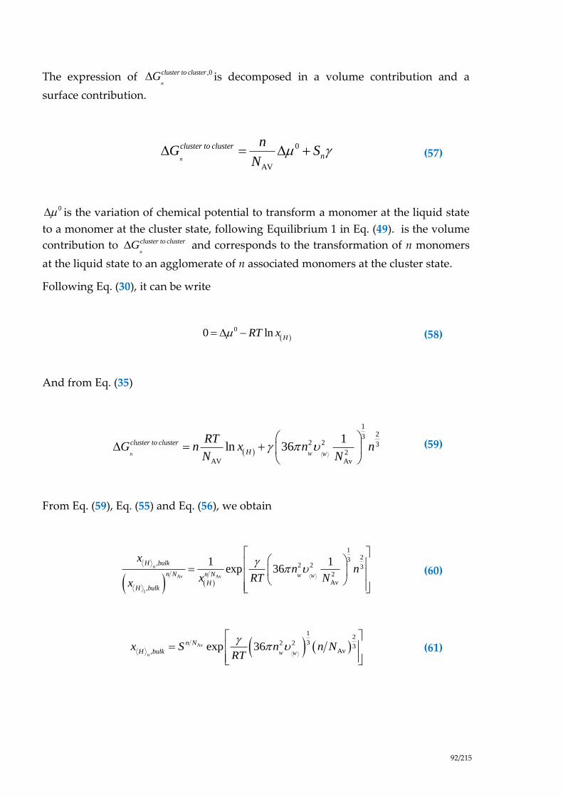
92/215

The expression of ,0

n

cluster to clusterG is decomposed in a volume contribution and a

surface contribution.

0

AVn

cluster to cluster

n

nG S

N (57)

0 is the variation of chemical potential to transform a monomer at the liquid state

to a monomer at the cluster state, following Equilibrium 1 in Eq. (49). is the volume

contribution to n

cluster to clusterG and corresponds to the transformation of n monomers

at the liquid state to an agglomerate of n associated monomers at the cluster state.

Following Eq. (30), it can be write

00 lnH

R xT (58)

And from Eq. (35)

123

2 2 32

AV Av

1ln 36

n W W

cluster to cluster

Hx

RTG n n n

N N

(59)

From Eq. (59), Eq. (55) and Eq. (56), we obtain

Av Av

1

123

, 2 2 32

Av,

1 1exp 36n

W W

H bulk

n N n N

H b lH

u k

xn n

RT Nx x

(60)

Av

12

32 23

Av,exp 36

W Wn

n N

H bulkx S n n N

RT

(61)

93/215

Figure 27: Molar fraction of clusters at equilibrium. The index n refers to the number

of elementary units of the cluster. S is the value of the supersaturation

The Figure 27 shows the shape of the concentration profiles (here the molar fraction)

of the cluster in the supersaturated solution:

- For the unsaturated solution, up to a supersaturation of 1, the concentration

profile is continuously decreasing,

- For the supersaturation above the value of 1, the concentration profile is

firstly decreasing down to a plateau, and then increasing. The value of the

concentration at the plateau increases as the supersaturation increases. It

depicts the fact that the concentration of clusters increases as the

supersaturation is increased.

5.4.3 PRIMARY NUCLEATION FOR CHEMICAL ENGINEERS

It needs to be said the modelling of nucleation remains incomplete in respect to

many facts: 1) the extrapolation of macroscopic thermodynamic to small clusters

encounters a limit in the definition of the elementary energetic constants such as

specific energetic surface, 2) it is difficult to observe experimentally the nucleation in

respect to the small size of nuclei, 3) the nucleation is generally stochastic.

So, it is useful to express the primary nucleation in a simplified analytical form,

taking into account the driving force directly, (Cournil and Herri, 2003) (Eq. 62) or

indirectly from another variable that is also dependent on the driving force, for

example the growth rate G, (PIC et al., 2000) (Eq. 63):

94/215

1

1 1s

IB S (62)

1

g

IB G (63)

In such formulations, s1 and g are adjustable parameters

5.4.4 SECONDARY NUCLEATION

During the crystallization, after the appearance of the first crystal, new mechanisms

of nucleation are introduced in respect to the presence of parent crystals. Nucleation

can be observed at level of supersaturation in which primary nucleation is not

possible. These new mechanisms of nucleation are qualified as secondary nucleation.

(Botsaris, 1975) proposes to distinguish three different cases:

- Initial breeding: In industrial crystallization, it is useful to force the nucleation

by introducing parent crystals in the supersaturated solution. After

introduction, it is observed a sudden and massive nucleation induced by the

crystal dusts dispersed in the solution from the parent crystal surface.

- Catalytic nucleation: the parent crystal, under growing, can generate some

clusters or nuclei at their surface. If they are scarpered from the surface, for

example in reason of the local turbulence or chocks in between particles, they

constitute sorts of elementary pieces that can reach a stable size more easily.

Also, the presence of the parent crystal is a surface on which the primary

nucleation can be activated from a catalytic mechanism. The catalytic

nucleation is only possible in a supersaturated solution.

- Attrition: the reactor in which is operated the crystallisation is a stirred

volume, with mechanical chocks in between the particles, or in between the

particles and walls or stirrer blades. The particles can be broken into different

pieces. If the crystal is broken in pieces of comparable sizes, the process is

qualified as fragmentation. If very small particles are generated, the process is

qualified as attrition, and can be regarded as a generation of new nuclei.

It is difficult to propose a mechanism for each situation. (Mersmann et al., 1992)

proposes to model the secondary nucleation under a general formulation:

3

1p s w

II pB S S (64)

95/215

5.5. MODELLING THE GROWTH

The classical approach of (van der Waals and Platteeuw, 1959) provides a

description of the thermodynamics of equilibrium involving clathrate hydrate

phases. In this approach, the encapsulation of gas molecules in the empty cavities is

described similarly to the adsorption of molecules on a two dimensional surface. The

model assumptions lead to a Langmuir type of equation for describing this

“adsorption” of guest species onto the empty lattice sites.

During crystallisation (here in a liquid system), the crystal is assumed to be

surrounded by two successive layers: an integration layer and a diffusion layer. The

integration layer is the region of volume in which a transition between the solid state

and the liquid state occurs. Following the approach of (Svandal et al., 2006), the

integration layer can be considered as a solidification layer. It is described by means

of the scalar phase field and a composition variable. At the interface between the

solid and the integration layer, the scalar phase field assumes the value 1 (solid

state). Furthermore, local equilibrium is assumed. The local equilibrium composition

is characterised by the set of mole fractions jx for all gj S . Then, in the direction of

the second interface, between the integration layer and the diffusion layer, the scalar

field varies from 1 (solid state) to 0 (liquid state), and the composition varies from

to , intjx . The whole model is described by (Herri and Kwaterski, 2012) and hereafter.

In contrast to (Svandal et al., 2006), a model description of the profiles of the scalar

phase field or the composition variables is not given in this work. We only assume

that they exist and simplify the problem by introducing Eq. (77) which is described

below.

The modelling of the diffusion layer is easier, since it is a liquid, though

continuous, phase throughout. The composition varies from at the interface

between the integration layer and the diffusion layer to , bulkjx at the interface

between the diffusion layer and the liquid bulk phase. A schematic representation of

the different regions surrounding the hydrate phase under formation conditions is

given in Figure 28.

jx

, intjx

96/215

Figure 28 : Elementary steps of gas integration in the vicinity of the growing hydrate

surface (Herri and Kwaterski, 2012).

In such a system, the different species j are enclosed by the sites in proportion to

their relative affinity. The rate of enclathratation, , ej ir , is directly proportional to the

product of the mole fraction , intjx of j and the fraction of empty cavities, 1 i ,

according to

, e , , e , int (1 )j i x ji j ir k x (65)

where , , ex jik is the corresponding kinetic rate constant of enclathration of species j in

a cavity of type i,. The subscript x at the symbol k refers to the mole fraction as the

particular concentration variable chosen for .

The liberation of guest species from the cavities of type i due to the

declathration process can be described by the following rate law

, d , dj i j i j ir k (66)

In other words, the corresponding molar rate , dj ir is directly proportional to the

occupancy factor j i , i.e. the fraction of cavities i which are filled with guest species

.

As a result, we can define a local flow rate of component j which results from the

unbalance between adsorption and desorption:

Hydrate crystal growing at a growth rate G.

Simultaneous enclathration and declathration

of different guest species j

in different types of cavities i

Diffusion layer

, ej ir , dj ir

Integration layer

jx

, intjx

, bulkjx

G1([ ] ms )G

j

j

97/215

, e , d , , e , int , d(1 )ji ji ji x ji j i ji jiF r r k x k (67)

Eq. (67) can be rewritten as:

, , e

, e , d , d , int

, d

(1 )x ji

j i j i j i j i j j

j i

kF r r k x

k

(68)

Particular case of equilibrium

At equilibrium, 0j iF , and the following relation is derived from Eq. (68), holding

for all gj S , taking into account that , bulk , intj j jx x x :

, , e

, d

, d

(1 ) 0x ji

j i j j

j i

kk x

k

(69)

With the Langmuir constants ,x jiC defined as the ratio between the rate of

enclathration and declathration according to:

, , e

,

, d

x j i

x j i

j i

kC

k (70)

Eq. (69), can be re-written as:

cav g

, (1 ) 0x ji j i j ii S j S

C x (71)

Summing up Eq. (71) over all guest species leads to

g

g g

,

, ,

11

1 1

x j i j

j S

i i

x j i j x j i j

j S j S

C x

C x C x

(72)

Finally, by inserting Eq. (71) into Eq. (72), the following relation is derived for j i

98/215

g

,

,1

x j i j

j i

x j i j

j S

C x

C x

(73)

5.5.1 ENCLATHRATION DURING CRYSTALLISATION

The surface of crystal is supposed to be covered with cavities under formation,

which can be regarded as “opened cavities” or active sites. They are assumed to

cover the surface and we can define a concentration i (number of moles of active

cavities of type i per unit of surface area, 2[ ] molmi ). Each type of opened cavity

i is exposed to a rate j iF (mole of component j /mole of cavity of type i /unit of time).

During the growth of the crystals, the rate by which the gas molecules j (mole per

unit of time) are incorporated into the cavities of the newly created volume is given

by:

j i i sF A (74)

Where sA denotes the total surface area of the growing crystals. The crystal is

assumed to grow at a rate G ( 1[ ] msG ). The increase in volume of the quantity of

solid newly formed per element of time dt is given by

s

dVGA

dt (75)

The volume of the newly formed solid is composed of water molecules which build

a network of cavities of different types i. Their molar volumetric concentration is ic

(moles of cavity of type i per unit of volume) and they are occupied by gas molecules

of type j. The occupancy is given by j i (mole of component /mole of cavity ). The

flow rate by which the gas molecules j (mole per unit of time) are incorporated in the

cavities of the new volume is:

si j i i j i

dVc c GA

dt (76)

From Eq. (74) and Eq. (76), it follows for all cavi S and all that

j i

gj S

99/215

i j i i j iF c G (77)

Summing up Eq.(77) over all leads to

i i i iF c G (78)

A general consideration to be taken into account is the following relationship that for

each cavity , but for two different molecular adsorbents and j , is obtained from

Eq. (77):

g g cav

j i j i j i j i

j S j S i Sj i j i j i j i

F F F

F

(79)

From Eq. (79) it follows that a characteristic constant ia can be defined according to:

g cav

j i

ij S i S

j i

Fa

(80)

After summation over all guest species j , the total flow rate iF of guest molecules

arriving at the cavity i under construction is

g g g

ii j i i j i i j i i i i

j S j S j S i

FF F a a a a

(81)

Thus, with Eq. (78) it can be found from Eq. (81) that for all cavi S

ii

i

ca G

(82)

gj S

i j

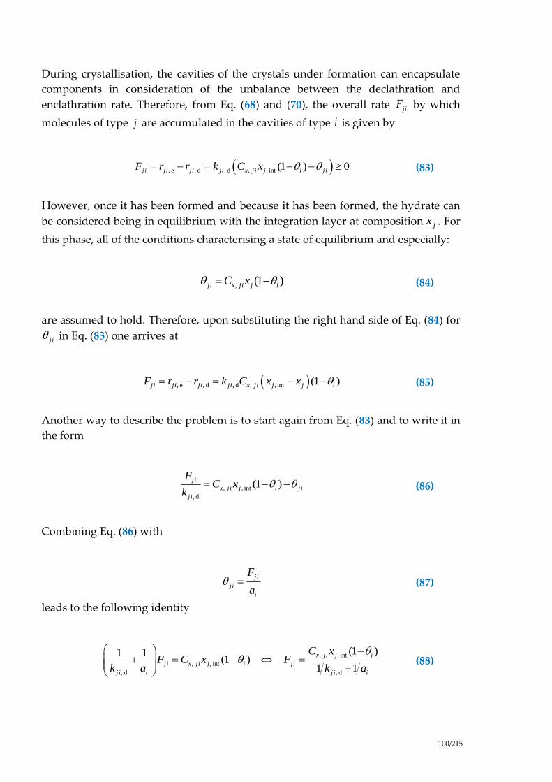
100/215

During crystallisation, the cavities of the crystals under formation can encapsulate

components in consideration of the unbalance between the declathration and

enclathration rate. Therefore, from Eq. (68) and (70), the overall rate j iF by which

molecules of type j are accumulated in the cavities of type i is given by

, e , d , d , , int (1 ) 0ji ji ji ji x ji j i jiF r r k C x (83)

However, once it has been formed and because it has been formed, the hydrate can

be considered being in equilibrium with the integration layer at composition jx . For

this phase, all of the conditions characterising a state of equilibrium and especially:

, (1 )j i x ji j iC x (84)

are assumed to hold. Therefore, upon substituting the right hand side of Eq. (84) for

j i in Eq. (83) one arrives at

, e , d , d , , int (1 )ji ji ji ji x ji j j iF r r k C x x (85)

Another way to describe the problem is to start again from Eq. (83) and to write it in

the form

, , int

, d

(1 )j i

x j i j i j i

j i

FC x

k (86)

Combining Eq. (86) with

j i

j i

i

F

a (87)

leads to the following identity

, , int

, , int

, d , d

(1 )1 1(1 )

1 1

x ji j i

j i x j i j i j i

j i i j i i

C xF C x F

k a k a

(88)

101/215

being valid for all and . The equality of Eq. (85) and Eq. (88) reads

, , int

, d , , int

, d1 1

x ji j

j i x j i j j

j i i

C xk C x x

k a

(89)

which is equivalent to

, int

, int

, d1

j

j j

j i i

xx x

k a

(90)

Eq. (90) has a strong consequence. The left member of the equality in Eq. (90) is a

driving force, expressed here by a difference of the mole fraction of the species to be

integrated in the structure under growing. This driving force is the same for any

cavities. It means that the right member of the equality in Eq. (90) is also

independent of the cavity. It can be stated more specifically that the ratio , dj i ik a is

independent of the nature of the cavity. Upon expressing ia by means of Eq. (82) in

terms of ic , i and G , the ratio , dj i ik a is given by

, d , dj i j i i

i i

k k

a Gc

(91)

The independence of of the nature of the cavity i gives rise to the definition

of a kinetic constant jk , which is to be regarded as an intrinsic kinetic constant of

component j

, d

ij j i

i

k kc

(92)

By expressing in Eq. (90) by means of Eq. (91) and (92) in terms of and G

and solving for jx , the following relationship is obtained

, int

1

j

j j

j

k Gx x

k G

(93)

gj Scavi S

, dj i ik a

, dj i ik a jk

102/215

It summarises the relations that allow for the calculation of the hydrate composition

as a function of the composition of the liquid phase in the vicinity of the growing

hydrate crystal. The expressions are dependent on the composition , intjx at the

interface between the integration layer and the diffusion layer.

To composition can be evaluated from a mass balance in Eq. (94) giving the

equality between the integration rate due to the Langmuir type of enclathration (lef-

hand-side), and the gas diffusion around (right-hand-side):

gcav

ws s , bulk , int

w

i j i j j jj S

i S

GA c d A x xM

(94)

Where , bulkjx is the mole fraction of j in the bulk phase, and jd ( 1[ ] msjd ) the

mass transfer coefficient of the guest species j around the crystal, respectively. w

and wM , respectively, stands for the density (3

w[ ] kg m ) and the molar mass (1

w[ ] g molM ) of the solvent (water), respectively. *

id can be estimated from a

classical correlation between the dimensionless Reynolds, Sherwood and Schmidt

numbers of/around the crystal particle (index “p”), pRe , pSh and Sc , as for example

by the one of (Armenante and Kirwan, 1989) which can be retained

0.52 1 3

p pSh 2 0.52Re Sc (95)

pSh

j

j

d l

D

, 4/3 1/3

pRel

, Sc

jD

(96)

In the equations compiled in Eq. (96), l is the diameter of the crystals under growing

and the kinematic viscosity of the liquid phase, approximated by the kinematic

viscosity of the pure solvent, i.e. water. jD ( 2 1[ ] m sjD ) denotes the diffusivity of

the gas in the solvent. It can be extrapolated from the value at a given temperature

by using the correlation of (Wilke and Chang, 1955) in which constjD T . is the

dynamic viscosity at temperature T , stands for the energy dissipation rate per unit

mass of the fluid, here water. For the case of a stirred reactor equipped with a four

blades impeller, the following relationship for is provided by (Baldi et al., 1978).

5 3

stirring rate impeller diameter

liquid volume (97)

103/215

Table 30: Occupancy factor of enclathrated molecules as a function of the

composition in the liquid phase. The equations of the right-hand column

are obtained from the classical Langmuir expressions from Eq. (73) (left

column) upon replacing jx by the expression of Eq. (93) (right column).

Thermodynamic

equilibriuma

Local equilibrium resulting from a kinetic

equilibriuma

j i

g

,

,1

x j i j

x j i j

j S

C x

C x

, int

1

j

j jj

k

Gx xk

G

g

, , int

, , int '

(1 )

1 (1 )

j x j i j j

j x j i j j

j S

K C x k G

K C x k G

i g

g

,

,1

x j i j

j S

x j i j

j S

C x

C x

g

g

, , int

, , int '

(1 )

1 (1 )

j x j i j j

j S

j x j i j j

j S

K C x k G

K C x k G

1 i

g

,

1

1 x ji j

j S

C x

g

, , int

1

1 (1 )j x j i j j

j S

K C x k G

a The Langmuir coefficient is usually calculated by using a modified Kihara approach in

which the mole fraction jx of the guest component j is replaced by the corresponding

fugacity jf . Expressing the relation between the Langmuir coefficients

,x jiC and ,f j i j iC C as

,x ji j ji iC x C f , an approximate relation can be derived for calculating as a function of j iC

by using a simplified version of Henry’s law in the form of , w m,exp( )j j H j jf x k pV RT , where

liquid phase non-idealities expressed by means of the activity coefficient as well as the

pressure dependence of m, jV , the partial molar volume of j at infinite dilution, are neglected.

In this relationship , wH jk is Henry’s constant of the guest species j in the solvent water at

the saturation pressure of the solvent. By proceeding in that way, the approximate relation

, , w m,exp( )x ji ji H j jC C k pV RT is obtained.

Thus, once numerical values for jk ( 1[ ] msjk ) and for G are assumed, the , intjx

values can be determined as the solution of the system of the N non-linear

equations Eq. (98). This set of equations is obtained by substituting the expressions

for of Table 30 into Eq (94).

,x jiC

j i

104/215

g

cav

g

, , int

, bulk , int

, , int

(1 )

1 (1 )

j x j i j j

i j j jj S

i S j x j i j j

j S

K C x KG c d x x

K C x K

(98)

with w

w

j jd dM

Where the quantity jd has the dimension of a molar flux and thus 2 1[ ] mol m sjd .

The last equation to be taken into account for completely solving the problem is a

relation expressing the hydrate stability. The subject of this work is not to describe

the physical model inherited from the model of (van der Waals and Platteeuw, 1959).

For more details on that issue, see in (Sloan, 1998; Sloan and Koh, 2007). A fruitful

reading could also be a previous study (Herri et al., 2011) which has motivated the

work presented in here. In fact, it focuses on the inter-dependency of internal

parameters (i.e. Kihara parameters versus reference state parameters) and points to

the difference between the experimental data from different laboratories.

The fundamental equation expressing the hydrate stability is deduced from

statistical thermodynamics. It demonstrates that the hydrates become stable once the

cavities are sufficiently filled, without considering the chemical nature of the

components.

cav

H

w ( , , )ln 1

β

i i

i S

T p

RT

(99)

In Eq. (99), R is the universal molar gas constant and is the vector of independent

occupancy factors. The summation is to be performed over all types of cavities (e.g.,

the two types of cavities, 512 and 51262 in case of a sI hydrate with a stoichiometry of 2

and 6, respectively, as shown in Table 1, counted by the index i . H

w

β is the

difference of the chemical potential of water in the hydrate phase and the chemical

potential of water in an hypothetical empty hydrate lattice, denoted as . It can be

calculated since, at equilibrium, the chemical potential of water in the solid phase

and in the liquid phase are equal. The difference between the chemical potential of

water in the liquid phase and in the -phase, L

w ( , )T p , is calculated by means of

the following relation originating from classical thermodynamics, explained in detail

in (Sloan, 1998; Sloan and Koh, 2007).

105/215

0 0

L LL Lm, w 0 m, ww w 0 0

2

0

L

w

( , ) ( , )( , , ) ( , )

ln ( , , )

pT

T p

H T p V T pT p x T pdT dp

RT RT RT RT

a T p x

(100)

In Eq. (100), 0T and 0p are reference values for temperature and pressure, taken to be 273.15 K and 0 MPa , respectively, whereas x denotes the vector of independent mole fractions in the liquid phase indicating the composition dependence of L

w

and L

wa , the latter of which stands for the activity of water in the liquid phase. L

m, w ( , )V T p denotes the difference in the molar volumes of water in the liquid and the -phase, respectively. The latter has been measured with high accuracy by (Stackelberg and Müller, 1951). The value of L

m, w 0( , )H T p can be expressed as temperature dependent according to (Sloan, 1998; Sloan and Koh, 2007). The last parameter of the equation is

L

w 0 0( , )T p . Numerical values published for this parameter show strong variations among different laboratories (Herri et al., 2011). Therefore, it needs to be selected with precaution when being used in calculations of the Langmuir coefficient together with Kihara parameters which are retained on the other hand (Herri et al., 2011). Once

L

w

is calculated, which in equilibrium is equal

to H

w

β , the hydrate composition needs to satisfy the identity given by Eq. (99). Hence, by eliminating i from Eq. (99) via the expression presented in Table 30, the growth rate G fulfils the equation

cav g

H, , intw ln 1

1

βj x j i j

i

i S j S j

K C x

RT K

(101)

Finally, the local equilibrium is defined when the values of and , intjx for all gj S

satisfy Eq. (98) and (101).

The calculation procedure is outlined in more detail in Figure 29. It is a double

convergence loop. In the first loop, an iteration is performed on the growth rate in

order to satisfy Eq. (101) describing the hydrate stability. From a physical point of

view, the G value is the value at which the structure can grow by incorporation of

solute gas to such an amount that is sufficient for stabilising the structure (i.e. the

cavities are filled to a sufficient extend). The relative proportion to which the

different gas molecules j are entering the structure is determined in the second

convergence loop which is an indirect consequence of the competition between the

diffusion rates around the crystals and integration rates in the structure. By this

competition the , intjx values are fixed.

Even for a system containing only a single hydrate forming component Aj , it can be demonstrated that the hydrate phase does not form at equilibrium. Eq. (99) along with the expressions presented in Table 30, can be written at kinetic

G

106/215

equilibrium, during crystallisation, and yields to Eq. (101), and after mathematical reformulation to Eq. (102). At thermodynamic equilibrium, Eq. (99) leads to Eq.(105)

cav cav

H, , intw

,

cryst

exp 1 11

i

i

βj x j i j

x j i j

i S i Sj

K C xC x

RT K

(102)

where the index “cryst” indicates that the properties are calculated during

crystallisation. jx is to be calculated from , intjx by means of Eq. (93). At equilibrium,

the following relation holds:

cav

H

w, , eq

eq

exp 1i

β

x ji j

i S

C xRT

(103)

On the other hand Eq. (100) becomes:

LL L L w

w cyst w eq m, w eq L

w eq

( , )( ) ( ) ( ) ( ) ln

( , ( ))

a T pV T p p T RT

a T p T

(104)

Eq. (104) shows that in general the difference L L

w cyst w eq( ) ( ) does not vanish.

Since the fundamental equation describing the equilibrium condition is H

w

L

w , it follows that H H

w cyst w eq( ) ( ) is also different from zero, and

hence, it is found that

cav cav

, , , eq1 1i i

x ji j x j i j

i S i S

C x C x

(105)

, eqj jx x (106)

Even for gas hydrate formed in a system containing a single guest component ,

the hydrate which crystallizes from the liquid solution is in kinetic equilibrium with

a liquid layer the composition of which ( jx ) is not identical with the equilibrium

composition , eqjx .

Aj

107/215

Figure 29: Double procedure of convergence to calculate the gas hydrate growing rate G,

and the gas composition , intjx around the growing hydrate.

Given 𝑇, 𝑝, 𝑥𝑗,𝑏𝑢𝑙𝑘,

intrinsic

constants 𝑘𝑗

supposed to be

known

∆𝜇𝑤𝛽−𝐿(𝑇, 𝑝)

𝑅𝑇=

∆𝜇𝑤𝛽−𝐿(𝑇0, 𝑝0)

𝑅𝑇0− න

∆𝐻𝑚,𝑤𝛽−𝐿(𝑝0)

𝑅𝑇2 𝑑𝑇𝑇

𝑇0

+ න∆𝑉𝑚,𝑤

𝛽−𝐿(𝑇)

𝑅𝑇𝑑𝑝

𝑝

𝑝0

− ln 𝑎𝑤𝐿 (𝑇, 𝑝)

Details in (Herri et al., 2011)

Optimisation on 𝐺

Initial value 𝐺 = 𝑚𝑖𝑛 ൬𝑑𝑗𝑥𝑗,𝑏𝑢𝑙𝑘

∑ 𝐶𝑖𝑖∈𝑆𝐶𝐴𝑉

൰

𝑥𝑗,𝑖𝑛𝑡 = 𝑥𝑗,𝑏𝑢𝑙𝑘 −𝐺

𝑑𝑗 𝐶𝑖

𝑖∈𝑆𝐶𝐴𝑉

For all 𝑗 ∈ 𝑆𝑔

൫𝑥𝑗,𝑖𝑛𝑡൯𝑛+1

= 𝑥𝑗,𝑏𝑢𝑙𝑘 −𝐺

𝑑𝑗

𝑐𝑖

𝐾𝑗𝐶𝑥,𝑗𝑖

1 + 𝐾𝑗൫𝑥𝑗,𝑖𝑛𝑡൯

𝑛

1 + ∑𝐾𝑗′𝐶𝑥,𝑗′𝑖

1 + 𝐾𝑗′൫𝑥𝑗′,𝑖𝑛𝑡൯

𝑛𝑗′∈𝑆𝑔𝑖∈𝑆𝐶𝐴𝑉

For all 𝑗 ∈ 𝑆𝑔

ቀ∆𝜇𝑤𝛽−𝐻

− ∆𝜇𝑤𝛽−𝐿

ቁ2

< 𝜀2

ቀ൫𝑥𝑗,𝑖𝑛𝑡൯𝑛+1

− ൫𝑥𝑗,𝑖𝑛𝑡൯𝑛

ቁ2

< 𝜀1

𝑗∈𝑆𝑔

∆𝜇𝑤𝛽−𝐻

𝑅𝑇= − 𝑣𝑖 ln ቌ1 +

𝐾𝑗𝐶𝑥,𝑗𝑖𝑥𝑗,𝑖𝑛𝑡

1 + 𝐾𝑗𝑗∈𝑆𝑔

ቍ 𝑤𝑖𝑡ℎ 𝐾𝑗 =𝑘𝑗

𝐺𝑖∈𝑆𝐶𝐴𝑉

Convergence on 𝐺 and

𝑥𝑗,𝑖𝑛𝑡 achieved for all 𝑗 ∈ 𝑆𝑔

Loop of convergence no1

No Yes

Loop of convergence no2 N

o

Ye

s

108/215

5.5.2 DISCUSSION

The approach which has been developed here needs to be compared to the

pioneering works of (Englezos et al., 1987a, 1987b). In contrast to our model,

(Englezos et al., 1987a, 1987b) have postulated that the integration of any of the

hydrate forming guest species is independent from the integration of all the other

guest species. He assumed a global intrinsic reaction rate R defined according to:

g

, eqj j j

j S

R K f f

(107)

Where

1 1 1

j j jK k D (108)

with jK

and jD being, respectively, the intrinsic kinetic constant and the diffusion

constant of component j around the growing crystals, respectively. The difference

, eqj jf f is the driving force, conventionally taken as the difference between the

fugacity in the vicinity of the growing crystals and the fugacity of the hydrate at

equilibrium. One of the important assumptions of the model of (Englezos et al.,

1987b) is that the equilibrium fugacities are calculated independently, although the

authors do not give a clear instruction of how they are exactly to be calculated.

For a single gas hydrate, this equation has the advantage to simplify to a popular

model in crystallization, known under the acronym of BCF model (from Burton,

Cabrera and Frank, 1951) (Burton et al., 1951). In this model, the linear dependence

of the growth rate to the driving force corresponds to the growth of a rough surface.

It can be further assumed that the overall mechanism of the coupled processes of

integration and diffusion exhibits a first order dependence on the fugacity.

Moreover, for a single gas, there is no competition between the different components

to occupy the cavities up to the adequate filling level which stabilizes the structure

physically and chemically.

For gas mixtures, the model of (Englezos et al., 1987a, 1987b) considers that the

molar flux of molecules is the sum of independent individual fluxes. However, the

model does not describe the local hydrate stability during crystallization as a

consequence of the crystallization itself, which instead needs to be assumed

independently. Neither the papers of (Englezos et al., 1987a, 1987b) are clear on that

point, nor more recent work (Al-Otaibi et al., 2011) that has inherited features from

109/215

the model of (Englezos et al., 1987a, 1987b) The authors (Al-Otaibi et al., 2011) state

that the hydrate composition is calculated by using a particular software (MEGHA

software) without giving a detailed description of the vector of mole fractions of the

guest molecules g

T

1( , , )Nx x x which is being used in calculating the occupancy

factors of the cavities, as for example in Eq. (72) and (73) with x .

In the approach defended here, the local hydrate stability is coupled with the

crystallization itself. The competition between gas molecules, firstly at the diffusion

layer scale and secondly at the integration layer scale, is considered as the

fundamental rule to describe the growth rate under non-equilibrium conditions. The

hydrate stability, i.e., the mole fraction at equilibrium jx , becomes intrinsically

dependent on the crystallisation mechanisms and kinetic rates. As a result, both the

hydrate composition and the growth rate become dependent on the intrinsic kinetic

constants (Figure 29).

5.5.3 NUMERICAL APPLICATION

(Herri and Kwaterski, 2012) have tested the model against CO2-N2 hydrate. The

underlying gas mixture is an example for a mixture as it is typically encountered in

the separation of flue gases emitted in combustion processes. CO2 is highly soluble in

comparison to N2. The solubilities are calculated by means of a Henry’s law

approach as described in the monograph of (Sloan, 1998, p. 250), using the

parameters of the corresponding correlation equation for CO2 and N2 as given in the

same literature source on (Sloan, 1998, p. 253). The respective diffusion constants of

the two gases in water, 2COD and

2ND , at the temperature of 1 °C have been

calculated from the correlation of (Wilke and Chang, 1955), using as initial values the

corresponding coefficients at ambient temperature,

2

5 2 1

CO ( 298.15 K) 2.00 10 cm sD T (Wilke and Chang, 1955) and

2

5 2 1

N ( 298.15 K) 1.9 10 cm sD T (Green and Perry, 2007). The crystallization is

supposed to be performed in a reactor containing 1 dm3 of water which is agitated

by means of a four blades vertical stirrer of 0.058 m diameter. The temperature is

assumed to be set to 1°C. Under such conditions we have observed (Herri et al.,

1999a, 1999b) that methane hydrate particles have a mean diameter in the range of

10 m (at a stirring rate of 400 rpm) and 24 m (at a stirring rate of 800 rpm). For the

simulation, a stirring rate of 400 rpm and a value of 10 m for the particle diameter

have been retained. Using this set of numerical values for the quantities appearing in

Eqs. (95)-(98), the values 2

2 1

CO ( 274.15 K) 47.87 molm sd T and

2

2 1

N ( 274.15 K) 45.73 molm sd T are derived. At this stage, the knowledge of these

constants allows for performing the numerical calculations with Eq. (98),

corresponding to the first loop of convergence in Figure 29. This loop of convergence

expresses the mass balance between the species migrating across the diffusion layer

110/215

around the particles due to diffusive transport and the species being incorporated

into the particle.

The second loop of convergence imposes the restriction that the hydrate particle is at

local equilibrium with its surrounding integration layer. Therefore a thermodynamic

calculation needs to be performed in which the equality of the chemical potential of

water in the hydrate and the liquid phase, using the expressions given in Eqs. (100)

and (101), is verified. The numerical values of the thermodynamic constants are

taken from (Herri et al., 2011).

Figure 30 concerns the crystallisation of structure I gas hydrates formed from a

liquid solution in equilibrium with a gas phase composed of an equimolar mixture

of CO2-N2. In this example, a temperature of 1°C is assumed. The equilibrium

pressure of the mixture is 2.584 MPa. The equilibrium pressure for pure CO2 hydrate

is 1.407 MPa, while pure N2 hydrate value is 17.438 MPa. That means that a pure CO2

or pure N2 gas hydrate can form from the equimolar gas mixture only if the partial

pressure is respectively superior to twice 1.407 MPa or twice 17.438 MPa.

The simulation is performed at a pressure of 4 MPa. Figure 30 plots the composition

of the hydrate as a function of the kinetic constants 2COk and

2Nk as defined in Eq.(92).

In Figure 31 the growth rate G is plotted.

At high values of 2Nk and

2COk the growth rate attains a maximum value of 10.64 μm s which remains constant over an extended interval of and and

which is limited by the diffusion around the particles. In such a case, we observe that

the composition of the hydrate remains constant, close to a value of 85.5% CO2.

Decreasing the kinetic rate of integration of nitrogen or carbon dioxide in the

hydrate phase ( or

) is equivalent to decreasing the consumption of one of

thoses molecules. It results in an enrichment of the hydrate in the other gas. At a

pressure of 4 MPa and equimolar gas composition, the pure CO2 hydrate is stable.

So, the deactivation of the nitrogen integration results in the formation of a pure CO2

hydrate. But, at this pressure, the pure nitrogen hydrate is not stable and the

deactivation of CO2 integration can not lead to the formation of a pure N2 hydrate.

At a pressure of 4 MPa, the hydrate containing the lowest relative amount of CO2

which can be formed contains 80% of CO2. The deactivation of CO2 needs to be

compensated on the N2 side. This is achieved from both a decrease of the diffusion

and growth rate, respectively, as a consequence of Eq. (98).

2Nk2COk

2Nk2COk

111/215

Figure 30: Molar composition of the hydrate phase as a function of the intrinsic

growth rates. The liquid phase is supposed to be in equilibrium with a gas phase

composed of an equimolar CO2-N2 mixture, at a pressure of 4 MPa and temperature

of 1 °C

Figure 31 : Growth rate of the hydrate phase as a function of the intrinsic growth

rate. The liquid phase is assumed to be in equilibrium with a gas phase composed of

an equimolar CO2-N2 mixture at a temperature of 1 °C and a pressure of 4 MPa

1.E+001.E-03

1.E-061.E-09

1.E-121.E

+00

1.E

-02

1.E

-04

1.E

-06

1.E

-08

1.E

-10

1.E

-12

1.E

-14

0.78

0.8

0.82

0.84

0.86

0.88

0.9

0.92

0.94

0.96

0.98

1

1.02CO2/(CO2+N2)

in

hydrate phase

k N2

k CO2

1.E

+00

1.E

-03

1.E

-06

1.E

-09

1.E

-12

1.E

+00

3.E

-03

1.E

-05

3.E

-08

1.E

-10

3.E

-13

1.00E-15

1.00E-14

1.00E-13

1.00E-12

1.00E-11

1.00E-10

1.00E-09

1.00E-08

1.00E-07

1.00E-06

G [m/s]

k N2k CO2

112/215

5.6. CONCLUSION

So, it is clear that both the composition of the hydrate and the growth rate are widely

dependent on the values of the intrinsic growth rate constants, except if their values

are high. In such a case, the rate of gas consumption at the particle level can be

evaluated only from a diffusion limiting rate in the diffusion layer around the

hydrate particle. The value becomes only dependent on the diffusion coefficient in

water, and the concentrations of the solute species in the bulk. The calculation has

been carried out here in consideration of the equilibrium between the gas species

being dissolved in the liquid phase at a concentration in with the gas phase

following the Henry’s law approach described earlier (Sloan, 1998). In practice, the

solute concentration in the bulk, during a crystallization process, is dependent on

both the gas consumption rate at the hydrate particle level and the gas diffusion rate

at the gas/liquid interface.

113/215

6. MATERIALS AND METHODS

6.1. CHEMICALS

6.1.1 DEIONIZED WATER (H2O)

The water used in our experiments is deionized water, it is obtained through a water

purifier which is obtained from a purification system “MilliROs3” the range of

Milliproe® of the society Merck AG. This system is equipped with a cartridge “Milli-

Q®-AdvantageA10” which lowers of the conductivity of the water to 𝜎 =

0.055𝜇𝑆𝑐𝑚−1 and. The total organic carbon content is estimated at less than 5 ppb.

Figure 32: The system of Milli-Q®-AdvantageA10 at SPIN center laboratory

6.1.2 HELIUM (HE)

Helium is used as a carrier gas for chromatography analyses. It is supplied by Air

Liquid B50 bottles, and by Air Product, containing around the value of 9 m3. The

maximum pressure is 200 bars at 15 0C. It is substantially pure as shown in Table 31.

Table 31: Purity of Helium gas used in our experiments

Impurities Helium Bottle (He)

C2H6 --

CnHm (n>2) 0.1 ppm

H2O 0.5 ppm

O2 0.1 ppm

H2 0.1 ppm

N2 --

CO2 0.1 ppm

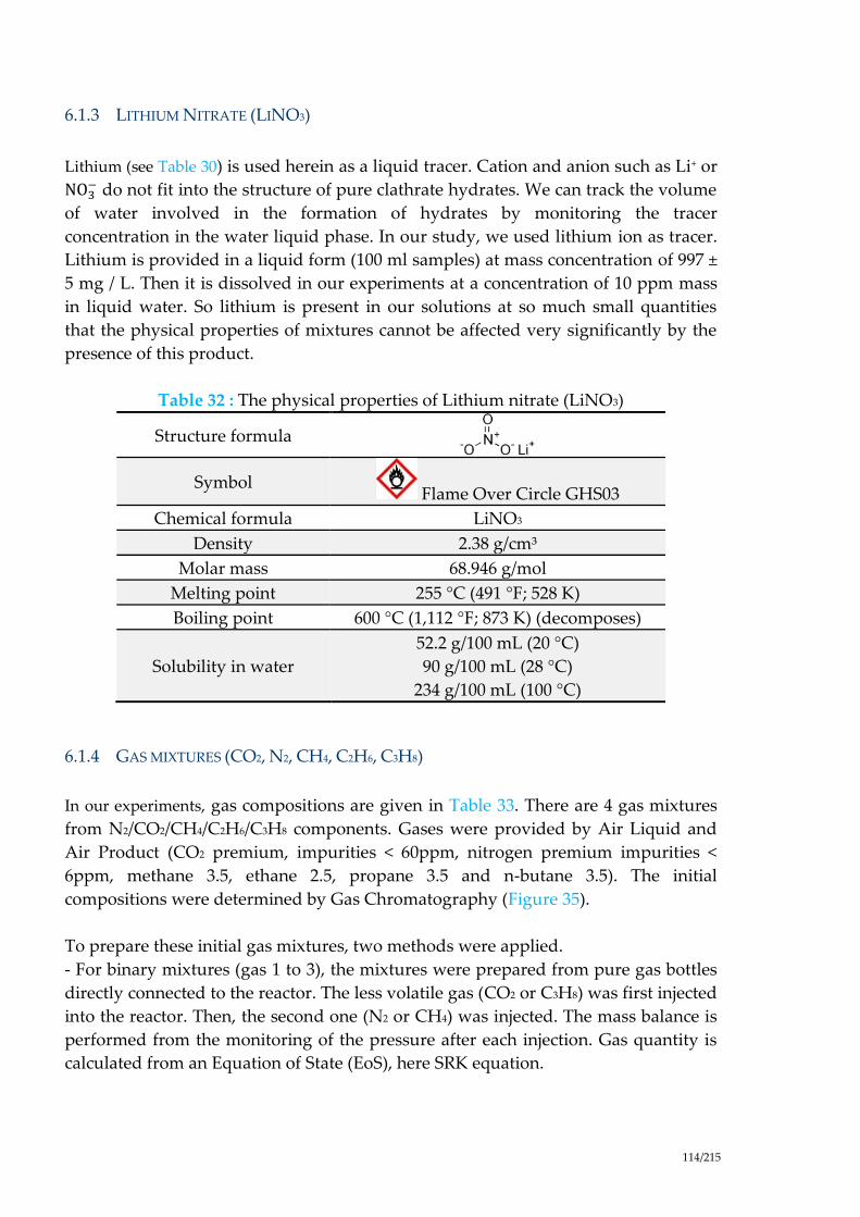
114/215

6.1.3 LITHIUM NITRATE (LINO3)

Lithium (see Table 30) is used herein as a liquid tracer. Cation and anion such as Li+ or

NO3− do not fit into the structure of pure clathrate hydrates. We can track the volume

of water involved in the formation of hydrates by monitoring the tracer

concentration in the water liquid phase. In our study, we used lithium ion as tracer.

Lithium is provided in a liquid form (100 ml samples) at mass concentration of 997 ±

5 mg / L. Then it is dissolved in our experiments at a concentration of 10 ppm mass

in liquid water. So lithium is present in our solutions at so much small quantities

that the physical properties of mixtures cannot be affected very significantly by the

presence of this product.

Table 32 : The physical properties of Lithium nitrate (LiNO3)

Structure formula

Symbol Flame Over Circle GHS03

Chemical formula LiNO3

Density 2.38 g/cm³

Molar mass 68.946 g/mol

Melting point 255 °C (491 °F; 528 K)

Boiling point 600 °C (1,112 °F; 873 K) (decomposes)

Solubility in water

52.2 g/100 mL (20 °C)

90 g/100 mL (28 °C)

234 g/100 mL (100 °C)

6.1.4 GAS MIXTURES (CO2, N2, CH4, C2H6, C3H8)

In our experiments, gas compositions are given in Table 33. There are 4 gas mixtures

from N2/CO2/CH4/C2H6/C3H8 components. Gases were provided by Air Liquid and

Air Product (CO2 premium, impurities < 60ppm, nitrogen premium impurities <

6ppm, methane 3.5, ethane 2.5, propane 3.5 and n-butane 3.5). The initial

compositions were determined by Gas Chromatography (Figure 35).

To prepare these initial gas mixtures, two methods were applied.

- For binary mixtures (gas 1 to 3), the mixtures were prepared from pure gas bottles

directly connected to the reactor. The less volatile gas (CO2 or C3H8) was first injected

into the reactor. Then, the second one (N2 or CH4) was injected. The mass balance is

performed from the monitoring of the pressure after each injection. Gas quantity is

calculated from an Equation of State (EoS), here SRK equation.

https://en.wikipedia.org/wiki/Chemical_formula

https://en.wikipedia.org/wiki/Density

https://en.wikipedia.org/wiki/Molar_mass

https://en.wikipedia.org/wiki/Melting_point

https://en.wikipedia.org/wiki/Boiling_point

https://en.wikipedia.org/wiki/Aqueous_solution

115/215

- The second method was to connect a former prepared bottle. This bottle was

prepared by injecting the different gases, from the less volatile to the most volatile,

and weighting the bottle after each injection. In order to have a quite homogeneous

mixture, the bottle is not used before a few days after the preparation. The maximum

pressure is 20% less than the gas mixture dew point to be sure avoiding any

condensation.

Table 33: Molar composition of the experiments gas mixtures (standard deviation

about 3%)

Gas

mixtures

CO2

(%)

N2

(%)

CH4

(%)

C2H6

(%)

C3H8

(%)

n-C4H10

(%)

Gas 1 0.821 0.179 -- -- -- --

Gas 2 0.053 -- 0.919 0.028 --

Gas 3 -- -- 0.846 -- 0.154 --

Gas 4 -- -- 0.950 0.029 0.021 --

6.2. EXPERIMENTAL DEVICE

The reactor is a cylindrical glass vessel with diameter and height of 108 mm and 175

mm, respectively. The volume is 2.44L (ACACIA system) or 2.36L (SECOHYA

system). The cylindrical glass vessel is filled in our experiments with a liquid water

(deionized water plus Lithium) of 800-1100 ml volume, which corresponds to a

height of liquid is 87-120 mm. The vessel is enclosed in an autoclave provided with

two windows allowing a direct observation. The portholes (12cm x 2cm) allow us to

check formation or dissociation of hydrates, but also to observe qualitatively the

behavior, and to observe if particles are floating, or sticking at surfaces such as the

stirrer. It allowed us to see that the liquid sampler is a free zone without particles.

116/215

Figure 33: Experimental set-up

The autoclave is surrounded by a cooling jacket and cooled or heated by a cryostat

(HUBERT CC-505) which temperature control is 0.020C accuracy. The circulating

refrigerant mixture consists in a mixture of water and ethanol (96% vol.) circulating

into a cooling jacket. From a practical point of view, to take into account thermal

losses, the cooling liquid is controlled at a temperature of 1 to 2 °C lower than the

operative temperature inside the reactor.

The stirrer is a two blades impeller of 71.4 mm diameter and 10.2 mm height. It is

positioned at a distance of about 25 mm from the bottom of the reactor. The stirrer is

magnetically driven from 0 to 600 rpm (rotation per minute). The measurement of

the stirring rate is directly done using a portable optical tachometer (Lutron DT-

2236).

A JASCO PU-1587 high pressure pump can inject the liquid inside the pressurized

reactor, at a rate upt to 15 ml/min. The injection of the liquid is performed after the

gas input.

The temperature sensor is a Pt100 probe that is immerged in the liquid reaction

medium, before crystallization, and in the slurry medium during crystallization. It is

linked to a WEST (8010) electronic device which converts the voltage signal into

temperature, expressed in degrees Celsius. The pressure is also measured by a

pressure sensor in the range 0-10 MPa. The pressure sensor is also connected to a

117/215

WEST (8010) device. The accuracy of the sensor is estimated at 0.4% over the entire

pressure range. These two acquisition systems are connected to a computer and a

program monitoring in LabVIEW language.

A ROLSI® (Rapid On-line Sampler-Injector) manufactured by the Paris School of

Mines (Laboratory CEP/TEP) is attached to the top of the autoclave and allows gas

sampling (Baba-Ahmed et al., 1999; Guilbot et al., 2000). It consists of a capillary tube

of 0.1 mm inner diameter opening on one side in the gaseous headspace of the

reactor and on the other side into a chamber through which is circulated the carrier

gas to the Gas Chromatography. The side of the capillary connected to the sampler

body is sealed by a mobile part whose upper and lower extremities consist of,

respectively, a polymer part and a soft iron core, the latter being constrained by a

spring. Samples are withdrawn by the action of an electromagnet which attracts the

mobile part and opens the seal between the fixed capillary and the mobile part. The

pressure inside the cell is higher than that in chromatographic circuit and, therefore,

the sample flows through the stem of the sampling valve. After the sampling valve is

closed, the sample is taken out by the carrier gas up to gas chromatograph. The

amount of the withdrawn sample depends on pressure and temperature conditions

and it is directly proportional to the seal opening time. This quantity obviously

depends on the conditions of temperature and pressure, but the volume is of the

order of 1- 5 𝜇l, which is negligible in comparison to the free volume of the gas that

is about 1L. A heating system incorporated into the body of the ROLSI can avoid, if

necessary, the condensation of the gas. This sampling system coupled to a

chromatograph is a complete in-situ analysis of the gas phase system.

Figure 34: Schematic of Electromagnetic version of the ROLSITM Sampler injector.

A: carrier gas inlet; B: capillary; C: body; D: carrier gas outlet; E: moving part set in

motion by the electromagnet; F: electromagnet; G: return spring; H: power supply

coupled with a timer; I: soft iron core; J: cooling fins.

118/215

The gas samples of gas phase were analyzed by using a VARIAN chromatograph

(Model 3800 GC) equipped with a TCD detector in Figure 35. Chromatographic

analysis is based on the principle of affinity of a solute between a moving phase

(carrier gas) and a stationary phase contained in a thin and long tube. There are two

types of columns depending on the nature of the stationary phase therein. We

distinguish packed columns and capillary columns. The columns filled are usually

made of metal, with a diameter of several millimeters and filled with a porous

granule. The capillary columns are empty tubes, usually silica, where the stationary

phase is deposited on the inner wall in the form of an as regular as possible film.

Their diameter is less than packed columns. The injection of gas samples to the head

column is realized through the ROLSI system, and pushed through the column by a

carrier gas. They are going to be separated from one to another when passing

through of the column according to their affinity with the stationary phase. The time

taken to run through the column and reach the detector is the retention time. There

are principally two types of detector: TCD (Thermal Conductivity Detector) and FID

(Flame Ionization Detector). The principle of the TCD is based on the measurement

of the thermal conductivity of the gas mixtures. An acquisition and data processing

system is connected to the chromatographic system.

Figure 35: Schematic of the VARIAN chromatograph (Model 3800 GC) equipped

with a TCD detector.

In our applications a double column system was specifically designed. It is two

columns in parallel (PoraBOND Q and a CP-Molsieve 5A columns) for the detection

and separation of a wide range of gas. PoraBOND Q is a column filled or packed

with an inner diameter of 0.53 mm and a length of 50 m. It is capable of eluting

compounds such as alcohols, hydrocarbons (C1-C9), H2S, CO2 and other solvents.

Molsieve 5A is a capillary column with an internal diameter of 0.32 mm and a length

of 10 m. It is capable of holding permanent gases such as H2, N2, Neon, Ar, Krypton,

O2, CH4, CO. Methane is retained in the two columns. It can therefore be used to

119/215

determine the sample sharing ratio between the two columns. An illustrative

diagram of the chromatographic system is proposed in Figure 45. Please note that

the injector is the output of ROLSI Figure 34.

The sampling system of the liquid phase consists of a tube 1/16 inch immersed in the

liquid and connected to a valve. The position of the tube depends on the density of

the hydrates formed. If they are lighter than the liquid, they float and the tube is then

positioned toward the bottom of the reactor at a distance approximately equal to 30

mm, that is to say practically the same level as the stirrer blades. We have noticed

that gas hydrates such as CO2 and N2 hydrates, or hydrates formed from the mixture

of these two gases are floating. So it is for CH4 and C3H8.

The lithium concentration in the liquid is determined by Ionic Chromatography (IC)

in Figure 36. The principle is substantially the same as in the gas chromatography.

The fundamental difference is the nature of the mobile and stationary phases. In the

case of detection of lithium (Li+, a cation), the stationary phase is a polymer with

attached anionic groups (sulfonate). The eluent or mobile phase is methane sulfonic

acid (HMSA). In our application, we have a DX50 chromatograph equipped with a

Dionex Company CS12A column and a TCD detector. The signal obtained at the

detector output is processed by a computer.

Figure 36: The system of the ionic chromatography at SPIN laboratory

120/215

6.3. EXPERIMENTAL PROCEDURE

6.3.1 HIGH CRYSTALLIZATION RATE

The first experimental procedure is the same as in our previous studies on gas

hydrates equilibrium (Herri et al., 2011). In this procedure, the crystallization occurs

at a “high rate” (or at a high supersaturation). At first, the reactor is cleaned and

vacuumed (for 40-50 minutes). Then, the cell is filled with the operative gas

composition either by direct injection of the various components, or from a bottle

where the mixture has been prepared before.

The pressure is measured, and the temperature is set to 1°C (internal regulation of

the cryostat). The gas composition in the cell is checked with GC analysis before any

measurement.

A 10 mg/L water mixture of LiNO3 is prepared and injected (about 800-1000g) into

the reactor thanks to the HPLC pump (n°08 on Figure 33). The water is ultrapure

water (first category, 18.2 MΩ.cm). A raise of the pressure, due to the added volume

of liquid, is observed. Then, the reactor is stirred at the rate of 450 rpm, on the gas

upper side, and on the liquid bottom side. The gas is dissolving into the liquid

phase, and after some time (induction time), the crystallization begins. Due to the

exothermicity of the reaction, a brief raise of temperature is observed. At this point,

we wait for the equilibrium (no more temperature and pressure time evolution). This

takes about 2 to 4 days depending on the mixture and initial pressure. As the

equilibrium is reached, a sample of the gas phase is taken and injected into the gas

chromatograph to determine the molar composition. A liquid sample is also taken to

be analyzed offline by ionic chromatography (about 4.5-5.5mg). Then, the

dissociation of the hydrate is started. The temperature is increased of about 1-2°C.

When the new equilibrium is reached (after 24h), new samples of the fluid phases

are taken. Then, the process is repeated until there is no longer a hydrate phase into

the reactor. The whole procedure is summarized on Figure 37 and Figure 38.

121/215

Figure 37: The procedure of the high crystallization rate

Figure 38: P– T evolution during equilibria experiments at high crystallization rate.

6.3.2 LOW CRYSTALLIZATION RATE

In this second procedure on Figure 39, the objective is to focus on thermodynamic

equilibrium avoiding as much as possible any kinetic effect. The objective is to stay

as close as possible to the thermodynamic equilibrium curve, in order to decrease

kinetic effects on crystallization.

122/215

The pressure/temperature evolution in function of the time is shown on Figure 40.

Instead of decreasing very quickly the temperature to the final point (between 0 and

2°C), the crystallization occurs close to the initial point in the hydrate free area. Then,

the temperature is decreased very slowly (about 0.1- 0.3 °C per day). Each 1°C step,

samples of the gas and liquid phases are taken and analyzed in Gas Chromatograph

and Ionic Chromatography, respectively. This procedure concerns only gas mixture

n°2, 3 and 4 on Table 33.

Figure 39: The procedure of the low crystallization rate.

Figure 40: P – T evolution during equilibrium experiment at low crystallization rate.

123/215

6.4. OPERATING PROTOCOLS

6.4.1 DETERMINATION OF THE CONCENTRATION OF LITHIUM BY IONIC

CHROMATOGRAPHY.

The determination of lithium ion concentration (Li+) is carried out by Ionic

Chromatography in Figure 36. The column was at ambient temperature and the

TCD detector is thermostatic. The analysis protocol consists in diluting the sample

by a factor in between 2 and 10, with a very high precision micropipette. This

dilution is necessary because the sample to be analyzed should be 5 ml minimum

whereas the volume recovered is around the value of 2 ml. In fact we need to

minimize the sampling volume to avoid distorting the mass balance on the liquid.

After dilution, the sample is passed through the chromatographic system, which

output gives a chromatogram with peaks. This chromatogram is integrated through

a computer that provides the peak areas.

Figure 41 is given an example of a chromatogram of a sample from the reactor. The

peak corresponding to Li+ ions is at retention time of 3.847 min and shows a good

resolution. The peak corresponding to sodium is probably due to some remaining

traces from a previous analysis of a solution containing sodium. The peak with a

negative intensity corresponds to an artifact of measurement.

Figure 41: Chromatogram of a liquid sample - Analysis of Lithium

The establishment of a calibration curve is done at each series of measurements. This

is explained by the fact that ambient conditions change, but also the concentration of

the mobile phase is not be always the same. A conventional calibration method is

possible. The principle of this method is to establish a simple relationship between

the concentration of Li+ and the peak area obtained by injecting standard solutions of

known concentrations.

124/215

Figure 42: Calibration curve of the ionic chromatography

Figure 42 is showed the right chromatograph calibration for a series of

measurements. On the abscissa we have Li+ ion concentration in ppm and the

ordinate the peak area. We can see that the linearity relationship is well respected in

the range [0-20 ppm], corresponding to our samples taken from the reactor, or after

dilution.

6.4.2 CALIBRATING THE GAS CHROMATOGRAPH (TCD)

A gas chromatograph (GC) is an analytical instrument that measures the content of

various components in a sample. The analysis performed by a gas chromatograph is

called gas chromatography. The gas chromatograph allows us to know the

composition of a gas mixture. Indeed, the area of a peak given by the chromatogram

is proportional to the amount of material in the sample.

Based on the laboratory experience and on the existing laboratory equipment the gas

chromatography method was selected to perform the analyses. The Gas

Chromatograph used is the Varian 3800 GC model on Figure 35. The

chromatographic technique allows separating and quantifying the products a

sample.

Figure 43: GC principle

Injector Column Detector

Carrier Gas Acquisition

125/215

The separation and the quality of the analysis is a function of the following

parameters:

- Choice of the column,

- Temperature/Pressure of the oven column,

- Choice of the carrier gas,

- Flow rate of the carrier gas,

- Parameters of the detectors.

The chosen carrier gas, which has been used for most of the study, is helium (except

for a set of test, where the carrier gas was nitrogen). To obtain a maximum

sensitivity of the detector (thin peaks) the carrier gas flow rate is adjusted. Helium

from Air Liquide (or Air Product) is pure grade with 3 ppm water trace and 0.5 ppm

hydrocarbon traces (see at Table 31). To purify the carrier gas, the gas is cleaned by a

molecular sieve, positioned at the outlet of the helium bottle.

Two detectors are used to perform the analyses: a Thermal Conductivity Detector

(TCD) and a Flame Ionization Detector (FID), connected in series.

The TCD measures continuously the variation of the thermal conductivity of the

carrier gas. The TCD is non-destructive detector. To achieve a good analysis of the

samples, the thermal conductivity of each compound must be as different as possible

of that of the carrier gas (see Table 31).

The FID is detector, which measures the compound capabilities to form ions when it

goes through the flame. The FID is a destructive detector, thus it is connected in

series, at the outlet of the TCD.

The operating conditions of the chromatograph were optimized to shorten the

analysis time but also to get a good resolution and separation of peaks. For this we

mainly adjusted the oven temperature, the pressure and the carrier gas flow. We

must remember that these variables play a first order role in the compound retention

time in the column. Oven Temperature, and most important carrier flow, tends to

reduce the retention time but in return a less clear separation of certain compounds.

A compromise is to find. At an oven temperature of 40°C and a carrier gas flow of

2.7 ml/min, elution of CO2 is 22 min. This retention time is too much important to

follow the crystallization kinetics. We increased the oven temperature to 50°C (up to

180°C) and increased the carrier gas flow between 15 and 50ml/min. the pressure

was chosen 23 psi. With these conditions shown in Table 34, we can analyze a

sample of gas mixture in less than 7-8 minutes with distinct peaks. The quality of the

separation is not affected.

126/215

We chose in our analysis to check the reproducibility of results by injecting the same

sample twice with an interval of 2 minutes between the first and second injection.

Table 34 : Operating conditions of the chromatogram

Injector temperature, oC 200

Detector temperature, oC 220

Filament temperature, oC 270

Oven temperature, oC 50-180

Carrier gas Helium (He)

Carrier gas pressure, psi 14 or 23

Carrier gas flow rate, ml/min 15-50

In chromatography, for a binary gas mixtures A+B of quantity 𝑚𝑇, the area of a peak

is in general proportional to the amount of injected material 𝑚𝑇. For a compound

(A), peak area (S) that by:

𝑆𝐴 = 𝐾𝐴𝑚𝐴 = 𝐾𝐴𝑚𝑇𝑥𝐴 (109)

Where 𝑥𝐴is the molar fraction of component A and 𝑚𝑇 the mass of all the species. In

the classical method of the calibration the proportionality constant 𝑘𝐴 would be

determined by injecting a sample even if the amount of A is known. In our sample

system, we can not ensure that we take the same amount of gas that the conditions

of pressure and temperature change from one experience to another:

𝑚𝑇 =

𝑃𝑉

𝑍𝑅𝑇𝑀𝑇 (110)

Where 𝑀𝑇 the molar mass of the gas mixtures and Z is the compressibility factor and

V is the volume.

We have also chosen to perform relative calibration in using the report of the

compositions of a binary gas mixture is analyzed. Finally, the results are

independent of initial quantities injected:

ATAAAA xnknkS (111)

B

A

B

A

B

A

B

A

x

xk

x

x

k

k

S

S (112)

BTBBBB xnknkS (113)

127/215

But, in our experiment, the amount of component cannot be determined after

sampling due to the method itself. In fact, the ROLSI instrument is a valve that is

opened during a period of time. During this period, the amount of material is

proportional to the flow rate, and the flow rate is directly proportional to the

pressure. The pressure is not a controled parameter, but is dependent from

equilibrium considerations, or time consideration is the equilibrium is not reached.

The principle of the preparation of the gases is to generate a binary mixture (for

example gas A and gas B) with a given mole fraction composition 𝑥𝐴 and 𝑥𝐵

respectively, and to compare the ratio (𝑆𝐴

𝑆𝐵) of the surface of the respective

chromatograph peak. Once the gas composition is determined, a gas

chromatography is performed, and the respective surface areas ratio of gas A and B

(𝑆𝐴

𝑆𝐵) is measured and correlated to ratio of respective gas composition (

𝑥𝐴

𝑥𝐵).

The peak surface area is estimated with an error S/S = 0.05.

The result is a calibration curve (Figure 44) which gives estimation of (𝑥𝐴

𝑥𝐵) plus or

minus 1%.

Figure 44: Calibration curve of gas chromatograph

For a new sample, the chromatographic analysis allows obtaining the peak areas

relative to each compound. To know the composition of the sample, the following

system of equations is used.

{

𝑥𝐴

𝑥𝐵= 𝑎

𝑆𝐴

𝑆𝐵+ 𝑏

𝑥𝐴 + 𝑥𝐵 = 1

(114)

𝑥𝐴

𝑥𝐵

𝑆𝐴

𝑆𝐵

128/215

For instances, the calibrations were performed for the A+B gas mixtures. The

operating procedure is as bellows:

Initially, the system is emptied by the using vacuum pump installed on the

circuit is maintained at approximately 279 oK constant temperature by using

the cryostat consigned to 278 oK.

The reactor charged with (A) molecules reaches a certain pressure P1. Once

the pressure and temperature is stabilized, a gas sampling is performed to

verify that the reactor is only filled with gas (A).

The second gas (B) is subsequently introduced into up to pressure P2.

The gas mixture in the reactor is stirred at ~400 rpm. When the pressure and

temperature are stabilized in the reactor, the mixture was analyzed by gas

chromatography (GC).

Analysis of the mixture takes place as follows: At first, we purge 10 times the

system by pushing the button and opening the Rolsi valve during 0.01s each

time. It ensures withdrawing the gas mixtures from the rolsi instrument itself.

After waiting 150 seconds, the test sample is injected into the gas

chromatograph flow line from a new push on the button to open it during

0.01s. GC analysis takes about 7-9 minutes. Each analysis is done twice to

ensure reproducibility of the results. In the end, it takes 20 minutes for a

complete analysis.

This calibration can be done from a prepared gas mixture (see section §6.1.4, Page.

114). In this case, we have to wait a few days for the homogeneity of the gas mixture.

This calibration method compares the areas of the peaks. The different gases used

are retained in both the two columns of the chromatograph. Therefore, there is a

choice in the peak to exploit. For the three gases, we chose to exploit the second

peak, from the Q PoraBOND column that are better than those from the Molsieve 5A

column. As an example, Figure 45 shows the peaks for CO2-N2 mixture. Usually, the

major molecule is used as reference since it is the peal wit the best accuracy (CH4 as

example).

129/215

Figure 45: Chromatogram of a sample of CO2-N2 mixtures

6.4.3 MASS BALANCE CALCULATION

At any moment, the initial quantity of the gas molecules is distributed between

all the phases: gas phase, liquid phase and solid hydrate phase. Thus, in equilibrium,

the quantity of gas in the hydrate phase can be determined from a mass balance

according to:

𝑛𝑖,0𝑖𝑛𝑖𝑡𝑖𝑎𝑙 = 𝑛𝑖

𝐺 + 𝑛𝑖𝐿 + 𝑛𝑖

𝐻 (115)

Where 𝑛𝑖,0𝑖𝑛𝑖𝑡𝑖𝑎𝑙 is the mole number of the gases injected inside reactor, and

𝑛𝑖𝐺 , 𝑛𝑖

𝐿 , 𝑛𝑖𝐻 are the mole numbers of the gaseous component i (i: CO2, N2,

hydrocarbon) in the hydrate, the liquid and the gas phase, respectively. We will only

consider an aqueous phase for the liquid phase.

The amount of substance of the gases dissolved in the liquid phase is then

estimated by means of corresponding gas solubility data into water, whereas the

mole number of the gases present in the gas phase is calculated by using an equation

of state approach as outlined in the next sections.

• Calculation of compressibility factor

The compressibility factor in the gas phase in any equilibrium state can be

calculated by means of the classical Eq. (116) combined with a suitable equation of

state (EOS), e.g., a classical cubic EOS. For this study, the Soave-Redlich and Kwong

(SRK) EOS has been used with parameters from (Danesh, 1998) given in Table 35.

𝑍(𝑇, 𝑃,�⃗�) =

𝑃𝑉

𝑛𝑅𝑇 (116)

130/215

with Gnn (at each situation) and T, P, V are the temperature, pressure and phase

volume, �⃗� = (𝑥1, … 𝑥𝑛), represents the vector of the mole fractions of the components

in the mixture, 𝑛 the total mole number in the gas mixture, and 𝑅 the universal gas

constant.

Table 35: SRK parameters

j Tc(K) Pc(bar) ω k(N2/j) k(CO2/j) k(CH4/j) k(C2H6/j) k(C3H8/j) k(n-

C4H10/j)

N2 126.20 34.00 0.03772 0 -0.03 0.03 0.06 0.09 0.1130

CO2 304.21 73.83 0.22362 -0.03 0 0,0933 0,1363 0,1289 0,1430

CH4 190.56 45.99 0.01155 0.03 0,0933 0 -0,0078 0,009 0,0056

C2H6 305.32 48.72 0.09949 0.06 0,1363 -0,0078 0 -0,0022 0,067

C3H8 369.83 42.48 0.15229 0.09 0,1289 0,009 -0,0022 0 -0,01

n-C4H10 425.15 37.99 0.2013 0.1130 0,1430 0,0056 0,067 -0,01 0

• Composition of the gases initial inside reactor

Before injecting water inside reactor, the mole fraction of each gas in the gas phase xj

is determined by using gas chromatography analysis.

We recall here that the reactor of total inner volume VR = 2.44L (ACACIA system) or

2.36L (SECOHYA system) is initially filled with the gaseous components at the

initial temperature 0T and pressure 0P .

𝑛0

𝐺 =𝑃0𝑉𝑅

𝑍൫𝑇, 𝑝, 𝑦𝑗,0൯𝑅𝑇0

(117)

GC analysis provides the gas phase composition only. Each component j has an

initial mole fraction xji (j is CO2, N2, hydrocarbons). Combined with the

measurements of temperature, pressure, and compressibility factor in the gas phase,

the initial total mole number in the gas phase G

0n is derived from Eq. (117). We also

obtaine the mole number of each gas

• Volume of the aqueous phase:

As mentioned before, the liquid phase contains LiNO3 as a tracer. Initially the

concentration of lithium 0]Li[ and the initial volume of liquid L

0V are known.

During the crystallization and dissociation steps, the concentration of lithium is

measured by ion-exchange chromatography after sampling. So, we can calculate the

volume of liquid water from a mass balance for the Li+ ions:

131/215

𝑉0

𝐿[Li+]0 = 𝑉𝐿[Li+] ⇒ 𝑉𝐿 =𝑉0

𝐿[Li+]0

[Li+] (118)

Where LV and [Li+] are the volume of the liquid aqueous phase and the molar

concentration of lithium in this phase, i.e. in the sample, corresponding to a given

step of the crystallization or dissociation.

• Water mole number in the hydrate phase

The quantity of water molecules involved in the hydrate structure can be calculated

from:

L

0 wL

w

L

w

V Vn

M

(119)

L

w

L VV stands for the volume of the liquid phase in equilibrium, w the liquid

water density (about 1kg/L at 4oC), and wM is the molar mass of pure water

(18g/mole).

• Mole fraction of the solubility of gases in liquid phase

The solubility of a gas in a liquid is determined by the equations of phase

equilibrium. If a gaseous phase and a liquid phase are at equilibrium, then for any

component i the fugacity in both phases must be the same:

𝑓𝑖𝐿 = 𝑓𝑖

𝑉 (120)

The symmetric approach, called (∅𝑣 = ∅𝐿), consists in describing the gas

phase and the liquid phase in terms of equations of state (EOS) along with

appropriate mixing rules

∅𝑖𝑣𝛾𝑖

𝑣 = ∅𝑖𝐿𝑥𝑖

𝐿 (121)

The classical or unsymmetrical approach, called , consists of choosing an

equation of state (EOS) for the gas phase and a excess model for the liquid

phase:

∅𝑖𝑣𝑦𝑖

𝑣𝑃 = 𝛾𝑖𝑥𝑖𝑓𝑖0𝐿 (122)

132/215

𝑓𝑖0 is the reference state and can be either the pure liquid or the infinitely

diluted compound (Henry’s law). In the case of pure liquid, L

if0 is expressed as

function of the saturated vapor pressure of the liquid

𝑓𝑖

0𝐿 = 𝑃𝑖𝑠𝑎𝑡∅𝑖

0(𝑇, 𝑃𝑖𝑠𝑎𝑡)𝑒𝑥𝑝 (

𝑣𝑖൫𝑃−𝑃𝑖

𝑠𝑎𝑡൯𝐿

𝑅𝑇) (123)

L

iv is the molar volume of the pure liquid component i (i = solvent) at

saturation. The exponential term is called Poynting correction factor. It

represents the deviation between the saturated vapor pressure of component i

and the equilibrium pressure.

For treating the gas solubility in our system, the unsymmetrical approach is used

and combined with the unsymmetrical convention (Henry’s law approach), which

corresponds to infinite dilution reference (i.e. the activity coefficients of the gas

molecules into the water equal to unity). The equilibrium condition reads:

∅𝑖𝑣𝑦𝑖

𝑣𝑃 = 𝛾𝑖𝑥𝑖𝐻𝑖 (124)

where Hi is Henry’s law constant. It is expressed by means of the following relation:

𝐻𝑖 = 𝐻𝑖,𝑃𝑠𝑎𝑡𝑒𝑥𝑝 (

𝑣𝑖∞(𝑃 − 𝑃𝑖

𝑠𝑎𝑡)

𝑅𝑇) (125)

The so-called solubility models enable the calculation of Henry’s law constant. It has

to be reminded that the Henry’s law constant is determined at the saturated vapour

pressure of the pure solvent ( PsatiH , ). Thus, the Poynting factor corrects for the

pressure difference between Psat of the pure solvent (here is the water) and the

system pressure P. The partial molar volume of the gas i at infinite dilution (

i ) can

be calculated from a correlation proposed by (Vidal et al., 1973a, 1973b). However, it

is fixed here to 32 cm3 .mol-1 for the majority of the components.

(Holder et al., 1980; Holder and Grigoriou, 1980) proposed the following correlation

for Henry’s constant at saturation with temperature:

𝐻𝑖,𝑃𝑠𝑎𝑡 = 𝑒𝑥𝑝 ൬𝐴 +

𝐵

𝑇൰ (126)

The coefficients A and B are compiled in Table 36. The temperature is expressed in

Kelvins and Henry’s constant is given in atmospheres.

133/215

Table 36: Constants for calculating Henry’s constant (Holder et al., 1980)

• Mole number of gases in the liquid phase:

From Eq. (124), and Eq. (125), the expression for the mole number L

in of the gas i

dissolved in the liquid phase:

LL w

w , exp

v

i ii

i Psat i

V y Pn

M H Pv RT

(127)

L

w

L VV stands for the volume of the liquid phase in equilibrium, w is the density,

and wM is the molar mass of pure water. 13 molcm32 jv is (an average value from

Holder in Table 36) the partial molar volume of the gas i in the solvent water. In

establishing Eq. (127), the activity coefficient of gas in water was in a good

approximation neglected and the very good approximations L

w

L nn j , and L

w

L VV

were applied.

• Composition of the gases in gas phase

Eq. (117) has also been used to determine the total amount of substance of the gas

phase in a state corresponding to the three phase hydrate-liquid-vapor equilibrium.

In the latter case, the initial values of the variables are to be replaced by the

corresponding values measured in that equilibrium state, i.e, 0T , 0P , 0,jy and G

0n are

to be substituted for T, P, jy and Gn . The volume of the reactor VR has been replaced

by the actual value of the gas phase GV , which for any given equilibrium state has

been approximated by:

G

R w, 0 sampleV V V V (128)

Gas A B

i (Cm3/mole)

CH4 15.826277 -1559.0631 32

C2H6 18.400368 -2410.4807 32

C3H8 20.958631 -3109.3918 32

n-C4H10 22.150557 -3407.2181 32

CO2 14.283146 -2050.3269 32

N2 17.934347 -1933.381 32

134/215

Where 0,wV stands for the volume of the liquid water, the reactor is initially loaded

with. sampleVis the volume of the liquid sampled for ionic chromatography.

Utilizing the results from the gas chromatographic analysis we got mole fraction of

each gas in composition ( ix ). Combining GV and ( ix , P, T) we can be calculated G

in

by means of a suitable equation of state (EOS), here the Soave-Redlich and Kwong

(SRK).

• Composition of hydrate phase

The hydrate phase calculation comes from a mass balance Eq. (115). The hydration

number is also obtained from the quantity of water consumed by the cristallization

and also calculated from Eq. (129).

𝑛𝐻𝐷𝑌 =𝑚𝐻𝑦𝑑𝑟𝑎𝑡𝑒

𝑀𝐻2𝑂 ∑ 𝑛𝐻𝑦𝑑𝑟𝑎𝑡𝑒 (129)

• A few words about experimental errors

Evaluation of errors of the calculations was made and written previously (Galfré,

2014; Herri et al., 2011). This last evaluation led to an uncertainty on the gas phase

equals to x/x < 3% (determined from GC errors), and to an uncertainty of the

hydrate phase of z/z < 6% (See Appendix 3 is presented in section §14. Page. 209).

In the present work, another evaluation was performed using Monte Carlo

simulations.

Monte Carlo method for evaluating the uncertainties consists in performing a huge

number of calculations by taking into account the uncertainties of the inputs. It is

usual to consider that the uncertainties follow a Gaussian law. Hence, they are

represented by their mean values and standard deviation. A significant number of

calculations are then done (about 1000 simulations). Each time, new random values

for the inputs are used according to Gaussian law.

In the end, there are as many different outputs as there are simulations. A quick

statistical evaluation leads to the mean results (hydrate volume, composition…), and

their standard deviations.

To compute each time these 1000 simulations, the following standard deviations of

the input data were used:

135/215

- [Li+]/[Li+] = 0.1%,

- xi/xi = 3%,

- T = 0.2°C,

- P = 0.1 bar,

- mw = 0.1g,

- mw (sampled) = 0.1g,

- VR = 3%,

- ρw = 10 kg.m-3,

- ρHβ = 40 kg.m-3.

Also, the following assumptions were done:

- Ρw = 1000 kg/m3.

- ρHβ = 790 kg/m3.

We observed that the molar fraction errors on the hydrate composition were found

to be usually inferior to 4%. The standard deviation close to the total dissociation

point was calculated to be between 20% and 100%. Indeed, the initial and final Li+

concentrations for these points are very close.

136/215

137/215

7. EXPERIMENTALS RESULTS AND DISCUSSIONS

Experimental gas compositions are presented in Table 37. Here are presented

experimental results from both procedures (quick and slow crystallization). Each of

them are applied to measure the composition of the hydrate formed from different

gas mixtures from CO2-N2-CH4-C2H6-C3H8 … Corresponding PT results (Pressure

and Temperature) are observed carefully in order to investigate the influence of the

crystallization rate on the hydrate formation. In a second approach, these results are

compared to a thermodynamic modelling (when it is possible). The objective of these

simulations is to check the assumption that quick crystallization leads to kinetic

equilibria. The simulated results are obtained from our in-house program

GasHyDyn.

Table 37: Molar composition of the studied gas mixtures and initial conditions of

experiments.

Gas

mixtures

(Exp)

Methods

CO2 N2 CH4 C2H6 C3H8 Pi Ti Reactor

volume

Mass

water

injected

%

(±0.001)

%

(±0.001)

%

(±0.001)

%

(±0.001)

%

(±0.001)

MPa

(±0.001)

oK

(±0.2)

Lite

(±0.001)

Gram

(±0.1g)

Gas 1 Quick 82.08 17.92 -- -- -- 3.11 278.2 2.44 800.9

Gas 2 Quick 82.81 17.19 -- -- -- 3.13 277.9 2.44 800.9

Gas 3 Quick 0.057 -- 0.915 0.028 -- 3.25 275.8 2.36 801.3

Gas 4 Quick 0.053 -- 0.919 0.028 -- 2.20 278.0 2.36 799.6

Gas 5 Slow 0.052 -- 0.919 0.029 -- 4.73 276.4 2.36 800.3

Gas 6 Slow -- -- 84.61 -- 15.39 1.73 280.0 2.36 801.1

Gas 7 Slow -- -- 84.61 -- 15.39 1.73 280.0 2.36 801.1

Gas 8 Slow -- -- 86.86 -- 13.14 1.83 285.0 2.36 800.9

Gas 9 Quick -- -- 85.77 -- 14.23 1.81 281.0 2.36 801.2

Gas 10 Quick -- -- 85.81 -- 14.19 1.71 280.5 2.36 801.1

Gas 11 Quick -- -- 86.89 -- 13.11 1.77 285.1 2.44 800.9

Gas 12 Quick -- -- 86.89 -- 13.11 1.77 285.1 2.44 800.9

Gas 13 Slow -- -- 95.02 2.90 02.08 2.78 285.1 2.36 801.1

Gas 14 Slow -- -- 87.72 -- 12.28 1.81 284.8 2.36 801.4

Gas 15 Quick -- -- 87.72 -- 12.28 1.81 284.8 2.36 778.0

Gas 16 Quick -- -- 86.37 -- 13.63 1.78 284.1 2.36 801.4

Gas 17 Slow -- -- 86.37 -- 13.63 1.78 284.1 2.36 801.4

In the next sections, tables Table 38, Table 39 and Table 40 present the simulated

results (predicted pressures and hydrate compositions) and the mean deviations to

experimental results.

138/215

7.1. CO2-N2 GAS MIXTURES

Table 38: CH_SI-V-Lw Equilibrium of CO2-N2 at quick crystallization rate procedure

versus predicted results


T

(±0.2)

P

(±0.01)

Gas composition Hydrate

composition

S P

Hydrate

composition

Molar gas fraction (±0.001) Molar gas

fraction (±0.003)

CO2 N2 CO2 N2 CO2 N2

(°C) (MPa) (%) (%) (%) (%) MPa (%) (%)

2.3 2.46 0.667 0.333 0.970 0.030 SI 2.53 0.955 0.045

3.1 2.60 0.689 0.311 0.965 0.035 SI 2.69 0.958 0.042

3.3 2.66 0.699 0.301 0.961 0.039 SI 2.73 0.960 0.040

4.3 2.87 0.723 0.277 0.958 0.042 SI 2.99 0.962 0.038

5.2 3.13 0.747 0.253 0.955 0.045 SI 3.22 0.966 0.034

6.0 3.38 0.768 0.232 0.947 0.053 SI 3.48 0.968 0.032


The experimental results of CO2 and N2 gases mixtures (Table 38, Figure 46 and

Figure 58) can be considered as a good case study at thermodynamic equilibrium.

The equilibrium pressure is simulated with a precision of 3.1% and the composition

of gas in the hydrate phase is simulated with a precision of 1.0 % for CO2 and of

24.7% for N2, respectively. In these cases, the errors on the predicted hydrate

compositions are between 10% and 30% for the major species and lower than 50% for

the minor species.

The problem in the experimental study is that the calculated hydrate composition is

a mean value on the whole hydrate phase. It does not take into account the history of

the crystal growth. Hence, it is possible that the thermodynamic model is compared

to a situation that is not at thermodynamic equilibrium. Since the simulated results

are close to the experimental ones, it can be suggested that the hydrate formation

occurs at thermodynamic equilibrium. Maybe the hydrate phase is reorganized to

follow at each moment the global thermodynamic equilibrium.

In the end, it can be suggested that the crystallization performed at high driving

force could form hydrates at equilibrium. In fact, equilibrium pressures for a CO2-N2

binary mixture are well predicted by the model with a mean deviation 3.1%. The

prediction on the composition can be considered as good also, for CO2 as a major

139/215

component. The prediction on N2 composition, as a minor, is not good but it needs to

be noticed that the experimental procedure for minor components does not give

accurate measurements.

Figure 46: Experimental equilibrium data of CO2-N2 gas hydrate at high driving force

compared with GasHyDyn predictions

As conclusion, in this specific case, the high rate of crystallization does not influence

the hydrate composition.

7.2. CO2-CH4-C2H6 GAS MIXTURE

In a next run of experimental measurements, gas hydrates were formed from CO2-

CH4-C2H6 ternary gas mixture. Both procedures were used, at low and high

crystallization rate.

The experimental data concerning the high crystallization rate are presented on

Table 39. The predicted resumts (PT) are not as accurate as before, with a mean

deviation between 6% and 8.9%. The hydrate composition on the major component,

CH4 is correctly predicted (6% deviation), but the two minors, CO2 and C2H6 are

poorly (33.6%) and very poorly predicted (143%). It is not surprising since the minor

components compositions are more difficult to measure. In this fist case, we can

0

1

2

3

4

0 2 4 6 8

Experimental Equilibrium Data

GASHYDYN Predictions

P

(Mpa)

T(0C)

140/215

suspect a non-equilibrium formation regime. The predicted composition of the gas

hydrate is slightly different from the global composition measured experimentally.

Table 39: CH_SI-V-Lw Equilibrium of CO2-CH4-C2H6 at high crystallization rate

procedure versus predicted results.

Exp

Experimental Equilibrium Data GASHYDYN Prediction

T

±0.2

P

±0.01

Hydrate composition

Molar gas fraction

(±0.001) S P

Hydrate composition

Molar gas fraction

(±0.003)

CO2 CH4 C2H6 CO2 CH4 C2H6

no (°C) (MPa) % % % (MPa) % % %

1

2.75 3.54 0.07 0.888 0.042 SI 3.11 0.046 0.873 0.081

3.65 3.81 0.07 0.888 0.042 SI 3.35 0.051 0.858 0.091

5.15 4.23 0.069 0.891 0.041 SI 3.79 0.054 0.835 0.111

6.55 4.56 0.07 0.891 0.039 SI 4.33 0.056 0.827 0.117

7.80 5.12 0.068 0.889 0.042 SI 4.76 0.058 0.814 0.128

9.25 5.99 0.037 0.897 0.066 SI 5.67 0.068 0.816 0.116

10.70 6.43 -0.033* 0.945 0.088 SI 6.66 0.069 0.812 0.118

12.05 6.57 -0.083* 1.07 0.014 SI 7.61 0.067 0.801 0.133

Mean Deviation (%) 8.9 33.6 6.0 143

2**

1.0 2.71 -- -- -- SI 2.57 -- -- --

1.4 2.76 -- -- -- SI 2.66 -- -- --

2.0 2.83 -- -- -- SI 2.80 -- -- --

2.5 2.88 -- -- -- SI 2.88 -- -- --

2.8 2.89 -- -- -- SI 2.92 -- -- --

3.3 2.93 -- -- -- SI 3.03 -- -- --

4.0 3.02 -- -- -- SI 3.15 -- -- --

5.0 3.06 -- -- -- SI 3.45 -- -- --

5.8 3.06 -- -- -- SI 3.75 -- -- --

Mean Deviation (%) 6 -- -- --

*Equilibrium points near total dissociation, hydrate composition errors close to 100%

**Hydrate composition uncertainties ≈ 10% for C2H6 and C3H8

141/215

Figure 47: Experimental equilibrium data of CO2-CH4-C2H4 gas hydrate at high

driving force compare with GasHyDyn predictions

In second approach are presented data obtained from low rate of crystallization (on

Table 40 and Figure 48). First, the final pressure at the lowest temperature is

different than at high driving force (30 bars instead of 35 bars). Also, the water

conversion is 13% instead of 34%. The cavities occupancy seems to be affected by the

speed of crystallization. Concerning the hydrate composition, the hydrate at low

crystallization seems to contain more ethane, but is it not obvious at such low molar

fractions.

Then, the simulation from the same gas mixture CO2-CH4-C2H6 gives a pressure and

hydrate composition close to the experimental results. Deviation on the pressure is

2%, and the hydrate composition accuracy is lower than 24%. The two minor

components, CO2 and C2H6 are better predicted in comparison to the high

crystallization rate experiments.

Since the results for this first ternary mixture performed at low crystallization rate

(low driving force) are in better accordance with the simulation, is can be suggested

that mixed hydrate formation can form at thermodynamic equilibrium if the

crystallization process is very slow.

As reviewed in the §5.5, Page. 95, kinetics control of the hydrate composition would

not be a surprise. Indeed, the hydrate crystallization from an initial vapor-liquid

equilibrium involves many transfer phenomenas. First, the gas dissolution in the

aqueous phase is usually a limiting step. Also, the elementary steps of the

crystallization, especially the growth, are dependent on the driving force, and in the

end on the interface(s) area(s) and mass transfer coefficients which control the

instantaneous gas concentration in the liquid phase (and so the driving force for the

crystallization). As suggested recently (Herri and Kwaterki 2012), the enclathration

0

2

4

6

0 3 6 9



P

(MPa)

T(0C)

142/215

of the gas molecules into the hydrate structure could be significantly affected by

kinetics considerations and the final composition of the mixed hydrate could be

different than predicted by thermodynamic modeling.

Table 40: CH_SI-V-Lw Equilibrium of CO2-CH4-C2H6 at low crystallization rate

procedure versus predicted results.

Experimental Equilibrium Data GASHYDYN Prediction

T

±0.2

P

±0.01

Hydrate composition

Molar gas fraction

(±0.001) S P

Hydrate composition

Molar gas fraction

(±0.003)

CO2 CH4 C2H6 CO2 CH4 C2H6

(°C) (MPa) % % % (MPa) % % %

6.2 4.17 0.117 0.669 0.214 SI 4.12 0.062 0.811 0.127

4.6 3.78 0.081 0.799 0.12 SI 3.64 0.062 0.843 0.095

4.2 3.56 0.081 0.828 0.091 SI 3.51 0.061 0.846 0.093

3.3 3.18 0.075 0.849 0.076 SI 3.28 0.061 0.869 0.07

2.5 3.04 0.076* 0.854* 0.070* SI 3.03 0.059 0.871 0.07

1.3* 2.76 0.075 0.862 0.063 SI 2.75 0.057 0.885 0.058

4.2** 3.57 0.062 0.843 0.095 SI 3.47 0.066 0.835 0.099

Mean Deviation (%) 1.8 23.8 5.3 12

*Equilibrium points near total dissociation, hydrate composition errors close to 100%

**Equilibrium point at dissociation process

Figure 48: Experimental equilibrium data of CO2-CH4-C2H4 gas hydrate at low

driving force compare with GasHyDyn predictions

0

1

2

3

4

0 2 4 6 8



P

(Mpa)

T(0C)

143/215

From our experiments from CO2-CH4-C2H4 gas mixtures, and comparison between

high and low crystallization rate, we have new elements which support the idea that

the composition of hydrate could be kinetically controlled.

7.3. CH4-C3H8 GAS MIXTURES

In the Table 41 and Table 42, are given the experimental results concerning the CH4-

C3H8 gas mixture, at high and low crystallization rates, respectively. Even if this

mixture only involves two molecules, propane is sliglty bigger than carbon dioxide,

methane of ethane. This could affect significantly the crystallization process.

Results in this part were unfortunately affected by an experimental error due to an

unnoticed leak. This leak had obviously a consequence on the pressure and the mass

balance calculations. Even if the leak is small, the experiments at low crystallization

rate take days to weak. It is then difficult to compare the experimental results

between the two procedures and to the thermodynamic model. However, they will

be briefly presented here since some observations are interesting, even if these

observations will have to be validated in a further study.

Table 41: CH_SI-V-Lw Equilibrium of CH4-C3H8 at high crystallization rate

procedure.

Exp Time Vol

Reactor

Conditions Gas phase Hydrate phase

T

±0.2

P

±0.01

Molar gas

fraction (±0.001) hydrate

mass

Conversion

of mass nHDY

xCH4 xC3H8

no (hours) (litre) (oK) (mPa) (%) (%) gram (%) no

1

0* 2,36 281,00 1,81 0,858 0,142 -- -- --

186 2,36 274,90 1,40 0,982 0,018 108,57 13,55 6,60

258 2,36 277,40 1,38 0,972 0,028 90,92 11,40 5,34

282 2,36 279,15 1,41 0,958 0,042 103,40 13,05 6,17

306 2,36 280,95 1,48 0,939 0,061 95,64 12,14 6,02

330 2,36 282,75 1,55 0.922 0.078 94.29 12.04 6.28

364 2.36 284.60 1.70 0.893 0.107 83.79 10.76 6.44

2

0* 2.36 280.45 1.71 0.858 0.142 -- -- --

150 2.36 274.90 1.43 0.986 0.014 97.96 12.23 6.36

294 2.36 275.40 1.33 0.983 0.017 87.66 10.99 5.41

336 2.36 277.50 1.35 0.971 0.029 83.10 10.48 5.21

366 2.36 279.25 1.39 0.956 0.044 79.59 10.10 4.73

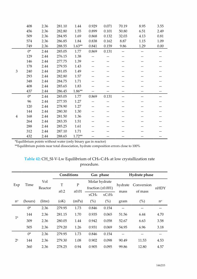
144/215

408 2.36 281.10 1.44 0.929 0.071 70.19 8.95 3.55

456 2.36 282.80 1.55 0.899 0.101 50.80 6.51 2.49

509 2.36 284.95 1.69 0.868 0.132 32.03 4.13 0.81

574 2.36 286.85 1.84 0.838 0.162 8.87 1.15 1.09

749 2.36 288.55 1.63** 0.841 0.159 9.86 1.29 0.00

3

0* 2.44 285.05 1.77 0.869 0.131 -- -- --

129 2.44 276.15 1.38 -- -- -- -- --

146 2.44 277.75 1.39 -- -- -- -- --

178 2.44 279.55 1.43 -- -- -- -- --

240 2.44 281.05 1.49 -- -- -- -- --

293 2.44 282.80 1.57 -- -- -- -- --

348 2.44 284.75 1.71 -- -- -- -- --

408 2.44 285.65 1.83 -- -- -- -- --

437 2.44 286.45 1.86** -- -- -- -- --

4

0* 2.44 285.05 1.77 0.869 0.131 -- -- --

96 2.44 277.55 1.27 -- -- -- -- --

120 2.44 278.90 1.27 -- -- -- -- --

144 2.44 280.30 1.30 -- -- -- -- --

168 2.44 281.50 1.36 -- -- -- -- --

264 2.44 283.35 1.51 -- -- -- -- --

288 2.44 285.25 1.61 -- -- -- -- --

312 2.44 287.10 1.71 -- -- -- -- --

432 2.44 288.65 1.72** -- -- -- -- --

*Equilibrium points without water (only binary gas in reactor)

**Equilibrium points near total dissociation, hydrate composition errors close to 100%

Table 42: CH_SI-V-Lw Equilibrium of CH4-C3H8 at low crystallization rate

procedure.

Exp Time Vol

Reactor


T

±0.2

P

±0.01

Molar hydrate

fraction (±0.001) hydrate

mass

Conversion

of mass nHDY

xCH4 xC3H8

no (hours) (litre) (oK) (mPa) (%) (%) gram (%) no

1b

0* 2.36 279.95 1.73 0.846 0.154 -- -- --

144 2.36 281.15 1.70 0.935 0.065 51.56 6.44 4.70

309 2.36 280.05 1.44 0.942 0.058 52.67 6.63 3.58

505 2.36 279.20 1.26 0.931 0.069 54.95 6.96 3.18

2b

0* 2.36 279.95 1.73 0.846 0.154 -- -- --

144 2.36 279.30 1.08 0.902 0.098 90.49 11.53 4.53

360 2.36 278.25 0.94 0.905 0.095 99.86 12.80 4.57

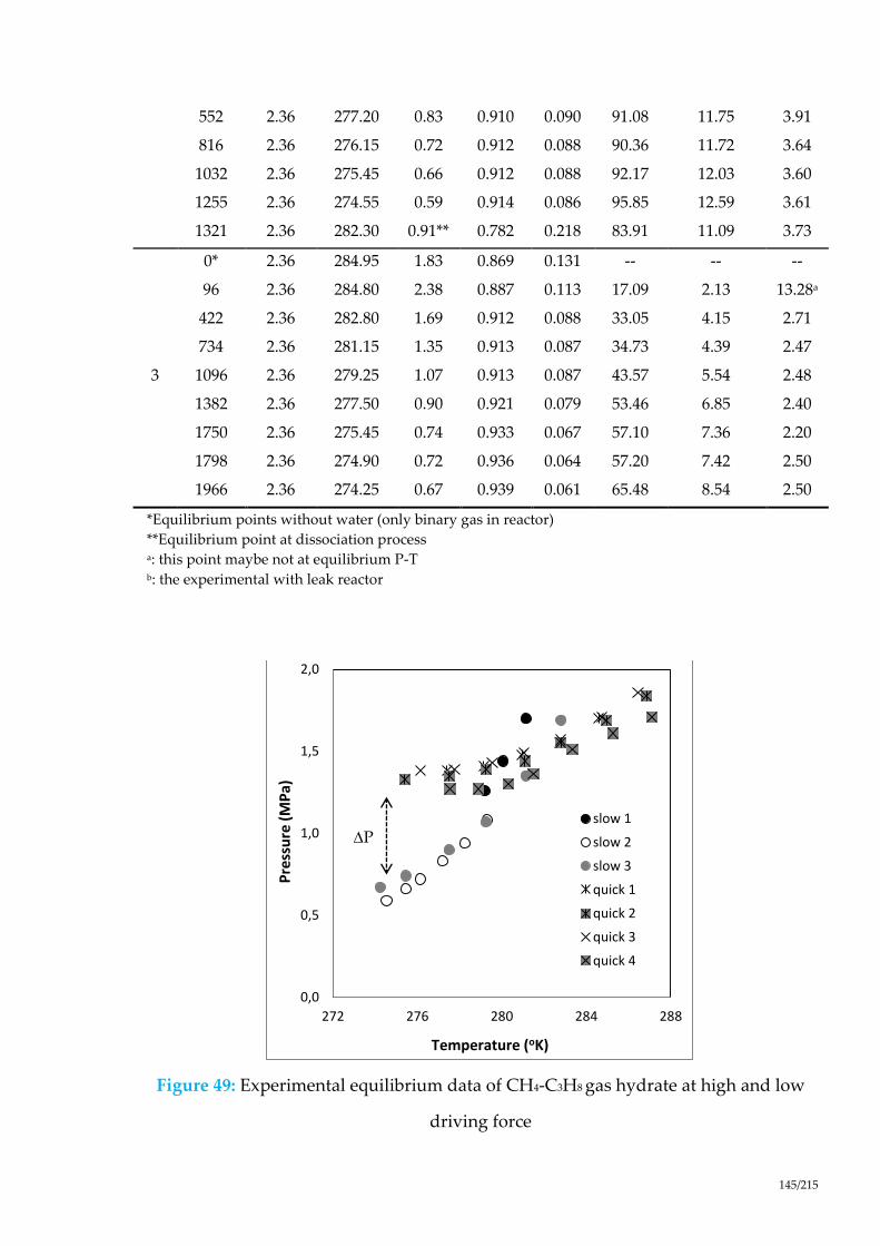
145/215

552 2.36 277.20 0.83 0.910 0.090 91.08 11.75 3.91

816 2.36 276.15 0.72 0.912 0.088 90.36 11.72 3.64

1032 2.36 275.45 0.66 0.912 0.088 92.17 12.03 3.60

1255 2.36 274.55 0.59 0.914 0.086 95.85 12.59 3.61

1321 2.36 282.30 0.91** 0.782 0.218 83.91 11.09 3.73

3

0* 2.36 284.95 1.83 0.869 0.131 -- -- --

96 2.36 284.80 2.38 0.887 0.113 17.09 2.13 13.28a

422 2.36 282.80 1.69 0.912 0.088 33.05 4.15 2.71

734 2.36 281.15 1.35 0.913 0.087 34.73 4.39 2.47

1096 2.36 279.25 1.07 0.913 0.087 43.57 5.54 2.48

1382 2.36 277.50 0.90 0.921 0.079 53.46 6.85 2.40

1750 2.36 275.45 0.74 0.933 0.067 57.10 7.36 2.20

1798 2.36 274.90 0.72 0.936 0.064 57.20 7.42 2.50

1966 2.36 274.25 0.67 0.939 0.061 65.48 8.54 2.50


**Equilibrium point at dissociation process a: this point maybe not at equilibrium P-T b: the experimental with leak reactor

Figure 49: Experimental equilibrium data of CH4-C3H8 gas hydrate at high and low

driving force

0,0

0,5

1,0

1,5

2,0

272 276 280 284 288

Pre

ssu

re (

MP

a)

Temperature (oK)

slow 1

slow 2

slow 3

quick 1

quick 2

quick 3

quick 4

P

146/215

Figure 49 shows four results at high crystallization rate and three at low driving

force. In both cases, the PT results are consistents. We can see that the pressure at

low temperature is significantly different from one procedure to another (7 bars

versus 14 bars for quick crystallization). Of course, experiments take more time at

low crystallization rate, wich could explain the pressure difference. However, a

pressure drop of 7 bars is quite significant (too big?), and this should be checked.

Some experiments to investigate the pressure drop due to the leak showed a

pressure drop of 4 bars in 13 days at 30 bars in the reactor. It is still too early to draw

a final concusion, but, the thermodynamic modelling could be a tool to investigate

CH4-C3H8 equilibria. If a look is taken at the first equilibria observed experimentally

(the leak is still not significant, the themodynamic model is not accurate for structure

SI or structure SII in predicting the pressure. So, either we did not observe a

thermodynamic equilibrium, or there is both structure of hydrate formed.

Nevertheless, a modelling takin into account the mass balance could deepen this

question (see chapter §8. Page. 151).

Table 43: Experimental and predicted pressures for the first data obtained in each

experiments (CH4-C3H8)

T

(K ±0.2)

P

(bars ±0.1)

Ppred

(SI)

Ppred

(SII)

1 274.90 14 24 6

2 274.90 14.3 25.5 6.6

1b 279.15 17 31.7 7.5

2b 278.30 10.8 20.3 5.2

3b 284.80 18.3 35.4 9.1

147/215

7.4. CH4-C2H4-C3H8 GAS MIXTURES

In this last section, an experiement from CH4-C2H6-C3H8 gas mixture is presented.

Unfortunatelly, this experiment suffered from the same leak problem.

If we compare the results at the same temperature (about 277 K as example), the

“equilibrium” pressure are 35.5 bars and 24 bars at quick and slow crystallization

rate respectively. A pressure difference of more than 10 bars if quite significant, and

we do think that the leak is responsible for such a difference.

As said before, others experiments are needed to confirm this observation.

Figure 50: Experimental equilibrium data of CH4-C2H6-C3H8 gas hydrate at low

driving force

0

1

2

3

4

5

273 276 279 282 285

pre

ssu

re (

mP

a)

Temperature (oK)

P-T at low procedure

P-T at quick procedure

148/215

Table 44 : CH_SI-V-Lw Equilibrium of CH4-C2H6-C3H8 at high crystallization rate (Le

Quang, 2013)

Exp Time Vol

Reactor


T

±0.2

P

±0.01

Molar hydrate fraction

(±0.001) hydrate

mass

Conversion

of mass nHDY

xCH4 xC2H6 xC3H8

no (hours) (litre) (oK) (mPa) (%) (%) (%) gram (%) no

1

0* 2.36 -- -- -- -- -- -- -- --

-- 2.36 275.35 3.13 0.98 0.003 0.017 -- -- 6

-- 2.36 276.15 3.36 0.98 0.003 0.017 -- -- 6.2

-- 2.36 277.15 3.55 0.98 0.004 0.016 -- -- 7.1

-- 2.36 277.85 3.67 0.98 0.006 0.014 -- -- 6.4

-- 2.36 279.25 3.78 0.97 0.008 0.022 -- -- 7.7

-- 2.36 280.75 3.94 0.97 0.012 0.017 -- -- 8.5

-- 2.36 282.15 4.21 0.96 0.017 0.023 -- -- 7.2

-- 2.36 283.15 4.34 0.96 0.019 0.021 -- -- 8.2

-- 2.36 284.15 4.5 0.95 0.022 0.028 -- -- 9.7


Table 45: CH_SI-V-Lw Equilibrium of CH4-C2H6-C3H8 at low crystallization rate

procedure.

Exp Time Vol

Reactor


T

±0.2

P

±0.01

Molar hydrate fraction

(±0.001) hydrate

mass

Conversion

of mass nHDY

xCH4 xC2H6 xC3H8

no (hours) (litre) (oK) (mPa) (%) (%) (%) gram (%) no

1b

0* 2.36 285.05 2.78 -- -- -- -- -- --

565 2.36 277.05 2.4 -- -- -- -- -- --

733 2.36 276.45 2.12 -- -- -- -- -- --

925 2.36 275.85 1.86 -- -- -- -- -- --

1164 2.36 274.80 1.59 -- -- -- -- -- --

1317 2.36 274.35 1.47** -- -- -- -- -- --


**Equilibrium point at dissociation process b: the experimental with leak reactor

149/215

7.5. CONCLUSION

The two procedures used suggest a kinetic influence on mixed hydrate formation

(mostly experiment on CO2-CH4-C2H6 gas mixture). Experimental results showed

that the enclathration of the heavier molecule (ethane) is more important at low than

high crystallization rate. Moreover, the equilibrium pressure for a given temperature

and initial gas composition, is different. This observation could not be supported by

all the measurments since a leak was detected concerning CH4-C3H8, and CH4-C2H6-

C3H8 gas mixtures. However, the pressure drop does not seem to be responsible for

the big differencies observed. New experiments have to be performed to confirm this

statement.

Also, the thermodynamic simulations are also in better accordance with the results

at slow crystallization.

In the end, the results show that mixed hydrate equilibrium could not be at

thermodynamic equilibrium. If the measurements are performed at high

crystallization rate the hydrate volume and composition will not be in accordance

with the thermodynamic modeling. This observation could have a significant impact

on design calculations in which the assumption of thermodynamic equilibrium is

made (leading to an over estimation of the hydrates volume in the pipe-lines).

New experimental are scheduled, we will be performed to confirm again the

conclusions in this work. The next section of this work, Flash calculation is going to

establish in up-grading our simulation software running equilibrium simulation by

adding a flash algorithm. The objective is to take into account the history of the

crystallization in the modelling work.

150/215

151/215

8. FLASH CALCULATION

8.1. INTRODUCTION

So far, mixed hydrate crystallization has been observed from experiments and

thermodynamic modeling. If the experiments have been performed at different

crystallization rate, there could be some issues and complications. Indeed, a

difference in the final state of the system has been discovered, but the exact order of

magnitude remains unreliable. That is why the thermodynamic modeling has been

used to support these conclusions. The thermodynamic modeling has given good

results on CO2-CH4-C2H6 experiment (deviation on pressure <5%, and <24% on

hydrate composition). However, it is difficult to draw an ultimate conclusion based

on this sole comparison. Actually, the thermodynamic modeling only predicts the

composition of the first nucleus in solution (liquid-hydrate equilibrium LHE).

Experimentally, this composition can hardly be measured. That is why a significant

volume of hydrate is experimentally formed to measure this hydrate composition

with more accuracy. But, if we consider that the hydrate composition is not

stoichiometric, the measured (and calculated) hydrate composition is only an

average value. It is not the case in the thermodynamic modeling. Hence, it is difficult

to compare the thermodynamic model with the experimental results, and the

crystallization process has to be taken into account in the calculations.

Another issue considered previously (section thermodynamic) is the regression of

Kihara parameters. Usually, these parameters are calculated from experimental

results (PT data). At best, only pure hydrates are used, for example pure CO2

hydrate to compute CO2 parameters. However, this is not always possible (Le

Quang, 2013; Le Quang et al., 2016). In this situation, mixed hydrate results can be

used. From these results, the objective function can be the error between equilibrium

and predicted pressure, as well as the difference between the experimental and

predicted hydrate composition. But, two issues arise: the experiments could not be

performed at thermodynamic equilibrium, and the measured hydrate composition

could be only an average value. To obtain more reliable Kihara parameters, it would

be very interesting to be able to predict the hydrate volume, and the hydrate

composition, taking into account the non-stoichiometry of the hydrate phase.

At last, the hydrate volume to be formed is essential to determine the amount of

kinetic inhibitors (KHI) to use in flow-assurance.

Therefore, flash calculation algorithms have been developed in the hydrate team, to

combine both thermodynamic modeling and mass balance while calculating phase

equilibria.

152/215

8.2. STATE OF THE ART

There are not many studies that take into account the crystal growth of mixed

clathrate hydrates. Usually, the hydrate phase is considered to be homogeneous, at

thermodynamic equilibrium with the surrounding fluid phase. To find such studies,

we have to look for kinetic models. Recently, (Herri and Kwaterski, 2012) suggested

a kinetic model, already presented in section §5.5 Page.95. More recently, a kinetic

flash algorithm has been presented by (Boesen et al., 2014). As a kinetic approach,

time is a variable. The driving force is given by the (Per Skovborg and Rasmussen,

1994; P. Skovborg and Rasmussen, 1994). However, this last model does not appeal

to thermodynamic equilibrium equations.

8.2.1 USUAL FLASH CALCULATIONS

In thermodynamics, flash calculations are thermodynamic equilibrium equations

resolution combined with mass balance (and eventually energy balance) equations.

Gibbs phase law gives the degree of freedom of a thermodynamic system. Usually,

this number is higher than two:

𝑣𝑎𝑟 = 𝑛𝑢𝑚𝑏𝑒𝑟 𝑜𝑓 𝑐𝑜𝑚𝑝𝑜𝑛𝑒𝑛𝑡𝑠 – 𝑛𝑢𝑚𝑏𝑒𝑟 𝑜𝑓 𝑝ℎ𝑎𝑠𝑒𝑠 + 2 (130)

var = numberofcomponents– numberofphases +Among the intensive parameters,

pressure (P) and temperature (T) are usually chosen. The volume of the system can

also replace one of these two properties. A Flash calculation at given temperature

and pressure is often called Flash PT. If there is a heat exchange, the quantity of

energy Q can be used (Flash QP, flash QT…). An energy balance is then necessary.

More details can be found in the literature on flash calculations (Michelsen, 1990a,

1990b). A basic algorithm is drawn on Figure 51.

153/215

Figure 51: Example of Flash algorithm (θ=mass flow ratio between phases)

This figure shows that there are two loops in standard flash calculations:

- One loop on mass balance verification (θ),

- One loop on thermodynamic equilibrium (Kij).

where symbol θ stands for the global mass ratio between the two phases (usually

liquid/vapor).

8.2.2 FLASH HYDRATE MODELING

In the case of hydrate flash calculations, the algorithm is more complicated, since

there are three phases at equilibrium. The third phase (hydrate) decreases the degree

of freedom by one. To fit to the experiments of this work, and more extensively to

batch experiments, the volume is then considered to be constant. Then, since the

temperature is set (cryothermostat), this is the variable for the modeling.

Iteration for

determination of θ

Initialisation

(T0, P0, x0, y0, θ)

Initial partition

coefficient (Kij)

Mass Balance:

Calculation of θ

Is Thermodynamic

equilibrium checked ?

Calculation

Kij(T,p,x,y)

The end :

Tf, Pf, xf, yf, θ

No

154/215

The other issue is the supposed non-stoichiometry of the hydrate crystal. If the solid

phase is not homogeneous, the model will have to take into account the

crystallization, and the thermodynamic path of the system.

Therefore, the only solution to consider the crystal growth in thermodynamic

modeling is to perform successive flash calculation along the crystallization. The

basic algorithm is represented on Figure 52. This figure shows that the crystallization

is discretized into successive flash calculations. Each step corresponds to a new mass

of hydrate. This mass (combined with cavity occupancy) is considered with van der

Waals and Platteuw as described in section §4, Page.57. There are two options for the

former mass of hydrate:

- It remains the same,

- It is reorganized to be at thermodynamic equilibrium with the surrounding

liquid phase.

These two options lead to two different algorithms, two frameworks for the hydrate

flash calculations. After presenting the basic algorithm, these two frameworks will

be described.

8.3. BASIC ALGORITHM

The number of degree of freedom is only one. To compare the further simulations to

the previous experiments, the temperature is chosen as variable. The volume is

constant, since it is the reactor volume.

The basic algorithm is represented on Figure 52. The objective is to simulate the

thermodynamic path of the crystallization, from the initial state (vapor liquid

equilibrium, at high temperature), to the final state (hydrate-liquid-vapor

equilibrium) at a lower, and final, temperature. Figure 53 shows what is to be

simulated. There are two stages: VLE, when the temperature is too high for the

hydrate phase to form, and vapor-liquid-hydrate equilibrium (VLHE), at lower

temperatures. Point A represents the initial state (P0, T0). Point B corresponds to the

first three phase equilibrium (VLHE) when decreasing the temperature (TB). Step A

to B is the first stage. In the model, this is VLE combined with mass balance. That is

to say, a standard vapor-liquid flash calculation

155/215

Figure 52: Basic hydrate flash algorithm.

Then, the successive Ci points correspond to the second stage, when the temperature

decreases (VLHE, when TC<TB). Since there is a mass transfer from the gas phase to

the hydrate phase (through the liquid phase), the gas molecules are consumed in

time. The changes in the gas composition modify the liquid-hydrate equilibrium.

This is why there is no longer only one LHE equilibrium curve. Each Ci point

belongs to a different LHE curve. The numbers of Ci points depends on the

discretization of the crystallization. It is an input number, written N (and 𝑖 ∈

{1, … , 𝑁}). The temperature step is then:

dm

adjustment

Initialisation

(T0, P0, x0, y0, θ)

Initial partition coefficients

(Kij)

Mass Balance:

Calculation of θ

Is Thermodynamic

equilibrium checked ?

Calculation

Kij(T,P,x,y)

The end :

Tf, Pf, xf, yf, θ

No

Yes

Crystallization

𝑚𝑖𝐻 = 𝑚𝑖−1

𝐻 + 𝑑𝑚

No

Yes

T=Tf ?

i=i+1

No

Yes

156/215

∆𝑇 =

𝑇𝐵 − 𝑇𝐷

𝑁 (131)

The higher N is, the more continuous the crystallization is. The lower this is, the

more the driving force is significant in the model.

In the end (at final temperature Tf=TD), the system reaches the final state of

equilibrium.

The inputs need to account for the total mass of the system. The same procedure as

the experimental one is simulated in the modeling. First, “injection” of the gas

mixture (gas composition and pressure). The mass of each gas molecule is calculated

with the use of an equation of state (SRK). Then, a given mass of water is added.

Then, the final temperature is chosen. In the end, the inputs are:

- Initial temperature and pressure (𝑇0 𝑎𝑛𝑑 𝑃0),

- the “reactor” volume (𝑉𝑅),

- gas mixture composition (𝑧0𝐺),

- the mass of water (𝑚𝑤),

- the final temperature (𝑇𝑓),

- the iterations number N.

Figure 53: Thermodynamic path (Bouillot and Herri, 2016).

157/215

8.4. HYDRATE FLASH ALGORITHM WITHOUT CRYSTAL REORGANIZATION

In this section, details on the framework for the hydrate flash calculation without the

crystal reorganization are suggested. The detailed algorithm is described on Figure

54.

The first part corresponds to the VLE flash algorithm. In the model, the gas phase is

modeled with SRK equation of state (gas density). The vapor-liquid equilibrium is

calculated with Henry’s law like equation (see also at section §6.4.3. Page. 129). Two

loops are used in this first step. The following simultaneous equations are

considered:

{

𝑛𝑗0 = 𝑛𝑗

𝑉 + 𝑛𝑗𝐿

𝑛𝑗𝐿 =

𝑉𝐿𝜌𝑤𝑜

𝑀𝑤

𝑧𝑗𝜑𝑗

𝐺𝑃

𝐾𝐻,𝑗∞

(132)

Where n is the quantity (mole) of molecule j in phase vapor or liquid or both

(superscripts V, L and 0, respectively). 𝑛𝑗𝑉(𝑇, 𝑃, 𝑧𝑗 , 𝑉) is calculated with SRK EoS.

𝜑𝑗𝐺 , the fugacity coefficient of the vapor phase can be set to 1 for hydrocarbon gas

mixtures. Since the final adjustment variable is P, the VLE flash determines the

equilibrium pressure of the system (then marked 𝑃𝑉𝐿𝐸).

After this initial VLE flash calculation, the pressure 𝑃𝑉𝐿𝐸 of the system is known.

Then, the temperature is decreased to reach the three phase equilibrium, that is to

say, VLE flash combined with LHE equations. The output of VLE flash is 𝑃𝑉𝐿𝐸 , and

the output of LHE is also a pressure (then marked 𝑃𝐿𝐻𝐸). The three phases

equilibrium is reached when 𝑃𝑉𝐿𝐸 = 𝑃𝐿𝐻𝐸.

From this point, the crystallization begins. System is at three phases equilibrium, but

only vapor and liquid phases coexist. As said in introduction, two hypotheses on the

hydrate phase can be considered: homogeneous and heterogeneous composition. In

this first section, the non-stoichiometric approach is considered.

To reach the final state, the crystal growth is examined. There is a discretization of

this growth, depending on the number of iterations N. If N is high enough, the

growth can be considered as continuous (very low ∆𝑇). Otherwise, the driving force

taken into account in the crystallization process is more significant. Figure 55 shows

the crystallization modeling.

Since the crystal growth is discretized through ∆𝑇 step, there is a ∆𝑚𝐻 mass of

hydrate that corresponds to the previous variation. This mass (more specifically the

158/215

mass of water that has crystallized ∆𝑚𝑤𝐻) is the new adjustment variation in solving

the following simultaneous equation system:

{∀𝑗 , 𝑛𝑗

0 = 𝑛𝑗𝑉 + 𝑛𝑗

𝐿 + 𝑛𝑗𝐻

𝑃𝑉𝐿𝐸 = 𝑃𝐿𝐻𝐸 (133)

𝑛𝑗𝑉 is calculated using SRK EoS, 𝑛𝑗

𝐿 using Henry’s law like equation (section §6.4.3.

Page. 129), and 𝑛𝑗𝐻 from (van der Waals and Platteeuw, 1959) (as described in section

§4. Page. 57) combined with assumed ∆𝑚𝐻 value. This last calculation is the tricky

one. The procedure is the following one.

First, a mass of water that has crystallized (∆𝑚𝑤𝐻) is taken as hypothesis. From this

mass, the corresponding volume of hydrate is calculated. To do so, the empty

hydrate density is used (the hydrate with no gas molecules inside). This density

depends on the hydrate structure. In this thesis, only structure I and II are

investigated (𝜌𝐼𝐻−𝛽

and 𝜌𝐼𝐼𝐻−𝛽

). (Sloan and Koh, 2007) give an expression for the

density of hydrates which is presented in section §2.2.2, Page. 31:

𝜌𝐻 =

𝑁𝑤𝑀𝑤 + ∑ ∑ 𝜃𝑖𝑗𝑣𝑖𝑀𝑗𝑛𝑖=1

𝐶𝑗=1

𝑁𝐴𝑣𝑜𝑉𝑐𝑒𝑙𝑙 (134)

Where 𝑁𝑤 is number of water molecule per unit cell (see Table 1), 𝑁𝐴𝑣𝑜 the

Avogadro’s constant, 𝑀𝑤 and 𝑀𝑗 the molecular weights of water and molecule j, 𝑣𝑖

the number of type i cavities by component j, 𝜃𝑖𝑗 the fractional occupation of cavity i

by component j, and 𝑉𝑐𝑒𝑙𝑙 the volume unit cell (Table 1).

159/215

Figure 54: Algorithm to perform hydrate flash calculation with no reorganization of

the crystal phase (framework I) (Bouillot and Herri, 2016).

For an empty hydrate, this formula becomes:

𝜌𝐻−𝛽 =

𝑁𝑤𝑀𝑤

𝑁𝐴𝑣𝑜𝑉𝑐𝑒𝑙𝑙 (135)

Values of 790 and 785 kg/m3 can be obtained for structure I and II respectively.

From these values, the crystallized volume of hydrate is:

160/215

∆𝑉𝐻 =

∆𝑚𝑤𝐻

𝜌𝐻−𝛽 (136)

From ∆𝑚𝑤𝐻 value, the mass of gas in the hydrate cavities, or 𝑛𝑗

𝐻, is fully determined

(thanks to occupancy 𝜃𝑖𝑗). Also, the volume of the aqueous phase is known (𝑉𝐿 =

𝜌𝑤𝐿 𝑚𝑤

𝐿 by assuming pure water and 𝜌𝑤𝐿 = 1000 𝑘𝑔/𝑚3), as well as the vapor phase

volume (𝑉𝑉 = 𝑉𝑅 − 𝑉𝐿 − 𝑉𝐻).

A “VLE flash” is then performed, and the resulting pressure 𝑃𝑉𝐿𝐸 is compared to the

predicted LHE pressure (𝑃𝐿𝐻𝐸). If 𝑃𝑉𝐿𝐸 ≠ 𝑃𝐿𝐻𝐸, the ∆𝑚𝑤𝐻 value is not correct. There is

then an iterative process to find the right hydrate volume, or mass. The objective

function is:

𝐹𝑜𝑏𝑗(𝑑𝑚𝑤

𝐻) =|𝑃𝑉𝐿𝐸 − 𝑃𝐿𝐻𝐸|

𝑃𝑉𝐿𝐸→ 0 (< 10−3) (137)

Once the right value of ∆𝑚𝑤𝐻 (or 𝑑𝑚𝑤

𝐻) is found, the temperature of the system is

decreased of ∆𝑇, and the calculations start over until 𝑇 = 𝑇𝑓.

Figure 55: Mixed hydrate growth (no reorganization) (Bouillot and Herri, 2016).

The most important hypothesis in this part comes from the calculation of 𝜃𝑖𝑗 and its

use in calculating 𝑛𝑗𝐻. Indeed, either the occupancy is calculated from the initial

161/215

equilibrium state (before the temperature decrease), or after. The first hypothesis

leads to a hydrate phase that is not at thermodynamic equilibrium with the

surrounding liquid phase after crystallization, while it is the case in the second

hypothesis. Of course, if the number of iteration in infinite, the approaches are the

same. In this algorithm, the first approach is chosen (marked framework I). The

second (framework II) is investigated in next section.

8.5. HYDRATE FLASH ALGORITHM WITH CRYSTAL REORGANIZATION

In this algorithm, then called framework II, the last layer of the hydrate crystal is at

thermodynamic equilibrium with the surrounding liquid. To check this assumption,

the equilibrium equation has to be validated through the occupancy factor θ. Figure

56 presents the algorithm with hydrate reorganization.

Figure 56: Algorithm to perform hydrate flash calculation with reorganization of the

hydrate phase during crystallization (framework II) (Bouillot and Herri, 2016).

On this figure, a new loop is added to the initial algorithm. In the end of each

iteration i, the occupancy factor 𝜃𝑗𝑖 is calculated after crystallization (of 𝑑𝑚𝑤 ) and

compared before 𝑑𝑚𝑤 adjustment. This way, the LHE equation is validated after

162/215

crystallization, for an occupancy factor in accordance with (van der Waals and

Platteeuw, 1959) theory at the equilibrium with the fluid phase’s compositions.

As with the algorithm with no hydrate phase reorganization, the crystallization is

discretized. Figure 53 also represents the thermodynamic path. If the number of

iteration is infinite, we can expect that the occupancy factor before and after

crystallization is the same. This is why the two algorithms are converging when 𝑁 →

∞.

If the number of iteration is just 1, there is only one step in the hydrate growth, and

the hydrate phase is completely homogeneous. This approach is then called

framework II*, and is represented in Figure 57.

Figure 57: Hydrate growth with crystal phase reorganization (framework II*)

(Bouillot and Herri, 2016).

8.6. KIHARA PARAMETERS OPTIMIZATION

To investigate the hydrate flash algorithm, an estimation of the Kihara parameters

was needed. Since the used code (MATLAB) is different than is the previous

modeling work (use of GasHyDyn), the Kihara parameters are also different. Table

46 gives the Kihara parameters obtained from this optimization.

163/215

Table 46: Quick Kihara parameters optimization of CO2, CH4 and C2H6 on a few

experimental data (Adisasmito et al., 1991; Avlonitis, 1988; Dyadin, 1996; Y. A.

Dyadin et al., 1996; Yurii A. Dyadin et al., 1996; Englezos and Bishnoi, 1991; Larson,

1955; Le Quang et al., 2016; Nixdorf and Oellrich, 1997; Thakore and Holder, 1987;

Yasuda and Ohmura, 2008) (* data from (Sloan and Koh, 2007))

𝜺/𝒌 𝝈 a* RMSE Nb. Data

CO2 171.78 2.978 0.6805 0.02 8

CH4 160.70 3.101 0.3834 2.43 14

C2H6 176.83 3.220 0.5651 0.062 18

8.7. RESULTS

To investigate the frameworks and compare them to experimental results, a

reference case is used. This baseline is a CO2-CH4-C2H6 gas mixture, presented

previously (Table 19) and published in Fluid Phase Equilibria (Le Quang et al., 2016).

It is chosen because it is an experiment at low crystallization rate, supposed to be as

close as possible to thermodynamic equilibrium during crystallization.

Then, an investigation of the uncertainty of the model due to Kihara parameters

uncertainties is suggested.

In the end of this section, a comparison with experiments at high crystallization rate

will be presented.

8.7.1. THERMODYNAMIC EQUILIBRIUM

First, the thermodynamic model in the hydrate flash frameworks is compared to the

reference case. Table 47 and

Figure 58 show that the thermodynamic model provides results in accordance with

the experimental results (RMSE of 0.31 for the pressure, and lower than 0.04 for the

hydrate composition). The LHE part of the flash algorithm is accurate in this case,

assuming a SI structure. SI structure will then be considered in next sections.

164/215


C2H6) from classic thermodynamic calculations assuming a SI structure.

T P exp Exp. Gas composition

(%mol)

Exp. Hydrate composition

(%mol)

P

pred

Pred. Hydrate

composition (%mol)

(K) (bars) CO2 CH4 C2H6 CO2 CH4 C2H6 (bars) CO2 CH4 C2H6

279.35 41.7 0.037 0.943 0.02 0.117 0.669 0.214 41.1 0.0569 0.8598 0.0833

277.75 37.75 0.035 0.951 0.014 0.081 0.799 0.12 36.39 0.0579 0.8801 0.0619

277.35 35.6 0.034 0.952 0.014 0.081 0.828 0.091 35.09 0.0566 0.8828 0.0605

276.4 31.8 0.033 0.957 0.01 0.075 0.849 0.076 32.79 0.0567 0.8977 0.0456

275.6 30.4 0.031 0.959 0.01 0.076* 0.854* 0.070* 30.35 0.0546 0.8996 0.0458

274.45 27.6 0.03 0.963 0.007 0.075 0.862 0.063 27.54 0.0534 0.9093 0.0373

RMSE: 0.31 0.0129 0.0383 0.0256

Figure 58: PT diagram of experimental and predicted results of the reference case

(CO2-CH4-C2H6) at different temperatures from the same initial state.

165/215

8.7.2. FLASH RESULTS

Results obtained for the two frameworks and different iteration numbers N is

suggested in Table 48. Thermodynamic paths for each framework and different

number of iterations are presented on Figure 58.

First, all the frameworks provide three phase equilibrium (VLHE) at the same

temperature and pressure (280.14 K and 42.63 bars). This means that the first crystal

in the bulk should appear in these conditions. At a lower temperature (T<280.14 K),

the crystal phase grows. This is point B on Figure 53.

Then, the temperature is decreased step by step (Ci points), until it reaches the final

temperature Tf=274.5 K. This is the final experimental temperature.

Figure 58 presents the thermodynamic path (both experimental and predicted) of the

crystallization, i.e. temperature-pressure states during the crystallization. This figure

also provides the thermodynamic LHE curves that are crossed at each step during

the crystallization (N=7 and structure SI). This figure is in accordance with Figure 53

and shows a good agreement between the experimental and predicted results

concerning the pressure.

More specifically, Table 48 shows that the deviation between experimental and

simulated results is under 8% (both hydrate volume and final pressure at the same

time).

As expected, framework I and II converge when 𝑁 → ∞ (continuous crystallization,

see N=100 as example). Then, using “only” 20 iterations for frameworks I and II

allows the calculation of a continuous crystallization (results close to N=100) while at

the same time presenting a lower time consumption in the calculations.

Then, frameworks I and II provide accurate results in pressure and hydrate volume

(<5%). The lower deviation obtained is for framework II for 8 iterations. Concerning

influence of N for framework I, the more the discretization is significant, the lower

the deviation is. For framework II, it is the opposite. If a few iterations are used (n =

3), the accuracy deteriorates. This can also cause the calculation of negative

compositions (too many gas molecules into the hydrate phase, and a negative

number in the gas phase).

At last, the framework II* results are not in better accordance with experimental

data. The final pressure is closer, but not the hydrate volume (higher).

166/215

Tab

le 4

8: E

xp

erim

enta

l v

ersu

s p

red

icte

d r

esu

lts

for

the

refe

ren

ce c

ase

(CO

2, C

H4

and

C2H

6)

fro

m c

lass

ic t

her

mo

dy

nam

ic c

alcu

lati

on

s a

ssu

min

g a

SI

stru

ctu

re.

dev

.

(%)

(±0.

01)

Ex

p.

10.6

5.9

4.3

3.7

3.5

3.5

2.0

2.9

3.2

3.9

3.9 0

hy

dra

te c

om

po

siti

on

(%m

ol)

(±0

.003

) xC

2H6

0.09

6

0.08

2

0.07

9

0.07

7

0.07

7

0.07

6

0.07

3

0.07

5

0.07

6

0.06

1

0.06

1

0.06

2

xC

H4

0.83

1

0.84

5

0.84

9

0.85

1

0.85

2

0.85

2

0.85

6

0.85

4

0.85

3

0.87

1

0.87

1

0.86

2

xC

O2

0.07

3

0.07

3

0.07

2

0.07

2

0.07

2

0.07

2

0.07

1

0.07

1

0.07

2

0.06

9

0.06

9

0.07

5

nH

(±0.

001

)

(mo

l)

1.04

5

1.11

7

1.14

0

1.14

9

1.15

3

1.15

3

1.17

5

1.16

2

1.15

8

1.26

3

1.26

3

1.21

Gas

co

mp

osi

tio

n

(%m

ol)

(±0

.001

) xC

2H6

-0.0

04

0.00

0

0.00

1

0.00

2

0.00

2

0.00

2

0.00

3

0.00

2

0.00

2

0.00

8

0.00

8

0.00

7

xC

H4

0.97

2

0.96

9

0.96

8

0.96

8

0.96

7

0.96

7

0.96

6

0.96

7

0.96

7

0.96

1

0.96

1

0.96

3

xC

O2

0.03

1

0.03

1

0.03

1

0.03

1

0.03

1

0.03

1

0.03

1

0.03

1

0.03

1

0.03

1

0.03

1

0.03

0

nG

(±0.

001)

(mo

l)

2.16

6

2.09

8

2.07

6

2.06

7

2.06

3

2.06

4

2.04

2

2.05

5

2.05

9

1.95

8

1.95

8

2.00

9

con

v.

(±0.

01)

%m

ass

13.9

1

14.9

9

15.3

4

15.4

7

15.4

9

15.5

3

15.8

6

15.6

7

15.4

8

17.1

1

17.1

0

15.9

9

𝒎𝒘𝑯

(±

0.01

)

(g)

111.

43

119.

38

122.

05

123.

05

123.

51

123.

51

125.

98

124.

55

124.

05

135.

94

135.

93

127.

10

Pf

(±0.

01)

(bar

s)

30.0

3

29.1

8

28.9

0

28.7

9

28.7

4

28.7

4

28.4

7

28.6

2

28.6

8

27.3

9

27.3

9

27.6

0

n

3*

5 10

20

50

100 8 20

100 5 20

I I I I I I II

II

II

II*

II*

Exp

.

167/215

Figure 59: Predicted and experimental thermodynamic paths (Pressure vs

temperature during crystallization) in the reference case (left: all frameworks at

different numbers of iterations; right: framework I, N=7).

8.8. KIHARA UNCERTAINTIES

Since Kihara parameters are very dependent on the authors as pointed by (Herri et

al., 2011), this is interesting to evaluate the influence of their uncertainties. To do this

investigation, Monte Carlo simulation were used.

1000 simulations were performed (each time) on the reference case from Gaussian

distribution around the mean values of 𝜀/𝑘 and 𝜎. Standard deviations were taken

from 1% to 5%. Framework I with 8 iterations was used.

Table 49 provides the obtained results. This demonstrates that a small difference

(5%) can have a significant effect on the final pressure and hydrate volume (standard

deviations of 42% and 125% respectively).

Since the models deviations from experimental results are usually under 5%, it can

be concluded that the frameworks are in good accordance with the experiments.

Table 49: Influence of the Kihara parameters uncertainties on the flash hydrate

results (framework I, reference case).

Pf σ(Pf ) σ(Pf) V^H σ(V^H) σ(V^H)

uncert. bars bars % mL mL %

1% 30.6 4.7 15.36 162 56 34.57

2% 31.20 8.06 25.83 152.3 98 64.35

3% 31.55 10.4 32.96 145.7 128.5 88.19

5% 32.05 13.4 41.81 138.6 172.9 124.75

168/215

8.9. MIXED HYDRATE CRYSTALLIZATION

In this last section, more experimental results are compared to simulated results.

These experimental data were obtained at high crystallization rate from CO2-CH4

and CO2-CH4-C2H6 gas mixtures (Le Quang et al., 2016). The objective is to

investigate if the results at high crystallization rate can be simulated with good

accordance with hydrate flash frameworks.

Experiments at high crystallization rate are expected to occur at non-thermodynamic

equilibrium. This is why framework II* should not be the best approach. Table 48

provides the aforementioned results.

Surprisingly, all frameworks give quite accurate results compared to experiments.

Expect framework II* (as expected), final pressure deviations are below 5%.

Concerning the final hydrate volume (or 𝑚𝑤𝐻), the deviation from the experimental

results is higher, but within the 3% uncertainty (± standard devivation σ) on the

kihara parameters (or within 1% uncertainty at ± variance). Since a kinetic effect on

the hydrate crystallization was anticipated, higher deviations were prophesied.

In conclusion, it seems that CO2-CH4 gas mixtures are not very much affected by

kinetics. Also, framework I with 5 iterations provides the best results. This

framework, combined with this number of iterations, was not the best as compared

to the reference case at slow driving force. This could validate that a higher driving

force is closer to framework I with no hydrate reorganization. Nevertheless, the

results are more than adequate, and it would probably not be the same for other

mixtures where kinetics could be predominating.

169/215

Tab

le 5

0: F

ram

ewo

rk I

(n

=5 a

nd

20)

an

d I

I* p

red

icti

on

s co

mp

ared

to

ex

per

imen

tal

resu

lts

at q

uic

k c

ryst

alli

zati

on

(g

as

1-2

fro

m C

O2-

CH

4 m

ixtu

res

and

3-4

-5 f

rom

CO

2-C

H4-

C2H

6 m

ixtu

res)

an

d s

low

cry

stal

liza

tio

n (

refe

ren

ce c

ase

of

the

pre

sen

t st

ud

y)

Fra

mew

ork

I, n

=20

dev

𝒎𝒘𝑯

(%)

(± 0

.1)

21.0

8.

2 --

--

22.0

3.2

Fra

mew

ork

II*

d

ev 𝒎

𝒘𝑯

(%)

(± 0

.1)

22.0

9.2 --

--

28.0

6.9

dev

Pf

(%)

(± 0

.1)

5.0

3.1

2.9

3.3

4.3

4.3

dev

Pf

(%)

(± 0

.1)

5.9

3.4

2.4

5.8

8.8

0.08

𝒎𝒘𝑯

pre

d

(g)

(± 0

.04)

256.

0 18

6.11

13

9.9

43.1

333.

5

123.

1

𝒎𝒘𝑯

pre

d

(g)

(± 0

.04)

259.

0

187.

9

155

49.3

349.

5

135.

9

Pf

pre

d

(bar

)

(± 0

.1)

31.6

28

.19

31.5

9 26

.21

33.8

7

28.7

9

Pf

pre

d

(bar

)

(± 0

.1)

31.3

28.1

29.9

5 25

.53

32.3

27.3

9

Exp

erim

enta

l

𝒎𝒘𝑯

(g)

(± 0

.04)

212.

0 17

2.1

--

--

272.

8

127.

1

Fra

mew

ork

I, n

=5

𝒎𝒘𝑯

(g)

(± 0

.04)

21.0

7.8 --

--

22.0

6.1

VH

(mL

)

( ±

0.04

)

268.

4 21

7.8

--

--

345.

3

160.

9

VH

(mL

)

( ±

0.04

)

5.0

2.9

4.2

3.3

4.3

5.8

Pf

(bar

)

(± 0

.1)

33.3

29

.1

30.7

27

.1

35.4

27.6

Pf

(bar

)

(± 0

.1)

255.

5

185.

4

135.

9 43

.0

333.

1

119.

4

Tf

(°C

)

(± 0

.1)

3.4

2.2

2.2

1.0

2.75

1.3

Tf

(°C

)

(± 0

.1)

31.7

28.2

6

32.0

26

.2

33.8

8

29.2

Gas

Gas

1

Gas

2

Gas

3

Gas

4

Gas

5

Gas

6

Gas

Gas

1

Gas

2

Gas

3

Gas

4

Gas

5

Gas

6

170/215

8.10. CONCLUSION

In this last chapter, a preliminary approach through flash calculation has been

suggested. Since it is a hard task to perform experiments at low crystallization rate

(very long experiments, subjects to apparatus issues), the modeling work can

suggest another comprehensive approach of hydrate crystallization.

The chosen approach has been a thermodynamic flash modeling. The model

presents different possible algorithms to take into account different mixed hydrate

growths (crystal phase reorganization, heterogeneous crystal or homogeneous

crystal phase).

In frameworks I and II, the crystallization is discretized in mass of hydrate. Crystal

growth is supposed to occur at local thermodynamic equilibrium with the

surrounding liquid (itself at thermodynamic equilibrium with the surrounding gas

phase). That is to say, successive thermodynamic equilibria between liquid and the

last layer of the hydrate phase are considered. These equilibria are considered before

layer crystallization for framework I, and after for framework II. The discretization

corresponds to the aforementioned layers of the hydrate crystal. As a consequence,

the final clathrate is non-stoichiometric.

In a slightly different physical approach with a single iteration (framework II*), the

hydrate phase is completely homogeneous (local composition = global composition).

To accomplish this, the crystal composition is homogenized during crystallization at

each step.

The simulation results, compared to a reference case (experiment at low

crystallization rate from CO2-CH4-C2H6 gas mixture), are pretty accurate. All the

frameworks provide deviations on final pressure and hydrate volume under 5%.

Frameworks I and II give better results in terms of crystallized mass of water while

framework II* seems to be better at predicting the final pressure. Also, a study on the

uncertainties due to Kihara parameters uncertainties showed that the experimental

results are within the margin of error for the models (about 15% and 35%

uncertainties on pressure and volume for 1% uncertainty on Kihara parameters).

Concerning the discretization of the crystallization, a number above 20 iterations for

the crystal growth is enough (frameworks I and II). As suspected, frameworks I and

II converge when the iteration number is infinite.

It is important to notice and underline that these flash calculations are only based on

thermodynamic equilibria. If different paths are investigated, then no kinetic

considerations exist such as mass transfer limitation at gas/liquid interface (Herri et

al., 1999a, 1999b), or possible diffusion effects at the liquid/hydrate interface (Herri

and Kwaterski, 2012). These considerations might be necessary to model hydrate

171/215

crystallization at high driving force, where the final pressure could to be

significantly affected.

In the end, the presented frameworks provide a usefull tool for industry and

academia to predict with a more realistic accuracy the final pressure. They also give

good orders of magnitude concerning the hydrate volume to be formed. For gas

mixtures that do not show important kinetic effects (such as CO2-CH4), predictions

are still accurate and within the same uncertainties.

If the kinetic effects of the crystallization rate on the final state of mixed hydrate

crystallization have not been proved yet from the experiments performed in this

thesis, the modeling of the mixed hydrate growth supports the hypothesis of this

work. This is also encouraging for future works.

172/215

173/215

9. CONCLUSION

In this thesis, an experimental and modeling work have been carried out to study the

influence of the crystallization rate on mixed clathrate hydrate formation. Since the

beginning of the study, mixed hydrates were suspected not to form at

thermodynamic equilibrium. Could mixed hydrate formation could be the results of

kinetic phenomena? This suggestion has a significant impact on the water

conversion and hydrate volume, two properties of high interest.

Therefore, two experimental protocols to mixed hydrate formation have been

presented: under low (cooling 0.2°C/day) and high rate of crystallization (cooling

10°C in one day). Experiments in an instrumented batch reactor have been

performed according to the two methods of crystallization. With this apparatus, the

gas and hydrate compositions could be measured, as well as the final pressure and

water conversion. Gas mixtures have been chosen to be representative of the oil

industry (from N2, CO2, CH4, C2H6 and C3H8).

Then, a modeling approach, from classic van der Waals and Platteuw method, has

been used to validate the assumption, as well as to investigate different hypothesis.

Moreover, in order to be able to calculate the hydrate volume, a flash calculation

approach has been used according to two different hypotheses (homogeneous and

heterogeneous hydrate crystal)

First, in the case of a binary mixture like N2/CO2, the thermodynamic modeling is

accurate, and the hydrate formation does not seem to be significantly affected by the

crystallization rate.

In the case of a ternary mixture like CO2/CH4/C2H6, differences between the results

have been observed in terms of hydrate composition, hydrate volume and final

pressure, from a same mixture and initial state. The final pressure at low

crystallization rate has been found to be lower than at high crystallization rate. The

occupancy of the hydrate cavities is fore significant.

Experiments on CH4/C3H8 gas mixtures have shown the same results. However, an

experimental problem occurred (a leak in the reactor), and the results could not be

used properly. Same remark on CH4-C2H6-C3H8 gas mixture.

In the end, the modeling approach taking into account a mass balance has been

chosen to study mixed hydrate formation from fundamental point of view, using

experimental results of this work (CO2/CH4/C2H6), and from a previous experimental

work.

174/215

Two frameworks for thermodynamic flash calculations considering mixed hydrate

have been presented. Two hypotheses have been suggested: heterogeneous crystal

composition due to the gas consumption during the hydrate growth and the change

of thermodynamic equilibrium; or homogeneous crystal due to a reorganization of

the solid phase during growth.

In the end, results were quite accurate when comparing to experimental data at slow

crystallization (predicted pressure and hydrate volume within 7% accuracy). This

accuracy deteriorates a bit when comparing to high rate experiments (<20%).

One conclusion could be that mixed hydrate could form at thermodynamic

equilibrium at low crystallization rate. This case corresponds to steady-state

processes in oil production, for example. In the case of high crystallization rate,

mixed hydrate formation is likely to form a non-homogeneous crystal whose

composition could be driven by kinetics.

At last, estimation of the hydrate volume to be formed is possible, helping to

determine the amount of kinetic inhibitors (KHI) to use in flow-assurance issues.

Also, the modeling approach suggests a new comprehensive view of mixed hydrate

crystallization that could be useful to determine essential thermodynamic

parameters such as Kihara parameters. A kinetic modeling is also a significant

perspective to this work.

175/215

10. LIST OF SYMBOLS

A A particular type of guest molecule, or coefficient used in temperature

correlation of dimensionless eNRTL-interaction energy parameters mm and

m m of molecule-molecule interactions. 1[ ] KA , 1

3[ ] KA , 0A and 2A ,

dimensionless

AA Anti-Agglomerant

EQ a state of equilibrium

sA Surface area of hydrate crystal, 2

s[ ] mA

A Debye-Hückel constant, dimensionless

KHI Kinetic Hydrate Inhibitor

B Coefficient used in temperature correlation of dimensionless eNRTL

interaction energy parameters , , , , ,

accounting for interactions where ion-pairs are involved. 1[ ] KB , 0B and 2B ,

dimensionless

IB Rate of primary nucleation, 1 3

I[ ] molof nucleï s mB

IIB Rate of primary nucleation, 1 3

II[ ] molof nucleï s mB

C Langmuir constant of a guest molecule in a given cavity, [ ]C depends on

corresponding concentration/concentration dependent variable in relation to

which it is defined, for example 1[ ] PafC , whereas [ ]xC is dimensionless, or

heat capacity 1[ ] J KC , or concentration -3[ ] mol.mC

,p vC C Mass heat capacity at constant pressure, at constant volume, 1 1[ ] J KC kg

Finite difference between two values of a quantity

Finite difference between two values of a quantity for a process from a given initial state to a final state

D Diffusivity of gas in solvent, 2 1[ ] m sD

d Molar transfer coefficient, appearing in Eq. (98), 2 1[ ] mol m sd

Pd Mean diameter of gas bubbles in a liquid [ ] mPd

z Compressibility factor

Elementary charge, 19(1.602176565 0.000000035) 10 Ce

eNRTL Electrolyte NRTL (Non-Random-Two-Liquid) model for the excess Gibbs energy

EOS Equation of state

SRK Soave-Redlich and Kwong

CA,m ,CAm AC,AC AC ,AC CA,CA CA ,CA

e

176/215

f Fugacity, [ ] Paf

F Flow rate per mole of cavities, 1[ ] sF , or flow rate 1[ ] .sF mole

G Growth rate, 1[ ] msG , or Gibbs energy, [ ] JG , or Boltzmann kind factor in

eNRTL model, dimensionless, depending on the context

I Inonic strength, dimensionless

h Thickness of the gas/liquid interface [ ] mh

H Enthalpy, [ ] JH

k Rate (kinetic) constant, [ ]k can depend the choice for the generalised

concentration variable . With x , 1[ ] sk , or polytropic coefficient,

dimensionless

1k Rate (kinetic) constant for primary nucleation, in Eq.(41), 1 3

1[ ] mols mk

Lk Rate (kinetic) of gas transfer at the gas/liquid L[ ] ????k

Bk Boltzmann’s constant 23 1

B (1.3806488 0.0000013) 10 J Kk

Hk Henry’s constant at saturation pressure of the pure solvent, i.e., at infinite

dilution of the dissolved species, H[ ] Pak

K Ratio of the intrinsic kinetic constant and the Grow rate, 1[ ] mK

l Diameter of spherically assumed crystal or clusters, [ ] ml

m Molality of a chemical species, 1[ ] mol kgm

m Stoichiometric molality of a component, i.e., based on component particles by disregarding possible dissociation reactions. The quantity is defined by the ratio between the amount of substance of the component and the mass of the solvent, 1[ ] mol kgm

Chemical potential of a species or component, 1[ ] J mol

M Molar mass, 1[ ] g molM

iM Momentum of order i of a function f of one variable x 0

i

iM x f x dx

n Amount of substance, i.e. mole number, [ ] moln

Ν Number in general, dimensionless

cavN Number of different types of cavities, dimensionless

gN Number of different types of guest species, dimensionless

pN Concentration in number of particles of a population 3

p[ ] mN

AvN Avogadro’s number, 23 1

Av (6.02214129 0.00000027) 10 molN

177/215

NRTL Non-Random-Two-Liquid model for the excess Gibbs energy

Stoichiometric coefficient, or number of water molecules per number of guest molecules in a cage of of a given type I (hydration number), dimensionless

p Pressure, [ ] Pap

Osmotic coefficient []

r a) Rate of the enclathration or declathration, 1[ ] mol sr or 1[ ] sr and b)

distance between the centre of the cavity and the guest molecule[ ] nmr , and

c) gas constant, 1000 /r R M , 1 1r J kg K

RMSE An simple root mean square error

R Universal molar gas constant, 1 1(8.314472 0.000015)J K molR , or radius of

a cavity, assumed to be of spherical geometry, [ ] nmR

Re Reynolds’ number of the crystal particle, dimensionless

Sc Schmidt’s number, dimensionless

S Supersaturation, dimensionless, or given set (here of indices) in general

Sh Sherwood’s number of the crystal particle, dimensionless

cavS Set of indices counting the different types of cavities

gS Set of indices counting the guest molecules

pS Concentration in total surface of particles of a population 2 3

p[ ] m mS

T Absolute temperature, [ ] KT

VLE The vapor-liquid equilibrium

VLH Vapor-Liquid-Hydrate

VLHE Vapor-Liquid-Hydrate equilibrium

V Volume, 3[ ] mV

w Stoichiometric weight fraction of a chemical component, i.e. weight fraction based on component particles (disregarding dissociation reactions), dimensionless

x Mole fraction of a chemical species, dimensionless; here mainly used to

designate the mole fraction of guest species dissolved in the liquid phase in

the immediate vicinity of the hydrate surface

y Mole fraction of a chemical species, dimensionless; here mainly used to

designate the mole fraction of guest species in the gas phase

x Stoichiometric mole fraction of a chemical component, i.e. weight fraction based on component particles (disregarding dissociation reactions), dimensionless

178/215

X Effective mole fractions of species, dimensionless

Y Ionic charge fractions, dimensionless

z Coordination number of a cavity, dimensionless, or charge number, positive

for cations, negative for anions, zero for neutral species, dimensionless

# Number

Subscripts

Exp experimental result

A, A , A Anionic species A| |A

z

bulk Referring to the bulk phase

C, C , C Cationic species CzC

CA Binary salt C A

C A , composed of C cations, CzC

, and A anions, A| |A

z

Calc Calculated

cav Referring to type of cavity

cryst During crystallisation

d Referring to declathration process, corresponding to the deconstruction of

cages at the outer surface of the hydrate crystal under simultaneous liberation

of guest species

e Referring to enclathration process, corresponding to the formation of cages at

the outer surface of the hydrate crystal under simultaneous inclusion of guest

species

eq Referring to a state of equilibrium

exp data Referring to experimental data

f Indicating reference fugacity used as concentration dependent quantity [f] (Pa)

fus Property referring to the process of fusion

g Referring to type of guest species

Gas refering to a gas phase

Hyd referring to clathrate hydrate, or semi clathrate hydrate

int Interface between the integration layer and the diffusion layer

i iteration number, or initial state, or index of cavity (1,2,3)

i Index identifying a particular type of cavity

j , l Index characterising chemical species or chemical component (depending on the context), or guest specie

179/215

k Indicating components (molecular and strong electrolyte components)

Liq refering to liquid phase

LC Local Composition model

LR Property referring to Long Range contribution

m Referring to molar or partial molar quantity of a given extensive quantity

m 1) Referring to molecular species (as well as m ), or 2) indicating the reference to the molality as reference frame for the composition variable, depending on the context

p Referring to a crystal particle, used in combination with the dimensionless parameters Re, Sc, Sh, or total surface of particle S, or referring to property at constant pressure

q Index used for counting data points

Solid refering to a solid phase

SR Property referring to Short Range contribution

w Water molecule

x Indicating the reference to the mole fraction as reference frame for the composition variable

Referring to generalised concentration variable in the definition of the

respective quantity, [ ] depending on the particular choice of the

composition variable and hence, it can not be generally assigned

Mean ionic quantity

0 Indicating reference conditions for temperature and pressure, 0 273.15 KT and 0 0 MPap , in the context of gas hydrate reference properties

¨ corresponding to a cluster or crystal state

¨ corresponding to a ¨liquid state

Superscripts

Indicating a concentration quantity which is based on the overall or apparent composition, i.e., where the possible dissociation of the components in solution is disregarded in contrast to concentration quantities based on true chemical species

Indicating the unsymmetric convention for normalisation of activity coefficients, i.e., the pure component reference frame for the solvent component and the infinitely dilution reference frame for the solute components and the solute species, respectively, or corresponding to the critical nucleï

Pure component state

180/215

State of infinite dilution of a/all the solute species in the solution

Hypothetical reference phase for the hydrate phase corresponding to empty

lattice

Referring to the difference between any phase and the reference phase b

G Gas/Vapour phase

H Hydrate phase

I Ice phase

L Liquid phase

wL Liquid aqueous phase (depending on the context either an aqueous phase consisting of pure water or a liquid mixed aqueous phase composed of an aqueous solution of a single binary electrolyte

Any given phase in general

ref Reference state/frame in general

S Solid phase in general

Liquid-vapour saturation conditions

V Vapour phase

Greek letters

a Spherical hard core radius in Kihara potential[ ] pma , or coefficients in correlation of Henry’s constant as function of temperature, or activity coefficient, dimensionless, or the mass transfer surface area per volume of liquid 1[ ] ma

Nonrandomness factor []

b Coefficient occurring in empirical temperature correlation for wL

, m, w 0( , )pC T p

, 2 1[ ] J K molb

c Molar volume concentration, here in particular used to express the concentration of cavities of a given type per unit of volume, 3[ ] moldmc , or constant used for calculating the effective mole fractions X in eNRTL equations. jc to be set to zero for mj S , and to | |jz for C Aj S S , respectively

Dielectric constant, 1 1[ ] AsV m , or characteristic energy, [ ] J , depending

on the context, or Kihara parameter, maximum attraction potential, [ ] J ,or

energy dissipation rate, 3[ ] Wm

G Gas holdup (i.e. volume gas fraction) in a liquid phase, dimensionless 3 3[ ] m mG

181/215

Activity coefficient, dimensionless, or specific energy of surface -2[ ] J m , or

isentropic coefficient, dimensionless

Kinematic viscosity, 2 1[ ] m s

-14 4 -12 3 -10 2 -8 -60 100 3.27410 -9.13210 +9.898E10 -5.52010 +1.77810C

Dynamic viscosity [ ] .Pa s

11 4 9 3 7 2 5 33.24510 -9.06110 9.84510 - 5.5210 1 10 1.77810 00 C

Intermolecular interaction potential, [ ] J

Core distance at which attraction and repulsion between a guest host-pair balance each other, or surface tension 1[ ] N m

rel Root mean square deviation (relative) []

Surface concentration, here particularly used for describing the number of

moles, i.e., amount of substance, of active cavities of a given type per unit of

surface area, 2[ ] molm

(Mass) density, 3[ ] kg m

Celsius temperature [ ] C

Fraction of sites occupied (by a particular species and for a specific type of cavity as indicated by additional subscripts, dimensionless

Energetic interaction coefficient []

Generalised concentration variable, depending on the particular choice of

the composition variable and hence, it can not be generally assigned

Difference

Φ Solid volume fraction in a liquid, dimensionless, 3 3[Φ] m m

Activation coefficient for nucleation, number between 0 and 1

𝜇 Chemical potential,[ 𝜇] (Jmol_1)

Activation coefficient for nucleation, number between 0 and 1

[ ]

182/215

183/215

11. REFERENCES

Adamson, A.W., Jones, B.R., 1971. Physical adsorption of vapors on ice. IV. Carbon

dioxide. Journal of Colloid and Interface Science 37, 831–835. doi:10.1016/0021-

9797(71)90364-X

Adisasmito, S., Frank, R.J., Sloan, E.D., 1991. Hydrates of carbon dioxide and methane

mixtures. J. Chem. Eng. Data 36, 68–71. doi:10.1021/je00001a020

Adisasmito, S., Sloan, E.D., 1992. Hydrates of hydrocarbon gases containing carbon

dioxide. J. Chem. Eng. Data 37, 343–349. doi:10.1021/je00007a020

Al-Otaibi, F., Clarke, M., Maini, B., Bishnoi, P.R., 2011. Kinetics of structure II gas

hydrate formation for propane and ethane using an in-situ particle size analyzer

and a Raman spectrometer. Chemical Engineering Science 66, 2468–2474.

doi:10.1016/j.ces.2011.03.012

Ananthaswamy, J., Atkinson, G., 1984. Thermodynamics of concentrated electrolyte

mixtures. 4. Pitzer-Debye-Hueckel limiting slopes for water from 0 to 100. degree.

C and from 1 atm to 1 kbar. Journal of Chemical and Engineering Data 29, 81–87.

Armenante, P.M., Kirwan, D.J., 1989. Mass transfer to microparticles in agitated systems.

Chemical Engineering Science 44, 2781–2796. doi:10.1016/0009-2509(89)85088-2

Avlonitis, D., 1988. Multiphase equilibria in oil-water hydrate forming systems.

Mémoire de.

Baba-Ahmed, A., Guilbot, P., Richon, D., 1999. New equipment using a static analytic

method for the study of vapour–liquid equilibria at temperatures down to 77 K.

Fluid Phase Equilibria 166, 225–236. doi:10.1016/S0378-3812(99)00294-0

Baldi, G., Conti, R., Alaria, E., 1978. Complete suspension of particles in mechanically

agitated vessels. Chemical Engineering Science 33, 21–25. doi:10.1016/0009-

2509(78)85063-5

Barrer, R.M., Edge, A.V.J., 1967a. Selective Clathration during the Formation of Gas

Hydrates. Separation Science 2, 145–154. doi:10.1080/01496396708049922

Barrer, R.M., Edge, A.V.J., 1967b. Gas Hydrates Containing Argon, Krypton and Xenon:

Kinetics and Energetics of Formation and Equilibria. Proceedings of the Royal

Society of London A: Mathematical, Physical and Engineering Sciences 300, 1–24.

doi:10.1098/rspa.1967.0154

Becker, R., Döring, W., 1935. The kinetic treatment of nuclear formation in

supersaturated vapors. Ann. Phys 24, 752.

184/215

Belandria, V., Eslamimanesh, A., Mohammadi, A.H., Richon, D., 2011. Gas Hydrate

Formation in Carbon Dioxide + Nitrogen + Water System: Compositional

Analysis of Equilibrium Phases. Ind. Eng. Chem. Res. 50, 4722–4730.

doi:10.1021/ie101635k

Boesen, R.R., SØRENSEN, H., PEDERSEN, K.S., 2014. New approach for hydrate fash

calculations. Proceedings of the 8th International Conference on Gas Hydrates

(ICGH8).

Botsaris, C.A.E., 1975. Differential descent methods for function minimization.

Bouchemoua, A., Fezoua, A., Ouabbas, Y., Chauvy, F., Cameirao, A., Herri, J.-M., 2009.

CO2 capture by gas mixtures hydrate crystallisation, in: XII° Congrès de La

Société Française de Génie Des Procédés Pour Relever Les Défis Industriels Du

XXI° Siècle A La Croisée Des Sciences et Des Cultures. Société Fançaise de Génie

des Procédés.

Bouillot, B., Herri, J.-M., 2016. Framework for clathrate hydrate flash calculations and

implications on the crystal structure and final equilibrium of mixed hydrates.

Fluid Phase Equilibria, Special Issue: Gas Hydrates and Semiclathrate Hydrates

413, 184–195. doi:10.1016/j.fluid.2015.10.023

Burnol, A., Thinon, I., Ruffine, L., Herri, J.-M., 2015. Influence of impurities (nitrogen

and methane) on the CO2 storage capacity as sediment-hosted gas hydrates –

Application in the area of the Celtic Sea and the Bay of Biscay. International

Journal of Greenhouse Gas Control 35, 96–109. doi:10.1016/j.ijggc.2015.01.018

Burton, W.K., Cabrera, N., Frank, F.C., 1951. The Growth of Crystals and the

Equilibrium Structure of their Surfaces. Philosophical Transactions of the Royal

Society of London A: Mathematical, Physical and Engineering Sciences 243, 299–

358. doi:10.1098/rsta.1951.0006

Cameirao, A., Le Ba, H., Darbouret, M., Herri, J.-M., Peytavy, J.-L., Glénat, P., 2012.

Chord length distributions interpretation using a polydispersed population:

Modeling and experiments. Journal of Crystal Growth, 6th National Congress on

Industrial Crystallization (CRISTAL-6) 342, 65–71.

doi:10.1016/j.jcrysgro.2011.05.028

Carroll, J., 2014. Natural Gas Hydrates: A Guide for Engineers. Gulf Professional

Publishing.

185/215

Chakoumakos, B.C., Rawn, C.J., Rondinone, A.J., Stern, L.A., Circone, S., Kirby, S.H.,

Ishii, Y., Jones, C.Y., Toby, B.H., 2003. Temperature dependence of polyhedral

cage volumes in clathrate hydrates. Can. J. Phys. 81, 183–189. doi:10.1139/p02-141

Chassefière, E., Dartois, E., Herri, J.-M., Tian, F., Schmidt, F., Mousis, O., Lakhlifi, A.,

2013. CO2–SO2 clathrate hydrate formation on early Mars. Icarus 223, 878–891.

doi:10.1016/j.icarus.2013.01.001

Chen, C.-C., Britt, H.I., Boston, J.F., Evans, L.B., 1982. Local composition model for

excess Gibbs energy of electrolyte systems. Part I: Single solvent, single

completely dissociated electrolyte systems. AIChE J. 28, 588–596.

doi:10.1002/aic.690280410

Chen, C.-C., Evans, L.B., 1986. A local composition model for the excess Gibbs energy of

aqueous electrolyte systems. AIChE J. 32, 444–454. doi:10.1002/aic.690320311

Child, W.C., 1964. Thermodynamic Functions for Metastable Ice Structures I and II. J.

Phys. Chem. 68, 1834–1838. doi:10.1021/j100789a027

Cournil, M., Gohar, P., 1989. Thermodynamic model of supersaturated liquid solutions:

Application to the homogeneous nucleation of potassium sulfate. Journal of

Colloid and Interface Science 132, 188–199. doi:10.1016/0021-9797(89)90228-2

Cournil, M., Herri, J.-M., 2003. Asymptotic models for gas–liquid crystallization in two-

film systems. AIChE J. 49, 2030–2038. doi:10.1002/aic.690490813

Danesh, A., 1998. PVT and phase behaviour of petroleum reservoir fluids. Elsevier.

Darbouret, M., Cournil, M., Herri, J.-M., 2005. Rheological study of TBAB hydrate

slurries as secondary two-phase refrigerants. International Journal of

Refrigeration 28, 663–671. doi:10.1016/j.ijrefrig.2005.01.002

De Roo, J.L., Peters, C.J., Lichtenthaler, R.N., Diepen, G. a. M., 1983. Occurrence of

methane hydrate in saturated and unsaturated solutions of sodium chloride and

water in dependence of temperature and pressure. AIChE J. 29, 651–657.

doi:10.1002/aic.690290420

Deaton, W.M., Frost, E.M.J., 1946. Gas Hydrates and Their Relation to the Operation of

Natural-Gas Pipe Lines (No. BM-Mon-8). Bureau of Mines, Amarillo, TX (USA).

Helium Research Center.

Delsemme, A.H., Miller, D.C., 1971. Physico-chemical phenomena in comets—III.

Planetary and Space Science 19, 1229–1257. doi:10.1016/0032-0633(71)90180-2

Delsemme, A.H., Miller, D.C., 1970. Physico-chemical phenomena in comets—II.

Planetary and Space Science 18, 717–730. doi:10.1016/0032-0633(70)90053-X

186/215

Delsemme, A.H., Wenger, A., 1970. Physico-chemical phenomena in comets—I.

Planetary and Space Science 18, 709–715. doi:10.1016/0032-0633(70)90052-8

Dharmawardhana, P.B., Parrish, W.R., Sloan, E.D., 1980. Experimental Thermodynamic

Parameters for the Prediction of Natural Gas Hydrate Dissociation Conditions.

Ind. Eng. Chem. Fund. 19, 410–414. doi:10.1021/i160076a015

Douzet, J., Kwaterski, M., Lallemand, A., Chauvy, F., Flick, D., Herri, J.-M., 2013.

Prototyping of a real size air-conditioning system using a tetra-n-

butylammonium bromide semiclathrate hydrate slurry as secondary two-phase

refrigerant – Experimental investigations and modelling. International Journal of

Refrigeration 36, 1616–1631. doi:10.1016/j.ijrefrig.2013.04.015

Duc, N.H., Chauvy, F., Herri, J.-M., 2007. CO2 capture by hydrate crystallization – A

potential solution for gas emission of steelmaking industry. Energy Conversion

and Management 48, 1313–1322. doi:10.1016/j.enconman.2006.09.024

Dunning, W.J., 1955. p. 159,“ Chemistry of the Solid State”, ed. Garner, WE.

Butterworths, London.

Dyadin, Y., 1996. Gas hydrates : thermodynamics and structural aspects. Presented at

the 2nd International conference on natural gas hydrates, Toulouse , FRANCE

(02/06/1996), pp. 625–632.

Dyadin, Y.A., Larionov, E.G., Mikina, T.V., Starostina, L.I., 1996. Clathrate hydrate of

xenon at high pressure. Mendeleev Communications 6, 44–45.

doi:10.1070/MC1996v006n02ABEH000571

Dyadin, Y.A., Larionov, E.G., Mirinskij, D.S., Mikina, T.V., Starostina, L.I., 1996. Hydrate

formation in the krypton - water and xenon - water systems up to 10 kbar.

Presented at the 2nd International conference on natural gas hydrates, Toulouse ,

FRANCE (02/06/1996), pp. 59–66.

Englezos, P., Bishnoi, P.R., 1991. Experimental study on the equilibrium ethane hydrate

formation conditions in aqueous electrolyte solutions. Ind. Eng. Chem. Res. 30,

1655–1659. doi:10.1021/ie00055a038

Englezos, P., Kalogerakis, N., Dholabhai, P.D., Bishnoi, P.R., 1987a. Kinetics of formation

of methane and ethane gas hydrates. Chemical Engineering Science 42, 2647–

2658. doi:10.1016/0009-2509(87)87015-X

Englezos, P., Kalogerakis, N., Dholabhai, P.D., Bishnoi, P.R., 1987b. Kinetics of gas

hydrate formation from mixtures of methane and ethane. Chemical Engineering

Science 42, 2659–2666. doi:10.1016/0009-2509(87)87016-1

187/215

Englezos, P., Ngan, Y.T., 1993. Incipient equilibrium data for propane hydrate formation

in aqueous solutions of sodium chloride, potassium chloride and calcium

chloride. J. Chem. Eng. Data 38, 250–253. doi:10.1021/je00010a017

Falabella, B.J., 1975. A study of natural gas hydrates.

Falabella, B.J., Vanpee, M., 1974. Experimental Determination of Gas Hydrate

Equilibrium below the Ice Point. Ind. Eng. Chem. Fund. 13, 228–231.

doi:10.1021/i160051a012

Fan, S.-S., Guo, T.-M., 1999. Hydrate Formation of CO2-Rich Binary and Quaternary Gas

Mixtures in Aqueous Sodium Chloride Solutions. J. Chem. Eng. Data 44, 829–832.

doi:10.1021/je990011b

Farkas, L., 1927. Keimbildungsgeschwindigkeit in übersättigten Dämpfen. Z. phys.

Chem 125, 236–242.

Fidel-Dufour, A., Gruy, F., Herri, J.M., 2005. Experimental characterization and

modelling of the rheological properties of methane hydrate slurries during their

crystallisation in a water in dodecane emulsion under laminar flowing. Chemical

Engineering Science 61, 505–515.

Fray, N., Marboeuf, U., Brissaud, O., Schmitt, B., 2010. Equilibrium Data of Methane,

Carbon Dioxide, and Xenon Clathrate Hydrates below the Freezing Point of

Water. Applications to Astrophysical Environments. J. Chem. Eng. Data 55, 5101–

5108. doi:10.1021/je1006604

Galfré, A., 2014. Captage du dioxyde de carbone par cristallisation de clathrate hydrate

en présence de cyclopentane : Etude thermodynamique et cinétique (phdthesis).

Ecole Nationale Supérieure des Mines de Saint-Etienne.

Galfré, A., Kwaterski, M., Brântuas, P., Cameirao, A., Herri, J.-M., 2014. Clathrate

Hydrate Equilibrium Data for the Gas Mixture of Carbon Dioxide and Nitrogen

in the Presence of an Emulsion of Cyclopentane in Water. J. Chem. Eng. Data 59,

592–602. doi:10.1021/je4002587

Galloway, T.J., Ruska, W., Chappelear, P.S., Kobayashi, R., 1970. Experimental

Measurement of Hydrate Numbers for Methane and Ethane and Comparison

with Theoretical Values. Ind. Eng. Chem. Fund. 9, 237–243.

doi:10.1021/i160034a008

Green, D., Perry, R., 2007. Perry’s Chemical Engineers’ Handbook, Eighth Edition.

McGraw Hill Professional.

188/215

Guilbot, P., Valtz, A., Legendre, H., Richon, D., 2000. Rapid on-line sampler-injector: a

reliable tool for HT-HP sampling and on-line GC analysis. Analusis 28, 426–431.

Gutt, C., Asmussen, B., Press, W., Johnson, M.R., Handa, Y.P., Tse, J.S., 2000. The

structure of deuterated methane–hydrate. The Journal of Chemical Physics 113,

4713–4721. doi:10.1063/1.1288789

Hachikubo, A., Miyamoto, A., Hyakutake, K., Abe, K., Shoji, H., 2002. High pressure cell

experiments for gas hydrate formation processes, in: Fourth International

Conference on Gas Hydrates, Japan. p. 357À360.

Handa, Y.P., Tse, J.S., 1986. Thermodynamic properties of empty lattices of structure I

and structure II clathrate hydrates. J. Phys. Chem. 90, 5917–5921.

doi:10.1021/j100280a092

Herri, J.-M., 1996. Etude de la formation de l’hydrate de méthane par turbidimétrie in

situ (phdthesis). Université Pierre et Marie Curie - Paris VI ; Ecole Nationale

Supérieure des Mines de Saint-Etienne.

Herri, J.-M., Bouchemoua, A., Kwaterski, M., Brântuas, P., Galfré, A., Bouillot, B.,

Douzet, J., Ouabbas, Y., Cameirao, A., 2014. Enhanced Selectivity of the

Separation of CO2 from N2 during Crystallization of Semi-Clathrates from

Quaternary Ammonium Solutions. Oil & Gas Science and Technology – Revue

d’IFP Energies nouvelles 69, 947–968. doi:10.2516/ogst/2013201

Herri, J.-M., Bouchemoua, A., Kwaterski, M., Fezoua, A., Ouabbas, Y., Cameirao, A.,

2011. Gas hydrate equilibria for CO2–N2 and CO2–CH4 gas mixtures—

Experimental studies and thermodynamic modelling. Fluid Phase Equilibria 301,

171–190. doi:10.1016/j.fluid.2010.09.041

Herri, J.-M., Chassefière, E., 2012. Carbon dioxide, argon, nitrogen and methane

clathrate hydrates: Thermodynamic modelling, investigation of their stability in

Martian atmospheric conditions and variability of methane trapping. Planetary

and Space Science, Solar System science before and after Gaia 73, 376–386.

doi:10.1016/j.pss.2012.07.028

Herri, J.M., Gruy, F., Pic, J.S., Cournil, M., Cingotti, B., Sinquin, A., 1999a. Interest of in

situ turbidimetry for the characterization of methane hydrate crystallization:

Application to the study of kinetic inhibitors. Chemical Engineering Science 54,

1849–1858. doi:10.1016/S0009-2509(98)00433-3

189/215

Herri, J.-M., Kwaterski, M., 2012. Derivation of a Langmuir type of model to describe the

intrinsic growth rate of gas hydrates during crystallisation from gas mixtures.

Chemical Engineering Science 81, 28–37. doi:10.1016/j.ces.2012.06.016

Herri, J.-M., LeBa, H., Cameirao, A., Darbouret, M., Peytavy, J.-L., Glenat, P., 2009.

Interpretation and modeling of chord length distribution from FBRM results

during gas hydrate formation and agglomeration from water-in-oil emulsion, in:

ABSTRACTS OF PAPERS OF THE AMERICAN CHEMICAL SOCIETY. AMER

CHEMICAL SOC 1155 16TH ST, NW, WASHINGTON, DC 20036 USA.

Herri, J.M., Pic, J.S., Gruy, F., Cournil, M., 1999b. Methane hydrate crystallization

mechanism from in-situ particle sizing. AIChE J. 45, 590–602.

doi:10.1002/aic.690450316

Herslund, P.J., Thomsen, K., Abildskov, J., von Solms, N., Galfré, A., Brântuas, P.,

Kwaterski, M., Herri, J.-M., 2013. Thermodynamic promotion of carbon dioxide–

clathrate hydrate formation by tetrahydrofuran, cyclopentane and their mixtures.

International Journal of Greenhouse Gas Control 17, 397–410.

doi:10.1016/j.ijggc.2013.05.022

Hester, K.C., Huo, Z., Ballard, A.L., Koh, C.A., Miller, K.T., Sloan, E.D., 2007. Thermal

Expansivity for sI and sII Clathrate Hydrates. J. Phys. Chem. B 111, 8830–8835.

doi:10.1021/jp0715880

Holder, G.D., Corbin, G., Papadopoulos, K.D., 1980. Thermodynamic and molecular

properties of gas hydrates from mixtures containing methane, argon, and

krypton. Industrial & Engineering Chemistry Fundamentals 19, 282–286.

Holder, G.D., Grigoriou, G.C., 1980. Hydrate dissociation pressures of (methane + ethane

+ water) existence of a locus of minimum pressures. The Journal of Chemical

Thermodynamics 12, 1093–1104. doi:10.1016/0021-9614(80)90166-4

Holder, G.D., Hand, J.H., 1982. Multiple-phase equilibria in hydrates from methane,

ethane, propane and water mixtures. AIChE J. 28, 440–447.

doi:10.1002/aic.690280312

Holder, G.D., Kamath, V.A., 1982. Experimental determination of dissociation pressures

for hydrates of the cis- and trans-isomers of 2-butene below the ice temperature.

The Journal of Chemical Thermodynamics 14, 1119–1128. doi:10.1016/0021-

9614(82)90034-9

190/215

Ikeda, T., Mae, S., Yamamuro, O., Matsuo, T., Ikeda, S., Ibberson, R.M., 2000. Distortion

of Host Lattice in Clathrate Hydrate as a Function of Guest Molecule and

Temperature. J. Phys. Chem. A 104, 10623–10630. doi:10.1021/jp001313j

Ikeda, T., Yamamuro, O., Matsuo, T., Mori, K., Torii, S., Kamiyama, T., Izumi, F., Ikeda,

S., Mae, S., 1999. Neutron diffraction study of carbon dioxide clathrate hydrate.

Journal of Physics and Chemistry of Solids 60, 1527–1529. doi:10.1016/S0022-

3697(99)00165-1

Jeffrey, G.A., 1984. Hydrate inclusion compounds. Journal of inclusion phenomena 1,

211–222.

Jhaveri, J., Robinson, D.B., 1965. Hydrates in the methane-nitrogen system. The

Canadian Journal of Chemical Engineering 43, 75–78.

John, V.T., Holder, G.D., 1982a. Contribution of second and subsequent water shells to

the potential energy of guest-host interactions in clathrate hydrates. J. Phys.

Chem. 86, 455–459. doi:10.1021/j100393a008

John, V.T., Holder, G.D., 1982b. Hydrates of methane + butane below the ice point. J.

Chem. Eng. Data 27, 18–21. doi:10.1021/je00027a004

John, V.T., Papadopoulos, K.D., Holder, G.D., 1985. A generalized model for predicting

equilibrium conditions for gas hydrates. AIChE J. 31, 252–259.

doi:10.1002/aic.690310212

Jones, C.Y., Marshall, S.L., Chakoumakos, B.C., Rawn, C.J., Ishii, Y., 2003. Structure and

Thermal Expansivity of Tetrahydrofuran Deuterate Determined by Neutron

Powder Diffraction. J. Phys. Chem. B 107, 6026–6031. doi:10.1021/jp020513n

Kashchiev, D., 1984. The kinetic approach to nucleation. Cryst. Res. Technol. 19, 1413–

1423. doi:10.1002/crat.2170191102

Kashchiev, D., Firoozabadi, A., 2003. Induction time in crystallization of gas hydrates.

Journal of Crystal Growth 250, 499–515. doi:10.1016/S0022-0248(02)02461-2

Kashchiev, D., Firoozabadi, A., 2002a. Driving force for crystallization of gas hydrates.

Journal of Crystal Growth 241, 220–230. doi:10.1016/S0022-0248(02)01134-X

Kashchiev, D., Firoozabadi, A., 2002b. Nucleation of gas hydrates. Journal of Crystal

Growth 243, 476–489. doi:10.1016/S0022-0248(02)01576-2

Katz, J.L., Spaepen, F., 1978. A kinetic approach to nucleation in condensed systems.

Philosophical Magazine Part B 37, 137–148. doi:10.1080/01418637808226648

Katz, J.L., Wiedersich, H., 1977. Nucleation theory without Maxwell Demons. Journal of

Colloid and Interface Science 61, 351–355. doi:10.1016/0021-9797(77)90397-6

191/215

Klauda, J.B., Sandler, S.I., 2005. Global Distribution of Methane Hydrate in Ocean

Sediment. Energy Fuels 19, 459–470. doi:10.1021/ef049798o

Kobayashi, R., Katz, D.L., others, 1949. Methane hydrate at high pressure. Journal of

Petroleum Technology 1, 66–70.

Kubota, H., Shimizu, K., Tanaka, Y., Makita, T., 1984. THERMODYNAMIC

PROPERTIES OF R13 (CCIF3), R23 (CHF3), R152a (C2H4F2), AND PROPANE

HYDRATES FOR DESALINATION OF SEA WATER. Journal of Chemical

Engineering of Japan 17, 423–429. doi:10.1252/jcej.17.423

Kvenvolden, K.A., 1993. Gas hydrates—geological perspective and global change. Rev.

Geophys. 31, 173–187. doi:10.1029/93RG00268

Kvenvolden, K.A., Claypool, G.E., Threlkeld, C.N., Dendy Sloan, E., 1984. Geochemistry

of a naturally occurring massive marine gas hydrate. Organic Geochemistry 6,

703–713. doi:10.1016/0146-6380(84)90091-3

Larson, S.D., 1955. Phase Studies of the Two-Component Carbon Dioxide-Water System.

Involving the Carbon Dioxide Hydrate, University of Illinois.

Le Quang, D., 2013. Equilibre des hydrates de gaz en présence d’un mélange

d’hydrocarbures gazeux. Saint-Etienne, EMSE.

Le Quang, D., Le Quang, D., Bouillot, B., Herri, J.-M., Glenat, P., Duchet-Suchaux, P.,

2016. Experimental procedure and results to measure the composition of gas

hydrate, during crystallization and at equilibrium, from N2–CO2–CH4–C2H6–

C3H8–C4H10 gas mixtures. Fluid Phase Equilibria, Special Issue: Gas Hydrates

and Semiclathrate Hydrates 413, 10–21. doi:10.1016/j.fluid.2015.10.022

Leba, H., Cameirao, A., Herri, J.-M., Darbouret, M., Peytavy, J.-L., Glénat, P., 2010.

Chord length distributions measurements during crystallization and

agglomeration of gas hydrate in a water-in-oil emulsion: Simulation and

experimentation. Chemical Engineering Science 65, 1185–1200.

doi:10.1016/j.ces.2009.09.074

Makogon, T., Sloan, J., E., 1995. Phase Equilibrium for Methane Hydrate from 190 to

262K. J. Chem. Eng. Data 40, 344–344. doi:10.1021/je00017a901

Makogon, T.Y., Sloan, E.D.J., 1994. Phase Equilibrium for Methane Hydrate from 190 to

262 K. J. Chem. Eng. Data 39, 351–353. doi:10.1021/je00014a035

Marshall, D.R., Saito, S., Kobayashi, R., 1964. Hydrates at high pressures: Part I.

Methane-water, argon-water, and nitrogen-water systems. AIChE J. 10, 202–205.

doi:10.1002/aic.690100214

192/215

McKoy, V., Sinanoğlu, O., 1963. Theory of Dissociation Pressures of Some Gas Hydrates.

The Journal of Chemical Physics 38, 2946–2956. doi:10.1063/1.1733625

McLeod, H.O., Campbell, J.M., 1961. Natural Gas Hydrates at Pressures to 10,000 psia.

Journal of Petroleum Technology 13, 590–594. doi:10.2118/1566-G-PA

Mehta, A.P., Sloan, E.D., 1996. Improved thermodynamic parameters for prediction of

structure H hydrate equilibria. AIChE J. 42, 2036–2046. doi:10.1002/aic.690420724

Mehta, V.D., Sharma, M.M., 1971. Mass transfer in mechanically agitated gas—liquid

contactors. Chemical Engineering Science 26, 461–479. doi:10.1016/0009-

2509(71)83019-1

Mersmann, A., Angerhöfer, M., Gutwald, T., Sangl, R., Wang, S., 1992. General

prediction of median crystal sizes. Separations Technology 2, 85–97.

doi:10.1016/0956-9618(92)80011-2

Michelsen, M.L., 1990a. A method for incorporating excess Gibbs energy models in

equations of state. Fluid Phase Equilibria 60, 47–58. doi:10.1016/0378-

3812(90)85042-9

Michelsen, M.L., 1990b. A modified Huron-Vidal mixing rule for cubic equations of

state. Fluid Phase Equilibria 60, 213–219. doi:10.1016/0378-3812(90)85053-D

Miller, B., Strong, E.R., 1946. Hydrate storage of natural gas. American Gas Association

Monthly 28, 63–67.

Miller, S.L., Smythe, W.D., 1970. Carbon Dioxide Clathrate in the Martian Ice Cap.

Science 170, 531–533. doi:10.1126/science.170.3957.531

Mohammadi, A.H., Afzal, W., Richon, D., 2008a. Gas hydrates of methane, ethane,

propane, and carbon dioxide in the presence of single NaCl, KCl, and CaCl2

aqueous solutions: Experimental measurements and predictions of dissociation

conditions. The Journal of Chemical Thermodynamics 40, 1693–1697.

doi:10.1016/j.jct.2008.06.015

Mohammadi, A.H., Afzal, W., Richon, D., 2008b. Experimental Data and Predictions of

Dissociation Conditions for Ethane and Propane Simple Hydrates in the Presence

of Methanol, Ethylene Glycol, and Triethylene Glycol Aqueous Solutions. J.

Chem. Eng. Data 53, 683–686. doi:10.1021/je700527d

Mohammadi, A.H., Richon, D., 2010a. Clathrate hydrate dissociation conditions for the

methane+cycloheptane/cyclooctane+water and carbon

dioxide+cycloheptane/cyclooctane+water systems. Chemical Engineering Science

65, 3356–3361. doi:10.1016/j.ces.2010.02.027

193/215

Mohammadi, A.H., Richon, D., 2010b. Ice−Clathrate Hydrate−Gas Phase Equilibria for

Air, Oxygen, Nitrogen, Carbon Monoxide, Methane, or Ethane + Water System.

Ind. Eng. Chem. Res. 49, 3976–3979. doi:10.1021/ie901820u

Mohan, R., Kaytancioglu, O., Myerson, A.S., 2000. Diffusion and cluster formation in

supersaturated solutions of ammonium sulfate at 298 K. Journal of Crystal

Growth 217, 393–403. doi:10.1016/S0022-0248(00)00528-5

Mooijer-Van den Heuvel, M.M., 2004. Phase Behaviour and Structural Aspects of

Ternary Clathrate Hydrate Systems. The Role of Additives (Dissertation). TU

Delft, Delft University of Technology.

Muromachi, S., Nagashima, H.D., Herri, J.-M., Ohmura, R., 2013. Thermodynamic

modeling for clathrate hydrates of ozone. The Journal of Chemical

Thermodynamics 64, 193–197. doi:10.1016/j.jct.2013.05.020

Myerson, A.S., Lo, P.Y., 1990. Diffusion and cluster formation in supersaturated

solutions. Journal of Crystal Growth 99, 1048–1052. doi:10.1016/S0022-

0248(08)80079-6

Nagashima, H.D., Fukushima, N., Ohmura, R., 2016. Phase equilibrium condition

measurements in carbon dioxide clathrate hydrate forming system from 199.1 K

to 247.1 K. Fluid Phase Equilibria, Special Issue: Gas Hydrates and Semiclathrate

Hydrates 413, 53–56. doi:10.1016/j.fluid.2015.09.020

Nixdorf, J., Oellrich, L.R., 1997. Experimental determination of hydrate equilibrium

conditions for pure gases, binary and ternary mixtures and natural gases. Fluid

Phase Equilibria 139, 325–333. doi:10.1016/S0378-3812(97)00141-6

Noguera, C., Fritz, B., Clément, A., Baronnet, A., 2006a. Nucleation, growth and ageing

scenarios in closed systems I: A unified mathematical framework for

precipitation, condensation and crystallization. Journal of Crystal Growth 297,

180–186. doi:10.1016/j.jcrysgro.2006.08.049

Noguera, C., Fritz, B., Clément, A., Baronnet, A., 2006b. Nucleation, growth and ageing

scenarios in closed systems II: Dynamics of a new phase formation. Journal of

Crystal Growth 297, 187–198. doi:10.1016/j.jcrysgro.2006.08.048

Ogienko, A.G., Kurnosov, A.V., Manakov, A.Y., Larionov, E.G., Ancharov, A.I.,

Sheromov, M.A., Nesterov, A.N., 2006. Gas Hydrates of Argon and Methane

Synthesized at High Pressures: Composition, Thermal Expansion, and Self-

Preservation. J. Phys. Chem. B 110, 2840–2846. doi:10.1021/jp053915e

194/215

Ohgaki, K., Takano, K., Sangawa, H., Matsubara, T., Nakano, S., 1996. Methane

Exploitation by Carbon Dioxide from Gas Hydrates—Phase Equilibria for CO2-

CH4 Mixed Hydrate System—. Journal of Chemical Engineering of Japan 29,

478–483. doi:10.1252/jcej.29.478

Parrish, W.R., Prausnitz, J.M., 1972. Dissociation Pressures of Gas Hydrates Formed by

Gas Mixtures. Ind. Eng. Chem. Proc. Des. Dev. 11, 26–35. doi:10.1021/i260041a006

Patil, S.L., 1987. Measurement of multiphase gas hydrate phase equilibria: Effect of

inhibitors and heavier hydrocarbon components.

PIC, J.-S., HERRI, J.-M., Cournil, M., 2000. Mechanisms of Methane Hydrate

Crystallization in a Semibatch Reactor: Influence of a Kinetic Inhibitor:

Polyvinylpyrrolidone. Annals of the New York Academy of Sciences 912, 564–

575.

Pitzer, K.S., 1980. Electrolytes. From dilute solutions to fused salts. Journal of the

American Chemical Society 102, 2902–2906.

Pitzer, K.S., 1977. Electrolyte theory-improvements since Debye and Hückel. Accounts

of Chemical Research 10, 371–377.

Pitzer, K.S., 1973. Thermodynamics of electrolytes. I. Theoretical basis and general

equations. J. Phys. Chem. 77, 268–277. doi:10.1021/j100621a026

Rawn, C.J., Rondinone, A.J., Chakoumakos, B.C., Circone, S., Stern, L.A., Kirby, S.H.,

Ishii, Y., 2003. Neutron powder diffraction studies as a function of temperature of

structure II hydrate formed from propane. Can. J. Phys. 81, 431–438.

doi:10.1139/p03-022

Reamer, H.H., Selleck, F.T., Sage, B.H., 1952. Some Properties of Mixed Paraffinic and

Olefinic Hydrates. Journal of Petroleum Technology 4, 197–202.

doi:10.2118/952197-G

Ribeiro Jr., C.P., Lage, P.L.C., 2008. Modelling of hydrate formation kinetics: State-of-the-

art and future directions. Chemical Engineering Science 63, 2007–2034.

doi:10.1016/j.ces.2008.01.014

Roberts, O.L., Brownscombe, E.R., Howe, L.S., Ramser, H., 1940. Constitution diagrams

and composition of methane and ethane hydrates. Oil Gas J 39, 37–41.

Robinson, D.B., Metha, B.R., 1971. Hydrates In the PropaneCarbon Dioxide- Water

System. Journal of Canadian Petroleum Technology 10. doi:10.2118/71-01-04

195/215

Rondinone, A.J., Chakoumakos, B.C., Rawn, C.J., Ishii, Y., 2003. Neutron Diffraction

Study of Structure I and Structure II Trimethylene Oxide Clathrate Deuterate. J.

Phys. Chem. B 107, 6046–6050. doi:10.1021/jp027127q

Schmitt, B., 1986. La surface de la glace : structure, dynamique et interactions :

implications astrophysiques (Theses). Université Scientifique et Médicale de

Grenoble.

Seo, Y.-T., Kang, S.-P., Lee, H., Lee, C.-S., Sung, W.-M., 2000. Hydrate phase equilibria

for gas mixtures containing carbon dioxide: A proof-of-concept to carbon dioxide

recovery from multicomponent gas stream. Korean J. Chem. Eng. 17, 659–667.

doi:10.1007/BF02699114

Shpakov, V.P., Tse, J.S., Tulk, C.A., Kvamme, B., Belosludov, V.R., 1998. Elastic moduli

calculation and instability in structure I methane clathrate hydrate. Chemical

Physics Letters 282, 107–114. doi:10.1016/S0009-2614(97)01241-4

Skovborg, P., Rasmussen, P., 1994. A mass transport limited model for the growth of

methane and ethane gas hydrates. Chemical Engineering Science 49, 1131–1143.

doi:10.1016/0009-2509(94)85085-2

Skovborg, P., Rasmussen, P., 1994. Comments on: hydrate dissociation enthalpy and

guest size. Fluid Phase Equilibria 96, 223–231. doi:10.1016/0378-3812(94)80098-7

Sloan, E.D., 2005. A changing hydrate paradigm—from apprehension to avoidance to

risk management. Fluid Phase Equilibria, PPEPPD 2004 Proceedings 228–229, 67–

74. doi:10.1016/j.fluid.2004.08.009

Sloan, J.E.D.S., 1998. Clathrate Hydrates of Natural Gases, Second Edition, Revised and

Expanded. CRC Press.

Sloan, J.E.D.S., Koh, C., 2007. Clathrate Hydrates of Natural Gases, Third Edition. CRC

Press.

Sparks, K.A., Tester, J.W., 1992. Intermolecular potential energy of water clathrates: the

inadequacy of the nearest-neighbor approximation. J. Phys. Chem. 96, 11022–

11029. doi:10.1021/j100205a075

Sridharan, K., Sharma, M.M., 1976. New systems and methods for the measurement of

effective interfacial area and mass transfer coefficients in gas—liquid contactors.

Chemical Engineering Science 31, 767–774. doi:10.1016/0009-2509(76)80049-8

Stackelberg, M. v, Müller, H.R., 1951. On the Structure of Gas Hydrates. The Journal of

Chemical Physics 19, 1319–1320. doi:10.1063/1.1748038

196/215

Sum, A.K., Koh, C.A., Sloan, E.D., 2009. Clathrate hydrates: from laboratory science to

engineering practice. Industrial & Engineering Chemistry Research 48, 7457–

7465.

Svandal, A., Kvamme, B., Grànàsy, L., Pusztai, T., Buanes, T., Hove, J., 2006. The phase-

field theory applied to CO2 and CH4 hydrate. Journal of Crystal Growth, The

16th American Conference on Crystal Growth and Epitaxy ACCGE 16 The 12th

Biennial Workshop on OMVPE OMVPE 12 287, 486–490.

doi:10.1016/j.jcrysgro.2005.11.071

Takeya, S., Kida, M., Minami, H., Sakagami, H., Hachikubo, A., Takahashi, N., Shoji, H.,

Soloviev, V., Wallmann, K., Biebow, N., Obzhirov, A., Salomatin, A., Poort, J.,

2006. Structure and thermal expansion of natural gas clathrate hydrates.

Chemical Engineering Science 61, 2670–2674. doi:10.1016/j.ces.2005.11.049

Takeya, S., Nagaya, H., Matsuyama, T., Hondoh, T., Lipenkov, V.Y., 2000. Lattice

Constants and Thermal Expansion Coefficient of Air Clathrate Hydrate in Deep

Ice Cores from Vostok, Antarctica. J. Phys. Chem. B 104, 668–670.

doi:10.1021/jp993344o

Tee, L.S., Gotoh, S., Stewart, W.E., 1966a. Molecular Parameters for Normal Fluids.

Kihara Potential with Spherical Core. Ind. Eng. Chem. Fund. 5, 363–367.

doi:10.1021/i160019a012

Tee, L.S., Gotoh, S., Stewart, W.E., 1966b. Molecular Parameters for Normal Fluids.

Lennard-Jones 12-6 Potential. Ind. Eng. Chem. Fund. 5, 356–363.

doi:10.1021/i160019a011

Thakore, J.L., Holder, G.D., 1987. Solid vapor azeotropes in hydrate-forming systems.

Ind. Eng. Chem. Res. 26, 462–469. doi:10.1021/ie00063a011

Thiam, A., 2008. L’étude des conditions thermodynamiques et cinétiques du procédé de

captage de CO2 par formation d’hydrates de gaz: Application au mélange CO2-

CH4 (phdthesis). Ecole Nationale Supérieure des Mines de Saint-Etienne.

Tohidi, B., Burgass, R.W., Danesh, A., Todd, A.C., 1993. Hydrate Inhibition Effect of

Produced Water: Part 1—Ethane and Propane Simple Gas Hydrates. Society of

Petroleum Engineers. doi:10.2118/26701-MS

Tonnet, N., Herri, J.-M., 2009. Methane hydrates bearing synthetic sediments—

Experimental and numerical approaches of the dissociation. Chemical

Engineering Science 64, 4089–4100. doi:10.1016/j.ces.2009.05.043

Tse, J.S., 1987. J. de Physique (Paris), Colloq. C1.

197/215

Udachin, K.A., Ratcliffe, C.I., Ripmeester, J.A., 2002. Single Crystal Diffraction Studies of

Structure I, II and H Hydrates: Structure, Cage Occupancy and Composition.

Journal of Supramolecular Chemistry, Special Issue to Honor the Memory of

Professor Yuri Dyadin 2, 405–408. doi:10.1016/S1472-7862(03)00049-2

Uno, K., Sarashina, E., Arai, Y., Saito, S., 1975. Application of the Perturbation Theory to

the Calculation of Henry”s Constants for Normal Fluids. Journal of Chemical

Engineering of Japan 8, 201–206. doi:10.1252/jcej.8.201

Unruh, C.H., Katz, D.L., 1949. Gas Hydrates of Carbon Dioxide-Methane Mixtures.

Journal of Petroleum Technology 1, 83–86. doi:10.2118/949983-G

van der Waals, J.H. van der, Platteeuw, J.C., 1959. Clathrate Solutions, in: Prigogine, I.

(Ed.), Advances in Chemical Physics. John Wiley & Sons, Inc., pp. 1–57.

Verma, D.P.S., Nash, D.T., Schulman, H.M., 1974. Isolation and in vitro translation of

soybean leghaemoglobin mRNA. Nature 251, 74–77. doi:10.1038/251074a0

Verma, V.K., 1974. Gas hydrates from liquid hydrocarbon-water systems.

Verma, V.K., 1971. A method of calculation for two-dimensional and axisymmetric

boundary layers.

Vidal, J., Allieu, Y., Fassio, B., Adrey, J., Goalard, C., 1973a. Réduction du

spondylolisthésis par le matériel de Harrington. Proceedings of the SICOT 646–

647.

Vidal, J., Goalard, C., Escare, P., Allieu, Y., 1973b. Normalisation d’une prothèse de toute

l’extrémité supérieure du fémur. J Chir 106, 125–134.

Volmer, M., 1929. Über Keimbildung Und Keimwirkung Als Spezialfälle Der

Heterogenen Katalyse. Zeitschrift für Elektrochemie und angewandte

physikalische Chemie 35, 555–561. doi:10.1002/bbpc.192900026

Volmer, M., Weber, A., 1926a. Keimbildung in übersättigten Gebilden. Z. phys. Chem

119, 277–301.

Volmer, M., Weber, A., 1926b. Nucleation in super-saturated products. Zeitschrift fuer

Physikalische Chemie,(Fed. Republic of Germany) 119, 277–301.

Volmer, M., Weber, A., 1926c. Nucleus formation in supersaturated systems. Z. Phys.

Chem 119.

Volmer, M., Weber, A., 1926d. Novel growth mechanism in heteroepitaxial

semiconductor growth. Z. Phys. Chem 119, 277.

Vysniauskas, A., Bishnoi, P.R., 1985. Kinetics of ethane hydrate formation. Chemical

Engineering Science 40, 299–303. doi:10.1016/0009-2509(85)80070-1

198/215

Vysniauskas, A., Bishnoi, P.R., 1983. A kinetic study of methane hydrate formation.

Chemical Engineering Science 38, 1061–1072. doi:10.1016/0009-2509(83)80027-X

Wilke, C.R., Chang, P., 1955. Correlation of diffusion coefficients in dilute solutions.

AIChE J. 1, 264–270. doi:10.1002/aic.690010222

Yang, S.O., Cho, S.H., Lee, H., Lee, C.S., 2001. Measurement and prediction of phase

equilibria for water + methane in hydrate forming conditions. Fluid Phase

Equilibria, Proceedings of the 14th symposium on thermophysical properties 185,

53–63. doi:10.1016/S0378-3812(01)00456-3

Yasuda, K., Ohmura, R., 2008. Phase Equilibrium for Clathrate Hydrates Formed with

Methane, Ethane, Propane, or Carbon Dioxide at Temperatures below the

Freezing Point of Water. J. Chem. Eng. Data 53, 2182–2188. doi:10.1021/je800396v

Zettlemoyer, A.C., 1969. Nucleation. Dekker New York.

199/215

12. APPENDIX 1: CALCULATION OF THE VOLUME OF REACTOR

Theory

The gas introduced into the reactor (in this case, N2) then waiting until the gas is

stability in reactor (pressure and temperature not change). The quantity of gas initial

can be calculated by equation is given below:

00

0

0RTZ

VPn r

(138)

After inject water the first time,

11

1

1

)(

RTZ

VVPn wr

(139)

We have a relationship between 𝑛1 and 𝑛0 are presented:

𝑛1 = 𝑛0 − 𝑛𝑑𝑖𝑠𝑠 (140)

So we have to ditemine mole number of gas solubility in water (𝑛𝑑𝑖𝑠𝑠) through the

application of Henry’s law.

Henry’s law:

RT

PPHH

sat

iiPsatii

exp,

With

T

BAH Psati exp,

(141)

200/215

Calculating the compressibility factor:

For this study we chose an equation of state type Soave-Redlich-Kwong, together

with those of Peng and Robinson & Trebble-Bishnoi, is among the most widely used

in the field of hydrates. The state equation is of the form:

).( bVV

a

bV

RTP

(142)

Where V is the molar volume and both coefficients 𝑎 and 𝑏 depends on the nature of

the gas and temperature such that:

2

2

22

1).176.0875.1480.0(1.4278.0

cc

c

T

T

P

TRa

(143)

c

c

P

RTb 08664.0

(144)

After some arithmetic manipulations on the equation of state easy to show that the

compressibility factor Z is a solution of the cubic equation:

0)( 223 ABZBBAZZ (145)

with

22TR

aPA

, RT

bPB

(146)

The calculation of the compressibility factor Z was conducted using the constants

reported in Table 51 is given below:

Table 51: Constants necessary for the calculation of the compressibility factor

Gas PC

(MPa)

TC

(oK)

ω

(--)

N2 3,35 126,2 0,040

201/215

Figure 60: Schematic of the calculation of the Volume of Reactor

Measurements

Initially, the cleaning of reactor equipment then the reactor is evacuated by a

vacuum pump in 40÷50 minutes.

Step 1: Injection of N2 gas

The N2 gas is injected until the pressure reach up to 20 bars. Then waiting the

pressure and temperature are stability (not change), after that, to mark the number

of values.

Step 2: Injection of water (H2O)

The stirrer is stopped, the water used in our experiments is deionized water and

introduce into reactor by using a HPLC pump (JASCO). Each time, we injected about

400 gam (mH2O = 400.84 gam). Then waiting the pressure and temperature are

stability (not change), after that, to mark the number of values.

Step 3: Injection of water (H2O) at second time

Do the same step 2.

The Experimental is slooped three times to finish (see data on Table 52).

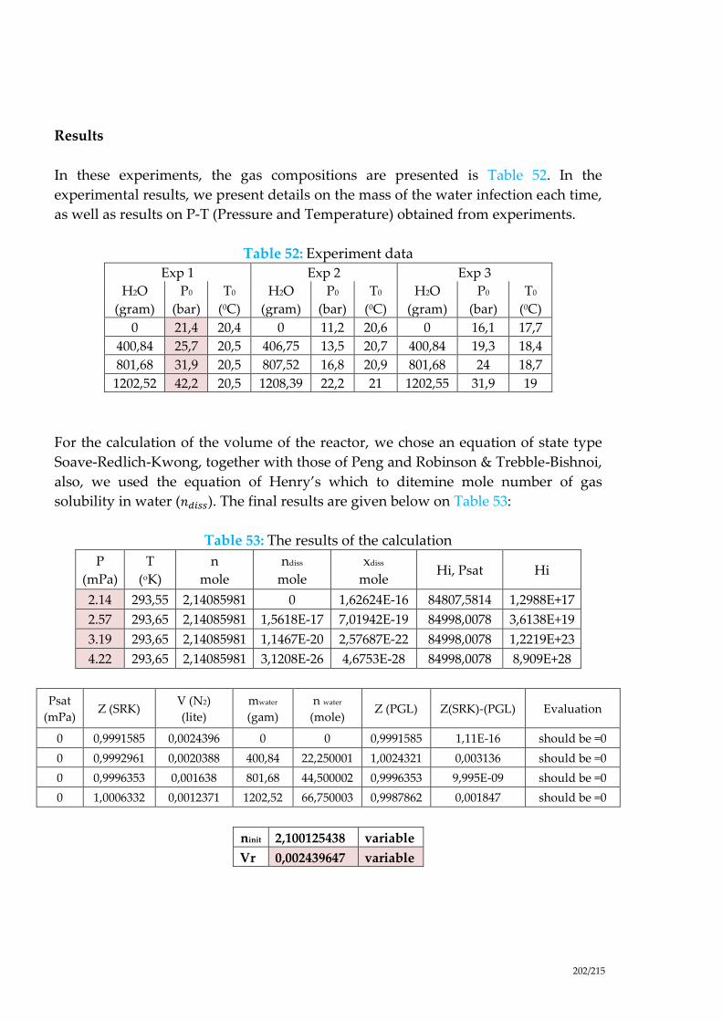
202/215

Results

In these experiments, the gas compositions are presented is Table 52. In the

experimental results, we present details on the mass of the water infection each time,

as well as results on P-T (Pressure and Temperature) obtained from experiments.

Table 52: Experiment data

Exp 1 Exp 2 Exp 3

H2O

(gram)

P0

(bar)

T0

(0C)

H2O

(gram)

P0

(bar)

T0

(0C)

H2O

(gram)

P0

(bar)

T0

(0C)

0 21,4 20,4 0 11,2 20,6 0 16,1 17,7

400,84 25,7 20,5 406,75 13,5 20,7 400,84 19,3 18,4

801,68 31,9 20,5 807,52 16,8 20,9 801,68 24 18,7

1202,52 42,2 20,5 1208,39 22,2 21 1202,55 31,9 19

For the calculation of the volume of the reactor, we chose an equation of state type

Soave-Redlich-Kwong, together with those of Peng and Robinson & Trebble-Bishnoi,

also, we used the equation of Henry’s which to ditemine mole number of gas

solubility in water (𝑛𝑑𝑖𝑠𝑠). The final results are given below on Table 53:

Table 53: The results of the calculation

P

(mPa)

T

(oK)

n

mole

ndiss

mole

xdiss

mole Hi, Psat Hi

2.14 293,55 2,14085981 0 1,62624E-16 84807,5814 1,2988E+17

2.57 293,65 2,14085981 1,5618E-17 7,01942E-19 84998,0078 3,6138E+19

3.19 293,65 2,14085981 1,1467E-20 2,57687E-22 84998,0078 1,2219E+23

4.22 293,65 2,14085981 3,1208E-26 4,6753E-28 84998,0078 8,909E+28

Psat

(mPa) Z (SRK)

V (N2)

(lite)

mwater

(gam)

n water

(mole) Z (PGL) Z(SRK)-(PGL) Evaluation

0 0,9991585 0,0024396 0 0 0,9991585 1,11E-16 should be =0

0 0,9992961 0,0020388 400,84 22,250001 1,0024321 0,003136 should be =0

0 0,9996353 0,001638 801,68 44,500002 0,9996353 9,995E-09 should be =0

0 1,0006332 0,0012371 1202,52 66,750003 0,9987862 0,001847 should be =0

ninit 2,100125438 variable

Vr 0,002439647 variable

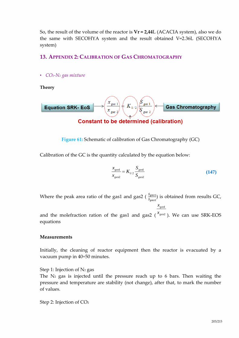
203/215

So, the result of the volume of the reactor is Vr = 2,44L (ACACIA system), also we do

the same with SECOHYA system and the result obtained V=2.36L (SECOHYA

system)

13. APPENDIX 2: CALIBRATION OF GAS CHROMATOGRAPHY

• CO2-N2 gas mixture

Theory

Figure 61: Schematic of calibration of Gas Chromatography (GC)

Calibration of the GC is the quantity calculated by the equation below:

2

1

2/1

2

1

gas

gas

gas

gas

S

SK

x

x

(147)

Where the peak area ratio of the gas1 and gas2 ( 𝑆𝑔𝑎𝑠1

𝑆𝑔𝑎𝑠2) is obtained from results GC,

and the molefraction ration of the gas1 and gas2 ( 2

1

gas

gas

x

x

). We can use SRK-EOS

equations

Measurements

Initially, the cleaning of reactor equipment then the reactor is evacuated by a

vacuum pump in 40÷50 minutes.

Step 1: Injection of N2 gas

The N2 gas is injected until the pressure reach up to 6 bars. Then waiting the


of values.

Step 2: Injection of CO2

204/215

The stirrer is stopped; the second gas, CO2 is injected into reactor. Then waiting the


of values.

Step 3: Injection of CO2

Do the same step 2

The Experimental is slooped sevaral times until the pressure reach up to 40÷45 bars.

(See Table 54)

Table 54: Experiment results

Exp

no

P

(bar)

T

(0C) SN2 SCO2

N2 6,2 5,2 12111,6 0

1

11,2 5,15 11344,6 11153,6

16,1 5,35 11722,3 23561,3

20,6 5,5 11469,9 35082,1

25,6 5,45 11051,5 47588,8

30,5 5,5 11245 63922,6

35,2 5,5 10799 77865,1

40,5 5,2 10376,6 95846,3

44,3 5,05 9711,9 105058,5

N2 4,2 5,8 8668,9 0

2

7,5 5,65 9285,9 8565,2

11,4 5,75 8359,5 17252,9

15,1 5,8 8360,1 27056,5

18,9 5,8 8894,5 40029,9

22,8 5,8 8490,9 50334,7

26,7 5,25 8377,5 62451

30,7 5,2 8749,8 80312,5

34,7 5,2 7938,7 87747,4

38,6 5,2 8289,3 108756,1

CO2 6,6 5,35 0 15124,9

3

11,2 5,35 10037 16984

16 5,5 21049,7 17262,8

21,4 5,2 35714 18907,2

28,1 5,2 52678,2 19186,3

36,5 5,3 81148,1 21263,3

40,7 5,25 93885,8 21568,3

46 5,3 112882,3 22608,3

CO2 4,1 5,05 0 5991,5

4 8 5,1 6311 7482,9

13,2 5,25 14896,7 7761,8

205/215

17,1 5,3 21962 8078,6

20,6 5,35 28925,6 8392,9

23,4 5 44691,5 11166,6

26,7 5,05 54963,1 11753,1

29,4 5,15 67052,8 12776,6

32,1 5,15 80049 13789,2

34,3 5,15 89183 14203,2

37 5,25 86014,3 12595,5

39,7 5,25 102246,2 13836,6

41,6 5,25 108124,7 13892,8

44,2 5,25 123596,9 14936,4

46,4 5 118037,9 13642,5

Results

Figure 62: Calibration curve of gas chromatograph of CO2-N2 gas mixture

The result is given certainty between the point on curve (y = 1.1731x – 0.0138)

compare with in fact is 3.2%.

Do the same method with other gas mixtures in our experiments.

y = 1,1731x - 0,0138R² = 0,9999

0

3

6

9

0 3 6 9

XN

2/X

CO

2

SN2/SCO2

Calibration N2/CO2

Linéaire (CalibrationN2/CO2)

206/215

• CH4-C3H8 gas mixture

Figure 63: Calibration curve of gas chromatograph of CH3-C3H8 gas mixture

• CO2-CH4 gas mixture

y = 0,385x + 0,001R² = 0,990

0

0,01

0,02

0,03

0,04

0,05

0,06

0,07

0,08

0,09

0 0,05 0,1 0,15 0,2 0,25

XC

3H

6/X

CH

4

SC3H6/SCH4

C3/C1

y = 0.6902xR² = 0.999

0.00

1.00

2.00

3.00

4.00

5.00

6.00

0.00 1.00 2.00 3.00 4.00 5.00 6.00 7.00 8.00

XC

O2

/XC

H4

SCO2/SCH4

207/215

Figure 64: Calibration curve of the gas chromatograph for CO2-CH4

• C2H6-C3H8 gas mixture

Figure 65: Calibration curve of the gas chromatograph for C2H6-CH4

y = 0,678x - 0,000R² = 0,995

0

0,05

0,1

0,15

0,2

0,25

0 0,05 0,1 0,15 0,2 0,25 0,3 0,35

X(C

2H

6)/

X(C

H4

)

S(C2H6)/S(CH4)

C2/C1

208/215

209/215

14. APPENDIX 3: EVALUATION OF ERRORS CALCULATION

• Evaluation of the initial quantity of gases in the reactor from pressure balance.

The principle of the preparation of the gases is to generate a binary mixture (for

example CO2 and N2) with a given molar composition (y(A) and y(B)) by the

following procedure:

0- Temperature is controlled to T value

1- After vacuuming, a volume V of reactor (temperature T), inject the first gas

(A) into the reactor up to a pressure P1

2- Inject second gas (B) to a pressure P2

3- Back calculate the molar composition nA, nA+B and nB = nA+B-nA by using

the following algorithm (Figure 66)

Figure 66: Algorithm of calculation on the molar composition

210/215

Calculation of error

After convergence, the gas composition is calculated from

RTZ

VPn

PA

A

1

1

RTZ

VPnn

PBA

G

BA

2

2

A

PBA

B nRTZ

VPn

2

2

(148)

So, a direct evaluation of error on An and BAn gives

T

T

Z

Z

V

V

P

P

n

n

PA

PA

A

A

1

1

1

1

(149)

and

T

T

Z

Z

V

V

P

P

n

n

PBA

PBA

BA

BA

1

2

2

2

(150)

So finally

A

A

BA

BA

B

B

n

n

By

Ay

n

n

Byn

n

1

(151)

The error on evaluation of pressure is ∆P = 0.01mPa

The error on evaluation of reactor is volume ∆V = 0.001lite

The error on the valuation of compressibility factor is not evaluated here, and

considered as negligible compared to other

The error on temperature is T= 0.02 oK

In regard to the precision of the instrument, the error is mainly due to the precision

in the evaluation of the pressure:

1

1

P

P

n

n

A

A

and 2

2

P

P

n

n

BA

BA

and A

A

BA

BA

B

B

P

P

By

Ay

P

P

Byn

n

1

(152)

211/215

• Evaluation of the error on Ay and By from gas chromatography

After sampling of the gas phase, once

BS

AS

has been determined by gas

chromatography, the value of

By

Ay

is determined from the previous calibration

curve:

By

Aya

and 1 ByAy ; so

a

aAy

aAy

111

and

a

aAy

1 (153)

So, the error on the evaluation of Ay (or By ) is

a

a

By

By

Ay

Ay

2

(154)

and value of 2%

• Evaluation of the error G

jerr of the mole number of gas in the gas phase at time t.

At time t, the composition of the gas is given form gas chromatography ( yy =0.02)

and pressure measurement (P=0.01mPa).

TRypTZ

VPn

j ),,(

RG

and jj ynn GG

(155)

j

j

j

j

y

y

n

n

n

n

G

G

G

G

and P

P

n

nG

G

(156)

With P=0.01mPa and y/y = 0.02, we obtain an estimation of the error that is

always superior to 2%, inferior to 3% as soon as the pressure is superior to 0.5 mPa ,

and inferior to 2.5% as soon as the pressure is superior to 1 MPa. In our experiments,

pressure is always superior to 1 MPa, and we will retain that

𝑒𝑟𝑟𝑗𝐺 =

∆𝑛𝑗𝐺

𝑛𝑗𝐺 = 0.025 (157)

212/215

• Evaluation of the error on the calculation of the gas mole number consumption between

two steps at phase at time t1 and t2

We evaluate the error on the calculation of GG

0 jj nn that is the quantity of gas that has

been transferred to solution, i.e. dissolution and crystallisation.

jj

jj

jj yTRyPTZ

VPy

TRyPTZ

VPnn

),,(),,(

R

000

R0GG0

(158)

In a good approximation, we can write

jjjj yPyP

TRZ

Vnn 00

RGG0

(159)

with

2

),,(),,( 00 jj yPTZyPTZZ

(160)

Secondly, in consideration that the evaluation of the mole number is first order

depend on the precision of pressure P and composition z, we can write:

jjjjjj dyPydPdyPydP

TRZ

Vnnd 0000

RGG0

(161)

So

yPPyyP

TRZ

Vnn jjjj 000

RGG0

(162)

∆൫𝑛𝑗0

𝐺 − 𝑛𝑗𝐺൯

𝑛𝑗0𝐺 − 𝑛𝑗

𝐺 < (2∆𝑃0

𝑃0+ 2(∆𝑦)) < 5% (163)

The same calculation can be done for the total amount of gas:

0

0

GG

0

GG

02

P

P

nn

nn

(164)

213/215

• Evaluation of the error L

jerr of the mole number of gas in the liquid phase at time t

Gas composition of the liquid phase is determined from a Henry correlation (see in

the mole number of gas in the liquid phase at method calculation of mass balance).

RTPvK

Py

M

Vn

jj

jj

j

exp,H

G

w

w

L

L

(165)

In a first approximation, we can write that:

P

P

K

K

V

V

n

n

j

j

j

j

,H

,H

L

L

L

L

(166)

With

]Li[

]Li[ 0

L

0L

V

V

(167)

and so

]Li[

]Li[

]Li[

]Li[

0

0

L

0

L

0

L

L

V

V

V

V

(168)

∆𝑉0

𝐿

𝑉0𝐿 ≪ 0.001 because it is determined from mass measurement, with precision of

0.01g and total mass of water around 1 kg.

∆[𝐿𝑖+]

[𝐿𝑖+]≪ 0.001 in reason of the precision of the ionic chromatography

So, we can give an evaluation of

P

P

K

K

n

n

j

j

j

j

,H

,H

L

L

(169)

214/215

Without an evaluation of the precision of the Henry constant, we will overestimate it

to 10%, so that 𝑒𝑟𝑟𝑗𝐿 =

∆𝑛𝑗𝐿

𝑛𝑗𝐿 ≈ 0.1. We will see after there is no consequence on the

evaluation of the mole number of gas in the hydrate phase (see following) because of

low quantity of gas in the liquid phase in respect to the quantity in the gas phase and

hydrate phase;

• Evaluation of error of the mole number of gas in the hydrate phase.

The mole number of gas in the hydrate phase is calculated from a mass balance from

Eq. (115)

0,

GLH jjjj nnnn

(170)

In a first approximation, because of the very low solubility of gases in water, we

have also

H

jj nn L

and 0,

GH jjj nnn

(171)

So, from Eq. (163) we obtain

∆𝑛𝑗

𝐻

𝑛𝑗𝐻 ≈

∆൫𝑛𝑗𝐺 − 𝑛𝑗,0൯

𝑛𝑗𝐺 − 𝑛𝑗,0

< 5% (172)

• Evaluation of the error on the calculation of composition (molar fraction) of gas in the

hydrate

In a first approximation that assumes the quantity of gas in liquid is negligible

compared to other quantities (hydrate and gas phases), we can write:

GG

0

H

H

H

nn

n

n

nx

j

i

i

jH

j

(173)

and

GG

0

H

2GG

0

GG

0

H1

nndnnnnn

dndx j

jH

j

(174)

215/215

that gives

GG

0

GG

0

GG

0

H

GG

0

H

nn

nn

nn

n

nn

nx

jjH

j

(175)

with Eq. (163)

0

0

GG

0

GG

02

P

P

nn

nn

(176)

we get

01.005.0

H

H

j

H

H

jH

jn

n

n

nx

(177)

So, finally, the evaluation is:

06.0

H

j

H

j

x

x

(178)

École Nationale Supérieure des Mines

de Saint-Étienne

NNT: 2016LYSEM002

Quang-Du LE

INVESTIGATION OF NON-EQUILIBRIUM CRYSTALLIZATION OF MIXED

GAS CLATHRATES HYDRATES: AN EXPERIMENTAL STUDY

COMPARED TO THERMODYNAMIC MODELING WITH AND WITHOUT

FLASH CALCULATIONS

Speciality: Process engineering

Keywords: Gas Hydrates, Thermodynamic, Kinetic, Crystallization, CO2 capture and storage,

Flow assurance, Phase equilibria, Flash calculations

Abstract:

The scientific goal of this thesis is based on the acquisition of experimental data and the modeling of the

composition of clathrates gas hydrate. The domains of application concern the gas separation and storage,

water purification, and energy storage using change phase materials (PCMs).

Our research team has recently demonstrated that the composition of gas hydrates was sensitive to the

crystallization conditions, and that the phenomenon of formation was out of thermodynamic equilibrium.

During this thesis, we have investigated several types of crystallization, which are based on the same

initial states. The goal is to point out the differences between the initial solution composition and the final

solution composition, and to establish a link between the final state and the crystallization rate.

Depending on the rate of crystallization (slow or fast), the acquisition time of experimental data lasted

from a few days to several weeks. The experimental tests were performed inside a stirred batch reactor

(autoclave, 2.44 or 2.36 L) cooled with a double jacket. Real-time measurements of the composition of

the gas and the liquid phases have been performed, in order to calculate the composition of the hydrate

phase using mass balance calculations. Depending on the crystallization mode, we have identified several

variations of the composition of the hydrate phase and final hydrate volume.

We have established a successful thermodynamic model, which indicates the composition of the hydrate

phase and hydrate volume in thermodynamic equilibrium state using a gas mixture which had never been

used before in the literature. So this thermodynamic model has required an extremely slow experimental

test. These tests were also long in order to be sure of the thermodynamic equilibrium state.

We are currently establishing a kinetics model in order to model the deviations from the reference point

of equilibrium of our experimental tests which were carried out at a high crystallization rate.

École Nationale Supérieure des Mines

de Saint-Étienne

NNT: 2016LYSEM002

Quang-Du LE

INVESTIGATION DE LA CRISTALLISATION HORS-ÉQUILIBRE DES

CLATHRATES HYDRATES DE GAZ MIXTES: UNE ÉTUDE

EXPÉRIMENTALE COMPARÉE À LA MODÉLISATION

THERMODYNAMIQUE AVEC ET SANS CALCULS FLASH

Spécialité: Génie des Procédés

Mots clefs: Clathrate hydrates, Captage et Stockage du CO2, Thermodynamique, Cinétique,

Cristallisation, Flow assurance, Phase équilibrais, Calculs flash.

Résumé :

L’activité scientifique du sujet porte sur l’acquisition de données expérimentales et la modélisation

de la composition des clathrates hydrates de gaz. Les domaines d’application concernent la

séparation et le stockage de gaz, la purification de l’eau, et le stockage d’énergie par matériaux à

changement de phase.

L’équipe a mis en évidence il y a quelques années que la composition des hydrates de gaz était

sensible aux conditions de cristallisation, et que le phénomène de formation se produisait en dehors

de l’équilibre thermodynamique.

Le travail de thèse a permis d’explorer plusieurs modes de cristallisation à partir de solutions de

même composition initiale pour observer les différences concernant l’état final, compositions

notamment, et les relier à la vitesse de cristallisation.

Suivant le mode de cristallisation, lent ou rapide, l’acquisition des données expérimentales peut

prendre de quelques jours à plusieurs semaines. Les expériences sont réalisées en réacteur pressurisé

dans lequel nous mesurons en ligne la composition de la phase gaz et de la phase liquide, pour

calculer par bilan de matière la composition de la phase hydrate.

Nous avons bien mis en évidence des variations dans la composition de la phase hydrate suivant le

mode de cristallisation. Nous avons dû établir un modèle thermodynamique donnant la composition

de la phase hydrate à l’équilibre pour des mélanges de gaz qui n’avaient jamais été traité par la

littérature, et qui ont donc nécessité des campagnes de mesure extrêmement lentes et donc longues

pour être sûr de l’état thermodynamique à l’équilibre.

Nous sommes en cours d’établir un modèle cinétique pour modéliser les écarts à cet état d’équilibre

de référence pour nos expériences réalisées à vitesse de cristallisation rapide.

Investigation of non-equilibrium crystallization of mixed gas ...

Documents

Transcript of Investigation of non-equilibrium crystallization of mixed gas ...