Inverse Problems Related toCrystallization of PolymersMartin Burger Vincenzo Capasso� Heinz W.EnglJuly 10, 2000Industrial Mathematics Institute, Johannes Kepler Universit�at Linz,Altenbergerstr. 69, A-4040 Linz, Austria.� on leave from (permanent address):Dipartimento di Matematica, Universit�a di Milano,Via Saldini 50, I-20133 Milano, Italy.AbstractThis paper is devoted to identi�cation problems in polymer crystallization pro-cesses. As a �rst step the identi�cation of nucleation and growth rates from boundarymeasurements will be discussed in the case of one-dimensional crystallization. Thisleads to an identi�cation problem in a coupled system of a hyperbolic and a parabolicequation.An algorithm for the solution of this inverse problem will be developed usingLandweber iteration as a regularization method. The behaviour of the algorithmwill be studied both numerically and mathematically on the basis of the recently de-veloped convergence theory for iterative regularization methods for nonlinear inverseproblems.1 IntroductionMathematical modelling has been very successfully applied to predicting (and eventuallyoptimizing) the �nal morphology of crystallized polymers under various operating condi-tions (cf. e.g. [2, 11, 12, 20, 22]). The quality of the predictions made by mathematicalmodels depends crucially on the use of accurate values for the various physical parametersthat appear in the model. Many of these parameters are not accessible to direct mea-surements and have thus to be determined by 'indirect measurements', i.e., by parameteridenti�cation techniques. As a general reference for parameter identi�cation we refer to[3]. Since parameter identi�cation is an ill-posed inverse problem, major numerical di�cul-ties arise due to the inherent instability of such problems (see [13] for general background1

material on inverse problems and regularization methods for their solution). This issue isespecially important due to the fact that the available measurements are rather noisy.Our aim in this paper is to construct a stable algorithm for identifying temperature-dependent growth and nucleation rates in a recently developed model for one-dimensionalcrystallization (cf.[6]). This algorithm is based on Landweber iteration; for this method,applied to nonlinear inverse problems, a comprehensive convergence theory is available(cf.[10, 18]). We apply this theory to our model in a formal way, i.e., we do not verifycertain theoretical conditions like e.g. the existence of solutions for the direct problem incertain Hilbert spaces, since this would be technically rather involved and would obscurethe basic ideas. Of course, for a complete justi�cation of our method, this will eventuallyhave to be done in future work.The model for one-dimensional crystallization of polymers developed in [6] leads toinitial-boundary value problems of the form@T@t = D@2T@x2 + L@�@t (1.1)@@t 1eG(T )(1� �) @�@t! = @@x eG(T )1� � @�@x!+ 2 @@t( eN(T )) (1.2)with initial conditions T (x; 0) = T 0(x) (1.3)�(x; 0) = 0 (1.4)@�@t (x; 0) = 0 (1.5)and boundary conditions@T@n (x; t) = �(T (x; t)� T 1(x; t)) for x 2 @ (1.6)@�@t (x; t) + eG(T )@�@n(x; t) = 0 for x 2 @; (1.7)where T 1 in (1.6) represents an exterior temperature in the cooling process at the boundary.In these equations, T denotes the temperature, � the degree of crystallinity. Theparameter arising in the heat transfer problem, i.e., the di�usion coe�cient D, the latentheat L and the heat transition coe�cient �, can be determined experimentally. Thefunction eN represents an equivalent nucleation rate per unit of length (cf.[6]) and eG theradial growth rate of a nucleus. Note that eG and eN depend on temperature rather stronglyand cannot (at least not simultaneously) be measured as functions of temperature. Somematerials admit experimental determination of the growth rate (cf.[22]), in these cases theidenti�cation of eN for known eG is of special interest.The measurable quantities in usual experiments are the temperature T on the boundaryof the crystallization domain (or at least on a part of the boundary � � @) as well as2

the degree of crystallinity �(x; t�) at the end of the process. The temperature at the endof the experiment is not measurable, because the structure is frozen in by a �nal quenchbelow the melting point.Furthermore, data about the �nal morphology, i.e., about the �nal distribution of nuclei�(x; t�), are sometimes available, this quantity being linked to the nucleation rate via�(x; t�) = t�Z0 (1� �(x; t))@ eN(T )@t dt: (1.8)The use of such data is di�erent from the use of boundary data and will be discussed inSection 2.4.A major di�erence to parameter estimation problems in parabolic and hyperbolic dif-ferential equations with overspeci�ed boundary data (cf. e.g. [7, 15, 19, 21]) is the strongcoupling of the parabolic and the hyperbolic equation. The fact that the parameter eNand eG are functions of the temperature, but arise in the hyperbolic equation, is anotherunusual feature of this identi�cation problem.1.1 Simpli�cation and ScalingSystem (1.1), (1.2) may be transformed into a system of PDEs of �rst order in time givenby @T@t = D@2T@x2 + L@�@t (1.9)@�@t = (1� �) eG(T )w (1.10)@w@t = @@x eG(T )1� � @�@x!+ 2@ eN(T )@t (1.11)In practical applications the crystallization is performed under symmetric conditions,so that it is reasonable to assume symmetric boundary and initial conditions in the one-dimensional domain = (a; b). Also by symmetry we may restrict the problem to (a; a+b2 )and use the conditions @T@x �a+ b2 ; :� = 0@�@x �a+ b2 ; :� = 0at the new right boundary. 3

By using the quantity v = � ln(1� �), mapping [a; a+b2 ] to [0; 1] and further scaling thesystem may be transformed into the formut = Duxx + Le�vvtvt = a(u)wwt = (a(u)vx)x + b(u)t (1.12)ujt=0 = u0vjt=0 = 0wjt=0 = 0 (1.13)ux(0; t) = ��(u(0; t)� u1(0; t))w(0; t)� vx(0; t) = 0 (1.14)ux(1; t) = 0vx(1; t) = 0: (1.15)The quantities a(u) and b(u) in (1.12) are the equivalents to eG(u) and eN(u), transformedto the new reference variable u. The function u is a scaled temperature, i.e., u = 1 is abovethe equilibrium melting point and u = 0 below the glass transition temperature, hence thetemperature range of interest [u1; u2] is a subset of [0; 1]. In practice, the temperature atthe beginning of the experiment is always above the melting point, i.e., u2 may be chosenas the melting point. The fact that no nucleation occurs above this temperature impliesthat b(u) = 0 for u � u2, so we will restrict our attention to functions b 2 H1([u1; u2])satisfying b(u2) = 0.In the following we will assume that the temperature data are given at the point x = 0by u(0; t) = uB(t) in the time interval I = (0; t�). From the available observation of � att = t� we can compute the value v� for vjt=t�, which we therefore assume to be given.By the remarks made above, identi�cation of the nucleation rate eN = eN(T ) in (1.1)-(1.7) is equivalent to identifying b = b(u) in (1.12)-(1.15). Thus, this identi�cation problemcan formally be written as the nonlinear operator equationF (b) = (u�B; v��); (1.16)where u�B and v�� denote noisy measurements of uB and v� with noise level �. The operatorF , the 'parameter-to-output-map', maps an admissible value of the parameter b to thevalues uB and v� obtained from solving (1.12)-(1.15) with this parameter. In the nextsection we treat the nonlinear operator equation (1.16) in a more formal way and developa stable algorithm for its solution.2 Identi�cation of Nucleation RatesWe assume that for 'admissible' parameter b 2 D(F ) the direct problem (1.12) - (1.15)admits a unique strong solution(u; v; w) 2 X := H1;2(Q)�H2;2(Q)�H1;0(Q);4

which depends continuously on b in theH1-norm, where the time-space domainQ is de�nedby Q := � I = (0; 1)� (0; t�):This well-posedness requirement can also be thought of as an implicit de�nition ofD(F ). Finding conditions on b that guarantee the well-posedness of the nonlinear system(1.12) - (1.15) is in principle standard, but technically quite involved. Under this well-posedness assumption, the operator used in (1.16) can be formally de�ned as a continuousoperatorF : D(F ) � V := f b j b 2 H1([u1; u2]); b(u2) = 0 g ! L2(I)� L2()b 7! (ujx=0; vjt=t�): (2.1)The inverse problem of solving (1.16) is most likely ill-posed, so that regularization hasto be used. One classical possibility would be Tikhonov regularization, i.e., taking asregularized solution (global) minimizers of the functionalb 7! kF (b)� (u�B; v��))kL2(I)�L2() + �kbkH1([u1;u2]) (2.2)over D(F ), where � > 0 is a regularization parameter. The convergence theory for thismethod (for nonlinear problems) has been developed in [14] (cf. also [13]). A major disad-vantage, however, is that since the functional in (2.2) is in general not convex and mighthave many local minima, minimizing (2.2) is not an easy task. Therefore, iterative regu-larization methods are an attractive alternative especially for nonlinear ill-posed problems;the regularization e�ect comes from stopping the iteration at an appropriately de�nedstopping index which depends also on the noise level � ('stopping rule'). The convergencetheory of iterative methods for solving nonlinear ill-posed problems is still a developing�eld of research (see [10, 13, 16] and the references quoted there).Here we use one of the simplest iterative regularization methods, namely Landweberiteration, which nevertheless turned out to be quite e�ective for certain (especially severely)ill-posed nonlinear problems (cf.[17]). In later work we will also investigate the e�ciencyof using Newton-like methods like the iteratively regularized Gau�-Newton method (cf.[5,10]), which is of course faster than Landweber for data without noise, but also ampli�esdata noise faster.For our problem (1.16), Landweber iteration is de�ned bybk+1 = bk � !F 0(bk)�(F (bk)� (u�B; v��)): (2.3)For computing the iterates, the adjoint F 0(bk)� is needed. As we will see later, theadjoint also plays a crucial role in the analysis of the convergence rate. Hence, it isnecessary to be able to compute these adjoints e�ciently. Note that the adjoint dependson the Hilbert spaces between which F acts, so that also the choice of these spaces isimportant. In the following we derive a method of computing the adjoint of F 0 by solvinga system of linear partial di�erential equations. We �rst split F into F = � �, where� : D(F ) � H1([u1; u2]) ! Xb 7! (u; v; w)5

is the parameter-to-solution map and : �(D(F )) � X ! L2(I)� L2()(u; v; w) 7! (ujx=0; vjt=t�)is the trace operator that maps the solution onto u at x = 0 and v at t = t�. As is alinear and continuous operator, the Fr�echet derivative of F is F 0 = ��0. We assume that�0 exists as a Fr�echet derivative (verifying this under appropriate smoothness conditionson a and b would certainly be possible, but quite technical) and proceed in a formal way:By straightforward linearization we conclude that the derivative (U; V;W ) := �0(b)hsatis�es the systemUt = DUxx + Le�v(vtV + Vt)Vt = a(u)W + a0(u)UwWt = (a(u)Vx)x + (a0(u)Uvx)x + (b0(u)U)t + h(u)t (2.4)with initial and boundary conditions given by�U + Ux = 0W � Vx = 0 � for x = 0 (2.5)Ux = 0Vx = 0 � for x = 1 (2.6)U jt=0 = 0V jt=0 = 0W jt=0 = 0: (2.7)System (2.4)-(2.7) is linear in (U; V;W ), but depends on the current value of b and henceon the solution (u; v; w) = �(b) of the nonlinear system (1.12)-(1.15). We again assumethat the solution of (2.4)-(2.7) exists and is unique. From this system, we can computethe derivative of F as F 0(b)h = � �0(b)h: (2.8)2.1 The adjoint problemFor the computation of the adjoint we split F 0(b) asF 0(b)h = S �R � Jh; (2.9)where J is the embedding operator from V onto L2([u1; u2]), R the operatorR : D(F ) � L2([u1; u2]) ! L2(� I)h(u) 7! h(x; t) := h(u(x; t))6

and S is the operator de�ned byS : L2(� I)� L2(I) ! L2(I)� L2()h 7! (U jx=0; V jt=t�);by which we mean the trace of the solution of (2.4)-(2.7) with h(u)t replaced by @h@t (x; t)in the last equation and b being the argument in F 0(b).Because of (2.9), F 0(b)� = J� �R� � S�: (2.10)We compute these three adjoints step by step, starting with S�; this will involve thefollowing problem: �t = �D�xx � a0(u) w � a(u)b0(u) + a0(u)vx�x t = Le�v�t � (a(u)�x)x�t = �a(u) (2.11)�jt=t� = 0 jt=t� = r�jt=t� = 0 (2.12)D��+D�x � a0(u)vx� = q � �x = 0 � at x = 0 (2.13)�x = 0�x = 0 � at x = 1; (2.14)considered as an equation for (�; ; �); note that via u and v, the coe�cients in this systemdepend on b. Again we assume (proceeding still in a merely formal way) unique solvabilityof (2.11)-(2.14).Now let (�; ; �) be the solution of (2.11)-(2.14); in (2.3), (q; r) will be the residual(q; r) = F (b)� (u�B; v��); (2.15)but the argument holds for any (q; r) 2 L2(I)� L2().Integration by parts yieldst�Z0 1Z0 h a(u) dxdt = � t�Z0 1Z0 h �t dxdt= t�Z0 1Z0 ht � dxdt� 1Z0 (h �)jt=t�t=0 dx:7

The assumptions h(x; 0) = h(u(x; 0)) = h(u0(x)) = 0 and �jt=t� = 0 cause the secondintegral to vanish. Using system (2.4) we conclude thatt�Z0 1Z0 ht� dxdt = t�Z0 1Z0 (Wt � (a(u)Vx)x � (a0(u)Uvx)x � (b0(u)U)t) � dxdt;0 = t�Z0 1Z0 �Ut �DUxx � Le�v(vtV + Vt)�� dxdt;0 = t�Z0 1Z0 (Vt � a(u)W � a0(u)Uw) dxdt:By adding these equations and integrating by parts we �nally deducet�Z0 1Z0 h(x; t)a(u(x; t)) (x; t) dxdt = t�Z0 1Z0 ht(x; t)�(x; t) dxdt= 1Z0 U(0; t)q(t) dx+ t�Z0 V (x; t�)r(x) dt;hence S�(q; r) = a(u) ; (2.16)where is de�ned via (2.11)-(2.14).The adjoint of J can be computed by solving��00(u) + �(u) = �(u) (2.17)�0(u1) = 0; �(u2) = 0:; (2.18)for � = J��: The unique solution � satis�es � 2 V and, for any b 2 V ,(b; �)V = (b; �)H1 = u2Zu1 (b0(u)�0(u) + b(u)�(u))du= u2Zu1 (b(u)�(u)) du= (Jb; �)L2 :The computation of the adjoint of R is more involved, so that we will only consider thecase of decreasing temperature, which is the only one of practical interest. If u(x; :) 2 C1(I)8

and ut � c < 0 there exists a regular 'change-of-variables' transformation p : (t; x) 7! (u; x).Because of j det p0(x; t)j = �ut(x; t) and u(p�1(u; x)) = u, the substitution rule for integralsimplies in this case thatt�Z0 1Z0 (Rh)(x; t)'(x; t) dxdt = t�Z0 1Z0 h(u(x; t))'(x; t) dxdt= � u2Zu1 ZI(u) h(u)'(p�1(u; x)) 1ut(p�1(u; x))dx du= u2Zu1 h(u)�� ZI(u) '(p�1(u; x))ut(p�1(u; x))dx� du;where I(u) = f x 2 j 9 t : u(x; t) = u g:Thus, R�' is given by (R�') (u) = � ZI(u) '(p�1(u; x))ut(p�1(u; x)) dx: (2.19)As a straightforward calculation shows, R�' is still well-de�ned in L2([u1; u2]), if u is anelement of H1;2( � I) satisfying ut � c < 0 almost everywhere, by a density argumentthe form (2.19) holds for such u, too. We do not go into details, since (2.19) is not directlyusable numerically anyway.2.2 An Identi�cation AlgorithmSince (2.19) seems not to be usable in a direct way, we compute J�R�' approximately bya projection method: J�R�' satis�es(RJp; ') = [p; J�R�']for all p 2 H1([u1; u2]), where (:; :) is the inner product in L2(Q) and [:; :] the one inH1([u1; u2]). If we choose a �nite-dimensional subspace VN of H1([u1; u2]) with basisfp1; : : : ; pNg, the orthogonal projection ~'N of ~' := J�R�' onto VN may be written as~'N = NXi=1 �ipiand satis�es (RJpi; ') = [pi; ~'] = [pi; ~'N ] = NXj=1 �j[pi; pj];9

so we obtain the linear system P� = �for the coe�cients � = (�1; : : : ; �N), whereP = ([pi; pj])i;j=1;::: ;N� = ((RJpi; '))i=1;::: ;NThe integrals (Rpi; ') can be computed easily, although even a small support of the func-tions pi does not restrict the domain of integration in general . If the functions pi are theusual linear splinespi(s) = 8>>>>>>><>>>>>>>:

s� si�1si � si�1 if si�1 � s � sisi+1 � ssi+1 � si if si � s � si+10 if s =2 (si�1; si+1)and si = iN , P turns out to is a tridiagonal matrix. Hence the system can be solvede�ciently, a decomposition of P can be computed in a preprocessing step.Now, we summarize our algorithm by putting all pieces, especially the various adjointsinvolved, together:Algorithm 2.1. We start with an initial guess b0, as long as the stopping rule is notsatis�ed, we do the following iteration:� Compute F (bk) by solving the nonlinear initial-boundary value problem (1.12) - (1.15)and evaluating (uB; v�).� Compute the residual (q�; r�) by (2.15).� Compute the adjoint S�(q; r) = a(u) by solving the linear initial-boundary valueproblem (2.11) - (2.14).� Compute F 0(bk)�(q; r) = J�R�a(u) by the projection method just described.� Compute the new iterate bk+1 = bk � !F 0(bk)�(q�; r�) with appropriately chosen !(cf. Section 2.3).As stopping rule, we use the discrepancy principle (cf. Section 2.3.1), i.e. the stoppingindex k� is the �rst index with kF (bk)� (u�B; v��)k � ��;where � is an L2-bound for the noise in our observations.We use some �xed � > 2 in the discrepancy principle, although � should rather bechosen according to (2.26) as explained in detail in the following section; however, theinformation needed to compute � according to this theory is not easily available.10

2.3 Convergence Analysis2.3.1 General TheoryWe summarize the basic convergence theory for Landweber iteration for a nonlinear ill-posed operator equation F (x) = y�; (2.20)between Hilbert spaces X and Y (see [10, 13, 18] for details). The right hand side y�represents a perturbation of the exact data y with error level �, i.e.,ky � y�k � �: (2.21)We assume that the exact data y are attainable and the starting value is su�ciently closeto the solution, i.e. there exists a solution x� of (2.20) with � = 0 in B�(x0).Like in the linear case it is important that the iteration given byx�k+1 = x�k � F 0(x�k)�(F (x�k)� y�) (2.22)is properly scaled, i.e., either kF 0(x)k � 1; 8 x 2 B�(x0); (2.23)or an appropriate damping factor ! is used.Besides existence of a solution for exact data, the following condition is importantfor all convergence proofs (also for other iterative methods for solving nonlinear ill-posedproblems):kF (x)� F (x)� F 0(x)(x� x)k � �kF (x)� F (x)k; 8 x; x 2 B�(x0) � D(F ); (2.24)where � is a real number satisfying � < 12 . It has been shown by Hanke et al. [18] that(2.24) implies the existence and uniqueness of a solution xy of (2.20) of minimal distanceto the starting point x0. For an analysis of this condition, which somehow restricts thenonlinearity of F see [4, 18, 23].Convergence of the Landweber iteration can be shown if the stopping index k� =k�(�; y�) is chosen according to the generalized discrepancy principle (cf.[13, 18])kF (x�k�)� y�k � �� � kF (x�k � y�k; 0 � k < k�; (2.25)where � is a positive real number satisfying� > 2 1 + �1� 2� > 2: (2.26)Convergence rates can, as usual for ill-posed problems even in the linear case, only beestablished if 'source conditions' are satis�ed. If the di�erence between the starting iterateand the true solution satis�esxy � x0 = (F 0(xy)�F 0(xy))�w1; (2.27)11

with 0 < � � 12 , the convergence ratek� � c1�kw1k� � 22�+1 (2.28)kxy � x�k�k � c2kw1k 12�+1 � 2�2�+1 (2.29)can be proved under some additional assumptions (cf.[18]). The stopping index can beestimated by (2.28). In the case of � = 12 , (2.27) is equivalent toxy � x0 = F 0(xy)�w0: (2.30)Thus, the adjoint is also needed for assessing the convergence rate. Under (2.30), theconvergence rate is kxy � x�k�k = O(p�); (2.31)the stopping index can be estimated byk� = O(1� ): (2.32)2.3.2 Application to Our Identi�cation ProblemIn the special case of identifying b in (1.12)-(1.15), the source condition (2.30) can beinterpreted as follows. If ut < 0, i.e., the temperature is decreasing, we may write(R�S�(q; r)) (u) = �a(u) ZI(u) (p�1(u; x))ut(p�1(u; x)) dx; (2.33)where is de�ned by (2.11)-(2.14). Together with the adjoint of the embedding operatorJ one obtains the source conditionby � b0 = J�R�S�(~q; ~r); (2.34)where the last step is to solve (2.17), (2.18) with the special right-hand-side � = R�S�(q; r).A standard regularity argument for the homogenous two-point boundary value problem(2.17), (2.18) implies that its solution � is in H2+�([u1; u2]) if � 2 H�([u1; u2]). From(2.33) we know at least � = R�S�(q; r) 2 L2([u1; u2]), henceby � b0 2 f ' 2 H2([u1; u2]) j '0(u1) = 0; '(u2) = 0 g (2.35)is necessary for (2.34).Since the source condition is needed for getting a fast convergence rate for the identi-�cation problem, one should, if at all possible, try to set up the problem (and the startingiterate) in such a way that it is ful�lled. This leads to the following conclusions:12

� The fact that temperature should decrease during the process (cf. (2.19) and thediscussion below) is heuristically obvious, because one just cannot identify a functionof temperature in an experiment at constant temperature. This property is usuallysatis�ed in experiments using Di�erential Scanning Calorimetry (cf.[11]), but not inthe case of isothermal experiments, which have been used for attempts of parameteridenti�cation with di�erent methods in the past (cf.[1, 8]).� Furthermore, formula (2.34) shows that the values of the nucleation rate at temper-atures that do not occur in the experiment have to be incorporated into the initialguess b0, because R�S�(p; q) is always zero at these values of the temperature, whichis also heuristically clear. The temperature range [T1; T2] occurring in the experimentcan be determined in practice. As the temperature of the material is always con-trolled by cooling at the boundary, it attains its minimum there. The maximum T2is always the melting point of the material, because the experiment must be startedat a sample temperature above the melting point.� The smoothness condition by � b0 2 H2([u1; u2]) in (2.35) means that only smoothparts of by should be computed in the iteration procedure, rougher parts shouldbe incorporated into the initial guess b0 in order to obtain fast convergence. Thecondition at the right boundary in (2.35) can be satis�ed easily, because we haverestricted the domain of F to V using the a-priori knowledge b(u2) = 0. Ful�llingthe condition at the left boundary�by�0 (u1) = �b0�0 (u1); (2.36)is much more di�cult. If u1 represents the glass transition temperature of the mate-rial we may use the a-priori knowledge that the nucleation rate is constant at tem-peratures below, i.e., b0(u) = 0 for u � u1, so we assume b0(u1) = 0 for the solutionand incorporate this boundary condition into the initial guess b0. In experiments,where not the whole temperature range between melting point and glass transitiontemperature may occur, so that u1 is higher than the melting point, we may expecta fast convergence rate only if we know b0(u1), which is a strong, maybe unrealisticassumption.2.4 Data about the MorphologyThe identi�cation of rates from information about the �nal morphology di�ers from theabove identi�cation problem, because (1.8) does not only contain information at the bound-ary or the �nal time, but averaged information in the whole time-space domain. Thisidenti�cation problem could be handled in a similar way, we just give a short sketch of thenecessary ingredients:The parameter-to-data map is given byH : D(H) � H1([u1; u2]) ! L2() (2.37)b 7! �jt=t�; (2.38)13

where �(x; t) = tZ0 e�v(x; �)b(u(x; s))s ds:The derivative H 0(b)h is given by(H 0(b)h) (x) = t�Z0 e�v (�V b(u) + (b0(u)U)t + h(u)t) dt;where (U; V;W ) is the solution of (2.4)-(2.7).Similar to (2.11)-(2.14) we de�ne an adjoint problem by�t = �D�xx � a0(u) w � a(u)b0(u) � a0(u)vx� + e�vvtb0(u)p t = Le�v�t + (a(u)Wx)x + e�vp�t = �a(u) (2.39)�jt=t� = 0 jt=t� = 0�jt=t� = 0 (2.40)D���D�x � a0(u)vx� = b0(1� e�v)p�x + = 0 � at x = 0 (2.41)�x = 0�x = 0 � at x = 1 (2.42)where p represents the residual p = H(b)� ��:Integration by parts yields1Z0 (H 0(b)h) p dx = t�Z0 1Z0 h(u) ��e�vp�t dxdt+ 1Z0 �h(u)e�vp� jt=t� dx: (2.43)By splittingH 0 analogously as in Section 2.1 it is possible to compute the adjointH 0(b)pby �rst solving the linear initial-boundary value problem (2.39) - (2.42) and then computingan adjoint similary to J�R�. The main di�erence is that instead of R the operator~R : D(H) � L2([u1; u2]) ! L2(� I)� L2()h(u) 7! (h(x; t); h�(x)) = (h(u(x; t)); h(u(x; t�))14

0 0.1 0.2 0.3 0.4 0.5 0.6 0.7 0.8 0.9 1−0.2

0

0.2

0.4

0.6

0.8

1

1.2

0 0.1 0.2 0.3 0.4 0.5 0.6 0.7 0.8 0.9 10

0.2

0.4

0.6

0.8

1

1.2

1.4

Figure 1: Exact and perturbed data for the boundary temperature, � = 0:025. The left�gure corresponds to an experiment with temperature values in the whole range [0; 1], theright to an experiment with temperature not decreasing below 0:2.has to be used because of the second integral at the right-hand side of (2.43).The data about the morphology can be used together with measurements of the bound-ary temperature and the �nal degree of crystallinity, in this case the parameter-to-datamap consists of three components, i.e., b is mapped to (uB; ��;��). Because of the dif-ferent structures of boundary or �nal data and the data �� about the morphology it isnot possible to compute the adjoint of the parameter-to-data map needed for the Landwe-ber iteration by solving one initial-value problem. Systems (2.11)-(2.14) and (2.39)-(2.42)must be solved separately to obtain the adjoints of the components, the adjoint of theparameter-to-data map is then just their sum. Although we did not perform numericaltests with this setup of the problem, it seems obvious that additional information aboutthe morphology will improve the quality of the solution.3 Numerical ResultsFor the sake of simplicity we perform �rst numerical experiments for constant a (a = 1,a = 0:5 and a = 0:05), which has technical rather than conceptual reasons. The behaviouris similar to the relevant case of a bounded away from 0 uniformly, i.e. if a positive realnumber a0 exists, such that a(u) � a0; 8 u 2 ([u1; u2]):The 'exact data' are computed by solving the direct problem with a very �ne dis-cretization and then perturbed by adding a high-frequency data error of L2-norm � (withfrequencies f = 30, 50, 100 and an error level between 0:5 and 5%). The perturbed data u�Band v�� are obtained by sampling using a di�erent discretization. We perform two kinds of15

0 0.1 0.2 0.3 0.4 0.5 0.6 0.7 0.8 0.9 10

0.5

1

1.5

2

2.5

3

3.5

0 0.1 0.2 0.3 0.4 0.5 0.6 0.7 0.8 0.9 10

0.5

1

1.5

2

2.5

3

3.5

Figure 2: Exact solution (solid) and iterate at k = k� (dotted) vs. u, � = 0:025, f = 50.The left �gure corresponds to an experiment with temperature values in the whole range[0; 1], the right to an experiment with temperature not decreasing below 0:2 (see Figure1).experiments, the �rst with temperature values in the whole range, i.e., [u1; u2] = [0; 1], andthe second with a relevant temperature range [u1; u2] = [0:2; 1] (see Figure 1). The 'exact'rate b we use is similar to the (rare) measurements made for nucleation rates (cf.[6]).The results for the case [u1; u2] = [0:2; 1] are illustrated at the right hand side of Figure2. In this case, a source condition cannot be satis�ed, because our starting iterate does notsatisfy the boundary condition (2.36), so the convergence may be arbitrary slow. Never-theless, the approximation in the accessible temperature range is acceptable; a comparisonwith the left part of Figure 2, which illustrates the corresponding result for [u1; u2] = [0; 1],shows that the di�erence between exact and approximate solutions is larger only in themissing temperature range [0; 0:2). For all further tests and the numerical con�rmation ofthe predictions made by the theory we consider the case [u1; u2] = [0; 1], with a startingiterate satisfying the source condition (2.30) or at least the necessary condition (2.35).For the discrepancy principle, we use a relatively small parameter � , here � = 2:1. Asin Figure 4, the residual in our computations usually did not decrease signi�cantly belowthe value 2�. The numerical experiments show that the discrepancy principle (2.25) with� = 2:1 yields good results, a comparison of the iterates around the stopping index showsthat the choice of the stopping index is not too critical for a = 0:5 and a = 1. This is dueto the slow convergence speed of Landweber iteration and would probably be more criticalfor Newton-type methods. The choice of the stopping index is more critical in the case ofa 'small' parameter a, which may occur in practice (cf.[6]), in our computations a = 0:05.This demonstrates again the ill-posedness of the problem, as Figure 5 shows, only the �rstfew iterates are close to the solution, a choice of � less than 2 would lead to a high errorbetween approximate and exact solution. Nevertheless, the solution determined using thediscrepancy principle is always close to the iterate with minimal error in the H1-norm,16

0 0.1 0.2 0.3 0.4 0.5 0.6 0.7 0.8 0.9 1−0.5

0

0.5

1

1.5

2

2.5

3

3.5

Figure 3: Exact solution (solid) and iterate at k = k� (dotted) vs. u, � = 0:01, f = 30,a = 1.

0 50 100 150 200 250 300 350 4000

0.05

0.1

0.15

0.2

0.25

0 50 100 150 200 250 3000.04

0.06

0.08

0.1

0.12

0.14

0.16

0.18

0.2

0.22

0.24

Figure 4: Residual (solid) and error kbk � bk vs. iteration number for a = 0:5, � = 0:01(left) and � = 0:025 (right), f = 50. The stopping index is marked by �.17

0 50 100 150 200 250 3000.02

0.04

0.06

0.08

0.1

0.12

0.14

0.16

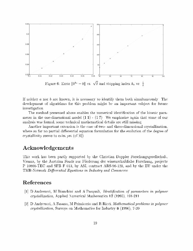
Figure 5: Residual (solid) and error kbk � bk vs. iteration number for a = 0:05, � = 0:02,f = 50. The stopping index is marked by �.which demonstrates again the importance of a good stopping rule.The damping factor ! clearly depends on the size of a, for our choice of the parametera and b the method works without damping, although a line search strategy seems recom-mendable for accelerating the convergence speed. In the case of a = 0:05 we found that theparameter choice ! > 1 leads to higher convergence speed. Nevertheless, one should notuse a high ! if the residual is close to ��, because the faster convergence will also decreasethe number of iterates close to the solution, which makes the choice of a good stoppingindex even more di�cult.As � ! 0, one observes that the approximations bk� converge to the exact solution,which is also illustrated by the results for a noise level of 2:5% at the left hand side ofFigure 2 and for a noise level of 1% in Figure 3. The residual and the di�erence betweenexact and approximate solutions develop as predicted by the theory, especially one observesthat the di�erence to the exact solution tends to zero as p� and the stopping index behavesas 1� (see Figure 6), i.e., (2.31) and (2.32) are con�rmed numerically.4 ExtensionsSimilar to the identi�cation of nucleation rates, growth rates can be determined usingLandweber iteration. The nonlinear operator that maps the parameter onto the data isgiven by G : D(G) � H1([u1; u2]) ! L2(I)� L2() (4.1)a 7! (ujx=0; vjt=t�): (4.2)18

0.1 0.11 0.12 0.13 0.14 0.15 0.160.32

0.34

0.36

0.38

0.4

0.42

40 50 60 70 80 90 1000

50

100

150

200

250

Figure 6: Error kbk� � bk vs. p� and stopping index k� vs. 1� .If neither a nor b are known, it is necessary to identify them both simultaneously. Thedevelopment of algorithms for this problem might be an important subject for futureinvestigation.The method presented above enables the numerical identi�cation of the kinetic para-meter in the one-dimensional model (1.1) - (1.7). We emphasize again that some of ouranalysis was formal, some technical mathematical details are still missing.Another important extension is the case of two- and three-dimensional crystallization,where so far no partial di�erential equation formulation for the evolution of the degree ofcrystallinity seems to exist yet (cf.[6]).AcknowledgementsThis work has been partly supported by the Christian Doppler Forschungsgesellschaft,Vienna, by the Austrian Fonds zur F�orderung der wissenschaftliche Forschung, projectsP 10866-TEC and SFB F 013, by ASI, contract ARS-96-121, and by the EU under theTMR-Network Di�erential Equations in Industry and Commerce.References[1] D.Andreucci, M.Bianchini and A.Pasquali, Identi�cation of parameters in polymercrystallization, Applied Numerical Mathematics 17 (1995), 191-211.[2] D.Andreucci, A.Fasano, M.Primicerio and R.Ricci, Mathematical problems in polymercrystallization, Surveys on Mathematics for Industry 6 (1996), 7-20.19

[3] H.T.Banks, K.Kunisch, Estimation Techniques for Distributed Parameter Systems,(Birkh�auser, Basel, Boston, Berlin,1989).[4] A.Binder, M.Hanke, O.Scherzer, On the Landweber iteration for nonlinear ill-posedproblems, J.Inv.Ill-Posed Problems 4, 381-389 (1996).[5] B.Blaschke, A.Neubauer, O.Scherzer, On convergence rates for the iteratively regular-ized Gauss-Newton method, IMA Journal of Numerical Analysis 17 (1997), 421-436.[6] M.Burger, V.Capasso, G.Eder: Modelling non-isothermal crystallization of polymers,working paper, Industrial Mathematics Institute, University of Linz (1998).[7] J.R.Cannon, P.DuChateau, K.Steube, Unknown ingredients inverse problems andtrace-type functional di�erential equations, in [9], 185-200.[8] V.Capasso, M.DeGiosa, R.Mininni, Asymptotic properties of the maximum likelihoodestimators of parameters of a spatial counting process modelling crystallization of poly-mers, Stoch. Anal. Appl. 13 (1995), 279-294.[9] D.Colton, R.Ewing, W.Rundell (eds.), Inverse Problems in Partial Di�erential Equa-tions (SIAM, Philadelphia, 1990).[10] P.Deu hard, H.Engl, O.Scherzer, A convergence analysis of iterative methods for thesolution of nonlinear ill-posed problems under a�nely invariant conditions, Techni-cal Report 2/1998, Industrial Mathematics Institute, University of Linz (1998), andsubmitted.[11] G.Eder, Fundamentals of structure formation in crystallizing polymers, in K.Hatada,T.Kitayama, O.Vogl, eds., Macromolecular Design of polymeric Materials (M.Dekker,New York, 1997), 761-782.[12] G.Eder, H.Janeschitz-Kriegl, S.Liedauer, Crystallization processes in quiescent andmoving polymer melts under heat transfer conditions, Progr.Polym.Sci. 15:629(1990)[13] H.Engl, M.Hanke and A.Neubauer, Regularization of Inverse Problems (Kluwer, Dor-drecht, 1996).[14] H.Engl, K.Kunisch, A.Neubauer, Convergence rates for Tikhonov regularization ofnonlinear ill-posed problems, Inverse Problems 5 (1989), 523-540.[15] H.Engl, O.Scherzer, M.Yamamoto, Uniqueness and stable determination of forcingterms in linear partial di�erential equations with overspeci�ed boundary data, InverseProblems 10 (1994), 1253-1276.[16] M.Hanke, A regularization Levenberg-Marquardt scheme, with applications to inversegroundwater �ltration problems, Inverse Problems 13 (1997), 79-95.20

[17] M.Hanke, F.Hettlich, O.Scherzer, The Landweber iteration for an inverse scatteringproblem, in K.W.Wang (ed.), Proceedings of the 1995 Design Engineering Techni-cal Conference, Vol.3, Part C, Vibration, Control, Analysis and Identi�cation, TheAmerican Society of Mechanical Engineers, New York (1995), 909-915.[18] M.Hanke, A.Neubauer, O.Scherzer, A convergence analysis of the Landweber iterationfor nonlinear ill-posed problems, Numer. Math. 72 (1995), 21-37.[19] V.Isakov, Inverse Source Problems (American Mathematical Society, Providence,1990).[20] S.Liedauer, G.Eder, H.Janeschitz-Kriegl, P.Jerschow, W.Geymayer, E.Ingolic, On thekinetics of shear induced crystallization in polypropylene, Intern. Polymer Processing8 (1993), 236-244.[21] M.Pilant, W.Rundell, Undetermined coe�cient problems for quasilinear parabolicequations, in [9], 165-185.[22] E.Ratajski, H.Janeschitz-Kriegl, How to determine high growth speeds in polymer crys-tallization, Colloid Polym. Sci. 274 (1996), 938-951.[23] O.Scherzer, Convergence criteria of iterative methods based on Landweber iterationfor solving nonlinear problems, J.Math.Anal.Appl. 194 (1995), 911-933.

21