Mercury inverse modeling

ACPD12, 12935–12986, 2012

Mercury inversemodeling

B. de Foy et al.

Title Page

Abstract Introduction

Conclusions References

Tables Figures

J I

J I

Back Close

Full Screen / Esc

Printer-friendly Version

Interactive Discussion

Discussion

Paper

|D

iscussionP

aper|

Discussion

Paper

|D

iscussionP

aper|

Atmos. Chem. Phys. Discuss., 12, 12935–12986, 2012www.atmos-chem-phys-discuss.net/12/12935/2012/doi:10.5194/acpd-12-12935-2012© Author(s) 2012. CC Attribution 3.0 License.

AtmosphericChemistry

and PhysicsDiscussions

This discussion paper is/has been under review for the journal Atmospheric Chemistryand Physics (ACP). Please refer to the corresponding final paper in ACP if available.

Identification of mercury emissions fromforest fires, lakes, regional and localsources using measurements inMilwaukee and an inverse methodB. de Foy1, C. Wiedinmyer2, and J. J. Schauer3

1Department of Earth and Atmospheric Sciences, Saint Louis University, MO, USA2National Center of Atmospheric Research, Boulder, CO, USA3Civil and Environmental Engineering, University of Wisconsin – Madison, WI, USA

Received: 19 April 2012 – Accepted: 8 May 2012 – Published: 23 May 2012

Correspondence to: B. de Foy ([email protected])

Published by Copernicus Publications on behalf of the European Geosciences Union.

12935

http://www.atmos-chem-phys-discuss.net

http://www.atmos-chem-phys-discuss.net/12/12935/2012/acpd-12-12935-2012-print.pdf

http://www.atmos-chem-phys-discuss.net/12/12935/2012/acpd-12-12935-2012-discussion.html

http://creativecommons.org/licenses/by/3.0/

ACPD12, 12935–12986, 2012


B. de Foy et al.

Title Page



Tables Figures

J I

J I

Back Close

Full Screen / Esc



Discussion

Paper

|D

iscussionP

aper|

Discussion

Paper

|D

iscussionP

aper|

Abstract

Gaseous elemental mercury is a global pollutant that can lead to serious health con-cerns via deposition to the biosphere and bio-accumulation in the food chain. Hourlymeasurements between June 2004 and May 2005 in an urban site (Milwaukee, WI)show elevated levels of mercury in the atmosphere with numerous short-lived peaks as5

well as longer-lived episodes. The measurements are analyzed with an inverse modelto obtain information about mercury emissions. The model is based on high resolutionmeteorological simulations (WRF), hourly back-trajectories (WRF-FLEXPART) and for-ward grid simulations (CAMx). The hybrid formulation combining back-trajectories andgrid simulations is used to identify potential source regions as well as the impacts10

of forest fires and lake surface emissions. Uncertainty bounds are estimated using abootstrap method on the inversions. Comparison with the US Environmental ProtectionAgency’s National Emission Inventory (NEI) and Toxic Release Inventory (TRI) showsthat emissions from coal-fired power plants are properly characterized, but emissionsfrom local urban sources, waste incineration and metal processing could be signifi-15

cantly under-estimated. Emissions from the lake surface and from forest fires werefound to have significant impacts on mercury levels in Milwaukee, and to be underesti-mated by a factor of two or more.

1 Introduction

Elemental mercury emitted to the atmosphere has a lifetime ranging from one half20

to two years (Lindberg et al., 2007; Schroeder and Munthe, 1998) making it a globalpollutant. There is extensive cycling between different stocks of mercury (atmosphere,oceans, lithosphere) which further adds to the timescale and complexity of mercuryconcentrations in the atmosphere (Selin, 2009). Mercury reacts to form methylmercurywhich is highly toxic and bioaccumulates in the food chain leading to global health25

concerns (Mergler et al., 2007).

12936





ACPD12, 12935–12986, 2012


B. de Foy et al.

Title Page



Tables Figures

J I

J I

Back Close

Full Screen / Esc



Discussion

Paper

|D

iscussionP

aper|

Discussion

Paper

|D

iscussionP

aper|

Before 1970, the main anthropogenic sources were thought to be chloralkali plants,but dominant sources now are coal-fired power plants, waste incineration and metalprocessing (Schroeder and Munthe, 1998). While some point sources are well char-acterized with uncertainties within 30 % for power plants for example, sources such aswaste incineration and various industrial processes have uncertainties of a factor of5

five or more (Lindberg et al., 2007). Pirrone et al. (2010) estimate current global natu-ral sources to be 5200 tyr−1 and anthropogenic emissions to be 2300 tyr−1. Half of thenaturally emitted mercury is from the oceans, 13 % from forest fires and most of thebalance from vegetation.

Streets et al. (2011) estimate the trend in emissions since 1850, showing a large10

peak before WWI followed by a decrease during the depression and steady growthover the last 50 yr. Atmospheric concentrations are impacted by both fresh emissionsof mercury and the re-emissions of deposited mercury from terrestrial and aquatic sur-faces. Although global emissions of mercury are believed to be increasing, the globalaverage atmospheric concentration of mercury has decreased since the mid-1990s15

(Slemr et al., 2011). The cause of the discrepancy is unknown. One hypothesis relevantto this study is that there have been significant shifts in the re-emissions of mercury dueto climate change, ocean acidification, and excess input of nutrients to terrestrial andaquatic ecosystems (Slemr et al., 2011). As regulatory controls on mercury emissionsimpact fresh mercury emissions and as re-emissions rates are potentially changing,20

there is an increased need to develop tools to quantify the emissions of mercury fromair pollution sources and to quantify and track re-emissions of legacy mercury in theenvironment.

Emissions modeling is required to simulate natural sources of mercury, which, asnoted above, are thought to account for approximately two thirds of total emissions. Lin25

et al. (2005) developed an emissions processor using a meteorological model to esti-mate continental US vegetation emissions between 28 and 127 tyr−1 and correspond-ing impacts of up to 0.2 ngm−3 on average gaseous elemental mercury concentrations.Bash et al. (2004) developed a surface emission model for vegetation, soils and wa-

12937





ACPD12, 12935–12986, 2012


B. de Foy et al.

Title Page



Tables Figures

J I

J I

Back Close

Full Screen / Esc



Discussion

Paper

|D

iscussionP

aper|

Discussion

Paper

|D

iscussionP

aper|

ter sources yielding flux estimates in the range of 1.5 to 4.5 ngm−2 h−1 for the threesource types, in agreement with previously published estimates. However, estimatesusing measurements from a relaxed eddy accumuluation system yielded considerablyhigher estimates (22±33 ngm−2 h−1) above a forest canopy (Bash and Miller, 2008).Further developing the emissions model, Bash (2010) estimate the extensive recycling5

of mercury that takes place between the atmosphere, terrestrial and surface waterstocks. Similar emissions estimates were found by Gbor et al. (2006), who show thatincluding natural emissions improves model performance for total gaseous mercury.Using these estimates, Gbor et al. (2007) find that their domain, which includes theEastern US and Southeastern Canada, is a net source of mercury to the atmosphere.10

Comparison of measurements in coastal and rural sites found impacts of surfacewater emissions of mercury on atmospheric concentrations (Engle et al., 2010). Oceanemissions were also found to impact mercury levels in New Hampshire (Sigler et al.,2009). A modeling study found that although globally the ocean is a sink of mercury,the North Atlantic is a net source with 40 % of the emissions coming from subsurface15

water. These are potentially due to historical anthropogenic sources (Soerensen et al.,2010).

Chemical grid modeling of mercury has been developed mainly to estimate deposi-tion rates and is subject to a combination of large uncertainties in emissions as well asin chemical reactions (Lin and Tao, 2003; Roustan and Bocquet, 2006; Seigneur et al.,20

2004; Bullock et al., 2008). Yarwood et al. (2003) used grid modeling to evaluate mer-cury deposition in Wisconsin and found that there was a significant need to improvemodel boundary conditions and the treatment of wet deposition. A further study bySeigneur (2007) found that anthropogenic North American sources likely contributedbetween 15 and 40 % of mercury deposition in Wisconsin, with less than 10 % contri-25

bution from US coal-fired power plants.Sprovieri et al. (2010) review worldwide measurements of atmospheric mercury and

note that there are significant unknowns in the spatial distribution of mercury depositionin relation to sources. For example, there can be low values of deposition close to

12938





ACPD12, 12935–12986, 2012


B. de Foy et al.

Title Page



Tables Figures

J I

J I

Back Close

Full Screen / Esc



Discussion

Paper

|D

iscussionP

aper|

Discussion

Paper

|D

iscussionP

aper|

large power plants in Pennsylvania and Ohio, and high values in Florida. Furthermore,values in urban locations can be a factor of two or greater than at rural sites. Murrayand Holmes (2004) had already noted differences by up to a factor of two in differentemissions inventories for the Great Lakes and identified that some industrial sourceshave particularly uncertain emissions. Nevertheless, Cohen et al. (2004) found that5

estimated deposition rates to the Great Lakes were consistent with measurements.Using a model for particle trajectories, they show that sources up to 2000 km away canhave significant impacts and that coal combustion is the largest contributor althoughsources such as incineration and metal processing are significant too.

There have been several measurement studies in Wisconsin aimed at identifying10

sources of mercury. Manolopoulos et al. (2007a) made year long measurements at arural site and found significant impacts from a local coal-fired power plant on reactivegaseous mercury, but not elemental mercury. They recommend the use of receptor-based monitoring to account for small-scale sources and processes that cannot berepresented in large-scale grid models. Kolker et al. (2010) perform a separate study15

with three rural measurement sites. They find that the site closest to the coal-firedpower plant does not always experience the highest mercury levels and suggest threepossible reasons: the presence of a chlor-alkali facility, the plume height, and/or theformation of reactive gaseous mercury in the plume. They do find that elevated levelsare due to wind transport from the south, but cannot differentiate between local sources20

or the more distant Chicago area which is in the same direction. Rutter et al. (2008)compare measurements from the rural site reported in Manolopoulos et al. (2007a)and from an urban site in Milwaukee. They report on a significant urban excess inelemental gaseous mercury and suggest that point sources could account for a third ofthe gaseous elemental mercury in Milwaukee. Further analysis by Engle et al. (2010)25

includes a comparison of this data with other rural, urban and coastal sites in the US,and further reinforce the suggestion that mercury in Milwaukee is significantly impactedby local point sources.

12939





ACPD12, 12935–12986, 2012


B. de Foy et al.

Title Page



Tables Figures

J I

J I

Back Close

Full Screen / Esc



Discussion

Paper

|D

iscussionP

aper|

Discussion

Paper

|D

iscussionP

aper|

Measurements studies in other urban locations in the US and Canada reinforce thefinding that improvements in mercury inventories are needed, especially because ofmissing urban point sources. Manolopoulos et al. (2007b) find that in East St. Louismercury concentrations were more likely influenced by very local sources (within 5 km)than by the power plants within a 60 km radius. Liu et al. (2010) find that Detroit has an5

urban excess in mercury concentrations similar to that reported for Milwaukee. Mea-surements in upstate New York were combined with back-trajectories to identify largepoint sources in the Northeast as well as in Southern Canada (Han et al., 2005) withfurther possible impacts from Taconite mining around the Great Lakes. Further mea-surements from the same location identified impacts that were more from industrial10

areas in the Midwest than the previous study, but also identified the Atlantic Ocean asa possibly significant source (Han et al., 2007). In Rochester, Huang et al. (2010) foundimpacts from a local coal-fired power plant as well as signatures suggestive of meltingsnow and local mobile sources.

In Toronto, Cheng et al. (2009) report that the major contributors to mercury levels are15

industrial sources rather than power plants. Modeling using particle back-trajectoriesreinforced the importance of local sources but underscored the need to consider naturalsources as well (Wen et al., 2011). In agreement with Manolopoulos et al. (2007a), theyshowed that local trajectory simulations can capture the impacts of local sources betterthan grid models. At a remote rural site in Western Ontario, Cheng et al. (2012) used20

back-trajectories to identify distant sources, but also found that mixing and overlap ofsources reduces the ability of the model to identify specific source factors.

This study combines the urban measurements from Milwaukee (Rutter et al., 2008)with meteorological analysis and back-trajectory simulations to identify sources respon-sible for the gaseous elemental mercury concentrations. We intentionally restrict the25

study to the transport of gaseous elemental mercury and consequently do not con-sider chemical transformation and deposition. We develop a hybrid inverse model toevaluate the varied sources of mercury: local, regional and distant sources, forest firesand lake surface emissions.

12940





ACPD12, 12935–12986, 2012


B. de Foy et al.

Title Page



Tables Figures

J I

J I

Back Close

Full Screen / Esc



Discussion

Paper

|D

iscussionP

aper|

Discussion

Paper

|D

iscussionP

aper|

2 Methods

2.1 Measurements

Ambient mercury measurements were made at an urban site located north ofdowntown Milwaukee at 2114◦ E. Kenwood Blvd, Milwaukee, WI, USA (43◦06′29′′ N,87◦53′02′′ W). The location is 0.5 to 1 mile from Lake Michigan. Measurements were5

made from 28 June 2004 to 11 May 2005 (inclusive). A real time in situ ambient mer-cury analyzer was used from Tekran, Inc., to measure gaseous elemental mercury(GEM), reactive gaseous mercury (RGM) and particulate mercury (PHg). In this studywe focus on the GEM measurements. Ambient air was pumped into the instrument ata rate of 10 l−1min for 1 h followed by 1 h for analysis of RGM and PHg. GEM was col-10

lected onto gold granules over 5 min periods during the hour that RGM and PHg werecollected. It was then thermally extracted and measured using Cold Vapor Atomic Flu-orescence Spectroscopy (CVAFS). The measurement are described in greater detailin Rutter et al. (2008) and the references therein.

For the meteorological analysis, we use Integrated Surface Hourly Data from the Na-15

tional Climatic Data Center which has hourly wind and temperature observations. Thenearest site is at General Mitchell International Airport 10 miles south of the measure-ment site.

2.2 Meteorological simulations

Mesoscale meteorological simulations were performed using the Weather Research20

and Forecasting Model (WRF) version 3.3.1 (Skamarock et al., 2005). The bound-ary and initial conditions were obtained from the North American Regional Reanalysis(Mesinger et al., 2006) which has a horizontal resolution of 32 km. WRF was run withtwo-way nesting on 3 domains of 27, 9 and 3 km horizontal resolution with 41 verticallevels. Figure 1 shows a map with the three domains. The model set-up is identical to25

the one described in de Foy et al. (2012).

12941





ACPD12, 12935–12986, 2012


B. de Foy et al.

Title Page



Tables Figures

J I

J I

Back Close

Full Screen / Esc



Discussion

Paper

|D

iscussionP

aper|

Discussion

Paper

|D

iscussionP

aper|

We used the Yonsei University (YSU) boundary layer scheme (Hong et al., 2006), theKain-Fritsch convective parameterization (Kain, 2004), the NOAH land surface scheme,the WSM 3-class simple ice microphysics scheme, the Goddard shortwave schemeand the RRTM longwave scheme. 69 individual simulations were performed each last-ing 162 h: the first 42 h were considered spin-up time, and the remaining 5 days were5

used for analysis.

2.3 Lagrangian simulations

Stochastic particle trajectories were calculated with FLEXPART (Stohl et al., 2005)using WRF-FLEXPART (Fast and Easter, 2006; Doran et al., 2008). Back-trajectorieswere calculated for every hour of the campaign by releasing 1000 particles throughout10

the hour from a randomized height between 0 and 50 m above the ground. Particlelocations were calculated for 6 days and were saved every hour for analysis. Verticaldiffusion coefficients were calculated based on the WRF mixing heights and surfacefriction velocity. Sub-grid scale terrain effects were turned off and a reflection boundarycondition was used at the surface to eliminate all deposition effects.15

Residence Time Analysis (RTA, Ashbaugh et al., 1985) was obtained by counting allparticle positions every hour on a grid. This yields a gridded field representing the timethat the air mass has spent in each cell before arriving at the receptor site. The units ofthis field are in particle · hours.

The RTA can be used for a Concentration Field Analysis (CFA, Seibert et al., 1994)20

to identify potential source regions using concentration measurements at a receptorsite, see also (de Foy et al., 2009, 2007). Results will be presented using the GEMconcentrations and a grid with 45 km resolution that covers most of WRF domain 1.

For the inverse method, the choice of grid has a much greater impact on the results.It is important to choose a grid that has a resolution similar to the resolution capability25

of the models. We therefore choose a polar grid shown in Fig. 1 with 18 cells in thecircumferential direction and 20 in the radial direction. It has a 20◦ resolution and an

12942





ACPD12, 12935–12986, 2012


B. de Foy et al.

Title Page



Tables Figures

J I

J I

Back Close

Full Screen / Esc



Discussion

Paper

|D

iscussionP

aper|

Discussion

Paper

|D

iscussionP

aper|

initial radial distance of 10 km increasing linearly by 15 % reaching a maximum radialgrid thickness of 142 km at a distance of 1024 km.

2.4 Lake surface emissions

Emissions of mercury from the lake surfaces were calculated using the method de-scribed in Ci et al. (2011a,b). This is based on a two-layer gas exchange model de-5

scribed by Eq. (1):

F = Kw(Cw −Ca/H′) (1)

F is the GEM flux in ngm−2 h−1. Kw is the water mass transfer coefficient given by Wan-ninkhof (1992), which is a function of the surface wind speed and the Schmidt number.The Schmidt number is defined as the kinematic viscosity divided by the aqueous dif-10

fusion coefficient of elemental mercury. Kuss et al. (2009) determined the diffusioncoefficient and found that it is nearly identical to that for carbon dioxide for the temper-ature range of interest. The parameterizations for the latter can therefore be used forthe former in the present case. H ′ is the Henry’s Law constant and is based on thelake temperature. Cw is the concentration of Dissolved Gaseous Mercury (DGM) in the15

surface waters, measured in pgl−1, and Ca is the concentration of atmospheric GEMmeasured in ngm−3. Overall, the emissions fluxes from Ci et al. (2011a) are higher butfollow a similar pattern as those estimated from the parameterization of Poissant et al.(2000).

The Great Lakes are super-saturated in mercury with respect to the atmosphere20

such that the flux is from the water to the air (Vette et al., 2002; Poissant et al., 2000).For Ca we use a background value of 1.5 ngm−3, as reported by Rutter et al. (2008).For Cw, Poissant et al. (2000) report measurements made in 1998 of 50 to 130 pgl−1

during a transect of Lake Ontario and around 30 pgl−1 in the Upper St. Lawrence River.These are on the high end of measurements reported in the literature (Lai et al., 2007)25

which found values of 16 pgl−1 in Lake Ontario. For Lake Michigan, Vette et al. (2002)12943





ACPD12, 12935–12986, 2012


B. de Foy et al.

Title Page



Tables Figures

J I

J I

Back Close

Full Screen / Esc



Discussion

Paper

|D

iscussionP

aper|

Discussion

Paper

|D

iscussionP

aper|

found DGM concentrations around 20 pgl−1 during measurements in 1994. We choseto use 30 pgl−1 as a domain wide average in this study.

The emissions were calculated for WRF domains 1 and 2 using lake temperatures in-terpolated from the NARR, and hourly 10-m wind speeds from the model. WRF domain1 covers all five of the Great Lakes and domain 2 covers Lake Michigan. Figure 2 shows5

the map of emissions of GEM summed over the duration of the campaign. Total emis-sions and average fluxes are reported for each lake in Table 1. Total emissions fromthe 5 lakes were 6 849 kgyr−1 for 318 days, and average fluxes were 2.3 ngm−2 h−1.

Concentrations of GEM due to lake surface emissions were simulated at the receptorsite using the Comprehensive Air-quality Model with eXtensions (CAMx, ENVIRON,10

2011), version 5.40. This was run on WRF domains 1 and 2 (resolution 27 and 9 km)with the first 18 of the 41 vertical levels used in WRF using the O’Brien vertical diffusioncoefficients (O’Brien, 1970).

During the testing of the inverse model, the estimates of the lake emissions werevery robust across different time selections except for two time periods: from 28 June15

to 18 July, and from 1 to 11 August 2004. Pending further analysis, these two timeperiods were therefore removed from the time series, as can be seen if Fig. 10.

2.5 Forest fires

Emissions of mercury from open fires, including wildfires, agricultural burning and pre-scribed burns, were calculated using the Fire INventory from NCAR (FINN) version 1,20

an emission framework method described in Wiedinmyer et al. (2006) and Wiedinmyeret al. (2011). Fire counts for North America were downloaded from the US. Forest Ser-vice Remote Sensing Applications Center for 2003 through 2005 (http://activefiremaps.fs.fed.us/gisdata.php?sensor=modis&extent=north america). These data are from theTerra and Aqua MODIS fire and thermal anomalies data provided from the official25

NASA MCD14ML product, Collection 5, version 1 (Giglio et al., 2003). Land cover andvegetation density was determined with the MODIS Land Cover Type product (Friedl

12944





http://activefiremaps.fs.fed.us/gisdata.php?sensor=modis&extent=north_america



ACPD12, 12935–12986, 2012


B. de Foy et al.

Title Page



Tables Figures

J I

J I

Back Close

Full Screen / Esc



Discussion

Paper

|D

iscussionP

aper|

Discussion

Paper

|D

iscussionP

aper|

et al., 2010) and the MODIS Vegetation Continuous Fields product (Collection 3 for2001) (Hansen et al., 2003, 2005; Carroll et al., 2011), and fuel loadings from Hoelze-mann et al. (2004) and Akagi et al. (2011). Emission factors for mercury emissionswere provided by Wiedinmyer and Friedli (2007).

Figure 3 shows the sum of the emissions over the duration of the measurements.5

This domain covers the continental US and most of Canada, which is much largerthan WRF domain 1 used above. We therefore perform a second set of meteorolog-ical simulations with a single domain of 121 by 91 cells and a resolution of 64 km.We separate the emissions into sub-domains shown in Fig. 3 and perform individualCAMx simulations for each one. In this way, we obtain time series of concentrations at10

the measurement site due to fires in the following geographical areas: Alaska, North-ern Canada, pacific northwest, west (mainly fires in California and Southern Oregon),north central, south central, southeast and east. Fires within WRF Domain 2 are sim-ulated separately from the rest of the east domain using the higher resolution WRFsimulations above.15

2.6 Inverse method

Because gaseous elemental mercury is a long-lived species, we can assume a linearrelationship between an emissions vector x and the measurements y given by thesensitivity matrix H (Rigby et al., 2011; Brioude et al., 2011; Stohl et al., 2009; Lauvauxet al., 2008):20

y = Hx+ residual (2)

Following Tarantola (1987) and Enting (2002), and as described in the papers above,we can write the cost function J as the sum of the cost function for the observationsand for the emissions vector:

J = Jobs + Jemiss (3)25

J = (Hx−y)TR−1a (Hx−y)+xTR−1

b x (4)

12945





ACPD12, 12935–12986, 2012


B. de Foy et al.

Title Page



Tables Figures

J I

J I

Back Close

Full Screen / Esc



Discussion

Paper

|D

iscussionP

aper|

Discussion

Paper

|D

iscussionP

aper|

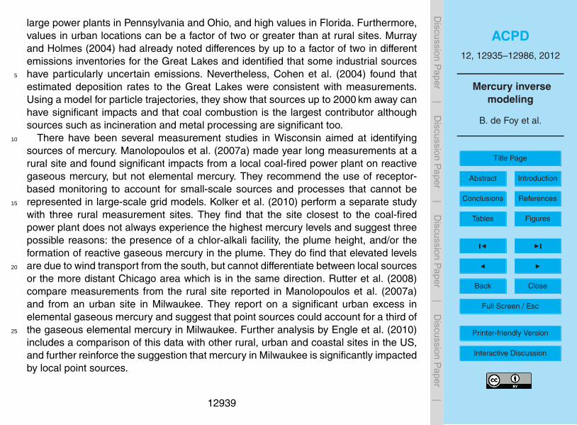
Where Ra is the error covariance matrix corresponding to the sensitivity matrix H, andRb is the error covariance matrix on the emissions factors in x.

The sensitivity matrix H can be composed of multiple components, as was done inRigby et al. (2011). In this work, we combine the sensitivities from the back-trajectoriesobtained using WRF-FLEXPART, the sensitivities from forward simulations using CAMx5

and the sensitivities due to background values:

H = (HRTA, HCAMx, HBkg) (5)

x = (xRTA, xCAMx, xBkg)T (6)

xRTA contains the gridded emissions parameters, and HRTA is the Residence Time10

Analysis from WRF-FLEXPART that contains the impacts of the emissions in a gridcell on the concentrations at the measurement site. xCAMx are the scaling factors onthe concentrations obtained from CAMx simulations contained in HCAMx. Finally, thebackground values are contained in xBkg and HBkg. This can be limited to a singlevalue or be expanded for a varying background in time.15

If we have a priori values xo for the emissions factors x, we modify the equationsto solve for adjustments to the a priori emissions factors (x′) instead of solving foremissions factors directly:

x′ = x−xo (7)

y′ = y −Hxo (8)20

In order to simplify the solution of the system, the cost function of the emissionsvector (Jemiss) can be folded into the Jobs term by augmenting the sensitivity matrix Hwith diagonal terms and the observation vector y with zero values, so that we have:

J = (H′′x−y′′)TR−1(H′′x−y′′) (9)25

Where H′′ = (H, D) and y′′ = (y, xzero) are the augmented versions of H and y (or of

H′ and y′ if using a priori emissions). D is a diagonal matrix the size of x, and xzero is

a vector of zero values. The new error covariance matrix is given by R = (Ra, Rb).12946





ACPD12, 12935–12986, 2012


B. de Foy et al.

Title Page



Tables Figures

J I

J I

Back Close

Full Screen / Esc



Discussion

Paper

|D

iscussionP

aper|

Discussion

Paper

|D

iscussionP

aper|

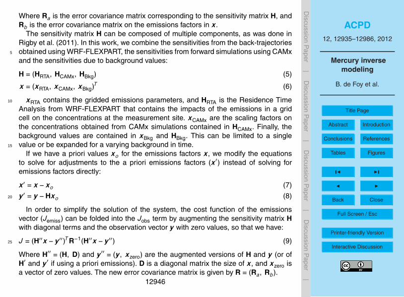
The error covariance matrices are often taken to be diagonal matrices because ofa lack of information on the off-diagonal elements (Brioude et al., 2011; Stohl et al.,2009). In this case, Eq. (9) simplifies to a linear least-squares problem, where eachrow i is scaled by a scaling factor si determined from the diagonal terms of the errorcovariance matrix R.5

J = ‖s · (H′′x−y′′)‖2 (10)

The purpose of using this formulation is to simplify the equation to a single least-squares problem so that constraints can be applied easily to the emissions vector x.Solution methods for Eq. (4) will generate negative emission values by default (Stohlet al., 2009; Brioude et al., 2011). These corrupt the solution by obtaining an excellent10

fit for the linear model (Eq. 2) from a combination of unphysical values. Stohl et al.(2009) solve this problem by iteration. After each solution, the error covariance termsare adjusted to force the posterior emissions closer to the a priori emissions for thosepoints that would be negative. Brioude et al. (2011) address the problem by workingwith the log of the concentrations. In this work, we apply constraints to the solution of15

the linear least-squares problem directly to Eq. (10). In this way, the solution x can befound by straightforward application of the Matlab function lsqlin.

The vector s contains scaling terms for individual contributions from the vector x.Initially, values are assumed to be homogeneous within Jobs and Jemiss, which meansthat in practice si for the observations are set to 1 and those for the emissions factors20

are set to a regularization parameter α (Brioude et al., 2011; Henze et al., 2009). Thisparameter excercises a constraint on the magnitude of the emissions factors (or onthe adjustments when using a priori emissions). Because it relates the importance ofthe cost function of the measurements with that of the emissions factors it is not adimensionless number. Based on testing, it was set to a value of 1×10−4. After the first25

solution of the least-squares problem, the magnitude of the residual in Eq. (2) is usedto refine estimates of si . Observation times that have a residual larger than 3 times

12947





ACPD12, 12935–12986, 2012


B. de Foy et al.

Title Page



Tables Figures

J I

J I

Back Close

Full Screen / Esc



Discussion

Paper

|D

iscussionP

aper|

Discussion

Paper

|D

iscussionP

aper|

the standard deviation of the residual values are assigned a scaling factor of 0. Thisprocess converges on stable values of s after 2 to 4 iterations.

When obtaining the solution, one must pay close attention to the units of the system.The measurements y are in units of ngm−3 and the emissions x were calculated inunits of lbyr−1 to be consistent with the EPA emissions inventories. The Residence5

Time Analysis matrix H is in units of particle ·hours. This means that we need to scalethe product Hx by a factor with units of ng lb−1 · yrh−1 · 1(particle · volume)−1. For thelast term on the right we use the maximum number of particles in a simulation (1000 inour case) multiplied by the volume of the grid cells in the Residence Time Analysis. Theheight of the cells used for counting particles to obtain the RTA matrix must be chosen10

to be large enough to have a sufficient number of particle counts, and small enough toprovide a value that is related to the measurements which are surface concentrations.In practice, we choose a value of 1000 m which corresponds to the mixing height forthe time scales corresponding to the transport distances in the polar grid used.

To obtain a posteriori confidence intervals on the results, we use the bootstrap15

method. Multiple instances of the model are run with a random selection, with re-placement, of both the times and the emission factors. Measurement times used in theanalysis are randomly selected leading to a modified measurement vector y and cor-responding selection of the rows in H. Emission factors from the particle grid (xRTA) arealso randomly selected leading to rearrangement of the columns of HRTA. The CAMx20

time series are used with a probability of 75 % in any given simulation. In practice thisis done by resetting columns of HCAMx to zero with a probability of 25 %.

3 Results

Before describing the inverse method, we present a preliminary analysis using simplermethods. Figure 4 shows the time series of elemental gaseous mercury concentrations,25

which was analyzed by Rutter et al. (2008). As described above, there are 3594 datapoints which are hourly concentrations measured on alternate hours from 28 June

12948





ACPD12, 12935–12986, 2012


B. de Foy et al.

Title Page



Tables Figures

J I

J I

Back Close

Full Screen / Esc



Discussion

Paper

|D

iscussionP

aper|

Discussion

Paper

|D

iscussionP

aper|

2004 to 11 May 2005 (inclusive). There are a combination of features ranging from thehourly scale to the daily and weekly scale. High peaks of short duration suggest narrowplumes from point sources. These were estimated to make up one third of the GEMin Rutter et al. (2008). Longer peaks such as in the second half of November 2004 orduring April 2005 suggest larger scale phenomena.5

Figure 5 shows windroses corresponding to low, high and very high GEM levels.The dominant winds during concentrations in the bottom 50 % are from the northwest.For high concentrations, defined as being in the 50 % to 95 % range, the winds arepredominantly from the south-southwest and from the north-northeast. The top 5 %of concentrations take place when there are winds from the northeast and from the10

southwest. The bars in the windroses are colored by time of day and show that thenortheast winds are associated with afternoon winds whereas the southwest winds aremore likely to be before sunrise.

Figure 6 shows the Residence Time Analysis and the Concentration Field Analysisfor a domain covering most of WRF domain 1 for the entire time period. The RTA15

is in agreement with the windroses and shows that the dominant wind transport toMilwaukee is from the northwest, from the northeast over Lake Michigan and fromthe south-southwest through Illinois. The southeast area has the smallest contributionto airmass transport at the receptor site. The CFA shows that there are unlikely tobe significant mercury sources to the northwest, in agreement with the windroses.20

The northeast signature in the windroses corresponds to a significant potential sourceregion over the Great Lakes in the CFA analysis. Finally, south-southwest transport ofmercury to Milwaukee corresponds to transport from industrial regions to the south.As CFA does not distinguish easily between positions along the plume path, thesecould be a combination of local sources south of the measurement site, more distant25

sources from the Chicago area or sources beyound that. Althouh the airmass does notfrequently come over the Ohio River Valley, when it does it is associated with high GEMlevels.

12949





ACPD12, 12935–12986, 2012


B. de Foy et al.

Title Page



Tables Figures

J I

J I

Back Close

Full Screen / Esc



Discussion

Paper

|D

iscussionP

aper|

Discussion

Paper

|D

iscussionP

aper|

3.1 Synthetic inverse

The inverse method was tested using synthetic data corresponding to continuous emis-sions from a point 213 km to the northwest of the measurement site. Synthetic concen-trations were simulated using CAMx as input for the inversion. Residual scaling wasapplied and converged on the fourth iteration, with 177 measurements excluded from5

the analysis (out of a total of 7657). Figure 7 shows the map of the inverse emis-sions, clearly showing that the model correctly identifies the source cell. The emissionstrength from the actual emission grid cell was underestimated by 25 %. If we includethe neighboring grid cells in the emission strength, then the underestimate is reducedto 18 %. Because the model simulates emissions from cells further away, there is an10

overall over-estimation of the emissions by 21 %. Taking emissions from the 9 grid cellsaround the source, we find that 68 % of the emissions in the inversion come from thecorrect area.

One can see from the emissions map (Fig. 7) that the model is better at resolvingthe direction of the source than the distance from the source. Furthermore, the model15

has a tendency to overestimate distant sources. This happens if the particular grid cellshappens to have a single impact that coincides with a high concentration peak at themeasurement site. There are three ways of mitigating this problem in the current setup.The first is by using a polar grid with increasing cell sizes. This makes it less likely tohave a chance correlation between the RTA and the concentrations. The second is to20

use iterative residual scaling which prevents the scheme from trying to match peaksthat it cannot resolve. The third is to use the regularization parameter α which balancesthe cost function between the measurements and the emissions factors. By increasingthis, the model will reduce the overal amount of predicted emissions.

3.2 Full inverse25

The inversion algorithm was run on the actual data (3594 data points) using the polargrid consisting of 360 grid cells, the 9 CAMx concentration time series for the forest fires

12950





ACPD12, 12935–12986, 2012


B. de Foy et al.

Title Page



Tables Figures

J I

J I

Back Close

Full Screen / Esc



Discussion

Paper

|D

iscussionP

aper|

Discussion

Paper

|D

iscussionP

aper|

domains, one CAMx concentration time series for the lake surface emissions and a sin-gle value for the background. The augmented matrix H′′ contains a further 360 rowswith the weighting factors in the diagonal. This leads to the solution of a linear systemof equations with dimensions of 3954×371. Because the actual inversion takes of theorder of one second to run on a desktop, it can be easily carried out for 100 boot-5

strapped simulations of 5 iterations each. The 5 iterations allow the residual scalingto converge and the 100 bootstrapped simulations provide a measure of uncertaintyon the solution vector x. For the simulations presented we do not use a priori emis-sions, instead leaving the inversion algorithm to identify source regions irrespective ofprevious estimates.10

Figure 8 shows the inverse emissions grids in units of kgyr−1, using the median ofthe 100 bootstrapped runs. Table 3 shows the total emissions, tabulated according tothe geographic region for the domains shown in Fig. 11. The table also shows the lowerquartile and upper quartile values of the bootstrapped simulations which represent ameasure of the variability of the results.15

The largest sources are from grid cells over the Ohio River Valley to the southeast,which is an area known for its large coal-fired power plants. Overall, the model esti-mates emissions of 23 000 kgyr−1 from the southeast domain. The southwest domainemissions are estimated to be 24 000 kgyr−1 from a larger number of grid cells corre-sponding to emissions from a broader area. After this, the northeast domain accounts20

for 13 000 kgyr−1 coming from upper Michigan, Eastern Canada, the US Northeast,Lake Huron and Lake Superior. The remaining domains have lower estimated emis-sions. To the northwest there are 6000 kgyr−1 from the upper Great Plains. Closer in,there are 3500 kgyr−1 from regional sources to the west and 6000 kgyr−1 from regionalsources to the south, which include Chicago. The local domain counts sources within25

a 50 km radius of the measurement site, for a total of 1000 kgyr−1.Figure 9 shows histograms of the scaling factors applied to the CAMx simulated

timeseries of forest fires and lake surface emissions. Median, lower quartile and upperquartile values are shown in Table 4. The lake surface emissions have a very reliable

12951





ACPD12, 12935–12986, 2012


B. de Foy et al.

Title Page



Tables Figures

J I

J I

Back Close

Full Screen / Esc



Discussion

Paper

|D

iscussionP

aper|

Discussion

Paper

|D

iscussionP

aper|

scaling factor with a median value of 1.9 and an interquartile range of 1.7 to 2.2. Thissuggests that the results are robust relative to the selection of time periods and arenot sensitive to the selection of grid points or forest fires timeseries included in theinversion.

The forest fires factors vary across the domains shown in Fig. 3. The most reliable5

result is a median factor of 3.9 (inter-quartile range 3.1 to 4.5) for fires in the eastdomain excluding WRF domain 2. Fires for the north central domain have consistentscaling factors of 2.6 on average (IQR 2.2 to 3.3). After these, the south central andsoutheast domain have scaling factors of 1.2 (IQR 0.8 to 1.6) and 1.1 (IQR 0.6 to 1.6),respectively. The scaling factor for the West domain has a large variation, ranging from10

3.9 to 10.1, but with the full range extending to zero values. The rest of the domainshave very low scaling factors. Northern Canada has an inter-quartile range of 0.02 to0.17 and Alaska and the pacific northwest have zero values. Fires within WRF domain2, close to the measurement site, also have scaling factors of 0.

Figure 10 shows the inverted time series (given by Hx) along with the original mea-15

surements (y). The median Pearson correlation coefficient (r) between the two is 0.39for the complete time series and 0.58 when excluding the times removed by the resid-ual scaling.

The background value determined from the model is 1.99 ngm−3 (IQR 1.98 to2.01 ngm−3) and is very stable across model configurations. Rutter et al. (2008) mea-20

sured background concentrations of 1.5 ngm−3 at a rural site 150 km to the west andannual average concentrations of 1.6 ngm−3. This suggests that the discrepancy of0.49 ngm−3 can be separated into 0.1 ngm−3 from regional background and 0.4 ngm−3

due to local sources in and around Milwaukee.The time series of the contribution from the gridded emissions, the forest fires and the25

lake surface emissions are shown in the bottom panel of Fig. 10. The gridded emissionsare assumed to be constant throughout the year and vary at both daily and synoptictime scales depending on the prevailing wind directions. The forest fires has a clearseasonal component, as expected. The highest contribution occurs during the high

12952





ACPD12, 12935–12986, 2012


B. de Foy et al.

Title Page



Tables Figures

J I

J I

Back Close

Full Screen / Esc



Discussion

Paper

|D

iscussionP

aper|

Discussion

Paper

|D

iscussionP

aper|

GEM event of April 2005 as well as during the smaller but more frequent events duringfall 2004. The lake surface emissions are temperature dependent and therefore havea similar seasonal pattern, except that they are less influenced by individual events.Compared with the forest fires impacts, the lake surface also contributes to the April2005 event, but it has a more continuous impact during the late summer of 2004. There5

are sporadic lake surface impacts at the measurement site throughout the fall, winterand spring.

3.3 Impacts of estimated source groups on average GEM concentrations

Table 5 shows the impacts of specific source groups on the average GEM concentra-tions at the receptor site. The results for the grid domains are aggregated from the grid10

cell impacts shown in Fig. 11. The table shows the median values and the inter-quartilerange from the bootstrapped runs. Figure 12 shows the impacts from the inverse modelfor the Great Lakes, the forest fires and the gridded emissions by geographical do-main. Overall, the measurements have an average concentration of 2.48 ngm−3 andthe model inversion timeseries has an average of 2.33 ngm−3, leaving an unaccounted15

for gap of 150 pgm−3. The greatest contributions to the inverted time series are from theglobal background (1.5 ngm−3) and from the additional local and regional background(0.49 ngm−3).

This leaves contributions of 188 pgm−3 from the gridded emissions, 86 pgm−3 fromthe forest fires and 61 pgm−3 from the lake surface emissions. The impacts due to the20

gridded emissions, shown in Fig. 11 are the product of the estimated emissions of agrid cell times the impact of that grid cell on the measurement site, obtained from theResidence Time Analysis. The large sources from the southeast and the southwestcan be seen to contribute 16 pgm−3 and 23 pgm−3, which are low values because theair mass in Milwaukee does not often come from those directions (see Fig. 6). The25

middle panel of Fig. 11 shows that the regional impacts from the south are mainly dueto the Chicago area with an estimated contribution of 30 pgm−3. The main contributorfrom the gridded emissions are the local sources with impacts of 64 pgm−3. These

12953





ACPD12, 12935–12986, 2012


B. de Foy et al.

Title Page



Tables Figures

J I

J I

Back Close

Full Screen / Esc



Discussion

Paper

|D

iscussionP

aper|

Discussion

Paper

|D

iscussionP

aper|

can be seen in the right panel of Fig. 11 to be close to the source as well as to thesouthwest of the measurement site, which is the direction of the Menomonee valleyindustrial corridor.

The fire contributions are mainly from the east domain, with average concentrationsof 46 pgm−3. Next come the southeast, south central and north central domains with5

contributions of approximately 10 pgm−3. As noted above, the contributions from thewest have a large uncertainty range, as do the ones from Northern Canada. The con-tributions from the the local fires, the pacific northwest and Alaska were all 0.

4 Discussion

4.1 Comparison with the toxic release inventory and national emissions10

inventory

The estimated gridded emissions in Fig. 8 can be compared with the US emissionsfrom the 2004 Toxic Release Inventory (TRI) and those from the 2002 National Emis-sions Inventory (NEI), as shown in Fig. 13. TRI version 10 files were obtained fromthe US Environmental Protection Agency’s website. These contain separate emission15

values for mercury and mercury compounds, which have been added together in thepresent work. The 2002 NEI Hazardous Air Pollutant inventory was obtained for pointsources, using the files dated 23 January 2008 also available from the EPA’s web-site. These contain separate values for elemental mercury, gaseous divalent mercury,particulate divalent mercury as well as two additional categories called “mercury” and20

“mercury and compounds”. Here we use the emissions of elemental mercury as wellas the total of all mercury types put together.

Total emissions are listed by domain in Table 3 for comparison with the model results.In terms of spatial distribution, the Ohio River Valley clearly stands out as it did in themodel results. The two different inventories are in agreement on these sources with25

magnitudes within a factor of 2 of each other. The model estimated sources were in the

12954





ACPD12, 12935–12986, 2012


B. de Foy et al.

Title Page



Tables Figures

J I

J I

Back Close

Full Screen / Esc



Discussion

Paper

|D

iscussionP

aper|

Discussion

Paper

|D

iscussionP

aper|

range (IQR) of 19 761 to 26 391 kgyr−1, compared with TRI emissions of 17 658 kgyr−1

and NEI emissions of 6035 kgyr−1 for elemental mercury and 25 603 kgyr−1 countingall mercury emission types.

There are emissions from the southwest, but these are smaller than would expectedfrom the model by at least a factor of 2. A similar situation holds for the northwest5

and for the regional sources, with model results about 3 times higher than the TRI.The values for the northeast cannot be compared directly, as they do not include theemissions from Canada. Finally, the local emissions estimated by the model are a factorof 4 higher than the TRI, and a factor of 5 higher than the total mercury emissions fromthe NEI.10

Part of the discrepancy maybe due to the fact that the inventories only include pointsources for mercury. Had it been possible, including area sources could reduce the dif-ference with the inverse model results. On the other hand, the synthetic test revealedthat in the case of a simple source, the model tended to overestimate total emissionseven though it identified the location of the source accurately. It is therefore reasonable15

to place greater confidence in the spatial pattern and relative magnitude of the emis-sions than in the absolute emission totals. Nevertheless, on balance the analysis doessuggest that the emissions inventories underestimate elemental mercury emissionsfrom sources other than the large coal-fired power plants.

4.2 Time scale analysis20

Table 5 above showed that 6 % of GEM was unaccounted for by the model. In orderto identify what this might be due to, we perform a time scale analysis as describedby Hogrefe et al. (2003) and Hogrefe et al. (2001). We use the Kolmogorov-Zurbenkofilter to separate the time series according to the temporal scale of the signal. Theconcentrations are split into intra-day, diurnal, synoptic and seasonal components. Note25

that for simplicity, we use the same coefficients as Hogrefe et al. (2003), althoughthat means that our categories include longer timescales because we have data on

12955





ACPD12, 12935–12986, 2012


B. de Foy et al.

Title Page



Tables Figures

J I

J I

Back Close

Full Screen / Esc



Discussion

Paper

|D

iscussionP

aper|

Discussion

Paper

|D

iscussionP

aper|

alternate hours rather than every hour. The contribution of each temporal componentto the full time series is obtained by calculating the variance of each component as afraction of the sum of the variances of all the components.

Table 6 shows the results for the measurement time series, the inverted time seriesand the residual. This shows clearly that the measurements have components that5

vary across the whole range of times scales with roughly similar contributions fromeach category. In contrast, the inverted time series is much lower on the intra-daycomponent, which accounts for 7 % instead of 29 % of the variance. Correspondingly,the synoptic scale accounts for a greater fraction of the variance (43 % instead of 24 %).For the residual, the components are highest in the intra-day scale and lowest in the10

seasonal scale.This demonstrates that the inverse model is missing some of the high frequency

components of the timeseries. These are due to short spikes in concentrations, whichare most likely to be local sources where the plume has not had as much time to dilute.This suggests that the method is more likely to underestimate sources that are close by.15

Consequently, it can be inferred that a significant fraction of the unaccounted mercuryis due to local sources.

4.3 Emission types

The results of this analysis suggest that the emissions of GEM from the lake surfacesare two times higher than those calculated in Sect. 2.4. As noted above, there is con-20

siderable spread in the measured concentrations of dissolved gaseous mercury. Theinverse model suggests that average values may be towards the higher end of thereported range, well above the 30 pgl−1 used in the calculations. This would suggestaverage fluxes in the range of 4 to 5 ngm−2 h−1 and total emissions from the GreatLakes of 12 000 to 14 000 kg of GEM for the time period of the study.25

Forest fires were found to have a clearly detectable signal in the GEM time series,with total impacts around 30 % higher than the lake surface impacts. Most of these aredue to emissions in the east domain which includes a large part of the midwest, the

12956





ACPD12, 12935–12986, 2012


B. de Foy et al.

Title Page



Tables Figures

J I

J I

Back Close

Full Screen / Esc



Discussion

Paper

|D

iscussionP

aper|

Discussion

Paper

|D

iscussionP

aper|

northeast and Southeastern Canada. The inverse model suggests that emissions fromthis area could be underestimated by a factor of 3 to 4. The model further suggests thatemissions in the north central domain could be underestimated by a factor of 2 to 3, butthat estimates of the emissions form the south central and southeast domains are ofthe correct magnitude. The domains further away were found to have nil or variable im-5

pacts. This could be because there is not enough data in the inversion, either becausethose areas do not influence the measurement site often enough, or because the levelof the impacts is too low relative to other sources. Finally, the FINN model estimatedreleases of 1383kg of mercury in WRF domain 2, close to the measurement site. Theinverse model did not identify any impacts from these. This could be because local10

sources have short, sharp peaks which can easily suffer from mismatches betweenthe model and the measurements or because the diurnal distribution of the emissionsis more important for local sources. As with the gridded emissions, the inverse modeldoes a better job of identifying sources that are further away than near-field ones.

There was one large episode of elevated GEM concentrations starting on 12 Novem-15

ber 2004 and lasting until the end of the month which is not accounted for in the inver-sion, see Fig. 10. Levels rose rapidly to between 4 and 6 ngm−3 and decayed slowlyover the next 2 weeks. This suggests a large regional source, but the event is puz-zling because it lasted over a variety of wind patterns with shifting air masses fromboth the north and the south. Volcanoes can emit large amounts of mercury during20

explosions (Bagnato et al., 2011) and could be a possible source. Mount St. Helensin Washington State had renewed eruptions between September 2004 and December2005 and could possibly be a factor in this event (Sherrod et al., 2008). We simulatedforward emissions from the volcano using CAMx in combination with the large WRFdomain used for forest fires. Although this source cannot be ruled out, the results did25

not provide strong evidence in support of this hypothesis.Grımsvotn in Iceland had a week long eruption starting on 1 November 2004 (Thor-

darson and Larsen, 2007). We performed forward particle simulations using FLEX-PART based on wind fields from the Global Forecast System. Although the arrival

12957





ACPD12, 12935–12986, 2012


B. de Foy et al.

Title Page



Tables Figures

J I

J I

Back Close

Full Screen / Esc



Discussion

Paper

|D

iscussionP

aper|

Discussion

Paper

|D

iscussionP

aper|

time matched the episode in the time series, the simulated concentrations lasted muchlonger than the measured episode itself. It would therefore seem that such a distantsource cannot be responsible for such a clearly defined event. Nevertheless, furtheranalysis of this event may be warranted especially if it can be expanded with concur-rent measurements from different sites.5

5 Conclusions

This paper developed a hybrid inversion scheme based on particle back-trajectoriesand forward grid modeling to evaluate sources of elemental mercury using atmosphericmeasurements in Milwaukee. The method provided estimates of source strengths aswell as source impacts at the measurement site. Using bootstrapping, the method fur-10

ther provided confidence intervals on the results.Identifying local point sources is a particular challenge. The analysis therefore re-

quired a combination of analysis methods including meteorological analysis, concen-tration field analysis and time scale analysis to supplement the inverse method.

In agreement with past studies, it was found that mercury levels are impacted by15

sources at multiple scales, from small local sources to large distant point sources. Theinverted strengths of the coal-fired power plants was in good agreement with currentinventories, but other sources seem to be under-represented. These may include wastedisposal and incineration as well as metal processing.

The impacts of emissions from the lake surface and from forest fires could be clearly20

seen in the model inversion. These suggest that emissions from both of these sourcesare larger than predicted by current emissions models and that they are a significantsource of elemental gaseous mercury.

As the inversion uses a hybrid model, it is straightforward to simulate candidatesources using a grid model and include them in the analysis. Soil and vegetation25

sources could be included in the same way as the lake surface sources. Further exam-ples would depend on the location of the measurement site and could include testing

12958





ACPD12, 12935–12986, 2012


B. de Foy et al.

Title Page



Tables Figures

J I

J I

Back Close

Full Screen / Esc



Discussion

Paper

|D

iscussionP

aper|

Discussion

Paper

|D

iscussionP

aper|

the possibility of emissions from melting snow or the magnitude of emissions from goldmining and underground coal fires.

Acknowledgements. This manuscript was made possible by EPA grant number RD-83455701.Its contents are solely the responsibility of the grantee and do not necessarily represent theofficial views of the EPA. Further, the EPA does not endorse the purchase of any commercial5

products or services mentioned in the publication. The initial mercury measurements werefunded by US EPA STAR Grant # R829798. We are also grateful to the US EPA for making theNational Emissions Inventory and Toxic Release Inventory available, and to the US NationalClimatic Data Center for the meteorological data.

References10

Akagi, S. K., Yokelson, R. J., Wiedinmyer, C., Alvarado, M. J., Reid, J. S., Karl, T., Crounse, J. D.,and Wennberg, P. O.: Emission factors for open and domestic biomass burning for use inatmospheric models, Atmos. Chem. Phys., 11, 4039–4072, doi:10.5194/acp-11-4039-2011,2011. 12945

Ashbaugh, L. L., Malm, W. C., and Sadeh, W. Z.: A residence time probability analysis of sul-15

fur concentrations at Grand-Canyon-National-Park, Atmos. Environ., 19, 1263–1270, 1985.12942

Bagnato, E., Aiuppa, A., Parello, F., Allard, P., Shinohara, H., Liuzzo, M., and Giudice, G.: Newclues on the contribution of Earth’s volcanism to the global mercury cycle, B. Volcanol., 73,497–510, doi:10.1007/s00445-010-0419-y, 2011. 1295720

Bash, J. O.: Description and initial simulation of a dynamic bidirectional air-surface exchangemodel for mercury in Community Multiscale Air Quality (CMAQ) model, J. Geophys. Res.-Atmos., 115, D06305, doi:10.1029/2009JD012834, 2010. 12938

Bash, J. O. and Miller, D. R.: A relaxed eddy accumulation system for measur-ing surface fluxes of total gaseous mercury, J. Atmos. Ocean. Tech., 25, 244–257,25

doi:10.1175/2007JTECHA908.1, 2008. 12938Bash, J., Miller, D., Meyer, T., and Bresnahan, P.: Northeast United States and Southeast

Canada natural mercury emissions estimated with a surface emission model, Atmos. En-viron., 38, 5683–5692, doi:10.1016/j.atmosenv.2004.05.058, 2004. 12937

12959





http://dx.doi.org/10.5194/acp-11-4039-2011

http://dx.doi.org/10.1007/s00445-010-0419-y

http://dx.doi.org/10.1029/2009JD012834

http://dx.doi.org/10.1175/2007JTECHA908.1

http://dx.doi.org/10.1016/j.atmosenv.2004.05.058

ACPD12, 12935–12986, 2012


B. de Foy et al.

Title Page



Tables Figures

J I

J I

Back Close

Full Screen / Esc



Discussion

Paper

|D

iscussionP

aper|

Discussion

Paper

|D

iscussionP

aper|

Brioude, J., Kim, S.-W., Angevine, W. M., Frost, G. J., Lee, S.-H., McKeen, S. A., Trainer, M.,Fehsenfeld, F. C., Holloway, J. S., Ryerson, T. B., Williams, E. J., Petron, G., and Fast, J. D.:Top-down estimate of anthropogenic emission inventories and their interannual variabilityin Houston using a mesoscale inverse modeling technique, J. Geophys. Res.-Atmos., 116,D20305, doi:10.1029/2011JD016215, 2011. 12945, 129475

Bullock, Jr., O. R., Atkinson, D., Braverman, T., Civerolo, K., Dastoor, A., Davignon, D., Ku, J.-Y., Lohman, K., Myers, T. C., Park, R. J., Seigneur, C., Selin, N. E., Sistla, G., and Vi-jayaraghavan, K.: The North American Mercury Model Intercomparison Study (NAMMIS):study description and model-to-model comparisons, J. Geophys. Res.-Atmos., 113, D17310,doi:10.1029/2008JD009803, 2008. 1293810

Carroll, M., Townshend, J., Hansen, M., DiMiceli, C., Sohlberg, R., and Wurster, K.: Vegetativecover conversion and vegetation continuous fields, in: Land Remote Sensing and Global En-vironmental Change: NASA’s Earth Observing System and the Science of Aster and MODIS,edited by: Ramachandran, B., Justice, C. O., and Abrams, M., Springer-Verlag, Chapter 32,725–745, Springer-Verlag, New York, USA, doi:10.1007/978-1-4419-6749-7, 2011. 1294515

Cheng, I., Lu, J., and Song, X.: Studies of potential sources that contributedto atmospheric mercury in Toronto, Canada, Atmos. Environ., 43, 6145–6158,doi:10.1016/j.atmosenv.2009.09.008, 2009. 12940

Cheng, I., Zhang, L., Blanchard, P., Graydon, J. A., and St. Louis, V. L.: Source-receptor rela-tionships for speciated atmospheric mercury at the remote Experimental Lakes Area, north-20

western Ontario, Canada, Atmos. Chem. Phys., 12, 1903–1922, doi:10.5194/acp-12-1903-2012, 2012. 12940

Ci, Z., Zhang, X., and Wang, Z.: Elemental mercury in coastal seawater of YellowSea, China: temporal variation and air-sea exchange, Atmos. Environ., 45, 183–190,doi:10.1016/j.atmosenv.2010.09.025, 2011a. 1294325

Ci, Z. J., Zhang, X. S., Wang, Z. W., Niu, Z. C., Diao, X. Y., and Wang, S. W.: Distribution andair-sea exchange of mercury (Hg) in the Yellow Sea, Atmos. Chem. Phys., 11, 2881–2892,doi:10.5194/acp-11-2881-2011, 2011b. 12943

Cohen, M., Artz, R., Draxler, R., Miller, P., Poissant, L., Niemi, D., Ratte, D., Deslauriers, M.,Duval, R., Laurin, R., Slotnick, J., Nettesheim, T., and McDonald, J.: Modeling the atmo-30

spheric transport and deposition of mercury to the Great Lakes, Environ. Res., 95, 247–265,doi:10.1016/j.envres.2003.11.007, 2004. 12939

12960





http://dx.doi.org/10.1029/2011JD016215

http://dx.doi.org/10.1029/2008JD009803

http://dx.doi.org/10.1007/978-1-4419-6749-7







http://dx.doi.org/10.1016/j.envres.2003.11.007

ACPD12, 12935–12986, 2012


B. de Foy et al.

Title Page



Tables Figures

J I

J I

Back Close

Full Screen / Esc



Discussion

Paper

|D

iscussionP

aper|

Discussion

Paper

|D

iscussionP

aper|

Doran, J. C., Fast, J. D., Barnard, J. C., Laskin, A., Desyaterik, Y., and Gilles, M. K.: Applicationsof lagrangian dispersion modeling to the analysis of changes in the specific absorption ofelemental carbon, Atmos. Chem. Phys., 8, 1377–1389, doi:10.5194/acp-8-1377-2008, 2008.12942

Engle, M. A., Tate, M. T., Krabbenhoft, D. P., Schauer, J. J., Kolker, A., Shanley, J. B., and5

Bothner, M. H.: Comparison of atmospheric mercury speciation and deposition at ninesites across Central and Eastern North America, J. Geophys. Res.-Atmos., 115, D18306,doi:10.1029/2010JD014064, 2010. 12938, 12939

Enting, I. G.: Inverse Problems in Atmospheric Constituent Transport, Cambridge UniversityPress, Cambridge University Press, Cambridge, UK, 2002. 1294510

ENVIRON: CAMx, comprehensive air quality model with extensions, User’s Guide, Tech. Rep.Version 5.40, ENVIRON International Corporation, ENVIRON International Corporation, No-vato, California, USA, 2011. 12944

Fast, J. D. and Easter, R.: A Lagrangian particle dispersion model compatible with WRF, in: 7thWRF User’s Workshop, Boulder, CO, 19–22 June 2006, Abstract P6.2, 2006. 1294215

de Foy, B., Lei, W., Zavala, M., Volkamer, R., Samuelsson, J., Mellqvist, J., Galle, B.,Martınez, A.-P., Grutter, M., Retama, A., and Molina, L. T.: Modelling constraints on the emis-sion inventory and on vertical dispersion for CO and SO2 in the Mexico City MetropolitanArea using Solar FTIR and zenith sky UV spectroscopy, Atmos. Chem. Phys., 7, 781–801,doi:10.5194/acp-7-781-2007, 2007. 1294220

de Foy, B., Zavala, M., Bei, N., and Molina, L. T.: Evaluation of WRF mesoscale simulationsand particle trajectory analysis for the MILAGRO field campaign, Atmos. Chem. Phys., 9,4419–4438, doi:10.5194/acp-9-4419-2009, 2009. 12942

de Foy, B., Smyth, A. M., Thompson, S. L., Gross, D. S., Olson, M. R., Sager, N., andSchauer, J. J.: Sources of nickel, vanadium and black carbon in aerosols in Milwaukee, At-25

mos. Environ., submitted, 2012. 12941Friedl, M. A., Sulla-Menashe, D., Tan, B., Schneider, A., Ramankutty, N., Sibley, A., and

Huang, X.: MODIS collection 5 global land cover: algorithm refinements and characteriza-tion of new datasets, Remote Sens. Environ., 114, 168–182, doi:10.1016/j.rse.2009.08.016,2010. 1294430

Gbor, P., Wen, D., Meng, F., Yang, F., Zhang, B., and Sloan, J.: Improved modelfor mercury emission, transport and deposition, Atmos. Environ., 40, 973–983,doi:10.1016/j.atmosenv.2005.10.040, 2006. 12938

12961






http://dx.doi.org/10.1029/2010JD014064



http://dx.doi.org/10.1016/j.rse.2009.08.016


ACPD12, 12935–12986, 2012


B. de Foy et al.

Title Page



Tables Figures

J I

J I

Back Close

Full Screen / Esc



Discussion

Paper

|D

iscussionP

aper|

Discussion

Paper

|D

iscussionP

aper|

Gbor, P. K., Wen, D., Meng, F., Yang, F., and Sloan, J. J.: Modeling of mercury emis-sion, transport and deposition in North America, Atmos. Environ., 41, 1135–1149,doi:10.1016/j.atmosenv.2006.10.005, 2007. 12938

Giglio, L., Descloitres, J., Justice, C., and Kaufman, Y.: An enhanced contextual fire de-tection algorithm for MODIS, Remote Sens. Environ., 87, 273–282, doi:10.1016/S0034-5

4257(03)00184-6, 2003. 12944Han, Y., Holsen, T., Hopke, P., and Yi, S.: Comparison between back-trajectory based model-

ing and Lagrangian backward dispersion modeling for locating sources of reactive gaseousmercury, Environ. Sci. Technol., 39, 1715–1723, doi:10.1021/es0498540, 2005. 12940

Han, Y.-J., Holsen, T. M., and Hopke, P. K.: Estimation of source locations of total gaseous10

mercury measured in New York State using trajectory-based models, Atmos. Environ., 41,6033–6047, doi:10.1016/j.atmosenv.2007.03.027, 2007. 12940

Hansen, M., Townshend, J., Defries, R., and Carroll, M.: Estimation of tree cover using MODISdata at global, continental and regional/local scales, Int. J. Remote Sens., 26, 4359–4380,2005. 1294515

Hansen, M. C., DeFries, R. S., Townshend, J. R. G., Carroll, M., Dimiceli, C., andSohlberg, R. A.: Global percent tree cover at a spatial resolution of 500 meters: firstresults of the MODIS vegetation continuous fields algorithm, Earth Interact., 7, 1–15,doi:10.1175/1087-3562(2003)007<0001:GPTCAA>2.0.CO;2 2003. 12945

Henze, D. K., Seinfeld, J. H., and Shindell, D. T.: Inverse modeling and mapping US air quality20

influences of inorganic PM2.5 precursor emissions using the adjoint of GEOS-Chem, Atmos.Chem. Phys., 9, 5877–5903, doi:10.5194/acp-9-5877-2009, 2009. 12947

Hoelzemann, J., Schultz, M., Brasseur, G., Granier, C., and Simon, M.: Global wildland fireemission model (GWEM): evaluating the use of global area burnt satellite data, J. Geophys.Res.-Atmos., 109, D14S04, doi:10.1029/2003JD003666, 2004. 1294525

Hogrefe, C., Rao, S., Kasibhatla, P., Hao, W., Sistla, G., Mathur, R., and McHenry, J.: Evalu-ating the performance of regional-scale photochemical modeling systems: Part II – ozonepredictions, Atmos. Environ., 35, 4175–4188, doi:10.1016/S1352-2310(01)00183-2, 2001.12955

Hogrefe, C., Vempaty, S., Rao, S., and Porter, P.: A comparison of four techniques for30

separating different time scales in atmospheric variables, Atmos. Environ., 37, 313–325,doi:10.1016/S1352-2310(02)00897-X, 2003. 12955

12962






http://dx.doi.org/10.1016/S0034-4257(03)00184-6

http://dx.doi.org/10.1016/S0034-4257(03)00184-6

http://dx.doi.org/10.1016/S0034-4257(03)00184-6

http://dx.doi.org/10.1021/es0498540


http://dx.doi.org/10.1175/1087-3562(2003)007<0001:GPTCAA>2.0.CO;2


http://dx.doi.org/10.1029/2003JD003666

http://dx.doi.org/10.1016/S1352-2310(01)00183-2

http://dx.doi.org/10.1016/S1352-2310(02)00897-X

ACPD12, 12935–12986, 2012


B. de Foy et al.

Title Page



Tables Figures

J I

J I

Back Close

Full Screen / Esc



Discussion

Paper

|D

iscussionP

aper|

Discussion

Paper

|D

iscussionP

aper|

Hong, S. Y., Noh, Y., and Dudhia, J.: A new vertical diffusion package with an explicit treatmentof entrainment processes, Mon. Weather Rev., 134, 2318–2341, 2006. 12942

Huang, J., Choi, H.-D., Hopke, P. K., and Holsen, T. M.: Ambient mercury sources in Rochester,NY: results from principle components analysis (PCA) of mercury monitoring network data,Environ. Sci. Technol., 44, 8441–8445, doi:10.1021/es102744j, 2010. 129405

Kain, J. S.: The Kain–Fritsch convective parameterization: an update, J. Appl. Meteorol., 43,170–181, 2004. 12942

Kolker, A., Olson, M. L., Krabbenhoft, D. P., Tate, M. T., and Engle, M. A.: Patterns of mercurydispersion from local and regional emission sources, rural Central Wisconsin, USA, Atmos.Chem. Phys., 10, 4467–4476, doi:10.5194/acp-10-4467-2010, 2010. 1293910

Kuss, J., Holzmann, J., and Ludwig, R.: An elemental mercury diffusion coefficient for naturalwaters determined by molecular dynamics simulation, Environ. Sci. Technol., 43, 3183–3186,doi:10.1021/es8034889, 2009. 12943

Lai, S.-O., Holsen, T. M., Han, Y.-J., Hopke, P. P., Yi, S.-M., Blanchard, P., Pagano, J. J.,and Milligan, M.: Estimation of mercury loadings to Lake Ontario: results from the15

Lake Ontario atmospheric deposition study (LOADS), Atmos. Environ., 41, 8205–8218,doi:10.1016/j.atmosenv.2007.06.035, 2007. 12943

Lauvaux, T., Uliasz, M., Sarrat, C., Chevallier, F., Bousquet, P., Lac, C., Davis, K. J., Ciais, P.,Denning, A. S., and Rayner, P. J.: Mesoscale inversion: first results from the CERES cam-paign with synthetic data, Atmos. Chem. Phys., 8, 3459–3471, doi:10.5194/acp-8-3459-20

2008, 2008. 12945Lin, C., Lindberg, S., Ho, T., and Jang, C.: Development of a processor in BEIS3 for estimating

vegetative mercury emission in the continental United States, 7th International Conferenceon Mercury as a Global Pollutant, Ljubljana, Slovenia, 28 June–2 July 2004, Atmos. Environ.,39, 7529–7540, doi:10.1016/j.atmosenv.2005.04.044, 2005. 1293725

Lin, X. and Tao, Y.: A numerical modelling study on regional mercury budget for Eastern NorthAmerica, Atmos. Chem. Phys., 3, 535–548, doi:10.5194/acp-3-535-2003, 2003. 12938

Lindberg, S., Bullock, R., Ebinghaus, R., Engstrom, D., Feng, X., Fitzgerald, W., Pirrone, N.,Prestbo, E., and Seigneur, C.: A synthesis of progress and uncertainties in attributing thesources of mercury in deposition, 8th International Conference on Mercury as a Global Pol-30

lutant, Madison, WI, 6–11 August 2006, Ambio, 36, 19–32, 2007. 12936, 12937

12963





http://dx.doi.org/10.1021/es102744j









ACPD12, 12935–12986, 2012


B. de Foy et al.

Title Page



Tables Figures

J I

J I

Back Close

Full Screen / Esc



Discussion

Paper

|D

iscussionP

aper|

Discussion

Paper

|D

iscussionP

aper|

Liu, B., Keeler, G. J., Dvonch, J. T., Barres, J. A., Lynam, M. M., Marsik, F. J., and Morgan, J. T.:Urban-rural differences in atmospheric mercury speciation, Atmos. Environ., 44, 2013–2023,doi:10.1016/j.atmosenv.2010.02.012, 2010. 12940

Manolopoulos, H., Schauer, J. J., Purcell, M. D., Rudolph, T. M., Olson, M. L., Rodger, B., andKrabbenhoft, D. P.: Local and regional factors affecting atmospheric mercury speciation at5

a remote location, J. Environ. Eng. Sci., 6, 491–501, doi:10.1139/S07-005, 2007a. 12939,12940

Manolopoulos, H., Snyder, D. C., Schauer, J. J., Hill, J. S., Turner, J. R., Olson, M. L.,and Krabbenhoft, D. P.: Sources of speciated atmospheric mercury at a residentialneighborhood impacted by industrial sources, Environ. Sci. Technol., 41, 5626–5633,10

doi:10.1021/es0700348, 2007b. 12940Mergler, D., Anderson, H. A., Chan, L. H. M., Mahaffey, K. R., Murray, M., Sakamoto, M., and

Stern, A. H.: Methylmercury exposure and health effects in humans: a worldwide concern,8th International Conference on Mercury as a Global Pollutant, Madison, WI, 6–11 August2006, Ambio, 36, 3–11, 2007. 1293615

Mesinger, F., DiMego, G., Kalnay, E., Mitchell, K., Shafran, P., Ebisuzaki, W., Jovic, D.,Woollen, J., Rogers, E., Berbery, E., Ek, M., Fan, Y., Grumbine, R., Higgins, W., Li, H., Lin, Y.,Manikin, G., Parrish, D., and Shi, W.: North American regional reanalysis, B. Am. Meteorol.Soc., 87, 343, doi:10.1175/BAMS-87-3-343, 2006. 12941

Murray, M. and Holmes, S.: Assessment of mercury emissions inventories for the Great Lakes20

states, Workshop on an Ecosystem Approach to the Health Effects of Mercury in theGreat Lakes Basin, Windsor, CANADA, 26–27 February 2003, Environ. Res., 95, 282–297,doi:10.1016/j.envres.2004.02.007, 2004. 12939

O’Brien, J. J.: A note on the vertical structure of the eddy exchange coefficient in the planetaryboundary layer, J. Atmos. Sci., 27, 1214–1215, 1970. 1294425

Pirrone, N., Cinnirella, S., Feng, X., Finkelman, R. B., Friedli, H. R., Leaner, J., Mason, R.,Mukherjee, A. B., Stracher, G. B., Streets, D. G., and Telmer, K.: Global mercury emissionsto the atmosphere from anthropogenic and natural sources, Atmos. Chem. Phys., 10, 5951–5964, doi:10.5194/acp-10-5951-2010, 2010. 12937

Poissant, L., Amyot, M., Pilote, M., and Lean, D.: Mercury water-air exchange over the30

Upper St. Lawrence River and Lake Ontario, Environ. Sci. Technol., 34, 3069–3078,doi:10.1021/es990719a, 2000. 12943

12964






http://dx.doi.org/10.1139/S07-005


http://dx.doi.org/10.1175/BAMS-87-3-343

http://dx.doi.org/10.1016/j.envres.2004.02.007


http://dx.doi.org/10.1021/es990719a

ACPD12, 12935–12986, 2012


B. de Foy et al.

Title Page



Tables Figures

J I

J I

Back Close

Full Screen / Esc



Discussion

Paper

|D

iscussionP

aper|

Discussion

Paper

|D

iscussionP

aper|

Rigby, M., Manning, A. J., and Prinn, R. G.: Inversion of long-lived trace gas emissions usingcombined Eulerian and Lagrangian chemical transport models, Atmos. Chem. Phys., 11,9887–9898, doi:10.5194/acp-11-9887-2011, 2011. 12945, 12946

Roustan, Y. and Bocquet, M.: Inverse modelling for mercury over Europe, Atmos. Chem. Phys.,6, 3085–3098, doi:10.5194/acp-6-3085-2006, 2006. 129385

Rutter, A. P., Schauer, J. J., Lough, G. C., Snyder, D. C., Kolb, C. J., Von Klooster, S.,Rudolf, T., Manolopoulos, H., and Olson, M. L.: A comparison of speciated atmosphericmercury at an urban center and an upwind rural location, J. Environ. Monitor., 10, 102–108,doi:10.1039/b710247j, 2008. 12939, 12940, 12941, 12943, 12948, 12949, 12952

Schroeder, W. and Munthe, J.: Atmospheric mercury – an overview, 4th International Con-10

ference on Mercury as a Global Pollutant, Hamburg, Germany, 4–8 August 1996, Atmos.Environ., 32, 809–822, doi:10.1016/S1352-2310(97)00293-8, 1998. 12936, 12937

Seibert, P., Kromp-Kolb, H., Baltensperger, U., Jost, D. T., and Schwikowski, M.: Trajectoryanalysis of high-alpine air pollution data, in: Air Pollution Modelling and its Application X,edited by: Gryning, S.-E. and Millan, M. M., Plenum Press, New York, 595–596, 1994. 1294215

Seigneur, C.: Estimating the Contribution of Coal-Fired Power Plants to the Atmospheric De-position of Mercury in Wisconsin, Tech. Rep. CP263-1a, Atmospheric and EnvironmentalResearch, Inc., San Ramon, California, USA, 2007. 12938

Seigneur, C., Vijayaraghavan, K., Lohman, K., Karamchandani, P., and Scott, C.: Global sourceattribution for mercury deposition in the United States, Environ. Sci. Technol., 38, 555–569,20

doi:10.1021/es034109t, 2004. 12938Selin, N. E.: Global biogeochemical cycling of mercury: a review, Annu. Rev. Env. Resour., 34,

43–63, doi:10.1146/annurev.environ.051308.084314, 2009. 12936Sherrod, D. R., Scott, W. E., and Stauffer, P. H.: A Volcano Rekindled: the Renewed Eruption of

Mount St. Helens, 2004–2006, Tech. rep., US Geological Survey, available at: http://pubs.er.25

usgs.gov/publication/pp1750, last access: 21 May 2012, 2008. 12957Sigler, J. M., Mao, H., and Talbot, R.: Gaseous elemental and reactive mercury in Southern

New Hampshire, Atmos. Chem. Phys., 9, 1929–1942, doi:10.5194/acp-9-1929-2009, 2009.12938

Skamarock, W. C., Klemp, J. B., Dudhia, J., Gill, D. O., Barker, D. M., Wang, W., and Pow-30

ers, J. G.: A Description of the Advanced Research WRF Version 2, Tech. Rep. NCAR/TN-468+STR, NCAR, Boulder, Colorado, USA, 2005. 12941

12965







http://dx.doi.org/10.1039/b710247j

http://dx.doi.org/10.1016/S1352-2310(97)00293-8

http://dx.doi.org/10.1021/es034109t

http://dx.doi.org/10.1146/annurev.environ.051308.084314

http://pubs.er.usgs.gov/publication/pp1750




ACPD12, 12935–12986, 2012


B. de Foy et al.

Title Page



Tables Figures

J I

J I

Back Close

Full Screen / Esc



Discussion

Paper

|D

iscussionP

aper|

Discussion

Paper

|D

iscussionP

aper|

Slemr, F., Brunke, E.-G., Ebinghaus, R., and Kuss, J.: Worldwide trend of atmospheric mercurysince 1995, Atmos. Chem. Phys., 11, 4779–4787, doi:10.5194/acp-11-4779-2011, 2011.12937

Soerensen, A. L., Sunderland, E. M., Holmes, C. D., Jacob, D. J., Yantosca, R. M., Skov, H.,Christensen, J. H., Strode, S. A., and Mason, R. P.: An improved global model for air-sea5

exchange of mercury: high concentrations over the North Atlantic, Environ. Sci. Technol., 44,8574–8580, doi:10.1021/es102032g, 2010. 12938

Sprovieri, F., Pirrone, N., Ebinghaus, R., Kock, H., and Dommergue, A.: A review ofworldwide atmospheric mercury measurements, Atmos. Chem. Phys., 10, 8245–8265,doi:10.5194/acp-10-8245-2010, 2010. 1293810

Stohl, A., Forster, C., Frank, A., Seibert, P., and Wotawa, G.: Technical note: The Lagrangianparticle dispersion model FLEXPART version 6.2, Atmos. Chem. Phys., 5, 2461–2474,doi:10.5194/acp-5-2461-2005, 2005. 12942

Stohl, A., Seibert, P., Arduini, J., Eckhardt, S., Fraser, P., Greally, B. R., Lunder, C., Maione, M.,Muhle, J., O’Doherty, S., Prinn, R. G., Reimann, S., Saito, T., Schmidbauer, N., Sim-15

monds, P. G., Vollmer, M. K., Weiss, R. F., and Yokouchi, Y.: An analytical inversion method fordetermining regional and global emissions of greenhouse gases: Sensitivity studies and ap-plication to halocarbons, Atmos. Chem. Phys., 9, 1597–1620, doi:10.5194/acp-9-1597-2009,2009. 12945, 12947

Streets, D. G., Devane, M. K., Lu, Z., Bond, T. C., Sunderland, E. M., and Jacob, D. J.: All-time20

releases of mercury to the atmosphere from human activities, Environ. Sci. Technol., 45,10485–10491, doi:10.1021/es202765m, 2011. 12937

Tarantola, A.: Inverse Problem Theory, Methods for Data Fitting and Model Parameter Estima-tion, Elsevier, The Netherlands, 1987. 12945

Thordarson, T. and Larsen, G.: Volcanism in Iceland in historical time: volcano types, eruption25

styles and eruptive history, J. Geodyn., 43, 118–152, doi:10.1016/j.jog.2006.09.005, 2007.12957

Vette, A., Landis, M., and Keeler, G.: Deposition and emission of gaseous mercury to and fromLake Michigan during the Lake Michigan Mass Balance Study (July 1994, October 1995),Environ. Sci. Technol., 36, 4525–4532, doi:10.1021/es0112184, 2002. 1294330

Wanninkhof, R.: Relationship between wind speed and gas exchange over the ocean, J. Geo-phys. Res.-Atmos., 97, 7373–7382, 1992. 12943

12966






http://dx.doi.org/10.1021/es102032g




http://dx.doi.org/10.1021/es202765m

http://dx.doi.org/10.1016/j.jog.2006.09.005


ACPD12, 12935–12986, 2012


B. de Foy et al.

Title Page



Tables Figures

J I

J I

Back Close

Full Screen / Esc



Discussion

Paper

|D

iscussionP

aper|

Discussion

Paper

|D

iscussionP

aper|

Wen, D., Lin, J. C., Meng, F., Gbor, P. K., He, Z., and Sloan, J. J.: Quantitative assessmentof upstream source influences on total gaseous mercury observations in Ontario, Canada,Atmos. Chem. Phys., 11, 1405–1415, doi:10.5194/acp-11-1405-2011, 2011. 12940

Wiedinmyer, C. and Friedli, H.: Mercury emission estimates from fires: an initial inventory for theUnited States, Environ. Sci. Technol., 41, 8092–8098, doi:10.1021/es071289o, 2007. 129455

Wiedinmyer, C., Quayle, B., Geron, C., Belote, A., McKenzie, D., Zhang, X., O’Neill, S., andWynne, K. K.: Estimating emissions from fires in North America for air quality modeling,Atmos. Environ., 40, 3419–3432, doi:10.1016/j.atmosenv.2006.02.010, 2006. 12944

Wiedinmyer, C., Akagi, S. K., Yokelson, R. J., Emmons, L. K., Al-Saadi, J. A., Orlando, J. J., andSoja, A. J.: The Fire INventory from NCAR (FINN): a high resolution global model to estimate10

the emissions from open burning, Geosci. Model Dev., 4, 625–641, doi:10.5194/gmd-4-625-2011, 2011. 12944

Yarwood, G., Lau, S., Jia, Y., Karamchandani, P., and Vijayaraghavan, K.: Modeling Atmo-spheric Mercury Chemistry and Deposition with CAMx for a 2002 Annual Simulations, Tech.rep., ENVIRON International Corporation, Novato, California, CA, USA, 2003. 1293815

12967






http://dx.doi.org/10.1021/es071289o


http://dx.doi.org/10.5194/gmd-4-625-2011



ACPD12, 12935–12986, 2012


B. de Foy et al.

Title Page



Tables Figures

J I

J I

Back Close

Full Screen / Esc



Discussion

Paper

|D

iscussionP

aper|

Discussion

Paper

|D

iscussionP

aper|

Table 1. Total emissions from lake surface emissions for the 318 days of the measurements forthe domains shown in Fig. 2.

Lake Emissions Average flux(kg) (ngm−2 h−1)

Michigan 1698 2.7Superior 2396 2.6Huron 1687 2.1Erie 657 2.3Ontario 412 2.0

Total 6849 2.3

12968





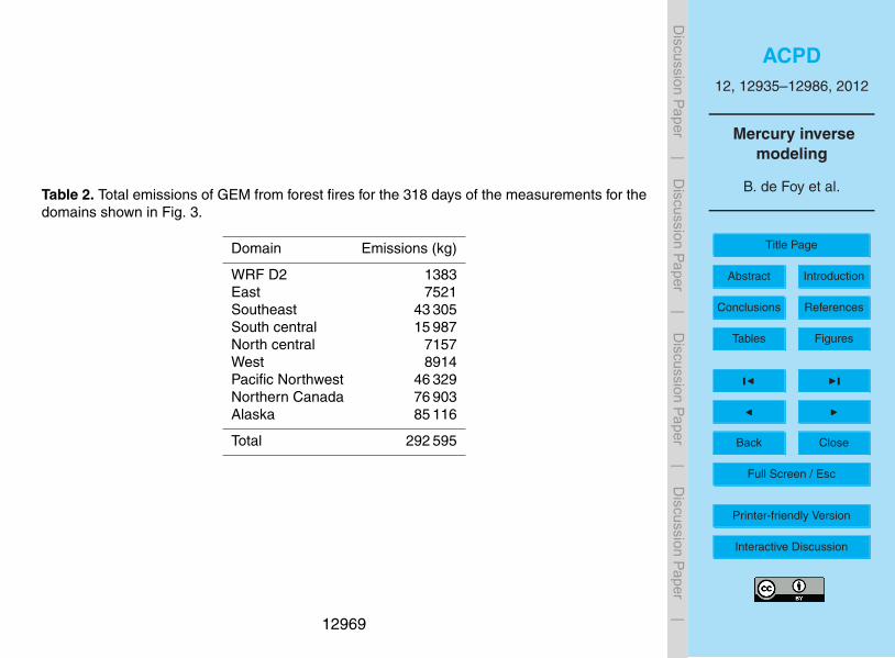
ACPD12, 12935–12986, 2012


B. de Foy et al.

Title Page



Tables Figures

J I

J I

Back Close

Full Screen / Esc



Discussion

Paper

|D

iscussionP

aper|

Discussion

Paper

|D

iscussionP

aper|

Table 2. Total emissions of GEM from forest fires for the 318 days of the measurements for thedomains shown in Fig. 3.

Domain Emissions (kg)

WRF D2 1383East 7521Southeast 43 305South central 15 987North central 7157West 8914Pacific Northwest 46 329Northern Canada 76 903Alaska 85 116

Total 292 595

12969





ACPD12, 12935–12986, 2012


B. de Foy et al.

Title Page



Tables Figures

J I

J I

Back Close

Full Screen / Esc



Discussion

Paper

|D

iscussionP

aper|

Discussion

Paper

|D

iscussionP

aper|

Table 3. Gridded emission totals for domains shown in Fig. 11.

Emissions (kgyr−1) Median Lower-quartile Upper-quartile TRI 2004 GEM NEI 2002 Hg NEI 2002

Local (50 km radius) 984 835 1164 217 71 193South regional 6071 5023 7503 1887 1551 3248Northeast 13 198 10 569 17 194 1510 578 2276Southeast 23 003 19 761 26 391 17 658 6035 25 603West regional 3523 2662 4922 1158 251 1430Southwest 23 770 20 942 27 367 7163 3796 9701Northwest 5761 4331 7346 1582 832 3480

Total 76 310 64 123 91 887 31 176 13 114 45 932

12970





ACPD12, 12935–12986, 2012


B. de Foy et al.

Title Page



Tables Figures

J I

J I

Back Close

Full Screen / Esc



Discussion

Paper

|D

iscussionP

aper|

Discussion

Paper

|D

iscussionP

aper|

Table 4. Scaling factors for forest fires emissions and lake surface emissions shown in Fig. 9.

Domain Median Lower-quartile Upper-quartile

WRF D2 0 0 0East 3.9 3.1 4.5Southeast 1.1 0.6 1.6South central 1.2 0.8 1.6North central 2.6 2.2 3.3West 6.7 3.9 10.1Pacific northwest 0.0 0.0 0.0Northern Canada 0.1 0.0 0.2Alaska 0 0 0

Lake surface 1.9 1.7 2.2

12971





ACPD12, 12935–12986, 2012


B. de Foy et al.

Title Page



Tables Figures

J I

J I

Back Close

Full Screen / Esc



Discussion

Paper

|D

iscussionP

aper|

Discussion

Paper

|D

iscussionP

aper|

Table 5. Contribution of different source groups to the annual average GEM concentration(pgm−3) at the receptor site.

Source group Median Lower-quartile Upper-quartile

Grids Local (50 km radius) 63.8 54.1 71.7South regional 29.7 25.8 35.9Northeast 26.6 21.0 33.6Southeast 16.2 13.1 19.4West regional 15.8 11.5 21.7Southwest 22.9 19.0 25.0Northwest 10.6 8.2 14.2

Total Grid 187.9 177.3 202.2

Fires WRF d2 0.0 0.0 0.0East 46.2 36.6 52.8Southeast 11.6 6.2 16.5South central 8.2 5.6 10.7North central 10.6 8.8 13.4West 5.5 3.2 8.3Pacific northwest 0.0 0.0 0.4Northern Canada 4.2 0.7 6.3Alaska 0.0 0.0 0.0

Total Fires 86.2 61.0 108.3

Lake surface 61.2 53.8 71.5Local and regional background 490.0 480.0 510.0Global background 1500.0 1500.0 1500.0Unaccounted for in model 149.2 144.3 150.4

Inverted timeseries 2330.3 2323.9 2341.1Measurements 2479.5 2468.2 2491.4

12972





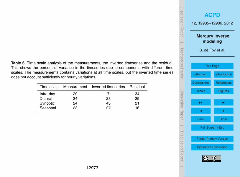
ACPD12, 12935–12986, 2012


B. de Foy et al.

Title Page



Tables Figures

J I

J I

Back Close

Full Screen / Esc



Discussion

Paper

|D

iscussionP

aper|

Discussion

Paper

|D

iscussionP

aper|

Table 6. Time scale analysis of the measurements, the inverted timeseries and the residual.This shows the percent of variance in the timeseries due to components with different timescales. The measurements contains variations at all time scales, but the inverted time seriesdoes not account sufficiently for hourly variations.

Time scale Measurement Inverted timeseries Residual

Intra-day 29 7 34Diurnal 24 23 29Synoptic 24 43 21Seasonal 23 27 16

12973





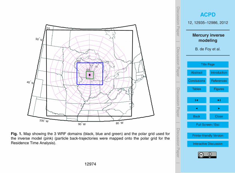
ACPD12, 12935–12986, 2012


B. de Foy et al.

Title Page



Tables Figures

J I

J I

Back Close

Full Screen / Esc



Discussion

Paper

|D

iscussionP

aper|

Discussion

Paper

|D

iscussionP

aper|

D1

D2

D3

100° W 90° W 80° W

40 ° N

50 ° N

Fig. 1. Map showing the 3 WRF domains (black, blue and green) and the polar grid used forthe inverse model (pink) (particle back-trajectories were mapped onto the polar grid for theResidence Time Analysis).

12974





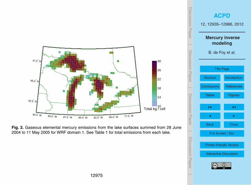
ACPD12, 12935–12986, 2012


B. de Foy et al.

Title Page



Tables Figures

J I

J I

Back Close

Full Screen / Esc



Discussion

Paper

|D

iscussionP

aper|

Discussion

Paper

|D

iscussionP

aper|

10

14

18

22

26

30

Total kg / cell

92.5° W 90.0° W 87.5° W 85.0° W 82.5° W 80.0° W 77.5° W

42.5° N

45.0° N

47.5° N

Fig. 2. Gaseous elemental mercury emissions from the lake surfaces summed from 28 June2004 to 11 May 2005 for WRF domain 1. See Table 1 for total emissions from each lake.

12975





ACPD12, 12935–12986, 2012


B. de Foy et al.

Title Page



Tables Figures

J I

J I

Back Close

Full Screen / Esc



Discussion

Paper

|D

iscussionP

aper|

Discussion

Paper

|D

iscussionP

aper|

0

100

200

300

400

500

Total kg / cell

AK

PNW

W

NCA

NCR

SCR

SE

E

D2

160 ° W

140 ° W

120° W 100° W

80° W

60° W

40 ° N

60 ° N

Fig. 3. Forest fires emissions from 28 June 2004 to 11 May 2005, showing the different domainsused: Alaska (AK), Northern Canada (NCA), pacific northwest (PNW), west (W), north central(NCR), south central (SCR), east (E), southeast (SE). Note that the east domain does notinclude WRF domain 2 (D2) which is calculated separately. The maximum emissions in a cellis 7224 kg, in Alaska. See Table 2 for total emissions by domain.

12976





ACPD12, 12935–12986, 2012


B. de Foy et al.

Title Page



Tables Figures

J I

J I

Back Close

Full Screen / Esc



Discussion

Paper

|D

iscussionP

aper|

Discussion

Paper

|D

iscussionP

aper|

06/25 07/15 08/04 08/24 09/13 10/03 10/23 11/12 12/02 12/22 01/11 01/31 02/20 03/12 04/01 04/21 05/11

5

10

15

20

Gas

eous

Ele

men

tal M

ercu

ry (

ng/m

3 )

Fig. 4. Time series of elemental gaseous mercury in Milwaukee from 28 June 2004 to 11 May2005. This shows a combination of variations across time scales from short peaks lasting hoursor less to longer events lasting days or even weeks.

12977





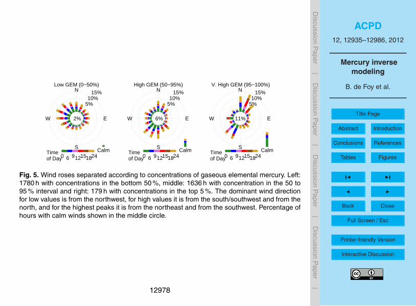
ACPD12, 12935–12986, 2012


B. de Foy et al.

Title Page



Tables Figures

J I

J I

Back Close

Full Screen / Esc



Discussion

Paper

|D

iscussionP

aper|

Discussion

Paper

|D

iscussionP

aper|

5%10%

15%N

E

S

W 2%

Calm 0 6 912151824

Timeof Day

Low GEM (0−50%)

5%10%

15%N

E

S

W 6%

Calm 0 6 912151824

Timeof Day

High GEM (50−95%)

5%10%

15%N

E

S

W 11%

Calm 0 6 912151824

Timeof Day

V. High GEM (95−100%)

Fig. 5. Wind roses separated according to concentrations of gaseous elemental mercury. Left:1780 h with concentrations in the bottom 50 %, middle: 1636 h with concentration in the 50 to95 % interval and right: 179 h with concentrations in the top 5 %. The dominant wind directionfor low values is from the northwest, for high values it is from the south/southwest and from thenorth, and for the highest peaks it is from the northeast and from the southwest. Percentage ofhours with calm winds shown in the middle circle.

12978





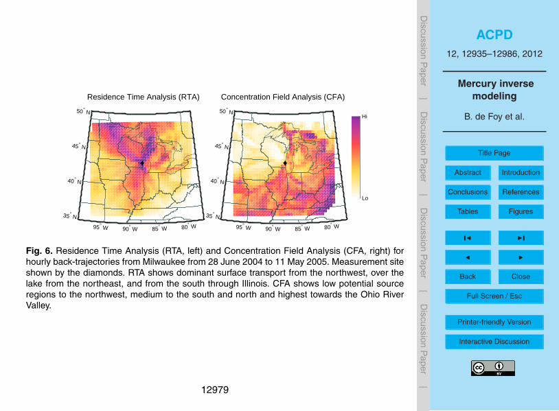
ACPD12, 12935–12986, 2012


B. de Foy et al.

Title Page



Tables Figures

J I

J I

Back Close

Full Screen / Esc



Discussion

Paper

|D

iscussionP

aper|

Discussion

Paper

|D

iscussionP

aper|

95° W 90° W 85° W 80° W

35° N

40° N

45° N

50° N

95° W 90° W 85° W 80° W

35° N

40° N

45° N

50° N

Lo

Hi

Residence Time Analysis (RTA) Concentration Field Analysis (CFA)

Fig. 6. Residence Time Analysis (RTA, left) and Concentration Field Analysis (CFA, right) forhourly back-trajectories from Milwaukee from 28 June 2004 to 11 May 2005. Measurement siteshown by the diamonds. RTA shows dominant surface transport from the northwest, over thelake from the northeast, and from the south through Illinois. CFA shows low potential sourceregions to the northwest, medium to the south and north and highest towards the Ohio RiverValley.

12979





ACPD12, 12935–12986, 2012


B. de Foy et al.

Title Page



Tables Figures

J I

J I

Back Close

Full Screen / Esc



Discussion

Paper

|D

iscussionP

aper|

Discussion

Paper

|D

iscussionP

aper|

0.0

0.1

0.2

0.3

0.4

0.5

0.6

0.7

0.8

EmissionFraction

100° W 90° W 80° W

40° N

50° N

Fig. 7. Map of emissions from the inverse model using synthetic simulations from a location(+) 213 km northwest of the receptor site (diamond). Units are fraction of the synthetic release.Extent of the back-trajectory grid used for the inversion shown in pink.

12980





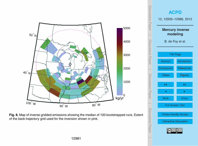
ACPD12, 12935–12986, 2012


B. de Foy et al.

Title Page



Tables Figures

J I

J I

Back Close

Full Screen / Esc



Discussion

Paper

|D

iscussionP

aper|

Discussion

Paper

|D

iscussionP

aper|

0

1000

2000

3000

4000

5000

kg/yr 100° W

90° W 80° W

40° N

50° N

Fig. 8. Map of inverse gridded emissions showing the median of 100 bootstrapped runs. Extentof the back-trajectory grid used for the inversion shown in pink.

12981





ACPD12, 12935–12986, 2012


B. de Foy et al.

Title Page



Tables Figures

J I

J I

Back Close

Full Screen / Esc



Discussion

Paper

|D

iscussionP

aper|

Discussion

Paper

|D

iscussionP

aper|

0 1 2 3 4 5 60

20

40

60

Lakes

0 1 2 3 4 5 6

East

0 1 2 3 4 5 6

Southeast

0 1 2 3 4 5 9

N. Central

0 1 2 3 4 5 70

20

40

60

S. Central

0 4 8 12 16 22

West

0 0.1 0.2 0.3 0.4 1

N. Canada

0 0.04 0.08 0.12 0.16 1

Pacific NW

Inverse Emissions Scaling Factor for Lake Surface and Forest Fire Sources

Fre

quen

cy (

%)

Fig. 9. Histograms of inverse emissions scaling factors for emissions from the Great Lakes andfrom forest fires by domain. See Fig. 2 for map of lake emissions and Fig. 3 for map of forestfire emissions. (Note that factors for Alaska and WRF D2 are always 0.)

12982





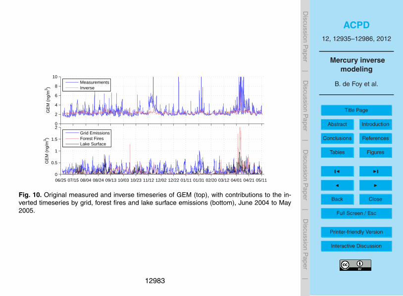
ACPD12, 12935–12986, 2012


B. de Foy et al.

Title Page



Tables Figures

J I

J I

Back Close

Full Screen / Esc



Discussion

Paper

|D

iscussionP

aper|

Discussion

Paper

|D

iscussionP

aper|

0

2

4

6

8

10

GE

M (

ng/m

3 )

MeasurementsInverse

06/25 07/15 08/04 08/24 09/13 10/03 10/23 11/12 12/02 12/22 01/11 01/31 02/20 03/12 04/01 04/21 05/110

0.5

1

1.5

2

GE

M (

ng/m

3 )

Grid EmissionsForest FiresLake Surface

Fig. 10. Original measured and inverse timeseries of GEM (top), with contributions to the in-verted timeseries by grid, forest fires and lake surface emissions (bottom), June 2004 to May2005.

12983





ACPD12, 12935–12986, 2012


B. de Foy et al.

Title Page



Tables Figures

J I

J I

Back Close

Full Screen / Esc



Discussion

Paper

|D

iscussionP

aper|

Discussion

Paper

|D

iscussionP

aper|

NENW

SW SE 100° W 95° W 90° W 85° W 80° W

35° N

40° N

45° N

50° N

W Regional

S Regional

90° W 88° W 86° W

42° N

44° N

0

2

3

5

6

8

pg/m3

Local

88.5° W 88.0° W 87.5° W

43.0° N

43.5° N

Full Grid (1024 km Radius) 290 km RadiusMedian Concentration at the Measurement Site due to Cell Emissions

50 km Radius

Fig. 11. Map of impacts at the receptor site. Color indicates the average GEM concentrationat the measurement site due to emissions in that cell. Domain names and boundaries used inTables 3 and 5 shown in pink.

12984





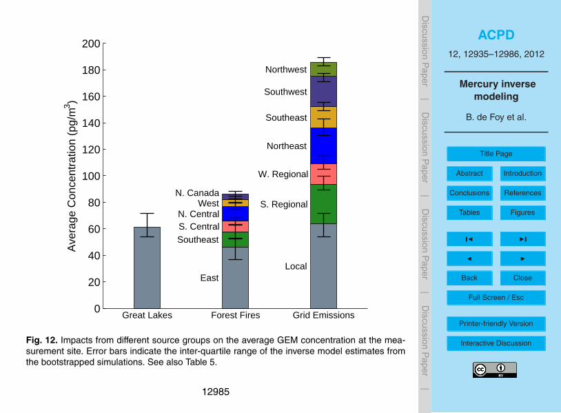
ACPD12, 12935–12986, 2012


B. de Foy et al.

Title Page



Tables Figures

J I

J I

Back Close

Full Screen / Esc



Discussion

Paper

|D

iscussionP

aper|

Discussion

Paper

|D

iscussionP

aper|

0

20

40

60

80

100

120

140

160

180

200

Great Lakes

East

SoutheastS. CentralN. Central

WestN. Canada

Forest Fires

Local

S. Regional

W. Regional

Northeast

Southeast

Southwest

Northwest

Grid Emissions

Ave

rage

Con

cent

ratio

n (p

g/m

3 )

Fig. 12. Impacts from different source groups on the average GEM concentration at the mea-surement site. Error bars indicate the inter-quartile range of the inverse model estimates fromthe bootstrapped simulations. See also Table 5.

12985





ACPD12, 12935–12986, 2012


B. de Foy et al.

Title Page



Tables Figures

J I

J I

Back Close

Full Screen / Esc



Discussion

Paper

|D

iscussionP

aper|

Discussion

Paper

|D

iscussionP

aper|

0

446

892

1339

1785

2231

kg/yr 100° W 95° W 90° W 85° W 80° W

35° N

40° N

45° N

50° N

0

161

322

483

644

805

kg/yr 100° W 95° W 90° W 85° W 80° W

35° N

40° N

45° N

50° N

0

660

1321

1981

2642

3302

kg/yr 100° W 95° W 90° W 85° W 80° W

35° N

40° N

45° N

50° N

TRI Hg NEI GEM NEI Hg

Fig. 13. Map of inventories of all mercury compounds from the Toxic Release Inventory (left),of GEM from the 2002 National Emissions Inventory (middle) and all mercury compounds fromthe 2002 NEI (right). Extent of the back-trajectory grid used for the inversion shown in pink.

12986





Mercury inverse modeling

Documents

Transcript of Mercury inverse modeling