Optimal Inverse Littlewood-Offord theorems
23
arXiv:1004.3967v2 [math.CO] 16 Jan 2011 OPTIMAL INVERSE LITTLEWOOD-OFFORD THEOREMS HOI NGUYEN AND VAN VU Abstract. Let ηi ,i =1,...,n be iid Bernoulli random variables, taking values ±1 with probability 1 2 . Given a multiset V of n integers v1,...,vn, we define the concentration probability as ρ(V ) := sup x P(v1η1 + ...vnηn = x). A classical result of Littlewood-Offord and Erd˝ os from the 1940s asserts that, if the vi are non-zero, then ρ(V ) is O(n −1/2 ). Since then, many researchers have obtained improved bounds by assuming various extra restrictions on V . About 5 years ago, motivated by problems concerning random matrices, Tao and Vu introduced the Inverse Littlewood-Offord problem. In the inverse problem, one would like to characterize the set V , given that ρ(V ) is relatively large. In this paper, we introduce a new method to attack the inverse problem. As an ap- plication, we strengthen the previous result of Tao and Vu, obtaining an optimal char- acterization for V . This immediately implies several classical theorems, such as those of S´ark¨ozy-Szemer´ edi and Hal´ asz. The method also applies to the continuous setting and leads to a simple proof for the β-net theorem of Tao and Vu, which plays a key role in their recent studies of random matrices. All results extend to the general case when V is a subset of an abelian torsion-free group, and ηi are independent variables satisfying some weak conditions. 1. Introduction 1.1. The Forward Littlewood-Offord problem. Let η i ,i =1,...,n be iid Bernoulli random variables, taking values ±1 with probability 1 2 . Given a multiset V of n integers v 1 ,...,v n , we define the random walk S with steps in V to be the random variable S := ∑ n i=1 v i η i . The concentration probability is defined to be ρ(V ) := sup x P(S = x). Motivated by their study of random polynomials in the 1940s, Littlewood and Offord [7] raised the question of bounding ρ(V ). (We call this the forward Littlewood-Offord problem, in contrast with the inverse Littlewood-Offord problem discussed in the next section.) They 2000 Mathematics Subject Classification. 11B25. Key words and phrases. inverse Littlewood-Offord problem, concentration probability, generalized arith- metic progression. Both authors are supported by research grants DMS-0901216 and AFOSAR-FA-9550-09-1-0167. 1
-
Upload
independent -
Category
Documents
-
view
1 -
download
0
Transcript of Optimal Inverse Littlewood-Offord theorems
arX
iv:1
004.
3967
v2 [
mat
h.C
O]
16
Jan
2011
OPTIMAL INVERSE LITTLEWOOD-OFFORD THEOREMS
HOI NGUYEN AND VAN VU
Abstract. Let ηi, i = 1, . . . , n be iid Bernoulli random variables, taking values ±1 withprobability 1
2. Given a multiset V of n integers v1, . . . , vn, we define the concentration
probability as
ρ(V ) := supx
P(v1η1 + . . . vnηn = x).
A classical result of Littlewood-Offord and Erdos from the 1940s asserts that, if the viare non-zero, then ρ(V ) is O(n−1/2). Since then, many researchers have obtained improvedbounds by assuming various extra restrictions on V .
About 5 years ago, motivated by problems concerning random matrices, Tao and Vuintroduced the Inverse Littlewood-Offord problem. In the inverse problem, one would liketo characterize the set V , given that ρ(V ) is relatively large.
In this paper, we introduce a new method to attack the inverse problem. As an ap-plication, we strengthen the previous result of Tao and Vu, obtaining an optimal char-acterization for V . This immediately implies several classical theorems, such as those ofSarkozy-Szemeredi and Halasz.
The method also applies to the continuous setting and leads to a simple proof for theβ-net theorem of Tao and Vu, which plays a key role in their recent studies of randommatrices.
All results extend to the general case when V is a subset of an abelian torsion-freegroup, and ηi are independent variables satisfying some weak conditions.
1. Introduction
1.1. The Forward Littlewood-Offord problem. Let ηi, i = 1, . . . , n be iid Bernoullirandom variables, taking values ±1 with probability 1
2 . Given a multiset V of n integersv1, . . . , vn, we define the random walk S with steps in V to be the random variable S :=∑n
i=1 viηi. The concentration probability is defined to be
ρ(V ) := supx
P(S = x).
Motivated by their study of random polynomials in the 1940s, Littlewood and Offord [7]raised the question of bounding ρ(V ). (We call this the forward Littlewood-Offord problem,in contrast with the inverse Littlewood-Offord problem discussed in the next section.) They
2000 Mathematics Subject Classification. 11B25.Key words and phrases. inverse Littlewood-Offord problem, concentration probability, generalized arith-
metic progression.Both authors are supported by research grants DMS-0901216 and AFOSAR-FA-9550-09-1-0167.
1
2 HOI NGUYEN AND VAN VU
showed that ρ(V ) = O(n−1/2 log n). Shortly after the Littlewood-Offord paper, Erdos [1]gave a beautiful combinatorial proof of the refinement
ρ(V ) ≤( nn/2
)
2n= O(n−1/2). (1)
Erdos’ result is sharp, as demonstrated by V = 1, . . . , 1.
Notation. Here and later, asymptotic notations, such as O,Ω,Θ, and so forth, are usedunder the assumption that n → ∞. A notation such as OC(.) emphasizes that the hiddenconstant in O depends on C. If a = Ω(b), we write b ≪ a or a ≫ b. All logarithms have anatural base, if not specified otherwise.
The results of Littlewood-Offord and Erdos are classics in combinatorics and have generatedan impressive wave of research, particularly from the early 1960s to the late 1980s.
One direction of research was to generalize Erdos’ result to other groups. For example, in1966 and 1970, Kleitman extended Erdos’ result to complex numbers and normed vectors,respectively. Several results in this direction can be found in [3, 5].
Another direction was motivated by the observation that (1) can be improved significantlyby making additional assumptions about V . The first such result was discovered by Erdosand Moser [2], who showed that if vi are distinct, then ρ(V ) = O(n−3/2 log n). Theyconjectured that the logarithmic term is not necessary, and this was confirmed by Sarkozyand Szemeredi [12].
Theorem 1.2. Let V be a set of n different integers, then
ρ(V ) = O(n−3/2).
In [4] (see also in [23]), Halasz proved very general theorems that imply Theorem 1.2 andmany others. One of his results can be formulated as follows.
Theorem 1.3. Let l be a fixed integer and Rl be the number of solutions of the equationvi1 + · · ·+ vil = vj1 + · · ·+ vjl. Then
ρ(V ) = O(n−2l− 12Rl).
It is easy to see, by setting l = 1, that Theorem 1.3 implies Theorem 1.2.
Another famous result in this area is that of Stanley [13], which, solving a conjecture ofErdos and Moser, shows when ρ(V ) attains its maximum under the assumption that the viare different.
Theorem 1.4. Let n be odd and V0 := −⌊n/2⌋, . . . , ⌊n/2⌋. Then
ρ(V ) ≤ ρ(V0).
INVERSE LITTLEWOOD-OFFORD PROBLEM 3
A similar result holds for the case of n being even [13]. Stanley’s proof of Theorem 1.4 usedsophisticated machinery from algebraic geometry, particularly the hard Lefschetz theorem.A few years later, a more elementary proof was given by Proctor [9]. This proof also hasan algebraic nature, involving the representation of the Lie algebra sl(2,C). As far as weknow, there is no purely combinatorial proof.
It is natural to ask for the actual value of ρ(V0). From Theorem 1.2, one would guess (underthe assumption that the elements of V are different) that
ρ(V0) = (C0 + o(1))n−3/2
for some constant C0 > 0. However, the algebraic proofs do not give the value of C0. Infact, it is not obvious that limn→∞ n3/2ρ(V0) exists.
Assuming that C0 exists for a moment, one would next wonder if V0 is a stable maximizer.In other words, if some other set V ′
0 has ρ(V ′0) close to C0n
−3/2, then should V ′0 (possibly
after a normalization) be ”close” to V0 ? (Note that ρ is invariant under dilation, so anormalization would be necessary.)
1.5. The inverse Littlewood-Offord problem. Motivated by inverse theorems fromadditive combinatorics (see [23, Chapter 5]) and a variant for random sums in [20, Theorem5.2], Tao and the second author [18] brought a different view to the problem. Instead oftrying to improve the bound further by imposing new assumptions (as done in the forwardproblems), they tried to provide the complete picture by finding the underlying reason asto why the concentration probability is large (say, polynomial in n).
Note that the (multi)-set V has 2n subsums, and ρ(V ) ≥ n−C means that at least 2n
nC ofthese take the same value. This observation suggests that the set should have a very strongadditive structure. To determine this structure, we first discuss a few examples of V , whereρ(V ) is large. For a set A, we denote the set a1 + · · · + al|ai ∈ A by lA.
Example 1.6. Let I = [−N,N ] and v1, . . . , vn be elements of I. Because S ∈ nI, by thepigeon-hole principle, ρ(V ) ≥ 1
|nI| = Ω( 1nN ). In fact, a short consideration yields a better
bound. Note that, with a probability of least .99, we have S ∈ 10√nI. Thus, again by the
pigeon-hole principle, we have ρ(V ) = Ω( 1√nN
). If we set N = nC−1/2 for some constant
C ≥ 1/2, then
ρ(V ) = Ω(1
nC). (2)
The next, and more general, construction comes from additive combinatorics. A very im-portant concept in this area is that of generalized arithmetic progressions (GAPs). A set Qis a GAP of rank r if it can be expressed as in the form
Q = a0 + x1a1 + · · · + xrar|Mi ≤ xi ≤ M ′i for all 1 ≤ i ≤ r
for some a0, . . . , ar, M1, . . . ,Mr, and M ′1, . . . ,M
′r.
4 HOI NGUYEN AND VAN VU
It is convenient to think of Q as the image of an integer box B := (x1, . . . , xr) ∈ Zr|Mi ≤mi ≤ M ′
i under the linear map
Φ : (x1, . . . , xr) 7→ a0 + x1a1 + · · ·+ xrar.
The numbers ai are the generators of P , the numbers Mi and M ′i are the dimensions of
P , and Vol(Q) := |B| is the volume of B. We say that Q is proper if this map is one-to-oneor, equivalently, if |Q| = Vol(Q). For non-proper GAPs, we, of course, have |Q| < Vol(Q).If −Mi = M ′
i for all i ≥ 1 and a0 = 0, we say that Q is symmetric.
Example 1.7. Let Q be a proper symmetric GAP of rank r and volume N . Let v1, . . . , vnbe (not necessarily distinct) elements of P . The random variable S =
∑ni=1 viηi takes values
in the GAP nP . Because |nP | ≤ Vol(nB) = nrN , the pigeon-hole principle implies thatρ(V ) ≥ Ω( 1
nrN ). In fact, using the same idea as in the previous example, one can improve
the bound to Ω( 1nr/2N
). If we set N = nC−r/2 for some constant C ≥ r/2, then
ρ(V ) = Ω(1
nC). (3)
The examples above show that, if the elements of V belong to a proper GAP with a smallrank and small cardinality, then ρ(V ) is large. A few years ago, Tao and the second author[18] showed that this is essentially the only reason:
Theorem 1.8 (Weak inverse theorem). [18] Let C, ǫ > 0 be arbitrary constants. Thereare constants r and C ′ depending on C and ǫ such that the following holds. Assume thatV = v1, . . . , vn is a multiset of integers satisfying ρ(V ) ≥ n−C. Then, there is a proper
symmetric GAP Q with a rank of at most r and a volume of at most nC′
that contains allbut at most n1−ǫ elements of V (counting multiplicity).
Remark 1.9. The presence of a small set of exceptional elements is not completely avoidable.For instance, one can add o(log n) completely arbitrary elements to V and, at worst, onlydecrease ρ(V ) by a factor of n−o(1). Nonetheless, we expect the number of such elementsto be less than what is given by the results here.
The reason we call Theorem 1.8 weak is that C ′ is not optimal. In particular, it is far fromreflecting the relations in (2) and (3). In a later paper [16], Tao and the second authorrefined the approach to obtain the following stronger result.
Theorem 1.10 (Strong inverse theorem). [16] Let C and 1 > ε be positive constants.Assume that
ρ(V ) ≥ n−C .
Then, there exists a proper symmetric GAP Q of rank r = OC,ε(1) that contains all butOr(n
1−ε) elements of V (counting multiplicity), where
|Q| = OC,ε(nC− r
2+ε).
The bound on |Q| matches Example 1.7, up to the nǫ term. However, this error term seemsto be the limit of the approach. The proofs of Theorems 1.8 and 1.10 rely on a replacementargument and various lemmas about random walks and GAPs.
INVERSE LITTLEWOOD-OFFORD PROBLEM 5
Let us now consider an application of Theorem 1.10. Note that Theorem 1.10 enables usto make very precise counting arguments. Assume that we would like to count the numberof (multi)sets V of integers with max |vi| ≤ N = nO(1) such that ρ(V ) ≥ ρ := n−C .
Fix d ≥ 1, and fix 1 a GAP Q with rank r and volume |Q| = nC− r2 . The dominating term
in the calculation will be the number of multi-subsets of size n of Q, which is
|Q|n = n(C− r2+ǫ)n ≤ nCnn−n
2+ǫn = ρ−nn−n( 1
2−ǫ). (4)
Motivated by questions from random matrix theory, Tao and the second author obtainedthe following continuous analogue of this result.
Definition 1.11 (Small ball probability). Let z be a real random variable, and let V =v1, . . . , vn be a multiset in Rd. For any r > 0, we define the small ball probability as
ρr,z(V ) := supx∈Rd
P(v1z1 + . . . vnzn ∈ B(x, r)),
where z1, . . . , zn are iid copies of z, and B(x, r) denotes the closed disk of radius r centeredat x in Rd.
Let n be a positive integer and β, ρ be positive numbers that may depend on n. Let Sn,β,ρ
be the collection of all multisets V = v1, . . . , vn, vi ∈ R2 such that∑n
i=1 ‖vi‖2 = 1 andρβ,η(V ) ≥ ρ, where η has a Bernoulli distribution.
Theorem 1.12 (The β-net Theorem). [21] Let 0 < ǫ ≤ 1/3 and C > 0 be constants. Then,for all sufficiently large n and β ≥ exp(−nǫ) and ρ ≥ n−C , there is a set S ⊂ (R2)n of sizeat most
ρ−nn−n( 12−ǫ) + exp(o(n))
such that for any V = v1, . . . , vn ∈ Sn,β,ρ, there is some V ′ = (v′1, . . . , v′n) ∈ S such that
‖vi − v′i‖2 ≤ β for all i.
The theorem looks a bit cleaner if we use C instead of R2 (as in [21]). However, we preferthe current form, because it is more suitable for generalization. The set S is usually referredto as a β-net of Sn,β,ρ.
Theorem 1.12 is at the heart of establishing the Circular Law conjecture in random matrixtheory (see [21, 17]). It also plays an important role in the study of the condition numberof randomly perturbed matrices (see [22]). Its proof in [21] is quite technical and occupiesthe bulk of that paper.
1A more detailed version of Theorems 1.8 and 1.10 tells us that there are not too many ways to choosethe generators of Q. In particular, if N = nO(1), the number of ways to fix these is negligible compared tothe main term.
6 HOI NGUYEN AND VAN VU
However, given the above discussion, one might expect to obtain Theorem 1.12 as a simplecorollary of a continuous analogue of Theorem 1.10. However, the arguments in [21] havenot yet provided such an inverse theorem (although they did provide a sufficient amountof information about the set S to make an estimate possible). The paper [10] by Rudelsonand Vershynin also contains a characterization of the set S, but their characterization hasa somewhat different spirit than those discussed in this paper.
2. A new approach and new results
In this paper, we introduce a new approach to the inverse theorem. The core of this newapproach is a (long-range) variant of Freiman’s famous inverse theorem.
This new approach seems powerful. First, it enables us to remove the error term nǫ inTheorem 1.10, resulting in an optimal inverse theorem.
Theorem 2.1 (Optimal inverse Littlewood-Offord theorem, discrete case). Let ε < 1 andC be positive constants. Assume that
ρ(V ) ≥ n−C .
Then, there exists a proper symmetric GAP Q of rank r = OC,ε(1) that contains all but atmost εn elements of V (counting multiplicity), where
|Q| = OC,ε(ρ(V )−1n− r2 ).
This immediately implies several forward theorems, such as Theorems 1.2 and 1.3. Forexample, we can prove Theorem 1.2 as follows.
Proof. (of Theorem 1.2) Assume, for contradiction, that there is a set V of n distinct
numbers such that ρ(V ) ≥ c1n−3/2 for some large constant c1 to be chosen. Set ε = .1, C =
3/2. By Theorem 2.1, there is a GAP Q of rank r and size OC,ǫ(1c1nC− r
2 ) that contains at
least .9n elements from V . This implies |Q| ≥ .9n. By setting c1 to be sufficiently large andusing the fact that C = 3/2 and r ≥ 1, we can guarantee that |Q| ≤ .8n, a contradiction.
Theorem 1.3 can be proved in a similar manner with the details left as an exercise.
Similar to [16, 18], our method and results can be extended (rather automatically) to muchmore general settings.
General V . Instead of taking V to be a subset of Z, we can take it to be a subset of anyabelian torsion-free group G (thanks to Freiman isomorphism, see Section 4). We can alsoreplace Z by the finite field Fp, where p is any sufficiently large prime. (In fact, the firststep in our proof is to embed V into Fp.)
General η. We can replace the Bernoulli random variables by independent random variablesηi satisfying the following condition. There is a constant c > 0 and an infinite sequence ofprimes p such that for any p in the sequence, any (multi)-subset V of size n of Fp and anyt ∈ Fp
INVERSE LITTLEWOOD-OFFORD PROBLEM 7
n∏
i=1
|Eep(ηivit)| ≤ exp(−cn∑
i=1
‖vitp‖2) (5)
where ‖x‖ denotes the distance from x to the closest integer (we view the elements of Fp
as integers between 0 and p− 1) and ep(x) := exp(2π√−1x/p).
Example 2.2. (Lazy random walks) Given a parameter 0 < µ ≤ 1, let ηµi be iid copies of arandom variable ηµ, where ηµ = 1 or −1 with probability µ/2, and ηµ = 0 with probability1− µ. The sum
Sµ(V ) :=n∑
i=1
ηiµvi,
can be viewed as a lazy random walk with steps in V . A simple calculation shows
Eep(ηx) = (1− µ) + µ cos2πx
p.
It is easy to show that there is a constant c > 0 depending on µ such that
|(1 − µ) + µ cos2πx
p| ≤ exp(−c‖x
p‖2).
Example 2.3. (µ-bounded variables) It suffices to assume that there is some constant 0 <µ ≤ 1 such that for all i
|Eep(ηix)| ≤ (1− µ) + µ cos2πx
p. (6)
Theorem 2.4. The conclusion of Theorem 2.1 holds for the case when V is a multi-subsetof an arbitrary torsion-free abelian group G and ηi, 1 ≤ i ≤ n are independent randomvariables satisfying (5).
In some applications, we might need a version of Theorem 2.1 with a smaller number ofexceptional elements. By slightly modifying the proof presented in Section 5, we can provethe following result.
Theorem 2.5. Let ε < 1 and C be positive constants. Assume that
ρ(V ) ≥ n−C .
Then, for any nǫ ≤ n′ ≤ n, there exists a proper symmetric GAP Q of rank r = Oǫ,C(1)that contains all but n′ elements of V (counting multiplicity), where
|Q| = OC,ǫ(ρ−1/n′r/2).
8 HOI NGUYEN AND VAN VU
Remark 2.6. In an upcoming paper [8], we are able to address the unresolved issues con-cerning Theorem 1.4 by following the method used to prove Theorem 2.1. We prove that
ρ(V0) = (√
24π + o(1))n−3/2. More important, we obtain a stable version of Theorem 1.4,
which shows that, if ρ(V ) is close to (√
24/π + o(1))n−3/2, then V is ”close” to V0. As abyproduct, we obtain the first non-algebraic proof for the asymptotic version of the Stanleytheorem.
We now turn to the continuous setting. In this part, we consider a real random variable zsuch that there exists a constant Cz such that
P(1 ≤ |z1 − z2| ≤ Cz) ≥ 1/2, (7)
where z1, z2 are iid copies of z. We note that Bernoulli random variables are clearly ofthis type. (Also, the interested reader may find (7) more general than the condition of theκ-controlled second moment defined in [21] and the condition of bounded third moment in[10].) In the statement above, Cz is not uniquely defined. In what follows, we will take thesmallest value of Cz.
We say that a vector v ∈ Rd is δ-close to a set Q ⊂ Rd if there exists a vector q ∈ Q suchthat ‖v − q‖2 ≤ δ. A set X is δ-close to a set Q if every element of X is δ-close to Q. Theanalogue of Example 1.7 is the following.
Example 2.7. Let Q be a proper symmetric GAP of rank r and volume N in Rd. Letv1, . . . , vn be (not necessarily distinct) vectors that are O(βn−1/2)-close to Q. If we set
|Q| = nC− r2 for some constant C ≥ r/2, then
ρβ,η(V ) = Ω(1
nC). (8)
Thus, one would expect that, if ρβ,z(V ) is large, then (most of) V is O(βn−1/2)-close to aGAP with a small volume. Confirming this intuition, we obtain the following continuousanalogue of Theorem 2.1.
Theorem 2.8 (Optimal inverse Littlewood-Offord theorem, continuous case). Let δ, C > 0be arbitrary constants and β > 0 be a parameter that may depend on n. Suppose thatV = v1, . . . , vn is a (multi-) subset of Rd such that
∑ni=1 ‖vi‖22 = 1 and that V has large
small ball probability
ρ := ρβ,z(V ) ≥ n−C ,
where z is a real random variable satisfying (7). Then, there exists a proper symmetric GAPQ of rank d ≤ r = O(1) so that all but at most δn elements of V (counting multiplicity) are
O(β lognn1/2 )-close to Q, where
|Q| = O(ρ−1δ(−r+d)/2n(−r+d)/2).
The theorem is optimal in the sense that the exponent (−r+ d)/2 of n cannot generally beimproved (see Appendix B for more details).
INVERSE LITTLEWOOD-OFFORD PROBLEM 9
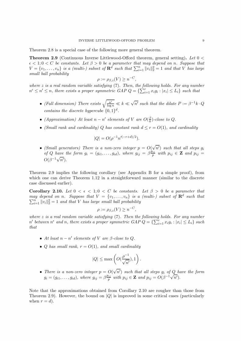
Theorem 2.8 is a special case of the following more general theorem.
Theorem 2.9 (Continuous Inverse Littlewood-Offord theorem, general setting). Let 0 <ǫ < 1; 0 < C be constants. Let β > 0 be a parameter that may depend on n. Suppose thatV = v1, . . . , vn is a (multi-) subset of Rd such that
∑ni=1 ‖vi‖22 = 1 and that V has large
small ball probabilityρ := ρβ,z(V ) ≥ n−C ,
where z is a real random variable satisfying (7). Then, the following holds. For any numbernǫ ≤ n′ ≤ n, there exists a proper symmetric GAP Q = ∑r
i=1 xigi : |xi| ≤ Li such that
• (Full dimension) There exists√
n′
logn ≪ k ≪√n′ such that the dilate P := β−1k ·Q
contains the discrete hypercube 0, 1d.
• (Approximation) At least n− n′ elements of V are O(βk )-close to Q.
• (Small rank and cardinality) Q has constant rank d ≤ r = O(1), and cardinality
|Q| = O(ρ−1n′(−r+d)/2).
• (Small generators) There is a non-zero integer p = O(√n′) such that all steps gi
of Q have the form gi = (gi1, . . . , gid), where gij = βpijp with pij ∈ Z and pij =
O(β−1√n′).
Theorem 2.9 implies the following corollary (see Appendix B for a simple proof), fromwhich one can derive Theorem 1.12 in a straightforward manner (similar to the discretecase discussed earlier).
Corollary 2.10. Let 0 < ǫ < 1; 0 < C be constants. Let β > 0 be a parameter thatmay depend on n. Suppose that V = v1, . . . , vn is a (multi-) subset of Rd such that∑n
i=1 ‖vi‖22 = 1 and that V has large small ball probability
ρ := ρβ,z(V ) ≥ n−C ,
where z is a real random variable satisfying (7). Then the following holds. For any numbern′ between nǫ and n, there exists a proper symmetric GAP Q = ∑r
i=1 xigi : |xi| ≤ Li suchthat
• At least n− n′ elements of V are β-close to Q.
• Q has small rank, r = O(1), and small cardinality
|Q| ≤ max
(
O(ρ−1
√n′ ), 1
)
.
• There is a non-zero integer p = O(√n′) such that all steps gi of Q have the form
gi = (gi1, . . . , gid), where gij = βpijp with pij ∈ Z and pij = O(β−1
√n′).
Note that the approximations obtained from Corollary 2.10 are rougher than those fromTheorem 2.9). However, the bound on |Q| is improved in some critical cases (particularlywhen r = d).
10 HOI NGUYEN AND VAN VU
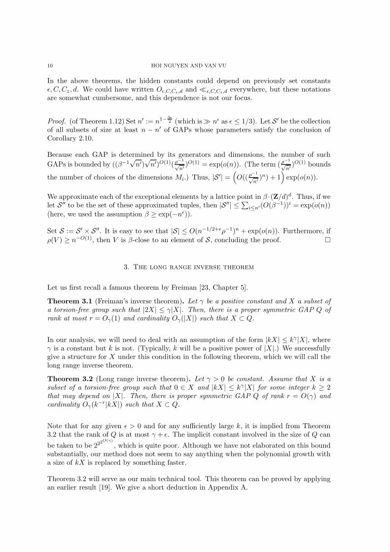
In the above theorems, the hidden constants could depend on previously set constantsǫ, C,Cz , d. We could have written Oǫ,C,Cz,d and ≪ǫ,C,Cz,d everywhere, but these notationsare somewhat cumbersome, and this dependence is not our focus.
Proof. (of Theorem 1.12) Set n′ := n1− 3ǫ2 (which is≫ nǫ as ǫ ≤ 1/3). Let S ′ be the collection
of all subsets of size at least n − n′ of GAPs whose parameters satisfy the conclusion ofCorollary 2.10.
Because each GAP is determined by its generators and dimensions, the number of such
GAPs is bounded by ((β−1√n′)
√n′)O(1)( ρ
−1√n′)O(1) = exp(o(n)). (The term ( ρ
−1√n′)O(1) bounds
the number of choices of the dimensions Mi.) Thus, |S ′| =(
O(( ρ−1
√n′)n) + 1
)
exp(o(n)).
We approximate each of the exceptional elements by a lattice point in β ·(Z/d)d. Thus, if welet S ′′ to be the set of these approximated tuples, then |S ′′| ≤∑i≤n′(O(β−1))i = exp(o(n))
(here, we used the assumption β ≥ exp(−nǫ)).
Set S := S ′ × S ′′. It is easy to see that |S| ≤ O(n−1/2+ǫρ−1)n + exp(o(n)). Furthermore, if
ρ(V ) ≥ n−O(1), then V is β-close to an element of S, concluding the proof.
3. The long range inverse theorem
Let us first recall a famous theorem by Freiman [23, Chapter 5].
Theorem 3.1 (Freiman’s inverse theorem). Let γ be a positive constant and X a subset ofa torsion-free group such that |2X| ≤ γ|X|. Then, there is a proper symmetric GAP Q ofrank at most r = Oγ(1) and cardinality Oγ(|X|) such that X ⊂ Q.
In our analysis, we will need to deal with an assumption of the form |kX| ≤ kγ |X|, whereγ is a constant but k is not. (Typically, k will be a positive power of |X|.) We successfullygive a structure for X under this condition in the following theorem, which we will call thelong range inverse theorem.
Theorem 3.2 (Long range inverse theorem). Let γ > 0 be constant. Assume that X is asubset of a torsion-free group such that 0 ∈ X and |kX| ≤ kγ |X| for some integer k ≥ 2that may depend on |X|. Then, there is proper symmetric GAP Q of rank r = O(γ) andcardinality Oγ(k
−r|kX|) such that X ⊂ Q.
Note that for any given ǫ > 0 and for any sufficiently large k, it is implied from Theorem3.2 that the rank of Q is at most γ + ǫ. The implicit constant involved in the size of Q can
be taken to be 222O(γ)
, which is quite poor. Although we have not elaborated on this boundsubstantially, our method does not seem to say anything when the polynomial growth witha size of kX is replaced by something faster.
Theorem 3.2 will serve as our main technical tool. This theorem can be proved by applyingan earlier result [19]. We give a short deduction in Appendix A.
INVERSE LITTLEWOOD-OFFORD PROBLEM 11
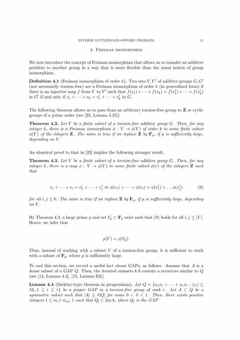
4. Freiman isomorphism
We now introduce the concept of Freiman isomorphism that allows us to transfer an additiveproblem to another group in a way that is more flexible than the usual notion of groupisomorphism.
Definition 4.1 (Freiman isomorphism of order k). Two sets V, V ′ of additive groups G,G′
(not necessarily torsion-free) are a Freiman isomorphism of order k (in generalized form) ifthere is an injective map f from V to V ′ such that f(v1)+ · · ·+ f(vk) = f(v′1)+ · · ·+ f(v′k)in G′ if and only if v1 + · · ·+ vk = v′1 + · · · + v′k in G.
The following theorem allows us to pass from an arbitrary torsion-free group to Z or cyclicgroups of a prime order (see [23, Lemma 5.25]).
Theorem 4.2. Let V be a finite subset of a torsion-free additive group G. Then, for anyinteger k, there is a Freiman isomorphism φ : V → φ(V ) of order k to some finite subsetφ(V ) of the integers Z. The same is true if we replace Z by Fp, if p is sufficiently large,depending on V .
An identical proof to that in [23] implies the following stronger result.
Theorem 4.3. Let V be a finite subset of a torsion-free additive group G. Then, for anyinteger k, there is a map φ : V → φ(V ) to some finite subset φ(v) of the integers Z suchthat
v1 + · · ·+ vi = v′1 + · · ·+ v′j ⇔ φ(v1) + · · · + φ(vi) = φ(v′1) + . . . φ(v′j) (9)
for all i, j ≤ k. The same is true if we replace Z by Fp, if p is sufficiently large, dependingon V .
By Theorem 4.3, a large prime p and set Vp ⊂ Fp exist such that (9) holds for all i, j ≤ |V |.Hence, we infer that
ρ(V ) = ρ(Vp).
Thus, instead of working with a subset V of a torsion-free group, it is sufficient to workwith a subset of Fp, where p is sufficiently large.
To end this section, we record a useful fact about GAPs, as follows. Assume that A is adense subset of a GAP Q. Then, the iterated sumsets kA contain a structure similar to Q(see [14, Lemma 4.4], [15, Lemma B3]).
Lemma 4.4 (Sarkozy-type theorem in progressions). Let Q = a1x1 + · · · + arxr : |xi| ≤Mi, 1 ≤ i ≤ r be a proper GAP in a torsion-free group of rank r. Let A ⊂ Q be asymmetric subset such that |A| ≥ δ|Q| for some 0 < δ < 1. Then, there exists positiveintegers 1 ≤ m, l ≪δ,r 1 such that Ql ⊂ 2mA, where Ql is the GAP
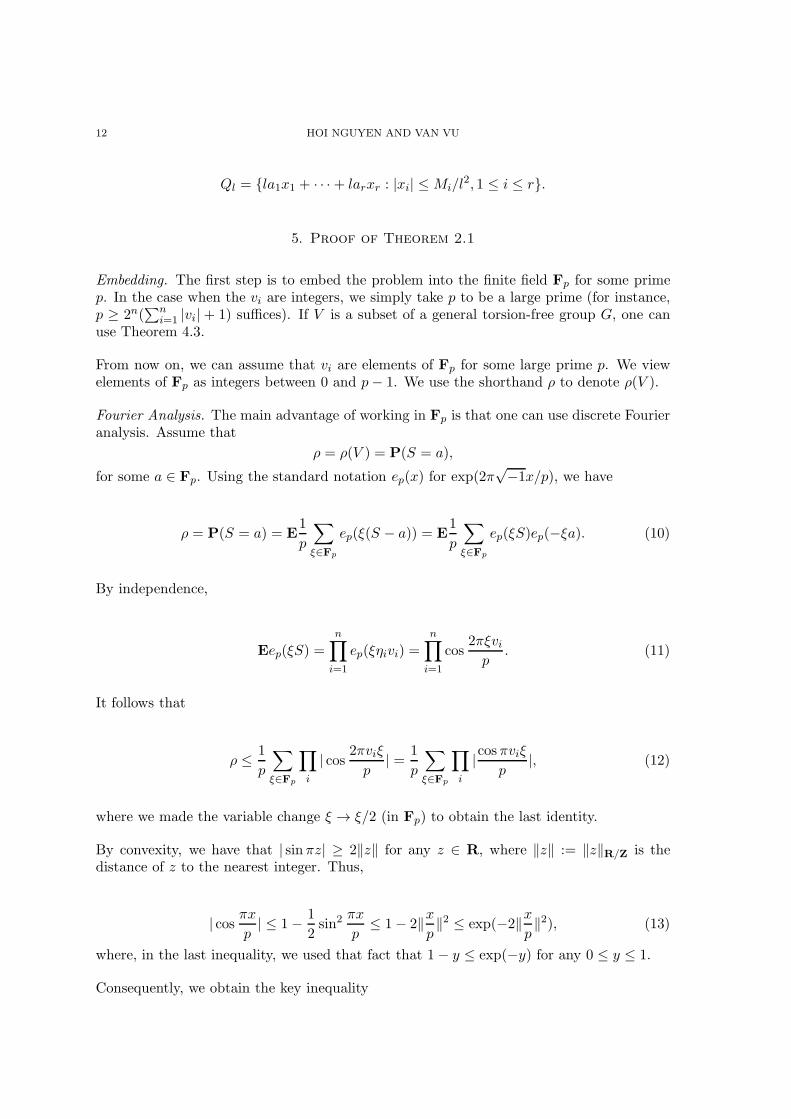
12 HOI NGUYEN AND VAN VU
Ql = la1x1 + · · ·+ larxr : |xi| ≤ Mi/l2, 1 ≤ i ≤ r.
5. Proof of Theorem 2.1
Embedding. The first step is to embed the problem into the finite field Fp for some primep. In the case when the vi are integers, we simply take p to be a large prime (for instance,p ≥ 2n(
∑ni=1 |vi| + 1) suffices). If V is a subset of a general torsion-free group G, one can
use Theorem 4.3.
From now on, we can assume that vi are elements of Fp for some large prime p. We viewelements of Fp as integers between 0 and p− 1. We use the shorthand ρ to denote ρ(V ).
Fourier Analysis. The main advantage of working in Fp is that one can use discrete Fourieranalysis. Assume that
ρ = ρ(V ) = P(S = a),
for some a ∈ Fp. Using the standard notation ep(x) for exp(2π√−1x/p), we have
ρ = P(S = a) = E1
p
∑
ξ∈Fp
ep(ξ(S − a)) = E1
p
∑
ξ∈Fp
ep(ξS)ep(−ξa). (10)
By independence,
Eep(ξS) =
n∏
i=1
ep(ξηivi) =
n∏
i=1
cos2πξvip
. (11)
It follows that
ρ ≤ 1
p
∑
ξ∈Fp
∏
i
| cos 2πviξp
| = 1
p
∑
ξ∈Fp
∏
i
|cos πviξp
|, (12)
where we made the variable change ξ → ξ/2 (in Fp) to obtain the last identity.
By convexity, we have that | sinπz| ≥ 2‖z‖ for any z ∈ R, where ‖z‖ := ‖z‖R/Z is thedistance of z to the nearest integer. Thus,
| cos πxp| ≤ 1− 1
2sin2
πx
p≤ 1− 2‖x
p‖2 ≤ exp(−2‖x
p‖2), (13)
where, in the last inequality, we used that fact that 1− y ≤ exp(−y) for any 0 ≤ y ≤ 1.
Consequently, we obtain the key inequality
INVERSE LITTLEWOOD-OFFORD PROBLEM 13
ρ ≤ 1
p
∑
ξ∈Fp
∏
i
| cos πviξp
| ≤ 1
p
∑
ξ∈Fp
exp(−2
n∑
i=1
‖viξp
‖2). (14)
Large level sets. Now, we consider the level sets Sm := ξ|∑n
i=1 ‖viξ/p‖2 ≤ m. We have
n−C ≤ ρ ≤ 1
p
∑
ξ∈Fp
exp(−2n∑
i=1
‖viξp
‖2) ≤ 1
p+
1
p
∑
m≥1
exp(−2(m− 1))|Sm|.
Because∑
m≥1 exp(−m) < 1, there must be a large level set Sm such that
|Sm| exp(−m+ 2) ≥ ρp. (15)
In fact, because ρ ≥ n−C , we can assume that m = O(log n).
Double counting and the triangle inequality. By double -counting, we have
n∑
i=1
∑
ξ∈Sm
‖viξp
‖2 =∑
ξ∈Sm
n∑
i=1
‖viξp‖2 ≤ m|Sm|.
So, for most vi
∑
ξ∈Sm
‖viξp
‖2 ≤ C0m
n|Sm| (16)
for some large constant C0.
Set C0 = ε−1. By averaging, the set of vi satisfying (16) has a size of at least (1− ε)n. Wecall this set V ′. The set V \V ′ has a size of at most εn, and this is the exceptional set thatappears in Theorem 2.1. In the rest of the proof, we are going to show that V ′ is a densesubset of a proper GAP.
Because ‖ · ‖ is a norm, by the triangle inequality, we have, for any a ∈ kV ′,
∑
ξ∈Sm
‖aξp‖2 ≤ k2
C0m
n|Sm|. (17)
More generally, for any l ≤ k and a ∈ lV ′,
∑
ξ∈Sm
‖aξp‖2 ≤ k2
C0m
n|Sm|. (18)
14 HOI NGUYEN AND VAN VU
Dual sets. Define S∗m := a|∑ξ∈Sm
‖aξp ‖2 ≤ 1
200 |Sm| (the constant 200 is ad hoc, and any
sufficiently large constant would be sufficient). S∗m can be viewed as some sort of a dual set
of Sm. In fact, one can show, as far as cardinality is concerned, it does behave like a dual
|S∗m| ≤ 8p
|Sm| . (19)
To see this, define Ta :=∑
ξ∈Smcos 2πaξ
p . Using the fact that cos 2πz ≥ 1− 100‖z‖2 for any
z ∈ R, we have, for any a ∈ S∗m
Ta ≥∑
ξ∈Sm
(1− 100‖aξp‖2) ≥ 1
2|Sm|.
However, using the basic identity∑
a∈Fpcos 2πax
p = pIx=0, we have
∑
a∈Fp
T 2a ≤ 2p|Sm|.
(19) follows from the last two estimates and averaging.
Set k := c1√
nm , for a properly chosen constant c1 = c1(C0). By (18), we have ∪k
l=1lV′ ⊂ S∗
m.
Set V′′
= V ′ ∪ 0; we have kV′′ ⊂ S∗
m ∪ 0. This results in the critical bound
|kV ′′ | = O(p
|Sm|) = O(ρ−1 exp(−m+ 2)). (20)
The long range inverse theorem. The role of Fp is no longer important, so we can viewthe vi as integers. The inequality (20) is exactly the assumption of the long range inversetheorem.
With this theorem in hand, we are ready to conclude the proof. A slight technical problem isthat V
′′
is not a set but a multiset. Thus, we apply Theorem 3.2 with X as the set of distinct
elements of V′′
(note that kX = kV ′′ if k ≥ 2). Furthermore, k = Ω(√
nm) = Ω(
√
nlogn),
ρ−1 ≤ nC is bounded from above by k2C+1.
It follows from Theorem 3.2 that X is a subset of a proper symmetric GAP Q of rankr = OC,ǫ(1) and cardinality
OC,ǫ(k−r|kX|) = OC,ǫ(k
−r|kV ′′ |) = OC,ǫ
(
ρ−1 exp(−m)(
√
n
m)−r
)
= OC,ǫ(ρ−1n−r),
concluding the proof.
INVERSE LITTLEWOOD-OFFORD PROBLEM 15
Remark 5.1. To prove Theorem 2.5, in the section describing double counting and the tri-angle inequality, we define V ′ to be the collection of all vi ∈ V satisfying
∑
ξ∈Sm
‖viξp
‖2 ≤ m
n′ |Sm|.
Next, with k = c1
√
n′
m for some sufficiently small c1, we obtain a bound similar to (20),
where |kV ′′| = O(ρ−1 exp(−m+ 2)). We then conclude Theorem 2.5 by applying the longrange inverse theorem.
6. Proof of Theorem 2.9
This proof will essentially follow the same steps as in the discrete case, with some additionalsimple arguments.
Given a real number w and a variable z, we define the z-norm of w by
‖w‖z := (E‖w(z1 − z2)‖2)1/2,
where z1, z2 are two iid copies of z.
Fourier analysis. Our first step is to obtain the following analogue of (14), using the Fouriertransform.
Lemma 6.1 (bounds for small ball probability).
ρr,z(V ) ≤ exp(πr2)
∫
Rd
exp(−n∑
i=1
‖〈vi, ξ〉‖2z/2− π‖ξ‖22)dξ.
This lemma is basically from [21]; the proof is presented in Appendix C, for the reader’sconvenience.
Next, consider the multiset Vβ := β−1 · V = β−1v1, . . . , β−1vn. It is clear that
ρβ,z(V ) = ρ1,z(Vβ).
We now work with Vβ. Thus ρ1,z(Vβ) ≥ n−O(1) and∑
v∈Vβ‖v‖2 = β−2.
For concision, we write ρ for ρ1,z(Vβ). Set M := 2A log n, where A is sufficiently large.
From Lemma 6.1 and the fact that ρ ≥ n−O(1), we easily obtain
∫
‖ξ‖2≤Mexp(−1
2
∑
v∈Vβ
‖〈v, ξ〉‖2z − π‖ξ‖22)dξ ≥ ρ
2. (21)
16 HOI NGUYEN AND VAN VU
Large level sets. For each integer 0 ≤ m ≤ M , we define the level set
Sm :=
ξ ∈ Rd :∑
v∈Vβ
‖〈v, ξ〉‖2z + ‖ξ‖22 ≤ m
.
Then, it follows from (21) that∑
m≤M µ(Sm) exp(−m2 + 1) ≥ ρ, where µ(.) denotes the
Lebesgue measure of a measurable set. Hence, there exists m ≤ M such that µ(Sm) ≥ρ exp(m4 − 2).
Next, because Sm ⊂ B(0,√m), by the pigeon-hole principle there exists a ball B(x, 12 ) ⊂
B(0,√m) such that
µ(B(x,1
2) ∩ Sm) ≥ cdµ(Sm)m−d/2 ≥ cdρ exp(
m
4− 2)m−d/2.
Consider ξ1, ξ2 ∈ B(x, 1/2) ∩ Sm. By the Cauchy-Schwarz inequality (note that ‖.‖z is anorm), we have
∑
v∈Vβ
‖〈v, (ξ1 − ξ2)〉‖2z ≤ 4m.
Because ξ1 − ξ2 ∈ B(0, 1) and µ(B(x, 12)∩Sm −B(x, 12)∩Sm) ≥ µ(B(x, 12 )∩ Sm), if we put
T := ξ ∈ B(0, 1),
n∑
i=1
‖〈ξ, vi〉‖2z ≤ 4m,
then
µ(T ) ≥ cdρ exp(m
4− 2)m−d/2.
Discretization. Choose N to be a sufficiently large prime (depending on the set T ). Definethe discrete box
B0 := (k1/N, . . . , kd/N) : ki ∈ Z,−N ≤ ki ≤ N .
We consider all shifted boxes x + B0, where x ∈ [0, 1/N ]d. By the pigeon-hole principle,there exists x0 such that the size of the discrete set (x0+B0)∩T is at least the expectation|(x0 +B0) ∩ T | ≥ Ndµ(T ) (to see this, we first consider the case when T is a box).
Let us fix some ξ0 ∈ (x0 +B0) ∩ T . Then, for any ξ ∈ (x0 +B0) ∩ T , we have
INVERSE LITTLEWOOD-OFFORD PROBLEM 17
∑
v∈Vβ
‖〈v, ξ0 − ξ〉‖2z ≤ 2
∑
v∈Vβ
‖〈v, ξ〉‖2z +∑
v∈Vβ
‖〈v, ξ0〉‖2z
≤ 16m.
Note that ξ0 − ξ ∈ B1 := B0 − B0 = (k1/N, . . . , kd/N) : ki ∈ Z,−2N ≤ ki ≤ 2N. Thus,
there exists a subset S of size at least cdNdρ exp(m4 −2)m−d/2 of B1 such that the following
holds for any s ∈ S:
∑
v∈Vβ
‖〈v, s〉‖2z ≤ 16m.
Double counting. We let y = z1 − z2, where z1, z2 are iid copies of z. By the definition ofS, we have
∑
s∈S
∑
v∈Vβ
‖〈v, s〉‖2z ≤ 16m|S|
Ey
∑
s∈S
∑
v∈Vβ
‖y〈v, s〉‖2R/Z ≤ 16m|S|.
It is then implied that there exists 1 ≤ |y0| ≤ Cz such that
∑
s∈S
∑
v∈Vβ
‖y0〈v, s〉‖2R/Z ≤ 16m|S|P(1 ≤ |y| ≤ Cz)−1.
However, by property (7), we have P(1 ≤ |y| ≤ Cz) ≥ 1/2. Thus,
∑
s∈S
∑
v∈Vβ
‖y0〈v, s〉‖2R/Z ≤ 32m|S|.
Let n′ be any number between nǫ and n. We say that v ∈ Vβ is bad if
∑
s∈S‖y0〈v, s〉‖2R/Z ≥ 32m|S|
n′ .
Then, the number of bad vectors is at most n′. Let V ′β be the set of remaining vectors.
Thus, V ′β contains at least n− n′ elements. In the remainder of the proof, we show that V ′
β
is close to a GAP, as claimed in the theorem.
Dual sets. Consider an arbitrary v ∈ V ′β. We have
∑
s∈S ‖y0〈s, v〉‖2R/Z ≤ 32m|S|/n′.
18 HOI NGUYEN AND VAN VU
Set k :=√
n′
64π2m , and let V ′′β := k(V ′
β ∪ 0). By the Cauchy-Schwarz inequality (see (18)),
for any a ∈ V ′′β , we have
∑
s∈S2π2‖〈s, y0a〉‖2R/Z ≤ |S|
2,
which implies
∑
s∈Scos(2π〈s, y0a〉) ≥
|S|2.
Observe that, for any x ∈ C(0, 1256d ) (the ball of radius 1/256d in the ‖.‖∞ norm) and any
s ∈ S ⊂ C(0, 2), we always have cos(2π〈s, x〉) ≥ 1/2 and sin(2π〈s, x〉) ≤ 1/12. Thus, forany x ∈ C(0, 1
256d ),
∑
s∈Scos (2π〈s, (y0a+ x)〉) ≥ |S|
4− |S|
12=
|S|6.
However,
∫
x∈[0,N ]d
(
∑
s∈Scos(2π〈s, x〉)
)2
dx ≤∑
s1,s2∈S
∫
x∈[0,N ]dexp
(
2π√−1〈s1 − s2, x〉
)
dx
≪d |S|Nd.
Hence, we deduce the following:
µx∈[0,N ]d
(
(∑
s∈Scos(2π〈s, x〉))2 ≥ (
|S|6)2
)
≪d|S|Nd
(|S|/6)2 ≪dNd
|S| .
Now, using the facts that S is large, |S| ≫d Ndρ exp(m4 − 2)m−d/2 and N was chosen to be
large enough for y0V′′β + C(0, 1
256d ) ⊂ [0, N ]d, we have
µ(y0V′′β +C(0,
1
256d)) ≪d ρ
−1 exp(−m
4+ 2)md/2.
Thus, we obtain the following analogue of (20):
INVERSE LITTLEWOOD-OFFORD PROBLEM 19
µ
(
k(V ′β ∪ 0) + C(0,
1
256dy0)
)
≪d ρ−1y−d
0 exp(−m
4+ 2)md/2. (22)
The long range inverse theorem. Our analysis again relies on the long range inverse theorem.Let D := 1024dy0. We approximate each vector v′ of V ′
β by its closest vector in ( Z
Dk )d,
‖v′ − a
Dk‖2 ≤
√d
Dk, with a ∈ Zd.
Let Aβ be the collection of all such a. Because∑
v′∈V ′
β‖v′‖22 = O(β−2), we have
∑
a∈Aβ
‖a‖22 = Od,Cz(k2β−2). (23)
It follows from (22) that
|k(Aβ + C0(0, 1))| = Od,Cz
(
ρ−1(Dk)dy−d0 exp(−m
4+ 2)md/2
)
= Od,Cz
(
ρ−1kd exp(−m
4+ 2)md/2
)
,
where C0(0, r) is the discrete cube (z1, . . . , zd) ∈ Zd : |zi| ≤ r.
Now, we apply Theorem 3.2 to the set Aβ+C0(0, 1) (note that 0 ∈ Aβ). That lemma implies
there exists a proper GAP P = ∑r
i=1 xigi : |xi| ≤ Ni ⊂ Zd containing Aβ +C0(0, 1) witha small rank r = O(1) and small size
|P | = Od,Cz
(
(ρ−1kd exp(−m
4+ 2)md/2k−r
)
= Od,Cz (ρ−1n′(−r+d)/2
).
Moreover, we learned from the proof of Theorem 3.2 and Lemma 4.4 that kQ can becontained in a set ck(Aβ + C0(0, 1)) for some c = O(1). Using (23), we conclude that allgenerators gi of Q are bounded,
‖gi‖2 = Od,Cz (kβ−1).
Next, because C0(0, 1) ⊂ Q, the rank r of P is at least d. It is a routine calculation to see
that Q := βDk · P satisfies all of the required properties in Theorem 2.9.
20 HOI NGUYEN AND VAN VU
Appendix A. Proof of the long range inverse theorem
The key lemma to prove our long range inverse theorem is an earlier result by Tao and thesecond author ([19, Theorem 1.21]), given below.
Lemma A.1. Let ǫ > 0, γ > 0 be constants. Assume that X is a subset of integers suchthat |kX| ≤ kγ |X| for some number k ≥ 2. Then, kX is contained in a symmetric 2-properGAP Q with rank r = Oγ,ǫ(1) and cardinality Oγ,ǫ(|kX|).
Next, if kX ⊂ kQ, where Q is a GAP, then it is natural to suspect that X ⊂ Q, but this isnot always true. However, the conclusion holds if kQ is 2-proper and 0 ∈ X.
Lemma A.2. (Dividing sumsets relations) Assume that 0 ∈ X and that P = ∑r
i=1 xiai :|xi| ≤ Ni is a symmetric 2-proper GAP that contains kX. Then X ⊂ ∑r
i=1 xiai : |xi| ≤2Ni/k.
A good way to keep this lemma in mind is the following. Consider the relation X ⊂ P . It istrivial that this relation can always be multiplied, namely, for all integers k ≥ 1, kX ⊂ kP .The above lemma asserts that, under certain assumptions, the relation kX ⊂ kP can bedivided, giving X ∈ P .
Proof. (of Lemma A.2) Without a loss of generality, we can assume that k = 2l. It issufficient to show that 2l−1X ⊂ ∑r
i=1 xiai : |xi| ≤ Ni/2. Because 0 ∈ X, 2l−1X ⊂ 2lX ⊂P , any element x of 2l−1X can be written as x =
∑ri=1 xiai, with |xi| ≤ Ni. Now, because
2x ∈ P ⊂ 2P and 2P is proper (as P is 2-proper), we must have 0 ≤ |2xi| ≤ Ni.
It is clear that Theorem 3.2 follows from Lemma A.1 and Lemma A.2.
Appendix B. Remarks on Theorem 2.9
The purpose of this section is to give an example showing that the bound in Theorem 2.9cannot be improved and to provide a proof for Corollary 2.10.
First, consider the set U := [−2n,−n] ∪ [n, 2n]. Sample n points v1, . . . , vn from U inde-pendently with respect to the (continuous) uniform distribution, and let A be the set ofsampled points. Let ξ be the Gaussian random variable N(0, 1), and consider the sum
S := v1ξ1 + · · ·+ vnξn,
where ξi are iid copies of ξ.
S has a Gaussian distribution with a mean 0 and variance Θ(n3), with a probability of one.
Thus, for some interval I of length 1, P(S ∈ I) ≥ Cn−3/2, for some constant C.
Set n′ = δn, for some small positive constant δ. Theorem 2.9 states that (most of) A is
O( logn√n)-close to a GAP of rank r and volume O(n2− r
2 ). We show that one cannot replace
INVERSE LITTLEWOOD-OFFORD PROBLEM 21
this bound by O(n2− r2−ǫ) for any ǫ. There are only three possible values for r: r = 1, 2, 3.
Our claim follows from the following simple lemma, whose proof remains as an exercise.
Lemma B.1. Let C, δ, ǫ be positive constants and n → ∞. The following hold with aprobability of 1− o(1) (with respect to the random choice of A).
• A does not contain any subset of cardinality (1− δ)n that is C logn√n
-close to a GAP
of rank 1 and volume of at most Cn3/2−ǫ.
• A does not contain any subset of cardinality (1− δ)n that is C logn√n
-close to a GAP
of rank 2 and volume of at most Cn1−ǫ.
• A does not contain any subset of cardinality (1− δ)n that is C logn√n
-close to a GAP
of rank 3 and volume of at most Cn1/2−ǫ.
The construction above can also be generalized to higher dimensions, but we do not attemptto do so here.
For the remainder of this section, we prove Corollary 2.10.
We consider the following two cases.
Case 1: r ≥ d + 1. Consider the GAP P at the end of the proof of Theorem 2.9. Recall
that |P | = Od,Cz(ρ−1n′(d−r)/2) = Od,Cz(ρ
−1/√n′). Let
Q :=β
Dk· P.
It is clear that Q satisfies all of the conditions of Corollary 2.10. (Note that, in this case,
we obtain a stronger approximation; almost all elements of V are O(β logn′
√n′
)-close to Q.)
Case 2: r = d. Because the unit vectors ej = (0, . . . , 1, . . . , 0) belong to P = ∑di=1 xigi :
|xi| ≤ Ni ⊂ Zd, the set of generators gi, i = 1, . . . , d forms a base with the unit determinantof Rd. In P , consider the set of lattice points with all coordinates divisible by k. We observethat (for instance, by [23, Theorem 3.36]) this set can be contained in a GAP P ′ of rank
d and cardinality max(
O( 1kr |P |, 1
)
= max(
O(ρ−1/n′r/2), 1)
. (Here, we use the bound
|P | = O(ρ−1 exp(−m4 )m
d/2).) Next, define
Q :=β
Dk· P ′.
It is easy to verify that Q satisfies all of the conditions of Corollary 2.10. (Note that, inthis case, we obtain a stronger bound on the size of Q.)
22 HOI NGUYEN AND VAN VU
Appendix C. Proof of Lemma 6.1
We have
P(n∑
i=1
zivi ∈ B(x, r)) = P(‖n∑
i=1
zivi − x‖22 ≤ r2)
= P
(
exp(−π‖n∑
i=1
zivi − x‖22) ≥ exp(−πr2)
)
≤ exp(πr2)E exp(−π‖n∑
i=1
zivi − x‖22).
Note that
exp(−π‖x‖22) =∫
Rd
e(〈x, ξ〉) exp(−π‖ξ‖22)dξ.
We thus have
P(
n∑
i=1
zivi ∈ B(x, r)) ≤ exp(πr2)
∫
Rd
Ee(〈n∑
i=1
zivi, ξ〉)e(−〈x, ξ〉) exp(−π‖ξ‖22)dξ.
Using
|Ee(〈n∑
i=1
zivi, ξ〉)| =n∏
i=1
|Ee(zi〈vi, ξ〉)|,
and
|Ee(zi〈vi, ξ〉)| ≤ |Ee(zi〈vi, ξ〉)|2/2 + 1/2 ≤ exp(−‖〈vi, ξ〉‖2z/2),
we obtain
ρr,z(V ) ≤ exp(πr2)
∫
Rd
exp(−n∑
i=1
‖〈vi, ξ〉‖2z/2− π‖ξ‖22)dξ.
Acknowledgements. The authors would like to thank K. Costello and the referees forcarefully reading this manuscript and providing very helpful remarks.
INVERSE LITTLEWOOD-OFFORD PROBLEM 23
References
[1] P. Erdos, On a lemma of Littlewood and Offord, Bull. Amer. Math. Soc. 51 (1945), 898-902.[2] P. Erdos and L. Moser, Elementary Problems and Solutions: Solutions: E736. Amer. Math. Monthly,
54 (1947), no. 4, 229-230.[3] J. Griggs, Database Security and the Distribution of Subset Sums in R
m, Graph Theory and Combina-torial Biology, Balatonlelle 1996 , Bolyai Math. Studs. 7 (1999), 223–252.
[4] G. Halasz, Estimates for the concentration function of combinatorial number theory and probability,Period. Math. Hungar. 8 (1977), no. 3-4, 197-211.
[5] G. Katona, On a conjecture of Erdos and a stronger form of Sperner’s theorem. Studia Sci. Math.Hungar 1 (1966), 59–63.
[6] D. Kleitman, On a lemma of Littlewood and Offord on the distributions of linear combinations of vectors,Advances in Math. 5 (1970), 155-157.
[7] J. E. Littlewood and A. C. Offord, On the number of real roots of a random algebraic equation. III. Rec.Math. Mat. Sbornik N.S. 12 , (1943). 277–286.
[8] H. Nguyen, A new approach to an old problem of Erdos and Moser, submitted.[9] R. A. Proctor, Solution of two difficult combinatorial problems with linear algebra. Amer. Math. Monthly
89 (1982), no. 10, 721-734.[10] M. Rudelson and R. Vershynin, The Littlewood-Offord problem and the condition number of random
matrices, Advances in Mathematics 218 (2008), no 2, 600-633.[11] A. Sarkozy, Finite addition theorems I, J. Num. Thy. 32 (1989), 114–130.
[12] A. Sarkozy and E. Szemeredi, Uber ein Problem von Erdos und Moser, Acta Arithmetica, 11 (1965)205-208.
[13] R. Stanley, Weyl groups, the hard Lefschetz theorem, and the Sperner property, SIAM J. AlgebraicDiscrete Methods 1 (1980), no. 2, 168–184.
[14] E. Szemeredi and V. Vu, Long arithmetic progressions in sumsets: thresholds and bounds, J. Amer.Math. Soc. 19 (2006), 119–169.
[15] T. Tao, Freiman’s theorem in solvable groups, http://arxiv.org/abs/0906.3535[16] T. Tao and V. Vu, A sharp inverse Littlewood-Offord theorem, to appear in Random Structures and
Algorithms.[17] T. Tao and V. Vu, From the Littlewood-Offord problem to the circular law: universality of the spectral
distribution of random matrices, Bull. Amer. Math. Soc. (N.S.) 46 (2009), no. 3, 377–396.[18] T. Tao and V. Vu, Inverse Littlewood-Offord theorems and the condition number of random matrices,
Annals of Mathematics (2) 169 (2009), no 2, 595-632.[19] T. Tao and V. Vu, John-type theorems for generalized arithmetic progressions and iterated sumsets,
Adv. Math. 219 (2008), no. 2, 428–449.[20] T. Tao and V. Vu, On the singularity probability of random Bernoulli matrices, Journal of the A. M. S
20 (2007), 603-673.[21] T. Tao and V. Vu, Random matrices: The Circular Law, Communication in Contemporary Mathematics
10 (2008), 261-307.[22] T. Tao and V. Vu, Smooth analysis of the condition number and the least singular value, (to appear in
Mathematics of Computation).[23] T. Tao and V. Vu, Additive Combinatorics, Cambridge Univ. Press, 2006.
Department of Mathematics, Rutgers University, Piscataway, NJ 08854
E-mail address: [email protected]
Department of Mathematics, Rutgers University, Piscataway, NJ 08854
E-mail address: [email protected]