Stat PapersDOI 10.1007/s00362-009-0271-3

REGULAR ARTICLE

The generalized inverse Weibull distribution

Felipe R. S. de Gusmão · Edwin M. M. Ortega ·Gauss M. Cordeiro

Received: 2 February 2009 / Revised: 21 July 2005© Springer-Verlag 2009

Abstract The inverse Weibull distribution has the ability to model failure rateswhich are quite common in reliability and biological studies. A three-parameter gen-eralized inverse Weibull distribution with decreasing and unimodal failure rate isintroduced and studied. We provide a comprehensive treatment of the mathematicalproperties of the new distribution including expressions for the moment generatingfunction and the r th generalized moment. The mixture model of two generalizedinverse Weibull distributions is investigated. The identifiability property of the mix-ture model is demonstrated. For the first time, we propose a location-scale regressionmodel based on the log-generalized inverse Weibull distribution for modeling lifetimedata. In addition, we develop some diagnostic tools for sensitivity analysis. Two appli-cations of real data are given to illustrate the potentiality of the proposed regressionmodel.

Keywords Censored data · Data analysis · Inverse Weibull distribution · Maximumlikelihood estimation · Moment · Weibull regression model

F. R. S. de Gusmão · G. M. CordeiroDEINFO, Universidade Federal Rural de Pernambuco, Recife, Brazil

F. R. S. de Gusmãoe-mail: felipe556@gmail.com

G. M. Cordeiroe-mail: gausscordeiro@uol.com.br

E. M. M. Ortega (B)Departamento de Ciências Exatas, ESALQ, Universidade de São Paulo, Av. Pádua Dias 11,Caixa Postal 9, Piracicaba, SP 13418-900, Brazile-mail: edwin@esalq.usp.br

123

F. R. S. de Gusmão et al.

1 Introduction

The inverse Weibull (IW) distribution has received some attention in the literature.Keller and Kamath (1982) study the shapes of the density and failure rate functionsfor the basic inverse model. The random variable Y has an inverse Weibull distributionif its cumulative distribution function (cdf) takes the form

G(t) = exp

[−(α

t

)β]

, t > 0, (1)

where α > 0 and β > 0. The corresponding probability density function (pdf) is

g(t) = βαβ t−(β+1) exp

[−(α

t

)β]

. (2)

The IW distribution is also a limiting distribution of the largest order statistics. Drapella(1993) and Mudholkar and Kollia (1994) suggested the names complementary Weibulland reciprocal Weibull for the distribution (2). The corresponding survival and hazardfunctions are

SG(t) = 1 − G(t) = 1 − exp

[−(α

t

)β]

and

hG(t) = βαβ t−(β+1) exp

[−(α

t

)β]{

1 − exp

[−(α

t

)β]}−1

,

respectively. The kth moment about zero of (2) is

E(T k) = αk�(1 − kβ−1),

where �(·) is the gamma function.The rest of the paper is organized as follows. In Sect. 2, we define the general-

ized inverse Weibull (GIW) distribution. Section 3 provides a general formula for itsmoments. General expansions for the moments of order statistics of the new distri-bution are given in Sect. 4. We discuss in Sect. 5 maximum likelihood estimationwith censored data. Section 6 provides some properties of a mixture of two GIWdistributions. Sections 7 and 8 discuss the log-generalized inverse Weibull distribu-tion and the corresponding regression model, respectively. Some diagnostic measuresfor the log-generalized inverse Weibull model are proposed in Sect. 9. Section 10defines two type of residuals. Section 11 illustrates two applications to real datasets including the model fitting and influence analysis. Section 12 ends with someconclusions.

123

The generalized inverse Weibull distribution

2 The generalized inverse Weibull distribution

Let G(t) be the cdf of the inverse Weibull distribution discussed by Drapella (1993),Mudholkar and Kollia (1994) and Jiang et al. (1999), among others. The cdf of theGIW distribution can be defined by elevating G(t) to the power of γ > 0, say F(t) =G(t)γ = exp

[−γ(

αt

)β]. Hence, the GIW density function with three parameters

α > 0, β > 0 and γ > 0 is given by

f (t) = γβαβ t−(β+1) exp

[−γ(α

t

)β]

, t > 0. (3)

We can easily prove that (3) is a density function by substituting u = −γαβ t−β . Theinverse Weibull distribution is a special case of (3) when γ = 1. If T is a randomvariable with density (3), we write T ∼ GIW(α, β, γ ). The corresponding survivaland hazard functions are

S(t) = 1 − F(t) = 1 − exp

[−γ(α

t

)β]

and

h(t) = γβαβ t−(β+1) exp

[−γ(α

t

)β]{

1 − exp

[−γ(α

t

)β]}−1

,

respectively.We can simulate the GIW distribution using the nonlinear equation

t = α

[− log(u)

γ

]−1/β

, (4)

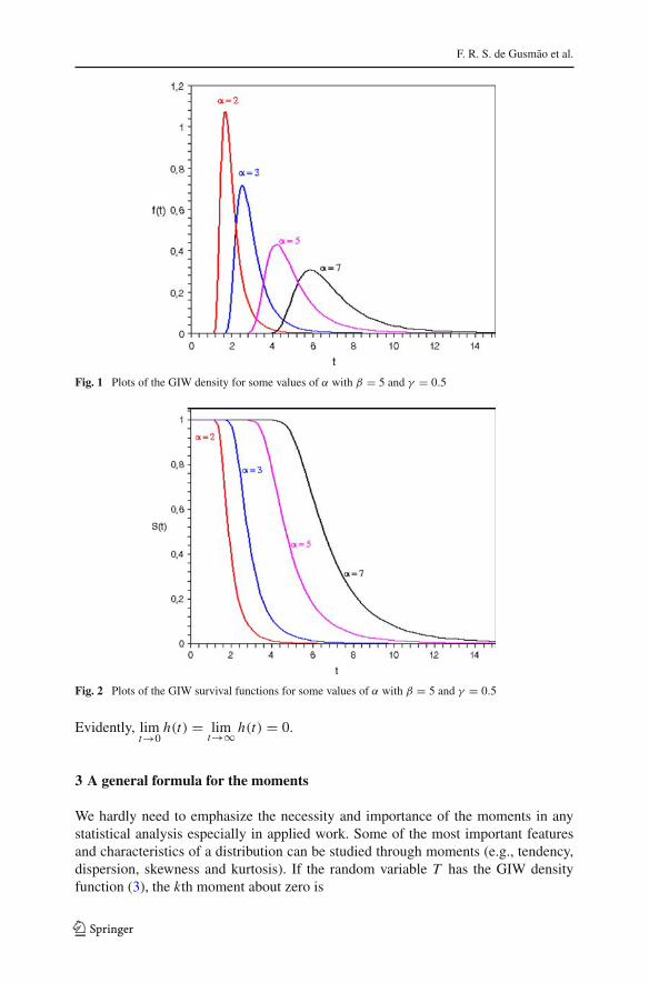
where u has the uniform U (0, 1) distribution. Plots of the GIW density and survivalfunction for selected parameter values are given in Figs. 1 and 2, respectively.

2.1 Characterizing the failure rate function

The first derivative h′(t) = dh(t)/dt to study the hazard function shape is given by

h′(t) = h(t)t−(β+1)

{γβαβ

{1 − exp

[−γ(α

t

)β]}−1

− (β + 1)tβ}

.

We can easily show that h(t) is unimodal with a maximum value at t∗, where t∗satisfies the nonlinear equation

γ( α

t∗){

1 − exp

[−γ( α

t∗)β]}−1

= 1 + β−1.

123

F. R. S. de Gusmão et al.

Fig. 1 Plots of the GIW density for some values of α with β = 5 and γ = 0.5

Fig. 2 Plots of the GIW survival functions for some values of α with β = 5 and γ = 0.5

Evidently, limt→0

h(t) = limt→∞ h(t) = 0.

3 A general formula for the moments

We hardly need to emphasize the necessity and importance of the moments in anystatistical analysis especially in applied work. Some of the most important featuresand characteristics of a distribution can be studied through moments (e.g., tendency,dispersion, skewness and kurtosis). If the random variable T has the GIW densityfunction (3), the kth moment about zero is

123

The generalized inverse Weibull distribution

E(T k) = γkβ αk�(1 − kβ−1). (5)

The moment generating function M(z) of T for |z| < 1 is

M(z) = E(ezT ) =n∑

k=0

{zk

k! γkβ αk�

(1 − kβ−1

)}.

Hence, for |z| < 1, the cumulant generating function of T is

K (z) = log[M(z)] = log

{n∑

k=0

[zk

k! γkβ αk�

(1 − kβ−1

)]}. (6)

The first four cumulants obtained from (6) are

κ1 = γ1β α�1(β), κ2 = γ

2β α2{�2(β) − �1(β)2},

κ3 = γ3β α3{�3(β) − 3�2(β)�1(β) + 2�1(β)3}

and

κ4 = γ4β α4{�4(β) − 4�3(β)�1(β) − 3�1(β)2 + 12�2(β)�1(β)2 − 6�1(β)4},

where �k(β) = �(1 − kβ−1) for k = 1, . . . , 4. The skewness and kurtosis are then

ρ3 = κ3/κ32

2 and ρ4 = κ4/κ22 , respectively.

The Shannon entropy of a random variable T with density f (t) is a measure of theuncertainty defined by E{− log[ f (T )]}. The Shannon entropy for the GIW distributioncan be expressed as

E{− log[ f (T )]} = − log(αβγ ) + (β + 1){log(α) + β−1[log(γ ) + 0.577216]} + 1,

where 0.577216 is the approximate value for Euler’s constant.

4 Moments of order statistics

Order statistics make their appearance in many areas of statistical theory and practice.Let the random variable Tr :n be the r th order statistic (T1:n ≤ T2:n ≤ · · · ≤ Tn:n) in asample of size n from the GIW distribution, for r = 1, . . . , n. The pdf of Tr :n is givenby

fr :n(t) = Cr :n f (t)F(t)r−1 [1 − F(t)]n−r , t > 0,

where f (t) comes from (3), F(t) = exp[−γ(

αt

)β] and Cr :n = n!/[(r −1)!(n −r)!].

123

F. R. S. de Gusmão et al.

The kth moment about zero of the r th order statistic is

µ(k)r :n = E(T k

r :n) = Cr :n∞∫

0

f (t)F(t)r−1 [1 − F(t)]n−r dt.

After some algebra, we can obtain

µ(k)r :n = Cr :nαkγ k/β �[1 − (k/β)]

n−r∑i=0

(n − r

i

)(−1)i (r + i)

kβ−1

. (7)

An alternative formula for this moment (Barakat and Abdelkader 2004) is

E(T kr :n) = k

n∑j=n−i+1

(−1) j−n+i−1(

j − 1

n − i

)(n

j

)I j (k), (8)

where I j (k) denotes the integral

I j (k) =∞∫

0

tk−1[1 − F(t)] j dt. (9)

From Eqs. 8 and 9, we have

E(T kr :n)=k(γ αβ)

kβ �k(β)

n∑j=n−i+1

j∑l=0

(−1) j−n+i−1(

j − 1

n − i

)(n

j

)(−1)l

(j

l

)l

kβ−1

.

(10)

For γ = 1, we obtain the moments of order statistics of the IW distribution. Equations7 and 10 are the main results of this section.

5 Maximum likelihood estimation with censored data

Let Ti be a random variable distributed as (3) with the vector of parameters θ =(α, β, γ )T . The data encountered in survival analysis and reliability studies are oftencensored. A very simple random censoring mechanism that is often realistic is onein which each individual i is assumed to have a lifetime Ti and a censoring time Ci ,where Ti and Ci are independent random variables. Suppose that the data consist ofn independent observations ti = min(Ti , Ci ) for i = 1, . . . , n. The distribution of Ci

does not depend on any of the unknown parameters of Ti . Parametric inference forsuch model is usually based on likelihood methods and their asymptotic theory. Thecensored log-likelihood l(θ) for the model parameters reduces to

123

The generalized inverse Weibull distribution

l(θ) = r[log(γ ) + log(β) + β log(α)

]− (β + 1)∑i∈F

log(ti ) − γαβ∑i∈F

t−βi

+∑i∈C

log

{1 − exp

[−γ

(α

ti

)β]}

,

where r is the number of failures and F and C denote the sets of uncensored andcensored observations, respectively.

The score functions for the parameters α, β and γ are given by

Uα(θ) = rβ

α− γβαβ−1

∑i∈F

t−βi + γβαβ−1

∑i∈C

t−βi

(1 − ui

ui

),

Uβ(θ) = r

β+ r log(α) −

∑i∈F

log(ti ) − γαβ∑i∈F

t−βi log

(α

ti

)

+γαβ∑i∈C

t−βi log

(α

ti

)(1 − ui

ui

)and

Uγ (θ) = r

γ− αβ

∑i∈F

t−βi + αβ

∑i∈C

t−βi

(1 − ui

ui

),

where ui = 1 − exp

[−γ(

αti

)β]

is the i th transformed observation.

The MLE θ of θ is obtained by solving the nonlinear likelihood equations Uα(θ) =0, Uβ(θ) = 0 and Uγ (θ) = 0 using iterative numerical techniques such as theNewton–Raphson algorithm. We employ the programming matrix language Ox(Doornik 2007).

For interval estimation of (α, β, γ ) and hypothesis tests on these parameters, wederive the observed information matrix since the expected information matrix is verycomplicated and requires numerical integration. The 3×3 observed information matrixJ (θ) is

J (θ) = −⎛⎝Lαα Lαβ Lαγ

· Lββ Lβγ

· · Lγ γ

⎞⎠ ,

whose elements are given in Appendix 1. Under conditions that are fulfilled for param-eters in the interior of the parameter space but not on the boundary, the asymptoticdistribution of

√n(θ − θ) is N3(0, I (θ)−1),

where I (θ) is the expected information matrix. This asymptotic behavior is valid ifI (θ) is replaced by J (θ), i.e., the observed information matrix evaluated at θ . Themultivariate normal N3(0, J (θ)−1) distribution can be used to construct approximateconfidence regions for the parameters and for the hazard and survival functions. The

123

F. R. S. de Gusmão et al.

asymptotic normality is also useful for testing goodness of fit of the GIW distributionand for comparing this distribution with some of its special sub-models using one ofthe three well-known asymptotically equivalent test statistics—namely, the likelihoodratio (LR) statistic, Wald and Rao score statistics.

6 Mixture of two GIW distributions

Mixture distributions have been considered extensively by many authors. For an excel-lent survey of estimation techniques, discussion and applications, see Everitt and Hand(1981), Maclachlan and Krishnan (1997) and Maclachlan and Peel (2000). Recently,AL-Hussaini and Sultan (2001), Jiang et al. (2001) and Sultan et al. (2007) reviewedsome properties and estimation techniques of finite mixtures for some lifetime models.

The mixture of two generalized inverse Weibull (MGIW) distributions has densitygiven by

f (t; θ) =2∑

i=1

pi fi (t; θ i ),

where∑2

i=1 pi = 1, θ = (θT1 , θT

2 )T , θ1 = (α1, β1, γ1)T , θ2 = (α2, β2, γ2)

T andfi (t; θ i ) is the density function of the i th component given by

fi (t; θi ) = γiβiαβii t−(βi +1) exp

[−γi

(αi

t

)βi]

, t, αi , βi , γi > 0, i = 1, 2.

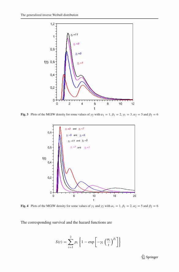
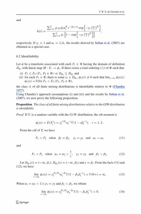
Different shapes of the MGIW density are shown in Figs. 3 and 4. The cdf of theMGIW distribution can be expressed as

F(t; θ) =2∑

i=1

pi Fi (t; θ i ),

where Fi (t; θi ) = exp[−γi

(αit

)βi]

is the cdf of the i th GIW distribution for i = 1, 2.

6.1 Properties

Here, we derive some properties of the MGIW distribution by extending the corre-sponding results for the GIW distribution. The kth moment of the random variable Tfollowing the MGIW distribution (5) is given by

E(T k) =2∑

i=1

piγ

kβi

i αki �(1 − kβ−1

i ).

123

The generalized inverse Weibull distribution

Fig. 3 Plots of the MGIW density for some values of γ2 with α1 = 1, β1 = 2, γ1 = 3, α2 = 5 and β2 = 6

Fig. 4 Plots of the MGIW density for some values of γ1 and γ2 with α1 = 1, β1 = 2, α2 = 5 and β2 = 6

The corresponding survival and the hazard functions are

S(t) =2∑

i=1

pi

{1 − exp

[−γi

(αi

t

)βi]}

123

F. R. S. de Gusmão et al.

and

h(t) =∑2

i=1 piγiβiαβii t−(βi +1) exp

[−γi

(αit

)βi]

∑2i=1 pi

{1 − exp

[−γi

(αit

)βi]} ,

respectively. If γi = 1 and αi = 1/δi , the results derived by Sultan et al. (2007) areobtained as a special case.

6.2 Identifiability

Let φ be a transform associated with each Fi ∈ having the domain of definitionDφi with linear map M : Fi → φi . If there exists a total ordering (�) of such that

(i) F1 � F2 (F1, F2 ∈ ) ⇒ Dφ1 ⊆ Dφ2 and(ii) for each F1 ∈ , there is some s1 ∈ Dφ1 , φ1(s) �= 0 such that lims→s1 φ2(s)/

φ1(s) = 0 for F1 < F2 (F1, F2 ∈ ),

the class � of all finite mixing distributions is identifiable relative to (Chandra1977).Using Chandra’s approach (assumptions (i) and (ii)) and the results by Sultan et al.(2007), we now prove the following proposition.

Proposition The class of all finite mixing distributions relative to the GIW distributionis identifiable.

Proof If Ti is a random variable with the G I W distribution, the sth moment is

φi (s) = E(T si ) = γ

s/βii α−s

i �(1 − sβ−1i ), i = 1, 2.

From the cdf of Ti we have

F1 < F2 when β1 = β2, γ1 = γ2 and α1 < α2 (11)

and

F1 < F2 when α1 = α2 >1

t, γ1 = γ2 and β1 < β2. (12)

Let Dφ1(s) = (−∞, β1), Dφ2(s) = (−∞, β2) and s = β1. From the facts (11) and(12), we have

lims→β1

φ1(s) = γβ1/β11 α

−β11 �(1 − β1β

−11 ) = �(0+) = ∞. (13)

When α1 = α2 > 1/t ,γ1 = γ2 and β1 < β2, we obtain

lims→β1

φ2(s) = γβ1/β21 α

−β11 �(1 − β1β

−12 ) > 0. (14)

123

The generalized inverse Weibull distribution

Finally, the results (13) and (14) lead to

lims→β1

φ2(s)

φ1(s)= 0,

and then the identifiability is proved. � It is a much more difficult problem to study the identifiability of a mixture of n ≥ 3

distributions. Lack of identifiability gives no guarantee of convergence to the truevalues of parameters and therefore usually gives rise to confusing results.

7 The log-generalized inverse Weibull distribution

Let T be a random variable having the GIW density function (3). The random variableY = log(T ) has a log-generalized inverse Weibull (LGIW) distribution whose densityfunction, parameterized in terms of σ = 1/β and µ = log(α), is given by

f (y; γ, σ, µ)= γ

σexp

{−(

y − µ

σ

)− γ exp

[−(

y − µ

σ

)]}, −∞ < y < ∞

(15)

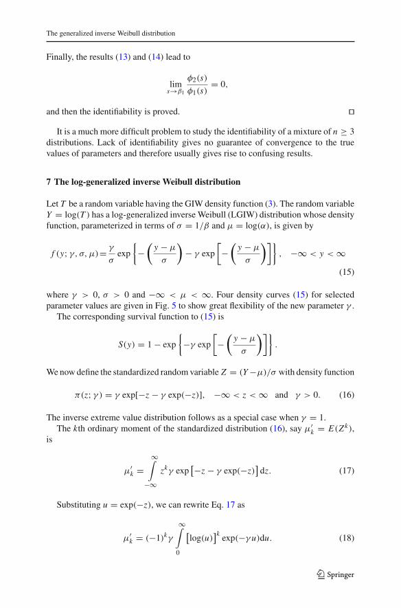
where γ > 0, σ > 0 and −∞ < µ < ∞. Four density curves (15) for selectedparameter values are given in Fig. 5 to show great flexibility of the new parameter γ .

The corresponding survival function to (15) is

S(y) = 1 − exp

{−γ exp

[−(

y − µ

σ

)]}.

We now define the standardized random variable Z = (Y −µ)/σ with density function

π(z; γ ) = γ exp[−z − γ exp(−z)], −∞ < z < ∞ and γ > 0. (16)

The inverse extreme value distribution follows as a special case when γ = 1.The kth ordinary moment of the standardized distribution (16), say µ′

k = E(Zk),is

µ′k =

∞∫−∞

zkγ exp[−z − γ exp(−z)

]dz. (17)

Substituting u = exp(−z), we can rewrite Eq. 17 as

µ′k = (−1)kγ

∞∫0

[log(u)

]k exp(−γ u)du. (18)

123

F. R. S. de Gusmão et al.

Fig. 5 Plots of the LGIW density for some parameter values

The integral in (18) follows from Prudnikov et al. (1986) and Nadarajah (2006) as

∞∫0

[log(u)]k exp(−γ u)du = ∂k[γ −a�(a)]∂ak

∣∣∣∣a=1

.

Inserting the last equation in (18), yields the kth moment of Z

µ′k = (−1)kγ

∂k[γ −a�(a)]∂ak

∣∣∣∣a=1

. (19)

The ordinary moments of Y can be obtained via binomial expansion and Eq. 19.

8 The log-generalized inverse Weibull regression model

In many practical applications, the lifetimes ti are affected by explanatory variablessuch as the cholesterol level, blood pressure and many others. Let xi = (xi1, . . . , xip)

T

be the explanatory variable vector associated with the i th response variable yi fori = 1, . . . , n. Consider a sample (y1, x1), . . . , (yn, xn) of n independent observations,where each random response is defined by yi = min{log(ti ), log(ci )}. We assumenon-informative censoring and that the observed lifetimes and censoring times areindependent.

For the first time, we construct a linear regression model for the response variableyi based on the LGIW density given by

yi = xTi β + σ zi , i = 1, . . . , n, (20)

123

The generalized inverse Weibull distribution

where the random error zi follows the distribution (16), β = (β1, . . . , βp)T , σ > 0

and γ > 0 are unknown scalar parameters and xi is the explanatory variable vectormodeling the location parameter µi = xT

i β. Hence, the location parameter vectorµ = (µ1, . . . , µn)T of the LGIW model has a linear structure µ = Xβ, whereX = (x1, . . . , xn)T is a known model matrix. The log-inverse Weibull (LIW) (or theinverse extreme value) regression model is defined by Eq. 20 with γ = 1.

Let F and C be the sets of individuals for which yi is the log-lifetime or log-censoring, respectively. The total log-likelihood function for the model parametersθ = (γ, σ,βT )T can be written from Eqs. 16 and 20 as

l(θ)=r[log(γ )−log(σ )

]−∑i∈F

(yi − xT

i β

σ

)−γ

∑i∈F

exp

[−(

yi − xTi β

σ

)]

+∑i∈C

log

[1 − exp

{−γ exp

[−(

yi − xTi β

σ

)]}], (21)

where r is the observed number of failures. The MLE θ of θ can be obtained by maxi-mizing the log-likelihood function (21). We use the matrix programming language Ox(MAXBFGS function) (see Doornik 2007) to compute this estimate. From the fittedmodel (20), the survival function for yi can be estimated by

S(yi ; γ , σ , βT) = 1 − exp

{−γ exp

[−(

yi − xTi β

σ

)]}.

Under general regularity conditions, the asymptotic distribution of√

n(θ − θ)

is multivariate normal Np+2(0, K (θ)−1), where K (θ) is the expected informationmatrix. The asymptotic covariance matrix K (θ)−1 of θ can be approximated by theinverse of the (p+2)×(p+2) observed information matrix J (θ) and then the asymp-totic inference for the parameter vector θ can be based on the normal approximationNp+2(0, J (θ)−1) for θ . The observed information matrix is

J (θ) = {−Lr,s} =⎛⎝−Lγ γ −Lγ σ −Lγβ j

· −Lσσ −Lσβ j

· · −Lβ j βs

⎞⎠ ,

whose elements are given in Appendix 2.The asymptotic multivariate normal Np+2(0, J (θ)−1) distribution can be used to

construct approximate confidence regions for some parameters in θ and for the hazardand survival functions. In fact, an 100(1 − α)% asymptotic confidence interval foreach parameter θr is given by

AC Ir =(

θr − zα/2

√−Lr,r

, θr + zα/2

√−Lr,r

),

123

F. R. S. de Gusmão et al.

where −Lr,rdenotes the r th diagonal element of the inverse of the estimated observed

information matrix J (θ)−1 and zα/2 is the quantile 1 − α/2 of the standard nor-mal distribution. The asymptotic normality is also useful for testing goodness offit of some sub-models and for comparing some special sub-models using the LRstatistic.

The interpretation of the estimated coefficients could be based on the ratio of mediantimes (see Hosmer and Lemeshow 1999) which holds for continuous or categoricalexplanatory variables. When the explanatory variable is binary (0 or 1), and consider-ing the ratio of median times with x = 1 in the numerator, if β is negative (positive),it implies that the individuals with x = 1 present reduced (increased) median survivaltime in [exp(β) × 100%] as compared to those individuals in the group with x = 0,assuming the other explanatory variables fixed.

We are also interested to investigate if the LIW model is a good model to fit thedata under investigation. Clearly, the LR statistic can be used to discriminate betweenthe LIW and LGIW models since they are nested models. The hypotheses to be testedin this case are H0 : γ = 1 versus H1 : γ �= 1 and the LR statistic reduces tow = 2{l (θ) − l (θ)}, where θ is the MLE of θ under H0. The null hypothesis isrejected if w > χ2

1−α(1), where χ21−α(1) is the quantile of the chi-square distribution

with one degree of freedom.

9 Sensitivity analysis

9.1 Global influence

A first tool to perform sensitivity analysis is by means of the global influence startingfrom case-deletion. Case-deletion is a common approach to study the effect of drop-ping the i th observation from the data set. The case-deletion model corresponding tomodel (20) is given by

yl = xTl β + σ zl , l = 1, . . . , n, and for l �= i. (22)

From now on, a quantity with subscript (i) refers to the original quantity with the i thobservation deleted. Let l(i)(θ) be the log-likelihood function for θ under model (22)

and θ (i) = (γ(i), σ(i), βT(i))

T be the MLE of θ obtained by maximizing l(i)(θ). To assess

the influence of the i th observation on the unrestricted estimate θ = (γ , σ , βT)T , the

basic idea is to compare the difference between θ (i) and θ . If deletion of an observa-tion seriously affect the estimates, more attention should be paid to that observation.Hence, if θ (i) is far from θ , then the ith case is regarded as an influential observation.A first measure of the global influence can be expressed as the standardized norm ofθ (i) − θ (so-called generalized Cook distance) given by

G Di (θ) = (θ (i) − θ)T J (θ)−1(θ (i) − θ).

Another alternative is to assess the values G Di (β) and G Di (γ, σ ) which reveal theimpact of the ith observation on the estimates of β and (γ, σ ), respectively. Another

123

The generalized inverse Weibull distribution

well-know measure of the difference between θ (i) and θ is the likelihood distance

L Di (θ) = 2{l (θ) − l (θ (i))}.

Further, we can also compute β j −β j (i)( j = 1, . . . , p) to obtain the difference betweenβ and β(i). Alternative global influence measures are possible. We can develop thebehavior of a test statistic, such as the Wald test for explanatory variable or censoringeffect, under a case deletion scheme.

9.2 Local influence

As a second tool for sensitivity analysis, we now describe the local influence methodfor the LGIW regression model with censored data. Local influence calculation can becarried out for the model (20). If likelihood displacement L D(ω) = 2{l (θ) − l (θω)}is used, where θω is the MLE under the perturbed model, the normal curvature forθ at the direction d, ‖ d ‖= 1, is given by Cd(θ) = 2|dT �T J (θ)−1�d| (see Cook1986). Here, � is a (p + 2)× n matrix depending on the perturbation scheme, whoseelements are given by � j i = ∂2l(θ |ω)/∂θ j∂ωi , i = 1, . . . , n and j = 1, . . . , p + 2evaluated at θ and ω0, and ω0 is the no perturbation vector. For the LGIW model, theelements of J (θ) are given in Appendix 2. We can calculate normal curvatures Cd(θ),Cd(γ ), Cd(σ ) and Cd(β) to perform various index plots, for instance, the index plotof dmax, the eigenvector corresponding to Cdmax , the largest eigenvalue of the matrixB = �T J (θ)−1� and the index plots of Cdi (θ), Cdi (γ ), Cdi (σ ) and Cdi (β), so-calledthe total local influence (see, for example, Lesaffre and Verbeke 1998), where di is ann×1 vector of zeros with one at the i th position. Hence, the curvature at direction di

has the form Ci = 2|�Ti J (θ)−1�i |, where �T

i is the i th row of �. It is usual to pointout those cases such that

Ci ≥ 2C, C = 1

n

n∑i=1

Ci .

9.3 Curvature calculations

Here, under three perturbation schemes, we calculate the matrix

� = (� j i )(p+2)×n =(

∂2l(θ |ω)

∂θiω j

)(p+2)×n

, j = 1, . . . , p + 2 and i = 1, . . . , n,

from the log-likelihood function (21). Let ω = (ω1, . . . , ωn)T be the vector of weights.

123

F. R. S. de Gusmão et al.

9.3.1 Case-weight perturbation

In this case, the log-likelihood function has the form

l(θ |ω) = [log(γ ) − log(σ )]∑

i∈F

ωi −∑i∈F

ωi zi − γ∑i∈F

ωi exp(−zi )

+∑i∈C

ωi log {1 − exp[−γ exp(−zi )]} ,

where zi = (yi − xTi β)/σ , 0 ≤ ωi ≤ 1 and ω = (1, . . . , 1)T . From now on, we take

� = (�1, . . . ,�p+2)T , zi = (yi − xT

i β)/σ and hi = exp[−γ exp(−zi )].The elements of the vector �1 have the form

�1i ={

γ −1 − exp(−zi ) if i ∈ Fhi exp(−zi )(1 − hi )

−1 if i ∈ C.

On the other hand, the elements of the vector �2 are

�2i ={

σ−1{−1 + zi [−1 + γ exp(−zi )]} if i ∈ Fγ σ−1 zi hi exp(−zi )(1 − hi )

−1 if i ∈ C.

The elements of the vector � j for j = 3, . . . , p + 2 can be expressed as

� j i ={

σ−1xi j[1 − γ exp(zi )

]if i ∈ F

γ σ−1xi j hi exp(−zi )(1 − hi )−1 if i ∈ C.

9.3.2 Response perturbation

We assume that each yi is perturbed as yiw = yi + ωi Sy , where Sy is a scale factorsuch as the standard deviation of Y and ωi ∈ �. The perturbed log-likelihood functionbecomes

l(θ |ω) = r[log(γ ) − log(σ )

]−∑i∈F

z∗i − γ

∑i∈F

exp(−z∗i )

+∑i∈C

log{1 − exp[−γ exp(−z∗

i )]},

where z∗i = [(yi + ωi Sy) − xT

i β]/σ . In addition, the elements of the vector �1 take

the form

�1i ={

σ−1Sy exp(zi ) if i ∈ F

σ−1Sy hi exp(−zi ){[γ exp(−zi ) − 1](

1 − hi

)+ hi exp(−zi )}(1 − hi )

−2 if i ∈ C.

123

The generalized inverse Weibull distribution

On the other hand, the elements of the vector �2 are

�2i =⎧⎨⎩

σ−2Sy[1 + γ zi exp(−zi ) − exp(−zi )] if i ∈ Fσ−2γ Syhi exp(−zi ){zi

[γ exp(−zi ) − 1

]+ 1}(1 − hi )−1

+σ−2γ Sy zi h2i exp(−2zi )(1 − hi )

−2 if i ∈ C.

The elements of the vector � j , for j = 3, . . . , p + 2, can be expressed as

� j i =⎧⎨⎩

γ σ−2Sy xi j exp(−zi ) if i ∈ F−γ hi exp(−zi ){−σ−2Sy xi j [γ exp(−zi ) − 1]}(1 − hi )

−1

+γ σ−2Sy xi j h2i exp(−2zi )(1 − hi )

−2 if i ∈ C.

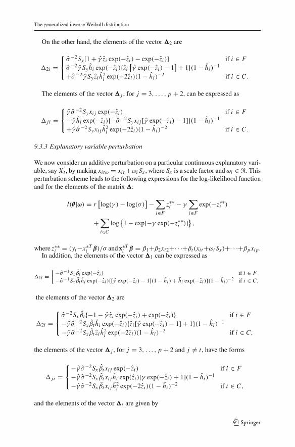
9.3.3 Explanatory variable perturbation

We now consider an additive perturbation on a particular continuous explanatory vari-able, say Xt , by making xitω = xit +ωi Sx , where Sx is a scale factor and ωi ∈ �. Thisperturbation scheme leads to the following expressions for the log-likelihood functionand for the elements of the matrix �:

l(θ |ω) = r[log(γ ) − log(σ )

]−∑i∈F

z∗∗i − γ

∑i∈F

exp(−z∗∗i )

+∑i∈C

log{1 − exp[−γ exp(−z∗∗

i )]} ,

where z∗∗i = (yi −x∗T

i β)/σ and x∗Ti β = β1+β2xi2+· · ·+βt (xit+ωi Sx )+· · ·+βpxip.

In addition, the elements of the vector �1 can be expressed as

�1i ={−σ−1Sx βt exp(−zi ) if i ∈ F

−σ−1Sx βt hi exp(−zi ){[γ exp(−zi ) − 1](1 − hi ) + hi exp(−zi )}(1 − hi )−2 if i ∈ C,

the elements of the vector �2 are

�2i =⎧⎨⎩

σ−2Sx βt {−1 − γ zi exp(−zi ) + exp(−zi )} if i ∈ F−γ σ−2Sx βt hi exp(−zi ){zi [γ exp(−zi ) − 1] + 1}(1 − hi )

−1

−γ σ−2Sx βt zi h2i exp(−2zi )(1 − hi )

−2 if i ∈ C,

the elements of the vector � j , for j = 3, . . . , p + 2 and j �= t , have the forms

� j i =⎧⎨⎩

−γ σ−2Sx βt xi j exp(−zi ) if i ∈ F−γ σ−2Sx βt xi j hi exp(zi )[γ exp(−zi ) + 1](1 − hi )

−1

−γ σ−2Sx βt xi j h2i exp(−2zi )(1 − hi )

−2 if i ∈ C,

and the elements of the vector �t are given by

123

F. R. S. de Gusmão et al.

�ti=

⎧⎪⎨⎪⎩

σ−1Sx

[1 − γ σ−1βt xi t exp(−zi ) − exp(−zi )

]if i ∈ F

−γ σ−1Sx hi exp(−zi ){σ−1βt xi t [γ exp(−zi ) − 1] − 1}(1 − hi )−1

−γ σ−2Sx βt xi j h2i exp(−2zi )(1 − hi )

−2 if i ∈ C.

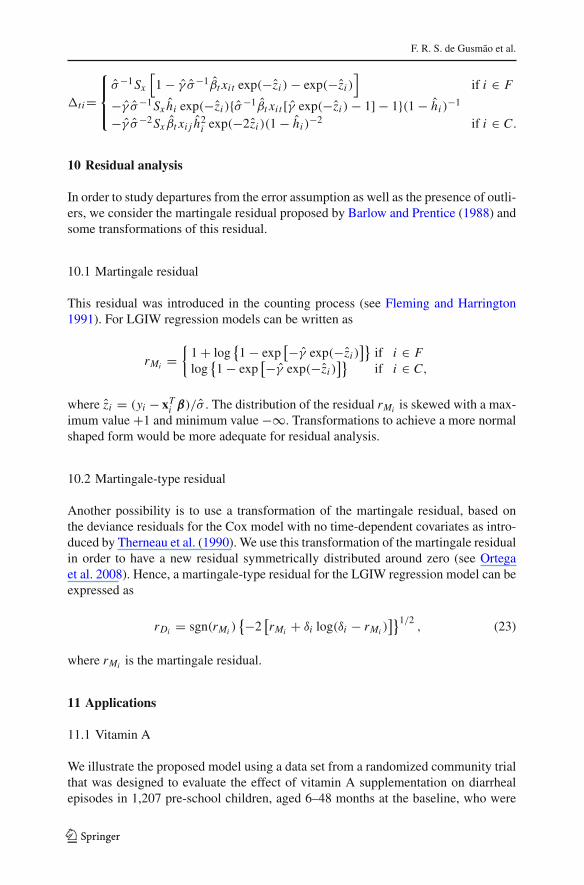
10 Residual analysis

In order to study departures from the error assumption as well as the presence of outli-ers, we consider the martingale residual proposed by Barlow and Prentice (1988) andsome transformations of this residual.

10.1 Martingale residual

This residual was introduced in the counting process (see Fleming and Harrington1991). For LGIW regression models can be written as

rMi ={

1 + log{1 − exp

[−γ exp(−zi )]}

if i ∈ Flog{1 − exp

[−γ exp(−zi )]}

if i ∈ C,

where zi = (yi − xTi β)/σ . The distribution of the residual rMi is skewed with a max-

imum value +1 and minimum value −∞. Transformations to achieve a more normalshaped form would be more adequate for residual analysis.

10.2 Martingale-type residual

Another possibility is to use a transformation of the martingale residual, based onthe deviance residuals for the Cox model with no time-dependent covariates as intro-duced by Therneau et al. (1990). We use this transformation of the martingale residualin order to have a new residual symmetrically distributed around zero (see Ortegaet al. 2008). Hence, a martingale-type residual for the LGIW regression model can beexpressed as

rDi = sgn(rMi ){−2

[rMi + δi log(δi − rMi )

]}1/2, (23)

where rMi is the martingale residual.

11 Applications

11.1 Vitamin A

We illustrate the proposed model using a data set from a randomized community trialthat was designed to evaluate the effect of vitamin A supplementation on diarrhealepisodes in 1,207 pre-school children, aged 6–48 months at the baseline, who were

123

The generalized inverse Weibull distribution

0

0,2

0,4

0,6

0,8

1

0,4 0,80 0,2 0,6 1

i / n

T T

T

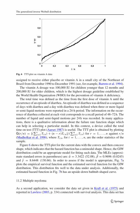
Fig. 6 TTT-plot on vitamin A data

assigned to receive either placebo or vitamin A in a small city of the Northeast ofBrazil from December 1990 to December 1991 (see, for example, Barreto et al. 1994).

The vitamin A dosage was 100,000 IU for children younger than 12 months and200,000 IU for older children, which is the highest dosage guideline established bythe World Health Organization (WHO) for the prevention of vitamin A deficiency.

The total time was defined as the time from the first dose of vitamin A until theoccurrence of an episode of diarrhea. An episode of diarrhea was defined as a sequenceof days with diarrhea and a day with diarrhea was defined when three or more liquidor semi-liquid motions were reported in a 24-h period. The information on the occur-rence of diarrhea collected at each visit corresponds to a recall period of 48–72 h. Thenumber of liquid and semi-liquid motions per 24 h was recorded. In many applica-tions, there is a qualitative information about the failure rate function shape whichcan help in selecting a particular model. In this context, a device called the totaltime on test (TTT) plot (Aarset 1987) is useful. The TTT plot is obtained by plottingG(r/n) = [(∑r

i=1 Ti :n) + (n − r)Tr :n]/(∑ni=1 Ti :n) for r = 1, . . . , n against r/n

(Mudholkar et al. 1996), where Ti :n , for i = 1, . . . , n, are the order statistics of thesample.

Figure 6 shows the TTT-plot for the current data with the convex and then concaveshape, which indicates that the hazard function has a unimodal shape. Hence, the GIWdistribution could be an appropriate model for fitting such data. The MLEs (approxi-mate standard errors in parentheses) are: α = 3.3422 (52.08), β = 0.9696 (0.0245)

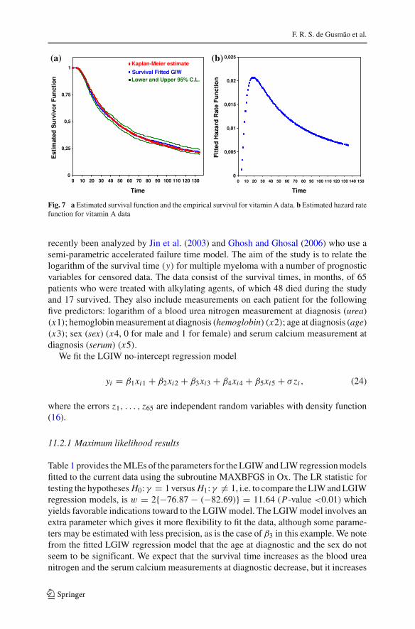
and γ = 8.6448 (130.66). In order to assess if the model is appropriate, Fig. 7aplots the empirical survival function and the estimated survival function for the GIWdistribution. This distribution fits well to the data under analysis. Additionally, theestimated hazard function in Fig. 7b has an upside-down bathtub-shaped curve.

11.2 Multiple myeloma

As a second application, we consider the data set given in Krall et al. (1975) andreported in Lawless (2003, p. 334) connected with survival analysis. This data set has

123

F. R. S. de Gusmão et al.

(a) (b)

0

0,25

0,5

0,75

1

100 110 120 130

Time

Est

imat

ed S

urv

ivo

r F

un

ctio

n

Survival Fitted GIW

Kaplan-Meier estimate

Lower and Upper 95% C.L.

0

0,005

0,01

0,015

0,02

0,025

0 10 20 30 40 50 60 70 80 90 0 10 20 30 40 50 60 70 80 90 100 110 120 130 140 150

TiTime

Fit

ted

Haz

ard

Rat

e F

un

ctio

n

Fig. 7 a Estimated survival function and the empirical survival for vitamin A data. b Estimated hazard ratefunction for vitamin A data

recently been analyzed by Jin et al. (2003) and Ghosh and Ghosal (2006) who use asemi-parametric accelerated failure time model. The aim of the study is to relate thelogarithm of the survival time (y) for multiple myeloma with a number of prognosticvariables for censored data. The data consist of the survival times, in months, of 65patients who were treated with alkylating agents, of which 48 died during the studyand 17 survived. They also include measurements on each patient for the followingfive predictors: logarithm of a blood urea nitrogen measurement at diagnosis (urea)(x1); hemoglobin measurement at diagnosis (hemoglobin) (x2); age at diagnosis (age)(x3); sex (sex) (x4, 0 for male and 1 for female) and serum calcium measurement atdiagnosis (serum) (x5).

We fit the LGIW no-intercept regression model

yi = β1xi1 + β2xi2 + β3xi3 + β4xi4 + β5xi5 + σ zi , (24)

where the errors z1, . . . , z65 are independent random variables with density function(16).

11.2.1 Maximum likelihood results

Table 1 provides the MLEs of the parameters for the LGIW and LIW regression modelsfitted to the current data using the subroutine MAXBFGS in Ox. The LR statistic fortesting the hypotheses H0: γ = 1 versus H1: γ �= 1, i.e. to compare the LIW and LGIWregression models, is w = 2{−76.87 − (−82.69)} = 11.64 (P-value <0.01) whichyields favorable indications toward to the LGIW model. The LGIW model involves anextra parameter which gives it more flexibility to fit the data, although some parame-ters may be estimated with less precision, as is the case of β3 in this example. We notefrom the fitted LGIW regression model that the age at diagnostic and the sex do notseem to be significant. We expect that the survival time increases as the blood ureanitrogen and the serum calcium measurements at diagnostic decrease, but it increases

123

The generalized inverse Weibull distribution

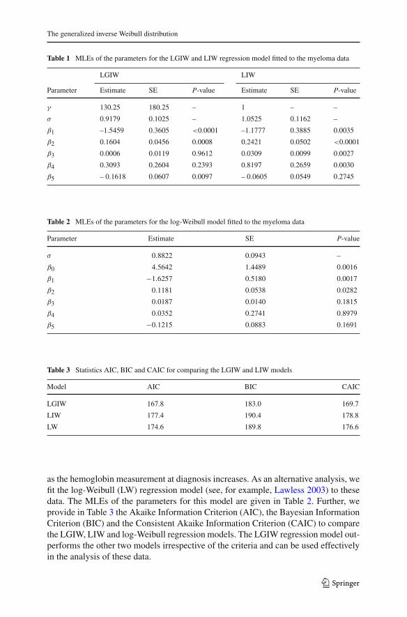
Table 1 MLEs of the parameters for the LGIW and LIW regression model fitted to the myeloma data

LGIW LIW

Parameter Estimate SE P-value Estimate SE P-value

γ 130.25 180.25 – 1 – –

σ 0.9179 0.1025 – 1.0525 0.1162 –

β1 –1.5459 0.3605 <0.0001 –1.1777 0.3885 0.0035

β2 0.1604 0.0456 0.0008 0.2421 0.0502 <0.0001

β3 0.0006 0.0119 0.9612 0.0309 0.0099 0.0027

β4 0.3093 0.2604 0.2393 0.8197 0.2659 0.0030

β5 – 0.1618 0.0607 0.0097 – 0.0605 0.0549 0.2745

Table 2 MLEs of the parameters for the log-Weibull model fitted to the myeloma data

Parameter Estimate SE P-value

σ 0.8822 0.0943 –

β0 4.5642 1.4489 0.0016

β1 −1.6257 0.5180 0.0017

β2 0.1181 0.0538 0.0282

β3 0.0187 0.0140 0.1815

β4 0.0352 0.2741 0.8979

β5 −0.1215 0.0883 0.1691

Table 3 Statistics AIC, BIC and CAIC for comparing the LGIW and LIW models

Model AIC BIC CAIC

LGIW 167.8 183.0 169.7

LIW 177.4 190.4 178.8

LW 174.6 189.8 176.6

as the hemoglobin measurement at diagnosis increases. As an alternative analysis, wefit the log-Weibull (LW) regression model (see, for example, Lawless 2003) to thesedata. The MLEs of the parameters for this model are given in Table 2. Further, weprovide in Table 3 the Akaike Information Criterion (AIC), the Bayesian InformationCriterion (BIC) and the Consistent Akaike Information Criterion (CAIC) to comparethe LGIW, LIW and log-Weibull regression models. The LGIW regression model out-performs the other two models irrespective of the criteria and can be used effectivelyin the analysis of these data.

123

F. R. S. de Gusmão et al.

(a) (b)

0

10

20

30

40

50

60

10 15 20 25 30 35 40 45 50 55 60 65

Index

Gen

eral

ized

Coo

k D

ista

nce

5

0

2

4

6

10 15 20 25 30 35 40 45 50 55 60 65

Index

Like

lihoo

d D

ista

nce

5

40

12

0 5 0 5

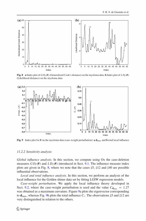
Fig. 8 a Index plot of G Di (θ) (Generalized Cook’s distance) on the myeloma data. b Index plot of L Di (θ)

(Likelihood distance) on the myeloma data

(a) (b)

-0,8

-0,7

-0,6

-0,5

-0,4

-0,3

-0,2

-0,1

0

0,1

0,2

0,3

0 5 10 15 20 25 30 35 40 45 50 55 60 65

Index

d m

axi( θ

)

5 0

0,12

0,24

0,36

0,48

0,6

0,72

0 5 10 15 20 25 30 35 40 45 50 55 60 65

Index

5

C i

( θ)

12

Fig. 9 Index plot for θ on the myeloma data (case-weight perturbation): a dmax and b total local influence

11.2.2 Sensitivity analysis

Global influence analysis. In this section, we compute using Ox the case-deletionmeasures G Di (θ) and L Di (θ) introduced in Sect. 9.1. The influence measure indexplots are given in Fig. 8, where we note that the cases �5, �12 and �40 are possibleinfluential observations.

Local and total influence analysis. In this section, we perform an analysis of thelocal influence for the Golden shiner data set by fitting LGIW regression models.

Case-weight perturbation. We apply the local influence theory developed inSect. 9.2, where the case-weight perturbation is used and the value Cdmax = 1.27was obtained as a maximum curvature. Figure 9a plots the eigenvector correspondingto dmax, whereas Fig. 9b plots the total influence Ci . The observations �5 and �12 arevery distinguished in relation to the others.

123

The generalized inverse Weibull distribution

(a) (b)

-0,6

-0,5

-0,4

-0,3

-0,2

-0,1

0

0,1

0 5 10 15 20 25 30 35 40 45 50 55 60 65

Index

d m

axi( θ

)

12

5

0

1

2

3

4

5

6

7

8

0 5 10 15 20 25 30 35 40 45 50 55 60 65Index

5

C i ( θ

)

12

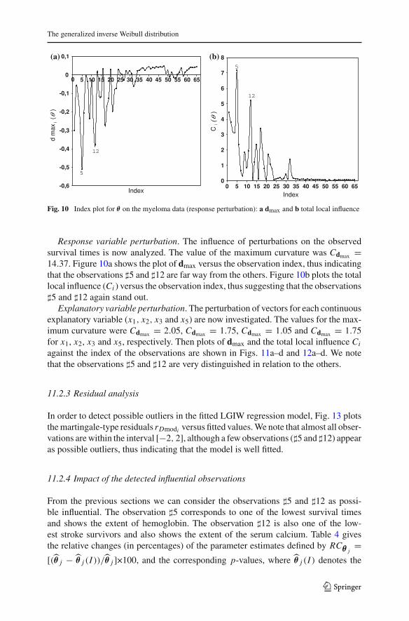
Fig. 10 Index plot for θ on the myeloma data (response perturbation): a dmax and b total local influence

Response variable perturbation. The influence of perturbations on the observedsurvival times is now analyzed. The value of the maximum curvature was Cdmax =14.37. Figure 10a shows the plot of dmax versus the observation index, thus indicatingthat the observations �5 and �12 are far way from the others. Figure 10b plots the totallocal influence (Ci ) versus the observation index, thus suggesting that the observations�5 and �12 again stand out.

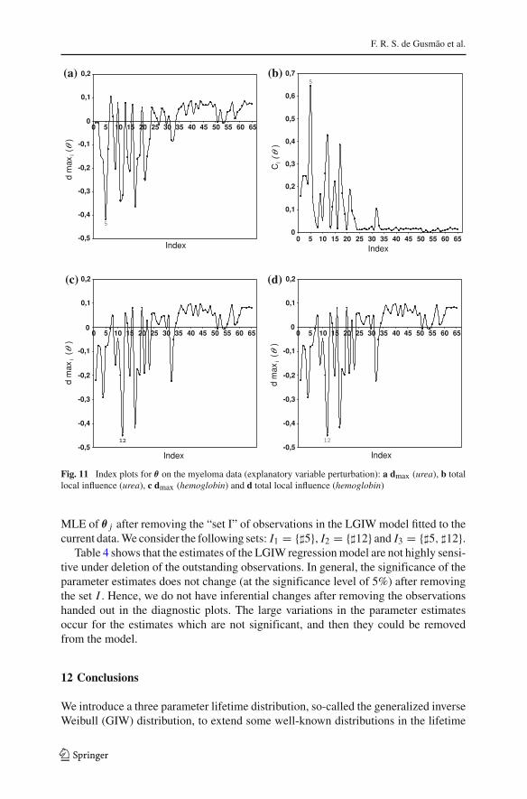
Explanatory variable perturbation. The perturbation of vectors for each continuousexplanatory variable (x1, x2, x3 and x5) are now investigated. The values for the max-imum curvature were Cdmax = 2.05, Cdmax = 1.75, Cdmax = 1.05 and Cdmax = 1.75for x1, x2, x3 and x5, respectively. Then plots of dmax and the total local influence Ci

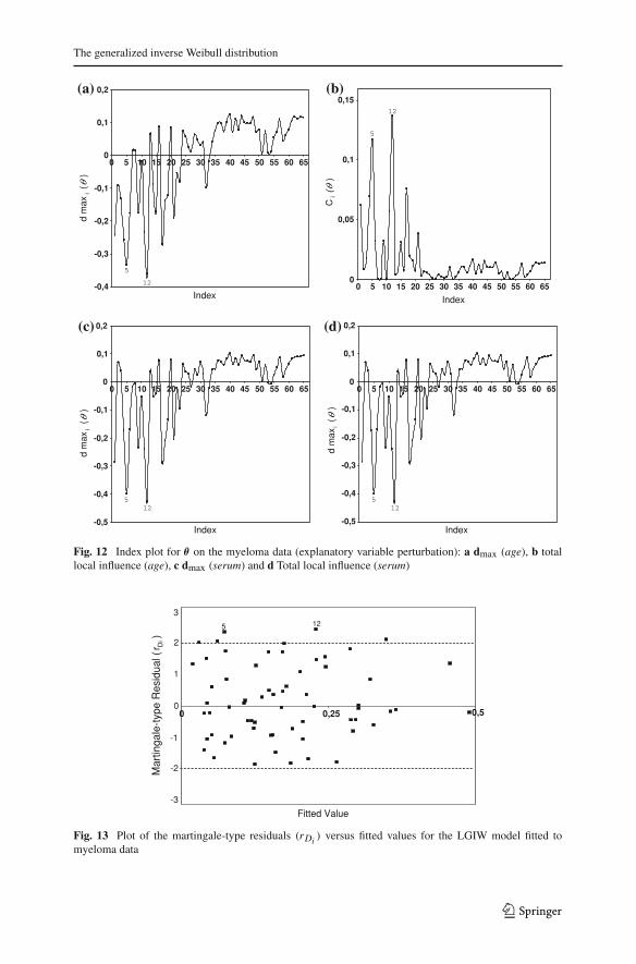
against the index of the observations are shown in Figs. 11a–d and 12a–d. We notethat the observations �5 and �12 are very distinguished in relation to the others.

11.2.3 Residual analysis

In order to detect possible outliers in the fitted LGIW regression model, Fig. 13 plotsthe martingale-type residuals rDmodi versus fitted values. We note that almost all obser-vations are within the interval [−2, 2], although a few observations (�5 and �12) appearas possible outliers, thus indicating that the model is well fitted.

11.2.4 Impact of the detected influential observations

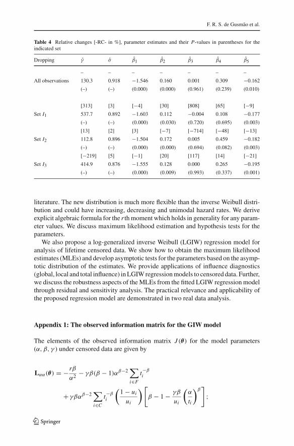
From the previous sections we can consider the observations �5 and �12 as possi-ble influential. The observation �5 corresponds to one of the lowest survival timesand shows the extent of hemoglobin. The observation �12 is also one of the low-est stroke survivors and also shows the extent of the serum calcium. Table 4 givesthe relative changes (in percentages) of the parameter estimates defined by RCθ j

=[(θ j − θ j (I ))/θ j ]×100, and the corresponding p-values, where θ j (I ) denotes the

123

F. R. S. de Gusmão et al.

(a) (b)

-0,5

-0,4

-0,3

-0,2

-0,1

0

0,1

0,2

10 15 20 25 30 35 40 45 50 55 60 65

Index

d m

axi(θ

)

5

0

0,1

0,2

0,3

0,4

0,5

0,6

0,7

10 15 20 25 30 35 40 45 50 55 60 65Index

5

C i (

θ)

(c) (d)

-0,5

-0,4

-0,3

-0,2

-0,1

0

0,1

0,2

10 15 20 25 30 35 40 45 50 55 60 65

Index

d m

axi

( θ)

1212-0,5

-0,4

-0,3

-0,2

-0,1

0

0,1

0,2

0 5

0 5

0 5 0 5 10 15 20 25 30 35 40 45 50 55 60 65

Index

d m

axi

( θ)

12

Fig. 11 Index plots for θ on the myeloma data (explanatory variable perturbation): a dmax (urea), b totallocal influence (urea), c dmax (hemoglobin) and d total local influence (hemoglobin)

MLE of θ j after removing the “set I” of observations in the LGIW model fitted to thecurrent data. We consider the following sets: I1 = {�5}, I2 = {�12} and I3 = {�5, �12}.

Table 4 shows that the estimates of the LGIW regression model are not highly sensi-tive under deletion of the outstanding observations. In general, the significance of theparameter estimates does not change (at the significance level of 5%) after removingthe set I . Hence, we do not have inferential changes after removing the observationshanded out in the diagnostic plots. The large variations in the parameter estimatesoccur for the estimates which are not significant, and then they could be removedfrom the model.

12 Conclusions

We introduce a three parameter lifetime distribution, so-called the generalized inverseWeibull (GIW) distribution, to extend some well-known distributions in the lifetime

123

The generalized inverse Weibull distribution

(a) (b)

-0,4

-0,3

-0,2

-0,1

0

0,1

0,2

10 15 20 25 30 35 40 45 50 55 60 65

Index

d m

axi

( θ)

12

5

0

0,05

0,1

0,15

10 15 20 25 30 35 40 45 50 55 60 65

Index

5

C i ( θ

)

12

(c) (d)

-0,5

-0,4

-0,3

-0,2

-0,1

0

0,1

0,2

10 15 20 25 30 35 40 45 50 55 60 65

Index

12

d m

axi

( θ)

5

-0,5

-0,4

-0,3

-0,2

-0,1

0

0,1

0,2

0 5

0 5

0 5 0 5 10 15 20 25 30 35 40 45 50 55 60 65

Index

12

d m

axi

( θ)

5

Fig. 12 Index plot for θ on the myeloma data (explanatory variable perturbation): a dmax (age), b totallocal influence (age), c dmax (serum) and d Total local influence (serum)

0,250 0,5

Fitted Value

Mar

tinga

le-t

ype

Res

idua

l ( r D

i)

5 123

2

1

0

-1

-2

-3

Fig. 13 Plot of the martingale-type residuals (rDi ) versus fitted values for the LGIW model fitted tomyeloma data

123

F. R. S. de Gusmão et al.

Table 4 Relative changes [-RC- in %], parameter estimates and their P-values in parentheses for theindicated set

Dropping γ σ β1 β2 β3 β4 β5

– – – – – – –

All observations 130.3 0.918 −1.546 0.160 0.001 0.309 −0.162

(–) (–) (0.000) (0.000) (0.961) (0.239) (0.010)

[313] [3] [−4] [30] [808] [65] [−9]

Set I1 537.7 0.892 −1.603 0.112 −0.004 0.108 −0.177

(–) (–) (0.000) (0.030) (0.720) (0.695) (0.003)

[13] [2] [3] [−7] [−714] [−48] [−13]

Set I2 112.8 0.896 −1.504 0.172 0.005 0.459 −0.182

(–) (–) (0.000) (0.000) (0.694) (0.082) (0.003)

[−219] [5] [−1] [20] [117] [14] [−21]

Set I3 414.9 0.876 −1.555 0.128 0.000 0.265 −0.195

(–) (–) (0.000) (0.009) (0.993) (0.337) (0.001)

literature. The new distribution is much more flexible than the inverse Weibull distri-bution and could have increasing, decreasing and unimodal hazard rates. We deriveexplicit algebraic formula for the r th moment which holds in generality for any param-eter values. We discuss maximum likelihood estimation and hypothesis tests for theparameters.

We also propose a log-generalized inverse Weibull (LGIW) regression model foranalysis of lifetime censored data. We show how to obtain the maximum likelihoodestimates (MLEs) and develop asymptotic tests for the parameters based on the asymp-totic distribution of the estimates. We provide applications of influence diagnostics(global, local and total influence) in LGIW regression models to censored data. Further,we discuss the robustness aspects of the MLEs from the fitted LGIW regression modelthrough residual and sensitivity analysis. The practical relevance and applicability ofthe proposed regression model are demonstrated in two real data analysis.

Appendix 1: The observed information matrix for the GIW model

The elements of the observed information matrix J (θ) for the model parameters(α, β, γ ) under censored data are given by

Lαα(θ) = −rβ

α2 − γβ(β − 1)αβ−2∑i∈F

t−βi

+ γβαβ−2∑i∈C

t−βi

(1 − ui

ui

)[β − 1 − γβ

ui

(α

ti

)β]

;

123

The generalized inverse Weibull distribution

Lαβ(θ) = r

α− γαβ−1

∑i∈F

t−βi

[1 + β log

(α

ti

)]

+ γαβ−1∑i∈C

t−βi

(1 − ui

ui

){1 + β log

(α

ti

)[1 − γ

ui

(α

ti

)β]}

;

Lγβ(θ)=−αβ∑i∈F

t−βi log

(α

ti

)+αβ

∑i∈C

t−βi log

(α

ti

)(1−ui

ui

)[1− γ

ui

(α

ti

)β]

;

Lαγ (θ) = −βαβ−1∑i∈F

t−βi + βαβ−1

∑i∈C

t−βi

(1 − ui

ui

)[1 − γ

ui

(α

ti

)β]

;

Lγ γ (θ) = − r

γ 2 − α2β∑i∈C

t−2βi

(1 − ui

u2i

);

and

Lββ(θ) = − r

β2 − γαβ∑i∈F

log

(α

ti

)[log(α) − t−β

i log(ti )]

+ γαβ∑i∈C

log

(α

ti

)(1 − ui

ui

)[log(α) − t−β

i log(ti )

− t−βi γ

ui

(α

ti

)β

log

(α

ti

)].

Here, ui = 1 − exp

[−γ(

αti

)β]

.

Appendix 2: The observed information matrix for the LGIW model

We derive the second-order partial derivatives of the log-likelihood function. Aftersome algebraic manipulations, we obtain

Lγ γ = − r

σ 2 −∑i∈C

exp(−2zi )hi (1 − hi )−2;

Lγ σ =∑i∈F

exp(−zi )(zi )σ +∑i∈C

hi exp(−zi )(zi )σ [γ exp(−zi )](1 − hi )−1

+∑i∈C

h2i γ exp(−2zi )(zi )σ (1 − h−2

i );

123

F. R. S. de Gusmão et al.

Lγβ j =∑i∈F

exp(−zi )(zi )β j +∑i∈C

hi exp(−zi )(zi )β j [γ exp(−zi )](1 − hi )−1

+∑i∈C

h2i γ exp(−2zi )(zi )β j (1 − h−2

i );

Lσσ = r

σ 2 +∑i∈F

{−(zi )σσ + γ exp(−zi )

[− [(zi )σ ]2 + (zi )σσ

]}

−γ∑i∈C

hi exp(−zi ){

[(zi )σ ]2 [γ exp(−zi ) − 1] + (zi )σσ

}(1 − hi )

−1

−γ∑i∈C

h2i exp(−2zi ) [(zi )σ ]2 (1 − hi )

−2;

Lσβ j = −∑i∈F

(zi )β j σ + γ∑i∈F

[− exp(−zi )(zi )β j (zi )σ + exp(−zi )(zi )β j σ

]

−γ∑i∈C

hi exp(−zi ){(zi )β j (zi )σ [γ exp(−zi ) − 1] + (zi )β j σ

}(1 − hi )

−1

+ γ∑i∈C

h2i exp(−2zi )(zi )β− j (zi )σ (1 − hi )

−2;

and

Lβ j βs =∑i∈F

[−γ exp(−zi )(zi )β j (zi )βs

]

−γ∑i∈C

hi exp(−zi ){(zi )β j (zi )βs [γ exp(−zi ) − 1]} (1 − hi )

−1

−γ∑i∈C

h2i exp(−2zi )(zi )β j (zi )βs (1 − hi )

−2;

where hi = exp[−γ exp(−zi )], (zi )σ = −zi/σ , (zi )β j = −xi j/σ , (zi )βs = −xis/σ ,(zi )σσ = 2zi/σ

2, (zi )β j σ = xi j/σ2 and zi = (yi − xT

i β)/σ .

References

Aarset MV (1987) How to identify bathtub hazard rate. IEEE Trans Reliab 36:106–108AL-Hussaini EK, Sultan KS (2001) Reliability and hazard based on finite mixture models. In: Balakrishnan

N, Rao CR (eds) Handbook of statistics, vol 20. Elsevier, Amsterdam pp 139–183Barakat HM, Abdelkader YH (2004) Computing the moments of order statistics from nonidentical random

variables. Stat Methods Appl 13:15–26Barlow WE, Prentice RL (1988) Residuals for relative risk regression. Biometrika 75:65–74Barreto ML, Santos LMP, Assis AMO, Araújo MPN, Farenzena GG, Santos PAB, Fiaccone

RL (1994) Effect of vitamin A supplementation on diarrhoea and acute lower-respiratory-tract infec-tions in young children in Brazil. Lancet 344:228–231

Chandra S (1977) On the mixtures of probability distributions. Scand J Stat 4:105–112Cook RD (1986) Assesment of local influence (with discussion). J R Stat Soc B 48:133–169Doornik J (2007) Ox: an object-oriented matrix programming language. International Thomson Bussiness

Press, London

123

The generalized inverse Weibull distribution

Drapella A (1993) Complementary Weibull distribution: unknown or just forgotten. Qual Reliab Eng Int9:383–385

Everitt BS, Hand DJ (1981) Finite mixture distributions. Chapman and Hall, LondonFleming TR, Harrington DP (1991) Counting process and survival analysis. Wiley, New YorkGhosh SK, Ghosal S (2006) Semiparametric accelerated failure time models for censored data. In: Upad-

hyay SK, Singh U, Dey DK (eds) Bayesian statistics and its applications. Anamaya Publishers,New Delhi pp 213–229

Hosmer DW, Lemeshow S (1999) Applied survival analysis. Wiley, New YorkJiang R, Zuo MJ, Li HX (1999) Weibull and Weibull inverse mixture models allowing negative weights.

Reliab Eng Syst Saf 66:227–234Jiang R, Murthy DNP, Ji P (2001) Models involving two inverse Weibull distributions. Reliab Eng Syst Saf

73:73–81Jin Z, Lin DY, Wei LJ, Ying Z (2003) Rank-based inference for the accelerated failure time model. Bio-

metrika 90:341–353Keller AZ, Kamath AR (1982) Reliability analysis of CNC machine tools. Reliab Eng 3:449–473Krall J, Uthoff V, Harley J (1975) A step-up procedure for selecting variables associated with survival.

Reliab Eng Syst Saf 73:73–81Lawless JF (2003) Statistical models and methods for lifetime data. Wiley, New YorkLesaffre E, Verbeke G (1998) Local influence in linear mixed models. Biometrics 54:570–582Maclachlan GJ, Krishnan T (1997) The EM algorithm and extensions. Wiley, New YorkMaclachlan G, Peel D (2000) Finite mixture models. Wiley, New YorkMudholkar GS, Kollia GD (1994) Generalized Weibull family: a structural analysis. Commun Stat Ser A

23:1149–1171Mudholkar GS, Srivastava DK, Kollia GD (1996) A generalization of the Weibull distribution with appli-

cation to the analysis of survival data. J Am Stat Assoc 91:1575–1583Nadarajah S (2006) The exponentiated Gumbel distribution with climate application. Environmetrics

17:13–23Ortega EMM, Paula GA, Bolfarine H (2008) Deviance residuals in generalized log-gamma regression mod-

els with censored observations. J Stat Comput Simul 78:747–764Prudnikov AP, Brychkov YA, Marichev OI (1986) Integrals and series. Gordon and Breach Science Pub-

lishers, New YorkSultan KS, Ismail MA, Al-Moisheer AS (2007) Mixture of two inverse Weibull distributions: properties

and estimation. Comput Stat Data Anal 51:5377–5387Therneau TM, Grambsch PM, Fleming TR (1990) Martingale-based residuals for survival models. Biomet-

rika 77:147–160

123