A modified Weibull model for bacterial inactivation

www.elsevier.com/locate/ijfoodmicro

International Journal of Food Micro

A modified Weibull model for bacterial inactivation

I. Alberta,*, P. Mafartb

aUnite Met@risk, Institut National Agronomique de Paris-Grignon, 16, rue Claude Bernard 75231 Paris cedex 05, FrancebLaboratoire Universitaire de Microbiologie Appliquee de Quimper, Pole Universitaire de Creach Gwen, 29000 Quimper, France

Received 27 September 2004; accepted 6 October 2004

Abstract

In this paper, a modified Weibull model is proposed to fit microbial survival curves. This model can incorporate shoulder

and/or tailing phenomena if they are encountered. We aim to obtain an accurate fit of the bprimaryQ modelling of the bacterial

inactivation and to provide a useful and meaningful model for biologists and food industry. A d parameter close to the classical

concept of the D value, established for sterilisation processes, is used in the model. The specific parameterisation of the Weibull

model is evaluated for the parameter of interest d. The goodness-of-fit of the model is compared to the one produced by the

model proposed by Geeraerd et al., [Geeraerd, A.H., Herremans, C.H., Van Impe, J.F., 2000. Structural model requirements to

describe microbial inactivation during a mild heat treatment. Int. J. Food Microbiol. 59, 185-209.] on experimental data. As our

model provides good fits for the different types of survival curves analysed, further research can focus on the development of

suitable secondary model types. In this respect, it is interesting to note that the d parameter is close to the D concept.

D 2004 Elsevier B.V. All rights reserved.

Keywords: Predictive microbiology; Primary model; Bacterial inactivation; Survival curves; Heat treatment; Weibull

1. Introduction

Modelling bacterial survival curves becomes more

andmore an important issue due to the increasing use of

mild heat treatments for food products which have to

guarantee the safety of the products and due to the

increasing use of risk analyses aiming at a better control

of the foodborne diseases. Whereas models have been

0168-1605/$ - see front matter D 2004 Elsevier B.V. All rights reserved.

doi:10.1016/j.ijfoodmicro.2004.10.016

* Corresponding author. Tel.: +33 1 4408 7271; fax: +33 1 4408

7276.

E-mail address: [email protected] (I. Albert).

developed during the last 15 years by predictive

microbiology in order to determine microbial growth

in constant and variable environment, useful models

have to be proposed to deal with microbial decrease in

constant and variable environment. Numerous models

have been proposed yet in this scope but many of them

have been developed for very specific needs and cannot

deal with most typical behaviours of microbial survivor

curves. An excellent review on the subject has been

published by Geeraerd et al. (2000).

Most microbial survival curves have a non-log-

linear behaviour. Phenomena such as shoulder

(smooth initiation) and tailing (saturation) of survivor

biology 100 (2005) 197–211

I. Albert, P. Mafart / International Journal of Food Microbiology 100 (2005) 197–211198

curves are frequent. Even if a better insight of those

phenomena has to be found to possibly control them,

a predictive survival model must in any case

incorporate those phenomena if they exist to provide

good parameter estimates by an accurate fit of the

experimental data. Actually, microbial survival curves

have the shape of survival curves described in the

literature of failure time data when distinguishing

individuals (Kalbfleisch and Prentice, 1980; Lawless,

1982). Microbial survival curves are the cumulative of

the individual failure distributions as mentioned

previously by Peleg and Cole (1998). However, the

background of bacterial inactivation is different

because the individual organism failure time is

unknown, the absolute population have to be

described (not the population relative to the initial

population) and because the possibility of a tailing

phenomenon has to be incorporated.

In the context of failure time data analysis,

numerous parametric models have been proposed:

exponential, Weibull, log-normal, log-logistic, gamma,

Pareto distributions for example. Most of those models

are different from each other by their long-term

behaviour but often do not have a non-zero asymptote

to take into account a phenomenon of saturation.

In this paper, we propose a specific parameter-

isation and an extension of the Weibull model to

describe microbial inactivation (Albert and Mafart,

2003) and take into account its features as mentioned

previously.

This paper is organised as follows. In the next

section, experimental data used for fitting the model are

presented, the novel model is introduced and the

methods for the parameter estimation and model eva-

luation are set out. Section 3 deals with the exper-

imental data fits. On the experimental data, the new

model is compared with a model proposed recently by

Geeraerd et al. (2000) for bacterial inactivation and

the re-parameterisation of the Weibull model is

evaluated. We conclude in Section 4 by a discussion.

2. Materials and methods

2.1. Origin of experimental data used

Table 1 gives an overview of the experimental

data used for the fits. Spores and vegetative bacteria

are analysed. All experiments were carried out in

static environmental conditions. 40 curves are

analysed from four strains. The strain of Bacillus

pumilus A40, isolated from eggs powder, were

supplied by Saupiquet (France). The strain of

Bacillus cereus Bce 1, isolated from dairy food line

process, were supplied by Danone (France). The two

strains were studied at Quimper University Research

Department, Laboratoire Universitaire de Microbio-

logie Appliquee (LUMAQ). For more details on the

microorganism and spore production, and the ther-

mal treatment of spore suspension, see Mafart et al.

(2002). The data sets related to Clostridium botu-

linum 213B originate from literature (Anderson et

al., 1996). The data sets from Listeria innocua

ATCC 51742 originate from LUMAQ unpublished

results.

These data sets were selected to explore a large

range of time values (heat treatment duration from 4

to 45.25 min) and microbial population size values

(from 103 to 109 cfu ml�1), and for the shape of their

survivor curves. Survivor curves of B. pumilus and

B. cereus exhibit a bshoulderQ and no tailing

(downward concavity: type A curve, see Fig. 1 for

example) contrary to the C. botulinum curves which

have no shoulder and no tailing (upward concavity:

type B curve, see Fig. 7 for example). The L.

innocua survivor curves were chosen because of

their sigmoidal shape (with a shoulder and a tailing

effect: type C curve, see Fig. 5 for example). The

average number of points by curve is 11.2. The

number of observations by curve ranges from 7 to

18, and replications are sometimes available (data

related to C. botulinum are all repeated two

times).

2.2. The inactivation model

The kinetics of the bacterial population decrease

(cfu ml�1) versus time (min) is described by the

following model:

c t=dð Þ ¼ N0 � Nresð Þ10 � 1dð Þ

pð Þ þ Nres; ð1Þ

where t is time, c(t) is the bacterial concentration at

time t, N0(N0N0), Nres(Nresz0), d(dN0) and p( pN0)

are unknown parameters which have to be estimated.

N0 and Nres represent the unknown values of the

Table 1

Overview of the experimental data used (all experiments were carried out in optimal temperature recovery medium and optimal aw recovery

medium)

Data source (number

of curves analysed)

Isolated

from

Data set

number

T (8C)treatment

medium

pH

treatment

medium

aw

treatment

medium

pH

recovery

medium

Number of points by

curve (possibly

number of repetitions)

Bacillus pumilus A40 (9)

(Mafart et al., 2002)

egg powder Bp1 98 7 0.997 7 12

Bp2 95 7 0.997 5.82 12

Bp3 95 7 0.997 6.04 13

Bp4 92 7 0.997 7 9

Bp5 95 7 0.997 7 18 (1 repetition)

Bp6 95 7 0.997 6.26 13

Bp7 95 7 0.997 7.15 12

Bp8 95 7 0.997 7.83 11

Bp9 95 7 0.997 8.82 12

Bacillus cereus Bce 1 (8)

(Mafart et al., 2002)

dairy food Bc1 95 3 0.997 7 13

Bc2 96 4 0.98 7 12

Bc3 90 5.5 0.997 7 11

Bc4 100 5.5 0.95 7 12

Bc5 95 3.5 0.947 7 10

Bc6 95 3.84 0.997 7 8

Bc7 95 3.39 0.997 7 7

Bc8 95 5.56 0.997 7 8

Clostridium botulinum

213B (5) (Anderson

et al., 1996)

cooked meat Cb1 101 7 0.997 7 14 (7 repetitions)

Cb2 103 7 0.997 7 14 (7 repetitions)

Cb3 105 7 0.997 7 12 (6 repetitions)

Cb4 109 7 0.997 7 14 (7 repetitions)

Cb5 111 7 0.997 7 14 (7 repetitions)

Listeria innocua ATCC

51742 (18)

(Unpublished results

from LUMAQ)

Li1 55 6.83 0.997 6.94 12

Li2 55 6.83 0.997 6.5 11

Li3 55 6.83 0.997 6.05 12

Li4 55 6.83 0.997 5.5 13

Li5 55 6.83 0.997 5.13 10

Li6 55 6.48 0.997 6.88 11

Li7 55 6.48 0.997 5.48 8

Li8 55 6 0.997 6.88 10

Li9 55 6 0.997 6.5 10

Li10 55 6 0.997 6 9

Li11 55 6 0.997 5.5 10

Li12 55 5.5 0.997 6.5 10

Li13 55 5.5 0.997 6 10

Li14 55 5.5 0.997 5.5 10

Li15 55 5 0.997 6 11

Li16 55 5 0.997 5.5 10

Li17 55 5 0.997 5 10

Li18 55 4.5 0.997 6.5 10

I. Albert, P. Mafart / International Journal of Food Microbiology 100 (2005) 197–211 199

initial bacterial concentration (at time t=0) and the

residual bacterial concentration (at the end of the

observation), respectively. Nres does not measure the

value of bacterial concentration at t=l. It will be

certainly zero! It has just ambition to allow the fit of

the sigmoidal curve observed in the bacterial inacti-

vation process. In the article of Geeraerd et al. (2000),

possible interpretations of Nres are given. The dparameter represents the time of the first decimal

reduction concentration for the part of the population

not belonging to Nres. In Eq. (1), if t=d we have:

c dð Þ � Nres

N0 � Nres

¼ 1

10: ð2Þ

Fig. 1. A semi-logarithmic plot of the fits from Eqs. (1) and (9) to the raw data set Bp1, shown as log10cfu ml�1 vs. time (min).


Model (Eq. (1)) is close to the model proposed by

Peleg and Cole (1998):

logc tð ÞN0

� �¼ � kt P: ð3Þ

Nevertheless, the model we propose is different from

it because in Eq. (1), a possible tailing effect is

modelled and another parameterisation of Eq. (3) is

introduced with:

d ¼ 1

k

� �1=p

ð4Þ

The p parameter allows to bcatchQ the curve

concavity or convexity. If 0bpb1, the curve has no

inflexion point and hence no shoulder. If pN1,

the curve has an inflexion point and hence

permits a shoulder effect (with a tailing if

Nresp 0). If p=1, the decrease is log-linear and

it corresponds to a first-order decay reaction (if

Nres=0) (Chick, 1908).

Our model has unquestionable advantages:

(i) It permits the fit of most typical survivor curves

(types A, B and C) because it stems from a very

flexible survival model, the well-known Weibull

model.

(ii) The model is parsimonious with only four

parameters or three if Nres is not necessary

(assumed to be equal to zero when no tailing).

(iii) Its parameters are meaningful. In particular, we

use a d parameter whose meaning is close to the

one of the D parameter well-known by biolo-

gists and food industry. This parameter could be

the starting point of a bsecondaryQ modelling as

suggested by Bigelow (1921) (for the D value)

and Mafart et al. (2001). Even if the p parameter

has no direct biological interpretation, its role on

the curve shape is obvious.

Finally, note that our model has the structural

model requirements to describe microbial inactivation

that are listed by Geeraerd et al. (2000):

– the model representing the bacterial population

decrease as a function of time can simulate a

shoulder, a tail or both and encompasses loglinear

inactivation (when p=1 and Nres=0).

– A model dynamic version can be written as

follows:

dcdt

¼ � ln 10ð Þdp

pt p�1 1� Nres

c

� �c: ð5Þ


To fit the experimental data sets, the following

statistical regression model is assumed: the observed

bacterial concentration (unit: cfu ml�1) at time t, N(t),

is written as:

N tð Þ ¼ c tð Þ þ e tð Þ; ð6Þ

where c(t) describes the relationship between the

observed bacterial concentration and the time t (Eq.

(1)). e(t) is the discrepancy between the observation

N(t) and its expectation c(t). The errors e(t) (0VtVtn,where tn is the last time of observation) are centred

random variables (E[e(t)]=0). The errors are assumed

to be independent. Moreover, to complete the

regression model, a variance model is introduced

assuming that the variance of e(t), denoted by rt2,

exists and equals:

r2t ¼ r2c tð Þq; ð7Þ

where r2 and q have to be estimated. A value of q

equals to 2 means that the logarithmic transformation

of the responses stabilises the error variances and a

value of q equals to 1 means that the square-root

transformation of the responses stabilises the error

variances. When the observations are counts, it is

frequent to observe that the variability of the response

depends on its level (Seber and Wild, 1989, pp. 68–

89). This phenomenon is found in predictive micro-

biology. In most models, a logarithmic or square-root

transformation of the responses is done to stabilise the

error variances. Here, we do not choose this systematic

transformation. Our variance modelling is much more

flexible. It generalises the usual models. It requires the

estimation of a supplementary parameter q but allows

to take into account a variance heterogeneity much

more adapted to the observations. A bad variance

stabilisation may lead to wrong parameter estimates

and parameter variances estimates.

In addition, several authors choose to model the

population relative to the initial population, N(t)/N0, in

place of the absolute population N(t). More precisely,

they replace the unknown N0 by an estimate based on

the observations in t=0. Generally, the number of

replications is small and therefore the estimate of N0 is

very poor. As a consequence, the estimation of the

parameters of the kinetics are biased and their variance

is underestimated. Considering the statistical model

defined by Eq. (6) overcomes these drawbacks and

allows to estimate N0 with a greater precision because

all the observations contribute to its estimation.

2.3. Parameter estimation and model evaluation

Nonlinear regressions were performed on the

survival data using the nls2 procedure in S-PLUS

(Insightful, Seattle, WA, USA) developed in our

department, available on the website: http://www.

inra.fr/bia/J/AB/nls2. A book is published to explain

the statistical methods used and includes examples of

use of nls2 (Huet et al., 2003). The important

advantage of the nls2 function is that heteroscedas-

ticity of errors can be taken into account and

estimated by modelling the variance function.

To estimate the parameters, the maximum like-

lihood method assuming Gaussian observations is

used. We chose this method to have an objective

criterion, a likelihood model value, to compare our

model to another non-nested model (the Geeraerd et

al.’s model, see below). Other approaches are possi-

ble. The quasi-likelihood method (Huet et al., 2003)

or an iterated two-stage least squares method (Seber

and Wild, 1989) could be used. The use of weighted

least squares is not possible because the estimators of

this approach are not consistent (they are asymptoti-

cally biased) in the context of a parametric modelling

of the variance.

The complete model depends on six parameters (d,p, N0, Nres, q and r2). In nonlinear regression models,

the maximum likelihood estimator values cannot be

given explicitly (as well as the least squares estimator

values) and are obtained by numerical computation. If

the variance of the observations is constant (rt2=r2 for

each value of t), the maximum likelihood estimator

and the ordinary least squares estimator are the same.

For testing if the logarithmic transformation of the

data can be used, the hypothesis bq=2Q against bqp2Qis tested by using the likelihood ratio test (Seber and

Wild, 1989). The likelihood ratio test statistic is

defined as follows:

SL ¼ � 2logVV A

VV H

; ð8Þ

where VH and VA are the maximum values of the

likelihood functions under the hypotheses bH: q=2Qand bA: qp2Q respectively. The hypothesis H is

http://www.inra.fr/bia/J/AB/nls2


rejected if SLNC, where C is the 1�a quantile of a

Chi-squared distribution with 1 degree of freedom.

The fit produced by our model is compared to the

one of the model proposed by Geeraerd et al. (2000):

c tð Þ ¼ N0 � Nresð Þexp � kmaxtð Þ

� 1þ Cc 0ð Þ1þ Cc 0ð Þexp � kmaxtð Þ

� �þ Nres:

ð9Þ

This model is a re-parameterisation of the Baranyi

model (Baranyi et al., 1996). The same statistical

model is defined to fit the data sets:

N tð Þ ¼ c tð Þ þ e tð Þ;r2t ¼ r2c tð Þq:

�ð10Þ

The model depends on six parameters (Cc(0), kmax,

N0, Nres, q and r2) in its complete form.

The reduced form (Nres=0) of the two models

(Eqs. (1) and (9)) is used for the fits according to the

curve shapes: for a type A curve and a type B curve,

Nres is assumed to be equal to 0. When possible in

an estimation procedure, it is important to act like

this to avoid the estimation of a parameter at the

bound of its definition domain possible leading to

Fig. 2. A semi-logarithmic plot of the fits from Eqs. (1) and (9) to

the instability of the estimation of all other model

parameters. The model proposed by Geeraerd et al.

(2000) does not allow to fit upward concavity curves

(type B) if Cc(0)N0 as suggested in Geeraerd et al.

(2000). Log-linear curves can be fitted when Cc(0)=0

and Nres=0.

The fit of the two models is compared on the type

A and C curves using an Akaike model selection

criterion, AIC (Akaike, 1973; McQuarrie and Tsai,

1998):

AIC ¼ � 2� log likehoodð Þ þ 2

� number of parameters: ð11Þ

This criterion allows to compare non-nested models

(as Models (Eqs. (1) and (9))) and to have

parsimony considerations. This criterion is based on

the log-likelihood of the model penalised by the

number of parameter in the model. The model with

the smallest AIC criterion is chosen. The models

with more parameters are penalised even if their

likelihood is greater. When the two models have the

same number of parameters as in the present study,

it amounts to comparing the log-likelihood of the

two models.

the raw data set Bp3, shown as log10cfu ml�1 vs. time (min).

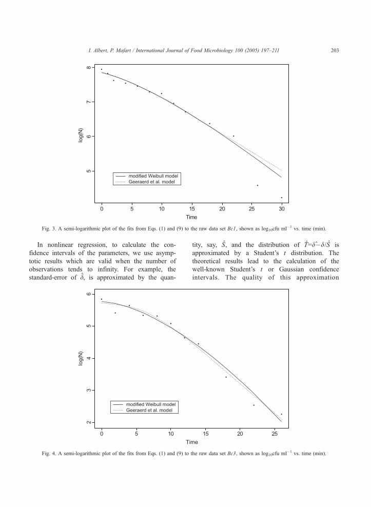
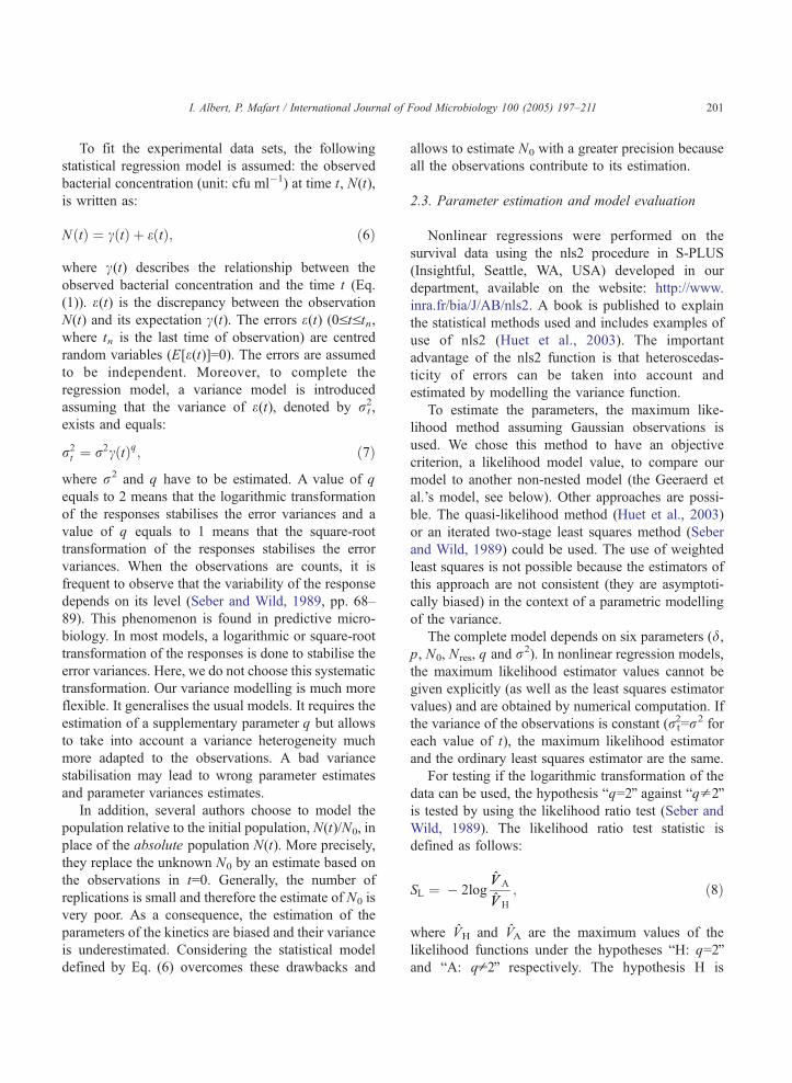
Fig. 3. A semi-logarithmic plot of the fits from Eqs. (1) and (9) to the raw data set Bc1, shown as log10cfu ml�1 vs. time (min).


In nonlinear regression, to calculate the con-

fidence intervals of the parameters, we use asymp-

totic results which are valid when the number of

observations tends to infinity. For example, the

standard-error of d, is approximated by the quan-

Fig. 4. A semi-logarithmic plot of the fits from Eqs. (1) and (9) to

tity, say, S, and the distribution of T=d�d/S is

approximated by a Student’s t distribution. The

theoretical results lead to the calculation of the

well-known Student’s t or Gaussian confidence

intervals. The quality of this approximation

the raw data set Bc3, shown as log10cfu ml�1 vs. time (min).

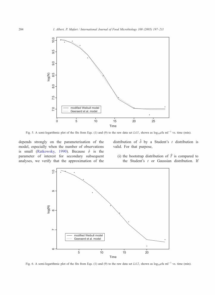
Fig. 5. A semi-logarithmic plot of the fits from Eqs. (1) and (9) to the raw data set Li11, shown as log10cfu ml�1 vs. time (min).


depends strongly on the parameterisation of the

model, especially when the number of observations

is small (Ratkowsky, 1990). Because d is the

parameter of interest for secondary subsequent

analyses, we verify that the approximation of the

Fig. 6. A semi-logarithmic plot of the fits from Eqs. (1) and (9) to t

distribution of d by a Student’s t distribution is

valid. For that purpose,

(i) the bootstrap distribution of T is compared to

the Student’s t or Gaussian distribution. If

he raw data set Li12, shown as log10cfu ml�1 vs. time (min).

Fig. 7. A semi-logarithmic plot of the fit from Eq. (1) to the raw data set Cb4, shown as log10cfu ml�1 vs. time (min) (at t=48 min, the two

points are superposed).


these two distributions are close, the approx-

imation of the distribution of T by a Student’s

t or Gaussian distribution is valid (Huet et al.,

2003).

Fig. 8. A semi-logarithmic plot of the fit from Eq. (1) to the raw data set C

points are superposed).

(ii) The confidence ellipsoids (obtained under

hypotheses of a Gaussian distribution for each

parameter) and the likelihood contours (based on

the likelihood ratio test and independent of the

b5, shown as log10cfu ml�1 vs. time (min) (at t=0.85 min, the two

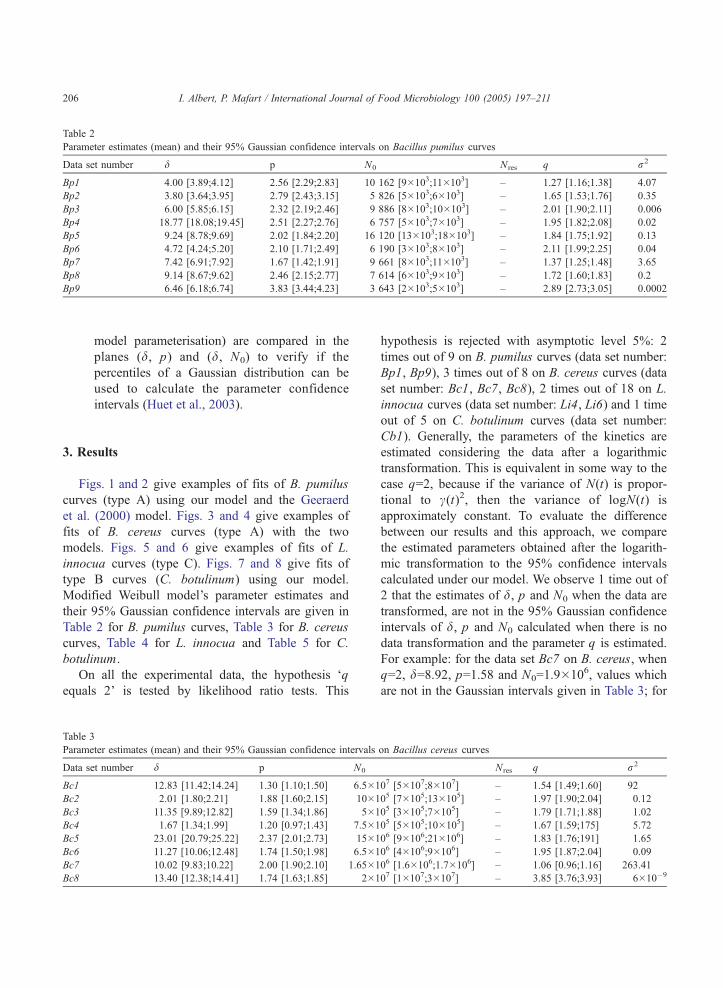
Table 2

Parameter estimates (mean) and their 95% Gaussian confidence intervals on Bacillus pumilus curves

Data set number d p N0 Nres q r2

Bp1 4.00 [3.89;4.12] 2.56 [2.29;2.83] 10 162 [9�103;11�103] – 1.27 [1.16;1.38] 4.07

Bp2 3.80 [3.64;3.95] 2.79 [2.43;3.15] 5 826 [5�103;6�103] – 1.65 [1.53;1.76] 0.35

Bp3 6.00 [5.85;6.15] 2.32 [2.19;2.46] 9 886 [8�103;10�103] – 2.01 [1.90;2.11] 0.006

Bp4 18.77 [18.08;19.45] 2.51 [2.27;2.76] 6 757 [5�103;7�103] – 1.95 [1.82;2.08] 0.02

Bp5 9.24 [8.78;9.69] 2.02 [1.84;2.20] 16 120 [13�103;18�103] – 1.84 [1.75;1.92] 0.13

Bp6 4.72 [4.24;5.20] 2.10 [1.71;2.49] 6 190 [3�103;8�103] – 2.11 [1.99;2.25] 0.04

Bp7 7.42 [6.91;7.92] 1.67 [1.42;1.91] 9 661 [8�103;11�103] – 1.37 [1.25;1.48] 3.65

Bp8 9.14 [8.67;9.62] 2.46 [2.15;2.77] 7 614 [6�103;9�103] – 1.72 [1.60;1.83] 0.2

Bp9 6.46 [6.18;6.74] 3.83 [3.44;4.23] 3 643 [2�103;5�103] – 2.89 [2.73;3.05] 0.0002


model parameterisation) are compared in the

planes (d, p) and (d, N0) to verify if the

percentiles of a Gaussian distribution can be

used to calculate the parameter confidence

intervals (Huet et al., 2003).

3. Results

Figs. 1 and 2 give examples of fits of B. pumilus

curves (type A) using our model and the Geeraerd

et al. (2000) model. Figs. 3 and 4 give examples of

fits of B. cereus curves (type A) with the two

models. Figs. 5 and 6 give examples of fits of L.

innocua curves (type C). Figs. 7 and 8 give fits of

type B curves (C. botulinum) using our model.

Modified Weibull model’s parameter estimates and

their 95% Gaussian confidence intervals are given in

Table 2 for B. pumilus curves, Table 3 for B. cereus

curves, Table 4 for L. innocua and Table 5 for C.

botulinum.

On all the experimental data, the hypothesis dqequals 2T is tested by likelihood ratio tests. This

Table 3

Parameter estimates (mean) and their 95% Gaussian confidence intervals

Data set number d p N0

Bc1 12.83 [11.42;14.24] 1.30 [1.10;1.50] 6.5�1

Bc2 2.01 [1.80;2.21] 1.88 [1.60;2.15] 10�1

Bc3 11.35 [9.89;12.82] 1.59 [1.34;1.86] 5�1

Bc4 1.67 [1.34;1.99] 1.20 [0.97;1.43] 7.5�1

Bc5 23.01 [20.79;25.22] 2.37 [2.01;2.73] 15�1

Bc6 11.27 [10.06;12.48] 1.74 [1.50;1.98] 6.5�1

Bc7 10.02 [9.83;10.22] 2.00 [1.90;2.10] 1.65�1

Bc8 13.40 [12.38;14.41] 1.74 [1.63;1.85] 2�1

hypothesis is rejected with asymptotic level 5%: 2

times out of 9 on B. pumilus curves (data set number:

Bp1, Bp9), 3 times out of 8 on B. cereus curves (data

set number: Bc1, Bc7, Bc8), 2 times out of 18 on L.

innocua curves (data set number: Li4, Li6) and 1 time

out of 5 on C. botulinum curves (data set number:

Cb1). Generally, the parameters of the kinetics are

estimated considering the data after a logarithmic

transformation. This is equivalent in some way to the

case q=2, because if the variance of N(t) is propor-

tional to c(t)2, then the variance of logN(t) is

approximately constant. To evaluate the difference

between our results and this approach, we compare

the estimated parameters obtained after the logarith-

mic transformation to the 95% confidence intervals

calculated under our model. We observe 1 time out of

2 that the estimates of d, p and N0 when the data are

transformed, are not in the 95% Gaussian confidence

intervals of d, p and N0 calculated when there is no

data transformation and the parameter q is estimated.

For example: for the data set Bc7 on B. cereus, when

q=2, d=8.92, p=1.58 and N0=1.9�106, values which

are not in the Gaussian intervals given in Table 3; for

on Bacillus cereus curves

Nres q r2

07 [5�107;8�107] – 1.54 [1.49;1.60] 92

05 [7�105;13�105] – 1.97 [1.90;2.04] 0.12

05 [3�105;7�105] – 1.79 [1.71;1.88] 1.02

05 [5�105;10�105] – 1.67 [1.59;175] 5.72

06 [9�106;21�106] – 1.83 [1.76;191] 1.65

06 [4�106;9�106] – 1.95 [1.87;2.04] 0.09

06 [1.6�106;1.7�106] – 1.06 [0.96;1.16] 263.41

07 [1�107;3�107] – 3.85 [3.76;3.93] 6�10�9

Table 4

Parameter estimates (mean) and their 95% Gaussian confidence intervals on Listeria innocua curves

Data set

number

d p N0 Nres q r2

Li1 11.85 [10.17;13.52] 1.42 [1.23;1.6] 11�109 [6�109;16�109] 521 822 [4�105;6�105] 2.33 [2.28;2.38] 10�3

Li2 12.60 [11.44;13.76] 2.12 [1.65;2.59] 7.5�109 [5�109;8�109] 672 286 [6�103;13�105] 1.62 [1.57;1.66] 201

Li3 12.55 [11.43;13.66] 1.93 [1.62;2.23] 6.5�109 [5�109;8�109] 554 237 [1�105;9�105] 1.77 [1.74;1.83] 5.2

Li4 11.94 [10.89;12.98] 1.84 [1.55;2.13] 7.5�109 [6�109;9�109] 344 068 [�3�104;71�104]* 1.59 [1.55;1.64] 304

Li5 5.7 [5.17;6.24] 2.27 [1.96;2.58] 6.5�109 [4�109;9�109] 2 559 [6�102;44�102] 1.87 [1.82;1.93] 1.45

Li6 11.59 [10.52;12.67] 3.76 [2.79;4.72] 3�1010 [1�109;5�109] 13 315 826 [12�106;14�106] 2.64 [2.58;2.69] 10�6

Li7 5.02 [4.69;5.35] 2.81 [2.42;3.19] 4.5�1010 [3�1010;6�1010] 4 178 450 [3�106;5�106] 2.09 [2.05;2.15] 10�3

Li8 9.68 [8.77;10.59] 2.05 [1.65;2.46] 11�109 [8�109;14�109] 10 238 430 [7�106;13�106] 1.89 [1.85;1.94] 0.39

Li9 8.51 [7.23;9.78] 1.68 [1.3;2.05] 12�109 [7�109;17�109] 2 308 624 [8�105;37�105] 1.88 [1.83;1.93] 1.00

Li10 6.88 [5.93;7.84] 1.61 [1.38;1.84] 17�109 [9�109;25�109] 897 123 [7�105;10�105] 2.27 [2.22;2.33] 10�4

Li11 7.52 [6.54;8.5] 2.43 [1.94;2.91] 7�109 [2�109;12�109] 155 389 [12�104;18�104] 2.22 [2.16;2.28] 10�3

Li12 7.86 [6.41;9.26] 1.59 [1.26;1.91] 13.5�109 [6�109;21�109] 154 103 [6�104;24�104] 2.02 [1.97;2.07] 0.09

Li13 6.55 [5.53;7.58] 1.58 [1.29;188] 10.5�109 [6�109;15�109] 74 549 [8�103;141�103] 1.79 [1.74;1.85] 6.61

Li14 4.02 [3.11;4.92] 1.26 [1.07;1.45] 16�109 [4�109;28�109] 1 835 [9�102;27�102] 2.00 [1.95;2.07] 0.12

Li15 6 [5.52;6.59] 1.46 [1.28;1.65] 8.5�109 [7�109;10�109] 99 986 [�2�104;22�104]* 1.63 [1.59;1.68] 383

Li16 4.71 [4.27;5.15] 1.49 [1.35;1.63] 8.5�109 [6�109;11�109] 30 555 [9�103;5�104] 2.04 [1.99;2.09] 0.02

Li17 2.74 [2.37;3.1] 1.74 [1.51;1.97] 9�109 [4�109;14�109] 6 354 [4�103;8�103] 2.07 [2.01;2.14] 0.03

Li18 5.41 [4.65;6.18] 1.42 [1.25;1.58] 11�109 [6�109;16�109] 1 145 [�3�103;5�103]* 2.14 [2.08;2.19] 10�3

* According to the Gaussian confidence interval, in these cases, Nres can be considered to be equal to 0 (equivalent to a Wald test).


the data set Bc8, the behaviour is similar: d=11.07,p=1.48 and N0=4.9�107 when q=2.

Table 6 gives the AIC criterion value of each

model for type A and C curves. The AIC values are

smallest for the modified Weibull model on 5 curves

on 9 for B. pumilus, on 6 curves on 8 for B. cereus

and on 8 curves on 18 for L. innocua. According to

this criterion, the modified Weibull model is pref-

erable for these curves (when it is the smallest). In

fact, the observed values of the criterion are often very

close between the two models which shows that the

two model fits are equivalent on these two types of

curves. This result can be also confirmed by the

visualisation of the two model fits on the experimental

data (see Figs. 1–6). Often the curves are very close.

The shoulder effect might be more marked with the

Geeraerd et al. model. But the model proposed by

Table 5

Parameter estimates (mean) and their 95% Gaussian confidence intervals

Data set number d p N0

Cb1 3.43 [2.08;4.79] 0.42 [0.35;0.49] 725 203

Cb2 2.17 [0.8;3.53] 0.43 [0.36;0.49] 521 412

Cb3 0.84 [0.51;1.18] 0.39 [0.35;0.45] 461 642

Cb4 0.26 [0.21;3.13] 0.44 [0.41;0.46] 534 042

Cb5 0.04 [0.02;0.06] 0.32 [0.29;0.35] 644 579

Geeraerd et al. does not allow to fit upward concavity

curves (type B) as ours.

On the experimental data, the parameterisation of

the model is evaluated. Note that in nonlinear models,

the model parameterisation is an important point

because it can cause curvature effects (local minima

can appear) and problems of parameter identifiability

(for example, we could have difficulties to estimate

the d parameter if it is too close to zero). We need to

assess the parametric nonlinearity of the model.

Particularly, the parameter of interest d is studied. A

weak parametric nonlinearity of this parameter will

allow to calculate the confidence intervals of the

parameter from the Normal or Student’s t percentiles.

From each data set, the bootstrap distribution of

T=d�d/S is calculated from 1000 bootstrap simula-

tions. It can be done with nls2. For example, Fig. 9

on Clostridium botulinum curves

Nres q r2

185 [58�107;86�107] – 1.64 [1.59;1.69] 29.38

535 [10�107;93�107] – 2.5 [2.44;2.56] 10�3

995 [34�107;57�107] – 1.8 [1.74;1.86] 1.77

387 [41�107;64�107] – 1.95 [1.89;2.01] 0.07

341 [47�107;81�107] – 1.89 [1.83;1.95] 0.33

Table 6

AIC criterion values (the minimum value between the two models is

in bold type)

Data set

number

Modified Weibull

model’s AIC

Geeraerd et al.

model’s AIC

Bacillus pumilus

Bp1 169.66 168.44

Bp2 166.01 163.48

Bp3 175.65 179.45

Bp4 121.99 124.45

Bp5 270.38 275.45

Bp6 179.03 176.43

Bp7 175.72 178.10

Bp8 155.15 146.79

Bp9 153.44 167.64

Bacillus cereus

Bc1 421.96 422.99

Bc2 291.53 290.91

Bc3 249.21 247.08

Bc4 169.66 275.85

Bc5 280.41 286.43

Bc6 196.58 203.52

Bc7 139.95 146.28

Bc8 214.10 229.88

Listeria innocua

Li1 495.67 493.86

Li2 455.06 453.81

Li3 480.14 480.95

Li4 525.07 524.47

Li5 357.72 361.92

Li6 485.16 484.85

Li7 338.22 344.02

Li8 406.52 402.86

Li9 407.69 405.71

Li10 352.05 343.42

Li11 364.67 365.25

Li12 402.10 396.79

Li13 383.90 367.70

Li14 342.97 333.91

Li15 422.70 424.25

Li16 372.97 373.74

Li17 324.91 329.38

Li18 385.03 389.79


gives the histogram of this distribution on the data set

Bp1 with superposed Normal and Student’s t centred

and scaled distributions. We observe that the distri-

butions are very close. The 95% bootstrap confidence

interval of d, IB (IB=[d�b1�a/2S;d�ba/2S] where ba

is the 95 percentile of the bootstrap distribution of T),

equals to [3.84;4.18], compared to the Gaussian:

[3.89;4.12] and to the Student’s t confidence interval:

[3.84;4.17]. They are almost similar. Moreover, the

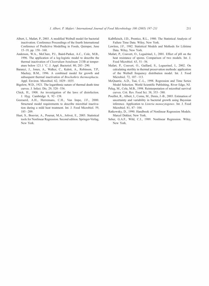
likelihood contours (based on the likelihood ratio test

and independent of the model parameterisation) and

the confidence ellipses (assuming Normal distribu-

tions) of d among the p and N0 parameters (Figs. 10

and 11, respectively, for the data set Bp1) are similar.

The likelihood contours are close to the ellipses. This

result indicates a weak parametric nonlinearity of the

d parameter. The 95% confidence interval of d based

on the likelihood contours equals to [3.86;4.12]. Same

results are found on all the experimental data. So, the

specific parameterisation of the Peleg and Cole’s

model with d ¼ 1k

� �1=pis satisfactory. The confidence

intervals of the d parameter calculated from the

Normal or Student’s t percentiles are acceptable and

very close to the intervals based on the likelihood

contours.

4. Discussion

We have demonstrated the capacities of our

model to model a large range of inactivation curves:

curves with or without shoulder, with or without

tailing. A good fit of the inactivation curve is

essential to obtain good estimates of the model

parameters. It is an important point for the

bsecondaryQ modelling which uses the bprimaryQparameter estimates. The goodness-of-fit of the

bprimaryQ modelling guarantees that the parameter

values are a good summary of the bprimaryQmodelling. An accurate fit is essential to obtain

reliable predictions (for example, reliable decontami-

nation times). Before the fits, we verified using the

sensitivity functions (Huet et al., 2003) if the

experimental designs (the chosen time values) permit

an accurate estimation of all the model parameters.

Those functions are a first approach to deal with

this. The results (not shown here) are often

conclusive. Perhaps, some reserves can be done

concerning the Nres parameter which could be better

evaluated with longer times of observation.

On the experimental data curves A and C fits, our

model fits are similar globally to the fits produced by

the model of Geeraerd et al. (2000). Moreover, our

model is more flexible because it permits curve B fits.

Note that we have sometimes encountered difficulties

to estimate the Geeraerd et al. model (difficulties to fix

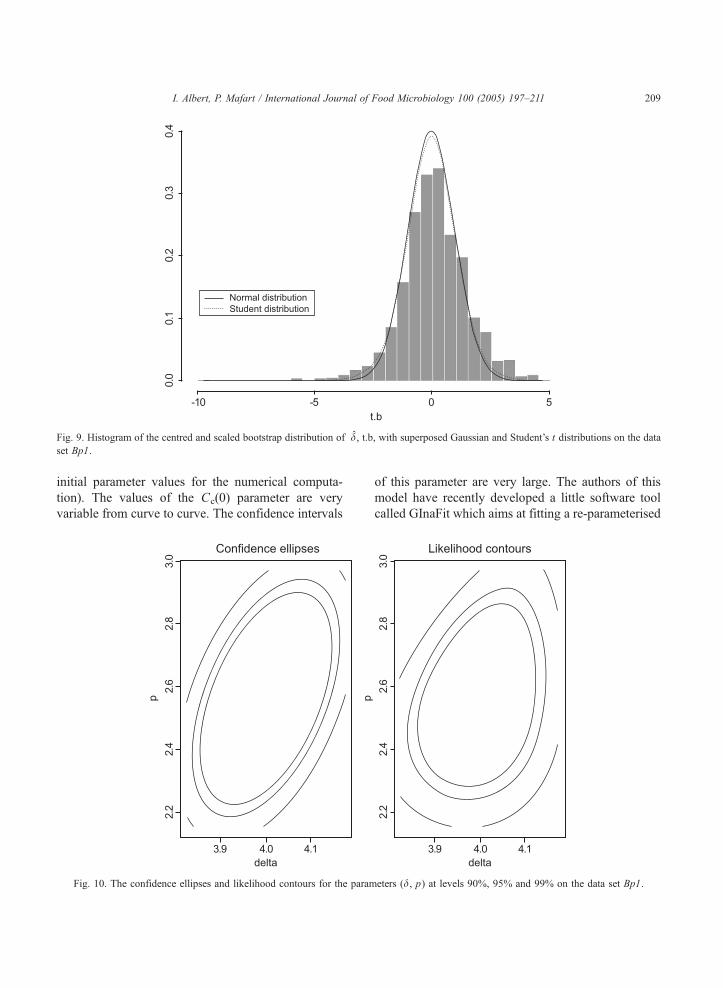
Fig. 9. Histogram of the centred and scaled bootstrap distribution of d, t.b, with superposed Gaussian and Student’s t distributions on the data

set Bp1.


initial parameter values for the numerical computa-

tion). The values of the Cc(0) parameter are very

variable from curve to curve. The confidence intervals

Fig. 10. The confidence ellipses and likelihood contours for the param

of this parameter are very large. The authors of this

model have recently developed a little software tool

called GInaFit which aims at fitting a re-parameterised

eters (d, p) at levels 90%, 95% and 99% on the data set Bp1.

Fig. 11. The confidence ellipses and likelihood contours for the parameters (d, N0) at levels 90%, 95% and 99% on the data set Bp1.


version of their model on inactivation data. The tool

can be downloaded at http://www.kuleuven.ac.be/cit/

biotec/index.htm. In addition, the book of Ratkowsky

(1990) gives indications for good parameterisations of

nonlinear models.

The parameterisation of the model we propose

seems to be satisfactory for the d parameter. For the q

and p parameters, no estimation difficulty has been

encountered. We can only note that the Gaussian

confidence intervals for the q parameter are a little bit

narrower compared to the likelihood ratio test (often

they did not contain the 2 value whereas the

hypothesis q=2 is not rejected by the likelihood ratio

test). Confidence intervals based on the likelihood

contours will be in accordance with the test. For the p

parameter, we tested by likelihood ratio tests if it can

be considered constant by strain. For the four types of

bacteria strains studied, the hypothesis is rejected.

More investigations concerning this scope have to be

done. It should be interesting to study the behaviour

of p according to environmental factors (temperature,

pH, aw, possibly other factors and possibly their

interactions).

The parameterisation proposed here is very inter-

esting because it introduces a d parameter close to the

D value established for sterilisation processes. D is

yet a starting point of bsecondaryQ modelling (Bige-

low, 1921) and d (when estimating without Nres) has

been modelled according to environmental factors

(Mafart et al., 2001). An important work has to be

done in this domain, especially to find the better

function linking the d value to the environmental

factors. In failure time data analysis, authors have

introduced covariates directly in the Weibull model.

This possibility has to be studied. The direct

introduction of covariates in the bprimaryQ model

would avoid a two-stage estimation which is embar-

rassing for parameter estimation because the response

of the bsecondaryQ model, for example the dparameter, is not an observation but an estimation

(from the bprimaryQ modelling). In addition, a

Bayesian approach allows a single-step evaluation

(Pouillot et al., 2003).

References

Akaike, H., 1973. Information theory and an extension of the

maximum likelihood principle. In: Petrov, B.N., Czaki, F.

(Eds.), Second International Symposium on Information Theory.

Akademiai Kiado, pp. 267–281.

http://www.kuleuven.ac.be/cit/biotec/index.htm


Albert, I., Mafart, P., 2003. A modified Weibull model for bacterial

inactivation. Conference Proceedings of the fourth International

Conference of Predictive Modelling in Foods, Quimper, June

15–19, pp. 158–160.

Anderson, W.A., McClure, P.J., Baird-Parker, A.C., Cole, M.B.,

1996. The application of a log-logistic model to describe the

thermal inactivation of Clostridium botulinum 213B at temper-

ature below 121.1 8C. J. Appl. Bacteriol. 80, 283–290.Baranyi, J., Jones, A., Walker, C., Kaloti, A., Robinson, T.P.,

Mackey, B.M., 1996. A combined model for growth and

subsequent thermal inactivation of Brochothrix thermosphacta.

Appl. Environ. Microbiol. 62, 1029–1035.

Bigelow, W.D., 1921. The logarithmic nature of thermal death time

curves. J. Infect. Dis. 29, 528–536.

Chick, H., 1908. An investigation of the laws of disinfection.

J. Hyg. Cambridge 8, 92–158.

Geeraerd, A.H., Herremans, C.H., Van Impe, J.F., 2000.

Structural model requirements to describe microbial inactiva-

tion during a mild heat treatment. Int. J. Food Microbiol. 59,

185–209.

Huet, S., Bouvier, A., Poursat, M.A., Jolivet, E., 2003. Statistical

tools for Nonlinear Regression. Second edition. Springer-Verlag,

New York.

Kalbfleisch, J.D., Prentice, R.L., 1980. The Statistical Analysis of

Failure Time Data. Wiley, New York.

Lawless, J.F., 1982. Statistical Models and Methods for Lifetime

Data. Wiley, New York.

Mafart, P., Couvert, O., Leguerinel, I., 2001. Effect of pH on the

heat resistance of spores. Comparison of two models. Int. J.

Food Microbiol. 63, 51–56.

Mafart, P., Couvert, O., Gaillard, S., Leguerinel, I., 2002. On

calculating sterility in thermal preservation methods: application

of the Weibull frequency distribution model. Int. J. Food

Microbiol. 72, 107–113.

McQuarrie, A.D., Tsai, C.-L., 1998. Regression and Time Series

Model Selection. World Scientific Publishing, River Edge, NJ.

Peleg, M., Cole, M.B., 1998. Reinterpretation of microbial survival

curves. Crit. Rev. Food Sci. 38, 353–380.

Pouillot, R., Albert, I., Cornu, M., Denis, J.-B., 2003. Estimation of

uncertainty and variability in bacterial growth using Bayesian

inference. Application to Listeria monocytogenes. Int. J. Food

Microbiol. 81, 87–104.

Ratkowsky, D., 1990. Handbook of Nonlinear Regression Models.

Marcel Dekker, New York.

Seber, G.A.F., Wild, C.J., 1989. Nonlinear Regression. Wiley,

New York.

A modified Weibull model for bacterial inactivation

Documents

Transcript of A modified Weibull model for bacterial inactivation