A New Weibull-Pareto Distribution: Properties and Applications

M. H. TAHIR1, GAUSS M. CORDEIRO2, AYMAN ALZAATREH3, M.MANSOOR4 AND M. ZUBAIR5

1Department of Statistics, The Islamia University of Bahawalpur, PakistanEmail: mtahir.stat@gmail.com

2Department of Statistics, Federal University of Pernambuco, Recife, PE, Brazil3Department of Mathematics and Statistics, Austin Peay State University, USA

4Department of Statistics, Punjab College, Model-Town A, Bahawalpur, Pakistan5Department of Statistics, Government Degree College Kahrorpacca, Pakistan

Abstract. Many distributions have been used as lifetime models. Recently, a generator of dis-tributions called the Weibull-G class was proposed by Bourguignon et al. (2014). We propose anew three-parameter Weibull-Pareto distribution, which can produce the most important hazardrate shapes, namely constant, increasing, decreasing, bathtub and upsidedown-bathtub. Variousstructural properties of the new distribution are derived including explicit expressions for the mo-ments and incomplete moments, Bonferroni and Lorenz curves, mean deviations, mean residuallife, mean waiting time and generating and quantile functions. The Renyi and q entropies are alsoderived. We obtain the density function of the order statistics and their moments. The model pa-rameters are estimated by maximum likelihood and the observed information matrix is determined.The usefulness of the new model is illustrated by means of two real data sets on Wheaton riverflood and bladder cancer. In the two applications, the new model provides better fits than theKumaraswamy-Pareto, beta-exponentiated Pareto, beta-Pareto, exponentiated-Pareto and Paretomodels.

Keywords: Hazard function; Likelihood estimation; Moment; Pareto distribution; Weibull-G class

Mathematics Subject Classification (2010) 60E05; 62F10; 62N05

1. Introduction

The Pareto distribution was pioneered by Vilfraddo Pareto (1896) to explore unequal distributionof wealth and income. It is widely used in modeling actuarial data (e.g. insurance risk) because ofits heavy tail properties. It has also wider applications in hydrology, telecommunications, povertymeasurement, migration, size of cities and firms, word frequencies, business mortality, service timein queuing theory, etc.

A random variable T has the Pareto distribution with two parameters α > 0 and θ > 0, if its

1

cumulative distribution function (cdf) is given by

Hα,θ(x) = 1−(x

θ

)−α, x > θ. (1)

Then, its probability density function (pdf) reduces to

hα,θ(x) =(α

x

) (x

θ

)−α, x > θ > 0, α > 0. (2)

Keeping in view of its applications, various authors have extended the Pareto distribution to exploreproperties and for efficient estimation of its parameters. The first parameter induction to the Paretomodel called the generalized Pareto (GP) distribution was pioneered by Pickands (1975). Stoppa(1990) proposed another three-parameter generalization of the Pareto distribution known as theexponentiated Pareto (“EP” for short) distribution. It is also named the Stoppa distribution. Thethree-parameter EP cdf is given by

Gα,θ,λ(x) ={

1−(x

θ

)−α}λ

, x > θ > 0, α, λ > 0. (3)

The density function corresponding to (3) becomes

gα,θ,λ(x) = λ(α

x

) (x

θ

)−α{

1−(x

θ

)−α}λ−1

, x > θ > 0, α, λ > 0. (4)

Gupta et al. (1998) discussed the EP distribution using the Lehmann alternative type I (due toLehmann, 1953) by taking the λth power of the baseline cdf G(x), say G(x)λ. Akinsete et al. (2008)extended the Pareto distribution by adding two extra shape parameters based on the beta-G classof distributions pioneered by Eugene et al. (2002). The four-parameter beta-Pareto (BP) cdf isgiven by

F (x; a, b, α, θ) =1

B(a, b)

∫ Hα,θ(x)

0wa−1 (1− w)b−1 dw = IHα,θ(x)(a, b), x > θ, a, b, α > 0, (5)

where Hα,θ(x) = 1− (x/θ)−α is given by (1), Iw(a, b) is the incomplete beta function ratio, and a

and b are two additional shape parameters whose role is to govern the skewness and tail weights.The beta-EP (BEP) distribution was defined by Nassar and Nada (2011), Zea et al. (2012)

and Mansoor (2013) by using the beta-G class (Eugene et al., 2002) of distributions. So, thefive-parameter BEP cdf becomes

F (x; a, b, α, θ, λ) = IGα,θ,λ(x)(a, b), x > θ, a, b, α, λ > 0, (6)

where Gα,θ,λ(x) is given by equation (3).Further, Mahmoudi (2011) defined the beta generalized Pareto (BGP) distribution and studied

some useful properties for modeling extreme value data. Alzaatreh (2012) used the Transformed-Transformer (T-X) family of distributions (Alzaatreh et al., 2011, 2013b) to define the gamma-Pareto (GaP) cdf by

F (x; a, b, θ) =∫ W (G(x))

0π(x) dx, (7)

2

where W (G(x)) = − log[1−G(x)] and π(x) = xa−1 e−x/b/[Γ(a) ba], a, b > 0.

Based on the T-X family, Alzaatreh et al. (2013a) defined the Weibull-Pareto-T-X (WPTX)distribution. If a random variable Z has the Weibull distribution with parameters α and β, thenthe WPTX cumulative function is given by

F (x; α, β, θ) = 1− e−[β log(xθ )]α , x > θ > 0 α, β > 0. (8)

Bourguignon et al. (2013) defined the Kumaraswamy-Pareto (KwP) from the Kummaraswamy-G (Kw-G) class of distributions proposed by Cordeiro and de Castro (2011). The four-parameterKwP cdf is given by

F (x; a, b, α, θ) = 1−[1−

{1−

(x

θ

)−α}a ]b

, x > θ > 0, a, b, α > 0. (9)

Zagrafos and Balakrishnan (2009) pioneered a versatile and flexible gamma-G class of distri-butions based on Stacy’s generalized gamma distribution and record value theory. More recently,Bourguignon et al. (2014) proposed the Weibull-G class of distributions influenced by the Zografos-Balakrishnan-G class. Let G(x; Θ) and g(x; Θ) denote the cumulative and density functions of abaseline model with parameter vector Θ and consider the Weibull cdf πW (x) = 1− e−xb

(for x > 0)with scale parameter one and shape parameter b > 0. Bourguignon et al. (2014) replaced theargument x by G(x; Θ)/G(x; Θ), where G(x; Θ) = 1−G(x; Θ), and defined the cdf of their class ofdistributions, say Weibull-G(b, Θ), by

F (x; b, Θ) = b

∫ hG(x;Θ)

G(x;Θ)

i

0xb−1 e−xb

dx = 1− e−h

G(x;Θ)

G(x;Θ)

ib, x ∈ <, b > 0. (10)

Then, the Weibull-G class pdf is given by

f(x; b, Θ) = b g(x; Θ)[G(x; Θ)b−1

G(x; Θ)b+1

]e−h

G(x;Θ)

G(x;Θ)

ib, x ∈ <, b > 0. (11)

It is noteworthy to mention that (10) is a special case of the T-X family proposed by Alzaatreh etal. (2013b) in (7) by taking W (G(x)) = G(x; Θ)/G(x; Θ) and π(x) as the Weibull cdf.

In this context, we propose an extension of the Pareto model called the Weibull-Pareto (“WP”for short) distribution based on equations (10) and (11). The proposed distribution is more flexiblethan the WPTX (Alzaatreh et al., 2013a) model. For example, the hazard function shapes of theWP distribution can be constant, increasing, decreasing, bathtub and upside down bathtub. Alza-atreh et al. (2013a) noted a significant problem to estimate the parameters of the their distributionusing maximum likelihood. Further, they showed that the maximum likelihood estimates (MLEs)have considerable bias values. On the other hand, the MLEs of the WP parameters have lower biasvalues (see Table 1).

The paper is outlined as follows. In Section 2, we define the WP distribution and discussthe shapes of the density and hazard rate functions. We provide a mixture representation for itsdensity function in Section 3. Structural properties such as the ordinary and incomplete moments,Bonferroni and Lorenz curves, mean deviations, mean residual life, mean waiting time, generating

3

and quantile functions are derived in Section 4. In Section 5, we determine the Renyi and q

entropies. The density of the order statistics is investigated in Section 6. The maximum likelihoodestimation of the model parameters is discussed in Section 7. We explore the usefulness of thenew model by means of two real data sets in Section 8. Finally, Section 9 offers some concludingremarks.

2. The WP Distribution

Inserting (1) in equation (10), the three-parameter WP cdf is defined by

F (x) = F (x; b, α, θ) = 1− e−[(xθ )α−1]b , x > θ > 0. (12)

The pdf corresponding to (12) becomes

f(x) = f(x; b, α, θ) =b α

θαxα−1

[(x

θ

)α− 1

]b−1e−[(x

θ )α−1]b , x > θ > 0. (13)

Henceforth, a random variable X with density function (13) is denoted by X ∼WP(b, α, θ). Thesurvival function (sf) (S(t)), hazard rate function (hrf) (h(t)), reversed-hazard rate function (rhrf)(r(t)) and cumulative hazard rate function (chrf) (H(t)) of X are given by

S(x) = e−[(xθ )α−1]b , x > θ,

h(x) =bα

θαxα−1

[(x

θ

)α− 1

]b−1, x > θ, (14)

r(x) =b

(αx

) (xθ

)α [(xθ

)α − 1]b−1 e−[(x

θ )α−1]b

1− e−[(xθ )α−1]b

, x > θ,

andH(x) =

[(x

θ

)α− 1

]b, x > θ,

respectively.

Lemma 1 provides some relations of the WP distribution with the well-known Weibull andexponential distributions.

Lemma 1 (Transformation): (a) If a random variable Y follows the Weibull distribution withshape parameter b and scale parameter one, then the random variable X = θ (Y + 1)1/α follows theWP (b, α, θ) distribution.

(b) If a random variable Y follows the exponential distribution, then the random variable X =θ(Y 1/b + 1

)1/αfollows the WP (b, α, θ) distribution.

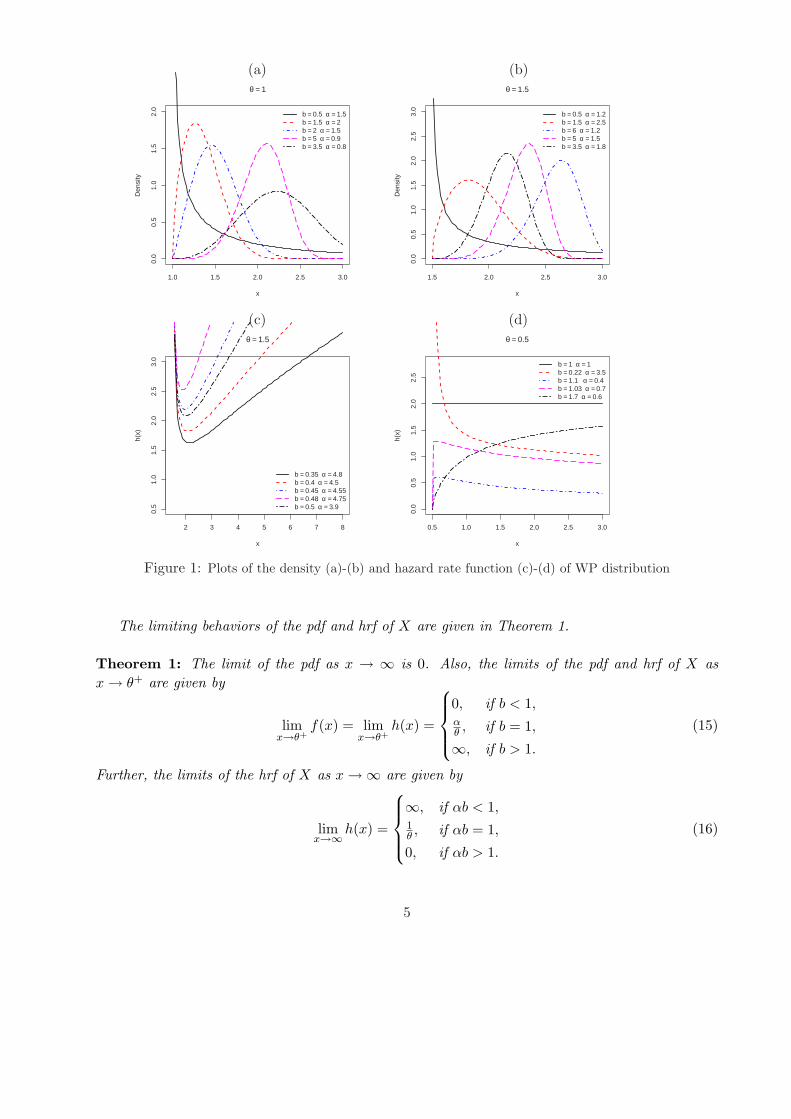
Plots of the WP density and hazard rate functions for some parameter values are displayed inFigures 1 and 2, respectively.

4

(a) (b)

1.0 1.5 2.0 2.5 3.0

0.0

0.5

1.0

1.5

2.0

θ = 1

x

Den

sity

b = 0.5 α = 1.5b = 1.5 α = 2b = 2 α = 1.5b = 5 α = 0.9b = 3.5 α = 0.8

1.5 2.0 2.5 3.0

0.0

0.5

1.0

1.5

2.0

2.5

3.0

θ = 1.5

x

Den

sity

b = 0.5 α = 1.2b = 1.5 α = 2.5b = 6 α = 1.2b = 5 α = 1.5b = 3.5 α = 1.8

(c) (d)

2 3 4 5 6 7 8

0.5

1.0

1.5

2.0

2.5

3.0

θ = 1.5

x

h(x)

b = 0.35 α = 4.8b = 0.4 α = 4.5b = 0.45 α = 4.55b = 0.48 α = 4.75b = 0.5 α = 3.9

0.5 1.0 1.5 2.0 2.5 3.0

0.0

0.5

1.0

1.5

2.0

2.5

θ = 0.5

x

h(x)

b = 1 α = 1b = 0.22 α = 3.5b = 1.1 α = 0.4b = 1.03 α = 0.7b = 1.7 α = 0.6

Figure 1: Plots of the density (a)-(b) and hazard rate function (c)-(d) of WP distribution

The limiting behaviors of the pdf and hrf of X are given in Theorem 1.

Theorem 1: The limit of the pdf as x → ∞ is 0. Also, the limits of the pdf and hrf of X asx → θ+ are given by

limx→θ+

f(x) = limx→θ+

h(x) =

0, if b < 1,αθ , if b = 1,

∞, if b > 1.

(15)

Further, the limits of the hrf of X as x →∞ are given by

limx→∞h(x) =

∞, if αb < 1,1θ , if αb = 1,

0, if αb > 1.

(16)

5

Proof: Most results of this type can be easily shown from equations (13) and (14). We only needto obtain the result in (15). To do this, one can see from the hrf in (14) that

limx→∞h(x) =

bα

θ

{lim

x→∞

(x

θ

)αb−1b−1

[1−

(x

θ

)−α]}b−1

=bα

θlim

x→∞

(x

θ

)αb−1

This implies the result in (16).

2.1. Shapes of the density and hazard rate functions

We provide two theorems for the shapes of the density and hazard rate functions.

Theorem 2: The WP distribution is unimodal and has a unique mode at x = x0. When b ≤ 1,the mode is x0 = θ and when b > 1, the mode at x0 is the solution of k(x) = 0, where

k(x) =(x

θ

)α{

αb− αb[(x

θ

)α− 1

]b+1− 1

}− α + 1. (17)

Proof: The derivative with respect to x of equation (13) can be reduced to

d f(x)dx

= α b θα xα−2[(x

θ

)α− 1

]b−2e−[(x/θ)α−1]b k(x). (18)

From (18), the critical point of f(x) are x = θ and x = x0, where k(x0) = 0. Case I: if b ≤ 1, itis easy to show from (13) that f(x) is a decreasing function, and then f(x) has a unique mode atx = θ. Case II: if b > 1, Theorem 1 indicates that limx→θ+ f(x) = 0, which implies that x = θ cannot be a mode point. Therefore, the modes of f(x) are the solutions of k(x) = 0. Finally, we needto show that k(x) = 0 has one solution. One can easily see that k′(x) < 0 whenever b > 1. Hence,k(x) = 0 has at most one solution. Using the facts from Theorem 1 that limx→θ+ f(x) = 0 andlimx→∞ f(x) = 0, we conclude that f(x) must have a unique mode.

Theorem 3: The hrf of X possesses the following shapes:(i) Constant failure rate (CFR) whenever α = b = 1,(ii) Increasing failure rate (IFR) whenever αb ≥ 1 and b > 1,(iii) Decreasing failure rate (DFR) whenever αb ≤ 1 and b < 1,(iv) Upsidedown bathtub rate (UBT) whenever αb ≤ 1, b > 1 and α < 1,(v) Bathtub rate (BT) whenever αb ≥ 1, b < 1 and α > 1.

Proof: Based on equation (14), the hrf of X can be expressed as

h(x) = α b θ−1

{(x

θ

)αb−1b−1

[1−

(x

θ

)−α]}b−1

, x > θ,

which implies (i), (ii) and (iii). Now, the derivative of h(x) in (15) is given by

h′(x) = α b θ−2(x

θ

)α−1 [(x

θ

)α− 1

]b−2w(x),

6

where w(x) = (αb− 1)(

xθ

)α − (α− 1).

The critical value of h(x) is at x0 = θ(

α−1αb−1

)1/α, which is defined only when α(b − 1) > 0.

Now, if αb ≤ 1, b > 1 and α < 1, then x0 is defined and w(x) > 0 for all x > x0 and w(x) < 0 forall θ < x < x0. This proves (iv). Similar argument can be used to prove (v).

3. Mixture Representation

In order to obtain a simplified form for the WP pdf, we expand (13) in power series. Then, theWP pdf can be expressed as

f(x; b, α, θ) = b g(x)G(x)b−1

G(x)b+1e−h

G(x)

G(x)

ib. (19)

Inserting (1) and (2) in equation (19), we obtain

f(x; b, α, θ) = b(α

x

) (x

θ

)−α

[1− (

xθ

)−α]b−1

[1−

{1− (

xθ

)−α}]b+1

× e−24

{1−(x

θ )−α}

1−{

1−(xθ )−α

}35

b

︸ ︷︷ ︸A

.

Consider the quantity A in the last equation. After a power series expansion, it reduces to

A =∞∑

k=0

(−1)k

k!

[1− (

xθ

)−α]bk

[1−

{1− (

xθ

)−α}]bk

.

Combining the last two results, we have

f(x; b, α, θ) = b(α

x

) (x

θ

)−α∞∑

k=0

(−1)k

k!

[1−

(x

θ

)−α]b(k+1)−1 [

1−{

1−(x

θ

)−α}]−[b(k+1)+1]

︸ ︷︷ ︸B

.

Consider the quantity B in the last equation. After a power series expansion, we obtain

B =∞∑

j=0

Γ(b(k + 1) + j + 1)Γ(b(k + 1) + 1) j!

[1−

(x

θ

)−α]j

.

Combining the last two results, we can write

f(x; b, α, θ) =∞∑

k,j=0

(−1)k

k! j!b Γ(b(k + 1) + j + 1)

(bk + b + j)Γ(b(k + 1) + 1)︸ ︷︷ ︸vk,j

× [b(k + 1) + j](α

x

) (x

θ

)−α[1−

(x

θ

)−α]bk+b+j−1

︸ ︷︷ ︸gα,θ,b(k+1)+j(x)

7

In a more simplified form, the last equation reduces to

f(x; b, α, θ) =∞∑

k,j=0

vk,j gα,θ,b(k+1)+j(x). (20)

Equation (20) reveals that the WP density function can be expressed as a mixture of EP den-sities. So, several of its mathematical properties can be derived from those of the EP distribution.Equation (20) is the main result of this section.

4. Some Structural Properties

4.1Moments

The rth moment of X follows from (20) as

µ′r = E(Xr) =∞∑

k,j=0

vk,j

∫ ∞

θxr gα,θ,b(k+1)+j(x) dx

and then (for r ≤ α)

µ′r = θr∞∑

k,j=0

vk,j [b(k + 1) + j] B(1− r

α , b[k + 1] + j), (21)

where B(a, b) =∫ 10 wa−1(1− w)b−1dw is the beta function.

In particular, setting r = 1 in (21), the mean of X reduces to

µ′1 = θ

∞∑

k,j=0

vk,j [b(k + 1) + j] B(1− 1

α , b[k + 1] + j).

Further, the central moments (µn) and cumulants (κn) of X are easily obtained from (21) as

µn =n∑

k=0

(n

k

)(−1)k µ′k1 µ′n−k and κn = µ′n −

n−1∑

k=1

(n− 1k − 1

)κk µ′n−k,

respectively, where κ1 = µ′1. Thus, κ2 = µ′2 − µ′21 , κ3 = µ′3 − 3µ′2µ′1 + 2µ′31 , etc. The skewness and

kurtosis measures can be calculated from the ordinary moments using well-known relationships.The nth descending factorial moment of X (for n = 1, 2, . . .) is

µ′(n) = E[X(n)] = E[X(X − 1)× · · · × (X − n + 1)] =n∑

j=0

s(n, j) µ′j ,

where s(n, j) = (j!)−1 [djj(n)/dxj ]x=0 is the Stirling number of the first kind.

4.2 Incomplete Moments

8

Let Y be a random variable having the EP distribution with parameters α, θ and λ. Then, the rthincomplete moment of Y (for r < α) is given by

mr,Y (z) =∫ z

θyr gα,θ,λ(y) dy = λ θrBz

(1− r

α , λ),

where Bx(a, b) =∫ x0 wa−1 (1− w)b−1dw is the incomplete beta function.

The rth incomplete moment of X follows from (20) (for r < α) as

mr,X(z) =∫ z

θxr gα,θ,b(k+1)+j(x) dx = θr

∞∑

k,j=0

vk,j [b(k + 1) + j] Bz

(1− r

α , b[k + 1] + j). (22)

The main application of the first incomplete moment is related to the Bonferroni and Lorenzcurves. These curves are very useful in several fields such economics, reliability, demography, insu-rance and medicine. For a given probability π, they are defined by BX(π) = m1,X(q)/(π µ′1) andLX(π) = m1,X(q)/µ′1, respectively, where m1,X(q) comes from (22) with r = 1 and q = QX(π) isdetermined from (24) (given in Section 4.4).

Another important application of the first incomplete moment refers to the mean deviationsabout the mean and the median defined by δ1 =

∫∞0 |x − µ| f(x)dx and δ2 =

∫∞0 |x −M | f(x)dx,

respectively, where µ′1 = E(X) denotes the mean and M = θ{1 + [− log(0.5)]1/b

}1/αdenotes the

median, respectively. These measures can be determined from the expressions δ1 = 2µ′1F (µ′1) −2m1,X(µ′1) and δ2 = µ′1 − 2m1,X(M), where F (µ′1) is given by (12) and m1,X(·) is calculated from(22).

A third application of the first incomplete moment is to obtain the mean residual life and themean waiting time. The mean residual life and the mean waiting time are defined by m(t; b, α, θ) =1/S(t) [1−m1,X(t)]− t and µ(t; b, α, θ) = t− [m1,X(t)/F (t; b, α, θ)], where S(t) = 1− F (t) comesfrom (12).

4.3 Generating Function

First, we obtain the moment generating function (mgf) of the EP distribution, say Mα,θ,λ(t). Byexpanding the binomial term in (4), we can write

Mα,θ,λ(t) = α λ∞∑

m=0

(−1)m θ(m+1)α

(λ− 1

m

) ∫ ∞

θx−(m+1)α−1 et xdx.

The last integral can be computed using Maple. For t ≤ 0 and p > 0 and q > 0, let J(q, p, t) =∫∞q x−p et x dx. We can obtain using this software

J(q, p, t) = (−t)p q

[−π csc(p π)

t q Γ(p)− p Γ(−p)

q t+

etq

(−t)p+1 qp+1+

p Γ(−p,−t q)t q

],

where Γ(λ, x) =∫∞x wλ−1 e−wdw is the complementary incomplete gamma function. Thus,

Mα,θ,λ(t) = α λ∞∑

m=0

(−1)m θ(m+1)α

(λ− 1

m

)J(θ, [m + 1]α + 1, t).

9

Combining (20) and the last result, it follows the mgf of X as

M(t) =∞∑

m=0

pm J(θ, [m + 1]α + 1, t), (23)

where pm = (−1)m α θ(m+1)α∑∞

k,j=0 [b(k+1)+j] vk,j

(b(k+1)+j−1

m

). Equation (23) is the main result

of this section.

4.4Quantile Function and Simulation

By inverting (12), the quantile function (qf) of X follows as

QX(u) = F−1(u) = θ{

1 + [− log(1− u)]1/b}1/α

. (24)

Simulating WP random variable is straightforward. Let U be the uniform variate on the unitinterval (0, 1]. Thus, using the inverse transformation method, the random variable

X = θ{

1 + [− log(1− U)]1/b}1/α

,

has pdf given by (13), i.e., X ∼WP(b, α, θ).

5. Renyi and q-Entropies

The entropy of a random variable is a measure of the uncertainty variation. The Renyi entropy ofX is defined as

IR(δ) =1

1− δlog [I(δ)]

where I(δ) =∫< f δ(x) dx, δ > 0 and δ 6= 1.

Now, consider

f δ(x; b, α, θ)] = bδ g(x)δ G(x)δ(b−1)

G(x)δ(b+1)e−δh

G(x)

G(x)

ib.

Using a power series for the exponential function and the generalized binomial expansion in theabove result, we obtain

f δ(x; b, α, θ) =∞∑

k,j=0

sk,j gδ(x) G(x)kb+δ(b−1)+j , (25)

where

sk,j =(−1)k δk

bδk! j!Γ(kb + δ[b + 1] + j)

Γ(kb + δ[b + 1]).

Next, inserting (2) and (1) in (25), and then integrating

I(δ) =∞∑

k,j=0

sk,j (αθ)δ

∫ ∞

θ

[(x

θ

)−α] δ(α+1)

α[1−

(x

θ

)−α]kb+δ(b−1)+j

dx

10

For δ(α + 1) > 1 and δ(b − 1) > −1, transforming variables and integrating, the last equationbecomes

I(δ) =∞∑

k,j=0

sk,j (αθ)δ (θ/α) B(δ(α + 1)− 1

α, kb + δ(b− 1) + j + 1

). (26)

Hence, the Renyi entropy reduces to

IR(δ) =1

1− δlog

∞∑

k,j=0

sk,j (αθ)δ (θ/α) B(δ(α + 1)− 1

α, kb + δ(b− 1) + j + 1

) .

The q-entropy, say Hq(f), is defined by

Hq(f) =1

q − 1log [1− Iq(f)] ,

where Iq(f) =∫< f q(x) dx, q > 0 and q 6= 1. From equation (26), we can easily obtain (for

δ(α + 1) > 1 and q(b− 1) > −1)

Hq(f) =1

q − 1log

1−

∞∑

k,j=0

s?k,j (αθ)q (θ/α) B

(q(α + 1)− 1α

, kb + q(b− 1) + j + 1) ,

where s?k,j = (−1)k δk bδ Γ(kb + q[b + 1] + j)/[k! j!Γ(kb + q[b + 1])].

6. Order Statistics

Here, we give the density of the ith order statistic Xi:n, fi:n(x) say, in a random sample of size n

from the WP distribution. It is well known that (for i = 1, . . . , n)

fi:n(x) =1

B(i, n− i + 1)f(x)F i−1(x) {1− F (x)}n−i.

Using the binomial expansion, we can rewrite fi:n(x) as

fi:n(x) =f(x)

B(i, n− i + 1)

n−i∑

j=0

(−1)j(n−i

j

)F (x)i+j−1. (27)

Further, we have

F (x)i+j−1 =∞∑

k=0

(−1)k(i+j−1

k

)exp

[−(k + 1)

{(x

θ

)α− 1

}b]

and then by inserting (13) in (27), we obtain

fi:n(x) =∞∑

k=0

tk+1 f(x; b, α, θ), (28)

11

where

tk+1 =1

(k + 1)B(i, n− i + 1)

n−i∑

j=0

(−1)j+k

(n− i

j

)(i + j − 1

k

)

and

f(x; b, α, θ) =b α (k + 1)

θαxα−1

[(x

θ

)α− 1

]b−1exp

{−(k + 1)

[(x

θ

)α− 1

]b}

is the WP density function with parameters b, α and θ. So, the density function of the WP orderstatistics is a mixture of WP densities. Based on equation (28), we can obtain some structuralproperties of the WP order statistics from those of the WP properties.

7. Estimation and Information Matrix

Here, we discuss maximum likelihood estimation and inference for the WP distribution. Letx1, . . . , xn be a sample from X ∼WP(b, α, θ) and let Θ = (b, α, θ)> be the vector of the modelparameters with known θ (since x > θ). The likelihood function for Θ reduces to

` = `(Θ) = n log(bα)− n α log(θ) + (α− 1)n∑

i=1

log(xi) + (b− 1)n∑

i=1

log(zi)−n∑

i=1

(zbi ). (29)

Since θ is assumed known, the score vector can be denoted by U(Θ) = (∂`/∂b, ∂`/∂α)>, wherethe components corresponding to the model parameters are determined by differentiating (29). Bysetting zi = [(xi/θ)α − 1], we obtain

∂`

∂b=

n

b+

n∑

i=1

log zi −n∑

i=1

zbi log zi

∂`

∂α=

n

α+

1α

n∑

i=1

log(1 + zi) +b− 1

α

n∑

i=1

[(1 + zi) log(1 + zi)

zi

]− b

α

n∑

i=1

zb−1i (1 + zi) log (1 + zi).

The maximum likelihood estimates (MLEs) of the model parameters are the solution of the nonlin-ear equations U(Θ) = 0, which can be solved iteratively. The elements of the observed informationmatrix Jn(Θ) = {Jrs} (for r, s = b, α) are given by

Jbb = − n

b2−

n∑

i=1

[zbi (log zi)2

],

Jαα = − n

α2− b− 1

α2

n∑

i=1

[(1 + zi) [log(1 + zi)]2

z2i

]

− b

α

n∑

i=1

[(1 + zi) [log(1 + zi)]2

{zb−1i + (b− 1) zb−2

i (1 + zi)}]

,

12

Jb α =1α

n∑

i=1

[(1 + zi) log(1 + zi)

zi

]− b

α

n∑

i=1

[zb−1i (1 + zi) (log zi) {log (1 + zi)}

]

− 1α

n∑

i=1

[zb−1i (1 + zi) log (1 + zi)

].

The distribution of√

n(Θ −Θ) can be approximated by the multivariate normal N2(0,J(Θ)−1)distribution, where J(Θ) = limn→∞ n−1Jn(Θ) is the unit information matrix. The estimatedasymptotic multivariate normal N2(0, Jn(Θ)−1) distribution of Θ can be used to construct ap-proximate confidence intervals for the model parameters. The 100(1− γ)% confidence intervals for

b and α are given by b±zγ/2×√

var(b) and α±zγ/2×√

var(α), respectively, where the var(·)’s are

the diagonal elements of Jn(Θ)−1 corresponding to the model parameters, and zγ/2 is the quantile(1− γ/2) of the standard normal distribution.

7.1. Simulation study

We evaluate the performance of the maximum likelihood method for estimating the WP parametersusing Monte Carlo simulation for a total of sixteen parameter combinations and the process isrepeated 200 times. Two different sample sizes n = 100 and 300 are considered. The MLEs andthe standard deviations of the parameter estimates are listed in Table 1. In this simulation study,we assume θ to be unknown and estimate it by the minimum order statistic x(1). The MLEs of α

and b are determined by solving the nonlinear equations U(Θ) = 0, where xi 6= x(1). From Table1, we note that the ML method performs well for estimating the model parameters. Also, as thesample size increases, the biases and the standard deviations of the MLEs decrease as expected.

Table 1: MLEs and standard deviations for various parameter values

Sample size Actual values Estimated values Standard deviations

n b α θ b α θ b α θ

100 0.5 0.5 1 0.5045 0.5138 1.0004 0.0560 0.0434 0.0011

0.5 0.5 2 0.5077 0.5092 2.0007 0.0624 0.0422 0.0019

0.5 0.8 1 0.5078 0.7915 1.0066 0.0429 0.0658 0.0098

0.5 0.8 2 0.5139 0.7877 2.0145 0.0456 0.0656 0.0179

0.5 1 1 0.5204 0.9612 1.0203 0.0344 0.0824 0.0200

0.5 1 2 0.5180 0.9570 2.0419 0.0367 0.0803 0.0432

0.5 2 1 0.5877 1.6137 1.1886 0.0492 0.1606 0.1006

0.5 2 2 0.5918 1.6003 2.3880 0.0490 0.1670 0.1992

0.8 0.5 1 0.7794 0.5312 1.0003 0.0884 0.0459 0.0008

0.8 0.5 2 0.7931 0.5216 2.0005 0.0910 0.0449 0.0008

0.8 0.8 1 0.8190 0.8074 1.0049 0.0713 0.0683 0.0060

13

Table 1 (Continued)

Sample size Actual values Estimated values Standard deviations

n b α θ b α θ b α θ

100 0.8 0.8 2 0.8313 0.7838 2.0097 0.0759 0.0689 0.0146

0.8 1 1 0.8309 0.9603 1.0129 0.0538 0.0785 0.0136

0.8 1 2 0.8334 0.9591 2.0246 0.0582 0.0747 0.0244

0.8 2 1 0.9472 1.6120 1.1159 0.0843 0.1672 0.0623

0.8 2 2 0.9566 1.5758 2.2380 0.0861 0.1647 0.1273

1 0.5 1 0.9761 0.5295 1.0002 0.1115 0.0421 0.0004

1 0.5 2 0.9870 0.5155 2.0003 0.1168 0.0420 0.0006

1 0.8 1 1.0094 0.8031 1.0042 0.0907 0.0702 0.0055

1 0.8 2 1.0258 0.7868 2.0075 0.0895 0.0603 0.0088

1 1 1 1.0344 0.9834 1.0109 0.0796 0.0805 0.0112

1 1 2 1.0453 0.9587 2.0207 0.0770 0.0870 0.0191

1 2 1 1.1725 1.6353 1.0840 0.0932 0.1658 0.0440

1 2 2 1.1862 1.6028 2.1834 0.1088 0.1694 0.0991

2 0.5 1 1.9345 0.5404 1.0001 0.2125 0.0421 0.0002

2 0.5 2 1.9570 0.5293 2.0002 0.2021 0.0414 0.0004

2 0.8 1 2.0227 0.8127 1.0017 0.1624 0.0636 0.0020

2 0.8 2 2.0287 0.7984 2.0034 0.1741 0.0653 0.0045

2 1 1 2.0497 0.9725 1.0050 0.1395 0.0777 0.0048

2 1 2 2.0667 0.9781 2.0095 0.1511 0.0831 0.0099

2 2 1 2.3585 1.6277 1.0443 0.2108 0.1712 0.0234

2 2 2 2.3629 1.6008 2.0909 0.1908 0.1625 0.0466

300 0.5 0.5 1 0.4932 0.5140 1.0000 0.0350 0.0262 0.0001

0.5 0.5 2 0.4931 0.5133 2.0001 0.0310 0.0274 0.0002

0.5 0.8 1 0.4991 0.8109 1.002 0.0256 0.0405 0.0023

0.5 0.8 2 0.5042 0.8029 2.0040 0.0263 0.0412 0.0057

0.5 1 1 0.5064 0.9890 1.0059 0.0199 0.0470 0.0059

0.5 1 2 0.5070 0.9806 2.0138 0.0225 0.0462 0.0134

0.5 2 1 0.5490 1.7775 1.1146 0.0269 0.1244 0.0600

0.5 2 2 0.5500 1.7700 2.2181 0.0280 0.1238 0.1172

0.8 0.5 1 0.7794 0.5253 1.0000 0.0510 0.0230 0.0001

0.8 0.5 2 0.7822 0.5173 2.0000 0.0521 0.0263 0.0001

14

Table 1 (Continued)

Sample size Actual values Estimated values Standard deviations

n b α θ b α θ b α θ

300 0.8 0.8 1 0.8028 0.8027 1.0013 0.0412 0.0385 0.0017

0.8 0.8 2 0.8043 0.8038 2.0025 0.0451 0.0431 0.0029

0.8 1 1 0.8087 0.9935 1.0046 0.0315 0.0485 0.0048

0.8 1 2 0.8086 0.9878 2.0082 0.0313 0.0479 0.0092

0.8 2 1 0.8742 1.7872 1.0632 0.0427 0.1150 0.0329

0.8 2 2 0.8722 1.7899 2.1240 0.0441 0.1155 0.0735

1 0.5 1 0.9686 0.5261 1.0000 0.0587 0.0261 0.0001

1 0.5 2 0.9772 0.5172 2.0001 0.0594 0.0245 0.0001

1 0.8 1 0.9974 0.8094 1.0009 0.0469 0.0410 0.0011

1 0.8 2 1.0090 0.7961 2.0022 0.0485 0.0401 0.0028

1 1 1 1.0092 0.9953 1.0036 0.0414 0.0483 0.0035

1 1 2 1.0108 0.9880 2.0063 0.0397 0.0464 0.0061

1 2 1 1.0837 1.8013 1.0485 0.0472 0.1220 0.0235

1 2 2 1.0952 1.7731 2.1040 0.0536 0.1187 0.0529

2 0.5 1 1.9069 0.5385 1.0000 0.1249 0.0245 0.0001

2 0.5 2 1.9389 0.5228 2.0000 0.1159 0.0252 0.0001

2 0.8 1 1.9919 0.8116 1.0004 0.0929 0.0386 0.0006

2 0.8 2 1.9891 0.8078 2.0008 0.0951 0.0406 0.0011

2 1 1 2.0136 0.9989 1.0019 0.0834 0.0471 0.0020

2 1 2 2.0132 0.9897 2.0034 0.0815 0.0442 0.0040

2 2 1 2.1655 1.8139 1.0245 0.1056 0.1251 0.0130

2 2 2 2.1779 1.7910 2.0497 0.1049 0.1095 0.0276

8. Applications

In this section, we illustrate the usefulness of the WP distribution. We fit this distribution to twodata sets and compare the results with the KwP, BEP, BP, EP and Pareto distributions.

8.1 Wheaton River Data

The data consist to the 72 exceedances for the years 1958–1984 (rounded to one decimal place) offlood peaks (in m3/s) of the Wheaton River near Carcross in Yukon Territory, Canada. The dataare listed in Table 1. Choulakian and Stephens (2001), Akinsete et al. (2008), Mahmoudi (2011)and Bourguignon et al. (2013) analyzed the these data using the BP, BGP and KwP distributions.

15

Table 2: Exceedances of Wheaton River flood data

1.7 2.2 14.4 1.1 0.4 20.6 5.3 0.7 1.9 13.0 12.0 9.31.4 18.7 8.5 25.5 11.6 14.1 22.1 1.1 2.5 14.4 1.7 37.60.6 2.2 39.0 0.3 15.0 11.0 7.3 22.9 1.7 0.1 1.1 0.69.0 1.7 7.0 20.1 0.4 2.8 14.1 9.9 10.4 10.7 30.0 3.65.6 30.8 13.3 4.2 25.5 3.4 11.9 21.5 27.6 36.4 2.7 64.01.5 2.5 27.4 1.0 27.1 20.2 16.8 5.3 9.7 27.5 2.5 27.0

8.2 Bladder Cancer Data

We consider an uncensored data set corresponding to the remission times (in months) of a randomsample of 128 bladder cancer patients. Bladder cancer is a disease in which abnormal cells multiplywithout control in the bladder. The most common type of bladder cancer recapitulates the normalhistology of the urothelium and is known as transitional cell carcinoma. These data were previouslystudied by Lemonte (2012), Zea et al. (2012), Lee and Wang (2003) and Lemonte and Cordeiro(2013). Table 3 lists the remission times of the bladder cancer.

Table 3: The remission times of the bladder cancer

0.08 0.20 0.40 0.50 0.51 0.81 0.90 1.05 1.19 1.26 1.35 1.40 1.461.76 2.02 2.02 2.07 2.09 2.23 2.26 2.46 2.54 2.62 2.64 2.69 2.692.75 2.83 2.87 3.02 3.25 3.31 3.36 3.36 3.48 3.52 3.57 3.64 3.703.82 3.88 4.18 4.23 4.26 4.33 4.34 4.40 4.50 4.51 4.87 4.98 5.065.09 5.17 5.32 5.32 5.34 5.41 5.41 5.49 5.62 5.71 5.85 6.25 6.546.76 6.93 6.94 6.97 7.09 7.26 7.28 7.32 7.39 7.59 7.62 7.63 7.667.87 7.93 8.26 8.37 8.53 8.65 8.66 9.02 9.22 9.47 9.74 10.06 10.3410.66 10.75 11.25 11.64 11.79 11.98 12.02 12.03 12.07 12.63 13.11 13.29 13.8014.24 14.76 14.77 14.83 15.96 16.62 17.12 17.14 17.36 18.10 19.13 20.28 21.7322.69 23.63 25.74 25.82 26.31 32.15 34.26 36.66 43.01 46.12 79.05

We estimate the model parameters of the distributions by the method of maximum like-lihood. There exists many maximization methods in R Packages like NR (Newton-Raphson),BFGS (Broyden-Fletcher-Goldfarb-Shanno), BHHH (Berndt-Hall-Hall-Hausman), SANN (Simul-ated-Annealing), NM (Nelder-Mead) and L-BFGS-B. Here, the MLEs are computed using Limited-Memory quasi-Newton code for Bound-constrained optimization (L-BFGS-B) and the measures ofgoodness of fit including the Akaike information criterion (AIC), consistent Akaike information cri-terion (CAIC), Bayesian information criterion (BIC), Hannan-Quinn information criterion (HQIC),Anderson-Darling (A∗) and Cramer–von Mises (W ∗) are computed to compare the fitted models.The statistics W ∗ and A∗ are described in details in Chen and Balakrishnan (1995). In general, thesmaller the values of these statistics, the better the fit to the data. The required computations arecarried out using a script AdequacyModel of the R-package written by Pedro Rafael Diniz Marinho,Cicero Rafael Barros Dias and Marcelo Bourguignon. It is freely available fromhttp://cran.r-project.org/web/packages/AdequacyModel/AdequacyModel.pdf.

16

Tables 4 and 6 list the MLEs and their corresponding standard errors (in parentheses) of themodel parameters. The model selection is carried out using the following statistics:

AIC = −2 ˆ+ 2p, CAIC = −2 ˆ+2pn

n− p− 1,

BIC = −2 ˆ+ p log(n), and HQIC = 2 log{log(n)

[k − 2 ˆ] }

,

where ˆ denotes the log-likelihood function evaluated at the MLEs, p is the number of parameters,and n is the sample size. The statistics AIC, CAIC, BIC, HQIC, W ∗ and A∗ are listed in Tables 5and 7.

Table 4: MLEs and their standard errors (in parentheses) for Wheaton river flood data

Distribution a b α λ θ

WP - 4.4363 0.0987 - 0.1000- (0.4409) (0.0020) - -

BEP 0.1742 83.7393 0.3562 83.8231 0.1000(0.0632) (251.1542) (0.0926) (26.3243) -

KwP 11.2069 31.9168 0.1910 - 0.1000(3.0323) (31.2434) (0.06356) - -

BP 22.2915 12.7688 0.1602 - 0.1000(4.4687) (12.1744) (0.1085) - -

EP - - 0.7197 62.4789 0.1000- - (0.0628) (21.4784) -

Pareto - - 0.1548 - 0.1000- - (0.0184) - -

Table 5: The statistics ˆ, AIC, CAIC , BIC , HQIC, A∗ and W ∗ for Wheaton river flood data

Distribution ˆ AIC CAIC BIC HQIC A∗ W ∗

WP -249.3965 502.7930 502.9695 507.3184 504.5926 0.9819 0.1746BEP -248.0554 504.1107 504.7168 513.1615 507.7099 1.0320 0.1903KwP -252.4078 510.8157 511.1739 517.6037 513.515 1.4604 0.2619BP -255.8893 517.7787 518.1369 524.5667 520.4781 1.9532 0.3445EP -260.9832 525.9665 526.1429 530.4918 527.7661 2.5498 0.4410Pareto -335.2348 672.4695 672.5275 674.7322 673.3693 1.9146 0.3381

17

Table 6: MLEs and their standard errors (in parentheses) for bladder cancer data

Distribution a b α λ θ

WP - 3.5707 0.1466 - 0.08- (0.2477) (0.0027) - -

KwP 7.1911 66.0736 0.1756 - 0.08(1.2078) (67.9676) (0.0616) - -

BEP 0.5457 30.3072 0.2952 14.3993 0.08(0.3509) (16.9047) (0.1112) (10.6635) -

BP 14.9920 23.6299 0.1158 - 0.08(1.9701) (44.0328) (0.1770) - -

EP - - 0.8513 23.9408 0.08- - (0.0546) (4.7808) -

Pareto - - 0.2319 - 0.08- - (0.0206) - -

Table 7: The statistics ˆ, AIC, CAIC, BIC , HQIC, A∗ and W ∗ for bladder cancer data

Distribution ˆ AIC CAIC BIC HQIC A∗ W ∗

WP -407.4665 818.9331 819.0298 824.6214 821.2442 0.3650 0.0563KwP -409.2100 824.4200 824.6151 832.9525 827.8866 0.5351 0.0770BEP -409.0659 826.1318 826.4596 837.5085 830.7540 0.5061 0.0725BP -418.9310 843.8620 844.0571 852.3946 847.3287 1.8946 0.2930EP -432.0897 868.1794 868.2762 873.8678 870.4905 3.6418 0.5865Pareto -539.5911 1081.1820 1081.2140 1084.0260 1082.3380 1.8785 0.2904

In Tables 5 and 7, the WP model is compared with the KwP, BEP, BP and EP models. Wenote that the WP model has the lowest values of the AIC, BIC, CAIC, HQIC, A∗ and W ∗ statisticsamong all fitted models. So, the WP distribution could be chosen as the best model for both datasets. The histogram of the data and plots of the estimated pdf and cdf of the WP model aredisplayed in Figure 2. It is clear that the new distribution provides a better fit to the histogramand therefore could be chosen as the best model for both data sets.

9. Concluding Remarks

In this paper, we propose a three-parameter Weibull-Pareto (WP) distribution based on theWeibull-G family of distributions recently introduced by Bourguignon et al. (2014). We derivesome of its structural properties and provide explicit expressions for the ordinary and incompletemoments, mean residual life, mean waiting time, generating function, mode and quantile function.We also obtain expressions for the Renyi entropy, q entropy and the density of ith order statistic.The model parameters are estimated by the method of maximum likelihood. The usefulness of thenew model is illustrated by means of two real life data sets. The new model provides consistently abetter fit than other competitive lifetime models. We hope that the new model will attract widerapplications in several areas such as engineering, survival data, economics (income inequality) andothers.

18

(a) Estimated pdfs (data set 1) (b) Estimated cdfs (data set 1)

x

pdf

0 20 40 60 80

0.00

0.01

0.02

0.03

0.04

0.05

0.06

0.07

WPBEPBPKwPEP

0 20 40 60 80

0.0

0.2

0.4

0.6

0.8

1.0

x

cdf

WPBEPBPKwPEP

(c) Estimated pdfs (data set 2) (d) Estimated cdfs (data set 2)

x

pdf

0 10 20 30 40 50 60 70

0.00

0.01

0.02

0.03

0.04

0.05

WPBEPBPKwPEP

0 20 40 60

0.0

0.2

0.4

0.6

0.8

1.0

x

cdf

WPBEPBPKwPEP

Figure 2: Plots of the fitted WP, BEP, BP, KwP and EP distributions

Acknowledgments

The authors would like to thank the Editor-in-Chief, and the referee for constructive commentswhich greatly improved the paper.

References

Akinsete, A., Famoye, F., Lee, C. (2008). The beta-Pareto distribution. Statistics 42: 547–563.

Alzaatreh, A. (2011). A New Method for Generating Families of Continuous Distributions. Ph.D.thesis, Central Michigan University, Mount Pleasant: Michigan.

Alzaatreh, A., Famoye, F., Lee, C. (2012). Gamma-Pareto distribution and its applications. Jour-nal of Modern Applied Statistical Methods 11:78–94.

Alzaatreh, A., Famoye, F., Lee, C. (2013a). Weibull-Pareto distribution and its applications.Communications in Statistics–Theory and Methods 42:1673–1691.

19

Alzaatreh, A., Famoye, F., Lee, C. (2013b). A new method for generating families of continuousdistributions. Metron 71:63–79.

Bourguignon, M., Silva, M.B., Zea, L.M., Cordeiro, G.M. (2013). The Kumaraswamy Paretodistribution. Journal of Statistical Theory and Applications 12:129–144.

Bourguignon, M., Silva, R.B., Cordeiro, G.M. (2014). The Weibull–G family of probability distri-butions. Journal of Data Science 12:53–68.

Chen, G., Balakrishnan, N. (1995). A general purpose approximate goodness-of-fit test. Journalof Quality Technology 27:154–161.

Choulakian, V., Stephens, M.A. (2001). Goodness-of-fit for the generalized Pareto distribution.Technometrics 43:478–484.

Cordeiro, G.M., de Castro, M. (2011). A new family of generalized distributions. Journal ofStatistical Computation and Simulation 81:883–893.

Eugene, N., Lee, C., Famoye, F. (2002). Beta-normal distribution and its applications. Communi-cations in Statistics–Theory and Methods 31:497–512.

Gupta, R.C., Gupta, P.I., Gupta, R.D. (1998). Modeling failure time data by Lehmann alternatives.Communications in Statistics–Theory and Methods 27:887–904.

Lee, E.T., Wang, J.W. (2003). Statistical Methods for Survival Data Analysis, 3rd edition, Wiley:New York.

Lehmann, E.E. (1953). The power of rank tests. Annals of Mathematical Statistics 24:23–43.

Lemonte, A.J. (2012). The beta log-logistic distribution. To appear in Brazilian Journal of Prob-ability and Statistics.

Lemonte, A.J., Cordeiro, G.M. (2013). An extended Lomax distribution. Statistics 47:800–816.

Mahmoudi, E. (2011). The beta generalized Pareto distribution with application to lifetime data.Mathematics and Computers in Simulation 81:2414–2430.

Mansoor, M. (2013). Properties and Extensions of Stoppa Income Size Distribution. UnpublishedM.Phil. thesis, Department of Statistics, The Islamia University of Bahawalpur: Pakistan.

Nassar, M.M., Nada, N.K. (2011). The beta generalized Pareto distribution. Journal of Statistics:Advances in Theory and Applications 6:1–17.

Pareto, V. (1896). La courbe de la rpartition de la richesse. In Recueil publi par la Facult de Droitl.occasion de l.exposition nationale suisse (Eds) C. ViretGenton, Lausanne: Universit de Lausanne,pp. 373–387.

Pickands, J. (1975). Statistical inference using extreme order statistics. Annals of Statistics 3:119–131.

20

Stoppa, G. (1990). A new model for income size distribution. In: C. Dagum and M. Zenga (eds.)Income and Wealth Distribution, Inequality and Poverty, Springer, New York, pp. 33–41.

Zea, L.M., Silva, R.B., Bourguignon, M., Santos, A.M., Cordeiro, G.M. (2012). The beta exponen-tiated Pareto distribution with application to bladder cancer susceptibility. International Journalof Statistics and Probability 1:8–19.

Zografos, K., Balakrishnan, N. (2009). On families of beta- and generalized gamma-generateddistributions and associated inference. Statistical Methodology 6:344–362.

21