Double Weighted Weibull Distribution Properties and ... - IISTE's

Mathematical Theory and Modeling www.iiste.org

ISSN 2224-5804 (Paper) ISSN 2225-0522 (Online)

Vol.6, No.7, 2016

28

Double Weighted Weibull Distribution Properties and Application

Aamir Saghir, Muhammad Saleem

Department of Mathematics, Mirpur University of Science and Technology

(MUST), Mirpur AJK.

This paper offering a new weighted distribution known as the Double Weighted

Weibull Distribution (DWWD). The statistical properties of the (DWWD) are derived

and discussed, including the mean, variance, coefficient of variation, moments, mode,

reliability function, hazard function and the reverse hazard function. Also the

parameters of this distribution are estimated by the maximum likelihood estimation

method. The plots of survival function, hazard function and reverse hazard function of

(DWWD) are also presented. The worth of the distribution has been demonstrated by

applying it to real life data.

Keywords:Weighted distribution, Double Weighted distribution, Weibull

distribution, Reliability estimation.

1. Introduction

In the literature the Weibull distribution attract the most of the researchers due to its

wide range applications. Different generalization of the Weibull distribution are available in

the literature as Merovci and Elbatal (2015) developed the Weibull-Rayleigh distribution and

demonstrated its application using lifetime data. Almalki and Yuan (2013) presented the new

modified Weibull distribution by combining the Weibull and the modified Weibull

distribution in a serial system.Pal M. et. All (1993) introduce the Exponentiated Weibull

distribution. Al-Saleh and Agarwal (2006) proposed another extended version of the Weibull

distribution. Xie and Lai (1996) developed the additive Weibull distribution withbathtub

shaped hazard function obtained as the sum of two hazard functions. Teimouri and Gupta

(2013) studied the three-parameter Weibull distribution.Nasiru (2015) introduced another

weighted Weibull distribution from azzalini’s family. Gokarna et al. (2011) presented the

transmuted Weibull distribution and discussed its various properties. For another

generalizations of Weibull distribution see (PalakornSeenoi et al. (2014), Jing (2010), and

Kishore and Tanusree(2011)).The pdf and cdf of the Weibull distribution are given as:

http://www.iiste.org/



Vol.6, No.7, 2016

29

f(x; λ) = λxλ−1e−xλ x ≥ 0, λ > 0 (1)

F(x; λ) = 1 − e−xλλ > 0 (2)

The plot of thepdf of the Weibull distribution aregiven in figure 1 given below.

Now we are giving another generalization of the Weibull distribution known as double

weighted Weibull distributionDWWD. The double weighted distribution and length-biased

distributions are the types of weighted distribution proposed by Fisher (1934) and Rao

(1965). The weighted distribution has useful application in medicine, ecology and reliability

etc. There is a lot of literature on the weighted distribution as Das K.K and Roy, T.D. (2011)

introduced the Applicability of length biased weighted generalized Rayleigh

distribution,NareeratNanuwong and WinaiBodhisuwan (2014) hosted the length-biased Beta-

Pareto (LBBP) distribution and compared with Beta-Pareto (BP) and Length-Biased Pareto

(LBP) distributions.. For further important results of weighted distribution you can see also

Oluyede and George (2002), Ghitany and Al-Mutairi (2008), Ahmed et al. (2013),Oluyede

and Pararai (2012), Oluyede and Terbeche (2007).

The Concept of double weighted distribution first time introduced by Al-Khadim and

Hantoosh (2013), apply it on the exponential distribution and derive the statistical properties

for the double weighted exponential distribution.Rishwan(2013) introduce the

Characterization and Estimation of Double Weighted Rayleigh Distribution.Al-khadim and

Hantoosh (2014) proposed the double weighted inverse Weibull distribution and deliberate its

statistical properties of inverse Weibull distribution. All these studies agreed that the double

weighted distribution has very efficient and effectual role in the modelling of weighted

distributions. The definition of double weighted distribution introduced by Al-khadim and

Hantoosh given in next section.




Vol.6, No.7, 2016

30

Figure 1. Represent the graph of the Weibull distribution for λ = 2,3,4

2. Materials and Methods

2.1. Double Weighted Distribution

The double weighted distribution (DWD) proposed by Al-Khadim and Hantoosh (2013) is

given by:

fw(x; c) =w(x) f(x) F(cx)

WD, x ≥ 0, c > 0 (3)

Where WD=∫ w(x)f(x)F(cx)∞

0dx (4)

And first weight is w(x) and second weight isF(cx)

2.2. Double Weighted Weibull Distribution

Using the first weight function w(x) = xand the pdf and cdf of Weibull distribution given in

(1) and (2) in equation (4) then:

WD=∫ w(x)f(x)F(cx)∞

0dx = ∫ λxλe−xλ

(1 − e−cλxλ)

∞

0dx

WD=∫ λxλe−xλ∞

0dx − ∫ λxλe(1−cλ)xλ∞

0dx = Γ (1 +

1

λ) −

Γ(1+1

λ)

(1+cλ)1+

1λ

WD = Γ (1 +1

λ)

((1+cλ)1+

1λ−1)

(1+cλ)1+

1λ

(5)




Vol.6, No.7, 2016

31

Using (1) (2) and (5) in (3) and considering w(x) = x then pdf of the double weighted

exponential distribution is given by:

fw(x; c, λ) =λ(1+cλ)

1+1λxλe−xλ

(1−e−cλxλ)

Γ(1+1

λ)((1+cλ)

1+1λ−1)

x ≥ 0, c > 0 λ > 0 (6)

(a) (b)

Figure 2 (a) and (b) represent the plot of the probability density function of DWWD for

various choice of parameters cand λ. Graph of pdf indicate that peak of probability density

curve increases when values of c and λ increases.

2.3. The cumulative density function (CDF)

The cumulative density function of (DWWD) is given by:

Fw(x; c, λ) = ∫ fw(t; c, λ)x

0dt

Fw(x; c, λ) =(1+cλ)

1+1λ

Γ(1+1

λ)((1+cλ)

1+1λ−1)

∫ λtλe−tλ(1 − e−cλtλ

)x

0dt

Fw(x; c, λ) =(1+cλ)

1+1λ

Γ(1+1

λ)((1+cλ)

1+1λ−1)

(γ (1 +1

λ, xλ) −

γ(1+1

λ , xλ(1+cλ))

(1+cλ)1+

1λ

) (7)

Where x ≥ 0, c > 0 λ > 0

The graph for CDF of DWWD




Vol.6, No.7, 2016

32

(a) (b)

Figure3 (a) and (b) represent the plot of the cumulative density function of DWWD for

various choice of parameters cand λ.

3. Transformed double weighted Weibull distribution

Put xλ = θyλθ > 0 in (6) then transformed pdf is given by:

dx

dy= θ

1

λ

Since fw(y; c, λ, θ) = fw(x; c, λ)dx

dy

fw(y; c, λ, θ) =λ(1+cλ)

1+1λθ

1+1λyλe−θyλ

(1−e−θcλyλ)

Γ(1+1

λ)((1+cλ)

1+1λ−1)

y ≥ 0, c > 0 λ > 0(8)

4. Sub modals derived from DWWD

1) Put λ = 1 in (8) then:

fw(y; c, θ) =(1+c)2θ2e−θy(1−e−θcy)

Γ(2)((1+c)2−1)=

(1+c)2θ2e−θy(1−e−θcy)

((1+c)2−1)x ≥ 0, c > 0 λ > 0(9)

Which is double weighted exponential distribution (DWED) proposed by Al-Khadim and

Hantoosh (2013)

2) Put λ = 2 and θ =1

2α2 in (8) then resulting pdf is given by:

fw(y; c, α) = √2

π

(1+c2)32y2e

−y2

2α2(1−e−

c2y2

2α2 )

α3((1+cλ)32−1)

x ≥ 0, c > 0 λ > 0 (10)

Which is Double Weighted Raleigh Distribution proposed by Rishwan (2013).




Vol.6, No.7, 2016

33

5. Reliability analysis

5.1. Reliability function R(x)

The reliability function or survival function of DWWD is given as:

Rw(x; c, λ) = 1 − Fw(x; c, λ)

Rw(x; c, λ) = 1 −(1+cλ)

1+1λ

Γ(1+1

λ)((1+cλ)

1+1λ−1)

(γ (1 +1

λ, xλ) −

γ(1+1

λ , xλ(1+cλ))

(1+cλ)1+

1λ

) (11)

Where x ≥ 0, c > 0 λ > 0

(a) (b)

Figure4 (a) and (b) represent the plot of the survival function of DWWD for various choice

of parameters cand λ.

5.2. Hazard Function H(x)

The Hazard function or survival function of DWWD is given as:

Hw(x; c, λ) =fw(x; c,λ)

Rw(x; c,λ)

Hw(x; c, λ) =λ(1+cλ)

1+1λxλe−xλ

(1−e−cλxλ)

Γ(1+1

λ)((1+cλ)

1+1λ−1)−(1+cλ)

1+1λ(γ(1+

1

λ,xλ)−

γ(1+1λ

, xλ(1+cλ))

(1+cλ)1+

1λ

)

(12)

Where x ≥ 0, c > 0 λ > 0




Vol.6, No.7, 2016

34

(a) (b)

Figure5 (a) and (b) represent the plot of the Hazard function of DWWD for various choice of

parameters cand λ.

5.3. Reverse Hazard function 𝛗(𝐱)

The reverse hazard function or survival function of DWWD is given as:

φw(x; c, λ) =fw(x; c,λ)

Fw(x; c,λ)

φw(x; c, λ) =λ(1+cλ)

1+1λxλe−xλ

(1−e−cλxλ))

(1+cλ)1+

1λ(γ(1+

1

λ,xλ)−

γ(1+1λ

, xλ(1+cλ))

(1+cλ)1+

1λ

)

(13)

Where x ≥ 0, c > 0 λ > 0

(a) (b)

Figure6 (a) and (b) represent the plot of the reverse Hazard function of DWWD for various

choice of parameters cand λ.




Vol.6, No.7, 2016

35

6. Asymptotic behaviours

The Asymptotic behaviours of the DWWD can be explained by studying function given in

(6) defined over the positive real line [0, ∞) and the behaviour of its derivative as follows:The

limits of the pdf given in (6) is given by:

limx→0

fw(x; c, λ) = limx→0

λ(1 + cλ)1+

1

λxλe−xλ(1 − e−cλxλ

)

Γ (1 +1

λ) ((1 + cλ)1+

1

λ − 1)= 0

limx→∞

fw(x; c, λ) = limx→∞

λ(1 + cλ)1+

1

λxλe−xλ(1 − e−cλxλ

)

Γ (1 +1

λ) ((1 + cλ)1+

1

λ − 1)= 0

Sincelimx→0

xλ = 0 , limx→∞

e−xλ= 0 and lim

x→∞(1 − e−cλxλ

) = 1

From these limits, we conclude that pdf of DWWD has one mode say x0 as given by:

The pdf of the DWWD is given by


1+1λxλe−xλ

(1−e−cλxλ)

Γ(1+1

λ)((1+cλ)

1+1λ−1)

x ≥ 0, c > 0 λ > 0

Taking logarithm of the pdf of DWWD

logfw(x; c, λ) = logλ + (1 +1

λ) log(1 + cλ) + λlogx − xλ + log (1 − e−cλxλ

) − log (Γ (1 +1

λ))

− log ((1 + cλ)1+

1

λ − 1)

∂

∂xlogfw(x; c, λ) =

λ

x− λxλ−1 +

λcλxλ−1e−cλxλ

1−e−cλxλ (14)

The mode of the DWRD is obtained by solving the following non-linear equation with

respect to x.

λ

x− λxλ−1 +

λcλxλ−1e−cλxλ

1−e−cλxλ = 0 (15)




Vol.6, No.7, 2016

36

The mode of Double Weighted Weibull Distribution (DWWD)can be calculated by solving

above nonlinear equation.

7. Order Statistics

The order statistics have great importance in life testing and reliability analysis. Let

𝑋1,𝑋2,𝑋3,……….,𝑋𝑛 be random variables and its ordered values is denoted as

𝑋1,𝑋2,𝑋3,……….,𝑋𝑛. The pdf of order statistics is obtained using the below function

𝑓𝑠:𝑛,(𝑥) =𝑛!

(s−1)!(n−s)!𝑓(𝑥)[𝐹(𝑥)]𝑠−1[1 − 𝐹(𝑥)]𝑛−𝑠 (16)

To obtain the smallest value in random sample of size n put 𝑠 = 1in (16) then the pdf of

smallest order statistics is given by

𝑓1:𝑛,(𝑥) = 𝑛𝑓(𝑥)[1 − 𝐹(𝑥)]𝑛−1

For the DWWD

𝑓1:𝑛,(𝑥) = 𝑛λ(1+cλ)

1+1λxλe−xλ

(1−e−cλxλ)

Γ(1+1

λ)((1+cλ)

1+1λ−1)

[1 −(1+cλ)

1+1λ

Γ(1+1

λ)((1+cλ)

1+1λ−1)

(γ (1 +1

λ, xλ) −

γ(1+1

λ , xλ(1+cλ))

(1+cλ)1+

1λ

)]

𝑛−1

(17)

Where x ≥ 0, c > 0 λ > 0

To obtain the largest value in random sample of size n put 𝑠 =n in 16 then the pdf of order

statistics is given by

𝑓𝑛:𝑛,(𝑥) = 𝑛𝑓(𝑥)[𝐹(𝑥)]𝑛−1

For the DWWD

𝑓𝑛:𝑛,(𝑥) = 𝑛λ(1+cλ)

1+1λxλe−xλ

(1−e−cλxλ)

Γ(1+1

λ)((1+cλ)

1+1λ−1)

[(1+cλ)

1+1λ

Γ(1+1

λ)((1+cλ)

1+1λ−1)

(γ (1 +1

λ, xλ) −

γ(1+1

λ , xλ(1+cλ))

(1+cλ)1+

1λ

)]

𝑛−1

(18)

Where x ≥ 0, c > 0 λ > 0

8. Moment of DWWD

The kth Moment of DWWD can be calculated as:

E(xk) =(1+cλ)

1+1λ

Γ(1+1

λ)((1+cλ)

1+1λ−1)

∫ λxk+λe−xλ(1 − e−cλxλ

)∞

0dx k = 1,2,3, … …




Vol.6, No.7, 2016

37

E(xk) =(1+cλ)

1+1λ

Γ(1+1

λ)((1+cλ)

1+1λ−1)

(∫ λxk+λe−xλ∞

0dx − ∫ λxk+λe(1+cλ)xλ

dx∞

0)

E(xk) =(1+cλ)

1+1λ

Γ(1+1

λ)((1+cλ)

1+1λ−1)

(Γ (1 +k+1

λ) −

Γ(1+k+1

λ)

(1+cλ)1+

k+1λ

)

E(xk) =(1+cλ)

1+1λΓ(1+

k+1

λ)

Γ(1+1

λ)((1+cλ)

1+1λ−1)

((1+cλ)

1+k+1

λ −1

(1+cλ)1+

k+1λ

)

E(xk) =Γ(1+

k+1

λ)

Γ(1+1

λ)((1+cλ)

1+1λ−1)

((1+cλ)

1+k+1

λ −1

(1+cλ)kλ

)

E(xk) =Γ(1+

k+1

λ)

Γ(1+1

λ)((1+cλ)

1+1λ−1)

((1 + cλ)1+

1

λ −1

(1+cλ)kλ

)

Let ∈= (1 + cλ)1+

1

λ and ∈k= (1 + cλ)k

λ k = 1,2,3, … …

E(xk) =Γ(1+

k+1

λ)

Γ(1+1

λ)(∈−1)

(∈ −1

∈k) (19)

8.1. Mean

μ =Γ(1+

2

λ)

Γ(1+1

λ)(∈−1)

(∈ −1

∈1) (20)

Where ∈1= (1 + cλ)1

λand ∈= (1 + cλ)1+

1

λ

8.2. The variance

σ2 =Γ(1+

3

λ)

Γ(1+1

λ)(∈−1)

(∈ −1

∈2) − (

Γ(1+2

λ)

Γ(1+1

λ)(∈−1)

(∈ −1

∈1))

2

(21)

Where ∈1= (1 + cλ)1

λ, ∈2= (1 + cλ)2

λ and ∈= (1 + cλ)1+

1

λ




Vol.6, No.7, 2016

38

8.3. The standard deviation

σ = (Γ(1+

3

λ)

Γ(1+1

λ)(∈−1)

(∈ −1

∈2) − (

Γ(1+2

λ)

Γ(1+1

λ)(∈−1)

(∈ −1

∈1))

2

)

1

2

(22)

8.4. The coefficient of variance

C. V =

(Γ(1+

3λ

)

Γ(1+1λ

)(∈−1)(∈−

1

∈2)−(

Γ(1+2λ

)

Γ(1+1λ

)(∈−1)(∈−

1

∈1))

2

)

12

Γ(1+2λ

)

Γ(1+1λ

)(∈−1)(∈−

1

∈1)

(23)

Table1represent the values of mean, mod, variance, STD and C.V for

different value of parameters are given below as

C Λ Mean Variance STD C.V

1 1 2.3333 2.0571 1.4343 0.6147

2 1.3092 0.1517 0.3895 0.2975

3 1.1481 0.0743 0.2726 0.2374

2 1 2.1667 1.9721 1.4043 0.6481

2 1.1897 0.2025 0.4500 0.3782

3 1.0405 0.0858 0.2929 0.2815

3 1 2.1000 1.9650 1.4018 0.6675

2 1.1536 0.2133 0.4618 0.4003

3 1.0189 0.0935 0.3058 0.3001

4 1 2.0667 1.9688 1.4031 0.6789

2 1.1408 0.2190 0.4680 0.4102

3 1.0138 0.0969 0.3113 0.3071

From table 1 represent thevalues of mean, variance, standard deviation and coefficient of

variance for various choices of parameters.

9. Estimation of reliability

Suppose that X and Y are random variables independently distributed such that X

~DWWD (λ, c) and Y ~ DWWD (λ, c). Therefore,




Vol.6, No.7, 2016

39

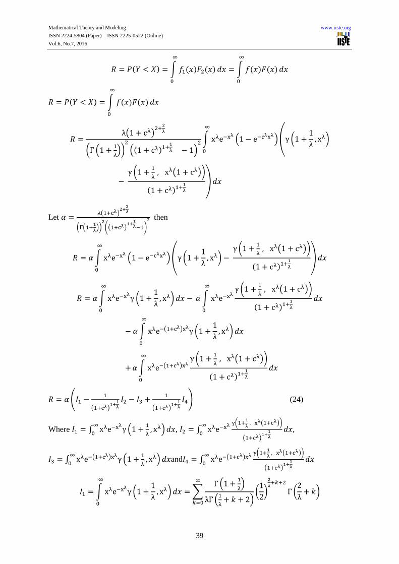
𝑅 = 𝑃(𝑌 < 𝑋) = ∫ 𝑓1(𝑥)𝐹2(𝑥)

∞

0

𝑑𝑥 = ∫ 𝑓(𝑥)𝐹(𝑥)

∞

0

𝑑𝑥

𝑅 = 𝑃(𝑌 < 𝑋) = ∫ 𝑓(𝑥)𝐹(𝑥)

∞

0

𝑑𝑥

𝑅 =λ(1 + cλ)

2+2

λ

(Γ (1 +1

λ))

2

((1 + cλ)1+1

λ − 1)2

∫ xλe−xλ(1 − e−cλxλ

) (γ (1 +1

λ, xλ)

∞

0

− γ (1 +

1

λ , xλ(1 + cλ))

(1 + cλ)1+1

λ

) 𝑑𝑥

Let 𝛼 =λ(1+cλ)

2+2λ

(Γ(1+1

λ))

2

((1+cλ)1+

1λ−1)

2 then

𝑅 = 𝛼 ∫ xλe−xλ(1 − e−cλxλ

) (γ (1 +1

λ, xλ) −

γ (1 +1

λ , xλ(1 + cλ))

(1 + cλ)1+1

λ

)

∞

0

𝑑𝑥

𝑅 = 𝛼 ∫ xλe−xλγ (1 +

1

λ, xλ) 𝑑𝑥 −

∞

0

𝛼 ∫ xλe−xλγ (1 +

1

λ , xλ(1 + cλ))

(1 + cλ)1+1

λ

𝑑𝑥

∞

0

− 𝛼 ∫ xλe−(1+cλ)xλγ (1 +

1

λ, xλ) 𝑑𝑥

∞

0

+ 𝛼 ∫ xλe−(1+cλ)xλγ (1 +

1

λ , xλ(1 + cλ))

(1 + cλ)1+1

λ

𝑑𝑥

∞

0

𝑅 = 𝛼 (𝐼1 −1

(1+cλ)1+

1λ

𝐼2 − 𝐼3 +1

(1+cλ)1+

1λ

𝐼4) (24)

Where 𝐼1 = ∫ xλe−xλγ (1 +

1

λ, xλ) 𝑑𝑥

∞

0, 𝐼2 = ∫ xλe−xλ γ(1+

1

λ , xλ(1+cλ))

(1+cλ)1+

1λ

𝑑𝑥∞

0,

𝐼3 = ∫ xλe−(1+cλ)xλγ (1 +

1

λ, xλ) 𝑑𝑥

∞

0and𝐼4 = ∫ xλe−(1+cλ)xλ γ(1+

1

λ , xλ(1+cλ))

(1+cλ)1+

1λ

𝑑𝑥∞

0

𝐼1 = ∫ xλe−xλγ (1 +

1

λ, xλ) 𝑑𝑥

∞

0

= ∑Γ (1 +

1

λ)

λΓ (1

λ+ 𝑘 + 2)

∞

𝑘=0

(1

2)

2

λ+𝑘+2

Γ (2

λ+ 𝑘)




Vol.6, No.7, 2016

40

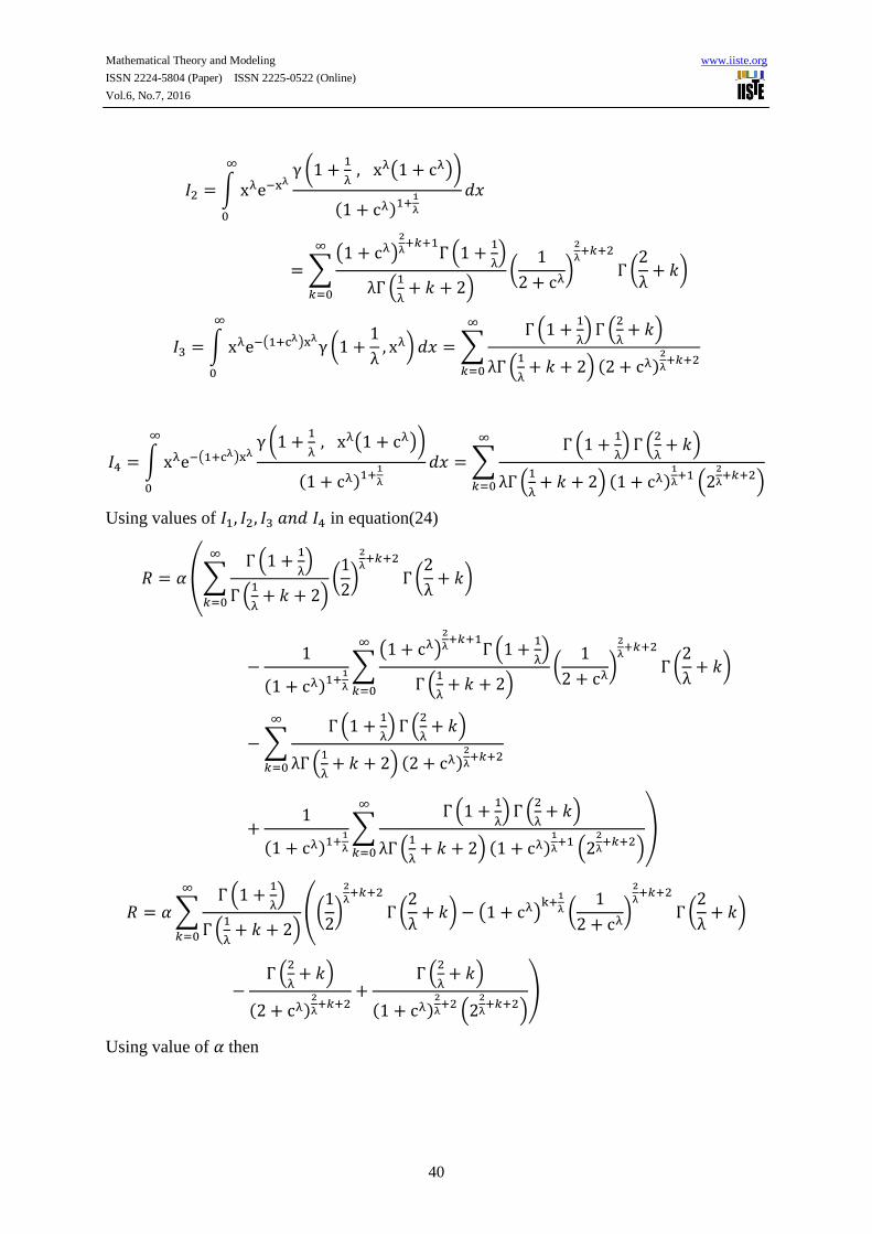
𝐼2 = ∫ xλe−xλγ (1 +

1

λ , xλ(1 + cλ))

(1 + cλ)1+1

λ

𝑑𝑥

∞

0

= ∑(1 + cλ)

2

λ+𝑘+1

Γ (1 +1

λ)

λΓ (1

λ+ 𝑘 + 2)

∞

𝑘=0

(1

2 + cλ)

2

λ+𝑘+2

Γ (2

λ+ 𝑘)

𝐼3 = ∫ xλe−(1+cλ)xλγ (1 +

1

λ, xλ) 𝑑𝑥

∞

0

= ∑Γ (1 +

1

λ) Γ (

2

λ+ 𝑘)

λΓ (1

λ+ 𝑘 + 2) (2 + cλ)

2

λ+𝑘+2

∞

𝑘=0

𝐼4 = ∫ xλe−(1+cλ)xλγ (1 +

1

λ , xλ(1 + cλ))

(1 + cλ)1+1

λ

𝑑𝑥

∞

0

= ∑Γ (1 +

1

λ) Γ (

2

λ+ 𝑘)

λΓ (1

λ+ 𝑘 + 2) (1 + cλ)

1

λ+1 (2

2

λ+𝑘+2)

∞

𝑘=0

Using values of 𝐼1, 𝐼2, 𝐼3 𝑎𝑛𝑑 𝐼4 in equation(24)

𝑅 = 𝛼 (∑Γ (1 +

1

λ)

Γ (1

λ+ 𝑘 + 2)

∞

𝑘=0

(1

2)

2

λ+𝑘+2

Γ (2

λ+ 𝑘)

−1

(1 + cλ)1+1

λ

∑(1 + cλ)

2

λ+𝑘+1

Γ (1 +1

λ)

Γ (1

λ+ 𝑘 + 2)

∞

𝑘=0

(1

2 + cλ)

2

λ+𝑘+2

Γ (2

λ+ 𝑘)

− ∑Γ (1 +

1

λ) Γ (

2

λ+ 𝑘)

λΓ (1

λ+ 𝑘 + 2) (2 + cλ)

2

λ+𝑘+2

∞

𝑘=0

+1

(1 + cλ)1+1

λ

∑Γ (1 +

1

λ) Γ (

2

λ+ 𝑘)

λΓ (1

λ+ 𝑘 + 2) (1 + cλ)

1

λ+1 (2

2

λ+𝑘+2)

∞

𝑘=0

)

𝑅 = 𝛼 ∑Γ (1 +

1

λ)

Γ (1

λ+ 𝑘 + 2)

∞

𝑘=0

((1

2)

2

λ+𝑘+2

Γ (2

λ+ 𝑘) − (1 + cλ)

k+1

λ (1

2 + cλ)

2

λ+𝑘+2

Γ (2

λ+ 𝑘)

−Γ (

2

λ+ 𝑘)

(2 + cλ)2

λ+𝑘+2

+Γ (

2

λ+ 𝑘)

(1 + cλ)2

λ+2 (2

2

λ+𝑘+2)

)

Using value of 𝛼 then




Vol.6, No.7, 2016

41

𝑅 =

∑(1+cλ)

2+2λ

Γ(1+1

λ)((1+cλ)

1+1λ−1)

2

Γ(1

λ+𝑘+2)

∞𝑘=0 ((

1

2)

2

λ+𝑘+2

Γ (2

λ+ 𝑘) − (1 + cλ)

k+1

λ (1

2+cλ)

2

λ+𝑘+2

Γ (2

λ+

𝑘) −Γ(

2

λ+𝑘)

(2+cλ)2λ

+𝑘+2+

Γ(2

λ+𝑘)

(1+cλ)2λ

+2(2

2λ

+𝑘+2)

) (25)

10 Estimation of Parameter

In this section, we obtain the maximum likelihood estimate (MLE) and method of

moment estimator (MME) for the parameters λ and c of the (DWWD).

10.1 Method of moments

From method of moment we have:

E(xk) =1

n∑ xi

k k = 1,2ni=1

For k = 1 E(x) = ∑xi

n

ni=1 = X

Γ(1+

k+1

λ)

Γ(1+1

λ)(∈−1)

(∈ −1

∈1) = X (26)

For k = 2E(x2) =1

n∑ xi

2ni=1

Γ(1+

k+1

λ)

Γ(1+1

λ)(∈−1)

(∈ −1

∈2) =

1

n∑ xi

2ni=1 (27)

Where ∈1= (1 + cλ)1

λ, ∈2= (1 + cλ)2

λ and ∈= (1 + cλ)1+

1

λ

Solving the equation (21) and (22) using numerical method we get the c and λ as estimate of

c and λ.

10.2 Maximum Likelihood Estimators

Maximum Likelihood Estimator is most effective and efficient methods for estimation of

parameters. The pdf of the DWWD is given by:




Vol.6, No.7, 2016

42


1+1λxλe−xλ

(1−e−cλxλ)

Γ(1+1

λ)((1+cλ)

1+1λ−1)

x ≥ 0, c > 0

Let 1 + cλ = α then above pdf can be written as:

fw(x; α, λ) =λ(α)

1+1λxλe−xλ

(1−e−(α−1)xλ)

Γ(1+1

λ)((α)

1+1λ−1)

x ≥ 0, α > 0 (28)

Let x1 , x2 , … , xn) be the random sample of double weighted Weibull distribution then

log-likelihood function of above pdf is given as:

L(x; c, λ) = nlogλ + n (1 +1

λ) log(α) + λlogx − xλ + log (1 − e−(α−1)xλ

)

− n log (Γ (1 +1

λ)) − nlog ((α)1+

1

λ − 1)

Differentiating w.r.t x; to λ and α we get:

∂

∂λ(L(x; α, λ)) =

n

λ−

n

λ2 log α + logx − xλlogx +(α−1) log(x)xλe−(α−1)xλ

1−e−(α−1)xλ

+n

λ2 psi (1 +1

λ) +

n(α)1+

1λlog (α)

λ2((α)1+

1λ−1)

(29)

∂

∂λ(L(x; α, λ)) =

n

α(1 +

1

λ) +

xλe−(α−1)xλ

1−e−(α−1)xλ −n(1+

1

λ)(α)

1λ

((α)1+

1λ−1)

(30)

Equating above equation to zero we get

n

λ−

n

λ2 log α + logx − xλlogx +(α−1) log(x)xλe−(α−1)xλ

1−e−(α−1)xλ +n

λ2 psi (1 +1

λ) +

n(α)1+

1λ log(α)

λ2((α)1+

1λ−1)

= 0(31)

n

α(1 +

1

λ) +

xλe−(α−1)xλ

1−e−(α−1)xλ −n(1+

1

λ)(α)

1λ

((α)1+

1λ−1)

= 0 (32)

To estimate λ and α we have to solve (25) and (26) using numerical technique methods

because it is not possible to solve analytically (25) and (26). We use newton Raphson method

to (see Adi (1966)) to obtain the solution of nonlinear equations given above.




Vol.6, No.7, 2016

43

11 Application

In this section, we are considering the lifetime data of 20 electronic components given by

Nasiru (2015))to demonstrate the application of the double weighted Weibull distribution.

The data set is given by:

0.03 0.22 0.73 1.25 1.52 1.80 2.38 2.87 3.14 4.72

0.12 0.35 0.79 1.41 1.79 1.94 2.40 2.99 3.17 5.09

The data set can be modelled by Double weighted Weibull distribution and also we can find

the estimate of parameters 𝛂and 𝛌using Newton Raphson method beginning with the initial

guess 𝛂 = 𝟏 and 𝛌 = 𝟎. 𝟕. The estimated values of the parameters are �� = 𝟎. 𝟗𝟔𝟒𝟓 and

�� = 𝟑𝟎𝟑. 𝟎𝟔𝟔𝟖 after 21 iterations.Teimouri and Gupta (2013) also studied this data using a

three-parameter Weibull distribution. In this study, the double weighted Weibull distribution

is fitted to this data and the results are compared to Weibull distribution using well-known

goodness test of statistics, Kolmogorov-Smirnov (K-S) test. The results of Kolmogorov-

Smirnov (K-S) test are given in the table below as:

Table 2. Parameter estimates and K-S statistics for 20 electronic components

Distributions WD DWWD

Parameters estimates α= 1.0792

λ = 0.9645

α = 303.0668

K.S statistics 0.3698 0.1516

P values < 0001 0.2460

From above table the DWWD has greater p value as compared to the WD which claims that

DWWD gives better fit the 20 electronic components data set from WD. Only the K-S test is

not satisfactory statistical indication for supporting that the data set do not closely fitted by

the WD. My second judgement based on graphical test as shown in figure7 which represent

that the densities of the theoretical distributions WD and DWWD plotted over the empirical

histogram of 20 electronic components data. Figure3 indicate that DWWD is more fitted to

these data as compared to WD.




Vol.6, No.7, 2016

44

Figure 3. The plot b/w theoritical distributions and emperical histogram for data of 20

electronic components

12 Conclusion

This paper develops a new double weighted distribution known as double weighted Weibull

distribution DWWD. The statistical properties mean, variance, coefficient of variance and

standard deviations are also determined of DWWD. The data set validate the fitting of the

proposed distribution DWWDas compared to WD using a well-known Kolmogrov-Smirnov

test. The results of the K-S statistics indicate that the DWWD is suitable as compared to

WD.Our proposed distribution DWWD is more general modal because existing double

weighted distributions (Double weighted Religh distribution and double weighted

exponential distribution) are special cases to our proposed distribution DWWD (See section

4).

References

Ahmed, A., Mir, K. A.,Rashi, J. A. (2013). On new method of estimation of parameters of

size-biased generalized gamma distribution and its structural properties. IOSR J.

Math. 5: 34-40.




Vol.6, No.7, 2016

45

Al-khadim, K. A.,Hantoosh, A. F.(2013). Double Weighted distribution and double

weighted exponential distribution. Mathematical theory and Modling, Vol.3:124-134.

Al-khadim, K. A.,Hantoosh, A. F. (2014). Double Weighted Inverse Weibull distribution,

Malaysia Handbook on the Emerging Trends in Scientific Research, ISBN: 978-969-

9347-16-0.

Almalki, S. J., Yuan, J. (2013). The new modified Weibull distribution.Reliability

Engineering and System Safety.111: 164-170.

Al-Saleh, J. A.,Agarwal, S. K. (2006). Extended Weibull type distribution and finite

mixture of distributions.Statistical Methodology, 3:224-233.

Ben-Israel A (1966). Newton-Raphson Method for the Solution of Systems of equations

Equations.Journal of Mathematical analysis and applications. 15: 243-252

Das, K. K.,Roy, T. D. (2011) Applicability of length biased weighted generalized Rayleig

distribution.Advances in Applied Science Research. 2:320-327.

FisherR A (1934).The effect of methods of ascertainment upon the estimation of

frequencies.The Annals of Eugenics. 6:13-25.

Gokarna, A. R., Chris, T. P. (2011). Transmuted Weibull Distribution: A Generalization of

the Weibull Probability Distribution.European journal of pure and applied

mathematics. 4: 89-102.

Ghitany, M. E., Al-Mutairi, D. K. (2008). Size-biased Poisson-Lindley distribution and its

application.International Journal of Statistics 2008, vol. LXVI, n. 3, pp. 299-311.

JING, X. K. (2010). Weighted Inverse Weibull and Beta-Inverse Weibull distribution, 2009

Mathematics Subject Classification.62N05, 62B10.

Kishore, K., Das, K. K.,Tanusree, D. R. (2011). Applicability of Length Biased Weighted

Generalized Rayleigh Distribution, Advances in Applied Science Research, 2 (4):

320-327.

Merovci, F.,Elbatal, I. (2015).Weibull Religh distribution theory and applications.J.

Applied Mathematics and inpormation science, 4: 2127-2137.

Nanuwong, N., Bodhisuwan, W. (2014). The length-biased beta-pareto distribution and its

structural properties with application.Journal of Mathematics and Statistics,

10: 49-57.




Vol.6, No.7, 2016

46

Nasiru, S. (2015). Another weighted Weibull distribution from azzalini’s family. European

scientific journal. 11: 134-144.

Oluyede, B. O., George, E. O. (2000). On Stochastic Inequalities and Comparisons of

Reliability Measures for Weighted Distributions.Mathematical problems in

Engineering.8:1-13.

Oluyede, B. O.,Terbeche, M. (2007). On Energy and Expected Uncertainty Measures in

Weighted Distributions. International Mathematical Forum. 2: 947-956.

Pal, M., Ali, M. M., Woo J. (2006). Exponentiated Weibull distribution.Statistica, 66: 139-

147.

Rao, C. R. (1965) On discrete distribution arising out of methods of ascertainment, in

Classical and Contagious Discrete Distribution, G.P. Patil, ed., Pergamon Press and

Statistical Publishing Society, Calcutta, pp.320-332.

Rishwan, N. I. (2013).Double Weighted Rayleigh Distribution Properties and Estimation.

International Journal of Scientific & Engineering Research. Vol. 4, Issue 12, ISSN

2229-5518.

Seenoi, P., Supapakorn, T.,Winai, B. (2014). The length-biased Exponentiated inverted

Weibull distribution. International Journal of Pure and Applied Mathematics.

92: 191-206.

Teimouri, M., Gupta, K. A. (2013). On three-parameter Weibull distribution shape

parameter estimation. Journal of Data Science.11: 403-414.

Xie, M.,Lai, C. D. (1996). Reliability analysis using an additive Weibull model with

bathtub shaped failure rate function. Reliability Engineering andSystem Safety.52(1):

87-93.


Double Weighted Weibull Distribution Properties and ... - IISTE's

Documents

Transcript of Double Weighted Weibull Distribution Properties and ... - IISTE's