The Weighted Proportional Allocation Mechanism

Thành NguyenNorthwestern University

Evanston, IL, USAthanh@eecs.northwestern.edu

Milan VojnovicMicrosoft Research

Cambridge, UKmilanv@microsoft.com

October 2010

Technical ReportMSR-TR-2010-145

Microsoft ResearchMicrosoft CorporationOne Microsoft Way

Redmond, WA 98052http://www.research.microsoft.com

Abstract–We consider a weighted proportional allocation of resources that allows providers to discriminate us-age of resources by users. This framework is a generalization of well-known proportional allocation accommodatingallocation of resources proportional to weighted bids or proportional to submitted bids but with weighted payments.

We study a competition game whereeveryone is selfish: providers choose discrimination weights aiming atmaximizing their individualrevenueswhile users choose their bids aiming at maximizing their individual payoffs.We analyze revenue and social welfare of this game. We find that the revenue is lower bounded byk/(k+1) timesthe revenue under standard price discrimination scheme, where a set ofk users is excluded. For users with linearutility functions, we find that the social welfare is at least1/(1+ 2/

√3) of the maximum social welfare (approx.

46%) and that this bound is tight. We extend the efficiency result to a broad class of utility functions and to multiplecompeting providers. We also describe an algorithm used by the provider to adjust the user discrimination weightswithout a prior knowledge of user utility functions and establish convergence to equilibrium points of our game.

Our results show that, in many cases, weighted proportionalsharing achieves competitive revenue and socialwelfare, despite the fact that everyone is selfish. The mechanism allows for resource constraints described by generalpolyhedrons, thus accommodating a variety of resources, including bandwidth of communication networks, systemsof computing resources, and sponsored search ad slots.

1 Introduction

Auctions-based Resource Allocations. Provisioning of computer systems and services usinga pay-per-use pricinghas proliferated over recent years. For example, major providers of cloud computing services use either fixed pricesor auctions to sell compute instances. The two forms of saleshave their own advantages and disadvantages. Whilefixed price schemes are simple to implement, in many scenarios they are not robust and not very flexible. For instancewhen the users’ demands are inelastic, a small change in prices can translate to a dramatic change in the demandsthat can cause congestion and system failure. Furthermore,in order to update prices, providers usually need togather enough data from sales, this inflexibility can cause inefficiency for the systems and result in low revenues.In recent years, using auction-based schemes for allocating and selling resources in computing systems has becomemore popular. Sales using auctions are known to be more flexible and can extract information from users faster. Thefact that both users and providers can adjust their bids and parameters in auctions in a more dynamic way reflectsin the tremendous improvement of the system efficiency or therevenue obtained by the providers. Moreover, thedisadvantages of the auction-based approaches such as, thedifficulties for users to find optimal strategies and forproviders to change their platforms, have been greatly improved in recent years with availability of software thathelps users to optimize the bidding strategies and several online services offering auction platforms.

Examples of using auctions for resource allocation includeselling of Amazon EC2 spot instances [1]; selling ofsponsored search ad slotsto advertisers by major providers of online services and areof much interest widely acrossengineering systems, includingelectricity markets[26] that have been gaining momentum due to a pressing need toaccommodate renewable energy sources. Furthermore, numerous auction-based proposals for allocation of systemresources have been made such as allocation of disk I/O in storage systems [7] and allocation of computationalresources [4] and it was even showed that sharing of network resources in the Internet by TCP connections may beseen as an auction [13, 11].

Discriminative Schemes in Auctions-based Allocations. It is well known that in practice with fixed price schemesproviders usually apply different prices to different users for selling identical goods or services. This scheme, oftencalled price discrimination, is very common in practice. Itis not surprising that similar discriminative schemes arealso used extensively in auction-based allocations. Thereare two main reasons for such a discriminative framework.First, different users require different subsets of resources owned by the provider (e.g. transmission rate for differentpaths through a network), thus, by discriminating among users the provider can improve the efficiency of the system.Second, different users have different valuations of the amount of resource received (e.g. different valuation oftransmission rates); in this case, the providers once having learned this information can try to take advantage anduse discrimination to improve the revenue.

The most well known example of auctions using such a discrimination scheme is the generalized second price

1

replacements

P PP

C

C

C

C

C

C1

C1

C2

C2

C2

C3

C3

x1

x1x1

x1

x1

x1

x2

x2

x2

x2

x2

x2

C/w

C/w

ww

1

1

Figure 1: Examples of polyhedron constraints: (left) single link, (middle) a network of links, (right) assignmentcosts of a workflow to machines.

auction currently used by search engines to allocate ads. Inthis mechanism, the providers assigns different weightsto different users (advertisers) and the mechanism is run based on weighted bids.

The Framework. In this paper, we consider a class of auctions that allows providers to discriminate among differentusers. Specifically, we are interested in auctions that are simple in terms of the information provided by users, andare easy to describe to users. We consider two natural instances of weighted proportional allocation: (1)weighted bidauctionwhere the allocation to a user is proportional to the bid submitted by this user weighted with a discriminationweight that is selected by the provider, and the payment by the user is equal to his own bid, and (2)weighted paymentauctionwhere the allocation to a user is proportional the bid of thisuser and the payment is equal to the weightedbid, where the weight is selected by the provider. The weighted bid auction is a novel proposal while weightedpayment auction was recently proposed by Ma et al [18].

As in the network pricing literature [20], we consider theseallocation problems in thefull information setting.The justification for this setting is the fact that in practice allocation auctions are run repeatedly and thus, providerscan learn about the behavior and private information of users. As discussed in the beginning of this section, evenin this setting there are several advantages of using proportional sharing-like auctions over fixed price schemes.Namely, both of the auctions that we consider are akin and natural generalizations of well-known proportional al-location (e.g. [13, 11, 8], see related work discussed laterin this section). Thus, this class of mechanisms inheritsmany natural properties of the traditional proportional sharing rule making iteasy and robust to implementin prac-tice. First, these mechanisms are simple for bidders, they only need to know the total of others’ bids. Second theallocation is a natural and continuous function of the bid vector, and, therefore, it can be robustly implemented in adistributed way (as will be shown later in our paper). From anengineering point of view, this is an important featureof practical allocation rules. For example, when users demands are inelastic (users’ utilities are close to linear)proportional sharing-like mechanisms are much preferred to fixed price schemes.

Another important reason that motivates us to study these weighted proportional rules is the fact that in settingswhere providers’ goal is tomaximize revenue, the weighted proportional sharing is preferred over the traditionalproportional sharing. As will be shown later, while weighted proportional sharing always generates near-optimalrevenue, the revenue of traditional proportional sharing provides no such guarantee, and in fact, can be arbitrarilybad.

We study these allocation rules ingeneral convex environmentsthat capture many special cases of resourceallocation problems such as the network bandwidth sharing,sponsored search, and scheduling of resources in cloudcomputing (see Figure 1 for an illustration). We provide a deeper discussion of these applications in Appendix A.We consider a provider that offers a resource to a set of usersU = {1,2, . . . ,n} wheren≥ 1 (for the case of multipleproviders, the auctions as described in the following are applied by each individual provider). We denote with~x= (x1,x2, . . . ,xn) and~q=(q1,q2, . . . ,qn) the vector of allocations and payments by users, respectively. The resourceowned by the provider is allowed to be an arbitrary infinitelydivisible resource with constraints specified by a convexset, sayP ∈ IRn

+. An allocation vector~x is said to befeasibleif ~x∈ P . The provider discriminates users by assigningadiscrimination weight Ci ≥ 0, for every useri. Each useri, submits a bidwi ≥ 0.

Our weighted bid auction determines the allocation and payment for each user as follows:

2

WEIGHTED BID AUCTION

For useri with bid wi :

Allocation xi =Ciwi

∑ j∈U wj

Payment qi = wi

where discrimination weights~C are chosen such that~x is feasible. We may interpret the discrimination weightCi

as the maximum allocation determined by the provider for user i and xi is the actual allocation set to a fractionwi/∑ j∈U w j of this user-specific maximum allocation.

On the other hand, the weighted payment auction determines the allocation and payment by each user as givenin the following:

WEIGHTED PAYMENT AUCTION

For useri with bid wi :

Allocation xi =C wi∑ j∈U wj

Payment qi =Ciwi

whereC is the maximum allocation to a user and the discrimination weight Ci determines the payment by useri.Compared with the traditional proportional allocation, the weighted bid auction is more suitable for general

convex resource constraints. This is not the case for weighted payment auction; while the relative allocation acrossusers can be arbitrary by appropriate choice of user bids, the implicit assumption of the allocation rule is that∑i xi = C, i.e. the provider is required to a priori commit to allocating a total amount of resourceC > 0. Whilethis is not restrictive for allocating an infinitely divisible resource of capacityC > 0, this allocation rule cannotaccommodate more general polyhedral constraints. Thus, inthis paper we will mainly focus on the weighted bidauction but also consider some properties of the weighted payment one as it is an alternative auction that allows foruser discrimination, though for special type of resource constraints.

Questions Studied in this Paper. We consider a general competitive setting with multiple providers and userswhereeveryone is selfish: each provider aims at maximizing own revenue and each user aims at maximizing ownpayoff. Ideally, an allocation mechanism would guarantee high revenueto a provider and highefficiencywhere byefficiency we mean social welfare (i.e. the total utility across all users) compared with best possible social welfare.In a competitive setting where everyone is selfish, it is rather unclear whether the two goals could be simultaneouslyachieved. Intuitively, one would expect that selfishness ofusers and providers may well result in either poor revenueor efficiency. For example, providers that aim at maximizingtheir revenue may well have an incentive to misreportavailability of their resources1. Our main questions in this paper are:

Q1: How much revenue can a provider obtain using weighted proportional sharing rules?

Q2: What is the efficiency loss in the complex system where everyone is selfish?

Overview of our Results. Our results can be summarized in the following points:• Revenue: We show that the revenue of weighted bid auction is at leastk/(k+ 1) times the revenue under

standard price discrimination scheme with a set ofk users excluded, which we describe in more detail in Section 3.The comparison of the revenue of a mechanism with maximum revenue obtained under another optimal pricingscheme where some users are excluded is standard in the mechanism design literature (e.g. [9]) and our revenuecomparison result is novel and of general interest. The result enables us to understand conditions under which therevenue of weighted bid auction is competitive to that underthe benchmark pricing scheme, e.g. the case of manyusers.

1A famous example of such a market manipulation isCalifornia electricity criseswhere, in 2000 and 2001, there was a shortage ofelectricity because energy traders were gratuitously taking their plants offline at peak demand in order to sell at higher prices [27].

3

• Efficiency: We establish that for linear user utility functions, weighed bid auction guarantees the social welfareof at least 1/(1+2/

√3) ≈ 0.46 times the maximum social welfare (price of anarchy), and this bound is tight. We

also show a tight efficiency bound of 1/2 for the weighed payment auctions. We extended our efficiency result ofthe weighed bid auction to a broad class of utility functions, we callδ-utility functions, whereδ ≥ 0. We show thatmany utility functions found in literature areδ-utility functions, in many cases withδ ≤ 2, and show that this classof utility functions is closed to addition and multiplication with a positive constant. We then show that if the utilityfunctions areδ-utility functions, then the social welfare is at least 1/(1+ 2/

√3+ δ) times the maximum social

welfare, and establish that this guarantee holds for a system of multiple competing providers. A similar extensionfor the weighted payment auction is also shown.

• Convergence and distributed algorithms: We demonstrate how a provider can adjust discrimination weightsin an online fashion so that allocations and payments converge to Nash equilibrium points of the competition gamethat we study. This shows that the information about user utility functions needed by the provider can be estimatedfrom the bids submitted by users in an online fashion. We describe a distributed iterative scheme and the estimationneeded, and prove convergence to Nash equilibrium for the case of linear user utility functions.

Finally, we note that our results also provide insights on the performance of systems where providers wouldclaim to use traditional proportional allocation but then strategically manipulate the information signaled to userswith the aim to earn higher revenue.

Related Work. The concept of allocating resources proportional to user-specific weights has a long and rich historyin the context of computer systems and services. For example, it underlies the objective of generalized proces-sor sharing [21, 2], sharing of bandwidth in communication networks [13], has been considered for allocation ofstorage [7] and compute instances [4]. Our weighted bid auction could be seen as a generalization of traditionalproportional allocation that allows to discriminate usersand accommodates general convex resource constraints.

Previous work primarily focused on analyzing social efficiency of proportional allocation in competitive envi-ronments where only users are assumed to be selfish. Kelly [13] established that under price taking users that submita single bid for a set of resources of interest (e.g. allocation of bandwidth at each link along a path of a networkconnection), the proportional allocation guarantees 100%efficiency. In a subsequent work, Johari and Tsitsiklis [11]showed that the social efficiency is at least 75% under price anticipating users and assumption that each user submitsan individual bid for each individual resource of interest (e.g. a bid submitted for each link along a path of a networkconnection). The latter result was extended by Nguyen and Tardos [19] for more general polyhedral constraints.Finally, Yang and Hajek [8], in turn, showed that the worst-case efficiency is 0% if users are restricted to submittinga single bid for a set of resources of interest. Our work stands in contrast to this line of work in that we consider acompetitive environment where everyone is selfish.

The weighted payment auction studied in this paper was first proposed by Ma et al [18] where they focused onmaximizing social welfare. We provide revenue and efficiency results for weighted payment auctions in environ-ments where everyone is selfish.

Our setting of multiple providers bears quite similarity with that found in the context of ISP multihoming (e.g. [6,22, 10]) and to that of multi-path congestion control, e.g. [5], and may also inform about competition in time-varyingmarkets using the approach in [15].

Outline of the Paper. Section 2 introduces the resource competition game more precisely. Section 3 presents ourmain revenue comparison result (Theorem 1). In Section 4, wepresent our results on the efficiency guarantees forthe case of a single provider and users with linear utility functions (Theorem 2). Section 5 extends the efficiencyresult to more general class of user utility functions and more general setting of multiple providers (Theorem 4). Wediscuss convergence to Nash equilibrium points and distributed schemes in Section 6. In Section 7, we conclude.Some of the proofs are presented in Appendix.

2 The Resource Allocation Game where Everyone is Selfish

We consider a system ofn users competing for resources of a single provider; we introduce the setting with multipleproviders later in Section 5.1. Recall that~x= (x1,x2, . . . ,xn) and~q= (q1,q2, . . . ,qn) denote the vector of allocations

4

and payments by users, respectively. The allocation vector~x is feasible only if~x∈ P whereP is a set inRn+. We

assume thatP is a convex set of the formP = {~x ∈ IRn+ : A~x ≤~b} for some matrixA and a vector~b with non-

negative elements. (Note thatA and~b can have arbitrarily many rows, so we refer to “convex” constraints, insteadof to polyhedrons.)

Suppose thatUi(xi) is the utility of allocationxi to useri. Throughout this paper we assume that for everyi, Ui(x)is a non-negative, non-decreasing and continuously differentiable concave function. The payoffs for the provider andusers are defined as follows. The payoff of the provider is equal to the revenue, i.e. the total payments received fromall users,R= ∑i qi . On the one hand, the payoff for a useri is equal to the utility minus the payment, i.e.Ui(xi)−qi

for allocationxi and paymentqi for useri.The competition game that we study can be seen as the following two-stage Stackelberg game: in the first stage,

the provider announces the discrimination weights~C and then, in the second stage, users adjust their bids in a selfishway aiming at maximizing their individual payoffs. In the first stage, the provider anticipates how users would reactto given discrimination weights~C and sets them in a selfish way aiming at maximizing own revenue. In dynamicsetting, the two stages of this game would alternate over time (we discuss this in Section 6).

In the reminder of this section we characterize Nash equilibrium for weighted-bid and weighted-payment auc-tion.

Equilibrium of Weighted Bid Auction . We show a relation between the revenue gain and the allocation of anoutcome. Given a discrimination weightCi and the sum of the bids∑ j w j , each useri selects a bidwi that maximizeshis surplus, i.e. solves

USER: maxwi≥0

Ui

(

wi

∑ j 6=i w j +wiCi

)

−wi. (1)

Under the assumed behavior of users, one can analyze the Nashequilibrium of the game. It turns out that a Nashequilibrium exists and is unique, and at Nash equilibrium the relation between revenue and allocation is captured byan implicit function.

For the provider, he would like to choose the rate to maximizethe revenue. We first show the following relationbetween the revenue and the allocation vector~x.

Lemma 1 Given discrimination weights~C, there is a unique allocation~x corresponding to the unique Nash equilib-rium. Conversely, given an allocation~x, there is a weight~C such that~x is the corresponding outcome. Furthermore,the corresponding revenue R(~x) is a function of~x given by

∑i

U ′i (xi)xi

U ′i (xi)xi +R(~x)

= 1. (2)

Given this result, we obtain the following optimization problem of the provider.

PROVIDER: maximizeR(~x) over~x∈ P . (3)

In the rest of this section we provide a proof of Lemma 1.

of Lemma 1 We havexi =Ci

wi

∑ j w j(4)

and USER problem can be written as:

maximizeUi

(

wi

∑ j 6=i w j +wiCi

)

−wi overwi ≥ 0. (5)

Note that the objective function in (5) is concave inwi, hence, at an optimum solution eitherwi = 0 or the derivativeof the objective function is zero. Setting the derivative tozero is equivalent to:

U ′i (xi) ·Ci

∑ j 6=i w j

(∑ j w j)2 = 1, for xi > 0.

5

It follows

U ′i (xi) =

(∑ j w j)2

Ci ∑ j 6=i w j=

R2

Ci(R−wi)(6)

where recall the revenue is equal to the sum of the payments byindividual users, i.e.R= ∑ j w j . Combining withwi = xiR/Ci that follows from (4), we have

U ′i (xi) =

RCi −xi

⇔CiU′i (xi)(1−

xi

Ci) = R. (7)

Now, ∑ xiCi= 1, thus, condition (7) is exactly the condition for maximizing

∑i

∫ xi

0CiU

′i (ti)

(

1− tiCi

)

dti

over~x∈ IRn+ and subject to∑ xi

Ci= 1.

Since∫ xi

0 CiU ′i (ti)

(

1− tiCi

)

dti is a strictly concave function with respect toxi , there exists a unique Nash equilibrium.

It remains to show that for an equilibrium allocation~x, the revenueR is given by

∑i

U ′i (xi)xi

U ′i (xi)xi +R

= 1. (8)

From (7), we have

U ′i (xi) =

RCi −xi

=R

xi(Ci/xi −1)⇒ Ci

xi−1=

RU ′

i (xi)xi

⇒ xi

Ci=

U ′i (xi)xi

U ′i (xi)xi +R

.

Combining with∑i xi/Ci = 1 which follows from (4), we obtain (8). Note that all the formulas above are appliedfor the casexi > 0 only; nevertheless, ifxi = 0, we haveU ′

i (xi)xi = 0, and therefore, the equation (8) holds for anyoptimum allocation vector~x.

Finally, we note that in equilibrium, the vector of discrimination weights~C and the vector of bids~w are functionsof the equilibrium allocation~x given as follows: for everyi,

Ci = xi +R(~x)

U ′i (xi)

andwi =R(~x)

U ′i (xi)xi +R(~x)

U ′i (xi)xi .

Equilibrium of Weighted Payment Auction . The analysis follows similar steps as for the weighted bid auction; inthis case the revenue at Nash equilibrium can be representedas an explicit function of the allocation vector~x. Givena discrimination weightCi , useri solves the following surplus maximization problem:

USER: maxwi≥0

Ui

(

wi

∑ j 6=i w j +wiC

)

−Ciwi. (9)

Lemma 2 Given a vector of discrimination weights~C, there is a unique allocation~x corresponding to the uniqueNash equilibrium. Conversely, given an allocation~x, such that∑i xi = C, there is a vector~C of discriminationweights such that~x is an outcome. Furthermore, the corresponding revenue R(~x) is given by

R(~x) = ∑i

U ′i (xi)xi

(

1− xi

C

)

.

6

Proof. For the USER problem (9) we have that eitherwi = 0 or the derivative of the objective function is zero, i.e.

U ′i (xi)

∑ j w j −w j

(∑ j w j)2 −Ci = 0.

Combining with the allocation rule of weighted bid auction,it is easy to observe that the last equality is equivalentto

U ′i (xi)

C−xi

∑ j w j=Ci.

Therefore,R= ∑

i

Ciwi = ∑i

U ′i (xi)(C−xi)

wi

∑ j w j

which combined withxi = Cwi/∑ j w j yields the asserted revenue in the lemma. It is straightforward to see thatgiven~x such that∑i xi =C, we can findCi andwi such that the condition of the Nash equilibrium is satisfied at~x.

3 Revenue

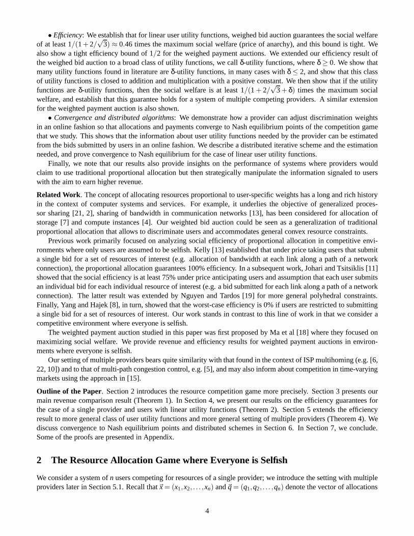
Revenue of Traditional Proportional Sharing. We demonstrate poor performance of traditional proportional shar-ing with respect to revenue for the example of a parking-lot network that is a canonical example used in the contextof networking (Figure 2). The resource consists of a series of n ≥ 1 links, each of a capacityC > 0 (without lossof generality we assumeC = 1). The example consists ofn+ 1 users; user 0 is amulti-hop userthat requires aconnection through links 1,2, . . . ,n while a useri is asingle-hop userthat requires a connection through linki, fori = 1,2, . . . ,n. User utility functions are assumed to beα-fair, i.e. for α > 0 andα 6= 1, we haveUi(x) =

wαi

1−αx1−α,andUi(x) = wi log(x), for α = 1, wherewi > 0 (in our example, we consider a symmetric case wherewi = 1, forevery useri). The resource constraints in this example arexi +x0 ≤ 1, for every linki = 1,2, . . . ,n.

x0

x1 x2 xn

· · ·

Figure 2: Parking-lot example.

Under proportional sharing mechanism, user 0 submits a bid for each ofn links while useri, i = 1,2, . . . ,n, onlybids for the linki. Using the known conditions for Nash equilibrium of the game(e.g. [11, 19]), one can show thatthere is a unique equilibrium that is a solution of the following problem:

maximizen

∑i=0

∫ xi

0U ′

i (y)(1−y)dy

over~x∈ IRn+1+

subject toxi +x0 ≤ 1, i = 1,2, . . . ,n.

Furthermore, the revenue at Nash equilibrium allocation~x is the sum of all the bids on every links. As shown in [19],on link i, the total bid is equal toU ′

i (xi)(1−xi), thus the revenue of the traditional proportional sharing mechanism is∑n

i=1U ′i (xi)(1−xi). For our example, by a straightforward calculation, one canshow that Nash equilibrium allocation

is x0 for user 0 and 1−x0 for each useri = 1,2, . . . ,n, wherex0 =1

1+n1/(α+1) . The revenue of this mechanism isnx0(1−x0)α .

For large network sizen, it is not difficult to observe that the revenue isO(nα

α+1 ). Hence, the revenue iso(n) for everyfixedα> 0. The intuition behind why the revenue is low is quite clear;for large network sizen, user 0 has to competewith many users, therefore, the payment on each link that this user can afford is becoming smaller. Consequently,

7

the competition at each link is reduced. If, on the other hand, a fixed price scheme is used, the provider can charge aunit price on each link and receive a revenue ofn.

The question that we investigate in this section is how much revenue the weighted bid auction can achieve incomparison with a best fixed price scheme (with discrimination). We will answer this question in the remainder ofthis section.

Revenue of Weighted Bid Auction. We will compare the revenue of weighted bid auction with that of a benchmarkthat uses a standard fixed-price scheme [24]. In this pricingscheme, the provider charges user-specific prices per unitof resource for different users. Supposepi is the price per unit of resource for useri, then useri surplus maximizationproblem is maxUi(xi)− pixi overxi ≥ 0. The solution of this problem is given byU ′

i (xi) = pi . Therefore, the revenueof the provider isR= ∑i pixi = ∑i U

′i (xi)xi , and thus the optimal revenue isR∗ = max{∑i U

′i (xi)xi :~x∈ P}.

However, comparing with such a benchmark would be too ambitious because with auction-based allocation theprovider cannot announce fixed prices, but instead the prices are induced from the demand of users. Thus, instead,we will compare our revenue withR∗ in a setting wheresome users are excluded. That is, we will compare therevenue achieved by an auction forn users with the revenue achieved by fixed prices forn−k users, for 0< k< n.We note that this is a standard way of revenue comparison in the theory of auctions [9].

In the parking-lot example introduced above, if we considern large enough, then the optimal revenue is of ordern, which can be achieved if the provider charges every single-hop user a unit price of 1 and charges the multi-hopuser a unit price ofn. Now, if we exclude an arbitrary set ofk< n users, then the optimal revenue isn−k. Therefore,if k is much smaller compared withn, then one can think of this as alarge marketsituation where the effect of thefact that a few users do not participate in the market is negligible.

Having discussed the intuition, we can now state our main result on the revenue guarantee of weighted bidauctions. LetR∗

n−k be the optimal revenue under our benchmark, i.e.

R∗n−k = min

S⊂{1,...,n}: |S|=n−kmax~x∈P

∑i∈S

U ′i (xi)xi .

The revenue guarantee of weighted bid auctions can be statedas follows.

Theorem 1 Suppose that for each i, U′i (x)x is a concave function. Let R be the optimum revenue of the weighted bidallocation mechanism, then

for every1≤ k< n : R≥ kk+1

R∗n−k.

The revenue guarantee of the theorem above is rather strong.In particular, by taking as a benchmark the systemwith just one user excluded, we obtain that the revenue underweighted bid auction is a factor 1/2 of the revenueunder standard price discrimination with one less user (whose exclusion reduced the revenue the most). Informally,the result tells us that for systems with many users with comparable utility functions, the revenue under weightedbid auction would be close to the revenue under standard price discrimination. As discussed above such a guaranteecannot be provided by traditional proportional sharing.

Proof. For R(~x) given by (2), it is easy to observe that for every~x∈ P ,

∑i

U ′i (xi)xi −max

jU ′

j(x j)x j ≤ R(~x)<∑i

U ′i (xi)xi . (10)

Suppose that for each 1≤ k< n, there exists~x∈ P such that both of the following two conditions hold

(i) ∑i U′i (xi)xi ≥ R∗

n−k;

(ii) U ′1(x1)x1 = · · ·=U ′

k+1(xk+1)xk+1 ≥ ·· · ≥U ′n(xn)xn,

where, without loss of generality, the users are enumeratedsuch thatU ′1(x1)x1 ≥ ·· · ≥U ′

n(xn)xn. Under conditions(i) and (ii), the theorem follows because

R(~x)≥ ∑i

U ′i (xi)xi −max

jU ′

j(x j)x j

≥ kk+1∑

i

U ′i (xi)xi ≥

kk+1

R∗n−k.

8

We show that such a vector~x exists by induction overk. Base step: k = 0. The vector~x that maximizes∑i U′i (xi)xi

over~x∈ P satisfies both conditions.Induction step: Let~x∈ P be a vector such that both condition (i) and condi-tion (ii) hold for k. We then show that there exists another vector inP such that these conditions hold fork+1. NotethatR∗

n−k ≥ R∗n−(k+1) as allowing to exclude a larger set of users cannot increaseR∗

n−k. In the following, without lossof generality, we assume that users are enumerated such thatU ′

1(x1)x1 ≥ ·· · ≥U ′n(xn)xn. Let~y∈ P be an optimum

solution of the provider’s problem under our benchmark pricing scheme and the constrainty1 = . . .= yk+1 = 0, i.e.with users 1,2, . . . ,k+1 excluded. We have that∑i U

′i (yi)yi ≥ R∗

n−(k+1).Now, let us consider the vector~v(t) defined by

~v(t) =(1− t) · (U ′1(x1)x1, . . . ,U

′n(xn)xn)+

+ t · (U ′1(y1)y1, . . . ,U

′n(yn)yn), for t ∈ [0,1].

Note that ast increases from 0, thek+1 largest coordinates of~v(t) decrease, while all the other coordinates eitherincrease or do not change. Thus, there existst∗ ∈ [0,1] such that the largestk+ 2 coordinates of~v(t) are equal.Furthermore, as∑i U

′i (xi)xi ≥ R∗

n−(k+1) and∑i U′i (yi)yi ≥ R∗

n−(k+1), we have that∑i vi(t∗)≥ R∗n−(k+1). Finally, since

for eachi, U ′i (xi)xi is concave, there exists a vector~z∈ P such that(U ′

1(z1)z1, . . . ,U ′n(zn)zn) =~v(t∗). By this, we

showed that the vector~zsatisfies conditions (i) and (ii) fork+1 which completes the proof.

Remark For the weighted payment auction, observe that the maximum revenue is given by

max

{

∑i

U ′i (xi)xi(1−xi/C) :~x∈ IRn

+, ∑i

xi =C

}

.

On the other hand, the optimal revenue under the price discrimination scheme is

R∗ = max

{

∑i

U ′i (xi)xi :~x∈ IRn

+, ∑i

xi =C

}

.

Therefore, givenk≥ 1, there will be at mostk users who get at leastC/k. For other users, we havexi ≤C/(k+1),thusU ′

i (xi)xi(1−xi/C) ≥ kk+1U ′

i (xi)xi . If we chooseCi such that the outcome of the game is the allocation vector~xthat maximizesR∗, we can also obtain a similar revenue lower bound for the caseof weighted pay auction with anadditional constraint thatU ′

i (xi)xi is nondecreasing.

4 Efficiency for Linear User Utility Functions

In this section, we analyze the efficiency of the system for the case of single provider and linear user utility functions.From a technical point of view, although this result is for a special class of utilities, it provides us with basictechniques for a more general result established in the nextsection.

4.1 Efficiency of Weighted Bid Auction

We show the following theorem.

Theorem 2 Assume that the provider maximizes the revenue and for each user i, the utility function is linear, Ui(x) =vix, for some vi > 0. Then, the worst-case efficiency is1/(1+ 2/

√3) (approx. 46%). Furthermore, this bound is

tight.

Remark Before proving the theorem, note that the worst-case efficiency can be achieved asymptotically as thenumber of usersn tends to infinity. One example is when we have the resource constraint ∑i xi ≤ 1, and there isa unique user with largest marginal utility, say this is user1, and all other users have identical marginal utilitiesequal to(2−

√3)2v1 ≈ 0.0718v1. At the Nash equilibrium, user 1 obtains 42.26% of the resource and the rest

9

is equally shared by the remaining users. Thus, the efficiency loss occurs only when there is an unbalance in themarginal utilities by the users. One can actually show that when there is a higher competitiveness among the users,the efficiency increases. More precisely, we show that if there are at leastk users with the largest marginal utility,then the efficiency is at least 1− 1

2k +o(1/k). The proof of this result is Appendix C.

We first need the following lemma about thequasi-concavityof the objective function optimized by the provider.Recall thatR(~x) is the function given by (2). LetR∗ be the optimum revenue, i.e.R∗ = max{R(~x) : ~x∈ P}. We notethe following fact.

Lemma 3 The setLµ := {~x∈ IRn+ : R(~x)≥ µ} is convex, for every µ∈ [0,R∗].

Proof. We want to show thatLµ := {~x∈ IRn

+ : R(~x)≥ µ}is convex, where

∑i

vixi

vixi +R(~x)= 1.

It is clear thatR(~x) is a monotone increasing function in eachxi , therefore if~y≥~x, and~x∈ Lµ, then also~y∈ Lµ.It is enough to see that given~x and~y such thatR(~x) = R(~y) = µ then for every other vector~z on the interval

connecting~x and~y we haveR(~z)> µ. SinceR(~z) is a monotone function in eachzi , it is enough to prove that

∑i

vizi

vizi +µ≥ 1.

~x

~y

~z

Lµ

Figure 3: Convexity of the revenue.

Assume~z= α~x+(1−α)~y. Since the function vizivizi+µ is concave for everyi, we have

vizi

vizi +µ≥ α

vixi

vixi +µ+(1−α)

viyi

viyi +µ.

Summing overi, we obtain the desired inequality.

In the remainder of this section, we prove Theorem 2.

Proof of Theorem 2 The example showing that the bound is tight is given in the remark above; we now prove thatthe efficiency is at least 1/(1+2/

√3).

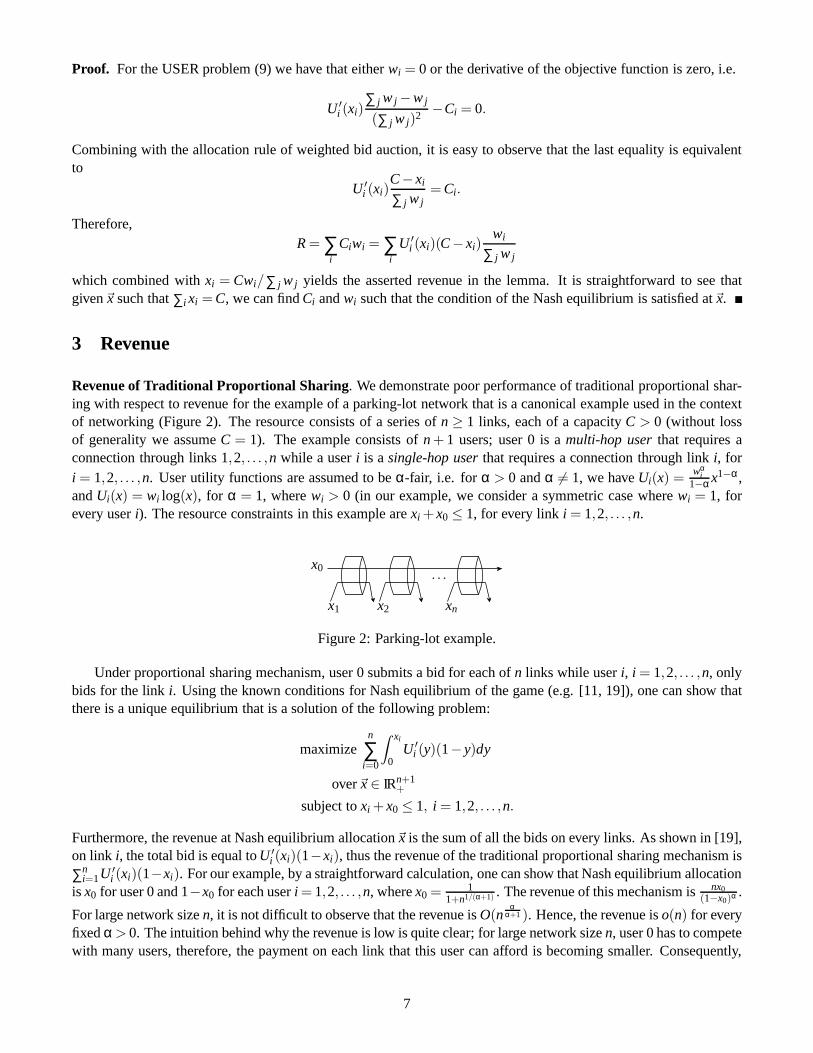
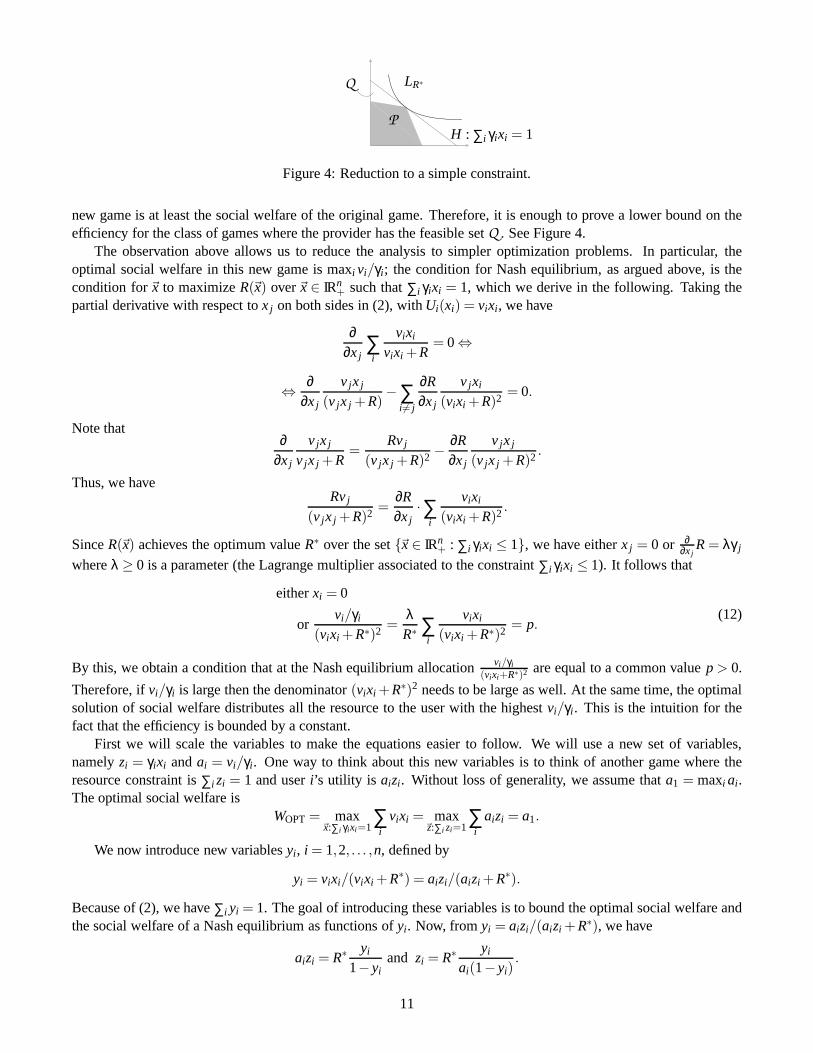
Since for every~x∈ P , R(~x)≤ R∗, the two convex setsLR∗ andP do not have common interior points. LetH bea hyperplane that weakly separates these two sets. This hyperplane can be written as

∑i

γixi = 1, with γi ≥ 0 for eachi. (11)

Consider the game where the provider has the feasible setQ = {~x ∈ IRn+ : ∑i γixi ≤ 1}, then the allocation that

maximizes the revenue overQ is the same as in the original game. SinceP ⊂ Q , the optimal social welfare of the

10

H : ∑i γixi = 1P

Q LR∗

Figure 4: Reduction to a simple constraint.

new game is at least the social welfare of the original game. Therefore, it is enough to prove a lower bound on theefficiency for the class of games where the provider has the feasible setQ . See Figure 4.

The observation above allows us to reduce the analysis to simpler optimization problems. In particular, theoptimal social welfare in this new game is maxi vi/γi ; the condition for Nash equilibrium, as argued above, is thecondition for~x to maximizeR(~x) over~x∈ IRn

+ such that∑i γixi = 1, which we derive in the following. Taking thepartial derivative with respect tox j on both sides in (2), withUi(xi) = vixi , we have

∂∂x j

∑i

vixi

vixi +R= 0⇔

⇔ ∂∂x j

v jx j

(v jx j +R)−∑

i 6= j

∂R∂x j

v jxi

(vixi +R)2 = 0.

Note that∂

∂x j

v jx j

v jx j +R=

Rvj

(v jx j +R)2 −∂R∂x j

v jx j

(v jx j +R)2 .

Thus, we haveRvj

(v jx j +R)2 =∂R∂x j

·∑i

vixi

(vixi +R)2 .

SinceR(~x) achieves the optimum valueR∗ over the set{~x∈ IRn+ : ∑i γixi ≤ 1}, we have eitherx j = 0 or ∂

∂xjR= λγ j

whereλ ≥ 0 is a parameter (the Lagrange multiplier associated to the constraint∑i γixi ≤ 1). It follows that

eitherxi = 0

orvi/γi

(vixi +R∗)2 =λR∗ ∑

i

vixi

(vixi +R∗)2 = p.(12)

By this, we obtain a condition that at the Nash equilibrium allocation vi/γi

(vixi+R∗)2 are equal to a common valuep> 0.

Therefore, ifvi/γi is large then the denominator(vixi +R∗)2 needs to be large as well. At the same time, the optimalsolution of social welfare distributes all the resource to the user with the highestvi/γi . This is the intuition for thefact that the efficiency is bounded by a constant.

First we will scale the variables to make the equations easier to follow. We will use a new set of variables,namelyzi = γixi andai = vi/γi . One way to think about this new variables is to think of another game where theresource constraint is∑i zi = 1 and useri’s utility is aizi . Without loss of generality, we assume thata1 = maxi ai .The optimal social welfare is

WOPT= max~x:∑i γixi=1

∑i

vixi = max~z:∑i zi=1

∑i

aizi = a1.

We now introduce new variablesyi , i = 1,2, . . . ,n, defined by

yi = vixi/(vixi +R∗) = aizi/(aizi +R∗).

Because of (2), we have∑i yi = 1. The goal of introducing these variables is to bound the optimal social welfare andthe social welfare of a Nash equilibrium as functions ofyi . Now, fromyi = aizi/(aizi +R∗), we have

aizi = R∗ yi

1−yiand zi = R∗ yi

ai(1−yi).

11

Next, we are going to bound the social welfare of a Nash equilibrium and the optimal solution.The social welfare at the Nash equilibrium, which we denote asWNASH, can be bounded using the relations above

as follows

WNASH = ∑i

aizi = R∗∑i

yi

1−yi

≥ R∗(

y1

1−y1+∑

i≥2

yi

)

= R∗(

y1

1−y1+1−y1

)

≥ R∗ y21−y1+11−y1

. (13)

The above inequality uses the fact thatyi1−yi

≥ yi and∑i yi = 1.On the other hand, the optimal social welfare, as argued above, is

WOPT= maxi

ai = a1.

To bounda1 as a function ofyi , we multiplya1 with ∑i zi , which is 1, and use the relation betweenzi andyi to haveWOPT as a function ofyi . Specifically,

WOPT= a1 = a1

(

∑i

zi

)

= a1R∗∑i

yi

ai(1−yi). (14)

Now, we use the condition for Nash equilibrium. (Note that this is the only place in the proof that uses (12).) Firstwe rewrite the condition for the variableszi andai . Replacingai = vi/γi andvixi = aizi = R∗ yi

1−yiin to the condition

for Nash equilibrium (12), we can derive

eitheryi = 0 orai(1−yi)

2

R∗2 = p> 0.

From this condition, we haveai(1−yi)2 = a1(1−y1)

2 whenevery1,yi > 0, henceai(1−yi) =a1(1−y1)

2

1−yi. Replacing

this equality in the optimal social welfare (14), we have

WOPT= a1R∗∑i

yi

ai(1−yi)=

R∗

(1−y1)2 ∑i

yi(1−yi)

≤ R∗

(1−y1)2

(

y1(1−y1)+∑i≥2

yi

)

.

The last inequality uses the fact thatyi(1−yi)≤ yi . Using this and replacing∑i≥2 yi = 1−y1, we obtain

WOPT≤R∗

(1−y1)2 (y1(1−y1)+1−y1) = R∗ 1−y21

(1−y1)2 . (15)

From (13) and (15), we have the following lower bound for the efficiency

WNASH

WOPT≥ y2

1−y1+1y1+1

.

By a simple calculus, one can show that the right-hand side isat least 1/(1+2/√

3), which is what we needed toprove.

12

4.2 Efficiency of Weighted Payment Auction

For weighted payment auction, we establish the following result.

Theorem 3 Assuming that the provider maximizes the revenue, the efficiency is bounded by 1/2 for weighted pay-ment auction, and this bound is tight.

Proof. The revenueR(~x) at the Nash equilibrium allocation~x of the weighted payment auction is given by Lemma 2.Therefore,R(x) is maximized over~x∈ IRn

+ subject to the constraint∑i xi =C, when

ddxi

(

U ′i (xi)xi(1−

xi

C))

= λ > 0 wheneverxi > 0.

In the case of linear utility functions,Ui(xi) = vixi , this means

vi

(

1−2xi

C

)

= λ > 0 wheneverxi > 0.

We assume thatv1 ≥ v2 ≥ ·· · ≥ vn. From the condition above, one has:

if xi > 0, thenvi =λ

1−2xiC

> λ = v1

(

1−2x1

C

)

.

Therefore, the social welfare at Nash equilibrium allocation~x is ∑i vixi , and is at least

v1x1+v1

(

1−2x1

C

)

(

n

∑i=2

xi

)

= v1x1+v1

(

1−2x1

C

)

(C−x1).

By a straightforward calculation, one can see that comparedwith the optimal social welfare, which isCv1, the valueabove is at least 1/2 of the optimal social welfare.

The bound can be achieved, for example, forv1 = 1 andv2 = v3 = · · ·= vn =1n asn goes to infinity.

5 Extension to Multiple Providers and General User Utilities

In this section, we will extend the efficiency result of the previous section to the case of multiple competing providersand a broad class of utility functions. Our main result in this section shows a surprising fact that even in complexcompetitive environments, the efficiency can be bounded by aconstant independent of the number of providers andusers (Theorem 4). We first define the framework for multiple providers.

5.1 Multiple Providers

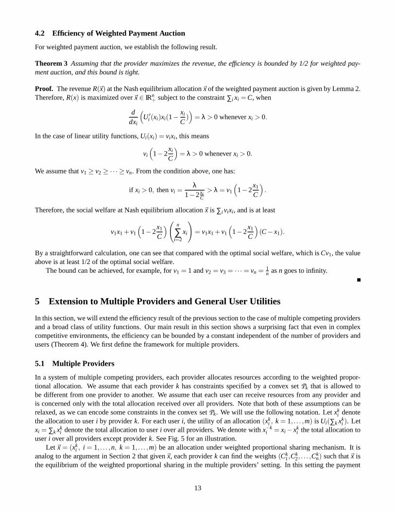
In a system of multiple competing providers, each provider allocates resources according to the weighted propor-tional allocation. We assume that each providerk has constraints specified by a convex setPk that is allowed tobe different from one provider to another. We assume that each user can receive resources from any provider andis concerned only with the total allocation received over all providers. Note that both of these assumptions can berelaxed, as we can encode some constraints in the convex setPk. We will use the following notation. Letxk

i denotethe allocation to useri by providerk. For each useri, the utility of an allocation(xk

i , k= 1, . . . ,m) is Ui(∑k xki ). Let

xi = ∑k xki denote the total allocation to useri over all providers. We denote withx−k

i = xi −xki the total allocation to

useri over all providers except providerk. See Fig. 5 for an illustration.Let~x= (xk

i , i = 1, . . . ,n, k = 1, . . . ,m) be an allocation under weighted proportional sharing mechanism. It isanalog to the argument in Section 2 that given~x, each providerk can find the weights(Ck

1,Ck2, . . . ,C

kn) such that~x is

the equilibrium of the weighted proportional sharing in themultiple providers’ setting. In this setting the payment

13

1 2 providerk m

1 2 useri n

xki

Figure 5: The setting of multiple providers competing in offering resources to users.

of useri to providerk is wki , and the user’s goal is to maximizeUi(∑k xk

i )−∑k wki , wherexk

i = Cki wk

i /∑i wki . The

providerk, on the other hand, obtains the revenueRk, which satisfies the following

n

∑i=1

U ′i (x

−ki +xk

i )xki

U ′i (x

−ki +xk

i )xki +Rk

= 1. (16)

In order to gain some intuition, note that if for everyi, Ui(x) is a concave function, thenU ′i (x

−ki +xk

i ) decreaseswith x−k

i . From this, we can see that the marginal utility for a user with a providerk decreases if the user alreadyreceived allocations from other providers. As a result, provider k may extract smaller revenue due to competitionwith other providers. With this in mind, we now define an equilibrium in the case of multiple providers.

Definition 1 We call~x an equilibrium allocation if for every k, the allocation vector~xk = (xk1, . . . ,x

kn) maximizes Rk

given by (16) over the setPk.

We note that in the multiple providers setting, we can think of the game as the providerk’s strategy set isPk. Thediscrimination weights and the revenue then can be calculated according to the allocation vector~x of all providers.With these discrimination weights, under users’ selfish behavior ~x will be an outcome of the game. From theproviders’ perspective, an equilibrium allocation is an allocation~x where no provider has an incentive to unilaterallychange its allocation vector. Note that when there is only one provider, this game is the same as the two-stageStackelberg game considered in Section 2.

5.2 A Class of Utility Functions

We introduce a class of utility functions defined as follows.

Definition 2 Let U(x) be a non-negative, increasing, and concave utility function and let x0 ≥ 0 be the value max-imizing U′(x)x. We call U(x), δ-utility, if, in addition, the following two conditions hold: (i) U ′(x)x is a concavefunction over[0,x0], and (ii) there existsδ ∈ [0,∞), such that, for every a∈ [0,x0],

U(b)− [U ′(a)a]′b≤ δU(a)

where b is such that U′(b) = [U ′(a)a]′ =U ′(a)+U ′′(a)a≥ 0.

In Figure 6, we show geometric interpretations of the latterdefinition.While the definition may appear somewhat technical, in fact,it has strong connections with the theory of third-

degree price discrimination [24], which we discuss in Appendix D. Furthermore, the class accommodates manyutility functions commonly considered in literature. Specifically, we can show that a linear function or a truncatedlinear function is 0-utility, a polynomialU(x) = (c+x)α for c≥ 0 is a e

2-utility for any 0≤ α ≤ 1, or a logarithmicfunction is a 2-utility; we provide a detailed list and proofs in Appendix E. We briefly comment that truncatedlinear utility functions or logarithmic functions were considered representative of real-time traffic requirementsin communication networks [23], concave marginal utilities were considered in [20], polynomial utility functionswere used in many models of economics [24],α-fair utility functions [14] were widely used in the contextofcommunication network resource sharing and a class of utility functions that characterize TCP-like connections [12].Finally, we note the following result whose proof is available Appendix B.1.

14

PSfrag

x xa ab b

U ′(x)U(x)

[U ′(x)x]′ =U ′(x)+U ′′(x)xWWL

L

slopeU ′(b) =U ′(a)+U ′′(a)a

Figure 6: LW ≤ δ where (left)L andW are lengths of the line segments and (right)L is the shaded andW is the hatched area.

Lemma 4 If f and g areδ-utilities, then so are: c· f , for c> 0; truncation of f with a positive number; and f+g.

As a consequence, every polynomial of the form∑i aixαi whereai > 0 and 0≤ αi ≤ 1 is a e2-utility function.

5.3 Efficiency Bound

We now state and prove our main theorem on the efficiency of weighted bid auctions.

Theorem 4 Assume that for every user i and every a≥ 0, U ′i (x+a)x is a continuous and concave function. Then,

there exists an equilibrium in the case of multiple providers defined as above. Furthermore if Ui(a+x) areδ-utilities,then the efficiency at any equilibrium is at least1/(1+2/

√3+δ).

Note that when the utility functions are linear, i.e.δ = 0, we have Theorem 2 as a special case. The result ofTheorem 4 is rather surprising as it is not a priori clear thatin a complex system where both users and providers aimat selfishly maximizing their individual payoffs (objectives which often conflict each other), the efficiency would bebounded by a constant that is independent of the number of users and the number of providers.

Before going into the proof of Theorem 4 provided below, we briefly describe the main ideas. The key idea of theproof is to bound the social welfare of the system, which is a complicated optimization problem over the Minkowskisum of the setsPk, where the resource setPk of the providerk can be different. If the utility functions are linear,then this optimization problem can beseparatedinto a collection of optimization problems over each setPk, andthe optimal value is the sum of these optimal values. Using this idea, we will bound the utility function by an affinefunction that is a tangent to the concave utility at the pointdefined by the value at the Nash equilibrium. This idea isillustrated in Figure 7. It will be shown that because of the property ofδ-utilities, the valueai in the figure is at mostδUi(xi), which will be a key inequality of the proof.2

ai

xi yi

Ui(x)

Vi(x)

Figure 7: The key bounding ofUi(x) with the affine functionVi(x) such thatV ′i (yi) =U ′

i (xi)+U ′′i (xi)maxk xk

i andVi(yi) =Ui(yi).

2We note that our proof technique is rather general and that a similar result for weighted payment auctions can also be obtained usingthis framework. However, we omit to provide details as our focus is on weighted bid auctions that allow for much more general resourceconstraints.

15

Proof. The proof for the first part of the theorem about the existenceof a Nash equilibrium uses standard fixed pointtheorem argument. A formal proof is given in Appendix refapp:fix.

For the second part, the key idea of the proof is to bound the social welfare by an affine function which allowsseparating the maximization over(~x1, . . . ,~xm) ∈ ∑k Pk to maximizations over the setsPk, where∑k Pk := {~z1+ · · ·+~zm : ~zk ∈ Pk,k= 1, . . . ,m} is the Minkowski sum of the setsPk. Once the optimization problem is separated, we canuse a similar bound as in Section 4 ( see Lemma 5 below) as a subroutine to prove the theorem. Now, let

vki =U ′

i (xi)+U ′′i (xi)x

ki , for eachi, andvi = min

kvk

i .

Since for everyi, Ui(x) is a concave function,U ′′i (x) is non-positive, and thus,

vi =U ′i (xi)+U ′′

i (xi)(maxk

xki )≥U ′

i (xi)+U ′′i (xi)xi .

The last inequality is because of the factxi = ∑k xki .

Now, let us defineVi(x) = ai + vix whereai is chosen so thatVi(x) is a tangent toUi(x). Let yi be the point atwhich the functionsVi(x) andUi(x) intersect. We will useVi(x) as an upper bound ofUi(x) for everyx≥ 0. We haveai =Ui(yi)− (U ′

i (xi)+U ′′i (xi)xi)yi . By the definition ofδ-utility functions,ai ≤ δUi(xi).

Therefore,

∑i

ai ≤ δ∑i

Ui(xi). (17)

SinceUi(x) is a non-negative concave function, we haveUi(x)≤Vi(x). Hence,

max~z∈∑k Pk

∑i

Ui(zi) ≤ max~z∈∑k Pk

∑i

Vi(zi)

= ∑i

ai + max~z∈∑k Pk

∑i

vizi

= ∑i

ai +∑k

max~z∈Pk

∑i

vizi . (18)

The last is the key inequality as it enables us to use the fact that vizi are linear functions, therefore, instead ofconsidering the maximization over the set∑k Pk we can bound∑i vizi over eachPk.

By similar arguments as in the proof of Theorem 2, we can provethe following lemma whose proof is providedin Appendix B.3.

Lemma 5 For ever k,

∑i

U ′i (xi)x

ki ≥

1

1+2/√

3maxz∈Pk

∑i

vki zi . (19)

We now use this lemma to prove our main result. On the one hand,if we sum the left-hand side of (19) over allk,we have

∑k,i

U ′i (xi)x

ki = ∑

i

U ′i (xi)xi ≤ ∑

i

Ui(xi) (20)

where the last inequality is true becauseUi(x) is a non-negative and concave function for everyi. On the other hand,if we sum the right-hand side of (19) over allk, we obtain

∑k

1

1+2/√

3maxz∈Pk

∑i

vki zi ≥

1

1+2/√

3∑k

maxz∈Pk

∑i

vizi (21)

where in the last inequality,vki are replaced byvi , which recall is equal to mink vk

i .Combining (19)–(21), we derive

∑i

Ui(xi)≥1

1+2/√

3∑k

maxz∈Pk

∑i

vizi

16

⇒ (1+2/√

3)∑i

Ui(xi)≥ ∑k

maxz∈Pk

∑i

vizi . (22)

Finally, from (17), (18) and (22), we have

max~z∈∑k Pk

∑i

Ui(zi)≤ (δ+1+2/√

3)∑i

Ui(xi)

which establishes the asserted result.

6 Convergence and Distributed Algorithms

In this section we demonstrate how a provider may adjust userdiscrimination weights by an iterative algorithmwhose limit points are Nash equilibrium points of the resource competition game that we studied in earlier sections.We focus on weighted bid auctions but note that similar type of analysis can be carried out for weighted paymentauctions. Our aim in this section is to show how such iterative algorithms can be designed in principle.3

One of the main ideas is to relax polyhedron constraints by introducing apenaltyfunction P(~x) that is chosenso that to confine the allocation vector~x within the feasible set specified by our polyhedron constraints A~x ≤~b.Intuitively, function P(~x) would be chosen to assume small values for every feasible allocation vector~x that issufficiently away from the boundary of the feasible set and would grow large as the allocation vector~x approaches theboundary of the feasible set. We assume thatP(~x) is continuously differentiable and convex function. Specifically,we assume that for a collection of functionsPl , one for each of the constraints, we have

P(~x) =∑l

Pl

(

∑j

al , j x j

)

.

Indeed, ifPl is continuously differentiable and convex function for every l , then so isP. We defineV(~x)=R(~x)−P(~x)whereR(~x) is the revenue given by (2). The provider’s problem is redefined to

PROVIDER ′ : maximizeV(~x) over~x∈ IRn+.

In the remainder of this section, we first show how the provider would adjust discrimination weights assumingthat the provider knows user utility functions and establish convergence to the Nash equilibrium points in this case.This provides a baseline dynamics that we then approximate as follows. We consider a provider who a prioridoes not know user utility functions but estimates the needed information in an online fashion while adjustingthe discrimination weights. The main idea here is to use an argument based onseparation of timescaleswherediscrimination weights are adjusted by the provider at a slower timescale in comparison with the rate at which bidsare received from users, allowing the provider to estimate the needed information about the user utility functions forevery given set of discrimination weights. We will formulate iterative algorithms as dynamical systems in continuoustime as this is standard in previous work, e.g. [13], and it readily suggests practical distributed algorithms.

User Utility Functions a Priori Known . Suppose that user utility functions are a priori known by the provider(this may be the case if profiles of users are known to the provider, e.g. from the history of previous interactions).The provider announces discrimination weights~C(t) at every timet ≥ 0 that are adjusted as follows. The providercomputes the allocation vector~x(t) according to the following system of ordinary differentialequations, for someα > 0,

ddt

xi(t) = αxi(t)∂

∂xiV(~x(t)), i = 1,2, . . . ,n. (23)

For every timet ≥ 0, the provider announces to users the discrimination weights ~C(t) where the discriminationweight for useri is:

Ci(t) = xi(t)+R(~x(t))

U ′i (xi(t))

.

3Note that it is beyond the scope of this paper to fully specifysome of the implementation details such as online estimation of the elasticityof user utility functions and address the stability in presence of feedback delays.

17

Notice that the right-hand side in the system (23) requires knowledge of the gradient of the revenue functionR(~x),which is given by

∂∂xi

R(~x) = φ(~x)[U ′

i (xi)xi ]′

(U ′i (xi)xi +R(~x))2 (24)

where

φ(~x) =R(~x)

∑ jU ′

j (xj )xj

(U ′j (xj )xj+R(~x))2

.

The convergence to optimal solution of PROVIDER’ is showed in the following result.

Theorem 5 Suppose that for every user i, U′i (x)x is continuously differentiable and concave function and that P(~x)is a strictly convex function. Then, every trajectory(~x(t), t ≥ 0) of the system (23) converges to a unique maximizerof the function V(~x).

The proof is based on standard application of Lyapunov stability theorem and is thus omitted here. It amountsto showing that the functionV is a Lyapunov function for the system (23) that increases along every trajectory~x(t),thus implying convergence to the unique maximizer ofV.

User Utility Functions a Priori Unknown . We now discuss how the user discrimination weights would beadjustedby a provider who does not a priori know the user utility functions. The key idea is to use aseparation of timescales:the provider adjusts the discrimination weights at a slowertimescale than the timescale at which bids are adjusted byusers. Informally speaking, this allows the provider to actas if for every fixed set of discrimination weights, usersadjust their bids instantly to Nash equilibrium bids.

From (6) and the allocation rulexi =Ciwi/∑ j w j one readily observes that the following identities hold at Nashequilibrium:

U ′i (xi)xi =

Rwi

R−wiandU ′

i (xi)xi +R=R2

R−wi

whereR= ∑ j w j . Using these identities, we observe that the gradient in (24) can be expressed as follows

∂∂xi

R= RwiR

(

1− wiR

)

1xi+(

1− wiR

)2 U ′′i (xi)xi

R

∑ jwj

R

(

1− wj

R

) . (25)

Notice that the gradient is fully expressed as a function of the vector of user bids~w except for the term that involvesthe second derivative of the user utility function. For the case of linear user utility functions, we haveU ′′

i (xi) = 0 foreveryi, and thus, in this case the gradient of the revenueR(~x) is fully described by the vector of bids~w.

In general, we assume that at every timet ≥ 0, the provider sets the user discrimination weight for useri asfollows

Ci(t) =R(~w(t))

wi(t)xi(t).

For the case of linear utility function,~x(t) is assumed to evolve according to the following system of ordinarydifferential equations, for someα > 0, and everyi = 1,2, . . . ,n,

ddt

xi(t) = α [vi(wi(t),R(~w(t)))−xi(t)pi(~x(t))] (26)

where

vi(wi,R) = RwiR

(

1− wiR

)

∑ jwj

R

(

1− wj

R

)

pi(~x) = ∑l

al ,iP′l

(

∑j

al , j x j(t)

)

.

18

In general, each useri is assumed to adjusts its bidwi(t) using the following natural dynamics for solving hisUSER problem:

ddt

wi(t) =U ′i (xi(t))xi(t)−R(~w(t))

wi(t)R(~w(t))

1− wi (t)R(~w(t))

. (27)

The following result establishes convergence for the case of linear user utility functions, which are a prioriunknown by the provider.

Theorem 6 Suppose that user utility functions are linear. For every sufficiently smallα > 0, the allocation vectorunder system (26)-(27) approximates that of the system (23)with an approximation error diminishing withα.

We note that this proof is based on applying theaveraging theoryof non-linear dynamical systems [16]. Itestablishes global asymptotic stability of the system (27)for the allocation vector~x(t) fixed to an arbitrary feasibleallocation vector~x for everyt ≥ 0, which is of independent interest as it applies also for non-linear utility functions.

Proof. We first assume that~x(t) is fixed to an arbitrary feasible allocation~x, for everyt ≥ 0, and then establishglobal asymptotic stability of the system (27), i.e. that every trajectory~w(t) converges to a unique limit point. Letus use the notationai =U ′

i (xi)xi , for everyi. Let L : IRn+ → IR be the function defined as follows

L(~w) =n

∑j=1

log(w j)− log(n

∑j=1

w j)−n

∑j=1

w j

a j.

We show that for every trajectory~w(t) of the system (27), we haveddt L(~w(t))≥ 0, for everyt ≥ 0. Indeed,

ddt

L(~w) =n

∑i=1

∂wi

L(~w)ddt

wi =n

∑i=1

1ai

(

1wi

− 1

∑nj=1w j

)(

ai −wi

1− wi∑n

j=1 wj

)2

which is non-negative for every~w ∈ IRn+. Now, for the system (27) there exists (a positive invariantset)S that is

compact and such that if~w(0) ∈ S, then~w(t) ∈ S, for everyt ≥ 0. For example, it is not difficult to establish that onesuch set isS= [0,w]n, wherew= maxi{max{vi ,wi(0)}}. By LaSalle’s theorem(e.g. Theorem 4.4 [16]) we havethat every solution~w(t) started inSconverges to the maximizer of the functionL(~w), which is unique and given bywi = Rai/(ai +R) whereR is such that∑i ai/(ai +R) = 1.

Having established the above convergence, it is not difficult to observe that for everyi,

limT→∞

1T

∫ T

0[ui(t)−xi pi(~x)]dt = xi

∂∂xi

V(~x)

and∣

∣

∣

∣

∣

∣

∣

∣

1T

∫ T

0[ui(t)−xi pi(~x)]dt−xi

∂∂xi

V(~x)

∣

∣

∣

∣

∣

∣

∣

∣

≤ c(T)

whereui(t) := vi(wi(t),R(~w(t))) andc is a strictly decreasing, continuous, and bounded functionthat converges tozero asT goes to infinity.

Finally, let~x(t), for t ≥ 0, be the solution of the system(d/dt)xi(t) = xi(t) ∂∂xi

V(~x(t)). Then, by theaveraging

theoremTheorem 10.5 [16], we have that if~x(αt) is within the domain for every 0≤ t ≤ b/α and~x(0)−~x(0) ∈O(c(α)), then for every sufficiently smallα > 0, we have~x(t)−~x(αt) = O(c(α)), for every 0≤ t ≤ b/α. Thisshows that the solution of the averaged dynamics of the system (26)-(27) approximates that of the system (23) andcompletes the proof.

Same approach applies more generally for non-linear user utility functions but one would need to use an onlineestimator of the second derivative of the utility function in (25) from the observed bids submitted by users.4 In

4Notice that the need to infer these second derivatives of theutility functions is not an artifact of the auction scheme that we use, but isintrinsic to any revenue maximization problem.

19

0 50 1000

0.5

1

t

x i(t)/

(x0(t

)+x i(t

))single−hop user

multi−hop user

0 50 1000

0.5

1

t

x i(t)/

(x0(t

)+x i(t

))

single−hop user

multi−hop user

Figure 8: Convergence to equilibrium points for the parking-lot example: (Left) a priori known utility functions and(Right) a priori unknown utility functions.

0 50 1000

0.5

1

t

x i(t)/

(x0(t

)+x i(t

))

single−hop user

multi−hop user

0 50 1000

0.5

1

t

x i(t)/

(x0(t

)+x i(t

))

single−hop user

multi−hop user

Figure 9: Another example for the convergence to equilibrium points for the parking-lot: (Left) a priori known utilityfunctions and (Right) a priori unknown utility functions.

principle, this can be done by observing the effect of perturbing the allocation for a user on the bid submitted bythis user, which we briefly discuss in the following. From (6)and the allocation rulexi = Ciwi/∑ j w j , we haveU ′

i (xi) =Rxi

wiR/(1−

wiR ). Taking the derivative with respect toxi, we obtain

U ′′i (xi)xi =

wiR

1− wiR

(

∂∂xi

R− 1xi

R

)

+R1

(

1− wiR

)2

∂∂xi

(wi

R

)

.

Plugging this in (25), we have

∂∂xi

R=R

∑ jwj

R

(

1− wj

R

)

− wiR

(

1− wiR

)

∂∂xi

(wi

R

)

.

Therefore, the gradient of the revenue can be fully expressed in terms of the bids~w and the terms(∂/∂xi)(wi/R),which can be estimated in an online fashion by perturbing theallocation of useri and observing the resulting changeof wi/R.

Parking-Lot Example. We demonstrate convergence of the iterative scheme (26)-(27) for the example of parking-lot network which we introduced in Section 3 (Figure 2). Recall that the resource consists ofn≥ 1 links, each ofcapacity 1, with a multi-hop user 0 with allocationx0 at each link and a single-hop user with allocationxi at eachlink i. User utility functions are assumed to be linearUi(x) = vix, for x≥ 0, wherevi = v1, for i = 1,2, . . . ,n, andv0,v1 > 0.

The Nash equilibrium allocation and the corresponding revenue are specified in the following lemma whoseproof is simple and thus omitted.

20

Lemma 6 Let η = n−12√

n

√

v1v0

. For the parking-lot scenario, the Nash equilibrium allocation is 1−x1 for user0 and

x1 for each user i= 1,2, . . . ,n, where

x1 =

{

12(1−η) , for η < 1/2

1, for η ≥ 1/2. (28)

The revenue at the Nash equilibrium is given by

R=

{

14η(1−η)(n−1)v1, for η < 1/2

(n−1)v1, for η ≥ 1/2.

We note that the Nash equilibrium allocation to a single-hopuser is increasing with the ratio of the valuationsv1/v0, from 1/2 for v1/v0 = 0 to 1 forv1/v0 = n/(n−1)2 and beyond this at each link the single-hop user is allocatedthe entire link capacity.

In the remainder of this section we illustrate convergence for two particular cases. In either case we considerthe case withn= 5 links and linear utility functions specified byv0 = 5 andv1 = v2 = · · · = vn = 1. The link costfunctions are defined as

P′l (x) =

{

0, 0≤ x≤ ρ0,(

1x − 1

1−ρ0

)p, ρ0 < x≤ 1

where p > 0 and in particular we usep = 2 andρ0 = 0.8. We show results for initial allocation~x(0) such thatx1(0) = x2(0) = · · ·= xn(0), so that due to symmetryx1(t) = x2(t) = · · ·= xn(t), for everyt ≥ 0. This simplifies theexposition. Indeed, we validated convergence for various other initial values other choices of other parameters butfor space reasons confine to the above asserted setting.

We first demonstrate convergence for a closed system with a fixed set of users. In Figure 8 we show trajectoriesfor the allocationsx0(t) andx1(t) for both a priori known utility functions (left) and a prioriunknown utility functions(right), with α set to 0.1. The results indeed validate convergence to the Nash equilibrium allocation, which areindicated with dashed lines. Our other example consists of an open system where at a specific timet1 ≥ 0 a single-hop user departs the system and then another such user arrives at timet2 > t1. In particular, we use the valuest1 = 30,t2 = 70, andα = 0.8. Figure 8 well validates convergence to the Nash equilibrium allocation in this case.

7 Conclusion

We considered a simple mechanism for allocation of a resource owned by a provider to users that allows for discrim-ination of users and general resource constraints specifiedby convex polyhedrons, thus allowing for provisioningof a variety of systems and services. We showed that in a competitive framework where everyone is selfish, in awide set of cases, the mechanism guarantees nearly optimal revenue to the provider and competitive social efficiency(including a setting with multiple providers). Besides analysis of equilibrium points of the underlying competitiongame, we also showed how one would design an iterative algorithm that converges to the equilibrium points.

The work suggests several interesting directions for future research. First, it would be of interest to study revenueand efficiency properties for classes of user utility functions that are not accommodated by our framework, e.g.other thanδ-utility functions. Second, it would also be of interest to purse a more in-depth analysis of convergenceproperties of the algorithms in this paper; in particular, it would be of interest to consider implementation details andaddress the stability properties of the underlying schemes.

References

[1] Amazon Web Services. Amazon EC2 Spot Instances. http://aws.amazon.com/ec2/spot-instances, 2010.

21

[2] A. Demers, S. Keshav, and S. Shenker. Analysis and simulation of a fair queueing algorithm.Internetworking:Research and Experience, 1:3–26, 1990.

[3] B. Edelman, M. Ostrovsky, and M. Schwartz. Internet advertising and the generalized second price auction:Selling billions of dollars worth of keywords.American Economic Review, 97(1):242–259, 2007.

[4] M. Feldman, K. Lai, and L. Zhang. A price-anticipating resource allocation mechanism for distributed sharedclusters. InProc. of ACM EC, 2005.

[5] R. J. Gibbens and F. P. Kelly. On packet marking at priority queues. IEEE Trans. on Automatic Control,47:1016–1020, 2002.

[6] D. K. Golldenberg, L. Qiuy, H. Xie, Y. R. Yang, and Y. Zhang. Optimizing cost and performance for multi-homing. InProc. of ACM Sigcomm’04, Portland, Oregon, USA, 2004.

[7] A. Gulati, I. Ahmad, and C. A. Waldspurger. Parda: proportional allocation of resources for distributed access.In Proc. of FAST’09, San Francisco, CA, 2009.

[8] B. Hajek and S. Yang. Strategic buyers in a sum bid game forflat networks. InIMA Workshop, March 2004.

[9] J. Hartline and A. Karlin.Algorithmic Game Theory, chapter Profit Maximization in Mechanism Design, pages331–362. editors N. Nisan, T. Roughgarden, E. Tardos, and V.V. Vazirani, Cambridge University Press, 2007.

[10] L. He and J. Walrand. Pricing and revenue sharing strategies for internet service providers.IEEE/ACM Journalon Selected Areas in Comm., 24(5):942–951, 2006.

[11] R. Johari and J. N. Tsitsiklis. Efficiency loss in a network resource allocation game.Mathematics of OperationsResearch, 29(3):402–435, 2004.

[12] F. Kelly. Mathematics Unlimited - 2001 and Beyond, chapter Mathematical modelling of the Internet, pages685–702. editors B. Engquist and W. Schmid. Springer-Verlag, Berlin, 2001.

[13] F. P. Kelly. Charging and rate control for elastic traffic. European Trans. on Telecommunications, 8:33–37,1997.

[14] F. P. Kelly, A. K. Maulloo, and D. K. H. Tan. Rate control for communication networks: Shadow prices,proportional fairness and stability.Journal of the Operational Research Society, 49, 1998.

[15] P. Key, L. Massoulie, and M. Vojnovic. Farsighted users harness network time-diversity. InProc. of IEEEInfocom 2005, Miami, FL, USA, 2005.

[16] H. K. Khalil. Nonlinear Systems. Prentice Hall, 3 edition, 2001.

[17] S. Lagaie, D. M. P. A. Saberi, and R. V. Vohra.Algorithmic Game Theory, chapter Sponsored Search Auctions,pages 699–716. editors N. Nisan, T. Roughgarden, E. Tardos,and V. V. Vazirani, Cambridge University Press,2007.

[18] R. T. Ma, D. M. Chiu, J. C. S. Lui, V. Misra, and D. Rubenstein. On resource management for cloud users: Ageneralized kelly mechanism approach. Technical report, Technical Report, Electrical Engineering, May 2010.

[19] T. Nguyen and E. Tardos. Approximately maximizing efficiency and revenue in polyhedral environments. InProc. of ACM EC’07, pages 11–19, 2007.

[20] A. Ozdaglar and R. Srikant.Algorithmic Game Theory, chapter Incentives and Pricing in CommunicationNetworks. editors N. Nisan, T. Roughgarden, E. Tardos, and V. V. Vazirani, Cambridge University Press, 2007.

[21] A. K. Parekh and R. G. Gallager. A generalized processorsharing approach to flow control in integratedservices networks: The multi node case.IEEE/ACM Trans. on Networking, 2:137–150, April 1994.

22

[22] S. Shakkottai and R. Srikant. Economics of network pricing with multiple isps. IEEE/ACM Trans. on Net-working, 14(6):1233–1245, 2006.

[23] S. Shakottai, R. Srikant, A. Ozdaglar, and D. Acemoglu.The price of simplicity. IEEE Journal on SelectedAreas in Communications, 26(7):1269–1276, 2008.

[24] J. Tirole. The Theory of Industrial Organization. The MIT Press, 2001.

[25] H. R. Varian.Microeconomic Analysis. Norton, 3 edition, 1992.

[26] G. Wang, A. Kowli, M. Negrete-Pincetic, E. Shafieepoorfard, and S. Meyn. A control theorist’s perspectiveon dynamic competitive equilibria in electricity markets.In Proc. 18th World Congress of the InternationalFederation of Automatic Control (IFAC), Milano, Italy, 2011.

[27] Wikipedia. California electricity crises. http://en.wikipedia.org/wiki/California_electricity_crisis, 2010.

A Applications of General Polyhedral Environments

We explain some applications of the resource allocation problem with general polyhedral constraints.

Network bandwidth sharing

The most natural example is the bandwidth sharing game, where each provider owns a network of capacitated links,each useri is sending traffic along a pathPi andxi is the data transfer rate for useri. In this case we have a resourceconstraint associated to each linke: ∑i:e∈Pi

xi ≤ ce wherece is the capacity of linke.

Keyword auctions

The general convex constraints can also capture a general model of keyword auctions. The auction is for a singlekeyword, and there aren advertisers bidding to have their ad appear as a sponsored search result. There are finite setof outcomes, depending on which bidder gets displayed in which position. We describe each of these outcomes as andimensional vector whose coordinates are the expected number of click that the corresponding advertiser gets. Moreprecisely, let~y1, . . . ,~yN be all the possible outcome vectors, and~yk = (yk

1, . . . ,ykn), wherexk

i is the expected number ofclicks that advertiseri receives at outcomek. To think of keyword auctions as a convex resource allocation, we needto allow randomization in the allocation of bidders to positions. Choosing between the deterministic allocations bythe probability distribution~p= (p1, . . . , pN), we have that∑ j p j~y j is the vector whose coordinates correspond to theexpected number of clicks of an advertiser. Now the set of expected allocation vectors obtained this way is exactlythe convex hullconv(~y1, . . . ,~yN) = {~x :~x= ∑ j p j~y j , p j ∈ [0,1] for every j and ∑ j p j = 1}.

In this model, we will assume a natural condition on the externalities of the click-through rates: if we removean ad from a position (by simply showing one fewer ad), the expected number of clicks received by the remainingads does not decrease. Under this assumption, it is not hard to see that the set of all possible randomized allocationvectors, that is the convex hullconv(~y1, . . . ,~yN), can be written as a polyhedron, which is exactly the constraint ofthe problem considered in this paper.

Traditional keyword auctions use an assignment of ads to positions (ordering) that depends on the bids times anindividual weight, and do not use randomization [17, 3]. Furthermore, the most commonly used framework does notcapture the externalities among ads. Our description of theoutcomes associates an arbitrary nonnegative vector ofclick-through rates with each selection of bidders allocated to a positions. Therefore, this allows us to model the mostgeneral type of externalities between the ads shown. Externalities in keyword auctions are natural and important,for example, the valuation of a bidder for being, say, in position 2 depends on what ad is showed in position 1. Forexample, NIKE in position 1 makes position 2 less valuable forsneakerscompared to having an unknown brandname in position 1.

23

To compete the description of the application in sponsored search auctions, we now give a formal definition anda proof about the externalities among advertisers in this applications.

We say that the a resource allocation problem with a feasibleset of allocationsP in IRn+ satisfies theassumption

of non-positive externalitiesif for any allocation~x∈ P , and any coordinatek, there is an allocation~x′ ∈ P such that(1) x′k = 0, and (2)xi = 0 impliesx′i = 0, andx′i ≥ xi for all i 6= k.

Claim 1 The convex hull of some non-negative vectors~y1, . . . ,~yN that satisfy the assumption of non-positive exter-nalities can be written as{~x∈ IRn

+ : Ax≤~b}, for some matrix A and vector~b.

Proof. Let C be the convex hull of~y1, . . . ,~yN. We will show that if these vectors satisfy the assumption ofnon-positive externalities, then for a vector~w∈C, and any vector~v such that 0≤~v≤ ~w is also inC. With this property,it is not difficult to see from basic convex geometry that the setC can be written as a polyhedron.

We prove this property by induction on the number of non-zerocoordinates of~w. The claim is trivial whenwi = 0 for everyi. Consider a vector~w∈C. The setC is the convex hull of~y1, . . . ,~yN, hence there exist non-negativereal numbersα1, . . . ,αN such that∑i αi = 1, andw= ∑i αixi . Let k be the coordinate that minimizes the ratiovi/wi

for wi 6= 0, and letλ denote this ratio. By definition,λ ≤ 1, and thus ifλ = 1, there is nothing to prove. We use thedefinition of non-positive externalities for each~yi to obtain a vector~zi ∈C with zi

k = 0, and letw′ = ∑i αizi . Considerthe vectorλ~w+(1−λ)~w′ ∈C. By definition ofλ, we have the following facts

• ~w′ ∈C;

• ~w′ has more zero coordinates than~w (namely thekth coordinate);

• thekth coordinate ofλ~w+(1−λ)~w′ is equal tovk;

• λ~w+(1−λ)~w′ ≥~v (as~w′j ≥ ~w j for all coordinatesj 6= k);

• λ~w≤~v which follows asλ was the minimum ratio mini vi/wi .

The last two properties guarantee that there is a vector 0≤~v′ ≤ ~w′ such thatλ~w+(1−λ)~v′ =~v. Now, we use theinduction hypothesis to~w′ ∈C and 0≤~v′ ≤ ~w′ to show that~v′ ∈C, and hence,~v= λ~w+(1−λ)~w′ ∈C.

Scheduling jobs in data centers

This is a problem of allocating data center resources to users. In this application, typically each user needs to finisha job which requires reading many different blocks of data across machines in a data center. LetD j

i be the amountof data of typej that jobi needs to process. The utility function of each jobi is related to its finishing timeti , whichis the maximum processing time of the job across all types of data that it requests. Equivalently, one can model thateach jobi tries to maximize the utilityUi(xi), wherexi = 1/ti . In other words,xi is the minimum amongD j

i /sji ,

wheresji is the speed that jobi can process data of typej. Typically, data centers are complex systems consisting

of many clusters of machines and data has many copies across the clusters. The constraints onsji are complex, but

in many cases it can be captured by convex constraints. Therefore, the allocation vector~x can also be captured byconvex constraints. In this example, it is unrealistic to design a mechanism that requires every job to know exactlythe complex constraints on~x. Simple mechanisms are crucial in these applications.

B Missing Proofs

B.1 Proof of Lemma 4

Items (i) and (ii) are straightforward to show. In the following, we show item (iii).Let h= f +g. Givena≥ 0, letb≥ 0 be such that

[h′(a)a]′ = h′(b). (29)

24

We need to show thath(b)−h′(b)b≤ δh(a)

which corresponds tof (b)− f ′(b)b+g(b)−g′(b)b≤ δ( f (a)+g(a)). (30)

Let b1 andb2 be such that

[ f ′(a)a]′ = f ′(b1) (31)

[g′(a)a]′ = g′(b2) (32)

and, without loss of generality, assumeb1 ≤ b2.Since f andg areδ-utilities, the following two relations hold

f (b1)− f ′(b1)b1 ≤ δ f (a)

g(b2)−g′(b2)b2 ≤ δg(a).

Hence,f (b1)− f ′(b1)b1+g(b2)−g′(b2)b2 ≤ δ( f (a)+g(a)). (33)

In view of (30) and (33), it suffices to show that

f (b)− f ′(b)b+g(b)−g′(b)b≤ f (b1)− f ′(b1)b1+g(b2)−g′(b2)b2. (34)

Note that[h′(a)a]′ = [ f ′(a)a]′+[g′(a)a]′. Combining with (29), (31), and (32), we observe

f ′(b1)+g′(b2) = f ′(b)+g′(b).

Using this identity it is not difficult to conclude thatb1 ≤ b≤ b2 and that we can rewrite (34) as

f (b)− f ′(b1)b+g(b)−g′(b2)b≤ f (b1)− f ′(b1)b1+g(b2)−g′(b2)b2.

The latter inequality indeed holds if the following two inequalities hold

f (b)− f (b1) ≤ f ′(b1)(b−b1)

g(b2)−g(b) ≥ g′(b2)(b2−b)

but the latter two inequalities are indeed true asb1 ≤ b≤ b2 and bothf andg are concave functions.

B.2 Proof of the first part of Theorem 4

For both price taking users and price anticipating users, a Nash equilibrium is determined by a set of allocationvectors(~x1, . . . ,~xm) ∈ P1×·· ·×Pm. Consider the conventional best-response function

F : P1×·· ·×Pm → P1×·· ·×Pm

such that(~y1, . . . ,~ym) = F(~x1, . . . ,~xm), where~yk is the allocation vector that maximizes the revenue for provider k,assuming other providers do not change their allocations. This mapping is continuous and thus by the fixed-pointtheorem, there exists an allocation vector where no provider k can increase his revenue by changing the allocationvector~xk, which is a Nash equilibrium.

25

B.3 Proof of Lemma 5

By similar argument as in the proof of Theorem 2, we can assumethat the convex setPk is of the form

∑i

γixki = 1, with γi ≥ 0 for eachi,

and we can derive the condition, for somep> 0,

eitherxi = 0

or1γi[U ′

i (xi)xki ]′

(U ′i (xi)xk

i +Rk)2=

1γi

vki

(U ′i (xi)xk

i +Rk)2= p. (35)

Let us use the following notation, for each useri,

ai =vk

i

γiandyi =

U ′i (xi)xk

i

U ′i (xi)xk

i +Rk. (36)

Without loss of generality, we assume thata1 ≥ a2 ≥ ·· · ≥ an. From(36), we have

∑i

U ′i (xi)x

ki = Rk∑

i

yi

1−yi≥ Rk

(

y1

1−y1+∑

i≥2

yi

)

=

Rk(

y1

1−y1+(1−y1)

)

= Rk y21−y1+11−y1

(37)

whilemaxz∈Pk

∑i

vki zi = max

iai = a1.

It is straightforward to observe that the following holdsU ′i (xi)xk

i = Rk yi1−yi

. Therefore, for everyi,

γixki = Rk γi

U ′i (xi)

yi

1−yi.

However,

ai =[U ′

i (xi)xki ]′

γi≤ U ′

i (xi)

γi.

Therefore, we have

γixki = Rk γi

U ′i (xi)

yi

1−yi≤ Rk 1

ai

yi

1−yi.

Thus,a1 = a1(∑

i

zi)γixki ≤ a1R∗∑

i

yi

ai(1−yi)

We also have

eitheryi = 0 orai(1−yi)

2

(Rk)2 = p> 0. (38)

From the latter, the analysis follows the same steps as in theproof of Theorem 2, which yields the result

∑i

U ′i (xi)x

ki ≥

1

1+2/√

3maxz∈Pk

∑i

vki zi .

26

C Efficiency in Competitive Environments

Lemma 7 Admit same setting as in Theorem 2 and, in addition, assume that for at least k users vi = maxj v j . Then,the efficiency is at least1− 1

2k +o(1/k).

Proof. Following the same steps as in the proof of Theorem 2, we have that the social welfare at the Nash equilibriumis at least

ky1−y

+(1−ky)

and the maximum social welfare is at most

1(1−y)2(ky(1−y)+1−ky)

for some 0≤ y≤ 1/k. It follows that the efficiency is at least

fk(y) = (1−y)

(

2−y1−ky2 −1

)

for some 0≤ y≤ 1/k. It remains only to establish that

infy∈[0,1/k]

fk(y) = 1− 12k

+o(1/k).

This follows by noting that for a minimizery, f ′k(y) = 0, which is equivalent to

y4− 5k

y2+2k

(

2+1k

)

y− 2k2 = 0.

Sincey≤ 1/k, we neglect the termy4 as it is of smaller order than other terms, which amounts to solving a quadraticequation whose solution in[0,1/k] is given by

y=15

(

2+1k−√

4− 6k+

1k2

)

.

It readily follows thaty= 12k +o(1/k) and plugging intofk(y) yields the asserted claim.

D Relations with Other Concepts of Utilities

Relation to the efficiency of monopoly pricing. The dependency of the efficiency on the properties of the util-ity functions holds in general, not is not particular to our mechanism. Consider the classical case of monopolypricing [25] – a single seller sells to buyers with utility function U(x) and there is a constant marginal produc-tion costc > 0. The seller optimizes the pricep so as to maximize the profit. For given pricep, buyers choosethe quantityx that maximizesU(x)− px, so thatU ′(x) = p. The sellers finds the quantityxm that maximizesp(x)x− cx= U ′(x)x− cx, thus [U ′(xm)xm]′ = c. The social welfare is maximum at a quantityxs that maximizesU(x)− cx, thusU ′(xs) = c. It follows that the efficiency is(U(xm)− cxm)/(U(xs)− cxs), which in the geometricinterpretation in Figure 10 corresponds to the ratioW′/L. Note that if the utility function is such that for someγ ∈ [0,1], the efficiency of the monopoly pricing is greater or equal toγ for any marginal costc> 0, then the utilityfunction is a1

γ -utility.

27

c

p

xm xs

W′L

x

[U ′(x)x]′

U ′(x)

Figure 10: Efficiency for monopoly pricing:W′

L .

Relation to the elasticity of demand. It is natural to consider how the definition ofδ-utility compares to existingcharacterizations of utility functions. A standard measure is the so-calledelasticity of demandwhich is used tocharacterize the third-degree price discrimination [25, 24]. Let p(x) =U ′(x) wherep(x) is interpreted as the price atthe outputx, and the inverse functionx(p) is known as the demand function. The elasticity of demand at the outputx is defined by−(dx/x)/(dp/p). Note that this corresponds toU ′(x)/(−U ′′(x)x). Now, instead of considering theelasticity of demand at particular values of the outputx, we consider the following uniform bound, letε > 0 be suchthat

U ′(x)−U ′′(x)x

≥ ε, for all x≥ 0. (39)

Note that in Figure 6, the left-hand side corresponds to the ratio of the length of the line segment[(a,0),(a,U ′(a))]and the length of the line segment[(a, [U ′(a)a]′),(a,U ′(a))]. Intuitively, we want this ratio to be large as we want theareaL to be small relative to the areaW. This indeed conforms to the fact that linear utility functions have infiniteelasticity of demand, and by Lemma 9 we know that linear utility functions are 0-utilities.

The following lemma provides a relation between the elasticity of demand andδ-utility.

Lemma 8 Suppose U(x) is a non-negative utility function such that U′(x) is non-increasing and concave and (39)holds. Then, U(x) is a 2

ε -utility function.

Proof. For a concave functionU ′(x), the areaL in Figure 6 is less than or equal to the area of the triangle definedby the intersection of the linesx= 0, y= [U ′(a)a]′, and the tangent to the functionU ′(x) at x= a. The area of thistriangle is−2U ′′(a)a2. Hence,

LW

≤ −2U ′′(a)a2

U(a)=

−2U ′′(a)aU ′(a)

U ′(a)aU(a)

≤ −2U ′′(a)aU ′(a)

≤ 2ε

where the first inequality follows asU ′(a)a≤U(a) holds for any non-negative concave utility functionU(a) (whichholds asU ′(a) is assumed to be non-increasing) and the last inequality is by (39).

E A Catalogue of Utility Functions

The following lemma shows that many utility functions foundin literature areδ-utilities.

Lemma 9 We have the following properties:

(i) U (x) = αx, for α > 0, or a truncated linear function5, is a0-utility;

(ii) U (x) such that U′(x) is a concave function is a2-utility;

5That is,U(x) = min{αx,y}, for everyx≥ 0, for somey> 0.

28

(iii) U (x) = log(

c+xc

)

, for c> 0, is a2-utility;

(iv) U(x) = (c+x)α for c≥ 0 and0≤ α ≤ 1 is a(1−α)α− α1−α -utility for 0≤ α ≤ 1

2, and a1-utility for 12 < α ≤ 1;

simpler but weaker, it is ae2-utility for 0< α ≤ 1.

(v) U(x) = wα

1−α(c+x)1−α, for α ∈ [0,1)∪ (1,∞), and U(x) = wlog(c+x), for α = 1, with w> 0 and any c≥ 0,

is a 1-utility for 0≤ α ≤ 12 and aα(1−α)−

1−αα -utility for 1

2 < α < 1; simpler but weaker, it is ae2-utility for0≤ α < 1.

(vi) U(x) = α ·arctan(

xα)

, for α > 0, is a2-utility.

Proof. We show proofs for each item in the following.

Item (i)

It suffices to consider truncated linear functions, i.e. forα > 0 andy > 0, U(x) = min{αx,y}, x ≥ 0, as linearfunctions are a special case withy= ∞. Clearly, we haveU(b)−U ′(b)b= 0, for anyb≥ 0, henceδ = 0.

Item (ii)

Consider the tangent toU ′(x) at the pointx= a; see Figure 11. This tangent forms the triangleBDF. Note that theareaL is less or equal to the area of the triangleBDF. The sideDF of the triangle is of length−2U ′′(a)a. The sideFB of the triangle is of length 2a. Hence, the area of the triangle is equal to−2U ′′(a)a2. Now, note that the areaW is greater or equal to the area of the rectangleACEF. The sides of this rectangle are of length−U ′′(a)a anda.Hence, the area of the rectangle is−U ′′(a)a2. It follows thatL/W ≤ 2.

a

A B

CD

E

F L

WU ′(x)

[U ′(x)x]′

x

Figure 11:U ′(x) concave.

Item (iii)

We have

U ′(x) =1

c+xand[U ′(x)x]′ =

c(c+x)2 .

FromU ′(b) = [U ′(a)a]′ we have

U ′(b) =1

c+b=

c(c+a)2

and

b=(c+x)2

c−c.

29

It follows

U(b)−U ′(b)bU(a)

=2log

(

c+ac

)

+(

cc+a

)2−1

log(

c+ac

)

=2log(u)−u2+1

log(u)= 2− u2−1

log(u):= ϕ(u)

whereu= c/(c+a). Since(u2−1)/ log(u) ≥ 0, we haveϕ(u) ≤ 2, for all u∈ [0,1]. This bound is tight; achievedatu= 0.

Item (iv)

We have

U(x) = (c+x)α (40)

U ′(x) = α(c+x)α−1 (41)

[U ′(x)x]′ = α(c+x)α−1[

1− (1−α)x

c+x

]

. (42)

It follows

U(b)−U ′(b)bU(a)

= (1−α)[

1− (1−α)a

c+a

]− α1−α

+

+αc

c+a

[

1− (1−α)a

c+a

]

. (43)

Remark Note that forc= 0, we have

U(b)−U ′(b)bU(a)

= (1−α)α− α1−α

which is independent ofa≥ 0.

Let us consider the right-hand side with the following change of variablesu= a/(c+a),

fα(u) := (1−α) [1− (1−α)u]−α

1−α +α(1−u) [1− (1−α)u] .

It is not difficult to note thatf ′α(u) is non-decreasing on[0,1], hencefα(u) is a convex function on[0,1]. It followsthat the functionfα(u) over u ∈ [0,1] achieves maximum at eitheru = 0 or u = 1, with values fα(0) = 1 andfα(1) = (1−α)α− α

1−α . We claim

maxu∈[0,1]

fα(u) =

{

(1−α)α− α1−α 0≤ α ≤ 1

21 1

2 < α < 1.

Indeed, fα(0) ≤ fα(1) if and only if αα ≤ (1−α)1−α. The functionxx is non-decreasing, thus the last inequalityholds if and only ifα ≤ 1−α, i.e. α ≤ 1/2. The claim follows.

We now show that(1−α)α− α1−α ≤ e

2, for all α ∈ [0,1]. Indeed, the functionf (α) := (1−α)α− α1−α achieves the

maximum value at the same points as the functiong(u) = log f (α). We have

g(α) = log(1−α)− α1−α

log(α).

It is straightforward to obtain

g′(α) =1

1−α

[

2+1

1−αlog(α)

]

.

30

At a pointα∗ at whichg(α) is maximum, we haveg′(α∗) = 0, which is equivalent to

α∗ = e−2(1−α∗).

It followsf (α∗) = (1−α∗)e2α∗

= (1−α∗)e−2(1−α∗)e2 ≤

≤ e2 maxx∈[0,1]

xe−2x =e2.

0 0.5 10

0.5

1

1.5

α

(1−α

)α−α

/(1−

α)

Figure 12: The function(1−α)α− α1−α versusα.

Remark. The result establishes a uniform bound that holds for any 0≤ α < 1, equal toe/2≈ 1.359. This bound isnot tight and can be improved, albeit slightly. Figure 12 shows the function(1−α)α− α

1−α . Finding the maximumvalue numerically, we obtain the value 1.196.

Item (v)

We have, forα ≥ 0,

U ′(x) =

(

wc+x

)α.

It is not difficult to check that the functionU ′(x)x is a concave function only if 0≤ α≤ 1. Therefore, in the followingwe considerα ∈ [0,1].

Case 1: α ∈ [0,1). By straightforward calculus, we have

U(b)−U ′(b)bU(a)

= α[

1−αa

c+a

]− 1−αα

+(1−α)c

c+a

[

1−αa

c+a

]

.

Note that this is the same as (43) in Section E, butα replaced with 1−α, hence the results in Section E apply byreplacingα with 1−α. We obtain thatδ = 1 for 0≤ α ≤ 1

2, andδ = α(1−α)−1−α

α , for 12 < α < 1. From the analysis

above, we can takeδ = e/2 for 12 < α < 1.

Case 2: α = 1. Consider the casec= 0. Note thatU ′(b) = [U ′(a)a]′ is equivalent to

wb= 0.

Thus,b= ∞, from which it follows

U(b)−U ′(b)bU(a)

=log(b)−1

log(a)= ∞, for any finitea> 0.

This shows thatδ = ∞, and hence forα = 1,U(x) is not aδ-utility.

31

Item (vi)

We have

U ′(x) =α2

α2+x2 and[U ′(x)x]′ = α2 α2−x2

(α2+x2)2 .

Note that[U ′(x)x]′ ≥ 0 if and only if x≤ α, and[U ′(x)x]′ is non-increasing in[0,α], hence, condition (i) of Defini-tion 2 is verified withx0 = α.

FromU ′(b) = [U ′(a)a]′ it follows

U ′(b) = α2 α2−a2

(α2+a2)2 andb= a

√

3α2+a2

α2−a2 .

We need to show that

ϕα(a) :=U(b(a))−U ′(b(a))b(a)

U(a)≤ 2, for all a∈ [0,α]

where

ϕα(a) =α ·arctan

(

aα

√

3α2+a2

α2−a2

)

−aα2√

(α2−a2)(3α2+a2)

(α2+a2)2

α ·arctan(

aα) .

Note thatϕα(a) = ϕ1(a/α), hence it suffices to considerϕ1(a) over [0,1].Conditionϕ1(a)≤ 2, for a∈ [0,1], can be rewritten as

arctan

a

√

3+a2

1−a2

−2arctan(a)≤

≤ a

√

(1−a2)(3+a2)

(1+a2)2 , a∈ [0,1].

Clearly, the right-hand side is greater or equal to zero for all a∈ [0,1]. The claim follows by noting that the left-handside is less than equal to zero for alla∈ [0,1]. To see this, note

g(a) := arctan

a

√

3+a2

1−a2

−2arctan(a)

= arctan

a

√

3+a2

1−a2

−arctan

(

2a1−a2

)

where equality follows from the elementary identity arctan(x) = 2arctan(

x1+

√1+x2

)

. Hence,g(a)≤ 0 if and only if

a

√

3+a2

1−a2 ≥ 2a1−a2

but this can be rewritten as(1−a2)2 ≥ 0, hence the proof. It can be easily checked that the equalityin ϕ1(a)≤ 2 isachieved fora= 1, henceδ = 2 is tight.

32